original paper computational modeling of high performance

unco

rrec

ted

pro

of

Comput Mech

DOI 10.1007/s00466-013-0873-4

ORIGINAL PAPER

Computational modeling of high performance steel fiber

reinforced concrete using a micromorphic approach

A. E. Huespe · J. Oliver · D. F. Mora

Received: 16 January 2013 / Accepted: 1 May 2013

© Springer-Verlag Berlin Heidelberg 2013

Abstract A finite element methodology for simulating the1

failure of high performance fiber reinforced concrete com-2

posites (HPFRC), with arbitrarily oriented short fibers, is pre-3

sented. The composite material model is based on a micro-4

morphic approach. Using the framework provided by this5

theory, the body configuration space is described through6

two kinematical descriptors. At the structural level, the dis-7

placement field represents the standard kinematical descrip-8

tor. Additionally, a morphological kinematical descriptor,9

the micromorphic field, is introduced. It describes the fiber–10

matrix relative displacement, or slipping mechanism of the11

bond, observed at the mesoscale level. In the first part of this12

paper, we summarize the model formulation of the micromor-13

phic approach presented in a previous work by the authors.14

In the second part, and as the main contribution of the paper,15

we address specific issues related to the numerical aspects16

involved in the computational implementation of the model.17

The developed numerical procedure is based on a mixed finite18

element technique. The number of dofs per node changes19

according with the number of fiber bundles simulated in the20

composite. Then, a specific solution scheme is proposed to21

solve the variable number of unknowns in the discrete model.22

A. E. Huespe (B)

CIMEC/CONICET-UNL, Güemes 3450,

3000 Santa Fe, Argentina

e-mail: [email protected]

J. Oliver

E.T.S. Enginyers de Camins, Canals i Ports/CIMNE,

Technical University of Catalonia (UPC), Campus Nord

UPC (mòdul C-1), Jordi Girona 3, 08034 Barcelona, Spain


D. F. Mora

IMDEA Materials, C/Eric Kandel 2, Tecnogetafe,

28906 Getafe, Spain


The HPFRC composite model takes into account the impor- 23

tant effects produced by concrete fracture. A procedure for 24

simulating quasi-brittle fracture is introduced into the model 25

and is described in the paper. The present numerical method- 26

ology is assessed by simulating a selected set of experimental 27

tests which proves its viability and accuracy to capture a num- 28

ber of mechanical phenomenon interacting at the macro- and 29

mesoscale and leading to failure of HPFRC composites. 30

Keywords High performance fiber reinforced concrete 31

(HPFRC) · Failure of HPFRC · Short reinforcement fibers · 32

Micromorphic materials · Material multifield theory · 33

Morphological descriptors 34

1 Introduction 35

Cementitious materials such as mortar or concrete are brittle 36

and have an inherent weakness in resisting tensile stresses. 37

The addition of discontinuous fibers leads to a dramatic 38

improvement in their toughness. 39

In conventional fiber reinforced concrete (conventional 40

FRC), the fiber content is usually low and the tensile response 41

is characterized by the opening of a single crack, similar to 42

an unreinforced concrete [9]. While, high performance fiber 43

reinforced cement composites (hereafter denoted as HPFRC 44

composite) are highly ductile and characterized by pseudo- 45

strain hardening in tension. Consequently, strain hardening 46

and multiple cracking constitute the main phenomenological 47

differences between FRC and HPFRC composite. 48

Cement fracture is the mechanism that triggers the failure 49

of HPFRC composites. However, the subsequent chain of 50

events leading to the complete HPFRC failure is completely 51

modified by the relative contents of fibers in the composite, 52

and much more important, by the bond characteristic at the 53

123

Journal: 466 MS: 0873 TYPESET DISK LE CP Disp.:2013/5/20 Pages: 22 Layout: Large

Au

tho

r P

ro

of

unco

rrec

ted

pro

of

Comput Mech

fiber–matrix interface and all the phenomena associated with54

this effect.55

Then, numerical modeling of failure of HPFRC compos-56

ites involves the consideration of a number of intimate inter-57

actions arising between a number of phenomena taking place58

at different scales of lengths.59

In a previous work of the authors, see Oliver et al. [18],60

a micromorphic model, particularly designed to simulate61

numerically the failure of HPFRC composites has been pre-62

sented. One of the main features of the model is that phe-63

nomena observed at different scales of length are taken into64

account by introducing the concept of kinematical morpho-65

logical descriptors, which can describe the above mentioned66

meso or microscopic interactions. The theoretical framework67

of materials with morphological descriptors has been pre-68

sented in Capriz [3], Mariano [11] and Frémond and Nedjar69

[6], where more fundamental details of the present approach70

can be found.71

In the present work, we detail several issues related to72

the numerical implementation and algorithmic aspects of the73

model that are specifically adopted for adequately solving74

large HPFRC composite problems with arbitrary directions75

of reinforcement fibers.76

The remaining of this paper is structured as follows: Sect.77

2 summarizes the micromorphic model. Section 3 shows its78

variational formulation. In Sect. 4, and based in this varia-79

tional formulation, we describe the numerical implementa-80

tion of the model, as well as, the most salient algorithmic81

issues characteristic of this problem. Section 5 presents a82

number of validation tests and finally, in Sect. 6, the conclu-83

sions of the work are presented.84

2 Description of the HPFRC micromorphic model85

This section is devoted to summarize the HPFRC micromor-86

phic model that has been presented in Oliver et al. [18].87

2.1 Deformation, morphological descriptor and strain88

measures89

The fundamentals of the model kinematical description are90

sketched in Fig. 1. We denote B0 the reference configuration91

of the body in the Euclidean space, and x is the map:92

x = x(X, t), (1)93

specifying the current placement, of the particle X in the94

body configuration at time t. In order to take into account the95

mesoscopic phenomena related to the sliding mechanisms of96

the fiber–matrix bond, we introduce a continuous microfield:97

β = β(X, t), (2)98

Fig. 1 Kinematical description of the HPFRC mechanical model

representing the relative displacement between the fiber and 99

the matrix, as sketched in Fig. 1. According with the material 100

multifield theory [3,6,11], β can be thought as a substructural 101

morphological descriptor. 102

Considering a local coordinate system (r s) where r is par- 103

allel to the fiber direction, see Fig. 2a, the relative fiber– 104

matrix displacement is supposed to have only one compo- 105

nent, parallel to r, i.e. an axial component. Then, the sub- 106

structural descriptor is defined as: β = β(r, s)r. While the 107

matrix undergoes a displacement ur , relative to the original 108

position, the fiber displacement is given by: ur = ur + β. 109

Subindex r denotes the component of the vector. 110

Under these conditions, the displacement field u in the 111

composite can be defined as: 112

u(X, t) = u(X, t) + µ f (X)β(X, t); (3) 113

where µ f is a spatial collocation function given by: 114

µ f (X) ={

0 if X ∈ the concrete domain

1 if X ∈ the fiber domain.115

The displacement field (3) characterizing the composite 116

deformation is sketched in Fig. 2. Figure 2b shows the case 117

when β = 0 (i.e., the fiber is rigidly attached to the matrix), 118

and Fig. 2c describes the case when β �= 0 (i.e., the fiber 119

slides with respect to the matrix). 120

Considering plane problems in infinitesimal strains, the 121

strain field can be expressed as: 122

ε = ∇su = ∇s u − δΓ β(

r ⊗s s)

123

+µ f

(

β,r (r ⊗ r) + β,s(r ⊗s s))

, (4) 124

where the supra-index (·)s denotes the symmetric open tensor 125

product and subindices (·),r and (·),s denotes the derivatives 126

respect to the coordinates r and s, respectively. The second 127

term in the right hand side is obtained after using the gen- 128

eralized gradient: ∇µ f = −δΓ s, with δΓ being the Dirac’s 129

delta function shifted to the surface Γ (Γ is the fiber–matrix 130

interface shown in Fig. 2b). Thus, the overall strain ε can be 131

123


Au

tho

r P

ro

of

unco

rrec

ted

pro

of

Comput Mech

(a)

(b) (c)

Fig. 2 HPFRC mechanical model at the mesostructural level. a The section A − A′ of an undeformed unit cell, which includes a fiber with the

surrounding concrete, moves to the position called “section after deformation” depending on whether the fiber–matrix interface remains rigidly

attached (b) or slides (c)

interpreted as the addition of strain terms that corresponds to132

different components of the composite, such as: the matrix133

strain εm, the fiber strain ε f and the shear strain concentrated134

in the interface γ , each one being written as follows:135

εm = ∇s u; (5)136

ε f = ∇s u +(

β,r (r ⊗s r) + β,s(r ⊗s s))

; (6)137

γ = −δΓ β(

r ⊗s s)

. (7)138

2.2 Generalized forces and balance equations: structural139

and substructural interactions140

The momentum balance equations arising from the micro-141

morphic material theory, see Mariano [11], are given by:142

∇ · σ + b = 0; ∀ X ∈ B0; (8a)143

∇ · S − z = 0; ∀ X ∈ B0, (8b)144

with σ being the conventional Cauchy stress tensor and b145

the body forces (per unit of volume) externally applied.146

Equation (8a) is the standard Cauchy equation, while (8b)147

represents the microscopic momentum balance equation pro-148

vided by the multifield theory. The microstress S is thermody-149

namically conjugate to ∇β, and z are internal microforces,150

thermodynamically conjugate to β which should necessar-151

ily exist to satisfy the framework invariance condition of152

the mechanical model (see Mariano and Stazi [12]). In this153

case, we have considered that any possible externally applied154

microforce is null.155

Boundary conditions should be imposed on the complete 156

body boundary, ∂B, such as schematized in Fig. 1. They 157

can be imposed by prescribing the displacements: u⋆ (on the 158

boundary ∂Bu) and substructural kinematical descriptors: β⋆159

(on the boundary ∂Bβ ). Alternatively, tractions: σ ·ν = t⋆ and 160

S · ν = 0 can be prescribed on a part of the boundary ∂Bσ 161

or ∂BS, respectively. Such as happens in the conventional 162

continuum, ∂B = ∂Bu ∪ ∂Bσ and ∅ = ∂Bu ∩ ∂Bσ , as well 163

as: ∂B = ∂Bβ ∪ ∂BS and ∅ = ∂Bβ ∩ ∂BS . 164

2.3 HPFRC composite free energy 165

The set of fibers oriented in an identical direction is here 166

called a fiber bundle. First, let us consider a HPFRC com- 167

posite having only one fiber bundle oriented in the direction 168

provided by the constant unit vector r. The free energy of 169

the composite, ψ, is defined by adopting the mixture theory. 170

By denoting ψm, ψ f and ψΓ the free energies of the matrix, 171

fiber and interface components, respectively, and k f , km the 172

volume fractions of the fiber and cement matrix, and such 173

that: k f + km = 1; then, ψ is defined as follows: 174

ψ(

∇s u, β, ∇β, α)

= kmψm

(

εm

(

∇s u)

, rm

)

175

+ k f ψ f

(

ε f

(

∇s u, ∇β)

, α f

)

176

+ k f δΓ ψΓ (β, αΓ ); (9) 177

where we have made explicit the dependence of ψ with the 178

kinematical variables, as well as, with the set of internal vari- 179

123


Au

tho

r P

ro

of

unco

rrec

ted

pro

of

Comput Mech

ables α = (rm, α f , αΓ ). Note the specific dependence of ψ180

with ∇β.181

A detailed description of the free energies and the adopted182

internal variables of each component are given in Sect. 2.5.183

2.4 Constitutive constraints184

After defining the very basic assumption of the free energy185

function, the Coleman’s method can be applied to the micro-186

morphic material model. This provides the following consti-187

tutive model constraints:188

σ = ∂ψ

∂∇s u= kmσm + k f σ f ;189

S = ∂ψ

∂∇β;190

z = ∂ψ

∂β, (10)191

where we identify σm and σ f as the matrix and fiber stresses:192

σm = ∂ψm

∂∇s u; σ f = ∂ψ f

∂∇s u. (11)193

2.5 Constitutive model for the components of the HPFRC194

composite195

2.5.1 Damage model for cement with distinct tensile and196

compressive strengths197

The cementitious matrix is described using a standard198

isotropic damage model with distinct tensile and compres-199

sive strengths. The equations describing the model are sum-200

marized in Table 1.201

Equation (12) defines the free energy of this component.202

The term dm denotes the standard scalar damage variable. It203

is defined in Eq. (13) by introducing two additional internal204

variables: the stress-like internal variable qm, which evolu-205

tion equation is given in (19) in terms of the rate of the strain-206

like internal variable rm and the softening modulus Hm < 0.207

The internal variable rm is defined in (16). The Hooke elastic208

tensor is denoted Cm .209

In Eq. (14), the stress–strain relation (σm versus εm) is210

given. The effective stress σm is defined in Eq. (14b). Expres-211

sions (15) and (16), jointly with the complementarity con-212

ditions (20), defines the evolution equation for the internal213

variable rm . Following the classical description of dissipa-214

tive materials, λm plays the role of a damage multiplier. The215

initial condition (16b) is given in terms of the ultimate tensile216

strength σ utm and the Young modulus Em .217

The damage criterion is defined in Eq. (17) where τε,218

defined in (18), represents a norm of the strains, with Cm219

working as a metric tensor. The functional dependence of220

Table 1 Tensile-compressive concrete damage model

Free energy

ψm(εm(∇s u), rm) = 12(1 − dm)(εm : Cm : εm) (12)

Damage

dm = 1 − qm (rm )rm

(13)

Stress–strain relationship

σm = qm

rmσm; (14)

where σm = Cm : εm

Internal variable evolution

rm = λm (15)

rm = maxs∈[0,t]

[r0, τε(εm(s))]; rm |t=0 = r0 = σ utm√Em

(16)

Damage criterion

fm(εm , rm) = τε − rm; (17)

τε = (θ + 1−θn

)√

σm : (Cm)−1 : σm; (18)

θ =∑3

i=1〈σ im 〉

∑3i=1 |σ i

m |Stress-like internal variable and isotropic hardening law

qm = Hm(rm)rm; 0 ≤ qm ≤ r0; qm |t=0 = r0 (19)

Complementarity conditions

fm ≤ 0; λm ≥ 0; λm fm = 0 (20)

Tangent constitutive operator

Cm = qm

rmCm; unloading conditions (21a)

Cm = qm

rmCm + Hmrm−qm

(rm )3 ((rm )2

θ[σ m ⊗ (Cm : ∂σ θ) (21b)

+ θ2(σm ⊗ σm)]) loading condition

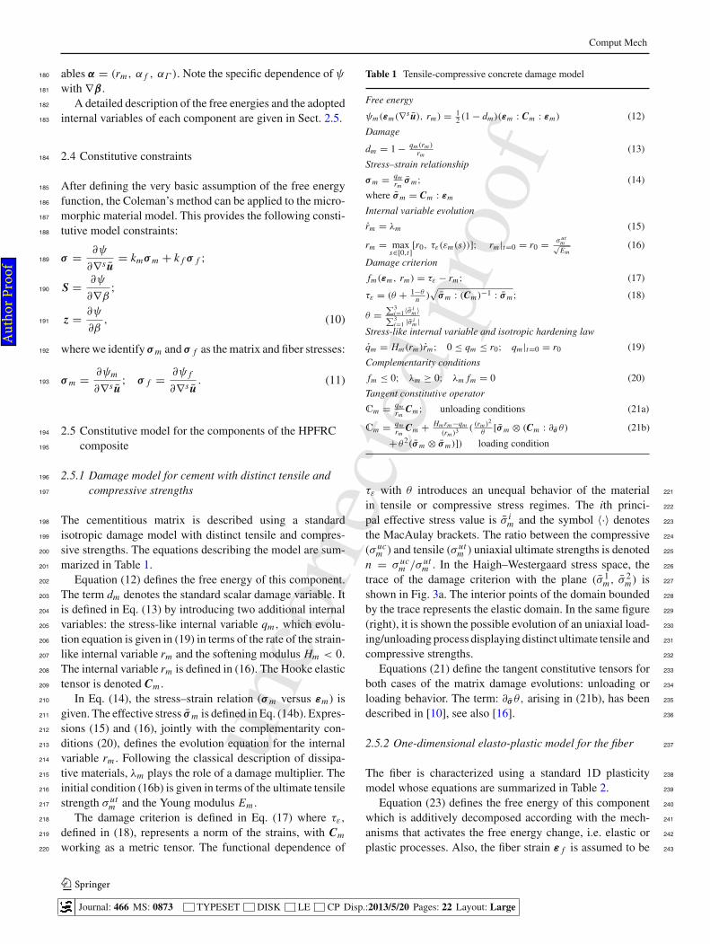
τε with θ introduces an unequal behavior of the material 221

in tensile or compressive stress regimes. The ith princi- 222

pal effective stress value is σ im and the symbol 〈·〉 denotes 223

the MacAulay brackets. The ratio between the compressive 224

(σ ucm ) and tensile (σ ut

m ) uniaxial ultimate strengths is denoted 225

n = σ ucm /σ ut

m . In the Haigh–Westergaard stress space, the 226

trace of the damage criterion with the plane (σ 1m, σ 2

m) is 227

shown in Fig. 3a. The interior points of the domain bounded 228

by the trace represents the elastic domain. In the same figure 229

(right), it is shown the possible evolution of an uniaxial load- 230

ing/unloading process displaying distinct ultimate tensile and 231

compressive strengths. 232

Equations (21) define the tangent constitutive tensors for 233

both cases of the matrix damage evolutions: unloading or 234

loading behavior. The term: ∂σ θ, arising in (21b), has been 235

described in [10], see also [16]. 236

2.5.2 One-dimensional elasto-plastic model for the fiber 237

The fiber is characterized using a standard 1D plasticity 238

model whose equations are summarized in Table 2. 239

Equation (23) defines the free energy of this component 240

which is additively decomposed according with the mech- 241

anisms that activates the free energy change, i.e. elastic or 242

plastic processes. Also, the fiber strain ε f is assumed to be 243

123


Au

tho

r P

ro

of

unco

rrec

ted

pro

of

Comput Mech

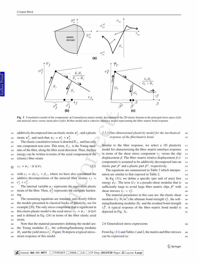
(a)

(b) (c)

Fig. 3 Constitutive model of the components. a Cementitious matrix model, description of the 2D elastic domain in the principal stress space (left)

and uniaxial stress versus strain plot (right), b fiber model and c cohesive interface model representing the fiber–matrix bond response

additively decomposed into an elastic strain: εef , and a plastic244

strain: εpf , and such that: ε f = εe

f + εpf .245

The elastic constitutive tensor is denotedE f , and has only246

one component non-zero. This term, E f , is the Young mod-247

ulus of the fiber, along the fiber axial direction. Then, the free248

energy can be written in terms of the axial component of the249

(elastic) fiber strain:250

ǫ f = ε f : (r ⊗ r), (22)251252

with ǫ f = (ur ),r + β,r , where we have also considered the253

additive decompositions of the uniaxial fiber strains: ǫ f =254

ǫef + ǫ

p

f .255

The internal variable α f represents the equivalent plastic256

strain of the fiber. Then, ψhf represents the energetic harden-257

ing.258

The remaining equations are standard, and closely follow259

the models presented in classical books of plasticity, see for260

example [20]. The only stress component that is significant in261

this elasto-plastic model is the axial stress: σ f = σ f : (r⊗r)262

and is defined in Eq. (24) in terms of the fiber elastic axial263

strain.264

Note that the material parameters defining the model are:265

the Young modulus E f , the softening/hardening modulus266

H f and the yield stress σyf . Figure 3b depicts a typical stress–267

strain response of this model.268

2.5.3 One-dimensional plasticity model for the mechanical 269

response of the fiber/matrix bond 270

Similar to the fiber response, we select a 1D plasticity 271

model for characterizing the fiber–matrix interface response 272

in terms of the shear stress component τ f versus the slip 273

displacement β. The fiber–matrix relative displacement β (r 274

component) is assumed to be additively decomposed into an 275

elastic part βe and a plastic part β p, respectively. 276

The equations are summarized in Table 3 which interpre- 277

tation are similar to that exposed in Table 2. 278

In Eq. (31), we define a specific (per unit of area) free 279

energy ψΓ . The term GΓ is a pseudo-shear modulus that is 280

sufficiently large to avoid large fiber–matrix slips βe with 281

shear stresses τΓ < τ uΓ . 282

The material parameters in this case are: the elastic shear 283

modulus GΓ N/m3) the ultimate bond strength τ uΓ , the soft- 284

ening/hardening modulus HΓ and the residual bond strength 285

τ RΓ . A typical response of the fiber–matrix bond model is 286

depicted in Fig. 3c. 287

2.6 Generalized stress expressions 288

From Eq. (11) and Tables 1 and 2, the matrix and fiber stresses 289

can be expressed as: 290

123


Au

tho

r P

ro

of

unco

rrec

ted

pro

of

Comput Mech

Table 2 Fiber 1D elasto-plastic model

Free energy

ψ f (ε f (∇s u, ∇β), α f ) = 12(εe

f : E f : εef ) + ψh

f (α f ) (23)

= 12

E f [ǫef ]2 + ψh

f (α f )

E f = E f (r ⊗ r) ⊗ (r ⊗ r); ε f = εef + ε

pf

Elastic stress–strain relationship

σ f = E f ǫef with ǫ f = (ur ),r + β,r (24)

Flow rule

ǫpf = λ f sign(σ f ) (25)


α f = λ f (26)

Isotropic hardening law

q f = H f (α f )α f (27)

Yield function

f f = |σ f | − (q f + σyf ) (28)


f f ≤ 0; λ f ≥ 0; λ f f f = 0 (29)


C f = C f [(r ⊗ r) ⊗ (r ⊗ r)] (30)

where C f ={

E f unloading conditionsE f H f

E f +H f; loading conditions

Table 3 Fiber–matrix interface 1D plastic model

Specific free energy

ψΓ (βe, αΓ ) = 12(βe · GΓ · βe) + ψh

Γ (αΓ ) (31)

= 12

GΓ [βe]2 + ψhΓ (αΓ );

GΓ = GΓ (r ⊗ r); β = βe + β p

Elastic stress–strain relationship

τΓ = GΓ βe (32)

Flow rule

β p = λΓ sign(τ f ) (33)


αΓ = λΓ (34)

Yield function

fΓ (τΓ , αΓ ) = |τΓ | − (qΓ + τ uΓ ) (35)

Isotropic hardening law

qΓ = HΓ (αΓ )αΓ (36)


fΓ ≤ 0; λΓ ≥ 0; λΓ fΓ = 0 (37)


CΓ = GΓ ; unloading condition

CΓ = GΓ HΓ

GΓ +HΓ; loading condition (38)

σm = ∂ψm

∂∇s u= (1 − dm) Cm : εm; (39)291

292

σ f = ∂ψ f

∂∇s u= σ f (r ⊗ r). (40)293

294

The microstress S are given by: 295

S = ∂ψ

∂∇β= µ f k f σ f (r ⊗ r), (41) 296

297

and the microforce z is: 298

z = ∂ψ

∂β= −δΓ

(

k f τΓ

)

r. (42) 299

300

Summarizing, the stresses of the different components can 301

be written as follows: 302

(i) matrix stress (given in Table 1): 303

σm = σm

(

εm

(

∇s u, rm

))

, 304

(ii) fiber stress (Table 2): 305

σ f = σ f

(

ǫ f

(

(ur ),r , β,r

)

, α f

)

, 306

(iii) interface stress (Table 3): 307

τΓ = τΓ

(

γ (β), αΓ

)

, 308

where the symbol (·) denotes the respective function. 309

2.7 The overall constitutive model of a HPFRC composite 310

having a random distribution of fiber bundles 311

The mechanical model of a HPRFC having a fiber bundle 312

in one direction, presented in the previous subsections, can 313

be generalized to account for a random distribution of fibers. 314

Let us consider a number n f of discrete fiber bundles in the 315

plane of analysis with a regular distribution of angles in the 316

interval: [0, π ]. 317

The Ith bundle, characterized with the supra-index I, 318

(I = 1, . . . , n f ), has assigned one volume fraction k If , one 319

direction vector rI and one micromorphic field β I = β(I )r(I )320

(supra-index in parenthesis indicates no-summation on this 321

index). 322

Adopting the mixture theory of Truesdell to account for 323

the macro/mesoscopic interactions, the free energy of the 324

HPFRC composite can be written as the linear combination 325

of the free energies of all its components, weighted by the 326

corresponding volume fraction: 327

ψ = kmψm +n f∑

I=1

k If ψ

If +

n f∑

I=1

k If ψ

IΓ . (43) 328

329

123


Au

tho

r P

ro

of

unco

rrec

ted

pro

of

Comput Mech

Then, the stress equation (10) results:330

σ = kmσm (εm; αm) +n f∑

I=1

k If σ

If

(

ε If

(

u, β I)

; α If

)

,

(44)

331

332

where σ If corresponds to the Ith fiber stress, given by Eq.333

(11)-b, along the direction rI .334

The tangent constitutive tensor of the composite: C =335

∂σ/∂ε, is given by:336

C = kmCm +n f∑

I=1

k If E I

f

[(

rI ⊗ rI)

⊗(

rI ⊗ rI)]

, (45)337

338

where E If is the Young modulus of the Ith fiber bundle.339

It is defined one fiber–matrix bond shear stress τ IΓ for340

every fiber bundle I th governed by a constitutive relation341

similar to that presented in Table 3.342

With this information in hand, one should be able to state343

the variational formulation as stated in next section.344

3 Variational formulation of the BVP345

Let us consider a body made of a HPFRC composite mate-346

rial which is modeled such as described in the preceding347

section. The governing equations of the BVP are: (i) the348

displacement–strain equations (3), (5)–(7), (ii) the consti-349

tutive equations, summarized in Tables 1, 2 and 3, and (iii)350

the balance equations (8a) and (8b) jointly with the bound-351

ary conditions. In the complete boundary of the body ∂B, we352

adopt: β I = 0 (I = 1, . . . , n f ).353

In order to introduce a variational approach of this prob-354

lem, we define the spaces of the kinematically admissible dis-355

placements: δu and morphological descriptor: δβ I for every356

fiber bundle I, as follows:357

V0 = {δu|δu = 0, ∀ x ∈ ∂Bu} ; (46)358

Vβ0 =

{

δβ I |δβ I = 0, ∀ x ∈ ∂B;(

I = 1, . . . , n f

)

}

.359

360

The variational equations of the BVP are presented in361

Table 4. Equation (47) is the variational expression of the362

balance equation (8a). And the variational equations (48),363

one for every index I, are obtained from the balance equa-364

tion (8b) after the following considerations:365

(i) we evaluate the average stress σ f (of the term σ f ) in the366

cross section of the fiber, and the average shear stress τΓ367

(of the term τΓ ) along the fiber circumferential perimeter.368

Then, we introduce both average stresses into the balance369

Table 4 Variational BVP

∫

Bσ : ∇sδu dB−

∫

Bb · δu dB −

∫

∂Bσt∗ · δu d S = 0; (47)

∀δu ∈ V0∫

B(Π I

AI τ If δβ

I + σ If (δβ

I ),r ) dB = 0; (48)

∀δβ(I ) ∈ Vβ0 ; (I = 1, . . . , n f )

equation (8b). In Eq. (48), Π I and AI are the perimeter 370

and area of one representative fiber of the fiber bundle I, 371

respectively. Both terms arise as a result of the averaging 372

process of the stresses in the fibers. 373

(ii) we consider identical models to those presented in Tables 374

2 and 3, to express the constitutive response of the aver- 375

aged stresses σ f and τΓ in terms of the averaged strain 376

quantities: ǫ f and γ ; and the model in Table 1. 377

Note that both expressions (47) and (48), in Table 4, have 378

been derived by weakening the derivative of the stress terms 379

and imposing the boundary conditions in the boundary inte- 380

grals. 381

Additional details of the variational BVP equations can 382

be seen in Oliver et al. [18]. 383

4 Finite element model 384

The finite element discretization of the displacement field 385

u ∈ H1(B) and micromorphic field β I ∈ H1(B) are now 386

considered. Both of them are interpolated using a standard 387

finite element technique: 388

u(x, t) =nnode∑

j=1

N j (x)q j (t); (49) 389

390

β I (x, t) =nnode∑

j=1

N j (x)p Ij (t); (50) 391

392

where N j are the shape functions of the finite element and q j 393

and p Ij are the displacement vector and the I th micromorphic 394

descriptor of the node j, respectively. The total number of 395

nodes in the finite element mesh is denoted nnode. While, the 396

corresponding variations are given: 397

δu(x, t) =nnode∑

j=1

N j (x)δq j (t); (51) 398

399

δβ I (x, t) =nnode∑

j=1

N j (x)δp Ij (t). (52) 400

401

123


Au

tho

r P

ro

of

unco

rrec

ted

pro

of

Comput Mech

Using Eq. (5), the interpolated strain terms in the finite402

element e can be written as follows:403

[εm]e =[

∇s u]e = Beqe, (53)404

405

where we have used the symbol [·] to represent the vec-406

tor Voigt notation of the corresponding tensor. The standard407

strain–displacement matrix Be of the element e is:408

Be =[

Be1 , Be

2,. . . ,Bene

node

]

;

Bej =

⎡

⎢

⎢

⎢

⎢

⎣

(

N ej

)

,x0

0(

N ej

)

,y(

N ej

)

,y

(

N ej

)

,x

⎤

⎥

⎥

⎥

⎥

⎦

,(54)409

410

with nenode being the number of nodes in element e, and the411

nodal displacement vectors of the same element e is denoted412

qe.413

From Eq. (6), the fiber strain vector, of the fiber bundle I,414

is:415

[

ε If

]e

= Beqe +(

T I1

[

N,r

]e + T I2

[

N,s

]e)

pI e, (55)416

417

where pI eis the nodal slip displacement vector of the same418

fiber bundle:419

pI e =[

p I1

e, p I

1

e, . . . , p I

nenode

e]T

, (56)420

421

and [N,r ], [N,s] are the r and s derivatives of the shape func-422

tion matrices:423

[

N,r

]

=[

(N1),r , . . . ,

(

Nnenode

)

,r

]

;

[

N,s

]

=[

(N1),s , . . . ,

(

Nnenode

)

,s

]

,

(57)424

425

where considering N j (x), then: (N j ),r = (N j ),x x,r +426

(N j ),y y,r . Also, matrices T I1 and T I

2 in Eq. (55), are the427

Voigt vector notation of the tensors: (rI ⊗ rI ) and (rI ⊗s sI ),428

respectively:429

T I1 =

[

r2x , r2

y , 2rxry

]T

I, (58a)430

431

T I2 =

[

rx sx , rxry,(

rx sy + rysx

) ]T

I. (58b)432

433

The axial component of the fiber strain I th can be written434

as follows:435

[

ǫ If

]e

=(

TI

1

)T [

ε If

]e

=(

TI

1

)T

Beqe +[

N,r

]e[

pI]e

,

(59)

436

437

where the projection operator: TI

1 is: 438

TI

1 =[

r2x , r2

y , rxry

]

, (60) 439

440

which satisfies: (TI

1)T T I

1 = 1 and (TI

1)T T I

2 = 0. 441

Finally, from Eq. (7), the strain vector representing the Ith 442

fiber–matrix slip mechanisms, is written: 443

[

γ I]

= T I2[N]epI e

. (61) 444

445

After introducing the finite element discretization into the 446

balance equations (47), (48) jointly with the constitutive rela- 447

tions in Tables 1, 2 and 3; the balance equations can be rewrit- 448

ten as a system of equations in the variables q, pI : 449

Ru

(

q, pI)

=nelem

Λe=1

∫

Be

(

Be)T

(

kmσm +n f∑

I=1

k If σ

If

)

dBe

− Fext = 0;

(62) 450

451

Rβ I

(

q, pI)

=nelem

Λe=1

k If

∫

Be

(

Π I

AI[N]eτ I

Γ + [N]e,r σ

If

)

dBe

= 0;(

∀I = 1, . . . , n f

)

,

(63)

452

453

where Fext is the vector of external forces, the symbol Λ 454

denotes the standard finite element assemblage operator, 455

nelem is the number of finite elements and Be identifies the 456

finite element domain of the element e. 457

4.1 Time integration scheme 458

The time integration problem consists of finding, at the time 459

step n + 1, the nodal displacements, qn+1, and micromor- 460

phic descriptors, p In+1, verifying the equations of the dis- 461

crete variational BVP (62), (63). We denote pn+1 the vector 462

collecting the slips pIn+1 of all fiber bundles. In those expres- 463

sions, the stresses: σm, σ If and τ I

Γ are explicit functions of 464

(qn+1, pn+1). Fext is evaluated at time (n + 1). 465

4.1.1 Solution of the coupled system of equations 466

Two general strategies can be adopted for solving the coupled 467

problem (62), (63): monolithic and fractional step methods 468

(also known as staggered techniques). The following items 469

describe both strategies. 470

(i) Monolithic scheme Solution of the nonlinear equations 471

(62), (63) are found using a Newton–Raphson algorithm, 472

123


Au

tho

r P

ro

of

unco

rrec

ted

pro

of

Comput Mech

which consists of, iteratively and simultaneously, determin-473

ing the increment of variables: (∆q; ∆p) by solving the lin-474

earized equation system derived from (62), (63):475

K

[

∆q

∆pI

]

= −[

Ru

Rβ I

]

, (64)476

477

where K is the Jacobian of the residuals (62), (63):478

K =∂([Ru; Rβ I ])∂([q; pI ]) =

nelem

Λe=1

[

K euu K e

uβ I

K eβ I u

K eβ I β I

]

. (65)479

480

The expression for K is obtained by introducing the strains481

(53), (59), (61) into the constitutive Tables 1, 2 and 3, deriving482

the corresponding stresses and then, introducing them into483

the derivatives of the residual terms defined in (62), (63).484

Following this procedure, every submatrix in (65) can be485

written as follows:486

Keuu =

∫

Be

(

Be)T

(

kmCm

+n f∑

I=1

k If C I

f

(

T I1 ⊗ T I

1

)

)

BedBe,

(66)487

488

Keuβ I =k I

f

∫

Be

(

(

Be)T

(

T I1C I

f

[

N,r

]e))

dBe, (67)489

490

Keβ I u

=k If

∫

Be

(

[

N,r

]eTC I

f T I1Be

)

dBe, (68)491

492

Keβ I β I =k I

f

∫

Be

(

Π I

AI[N]eT

C IΓ [N]e+

[

N,r

]eTC I

f

[

N,r

]e

)

dBe,

(69)

493

494

whereCm is the matrix constitutive tangent tensors defined in495

Eq. (21). And, C If and C I

Γ are the constitutive tangent tensor496

of every fiber bundle defined in (30) and (38), respectively.497

In order to preserve the notation as simple as possible, we498

do not specify the fact that, at step n + 1, expressions K and499

R in (64) are evaluated in every iteration k of the Newton–500

Raphson procedure.501

(ii) Staggered scheme In the second procedure, and taking502

advantage of the physical nature of the problem, the equa-503

tion system (62), (63) is partitioned into smaller and simpler504

subsystems. The solution of each subsystem determines one505

set of variables at a time, keeping fixed the remaining ones.506

For this specific problem, a natural partition consists of507

taking as many set of equations as families of fiber bundles508

exists: Rβ I = 0, for: I = 1, . . . , n f plus the equation of:509

Ru = 0.510

Then, given a prediction of the slip field (pI )Pn+1, which 511

are the linear extrapolations of values obtained in previous 512

time steps: 513

(

pIn+1

)P

= pIn +

(

pIn − pI

n−1

) ∆tn+1

∆tn, (70) 514

515

where ∆tn and ∆tn+1 are the time increments in steps n and 516

n + 1, respectively; the equation system: 517

Ru

(

qn+1,

(

pIn+1

)P)

= 0, (71) 518

519

is solved to find: qn+1. And this value is substituted, and 520

fixed, in each set of Eq. (63): 521

RβI

(

qn+1, pIn+1

)

= 0, (72) 522

523

which solution provides the slip values pIn+1. 524

After replacing (pIn+1)

P by pIn+1 in Eq. (71), the sequence 525

of operations to solve (71) and (72) are repeated iteratively 526

until obtaining the convergence of the equation system (62), 527

(63) at time step: n + 1. 528

The complete procedure is summarized in Table 5. 529

This scheme has two advantages with respect to the mono- 530

lithic one: (i) the staggered scheme provides a reduction in 531

the size of the matrices involved in the solution of each sub- 532

system, then, a significant saving in computational cost can 533

be expected, being more important when the number of fiber 534

bundles increase; and (ii) the computational treatment (han- 535

dling of dofs) of problems with a variable number of fiber 536

bundles is simpler. 537

Prediction (70) has shown to be successful to increase the 538

accuracy of the scheme. This effect can be seen in Fig. 4 that 539

represents the structural response of the beam in Sect. 5.2 540

when the effect of the interface zone vanishes (τ uΓ = 0). The 541

plots depicted in the figure are the load versus vertical dis- 542

placement of the load application point. Two solutions were 543

obtained with a staggered integration scheme using either: 544

(i) the extrapolation defined in (70), or (ii) without includ- 545

ing the extrapolation. Both curves have been evaluated using 546

the algorithm in Table 5 by removing the iterative proce- 547

dure (loop on the index k in the table). Thus, Eqs. (74) and 548

(75) have been evaluated only once per time step. In the last 549

case, when the predictor equation (73) is removed from the 550

algorithm, (pIn+1)

P is assumed to be (pIn+1)

P = pIn . Both 551

curves are compared with the monolithic procedure, which 552

solution has been evaluated using a full Newton–Raphson 553

procedure until convergence has been reached. All of those 554

solutions have been obtained with an identical time step 555

interval. 556

From the plots in Fig. 4, we conclude that the prediction 557

step defined in (70) introduces a significant improvement 558

123


Au

tho

r P

ro

of

unco

rrec

ted

pro

of

Comput Mech

Table 5 Staggered time

integration scheme using a

predictor step

LOOP over time steps: (n + 1)

(i) Prediction:(

pIn+1

)P = pIn + ∆pI ∆tn+1

∆tn∀I = 1, . . . , n f ; (73)

Initialize:(

pIn+1

)(0) =(

pIn+1

)P

(

pIn+1

)(−1) =(

pIn

)

;(

qn+1

)(0) = qn;WHILE NOT CONVERGED: iteration k

(ii) Solve nodal displacements: Given(

q(k−1)n+1 , pI (k−1)

n+1

)

Compute: Kuu; KuβI ; Ru and:

q(k)n+1 = q

(k−1)n+1 + (Kuu)−1

(

− Ru −∑n f

I=1 Kuβ I

(

pI (k−1)

n+1 − pI (k−2)

n+1

)

)

(74)

(iii) Solve nodal slip displacements: Given(

q(k)n+1, pI (k−1)

n+1

)

DO: I = 1, . . . , n f (loop on fibers)

Compute: KβIβI ; KβI u ; RβI and:

pI (k)

n+1 = pI (k−1)

n+1 +(

Kβ I β I

)−1(

− Rβ I − Kβ I u

(

q(k)n+1 − q

(k−1)n+1

)

)

(75)

END DO (loop on fibers)

END WHILE

END LOOP over time steps

0 0.2 0.4 0.6 0.8 1 1.2 1.4-5

0

5

10

15

20

25

(mm)

)N

k(F

Monolithic

Staggered(with predictor)

Staggered(without predictor)

Fig. 4 Structural response of the beam bending test (Sect. 5.2), com-

parison of different integration schemes. Two solution with a staggered

scheme (both of them: without global iteration) are depicted: (i) using

the predictor step of Eq. (70), and (ii) without using the predictor step.

For comparison, the solution of the monolithic procedure with full con-

vergence is also depicted

of the accuracy whenever only one evaluation of Eqs. (74)559

and (75) is performed (i.e., removing the loop k in Table560

5). In this case, we also note that the staggered scheme with561

extrapolation, during the strain softening regime, provides an562

slightly oscillatory response. The amplitude of these oscilla-563

tions decreases with the reduction of the time step length in 564

the time integration procedure. 565

4.1.2 Impl-Ex scheme 566

By adopting either of the two approaches presented in the pre- 567

vious subsection, it becomes necessary to solve non-linear 568

equation systems of the type Ru(σ (q, pI , α)) = 0 and 569

Rβ I (σ (q, pI , α)) = 0 simultaneously (monolithic scheme) 570

or sequentially (staggered scheme) as the time evolves. In 571

both cases, we remark the explicit dependence of these equa- 572

tions with the vector of internal variables: α. 573

The so-defined problem can be discretized in time by 574

assuming a standard implicit technique. Then, the variables 575

at step (n + 1), qn+1, pIn+1αn+1 and σ n+1, must be solved, 576

typically by means of a Newton–Raphson scheme. 577

However, it is well known that, when dealing with mate- 578

rial failure problems, the nonlinear equation systems result- 579

ing from a fully implicit discretization methodology show a 580

marked lack of robustness. 581

In Oliver et al. [15] and [14] an alternative algorithm, the 582

so called Impl-Ex algorithm, has been presented to reduce 583

the nonlinearity of the resulting equations without losing the 584

stability of the computed solution, which is very convenient 585

because it demands a very reduced computational cost. Here, 586

we describe a summary of this methodology that can be easily 587

adapted for modeling HPFRC composite. 588

123


Au

tho

r P

ro

of

unco

rrec

ted

pro

of

Comput Mech

At the time step (n+1), the internal variables of the model589

are evaluated through two integration procedures:590

(i) an implicit standard procedure, which determines, from591

Tables 1, 2 and 3, αn+1 and σ n+1;592

(ii) a predictor (explicit) procedure, here called Impl-Ex593

variable and denoted with the symbol (·), such as fol-594

lows:595

αn+1 = αn + ∆αn+1;

∆αn+1 = (αn − αn−1)∆tn+1

∆tn.

(76)596

597

After replacing these Impl-Ex internal variables into the598

constitutive equations, Tables 1, 2 and 3, the incremen-599

tal (rate) stress term, ∆σ n+1, is determined from these600

equations, and the Impl-Ex stress at time n + 1 is given601

by:602

σ n+1 = σ n + ∆σ n+1. (77)603604

The Eqs. (62) and (63) are then solved with the Impl-Ex605

stresses σ n+1 :606

Ru (σ n+1) = 0;Rβ I (σ n+1) = 0.

(78)607

608

It can be shown, see Oliver et al. [14], that, even during the609

material softening regime, the consistent tangent matrices,610

arising from this integration algorithm, are constant (during611

a time step) and positive definite. As a result of this property,612

only one iteration per time step is required to get convergence613

when the solution of Eq. (78) are searched through a Newton–614

Raphson procedure.615

Summarizing, the combination of: (i) a staggered scheme616

with the prediction stage of the previous subsection and617

removing global iterations for convergence, plus, (ii) the618

Impl-Ex procedure for solving each partition of the equation619

systems; defines a very robust algorithm for solving problems620

involving HPFRC composites with arbitrary distribution of621

fibers, which results in a very efficient methodology.622

4.2 Concrete fracture model623

The loss of the linear mechanical response in HPFRC com-624

posites depends on the crack phenomena happening in625

the cementitious component and its interaction with fibers626

through the fiber–matrix bond. Establishing a satisfactory627

constitutive model of a HPFRC composite material display-628

ing failure, then requires a concrete crack model that is629

strongly coupled with the fiber–matrix bond-slip mechanism.630

It is known that local constitutive models with strain soft-631

ening, such as the damage model presented in Table 1, leads to632

theoretical and numerical difficulties which reflect into spuri- 633

ous numerical solutions. The goal of a well-posed numerical 634

simulation tool is then to adopt a methodology providing 635

objective results respect to the finite element mesh, avoiding 636

the typical mesh size and bias dependence. 637

In the present approach, the mesh size dependence is 638

removed through the regularization of the softening model 639

of concrete. We reach this objective by introducing a model 640

characteristic length related to the finite element mesh size 641

and the fracture energy of the component. Thus, the soft- 642

ening modulus Hm in Table 1 is redefined, and replaced 643

in the table by the intrinsic softening modulus defined by: 644

Hm = −(G f Em/(σ utm )2)he, where G f is the concrete frac- 645

ture energy, Em and σ utm have been defined in Table 1 and 646

he is a representative finite element size consistent with the 647

crack orientation (see additional details in [13]). 648

As for removing the spurious mesh orientation depen- 649

dence, constants strain localization modes are injected, via a 650

mixed finite element formulation, such as proposed by Dias 651

et al. [5] and Dias [4], and summarized in the following sub- 652

section. 653

4.2.1 Strain injection method for computational modeling 654

of material failure 655

Let us consider standard irreducible quadrilateral finite ele- 656

ments, which are defined as the underlying elements. It is 657

well-known the flaws that this classical element shows for 658

capturing and simulating evolution of cracks. 659

In order to remove these flaws, we adopt a technique that 660

is mathematically consistent, based on a mixed (assumed 661

strain) variational formulation. This procedure is adopted 662

because it has been shown that mixed formulations, in gen- 663

eral, have much better abilities to capture and propagate 664

localizations modes if compared to irreducible formulations. 665

Assumed strain mixed formulation: the injection domain Let 666

us consider the material bifurcation analysis that is based on 667

detecting the singularity of the acoustic tensor: 668

det ([n · C (tB) · n]) = 0, (79) 669670

where C(tB) is the constitutive tangent tensor of the overall 671

response given by Eq. (45). Equation (79) provides the bifur- 672

cation time tB, as well as, the normal vector n to the possible 673

crack surface. The numerical resolution of the discontinuous 674

material bifurcation problem has been solved in an effective 675

and accurate way, using a numerical algorithm, based on the 676

iterative resolution of a coupled eigenvalue problem in terms 677

of the localization tensor. This algorithm has been presented 678

in Oliver et al. [17]. 679

After the criterion (79) has been satisfied in a given finite 680

element, we equip the element with an assumed strain model 681

123


Au

tho

r P

ro

of

unco

rrec

ted

pro

of

Comput Mech

that is formulated in the context of a mixed two-field (u−εm)682

variational approach. The interpolated displacement field683

remains the same as that of the irreducible quadrilateral finite684

element model presented at the beginning of this section, see685

Eq. (49). While, the strain field, εm, is interpolated with func-686

tions taken from Vε, where Vε is the space of element-wise687

constant functions. Then, strains εm are associated with dis-688

placements through the following variational equation:689

∫

B

(

εm − ∇s ˙u)

: δεdB = 0; ∀δε ∈ Vε. (80)690

691

From where, the strain matrix (53) in the element e can be692

written as:693

[εm]e = Beqe;

Be = 1

Be

∫

Be

BedBe = 0, (81)694

695

and Eq. (59) is consequently evaluated by using the modified696

strain–displacement matrix Be

instead of Be.697

The variational equilibrium expression (47), of Table 4, is698

rewritten as follows:699

∫

B

σ(

εe)

: δεdB −∫

B

b · δudB −∫

∂Bσ

t∗ · δu d S = 0;

∀δu ∈ V0; ∀δε ∈ Vε,

(82)700

701

and after replacing the interpolation of displacement and702

strain fields and changing the matrix Be by: Be, this equation703

can be identically written to the expression (62), (63).704

The domain where the constant strain mode is injected, is705

defined as the geometrical locus of the points satisfying:706

Bin j (t) := {X ∈ B|t ≥ tB(X); rm(X, t) > 0} , (83)707708

where the last condition (rm(X, t) > 0) means that the con-709

crete component of the composite should be evolving in a710

loading condition. It is a well known fact that the Assumed711

Strain Mixed formulation, given by (80) and (81), is unsta-712

ble if it is applied to the entire discrete domain. Then, it is713

important to inject the mixed formulation only in the reduced714

domain of the finite elements satisfying (83) (Fig. 5).715

For the numerical implementation of the injection proce-716

dure, it is selected the four node quadrilateral element with717

the standard four Gauss points with one additional Gauss718

points, placed in the central point of the element.719

Fig. 5 Strain injection domain

5 Assessments of the numerical model 720

In order to ascertain the suitability of the proposed formula- 721

tion for describing the structural response of the composite, 722

a selected set of experimental results is taken from the litera- 723

ture. Elastic, hardening and localization stages are examined. 724

The HPFRC composite model should reproduce two rele- 725

vant and influential mechanisms, namely, the fiber pullout 726

phenomenon and the subsequent fiber plasticity. In order 727

to show these model features, some tests are particularly 728

addressed in the following sections. 729

Physical observations of the HPFRC composite behavior 730

show that their failure modes primarily depends on the dis- 731

tribution, content and type of fibers within the specimen. In 732

the next numerical simulations, we show that the model pre- 733

dicts reasonably well the expected failure modes of HPFRC 734

composite with different contents of fibers. 735

The main concern in this section is to examine: (1) the 736

validation of the model, as well as, its predictive ability, (2) 737

evaluation of the injection procedure in order to improve the 738

finite element mesh-bias dependence during the strain local- 739

ization process, (3) the effect that the fiber–matrix interface 740

has on the failure mode description and the structural perfor- 741

mance. 742

In the following three cases, we adopt fibers having diam- 743

eters equal to: 3 mm. Then, the ratio Π/A = 1.33 mm−1. 744

Also, in all cases we have taken a residual bond strength: 745

τ RΓ = 0 MPa. 746

5.1 Notched strip under uniaxial loading 747

A notched strip (in plane strain) undergoing uniaxial loading 748

is simulated. The strip and loading conditions are shown in 749

Fig. 6a. It is clamped at its left end and pulled at the right 750

end. The notches are situated in the middle of the specimen to 751

ensure damage localization in this area. The region of concern 752

is the area close to the notch, where the pullout process is 753

expected. 754

In this test, the complex interaction between the meso- 755

scopic phenomenon such as: the cement fracture, the fiber– 756

matrix debonding and the fiber plasticity, can be more easily 757

comprehended and evaluated. 758

123


Au

tho

r P

ro

of

unco

rrec

ted

pro

of

Comput Mech

(a)

(a)

Fig. 6 Notched strip under uniaxial loading: a test setup, b comparison

between load versus displacement curves using different ultimate bond

shear stresses

The fiber pullout mechanism is analyzed when the fibers759

are parallel to the principal stretch direction.760

5.1.1 Tensile behavior of the specimen with aligned steel761

fibers762

Numerical simulations with identical mechanical and geo-763

metrical characteristics are carried out, but varying the bond764

properties of the fiber–matrix interface. The set of parameters765

is summarized in Table 6. In order to investigate the sensi-766

tivity of the model with the ultimate matrix–fiber bond shear767

strength, τ uΓ , six different values of this parameter are con-768

sidered. While, only one horizontally oriented fiber bundle769

is assumed (θ = 0◦).770

Figure 6b compares the load P versus displacement δ771

response of the specimen for the six values τ uΓ . Included772

in the plots are the structural response of the plain concrete.773

The ascending behavior of the responses are characterized,774

as we will explain later, by bonded, or partially debonded,775

matrix–fiber interfaces. As it may be surmised, the hardening776

behavior is related to the debonding process.777

To understand these numerical results, we recall from778

experimental tests that the HPFRC composites, in tension,779

Table 6 Material parameters of the notched specimen under uniaxial

loading

Matrix Fiber Bond (fiber–matrix)

σ utm = 2.0 MPa σ

yf = 210 MPa τ u

Γ = 0.001, 0.1, . . .

. . . 0.6, 1, 5, 50 MPa

Em = 15.0 GPa E f = 200 GPa GΓ = 1.e8 GPa

νm = 0.2 H f = 0 MPa HΓ = 100 MPa

G f = 100 N/m θ = 0◦ k f = 0.75 %

displays three stages: linear elastic (that ends when the first 780

crack in the specimen arises), multicrack or hardening stage 781

(that ends at the peak point), and the strain localization 782

stage. Also we recall that, in the tensile load–displacement 783

response, the main difference between the HPFRC compos- 784

ite and the conventional FRC is the multicrack stage after 785

finalizing the linear response. The multicrack stage may not 786

exist in the conventional FRC. 787

The response for the smallest value of the ultimate bond 788

shear stress considered in this example, τ uΓ = 0.001 MPa, 789

closely resembles the curve displayed by the plain concrete 790

case. As expected, the numerical results show brittle behav- 791

ior for the plain concrete material. After the peak load has 792

been reached, the material softens and ductility is barely evi- 793

denced. 794

The load–displacement curves for increasing values of τ uΓ 795

display increasing hardening, as well as, increasing peak load 796

values. However, with τ uΓ > 5 MPa, the response of the 797

material no longer change significantly. Then, in the present 798

specific problem, we could assert that τ uΓ = 5 MPa represents 799

a limit bond strength. 800

Figure 7 depicts the iso-color maps of damage distribution 801

in cement at the end of analysis. Different cases, depending 802

on τ uΓ , are shown. Figure 7a displays the tendency of the plain 803

concrete response showing a highly concentrated damage 804

pattern. With increasing τ uΓ , according with Fig. 7b:f, the 805

zone affected by damage grows, suggesting that an increasing 806

number of fibers are subjected to the pullout effect, and, in 807

consequence, the material toughness increases. 808

Analysis of the interaction effects between matrix, fiber and 809

interface debonding For identical time steps, sequential por- 810

traits of plasticity in fibers, matrix damage and matrix–fiber 811

interface debonding distributions can be superimposed to 812

visualize the failure characteristics of each compound. The 813

analysis, at the microstructural level, reveals various failure 814

mechanisms which synergistic interaction accounts for the 815

larger strength and higher toughness properties. The analysis 816

is performed with four values of τ uΓ = [0.001, 1, 5, 50 MPa. 817

In concordance with these values, we distinguish three differ- 818

ent failure mechanisms, depending on the fiber–matrix bond 819

responses: (i) fully debonded fibers, (ii) partially debonded 820

123


Au

tho

r P

ro

of

unco

rrec

ted

pro

of

Comput Mech

Fig. 7 Damage distribution in cement matrix with different matrix–

fiber bond strength parameters

fibers and (iiii) fully bonded fibers. They are specifically ana-821

lyzed in the following items.822

(i) Fully debonded fibers: (τ uΓ = 0.001 MPa)823

Weak fiber–matrix interfaces are generally associated to824

a low fracture toughness of the composite. A weak inter-825

face posses low fiber–matrix stress transfer capacity and,826

therefore, the fiber strengths are not fully utilized. Accord-827

ing to the results in Fig. 6b, low ductility is associated with828

τ uΓ = 0.001 MPa. Under tensile loads, the model shows a829

sudden debonding in the whole domain, as it is observed in830

the debonding distribution of Fig. 8 with a consequent loss of831

the material composite effect. In this case, we verify that for832

enough small values of the ultimate bond strengths, the model833

is able to represent weak fiber–matrix interfaces. In fact, this834

(a)

(c)

(d)

12

3

4

)N(

P

(mm)

(b)

0 10 20 30 40 50 60 70-0.05

0

0.05

0.1

0.15

x-coordinate (mm)

0 10 20 30 40 50 60 70

-0.1

-0.05

0

0.05Slip

x-coordinate (mm)

ux

12

3

4

123

4

x

Fig. 8 Results for τ uΓ = 0.001 MPa. a Distribution portraits of fiber

plasticity, fiber–matrix interface debonding and matrix damage at the

end of analysis. The fiber–matrix interface debonding map is repre-

sented with only two states: 0 is no-debonding (τΓ < τ uΓ ), 1 is debond-

ing meaning that in some loading stage (τΓ = τ uΓ ). Damage map ranges

between 0 and 1, b load versus displacement curve, c ux displacement

plot along the specimen horizontal direction (numbers are in correspon-

dence with the loading stages shown in b), d plots of the fiber–matrix

slip β along the specimen horizontal direction (numbers are in corre-

spondence with the loading stages shown in b)

is a consequence of the Capriz balance equation, which gov- 835

erns the microstructural behavior. When using τ uΓ ≈ 0 MPa, 836

the fiber strain also approaches to zero, and therefore, the 837

fiber is pulled out from the matrix immediately after the load 838

is applied. Also, this implies that the slip β can take any arbi- 839

trary value after the bond strength is exhausted. Certainly, 840

the value of the slip is of the same order of magnitude than 841

the displacement ux , as shown in Fig. 8c, d, where the slip β 842

and ux displacement are plotted along the length of the strip 843

123


Au

tho

r P

ro

of

unco

rrec

ted

pro

of

Comput Mech

(a)

(b)

1

2)N(

P

(mm)

Fig. 9 Results for τ uΓ = 1 MPa. Distribution portraits of fiber plastic-

ity, fiber–matrix interface debonding and matrix damage at the end of

analysis: a stage 1 at the softening regime onset. b Stage 2 in the end

of the loading process

in different stages of the loading curve as indicated in Fig.844

6b. Damage concentration in the notch section is due to the845

inability of the fiber–matrix interface to transfer the stresses.846

According with the damage and debonding results in Fig. 7,847

small axial strain in the fibers is developed due to the sud-848

den debonding, and consequently, yielding is not achieved,849

as confirmed in the fiber plasticity distribution.850

(ii) Partially debonded fibers: (τ uΓ = 1 MPa)851

In the case simulated with τ uΓ = 1 MPa, which in accor-852

dance with the Fig. 6 displays semi-ductile behavior, rep-853

resents a partially debonded example. The results obtained854

in this case are shown in two different instants indicated in855

Fig. 9. The first instant, Fig. 9a, represents a stage during the856

hardening process. The second instant, Fig. 9b, represents a857

stage at the end of the localization process.858

The assumed perfect plastic material behavior adopted for859

the matrix–fiber bond slip relationship gives rise to the slip860

when the ultimate bond shear strength is reached, and subse-861

quently the shear deformation is increased. In the first instant,862

depicted in Fig. 9a, it is noticeable that fiber–matrix interface863

(a)

(b)

Fig. 10 Distribution portraits of fiber plasticity, fiber–matrix interface

debonding and matrix damage at the end of analysis: a results for τ uΓ =

5 MPa. b Results for τ uΓ = 50 MPa. Scales of the iso-colour maps for

the plasticity, damage and debonding distributions are similar to the

description given in the legend of Fig. 9

debonding evolves as a consequence of the increase in the 864

slip. Fiber–matrix interface debonding and matrix damage 865

may be triggered because of their weakness to resist shear 866

stresses. This behavior indicates that the matrix damage and 867

sliding frictional resistance of fiber pullout largely determine 868

the composite toughness and the hardening properties (Bey- 869

erlein and Phoenix [2]). Inspection of the plots for damage 870

and plasticity in the second stage, Fig. 9b, indicates that the 871

crack opening in the notch, due to cumulative damage, is 872

accompanied with loss of adhesive bond in the matrix–fiber 873

interface and plastic strain in fibers. 874

After comparing the debonding maps of stage 2 in Fig. 9 875

with those of stage 1, we note that only few more points in 876

the specimen achieve the ultimate bond shear strength at the 877

end of analysis. 878

(iiii) Fully bonded fibers to the matrix: (τ uΓ = 5 − 879

−50 MPa) 880

High adhesive interfaces can be achieved by improv- 881

ing, at microstructural level, the properties of fiber surface. 882

123


Au

tho

r P

ro

of

unco

rrec

ted

pro

of

Comput Mech

(a)

(b)

(c)

1

3

46

7

5

2

F

Plain concrete

Experimental(Bencardino et al.)

Numerical

(mm)

)N

k (F

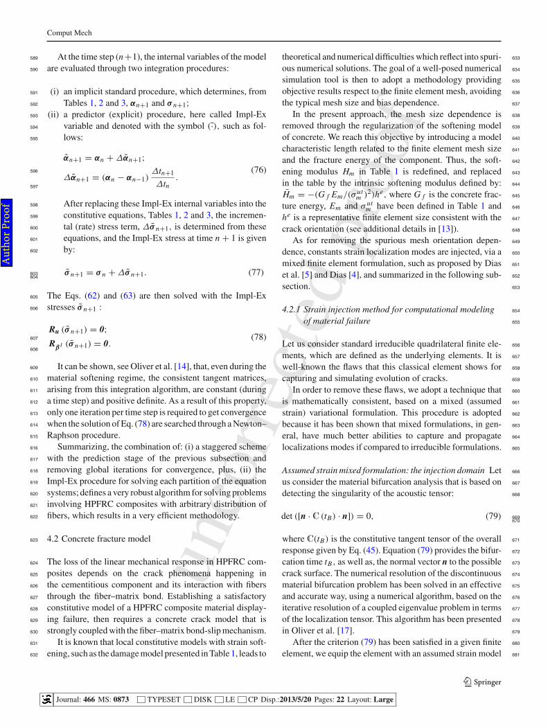
Fig. 11 Notched three point beam bending test with randomly distrib-

uted fibers. a Specimen geometry, b numerical and experimental load F

versus vertical displacement δ of the loading application point in three

point notched beam test

Table 7 Material parameters adopted in the model to simulate the

notched beam specimen test under flexural loading


σ ucm = 21.25 MPa σ

yf = 2100 MPa τ u

Γ = 5.1 MPa


νm = 0.2 H f = 100 MPa HΓ = 100 MPa

G f = 100 N/m θ = [0◦, 10◦, 20◦, k f = 1 %

30◦, 45◦, 60◦,

70◦, 80◦, 90◦]

However, a strong interface may result in lower toughness,883

because this effect does not allow interfacial debonding,884

which is one of the main mechanisms to relieve stress concen-885

trations produced by the oncoming crack (Jiang et al. [7]).886

With a view towards investigating this possibility, simula-887

tions were performed for τ uΓ = 5 and 50 MPa.888

(b)(a)

(c)

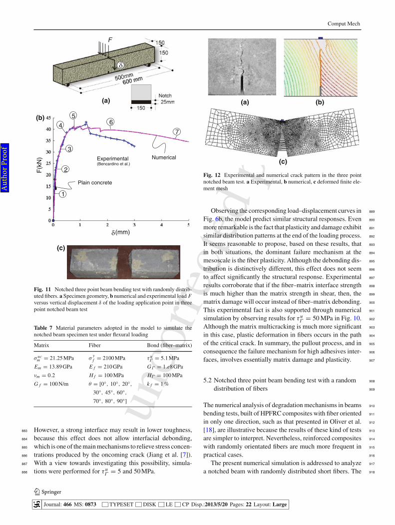
Fig. 12 Experimental and numerical crack pattern in the three point

notched beam test. a Experimental, b numerical, c deformed finite ele-

ment mesh

Observing the corresponding load–displacement curves in 889

Fig. 6b, the model predict similar structural responses. Even 890

more remarkable is the fact that plasticity and damage exhibit 891

similar distribution patterns at the end of the loading process. 892

It seems reasonable to propose, based on these results, that 893

in both situations, the dominant failure mechanism at the 894

mesoscale is the fiber plasticity. Although the debonding dis- 895

tribution is distinctively different, this effect does not seem 896

to affect significantly the structural response. Experimental 897

results corroborate that if the fiber–matrix interface strength 898

is much higher than the matrix strength in shear, then, the 899

matrix damage will occur instead of fiber–matrix debonding. 900

This experimental fact is also supported through numerical 901

simulation by observing results for τ uΓ = 50 MPa in Fig. 10. 902

Although the matrix multicracking is much more significant 903

in this case, plastic deformation in fibers occurs in the path 904

of the critical crack. In summary, the pullout process, and in 905

consequence the failure mechanism for high adhesives inter- 906

faces, involves essentially matrix damage and plasticity. 907

5.2 Notched three point beam bending test with a random 908

distribution of fibers 909

The numerical analysis of degradation mechanisms in beams 910

bending tests, built of HPFRC composites with fiber oriented 911

in only one direction, such as that presented in Oliver et al. 912

[18], are illustrative because the results of these kind of tests 913

are simpler to interpret. Nevertheless, reinforced composites 914

with randomly orientated fibers are much more frequent in 915

practical cases. 916

The present numerical simulation is addressed to analyze 917

a notched beam with randomly distributed short fibers. The 918

123


Au

tho

r P

ro

of

unco

rrec

ted

pro

of

Comput Mech

(a) 0ο (b) 45 (c) 90

1

3

4

6

7

ο ο

Fig. 13 Evolution of the matrix–fiber debonding process in the notched beam test for three fiber bundles directed along 0◦, 45◦ and 90◦ respect

to the horizontal direction. Stages 1, 3, 4, 6 and 7 correspond to the points marked in Fig. 11b

(a) 0ο (b) 45ο

(c) 90ο

1

3

4

6

7

Fig. 14 Evolution of fiber plasticity in three point notched beam test for three fiber bundles directed along 0◦, 45◦ and 90◦ respect to the horizontal

direction. Stages 1, 3, 4, 6 and 7 correspond to the points marked in Fig. 11b

experimental test corresponding to this case has been pre-919

sented by Bencardino et al. [1], and has been carried out920

according to the RILEM specification [19]. The beam geom-921

etry is shown in Fig. 11a.922

In Table 7, we define the mechanical properties adopted in923

the numerical model for the matrix, fiber bundles and fiber–924

matrix interface. Also, we assumes that nine fiber bundles925

represent sufficiently well the random distribution of fibers.926

The finite element model, assumed as a plane stress condi-927

tion, consists of 3,938 quadrilaterals with 4,032 nodes.928

The experimental load versus displacement curve, of a929

FRC specimen with fiber fraction volume equal to 1 %, is930

presented in Fig. 11b, (taken from Bencardino et al. [1]). In 931

the same plot, we compare the numerical solution. Experi- 932

mental and numerical curves agree quite well up to the peak 933

load. However, after this point, the numerical model slightly 934

overestimates the postcritical response. Also, in the same 935

plot, the experimental unreinforced (plain concrete) speci- 936

men is shown. A brittle behavior is observed. 937

5.2.1 Mesostructural behaviour 938

In the experimental test, a complete separation of the speci- 939

mens into two parts has occurred, as shown in Fig. 11c. The 940

123


Au

tho

r P

ro

of

unco

rrec

ted

pro

of

Comput Mech

1

3

4

7

5

2

Fig. 15 Damage evolution in three point notched beam test

Fig. 16 Double-notched dogbone specimen tensile test (Suwannakarn

[21])

finite element simulation also predicts a single crack, see Fig.941

12a:b. However, the specimen does not split abruptly in two942

parts as for the unreinforced beam. The deformed configura-943

tion of the beam after loading is scaled by 10 in Fig. 12c.944

Figures 13 and 14 display the evolution of the simulta-945

neous capacity loss of matrix–fiber bound, as well as, the946

plastic strains of fibers, respectively. Three bundles of fibers947

(b)(a)

Fig. 17 Double-notched dogbone specimen tensile test: a test layout,

b finite element mesh

Table 8 Material parameters


σ utm = 1.25 MPa σ

yf = 2100 MPa τ u

Γ = 5.1 MPa


νm = 0.2 H f = 100 MPa HΓ = 100 MPa

G f = 100 N/m θ = [0◦, 10◦, k f = 0.75 %

20◦, 30◦, 45◦,

60◦, 70◦, 80◦,

90◦]

Fig. 18 Numerical and experimental structural response in double

notched dogbone test. Average stress versus δ displacement. (a) Numer-

ical. (b) Experimental (Suwannakarn [21])

(oriented to 0◦, 45◦ and 90◦) and different stages along the 948

load deflection curve are specifically analyzed. According 949

to these results, the evolution of both mechanisms are con- 950

123


Au

tho

r P

ro

of

unco

rrec

ted

pro

of

Comput Mech

(3)(2)(1)

(a)

(b)

(c)

Fig. 19 Tensile response in double notched test: a typical crack propagation and strain localization in HPFRC composites as described in Suwan-

nakarn [21], b damage distribution (d ≥ 0.98), c iso-displacement curves displaying the macrocrack formation and evolution

centrated in the region near the notch, where crack propa-951

gation is expected to occur. The attention is addressed ini-952

tially to analyze the debonding distribution of the fiber bun-953

dles oriented 0◦ and 45◦ respect to the horizontal direc-954

tion (Fig. 13a, b, respectively). These results suggest that955

the loss of the adhesion in the interface zone starts during956

the initial loading stages. However, for the bundle fiber ori-957

ented 90◦, Fig. 13c, the distribution displays that the process958

begins later and it does not affect the area located near the959

notch.960

5.2.2 Damage evolution and localization process961

Microcracking in the cement matrix occurs simultaneously962

with debonding and plasticity of fibers during the fracture963

process. Figure 15 displays the iso-color damage maps in six964

different stages that are identified in the load versus displace-965

ment plot of Fig. 11b.966

In the stages 1 and 2, few elements around the notch are967

damaged. As loading progresses, the damage region spreads968

over beyond the notch section. In the stage 3, some elements969

in the bottom part of the beam begin to damage. From stage970

3, the damaged region covers the middle third and remains 971

almost unaltered until the end of the loading process. Darker 972

red color stands for completed damage material. According 973

to the iso-color map in the stage 7, severe degraded material is 974

presented in the notch proximity. However, comparing this 975

result and the iso-displacement contours in Fig. 12b only 976

a single vertical macrocrack, initiated in the notch root, is 977

developed. 978

5.3 Double-notched dogbone specimen tensile test 979

According with Suwannakarn [21], from where we take the 980

experimental results of this test, the dogbone-shaped notched 981

specimen is well adapted to control the location of the crack 982

position. To ensure an adequate propagation path, the speci- 983

men has symmetrical notches at their mid section. Addition- 984

ally, this test setup is useful to measure the composite fracture 985

properties of HPFRC composites and estimate the size of a 986

pseudo-plastic zone which corresponds to the cracked area 987

of the matrix. 988

The geometric details of the specimen are shown in Fig. 989

16. Dimensions are given in Fig. 16b, c for the longitudinal 990

123


Au

tho

r P

ro

of

unco

rrec

ted

pro

of

Comput Mech

(3)(2)(1)

(a)

(b)

(c)

(d)

Fig. 20 Main stages of debonding and plasticity evolution of the loading process in the dogbone test. a Debonding distribution (fiber bundle:

θ = 0◦). b Plasticity distribution (θ = 0◦). c Debonding distribution (fiber bundle: θ = 90◦). d Plasticity distribution (θ = 90◦)

and cross section, respectively. The loading process consists991

of imposing displacements at the specimen top, while fixing992

the bottom, as indicated in Fig. 17a.993

The material parameters for this example are summarized994

in Table 8. The specimen is reinforced with hooked end fibers995

and has a fiber volume fraction of 0.75 %. The test is simu-996

lated using 1,639 quadrilateral finite elements in plane stress997

condition. In order to capture the concrete fracture phenom-998

ena, we adopt the formulation presented in the previous sec-999

tion based on the injection of constant strain localized modes.1000

The finite element mesh is shown in Fig. 17b.1001

Figure 18 plots the stresses versus crack opening displace-1002

ments obtained with the numerical simulation. This result is1003

compared with the envelope of the experimental tests which1004

were obtained with a small number of specimens (only 3).1005

In both, numerical and experimental results, can be observed1006

that after the initial elastic response, the structural behav-1007

ior displays a hardening effect even when a multiple crack1008

phenomena is developing. The numerical result follows this1009

trend and lies within the experimental envelopes. However,1010

after crossing the peak load value, the numerical solution 1011

deviates from the experimental data. 1012

5.3.1 Crack propagation analysis in the notched hooked 1013

end fiber specimen 1014

In Fig. 19, we analyze the crack propagation phenomenon. 1015

The numerical solution displays a fracture process starting 1016

in the roots of the specimen notches, such as observed by 1017

Suwannakarn. And cracks evolve in a similar manner to that 1018

described in Fig. 19a. 1019

There are three main stages represented in Fig. 19 corre- 1020

sponding to: the onset of the first crack (column 1 of pictures), 1021

multiple cracks, associated with strain hardening (column 2), 1022

and (3) the strain localization stage, associated with strain 1023

softening (column 3). 1024

As the specimen is subjected to tensile loads, damage con- 1025

centration arises mostly at the notch root proximity, as it is 1026

shown in the first stage of Fig. 19b. After initiation, the dam- 1027

age extends in several directions (stage 2 of Fig. 19b). A large 1028

123


Au

tho

r P

ro

of

unco

rrec

ted

pro

of

Comput Mech

Fig. 21 Failure mode in the

double notched test. a

Numerical. b Experimental

(Suwannakarn [21])

(a) (b)

damage zone is observed during this stage, but the macro-1029

cracks formed at the notch roots do not propagate, proba-1030

bly arrested by the fibers. According to Suwannakarn, the1031

first crack does not necessarily propagates across the sec-1032

tion, prior to the formation of other cracks. The numerical1033

results have captured this effect.1034

Figure 19c shows iso-displacement contours plot in the1035

three considered stages. As can be seen in the contour1036

plots, the macrocrack propagates from the notch roots to1037

the specimen center, nonetheless, branching at the notches1038

is observed in the initial stages, so that more than one crack1039

are competing.1040

Pictures in Fig. 20 compares the debonding and plastic1041

evolution in the fiber bundles oriented at angles: θ = 0◦1042

and 90◦ respect to the loading direction. Observing Fig. 20b,1043

c, they suggest that the pullout process involves initially, a1044

debonding action, which provides several alternative paths1045

for the crack propagation. And second, fiber plastic defor-1046

mation, which contributes directly to the total deformation1047

of the composite. According with these results, the debond-1048

ing action is preceded by the formation of new surfaces at1049

the fiber–matrix interface; therefore, reduction of composite1050

strength may be significantly related to the loss of interface1051

resistance. Figure 20d also reveals that plastic deformation1052

is not observed in horizontally placed fiber bundles. How-1053

ever, debonding plots in Fig. 20c predict loss of adhesive and1054

frictional capacity in the interface zone.1055

Iso-displacement contours for total displacements (|u‖),1056

in Fig. 21a, shows a single macrocrack between the two sym-1057

metrical notches. This crack pattern agrees with the exper-1058

imental observation of the three specimens depicted in Fig.1059

21b. The fractured specimens are depicted on the right hand1060

side of the Fig. 21. Since the presence of the notches in the1061

specimen was designed to induce stress concentration in the 1062

central region and, in turn, an easy predictability of the crack 1063

pattern, nevertheless, experimental findings partially reflect 1064

this assertion and show in one case (according to Suwan- 1065

nakarn) a deviated crack path respect to the desired trajectory 1066

(Fig. 21b, left). 1067

6 Conclusions 1068

Considering the numerical solutions of problems solved in 1069

Sect. 5, as well as, those complementing the set of valida- 1070

tion tests that were presented in the paper of Oliver et al. 1071

[18] using the identical micromorphic model; we conclude 1072

that, the numerical approach developed for simulating fail- 1073

ure of HPFRC composites is able to capture important effects 1074

induced by the concrete fracture and the mechanical interac- 1075

tion between fiber and matrix. 1076

Some parameters that are explicitly considered in the 1077

model, and which dramatically affect the composite response 1078

leading to the complete failure, are: quantity of fibers, yield 1079

strength of fibers and strength of cement. Other important 1080

parameters, such as the fiber shape, roughness of the fiber 1081

surface, fiber aspect ratio, etc., have been implicitly consid- 1082

ered through a phenomenological law describing the shear– 1083

slip interaction in the fiber–matrix interface. The numerical 1084

assessments have highlighted the influence of some of these 1085

parameters in the structural responses. 1086

The model introduces as many slip displacement fields, 1087

and microscopic balance equations, as fiber bundles are con- 1088

sidered in the composite. Therefore, a variable number of 1089

dof’s per node have to be managed. We have proposed a very 1090

efficient numerical procedure to handle this specific feature 1091

123


Au

tho

r P

ro

of

unco

rrec

ted

pro

of

Comput Mech

of the problem. It is based on a partitioning of the macro- and1092

microforce balance equations, a predictor step of the slip dis-1093

placement fields, one for every fiber bundle, and the Impl-Ex1094

integration scheme.1095

The concrete fracture model included in the numerical1096

procedure uses a technique that is not affected by the finite1097

element mesh [4].1098

The notched strip results obtained with the simulation1099

model in Sect. 5.1, exemplifies the use of this computational1100

tool. The conclusions obtained from this test, and particu-1101

larly those obtained in the analysis of the three main cases of1102

bonding in cementitious composites, can be extended to the1103

analysis of more complex situations.1104

In the tests presented in Sects. 5.2 and 5.3, we have ana-1105

lyzed the effect of fiber plasticity and debonding as a function1106

of the inclination angle of the fiber respect to the load direc-1107

tion. However, there is one mesoscopic effect that the model1108

do not address specifically. In fact, we have assumed that the1109

shear stress-slip law characterizing the mechanical response1110

of the bond, in the fiber–matrix interface, does not changes1111

with the direction of the fiber. According to Lee at al. [8],1112

due to the mechanisms of snubbing, matrix spalling and1113

fiber straightening, these law changes notably with the fiber1114

direction. Future research should be addressed to include this1115

important phenomenon in the numerical model.1116

Acknowledgements J. Oliver gratefully acknowledges the financial1117

support of the European research Council (ERC) through the 2012- ERC1118

Advanced Grant Project No. 320815. The Spanish Ministry of Science1119

and Innovation, and the Catalan Government Research Department, are1120

also gratefully acknowledged for their financial support to this research1121

under Grants BIA2011-24258 and 2009 SGR 1510, respectively.1122

References1123

1. Bencardino F, Rizzuti L, Spadea G, Swamy RN (2010) Experi-1124

mental evaluation of fiber reinforced concrete fracture properties.1125

Composites B 41:17–241126

2. Beyerlein IJ, Phoenix SL (1996) Stress concentrations around mul-1127

tiple fiber breaks in an elastic matrix with local yielding or debond-1128

ing using quadratic influence superposition. J Mech Phys Solids1129

44:1997–20391130

3. Capriz G (1989) Continua with microstructure. Springer, Berlin1131

4. Dias IM (2012) Strain injection techniques in numerical modeling1132

of propagating material failure. PhD Thesis, Technical University1133

of Catalunya, Barcelona1134

5. Dias IF, Oliver J, Huespe AE (2011) Strain injection, mixed for- 1135

mulations and strong discontinuities in fracture modeling of quasi- 1136

brittle materials. In: Proceedings of the congress on numerical 1137

methods in engineering 2011, Coimbra, Portugal, 14–17 June, 1138

2011, pp 163–202. APMTAC, LIsbon 1139

6. Frémond M, Nedjar B (1996) Damage, gradient of damage and 1140

principle of virtual power. Int J Solids Struct 33:1083–1103 1141

7. Jiang H, Valdez JA, Zhu YT, Beyerlein IJ, Lowe TC (2000) The 1142

strength and toughness of cement reinforced with bone-shaped steel 1143

wires. Compos Sci Technol 60:1753–1761 1144

8. Lee Y, Kang S, Kim JK (2010) Pullout behaviour of inclined steel 1145

fibers in an ultra-high strength cementitious matrix. Constr Build 1146

Mater 24:2030–2041 1147

9. Li F, Li Z (2000) Continuum damage mechanics based modeling of 1148

fiber reinforced concrete in tension. Int J Solids Struct 36:777–793 1149

10. Linero DL (2006) A model of material failure for reinforced con- 1150

crete via Continuum Strong Discontinuity Approach and mix- 1151

ing theory. PhD Thesis, E.T.S. Enginyers de Camins, Canals i 1152

Ports, Technical University of Catalonia (UPC), Barcelona, 2006. 1153

CIMNE Monograph Number, M106 1154

11. Mariano PM (2002) Multifield theories in mechanics of solids. Adv 1155

Appl Mech 38:1–93 1156

12. Mariano PM, Stazi F (2005) Computational aspects of the mechan- 1157

ics of complex materials. Arch Comput Methods Eng 12:391–478 1158

13. Oliver J (1989) A consistent characteristic length for smeared 1159

cracking models. Int J Numer Methods Eng 28:461–474 1160

14. Oliver J, Huespe AE, Blanco S, Linero DL (2005) Stability and 1161

robustness issues in numerical modeling of material failure with 1162

the strong discontinuity approach. Comput Methods Appl Mech 1163

Eng 195(52):7093–7114 1164

15. Oliver J, Huespe AE, Cante JC (2008a) An implicit/explicit inte- 1165

gration schemes to increase computability of non-linear material 1166

and contact/friction problems. Comput Methods Appl Mech Eng 1167

197:1865–1889 1168

16. Oliver J, Linero DL, Huespe AE, Manzoli O (2008b) Two- 1169

dimensional modeling of material failure in reinforced concrete 1170

by means of a continuum strong discontinuity approach. Comput 1171

Methods Appl Mech Eng 197:332–348 1172

17. Oliver J, Huespe AE, Cante JC, Diaz G (2010) On the numerical 1173

resolution of the discontinuous material bifurcation problem. Int J 1174

Numer Methods Eng 83:786–804 1175

18. Oliver J, Mora D, Huespe AE (2012) A micromorphic model for 1176

steel fiber reinforced concrete. Int J Solids Struct 49:2990–3007 1177

19. R. T. 162-TDF (2002) Recommendations of RILEM TC 162-TDF: 1178

test and design methods for steel fibre reinforced concrete: bending 1179

test. Mater Struct 35:579–582 1180

20. Simo J, Hughes T (1998) Computational inelasticity. Springer, 1181

Berlin 1182

21. Suwannakarn SW (2009) Post-cracking characteristics of high per- 1183

formance fiber reinforced cementitious composites. PhD Thesis, 1184

University of Michigan 1185

123


Au

tho

r P

ro

of

original paper computational modeling of high performance

Documents