ordinary generating functions - ucsd mathematicsmath.ucsd.edu/~ebender/combtext/ch-10.pdf ·...
TRANSCRIPT

CHAPTER 10
OrdinaryGenerating Functions
Introduction
We’ll begin this chapter by introducing the notion of ordinary generating functions and discussing
the basic techniques for manipulating them. These techniques are merely restatements and simple
applications of things you learned in algebra and calculus. You must master these basic ideas before
reading further.
In Section 2, we apply generating functions to the solution of simple recursions. This requires no
new concepts, but provides practice manipulating generating functions. In Section 3, we return to
the manipulation of generating functions, introducing slightly more advanced methods than those
in Section 1. If you found the material in Section 1 easy, you can skim Sections 2 and 3. If you had
some difficulty with Section 1, those sections will give you additional practice developing your ability
to manipulate generating functions.
Section 4 is the heart of this chapter. In it we study the Rules of Sum and Product for ordinary
generating functions. Suppose that we are given a combinatorial description of the construction of
some structures we wish to count. These two rules often allow us to write down an equation for the
generating function directly from this combinatorial description. Without such tools, we may get
bogged down in lengthy algebraic manipulations.
10.1 What are Generating Functions?
In this section, we introduce the idea of ordinary generating functions and look at some ways to
manipulate them. This material is essential for understanding later material on generating functions.
Be sure to work the exercises in this section before reading later sections!
Definition 10.1 Ordinary generating function (OGF) Suppose we are given a sequence
a0, a1, . . . . The ordinary generating function (also called OGF) associated with this se-
quence is the function whose value at x is∑∞
i=0 aixi. The sequence a0, a1, . . . is called the
coefficients of the generating function.
269

270 Chapter 10 Ordinary Generating Functions
People often drop “ordinary” and call this the generating function for the sequence. This is alsocalled a “power series” because it is the sum of a series whose terms involve powers of x. Thesummation is often written
∑
i≥0 aixi or
∑
aixi.
If your sequence is finite, you can still construct a generating function by taking all the termsafter the last to be zero. If you have a sequence that starts at ak with k > 0, you can definea0, . . . , ak−1 to be any convenient values. “Convenient values” are ones that make equations nicerin some sense. For example, if Hn+1 = 2Hn + 1 for n > 0 and H1 = 1. It is convenient to let H0 = 0so that the recursion is valid for n ≥ 0. (Hn is the number of moves required for the Tower of Hanoi
puzzle. See Exercise 7.3.9 (p. 218).) On the other hand, if b1 = 1 and bn =∑n−1
k=1 bkbn−k for n > 1,it’s convenient to define b0 = 0 so that we have bn =
∑nk=0 bkbn−k for k 6= 1. (The latter sum is a
“convolution”, which we will define in a little while.)To help us keep track of which generating function is associated with which sequence, we try
to use lower case letters for sequences and the corresponding upper case letters for the generatingfunctions. Thus we use the function A as generating function for a sequence of an’s and B as thegenerating function for bn’s. Sometimes conventional notation for certain sequences make this upperand lower case pairing impossible. In those cases, we improvise.
You may have noticed that our definition is incomplete because we spoke of a function but did notspecify its domain or range. The domain will depend on where the power series converges; however,for combinatorial applications, there is usually no need to be concerned with the convergence ofthe power series. As a result of this, we will often ignore the issue of convergence. In fact, we cantreat the power series like a polynomial with an infinite number of terms. The domain in which thepower series converges does matter when we study asymptotics, but that is still several sections inthe future.
If we have a doubly indexed sequence bi,j , we can extend the definition of a generating function:
B(x, y) =∑
j≥0
∑
i≥0
bi,jxi yj =
∞∑
i,j=0
bi,jxi yj .
Clearly, we can extend this idea to any number of indices—we’re not limited to just one or two.
Definition 10.2 [xn] Given a generating function A(x) we use [xn] A(x) to denote an, thecoefficient of xn. For a generating function in more variables, the coefficient may be anothergenerating function. For example [xnyk] B(x, y) = bn,k and [xn] B(x, y) =
∑
i≥0 bn,iyi.
Implicit in the preceding definition is the fact that the generating function uniquely determines itscoefficients. In other words, given a generating function there is just one sequence that gives rise toit. Without this uniqueness, generating functions would be of little use since we wouldn’t be able torecover the coefficients from the function alone.
This leads to another question. Given a generating function, say A(x), how can we find its coef-ficients a0, a1, . . .? One possibility is that we might know the sequence already and simply recognizeits generating function. Another is Taylor’s Theorem. We’ll phrase it slightly differently here to avoidquestions of convergence. In our form, it is practically a tautology.
Theorem 10.1 Taylor’s Theorem If A(x) is the generating function for a sequence
a0, a1, . . ., then an = A(n)(0)/n!, where A(n) is the nth derivative of A and 0! = 1. (The theoremextends to more than one variable, but we will not state it.)
We stated this to avoid questions of convergence—but don’t we have to worry about convergence ofinfinite series? Yes and no:When manipulating generating functions we normally do not need to worry about convergence unlesswe are doing asymptotics (see Section 11.4) or substituting numbers for the variables (see the nextexample).
10.1 What are Generating Functions? 271
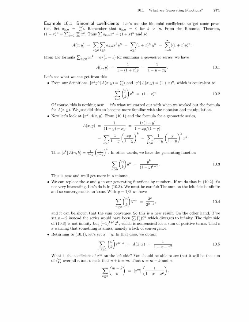
Example 10.1 Binomial coefficients Let’s use the binomial coefficients to get some prac-tice. Set ak,n =
(
nk
)
. Remember that ak,n = 0 for k > n. From the Binomial Theorem,
(1 + x)n =∑n
k=0
(
nk
)
xk. Thus∑
ak,nxk = (1 + x)n and so
A(x, y) =∑
n≥0
∑
k≥0
ak,nxkyn =∑
n≥0
(1 + x)n yn =
∞∑
n=0
((1 + x)y)n.
From the formula∑
k≥0 azk = a/(1 − z) for summing a geometric series, we have
A(x, y) =1
1 − (1 + x)y=
1
1 − y − xy. 10.1
Let’s see what we can get from this.
• From our definitions, [xkyn] A(x, y) =(
nk
)
and [yn] A(x, y) = (1 + x)n, which is equivalent to
n∑
k=0
(
n
k
)
xk = (1 + x)n 10.2
Of course, this is nothing new — it’s what we started out with when we worked out the formulafor A(x, y). We just did this to become more familiar with the notation and manipulation.
• Now let’s look at [xk] A(x, y). From (10.1) and the formula for a geometric series,
A(x, y) =1
(1 − y) − xy=
1/(1 − y)
1 − xy/(1 − y)
=∑
k≥0
1
1 − y
(
xy
1 − y
)k
=∑
k≥0
1
1 − y
(
y
1 − y
)k
xk.
Thus [xk] A(n, k) = 11−y
(
y1−y
)k
. In other words, we have the generating function
∑
n≥0
(
n
k
)
yn =yk
(1 − y)k+1. 10.3
This is new and we’ll get more in a minute.
• We can replace the x and y in our generating functions by numbers. If we do that in (10.2) it’snot very interesting. Let’s do it in (10.3). We must be careful: The sum on the left side is infiniteand so convergence is an issue. With y = 1/3 we have
∑
n≥0
(
n
k
)
3−n =3k
2k+1, 10.4
and it can be shown that the sum converges. So this is a new result. On the other hand, if weset y = 2 instead the series would have been
∑(
nk
)
2n which diverges to infinity. The right side
of (10.3) is not infinity but (−1)k+12k, which is nonsensical for a sum of positive terms. That’sa warning that something is amiss, namely a lack of convergence.
• Returning to (10.1), let’s set x = y. In that case, we obtain
∑
n,k≥0
(
n
k
)
xn+k = A(x, x) =1
1 − x − x2. 10.5
What is the coefficient of xm on the left side? You should be able to see that it will be the sumof(
nk
)
over all n and k such that n + k = m. Thus n = m − k and so
∑
k≥0
(
m − k
k
)
= [xm]
(
1
1 − x − x2
)
.
272 Chapter 10 Ordinary Generating Functions
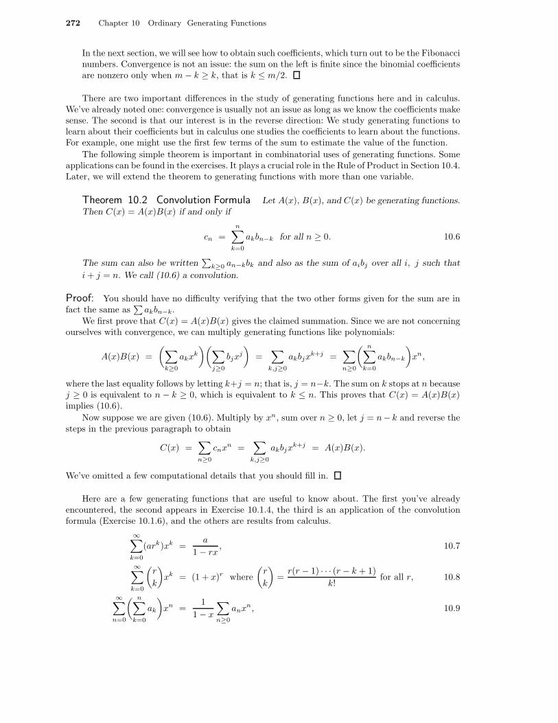
In the next section, we will see how to obtain such coefficients, which turn out to be the Fibonaccinumbers. Convergence is not an issue: the sum on the left is finite since the binomial coefficientsare nonzero only when m − k ≥ k, that is k ≤ m/2.
There are two important differences in the study of generating functions here and in calculus.We’ve already noted one: convergence is usually not an issue as long as we know the coefficients makesense. The second is that our interest is in the reverse direction: We study generating functions tolearn about their coefficients but in calculus one studies the coefficients to learn about the functions.For example, one might use the first few terms of the sum to estimate the value of the function.
The following simple theorem is important in combinatorial uses of generating functions. Someapplications can be found in the exercises. It plays a crucial role in the Rule of Product in Section 10.4.Later, we will extend the theorem to generating functions with more than one variable.
Theorem 10.2 Convolution Formula Let A(x), B(x), and C(x) be generating functions.Then C(x) = A(x)B(x) if and only if
cn =
n∑
k=0
akbn−k for all n ≥ 0. 10.6
The sum can also be written∑
k≥0 an−kbk and also as the sum of aibj over all i, j such that
i + j = n. We call (10.6) a convolution.
Proof: You should have no difficulty verifying that the two other forms given for the sum are infact the same as
∑
akbn−k.
We first prove that C(x) = A(x)B(x) gives the claimed summation. Since we are not concerningourselves with convergence, we can multiply generating functions like polynomials:
A(x)B(x) =
(
∑
k≥0
akxk
)(
∑
j≥0
bjxj
)
=∑
k,j≥0
akbjxk+j =
∑
n≥0
( n∑
k=0
akbn−k
)
xn,
where the last equality follows by letting k+j = n; that is, j = n−k. The sum on k stops at n becausej ≥ 0 is equivalent to n − k ≥ 0, which is equivalent to k ≤ n. This proves that C(x) = A(x)B(x)implies (10.6).
Now suppose we are given (10.6). Multiply by xn, sum over n ≥ 0, let j = n− k and reverse thesteps in the previous paragraph to obtain
C(x) =∑
n≥0
cnxn =∑
k,j≥0
akbjxk+j = A(x)B(x).
We’ve omitted a few computational details that you should fill in.
Here are a few generating functions that are useful to know about. The first you’ve alreadyencountered, the second appears in Exercise 10.1.4, the third is an application of the convolutionformula (Exercise 10.1.6), and the others are results from calculus.
∞∑
k=0
(ark)xk =a
1 − rx, 10.7
∞∑
k=0
(
r
k
)
xk = (1 + x)r where
(
r
k
)
=r(r − 1) · · · (r − k + 1)
k!for all r, 10.8
∞∑
n=0
( n∑
k=0
ak
)
xn =1
1 − x
∑
n≥0
anxn, 10.9

10.1 What are Generating Functions? 273
∞∑
k=0
akxk
k!= eax, 10.10
∞∑
k=1
akxk
k= − ln(1 − ax). 10.11
Exercises
These exercises will give you some practice manipulating generating functions.
10.1.1. Let p = 1 + x + x2 + x3, q = 1 + x + x2 + x3 + x4, and r = 11−x .
(a) Find the coefficient of x3 in p2; in p3; in p4.
(b) Find the coefficient of x3 in q2; in q3; in q4.
(c) Find the coefficient of x3 in r2; in r3; in r4.
(d) Can you offer a simple explanation for the fact that p, q and r all gave the same answers?
(e) Repeat (a)–(c), this time finding the coefficient of x4. Explain why some are equal and some arenot.
10.1.2. Find the coefficient of x2 in each of the following.
(a) (2 + x + x2)(1 + 2x + x2)(1 + x + 2x2)
(b) (2 + x + x2)(1 + 2x + x2)2(1 + x + 2x2)3
(c) x(1 + x)43(2 − x)5
10.1.3. Find the coefficient of x21 in (x2 + x3 + x4 + x5 + x6)8.Hint. If you are clever, you can do this without a lot of calculation.
10.1.4. This exercise explores the general binomial theorem, geometric series and related topics. Part (a)requires calculus.
(a) Let r be any real number. Use Taylor’s Theorem without worrying about convergence to prove
(1 + z)r =∑
k≥0
(
r
k
)
zk where
(
r
k
)
=r(r − 1) · · · (r − k + 1)
k!.
If you’re familiar with some form of Taylor’s Theorem with remainder, use it to show that, forsome C > 0, the infinite sum converges when |z| < C. (The largest possible value is C = 1, butyou may find it easier to use a smaller value.)
(b) Use the previous result to obtain the geometric series formula:∑
k≥0 azk = a/(1 − z).
(c) Show that∑n
k=0 azk = (a − azn+1)/(1 − z).
(d) Find a simple formula for the coefficient of xn in (1 − ax)−2.
10.1.5. In this exercise we’ll explore the effect of derivatives. Let A(x) =∑∞
m=0 amxm, the ordinarygenerating function for the sequence a. In each case, first answer the question for k = 1 and k = 2and then for general k.
(a) What is [xn] (xkA(x)), that is, the coefficient of xn in xkA(x)?
(b) Show that [xn](
d
dx
)k
A(x) =(n + k)! an+k
n!. This notation means compute the kth derivative
of A(x) and then find the coefficient of xn in the generating function. It can also be written
[xn] A(k)(x).
(c) Show that [xn](
xd
dx
)k
A(x) = nkan. This notation means that you repeat alternately the
operations of differentiating and multiplying by x a total of k times each. For example, whenk = 2 we have x(xA′(x))′.
274 Chapter 10 Ordinary Generating Functions
10.1.6. Using Theorem 10.2 or otherwise, do the following.
(a) Prove: If cn = a0 + a1 + · · · + an, then C(x) = A(x)/(1− x).
(b) Simplify(
n0
)
−(
n1
)
+ · · · + (−1)k(
nk
)
when n > 0.
(c) Suppose that dn is the sum of aibjck over all i, j, k ≥ 0 such that i + j + k = n. Express D(x)
in terms of A(x), B(x), and C(x).
10.1.7. Suppose that |r| < 1. Obtain a formula for∑
n≥0
(
nk
)
rn as a function of k and r. Show that the
sum converges by using the ratio test for series.
10.1.8. Note that (1 + x)m+n = (1 + x)m(1 + x)n. Note that the coefficients of powers of x in (1 + x)m+n,
(1+x)m, and (1+x)n are binomial coefficients. Use Theorem 10.2 to prove Vandermonde’s formula:
(
m + n
k
)
=
k∑
i=0
(
m
i
)(
n
k − i
)
.
This is one of the many identities that are known for binomial coefficients.Hint. Remember that n and k in (10.6) can be replaced by other variables. Look at the index andlimits on the summation.
10.1.9. Find a simple expression for∑
i(−1)i(
mi
)(
mk−i
)
, where the sum is over all values of i for which the
binomial coefficients in the sum are defined.
10.1.10. The results given here are referred to as bisection of series. Let A(x) =∑∞
n=0 anxn.
(a) Show that (A(x) + A(−x))/2 is the generating function for the sequence bn which is zero forodd n and equals an for even n.
(b) What is the generating function for the sequence cn which is zero for even n and equals an forodd n?
(c) Evaluate∑
k≥0
(
n2k
)
x2k where x is a real number. In particular, what is∑
k≥0
(
n2k
)
?
*10.1.11. Fix k > 1 and 0 ≤ j < k. If you are familiar with kth roots of unity, generalize the Exercise 10.1.10to the sequence bn which is an when n + j is a multiple of k and is zero otherwise:
B(x) =1
k
k−1∑
s=0
ωjsA(ωsx),
where ω = exp(2πi/k), a primitive kth root of unity. (The result is called multisection of series.)
10.1.12. Evaluate sk =
∞∑
n=0
(
2n
k
)
2−n.
*10.1.13. Using Exercise 10.1.11, show that
∞∑
n=0
x3n
(3n)!=
ex
3+
2 cos(x√
3/2)
3ex/2
and develop similar formulas for∑
p3n+1/(3n + 1)! and∑
p3n+2/(3n + 2)!.
10.2 Solving a Single Recursion 275
*10.1.14. We use the terminology from the Principle of Inclusion and Exclusion (Theorem 4.1 (p. 95)). Also,let Ek be the number of elements of S that lie in exactly k of the sets S1, S2, . . . , Sm.
(a) Using the Rules of Sum and Product (not Theorem 4.1), prove that
Nr =∑
k≥0
(
r + k
r
)
Er+k.
(b) If the generating functions corresponding to E0, E1, . . . and N0, N1, . . . are E(x) and N(x),conclude that N(x) = E(x + 1).
(c) Use this to conclude that E(x) = N(x − 1) and then deduce the extension of the Principle ofInclusion and Exclusion:
Ek =∑
i≥0
(−1)i(
k + i
i
)
Nk+i.
10.2 Solving a Single Recursion
In this section we’ll use ordinary generating functions to solve some simple recursions, including twothat we were unable to solve previously: the Fibonacci numbers and the number of unlabeled fullbinary RP-trees.
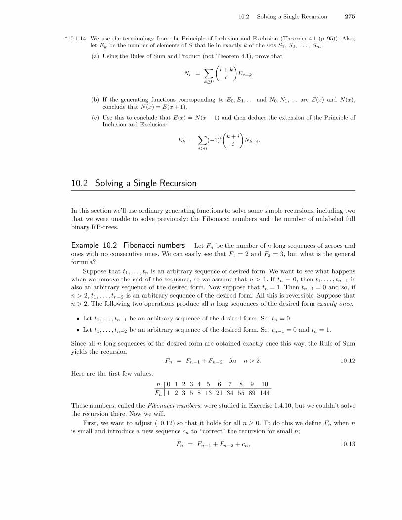
Example 10.2 Fibonacci numbers Let Fn be the number of n long sequences of zeroes andones with no consecutive ones. We can easily see that F1 = 2 and F2 = 3, but what is the generalformula?
Suppose that t1, . . . , tn is an arbitrary sequence of desired form. We want to see what happenswhen we remove the end of the sequence, so we assume that n > 1. If tn = 0, then t1, . . . , tn−1 isalso an arbitrary sequence of the desired form. Now suppose that tn = 1. Then tn−1 = 0 and so, ifn > 2, t1, . . . , tn−2 is an arbitrary sequence of the desired form. All this is reversible: Suppose thatn > 2. The following two operations produce all n long sequences of the desired form exactly once.
• Let t1, . . . , tn−1 be an arbitrary sequence of the desired form. Set tn = 0.
• Let t1, . . . , tn−2 be an arbitrary sequence of the desired form. Set tn−1 = 0 and tn = 1.
Since all n long sequences of the desired form are obtained exactly once this way, the Rule of Sumyields the recursion
Fn = Fn−1 + Fn−2 for n > 2. 10.12
Here are the first few values.
n 0 1 2 3 4 5 6 7 8 9 10
Fn 1 2 3 5 8 13 21 34 55 89 144
These numbers, called the Fibonacci numbers, were studied in Exercise 1.4.10, but we couldn’t solvethe recursion there. Now we will.
First, we want to adjust (10.12) so that it holds for all n ≥ 0. To do this we define Fn when nis small and introduce a new sequence cn to “correct” the recursion for small n;
Fn = Fn−1 + Fn−2 + cn, 10.13
276 Chapter 10 Ordinary Generating Functions
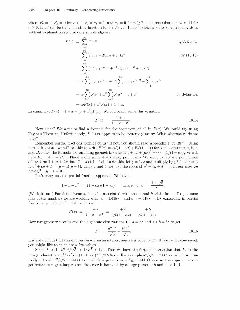
where F0 = 1, Fk = 0 for k < 0, c0 = c1 = 1, and cn = 0 for n ≥ 2. This recursion is now valid forn ≥ 0. Let F (x) be the generating function for F0, F1, . . .. In the following series of equations, stepswithout explanation require only simple algebra.
F (x) =∞∑
n=0
Fnxn by defintion
=
∞∑
n=0
(Fn−1 + Fn−2 + cn)xn by (10.13)
=
∞∑
n=0
(
xFn−1xn−1 + x2Fn−2x
n−2 + cnxn)
= x∞∑
n=0
Fn−1xn−1 + x2
∞∑
n=0
Fn−2xn−2 +
∞∑
n=0
anxn
= x
∞∑
i=1
Fixi + x2
∞∑
k=0
Fkxk + 1 + x by definition
= xF (x) + x2F (x) + 1 + x.
In summary, F (x) = 1 + x + (x + x2)F (x). We can easily solve this equation:
F (x) =1 + x
1 − x − x2. 10.14
Now what? We want to find a formula for the coefficient of xn in F (x). We could try using
Taylor’s Theorem. Unfortunately, F (n)(x) appears to be extremely messy. What alternative do wehave?
Remember partial fractions from calculus? If not, you should read Appendix D (p. 387). Usingpartial fractions, we will be able to write F (x) = A/(1− ax)+B/(1− bx) for some constants a, b, Aand B. Since the formula for summing geometric series is 1 + ax + (ax)2 + · · · = 1/(1− ax), we willhave Fn = Aan + Bbn. There is one somewhat sneaky point here. We want to factor a polynomialof the form 1+ cx+dx2 into (1−ax)(1− bx). To do this, let y = 1/x and multiply by y2. The resultis y2 + cy + d = (y − a)(y − b). Thus a and b are just the roots of y2 + cy + d = 0. In our case wehave y2 − y − 1 = 0.
Let’s carry out the partial fraction approach. We have
1 − x − x2 = (1 − ax)(1 − bx) where a, b =1 ±
√5
2.
(Work it out.) For definitiveness, let a be associated with the + and b with the −. To get someidea of the numbers we are working with, a = 1.618 · · · and b = −.618 · · · . By expanding in partialfractions, you should be able to derive
F (x) =1 + x
1 − x − x2=
1 + a√5(1 − ax)
− 1 + b√5(1 − bx)
.
Now use geometric series and the algebraic observations 1 + a = a2 and 1 + b = b2 to get
Fn =an+2
√5
− bn+2
√5
. 10.15
It is not obvious that this expression is even an integer, much less equal to Fn. If you’re not convinced,you might like to calculate a few values.
Since |b| < 1,∣
∣bn+2/√
5∣
∣ < 1/√
5 < 1/2. Thus we have the further observation that Fn is the
integer closest to an+2/√
5 = (1.618 · · ·)n+2/2.236 · · ·. For example a4/√
5 = 3.065 · · · which is close
to F2 = 3 and a12/√
5 = 144.001 · · ·, which is quite close to F10 = 144. Of course, the approximationsget better as n gets larger since the error is bounded by a large power of b and |b| < 1.
10.2 Solving a Single Recursion 277
The method that we have just used works for many other recursions, so it is useful to lay it out
as a series of steps. Although our description is for a singly indexed recursion, it can be applied to
the multiply indexed case as well.
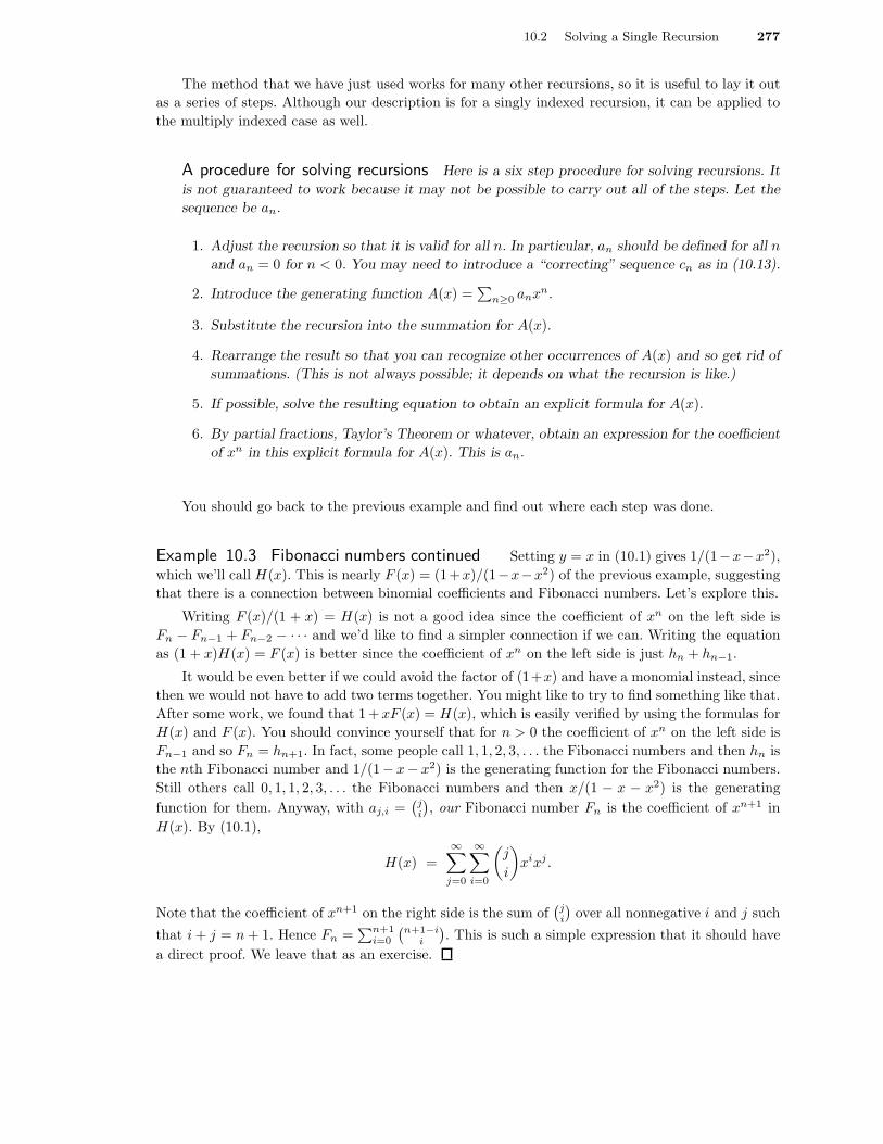
A procedure for solving recursions Here is a six step procedure for solving recursions. It
is not guaranteed to work because it may not be possible to carry out all of the steps. Let the
sequence be an.
1. Adjust the recursion so that it is valid for all n. In particular, an should be defined for all n
and an = 0 for n < 0. You may need to introduce a “correcting” sequence cn as in (10.13).
2. Introduce the generating function A(x) =∑
n≥0 anxn.
3. Substitute the recursion into the summation for A(x).
4. Rearrange the result so that you can recognize other occurrences of A(x) and so get rid of
summations. (This is not always possible; it depends on what the recursion is like.)
5. If possible, solve the resulting equation to obtain an explicit formula for A(x).
6. By partial fractions, Taylor’s Theorem or whatever, obtain an expression for the coefficient
of xn in this explicit formula for A(x). This is an.
You should go back to the previous example and find out where each step was done.
Example 10.3 Fibonacci numbers continued Setting y = x in (10.1) gives 1/(1−x−x2),
which we’ll call H(x). This is nearly F (x) = (1+x)/(1−x−x2) of the previous example, suggesting
that there is a connection between binomial coefficients and Fibonacci numbers. Let’s explore this.
Writing F (x)/(1 + x) = H(x) is not a good idea since the coefficient of xn on the left side is
Fn − Fn−1 + Fn−2 − · · · and we’d like to find a simpler connection if we can. Writing the equation
as (1 + x)H(x) = F (x) is better since the coefficient of xn on the left side is just hn + hn−1.
It would be even better if we could avoid the factor of (1+x) and have a monomial instead, since
then we would not have to add two terms together. You might like to try to find something like that.
After some work, we found that 1+xF (x) = H(x), which is easily verified by using the formulas for
H(x) and F (x). You should convince yourself that for n > 0 the coefficient of xn on the left side is
Fn−1 and so Fn = hn+1. In fact, some people call 1, 1, 2, 3, . . . the Fibonacci numbers and then hn is
the nth Fibonacci number and 1/(1− x− x2) is the generating function for the Fibonacci numbers.
Still others call 0, 1, 1, 2, 3, . . . the Fibonacci numbers and then x/(1 − x − x2) is the generating
function for them. Anyway, with aj,i =(
ji
)
, our Fibonacci number Fn is the coefficient of xn+1 in
H(x). By (10.1),
H(x) =
∞∑
j=0
∞∑
i=0
(
j
i
)
xixj .
Note that the coefficient of xn+1 on the right side is the sum of(
ji
)
over all nonnegative i and j such
that i + j = n + 1. Hence Fn =∑n+1
i=0
(
n+1−ii
)
. This is such a simple expression that it should have
a direct proof. We leave that as an exercise.
278 Chapter 10 Ordinary Generating Functions
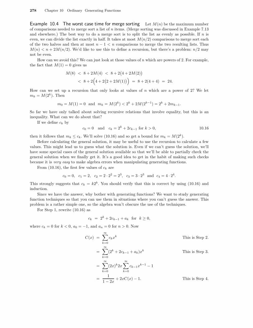
Example 10.4 The worst case time for merge sorting Let M(n) be the maximum numberof comparisons needed to merge sort a list of n items. (Merge sorting was discussed in Example 7.13and elsewhere.) The best way to do a merge sort is to split the list as evenly as possible. If n iseven, we can divide the list exactly in half. It takes at most M(n/2) comparisons to merge sort eachof the two halves and then at most n − 1 < n comparisons to merge the two resulting lists. ThusM(n) < n + 2M(n/2). We’d like to use this to define a recursion, but there’s a problem: n/2 maynot be even.
How can we avoid this? We can just look at those values of n which are powers of 2. For example,the fact that M(1) = 0 gives us
M(8) < 8 + 2M(4) < 8 + 2(
4 + 2M(2))
< 8 + 2(
4 + 2(
2 + 2M(1))
)
= 8 + 2(4 + 4) = 24.
How can we set up a recursion that only looks at values of n which are a power of 2? We letmk = M(2k). Then
m0 = M(1) = 0 and mk = M(2k) < 2k + 2M(2k−1) = 2k + 2mk−1.
So far we have only talked about solving recursive relations that involve equality, but this is aninequality. What can we do about that?
If we define ck by
c0 = 0 and ck = 2k + 2ck−1 for k > 0, 10.16
then it follows that mk ≤ ck. We’ll solve (10.16) and so get a bound for mk = M(2k).
Before calculating the general solution, it may be useful to use the recursion to calculate a fewvalues. This might lead us to guess what the solution is. Even if we can’t guess the solution, we’llhave some special cases of the general solution available so that we’ll be able to partially check thegeneral solution when we finally get it. It’s a good idea to get in the habit of making such checksbecause it is very easy to make algebra errors when manipulating generating functions.
From (10.16), the first few values of ck are
c0 = 0, c1 = 2, c2 = 2 · 22 = 23, c3 = 3 · 23 and c4 = 4 · 24.
This strongly suggests that ck = k2k. You should verify that this is correct by using (10.16) andinduction.
Since we have the answer, why bother with generating functions? We want to study generatingfunction techniques so that you can use them in situations where you can’t guess the answer. Thisproblem is a rather simple one, so the algebra won’t obscure the use of the techniques.
For Step 1, rewrite (10.16) as
ck = 2k + 2ck−1 + ak for k ≥ 0,
where ck = 0 for k < 0, a0 = −1, and an = 0 for n > 0. Now
C(x) =
∞∑
k=0
ckxk This is Step 2.
=
∞∑
k=0
(2k + 2ck−1 + ak)xk This is Step 3.
=
∞∑
k=0
(2x)k2x
∞∑
k=0
ck−1xk−1 − 1
=1
1 − 2x+ 2xC(x) − 1. This is Step 4.
10.2 Solving a Single Recursion 279
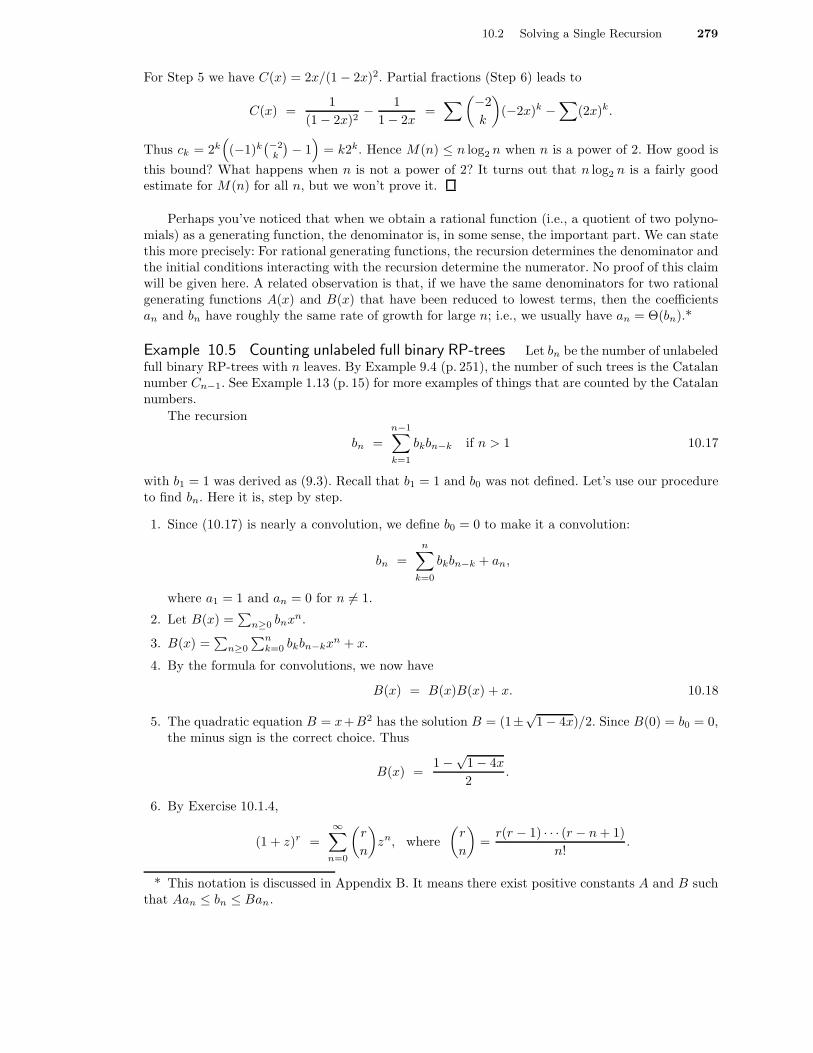
For Step 5 we have C(x) = 2x/(1 − 2x)2. Partial fractions (Step 6) leads to
C(x) =1
(1 − 2x)2− 1
1 − 2x=∑
(−2
k
)
(−2x)k −∑
(2x)k.
Thus ck = 2k(
(−1)k(−2
k
)
− 1)
= k2k. Hence M(n) ≤ n log2 n when n is a power of 2. How good is
this bound? What happens when n is not a power of 2? It turns out that n log2 n is a fairly goodestimate for M(n) for all n, but we won’t prove it.
Perhaps you’ve noticed that when we obtain a rational function (i.e., a quotient of two polyno-mials) as a generating function, the denominator is, in some sense, the important part. We can statethis more precisely: For rational generating functions, the recursion determines the denominator andthe initial conditions interacting with the recursion determine the numerator. No proof of this claimwill be given here. A related observation is that, if we have the same denominators for two rationalgenerating functions A(x) and B(x) that have been reduced to lowest terms, then the coefficientsan and bn have roughly the same rate of growth for large n; i.e., we usually have an = Θ(bn).*
Example 10.5 Counting unlabeled full binary RP-trees Let bn be the number of unlabeledfull binary RP-trees with n leaves. By Example 9.4 (p. 251), the number of such trees is the Catalannumber Cn−1. See Example 1.13 (p. 15) for more examples of things that are counted by the Catalannumbers.
The recursion
bn =
n−1∑
k=1
bkbn−k if n > 1 10.17
with b1 = 1 was derived as (9.3). Recall that b1 = 1 and b0 was not defined. Let’s use our procedureto find bn. Here it is, step by step.
1. Since (10.17) is nearly a convolution, we define b0 = 0 to make it a convolution:
bn =
n∑
k=0
bkbn−k + an,
where a1 = 1 and an = 0 for n 6= 1.
2. Let B(x) =∑
n≥0 bnxn.
3. B(x) =∑
n≥0
∑nk=0 bkbn−kxn + x.
4. By the formula for convolutions, we now have
B(x) = B(x)B(x) + x. 10.18
5. The quadratic equation B = x+B2 has the solution B = (1±√
1 − 4x)/2. Since B(0) = b0 = 0,the minus sign is the correct choice. Thus
B(x) =1 −
√1 − 4x
2.
6. By Exercise 10.1.4,
(1 + z)r =
∞∑
n=0
(
r
n
)
zn, where
(
r
n
)
=r(r − 1) · · · (r − n + 1)
n!.
* This notation is discussed in Appendix B. It means there exist positive constants A and B suchthat Aan ≤ bn ≤ Ban.
280 Chapter 10 Ordinary Generating Functions
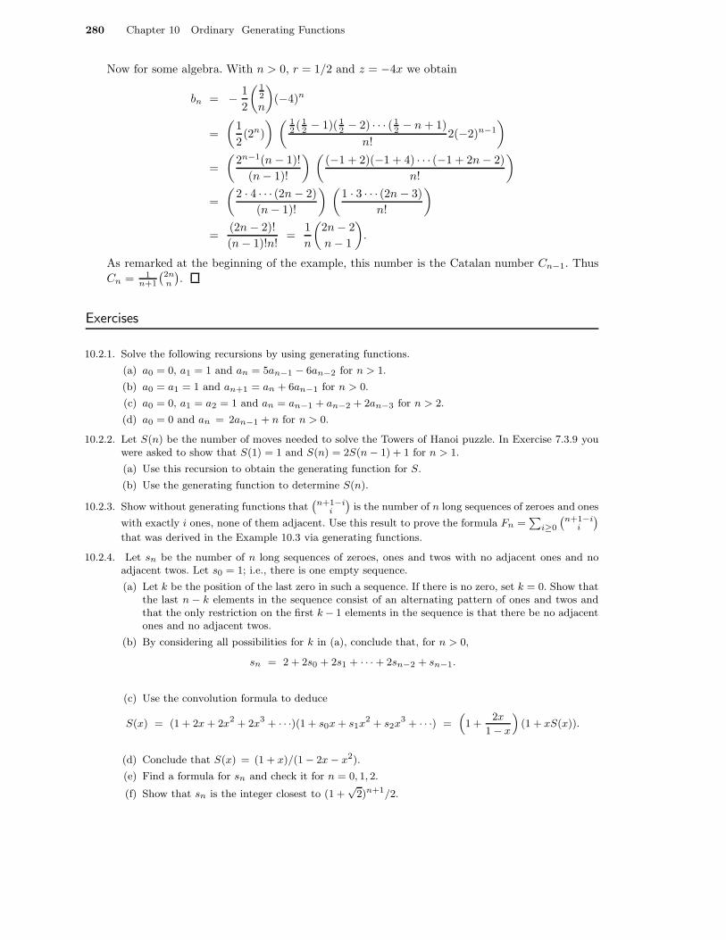
Now for some algebra. With n > 0, r = 1/2 and z = −4x we obtain
bn = − 1
2
(12
n
)
(−4)n
=
(
1
2(2n)
) ( 12 (1
2 − 1)(12 − 2) · · · (1
2 − n + 1)
n!2(−2)n−1
)
=
(
2n−1(n − 1)!
(n − 1)!
) (
(−1 + 2)(−1 + 4) · · · (−1 + 2n − 2)
n!
)
=
(
2 · 4 · · · (2n − 2)
(n − 1)!
) (
1 · 3 · · · (2n − 3)
n!
)
=(2n − 2)!
(n − 1)!n!=
1
n
(
2n − 2
n − 1
)
.
As remarked at the beginning of the example, this number is the Catalan number Cn−1. Thus
Cn = 1n+1
(
2nn
)
.
Exercises
10.2.1. Solve the following recursions by using generating functions.
(a) a0 = 0, a1 = 1 and an = 5an−1 − 6an−2 for n > 1.
(b) a0 = a1 = 1 and an+1 = an + 6an−1 for n > 0.
(c) a0 = 0, a1 = a2 = 1 and an = an−1 + an−2 + 2an−3 for n > 2.
(d) a0 = 0 and an = 2an−1 + n for n > 0.
10.2.2. Let S(n) be the number of moves needed to solve the Towers of Hanoi puzzle. In Exercise 7.3.9 youwere asked to show that S(1) = 1 and S(n) = 2S(n − 1) + 1 for n > 1.
(a) Use this recursion to obtain the generating function for S.
(b) Use the generating function to determine S(n).
10.2.3. Show without generating functions that(
n+1−ii
)
is the number of n long sequences of zeroes and ones
with exactly i ones, none of them adjacent. Use this result to prove the formula Fn =∑
i≥0
(
n+1−ii
)
that was derived in the Example 10.3 via generating functions.
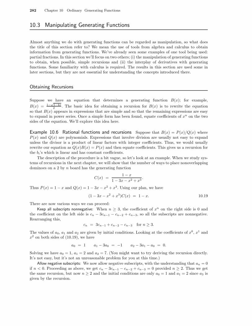
10.2.4. Let sn be the number of n long sequences of zeroes, ones and twos with no adjacent ones and noadjacent twos. Let s0 = 1; i.e., there is one empty sequence.
(a) Let k be the position of the last zero in such a sequence. If there is no zero, set k = 0. Show thatthe last n − k elements in the sequence consist of an alternating pattern of ones and twos andthat the only restriction on the first k − 1 elements in the sequence is that there be no adjacentones and no adjacent twos.
(b) By considering all possibilities for k in (a), conclude that, for n > 0,
sn = 2 + 2s0 + 2s1 + · · · + 2sn−2 + sn−1.
(c) Use the convolution formula to deduce
S(x) = (1 + 2x + 2x2 + 2x3 + · · ·)(1 + s0x + s1x2 + s2x3 + · · ·) =(
1 +2x
1 − x
)
(1 + xS(x)).
(d) Conclude that S(x) = (1 + x)/(1 − 2x − x2).
(e) Find a formula for sn and check it for n = 0, 1, 2.
(f) Show that sn is the integer closest to (1 +√
2)n+1/2.

10.2 Solving a Single Recursion 281
10.2.5. The usual method for multiplying two polynomials of degree n − 1, say
P1(x) = a0,1 + a1,1x + · · · + an−1,1xn−1 and P2(x) = a0,2 + a1,2x + · · · + an−1,2xn−1
requires n2 multiplications to form the products ai,1aj,2 for 0 ≤ i, j < n. These are added togetherin the appropriate way to form the 2n − 1 sums that constitute the coefficients of the productP1(x)P2(x). There is a less direct method that requires less multiplications. For simplicity, supposethat n = 2m.
• First, split the polynomials in “half”: Pi(x) = Li(x) + xmHi(x), where Li and Hi havedegree at most m − 1.
• Second, let A = H1H2, B = L1L2 and C = (H1 + L1)(H2 + L2).
• Third, note that P1P2 = Ax2m + B + (C − A − B)xm.
(a) Prove that the formula for P1P2 is correct.
(b) Let M(n) be the least number of multiplications we need in a general purpose algorithm formultiplying two polynomials of degree n − 1. show that M(2m) ≤ 3M(m).
(c) Use the previous result to derive an upper bound for M(n) when n is a power of 2 that is better
than n2. (Your answer should be M(n) ≤ nc where c = 1.58 · · ·.) How does this bound compare
with n2 when n = 210 = 1024?Your bound will give a bound for all n since, if n ≤ 2k , we can fill the polynomials out to
degree 2k by introducing high degree terms with zero coefficients. This gives M(n) ≤ M(2k).
(d) Show how the method used to obtain the bound multiplies 1 + 2x − x2 + 3x3 and 5 + 2x −x3.
*(e) It may be objected that our method could lead to such a large number of additions andsubtractions that the savings in multiplication may be lost. Does this happen? Justify youranswer.
10.2.6. Let tn be the number of n-vertex unlabeled binary RP-trees. (Each vertex has 0, 1 or 2 children.)
(a) Derive the recursion
t1 = 1 and tn+1 = tn +
n−1∑
k=1
tktn−k for n > 0.
(b) With t0 = 0, derive an equation for the generating function T (x) =∑
n≥0 tnxn.
(c) Solve the equation in (b) to obtain
T (x) =1 − x −
√1 − 2x − 3x2
2x
and explain the choice of sign before the square root.
10.2.7. Let c1, . . . , ck be arbitrary real numbers. If you are familiar with partial fractions, explain why the
solution to the recursion an = c1an−1 + · · · + ckak−k has the form an =∑m
i=1 Pi(n)rni for all
sufficiently large n, where Pi(n) is a polynomial of degree less than di, the ri are all different, and
1 − c1x − · · · − ckxk =
m∏
i=1
(1 − rix)di .
How can the polynomials Pn(n) be found without using partial fractions?
282 Chapter 10 Ordinary Generating Functions
10.3 Manipulating Generating Functions
Almost anything we do with generating functions can be regarded as manipulation, so what doesthe title of this section refer to? We mean the use of tools from algebra and calculus to obtaininformation from generating functions. We’ve already seen some examples of one tool being used:partial fractions. In this section we’ll focus on two others; (i) the manipulation of generating functionsto obtain, when possible, simple recursions and (ii) the interplay of derivatives with generatingfunctions. Some familiarity with calculus is required. The results in this section are used some inlater sections, but they are not essential for understanding the concepts introduced there.
Obtaining Recursions
Suppose we have an equation that determines a generating function B(x); for example,
B(x) = 1−√
1−4x2 . The basic idea for obtaining a recursion for B(x) is to rewrite the equation
so that B(x) appears in expressions that are simple and so that the remaining expressions are easyto expand in power series. Once a simple form has been found, equate coefficients of xn on the twosides of the equation. We’ll explore this idea here.
Example 10.6 Rational functions and recursions Suppose that B(x) = P (x)/Q(x) whereP (x) and Q(x) are polynomials. Expressions that involve division are usually not easy to expandunless the divisor is a product of linear factors with integer coefficients. Thus, we would usuallyrewrite our equation as Q(x)B(x) = P (x) and then equate coefficients. This gives us a recursion forthe bi’s which is linear and has constant coefficients.
The description of the procedure is a bit vague, so let’s look at an example. When we study sys-tems of recursions in the next chapter, we will show that the number of ways to place nonoverlappingdominoes on a 2 by n board has the generating function
C(x) =1 − x
1 − 3x − x2 + x3.
Thus P (x) = 1 − x and Q(x) = 1 − 3x − x2 + x3. Using our plan, we have
(1 − 3x − x2 + x3)C(x) = 1 − x. 10.19
There are now various ways we can proceed:
Keep all subscripts nonnegative: When n ≥ 3, the coefficient of xn on the right side is 0 andthe coefficient on the left side is cn − 3cn−1 − cn−2 + cn−3, so all the subscripts are nonnegative.Rearranging this,
cn = 3cn−1 + cn−2 − cn−3 for n ≥ 3.
The values of a0, a1 and a2 are given by initial conditions. Looking at the coefficients of x0, x1 andx2 on both sides of (10.19), we have
a0 = 1 a1 − 3a0 = −1 a2 − 3a1 − a0 = 0.
Solving we have a0 = 1, a1 = 2 and a2 = 7. (You might want to try deriving the recursion directly.It’s not easy, but it’s not an unreasonable problem for you at this time.)
Allow negative subscripts: We now allow negative subscripts, with the understanding that an = 0if n < 0. Proceeding as above, we get cn − 3cn−1 − cn−2 + cn−3 = 0 provided n ≥ 2. Thus we getthe same recursion, but now n ≥ 2 and the initial conditions are only a0 = 1 and a1 = 2 since a3 isgiven by the recursion.
10.3 Manipulating Generating Functions 283
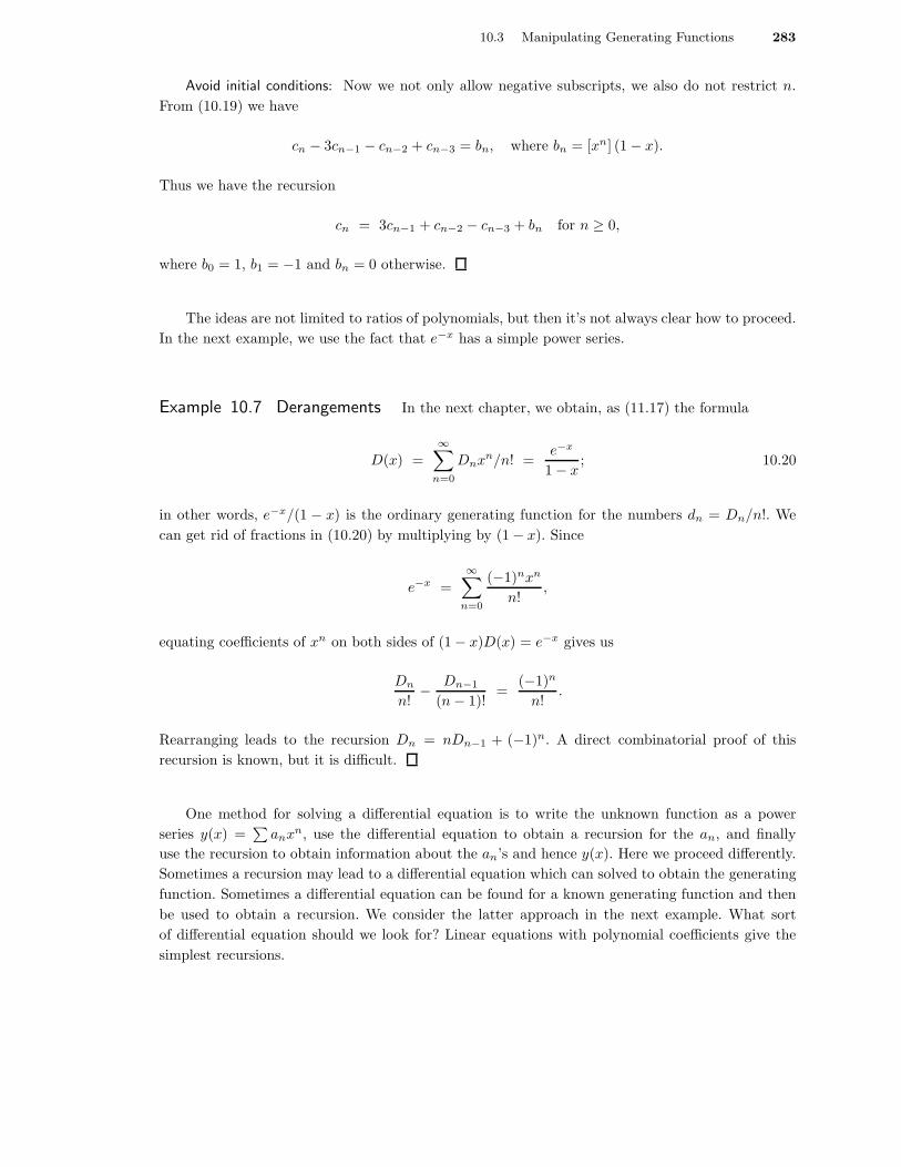
Avoid initial conditions: Now we not only allow negative subscripts, we also do not restrict n.
From (10.19) we have
cn − 3cn−1 − cn−2 + cn−3 = bn, where bn = [xn] (1 − x).
Thus we have the recursion
cn = 3cn−1 + cn−2 − cn−3 + bn for n ≥ 0,
where b0 = 1, b1 = −1 and bn = 0 otherwise.
The ideas are not limited to ratios of polynomials, but then it’s not always clear how to proceed.
In the next example, we use the fact that e−x has a simple power series.
Example 10.7 Derangements In the next chapter, we obtain, as (11.17) the formula
D(x) =∞∑
n=0
Dnxn/n! =e−x
1 − x; 10.20
in other words, e−x/(1 − x) is the ordinary generating function for the numbers dn = Dn/n!. We
can get rid of fractions in (10.20) by multiplying by (1 − x). Since
e−x =
∞∑
n=0
(−1)nxn
n!,
equating coefficients of xn on both sides of (1 − x)D(x) = e−x gives us
Dn
n!− Dn−1
(n − 1)!=
(−1)n
n!.
Rearranging leads to the recursion Dn = nDn−1 + (−1)n. A direct combinatorial proof of this
recursion is known, but it is difficult.
One method for solving a differential equation is to write the unknown function as a power
series y(x) =∑
anxn, use the differential equation to obtain a recursion for the an, and finally
use the recursion to obtain information about the an’s and hence y(x). Here we proceed differently.
Sometimes a recursion may lead to a differential equation which can solved to obtain the generating
function. Sometimes a differential equation can be found for a known generating function and then
be used to obtain a recursion. We consider the latter approach in the next example. What sort
of differential equation should we look for? Linear equations with polynomial coefficients give the
simplest recursions.

284 Chapter 10 Ordinary Generating Functions
Example 10.8 A recursion for unlabeled full binary RP-trees In Example 10.5 we found
that the generating function for unlabeled full binary RP-trees is B(x) = 1−√
1−4x2 . We then obtained
an explicit formula for bn by expanding√
1 − 4x in a power series. Instead, we could obtain adifferential equation which would lead to a recursion.
We can proceed in various ways to obtain a simple differential equation. One is to observe that
2B(x) − 1 = −(1 − 4x)1/2 and differentiate both sides to obtain 2B′(x) = 2(1 − 4x)−1/2. Multiplyby 1 − 4x:
2(1 − 4x)B′(x) = 2(1 − 4x)1/2 = −(2B(x) − 1).
Thus 2B′(x) − 8xB′(x) + 2B(x) = 1. Replacing B(x) by its power series we obtain∑
2nbnxn−1 −∑
8nbnxn +∑
2bnxn = 1.
Replacing the first sum by∑
2(n + 1)bn+1xn and equating coefficients of xn gives
2(n + 1)bn+1 − 8nbn + 2bn = 0 for n > 0.
After some rearrangement, bn+1 = (4n−2)bn/(n+1) for n > 0. We already know that b1 = 1, so wehave the initial condition for the recursion. This recursion was obtained in Exercise 9.3.13 (p. 266)by a counting argument.
Derivatives, Averages and Probability
The fact that xA′(x) =∑
nanxn can be quite useful in obtaining information about averages. We’llexplain how this works and then look at some examples.
Let An be a set of objects of size n; for example, some kind of n-long sequences or some kind ofn-vertex trees. For each n, make An into a probability space using the uniform distribution:
Pr(α) =1
|An|for all α ∈ An.
(Probability is discussed in Appendix C.) Suppose that for each n we have a random variable Xn onAn that counts something; for example, the number of ones in a sequence or the number of leaveson a tree. The average value (average number of ones or average number of leaves) is then E(Xn).
Now let’s look at this in generating function terms. Let an,k be the number of α ∈ An withXn(α) = k; for example, the number of n-long sequences with k ones or the number of n-vertex trees
with k leaves. Let A(x, y) be the generating function∑
n,k an,kxnyk. By the definition of expectation
and simple algebra,
E(Xn) =∑
k
k Pr(Xn =k) =∑
k
kan,k
|An|=
∑
k kan,k
|An|=
∑
k kan,k∑
k an,k.
Let’s look at the two sums in the last fraction.
Since [xn] A(x, y) =∑
k an,kyk,∑
k an,k = [xn]A(x, 1).
Since [xn] ∂A(x,y)∂y =
∑
k kan,kyk−1,∑
k kan,k = [xn]Ay(x, 1),
where Ay stands for ∂A/∂y. Putting this all together,
E(Xn) =[xn] Ay(x, 1)
[xn] A(x, 1). 10.21
We can use the same idea to compute variance. Recall that var(Xn) = E(X2n)−E(Xn)2. Since
(10.21) tells us how to compute E(Xn), all we need is a formula for E(X2n). This is just like the

10.3 Manipulating Generating Functions 285
previous derivation except we need factors of k2 multiplying an,k. We can get this by differentiating
twice:∑
k
k2an,k = [xn]∂(yAy(x, y))
∂y
∣
∣
∣
∣
y=1
= [xn](Ayy(x, 1) + Ay(x, 1)). 10.22
This discussion has all been rather abstract. Let’s apply it.
Example 10.9 Fibonacci sequences What is the average number of ones in an n long sequence
of zeroes and ones containing no adjacent ones? We studied these sequences in Example 10.2 (p. 275),
where we used the notation Fn. To be more in keeping with the previous discussion, let Let fn,k be
the number of n long sequences containing exactly k ones. We need F (x, y) =∑
n,k fn,kxnyk.
In Example 10.16 we’ll see how to compute F (x, y) quickly, but for now the only tool we have
is recursions, so it will take a bit longer. You should be able to extend the argument used to derive
the recursion (10.12) to show that
fn,k = fn−1,k + fn−2,k−1 for n ≥ 2, 10.23
provided we set fn,k = 0 when k < 0. Let Fn(y) =∑
k fn,kyk and sum yk times (10.23) over all k
to obtain
Fn(y) = Fn−1(y) + yFn−2(y) for n ≥ 2. 10.24
For n = 0 we have only the empty sequence and for n = 1 we have the two sequences 0 and 1. Thus,
the initial conditions for (10.24) are F0(y) = 1 and F1(y) = 1 + y. Multiplying (10.24) by xn and
summing over n ≥ 2, we obtain
F (x, y) − F0(y) − xF1(y) = x(
F (x, y) − F0(y))
+ x2yF (x, y).
Thus
F (x, y) =1 + xy
1 − x − x2y. 10.25
We are now ready to use (10.21). From (10.25),
Fy(x, y) =x(1 − x − x2y) − (1 + xy)(−x2)
(1 − x − x2y)2=
x
(1 − x − x2y)2
and so
Fy(x, 1) =x
(1 − x − x2)2.
Thus
[xn] Fy(x, 1) = [xn−1]1
(1 − x − x2)2.
This can be expanded by partial fractions in various ways. The easiest method is probably to use
the ideas and formulas in Appendix D (p. 387), which we now do. With a, b = (1 ±√
5)/2, as in
Example 10.2, we have
1
(1 − x − x2)2=
1
(1 − ax)2(1 − bx)2.
We make use of the relations
a + b = 1 ab = −1 and a − b =√
5.

286 Chapter 10 Ordinary Generating Functions
Here are the calculations
1
(1 − ax)2(1 − bx)2=
(
a/√
5
1 − ax− b/
√5
1 − bx
)2
=a2/5
(1 − ax)2− 2ab/5
(1 − ax)(1 − bx)+
b2/5
(1 − bx)2
=a2/5
(1 − ax)2+
2a/5√
5
1 − ax− 2b/5
√5
1 − bx+
b2/5
(1 − bx)2.
Thus
[xn] Fy(x, 1) =a2
5
( −2
n − 1
)
(−a)n−1 +2a
5√
5an−1 − 2b
5√
5bn−1 +
b2
5
( −2
n − 1
)
(−b)n−1
=nan+1
5+
2an
5√
5− 2bn
5√
5+
nbn+1
5.
Since |b| < .62, the last two terms in this expression are fairly small. In fact, we will show that wn
is the integer closest toan
5
(
an + 2/√
5)
.
Using the expression (10.15) for∑
k fn,k, the average number of ones is very close to
n
a√
5+
2
5a2.
We must prove our claim about the smallness of the terms involving b. It suffices to show that
their sum is less than 1/2. Since |b| = (√
5 − 1)/2 < 1, we have
2|b|n5√
5≤ 2b
5√
5< 0.12.
The term n|b|n+1/5 is a bit more complicated. We study it as a function of n to find its maximum.Its derivative with respect to n is
|b|n+1
5+
n ln |b| |b|n+1
5=
|b|n+1
5(1 + n ln |b|).
Since −0.25 < ln |b| < −0.2, this is positive for n ≤ 4 and negative for n ≥ 5. It follows that theterm achieves its maximum at n = 4 or at n = 5. The values of these two terms are
4|b|5/5 < |b|5 < 0.1 and 5|b|6/5 < |b|5 < 0.1,
proving our claim.
Example 10.10 Leaves in trees What can we say about the number of leaves in n-vertexunlabeled RP-trees? We’ll study the average number of leaves and the variance using (10.21) and(10.22).
Let tn,k be the number of unlabeled RP-trees having n vertices and k leaves and let T (x, y) be∑
n,k tn,kxnyk. Using tools at our disposal, it is not easy to work out the generating function for
T (x, y). On the other hand, after you have read the next section, you should be able to show that
T (x, y) = xy + xT (x, y) + x(T (x, y))2 + · · · + x(T (x, y))i + · · · ,where x(T (x, y))i comes from building trees whose roots have degree i. We’ll assume this has beendone. Summing the geometric series in (10.25), we have
T (x, y) = xy +xT (x, y)
1 − T (x, y).
10.3 Manipulating Generating Functions 287
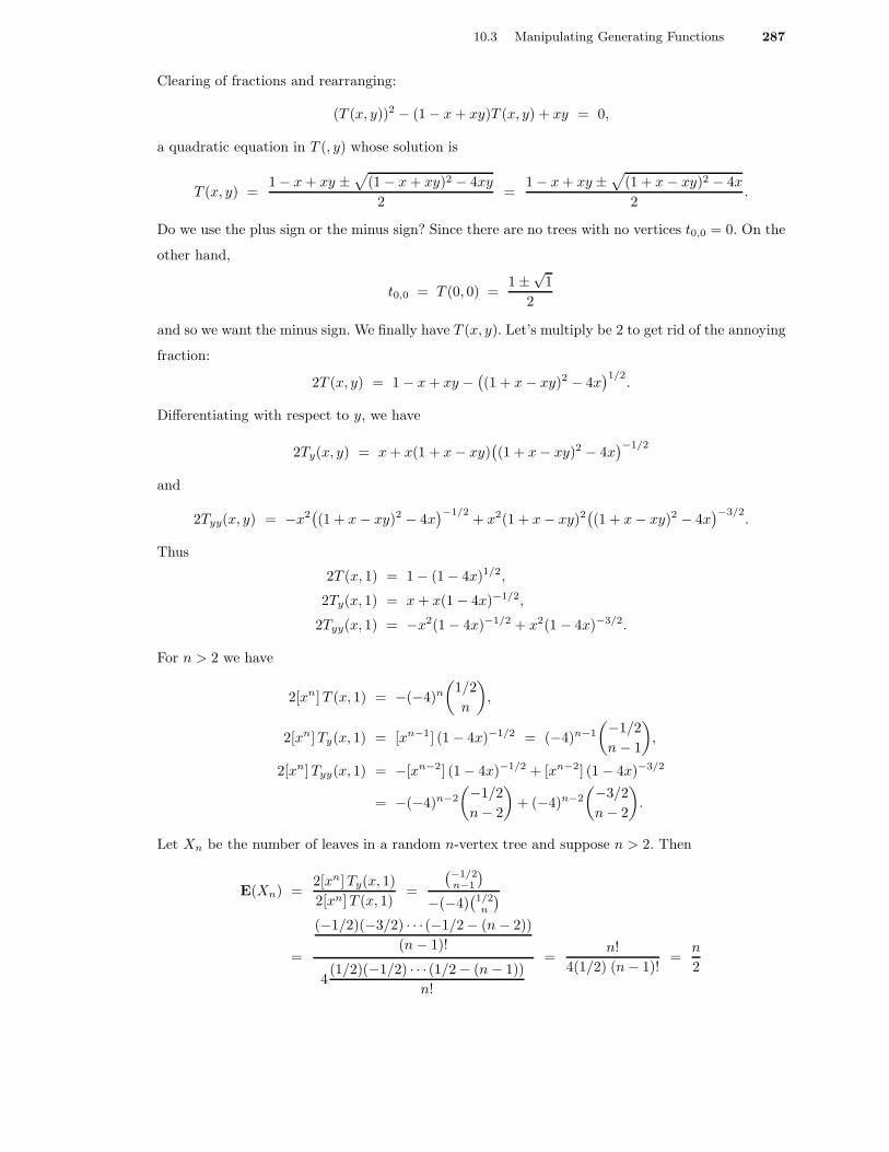
Clearing of fractions and rearranging:
(T (x, y))2 − (1 − x + xy)T (x, y) + xy = 0,
a quadratic equation in T (, y) whose solution is
T (x, y) =1 − x + xy ±
√
(1 − x + xy)2 − 4xy
2=
1 − x + xy ±√
(1 + x − xy)2 − 4x
2.
Do we use the plus sign or the minus sign? Since there are no trees with no vertices t0,0 = 0. On the
other hand,
t0,0 = T (0, 0) =1 ±
√1
2
and so we want the minus sign. We finally have T (x, y). Let’s multiply be 2 to get rid of the annoying
fraction:
2T (x, y) = 1 − x + xy −(
(1 + x − xy)2 − 4x)1/2
.
Differentiating with respect to y, we have
2Ty(x, y) = x + x(1 + x − xy)(
(1 + x − xy)2 − 4x)−1/2
and
2Tyy(x, y) = −x2(
(1 + x − xy)2 − 4x)−1/2
+ x2(1 + x − xy)2(
(1 + x − xy)2 − 4x)−3/2
.
Thus
2T (x, 1) = 1 − (1 − 4x)1/2,
2Ty(x, 1) = x + x(1 − 4x)−1/2,
2Tyy(x, 1) = −x2(1 − 4x)−1/2 + x2(1 − 4x)−3/2.
For n > 2 we have
2[xn] T (x, 1) = −(−4)n
(
1/2
n
)
,
2[xn] Ty(x, 1) = [xn−1] (1 − 4x)−1/2 = (−4)n−1
(−1/2
n − 1
)
,
2[xn] Tyy(x, 1) = −[xn−2] (1 − 4x)−1/2 + [xn−2] (1 − 4x)−3/2
= −(−4)n−2
(−1/2
n − 2
)
+ (−4)n−2
(−3/2
n − 2
)
.
Let Xn be the number of leaves in a random n-vertex tree and suppose n > 2. Then
E(Xn) =2[xn] Ty(x, 1)
2[xn] T (x, 1)=
(−1/2n−1
)
−(−4)(
1/2n
)
=
(−1/2)(−3/2) · · · (−1/2 − (n − 2))
(n − 1)!
4(1/2)(−1/2) · · · (1/2 − (n − 1))
n!
=n!
4(1/2) (n − 1)!=
n
2
288 Chapter 10 Ordinary Generating Functions
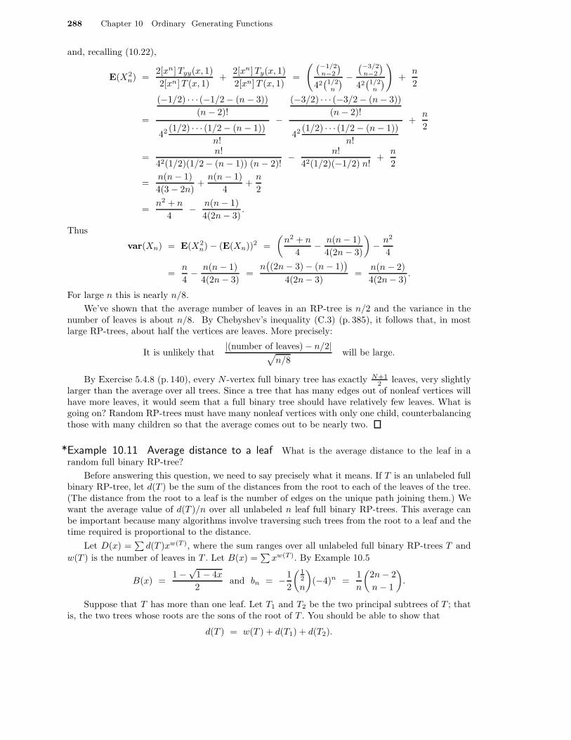
and, recalling (10.22),
E(X2n) =
2[xn] Tyy(x, 1)
2[xn] T (x, 1)+
2[xn] Ty(x, 1)
2[xn] T (x, 1)=
((−1/2
n−2
)
42(
1/2n
)−(−3/2
n−2
)
42(
1/2n
)
)
+n
2
=
(−1/2) · · · (−1/2 − (n − 3))
(n − 2)!
42 (1/2) · · · (1/2 − (n − 1))
n!
−
(−3/2) · · · (−3/2 − (n − 3))
(n − 2)!
42 (1/2) · · · (1/2 − (n − 1))
n!
+n
2
=n!
42(1/2)(1/2− (n − 1)) (n − 2)!− n!
42(1/2)(−1/2) n!+
n
2
=n(n − 1)
4(3 − 2n)+
n(n − 1)
4+
n
2
=n2 + n
4− n(n − 1)
4(2n − 3).
Thus
var(Xn) = E(X2n) − (E(Xn))2 =
(
n2 + n
4− n(n − 1)
4(2n − 3)
)
− n2
4
=n
4− n(n − 1)
4(2n− 3)=
n(
(2n − 3) − (n − 1))
4(2n− 3)=
n(n − 2)
4(2n− 3).
For large n this is nearly n/8.
We’ve shown that the average number of leaves in an RP-tree is n/2 and the variance in thenumber of leaves is about n/8. By Chebyshev’s inequality (C.3) (p. 385), it follows that, in mostlarge RP-trees, about half the vertices are leaves. More precisely:
It is unlikely that|(number of leaves) − n/2|
√
n/8will be large.
By Exercise 5.4.8 (p. 140), every N -vertex full binary tree has exactly N+12 leaves, very slightly
larger than the average over all trees. Since a tree that has many edges out of nonleaf vertices willhave more leaves, it would seem that a full binary tree should have relatively few leaves. What isgoing on? Random RP-trees must have many nonleaf vertices with only one child, counterbalancingthose with many children so that the average comes out to be nearly two.
*Example 10.11 Average distance to a leaf What is the average distance to the leaf in arandom full binary RP-tree?
Before answering this question, we need to say precisely what it means. If T is an unlabeled fullbinary RP-tree, let d(T ) be the sum of the distances from the root to each of the leaves of the tree.(The distance from the root to a leaf is the number of edges on the unique path joining them.) Wewant the average value of d(T )/n over all unlabeled n leaf full binary RP-trees. This average canbe important because many algorithms involve traversing such trees from the root to a leaf and thetime required is proportional to the distance.
Let D(x) =∑
d(T )xw(T ), where the sum ranges over all unlabeled full binary RP-trees T and
w(T ) is the number of leaves in T . Let B(x) =∑
xw(T ). By Example 10.5
B(x) =1 −
√1 − 4x
2and bn = −1
2
(12
n
)
(−4)n =1
n
(
2n − 2
n − 1
)
.
Suppose that T has more than one leaf. Let T1 and T2 be the two principal subtrees of T ; thatis, the two trees whose roots are the sons of the root of T . You should be able to show that
d(T ) = w(T ) + d(T1) + d(T2).

10.3 Manipulating Generating Functions 289
Multiply this by xw(T ) and sum over all T with more than one leaf. Since d(•) = 0 andw(T ) = w(T1) + w(T2), we have
D(x) =∑
n>1
nbnxn +∑
T1,T2
d(T1)xw(T1)+w(T2) +
∑
T1,T2
d(T2)xw(T1)+w(T2)
= xB′(x) − x + D(x)B(x) + B(x)D(x).
Thus
D(x) =xB′(x) − x
1 − 2B(x)=
1√1 − 4x
(
x√1 − 4x
− x
)
=x
1 − 4x− x√
1 − 4x.
It follows that
dn = 4n−1 −( − 1
2
n − 1
)
(−4)n−1 = 4n−1 +n
2
( 12
n − 1
)
(−4)n = 4n−1 − nbn
and so the average distance to a leaf is
4n−1
nbn− 1 =
4n−1
(
2n−2n−1
) − 1.
Using Stirling’s formula, it can be shown that this is asymptotic to√
πn.This number is fairly small compared to n. We could do much better by limiting ourselves to
averaging over certain subclasses of binary RP-trees. For example, we saw in Chapter 8 that if thedistances to the leaves of the tree are all about equal, then the average and largest distances areboth only about log2 n. Thus, when designing algorithms that use trees as data structures, restrict-ing the shape of the tree could lead to significant savings. Good information storage and retrievalalgorithms are designed on this basis.
*Example 10.12 The average time for Quicksort We want to find out how long it takes tosort a list using Quicksort. Quicksort was discussed briefly in Chapter 8. We’ll review it here. Givena list a1, a2, . . . , an, Quicksort selects an element x, divides the list into two parts (greater and lessthan x) and sorts each part by calling itself. There are two problems. First, we haven’t been specificenough in our description. Second, the time Quicksort takes depends on the order of the list andthe way x is chosen at each call. To avoid the dependence on order, we will average over all possi-ble arrangements. We now give a more specific description using x = a1. Given a list a1, a2, . . . , an
of distinct elements, we create a new list s1, s2, . . . , sn with the following properties.
(a) For some 1 ≤ k ≤ n, sk = a1.
(b) si < a1 for i < k and si > a1 for i > k.
(c) The relative order of the elements in the two sublists is the same as in the original list; i.e., ifsi = ap, sj = aq and either i < j < k or k < i < j, then p < q.
It turns out that this can be done with n − 1 comparisons. We now apply Quicksort recursively tos1, . . . , sk−1 and to sk+1, . . . , sn.
Let qn be the average number of comparisons needed to Quicksort an n long list. Thus q1 = 0.We define q0 = 0 for convenience later.
Note that k is the position of a1 in the sorted list. Since the original list is random, all values ofk from 1 to n are equally likely. By analyzing the algorithm carefully, it can be shown that all order-ings of s1, . . . , sk−1 are equally likely as are all orderings of sk+1, . . . , sn. (We will not do this.) Thus,given k, it follows that the average length of time needed to sort both s1, . . . , sk−1 and sk+1, . . . , sn
is qk−1 + qn−k.Averaging over all possible values of k and remembering to include the original n − 1 compar-
isons, we obtain
qn = n − 1 +1
n
n∑
k=1
(
qk−1 + qn−k
)
= n − 1 +2
n
n−1∑
j=0
qj ,
which is valid for n > 0.
290 Chapter 10 Ordinary Generating Functions
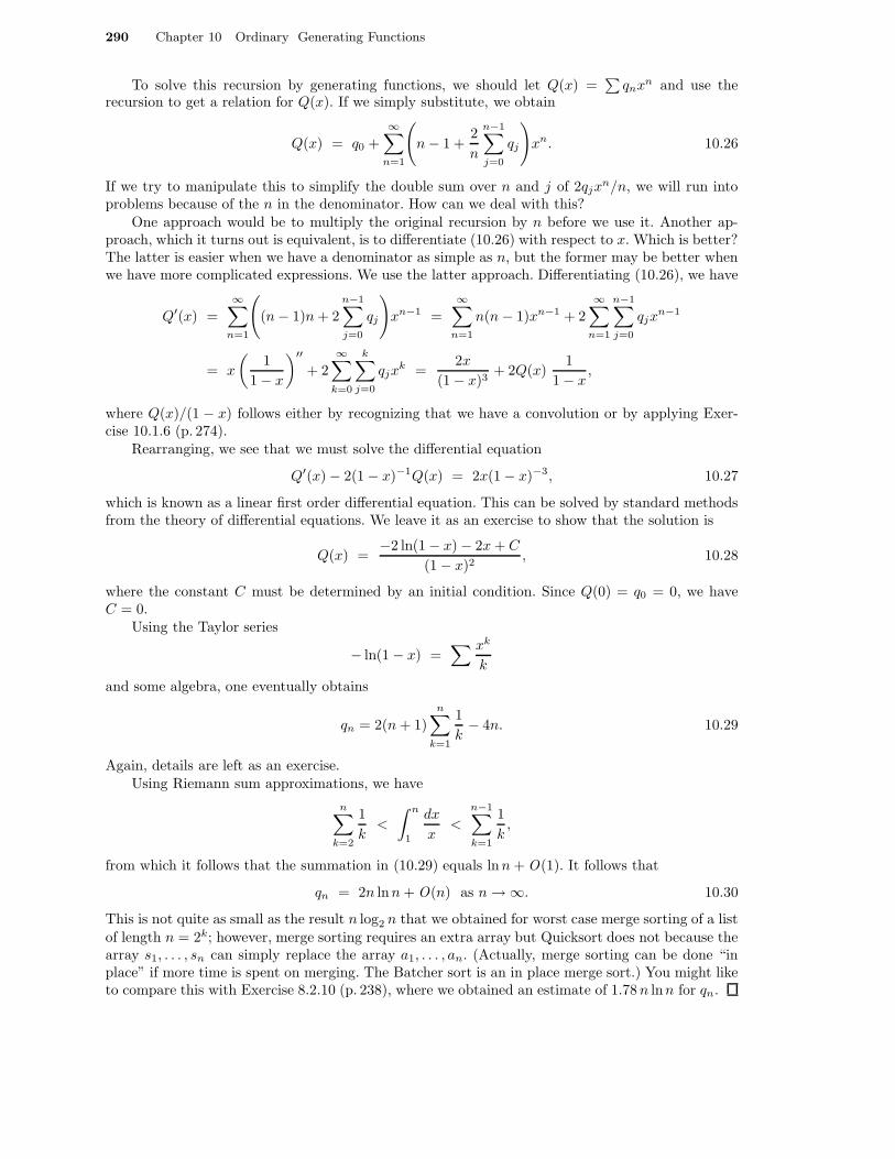
To solve this recursion by generating functions, we should let Q(x) =∑
qnxn and use therecursion to get a relation for Q(x). If we simply substitute, we obtain
Q(x) = q0 +
∞∑
n=1
(
n − 1 +2
n
n−1∑
j=0
qj
)
xn. 10.26
If we try to manipulate this to simplify the double sum over n and j of 2qjxn/n, we will run into
problems because of the n in the denominator. How can we deal with this?One approach would be to multiply the original recursion by n before we use it. Another ap-
proach, which it turns out is equivalent, is to differentiate (10.26) with respect to x. Which is better?The latter is easier when we have a denominator as simple as n, but the former may be better whenwe have more complicated expressions. We use the latter approach. Differentiating (10.26), we have
Q′(x) =
∞∑
n=1
(
(n − 1)n + 2
n−1∑
j=0
qj
)
xn−1 =
∞∑
n=1
n(n − 1)xn−1 + 2
∞∑
n=1
n−1∑
j=0
qjxn−1
= x
(
1
1 − x
)′′+ 2
∞∑
k=0
k∑
j=0
qjxk =
2x
(1 − x)3+ 2Q(x)
1
1 − x,
where Q(x)/(1 − x) follows either by recognizing that we have a convolution or by applying Exer-cise 10.1.6 (p. 274).
Rearranging, we see that we must solve the differential equation
Q′(x) − 2(1 − x)−1Q(x) = 2x(1 − x)−3, 10.27
which is known as a linear first order differential equation. This can be solved by standard methodsfrom the theory of differential equations. We leave it as an exercise to show that the solution is
Q(x) =−2 ln(1 − x) − 2x + C
(1 − x)2, 10.28
where the constant C must be determined by an initial condition. Since Q(0) = q0 = 0, we haveC = 0.
Using the Taylor series
− ln(1 − x) =∑ xk
k
and some algebra, one eventually obtains
qn = 2(n + 1)
n∑
k=1
1
k− 4n. 10.29
Again, details are left as an exercise.Using Riemann sum approximations, we have
n∑
k=2
1
k<
∫ n
1
dx
x<
n−1∑
k=1
1
k,
from which it follows that the summation in (10.29) equals lnn + O(1). It follows that
qn = 2n lnn + O(n) as n → ∞. 10.30
This is not quite as small as the result n log2 n that we obtained for worst case merge sorting of a list
of length n = 2k; however, merge sorting requires an extra array but Quicksort does not because thearray s1, . . . , sn can simply replace the array a1, . . . , an. (Actually, merge sorting can be done “inplace” if more time is spent on merging. The Batcher sort is an in place merge sort.) You might liketo compare this with Exercise 8.2.10 (p. 238), where we obtained an estimate of 1.78 n lnn for qn.
10.4 The Rules of Sum and Product 291
Exercises
10.3.1. Let D(x) be the “exponential” generating function for the number of derangements as in Exam-ple 10.7. You’ll use (10.20) to derive a linear differential equation with polynomial coefficients forD(x). Then you’ll equate coefficients to get a recursion for Dn.
(a) Differentiate (1 − x)D(x) = e−x and the use e−x = (1 − x)D(x) to eliminate e−x.
(b) Equate coefficients to obtain Dn+1 = n(Dn + Dn−1) for n > 0. What are the initial condi-tions?
10.3.2. A “path” of length n is a sequence 0 = u0, u1, . . . , un = 0 of nonnegative integers such thatuk+1 − uk ∈ {−1, 0, 1} for k < n. Let an be the number of such paths of length n The OGF for an
can be shown to be A(x) = (1 − 2x − 3x2)−1/2.
(a) Show that (1 − 2x − 3x2)A′(x) = (1 + 3x)A(x).
(b) Obtain the recursion
(n + 1)an+1 = (2n + 1)an + 3nan−1 for n > 0.
What are the initial conditions?
(c) Use the general binomial theorem to expand (1−(2x+3x2))−1/2 and then the binomial theorem
to expand (2x + 3x2)k. Finally look at the coefficient of xn to obtain an as a sum involvingbinomial coefficients.
10.3.3. Fill in the steps in the derivation of the average time formula for Quicksort:
(a) Solve (10.27) to obtain (10.28) by using an integrating factor or any other method youwish.
(b) Obtain (10.29) from (10.28).
10.3.4. In Exercise 10.2.6, you derived the formula
T (x) =1 − x −
√1 − 2x − 3x2
2x.
Use the methods of this section to derive a recursion for tn that is simpler than the summation inExercise 10.2.6(a).Hint. Since the manipulations involve a fair bit of algebra, it’s a good idea to check your recursionfor tn by comparing it with actual value for small n. They can be determined by constructing thetrees.
10.4 The Rules of Sum and Product
Before the 1960’s, combinatorial constructions and generating function equations were, at best,poorly integrated. A common route to a generating function was:
1. Obtain a combinatorial description of how to construct the structures of interest; e.g., therecursive description of unlabeled full binary RP-trees.
2. Translate the combinatorial description into equations relating elements of the sequence that
enumerate the objects; e.g., bn =∑n−1
k=1 bkbn−k, for n > 1 and b1 = 1.
3. Introduce a generating function for the sequence and substitute the equations into the generatingfunction. Apply algebraic manipulation.
4. The result is a relation for the generating function.
From the 1960’s on, various people have developed methods for going directly from a combinatorialconstruction to a generating function expression, eliminating Steps 2 and 3. These methods often

292 Chapter 10 Ordinary Generating Functions
allow us to proceed from Step 1 directly to Step 4. The Rules of Sum and Product for generatingfunctions are basic tools in this approach. We study them in this section.
So far we have been thinking of generating functions as being associated with a sequence ofnumbers a0, a1, . . . which usually happen to be counting something. It is often helpful to think moredirectly about what is being counted. For example, let B be the set of unlabeled full binary RP-trees.For B ∈ B, let w(B) be the number of leaves of B. Then bn is simply the number of B ∈ B withw(B) = n and so
∑
B∈Bxw(B) =
∑
n
bnxn = B(x). 10.31
We say that B(x) counts unlabeled full binary RP-trees by number of leaves. It is sometimes conve-nient to refer to the generating function by the set that is associated with it. In this case, the set isB so we use the notation GB(x) or simply GB. Thus, instead of asking for the generating functionfor the bn’s, we can just as well ask for the generating function for unlabeled full binary RP-trees(by number of leaves). Similarly, instead of asking for the generating function for Fn, we can ask forthe generating function for sequences of zeroes and ones with no adjacent ones (by the length of thesequence). When it is clear, we may omit the phrase “by number of leaves,” or whatever it is we arecounting things by. We could also keep track of more than one thing simultaneously, like the lengthof a sequence and the number of ones. We won’t pursue that now.
As noted above, if T is some set of structures (e.g., T = B), we let GT be the generating function
for T , with respect to whatever we are counting the structures in T by (e.g., leaves in (10.31)).
The Rule of Sum for generating functions is nothing more than a restatement of the Rule ofSum for counting that we developed in Chapter 1. The Rule of Product is a bit more complex.At this point, you may find it helpful to look back at the Rules of Sum and Product for counting:Theorem 1.2 (p. 6) and Theorem 1.3 (p. 8).
Theorem 10.3 Rule of Sum Suppose a set T of structures can be partitioned into setsT 1, . . . , T j so that each structure in T appears in exactly one T i. It then follows that
GT (x) = GT 1
(x) + · · · + GT j(x).
The Rule of Sum remains valid when the number of blocks in the partition T 1, T 2, . . . is infinite.
Theorem 10.4 Rule of Product Let w be a function that counts something in structures.Suppose each T in a set T of structures is constructed from a sequence T1, . . . , Tk of k structuressuch that
(i) the possible structures Ti for the ith choice may depend on previous choices, but the gen-erating function for them does not depend on previous choices,
(ii) each structure arises in exactly one way in this process and
(iii) if the structure T comes from the sequence T1, . . . , Tk, then
w(T ) = w(T1) + . . . + w(Tk).
It then follows that
GT (x) =∑
T∈Txw(T ) = G1(x) · · ·Gk(x), 10.32
where Gi is the generating function for the possible choices for the ith structure.The Rule of Product remains valid when the number of steps is infinite.

10.4 The Rules of Sum and Product 293
As with the Rule of Product for counting, the available choices for the ith step may depend on the
previous choices, but the generating function must not. If the choices at the ith step do not depend
on the previous choices, we can think of T as simply a Cartesian product T 1 × · · · × T k.
The additivity condition (iii) is needed to insure that multiplication works correctly, namely
xw(T ) = xw(T1) · · ·xw(Tk).
Weights that count things (e.g., leaves in trees, cycles in a permutation, size of set being partitioned)
usually satisfy (iii). This is not always the case; for example, counting the number of distinct things
(e.g., cycle lengths in a permutation) is usually not additive. Weights dealing with a maximum (e.g.,
longest path from root to leaf in a tree, longest cycle in a permutation) do not satisfy (iii).
Proof: We will prove (10.32) by induction on k, starting with k = 2. The induction step is
practically trivial—simply group the first k − 1 choices together as one choice, apply the theorem
for k = 2 to this grouped choice and the kth choice, and then apply the theorem for k − 1 to the
grouped choice.
The proof for k = 2 can be obtained by applying of the Rules of Sum and Product for counting
as follows. Let ti,j be the number of ways to choose the ith structure so that it contains exactly j of
the objects we are counting; that is, the number of ways to choose Ti so that w(Ti) = j. The number
of ways to choose T1 so that it contains j objects AND then choose T2 so that together T1 and T2
contain n objects is t1,j t2,n−j . Thus, the total number of structures in T that contain exactly n
objects isn∑
j=0
t1,j t2,n−j .
Multiplying by xn, summing over n and recognizing that we have a convolution, we obtain (10.32)
for k = 2.
Compare the proof we have just given for k = 2 with the following. By hypotheses (ii) and (iii)
of the theorem,∑
T∈Txw(T ) =
∑
T1∈T 1
xw(T1)
(
∑
T2∈T 2
xw(T2)
)
.
By hypothesis (i), the inner sum equals G2 even though T 2 may depend on T1. Thus the above
expression becomes G1G2. While this might seem almost magical, it’s a perfectly valid proof. The
lesson here is that it’s often easier to sum over structures than to sum over indices.
Passing to the infinite case in the theorems is essentially a matter of taking a limit. We omit
the proof.
Example 10.13 Binomial coefficients Let’s apply these theorems to enumerating binomial
coefficients. Our structures will be subsets of n and we will be keeping track of the number of
elements in a subset; i.e., w(S) = |S|, the number of elements in S. We form all subsets exactly once
by a sequence of n choices. The ith choice will be either ∅ (the empty set) or the set {i}. The union
of our choices will be a subset. The Rule of Product can be applied. Since w(∅) = 0 and w({i}) = 1,
Gi(x) = 1 + x by the Rule of Sum. Thus the generating function for subsets of n by cardinality is
(1 + x) · · · (1 + x) = (1 + x)n. Compare this with the derivation in Example 1.14 (p. 19). Because
this problem is so simple and because you are not familiar with using our two theorems, you may
find the derivation in Example 1.14 easier than the one here. Read on.

294 Chapter 10 Ordinary Generating Functions
Example 10.14 Counting unlabeled RP-trees Let’s look at unlabeled RP-trees from thisnew vantage point. If a tree has more that one vertex, let s1, . . . , sk be the sons of the root from leftto right. We can describe such a tree by listing the k subtrees T1, . . . , Tk whose roots are s1, . . . , sk.This gives us a k-tuple. Note that T has as many leaves as T1, . . . , Tk together. In fact, if you lookback to the start of Chapter 9, you will see that this is nothing more nor less than the definition wegave there.
Let B(x) be the generating function for unlabeled full binary unlabeled RP-trees by numberof leaves. By the previous paragraph, an unlabeled full binary RP-tree is either one vertex OR a2-tuple of unlabeled full binary RP-trees (joined to a new root). Applying the Rules of Sum andProduct with j = k = 2, we have
GB(x) = x + GB(x)GB(x),
which can also be written
B(x) = x + B(x)B(x).
This is much easier than deriving the recursion first—compare this derivation with the one in Ex-ample 10.5 (p. 279).
Now let’s count arbitrary unlabeled RP-trees. In this case, we cannot count them by leavesbecause there are an infinite number of trees with just one leaf: any path is such a tree. We’ll countthem by vertices. Let T (x) be the generating function. Proceeding as in the previous paragraph, wesay that such a tree is either a single vertex, OR one tree, OR a 2-tuple of trees, OR a 3-tuple oftrees, and so on. Thus we (incorrectly) write T (x) = x+ T (x)+ T 2(x)+ · · ·. Why is this wrong? Wedid not apply the Rule of Product correctly. The number of vertices in a tree T is not equal to thetotal number of vertices in the k-tuple (T1, . . . , Tk) that comes from the sons of the root: We forgotthat there is one more vertex, the root of T .
Let’s do this correctly. Instead of a k-tuple of trees, we have a vertex AND a k-tuple of trees.Thus a tree is either a single vertex, OR a single vertex AND a tree, OR a single vertex AND a2-tuple of trees, and so on. Now we get (correctly)
T (x) = x + xT (x) + xT 2(x) + · · · =x
1 − T (x),
by the Rules of Sum and Product and the formula for a sum of a geometric series. Multiplying by1 − T (x), we have T (x) − T 2(x) = x, which is the same as the equation for B(x). Thus
Theorem 10.5 The number of n vertex unlabeled RP-trees equals the number of n leafunlabeled full binary RP-trees.
This was proved in Example 7.9 (p. 206) by showing that the numbers satisfied the same recursionand in Exercise 9.3.12 (p. 266) by giving a bijection.
You should be able to derive T (x) = x + T (x)2 directly from the second definition of RP-treesin Example 7.9 (p. 206) and hence prove the theorem this way.
We’ve looked at two extremes: full binary trees (all nonleaf vertices have exactly 2 children) andarbitrary trees (nonleaf vertices can have any number of children). We can study trees in betweenthese two extremes. Let D be a set of positive integers. Let D be those unlabeled RP-trees wherethe number of children of each vertex lies in D. The two extremes correspond to D = {2} andD = {1, 2, 3, . . .}. If we count these trees by number of vertices, you should be able to show that
GD(x) = x +∑
d∈DxGD(x)d.
In general, we cannot solve this equation; however, we can simplify the sum if the elements of D liein an arithmetic progression. Our two extremes are examples of this. For another example, supposeD is the set of positive odd integers. Then the sum is a geometric series with first term xGD(x) and
ratio GD(x)2. After some algebra, one obtains a cubic equation for GD(x). We won’t pursue this.

10.4 The Rules of Sum and Product 295
Example 10.15 Balls in boxes Problems that involve placing unlabeled balls into labeledboxes (or, equivalently, problems that involve compositions of integers), are often easy to do usingthe Rules of Sum and Product. Let T i be the set of possible ways to put things into the ith box. LetGT i
be the generating function which is keeping track of the things in the ith box. Suppose that
what can be placed into one box is not dependent on what is placed in other boxes. The Rule ofProduct (in the Cartesian product form), tells us that we can simply multiply the GT i
’s together.
How many ways can we put unlabeled balls into k labeled boxes so that no box is empty? Sincethere is exactly one way to place j balls in a box for every j > 0 and no ways if j = 0 (since the boxmay not be empty), we have
GT i(x) = 1x0 + 1x1 + 1x2 + · · · =
∞∑
j=1
xj =x
1 − x
for all i. By the Rule of Product, the generating function is
x
1 − x· · · x
1 − x= xk(1 − x)−k.
Since
xk(1 − x)−k = xk∑
(−k
i
)
(−x)i =∑
(
k + i − 1
i
)
xk+i,
it follows that the number of ways to distribute n unlabeled balls is(
n−1n−k
)
=(
n−1k−1
)
, which you found
in Exercise 1.5.4 (p. 38).
How many solutions are there to the equation z1 + z2 + z3 = n where z1 is an odd positiveinteger and z2 and z3 are nonnegative integers not exceeding 10? We can think of this as placingballs into boxes where zi balls go into the ith box. Since
GT 1
(x) = x + x3 + x5 + · · · = x(
1 + x2 + (x2)2 + (x2)3 + · · ·)
=x
1 − x2
and
GT 2
(x) = GT 3
(x) = 1 + x + · · · + x10 =1 − x11
1 − x,
it follows that the generating function is
x
1 − x2
1 − x11
1 − x
1 − x11
1 − x.
There isn’t a nice formula for the coefficient of xn.
What if we allow positive integer coefficients in our equation? For example, how many solutionsare there to z1 + 2z2 + 3z3 = n in nonnegative integers? In this case, put z1 balls in the first box,2z2 balls in the second and 3z3 balls in the third. Since the number of balls in box i is a multiple ofi, GT i
(x) = 1/(1 − xi). By the Rule of Product GT (x) = 1/((1 − x)(1 − x2)(1 − x3)). This result
can be thought of as counting partitions of the number n where zi is the number of parts of size i.By extending this idea, it follows that, if p(n) is the number of partitions of the integer n, then
∞∑
n=0
p(n)xn =1
1 − x
1
1 − x2
1
1 − x3· · · =
∞∏
i=1
(1 − xi)−1.
So far we have only used the Rules of Sum and Product for single variable generating functions.We need not limit ourselves in this manner. As we will explain:
Observation The Rules of Sum and Product apply to generating functions with any numberof variables.
296 Chapter 10 Ordinary Generating Functions
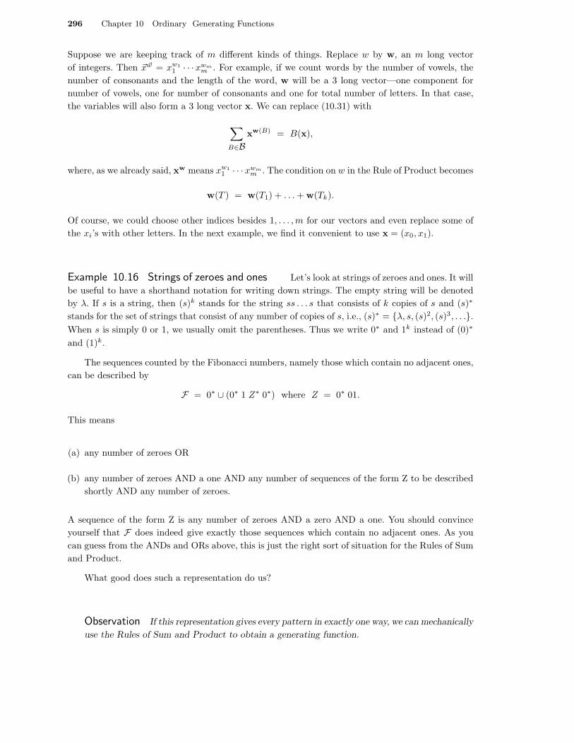
Suppose we are keeping track of m different kinds of things. Replace w by w, an m long vector
of integers. Then ~x~w = xw1
1 · · ·xwmm . For example, if we count words by the number of vowels, the
number of consonants and the length of the word, w will be a 3 long vector—one component for
number of vowels, one for number of consonants and one for total number of letters. In that case,
the variables will also form a 3 long vector x. We can replace (10.31) with
∑
B∈Bxw(B) = B(x),
where, as we already said, xw means xw1
1 · · ·xwmm . The condition on w in the Rule of Product becomes
w(T ) = w(T1) + . . . + w(Tk).
Of course, we could choose other indices besides 1, . . . , m for our vectors and even replace some of
the xi’s with other letters. In the next example, we find it convenient to use x = (x0, x1).
Example 10.16 Strings of zeroes and ones Let’s look at strings of zeroes and ones. It will
be useful to have a shorthand notation for writing down strings. The empty string will be denoted
by λ. If s is a string, then (s)k stands for the string ss . . . s that consists of k copies of s and (s)∗
stands for the set of strings that consist of any number of copies of s, i.e., (s)∗ = {λ, s, (s)2, (s)3, . . .}.When s is simply 0 or 1, we usually omit the parentheses. Thus we write 0∗ and 1k instead of (0)∗
and (1)k.
The sequences counted by the Fibonacci numbers, namely those which contain no adjacent ones,
can be described by
F = 0∗ ∪ (0∗ 1 Z∗ 0∗) where Z = 0∗ 01.
This means
(a) any number of zeroes OR
(b) any number of zeroes AND a one AND any number of sequences of the form Z to be described
shortly AND any number of zeroes.
A sequence of the form Z is any number of zeroes AND a zero AND a one. You should convince
yourself that F does indeed give exactly those sequences which contain no adjacent ones. As you
can guess from the ANDs and ORs above, this is just the right sort of situation for the Rules of Sum
and Product.
What good does such a representation do us?
Observation If this representation gives every pattern in exactly one way, we can mechanically
use the Rules of Sum and Product to obtain a generating function.
10.4 The Rules of Sum and Product 297
For a union (i.e., ∪ or {· · ·}), we are dealing with OR, so the Rule of Sum applies. When symbolsappear to be multiplied it means first one thing AND then another, so we can apply the Rule ofProduct. For a set S, the notation S∗ means any number of copies of things in S. For example,{0, 1}∗ is the set of all strings of zeroes and ones, including the empty string. If there is a unique
way to decompose elements of S∗ into elements in S, then
GS∗ = G∅ + GS + GS×S + GS×S×S + · · · =
∞∑
k=0
(GS )k =1
1 − GS.
What’s “unique” decomposition mean? When S = {0, 1}, every string of zeroes and ones has a uniquedecomposition—just look at each element of the string one at a time. When S = {0, 01, 11} we stillhave unique decomposition; for example, 110001111101 decomposes uniquely as 11-0-01-11-11-01.
We leave it to you to verify that our representation for F gives all the patterns exactly once.Let x0 keep track of zeroes and x1 keep track of ones; that is, the coefficient of xn
0 xm1 in GF (x0, x1)
will be the number sequences in F that have n zeroes and m ones. We have
G0∗ =1
1 − G0=
1
1 − x0= (1 − x0)
−1
GZ∗ = G(0∗ 01)∗ =1
1 − G0∗ 01=
1
1 − (1 − x0)−1x0x1=
1 − x0
1 − x0 − x0x1
GF =1
1 − x0+
1
1 − x0x1
1 − x0
1 − x0 − x0x1
1
1 − x0=
1 + x1
1 − x0 − x0x1.
We can use this representation to describe and count other sequences; however, the problemcan get tricky if we are counting sequences that must avoid patterns more complicated than 11.There are various ways to handle the problem. One method is by the use of sets of recursions, whichwe’ll discuss in the next chapter. Sequences that can be described in this fashion (we haven’t saidprecisely what that means) are called regular sequences. They are, in fact, the strings that can beproduced by regular grammars, which we saw in Section 9.2 were the strings that can be recognizedby finite automata. See Exercise 10.4.19 (p. 304) for a definition and the connection with automata.There is a method for translating finite automata into recursions. We’ll explore this in Example 11.2(p. 310).
We close this section with an example which combines the Rules of Sum and Product with sometechniques for manipulating generating functions.
*Example 10.17 Counting certain spanning trees Let G be a simple graph with V = n∪{0}and the 2n − 1 edges {i, i + 1} (1 ≤ i < n) and {0, j} (1 ≤ j ≤ n). (Draw a picture!) How manyspanning trees does G have? We’ll call the number rn.
To begin with, what does a spanning tree look like? An arbitrary spanning tree can be built asfollows. First, select some of the edges {i, i + 1} (1 ≤ i < n). This gives a graph H with vertex setn. (Some vertices may not be on any edges.) For each component C of H , select a vertex j in C andadd the edge {0, j} to our collection. Convince yourself that this procedure gives all the trees.
We can imagine this in a different way. Let T be the set of rooted trees of the following form.For each k > 0, let V = k ∪ {0} and let 0 be the root. The tree contains the k − 1 edges {i, i + 1}(1 ≤ i < k) and one edge of the form {0, j} for some 1 ≤ j ≤ k. Join together an ordered list of treesin T by merging their roots into one vertex and relabeling their nonroot vertices 1, 2, . . . in order asshown in Figure 10.1. This process produces each spanning tree exactly once.
What we have just described is the perfect setup for the Rules of Sum (on k) and Product (ofT with itself k times) when we count the number of vertices other than the vertex 0. Thus, recallingthe definition of rn at the start of the example,
R =∞∑
k=1
(GT )k =∞∑
k=1
T k =T
1 − T.
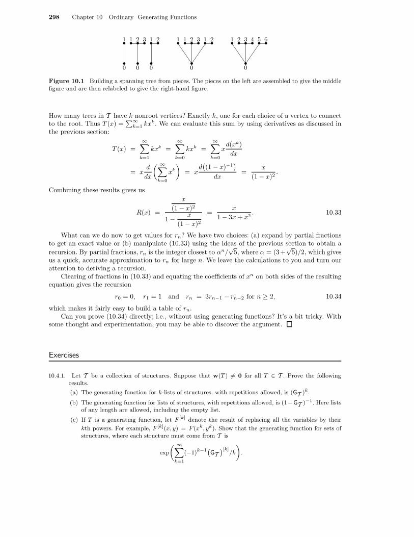
298 Chapter 10 Ordinary Generating Functions
•1
•0
•1 •2
•0
•3 •1
•0
•2
•0
•1 •1 •2 •3 •1 •2
•0
•1 •2 •3 •4 •5 •6
Figure 10.1 Building a spanning tree from pieces. The pieces on the left are assembled to give the middlefigure and are then relabeled to give the right-hand figure.
How many trees in T have k nonroot vertices? Exactly k, one for each choice of a vertex to connectto the root. Thus T (x) =
∑∞k=1 kxk. We can evaluate this sum by using derivatives as discussed in
the previous section:
T (x) =
∞∑
k=1
kxk =
∞∑
k=0
kxk =
∞∑
k=0
xd(xk)
dx
= xd
dx
( ∞∑
k=0
xk
)
= xd(
(1 − x)−1)
dx=
x
(1 − x)2.
Combining these results gives us
R(x) =
x
(1 − x)2
1 − x
(1 − x)2
=x
1 − 3x + x2. 10.33
What can we do now to get values for rn? We have two choices: (a) expand by partial fractionsto get an exact value or (b) manipulate (10.33) using the ideas of the previous section to obtain a
recursion. By partial fractions, rn is the integer closest to αn/√
5, where α = (3+√
5)/2, which givesus a quick, accurate approximation to rn for large n. We leave the calculations to you and turn ourattention to deriving a recursion.
Clearing of fractions in (10.33) and equating the coefficients of xn on both sides of the resultingequation gives the recursion
r0 = 0, r1 = 1 and rn = 3rn−1 − rn−2 for n ≥ 2, 10.34
which makes it fairly easy to build a table of rn.Can you prove (10.34) directly; i.e., without using generating functions? It’s a bit tricky. With
some thought and experimentation, you may be able to discover the argument.
Exercises
10.4.1. Let T be a collection of structures. Suppose that w(T ) 6= 0 for all T ∈ T . Prove the followingresults.
(a) The generating function for k-lists of structures, with repetitions allowed, is (GT )k.
(b) The generating function for lists of structures, with repetitions allowed, is (1−GT )−1. Here listsof any length are allowed, including the empty list.
(c) If T is a generating function, let F [k] denote the result of replacing all the variables by their
kth powers. For example, F [k](x, y) = F (xk, yk). Show that the generating function for sets ofstructures, where each structure must come from T is
exp
( ∞∑
k=1
(−1)k−1(GT)[k]
/k
)
.
10.4 The Rules of Sum and Product 299
Hint. Show that the answer is∏
T∈T(1 + x
w(T )),
replace (1 + xw(T )), with exp(
ln(1 + xw(T )))
, expand the logarithm by Taylor’s Theorem and
rearrange the terms.
(d) Show that generating function for multisets of structures is
exp
( ∞∑
k=1
(
GT)[k]
/k
)
.
10.4.2. Return to Exercise 10.2.4 (p. 280). There we counted the number of sequences of zeros, ones and twoswith no adjacent ones and no adjacent twos. Show that part (a) of that exercise can be rewritten asfollows.A sequence of the type we want is either
• an alternating sequence of ones and twos OR
• a sequence of the type we want AND a zero AND an alternating sequence of ones and twos.
Here the alternating sequence may be empty. Use this characterization to deduce an equation thatcan be solved for S(x)
10.4.3. Using the notation introduced in Example 10.16, write out expressions for strings satisfying thefollowing properties. Do this in such a way that each string is generated uniquely and then use yourrepresentation to get the generating function for the number of patterns of length n. Finally, obtaina recursion from your generating function. Remember to include initial conditions for the recursion.
(a) Strings of zeroes, ones and twos that have do not have the pattern 02 somewhere.Hint. Except possibly for a run of twos at the very start of the string, every 2 must be precededby a 1 or a 2.
(b) Strings of zeroes and ones such that each string of ones is followed by a string of at least k zeroes;i.e., if it starts with a string of zeroes, that can be of any length, but every other string of zeroes
must have length at least k. Use the notation 0k to stand for a string of k zeroes.
(c) Strings of zeroes and ones such that each maximal string of ones (i.e., its ends are the ends ofthe sequence and/or zeroes) has odd length.
10.4.4. Let qn be the number of partitions of n with no repeated parts allowed and, as usual, let pn be allpartitions of n. Let q0 = 1.
(a) Show that
Q(x) =
∞∑
n=0
qnxn =
∞∏
i=1
(1 + xi).
(b) Let P (x) be the generating function for partitions of a number. Show that Q(−x)P (x) = 1.Equate coefficients of xn for n > 0 and then rearrange to avoid subtractions. Interpret therearranged result combinatorially. Can you give a direct proof of it?
(c) Let qn,k (resp. pn,k) be the partitions counted in qn (resp. pn) in which no part exceeds k.
Obtain formulas for∑
n≥0 qn,kxn and∑
n≥0 pn,kxn.

300 Chapter 10 Ordinary Generating Functions
10.4.5. Let a “pile” be, roughly, a two dimensional stack of square blocks resting on a flat surface, with eachblock directly on top of another and each row not having gaps. A more formal definition of a pile ofheight h is a sequence of 2h integers such that
0 = a1 ≤ a2 ≤ · · · ≤ ah < bh ≤ · · · ≤ b2 ≤ b1.
Here a block has width 1 and, counting rows with the first row on the bottom, the left end of row i isat ai and the right end is at bi. The number of blocks in the ith row is bi − ai and the total number
of blocks in the pile is∑h
i=1(bi − ai). Let sn be the number of n-block piles and sn,h the number of
those of height h. Obtain a formula for∑
snxn and∑
n≥0 sn,hxn.
Hint. The generating function for partitions with no part exceeding k will be useful.
10.4.6. Let a1 < a2 < · · · < ak be a k element subset of n = {1, 2, . . . , n}. We will study subsets withrestrictions on the ai.
(a) Let a0 = 0. By looking at ai − ai−1, show that there is a bijection between k element subsets ofn and k long sequences of positive integers with sum not exceeding n.
(b) Let un be the number of k element subsets of n. Use (a) to show that
U(x) =(
∑
i≥1
xi)k (∑
i≥0
xi)
=xk
(1 − x)k+1.
(Do not use the fact that(−k−1
n−k
)
=(
nn−k
)
.)
(c) Let tn be the number of k element subsets a1 < a2 < · · · of n such that i and ai have the sameparity. In other words a2j is even and a2j+1 is odd. Show that
T (x) =xk
(1 − x2)k1
1 − x=
(1 + x)xk
(1 − x2)k+1.
(d) Let bxc be the result of rounding x down; e.g., b3.5c = 3. Show that tn =(b(n+k)/2c
k
)
.
(e) We call (ai, ai+1) a succession if they differ by one. Let sn,j be the number of k element subsetsof n with exactly j successions. Show that
S(x, y) =1
1 − x
x
1 − x(xy + x2 + x3 + · · ·)k−1 =
xk(x + y(1 − x))k−1
(1 − x)k+1.
(f) Show that∑
n≥0 sn,jxn =
(
k−1j
)
x2k−j−1(1 − x)−(k+1−j).
(g) Express sn,j as a product of two binomial coefficients. Check your result by listing all 4 element
subsets of {1, . . . , 6} and determining how many successions they have.
10.4.7. Recall that a binary RP-tree to be an RP-tree where each vertex may have at most two sons. Theset T of such trees was studied in Exercise 10.2.6, where we counted them by number of vertices.
(a) Using the Rules of Sum and Product, derive the relation T (x) = x + xT (x) + xT (x)2 that ledto
T (x) =1 − x −
√1 − 2x − 3x2
2x
in Exercise 10.2.6
(b) Discuss how you might compute the number of such trees. In particular, can you find a simpleexpression as a function of n?
10.4.8. Change the definition in Exercise 10.4.7 so that, if a node has just one son, then we distinguishwhether or not it is a right or a left son. (This somewhat strange sounding distinction is sometimesimportant.) How many such trees are there with n internal vertices?
10.4 The Rules of Sum and Product 301
10.4.9. A rooted tree will be called “contractible” if it has a vertex with just one son since one can imaginecombining that vertex’s information with the information at its son.
(a) Find the generating function for the number of unlabeled noncontractible RP-trees, countingthem by number of vertices.
(b) Find the generating function for the number of unlabeled noncontractible RP-trees, countingthem by number of leaves.
(c) Obtain a linear differential equation with polynomial coefficients and thence a recursion fromeach of the generating functions in this problem.Hint. Solve for the square root, differentiate, multiply by the square of the square root and thenreplace the square root that remains.
10.4.10. Let tn,k be the number of RP-trees with n leaves and k internal vertices (i.e., nonleaves).
(a) Find a generating function for T (x, y).
(b) Using the previous result, prove that tn,k = tk,n when n + k > 1.
Hint. Compare T (x, y) and T (y, x).
*(c) Find a bijection that proves tn,k = tk,n when n + k > 1; that is, find a map from RP-trees
to RP-trees that carries leaves to internal vertices and vice versa for trees with more than onevertex. Write out your bijection for RP-trees with 5 vertices.Hint. Describe the construction recursively (or locally).
10.4.11. Let D be a set of nonnegative integers such that 0 ∈ D. For this exercise, we’ll say that an RP-treeis of outdegree D if the number of sons of each vertex lies in D. Thus, full binary RP-trees are ofoutdegree {0, 2}.
(a) Let TD(x) be the generating function for unlabeled RP-trees of outdegree D by number ofvertices. Prove that
TD(x) = x∑
d∈D
TD(x)d
(b) Show that the previous formula allows us to compute TD(x) recursively.
(c) Let LD(x) be the generating function for unlabeled RP-trees of outdegree D by number of leaves.Show that it doesn’t make sense to talk about LD(x) when 1 ∈ D, that
LD(x) =∑
d∈D
LD(x)d − 1 + x,
and that this allows us to compute LD(x) recursively when 1 /∈ D.
10.4.12. We have boxes labeled with pairs of numbers like (2, 6). The labels have the form (i, j) for 1 ≤ i ≤ 3and 1 ≤ j ≤ k. Thus we have 3k boxes. Unlabeled balls are placed into the boxes. This must be doneso that the number of balls in box (i, j) is a multiple of i and, for each j, the total number of ballsin boxes (1, j), (2, j) and (3, j) is at most 5. What is the generating function for the number of waysto place n balls?Hint. Find the generating function for placing balls into (1, ∗), (2, ∗) and (3, ∗) and then use the Ruleof Product.
*10.4.13. An unlabeled full binary rooted tree is like the ordered (i.e., plane) situation except that we makeno distinction between left and right sons. Let βn be the number of such trees with n leaves and let
B(x) =∑
βnxn. Show that B(x) = x + (B(x)2 + B(x2))/2.
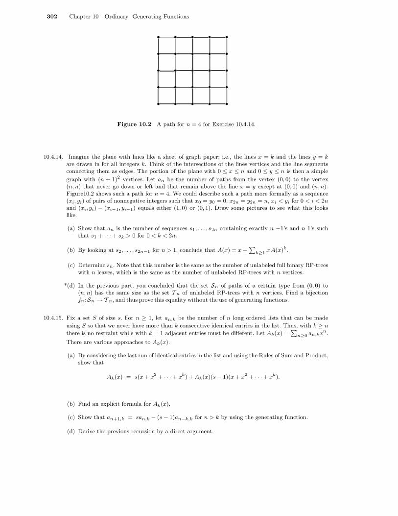
302 Chapter 10 Ordinary Generating Functions
• • • • •
• • • • •
• • • • •
• • • • •
• • • • •
Figure 10.2 A path for n = 4 for Exercise 10.4.14.
10.4.14. Imagine the plane with lines like a sheet of graph paper; i.e., the lines x = k and the lines y = kare drawn in for all integers k. Think of the intersections of the lines vertices and the line segmentsconnecting them as edges. The portion of the plane with 0 ≤ x ≤ n and 0 ≤ y ≤ n is then a simple
graph with (n + 1)2 vertices. Let an be the number of paths from the vertex (0, 0) to the vertex(n, n) that never go down or left and that remain above the line x = y except at (0, 0) and (n, n).Figure10.2 shows such a path for n = 4. We could describe such a path more formally as a sequence(xi, yi) of pairs of nonnegative integers such that x0 = y0 = 0, x2n = y2n = n, xi < yi for 0 < i < 2nand (xi, yi) − (xi−1, yi−1) equals either (1, 0) or (0, 1). Draw some pictures to see what this lookslike.
(a) Show that an is the number of sequences s1, . . . , s2n containing exactly n −1’s and n 1’s suchthat s1 + · · · + sk > 0 for 0 < k < 2n.
(b) By looking at s2, . . . , s2n−1 for n > 1, conclude that A(x) = x +∑
k≥1 x A(x)k.
(c) Determine sn. Note that this number is the same as the number of unlabeled full binary RP-treeswith n leaves, which is the same as the number of unlabeled RP-trees with n vertices.
*(d) In the previous part, you concluded that the set Sn of paths of a certain type from (0, 0) to(n, n) has the same size as the set T n of unlabeled RP-trees with n vertices. Find a bijectionfn:Sn → T n, and thus prove this equality without the use of generating functions.
10.4.15. Fix a set S of size s. For n ≥ 1, let an,k be the number of n long ordered lists that can be made
using S so that we never have more than k consecutive identical entries in the list. Thus, with k ≥ n
there is no restraint while with k = 1 adjacent entries must be different. Let Ak(x) =∑
n≥0 an,kxn.
There are various approaches to Ak(x).
(a) By considering the last run of identical entries in the list and using the Rules of Sum and Product,show that
Ak(x) = s(x + x2 + · · · + xk) + Ak(x)(s − 1)(x + x2 + · · · + xk).
(b) Find an explicit formula for Ak(x).
(c) Show that an+1,k = san,k − (s − 1)an−k,k for n > k by using the generating function.
(d) Derive the previous recursion by a direct argument.
10.4 The Rules of Sum and Product 303
10.4.16. We claim that the set of sequences of zeroes and ones that do not contain either 101 or 111 isdescribed by
0∗ ∪(
0∗(1 ∪ 11)(
000∗(1 ∪ 11))∗
0∗)
and each such sequence has a unique description. You need not verify this. Let an be the number ofsuch sequences of length n and let A(x) be the generating function for an.
(a) Derive the formula A(x) = 1+x+2x2+x3
1−x−x3−x4 .
(b) Using A(x), obtain the recursion an = an−1 + an−3 + an−4 for n ≥ 4 and find the initialconditions.
(c) Using 1 − x − x3 − x4 = (1 − x − x2)(1 + x2), derive the formula
an =7Fn+1 + 4Fn − bn
5where bn =
{
2(−1)n/2, if n is even,
(−1)(n−1)/2, if n is odd,
where the Fibonacci numbers are given by F0 = 0, F1 = 1 and Fn = Fn−1 + Fn−2 for n ≥ 2;that is, their generating function is x
1−x−x2 .
(d) Prove that
a2n = F 2n+2 and a2n+1 = Fn+2Fn+3 for n ≥ 0.
Hint. Show that the recursion and initial conditions are satisfied.
10.4.17. Using partial fractions, obtain a formula for rn from (10.33).
*10.4.18. Let G be the simple graph with vertex set n∪{0} and the 2n edges {n, 1}, {i, i + 1} (1 ≤ i < n) and{0, j} (1 ≤ j ≤ n), except for n = 1, 2 where we must avoid adding {n, 1} in order to get a simplegraph. In other words, G is like the graph in Example 10.17 except that one more edge {1, n} hasbeen added so that the picture looks like a wheel with spokes for n > 2. We want to know how manyspanning trees G has.
(a) Let T be as in Example 10.17 and let T ′ consist of the trees in T with one of the nonroot vertices
marked. Choose one tree from T ′ and then a, possibly empty, sequence of trees from T . Supposewe have a total of n nonroot vertices. Merge the root vertices and relabel the nonroot vertices 1 to
n, starting with the marked vertex in the tree from T ′ and preceding cyclically until all nonrootvertices have been labeled. Explain why this gives all the spanning trees exactly once.
(b) Show that GT ′(x) = x(d/dx)(GT (x)) = x(1 + x)/(1 − x)3.
(c) Show that generating function for the spanning trees is
x(1 + x)
(1 − x)(1 − 3x + x2).
(d) Show that the number of spanning trees is 2rn+1−3rn−2, where rn is given in Example 10.17.
304 Chapter 10 Ordinary Generating Functions
10.4.19. We define a set of regular sequences (or regular strings) on the “alphabet” A. (An alphabet is anyfinite set.) Let R, R1, and R2 stand for sets of regular strings on A. The sets of regular strings onA are the empty set, the sets {a} where a ∈ A, and the sets that can be built recursively using thefollowing operations:
• union (“or”) of sets, i.e., the set of all strings that belong to either R1 or R2;
• juxtaposition (“and then”), i.e., the set of all strings r1r2 where r1 ∈ R1 and r2 ∈ R2;
• arbitrary iteration R∗, i.e., for all n ≥ 0, all strings of the form r1r2 . . . rn where ri ∈ R.(The empty string is obtained when n = 0.)
See Example 10.16 for a specific example of a set of regular sequences The purpose of this exerciseis to construct a nondeterministic finite automaton that recognizes any given set of regular strings.Nondeterministic finite automata are defined in Section 6.6 (p. 189). We will build up the machineby following the way the strings are built up.
(a) Let A be an automaton. Show that there is another automaton S(A) that recognizes the samestrings and has no edges leading into the start state.Hint. Create a new state, let it be the start state and let it have edges to all of the states theold start state did. Remember to specify the accepting states, too.
(b) If A recognizes the set A and B recognizes the set B, construct and automaton that recognizesthe set A ∪ B.Hint. Adjust the idea in (a).
(c) If A recognizes A, construct an automaton that recognizes A∗.Hint. Add some edges.
(d) If A recognizes the set A and B recognizes the set B, construct and automaton that recognizesAB; i.e., the set A × B.
Notes and References
The classic books on generating functions are those by MacMahon [6] and Riordan [7]. They arequite difficult reading and do not take a “combinatorial” approach to generating functions. There arevarious combinatorial approaches. Some can be found in the texts by Wilf [10] and Stanley [9, Ch. 3]and in the articles by Bender and Goldman [1] and Joyal [5]. The articles are rather technical.
Parts of the texts by Greene and Knuth [4] and by Graham, Knuth and Patashnik [3] are orientedtoward computer science uses of generating functions. See also the somewhat more advanced textby Sedgewick and Flajolet [7]. Wilf [10] gives a nice introduction to generating functions. Gouldenand Jackson’s book [2] contains a wealth of material on generating functions, but is at a higher levelthan our text.
We have studied only the simplest sorts of recursions. Recursions that require more sophisti-cated methods are common as are recursions that cannot be solved exactly. Sometimes approximatesolutions are possible. We don’t know of any systematic exposition of techniques for such problems.
We have not dealt with the problem of defining formal power series; that is, defining a generatingfunction so that the convergence of the infinite series is irrelevant. An introduction to this can befound in the first few pages of Stanley’s text [9].
1. Edward A. Bender and Jay R. Goldman, Enumerative uses of generating functions, Indiana
Univ. Math. J. 20 (1971), 753–765.
2. Ian P. Goulden and David M. Jackson, Combinatorial Enumeration, Dover (2004).
3. Ronald L. Graham, Donald E. Knuth and Oren Patashnik, Concrete Mathematics, 2nd ed.,Addison-Wesley, Reading (1994).
4. Daniel H. Greene and Donald E. Knuth, Mathematics for the Analysis of Algorithms, 3rd ed.,Birkhauser (1990).

Notes and References 305
5. Andre Joyal, Une theorie combinatoire des series formelles, Advances in Math. 42 (1981), 1-82.
6. Percy Alexander MacMahon, Combinatory Analysis, Chelsea, New York, 1960. Reprint of twovolume Cambridge Univ. Press edition (1915, 1916).
7. John Riordan, An Introduction to Combinatorial Analysis, Princeton Univ. Press (1980).
8. Robert Sedgewick and Philippe Flajolet, An Introduction to the Analysis of Algorithms, Addison-Wesley (1996).
9. Richard P. Stanley, Enumerative Combinatorics, vols. 1 and 2. Cambridge Univ. Press (1999,2001).
10. Herbert S. Wilf, Generatingfunctionology, 2nd ed., Academic Press (1993).