order picking optimization in a distribution center
TRANSCRIPT

ORDER PICKING OPTIMIZATION IN A DISTRIBUTION CENTER
Master’s Thesis Jussi Engblom Aalto University School of Business Information and Service Management Spring 2020
Aalto University, P.O. BOX 11000, 00076 AALTO www.aalto.fi
Abstract of master’s thesis Author Jussi Engblom Title of thesis ORDER PICKING OPTIMIZATION IN A DISTRIBUTION CENTER Degree Master of Science (Economics and Business Administration) Degree programme Information and Service Management Thesis advisor(s) Tomi Seppälä, Otto Sormunen, Ville Mattila Year of approval 2020 Number of pages 62 Language English
Abstract This study focuses on the order picking process of a distribution center (DC) supplying locomotive and railroad car parts. The DC employs a manual picker-to-parts system where pickers move on foot or by vehicular means. Efficiency of an order picking process in such a DC mainly depends on three problems when the layout of the DC is given: the storage location assignment problem (SLAP), the order batching problem and the order picker routing problem. This study focuses on the aggregate effect three major decisions have on order picking performance in a manual picker-to-parts ware-house. To study the effects of these three sub-problems, we create a framework that allows us to run sim-ulated scenarios with different approaches to these problems. To solve the SLAP, we employ a hybrid of class-based and family grouping methods by enhancing a class-based SKU location assignment with modern clustering techniques. To further improve the order picking process, we experiment with various order batching methods. We use picker routing heuristics to evaluate combinations of the storage location assignments and batching procedures. Over a set of order lines to be fulfilled, the objective function is be the aggregate distance covered over the warehouse floor. We show that distance savings of more than 55% can be achieved by rearranging the DC. Moreover, we show that stock keeping unit (SKU) clustering can improve the performance of class-based storage location assignments and that even simple order batching algorithms are likely to improve order picking performance significantly. Based on the framework, we develop a tool set that encompasses the aspects concerning the DC’s order picking process. The solution will be implemented into a cloud-computing environment, al-lowing for real-time tracking of the DC’s order picking efficiency and the generation of visual tools that help move SKUs to desirable shelf locations and batch orders. Keywords order picking, heuristics, clustering, picker routing, distribution center

Aalto-yliopisto, PL 11000, 00076 AALTO www.aalto.fi
Maisterintutkinnon tutkielman tiivistelmä Tekijä Jussi Engblom Työn nimi JAKELUKESKUKSEN KERÄILYTOIMINNAN OPTIMOINTI Tutkinto Kauppatieteiden maisteri Koulutusohjelma Tieto- ja palvelujohtaminen Työn ohjaaja(t) Tomi Seppälä, Otto Sormunen, Ville Mattila Hyväksymisvuosi 2020 Sivumäärä 62 Kieli englanti
Tiivistelmä Tutkimus keskittyy veturien ja junavaunujen osia varastoivan jakelukeskuksen keräilyprosessiin. Jakelukeskuksen keräily suoritetaan jalan tai erilaisilla kulkuneuvoilla. Kolme suurinta keräilytoiminnan tehokkuuteen vaikuttavaa tekijää ovat varastoitavien nimikkeiden sijoittelu, tilausten yhdistely suuremmiksi kokonaisuuksiksi sekä keräilijän reitittäminen. Tässä tutkimuksessa tutkitaan näiden tekijöiden vaikutusta keräilyn tehokkuuteen. Loimme viitekehyksen, jonka avulla voidaan arvioida näiden kolmen aliongelman vaikutusta keräilyn tehokkuuteen simulaatiomallien avulla. Nimikkeiden sijoitteluongelma ratkaistiin luokka- ja klusteriperusteisten strategioiden hybrideillä. Tilausten yhdistelyongelma taas ratkaistiin kahdella heuristiikalla. Erilaisten nimikesijoitteluiden ja tilausyhdistelystrategioiden kombinaatioiden tehokkuuden mittaaminen suoritettiin jakelukeskusta varten luodulla keräilijän reititysheuristiikalla. Päätösmuuttujana käytettiin tietyn tilausjoukon sisältämien keräilyrivien keräämiseen käytettyä matkaa. Parhailla kombinaatioilla saavutettiin yli 55 prosentin säästö nykytilanteeseen verrattuna. Lisäksi todettiin, että luokkaperusteista nimikesijoittelua on mahdollista tehostaa klusteroimalla nimikkeitä. Tulokset osoittavat myös, että tilausten yhdisteleminen on erittäin kannattavaa ja yksinkertaisillakin menetelmillä saavutetaan suuret hyödyt. Viitekehyksen pohjalta rakennettiin työkalu, jonka avulla voidaan hallita ja havainnoida jakelukeskuksen keräilyprosessia. Työkalu implementoitiin pilvipalveluratkaisuna osaksi tilaajayrityksen varastonhallintaprosessia. Sen avulla voidaan seurata visuaalisten esitysten avulla keräilyn tehokkuuden kehitystä, suunnitella muutoksia nimikesijoitteluun ja yhdistellä tilauksia. Avainsanat keräily, heuristiikka, klusterointi, reititys, jakelukeskus
i
ContentsContents i
1 Introduction 1
2 Literature review 42.1 Warehouse layout . . . . . . . . . . . . . . . . . . . . . . . . . . . . . . 52.2 Storage location assignment strategies . . . . . . . . . . . . . . . . . . . 5
2.2.1 Class-based assignments . . . . . . . . . . . . . . . . . . . . . . 62.2.2 Correlation-based assignments . . . . . . . . . . . . . . . . . . . 8
2.3 Order batching methods . . . . . . . . . . . . . . . . . . . . . . . . . . . 92.4 Picker routing methods . . . . . . . . . . . . . . . . . . . . . . . . . . . 10
3 Research material and methods 143.1 Data . . . . . . . . . . . . . . . . . . . . . . . . . . . . . . . . . . . . . 14
3.1.1 The layout . . . . . . . . . . . . . . . . . . . . . . . . . . . . . 153.1.2 The stock level report . . . . . . . . . . . . . . . . . . . . . . . . 173.1.3 Historical SKU demand and order pick lists . . . . . . . . . . . . 18
3.2 Class-based storage assignments . . . . . . . . . . . . . . . . . . . . . . 193.2.1 Class generation . . . . . . . . . . . . . . . . . . . . . . . . . . 203.2.2 Zone divisions . . . . . . . . . . . . . . . . . . . . . . . . . . . 21
3.3 Correlation-based storage assignments . . . . . . . . . . . . . . . . . . . 233.3.1 OPTICS . . . . . . . . . . . . . . . . . . . . . . . . . . . . . . . 273.3.2 Sum-seed algorithm . . . . . . . . . . . . . . . . . . . . . . . . 28
3.4 Order batching . . . . . . . . . . . . . . . . . . . . . . . . . . . . . . . 293.4.1 Seed batching . . . . . . . . . . . . . . . . . . . . . . . . . . . . 313.4.2 Random batching . . . . . . . . . . . . . . . . . . . . . . . . . . 32
3.5 Picker routing with modified s-shape heuristic . . . . . . . . . . . . . . . 333.6 Framework . . . . . . . . . . . . . . . . . . . . . . . . . . . . . . . . . 35
4 Results 384.1 Dataset description and performance measures . . . . . . . . . . . . . . . 384.2 Effects of the storage location assignments . . . . . . . . . . . . . . . . . 394.3 Effects of the order batching heuristics . . . . . . . . . . . . . . . . . . . 434.4 Accuracy and reliability of the method . . . . . . . . . . . . . . . . . . . 46
5 Discussion, practical implications and conclusions 495.1 Discussion . . . . . . . . . . . . . . . . . . . . . . . . . . . . . . . . . . 495.2 Practical implications . . . . . . . . . . . . . . . . . . . . . . . . . . . . 515.3 Conclusions . . . . . . . . . . . . . . . . . . . . . . . . . . . . . . . . . 53
References 55
A Normalized pairwise frequencies for the fastest SKUs 58
B OPTICS reachability plot 59

ii
C Performance of storage location assignments and batching combinations. 60
D Visualization tool 62

iii
List of Tables1 Stock place distribution by block. . . . . . . . . . . . . . . . . . . . . . 162 Stock place distributions for zone variants 1, 2 and 3. . . . . . . . . . . . 223 Pick lists by type. . . . . . . . . . . . . . . . . . . . . . . . . . . . . . . 384 ABC-1 Monte Carlo experiment. . . . . . . . . . . . . . . . . . . . . . . 48A1 Normalized pairwise frequencies for the fastest SKUs. . . . . . . . . . . 58C1 Performance of alternative storage location assignments. . . . . . . . . . 60C2 Performance of all batching and storage location assignment combinations. 61
iv
List of Figures1 The across-aisle (top), within-aisle (middle) and diagonal (bottom) policies. 82 Common routing heuristics in a three-block warehouse as illustrated by
Roodbergen and De Koster (2001a). . . . . . . . . . . . . . . . . . . . . 113 Layout of the distribution center. . . . . . . . . . . . . . . . . . . . . . . 154 Pallet item demand distribution . . . . . . . . . . . . . . . . . . . . . . 215 ABC-1 zone divisions. . . . . . . . . . . . . . . . . . . . . . . . . . . . 226 ABC-2 zone divisions. . . . . . . . . . . . . . . . . . . . . . . . . . . . 237 ABC-3 zone divisions. . . . . . . . . . . . . . . . . . . . . . . . . . . . 238 The ABC-1 assignment with the cluster assignment. . . . . . . . . . . . . 269 Relationship of pallet item lines and small item lines. . . . . . . . . . . . 3010 The 16 common pick locations in the first four blocks of the DC. . . . . . 3211 The five common pick locations in the last two blocks of the DC. . . . . . 3212 Picker routes in the four first blocks of the DC. The depot is marked with a
black circle. . . . . . . . . . . . . . . . . . . . . . . . . . . . . . . . . . 3413 Picker routes in the two rear blocks of the DC. . . . . . . . . . . . . . . 3414 Example route generated by the s-shape algorithm. . . . . . . . . . . . . 3515 The order picking framework. . . . . . . . . . . . . . . . . . . . . . . . 3616 Absolute performance of all storage location assignments. . . . . . . . . 3917 Relative performance of all storage location assignments. . . . . . . . . 4018 Moving average time series for selected assignments. . . . . . . . . . . . 4119 ABC-3 route length distribution. . . . . . . . . . . . . . . . . . . . . . . 4220 C-ABC-3 route length distribution. . . . . . . . . . . . . . . . . . . . . . 4221 Relative performance of the seed and the random batching algorithms
compared to FCFS. . . . . . . . . . . . . . . . . . . . . . . . . . . . . . 4322 Relative performance of all batching and storage location assignment
combinations. . . . . . . . . . . . . . . . . . . . . . . . . . . . . . . . . 4423 Absolute performance of all batching and storage location assignment
combinations. . . . . . . . . . . . . . . . . . . . . . . . . . . . . . . . . 45B1 The reachability plot generated by the OPTICS algorithm. . . . . . . . . 59D1 Visualization tool example. . . . . . . . . . . . . . . . . . . . . . . . . . 62

Introduction 1
1 Introduction
The order picking process is often neglected, although it is the major cost component in
any warehouse and strongly affects supply chain performance. Of all the operations in
a warehouse, order picking is usually the most cost-intensive. In a manually operated
warehouse, order picking involves personnel moving around the warehouse collecting
orders. We define an order as a list of items that the order picker collects during a single
tour around the warehouse. Traveling around the warehouse is laborious and it often
requires a lot of time compared to other warehouse activities. Time spent traveling around
the warehouse collecting items is a non-value-adding direct cost (Bartholdi and Hackman
2011). Therefore, the time spent picking orders should be minimized.
Over the years, the demand structure of many warehouses has changed such that order
sizes have become smaller and orders need to be fulfilled faster (Le-Duc and De Koster
2005). This gives warehouse managers incentive to enhance the efficiency of their order
picking operations. Moreover, literature shows that the implementation of different order
batching methods, picker routing methods and storage location assignment strategies can
drastically reduce the costs attributable to the order picking process (Caron, Marchet, and
Perego 1998). De Koster, Le-Duc, and Roodbergen (2007) argue that in Western Europe,
over 80% of all warehouses are manual picker-to-parts systems, meaning that the issue of
order picking efficiency remains prevalent.
This study concentrates on the optimization of the order picking process in a large dis-
tribution center. The sub-problems faced in this thesis are the storage location assignment
problem (SLAP), the picker routing problem and the order batching problem, which are
the three the main factors affecting order picking efficiency when the warehouse layout
is fixed. For the case distribution center, which specializes in locomotive and railroad
car parts, the efficiency of the order picking process is a primary concern. In addition to
supplying other warehouses of the case firm, the distribution center must deliver orders to
nearby production units throughout the day. Orders from the production units must often
be fulfilled instantly. This requires an order picking process that can output stock-keeping
units (SKU) as quickly as possible. Stock-keeping units can be thought as the different
products or items that reside in a warehouse. SKUs may be be classified based on various
criteria; the case distribution center stores an especially wide range of SKUs ranging from
minuscule items to items weighing tons.
Minimizing the time required to pick orders is analogous to minimizing the distance
traveled in the distribution center. This is a complex optimization problem comprising
many moving parts. The optimization problem concerning the efficiency of the order

Introduction 2
picking process can be divided into four major intertwining decisions. They are 1) the
warehouse layout problem, 2) the storage location assignment problem (SLAP), 3) the order
batching problem and 4) the picker routing problem. Literature has shown multiple ways to
approach each one of these problems. For instance, order batching literature knows dozens
of algorithms that try to solve the batching problem from different angles. Moreover, both
the order batching problem and the picker routing problem are NP-hard, with the routing
problem being a special case of the traveling salesman problem. Most of the time, trying
to find global optima to these problems is useless: the demand characteristics of SKUs are
not constant, but stochastic, and change over time. The sub-problems of the order picking
process are challenging and vast on their own, but only when they are considered in unison,
the complexity of the order picking process really emerges.
The four decisions each deal with a different issue, although they are all relate to each
other and must therefore be considered in unison. The layout problem deals with the
physical dimensions of the warehouse: the number of racks and blocks, aisle configuration,
rack height to name a few. The storage location assignment problem concerns the placement
of the SKUs on the racks of the warehouse. This problem relates closely to the layout
problem in the design phase of the warehouse. Order batching is a method to improve
the efficiency of a warehouse by joining multiple orders into a single order pick list such
that the the number of tours that must be completed is reduced. The batching problem is
closely related to location assignment problem: SKU locations are used to determine the
best batches. The picker routing strategy of a warehouse defines the order in which the
order picker travels the aisles of the warehouse. Routing strategies are used to minimize
the distance the order picker must travel to collect orders.
The goal of this study is to find ways to improve the performance of the order picking
process in the case distribution center. An important criterion is that the solutions proposed
by the model have monetary value and that their implementation is feasible. Hence,
the research question is: "what is the most robust and optimal way to arrange the order
picking process of the manually operated case distribution center to minimize order picking
distance, and what are the main drivers behind improved order picking performance?"
Particularly interesting are the relative importances of the three (SLAP, batching, picker
routing) sub-problems. Moreover, order picking literature is lacking detailed information
about how correlated storage assignments perform compared to other assignments in
different scenarios. One of the goals of this thesis is to fill this gap. Finally, literature lacks
generalized frameworks describing the global optimization of an order picking process in
a manually operated warehouse, which this thesis will also address.
We will begin this thesis with a literature review that first discusses the order picking

Introduction 3
process as a whole, and then the partial problems related to it. Specific importance is given
to literature about the storage location assignment problem and the order batching problem.
Second, in the empirical part, we first present the framework that is used as the basis when
modeling the order picking process of the distribution center. Then, we discuss the data
sources required to model the process after which we meticulously describe the methods
that were employed, including the generation of class-based assignments, SKU clustering,
order batching and picker routing. Third, in the results chapter, we assess the performance
of every simulated decision combination. Moreover, we discuss the credibility of the model
- its inputs and outputs - and whether the results reflect earlier literature or not. In addition,
the model’s practical implications to the case DC’s order picking process will be discussed.

Literature review 4
2 Literature review
The research about manual order picking systems is usually concerned with the warehouse
layout, the storage location assignment, order batching and picker routing. According to
De Koster, Le-Duc, and Roodbergen (2007), although picker-to-parts systems comprise
the majority of all warehouses, order picking literature tends to concentrate on AS/RS
(automated storage / retrieval system) systems. The order picking problem in a manual
picker-to-parts warehouse has, however, been studied extensively. The body of literature
is scattered, and most papers only address a single issue of the complex order picking
problem: comprehensive papers covering the whole process are scarce (De Koster, Le-Duc,
and Roodbergen 2007).
More often than not, literature considers at least one of the decisions affecting order
picking performance fixed. For instance, the large majority of newer papers simulating
different scenarios utilize a standard single-block warehouse (see e.g. Bindi et al. 2009;
Zhang 2016; Zhang, Wang, and Pan 2019). Because of the multidimensionality of the
order picking process, iteratively calculating the performance of each and every decision
set is computationally cumbersome (Chen et al. 2009). Therefore, studying the problems
independently with fixed parameters has been advised. This holds true especially for older
papers, whose authors had very limited computational power at their disposal.
Not many studies suggesting a general procedure by which the order picking process
should be optimized exist (De Koster, Le-Duc, and Roodbergen 2007). However, some
papers address the stock location assignment problem, the order batching problem and the
picker routing problem simultaneously. For instance, Petersen and Aase (2004) assess 27
different strategy combinations to determine the effects individual decisions have on order
picking performance related to each other. Moreover, Chen et al. (2009) introduce an order
picking optimization framework that utilizes data envelopment analysis and a Monte Carlo
method for comparing decision sets.
Next, we will discuss the literature on the four large problems concerning order picking
in a manually operated warehouse, starting with the layout problem. In the empirical part of
this thesis, the layout problem is not directly taken into account: it is taken as is. However,
the physical characteristics of the layout greatly affect the other three large decisions and
vice versa. Then, we will discuss different storage location assignment strategies, order
batching methods and, finally, different picker routing methods.

Literature review 5
2.1 Warehouse layout
In one of the few papers concerning warehouses with multiple pick blocks, Roodbergen
and De Koster (2001a) see the inclusion of additional blocks into the warehouse layout
as a two-edged sword: an additional cross aisle usually reduces average travel distances
(depending on the routing method, storage type and pick list sizes), but it also reduces the
storage space available near the depot area, potentially increasing picking tour lengths.
However, when only one extra block is added, great reductions in tour length can usually
be achieved (Roodbergen and De Koster 2001b). Petersen and Aase (2017) extend this
premise by studying unevenly sized blocks with different class-based storage location
assignments and conclude that block size has a non-significant effect on average route
length.
Therefore, in the planning phase of a warehouse layout, the optimal number of blocks
and aisles to be created should be considered alongside the routing problem and the storage
location assignment problem.
2.2 Storage location assignment strategies
The storage location assignment method determines the rules according to which SKUs are
located in the warehouse. De Koster, Le-Duc, and Roodbergen (2007) identify five typical
strategies, which are the random, closest-open, full turnover, dedicated and class-based
storage location assignments. The dedicated assignment differs from the other rest of
the assignments as it is the only strategy in which the items have predetermined places
that are reserved for certain SKUs. All the other assignments are practical extensions of
the random assignment. Moreover, strategies that try to model the demand dependencies
between SKUs have been proposed (see e.g. Zhang 2016; Kofler et al. 2015; Liu 1999;
Manzini et al. 2007). Such strategies have been called family-based by De Koster, Le-Duc,
and Roodbergen (2007), affinity-based by Kofler et al. (2015) and correlation-based by
Manzini et al. (2007). These strategies usually employ SKU clustering based on some
criterion. In this thesis these strategies will be referred to as correlation-based assignments.
We will now briefly discuss the random and dedicated storage assignments after which
class-based strategies and correlation-based strategies will be covered in greater detail.
The most commonly studied assignment is the random storage location assignment,
in which SKUs are freely distributed on the warehouse racks. The random assignment
sacrifices efficiency (travel time) for an even space use along the racks (Choe and Sharp
1991). The random assignment is often used in scientific experiments as a benchmark
for other stock location assignments (e.g. Le-Duc 2005; Kofler et al. 2015). Moreover,

Literature review 6
the random assignment is usually employed when using more complicated strategies. For
instance, in class-based strategies, the warehouse is divided into zones that contain items
belonging to a certain class: these zones usually use a random storage assignment. The
closest-open storage assignment is closely related to random storage: each item is stored
in the closest available stock place. In the long run, this will create an assignment that is
equal in performance to the random storage assignment (Schwarz, Graves, and Hausman
1978)).
In a dedicated storage assignment, each SKU is reserved its own stock place. This
means that if an SKU is out of stock, no other SKU may be placed in that stock place,
which wastes storage space (De Koster, Le-Duc, and Roodbergen 2007). Bartholdi and
Hackman (2011) argue that non-dedicated (random) assignments do not allow order pickers
to memorize the locations of as the locations can change constantly and a single SKU may
have multiple stock places, whereas this is possible in the dedicated assignment. However,
it is not revealed what the effect of memorizing each stock place on order picking efficiency
is.
The full turnover storage is a form of a dedicated storage in which the items with the
highest demand are located near the depot and the items with low demand are located
further from the depot (e.g. Le-Duc 2005; De Koster, Le-Duc, and Roodbergen 2007).
The full turnover storage is always more efficient than a class-based assignment, but
it is extremely information intensive (Petersen, Aase, and Heiser 2004). Furthermore,
popularity indexes such as the COI (cube-per-order index) are frequently mentioned in
literature. The COI takes into account not only the popularity of the items ordered, but also
their volume requirements (e.g. Kallina and Lynn 1976; Malmborg and Bhaskaran 1990).
Malmborg and Bhaskaran (1990) have proven that COI storage allocation minimizes the
distance traveled in a warehouse in very simple scenarios that concern pick lists with one
or two items. Next, we will discuss class-based and correlation-based storage location
assignments in more detail, because they serve as the basis for the empirical part of this
thesis.
2.2.1 Class-based assignments
Class-based assignments derive from the assumption that SKU demand is skewed. The
general idea is that a small fraction of all items in a warehouse constitute the majority
of all picking operations. Thus, class-based assignments can help "isolate" fast moving
items from slow-moving items instead of using one large zone for all items. The classes
are usually named as follows: A - for fast items, B - for intermediate items, and so on,
depending on the number of classes (e.g. De Koster, Le-Duc, and Roodbergen 2007; Le-

Literature review 7
Duc 2005). This is usually referred to as the "ABC" assignment. Literature does not give
unequivocal recommendations on the number of classes to implement. However, Petersen,
Aase, and Heiser (2004) showed that when the number of item classes is increased, order
picking performance increases and approaches that of a full turnover storage assignment.
They, however, argue that a warehouse with only two classes is only 20% less effective than
a full turnover warehouse. Furthermore, they argue that for practical reasons, in manually
operated warehouses, the number of classes should be between two and four. Figure 1
shows three common ABC configurations, some of which will appear in the empirical
part of this thesis. Racks reversed for fast items have been colored green, yellow for the
intermediate items and red for the slow items in this example.
The class divisions are known to be problematic: what is the most beneficial size for
each class? For example, some similarly demanded items will probably end in different
classes if a class-based assignment is realized. Moreover, The demand of SKUs is often
intermittent (high demand fluctuations for different items), which is not usually taken into
account in literature (Kofler et al. 2015). De Koster, Le-Duc, and Roodbergen (2007)
argue that such scenarios were becoming more and more common. Demand fluctuations
practically mean that certain items may change classes from time to time, meaning that
they should be relocated. Kofler et al. (2015) propose a strategy to minimize the costs
resulting from such re-locations by ranking the re-locations by their effect on picking
efficiency.
Different popularity measures such as pick frequency per time unit or unit count per
time unit may be used to conduct the ABC analysis to assess the demand structure of the
warehouse (Le-Duc 2005). De Koster, Le-Duc, and Roodbergen (2007) also mention the
COI as a possible popularity measure; Caron, Marchet, and Perego (1998) had earlier
studied the use of the COI with different ABC layouts.
The performance of class-based assignments strongly depends on the shape and place-
ment of the storage zones for the classes. Basic class policies include the diagonal, within-
aisle and across-aisle policies (see e.g. Petersen and Schmenner 1999; De Koster, Le-Duc,
and Roodbergen 2007). These three policies are demonstrated in figure 1. These strategies
can have different performance depending on the situation. However, the within-aisle
policy is usually found to be more efficient than the across-aisle policy (see e.g. Petersen
and Aase 2017). Pohl, Meller, and Gue (2011) introduce new unconventionally-shaped
class layouts called the fishbone and the flying-V, of which they argue the former performs
better than the basic policies in most circumstances and the latter better in random storage
scenarios. The choice of the class policy is largely dependent on the picker routing method
employed Le-Duc (e.g. 2005) and Petersen and Schmenner (1999), and the length of the

Literature review 8
Figure 1: The across-aisle (top), within-aisle (middle) and diagonal (bottom) policies.
pick list (De Koster, Le-Duc, and Roodbergen 2007).
2.2.2 Correlation-based assignments
Correlation-based storage location assignments use the demand structure of SKUs in a
warehouse to find relationships between them. When such relationships have been found,
SKUs that are often picked in the same picking tour should be assigned to stock places
close to each other (Brynzer and Johansson 2009).
The relationships between SKUs refer to statistical correlations detected from historical
demand data. In modern information systems, the statistical correlations from historical
data between SKUs should be easily obtainable. The statistical correlations are obtained
via customer order analysis (e.g. Zhang 2016; Bindi et al. 2009). However, the time
window of the sample data must be chosen carefully so as not to include not-up-to date
relationships between SKUs (Brynzer and Johansson 2009). The statistical correlation used
to finding relationships between items is usually a pairwise similarity measure between any
two SKUs (e.g. Manzini et al. 2007; Liu 1999; Zhang, Wang, and Pan 2019). According to

Literature review 9
Zhang, Wang, and Pan (2019), the pairwise correlation can be seen as a link to correlation
between more than two SKUs. Multiple similarity measures have been suggested. Zhang,
Wang, and Pan (2019) discuss many similarity measures proposed earlier; however, most
of them were applied to AS/RS systems. Bindi et al. (2009) divide SKU similarity
measures into two classes: general purpose indices, which only contain information about
the structure of the orders, and problem-oriented indices, which may include more detailed
criteria in addition to the order structure. A very simple similarity measure is employed by
Kofler et al. (2015), in which the pairwise similarity is the quotient of the remainder of the
maximum pairwise frequency of the dataset and the pairwise frequency of any two items,
and the maximum pairwise frequency, which returns a similarity value between zero and
one for each pair of items. This particular measure will be employed in the empirical part
of this study.
The similarity measures are used to extract SKU clusters from the SKUs in the ware-
house. According to Bindi et al. (2009, pp. 237) clustering "is the organisation of products
into different clusters (or families) so that the products in each cluster have high values of
similarity/correlation". Hierarchical and non-hierarchical clustering methods may be used
to find these clusters.
Literature on the performance of correlated storage location assignments is scarcer than
that of the other storage location assignments. However, most papers experimenting with
correlated assignments have achieved better performance than, for instance, typical class-
based storage assignments with regards to travel distance. For example, the SKU clustering
algorithm and location assignment of Zhang (2016) achieved over a 10% improvement
over a three-class turnover-based assignment, and was even marginally better than a full
turnover strategy, in which SKUs are assigned to stock places in a descending popularity
order starting from the best places. Moreover, the proposed similarity index and clustering
storage assignment of Bindi et al. (2009) achieved performance on par with a class-
based assignment. However, Zhang (2016) conducted a controlled simulation experiment,
whereas Bindi et al. (2009) conducted their study on real warehouse data, which had low
overall levels of correlation between items.
2.3 Order batching methods
Batching orders in a distribution center means that smaller orders are combined into a
larger whole to enhance efficiency. De Koster, Le-Duc, and Roodbergen (2007) argue that
order batching is effective when the average order size is small. According to Petersen and
Aase (2004), order batching usually has a larger effect on order picking efficiency than the
storage location assignment and the picker routing policy. However, in manually-operated
Literature review 10
warehouses, order batching can be associated with some practical problems. In this sub-
chapter we will first discuss the methods that have been used to batch orders. Second, we
will discuss the classical heuristic approaches in order batching. Third, the problems related
to the practical implementation of order batching into a manually-operated warehouse will
be discussed.
Ma and Zhao (2014) review the methods that have been applied to solving the order
batching problem. Like with the order routing problem, most of the methods are heuristics,
because the order batching problem is NP-hard, just like the traveling salesman problem
from the picker routing problem.
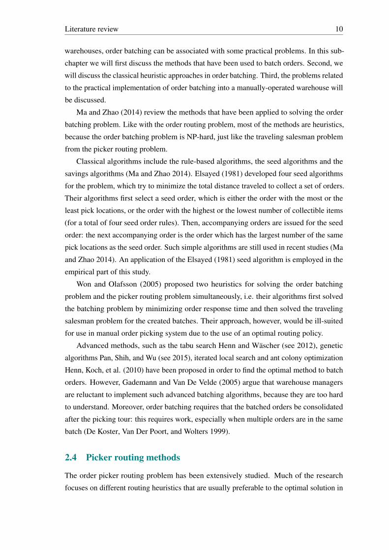
Classical algorithms include the rule-based algorithms, the seed algorithms and the
savings algorithms (Ma and Zhao 2014). Elsayed (1981) developed four seed algorithms
for the problem, which try to minimize the total distance traveled to collect a set of orders.
Their algorithms first select a seed order, which is either the order with the most or the
least pick locations, or the order with the highest or the lowest number of collectible items
(for a total of four seed order rules). Then, accompanying orders are issued for the seed
order: the next accompanying order is the order which has the largest number of the same
pick locations as the seed order. Such simple algorithms are still used in recent studies (Ma
and Zhao 2014). An application of the Elsayed (1981) seed algorithm is employed in the
empirical part of this study.
Won and Olafsson (2005) proposed two heuristics for solving the order batching
problem and the picker routing problem simultaneously, i.e. their algorithms first solved
the batching problem by minimizing order response time and then solved the traveling
salesman problem for the created batches. Their approach, however, would be ill-suited
for use in manual order picking system due to the use of an optimal routing policy.
Advanced methods, such as the tabu search Henn and Wäscher (see 2012), genetic
algorithms Pan, Shih, and Wu (see 2015), iterated local search and ant colony optimization
Henn, Koch, et al. (2010) have been proposed in order to find the optimal method to batch
orders. However, Gademann and Van De Velde (2005) argue that warehouse managers
are reluctant to implement such advanced batching algorithms, because they are too hard
to understand. Moreover, order batching requires that the batched orders be consolidated
after the picking tour: this requires work, especially when multiple orders are in the same
batch (De Koster, Van Der Poort, and Wolters 1999).
2.4 Picker routing methods
The order picker routing problem has been extensively studied. Much of the research
focuses on different routing heuristics that are usually preferable to the optimal solution in
Literature review 11
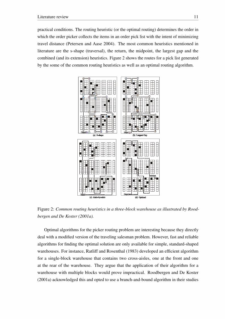
practical conditions. The routing heuristic (or the optimal routing) determines the order in
which the order picker collects the items in an order pick list with the intent of minimizing
travel distance (Petersen and Aase 2004). The most common heuristics mentioned in
literature are the s-shape (traversal), the return, the midpoint, the largest gap and the
combined (and its extension) heuristics. Figure 2 shows the routes for a pick list generated
by the some of the common routing heuristics as well as an optimal routing algorithm.
Figure 2: Common routing heuristics in a three-block warehouse as illustrated by Rood-
bergen and De Koster (2001a).
Optimal algorithms for the picker routing problem are interesting because they directly
deal with a modified version of the traveling salesman problem. However, fast and reliable
algorithms for finding the optimal solution are only available for simple, standard-shaped
warehouses. For instance, Ratliff and Rosenthal (1983) developed an efficient algorithm
for a single-block warehouse that contains two cross-aisles, one at the front and one
at the rear of the warehouse. They argue that the application of their algorithm for a
warehouse with multiple blocks would prove impractical. Roodbergen and De Koster
(2001a) acknowledged this and opted to use a branch-and-bound algorithm in their studies

Literature review 12
concerning warehouses with multiple same-shaped blocks. They, however, conclude that
a branch-and-bound method is not suitable for continuous use due to its computational
time requirements. However, computing power of a PC is much higher today than it was
in the time of the study of Roodbergen and De Koster (2001a). In addition, De Koster,
Le-Duc, and Roodbergen (2007) note that an optimal algorithm might not even exist for
some warehouse layouts. Therefore, advanced methods for finding at least close-to-optimal
routes have been proposed. For instance, Hsieh, Huang, and Huang (2007) used particle
swarm optimization (PSO), a population-based stochastic optimization technique enhanced
with a genetic algorithm to find near-optimal solutions.
Generally, literature discourages the use of optimal routing in manually operated
warehouses not only due to the difficulty of implementing fast and reliable algorithms to
finding the optimal solution in the first place, but also due to the practical problems such
routes could cause. For example, from the order picker’s point of view, it is desirable to
have routes that are simple and easy to understand, which the optimal routes rarely are.
Having simple routes allows the order picker to find the pick locations more easily with
less errors (Roodbergen and De Koster 2001a)). However, some heuristics may also appear
too complicated. For instance, Petersen and Schmenner (1999) argue that a combination
of the s-shape and the largest gap heuristic generates routes so complicated that the order
picker is bound to make mistakes.
Petersen and Schmenner (1999) compared the performance of different routing heuris-
tics with different class-based storage assignments. They argue that if for each scenario,
the best performing routing heuristic were chosen, optimal routing would be only 3.3%
more efficient than the mix of heuristics. Moreover, Caron, Marchet, and Perego (1998)
compared the performance of the s-shape and the return routing methods in different
conditions using the COI. Generally, literature offers no one definite ordering of the heuris-
tics, because their performance is linked to other variables. However, the combined(+)
heuristic introduced by Roodbergen and De Koster (2001a) was the best heuristic in over
90% of their experiments, with the largest gap heuristic coming in at second place in
overall performance. Generally, the best routing heuristic seems to strongly depend on the
stock location assignment strategy (De Koster, Le-Duc, and Roodbergen 2007), e.g. the
within-aisle assignment might be more suitable for the s-shape heuristic than, for instance,
the across-aisle assignment.
Finally, from a general point of view, research on the picker routing problem may be
excessive. Petersen and Aase (2004) show that the benefit from using optimal routing
(or a complicated heuristic) instead of, for instance, the s-shape heuristic is negligible
compared to the benefits from introducing batching procedures or a class-based stock

Literature review 13
location assignment. Therefore, the routing strategy should only be considered after the
storage location assignment and the batching method have been optimized.

Research material and methods 14
3 Research material and methods
For the purpose of optimizing the order picking process in the case DC, we propose a
comprehensive framework addressing the issues that affect order picking efficiency the
most. Based on earlier literature, the most important decisions concerning the order
picking efficiency in manually-operated warehouses were the layout, the storage location
assignment, the order batching method, and the picker routing method, all of which we
discussed in chapter 2. Our empirical framework addresses the last three of these decisions
directly. The first one - the layout - is addressed indirectly via choices made with the picker
routing method. As mentioned earlier, few earlier papers address all of these issues in
real-life scenarios.
In this chapter, we discuss the elements of the framework one-by-one, starting with data
sources and their preparation for the pipeline. Then, we move onto the storage location
assignment, which is split between two phases, order analysis and SKU clustering, and
the actual assignment strategies. After the storage location assignment, we describe the
order batching methods in detail. Then, we describe the picker routing method created for
the DC’s layout. Finally, we conclude this chapter by discussing the framework and its
implementation.
3.1 Data
The data used in this study comprises historical demand data of all the SKUs in the DC
and the layout of the DC. These two data sources are essential for the modeling of the
order picking process. The data also includes the stock level report of the DC containing
information about the SKUs currently in the DC that is used to supplement the demand
data in the modeling phase. According to Bartholdi and Hackman (2011, pp. 231), these
three data sources are needed to model warehouse activity. Modeling the order picking
process of a distribution center accurately is information-intensive. It is imperative that
there is a large supply of historical order data to model the demand of the DCs SKUs
adequately.
Each of the data sources is needed in multiple phases along the pipeline of our frame-
work. For instance, the historical demand data has two main purposes: to order SKUs
based on their demand and to determine their clustering structure. Moreover, the historical
demand data contains information about the SKUs’ batching characteristics which the
batching algorithms make use of. Hence, due to the complexity of the setting, we discuss
each of the data sources separately. We will discuss the data sources and their uses in the
following order: 1) the layout, 2) the stock level report, 3) historical SKU demand and
Research material and methods 15
order pick lists.
3.1.1 The layout
Earlier research has mostly used simple and easy-to-understand warehouse layouts, al-
though it has never been proven that solutions created for them can be generalized for
more complex layouts in a straightforward way. Exceptions to this rule can be found in,
for instance, Pohl, Meller, and Gue (2011) and Dekker et al. (2004): these papers use
more unorthodox layouts. The layout of the case distribution center can be thought of as
a mix of a multi-block warehouse with front and rear cross-aisles, and a warehouse with
a block with only a front cross-aisle. A layout of this shape is not discussed in literature.
Therefore, we had to create a modeling scheme for this particular layout from scratch. A
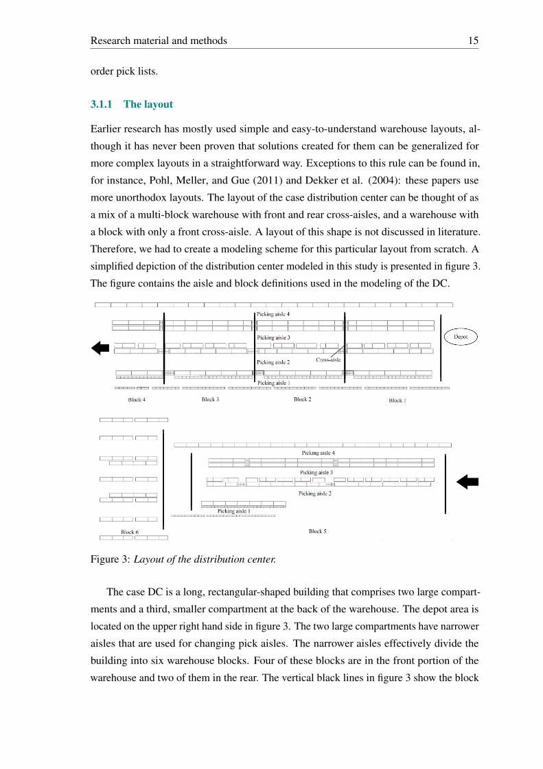
simplified depiction of the distribution center modeled in this study is presented in figure 3.
The figure contains the aisle and block definitions used in the modeling of the DC.
Figure 3: Layout of the distribution center.
The case DC is a long, rectangular-shaped building that comprises two large compart-
ments and a third, smaller compartment at the back of the warehouse. The depot area is
located on the upper right hand side in figure 3. The two large compartments have narrower
aisles that are used for changing pick aisles. The narrower aisles effectively divide the
building into six warehouse blocks. Four of these blocks are in the front portion of the
warehouse and two of them in the rear. The vertical black lines in figure 3 show the block

Research material and methods 16
division. These blocks somewhat differ in size and shape. The six blocks are the basis for
the modified s-shape picker routing method (see 3.5) that is used to estimate route lengths
for order pick lists. The two main compartments have four parallel aisles each. The third,
smaller compartment, however, contains six parallel aisles, which, for practical purposes
were reduced to three in the modeling phase (see 3.5).
The document containing the DC layout is a PDF file, which can be used for the
extraction of the coordinates of individual racks in the DC with great accuracy. In figure 3
depicting the DC, the small rectangles of different sizes represent the individual racks. Each
of these racks has a number of individual stock places. Unique stock places have a unique
identifier code that follows a simple convention, making the identifier easy to manipulate.
The quantities of the unique stock places in each rack is used to create simulated SKU
placements in the DC (see 3.2.2). A single rectangle may contain a few dozen unique stock
places. Therefore, consolidating the stock places into larger units such as single racks (i.e.
rectangles) is the only way to purposefully simulate a SKU location assignment given the
very high number of individual stock place identifiers.
The consolidation process is extremely simple for every stock place in the DC. The
unique stock place identifier code for each stock place contains, among more accurate
location information, information about the rack row of the stock place and its position in
the rack row indicated by a running index. These two pieces of information can be used to
pinpoint a unique stock place identifier to a rack (rectangles in the figures) by modifying
the identifier code with string operations. After the consolidation, we are left with 310 and
212 possible physical locations for the pallet and small SKUs, respectively. This way, only
522 unique coordinates for the stock places are needed. Dekker et al. (2004, pp. 305-306)
employed similar tactics to reduce the number of individual stock places. The physical
sizes (total unique stock place identifiers as a proportion of the total) and the number of
individual coordinates in each block are reported in table 1.
Table 1: Stock place distribution by block.
Block 1 2 3 4 5 6
Stock places (of total) 19.1% 18.7% 17.7% 8.5% 31.2% 4.8%
Total consolidated 86 84 82 45 176 49
We notice that blocks one, two, and three are nearly equal in size. Block four is
considerably smaller, whereas the fifth block in the second large compartment of the DC is
very large compared to the other blocks measured in both metrics. The sixth block in the
back of the DC has very low overall capacity compared to the other blocks. Furthermore,
Research material and methods 17
the rectangles, or the unique racks, may be divided into two classes: pallet racks that may
hold extremely heavy items and racks specifically designed to house small items. The small
item racks (tiny rectangles) are located in the lowest parallel aisle of the warehouse (see
picking aisle 1 in figure 3), whereas all the other racks are pallet racks (larger rectangles).
The distinction between pallet and small item racks makes solving the storage location
assignment problem somewhat harder later on (see 3.2.1). For instance, items that are
small may be placed on the pallet racks but large items may not be placed on the small
item racks.
Evidently, the layout is essential for the picker routing heuristic and the class-based
storage assignment methods. First, the routing heuristic needs distances (derived from
the rack coordinates) so that it can calculate routes according to SKU locations (see 3.5).
Second, zones (see 3.2.2) for the class-based methods are derived straight from the layout,
with the rectangles in figure 3 being divided into zones for the classes. Last, evaluating
different decision combinations would not be possible without the exact layout of the
warehouse. The models used in this study do not use approximations or other methods to
determine the pick locations of SKUs during simulation that are common in older studies,
but stock locations accurate to less than a meter that take into account differences in rack
sizes and types. Taking this approach allows for detailed analysis of different picking
routes later on.
3.1.2 The stock level report
The stock level report may be used to study the distribution of the items in the DC: this
is beneficial when we deploy artificial SKU locations in the storage location assignment
phase. The report is used to assess the utilization rate of different racks of the DC - the
approximation of which in the storage location assignment phase is very hard. Therefore,
it may give insight into the number of SKUs that may be assigned to each zone in the
class-based assignments (see 3.2.1). The report itself is a static document that updates
daily. It contains information about the SKUs that are currently in the warehouse. Most
importantly, it reports some item specific information for each SKU: the type of the item,
its current stock quantity and value - and most importantly - its storage location, i.e. its
stock location identifier.
During data preprocessing (see 3.1.3), the stock level report is used to filter out un-
desirable rows from the demand data. Specifically, demand rows for SKUs that are no
longer present in the warehouse are omitted, because such items have no future expected
demand from the DC and - as such - cannot be used to model the process anymore, and
their inclusion into the analyses would cause inaccuracies.
Research material and methods 18
The stock location report has a large role in the deployment of the model in practice.
During the practical implementation of a proposed model, it is used as the basis for the
lists that suggest changes to the storage location assignment. Specifically, the current SKU
storage locations presented in the stock level report are compared to the locations in the
proposed storage location assignment, which immediately tells the warehouse personnel
whether an SKU is currently located in the correct area or not.
3.1.3 Historical SKU demand and order pick lists
The most critical part of this study is the DC’s event data, because it allows us to define
what has been taken from the warehouse racks. We must determine 1) when an SKU
has been taken from the racks 2) if the SKU was the only pick of the tour or were there
other SKUs picked at the same time 3) what the locations of the order pick lines were
according to the warehouse layout picture. We define an order pick line as a row in the
order describing an SKU to be collected during a single tour. We argue that the demand
data is more crucial than the exact layout picture, because the layout picture could be
approximated via various methods. However, to meaningfully generate storage location
assignments, individual demand data for each of the SKUs in the warehouse is required.
The DC event data is fetched from a database that lists all stock events from every
warehouse of the client firm. The database is located in a cloud-computing environment
from which the required data is extracted via SQL queries. The data set is intricate and
understanding it requires good knowledge of the DC’s bookkeeping rules. For instance,
there is a large number of different stock event types, the use of which is not always
universal across the database. In addition, the meaning of some of the stock events is
unclear without thorough investigation of both the database and the underlying warehouse
process. Therefore, extensive pre-processing of the event data was required to filter out
pure SKU demand data for the DC. The pre-processing mainly concerned data unfit to be
modeled and the different pick operation types. The pre-processing steps were roughly the
following:
1. Find only the data concerning the case DC.
2. Only consider negative stock events: a negative "quantity" value indicates a pick
event.
3. Determine which stock event types can depict pick events (see 4.1 for more informa-
tion).
4. Filter out events that do not involve the order picker moving around the DC.

Research material and methods 19
5. Filter out order pick rows whose SKUs are not currently present in the stock level
report.
After pre-processing, the data is ready to be used to model the system. The procedures
where the processed demand data is used are: 1) ABC analysis (see 3.2) 2) order analysis
(see 3.3) 3) SKU cluster analysis according to the information obtained in step 2 (see
3.3) 4) batching according to the information obtained in step 2 (see 3.4). Moreover, the
pure processed event data may be fed directly into the picker routing algorithm to assess
the current and historical performance of the DC’s order picking efficiency. Finally, the
processed data may be further altered to use simulated storage location assignments to
see, what the order picking efficiency of the warehouse would have been had the location
assignment been different.
The stock event data does not tell us about the structure of the real pick order lists: a
realized picking tour is not necessarily the same as the whole pick list. This could happen
due to e.g. the pick list being too large to be picked in a single tour (multiple tours required
for a single list) or inconsistencies in data input. The extraction of the event lines belonging
to the same tour from the event data was done by grouping lines of a single event type
(pick lists may only contain lines of the same event type) according to their event times:
all lines that have been input to the system with the same timestamp are considered part of
the same picking tour (as soon as a set of pick lines arrives in the depot area, a stock event
is created). This strategy allowed a fairly accurate extraction of the realized pick lists and
their SKUs.
3.2 Class-based storage assignments
The main method of improving the efficiency of the order picking process is the manipula-
tion of the storage location assignment, alongside changing the picker routing and batching
policies. Class-based storage assignments are universally used in many order picking
processes because of their flexibility and ease of implementation. The reasons to employ a
class-based storage with multiple zones in the case DC are numerous:
• The length-to-width ratio of the case DC is very high and the pickers use somewhat
slow vehicles to move around. A totally random assignment is thus discouraged.
• The demand structure of the DC is skewed: a fraction of the SKUs constitute a large
part of the total demand measured in order pick lines.
• More complex methods such as the COI-measure are discouraged because of insuffi-
cient data.

Research material and methods 20
• Literature emphasizes the need for robust location assignment solutions.
• Class-based assignments may be complimented with correlation-based methods.
Next, we will describe how the SKUs were divided into different classes based on
their expected demand. We discuss the generation of the popularity measure for the SKUs.
Second, we will describe three class-zone variants to be used in the simulations. Last, we
will describe the method we used to communicate the proposed class-zone variant to the
DC personnel and how the proposed storage location assignment could be achieved the
easiest and the fastest.
3.2.1 Class generation
The DC contains two different kinds of racks (see 3.1.1): large pallet racks and small
item racks for small SKUs. The two SKU classes have somewhat different demand
characteristics, so we opted to run two parallel demand analyses: one for each of the SKU
types. This approach is endorsed by the fact that all the small SKU racks are located
in a single pick aisle - effectively in their own compartment. This makes the practical
implementation of the proposed models easier, although increasing computational time
by almost a half. These demand analyses are essentially the ABC analyses that were
introduced in 2.2.1.
We defined three classes based on SKU turnover for both the large pallet racks and
the small item racks for a total of six classes. The analysis itself was conducted in the
following manner: 1) determining the time window (how many months of demand data is
used to estimate SKU demand) for the demand data 2) calculating the number of times each
SKU appears in a pick list during the time window 3) sorting the resulting list of SKUs in
a descending order based on the number of pick list occurrences (i.e. SKU demand). Then,
the class divisions were based on the Pareto principle: a small number of unique SKUs
account for the majority of the pick events (see figure 4). To generate classes, we simply
cut the SKU distribution at certain percentiles (of total demand rows). The demand row
percentiles that divide the SKUs in classes were different for the two SKU types pertaining
to the differences in the physical size of the ABC class zones in the DC (see 3.2.2). We
named the three classes the fast, intermediate and slow SKUs. The fast, intermediate and
slow SKUs are divided with black vertical lines in figure 4 with the fast SKUs generating
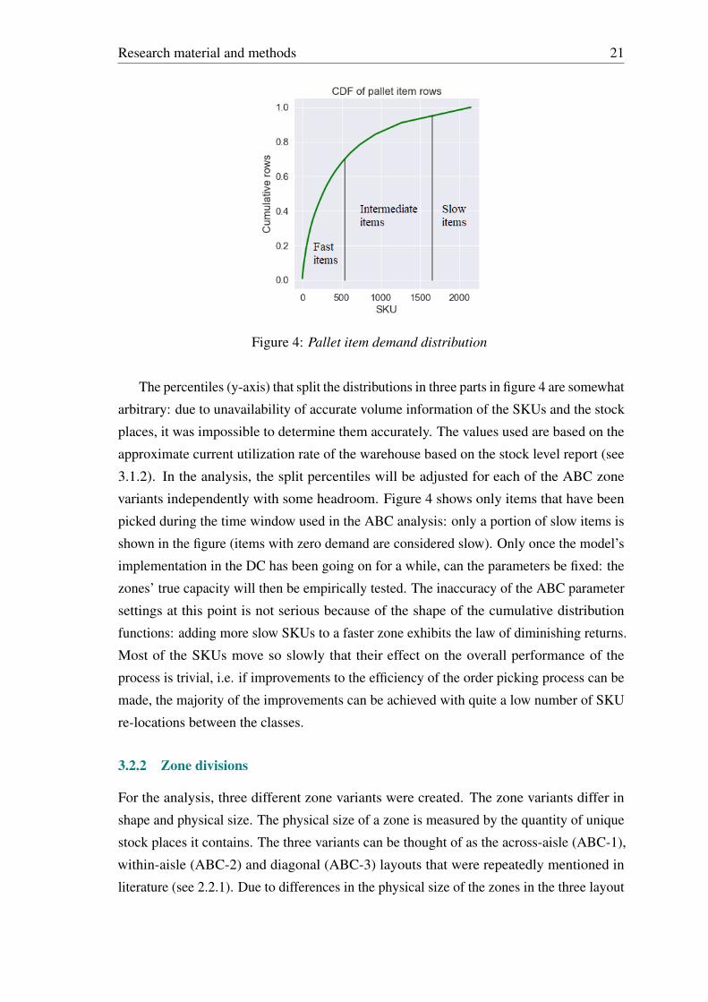
70%, the intermediate SKUs 25% and the slow SKUs 5% of total SKU demand. Figure 4 is
the visualized output of the ABC analysis for the pallet items, where the x-axis reports the
SKU demand rank (descending popularity order), and the y-axis the cumulative number of
order pick lines (total demand) during the time window for the analysis.
Research material and methods 21
Figure 4: Pallet item demand distribution
The percentiles (y-axis) that split the distributions in three parts in figure 4 are somewhat
arbitrary: due to unavailability of accurate volume information of the SKUs and the stock
places, it was impossible to determine them accurately. The values used are based on the
approximate current utilization rate of the warehouse based on the stock level report (see
3.1.2). In the analysis, the split percentiles will be adjusted for each of the ABC zone
variants independently with some headroom. Figure 4 shows only items that have been
picked during the time window used in the ABC analysis: only a portion of slow items is
shown in the figure (items with zero demand are considered slow). Only once the model’s
implementation in the DC has been going on for a while, can the parameters be fixed: the
zones’ true capacity will then be empirically tested. The inaccuracy of the ABC parameter
settings at this point is not serious because of the shape of the cumulative distribution
functions: adding more slow SKUs to a faster zone exhibits the law of diminishing returns.
Most of the SKUs move so slowly that their effect on the overall performance of the
process is trivial, i.e. if improvements to the efficiency of the order picking process can be
made, the majority of the improvements can be achieved with quite a low number of SKU
re-locations between the classes.
3.2.2 Zone divisions
For the analysis, three different zone variants were created. The zone variants differ in
shape and physical size. The physical size of a zone is measured by the quantity of unique
stock places it contains. The three variants can be thought of as the across-aisle (ABC-1),
within-aisle (ABC-2) and diagonal (ABC-3) layouts that were repeatedly mentioned in
literature (see 2.2.1). Due to differences in the physical size of the zones in the three layout
Research material and methods 22
models, the ABC analyses for each of the layouts was run with different split parameters
(see 3.2.1 and figure 4). Figures 5, 6 and 7 show the layouts used in the analysis. In each
figure, the green part of the DC is reserved for the fast moving SKUs, the yellow part for
the intermediate SKUs and the red part for the slow SKUs. The figures do not contain the
rear part (blocks five and six) of the DC presented in figure 3, as it is reserved for the slow
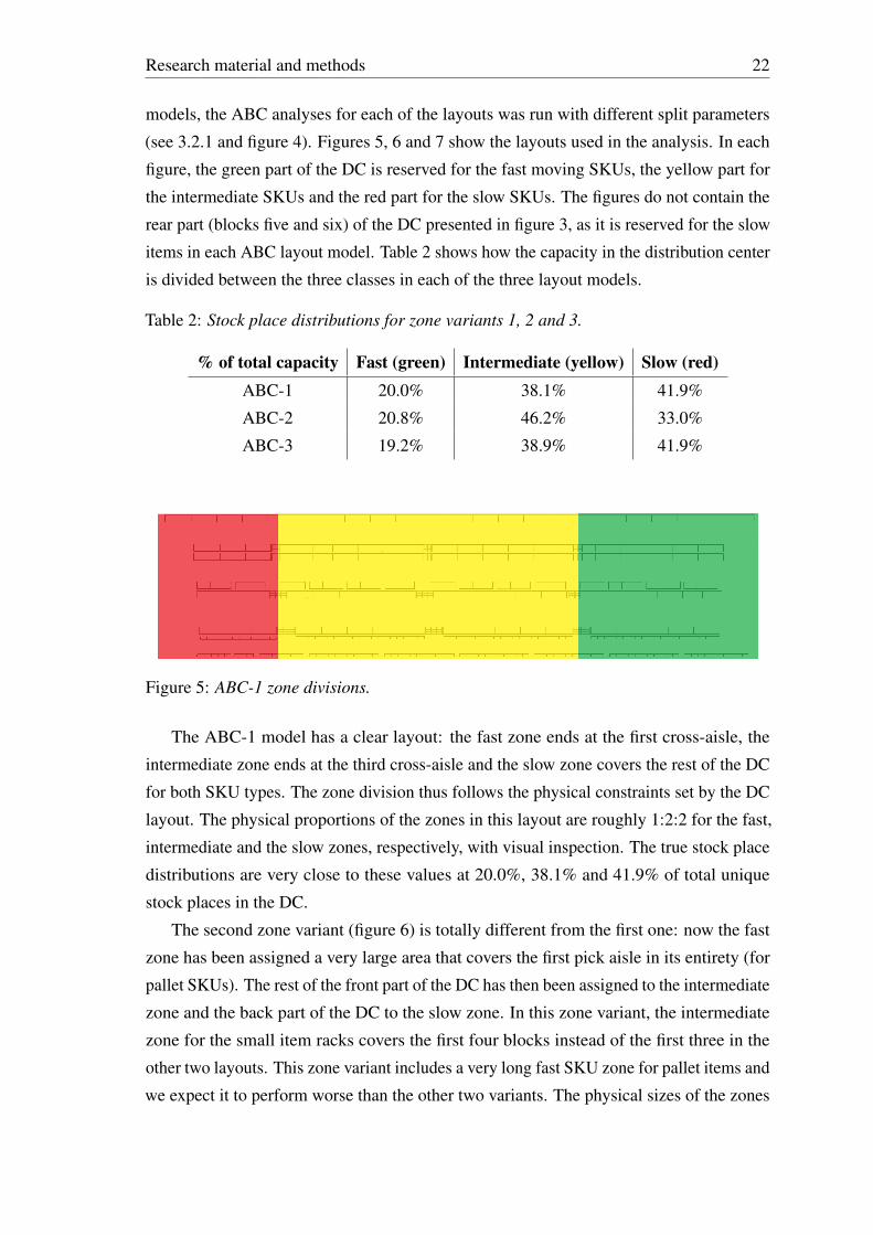
items in each ABC layout model. Table 2 shows how the capacity in the distribution center
is divided between the three classes in each of the three layout models.
Table 2: Stock place distributions for zone variants 1, 2 and 3.
% of total capacity Fast (green) Intermediate (yellow) Slow (red)ABC-1 20.0% 38.1% 41.9%
ABC-2 20.8% 46.2% 33.0%
ABC-3 19.2% 38.9% 41.9%
Figure 5: ABC-1 zone divisions.
The ABC-1 model has a clear layout: the fast zone ends at the first cross-aisle, the
intermediate zone ends at the third cross-aisle and the slow zone covers the rest of the DC
for both SKU types. The zone division thus follows the physical constraints set by the DC
layout. The physical proportions of the zones in this layout are roughly 1:2:2 for the fast,
intermediate and the slow zones, respectively, with visual inspection. The true stock place
distributions are very close to these values at 20.0%, 38.1% and 41.9% of total unique
stock places in the DC.
The second zone variant (figure 6) is totally different from the first one: now the fast
zone has been assigned a very large area that covers the first pick aisle in its entirety (for
pallet SKUs). The rest of the front part of the DC has then been assigned to the intermediate
zone and the back part of the DC to the slow zone. In this zone variant, the intermediate
zone for the small item racks covers the first four blocks instead of the first three in the
other two layouts. This zone variant includes a very long fast SKU zone for pallet items and
we expect it to perform worse than the other two variants. The physical sizes of the zones

Research material and methods 23
Figure 6: ABC-2 zone divisions.
are, however, not that different from the other two variants: now the fast zone includes
20.8%, the intermediate zone 46.2% and the slow zone 33.0% of all stock places.
Figure 7: ABC-3 zone divisions.
The third variant, the ABC-3 (figure 7) is essentially ABC-1 with slight modifications
to the shape of the fast and intermediate pallet zones. It is somewhat similar to the diagonal
ABC layout often mentioned in literature. The triangular zones were created to test whether
there is enough correlation between the small SKU type and the pallet SKU type: the
longer edge of the fast pallet zone lies next to the fast small SKU zone, which allows more
fast SKUs to be placed closer to it. If high demand correlation was present between these
two fast zones, we hypothesized that the ABC-3 model would perform somewhat better
than the ABC-1 model. Although this layout looks curious on paper, in practice it could
be implemented as easily as the two other zone variants. The physical sizes are almost
identical to that of the ABC-3 layout: 19.3%, 38.9% and 41.9% to the fast, intermediate and
slow zones, respectively. Because the physical sizes of the zones in ABC-1 and ABC-3 are
almost identical, we can easily determine, which one of them is more efficient by running
the ABC analyses for them with the same parameters (see 3.2.1) to achieve identical rack
utilization rates for both variants.
3.3 Correlation-based storage assignments
The DC contains thousands of unique SKUs. We define an SKU cluster as a set of SKUs that
are statistically correlated - they are often picked during the same tour. Only a fraction of all

Research material and methods 24
SKUs can be considered part of an SKU cluster, i.e. the overall level of demand correlation
between items in the DC is low. Therefore, creating a storage location assignment for the
whole DC using only SKU clusters is impossible: the clusters must be used to complement
another assignment, namely the class-based ABC assignment, which classifies the SKUs
based on their expected demand. Hence, the storage location assignment method that
exploits SKU correlations will be a combination of the two strategies: the class-based
method will be the main method (random assignment inside zones) in the background,
and a limited number of significant SKU clusters (dedicated assignment) will be located
in the zones. Mixing the two strategies together may cause some problems. However:
1) the number of SKU clusters is very limited, 2) most of the clusters should already be
self-evident for the DC personnel, 3) all clusters will be located in a relatively small area in
the fast moving SKU zones seemingly separate from the random items (see 8). Therefore,
including the cluster assignment into the class-based system should be feasible.
Using clusters alongside the class-based method has two main advantages over the
pure class-based method: in the fast zones, cluster SKUs may be assigned to stock places
adjacent to each other, which reduces the distance the picker needs to travel to collect
all items in a pick list. This is especially useful, when there are many pick aisles in a
zone: random assignments of clusters would lead to much longer travel distances. In such
scenarios: clustering should reduce the number of aisles a picker needs to travel to complete
a tour, on average. During the implementation phase of the new stock location assignment,
the found SKU clusters have another use. If, in the current location assignment, the
SKUs of a cluster are scattered throughout the warehouse, it may be beneficial to schedule
the moving of the SKUs of the cluster such that all of them will be moved to their new
locations subsequently, and the moving will began with the SKU farthest from the depot
area. This will help generate SKU moves that have maximum positive effect on order
picking distances early on in the relocation phase.
Literature discusses many ways to model SKU correlations and a variety of clustering
methods have been developed. Pairwise SKU demand frequencies are the most common
method of modeling SKU correlation. From a practical point of view, these pairwise
frequencies are quite easy to obtain if sufficiently accurate demand data is available.
Specifically, if the SKUs belonging to each picking tour in the warehouse are known, the
pairwise frequencies between SKUs may be calculated. In practise, obtaining the pairwise
frequencies requires computing a square matrix the elements of which show the times
SKU A has been picked together with SKU B during a preset time window. We will call
the elements the pairwise frequencies hereinafter. Depending on the number of the SKUs
that have been demanded during the time window set for finding SKU correlations and the
Research material and methods 25
number of individual pick lists in that window the resulting matrix may be very large and
its generation may be computationally expensive.
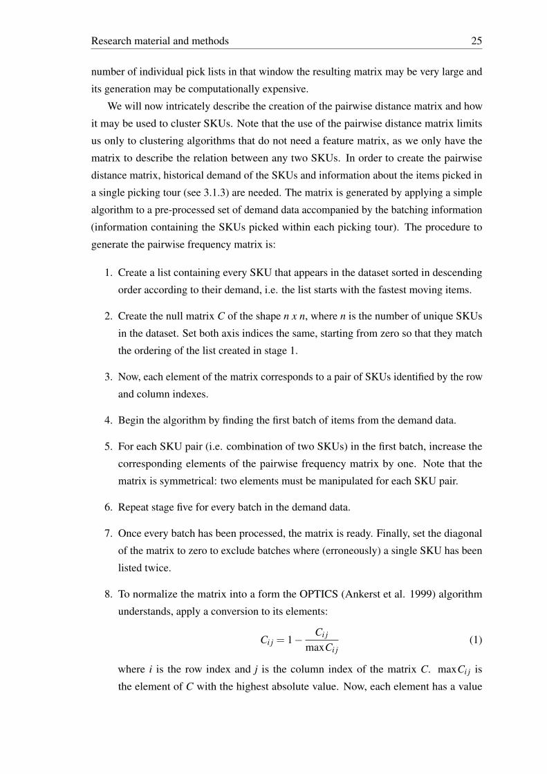
We will now intricately describe the creation of the pairwise distance matrix and how
it may be used to cluster SKUs. Note that the use of the pairwise distance matrix limits
us only to clustering algorithms that do not need a feature matrix, as we only have the
matrix to describe the relation between any two SKUs. In order to create the pairwise
distance matrix, historical demand of the SKUs and information about the items picked in
a single picking tour (see 3.1.3) are needed. The matrix is generated by applying a simple
algorithm to a pre-processed set of demand data accompanied by the batching information
(information containing the SKUs picked within each picking tour). The procedure to
generate the pairwise frequency matrix is:
1. Create a list containing every SKU that appears in the dataset sorted in descending
order according to their demand, i.e. the list starts with the fastest moving items.
2. Create the null matrix C of the shape n x n, where n is the number of unique SKUs
in the dataset. Set both axis indices the same, starting from zero so that they match
the ordering of the list created in stage 1.
3. Now, each element of the matrix corresponds to a pair of SKUs identified by the row
and column indexes.
4. Begin the algorithm by finding the first batch of items from the demand data.
5. For each SKU pair (i.e. combination of two SKUs) in the first batch, increase the
corresponding elements of the pairwise frequency matrix by one. Note that the
matrix is symmetrical: two elements must be manipulated for each SKU pair.
6. Repeat stage five for every batch in the demand data.
7. Once every batch has been processed, the matrix is ready. Finally, set the diagonal
of the matrix to zero to exclude batches where (erroneously) a single SKU has been
listed twice.
8. To normalize the matrix into a form the OPTICS (Ankerst et al. 1999) algorithm
understands, apply a conversion to its elements:
Ci j = 1−Ci j
maxCi j(1)
where i is the row index and j is the column index of the matrix C. maxCi j is
the element of C with the highest absolute value. Now, each element has a value

Research material and methods 26
between zero and one. Values closer to zero indicate an SKU pairing with higher
importance. The OPTICS algorithm that will be applied to this matrix will consider
the SKUs based on these pairwise distance values. For the sum-seed algorithm, this
normalization is not necessary, because the algorithm works purely on the absolute
pairwise frequencies. A partial pairwise frequency matrix used in SKU clustering
can be found in Appendix A.
In the program code (when cluster assignments are used), the cluster SKUs are assigned
stock places very close to each other and all the clusters are located next to each other in
the fast moving SKU zones (see purple racks in figure 8). The clusters are located in the
same racks in all three ABC layouts. When items belonging to clusters have been assigned
storage locations, the rest of the SKUs belonging to the zone will be assigned to the zone
randomly. If there are some non-fast-moving SKUs in the clusters, the same number of
fast-moving non-cluster SKUs will be pushed to the slower intermediate zone (and the
same number of SKUs from the intermediate area to the slow area). Thus, the cluster
assignment used in this thesis gives intermediate or even slow moving SKUs belonging to a
cluster greater importance than to fast moving SKUs that have no measurable relationship
with other SKUs.
Figure 8: The ABC-1 assignment with the cluster assignment.
Next, we will introduce the clustering algorithms that were used to find correlated
itemsets for the storage location assignments. We used multiple algorithms to double check
that the they were working as supposed. In addition to the two algorithms described next,
we also experimented with the apriori algorithm commonly used in market basket analysis,
k-means clustering, and the DBSCAN algorithm. Those algorithms proved vastly inferior
compared to the OPTICS and sum-seed algorithms, when it came to finding meaningful
SKU clusters from the quite sparse data set. For instance, the apriori did indeed find
the most common item sets from the data, but also returned dozens of slightly different
variations for those sets. Moreover, the DBSCAN algorithm seemed to find meaningful
clusters, but it was found out that it would not accept SKUs of differing demands into the
same cluster. The OPTICS and the sum-seed algorithms, however, were able to include

Research material and methods 27
items with different turnover rates into clusters, making them far superior to the other
options.
3.3.1 OPTICS
Ordering of the points to identify the clustering structure or OPTICS is a density-based
clustering algorithm proposed by Ankerst et al. (1999). It is a generalization of the DB-
SCAN (short for density-based spectral clustering for applications with noise) algorithm.
A major benefit of OPTICS compared to e.g. DBSCAN or K-means clustering is that
it is able to extract clusters which include members of differing densities, i.e. in this
case it is better at finding SKU clusters that have both high and low turnover items. The
OPTICS implementation used in this study is the one found in the "Cluster" library of the
scikit-learn machine learning package for Python.
Because there is large variation in the demand frequencies between the SKUs in the
DC’s demand data, OPTICS will outperform most other clustering techniques. Another
benefit of the algorithm is that its parameter setting is simple: setting the noise threshold is
easy, i.e. a single parameter controls the "difficulty" of an SKU entering a cluster. Appendix
B shows the so-called reachability plot for the SKUs included in the cluster analysis. The
algorithm searches for SKU clusters in the valleys between any two higher-reaching points
in the reachability plot.
Due to the nature of the SKU demand data, the algorithm needed to be run twice
for different pick event types. Altogether, the algorithm was able to find a couple dozen
meaningful SKU clusters of differing sizes and with SKUs with different demands. OPTICS
does not limit the size of the clusters it finds, but a lower limit must be set: in this case it
was set at three SKUs. The largest clusters include approximately fifty SKUs, whereas the
smallest meaningful SKUs include three. The algorithm lists the clusters based on their
relevancy: the first few clusters are large and their SKUs all have relatively large demands.
Then the clusters keep getting smaller or the demands of their members start getting smaller,
implying weaker relationships between SKUs. This feature is very important since the
more important clusters constitute a very large part of the total SKU demand rows. A
threshold was set such that the algorithm finds a large number of clusters so as not to
exclude any meaningful ones. During the implementation phase the clusters near the
end of the list provided by the algorithm may then easily be discarded as non-significant.
Such non-significant clusters may, for instance, contain three SKUs but only a handful of
demand lines in total, i.e. it would be more beneficial to consider these items as not being
part of any cluster at all.
Research material and methods 28
3.3.2 Sum-seed algorithm
Zhang (2016) proposes two simple algorithms to cluster SKUs based on their pairwise
demand frequencies. They propose the static-seed and the sum-seed algorithms, which use
very simple procedures to extract clusters from the SKU demand data. This is appealing
for practical purposes as the algorithms can be written in only a few rows, calculate fast
and perform reasonably well. The sum-seed algorithm tries to create clusters one after
another based on the pairwise frequency values the current seed has with all the other
SKUs currently left in the pairwise frequency matrix.
The sum-seed algorithms works in the following way (see Zhang 2016, pp. 32)):
1. Generate the pairwise frequency matrix as described in 3.3. Do not normalize it.
2. Find the fastest moving SKU from the list containing the SKUs in a descending
popularity order and add it to a new cluster. Remove it from the popularity list. The
SKU becomes the seed.
3. Filter the rows of the pairwise frequency matrix with the seed. Locate the the SKU
with the highest pairwise frequency with the seed and add it to the cluster if the
maximum pairwise frequency is higher than a preset threshold value. If no such
SKU is found, end the algorithm and remove the seed from the pairwise frequency
matrix’s rows and columns.
4. If a suitable SKU is found and added to the cluster, the seed is modified: the seed
now contains all the SKUs added to the cluster at this point.
5. Similarly to part three, find the SKU with the highest pairwise frequency with the
seed. When there are multiple SKUs in the cluster already, find the SKU with the
highest aggregate pairwise frequency value with the seed and add it to the cluster.
The algorithm ends if: 1) no SKU satisfying the minimum threshold can be found 2)
the cluster has exceeded the preset value of maximum SKUs allowed in a cluster.
6. Once the cluster is complete, delete its members from the popularity list and the
rows and the columns of the pairwise frequency matrix.
7. Again, find the fastest remaining SKU from the popularity list and repeat the process
sufficiently many times. An upper limit to the number of times a new cluster will be
created should be set so that the algorithm does not iterate the whole SKU popularity
list: meaningful clusters should be found relatively early on.

Research material and methods 29
3.4 Order batching
Once the storage location assignment has been set according to any of the strategies
described earlier, order batching will take place in our framework. In this study, we will
apply two simple algorithms for this problem according to the DC’s restrictions, in addition
to the scenario where no batching is applied at all (FCFS - the first come, first served
method). The two algorithms are a seed algorithm exploiting storage location dependencies
between orders and an algorithm that generates random batches. Next, we describe the
general rules and restrictions used when batching orders, after which the two algorithms
will be described in greater detail.
The WMS (warehouse management system) of the DC receives orders during all times
of the day. To apply batching to these orders, they must be pooled by some criteria. In
the case DC, customer orders are typically printed twice a day, in the morning and in the
afternoon. Because most orders are usually printed at fixed intervals, a fixed time window
batching method should be used to batch orders. In fixed time window batching, incoming
orders are pooled at certain points of time after which they will be batched with some
method. Therefore, we chose to use a pooling method that essentially splits each 24-hour
period in two parts: a six-hour period starting at 09:00 and ending at 15:00 in the afternoon
and an 18-hour period starting at 15:00 and ending at 09:00 the next morning. Pools will
accumulate orders during these time windows and the pools will be batched for picking
once the window ends.
For practicality reasons, the order arrival times are approximated by the event times
which indicate that the orders have been completed. Orders are primarily collected with
the FCFS method in the current system, which means that the orders should leave the DC
in approximately the same order in which they arrived in the WMS. The main reason for
using this proxy for the arrival times is that the real order arrival times cannot be extracted
from the database in a consistent manner in the scope of this study, whereas the event times
for the outgoing orders are known for each pick line.
Furthermore, to conduct batching, restrictions to the picker’s capacity must be set: a
limit for the number of items the order picker is able to collect during a same tour must be
determined. Because the DC contains items of differing physical sizes, estimation of this
parameter is hard and some approximations are required. An order may contain items from
the small item racks only, from the pallet item racks only, or from both of them. Therefore,
it should be possible to find a relationship between these two item types by analyzing
orders that utilize the picker’s capacity to the fullest. Figure 9 shows the scatter plot of
pallet item lines and small item lines. Some of the points are superimposed, meaning that
a single point may include multiple different orders having the same number of small and
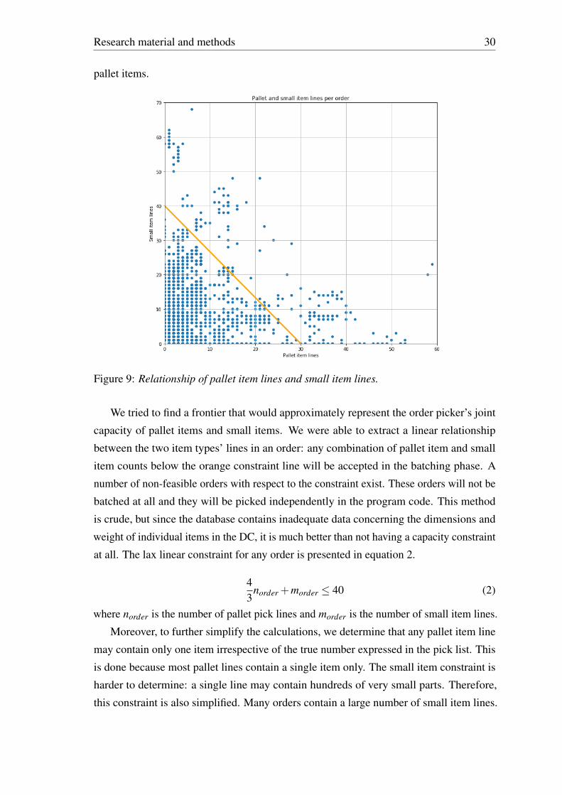
Research material and methods 30
pallet items.
Figure 9: Relationship of pallet item lines and small item lines.
We tried to find a frontier that would approximately represent the order picker’s joint
capacity of pallet items and small items. We were able to extract a linear relationship
between the two item types’ lines in an order: any combination of pallet item and small
item counts below the orange constraint line will be accepted in the batching phase. A
number of non-feasible orders with respect to the constraint exist. These orders will not be
batched at all and they will be picked independently in the program code. This method
is crude, but since the database contains inadequate data concerning the dimensions and
weight of individual items in the DC, it is much better than not having a capacity constraint
at all. The lax linear constraint for any order is presented in equation 2.
43
norder +morder ≤ 40 (2)
where norder is the number of pallet pick lines and morder is the number of small item lines.
Moreover, to further simplify the calculations, we determine that any pallet item line
may contain only one item irrespective of the true number expressed in the pick list. This
is done because most pallet lines contain a single item only. The small item constraint is
harder to determine: a single line may contain hundreds of very small parts. Therefore,
this constraint is also simplified. Many orders contain a large number of small item lines.
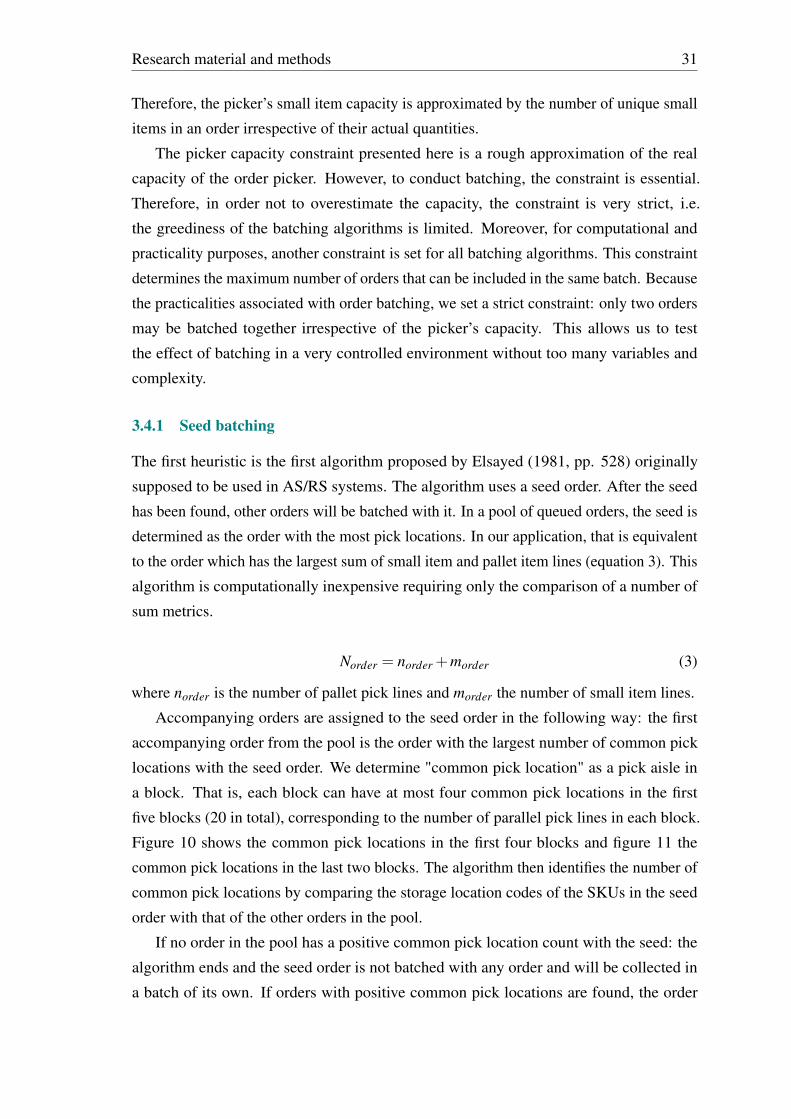
Research material and methods 31
Therefore, the picker’s small item capacity is approximated by the number of unique small
items in an order irrespective of their actual quantities.
The picker capacity constraint presented here is a rough approximation of the real
capacity of the order picker. However, to conduct batching, the constraint is essential.
Therefore, in order not to overestimate the capacity, the constraint is very strict, i.e.
the greediness of the batching algorithms is limited. Moreover, for computational and
practicality purposes, another constraint is set for all batching algorithms. This constraint
determines the maximum number of orders that can be included in the same batch. Because
the practicalities associated with order batching, we set a strict constraint: only two orders
may be batched together irrespective of the picker’s capacity. This allows us to test
the effect of batching in a very controlled environment without too many variables and
complexity.
3.4.1 Seed batching
The first heuristic is the first algorithm proposed by Elsayed (1981, pp. 528) originally
supposed to be used in AS/RS systems. The algorithm uses a seed order. After the seed
has been found, other orders will be batched with it. In a pool of queued orders, the seed is
determined as the order with the most pick locations. In our application, that is equivalent
to the order which has the largest sum of small item and pallet item lines (equation 3). This
algorithm is computationally inexpensive requiring only the comparison of a number of
sum metrics.
Norder = norder +morder (3)
where norder is the number of pallet pick lines and morder the number of small item lines.
Accompanying orders are assigned to the seed order in the following way: the first
accompanying order from the pool is the order with the largest number of common pick
locations with the seed order. We determine "common pick location" as a pick aisle in
a block. That is, each block can have at most four common pick locations in the first
five blocks (20 in total), corresponding to the number of parallel pick lines in each block.
Figure 10 shows the common pick locations in the first four blocks and figure 11 the
common pick locations in the last two blocks. The algorithm then identifies the number of
common pick locations by comparing the storage location codes of the SKUs in the seed
order with that of the other orders in the pool.
If no order in the pool has a positive common pick location count with the seed: the
algorithm ends and the seed order is not batched with any order and will be collected in
a batch of its own. If orders with positive common pick locations are found, the order

Research material and methods 32
Figure 10: The 16 common pick locations in the first four blocks of the DC.
Figure 11: The five common pick locations in the last two blocks of the DC.
with the largest common pick location count is merged with the seed order and the merged
order becomes the seed. The seed is updated as long as orders with common pick locations
with the seed are found, or until the picker’s capacity is reached. This is, however, trivial,
as the maximum number of orders in a batch was set at two: a single seed order may only
get one accompanying order. This procedure is continued until all the orders in the pool
have been batched, after which the algorithm moves onto the next pool (time window).
3.4.2 Random batching
The second and final batching method is an algorithm that randomly pairs orders inside a
pool until the pool has been depleted. The random algorithm is used to validate the results
obtained from the FCFS method (no batching at all) and the seed method. Obviously, if
the seed method fails to perform significantly better than the random algorithm, there is no
reason to implement the seed algorithm explained above, but to use an altogether different
approach to order batching. The random algorithm employed here works in the following
way:
1. Inside a fixed time window pool, all order combinations of one and two orders are
enumerated.
2. Combinations that break the picker’s capacity constraint are removed with the ex-

Research material and methods 33
ception of such combinations with the length of one order.
3. A combination of orders is randomly picked from the pool and saved: all combina-
tions containing the orders in this combination will be removed from the pool.
4. This is continued until the pool is empty and all the orders in the pool have been
collected.
3.5 Picker routing with modified s-shape heuristic
The s-shape heuristic is perhaps the most well-known and most implemented heuristic used
in manual order picking operations. The heuristic is intuitive and creates simple routes, as
opposed to some of the more complicated heuristics. As of writing this thesis, the case DC
uses a picker routing system where an order pick list is printed from the ERP system. The
pick list contains all the pick lines sorted by the stock places of the list items in alphabetical
(each letter denoting a row of racks) order. This is a very simple heuristic that closely
resembles the s-shape heuristic. It, however, has some severe limitations concerning the
DC’s block structure and the rack sorting order. Therefore, we opted to use a modified
s-shape implementation that supports multiple blocks and accommodates a non-standard
rear block. The heuristic itself is largely based on the description given by Roodbergen
and De Koster (2001a). Next, an accurate description of the heuristic is given alongside a
depiction of the possible transitions the order picker may make in the warehouse.
The warehouse layout dictates that the heuristic should have four pick aisles in the first
five blocks (see the parallel black lines in figures 12 and 13). However, the sixth block is
shaped differently: it has three single-file racks, which are problematic since we cannot
know which side the picker will pick the items from. Therefore, we simplified the layout in
the last block by allowing the virtual picker to travel through the single-file racks, reducing
the number of the parallel pick aisles in the last block to three. This simplification is shown
in figure 13. Now the order picker collects items from multiple racks in the new virtual
pick aisles at the same time. This choice somewhat reduces the accuracy of the heuristic in
the last block. This reduction in accuracy is, however, not at all critical. First, very few
items are ever fetched from the last block in practice. Second, when items are fetched from
the last block, it is very unusual that more than one aisle needs to be visited during a single
tour.
The algorithm written for this study works in the following way (mostly along the
description for the s-shape heuristic for warehouses with multiple cross aisles given by
Roodbergen and De Koster (2001a, pp. 3-4). Figure 14 contains an example route generated
by this algorithm with picks in the front part of the DC only.

Research material and methods 34
Figure 12: Picker routes in the four first blocks of the DC. The depot is marked with a
black circle.
Figure 13: Picker routes in the two rear blocks of the DC.
1. Determine the leftmost (when viewed from the depot area) pick aisle containing
picks.
2. Move to the front of this leftmost aisle.
3. Determine the farthest block that contains picks.
4. Following the leftmost pick aisle, move to the front cross aisle of the farthest picking
block.
5. Now, determine which of the pick aisles right of the leftmost pick aisle in the farthest
block contain picks.
6. Along the cross aisle, move to the front of the first such aisle. If the current aisle
contains picks, do not move.
7. Now, there are two options. If the current aisle is the only aisle containing picks in
the block, go to the farthest pick location along that parallel pick aisle and return
to the front of the block (this block has now been completely picked). If the block
contains more than one pick aisle, traverse the entire block. Then find the next aisle
containing picks and entirely traverse it to return to the front of the block.

Research material and methods 35
8. Repeat step 7 until all the aisles of the block have been picked. Now, the farthest
block has been handled.
9. Depending on the location of the farthest block, a number of blocks must be handled
before the picker can return to the depot. All the blocks are picked in the same
manner as the farthest block with the picker ending up in front of the block when it
has been completed.
10. The order (left to right or right to left) in which the picker handles each block is
determined by the aisle the picker stops when the previous block has been completed.
The picker always starts the next block by moving to the leftmost or rightmost
back cross aisle with picks in that block, whichever is closest to the aisle the picker
stopped after finishing the previous block.
11. Once the picker arrives at the first block from the depot, the block is picked as usual,
after which the picker returns to the depot and the route is complete.
Figure 14: Example route generated by the s-shape algorithm.
3.6 Framework
Our framework is used to model the order picking process from the moment an order arrives
in the WMS until it has been dispatched from the DC. Essentially, it attempts to model
the order picking process by converting it into a chain of events that contains separate
phases - each of which has its own set of sub-decisions and parameter sets. The practical
implementation of the framework for this study was completely written in the programming
language Python with the necessary data being extracted from various databases. Figure
15 shows the outline of the framework.
The framework includes five distinct phases: 1) data preparation, 2) order analysis and
clustering, 3) storage location assignment, 4) order batching, 5) travel distance calculation.
The relationships between the parts of the model are presented with arrows. The framework
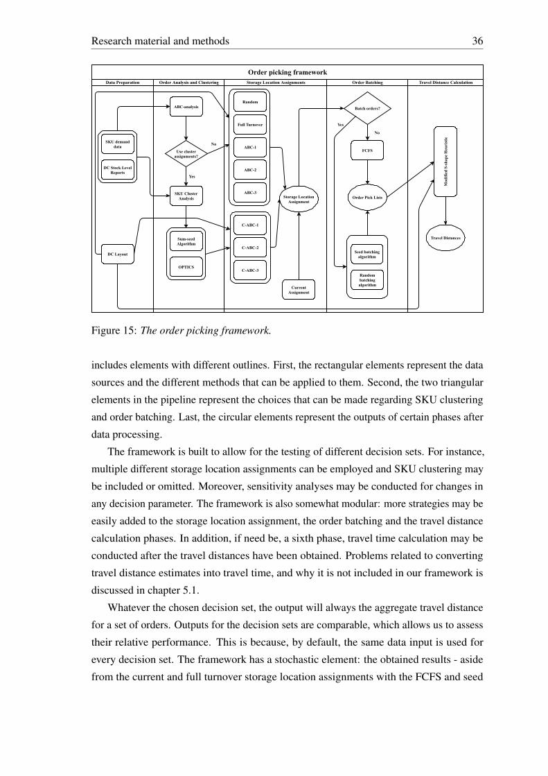
Research material and methods 36
OrderpickingframeworkDataPreparation
DCStockLevelReports
DCLayout
SKUdemanddata
OrderAnalysisandClustering
OPTICS
Sum-seedAlgorithm
ABC-analysis
Useclusterassignments?
SKUClusterAnalysis
Yes
No
StorageLocationAssignments
Random
ABC-2
ABC-1
FullTurnover
ABC-3
C-ABC-1
C-ABC-3
C-ABC-2
StorageLocationAssignment
CurrentAssignment
OrderBatching
Yes
Randombatchingalgorithm
Seedbatchingalgorithm
Batchorders?
OrderPickLists
FCFS
No
TravelDistanceCalculation
TravelDistances
ModifiedS-shapeHeuristic
Figure 15: The order picking framework.
includes elements with different outlines. First, the rectangular elements represent the data
sources and the different methods that can be applied to them. Second, the two triangular
elements in the pipeline represent the choices that can be made regarding SKU clustering
and order batching. Last, the circular elements represent the outputs of certain phases after
data processing.
The framework is built to allow for the testing of different decision sets. For instance,
multiple different storage location assignments can be employed and SKU clustering may
be included or omitted. Moreover, sensitivity analyses may be conducted for changes in
any decision parameter. The framework is also somewhat modular: more strategies may be
easily added to the storage location assignment, the order batching and the travel distance
calculation phases. In addition, if need be, a sixth phase, travel time calculation may be
conducted after the travel distances have been obtained. Problems related to converting
travel distance estimates into travel time, and why it is not included in our framework is
discussed in chapter 5.1.
Whatever the chosen decision set, the output will always the aggregate travel distance
for a set of orders. Outputs for the decision sets are comparable, which allows us to assess
their relative performance. This is because, by default, the same data input is used for
every decision set. The framework has a stochastic element: the obtained results - aside
from the current and full turnover storage location assignments with the FCFS and seed

Research material and methods 37
batching strategies (four in total) - are nondeterministic, meaning that the output itself is
fundamentally a random variable. It is later shown that the standard errors of the output
values are negligible for all stock assignments due to a sufficiently large sample size.
In addition to the scalar-valued output, the framework is built in a way that allows
the construction of time series for assessing the performance of different decision sets
over time. This is especially useful for practical purposes, for instance, keeping track of
the current efficiency level of the DC compared to a simulated decision set. Moreover,
such time series may be used to detect, for instance, seasonalities and differences in order
picking workloads and efficiencies in the DC at different times (e.g. day cycles).
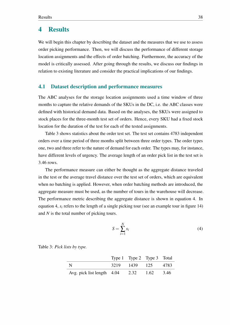
Results 38
4 Results
We will begin this chapter by describing the dataset and the measures that we use to assess
order picking performance. Then, we will discuss the performance of different storage
location assignments and the effects of order batching. Furthermore, the accuracy of the
model is critically assessed. After going through the results, we discuss our findings in
relation to existing literature and consider the practical implications of our findings.
4.1 Dataset description and performance measures
The ABC analyses for the storage location assignments used a time window of three
months to capture the relative demands of the SKUs in the DC, i.e. the ABC classes were
defined with historical demand data. Based on the analyses, the SKUs were assigned to
stock places for the three-month test set of orders. Hence, every SKU had a fixed stock
location for the duration of the test for each of the tested assignments.
Table 3 shows statistics about the order test set. The test set contains 4783 independent
orders over a time period of three months split between three order types. The order types
one, two and three refer to the nature of demand for each order. The types may, for instance,
have different levels of urgency. The average length of an order pick list in the test set is
3.46 rows.
The performance measure can either be thought as the aggregate distance traveled
in the test or the average travel distance over the test set of orders, which are equivalent
when no batching is applied. However, when order batching methods are introduced, the
aggregate measure must be used, as the number of tours in the warehouse will decrease.
The performance metric describing the aggregate distance is shown in equation 4. In
equation 4, si refers to the length of a single picking tour (see an example tour in figure 14)
and N is the total number of picking tours.
S =N
∑i=1
si (4)
Table 3: Pick lists by type.
Type 1 Type 2 Type 3 Total
N 3219 1439 125 4783
Avg. pick list length 4.04 2.32 1.62 3.46
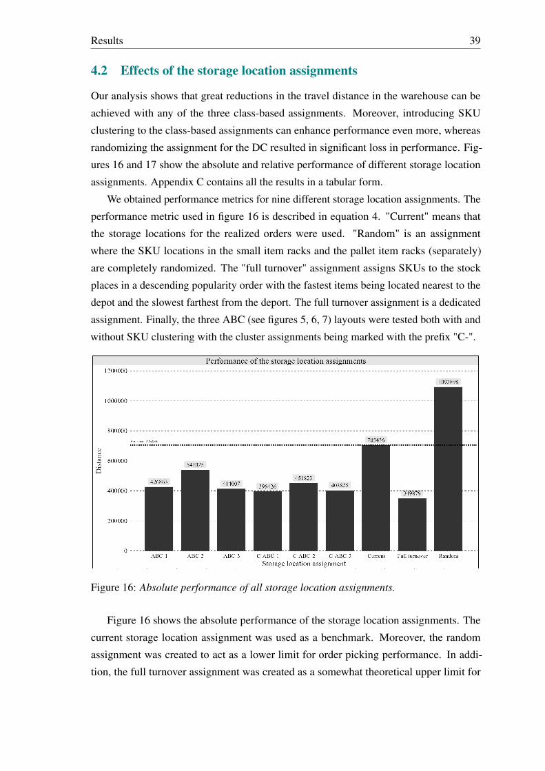
Results 39
4.2 Effects of the storage location assignments
Our analysis shows that great reductions in the travel distance in the warehouse can be
achieved with any of the three class-based assignments. Moreover, introducing SKU
clustering to the class-based assignments can enhance performance even more, whereas
randomizing the assignment for the DC resulted in significant loss in performance. Fig-
ures 16 and 17 show the absolute and relative performance of different storage location
assignments. Appendix C contains all the results in a tabular form.
We obtained performance metrics for nine different storage location assignments. The
performance metric used in figure 16 is described in equation 4. "Current" means that
the storage locations for the realized orders were used. "Random" is an assignment
where the SKU locations in the small item racks and the pallet item racks (separately)
are completely randomized. The "full turnover" assignment assigns SKUs to the stock
places in a descending popularity order with the fastest items being located nearest to the
depot and the slowest farthest from the deport. The full turnover assignment is a dedicated
assignment. Finally, the three ABC (see figures 5, 6, 7) layouts were tested both with and
without SKU clustering with the cluster assignments being marked with the prefix "C-".
Figure 16: Absolute performance of all storage location assignments.
Figure 16 shows the absolute performance of the storage location assignments. The
current storage location assignment was used as a benchmark. Moreover, the random
assignment was created to act as a lower limit for order picking performance. In addi-
tion, the full turnover assignment was created as a somewhat theoretical upper limit for

Results 40
performance: a dedicated full turnover assignment should yield better results than any
class-based assignment. This is clearly indicated in figure 16.
Figure 17: Relative performance of all storage location assignments.
The relative performance of the storage location assignments is shown in figure 17.
The full turnover assignment had the best performance, as expected, improving the current
assignment by approximately 50%. The second best performance was shown by the cluster
variants C-ABC-1 and C-ABC-3, indicating that significant clusters could be obtained
from the demand data. Thus, the assumption that performance would increase if cluster
items were placed close to each other and the clusters close to the loading area held. The
clustered versions of ABC-1 and ABC-3 were quite close to the full turnover assignment
in performance at over 40% reduction in total travel distance compared to the current
assignment. The benefit from using the C-ABC-1 and C-ABC-3 instead of ABC-1 and
ABC-3 was significant.
The ABC-2 assignment achieved considerable reductions in average travel distance at
about 23%. However, its performance was not as nearly as good as that of ABC-1 or ABC-3.
However, When clustering was applied to the ABC-2 assignment, its performance improved
dramatically. At 36% increase in performance compared to the current assignment the
C-ABC-2 assignment approached the ABC-1 in performance. The large increase in
performance can be explained by the large size of the fast pallet item zone in the ABC-2
model: the non-cluster version shares all the fast items uniformly around the long aisle,
whereas the C-ABC-2 allows us to place most of the fastest items very close to the depot
within the cluster zone (see figure 8).
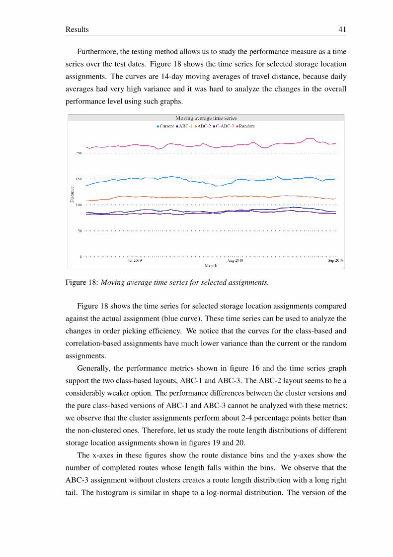
Results 41
Furthermore, the testing method allows us to study the performance measure as a time
series over the test dates. Figure 18 shows the time series for selected storage location
assignments. The curves are 14-day moving averages of travel distance, because daily
averages had very high variance and it was hard to analyze the changes in the overall
performance level using such graphs.
Figure 18: Moving average time series for selected assignments.
Figure 18 shows the time series for selected storage location assignments compared
against the actual assignment (blue curve). These time series can be used to analyze the
changes in order picking efficiency. We notice that the curves for the class-based and
correlation-based assignments have much lower variance than the current or the random
assignments.
Generally, the performance metrics shown in figure 16 and the time series graph
support the two class-based layouts, ABC-1 and ABC-3. The ABC-2 layout seems to be a
considerably weaker option. The performance differences between the cluster versions and
the pure class-based versions of ABC-1 and ABC-3 cannot be analyzed with these metrics:
we observe that the cluster assignments perform about 2-4 percentage points better than
the non-clustered ones. Therefore, let us study the route length distributions of different
storage location assignments shown in figures 19 and 20.
The x-axes in these figures show the route distance bins and the y-axes show the
number of completed routes whose length falls within the bins. We observe that the
ABC-3 assignment without clusters creates a route length distribution with a long right
tail. The histogram is similar in shape to a log-normal distribution. The version of the

Results 42
Figure 19: ABC-3 route length distribution.
Figure 20: C-ABC-3 route length distribution.
ABC-3 assignment employing SKU clustering has a somewhat better overall performance.
However, this assignment seems to create a very large number of routes of similar length as
indicated by the few very frequent bins. This is due to the placement of the SKU clusters
in the front portion of the small item and the first pallet item pick aisles. Implications of
deciding to implement a cluster assignment alongside the pure ABC assignment will be
discussed in 5.1 and 5.2.
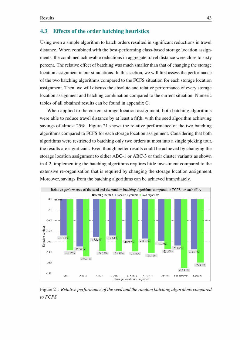
Results 43
4.3 Effects of the order batching heuristics
Using even a simple algorithm to batch orders resulted in significant reductions in travel
distance. When combined with the best-performing class-based storage location assign-
ments, the combined achievable reductions in aggregate travel distance were close to sixty
percent. The relative effect of batching was much smaller than that of changing the storage
location assignment in our simulations. In this section, we will first assess the performance
of the two batching algorithms compared to the FCFS situation for each storage location
assignment. Then, we will discuss the absolute and relative performance of every storage
location assignment and batching combination compared to the current situation. Numeric
tables of all obtained results can be found in appendix C.
When applied to the current storage location assignment, both batching algorithms
were able to reduce travel distance by at least a fifth, with the seed algorithm achieving
savings of almost 25%. Figure 21 shows the relative performance of the two batching
algorithms compared to FCFS for each storage location assignment. Considering that both
algorithms were restricted to batching only two orders at most into a single picking tour,
the results are significant. Even though better results could be achieved by changing the
storage location assignment to either ABC-1 or ABC-3 or their cluster variants as shown
in 4.2, implementing the batching algorithms requires little investment compared to the
extensive re-organisation that is required by changing the storage location assignment.
Moreover, savings from the batching algorithms can be achieved immediately.
Figure 21: Relative performance of the seed and the random batching algorithms compared
to FCFS.

Results 44
When combined with different storage location assignments, the effects of the batching
heuristics differed somewhat. The ABC-2, random and full turnover assignments benefited
the most from using the seed algorithm, with the random and full turnover assignments
saving 30% and 32% over their non-batched versions, respectively. The ABC-2 assignment
improved by 27% when using the seed algorithm, which is notably more than that any of
the other class-based assignments, including the clustered version of ABC-2.
The two assignments benefiting the most from the random batching algorithm were
the ABC-2 and the random storage location assignment. Overall, the performance of the
random algorithm was significantly worse than that of the seed algorithm: none of the
assignments were improved by more than 24% (the random assignment), and the only
class-based assignment that improved by more than 20% was the ABC-2 assignment.
Figure 22 shows the relative performance of every batching and storage location
assignment combination. The bolded labels show the relative performance of the seed
batching algorithm with each of the storage location assignments compared to the current
situation (current FCFS).
Figure 22: Relative performance of all batching and storage location assignment combina-
tions.
When assessing the total savings of the batching and location assignment combinations,
we find out that the most beneficial combination is the seed algorithm combined with the
full turnover assignment, which could potentially reduce travel distance by 66%. The full
turnover assignment, however, can not be easily implemented. Therefore, the C-ABC-1
and C-ABC-3 combined with the seed algorithm are the best performing combinations

Results 45
with travel distance reductions of 57 percent each. However, the two assignments that
benefited the most from batching were the ABC-2 and the random assignment. When using
the seed algorithm, the ABC-2 improved by 20 percentage points compared to the situation
where no batching was done, and the random algorithm by more than 55 percentage points.
The random assignment with the seed algorithm, however, still performed worse than the
current storage location assignment with no batching.
Figure 23 shows the absolute performance of each of the 27 different batching and
storage location assignment combinations. The black dotted line shows the baseline value
achieved with the current storage location assignment with no batching (FCFS). The red
dotted line shows the performance of the best feasible combination, which is the C-ABC-1
with seed batching. Given the long distances traveled in the DC, the theoretical savings
with any decision combination other than the random assignment (with or without batching)
are significant.
Figure 23: Absolute performance of all batching and storage location assignment combi-
nations.
We conclude that the best-performing combinations are the C-ABC-1 and the C-ABC-3
with either of the batching algorithms or the ABC-1 and the ABC-3 with the seed algorithm.
All of these combinations achieve travel distance reductions close to 55 percent. When
using a non-clustered class-based assignment, the ABC-3 with the seed algorithm is the best
option, because it is almost as efficient as C-ABC-1 or C-ABC-3 with the seed algorithm.
Moreover, we conclude that the benefits from using the seed algorithm over the random
algorithm are clear: it is notably more efficient when using any of the storage location

Results 46
assignments.
4.4 Accuracy and reliability of the method
The model that was used to obtain the distance estimates in 4.2 and 4.3 is quite complicated.
Therefore, it may contain inaccuracies resulting from certain assumptions and relaxations
made during the modeling phase. Three distinct sources of inaccuracy can be identified:
layout modeling, data pre-processing and the algorithms themselves. Specifically, most of
the inaccuracies result from simplifications and practical choices. Including every detail in
the simulations would have made the model too complex. Some of the relaxations were
made due to insufficient data, and some were made in order to keep the model generalizable.
However, the model closely follows and combines procedures from literature and is very
accurate. In this chapter, we discuss the issues related parts of the modeling starting with
the layout and ending with the assumptions used when designing the algorithms.
Some issues have been simplified when modeling the warehouse layout, which directly
affect the accuracy of the routing heuristic. Notably, the consolidation of the stock places
into larger entities (see 3.1.1) reduces the accuracy of the routing. The accuracy of the
coordinates for the consolidated stock places and the distances between them are very
accurate in practice: all distances were measured with an accuracy of approximately nine
centimeters, which was the highest possible accuracy of the document from which the
coordinates were derived. The error resulting from the coordinate mapping should be
negligible given the large size of the DC (its length is more than 250 meters). Potentially, a
more serious omission may be found in the vertical plane. The developed routing heuristic
only works in two dimensions: a somewhat important aspect of the DC, the rack height,
was not taken into account in any part of the framework. Most of the racks in the DC have
five or six different levels from which SKUs may be fetched. The vehicles used in the DC,
however, move vertically very quickly, and the total height of the racks is less than five
meters.
Moreover, it is assumed that the order picker may change aisles through any vertical
underpass with any vehicle and any load, although this might not be possible in reality.
Because of this choice, the routing heuristic used is not the same as the current routing
convention in the DC. The performance metrics therefore only reflect the modified s-shape
heuristic developed for the purpose of calculating route lengths. However, the difference in
route lengths between the actual routing policy and the modified s-shape heuristic should
not differ much in reality, although the latter should be somewhat more efficient in part
due to the added possibility of using any underpass.
Another drawback to the accuracy of the routing algorithm is that it cannot process all

Results 47
unique stock place identifiers in the demand data. Some identifiers do not follow the usual
convention with four identifiers (rack name, location of the rack in the aisle, level of the
stock place in the rack, horizontal placement of the stock place in the rack level), but some
other convention or no convention at all. Considering that there are nearly twenty thousand
unique stock place identifiers in the DC, it makes no sense to create unique coordinates for
stock place identifiers that do not follow the usual convention: the manual labour needed
to locate each and every stock place identifier and then map them to the routing algorithm
would be excessive. Therefore, all demand rows whose storage location identifier did not
appear to follow the usual naming convention were dropped from the routing phase. They,
however, do appear in the turnover analyses. Luckily, only a minor portion of all order
pick lines had to be filtered out due to the stock place identifier being invalid. However,
some of these lines may have been part of larger order pick lists, which would now have
fewer lines than expected resulting in somewhat erroneous route lengths in the realized
storage location assignment calculations.
When assessing the framework, batching is probably its most error-prone phase due
to the large number of assumptions required to make the algorithms work. Specifically,
the constraint that no more than two orders should be batched together severely restricts
the function of both algorithms. If this constraint were dropped, the two algorithms would
probably have shown much larger reductions in travel distance. This constraint had to be
put in place because of insufficient data on picker capacity. Moreover, the other constraint
dictating the number of items the picker may carry at once is a rough estimate, only put in
place to restrict the greediness of the algorithms. The performance of the two algorithms,
however, can be be compared to each other and that of the FCFS scenario (no batching),
which makes it possible to give vague estimates about the savings potential achievable
with simple algorithms.
To assess the correctness of the framework’s implementation, we devised an experiment.
The performance measures presented in figures 16 and 23 are essentially random variables,
which depend on the initial shuffling of the stock locations for the SKUs before batching
and routing, and the batching method when random fixed time window batching is used.
We conducted a Monte Carlo experiment to show that the measures presented in the tables
are accurate enough, i.e. that the variation in the performance measures during sampling is
negligible. Using the ABC-1 assignment, we ran the stock location shuffling procedure ten
times and then used the routing algorithm to calculate the performance measures for this
sample. The results (in thousands of meters) are presented in table 4.
For the sample of ten simulations in table 4 we obtain an expected distance of 421
thousand meters, a standard error of the mean of 989 meters and a 99% confidence

Results 48
Table 4: ABC-1 Monte Carlo experiment.
1 2 3 4 5 6 7 8 9 10 E(X)
ABC-1 (FCFS) 416 423 424 421 421 425 424 421 416 420 421
Savings -41% -40% -40% -40% -40% -40% -40% -40% -41% -40% -40%
interval of 418-424 thousand meters, meaning that using the Monte Carlo method to
determine every performance measure is not needed. From a practical standpoint, running
a full Monte Carlo simulation with each of the 23 alternative scenarios (four of the 27
scenarios are deterministic) would be computationally expensive and bring little value.
More importantly, we proved that the effect on order picking performance of a single
alternative storage location assignment is very stable as long as the zones have been
ordered randomly. Moreover, Roodbergen and De Koster (2001a) used a sample size of
only 2000 orders to achieve a relative error of under 1% with high probability in a similar
simulation experiment, whereas our sample size is 4783 in each of the ten stock location
shuffles in table 4. Therefore, the performance order and the magnitude of the results
presented in 4.2 and 4.3 are correct and accurate. We will next discuss the framework and
the obtained results in relation to existing literature and conclude the thesis.
Discussion, practical implications and conclusions 49
5 Discussion, practical implications and conclusions
Generally, the results of this study were in line with existing literature. First, we will discuss
the following issues: the relative performance of the storage location assignments, the
performance of the correlation-based assignments, performance of the batching algorithms
and the choice of the picker routing algorithm. Moreover, we discuss the omission of time
conversions of travel distances and the estimation of SKU demand from historical data.
Second, we will discuss the practical implications of the study to our case distribution
center and then conclude this thesis.
5.1 Discussion
Caron, Marchet, and Perego (1998) argue that the within aisle policy (ABC-2 in this
study) might be very flexible when using a correlated assignment. The within-aisle policy
itself performed worse compared to the across-aisle and diagonal configurations in our
simulations perhaps in part due to the very high length-to-width ratio of the warehouse.
However, the ABC-2 configuration was much more sensitive to the addition of the corre-
lated assignment: its performance improved much more than that of ABC-1 and ABC-3
when SKU clusters were incorporated to create the C-ABC variants.
The results of our study show that correlation-based assignments may be incorporated
into class-based assignments to improve their performance. This is in line with earlier
literature. Zhang (2016) was able to show that even the full turnover assignment could be
improved with simple clustering algorithms. However, their setup differed greatly from
that of ours.
The effect of order batching on order picking performance was smaller than that of
the storage location assignment in this study. Earlier literature, however, emphasizes that
batching is the most effective way to improve order picking performance (e.g. Petersen
and Aase 2004). However, most of the earlier papers had used simulated data, setting
arbitrary rules to, for example, picker capacity and order arrival times, which may have not
reflected real world scenarios. The batching experiments in this study were subject to strict
constraints due to fact that complete information about the picker’s capacity and the SKUs
was not available.
The decision to only use the s-shape algorithm for picker routing in should be discussed.
Petersen and Aase (2004) argue based on a simulation that the choice of the picker routing
method is much less critical than choosing the right storage location assignment and
employing some batching method. However, route length calculations may not be run
without some algorithm. When comparing the performance of different routing algorithms,

Discussion, practical implications and conclusions 50
research states that their behaviour is affected by the warehouse’s physical traits and and
the nature of SKU demand. For instance, Roodbergen and De Koster (2001a) show that
with few cross aisles, the s-shape algorithm is the most inefficient algorithm out of the
tested algorithms. However, according to their simulations, when the number of blocks is
increased (i.e. more cross aisles are added to the layout), the s-shape algorithm becomes
much more efficient in relation to the other algorithms. The layout used in this study has
six cross aisles, at which point the performance difference between the picker routing
algorithms is quite small. Therefore, had we written more routing algorithms, we would
have obtained a large number of similar results with little practical value. Moreover, even
switching over to the optimal routing should yield little improvement to the results obtained
with storage location assignments and batching policies (Petersen and Aase 2004).
Directly linked to the picker routing algorithm, we omitted time conversions altogether
from the model. For every storage location and batching combination distance estimate,
the time conversion would have been a linear conversion incorporating the number of
small items and pallet items in addition to the order picker’s average velocity. Naturally,
an aggregate time reduction estimate would give more insight into the economic effects
of different decisions. However, we omitted the conversions due to the difficulty of
obtaining trustworthy parameter estimates for the conversions: the relative performance of
the decision combinations would stay the same even if a time conversion were applied.
There are no analytical frameworks for these kind of time conversions in manual order
picking literature (Le-Duc 2005). However, e.g. Petersen (1999) uses a simple time
conversion to compare different strategies. Their calculations include the average velocity
of the order picker and the time it takes for the order picker to collect one item from the
racks. More complicated estimates exist: Chen et al. (2009) also add the parameters
setup time in seconds for a route and sorting time in seconds per item following a normal
distribution. Some authors, for instance, Dekker et al. (2004) employ very intricate time
conversions.
Finally, SKU demand was estimated from historical data in our study, which is the case
with most papers concerning the order picking process in a manually operated warehouse.
However, the demand patterns can change rapidly, moving items between classes. Earlier
papers do not discuss this issue in detail, although some authors (e.g. Kofler et al. (2015)
and Petersen and Aase (2004)) mention it as a possible drawback to using class-based
assignments. Using demand forecasting to form the ABC classes is lacking from manual
order picking literature. We found no papers addressing the issue of stochastic demand data
than Kofler et al. (2015), who discuss the issue of re-locating SKUs when their demand has
changed. Their approach, however, is based on past variance in SKU demand. However,
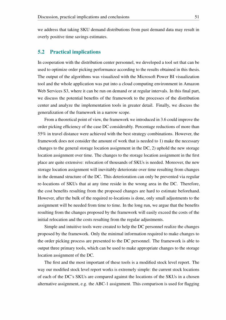
Discussion, practical implications and conclusions 51
we address that taking SKU demand distributions from past demand data may result in
overly positive time savings estimates.
5.2 Practical implications
In cooperation with the distribution center personnel, we developed a tool set that can be
used to optimize order picking performance according to the results obtained in this thesis.
The output of the algorithms was visualized with the Microsoft Power BI visualization
tool and the whole application was put into a cloud computing environment in Amazon
Web Services S3, where it can be run on demand or at regular intervals. In this final part,
we discuss the potential benefits of the framework to the processes of the distribution
center and analyze the implementation tools in greater detail. Finally, we discuss the
generalization of the framework in a narrow scope.
From a theoretical point of view, the framework we introduced in 3.6 could improve the
order picking efficiency of the case DC considerably. Percentage reductions of more than
55% in travel distance were achieved with the best strategy combinations. However, the
framework does not consider the amount of work that is needed to 1) make the necessary
changes to the general storage location assignment in the DC, 2) uphold the new storage
location assignment over time. The changes to the storage location assignment in the first
place are quite extensive: relocation of thousands of SKUs is needed. Moreover, the new
storage location assignment will inevitably deteriorate over time resulting from changes
in the demand structure of the DC. This deterioration can only be prevented via regular
re-locations of SKUs that at any time reside in the wrong area in the DC. Therefore,
the cost benefits resulting from the proposed changes are hard to estimate beforehand.
However, after the bulk of the required re-locations is done, only small adjustments to the
assignment will be needed from time to time. In the long run, we argue that the benefits
resulting from the changes proposed by the framework will easily exceed the costs of the
initial relocation and the costs resulting from the regular adjustments.
Simple and intuitive tools were created to help the DC personnel realize the changes
proposed by the framework. Only the minimal information required to make changes to
the order picking process are presented to the DC personnel. The framework is able to
output three primary tools, which can be used to make appropriate changes to the storage
location assignment of the DC.
The first and the most important of these tools is a modified stock level report. The
way our modified stock level report works is extremely simple: the current stock locations
of each of the DC’s SKUs are compared against the locations of the SKUs in a chosen
alternative assignment, e.g. the ABC-1 assignment. This comparison is used for flagging

Discussion, practical implications and conclusions 52
any SKU that has a stock place in the wrong turnover zone. Then, the warehouse personnel
may decide whether to move the SKU to the correct zone or let it stay where it is, depending
on the demand frequency of the SKU. The demand information is printed for each SKU
alongside the correct turnover class because the classes may contain items of differing
turnover rates. Within any zone, the warehouse personnel are free to choose the new stock
places as the assignments within the class should be random.
The second tool is used to run the cluster analysis of the SKUs and print the clusters
such that the warehouse personnel may decide the correct placement for the cluster based
on the number of unique SKUs in the cluster and the types of the items in the cluster. The
third tool is another modified stock level report: it contains information only on the SKUs
that are considered as having zero turnover rate based on the demand data. Due to the DC’s
high utilization rate, such items may needlessly occupy space in areas reserved for SKUs
belonging to the fast or intermediate class. This third tool was created for the sole purpose
of finding non-moving SKUs for relocation to the slow zone and for creating space in the
fast and intermediate zones for their respective SKUs. The third tool is important in the
initial phase of the SKU relocation as rack space must be freed from the fast item zones.
Time series of the DC’s order picking efficiency may be printed each time the model
is run via an optional parameter. The time series can be used by the DC personnel both
as a tool to monitor the current efficiency of the order picking process compared to a
simulated scenario as well as a diagnostic tool to assess the performance implications of
changes made to the storage location assignment. The time series will show the effects of
re-locations on the general efficiency level with a slight delay. In the long run, the time
series has an essential role in keeping the storage location assignment up to date with
changing demand patterns: deterioration of the storage location assignment can be directly
observed from an upward trend in the series. If such trends emerge, the model may be run
again to track and find the cause of them from the output lists, after which the required
changes to the storage location assignment can be made.
In addition to the three tools and the time series graph, the visualization tool is able to
output a chart that reports the current situation of the storage location assignment adhering
to a selected assignment for quick visual inspection. The chart reports the situations for
all six zones in the DC (see 3.2.1). An example chart can be found in appendix D. This
chart immediately shows to what degree the current storage location assignment follows
the selected assignment in each of the six zones.
The implementation of the framework written in the Python programming language is
located in a cloud-computing environment, the AWS (Amazon Web Services). Generation
of new tools to support the order picking process is automated: the end user need only set

Discussion, practical implications and conclusions 53
the requested parameters and the respective tools will be provided. The algorithms may be
run and the Power BI report generated on-demand.
Generalization of our framework to other distribution centers should be fairly straight-
forward as long as the underlying data structures remain unchanged. The most difficult
part about this would be the need to rewrite the picker routing algorithms for differently
shaped layouts.
5.3 Conclusions
The research question of this study was: "what is the most robust and optimal way to
arrange the order picking process of the manually operated case distribution center to
minimize order picking distance, and what are the main drivers behind improved order
picking performance?" Using class-based storage location assignments supplemented with
a correlation-based assignment and a simple order batching procedure, we showed that the
order picking distance could be reduced significantly. Our simulations show that travel
distance savings up to 55% compared to the DC’s current order picking process could
be achieved with relatively simple changes to the process. We observed, that in the case
distribution center, the main driver for better order picking performance was the storage
location assignment before order batching. This is mostly due to the distribution center
being very long and having few aisles. Moreover, we argue that due to this same reason, the
picker routing problem is the least important driver behind better order picking performance
in the case DC. We argue that using order batching, significant savings can be achieved
with very simple methods.
To come to this conclusion, we created a framework that analyzes and optimizes the
order picking process of a distribution center via simulations based on the historical SKU
demand patters of the DC. We employed a heuristic picker routing policy to calculate the
distance a picker must travel on the warehouse floor over a set of pick lists for a large set
of different SLAP and batching strategies. Furthermore, we deployed a solution based on
the framework into a cloud-computing environment, where the DC personnel may run the
program on-demand and visually inspect the condition of their order picking process.
The results obtained from the framework were mostly in line with existing literature.
Although there is a massive body of literature covering the order picking process in
a manual picker-to-parts warehouse, few papers even try to model the whole process.
Furthermore, few papers had created assignments using SKU clusters. Our research
was an experiment of doing this with an unorthodox warehouse layout. In spite of the
characteristics of the case warehouse, the underlying modeling process used in this paper
could easily be expanded or modified to accommodate different warehouses.

Discussion, practical implications and conclusions 54
This study contributed to the order picking literature in that it introduced a framework
that may easily be applied to real-world order picking processes in an end-to-end pipeline
taking into account the most critical issues in manual order picking.

References 55
References
Ankerst, M. et al. (1999). “OPTICS: Ordering Points to Identify the Clustering Structure”.
In: Proceedings of the ACM SIGMOID Conference, pp. 49–60.
Bartholdi, J. J. and S. T. Hackman (2011). Warehouse & Distribution Science. URL:
http://www.scl.gatech.edu/sites/default/files/downloads/gtscl-
warehouse_science_bartholdi.pdf.
Bindi, F. et al. (2009). “Similarity-based Storage Allocation Rules in an Order Picking
System: An Application to the Food Service Industry”. In: International Journal of
Logistics: Research and Applications 12.4, pp. 233–247.
Brynzer, H. and M. I. Johansson (2009). “Storage Location Assignment: Using the Product
Structure to Reduce Order Picking Times”. In: International Journal of Production
Economics 46-47, pp. 595–603.
Caron, F., G. Marchet, and A. Perego (1998). “Routing Policies and COI-based Storage
Policies in Picker-to-part Systems”. In: International Journal of Production Research
36.3, pp. 713–732.
Chen, C. -M. et al. (2009). “A Flexible Evaluative Framework for Order Picking Systems”.
In: Production and Operations Management 19.1, pp. 70–82.
Choe, K. and G. P. Sharp (1991). “Small Parts Order Picking: Design and Operation”. In:
Production and Operations Management. URL: https://www2.isye.gatech.edu/
~mgoetsch/cali/Logistics%20Tutorial/order/article.htm.
De Koster, R., T. Le-Duc, and K. J. Roodbergen (2007). “Design and Control of Warehouse
Order Picking: A Literature Review”. In: European Journal of Operational Research
182, pp. 481–501.
De Koster, R., E. S. Van Der Poort, and M. Wolters (1999). “Efficient orderbatching
methods in warehouses”. In: International Journal of Production Research 37.7,
pp. 1479–1504.
Dekker, R. et al. (2004). “Improving Order-Picking Response Time at Ankor’s Warehouse”.
In: Interfaces 34.4, pp. 303–313.
Le-Duc, T. (2005). “Design and Control of Efficient Order Picking Processes”. PhD thesis.
Erasmus University Rotterdam.
Le-Duc, T. and R. De Koster (2005). “Travel Distance Estimation and Storage Zone
Optimization in a 2-block Class-based Storage Strategy Warehouse”. In: International
Journal of Production Research 43.17, pp. 3561–3581.
References 56
Elsayed, E. A. (1981). “Algorithms for Optimal Material Handling in Automatic Ware-
housing Systems”. In: International Journal of Production Research 19.5, pp. 525–
535.
Gademann, N. and S. Van De Velde (2005). “Order Batching to Minimize Total Travel
Time in a Parallel-aisle Warehouse”. In: IIE Transactions 37, pp. 63–75.
Henn, S., S. Koch, et al. (2010). “Metaheuristics for the Order Batching Problem in
Manual Order Picking Systems”. In: Business Research 3.1, pp. 82–105.
Henn, S. and G. Wäscher (2012). “Tabu Search Heuristics for the Order Batching Problem
in Manual Order Picking Systems”. In: European Journal of Operational Research
222.3, pp. 484–494.
Hsieh, L. -F., C. -J. Huang, and C- .L. Huang (2007). “Applying Particle Swarm Optimiza-
tion to Schedule Order Picking Routes in a Distribution Center”. In: Asian Journal of
Management and Humanity Sciences 1.4, pp. 558–576.
Kallina, K. and J. Lynn (1976). “Application of the Cube-per-order Index Rule for Stock
Location in a Distribution Warehouse”. In: Interfaces 7.1, pp. 37–46.
Kofler, M. et al. (2015). “Robust Storage Assignment in Warehouses with Correlated
Demand”. In: Computational Intelligence and Efficiency in Engineering Systems 595,
pp. 415–428.
Liu, C. -M. (1999). “Clustering Techniques for Stock Location and Order-picking in a
Distribution Center”. In: Computers & Operations Research 26, pp. 989–1002.
Ma, T. and P. Zhao (2014). “A Review of Algorithms for Order Batching Problem in Dis-
tribution Center”. In: International Conference on Logistics Engineering Management
and Computer Science (LEMCS 2014).
Malmborg, C. J. and K. Bhaskaran (1990). “A Revised Proof of Optimality for the Cube-
per-order Index Rule for Stored Item Location”. In: Applied Mathematical Modelling
14, pp. 87–95.
Manzini, R. et al. (2007). “Similarity Coefficients and Clustering Techniques for the
Correlated Assignment Problem in Warehousing Systems”. In:
Pan, J. C. -H., P. -H. Shih, and M. -H. Wu (2015). “Order Batching in a Pick-and-pass
Warehousing System with Group Genetic Algorithm”. In: Omega 57 (Part B), pp. 238–
248.
Petersen, C. G. (1999). “The Impact of Routing and Storage Policies on Warehouse
Efficiency”. In: International Journal of Operations & Production Management 19.10,
pp. 1053–1064.
References 57
Petersen, C. G. and G. Aase (2004). “A Comparison of Picking, Storage, and Routing
Policies in Manual Order Picking”. In: International Journal of Production Economics
92, pp. 11–19.
— (2017). “Improving Order Picking Efficiency with the Use of Cross Aisles and Storage
Policies”. In: Open Journal of Business and Management 5.1, pp. 95–104.
Petersen, C. G., G. R. Aase, and D. R. Heiser (2004). “Improving Order Picking Perfor-
mance through the Implementation of Class-based Storage”. In: International Journal
of Physical Distribution & Logistics Management 34.7, pp. 534–544.
Petersen, C. G. and R. W. Schmenner (1999). “An Evaluation of Routing and Volume-
based Storage Policies in an Order Picking Operation”. In: Decision Sciences 30.2,
pp. 481–501.
Pohl, L. M., R. D. Meller, and K. R. Gue (2011). “Turnover-based Storage in Non-
traditional Unit-load Warehouse Designs”. In: IIE Transactions 43, pp. 703–720.
Ratliff, H. D. and A. Rosenthal (1983). “Order-Picking in a Rectangular Warehouse: A
Solvable Case of the Traveling Salesman Problem”. In: Operations Research 31.3,
pp. 507–521.
Roodbergen, K. J. and R. De Koster (2001a). “Routing Methods for Warehouses with Mul-
tiple Cross Aisles”. In: International Journal of Production Research 39.9, pp. 1865–
1883.
— (2001b). “Routing Order Pickers in a Warehouse with a Middle Aisle”. In: European
Journal of Operational Research 133.1, pp. 32–43.
Schwarz, L. B., S. C. Graves, and W. H. Hausman (1978). “Scheduling Policies for
Automatic Warehousing Systems: Simulation Results”. In: A I I E Transactions 10.3,
pp. 260–270.
Won, J. and S. Olafsson (2005). “Joint Order Batching and Order Picking in Warehouse
Operations”. In: International Journal of Production Research 43.7, pp. 1427–1442.
Zhang, R. -Q., M. Wang, and X. Pan (2019). “New Model of the Storage Location
Assignment Problem Considering Demand Correlation Pattern”. In: Computers &
Industrial Engineering 129, pp. 210–2019.
Zhang, Y. (2016). “Correlated Storage Assignment Strategy to Reduce Travel Distance in
Order Picking”. In: IFAC-PapersOnLine 49.2, pp. 30–35.
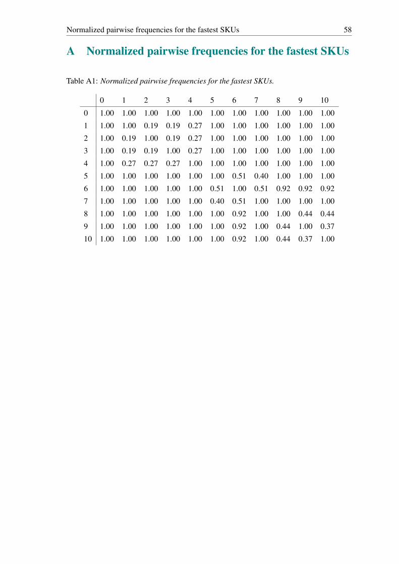
Normalized pairwise frequencies for the fastest SKUs 58
A Normalized pairwise frequencies for the fastest SKUs
Table A1: Normalized pairwise frequencies for the fastest SKUs.
0 1 2 3 4 5 6 7 8 9 10
0 1.00 1.00 1.00 1.00 1.00 1.00 1.00 1.00 1.00 1.00 1.00
1 1.00 1.00 0.19 0.19 0.27 1.00 1.00 1.00 1.00 1.00 1.00
2 1.00 0.19 1.00 0.19 0.27 1.00 1.00 1.00 1.00 1.00 1.00
3 1.00 0.19 0.19 1.00 0.27 1.00 1.00 1.00 1.00 1.00 1.00
4 1.00 0.27 0.27 0.27 1.00 1.00 1.00 1.00 1.00 1.00 1.00
5 1.00 1.00 1.00 1.00 1.00 1.00 0.51 0.40 1.00 1.00 1.00
6 1.00 1.00 1.00 1.00 1.00 0.51 1.00 0.51 0.92 0.92 0.92
7 1.00 1.00 1.00 1.00 1.00 0.40 0.51 1.00 1.00 1.00 1.00
8 1.00 1.00 1.00 1.00 1.00 1.00 0.92 1.00 1.00 0.44 0.44
9 1.00 1.00 1.00 1.00 1.00 1.00 0.92 1.00 0.44 1.00 0.37
10 1.00 1.00 1.00 1.00 1.00 1.00 0.92 1.00 0.44 0.37 1.00
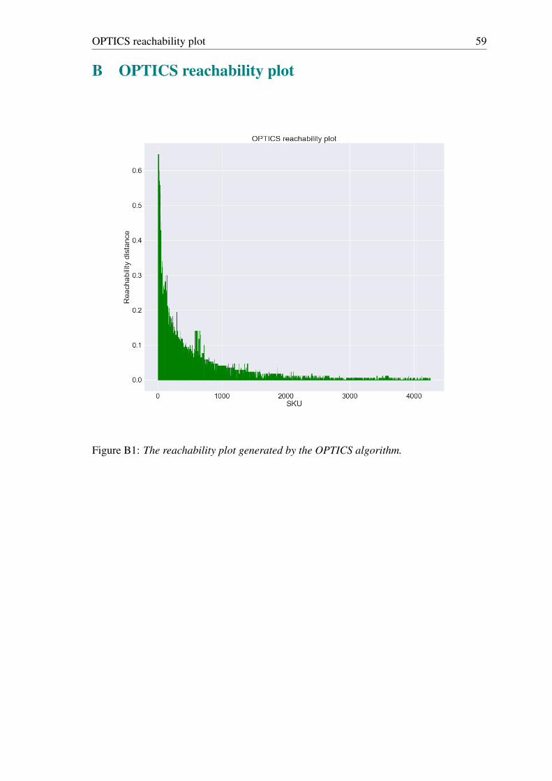
OPTICS reachability plot 59
B OPTICS reachability plot
Figure B1: The reachability plot generated by the OPTICS algorithm.
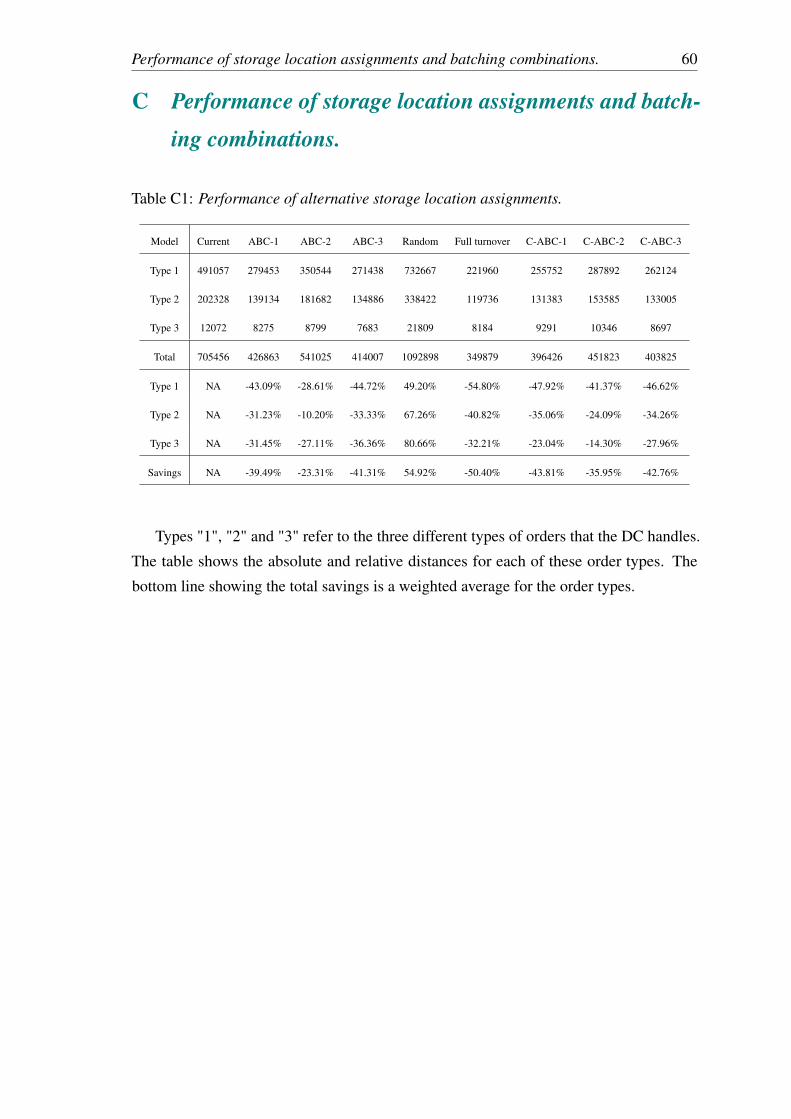
Performance of storage location assignments and batching combinations. 60
C Performance of storage location assignments and batch-
ing combinations.
Table C1: Performance of alternative storage location assignments.
Model Current ABC-1 ABC-2 ABC-3 Random Full turnover C-ABC-1 C-ABC-2 C-ABC-3
Type 1 491057 279453 350544 271438 732667 221960 255752 287892 262124
Type 2 202328 139134 181682 134886 338422 119736 131383 153585 133005
Type 3 12072 8275 8799 7683 21809 8184 9291 10346 8697
Total 705456 426863 541025 414007 1092898 349879 396426 451823 403825
Type 1 NA -43.09% -28.61% -44.72% 49.20% -54.80% -47.92% -41.37% -46.62%
Type 2 NA -31.23% -10.20% -33.33% 67.26% -40.82% -35.06% -24.09% -34.26%
Type 3 NA -31.45% -27.11% -36.36% 80.66% -32.21% -23.04% -14.30% -27.96%
Savings NA -39.49% -23.31% -41.31% 54.92% -50.40% -43.81% -35.95% -42.76%
Types "1", "2" and "3" refer to the three different types of orders that the DC handles.
The table shows the absolute and relative distances for each of these order types. The
bottom line showing the total savings is a weighted average for the order types.

Performance of storage location assignments and batching combinations. 61
Table C2: Performance of all batching and storage location assignment combinations.
Current ABC-1 ABC-2 ABC-3 Random Full turnover C-ABC-1 C-ABC-2 C-ABC-3
FCFS 705456 426863 541025 414007 1092898 349879 396426 451823 403825
Seed algorithm 540469 323781 395425 313529 766049 236846 299871 341195 301576
Compared to
FCFS
-23.39% -24.15% -26.91% -24.27% -29.91% -32.31% -24.36% -24.48% -25.32%
Random algo-
rithm
565927 353977 420249 340184 834693 273355 328488 366305 329041
Compared to
FCFS
-19.78% -17.07% -22.32% -17.83% -23.63% -21.87% -17.14% -18.93% -18.52%
Total savings
(Compared to
current FCFS)
Seed algorithm -23.39% -54.10% -43.95% -55.56% 8.59% -66.43% -57.49% -51.63% -57.25%
Random algo-
rithm
-19.78% -49.82% -40.43% -51.78% 18.32% -61.25% -53.44% -48.08% -53.36%
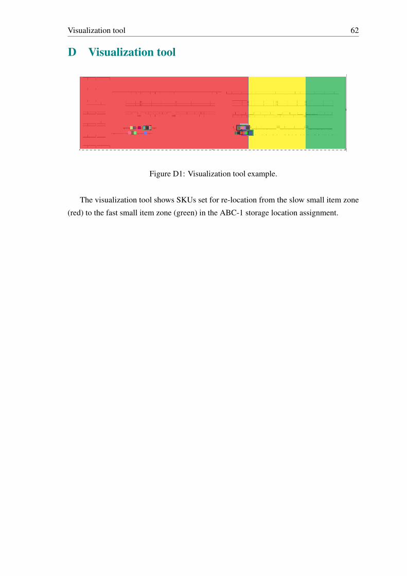
Visualization tool 62
D Visualization tool
Figure D1: Visualization tool example.
The visualization tool shows SKUs set for re-location from the slow small item zone
(red) to the fast small item zone (green) in the ABC-1 storage location assignment.