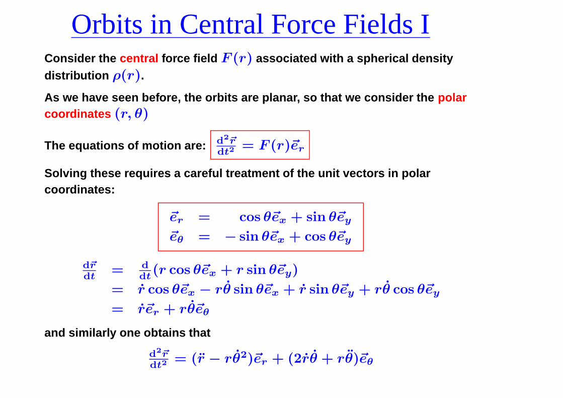
Orbits in Central Force Fields IConsider the central force field F (r) associated with a spherical densitydistribution ρ(r).

As we have seen before, the orbits are planar, so that we consider the polarcoordinates (r, θ)

The equations of motion are: d2~rdt2

= F (r)~er

Solving these requires a careful treatment of the unit vectors in polarcoordinates:

~er = − cos θ~ex + sin θ~ey

~eθ = − sin θ~ex + cos θ~ey

d~rdt

= ddt

(r cos θ~ex + r sin θ~ey)

= r cos θ~ex − rθ sin θ~ex + r sin θ~ey + rθ cos θ~ey

= r~er + rθ~eθ

and similarly one obtains that

d2~rdt2

= (r − rθ2)~er + (2rθ + rθ)~eθ

Orbits in Central Force Fields IIWe thus obtain the following set of equations of motions:

r − rθ2 = F (r) = −dΦdr

2rθ + rθ = 0

Multiplying the second of these equations with r yields, after integration, thatddt

(r2θ) = 0. This simply expresses the conservation of the orbit’s angular

momentum L = r2θ, i.e., the equations of motion can be written as

r − rθ2 = −dΦdr

r2θ = L = constant

In general these equations have to be solved numerically. Despite the verysimple, highly symmetric system, the equations of motion don’t providemuch insight. As we’ll see later, more direct insight is obtained by focussingon the conserved quantities. Note also that the equations of motion aredifferent in different coordinate systems: in Cartesian coordinates (x, y):

x = Fx = −∂Φ∂x

y = Fy = −∂Φ∂y

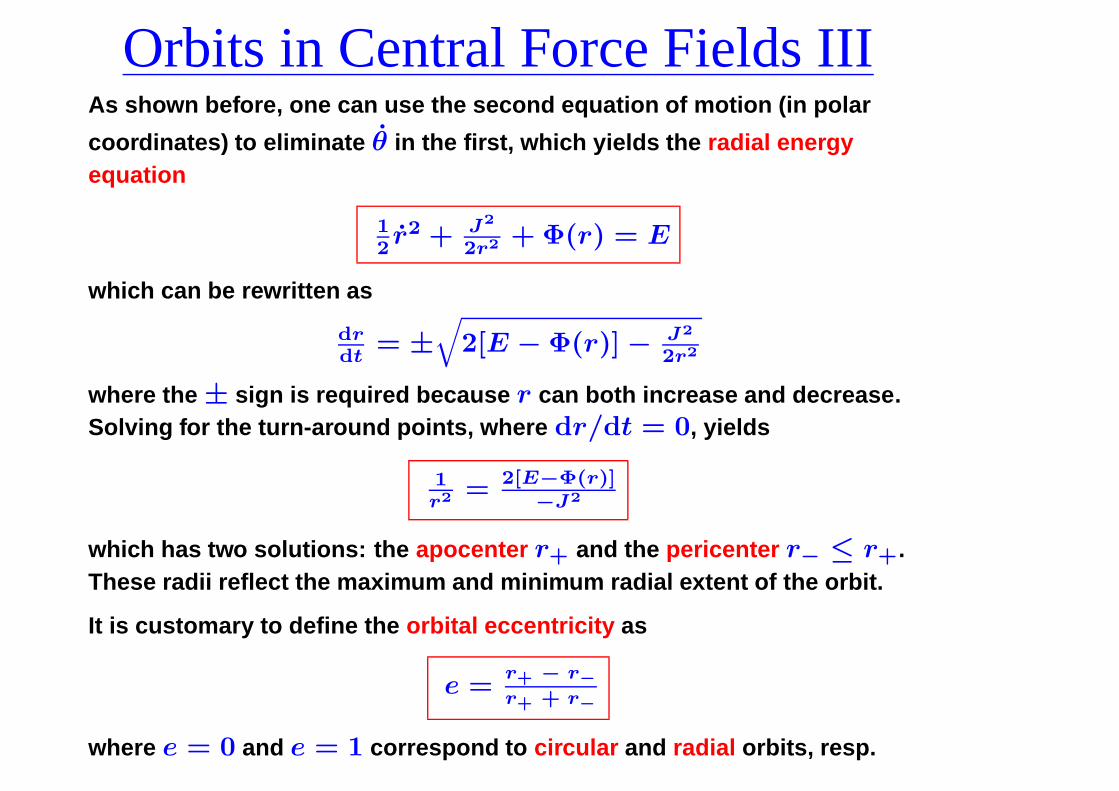
Orbits in Central Force Fields IIIAs shown before, one can use the second equation of motion (in polar

coordinates) to eliminate θ in the first, which yields the radial energyequation

12r2 + J2

2r2 + Φ(r) = E

which can be rewritten as

drdt

= ±√

2[E − Φ(r)] − J2

2r2

where the ± sign is required because r can both increase and decrease.Solving for the turn-around points, where dr/dt = 0, yields

1r2 = 2[E−Φ(r)]

−J2

which has two solutions: the apocenter r+ and the pericenter r− ≤ r+.These radii reflect the maximum and minimum radial extent of the orbit.

It is customary to define the orbital eccentricity as

e =r+ − r−

r+ + r−

where e = 0 and e = 1 correspond to circular and radial orbits, resp.

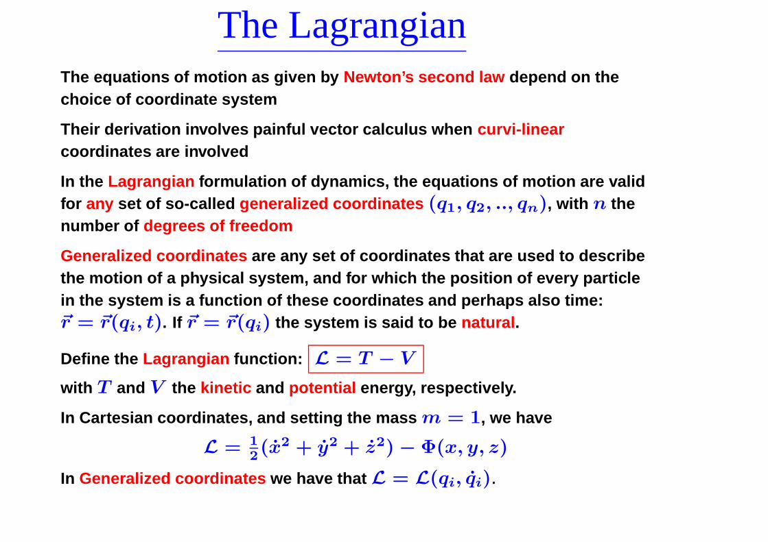
The LagrangianThe equations of motion as given by Newton’s second law depend on thechoice of coordinate system

Their derivation involves painful vector calculus when curvi-linearcoordinates are involved

In the Lagrangian formulation of dynamics, the equations of motion are validfor any set of so-called generalized coordinates (q1, q2, .., qn), with n thenumber of degrees of freedom

Generalized coordinates are any set of coordinates that are used to describethe motion of a physical system, and for which the position of every particlein the system is a function of these coordinates and perhaps also time:~r = ~r(qi, t). If ~r = ~r(qi) the system is said to be natural.

Define the Lagrangian function: L = T − V

with T and V the kinetic and potential energy, respectively.

In Cartesian coordinates, and setting the mass m = 1, we have

L = 12(x2 + y2 + z2) − Φ(x, y, z)

In Generalized coordinates we have that L = L(qi, qi).

Actions and Hamilton’s Principle

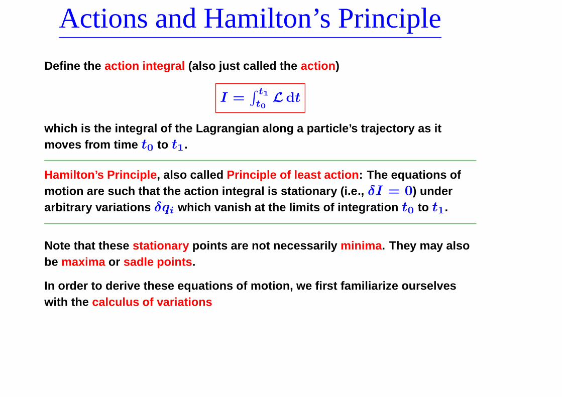
Define the action integral (also just called the action)

I =∫ t1

t0L dt

which is the integral of the Lagrangian along a particle’s trajectory as itmoves from time t0 to t1.

Hamilton’s Principle, also called Principle of least action: The equations ofmotion are such that the action integral is stationary (i.e., δI = 0) underarbitrary variations δqi which vanish at the limits of integration t0 to t1.

Note that these stationary points are not necessarily minima. They may alsobe maxima or sadle points.

In order to derive these equations of motion, we first familiarize ourselveswith the calculus of variations

Calculus of Variations IWe are interested in finding the stationary values of an integral of the form

I =x1∫

x0

f(y, y)dx

where f(y, y) is a specified function of y = y(x) and y = dy/dx.

x(0)

x(1)y

x

y(x)δy

Consider a small variation δy(x), which vanishes at the endpoints of theintegration interval: δy(x0) = δy(x1) = 0

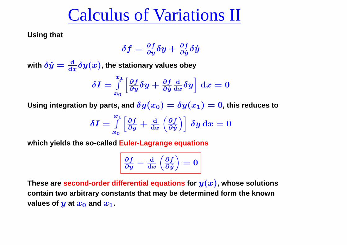
Calculus of Variations IIUsing that

δf = ∂f

∂yδy + ∂f

∂yδy

with δy = ddx

δy(x), the stationary values obey

δI =x1∫

x0

[

∂f

∂yδy + ∂f

∂yddx

δy]

dx = 0

Using integration by parts, and δy(x0) = δy(x1) = 0, this reduces to

δI =x1∫

x0

[

∂f

∂y+ d

dx

(

∂f

∂y

)]

δy dx = 0

which yields the so-called Euler-Lagrange equations

∂f

∂y− d

dx

(

∂f

∂y

)

= 0

These are second-order differential equations for y(x), whose solutionscontain two arbitrary constants that may be determined form the knownvalues of y at x0 and x1.

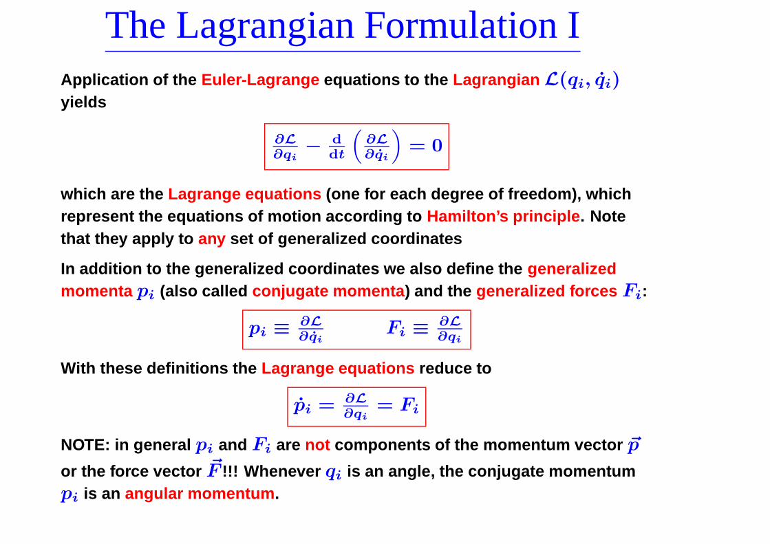
The Lagrangian Formulation IApplication of the Euler-Lagrange equations to the Lagrangian L(qi, qi)yields

∂L

∂qi− d

dt

(

∂L

∂qi

)

= 0

which are the Lagrange equations (one for each degree of freedom), whichrepresent the equations of motion according to Hamilton’s principle. Notethat they apply to any set of generalized coordinates

In addition to the generalized coordinates we also define the generalizedmomenta pi (also called conjugate momenta) and the generalized forces Fi:

pi ≡ ∂L

∂qiFi ≡ ∂L

∂qi

With these definitions the Lagrange equations reduce to

pi = ∂L

∂qi= Fi

NOTE: in general pi and Fi are not components of the momentum vector ~p

or the force vector ~F !!! Whenever qi is an angle, the conjugate momentumpi is an angular momentum.

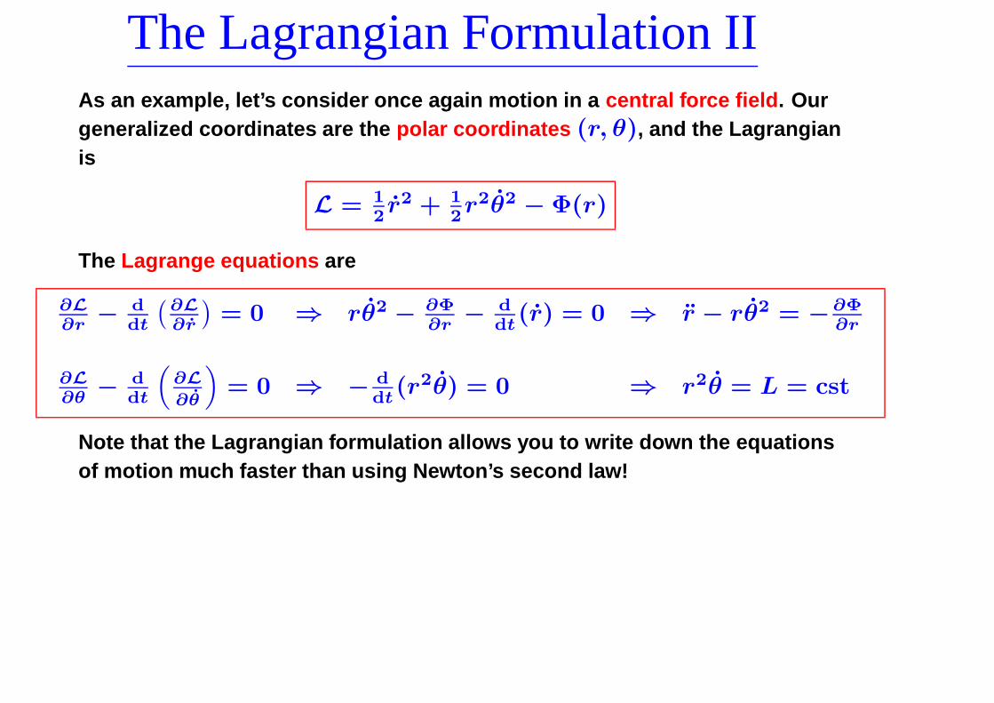
The Lagrangian Formulation IIAs an example, let’s consider once again motion in a central force field. Ourgeneralized coordinates are the polar coordinates (r, θ), and the Lagrangianis

L = 12r2 + 1

2r2θ2 − Φ(r)

The Lagrange equations are

∂L

∂r− d

dt

(

∂L

∂r

)

= 0 ⇒ rθ2 − ∂Φ∂r

− ddt

(r) = 0 ⇒ r − rθ2 = −∂Φ∂r

∂L

∂θ− d

dt

(

∂L

∂θ

)

= 0 ⇒ − ddt

(r2θ) = 0 ⇒ r2θ = L = cst

Note that the Lagrangian formulation allows you to write down the equationsof motion much faster than using Newton’s second law!

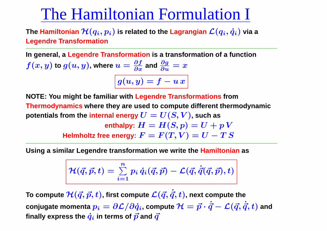
The Hamiltonian Formulation IThe Hamiltonian H(qi, pi) is related to the Lagrangian L(qi, qi) via aLegendre Transformation

In general, a Legendre Transformation is a transformation of a function

f(x, y) to g(u, y), where u = ∂f

∂xand ∂g

∂u= x

g(u, y) = f − u x

NOTE: You might be familiar with Legendre Transformations fromThermodynamics where they are used to compute different thermodynamicpotentials from the internal energy U = U(S, V ), such as

enthalpy: H = H(S, p) = U + p V

Helmholtz free energy: F = F (T, V ) = U − T S

Using a similar Legendre transformation we write the Hamiltonian as

H(~q, ~p, t) =n∑

i=1

pi qi(~q, ~p) − L(~q, ~q(~q, ~p), t)

To compute H(~q, ~p, t), first compute L(~q, ~q, t), next compute the

conjugate momenta pi = ∂L/∂qi, compute H = ~p · ~q − L(~q, ~q, t) andfinally express the qi in terms of ~p and ~q

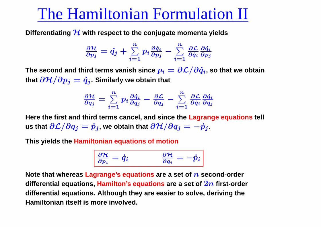
The Hamiltonian Formulation IIDifferentiating H with respect to the conjugate momenta yields

∂H

∂pj= qj +

n∑

i=1

pi∂qi

∂pj−

n∑

i=1

∂L

∂qi

∂qi

∂pj

The second and third terms vanish since pi = ∂L/∂qi, so that we obtainthat ∂H/∂pj = qj . Similarly we obtain that

∂H

∂qj=

n∑

i=1

pi∂qi

∂qj− ∂L

∂qj−

n∑

i=1

∂L

∂qi

∂qi

∂qj

Here the first and third terms cancel, and since the Lagrange equations tellus that ∂L/∂qj = pj , we obtain that ∂H/∂qj = −pj .

This yields the Hamiltonian equations of motion

∂H

∂pi= qi

∂H

∂qi= −pi

Note that whereas Lagrange’s equations are a set of n second-orderdifferential equations, Hamilton’s equations are a set of 2n first-orderdifferential equations. Although they are easier to solve, deriving theHamiltonian itself is more involved.

The Hamiltonian Formulation IIIThe Hamiltonian description is especially useful for finding conservedquantities, which will play an important role in describing orbits.

If a generalized coordinate, say qi, does not appear in the Hamiltonian, thenthe corresponding conjugate momentum pi is a conserved quantity!!!

In the case of motion in a fixed potential, the Hamiltonian is equal to the totalenergy, i.e., H = E

DEMONSTRATION: for a time-independent potential Φ = Φ(~x) the

Lagrangian is equal to L = 12~x2 − Φ(~x). Since ~p = ∂L/∂~x = ~x we

have that H = ~x · ~x − 12~x2 + Φ(~x) = 1

2~x2 + Φ(~x) = E

The 2n-dimensional phase-space of a dynamical system with n degrees offreedom can be described by the generalized coordinates and momenta(~q, ~p). Since Hamilton’s equations are first order differential equations, wecan determine ~q(t) and ~p(t) at any time t once the initial conditions(~q0, ~p0) are given. Therefore, through each point in phase-space therepasses a unique trajectory Γ[~q(~q0, ~p0, t), ~p(~q0, ~p0, t)]. No two trajectoriesΓ1 and Γ2 can pass through the same (~q0, ~p0) unless Γ1 = Γ2.

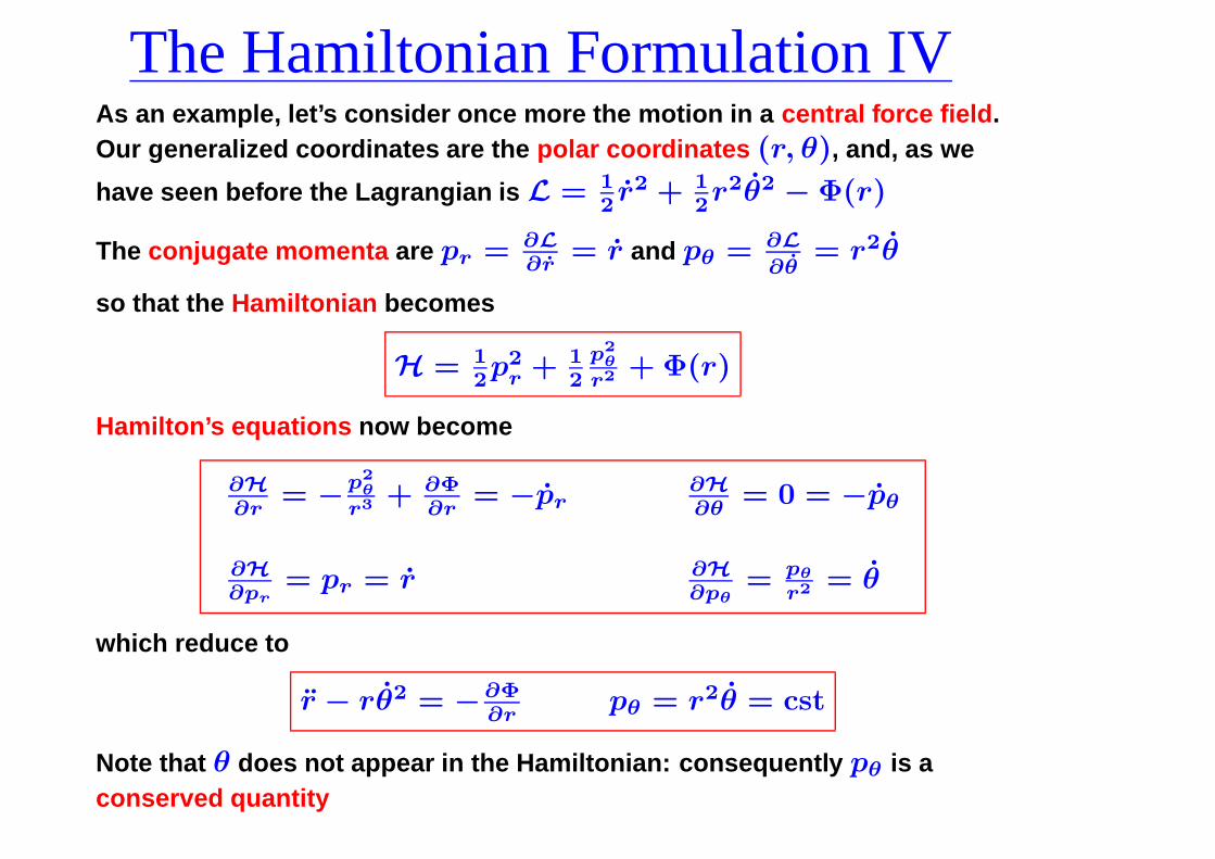
The Hamiltonian Formulation IVAs an example, let’s consider once more the motion in a central force field.Our generalized coordinates are the polar coordinates (r, θ), and, as we

have seen before the Lagrangian is L = 12r2 + 1

2r2θ2 − Φ(r)

The conjugate momenta are pr = ∂L

∂r= r and pθ = ∂L

∂θ= r2θ

so that the Hamiltonian becomes

H = 12p2

r + 12

p2θ

r2 + Φ(r)

Hamilton’s equations now become

∂H

∂r= −

p2θ

r3 + ∂Φ∂r

= −pr∂H

∂θ= 0 = −pθ

∂H

∂pr= pr = r ∂H

∂pθ= pθ

r2 = θ

which reduce to

r − rθ2 = −∂Φ∂r

pθ = r2θ = cst

Note that θ does not appear in the Hamiltonian: consequently pθ is aconserved quantity

Noether’s TheoremIn 1915 the German mathematician Emmy Noether proved an importanttheorem which plays a trully central role in theoretical physics.

Noether’s Theorem: If an ordinary Lagrangian posseses some continuous,smooth symmetry, then there will be a conservationlaw associated with that symmetry.

• Invariance of L under time translation → energy conservation

• Invariance of L under spatial translation → momentum conservation

• Invariance of L under rotational translation → ang. mom. conservation

• Gauge Invariance of electric potential → charge conservation

Some of these symmetries are immediately evident from the Lagrangian:

• If L does not explicitely depend on t then E is conserved

• If L does not explicitely depend on qi then pi is conserved

Poisson Brackets IDEFINITION: Let A(~q, ~p) and B(~q, ~p) be two functions of the generalizedcoordinates and their conjugate momenta, then the Poisson bracket of Aand B is defined by

[A, B] =n∑

i=1

[

∂A∂qi

∂B∂pi

− ∂A∂pi

∂B∂qi

]

Let f = f(~q, ~p, t) then

df = ∂f

∂qidqi + ∂f

∂pidpi + ∂f

∂tdt

where we have used the summation convention. This differential of f ,combined with Hamilton’s equations, allows us to write

df

dt= ∂f

∂t+ ∂f

∂qi

∂H

∂pi− ∂f

∂pi

∂H

∂qi

which reduces to

df

dt= ∂f

∂t+ [f, H]

This is often called Poisson’s equation of motion. It shows that thetime-evolution of any dynamical variable is governed by the Hamiltonianthrough the Poisson bracket of the variable with the Hamiltonian.

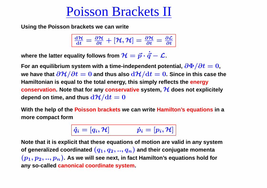
Poisson Brackets IIUsing the Poisson brackets we can write

dH

dt= ∂H

∂t+ [H, H] = ∂H

∂t= ∂L

∂t

where the latter equality follows from H = ~p · ~q − L.

For an equilibrium system with a time-independent potential, ∂Φ/∂t = 0,we have that ∂H/∂t = 0 and thus also dH/dt = 0. Since in this case theHamiltonian is equal to the total energy, this simply reflects the energyconservation. Note that for any conservative system, H does not explicitelydepend on time, and thus dH/dt = 0

With the help of the Poisson brackets we can write Hamilton’s equations in amore compact form

qi = [qi, H] pi = [pi, H]

Note that it is explicit that these equations of motion are valid in any systemof generalized coordinated (q1, q2, .., qn) and their conjugate momenta(p1, p2, .., pn). As we will see next, in fact Hamilton’s equations hold forany so-called canonical coordinate system.

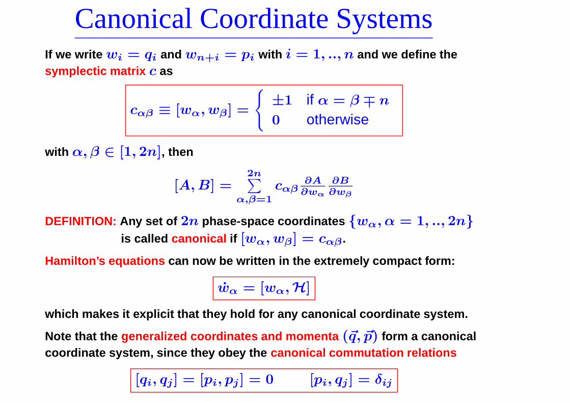
Canonical Coordinate SystemsIf we write wi = qi and wn+i = pi with i = 1, .., n and we define thesymplectic matrix c as

cαβ ≡ [wα, wβ] =

±1 if α = β ∓ n

0 otherwise

with α, β ∈ [1, 2n], then

[A, B] =2n∑

α,β=1

cαβ∂A

∂wα

∂B∂wβ

DEFINITION: Any set of 2n phase-space coordinates wα, α = 1, .., 2nis called canonical if [wα, wβ] = cαβ .

Hamilton’s equations can now be written in the extremely compact form:

wα = [wα, H]

which makes it explicit that they hold for any canonical coordinate system.

Note that the generalized coordinates and momenta (~q, ~p) form a canonicalcoordinate system, since they obey the canonical commutation relations

[qi, qj] = [pi, pj ] = 0 [pi, qj ] = δij

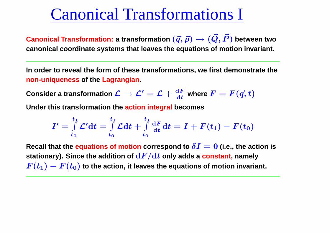
Canonical Transformations ICanonical Transformation: a transformation (~q, ~p) → (~Q, ~P ) between twocanonical coordinate systems that leaves the equations of motion invariant.

In order to reveal the form of these transformations, we first demonstrate thenon-uniqueness of the Lagrangian.

Consider a transformation L → L′ = L + dFdt

where F = F (~q, t)

Under this transformation the action integral becomes

I′ =t1∫

t0

L′dt =t1∫

t0

Ldt +t1∫

t0

dFdt

dt = I + F (t1) − F (t0)

Recall that the equations of motion correspond to δI = 0 (i.e., the action isstationary). Since the addition of dF/dt only adds a constant, namelyF (t1) − F (t0) to the action, it leaves the equations of motion invariant.

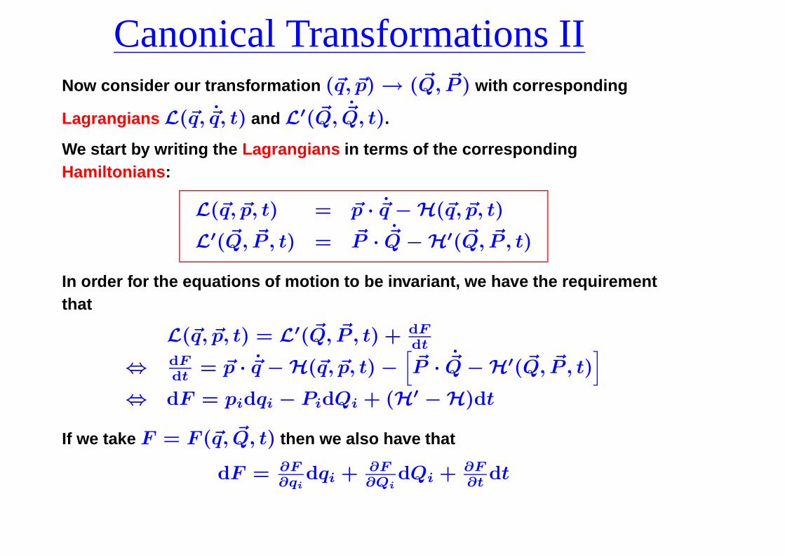
Canonical Transformations IINow consider our transformation (~q, ~p) → (~Q, ~P ) with corresponding

Lagrangians L(~q, ~q, t) and L′(~Q, ~Q, t).

We start by writing the Lagrangians in terms of the correspondingHamiltonians:

L(~q, ~p, t) = ~p · ~q − H(~q, ~p, t)

L′(~Q, ~P , t) = ~P · ~Q − H′(~Q, ~P , t)

In order for the equations of motion to be invariant, we have the requirementthat

L(~q, ~p, t) = L′(~Q, ~P , t) + dFdt

⇔ dFdt

= ~p · ~q − H(~q, ~p, t) −[

~P · ~Q − H′(~Q, ~P , t)]

⇔ dF = pidqi − PidQi + (H′ − H)dt

If we take F = F (~q, ~Q, t) then we also have that

dF = ∂F∂qi

dqi + ∂F∂Qi

dQi + ∂F∂t

dt

Canonical Transformations IIIEquating the two expressions for the differential dF yields thetransformation rules

pi = ∂F∂qi

Pi = − ∂F∂Qi

H′ = H + ∂F∂t

The function F (~q, ~Q, t) is called the generating function of the canonical

transformation (~q, ~p) → (~Q, ~P )

In order to transform (~q, ~p) → (~Q, ~P ) one proceeds as follows:

• Find a function F (~q, ~Q) so that pi = ∂F/∂qi. This yields Qi(qj, pj)

• Substitute Qi(qj , pj) in Pi = ∂F/∂Qi to obtain Pi(qj, pj)

As an example consider the generating function F (~q, ~Q) = qiOi.According to the transformation rules we have that

pi = ∂F∂qi

= Qi Pi = − ∂F∂Qi

= −qi

We thus have that Qi = pi and Pi = −qi: the canonical transformationhas changed the roles of coordinates and momenta, eventhough theequations of motion have remained invariant! This shows that there is nospecial status to either generalized coordinates or their conjugate momenta

Canonical Transformations IVFor reasons that will become clear later, in practice it is more useful to

consider a generating function of the form S = S(~q, ~P , t), i.e., one thatdepends on the old coordinates and the new momenta.

To derive the corresponding transformation rules, we start with the

generating function F = F (~q, ~Q, t), and recall that

dF = pidqi − PidQi + (H′ − H)dt

using that PidQi = d(QiPi) − QidPi, we obtain

d(F + QiPi) = pidqi + QidPi + (H′ − H)dt

Defining the new generator S(~q, ~Q, ~P , t) ≡ F (~q, ~Q, t) + ~Q · ~P , for which

dS = ∂S∂qi

dqi + ∂S∂Qi

dQi + ∂S∂Pi

dPi + ∂S∂t

dt

Equating this to the above we find the transformation rules

pi = ∂S∂qi

Qi = ∂S∂Pi

∂S∂Qi

= 0 H′ = H + ∂S∂t

Note that the third of these rules implies that S = S(~q, ~P , t) as intended.

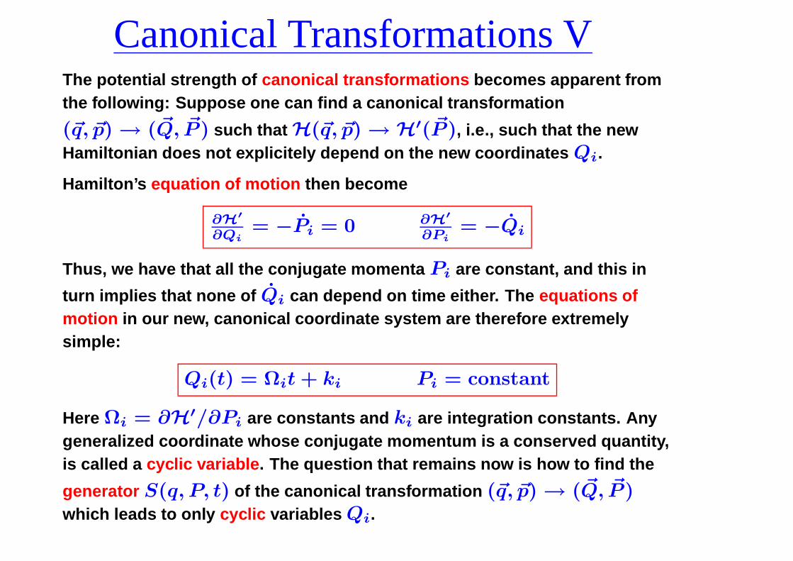
Canonical Transformations VThe potential strength of canonical transformations becomes apparent fromthe following: Suppose one can find a canonical transformation

(~q, ~p) → (~Q, ~P ) such that H(~q, ~p) → H′( ~P ), i.e., such that the newHamiltonian does not explicitely depend on the new coordinates Qi.

Hamilton’s equation of motion then become

∂H′

∂Qi= −Pi = 0 ∂H

′

∂Pi= −Qi

Thus, we have that all the conjugate momenta Pi are constant, and this in

turn implies that none of Qi can depend on time either. The equations ofmotion in our new, canonical coordinate system are therefore extremelysimple:

Qi(t) = Ωit + ki Pi = constant

Here Ωi = ∂H′/∂Pi are constants and ki are integration constants. Anygeneralized coordinate whose conjugate momentum is a conserved quantity,is called a cyclic variable. The question that remains now is how to find the

generator S(q, P, t) of the canonical transformation (~q, ~p) → (~Q, ~P )which leads to only cyclic variables Qi.

The Hamilton-Jacobi Equation IRecall the transformation rules for the generator S(~q, ~P , t):

pi = ∂S∂qi

Qi = ∂S∂Pi

H′ = H + ∂S∂t

If for simplicity we consider a generator that does not explicitely depend on

time, i.e., ∂S/∂t = 0 then we have that H(~q, ~p) = H′(~P ) = E. If wenow substitute ∂S/∂qi for pi in the original Hamiltonian we obtain

H(

∂S∂qi

, qi

)

= E

This is the Hamilton-Jacobi equation, which is a partial differential equation.

If it can be solved for S(~q, ~P ) than, as we have seen above, basically theentire dynamics are solved.

Thus, for a dynamical system with n degrees of freedom, one can solve thedynamics in one of the three following ways:

• Solve n second-order differential equations (Lagrangian formalism)

• Solve 2n first-order differential equations (Hamiltonian formalism)

• Solve a single partial differential equation (Hamilton-Jacobi equation)

The Hamilton-Jacobi Equation IIAlthough it may seem an attractive option to try and solve theHamilton-Jacobi equation, solving partial differential equations is in generalmuch more difficult than solving ordinary differential equations, and theHamilton-Jacobi equation is no exception.

However, in the specific case where the generator S is separable, i.e., if

S(~q, ~P ) =n∑

i=1

fi(qi)

with fi a set of n independent functions, then the Hamilton-Jacobi equationsplits in a set of n ordinary differential equations which are easily solved byquadrature. The integration constants are related to the (constant) conjugatemomenta Pi.

A Hamiltonian is called ‘integrable’ if the Hamilton-Jacobi equation is separable

Integrable Hamiltonians are extremely rare. Mathematically speaking theyform a set of measure zero in the space of all Hamiltonians. In what follows,we establish the link between so-called isolating integrals of motion andwhether or not a Hamiltonian is integrable.