orbital electronic systems - research collection
TRANSCRIPT

Research Collection
Doctoral Thesis
Effects of strong correlations on low-dimensional and multi-orbital electronic systems
Author(s): Indergand, Martin Franz
Publication Date: 2006
Permanent Link: https://doi.org/10.3929/ethz-a-005274292
Rights / License: In Copyright - Non-Commercial Use Permitted
This page was generated automatically upon download from the ETH Zurich Research Collection. For moreinformation please consult the Terms of use.
ETH Library

Diss. ETH No. 16864
Effects of strong correlations on
low-dimensional and multi-orbital
ELECTRONIC systems
A dissertation submitted to the
Swiss Federal Institute Of Technology Zurich
(ETH Zürich)
for the degree of
Doctor of Natural Sciences
presented by
Martin Indergand
Dipl. Phys. ETH
born February 21, 1975
Swiss citizen
accepted on the recommendation of
Prof. Dr. M. Sigrist, examiner
Prof. Dr. C. Honerkamp, co-examiner
Dr. A. Läuchli, co-examiner
2006

Seite Leer /
Blank leaf

Seite Leer /
Blank leaf

Seite Leer /
Blank leaf
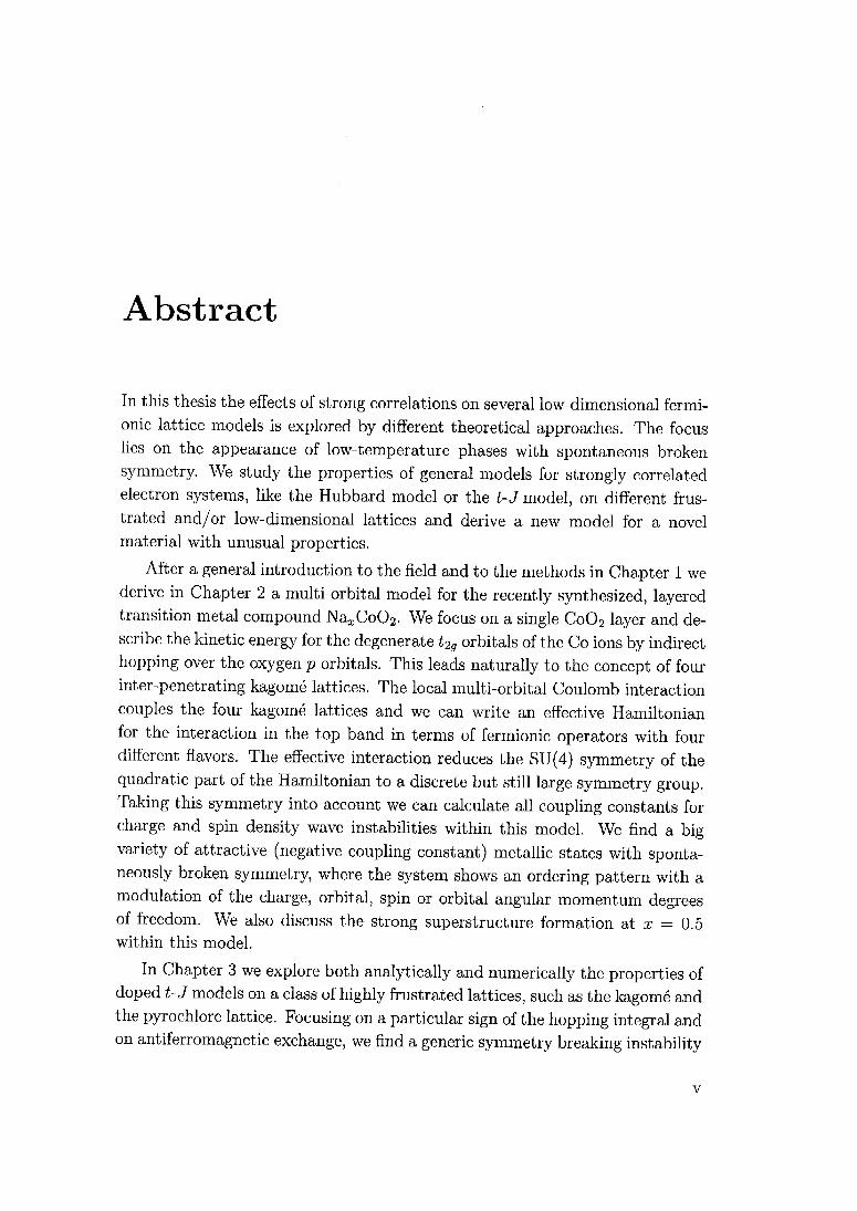
Abstract
In this thesis the effects of strong correlations on several low-dimensional fermi-
onic lattice models is explored by different theoretical approaches. The focus
lies on the appearance of low-temperature phases with spontaneous broken
symmetry. We study the properties of general models for strongly correlated
electron systems, like the Hubbard model or the t-J model, on different frus¬
trated and/or low-dimensional lattices and derive a new model for a novel
material with unusual properties.
After a general introduction to the field and to the methods in Chapter 1 we
derive in Chapter 2 a multi-orbital model for the recently synthesized, layeredtransition metal compound Na^CûC^- We focus on a single C0O2 layer and de¬
scribe the kinetic energy for the degenerate t^g orbitals of the Co ions by indirect
hopping over the oxygen p orbitals. This leads naturally to the concept of four
inter-penetrating kagomé lattices. The local multi-orbital Coulomb interaction
couples the four kagomé lattices and we can write an effective Hamiltonian
for the interaction in the top band in terms of fermionic operators with four
different flavors. The effective interaction reduces the SU(4) symmetry of the
quadratic part of the Hamiltonian to a discrete but still large symmetry group.
Taking this symmetry into account we can calculate all coupling constants for
charge and spin density wave instabilities within this model. We find a bigvariety of attractive (negative coupling constant) metallic states with sponta¬
neously broken symmetry, where the system shows an ordering pattern with a
modulation of the charge, orbital, spin or orbital angular momentum degreesof freedom. We also discuss the strong superstructure formation at x — 0.5
within this model.
In Chapter 3 we explore both analytically and numerically the properties of
doped t-J models on a class of highly frustrated lattices, such as the kagomé and
the pyrochlore lattice. Focusing on a particular sign of the hopping integral andon antiferromagnetic exchange, we find a generic symmetry breaking instability
v
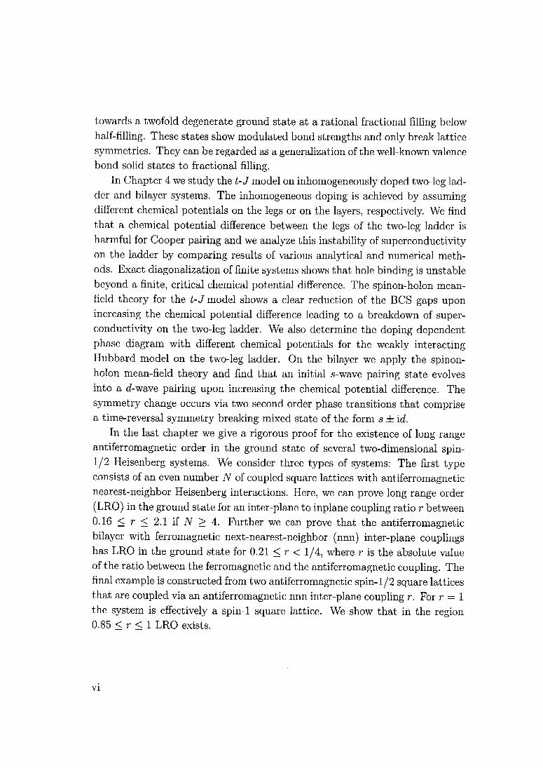
towards a twofold degenerate ground state at a rational fractional filling below
half-filling. These states show modulated bond strengths and only break lattice
symmetries. They can be regarded as a generalization of the well-known valence
bond solid states to fractional filling.In Chapter 4 we study the t-J model on inhomogeneously doped two-leg lad¬
der and bilayer systems. The inhomogeneous doping is achieved by assumingdifferent chemical potentials on the legs or on the layers, respectively. We find
that a chemical potential difference between the legs of the two-leg ladder is
harmful for Cooper pairing and we analyze this instability of superconductivityon the ladder by comparing results of various analytical and numerical meth¬
ods. Exact diagonalization of finite systems shows that hole binding is unstable
beyond a finite, critical chemical potential difference. The spinon-holon mean-
field theory for the t-J model shows a clear reduction of the BCS gaps upon
increasing the chemical potential difference leading to a breakdown of super¬
conductivity on the two-leg ladder. We also determine the doping dependent
phase diagram with different chemical potentials for the weakly interactingHubbard model on the two-leg ladder. On the bilayer we apply the spinon-
holon mean-field theory and find that an initial s-wave pairing state evolves
into a d-wave pairing upon increasing the chemical potential difference. The
symmetry change occiirs via two second order phase transitions that comprise
a time-reversal symmetry breaking mixed state of the form s ± id.
In the last chapter we give a rigorous proof for the existence of long range
antiferromagnetic order in the ground state of several two-dimensional spin-
1/2 Heisenberg systems. We consider three types of systems: The first typeconsists of an even number N of coupled square lattices with antiferromagnetic
nearest-neighbor Heisenberg interactions. Here, we can prove long range order
(LRO) in the ground state for an inter-plane to inplane coupling ratio r between
0.16 < r < 2.1 if N > 4. Further we can prove that the antiferromagnetic
bilaycr with ferromagnetic next-nearest-neighbor (nnn) inter-plane couplingshas LRO in the ground state for 0.21 <r< 1/4, where r is the absolute value
of the ratio between the ferromagnetic and the antiferromagnetic coupling. The
final example is constructed from two antiferromagnetic spin-l/2 square lattices
that are coupled via an antiferromagnetic nnn inter-plane coupling r. For r — 1
the system is effectively a spin-1 square lattice. We show that in the region0.85 < r < 1 LRO exists.
vi

Zusammenfassung
In dieser Doktorarbeit werden die Effekte von starken Korrelationen in ver¬
schiedenen elektronischen Gittcrmodellen mit Hilfe von mehreren theoretis¬
chen Methoden erforscht. Der Schwerpunkt wird dabei auf die Beschreibungvon Phasen mit spontaner Symmetriebrechung bei tiefen Temperaturen gelegt.Wir untersuchen die Eigenschaften von allgemeinen Modellen für stark kor¬
relierte Elektronensysteme, wie das Hubbard Modell oder das t-J Modell, in
verschiedenen frustrierten und niedrig-dimensionalen Gittermodellen. Zudem
leiten wir ein neues Modell für ein neuartiges Material mit ungewöhnlichenEigenschaften her.
Nach einer allgemeinen Einleitung in das Gebiet und in die Methoden in
Kapitel 1 leiten wir in Kapitel 2 ein multi-orbitales Modell für das neulich syn¬
thetisierte Ubergangsmetall-Oxid Naa;Co02 her. Wir fokussieren uns dabei auf
eine einzige C0O2 Schicht und beschreiben die kinetische Energie für die en¬
tarteten t2g Orbitale der Kobalt-Ionen durch indirekte Hüpfprozesse über die
Sauerstoff p Orbitale. Dies führt auf natürliche Weise zu dem Konzept von
vier sich gegenseitig durchdringenden Kagomé Gittern. Die lokale Coulomb
Abstossung koppelt die vier Kagomé Gitter und wir können eine effektive The¬
orie für die Wechselwirkung im obersten Band herleiten. Die SU(4) Symmetriedes nicht wechselwirkenden Systems wird durch die Wechselwirkung auf eine
diskrete aber immer noch grosse Symmetriegruppe reduziert. Unter Berück¬
sichtigung dieser Symmetriegruppe können wir alle Kopplungskonstanten für
Ladungs- und Spin-Dichtewellen innerhalb von diesem Modell berechnen. Wir
finden eine grosse Vielfalt von von attraktiven (negative Kopplungskonstan¬
ten), metallischen Zuständen mit spontaner Symmetriebrechung, in welchen die
Ladungs-, die Spin- und die Orbital-Freiheitsgrade periodische Muster bilden.
Wir diskutieren auch die Superstrukturbildung, welche beim Natriumgehaltx — 0.5 auftritt, innerhalb von diesem Modell.
vii
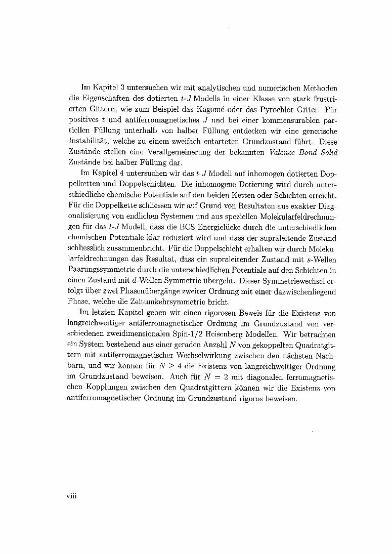
Im Kapitel 3 untersuchen wir mit analytischen und numerischen Methoden
die Eigenschaften des dotierten t-J Modells in einer Klasse von stark frustri¬
erten Gittern, wie zum Beispiel das Kagomé oder das Pyrochlor Gitter. Für
positives t und antiferromagnetisches J und bei einer kommensurablen par¬
tiellen Füllung unterhalb von halber Füllung entdecken wir eine generische
Instabilität, welche zu einem zweifach entarteten Grundzustand führt. Diese
Zustände stellen eine Verallgemeinerung der bekannten Valence Bond Solid
Zustände bei halber Füllung dar.
Im Kapitel 4 untersuchen wir das t-J Modell auf inhomogen dotierten Dop¬
pelketten und Doppelschichten. Die inhomogene Dotierung wird durch unter¬
schiedliche chemische Potentiale auf den beiden Ketten oder Schichten erreicht.
Für die Doppelkette schliessen wir auf Grund von Resultaten aus exakter Diag-
onalisierung von endlichen Systemen und aus speziellen Molekularfeldrechnun-
gen für das t-J Modell, dass die BCS Energielücke durch die unterschiedlichen
chemischen Potentiale klar reduziert wird und dass der supraleitende Zustand
schliesslich zusammenbricht. Für die Doppelschicht erhalten wir durch Moleku¬
larfeldrechnungen das Resultat, dass ein supraleitender Zustand mit s-Wellen
Paarungssymmetrie durch die unterschiedlichen Potentiale auf den Schichten in
einen Zustand mit d-Wellen Symmetrie übergeht. Dieser Symmetriewechscl er¬
folgt über zwei Phasenübergänge zweiter Ordnung mit einer dazwischenliegendPhase, welche die Zeitumkehrsymmetrie bricht.
Im letzten Kapitel geben wir einen rigorosen Beweis für die Existenz von
langreichweitiger antiferromagnetischer Ordnung im Grundzustand von ver¬
schiedenen zweidimensionalen Spin-1/2 Heisenberg Modellen. Wir betrachten
ein System bestehend aus einer geraden Anzahl N von gekoppelten Quadratgit¬tern mit antiferromagnetischer Wechselwirkung zwischen den nächsten Nach¬
barn, und wir können für N > 4 die Existenz von langreichweitiger Ordnungim Grundzustand beweisen. Auch für N = 2 mit diagonalen ferromagnetis-chen Kopplungen zwischen den Quadratgittern können wir die Existenz von
antiferromagnetischer Ordnung im Grundzustand rigoros beweisen.
viii

Contents
1 Introduction 1
1.1 A General Outline 1
1.2 From a multi-band Hubbard model to a single-band model...
6
1.3 From the single-band model to the mean-field model 9
2 Effective Interaction between the Inter-Penetrating Kagomé
Lattices in NaxCo02 17
2.1 Introduction 17
2.2 Tight-binding model 22
2.3 Coulomb interaction 27
2.4 SU(4) generators 30
2.5 Reduction of the symmetry 31
2.6 Ordering patterns 36
2.7 Possible instabilities 49
2.7.1 Coupling constants 49
2.7.2 Effect of the trigonal distortion 50
2.8 Na-superstructures 52
2.9 Wannicr functions 57
2.10 Superconductivity 59
2.11 Discussion and conclusion 61
3 Bond Order Wave Instabilities in Doped Frustrated Antiferro-
magnets 65
3.1 Introduction 65
3.2 Model and lattices 67
3.3 The limit of decoupled simplices 69
3.3.1 Approaching the uniform lattices 70
3.4 Doped quantum dimer model 72
ix
Contents
3.5 Mean-field discussion 74
3.5.1 "Supersolid" 80
3.6 Weak-coupling discussion 82
3.6.1 Kagomé strip 83
3.6.2 Checkerboard lattice 85
3.6.3 Kagomé lattice 90
3.7 Numerical results 91
3.7.1 Kagomé lattice 91
3.7.2 Checkerboard lattice 92
3.7.3 Kagomé strip 94
3.8 The Dirac points of the kagomé lattice 97
3.9 Discussion and conclusion 105
4 Inhomogeneously Doped t-J Ladder and Bilayer Systems 109
4.1 Introduction 109
4.2 Strong rung coupling limit Ill
4.3 Exact diagonalization 114
4.4 Renormalization group 117
4.5 Mean-field analysis for the t-J ladder 124
4.5.1 Spinon-holon decomposition 124
4.5.2 Mean-field results for the t-J ladder 127
4.6 Mean-field analysis for the bilayer 131
4.6.1 The symmetric bilayer 133
4.6.2 The inhomogeneously doped bilayer 134
4.7 Discussion and conclusion 137
5 Existence of Long Range Magnetic Order in the Ground State
of Two-Dimensional Spin-1/2 Heisenberg Antiferromagnets 139
5.1 Introduction 139
5.2 N layers with nearest-neighbor couplings 141
5.3 Bilaycr with ferromagnetic next-nearest-neighbor coupling ...144
5.4 Diagonal bilayer 150
5.5 Discussion and conclusion 153
A Appendix to Chapter 2 155
A.l Definitions of the pocket operators 155
A.2 Derivation of the effective Hamiltonian 155
A.3 The symmetry group G 157
x
Contents
B Appendix to Chapter 3 159
B.l RG analysis 159
B.l.l Kagomé strip 159
B.1.2 Checkerboard lattice 161
B.1.3 Weak-coupling on the honeycomb lattice 162
C Appendix to Chapter 5 167
C.l Anderson bound for the energy 167
C.2 Proof of Gaussian domination 168
Bibliography 169
Acknowledgments 179
Curriculum Vitae 181
xi

Chapter 1
Introduction
1.1 A General Outline
Strong correlations in low-dimensional electronic systems are responsible for
an almost inexhaustibly rich variety of phenomena. High-temperature super¬
conductivity and the fractional quantum Hall effect arc probably the most
prominent examples, but also magnetism in solids originates from the Coulomb
repulsion between the electrons. Ordering processes can be observed at low
temperatures that lead to phases with spontaneously broken symmetry but
also disordered and highly fluctuating liquid ground states like spin liquids or
Luttingcr liquids might describe the low energy physics of a material.
For a theoretical understanding of these different order and disorder phe¬
nomena the effective dimension of the system plays a crucial role. All solids
are three-dimensional (3D) but often the quantum mechanical models used to
describe the low-energy behavior are one-dimensional (ID) or two-dimensional
(2D).Due to the progress in materiel research many bulk materials containing ID
structures have been synthesized. Famous examples are the organic supercon¬
ductors, carbon nanotubes, spin-chain and ladder compounds [1]. In this thesis
we study in Chapter 4 the superconducting phases in inhomogeneously doped
ladder and bilayer systems. Note, that these superconducting phases in ID
systems that wc describe by a mean-field analysis can only be realized in mate¬
rials owing to the actual three-dimensionality of the solids and due to inevitable
weak interconnections between the ID structures. In a pure ID electron system
no continuous symmetry breaking can occur even in the ground state due to
the disordering effects of the quantum fluctuations. A discrete symmetry can
1

1. Introduction
be broken but as in this case no Goldstone mode appears the system usually
acquires a gap. Ungapped ID systems of interacting particles have peculiar
properties: One particle can not move independently of the other particles and
therefore the fundamental excitations of the system are collective excitations
rather than single-particle excitations. This insight led to the development of
the Bosonization technique, which is only one of several powerful theoretical
tools available in lD.a It turns out that at low energies these ungapped ID
systems form so-called Luttingcr liquids, which can be described by a universal
Hamiltonian with only two free parameters. The Luttinger liquids form the ID
analogue to the 3D Fermi liquid, in the sense that also the Fermi liquid theory
provides a universal low-energy theory for a 3D interacting Fermi system with¬
out broken symmetry.15 In 2D such a universal low-energy theory is still missing
and for this reason the 2D and quasi-2D materials provide the most exciting,
but probably also the most puzzling and controversial condensed matter sys¬
tems. Graphene is a recently found 2D semi-metallic allotrope of carbon that is
currently being intensively studied due to its possible technical applications [2].Its chiral fermionic excitations with linear dispersion reminding of the masslcss
Dirac spectrum have very recently been suggested to be a solid state imple¬
mentation of quantum electrodynamics in (2+1) dimension and, e.g., to allow
for an experimental test of the Klein paradox [3]. In Sec. 3.8 we analyze the
properties of the Dirac cones in the kagomé lattice and show how theoretical
results for the honeycomb lattice can be translated to the kagomé lattice [4, 5],
Another very interesting 2D material is the layered transition metal oxide
Na3;Co02- The attention of the strongly correlated electrons community was
especially focused on this material after the discovery of superconductivity in
the hydrated samples with x ks 0.35 [6], which came as big surprise after the
intense search for superconductivity in layered transition metal oxides. The
nature and the origin of the superconducting state are still not clarified, but
it was realized quickly that already the normal state of Na2;Co02 is very un¬
usual: At x — 0.5 a magnetic transition at 88 K is followed by a metal-insulator
transition at 53 K [7], and for larger values of x metallic behavior is coexisting
with local moments and Curie-Weiss susceptibility. At even higher Na con¬
centrations (x > 0.75) a spin-density wave instability occurs at 22 K [8]. One
aThis technique is also applied in this thesis for two different ID models in Sec. 3.6.1 and
in Sec. 4.4.
bIn contrast to the Luttinger liquid, the elementary excitations in a Fermi liquid are
single-particle excitations.
2
1.1. A General Outline
problem in the theoretical analysis of this model is posed by the Na ions that
provide a disordered charge background or impose superstructures with rather
large unit cells. A further complication arises due to the multi-orbital character
of the C0O2 plane consisting of three almost degenerate t2g orbitals on a Co
site. The first chapter of this thesis is devoted to this material. It contains
a derivation of an effective model for the orbital and spin degrees of freedom
of a single Co02 plane taking into account the multi-orbital aspect and the
Coulomb interaction.
Another important property of NaxCo02 is the fact that it is build up of
triangular lattices. The triangular lattice or any other lattice that contains
triangles is frustrated in the sense that no antiferromagnetic spin arrangement
with an opposite alignment of all neighboring spins is possible. Antiferro¬
magnetic spin systems on highly frustrated lattices are a relatively new and
fascinating research field [9]. In our work on Na;rCo02 we are confronted with
doped frustrated lattices and also in Chapter 3 we study doped highly frus¬
trated lattices like the kagomé or the pyrochlore lattice. In our study it turns
out that due to presence of charge degrees of freedom the frustration can be
avoided and an unfrustrated ground state can be obtained.
Many of these exotic phases and ordering phenomena described above only
exist at low temperatures. In fact the energy scale associated with their critical
temperatures are often several orders of magnitude lower than the energy scale
of the parameters in the microscopic models, like the Coulomb repulsion U and
the hopping integral t in the Hubbard model for example.
The derivation of an effective Hamiltonian that allows for a description
of the low-energy physics from the original microscopic Hamiltonian is one of
the most important and most challenging problems in theoretical solid state
physics. In the following we will present several alternatives for deriving such
effective low-energy theories and and point out where and in which context
these different methods where applied within this thesis:
The most direct method for such a derivation are based on the renormal-
ization group (RG) ideas. Usually, the implementation of these methods uses
a functional integral representation that allows to integrate out successively
high-energy degrees of freedom by renormalizing at the same time the inter¬
action between the low-energy degrees of freedom. The energy scale can be
reduced in discrete steps or in a continuous way and in the latter case it is
possible to obtain a set of differential equations that generate a flow of the ac¬
tion towards the effective low-energy action. The RG schemes are most easily
3
1. Introduction
derived for ID systems where the Fermi surface (FS) consists only of a discrete
set of points [10]. An alternative way to explore the low-energy correlations of
an interacting ID Fermi system is provided by the density matrix renormal-
ization grotip (DMRG) method which is a very modern numerical RG method
for ID systems [11]. In higher dimensions it is in special cases also possible
to restrict the RG analysis to the vicinities of a few selected points of the FS
[12, 13] but in general it is necessary to derive an RG scheme not only for a
set of coupling constants but for continuous coupling functions (functional RG)
[14, 15]. In this thesis we apply the RG equations for the two-leg ladder [16]
to a doped frustrated ID system (Sec. 3.6.1) and find good agreement with
numerical DMRG results (Sec. 3.7.3). We also compare our mean-field cal¬
culations for the inhomogeneously doped t-J ladder with a weak-coupling RG
analysis in Sec. 4.4. Furthermore, we use a simple RG scheme for the square
lattice to analyze the doped checkerboard lattice which is a 2D analog of the
3D pyrochlore lattice (Sec. 3.6.2).
For strong interactions and increasing dimensionality the RG schemes might
become intractable. An alternative way to derive an effective low-energy model
in any dimension is given for large Coulomb repulsion where we have the small
parameter A = t/U [17]. In this method, the Hilbert space is constrained to the
subspace M of lowest energy eigenstates of the interaction, which is usually
well separated from the higher-energy subspaces. The effective Hamiltonian is
then found by a canonical transformation, H = e~lSHelS, such that H is block
diagonal with respect to the subspace M and by a restriction of H to M.. In
first order of A the effective Hamiltonian consists just of the kinetic energy
hopping processes within the subspace M. In second order it contains also the
"virtual processes" of hopping out of and back into the subspace M. In this
way a new effective interaction at an intermediate energy scale J oc t2 jXJ can
be obtained. The disadvantage of such a reduced Hilbertspace are the awkward
commutation relations of the so-called Hubbard operators that must be intro¬
duced to enforce the constraint. An elegant reformulation of the problem can
be achieved if the Hubbard operators are replaced by products of a fermionic
and a bosonic particle [18].c These additional "slave" particles allow however
to study the system with a mean-field theory that takes the constraint at least
approximatively into account. In Chapter 4 we perform such a mean-field anal-
cNotc, that these particles are also not free fermions or bosons. The still have to fulfill a
local constraint.
4

1.1. A General Outline
ysis for the t-J modeld on inhomogeneously doped two-leg ladder and bilayer
systems. Furthermore, in Sec. 3.5 we study a different strong-coupling model,
the somewhat more general t-J-V model, on the kagomé and on the pyrochlore
lattice, accounting for the constraint by the statistical Gutzwiller mean-field
method. Note, that the mean-field analysis of the effective interaction goes
much further than a mean-field analysis of the original interaction, as due to
the canonical transformation new and longer range interaction terms appear
which lead to new types of mean-fields and to a bigger variety of possible in¬
stabilities.
The fact that the dimensionality of the Hilbertspace is drastically reduced in
the effective strong coupling models like the t-J model can be directly exploited
in ID and 2D. The exact diagonalization (ED) method allows to calculate the
ground state energy and correlation functions in the ground state exactly for
reasonably large systems (about 20 sites for the t-J model). We compare our
analytical or mean-field results against ED data for the t-J model in Sec. 3.7.1-
3.7.2 and in Sec. 4.3. This mutual comparison of complementary approaches
allows us to assure that the we describe intrinsic properties of the system and
not an artifact of the approximation or the finite size.
At fractional filling, i.e., if the number of electrons per unit cell is a simple
fraction, there exists often a unique charge distribution (up to translations) that
minimizes the interaction energy. In this case all charge excitations are gapped
and there are no terms of first order in A — t/U in the low-energy subspace.
The strong-coupling model describes then the effective second order interaction
between the remaining spin and orbital degrees of freedom. These models loose
their fermionic character as the interaction can be expressed through operators
that are quadratic in the original fermionic operators. The most prominent
example of such a model is the antiferromagnetic Heisenberg model obtained
for the half-filled large U Hubbard model. The redundancy of the description
of such a model with fermionic operators shows up in the local SU (2) gauge
symmetry of the interaction, which transforms the creation operators with down
spin into the annihilation operators with up spin but leaves the local spin
operators invariant [20]. The presence of this local gauge symmetry plays a
role close to half-filling [21], but exactly at half-filling the system reduces to a
pure spin model. The antiferromagnetic spin-1/2 Heisenberg models in 2D is
dThe t-J model was derived by Zhang and Rice [19] as an effective single-band model for
the high-Tc superconductors. It is similar but not identical to the strong coupling Hubbard
model.
5
1. Introduction
the topic of Chapter 5 which is the last chapter of this thesis. We address the
question, whether there exists antiferromagnetic long range order in the ground
state or whether the ground state is disordered due to quantum fluctuations.
For models on the hypercubic lattice this question can be rigorously answered
in any dimension except for 2D.e We do not manage to provide a rigorous proof
for the square lattice, but we give examples of spin-1/2 models on the bilayer
where long-range antiferromagnetic order can in fact be proven.
1.2 From a multi-band Hubbard model to a
single-band model
In the previous section we discussed the derivation of an effective interaction
for a strong-coupling model. In this section, we describe a straightforward pro¬
cedure to reduce a weak-coupling multi-band or multi-orbital Hubbard model
to a single band model. This procedure can be useful to describe correlated
metals and was applied in Chapter 2 to the multi-orbital system Naj;Co02.
A further application of this method is given in Chapter 3, where the weak-
coupling Hubbard model on bisimplex lattices was studied. We consider the
Hamiltonian
H = H0 + Hlnt. (1.1)
The quadratic part, H0, of the Hamiltonian for a general multi-band or multi-
orbital tight-binding model without spin-orbit coupling is of the form
^o-EEE (4-r' -^M &,<v*, = £ tf tUw, (i-2)rr' ij (T kvcr
where t^_T, is the transfer integral between the orbitals (atoms) i and j in the
unit cells at r and r' and ££ is the dispersion of the band v. Furthermore, H0
includes a chemical potential term proportional to fi. The operators jkl/a are
obtained by the orthogonal transformation 71^0- — ]T\- Oj^ciyv where c^ are
the Fourier transformed operators of cTia. The Hamiltonian //0 contains the
atomic energy of the orbitals the kinetic energy gain due to derealization and
the potential of crystalline lattice.
eThere is of course good numerical evidence that also the 2D ground state is ordered, but
a rigorous proof is still missing.
6

1.2. From a multi-band Hubbard model to a single-band model
The interaction part, Hini, of the Hamiltonian is given by
H** = \ ££££ ylji/j' 4r4,vwv*- (L3)r ij i'j' era'
It describes the screened Coulomb interaction between the electrons. Note,
that we restrict us here for simplicity to on-site interactions. In general also
nearest-neighbor or even longer range interactions can be treated in similar way,
as we will show for the extended Hubbard model on the checkerboard lattice in
Sec. 3.6.2. The single-orbital Hubbard model in a system with several sites in
a unit cell is obtained by the choice VrtJ't-7'' = 118^8^8^1. If a system has only
one atomic site per unit cell with several symmetry related orbitals, e.g., the
three £25 orbitals, the interaction (1.3) contains in addition to the intra-orbital
Coulomb repulsion, U, also an inter-orbital Coulomb repulsion, U'SijiSßi, a
Hund's coupling term, Jh8ü'8jj', and a pair hopping term, J'S^Syji* As the
interaction is local it leads to a momentum independent interaction in reciprocal
space. In the basis of the single-particle states c^a- the interaction Hamiltonian,
.Hint, simply reads as
^Int =2ÏV £ £££ V1JlJ cM<rck2jVck3iVck.u'<7- C1-4)
ki...k4 ij i'j' aa'
Due to the translational symmetry of the interaction the sum over the momenta
is restricted, i.e., the vector lq + k2 — k3 — k4 must be a reciprocal lattice vector,
which is indicated by the prime over the sum. We assume that the typical
interaction energies of Hïnt are much smaller than a typical bandwidth of the
quadratic Hamiltonian, H0. It is therefore convenient to express the interaction
Hamiltonian, H^t, in terms of the operators 7^ that describe the eigenstates
of Ho- This transformation leads to a momentum dependence of the interaction
Hamiltonian.
^Int = ^y 2^ Z-^Z-^Z^ ^ki...k4 7ki^,r7k2W'Tk3^'cr'7k4vV 0-^)
ki...k4 pv fi'u' <tg'
VCZ - ££oç&agagv&i' (i.e)ij i'j'
Such a multi-orbital Hubbard model is generally far too complicated for a fully-
fledged analytical treatment. A first substantial simplification can be achieved
It is of course also possible to describe the general situation with several atomic sites per
unit cell and several different orbitals on each site within this formalism.
7

1. Introduction
by restricting the system to a single band model. In general several bands ££will cross the Fermi energy and it will not be possible to choose one single band,
ß. However, it is possible to assign to every point k of the Brillouin zone a
band index v^ by the implicit definition
e-minl&l. (1.7)
If the different sheets (or lines) of the Fermi surface are well separated and if we
assume that the interaction is weak we can restrict our attention to the Hubert
space spanned by the operators 7kl/k(7 and still correctly describe the low-energy
physics of the system. We can now introduce the single-band notation as follows
& = £k% 7ka = 7k^a, and Vki...k4 = v£ï£* (L8)
and write down a single-band Hamiltonian
Hsh = £4 iLlUa +2N£ £ Vkl'"k4 7^7k2a'7k3,T'7k4CT- (1-9)
kcr kj...kii au'
Provided that the interactions are weak enough this single-band Hamiltonian,
/fsb, reproduces the low-energy physics of the original system accurately. We
showed that in weak coupling a single band description of a multi-band model is
possible. The momentum independent local interaction of the original Hamil¬
tonian will however acquire a momentum dependence in the single-band Hamil¬
tonian.
In certain cases, it is however possible to describe the momentum dependent
interaction approximately by a few constants. In a ID system for example the
Fermi surface consists of a discrete set of points. For each of the four vectors
kj in Eq. (1.6) we can associate the closest Fermi point and denote it with kFi.
For weak coupling the Eq. (1.6) can be approximated by
K.'Z = ££<og2<<^'iY (i-io)ij i'j'
This procedure was carried out for the ID kagomé strip in Sec. 3.6.1. In higher
dimensions a similar simplification is sometimes possible. For example if the
Fermi surface consists of individual hole or electron pockets, we can again
associate to each vector kj the closest pocket center kFj and find again through
Eq. 1.10 an effective interaction that does only depend on a few constants.
In Chapter 2 we show an application of this method to the 2D multi-orbital
system of a C0O2 plane.
8
1.3. From the single-band model to the mean-field model
In the special case where two bands ££ and ££ are symmetric about the Fermi
energy, i.e., if ££ — ±££, the association of a single band index to every vector
in the Brillouin zone as described in Eq. 1.7 is not possible. This situation
occurs for example in the 2D kagomé lattice at 1/3-filling. The derivation of a
single-band model is not possible in this case, but we show in Sec. 3.6.3 how an
effective two-band model can be derived from the original three-band model.
The single-band Hamiltonian derived in this way possesses still the full
symmetry of the systemg and does therefore not allow to detect the occurrence
of a spontaneous symmetry breaking. The mean-field approximation provides
a simple and widely applicable method for the detection and the description
of phases with spontaneously broken symmetry. As this thesis contains several
different mean-field approaches we provide in the following section an outline
of the standard mean-field analysis for a general single-band electronic lattice
model.
1.3 From the single-band model to the mean-
field model
The theoretical analysis of the single-band model, although much simpler than
the multi-band model, is still a formidable challenge. An often used and rather
drastic simplification of the problem can be achieved by the mean-field approx¬
imation. The mean-field theory is well suited to detect phases with sponta¬
neously broken symmetry where operators, whose expectation values are iden¬
tically zero for finite systems due to symmetry, acquire a finite expectation
value in the thermodynamic limit. The symmetry group of the system is spon¬
taneously reduced to a subgroup and the different subgroups characterize the
various possible phases. According to the presence or absence of the global U(l)
symmetry that guarantees the particle number conservation of the Hamiltonian
(l.l)h one distinguishes between particle-hole and particle-particle instabilities,
respectively. The basic idea of the mean-field theory is the assumption that
the ground state can be reasonably well described by a Slater determinant, i.e.,
that the ground state of the interacting system can be approximated by the
gAs the energy of the non-interacting state is the only selection criterion for the low-energy
subspace, this subspace and the restriction of the Hamiltonian to this subspace are invariant
under all symmetry operations of the system.
hHo and iïint are invariant under the global gauge transformation cricr —> e1¥,crjff.
9

1. Introduction
ground state, \ip), of a non-interacting (quadratic) Hamiltonian. In the ground
state \tp) the expectation value of an operator can be evaluated by applying
the Wick theorem, e.g., the expectation value of the interaction term in the
single-band model of Eq. (1.9) model is given by
V° =2NS £ Vk1...k4 f 7kl<r7k2,T'7k3<r'7k4tr
- 7kla7k3^7k2^7k4a +
ki...k4 oa'
+ 7k1Cr7k41T7k2^7k3^ j , (1-11)
where the operators that are connected by a brace stand for the ground-state
expectation values of these operators, e.g., 7k1(r7k20-' = (V,l7k1(77k2CT'|'0)- The
mean-field Hamiltonian
#MF = £ £k lll^a + 4 £' £ ^,..k4*-k4 - Vo (1.12)kcr ki...k4 aa'
0aa'k* = (7^^k2^7k3a'7k4a-7^k3a'7i2^7k4ff+7k^7k4a7k2(r'7kJ(T'+h.C.Jhas by construction the same expectation value in the ground state l^) as
the original Hamiltonian (1-9).1 The Hamiltonian HUf is quadratic and if
we replace the braced operators by a given set of complex numbers, we can
diagonalize HMF by a Bogoliubov transformation, calculate the expectation
values of the braced operators in this ground state and use these values as a
new set of complex numbers or mean-fields. This procedure can be iterated
until a self-consistent set of mean-fields is found. The ground-state energy of
the Hamiltonian Huv is extremal with respect to all mean-fields for a self-
consistent set of mean-fields. This follows directly from (1.12) and from the
Feynman-Hellman theorem. If several self-consistent solutions exist the one
with the lowest energy is chosen. If the ground-state does not break any of
the symmetries of the system, i.e., if it is invariant (up to a phase) under
all symmetry transformations, most of the mean-fields are identically zero.
The non-vanishing mean-fields only renormalize £k in the Hamiltonian (1.9)and will not produce any spectacular effect. In weak-coupling, these mean-
fields can even be neglected. In the following we will focus on the different
types of symmetry breaking mean-fields. Three different categories of symmetry
breaking mean-fields can be distinguished:
'We used the properties Vk1k2k3k4 = Vk2kakjk3 = Vk4k3k2k1 that follow from the commu¬
tation relations and from Hermicity.
10

1.3. From the single-band model to the mean-field model
Superconducting mean-fields are finite expectation values of 7k+q,cr'7-ka
for a fixed value of q. They break (at least) the U(l) gauge symmetry.
In the so-called Cooper channel the total momentum of the particle pair,
q, vanishes. The rather special case of finite q is called Fulde-Ferrell-
Larkin-Ovchinnikov pairing state and might be present in systems with
broken time-reversal symmetry. For the case where only superconducting
symmetry breaking mean-fields with momentum q are finite it is possible
to write down a reduced Hamiltonian that produces the same mean-field
behavior. This Hamiltonian only keeps a single channel of the interaction
in the original Hamiltonian (1.9) and is given by
i
#SC - £4 iLlka + TTJV ££ VW T-ka7k+q,«T'7k'+q,<r'7_k'«T» l1'13)ka kk' aa'
with Vkkl ~ ^-k,k+q,k'+q,-k'- In comparison to the original interaction the
sum over three independent momenta has been reduced to a sum over two
independent momenta, i.e., only an infinitesimal part of the terms in the
original interaction Hamiltonian is kept in the mean-field analysis, but
this infinitesimal fraction of terms can still provide an extensive contri¬
bution to the ground-state energy.
In the following discussion we set q — 0 as this is by far the most im¬
portant case and because in this case the Hamiltonian (1.13) is invariant
under all symmetry transformations of the original Hamiltonian (1.9).
Vkk! is invariant under the exchange of k and k' and under a simul¬
taneous sign change of k and k' but, in general, V^ is not invariant
under a sign change of a single vector. This invites to the decomposition
vw = Vk£'S + Vk5't-j The even P^t, Vw*> leads to singlet pairing and
the odd part, Vkk,'t, to triplet pairing. For q ~ 0 we have V^9k^n,kn — V^for all point group symmetry operations 1Z. From this invariance follows
that Vkk, must be a linear combination of the invariants associated with
each point group representation and that it can be written as
^-££^k< with vk5 = £A'via(k)^(k'). (i.i4)j a s
where the index j runs over all irreducible point group representations
and /gö(k) is a set of basis functions for the representation j. The index
%Ï'S = (V& + V^,)/2 and V^ = (V$ - V%.)/2.
11
1. Introduction
s runs from 1 to the dimension of the representation j. As there might be
different basis functions for a given representation we need the additional
index a that runs over the different realizations of the representation j.
This is similar to atomic physics where there are also different types of s
orbitals. On the hypercubic lattice, e.g., we have the functions /(k) = 1
and /(k) — ^Vcosfcj as different functions for the trivial representation.
The former is called s-wave and describes local pairing and the latter is
usually called extended s-wave and describes nearest-neighbor pairing.
The coefficients AJQ are called coupling constants. If the point group con¬
tains the inversion symmetry the decomposition (1.14) is compatible with
the singlet triplet decomposition. A spontaneous symmetry breaking can
only occur in the channels where the coupling constant AJO! is attractive,
i.e., Xja < 0,k The self-consistency requirement of the mean-field calcu¬
lation can be translated into a gap equation. The linearized version of
the gap equation allows to determine the critical temperature given by
Tc = max7T^. T-! is defined as the lowest temperature where the equa¬
tion #(k) — —'}2cls\:'afia(k)(fia,g)T has a non-trivial solution, g. For
£k — £-k the temperature dependent scalar product is defined as
(/,S)r4E»W^( (1.15)
which diverges logarithmically at low temperatures (Cooper instability).
If only one type of representation, j, exists in V^ the definition of the
Ti reduces to 1 — —AJ'(/|, f3s)Tj which is independent of s.
It is possible that superconducting mean-fields corresponding to two dif¬
ferent point group representations, e.g., s-wave and d-wave, are simulta¬
neously finite in the ground state. These systems do however not only
break the U(l) gauge symmetry, but the symmetry group of the system
will be reduced such that the combination of the different representations
is again a representation of the reduced symmetry group. Therefore,
such a ground-state is separated from the high-temperature phase with
full symmetry by two phase transitions.
For a single-band model derived from a multi-band model as described
in the previous section a spontaneous superconducting instability in such
kNote that the interaction is a sum over terms of the form Ajqj4JqJ4. and the expectation
value of such a term has the same sign as AJ'Q.
12

1.3. From the single-band model to the mean-field model
a mean-field analysis is generally not expected. As the original Coulomb
interaction is repulsive the electrons do not easily form bound states, i.e.,
most of the superconducting channels described above will be repulsive. It
can not be excluded that an attractive channel exists, e.g., a large Hund's
coupling term could produce a spontaneous superconducting instability
with triplet pairing, but in most cases the bare Coulomb interaction will
not be sufficient for the mean-field description of the superconductor.
In the spin-fluctuation theory for the high-Tc superconductors the bare
Coulomb interaction is replaced by an effective interaction, and Vkki con¬
tains a term which is roughly proportional to the spin correlation function
x(k — k'). This term that has a pronounced maximum at k — k' = (tt, it)
allows for a rf-wavc mean-field instability.
• Charge density wave (CDW) mean-fields are finite expectation values of
Ysa 7k+q,a7k(T f°r a &xed value of q. They can be viewed as pairing ampli¬
tudes in the particle-hole channel whereas superconductivity is produced
by pairing in the particle-particle channel. As in the superconducting
case it is possible to write down a reduced Hamiltonian for the CDW
instabilities that produces the same mean-field behavior. It is given by
#cdw - £ £k 7ka7ka + 4^££ V&? 7L7k+q)a7k'+q,<,'7k'a' (1-16)ku kk' aa'
with V&? = 2Vk)k/+q)k',k+q - Vk,k'+q,k+q,k'- The CDW instability breaks
translational symmetry. If the vector q is not a high-symmetry point
of the Brillouin zone that is invariant under all point group symmetries
(like the point (tt,ty) for the square lattice), the point group of (1.16) is
smaller than the original point group. With respect to this reduced point
group a symmetry decomposition of Vffi can be done as in Eq. (1.14).
Note, that CDW phases with even and with odd form factors ßa(k) arc
possible.
The critical temperature of the CDW instability can be calculated in the
same way as for the superconducting instability. Only the temperature
dependent scalar product has to be redefined as
U,9h -I E/(k)s(k)f^J, (LIT)
where fk = (e^T + 1)_1 is the Fermi function. Note, that for con¬
stant functions (f=g=l) the scalar product is given by the susceptibility
13
1. Introduction
X° and the critical temperature is determined by the Stoner criterion
1 = —AJxq- The susceptibility xq is generally not diverging at low tem¬
peratures. However, if the nesting condition £k+q = —£k is satisfied the
scalar product (1.17) reduces to the logarithmically diverging scalar prod¬
uct of Eq. (1.15).
The variety of CDW order parameters is very rich, especially if the form
factor is non-trivial: Staggered flux phases (e.g., ^-density waves) as well
as bond order waves can be understood within this formalism as CDW
phases. Starting from the repulsive Coulomb interaction we do not expect
to generate spontaneously a charge modulation and in fact we generally
obtain repulsive interaction in the mean-field Hamiltonians. If the original
interaction contains not only on-site but also nearest-neighbor repulsion
the CDW instabilities can occur spontaneously. In Sec. 3.6.2 we show
applying the procedure described above that for the checkerboard lattice
a CDW (or bond order wave) instability occurs.
But also from purely on-site Coulomb interactions it is possible to obtain
attractive CDW coupling constants as we show in Chapter 2 for the multi-
orbital model of NaaCo02. However, the CDW coupling constants are
not as attractive as the coupling constants of the spin density waves that
we discuss now.
• Spin density wave (SDW) mean-fields are finite expectation values of
(7k+q,î7kî — 7k+q,i7k|) f°r a nxed value of q.1 The SDW Hamiltonian
can be written as
#SDW = ££k7L7ka+^££ V$ <'lL%+q,all+qylv*' l1-18)k(T kk' era'
with Vkk, = —Vk,k'+q,k+q,k'- As we selected one of the three equiva¬
lent SDW order parameters the Hamiltonian (1.18) is not invariant un¬
der SU(2) transformations. The potential V^ can be decomposed as in
(1.14) according to the representations of the point group of the Hamil¬
tonian (1.18) which might be reduced for a finite vector q and the critical
temperature can be determined in the same way as for the CDW insta¬
bilities. The variety of the SDW phases is again very rich and ranges
!Due to the SU(2) invariance of our system we could equivalently choose (7t+q |7k| +
7k+q,i7kî) or i^k+qjTki ~ Tk+q,|7kî) for a discussion of the SDW states.
14

1.3. From the single-band model to the mean-field model
from a normal ferromagnet (q — 0) over antiferromagnetic phases to the
exotic phases containing staggered spin currents. Apart from the SU(2)
symmetry these phases usually break also time-reversal symmetry except
for the spin-current phases where time-reversal symmetry is broken in the
corresponding CDW phase. Due to the global minus sign in the definition
of Vjfk? the SDW coupling constants are usually attractive. In Chapter 2
a discussion of several SDW states for NaxCo02 with attractive coupling
constants is presented
The method described in this and in the previous section is a valuable approach
for a system with several electronic degrees of freedom in a single unit cell. If
the quadratic Hamiltonian, H0, is simple enough it is possible to derive the
single-band model analytically and to present it in a closed and explicit form.
In this way, the complexity of the problem can be reduced substantially and the
single band model can either be analyzed by the standard mean-field treatment
described above or can be studied by more sophisticated numerical or analytical
techniques. In any case, the mean-field analysis of the direct (zeroth-order)interaction provides important information about the dominant fluctuations
in the system. It is however important to remember, that these fluctuations
lead to effective interactions that might trigger also instabilities that are not
detectable directly in mean-field, e.g., a mean-field analysis of the Hubbard
can directly detect the antiferromagnetic fluctuations, but only after including
antiferromagnetic interactions in the Hamiltonian, superconductivity can be
obtained from the mean-field calculation.
15

Seite Leer /
Blank leaf

Chapter 2
Effective Interaction between
the Inter-Penetrating Kagomé
Lattices in NaxCoÜ2
2.1 Introduction
The layered Na;i;Co02 has been initially studied for its extraordinary thermo¬
electric properties and for its interesting dimensional crossover [22-25]. But re¬
cently wider attention has been triggered by the discovery of superconductivity
in hydratcd Nao.3sCo02 and the discovery of an insulating phase in Na0.5CoO2
[6, 26 -28]. Since then, various types of charge ordering phenomena in Na2;Co02
have been reported [29-43], but also strong spin-fluctuations and spin density
wave transitions have been observed [7, 8, 44-56].
The structure of the material of Naa;Co02 is shown in Fig. 2.1. It consists
of Co02-layers where Co-ions are enclosed in edge-sharing O-octahedra. These
layers alternate with the Na-ion layers with Na entering as Na1+ and donating
one electron each to the Co02-layer. Due to the crystal field splitting produced
by the O-octahedra, the Co 3d orbitals are split into the lower t2g orbitals and
the higher eg orbitals. Local density approximation (LDA) calculations show
that the t2g bands are clearly separated from the higher eg bands and from
the lower oxygen p bands. The total bandwidth of the t2g band is 1.6 eV [57],and the Fermi energy lies close to the top of the t2g bands. Note, that the
formal valence of the Co-ions is (4 — x)+, and that a Co3+ ion has a completely
filled t2g shell, such that x — 1 and x = 0 correspond to a band-insulating and
17

2. Effective Interaction between the Kagomé Lattices in NaxCo02
Figure 2.1: The structure of Naa;Co02 can be viewed as close-packed
stacking of triangular layers. The stacking within a unit cell is given by
Ao-BCo-Co-(A,B)Na-Co-BCo~Ao-{B,C)Na, where the letters A, B, and
C denote the three different types of triangular layers. The Na positions are only
partially occupied and neighboring Nal and Na2 sites can not be simultaneously
occupied. The Co-ions are coordinated by edge-sharing oxygen octahedra.
18

2.1. Introduction
a Mott-insulating filling, respectively. The electronic properties are therefore
dominated by the 3d-t2g electrons of the Co-ions which form a two-dimensional
triangular lattice. However, the spatial arrangement of the Na1+-ions plays a
crucial role too for the physics of this material. There are two basic positions
for the Na-ions, one directly above or below a Co-site and another in a center
position of a triangle spanned by the Co-lattice (cf. Fig. 2.1). The metallic
properties are unusual and vary with the Na-concentration and arrangement.
A brief overview of the present knowledge of the phase diagram of NaxCo02
shown in Fig. 2.2 leads to following still rough picture. The most salient and
robust feature, at first sight is the charge ordered phase for x = 0.5 separating
the Na-poor from the Na-rich system. At this particular filling the Na-ions
arrange along zig-zag chains already at 100 K, reducing the crystal symme¬
try from hexagonal to orthorhombic [29]. This Na pattern might induce also
the magnetic transition at Tx = 88 K and the metal-insulator transition at
TMl = 53 K, which could be clearly identified by magnetic resonance, transport
and susceptibility measurements [7]. Neutron scattering measurements pro¬
pose that the magnetic instability leads to an antiferromagnetic structure with
rows of ordered and non-ordered Co-ions where the ordered ions have staggered
inplane magnetic moments [58, 59],
On the Na-poor side (x < 0.5) the compound behaves like a paramagnetic
metal. When it is intercalated with H20 superconductivity appears at about
5K between x & 0.25 and x & 0.35. The symmetry of the superconducting
order parameter is not yet clarified, but it is probably unconventional and
maybe even spin triplet superconductivity [60].
On the Na-rich side one finds a so-called Curie-Weiss metal. Here the
magnetic susceptibility displays a pronounced Curie-Weiss-like behavior after
subtracting an underlying temperature independent part: x ~ C/(T—@) where
0 ranges roughly between -50 K and -200 K depending on x, and the Curie
constant is consistent with a magnetic moment in the range of (1- 1.7) //b per
formula unit. Deviations from the Curie-Weiss behavior have been observed at
low temperatures [61], and evidence for strong low-energy spin fluctuations that
can be suppressed by a magnetic field have been reported [37], A transition at
high temperature ~ 250 - 340 K has been observed and interpreted as charge
ordering [35, 38, 48].For even higher Na concentrations, x > 0.75, a magnetic transition occurs
at 22 K, which is most likely a commensurate spin density wave [47-50]. Neu¬
tron scattering experiments find ferromagnetic correlations in the layers and
19

2. Effective Interaction between the Kagomé Lattices in NaxCoQ2
1/4 1/3 1/2 2/3 3/4
Na Content x
Figure 2.2: The phase diagram for NaxCo02 from Ref. [27].
antiferromagnetic correlations perpendicular to the layers which is consistent
with an A-type antiferromagnetic ordering. Furthermore they show that the
magnetic fluctuations are highly three dimensional [45]. Interestingly, this mag¬
netic phase is metallic and has even a higher mobility than the non-magnetic
phase.
The arrangement of the Na-ions between the layers depends on the Na
doping x and several superstructures have been found [29, 30], The clearest
evidence for the superstructure formation is at x = 0.5 where the Na-ordering
leads to the metal-insulator transition at low temperatures [27, 28, 32]. But also
away from x = 0.5, nuclear magnetic resonance (NMR) experiments indicate
the existence of non equivalent cobalt sites and of nanoscopic phase separation
[34, 36].The complex interplay between Na-arrangement and the electronic prop-
20
2.1. Introduction
erties poses an interesting problem. Various theoretical studies have mainly
focused on single-band models on the frustrated triangular lattice, in particular
in connection with the superconducting phase ignoring Na-potentials [62-68],
There is also work done on multi-orbital models [60, 69, 70] and density func¬
tional calculations have been performed [57, 71-77]. According to the LDA
calculations the Fermi surface, which lies close to the top of the 3d-t2g-bands,
forms a large hole-like Fermi surface of predominantly a\g character. This re¬
sult is in agreement with angle-resolved photoemission spectroscopy (ARPES)
experiments [78-82]. In addition the LDA calculations suggest, that smaller
hole pockets with mixed aig and e'g character exist on the T-K direction on
the Na-poor side, however, so far the existence of these pockets has not been
confirmed with ARPES.
At the T point the states with a\g and e'g symmetry are clearly split, but
on average over the entire Brillouin zone the mixing between a\g and e'g is
substantial. Koshibae and Maekawa argued that the splitting at the T point
originates from the cobalt-oxygen hybridization rather than from a crystal field
effect due to the distortion of the oxygen octahedra, because the crystal field
effect in a simple ionic picture would lead to the opposite splitting of the aig and
e'g states [69]. There is also spectral evidence, that the low-energy excitations
of Na^Co02 have significant 0-2p character [83]. Reproducing the LDA Fermi
surface with a tight-binding fit for the cobalt t2g orbitals, it turns out that
the direct overlap integral between the cobalt orbitals is much smaller than
the indirect hopping integral over the oxygen 2p orbitals [70], Therefore, it
is reasonable to start with a three band tight-binding model of degenerate
t2g orbitals, where the only hopping processes are indirect hopping processes
over intermediate oxygen orbitals. This approximation provides an interesting
system of four independent and inter-penetrating kagomc lattices as it was
already pointed out by Koshibae and Maekawa [69],
Our study is based on this tight-binding model band structure which has
a high symmetry. Within this model we examine various forms of order that
could be possible from onsite Coulomb interaction. This chapter is organized
as follows: In Sec. 2.2, the tight-binding model and the concepts of kagomé
operators and pocket operators are introduced. In section 2.3 an effective
Hamiltonian for the local Coulomb interaction is derived and in Sec. 2.4 this
effective interaction is written in a diagonal form, by choosing an appropriate
basis of SU(4) generators. Sec. 2.5 deals with the effects of small deviations
from our simplified tight-binding model and in Sec. 2.6, all possible charge and
21

2. Effective Interaction between the Kagomé Lattices in NaxCoQ2
spin ordering patterns of our model and the corresponding phase transitions are
shortly described. Sec. 2.7 contains a discussion of the relevance of the above
described collective degrees of freedom to NaxCo02 comparing the different
coupling constants and by taking into account symmetry lowering effects and in
Sec. 2.8 we apply our model to the Na-ordering observed at x = 0.5. Sec. 2.9 is
dedicated to the local degrees of freedom (Wannier functions) in our model and
Sec. 2.10 discusses the decoupling of the effective interaction into the possible
superconducting channels. We summarize and conclude in Sec. 2.11. The major
part of the results in this chapter are published in Ref. [84] and Ref. [85].
2.2 Tight-binding model
We base our model on the assumption that the 3d-t2g orbitals on the Co-ions
are degenerate. Their electrons disperse only via 7r-hybridization with the in¬
termediate oxygens occupying the surrounding octahedra (Fig. 2.3). As noticed
by Koshibae and Maekawa the resulting electronic structure corresponds to a
system of four decoupled equivalent electron systems of electrons hopping on
a kagomé lattice [69]. The different sites of a kagomé lattice, however, are
represented by different orbitals. Each of the three orbitals {dyz,dzx,dxy} on
a given site participates in one kagomé lattice, and the fourth kagomé lattice
has a void on this site. A schematic representation of how the t2g orbitals on a
triangular lattice are grouped into four kagomé lattices is shown in Fig. 2.4.
The corresponding tight-binding model has the following form,
Htb ~ 2_j 2_>^ CkmaCkmV> f2-1)kir mm'
where ckma =
-7= X)r eïkTctm are tne operators in momentum space of c\ma
which creates a t2g orbital (dyz, dzx, dxy) with index m = 1, 2, 3 and spin a =î, |
on the cobalt-site r. N is the number of Co-sites in the lattice. The matrix
(—ß
2tcosfc3 2tcosk2 \
2tcosA;3 —11 2£cosfci , (2.2)
2tcos/c2 2tcosA;i —ji )
with ki = k • aj, cf. Fig. 2.3. The hopping parameter t = t2pd/'A > 0, where
tpd is the hopping integral between the py and the dxy or dyz orbital shown in
22
2.2. Tight-binding model
X
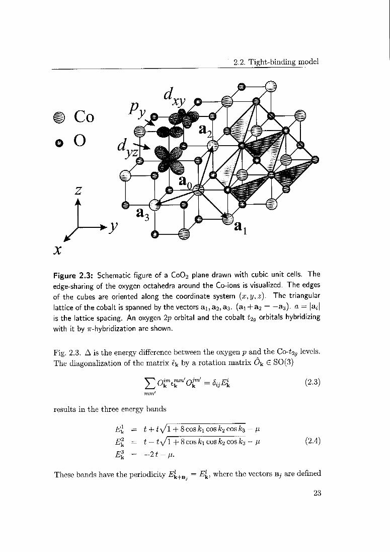
Figure 2.3: Schematic figure of a Co02 plane drawn with cubic unit cells. The
edge-sharing of the oxygen octahedra around the Co-ions is visualized. The edges
of the cubes are oriented along the coordinate system (x,y,z). The triangular
lattice of the cobalt is spanned by the vectors a!,a2,a3. (ai+a2 = —a3). a= |a»|
is the lattice spacing. An oxygen 2p orbital and the cobalt t2g orbitals hybridizing
with it by 7r-hybridization are shown.
Fig.2.3. A is the energy
difference between the oxygen p and the Co-t2g levels.
mi 1- " n ,1~"- —-J--:--êk
by a rotation matrix Ôk G SO(3)
(2.3)
J- 16. i.U. i-i ID LUG CliCJ-SJ LIHICICIILC UL
The diagonalization of the matrix
êk
Y,okmer'oir' = ^4mm'
results in the three energy bands
Ek = t + ty/l + 8 cos k\ cos k2 cos fc3 — /i
Ek = t — ty/l + 8 cos fci cos k2 cos k3 — /j,
El = -2t-p.
These bands have the periodicity Ek+B. — Elk, where the vectors Bj are defined
(2.4)
23
2. Effective Interaction between the Kagomé Lattices in Na;j;Co02
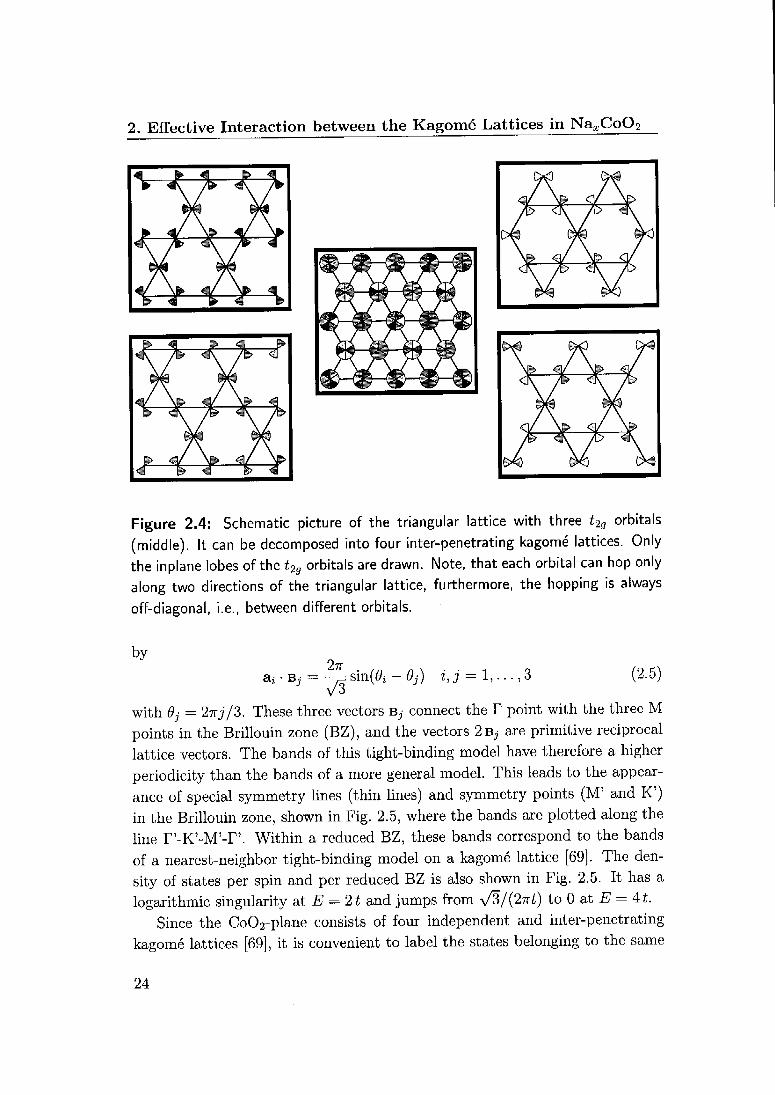
Figure 2.4: Schematic picture of the triangular lattice with three t2g orbitals
(middle). It can be decomposed into four inter-penetrating kagomé lattices. Only
the inplane lobes of the t2g orbitals are drawn. Note, that each orbital can hop only
along two directions of the triangular lattice, furthermore, the hopping is always
off-diagonal, i.e., between different orbitals.
by
aj • Bj = -j= sin(6>i - 9j) i, j = 1,..., 3 (2.5)
with 6j = 27T?'/3. These three vectors Bj connect the T point with the three M
points in the Brillouin zone (BZ), and the vectors 2bj are primitive reciprocal
lattice vectors. The bands of this tight-binding model have therefore a higher
periodicity than the bands of a more general model. This leads to the appear¬
ance of special symmetry lines (thin lines) and symmetry points (M' and K')
in the Brillouin zone, shown in Fig. 2.5, where the bands are plotted along the
line T'-K'-M'-r'. Within a reduced BZ, these bands correspond to the bands
of a nearest-neighbor tight-binding model on a kagomé lattice [69]. The den¬
sity of states per spin and per reduced BZ is also shown in Fig. 2.5. It has a
logarithmic singularity at E = 2t and jumps from \/3/(27rt) to 0 at E = At.
Since the Co02-plane consists of four independent and inter-penetrating
kagomé lattices [69], it is convenient to label the states belonging to the same
24
2.2. Tight-binding model
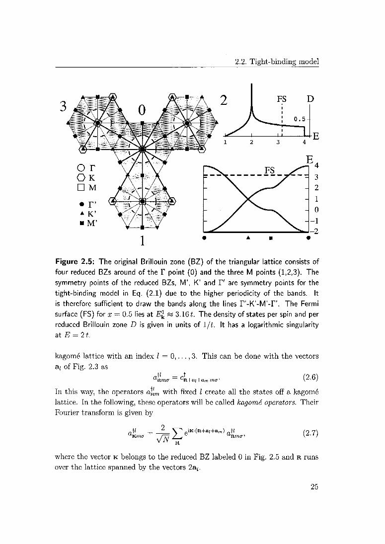
Figure 2.5: The original Brillouin zone (BZ) of the triangular lattice consists of
four reduced BZs around of the F point (0) and the three M points (1,2,3). The
symmetry points of the reduced BZs, M', K' and r" are symmetry points for the
tight-binding model in Eq. (2.1) due to the higher periodicity of the bands. It
is therefore sufficient to draw the bands along the lines T'-K'-M'-r'. The Fermi
surface (FS) for x = 0.5 lies at Ek « 3.16t. The density of states per spin and per
reduced Brillouin zone D is given in units of Xft. It has a logarithmic singularity
at E = 2t.
kagomé lattice with an index I — 0,..., 3. This can be done with the vectors
a; of Fig. 2.3 as
aRrna ~ CR+a;+amma* l^-DJ
In this way, the operators a^ with fixed / create all the states off a kagomélattice. In the following, these operators will be called kagomé operators. Their
Fourier transform is given by
—y iK-(R+a,+am) ffc "Timer i (2.7)
where the vector K belongs to the reduced BZ labeled 0 in Fig. 2.5 and r runs
over the lattice spanned by the vectors 2aj.
25

2. Effective Interaction between the Kagomé Lattices in NaxCoQ2
The BZ consists of four reduced BZs shown in Fig. 2.5. An alternative
labeling of the states is obtained therefore by defining the operators
where the vectors Bj are defined in Eq. (2.5) and in addition we set b0 — 0.
As shown in Eq. (A.l) in App. A, the transformation between the kagomé
operators a« and the pocket operators 6k corresponds to a discrete Fourier
transformation of a 2 x 2 lattice, and is given by
h\i -iV^fl*1 =Vjr-iat' (2 9)
UKma — n / jaKma / /J^Kirori \*"J)
1I I
where we have defined the symmetric and orthogonal 4x4 matrix
^1 = ^ = ^1 =^ = ^^- (2.10)
Note that the matrix elements of F are ±1/2, as the scalar products b., • a; of
Eq. (2.5) equal 0 or ±vr.
The tight-binding Hamiltonian (2.1) is diagonal in the pocket indices j (cf.
Appendix A Eq. (A.2)),
fftb = EEfKm'CCv (2-ii)iKa mm'
From this expression it is apparent, that the tight-binding Hamiltonian is in¬
variant under any U(4) transformation of the of the form
Ï
Eq. (2.9) is just a special case of Eq. (2.12). This shows that Htb is also diagonal
in the kagomé indices.
It is important to notice that the transformations in Eq. (2.12) involves
symmetries that are not present in a more general tight-binding model. For
example a finite hopping integral £</d due to the a-hybridization between neigh¬
boring t2g orbitals would break this symmetry. We will discuss this aspect below
in more detail and remain for the time being in this high-symmetry situation.
In Na;cCo02 the lower two bands are completely filled and will be quite inert.
For this reason in the following sections we will only deal with the operators of
the top band Ek whose operators are denoted as
<& = £0imaL- and C = E°Km^ (2-13)m m
26

2.3. Coulomb interaction
respectively, where 0^m are matrix elements of the rotation matrix 0K of
Eq. (2.3).The top band gives rise to four identical Fermi surface pockets in the BZ,
one in the T point and three at the M points. A translation in the reciprocal
space by the vectors Bj maps the pocket around the T point onto a pocket
around the M point. However, this fact does not lead to nesting singularities
in the susceptibility because a hole pocket is mapped onto a hole pocket by the
vector Bj. The susceptibility of the top band is given by
vo = _! V^ ^k+q ~ ^k ^lv -/Wq ~ /K to u)Xq N^El-Ek+cl N^E^-E^
K- )
where fk = f[ß(Ek - n)] and / is the Fermi function. In the last expression
of Eq. (2.14) the sum over k is restricted to the reduced BZ. The momentum
q also lies in the reduced BZ and is given by q = q + Bj. The susceptibility
-^ — ^o is periodic with respect to the reduced BZ and is just four times the
susceptibility of a single kagomé lattice. As we have almost circular hole pockets
with quadratic dispersion around the T and the M points, the susceptibility is
therefore approximately given by the susceptibility of the free electron gas in
two dimensions within each reduced BZ, with circular plateaus of radius 2Kp
around the F and the three M points.
2.3 Coulomb interaction
In this section we introduce the Coulomb interaction between the electrons. As
we have spin and orbital degrees of freedom, the on-site Coulomb interaction
consists of intra-orbital repulsion U, inter-orbital repulsion U', Hund's coupling
Jn and a pair hopping term J'. These parameters are related by U rj U' + 2JH
and Jh = J', where the first relation is exact for spherical symmetry. We can
write the onsite Coulomb interaction as
jji
Hr = U^nrm]nrmi + Y E E"rm^rmV
m m^m' aa1
+~2 ^ / /rm/rmVWViT (2.15)
m^m' aa'
2
i
cy / j / jCrma^rma' rm'a' rm'ai
m^m' a^a'
27

2. Effective Interaction between the Kagomé Lattices in Naa;Co02
where nrm(T = clm(7cTma. We obtain an effective Hamiltonian for the Coulomb
interaction by rewriting the Hamiltonian in terms of the pocket operators of
the top band &L defined in Eq. (2.13). For small re = |k|o we can expand
Eq. (2.13) in powers of n2 and obtain up to terms of the order k2
& =
TTfE f1 + Y2cosW~ 0m)]) ^' (2-16)
*m
^
where 0m = 2-KmjZ. Expanding the energy of the top band around the point
T', we obtain
el = t~K
2K K
k2 + Î2-3^COs(W) + 0(k) (2.17)
This shows that the pockets around the points V are almost perfectly circular.
The radius nF/a of these pockets depends on the Na doping x. Note that x
corresponds to the density of carriers with x — 1 giving a completely filled top
band. We have kf — 7r(l — x)/\/3. For the interaction in weak coupling and at
low temperatures, the states near the Ferini surface are important. For these
states and for not too small Na doping x we can neglect the second term in
the parenthesis of Eq. (2.16) compared to 1. Note, that this condition on x
is not very restrictive. Even for x = 0.35 the second term together with all
higher order terms is on the average one order of magnitude smaller than 1.
Dropping the second term in Eq. (2.16) spreads the a\g symmetry of the states
&k«7> which is exact only for k = 0, to all relevant states in the top band. The
interaction (2.15) can now be rewritten in terms of the a\g symmetric operators
b\ia- Processes involving states of the filled lower bands are dropped. The
dropping of the second term in the parenthesis of Eq. (2.16) is a considerable
simplification because it removes all K-dependence of the potential.
At this point it is convenient to introduce density and spin density operators
for the pocket operators of the top band:
4E6K^6L, (2-18)nlN
KO-
NKaa'
where a is a vector consisting of the three Pauli matrices. The resulting effective
interaction can be expressed with these operators in the following way
H* ^ ^EE (Bhi Sg • S'-fcQ + \ßt]kl h% n%^ . (2.19)Q ijkl
28

2.3. Coulomb interaction
Table 2.1: The coefficients of Eq. (2.20).
9C - -3E7 + 2J' + 2JH + 2U' 9D = +ZU + 6J' - 2JH - 2U'
9EC = +ZU - 2J' - 10JH + 14*7' 9E« = -ZU + 23' - 6JH + 2U'
9FC = +ZU - 2J' + 14JH - 10U' 9FS = -ZU + 2J' + 2JH - 6*7'
The symbols Bc/S depend on the Coulomb integrals and are given by
Bfkl = ±C{28ijkl - e2jkl) ± D8u8jk + Ec%8kl + FcHik8jh (2.20)
where the 8 (e2) symbol equals 1, if all the indices are equal (different) and 0
otherwise. The coefficients C, D, Ec>\ and Fc/S are listed in Table 2.1. Note,
that for small pockets, the momenta k of the pocket operators lPK in the four
fermion terms of Eq. (2.19) can not add up to a half a reciprocal lattice vector
Bj. In order to conserve momentum they must therefore add up to zero. Due
to the position of the pockets in the BZ, Umklapp processes with low energy
transfer are however possible for arbitrary small pockets. In fact, the processes
proportional to tf-kl and 8u8jk(l —%) are Umklapp processes, as Bj—Bj+B; — Bk
is a non-vanishing reciprocal lattice vector for e^^ ^ 0 and for 8u8jk(l—Sij) ^ 0,
and from Eq. (2.8) the momentum created by the operator 6k is k + b^-.
Some details about the derivation of Eq. (2.19) are provided in App. A.2.
There are different ways of writing this interaction in terms of the operators in
(2.18). Our formulation treats charge and spin degrees of freedom on an equal
footing. It corresponds to the decomposition of a Hubbard interaction n^ni
into \{\n2 - S • S).In order to express the effective interaction Hamiltonian of Eq. (2.19) in
terms of the kagomé operators, oKcr, we define spin and charge density operators
from the kagomé operators a'KCF as in Eq. (2.18).
^EaK+Q.<, (2.21)KU
_2_ y^ t* j
AT 2-J aK+Qa(Taa' aKa'
Kaa'
Note, that the density operators, which are defined from the pocket operators
feJdr are marked by a hat. The effective Hamiltonian, He^: of Eq. (2.19) can be
n,u _
.
o»j —
29

2. Effective Interaction between the Kagomé Lattices in Na^CoOjj
rewritten as
q ijkl^ '
From Eq. (2.9) and (2.10) follows that
%jkl~
Z_^ 'im-'jnJ~koJ~lpBmno
rnnop'
mnop
The symbols Ac/S turn out to have a simpler structure, given by
Ac
Ah
Q- -^8l]ki + J'8ü8]k + (2U' - Jn)8lJ8ki +
+ (2JH - U')8lk83l
Q+ ~^8l]ki — J 8ü8jk — J}i8tj8ki — U 8lk8ß
(2.22)
(2.23)
(2.24)
2.4 SU(4) generators
The tight-binding Hamiltonian described m Sec. 2.2 has a U(4) symmetry, re¬
flecting the fact that it consists of 4 independent and equivalent kagomé lattices.
The correlations introduced by the on-site Coulomb repulsion in Eq. (2 15)
breaks this symmetry and leads to interaction between orbitals belonging to
different kagomé lattices, as the three t2g orbitals on a given Co-site belong
to three different kagomé lattices. The effective Hamiltonian in Eq. (2.19) is
not invariant under general U(4) transformations, but is still invariant under a
finite subgroup of U(4). The symbols AcJskl defined in Eq. (2.24) are invariant
under permutation of the indices, i.e.,
As/C_
WcAijk\
—
AV{x)V{3)V{k)Vi}.)-'VeSA. (2.25)
From this follows that even including Coulomb interactions the symmetiic
group <S4 is a subgroup of the symmetry group of our system, G. Multiply¬
ing all operators a'K0. with the same kagomé index / by — 1 also leaves the
Hamiltonian, i7eff, invariant, because the symbols Ac%kl arc nonzero only if the
four indices ijkl are pairwise equal. These two different symmetry operations
generate a group with 384 elements. This group G is isomorphic to the sym¬
metry group of the four-dimensional hypercube. In App. A.3 the structure of
the group G is discussed and the character table is shown in Table A.l.
30
2.5. Reduction of the symmetry
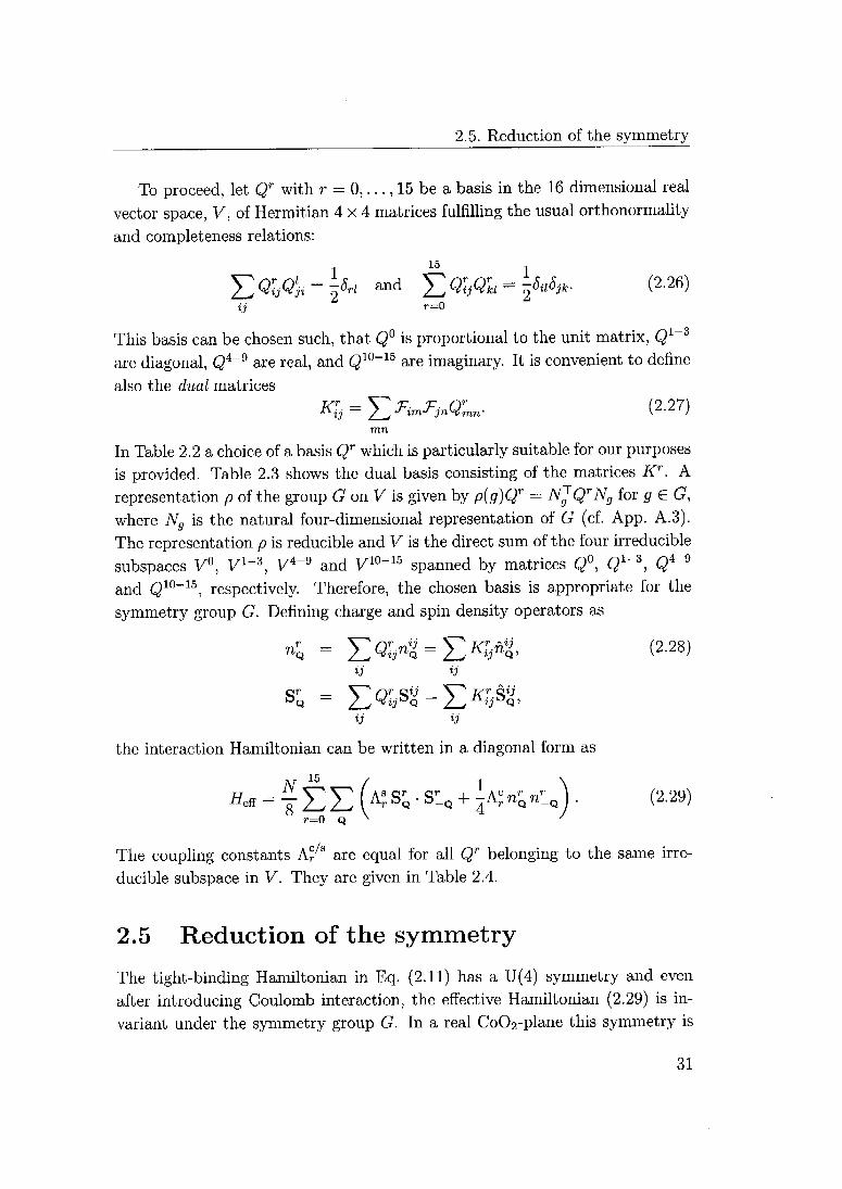
To proceed, let Qr with r = 0,..., 15 be a basis in the 16 dimensional real
vector space, V, of Hermitian 4x4 matrices fulfilling the usual orthonormality
and completeness relations:
115
1
Eq<ä = ^w and E^^ = 2^fc- (2,26)
ij r=0
This basis can be chosen such, that Q° is proportional to the unit matrix, Qx~z
arc diagonal, Q4"9 are real, and Q10"15 are imaginary. It is convenient to define
also the dual matrices
^ = E^><?- <2-27)mn
In Table 2.2 a choice of a basis Qr which is particularly suitable for our purposes
is provided. Table 2.3 shows the dual basis consisting of the matrices KT. A
representation p of the group G on V is given by p(g)Qr = NjQrNg for g G G,
where Ng is the natural four-dimensional representation of G (cf. App. A.3).
The representation p is reducible and V is the direct sum of the four irreducible
subspaccs V°, V1"3, V4"9 and V10"15 spanned by matrices Q°, Q1"3, Q4"9
and <210~15, respectively. Therefore, the chosen basis is appropriate for the
symmetry group G. Defining charge and spin density operators as
"q = Y.%< = Y,K^i (2-28)ij V
ij ij
the interaction Hamiltonian can be written in a diagonal form as
H<* = f EE (5 SQ • S-Q + IA^ < n-o) (2-29)
The coupling constants A£ are equal for all Of belonging to the same irre¬
ducible subspace in V. They are given in Table 2.4.
2.5 Reduction of the symmetry
The tight-binding Hamiltonian in Eq. (2.11) has a U(4) symmetry and even
after introducing Coulomb interaction, the effective Hamiltonian (2.29) is in¬
variant under the symmetry group G. In a real Co02-plane this symmetry is
31
2. Effective Interaction between the Kagomé Lattices in Naa;Co02
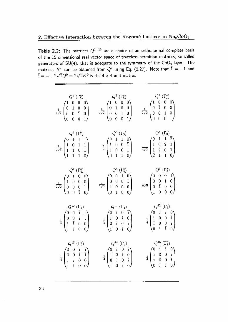
Table 2.2: The matrices Q1-15 are a choice of an orthonormal complete basis
of the 15 dimensional real vector space of traceless hermitian matrices, so-called
generators of SU(4), that is adequate to the symmetry of the Co02-layer. The
matrices Kr can be obtained from Qf using Eq. (2.27). Note that ï = — 1 and
I - -i. 2y/2Q° = 2V2K0 is the 4 x 4 unit matrix.
1
2v/2
Q1 (rg)/1 0 0 o\
0100
0 0 ï 0
\o 0 0 i)
1
2V6
Q" (rl)/o 1 1 1\
1011
1101
\i 1 1 0/
1
2V2
Q7 (il)/o 1 0 o\
1000
0 0 0 ï
\0 0 I 0/
1
A
Q10 (r4)/0 0 i i\
0 0 i i
i 1 0 0
\ï i 0 0/
1
4
QVi (rg)/o 0 ï ï\
0 0 i i
i i 0 0
V i 0 0/
1
ïs/ï
1
2V2
Q2 (rt)
/1 0 0 o\0 ï 0 0
0010
\o 0 0 ï/
Q5 (r3)
^0110^1 0 0 ï
ï 0 0 1
Vo ï 1 0/
Q8 (ri)
^0 0 1 0\0 0 0 ï
10 0 0
Vo ï 0 0/
Q11 (r4)
/0 i 0 ï\i 0 i 0
0 i 0 i
Vi 0 I 0/
QU m)
/0 i 0 i\i 0 i 0
0 ï 0 ï
Vi 0 i 0/
1
2V2
1
4V^
1
2V2
q3 (rg)
/1 0 0 o\0 ï 0 0
0 0 ï 0
Vo 0 0 i/
Q6 (r3)
/0 1 1 2\10 2 1
12 0 1
\2 1 1 0/
Q9 (r|)
/o 0 0 1^0 0 ï 0
0 ï 0 0
Vi 0 0 0/
Q12 (r4)
^0 i i o\i 0 0 1
i 0 0 i
V0 i I 0/
q15 (n)
/0 i i 0\i 0 0 i
i 0 0 i
Vo î î 0/
32

2.5. Reduction of the symmetry
Table 2.3: The matrices if1-15 are a choice of an orthonormal complete basis
of the 15 dimensional real vector space of traceless hermitian matrices, so-called
generators of SU(4), that is adequate to the symmetry of the Co02-layer. The
matrices Qr can be obtained from Kr using Eq. (2.27). Note that ï — —1 and
I = -i. 2y/2Q° = 2y/2K° is the 4 x 4 unit matrix.
1
2\/2
Kl (rg)/0 1 0 0^10 0 0
0 0 0 1
\o 0 1 0^
1
2^2
^2 (rt)/0 0 1 0^0 0 0 1
10 0 0
Vo i o o^
1 ^2v^
/v3 (rg)/0 0 0 1\
0 0 10
0 10 0
Vi 0 0 oy
1
2V6
K4 {!*)/3 0 0 0\
0 ï 0 0
0 0 ï 0
Vo o o v
1
2
k5 (r3)/0 0 0 0\
0 10 0
0 0 ï 0
\0 0 0 Oyi
1
2v/3
K6 (r3)/o 0 0 o\
0100
0010
\o 0 0 2/
1
2\/2
K7 (It)/0 1 0 0\
10 0 0
0 0 0 ï
Vo o ï o)
1
2v^
K» (Tb5)/0 0 1 0\
0 0 0 ï
10 0 0
\0 ï 0 0^
1
2V2
K» (I*)/0 0 0 1\
0 0 10
0 ï 0 0
y 0 0 oy
1
2
kw (r4)/0 0 0 0\
0 0 0 0
0 0 0 i
V) o I o/
1
2
#n (r4)/0 0 0 0\
0 0 0 I
0 0 0 0
V) i 0 0^
1
2
if12 (r4)/o 0 0 0\
0 0 i 0
0 ï 0 0
Vo 0 0 oy
1
2
k13 (rg)/0 i 0 0\
ï 0 0 0
0 0 0 0
V) 0 0 0/
1
2
^14 (rg)/0 0 i 0\
0 0 0 0
ï 0 0 0
V) 0 0 0/
1
2
x15 (rc5)/0 0 0 i\
0 0 0 0
0 0 0 0
V 0 0 0/
33

2. Effective Interaction between the Kagomé Lattices in Na3;Co02
Table 2.4: The coefficients Ar
r Acr K
0 K+ZU + 12U' -6JH) -|(3I7 -4- 6JH)
1-3 K+ZU-4U' + 2JE) -1(3^- 2Jh)4-9 l(-2U' + 4Ju -2J') -l(2U'--2J')10 15 l(-2U' + 4JH + 2J') -l(2U' + 2J')
reduced even in the paramagnetic state. There are terms in the Hamiltonian
of the real system that restrict the symmetry operations of G to the subgroup,
which describes real crystallographic space-group symmetries.
A trigonal distortion of the oxygen octahedra by approaching the two O-
layers to the Co-layer, is for example compatible with the point group symmetry
D3d of the Co02-layer. However, it lifts the degeneracy of the t2g orbitals,
leading to a term
H* = ArEEcL,ckmV (2.30)kcr mj^m'
tr 2-^t Z\^ uVLmauKm'aV i
Zkct m^m'
in the Hamiltonian, where ZDtr is the splitting induced by the trigonal distor¬
tion. a We used Eq. (2.8) to obtain the second line. For the top band we obtain
with Eq. (2.16) and (A.6)
Htr = y^/ZDtT4j2 [Kft + 0{n2)} b^XaiKa
« x/273 ArNn4., (2.31)
where the matrix KA is given in Table 2.3, and n — |k|o is small for the relevant-
states near the Fermi pockets if the pockets are small enough. Similarly, a finite
"The energy of the orbital (dx + dy + dz)/y/?> goes up by 2Dir whereas the energy of the
orthogonal two orbitals goes down by Dtt.
34

2.5. Reduction of the symmetry
direct hopping integral tdd leads to the term
Had = tdd^22coskmclmiJckm(Tkma
= ^t^lK + O^blXaIna
« V6tddNnA0, (2.32)
where we again dropped the terms involving the lower bands in the second
line. In fact, any other additional hopping term or any quadratic perturbation
compatible with the space group is proportional to the field n4 in the limit
of small pockets, if the perturbation is diagonal in the spin indices. As the
trigonal distortion of the octahedra is nonzero and additional hopping terms are
present in the Co02-layer, a term proportional to n4 exists in the Hamiltonian
acting like a symmetry breaking field. For simplicity, we will refer to a term
proportional to n4 in the Hamiltonian as the trigonal distortion, even though
this term is rather an effective trigonal distortion that also includes the effects
of additional hopping terms.
From the matrix K4 can be seen, that the presence of a finite field, n4,
in the Hamiltonian leads to a distinction between the F and the M points in
the BZ and the four hole pockets are no longer equivalent. In real space, the
four kagomé lattices arc still equivalent, as they transform under space group
symmetries among themselves. In fact, the matrix Q4 is still invariant under
permutations of rows and columns, i.e., NjQ4Ng — Q4 for all g 54, but Q4
is not invariant under changing the sign of all operators with the same kagomc
index. These sign changes, however, are not space-group symmetries, but gauge
symmetries, originating from the fact that the charge on the kagomé lattices
is conserved by Hth (2.1) and also by the Coulomb interaction except for the
pair-hopping term proportional to J' in Eq. (2.15). This term however can only
change the number of electrons by two, leading to these gauge symmetries, that
are broken, as soon as single electron hopping processes between the kagomé
lattices are introduced.
To classify the states according to the real symmetry group of the Co02-
layer without gauge symmetries, it is therefore sufficient, to consider the pres¬
ence of a small field n4, that restricts the symmetry group G to a subgroup,
consisting of space group symmetries of the Co02-layer. This subgroup of G
is isomorphic to <S4 ~ Td ~ O. bIntuitively it is understandable that the
bThe symbol <54 denotes the symmetric group 4, i.e., all permutations of 4 elements, T^
35

2. Effective Interaction between the Kagomé Lattices in NaxCo02
symmetry of the four dimensional cube reduces to the symmetry of a three
dimensional cube, if one of the four hole pockets is not equivalent to the other
three.
Form Table 2.2 can be seen, that the matrices Q°, Q1-3, Q4, <55~6, Q7~9,
Q10~12 and Q13"15 transform irreducibly under S4 with the representations
T", Tg, T\, F3, r^, r4 and Tg, respectively, where the upper-script letter distin¬
guishes between different subspaccs transforming with the same representation.
The appearance of three dimensional irreducible representations in the clas¬
sification of the order parameters can be understood as follows. The point group
F of a single Co02-layer is D3d, and the degree of its irreducible representations
is less or equal 2. The point group is the factor group S/T where S is the space
group of the Co02-laycr and T is the subgroup of all pure translations. For our
system it is convenient to consider the factor group P' — S/2T, where 2T is the
subgroup of T that is generated by translations of 2aj. P' is isomorphic to the
cubic group Oh and has irreducible representations of degree 3. The operators
nrQ and SQ transforms irreducibly under the translations in 2T for every r. The
symmetry operations of P' however mix operators nrQ (or SQ) with different r
and the irreducible representations as given above or shown in Table 2.2 are
obtained. Strictly speaking, the basis of SU(4) generators shown in Table 2.2
is the correct eigenbasis only for an infinitesimal small trigonal distortion. For
a finite distortion, the representations F" and T\ as well as Vf and Tb5 can hy¬
bridize as they transform with the same irreducible representation. Note, that
VI transforms differently under the time reversal symmetry. The situation here
is similar to atomic physics, where a crossover from the Zeeman effect to the
Paschen-Back effect with increasing magnetic field occurs, because states with
the same Jz can hybridize.
2.6 Ordering patterns
In this section the different types of symmetry breaking phase transitions are
discussed in a mean-field picture. The symmetry breaking is due to existence
of a finite order parameter, that is in our case given by the expectation value
(nQ) or (Sq). Note, that a finite expectation value (n°) or (n4) does not break
any symmetry of the Co02-layer.
is the symmetry group of the tetrahedron and O is the pure rotational subgroup of the full
cubic symmetry group. |54| = \Td\ = \0\ = 4!.
36

2.6. Ordering patterns
In our tight-binding model as it was discussed in Sec. 2.2, the susceptibility,
X° is given by 4 identical plateaux around the T and the M points. In the
presence of a trigonal distortion, the susceptibility still keeps a plateaux like
structure but the diameter of the plateaux decreases, such that the suscepti¬
bility appears sharply enhanced around the M and the V points. Therefore
we restrict the discussion to the case where Q equals zero and write rf and
Sr instead of nrQ and S£ from now on. Note, that in our formalism the states
with q — 0 describe periodic states with the enlarged unit cell of the kagomé
lattice. But the internal degrees of freedom within this enlarged unit cell still
allows for rather complicated charge- and spin-patterns. States with a small
but finite q describe modulations of these local states on long wavelengths.
It is therefore important to understand first the local states the arc described
by q— 0 instabilities. Furthermore, only q — 0 states couple to the periodic
potential produced by a Na-superstructure at x — 0.5.
The q — 0 instabilities lead to a chemical potential difference for states
belonging to different hole pockets. In general, the BZ is folded and states
of different hole pockets combine to new quasi-particles. In this case, transla¬
tional and/or rotational symmetry is broken. Complex ordering patterns can
be realized without opening of gaps, i.e., the system stays metallic.
We consider first the orderings given by a finite expectation value of the
charge density operators nr. This expectation value is given by
Vila
where A[ are the eigenvalues of the matrix Gf (Uki Q\3 U[j — \\8ki) and vlKa —
U^a^r are the annihilation operators of the quasi-particles. If only one (nr) j^
0, the effective interaction Hamiltonian in the mean-field approximation reduces
to
^EAF^L- (2-34)ula
If the coupling constant A£ is negative, the interaction energy of the system
can be lowered by introducing an imbalance between the occupation numbers
ni — zZKa(v^vKcr)- The operator u^ creates a Bloch state with momentum
k in the reduced BZ. The amplitudes of the three t2g orbitals on a given Co
site with those Bloch states can be obtained from Eq. (2.6) and (2.7) and the
relation a^ ^ Vv^EmaKm which follows from Eq. (2.9) and (2.16).
37

2. Effective Interaction between the Kagomé Lattices in Naa;Co02
For the matrices Q°~4 these Bloch states are given by a single t2g orbital
on each Co site. For the non-diagonal matrices Q4~9 these Bloch states are on
each Co site proportional to a linear combination of t2g orbitals of the form
1—j=(sxdx + Sydy + szdz) with sx,sy,sz = ±l. (2.35)v3
This linear combination is the atomic d orbital <p0= y2o
c parallel to the body-
diagonal [sx, sy, sz] of the cubic environment around a Co atom (cf. Fig. 2.3).
The eigenvectors of the matrices Q10~1B are complex. A complex linear
combination of t2g orbitals has in general a non-vanishing expectation value of
the orbital angular momentum operator L. In Table 2.5 the angular momentum
expectation values, which are relevant for our discussion are shown. The quasi-
Table 2.5: The expectation values the angular momentum operator L for several
complex linear combinations of t2g orbitals. uj = e27"/3.
(14 + dy + dz)/VZ (L) = /i(0, -1,1)2/3 (cyclic)
(idx + dy- dz)/Vz (L) = /i(0,1,1)2/3 (cyclic)
(4 + u2dy + üüdz)/yß <L) = Ä(1,1,1)/V3
(oj2dy-\-udz)/y/2 (L)=n(l, 0,0)^/2 (cyclic)
particles vlKa are expressed in terms of pocket operators by vlKa — Û[mbma,where the unitary matrix U[m — UlnTnm diagonalizes Kr. From this follows
that if Kr is already diagonal, no folding of the BZ occurs and translational
symmetry is not broken. Otherwise, the BZ is folded and states of different
pockets recombine to form the new quasi-particles.
Now we consider finite expectation values of the spin-density operators Sr.
Due to the absence of spin-orbit coupling, our model has an SU(2) rotational
symmetry in spin space. Therefore the discussion can be restricted to the order
parameters (SI) — (ez Sr), given by
<5*> = |EA^k^>, (2-36)Kla
cThe orbital <po= y20 is real and is given by a radial function multiplied by the spherical
harmonic l^o- The axes around which ipo is invariant can be specified.
38
2.6. Ordering patterns
where a in formula takes the values 1 (-1) for a =| (a —[). If only one
(SI) =£ 0, the effective interaction Hamiltonian reduces to
^EA^^L- (2-37)Vila
The mean-field Hamiltonian (2.37) is given by the same quasi-particles and the
same eigenvalues A[ as the Hamiltonian in (2.34). The only difference is that
the sign of the splitting of the quasi-particle bands depends on the spin. In
the following, all ordering transitions with order parameters (rf) and (Srz) for
r = 0,..., 15 are shortly discussed.
0
Charge: The expectation valued (n°) is the total charge of the system,
which is fixed and non-zero, even in the paramagnetic phase.
Spin: A finite value of (Sz) describes a Stoner ferromagnetic instability.
The coupling constant Ag given in Table 2.4 is the most negative cou¬
pling constant. In the unperturbed system without trigonal distortion,
the critical temperature of all continuous transitions discussed here, only
depends on the density of states and on the coupling constant in the
mean-field picture. In this case, ferromagnetism is the leading instability
for the unperturbed system. In the real Co02-plane, this must not neces¬
sarily occur, but strong ferromagnetic fluctuations will be present in any
case.
1,2,3
1 Charge: A finite expectation value (rf) for r = 1,2,3 corresponds to
a difference in the charge density on the four kagomé lattices, because
the matrices Q1-3 of Table 2.2 are diagonal and the quasi-particles v'Ka
are just the kagomé states a^CT. From the view point of Fermi surface
pockets given by K1"3 which are non-diagonal, this order yields a fold¬
ing of the BZ, because the quasi-particles i>k<t are linear combinations of
states belonging to different hole pockets. This means that the transla¬
tional symmetry is broken. In the matrix Q1-3 we find two positive and
two negative diagonal elements. Consequently, a finite expectation value
(n1-3) leads to a charge enhancement on two kagomé lattices and to a
39
2. Effective Interaction between the Kagomé Lattices in NaaCoQ2
charge reduction on the other two. As specifying two kagomé lattices
specifies a direction on the triangular lattice, rotational symmetry is bro¬
ken and crystal symmetry is reduced from hexagonal to orthorhombic.
The phases described by the matrices Q1'3 have the same coupling con¬
stant A^ because they transform irreducibly into each other under crystal
symmetries with the representation Fg. In order to examine which linear
combinations of the three order parameters (n1), (n2) and (n3) could be
stable below the critical temperature, we consider the Landau expansion
of the free energy AF = F — F0
AF = |(772 + ig + vl)+ ßr)iV2 m + j(vl + V22+vl)2
+~(VÏVI + Vlv! + Vhll (2-38)
with 771 — (n1), n2 — (n2), 773 — (n3). The real parameters are a,
ß, 71, and 72 are the phenomenological Landau parameters. For 71 >
max{0, —72}, the free energy is globally stable. For 72 < 0, Eq. (2.38)has a minimum of the form 771 — n2 — 773, if ß2 — 4a(37i + 72) > 0. This
phase is described by the symmetric combination Q1 = (Q1+Q2+Q3)/\/Zwhich docs not break the rotational symmetry. In Fig. 2.6, the folding
of BZ and the splitting of the bands (the dotted line is triply degener¬
ate) and the orbital pattern of the quasi-particles v^a — «L are shown.
Note that Q1 has one positive and three negative diagonal elements. The
charge is enhanced or reduced on a single kagomé lattice depending on the
sign of the coefficient ß in Eq. (2.38). The third-order term in the free en¬
ergy expansion is allowed by symmetry, because there is no inversion-like
symmetry that would switch (771,772,773) —» (—771,-772,-773). Therefore
the transition can be first order. On the other hand, for 72 > 0, there is
a competition between the terms proportional to 72 and ß in Eq. (2.38).The minimum has not a simple form. For \ß\ <£ 72, however, the tran¬
sition yields states approximately described by the matrix Q1, Q2 or Q3.In any case this phase does break the rotational symmetry.
• Spin: The spin density mean-fields (S%z) i — 1,2,3 transform under space
group symmetries like Fg and time reversal symmetry gives (S\) to ~-(S\).Due to the latter the third order term in Eq. (2.38) is forbidden, so that
the transition is continuous. For 72 < 0, Eq. (2.38) has again a minimum
of the form 771 — 7/2 — 773, whereas for 72 > 0 the minimum is realized for
r/i ^ 0 and 772 — f?3 — 0 (and permutations), if a < 0. The folding of the
40
2.6. Ordering patterns
BZ, the quasi-particles and the breaking of space-group symmetries is the
same as for the charge density operators n\ However, the splitting of the
bands depends now on the spin and time reversal symmetry is broken.
These states are spin density waves, spatial modulations of the spin den¬
sity with a vanishing total magnetization. The two different types of spin
density modulations for 72 > 0 or 72 < 0 are shown in Fig. 2.7. For 72 > 0
rotational and translational symmetry is broken yielding a collinear spin
orientation along one spatial direction and alternation perpendicular. In
contrast 72 < 0 yields a rotationally symmetric spin density wave with a
doubled unit cell. This special type of spin density wave gives a subset
of lattice points, forming a triangular lattice, of large spin density and
another subset with opposite spin density of a third in size, forming a
kagomé lattice. Both states are metallic, because no gaps are opened at
the FS. This spin density wave is not a result of Fermi surface nesting,
but due to the complex orbital structure. The coupling constant for this
transition, A^ is the second strongest coupling in the model Hamilto¬
nian after the ferromagnetic coupling constant, A0, as it is best seen in
Fig. 2.10 which will be discussed in the next section.
T = 4
• Charge: As discussed in Sec. 2.5, a finite expectation value of n4 does
not break any space group symmetry. The matrix K4 is diagonal with
one positive and three negative elements. This leads to a change of the
band energy of the band at the T point relative to those at the M points
(Fig. 2.8 (a)). This results in an orbital order, a pattern as shown in
Fig. 2.8 (a), because the number of holes associated with the hole pocket
around the T point is different from that of the other pockets. The net
charge onsite vanishes, but the charge distribution has the quadrupolar
form, which results from
p(r) oc - (31-02,* + ipzx + ipxy\2 - \%z - ipzx + TJJxy\2
~ Hyz + ^zx - ^xy\2 ~ \^yz ~ ^zx ~ 4>xy?) (2-39)
= {Vyz^zx + Tp*zxAy + ^lylpyz + CC.) .
The corresponding tensor operator belongs to the representation Ti of
the subgroup D3 of the cubic group with the three-fold rotation axis
41
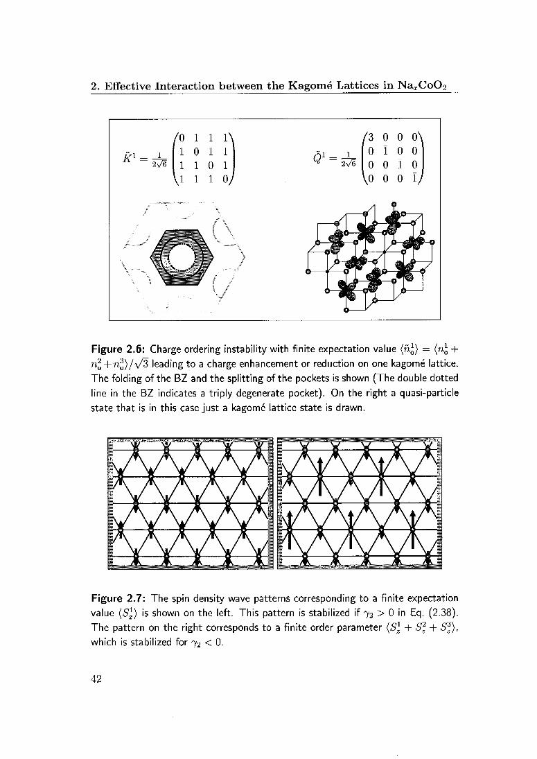
2. Effective Interaction between the Kagomé Lattices in NaxCo02
Kl = -h,
/0 1 1 1\
110 11
2V^ 110 1
V i i o/
ë1- i
2\/6
/3 0 0 0\0 ï 0 0
0 0 ï 0
\o o o ï/
nj +Figure 2.6: Charge ordering instability with finite expectation value (nj)
no + no)/v/3 leading to a charge enhancement or reduction on one kagomé lattice
The folding of the BZ and the splitting of the pockets is shown (The double dotted
line in the BZ indicates a triply degenerate pocket). On the right a quasi-particle
state that is in this case just a kagomé lattice state is drawn.
Figure 2.7: The spin density wave patterns corresponding to a finite expectation
value (S]) is shown on the left. This pattern is stabilized if 72 > 0 in Eq. (2.38).The pattern on the right corresponds to a finite order parameter (Si + S2 + Sf),which is stabilized for 72 < 0.
42
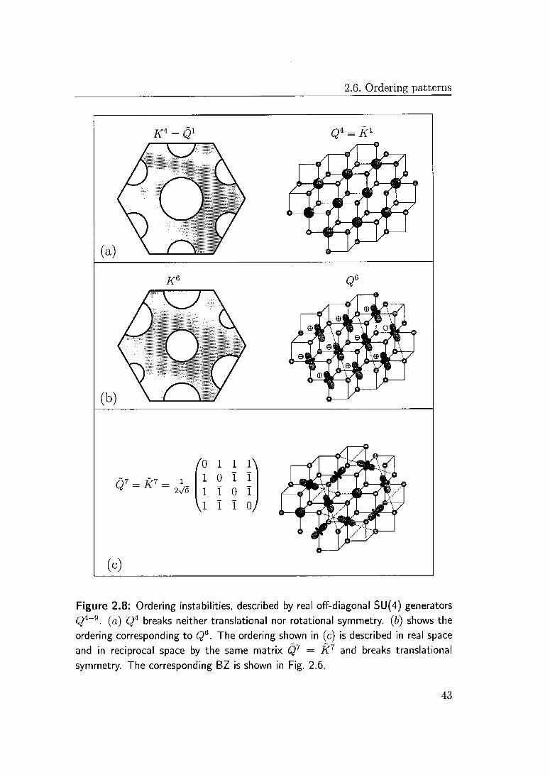
2.6. Ordering patterns
Figure 2.8: Ordering instabilities, described by real off-diagonal SU(4) generators
Q4-9. (a) Q4 breaks neither translational nor rotational symmetry, (b) shows the
ordering corresponding to Q6. The ordering shown in (c) is described in real space
and in reciprocal space by the same matrix Q7 — K7 and breaks translational
symmetry. The corresponding BZ is shown in Fig. 2.6.
43

2. Effective Interaction between the Kagomé Lattices in NaxCoQ2
parallel to [111], i.e., along the c-axis perpendicular to the layer. This
quadrupolar field would be driven by the symmetry reduction discussed
above, through trigonal distortion and direct dd-hopp'mg among the t2g
orbitals.
Spin: While the corresponding order parameter (S4) breaks time reversal
symmetry, space group symmetry is conserved. This order is spatially
uniform analogous to a ferromagnet without, however, having a net mag¬
netic moment. Because the magnetic moment associated with the Fermi
surface pocket at the T point is opposite and three times larger than the
moment at the three M pockets. While the net dipole moment vanishes
on every site, this configuration has a finite quadrupolar spin density cor¬
responding to the onsite spin density distribution of the same form as the
charge distribution in Eq. (2.39), which also belongs to Fi representation
of D3. It is also important to note that no third order terms are allowed
due to broken time reversal symmetry, such that the transition to this
order would be continuous.
r = 5, 6
Charge: The order parameters (n5) = 775 and (n6) — ?76 transform accord¬
ing to the irreducible representation T3 of the cubic point group. The
Landau expansion of the free energy is given by
AF = |(7752 + T72) + §776(3^ - 7762) + 1(VÏ + ri)2, (2.40)
whose global stability requires 7 > 0. The third order term, allowed
here, induces a first order transition and simultaneously introduce an
anisotropy which is not present in the second- and fourth-order terms.
We can write (775, /ye) = r](cosip,smip) and obtain
AF-%2 + ^773sin3^ +j774. (2.41)
Depending on the sign of ß the stable angles will be y — sign(/?)7r/2 -f
2irn/Z. This yields three degenerate states of uniform orbital order whose
charge distribution has the quadrupolar form:
p{r) oc e^ (4^ +^) +w(^ +tt«)-, (2.42)
+^2(V£yVV + %z^y) + C.C.
44

2.6. Ordering patterns
with a tensor operator belonging to T3 of D3. Each state is connected
with the choice of one M pocket which has a different filling compared
to the other two (Fig. 2.8 (b). The main axis of each state points locally
along one of the three cubic body-diagonals, [1,1,1], [1,1,1], [1,1, Ï], and
the sign of the local orbital wave function is staggered along the corre¬
sponding direction on the triangular lattice, [2,1,1], [1, 2,1], [1,1,2]. In
this way the rotational symmetry is broken but the translational symme¬
try is conserved. The matrices Q5 and Q& commute with Q4 such that
the external symmetry reduction has only a small effect on this type of
order.
• Spin: The spin densities (S^) and (Sz ) also belong to the two-dimensional
representation T3 of the cubic point group. Here time reversal symme¬
try ensures that the Landau expansion only allows even orders of the
order parameter (775,776) = 77(cos^,sin^) (i.e., ß = 0 in Eq. (2.40)). The
continuous degeneracy in <p is only lifted by the sixth order term, given
by
ftà + Vif + Ôfit(ZV2 - ni)2 ^ |t76 + 5ff sin2 3^ (2.43)
Stability requires 8\ > max{0, —82}. The anisotropy is lifted by the 82-
term which give rise to two possible sets of three-fold degenerate states.
Depending on the sign of 82 we have a minimum of the free energy for
<p — (1 — sign<52)7r/4 + 7m. The corresponding spin densities have no net
dipole on every site, but again a quadrupolar form of the same symmetry
as for the charge, given by Eq. (2.42).
r = 7,8,9
• Charge: The order parameters (n%) for i — 7, 8, 9 transform irreducibly
under space group symmetries with the representation Fi?. The expan¬
sion (2.38) of the free energy holds also for these order parameters. The
third order term makes the transition first order and favors the symmet¬
ric rotationally invariant combination of the order parameters, described
by the matrix Q7 = (Q7 + Q8 + Q9)/VZ = K7 shown in Fig. 2.8 (c).
The folding of the BZ and the splitting of the bands is the same as in
Fig. 2.6. The orbital pattern of the non-degenerate quasi-particle band is
also shown in Fig. 2.8 (c). It consists of atomic ip° orbitals pointing along
45

2. Effective Interaction between the Kagomé Lattices in NaxCo02
all four cubic space diagonals. Translational but not rotational symmetry
is broken.
• Spin: The discussion for the spin density operators is analogous to the
discussion in the section r = 1,2,3.
r = 10,11,12
• Charge: The order parameters (nl) for i = 10,11,12 transform irreducibly
under space group symmetries with the representation T4. For the T/i
representation of Td, there is no third order invariant. All other terms in
Eq. (2.38) are however also invariants for T^ The absence of the third
order term leads to continuous transition. The stabilized state for a < 0
depends on the sign of 72 in Eq. (2.38).
For 72 > 0 a nontrivial minimum with (n11) = (n12) — 0 exists, which
is described by the hermitian, imaginary matrix Q10. If A is an eigen¬
value of Qw, then —A is also an eigenvalue of Q10 and the corresponding
quasi-particles are connected by time reversal symmetry. Therefore the
non-vanishing eigenvalues of Q10 belong to quasi-particle states, which
are not invariant under time reversal symmetry. They are given by com¬
plex linear combinations of t2g orbitals. For complex linear combinations
of t2g orbitals, the expectation value of the orbital angular momentum
operator (L) does not vanish in general, as can be seen from Table 2.5.
In Fig. 2.9 (a), the pattern of the angular momentum expectation values
(L) for a quasi-particle of Qw is shown. It is invariant under translations
along ax and staggered under translations along a2 and a3. The expec¬
tation values of L are parallel to [Oil]. The folding of the BZ and the
splitting of the bands is shown in Fig. 2.9 (c). Rotational, translational
and time reversal symmetry is broken and the state has the magnetic
point-group 2/m.
For 72 < 0 the symmetric combination Qw = (Q10+Qn+Q12)/\/Z = Kwis stabilized. The angular momentum pattern for a quasi-particle with
non-vanishing eigenvalue is shown in Fig. 2.9 (a). Depending on the site,
the expectation value points along [100], [010], [001] or [III] and the
magnitudes are such, that the pattern is rotationally invariant and the
expectation value of the total angular momentum perpendicular to the
46

2.6. Ordering patterns
Figure 2.9: Transitions to time reversal symmetry breaking states, where the
expectation value of the orbital angular momentum (L) on the Co-sites is finite.
(a) States where the angular momentum does not lie in the plane. Kw — Q10. (b)States with the angular momentum in the plane. K13 —
—Q13. (c) The folding
of the BZ and the hybridization of the bands for (a). Dotted lines indicate double
degenerate bands.
47

2. Effective Interaction between the Kagomé Lattices in Naa;Co02
plane vanishes. The folding of the BZ and the splitting of the pockets is
shown in Fig. 2.9 (c). This state has the magnetic point group 3_m. Note,
that these states can also be considered as a kind of staggered flux states.
The matrices Q10"12 commute with Q4 and therefore the transitions arc
only little affected by a trigonal distortion.
• Spin: The spin density order parameters (Slz) for i = 10,11,12 also trans¬
form under space group symmetries like T^ and except for the spin de¬
pendent quasi-particle energy, the discussion is the same as for the charge
density operators. Note, however, that these spin density operators do
not change sign under time reversal symmetry, because both the orbital
angular momentum and the spin is reversed. This, however does not lead
to a third order term in the Landau expansion, as there is no third order
invariant for the T4 representation anyway.
r = 13,14,15
• Charge: The order parameters (ri1) for i = 13,14,15 transform irreducibly
under space group symmetries with the representation T£. The matrices
Q13-15 are a|go imaginary and time reversal symmetry changes the sign of
the order parameters. The Landau expansion of the free energy is given
as above by Eq. (2.38) with ß = 0.
For 72 > 0 and a < 0 a minimum of the free energy is given by the order
parameter (n13). The angular momentum pattern of the quasi-particles is
shown in Fig. 2.9 (b). The expectation values of L lie in the Co02-plane
and arc parallel to the ai direction. Their sign is staggered along the a2
and a3 direction. The quasi-particles consist of states belonging to the T
and the M pocket. The folding of the BZ is given in Fig. 2.9 (c), but with
the single dotted line in the center being a doubly degenerate M pocket.
Rotational, translational and time reversal symmetry is broken.
For 72 < 0 the symmetric combination Q13 ~ (Q13 + Qu + Q15)/V^ -—K13 is stabilized. The pattern of the quasi-particles corresponding to
Q13 is shown in Fig. 2.9 (b). It consists of non-magnetic sites with a <po
orbital perpendicular to the plane and of sites with angular momentum
expectation values along a;. Rotational symmetry is not broken in this
case. The folding of the BZ and the splitting of the bands is shown in
Fig. 2.9 (c). All angular momentum expectation values for these two
48

2.7. Possible instabilities
states lie in the Co02-plane. Therefore, it is not possible to interpret
these states as staggered flux states.
• Spin: The spin density order parameters (Slz) for i — 13,14,15 are in¬
variant under time reversal symmetry. Therefore, the third order term in
Eq. (2.38) is allowed and the transition is a first order transition.
An overview over the different symmetry breaking states is provided in Ta¬
ble 2.6.
2.7 Possible instabilities
2.7.1 Coupling constants
As can be seen from Table 2.4, the coupling constants for the spin density
wave (SDW) transitions As are rather negative whereas the charge coupling
constants Ac tend to be positive. This is not surprising as only local repulsive
interaction is considered here, that tends to spread out the charge as much as
possible.
The coupling constants Ar with r — 0,..., 3 depend on the intra-orbital
Coulomb repulsion U. As U is the largest Coulomb integral, the absolute
value of these coupling constants is biggest. The remaining coupling constants
Ars do not depend on U. For J' — 0 they are also independent of r. For
finite J' the degeneracy between the real (4-9) and imaginary (10-15) SU(4)
generators is lifted. In order to compare the different coupling constants, we
reduce the number of parameters and we use the relations U = U' + 2JH and
Jh = J', that hold exactly in a spherically symmetric system, but can be
assumed to hold approximately for our system. The ratio a — U'/U is positive
and usually larger than 1/2 and smaller than 1. These assumptions allow
to order the dimensionless coupling constants AC//s — 9AC^S/(2U) according to
their strength. In Fig. 2.10 the dimensionless coupling constants Ar arc shown
as functions of a. The most negative coupling constant is the ferromagnetic
one with Ag —
—6 + 3a. For a close to 1, the coupling constant for spin
density order A\ — —(2 + a) is comparable. Smaller but still clearly negative
are also the coupling constants for the spin density angular momentum states
Aj0 — — (1 + a). The coupling constants A4 — A| — 1 — 3a are also negative.
Finally, the coupling constant for time reversal symmetry breaking angular
momentum states Ac10 ~ 3 — 5a and for the charge density order A^ = 4 — 5a
49
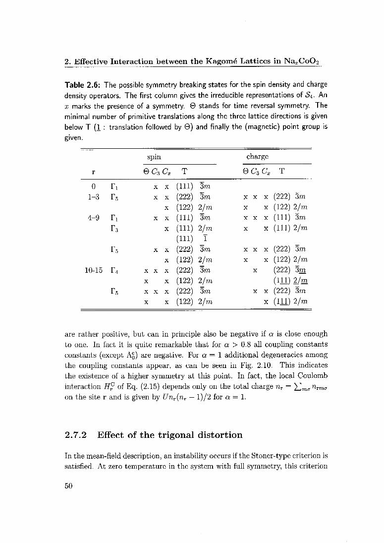
2. Effective Interaction between the Kagomé Lattices in Na.j;Co02
Table 2.6: The possible symmetry breaking states for the spin density and charge
density operators. The first column gives the irreducible representations of S4. An
x marks the presence of a symmetry. 0 stands for time reversal symmetry. The
minimal number of primitive translations along the three lattice directions is given
below T (1 : translation followed by ©) and finally the (magnetic) point group is
given.
spin charge
ec3cx t ecscx t
0 Ti X X (111' 3m
1-3 r5 X X (222; 3m X X X (222) 3m
X (122; 2/m X X (122) 2/m4-9 Ti X X (111; 3m X X X (111) 3m
r3 X (111;
(111)
2/mT
X X (111) 2/m
r5 X X (222) 3m, X X X (222) 3m
X (122) 2/m X X (122) 2/m10-15 r4 X X X (222) 3m X (222) 3m
X X (122) 2/m (111) 2/m
r5 X X X (222) 3m X X (222) 3m
X X (122) 2/m X (111) 2/m
are rather positive, but can in principle also be negative if a is close enough
to one. In fact it is quite remarkable that for a > 0.8 all coupling constants
constants (except Aq) are negative. For a — 1 additional degeneracies among
the coupling constants appear, as can be seen in Fig. 2.10. This indicates
the existence of a higher symmetry at this point. In fact, the local Coulomb
interaction H^ of Eq. (2.15) depends only on the total charge nr — J2manrmaon the site r and is given by Unr(nT — l)/2 for a — 1.
2.7.2 Effect of the trigonal distortion
In the mean-field description, an instability occurs if the Stoner-type criterion is
satisfied. At zero temperature in the system with full symmetry, this criterion
50

2.7. Possible instabilities
a=0.5 <x=1.0
Figure 2.10: The dimensionless coupling constants Ar = 9Ac/sV/(2f/) as func¬
tions of a — U'/U. The relations U — £/' + 2Jh and J' — Jr- are assumed to hold.
The solid (dashed) lines denote the charge (spin) coupling constants.
reads in our notation as
-Ar75D(EF) = 1, (2.44)
where D(EF) is the density of states per spin and per hole pocket. For rather
small pockets D(EF) is given by \/Z/(2iit) « 0.28/t in our tight-binding model,
increases however with decreasing EF (cf. Fig. 2.5). From Eq. (2.44) we can
estimate that the critical U must be larger than 101 for having a ferromagnetic
instability. With the introduction of the trigonal distortion, as it was discussed
in Sec. 2.5, the Stoner criteria of Eq. (2.44) are modified.
For the order parameters described by the matrices üf°, KA, K5~6, and
AT10-12, that commute with the trigonal distortion, K4, the change of the Stoner
criterion is only due to the changing of the density of states at the M and the
F pockets by the trigonal distortion, and the Stoner criterion is only slightly
modified as long as all four pockets exist. On the other hand, the instabilities
towards states, where the order parameters with the matrices K13~15 are finite,
51
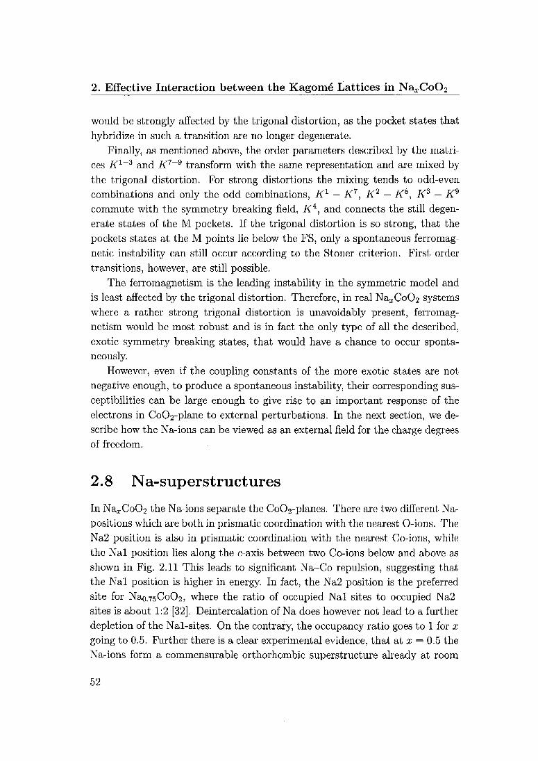
2. Effective Interaction between the Kagomé Lattices in Na2;Co02
would be strongly affected by the trigonal distortion, as the pocket states that
hybridize in such a transition are no longer degenerate.
Finally, as mentioned above, the order parameters described by the matri¬
ces A'1-3 and K7~9 transform with the same representation and are mixed by
the trigonal distortion. For strong distortions the mixing tends to odd-even
combinations and only the odd combinations, K1 — K7, K2 — K8, K3 — K9
commute with the symmetry breaking field, K4, and connects the still degen¬
erate states of the M pockets. If the trigonal distortion is so strong, that the
pockets states at the M points lie below the FS, only a spontaneous ferromag¬
netic instability can still occur according to the Stoner criterion. First order
transitions, however, are still possible.
The ferromagnetism is the leading instability in the symmetric model and
is least affected by the trigonal distortion. Therefore, in real Na.i;Co02 systems
where a rather strong trigonal distortion is unavoidably present, ferromag¬
netism would be most robust and is in fact the only type of all the described,
exotic symmetry breaking states, that would have a chance to occur sponta¬
neously.
However, even if the coupling constants of the more exotic states are not
negative enough, to produce a spontaneous instability, their corresponding sus¬
ceptibilities can be large enough to give rise to an important response of the
electrons in Co02-plane to external perturbations. In the next section, we de¬
scribe how the Na-ions can be viewed as an external field for the charge degreesof freedom.
2.8 Na-superstructures
In NaxCo02 the Na-ions separate the Co02-planes. There are two different Na-
positions which arc both in prismatic coordination with the nearest O-ions. The
Na2 position is also in prismatic coordination with the nearest Co-ions, while
the Nal position lies along the c-axis between two Co-ions below and above as
shown in Fig. 2.11 This leads to significant Na-Co repulsion, suggesting that
the Nal position is higher in energy. In fact, the Na2 position is the preferredsite for Na0.75CoO2, where the ratio of occupied Nal-sites to occupied Na2-
sites is about 1:2 [32]. Deintercalation of Na does however not lead to a further
depletion of the Nal-sites. On the contrary, the occupancy ratio goes to 1 for x
going to 0.5. Further there is a clear experimental evidence, that at x — 0.5 the
Na-ions form a commensurable orthorhombic superstructure already at room
52

2.8. Na-superstructures
Figure 2.11: The two different Na-positions in Na;rCo02. Note, that the Nal
position is located between two Co-ions along the c-axis.
temperature [28]. For several other values of x also superstructure formation
has been reported, but x — 0.5 shows the strongest signals and has the simplest
superstructure [29, 30]. In addition for x — 0.5 samples a sharp increase of the
resistivity at 50K respectively at 30K was reported [27, 31, 41],This experimental situation is rather surprising. Naively, one expects com¬
mensurability effects to be strongest at x — 1/3 or at x = 2/3 on a triangular
lattice but not at x = 0.5. Therefore, it was concluded that structural and
electronic degrees of freedom are coupled in a subtle manner in Naj;Co02 [32].In this section we show how the different ordering patterns can couple to
the observed Na-superstructure at x — 0.5. Before going into the details,
we note that due to our starting point of inter-penetrating kagomé lattices,
commensurability effects will be strongest for samples where the Na-ions can
form a simple periodic superstructures that double or quadruple the area of the
unit cell, since specifying a single kagomé lattice also quadruples the unit cell.
For x = 0.5 such simple superstructures exist as shown in Fig. 2.12. A sodium
superstructure couples to the charge but not to the spin degrees of freedom in
the Co02-layer. In our model, there are 15 collective charge degrees of freedom.
From Fig. 2.10 can be seen that A£ is most negative for r = 4,... ,9. Hence,
these modes are the "softest" charge modes generating the strongest response to
a Na-pattern. As shown in Fig. 2.8, the charge order corresponding to r — 4, 5, 6
does not enlarge the unit cell and does therefore not optimally couple to the Na-
53

2. Effective Interaction between the Kagomé Lattices in NaxCo02
H Na(z=l/4) O Co(z=l/2) o Na (z=3/4)
Figure 2.12: Two different Na-superstructures in Nai/2Co02. The left one does
not break rotational symmetry and would drive a charge ordering as shown in
Fig. 2.8 (c). The right one is in fact realized in Nai/2Co02, it is obtained from
the right one by shifting the Na-chains along the arrows. This shift is due to the
Coulomb repulsion of the Na-ions. z denotes the position along the c-axis.
Figure 2.13: The right hand side shows the charge ordering pattern corresponding
to the matrix Kl — K7, which consists of alternating rows of dx and dy — dz
orbitals. On the left hand side the original BZ, the orthorhombic BZ due to the
charge ordering and the experimentally observed reduced orthorhombic BZ (dark)are shown.
54

2.8. Na-superstructures
patterns that can be formed with x — 0.5. However the orbital pattern shown in
Fig. 2.8 (c) has lobes of electron density pointing towards selected Nal and Na2
positions. For x — 0.5 it is possible to occupy all these and only these positions.
This leads to the left Na-superstructure of Fig. 2.12. In other words, this Na-
superstructure couples in an optimal way to this rotationally symmetric charge
pattern. Further, the Landau expansion shows that the rotationally symmetric
combination is favored by the third-order term. Therefore, it is clear that the
electronic degrees of freedom would favor this Na-superstructure. This pattern
however does not maximize the Na-ions distances. It is apparent that the
average distances between the Na-ions can be increased, if every second of the
one-dimensional sodium chains is shifted by one lattice constant as shown in
Fig. 2.12. In this way an orthorhombic Na-superstructure is obtained, which
is the one observed in experiments [29]. This orthorhombic pattern does not
drive the rotationally symmetric charge pattern shown in Fig. 2.8 (c), which
is described by the matrix K7 = (K7 + K8 + K9)/\/3. It might however
drive the orthorhombic charge pattern described by the matrix K7 or rather
the orthorhombic charge pattern described by Kl — K1', as in the presence of
trigonal distortion the Kl and K7 mix and the odd combination will have the
most negative coupling constant. This charge pattern is shown in Fig. 2.13. It
consists of lines of dx orbitals alternating with lines of the linear combination
dy — dz orbitals. Note, that this charge pattern corresponds to the mixed
K1 — K7 matrix, the charge is not uniformly distributed on the Co-atoms. In
this charge pattern, the Nal-sites above the (dy — dz) Co-sites will be lower in
energy than the Nal-sites above the dx Co-sites and similarly the Na2-positions
are separated into nonequivalent rows.
In reciprocal space, such a charge ordering leads to a folding of the BZ
such that the two M pockets hybridize. The ordering of the Na-ions along
the chains leads to a further folding of the BZ and to a hybridization of the
bands, as it is shown in Fig. 2.13. The schematic FS in Fig. 2.13 is drawn to
illustrate the hybridization occurring due to the translational symmetry break¬
ing. Li et al. performed density-functional calculations in order to determine
the band-structure of Nao.sCo02 in the presence of the orthorhombic super¬
structure from first-principles [74]. Quite generally one can assume that this
superstructure, which specifies a direction on the triangular lattice, can lead
to quasi-onedimensional bands in the reduced BZ. For such one-dimensional
bands, nesting features are likely to occur and would lead to a SDW-like in¬
stability, as it was observed at 53 K by Huang et al. [28, 55]. Such a transition
55

2. Effective Interaction between the Kagomé Lattices in Na:rCo02
could open a gap at least on parts of the FS and in this way lead to the drastic
increase of the resistivity observed at 53 K [27]. At higher temperature, the re¬
sistivity is comparable in magnitude to the metallic samples and increases only
slightly with lowering temperature. This weakly insulating behavior could be
another effect of Na-ion ordering. Since the rotational symmetry is broken,
domains can be formed. The existence of domain walls would be an obsta¬
cle for transport where thermally activated tunneling processes play a role. It
would be interesting to test this idea by removing the domains and see whether
metallic temperature dependence of the resistivity would result. A bias on the
domains can be given by in-plane uniaxial distortion.
To finish this section, we will discuss a further mechanism, that could lead
to a non-magnetic low-temperature instability in Nao.5Co02. In Sec. 2.6 we saw
that the third order term in the Landau expansion, Eq. (2.38), favors always a
rotationally symmetric charge ordering where all three order parameters 771, r]2,
and n3 have the same magnitude. But as argued above, the Na-ion repulsion
leads nevertheless to an orthorhombic charge ordering, where only one order
parameter 771 is finite. From Eq. (2.38), we obtain a Landau expansion for the
remaining two order parameters r}2 and 773 containing only second and forth
order terms. The second order term is given by
^(vl + vD + ßmVs, (2-45)
where
à = a + (71 + y) i}\ and ß = ßrji. (2.46)
The condition for a second order phase transition, that leads to finite values of
772 and 773 is â < \ß\. As we have a > 0 and linear growth of \ß\ and quadratic
growth of à — a with 771, the condition is fulfilled neither for large nor for
small values of 771. But for intermediate values of 771 it can be fulfilled. This
tendency back towards the original hexagonal symmetry in this or a similar
form could be responsible for the appearance of additional Bragg peaks at the
intermediate temperature of 80-100 K in Nao,5Co02 [28], Note however, that
it was speculated that these Bragg peaks only exist over a narrow range of
temperature.
56

2.9. Wannier functions
2.9 Wannier functions
It would be desirable to have an understanding of the localized degrees of free¬
dom in our model. This is usually achieved in a single-band model by calcu¬
lating the Wannier orbitals. However before calculating the Wannier orbitals,
let us introduce first a different set of local states that have a certain relation
to the four kagomé lattices by
<:=7=Ee_iKR<- (2-47)
From Eq. (2.7) follows together with a little algebra that these states are given
by
< --4E E7»'-»+*+- a£w (2-48)V3~i-
R' m
with
N^B -\ln,m if l = m= 1,2,3,(2-49)
_
6 cos[f(r + 5 + l)]-cos[f(r + s+l)]7R'm "
(2tt)2 (r_2s + I)(2r~-S-±)' [Z-M)
where we have written r in the form r — 2(ram+1 + sam_i).d Further, we have
the Parseval relation Yln |-^R,m|2 — 1 for the amplitudes. The amplitudes iR+ai
decay fast but not exponentially fast. The moduli squared of these local wave
functions slightly above and below the Co02-plane are shown in Fig. 2.14. The
white lines correspond to Co sites. The thick white line marks the central Co
site. The Na positions are above (below) the triangles with smaller amplitudes
(cf. Fig. 2.3). Note, that the kagomé lattice with / — 0 has the origin in the
center of a hexagon and therefore the corresponding local orbital is symmetric
with respect to 27r/3 rotations around the c-axis.
Now, we go back to the definition of the Wannier orbitals. Our first guess
would be
< = <+a(,„ = ^Ee-^+^-^C = ^E e-iK-(R+ai)«L- (2.51)
dThe index I = 0,1,2,3 takes four values. The index m = 1,2,3 takes only three values
and is cyclic, e.g., m — 1 = 3 for m = 1.
57
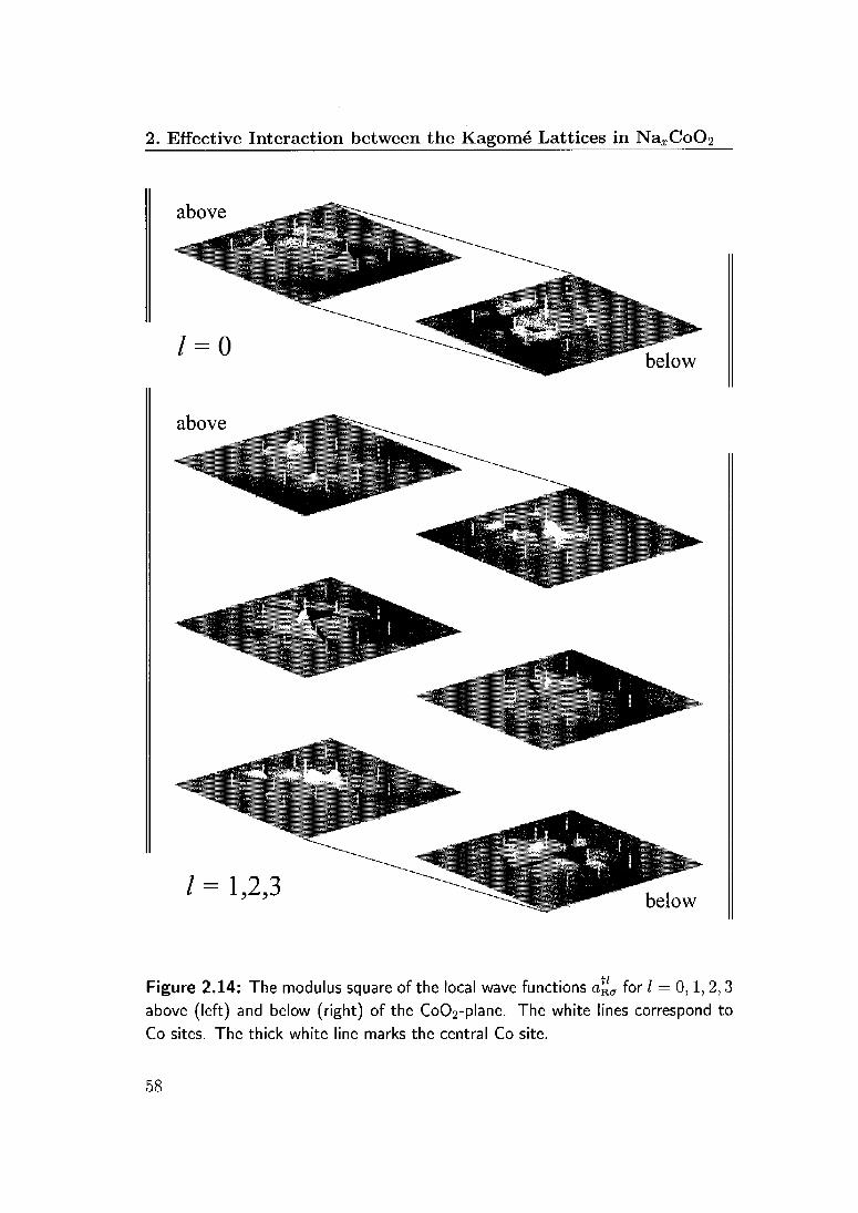
2. Effective Interaction between the Kagomé Lattices in Na.j;Co02
above
below
above
ilSÉHIli
jill|HM|ti. -"fe
/ = 1,2,3MM
below
Figure 2.14: The modulus square of the local wave functions a^ for / — 0,1,2,3
above (left) and below (right) of the Co02-plane. The white lines correspond to
Co sites. The thick white line marks the central Co site.
58

2.10. Superconductivity
For / — 0 we find exactly the orbital a^ shown in the first row of Fig. 2.14. For
I = 1, 2, 3 we find the same orbital shifted by the vector a*. The operators w\adefined in (2.51) generate in fact states that are localized at the site r and have
the full point group symmetry. But are the operators wla the only operators
with these two properties?
In fact it turns out that we have to be careful. In the definition (2.51)we could also have used different phases for the different Bloch states. As in
our approximation the periodic function of the Bloch states does not depend
on k, we can assume that also the phase of the Bloch states entering into the
definition of the Wannier orbitals does not depend on k. On the other hand
the phase could well depend on the pocket index j. If we would for example
shift the phase of all Bloch states with j = 0 in (2.51) by ir, we would obtain
different Wannier orbitals. The Wannier orbitals on the kagomc lattice with
/ = 0 lattice for example would be given by (aRa — aRa — aL — aRa-)/2 instead
of a^a- There is no argument that would allow us to discard one of these
Wannier orbitals as both of them arc invariant under rotations and both do
not decay exponentially. In fact we can see that it is not possible to present
a unique local wave function for a given lattice site that decays exponentially,
but, we can provide four orthogonal local states per enlarged unit cell that
decay algebraically. For the site r these are exactly the states crKa shown in
Fig. 2.14. Which linear combinations of these states has to be used in solving
a local physical problem can not be answered in a general way.
2.10 Superconductivity
So far, the focus in this chapter was on the possible charge and spin density
wave instabilities in NaxCo02- The effective interaction (2.29) is written in
a form that allows to read off directly the coupling constants for the charge
and spin density wave instabilities. Furthermore, this interaction was derived
for values of x close to one, where no superconductivity can be observed in
experiments.
It is, however, instructive to decouple the interaction (2.22) into the different
superconducting channels. To this end, let us define the order parameters
A-' - ^ EEQij(<y~^)- (2-52)K ij
As the effective interaction does not depend on k, we must have singlet pairing
59

2. Effective Interaction between the Kagomé Lattices in NaxCo02
Table 2.7: The coefficients Tsr (singlet) and Tj: (triplet).
rr r
0
1-3
4-9
10-15
^(3U + 16U' + 16Jn + 70J')
^(3C/ + 16C// + 16JH-2J/)
f(Ju + U')0
0
0
0
-U')
for r = 0,..., 9 and triplet pairing for r — 10,..., 15 because the corresponding
matrices Q\j are even respectively odd under the exchange of the indices i and
j. The coupling constants for these superconducting instabilities are given by
r* = Y,(Ami-3Aw)QiiQrjk (2-53)ijkl
ijkl
and tabulated in Table 2.7. Note, that all coupling constants for singlet pairing
are clearly repulsive. The coupling constants for the triplet instability is only
attractive for Jn > U which is usually not the case. Note that only the insta¬
bilities with r — 0 and with r — 4,..., 6 occur in the usual Cooper channel.
The remaining instabilities are given by Cooper pairs with a finite momentum,
similar to a Fulde-Ferrell-Larkin-Ovchinnikov state. These states also break
translational symmetries and depending on their combination also rotational
symmetries. Note, that the degeneracies of the pairing partners for the usual
type of Cooper pairing is guaranteed by inversion symmetry, whereas for the
Fulde-Ferrell type of instabilities, the degeneracy of the states that have to be
paired up is a property of our tight-binding model, that will be at least par¬
tially broken by additional hopping terms or by trigonal distortion. However,
as long as the pockets around the M points are spherical, the degeneracy of the
pairing states for the triplet states with r — 10,..., 12, that only pairs states
belonging to these M pockets, is still guaranteed. In this subsection we do not
attempt to provide a complete discussion of the superconducting instabilities in
our model or even in the hydrated Na;rCo02. For such a discussion it would be
necessary to include charge, spin, and orbital fluctuations in the interactions.
60

2.11. Discussion and conclusion
This could be done using RPA or the FLEX method e We refer to Ref. [70]for a FLEX discussion of superconductivity in Na^Co02. In this work, spin
triplet superconductivity is found, that exists due to the presence of small hole
pockets. However, this triplet superconductor is neither a Fulde-Ferrell state,
nor are the pockets around the M points.
2.11 Discussion and conclusion
In this chapter the properties of a high-symmetry multi-orbital model for the
Co02-layer in combination with local Coulomb interaction are discussed. The
tight-binding model is a zeroth order approximation to the kinetic energy, as it
only includes the most relevant hopping processes using Co-0 7r-hybridization.
Nevertheless it produces the hole pocket with predominantly Oi5 character
around the T point, in agreement with both LDA calculations and ARPES
experiments. Furthermore, the three further pockets around the M points,
although not seen in ARPES experiments, suggest that additional degrees of
freedom that can not be captured in a single-band picture could be relevant.
The existence of identical hole, pockets in the BZ does however not produce
pronounced nesting features.
The local Coulomb repulsion of the t2g orbitals can be taken into account
by an effective interaction of fermions with four different flavors, associated
with the four hole pockets or the four inter-penetrating kagomé lattices. This
effective interaction has a large discrete symmetry group, that allows to classify
the spin- and charge-density operators, and to the determine for every mode
the corresponding coupling constant.
It turns out that with an effective trigonal distortion, that splits the degen¬
eracy between the F and the M points, general corrections to the quadratic part
of the Hamiltonian, such as trigonal distortion or additional hopping terms, can
be taken into account, provided they are small. This effective trigonal distor¬
tion reduces the symmetry of the Hamiltonian down to the space-group sym¬
metries of the Co02-plane, by breaking the gauge symmetries of the effective
interaction.
Most coupling constants are negative for reasonable assumptions on the
Coulomb integrals U, U', J', and JH> but the ferromagnetic coupling constant
is most negative and constitutes the dominant correlation. The charge and
eRPA=Random Phase Approximation, FLEX=FLuctuation-EXchange approximation.
61

2. Effective Interaction between the Kagomé Lattices in NaxCo02
spin density wave instabilities without trigonal distortion are easily described
in a mean-field picture. In reciprocal space the degenerate bands split, and if
bands belonging to different pockets hybridize, the BZ is folded. In real space
different types of orderings are possible. The occupancy of the different t2gorbitals on different sites can be nonuniform, resulting in a charge ordering
with nonuniform charge distribution on the Co-sites. Further, certain real
or complex linear combinations of t2g orbitals can be preferably occupied on
certain sites. In this case, the charge is uniformly distributed on the sites,
but depending on the linear combinations of the orbitals, certain space group
symmetries are broken. The complex linear combinations of t2g orbitals have
in general a non-vanishing expectation value of the orbital angular momentum.
The tendency to these rather exotic states turns out to be smaller than
the ferromagnetic tendency, and this dominance of the ferromagnetic state is
even more enhanced by the trigonal distortion. This is in good agreement with
experiments, where ferromagnetic inplane fluctuations have been observed by
neutron scattering measurements in Na0.75CoO2 [44, 45]. There are also several
reports of a phase transition in Na0.75CoO2 at 22 K to a static magnetic order,
which is probably ferromagnetic inplane but antiferromagnetic along the c-axis
[47, 49, 50].
In Na0.5CoO2, a periodic Na-superstructure couples directly to a charge
pattern in our model and crystallizes already at room temperature, whereas
simple \/3 x ^-superstructures, that would correspond x — 1/3 on- 2/3do not couple.
For general values of x the disordered Na-ions provide a random potential
that couples to the charge degrees of freedom. Due to the incommensurability,
this does not lead to long range order, but the short range correlations will
also be influenced by the charge degrees of freedom in the Co02~layers. This
interaction between the Na-correlations and the charge degrees of freedom could
be the origin of the charge ordering phenomena at room temperature and the
observation of inequivalent Co-sites in NMR experiments [34, 35].
The overall agreement of our model with the experimental situation is good.
Ferromagnetic fluctuations are dominant in our model and in experiments.
Furthermore, our model is based on a metallic state and allows for charge
ordering and spin density ordering transitions without changing the metallic
character of the state. Finally, the clear Na-superstructures, that were found
at x = 0.5, can be understood quite naturally in this model.
On the other hand there are still many open questions for the cobaltates.
62

2.11. Discussion and conclusion
Mainly the origin and the symmetry of the superconducting state of Naa;Co02-yH20
is still under debate. Unfortunately the Na content x — 0.35 is beyond the va¬
lidity of the approximations made in the derivation of our model. But also the
samples with x > 0.5 have still many intriguing properties like the strongly
anisotropic magnetic susceptibility, which shows the unusual Curie-Weiss tem¬
perature dependence. A possible description of the anisotropy of the magnetic
susceptibility could be achieved by introducing a spin-orbit term into the ki¬
netic energy.
63

Seite Leer /Blank leaf
Chapter 3
Bond Order Wave Instabilities
in Doped Frustrated Antiferro¬
magnets: Valence Bond Solids
at Fractional Filling
3.1 Introduction
Highly frustrated quantum magnets are fascinating and complex systems where
the macroscopic ground-state degeneracy at the classical level leads to many in¬
triguing phenomena at the quantum level. The ground-state properties of spinS — 1/2 Heisenberg antiferromagnets on the kagomé and the pyrochlore lattice
remain still puzzling and controversial in many aspects. While the magnetic
properties of the Heisenberg and extended models have indeed been studied
for quite some time, the investigation of highly frustrated magnets upon dop¬
ing with mobile charge carriers has started recently [86-90]. Such interest has
been motivated for example by the observation that in some strongly corre¬
lated materials, such as the spinel compound LiV204, itinerant charge carriers
and frustrated magnetic fluctuations interact strongly [91, 92]. Furthermore,the possibility of creating optical kagomé lattices in the context of cold atomic
gases has been pointed out [93], making it possible to "simulate" interactingfermionic or bosonic models in an artificial setting [94].
At this point we should stress that the behavior in a simple single-bandmodel at weak and at strong correlations are not expected to be related in a
65
3. Bond Order Wave Instabilities in Doped Frustrated AF
trivial way. The weak-coupling limit allows us to discuss the electronic proper¬
ties within the picture of itinerant electrons in momentum space based on the
notions of a Fermi surface and Fermi surface instabilities (see, e.g., Refs. [86]and [89]). Considering for example the Fermi surfaces of a triangular or a
kagomé lattice at half-filling we do not find any obvious signature of the mag¬
netic frustration present at large U. Although at weak coupling these systems
do not seem to be particularly special, at intermediate to strong coupling the
high density of low-energy fluctuations of the highly frustrated systems dis¬
plays characteristic features from which the physics of the frustrated system of
localized degrees of freedom will emerge [87, 88].In the following we study a class of highly frustrated lattices, the so-called
bisimplex lattices [95], which are composed of corner-sharing simplices residing
on a bipartite underlying lattice. We restrict ourselves to the triangle and
the tetrahedron as the basic building blocks in the following. This class hosts
lattices such as the kagomé or the pyrochlore lattice and their lower-dimensional
analogues, the kagomé strip and the checkerboard lattice (cf. Fig. 3.1).Our main result is the spontaneous symmetry breaking taking place at a the
electron density of one electron per simplex (n — 2/3 for the kagomé lattice and
the kagomé strip, n — 1/2 for the pyrochlore and the checkerboard lattice) for
a wide range of interactions. This instability is driven by a cooperative effect
of the kinetic energy and the nearest-neighbor (nn) interaction, which can be
an antiferromagnetic exchange interaction and/or nearest-neighbor Coulomb
repulsion. In the resulting low-symmetry phase only lattice symmetries are
broken,a resulting in different bond strengths, e.g., different expectation values
of the kinetic energy on equivalent lattice bonds. Therefore, we will refer to
this instability in the following as a bond order wave (BOW) instability. An
alternative name would be Peierls or spin Peierls instability, however, these
terms could be misleading as contrary to the original Peierls transition the
elasticity of the lattice is not relevant in our model, i.e., the BOW instability
can also occur in an infinitely rigid lattice and, in contrast to the spin Peierls
transition, the kinetic energy and the charge degrees of freedom play a crucial
role for the BOW instability described in the chapter.
The outline of this chapter is as follows. In a first section we introduce the
lattices and the model. The limit of decoupled simplices, which we study in
Sec. 3.3 by the analysis of the spectrum of isolated or weakly coupled simplices,
aIn the kagomé and in the pyrochlore lattice the inversion symmetry is broken, whereas
in the lower-dimensional analogues a doubling of the elementary unit cell occurs.
66
3.2. Model and lattices
provides an illuminating starting point. An additional intuitive and somewhat
complementary picture of the spontaneous symmetry breaking can be obtained
from a simple doped quantum dimer model, that we discuss in Sec. 3.4. For the
isotropic t-J model on kagomé and on the pyrochlore lattice we show in Sec. 3.5,
that within the Gutzwillcr mean-field formalism the BOW instability is clearly
dominant at the considered filling. Without interactions, the bisimplex lattices
with one electron per simplex have half-filled particle-hole symmetric bands,
with empty flat bands on top of them. The half-filled bands arc exactly the
bands of the underlying bipartite lattices and the empty bands can be ignored
in the weak-coupling limit. Based on these facts we derive in Sec. 3.6 effective
models for the underlying bipartite lattices in weak-coupling. These models we
analyze with rcnormalization group (RG) and/or within mean-field methods.
Also in weak-coupling we can establish the presence of the BOW phases for
the kagomé strip and the checkerboard lattice. In Sec. 3.7 we compare the
results of the previous sections to extensive numerical data that corroborate
the theoretical picture. Before we summarize and conclude in Sec. 3.9 we focus
in Sec. 3.8 on the Dirac points that form the Fermi surface for the kagomé
lattice at the considered filling. An analysis of the wave function of the non-
interacting (tight-binding) states close to these points helps to understand the
observed symmetry breaking. We also discuss some additional peculiarities
of these states and compare to the analogous phenomena for the honeycomb
lattice. The major part of the results presented in this chapter is published in
the references [96] and [97]. The numerical calculations (Sec. 3.3.1 and Sec. 3.7)were performed by Andreas Läuchli and Sylvain Capponi in the framework of
a collaboration on Ref. [96], The reference [97] contains additional numerical
results for the checkerboard lattice that are not presented in this thesis.
3.2 Model and lattices
We study in this chapter the Hamiltonian H — H0 + Hmt on the bisimplex
lattices shown in Fig. 3.1 at the filling of two electrons per simplex. The
kinetic part is given by
(ij) <t=U
67
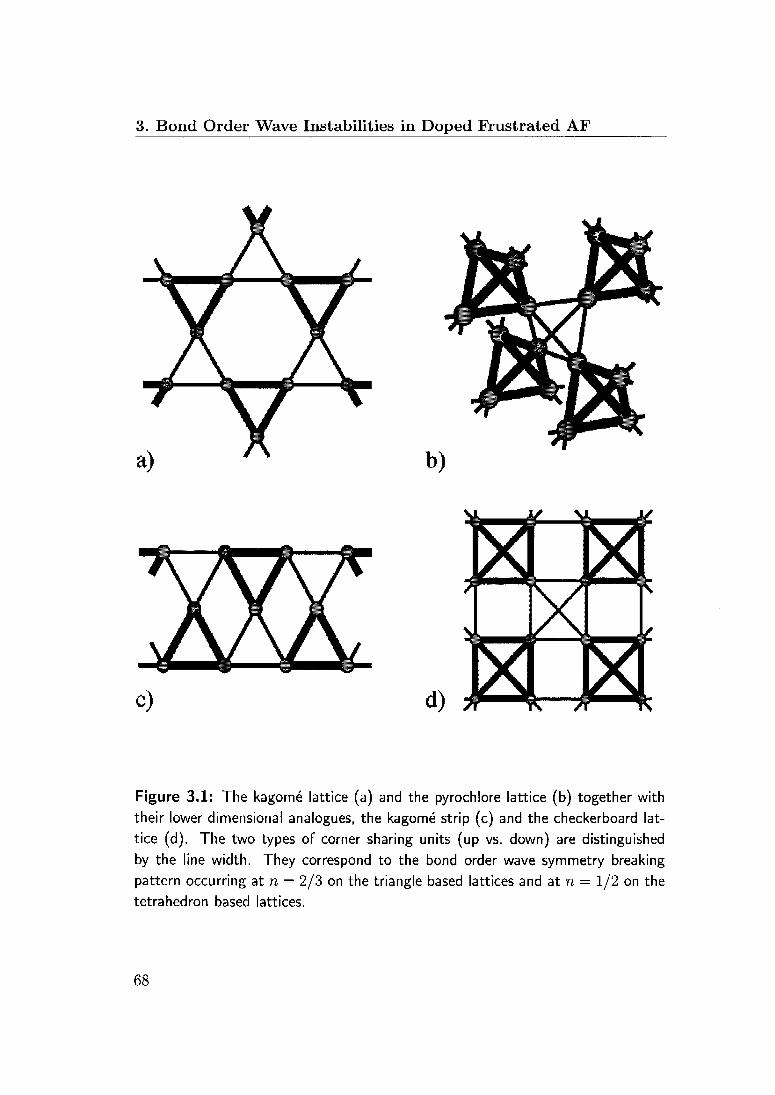
3. Bond Order Wave Instabilities in Doped Frustrated AF
Figure 3.1: The kagomé lattice (a) and the pyrochlore lattice (b) together with
their lower dimensional analogues, the kagomé strip (c) and the checkerboard lat¬
tice (d). The two types of corner sharing units (up vs. down) are distinguished
by the line width. They correspond to the bond order wave symmetry breaking
pattern occurring at n — 2/3 on the triangle based lattices and at n — 1/2 on the
tetrahedron based lattices.
68
3.3. The limit of decoupled simplices
with the hopping matrix element t. The sum zZuj) runs over a^ DOnds of the
bisimplex lattices. The interaction part of the Hamiltonian is given by
Him = U Y^ n^nü + Jj2si-Si + VY1 UiUi (3l2)i (ij) (ij)
with onsite repulsion U, n.n. repulsion V, and n.n. spin exchange J. For U — oo
we obtain the strong coupling Hamiltonian
HUJ,V = VH0V + jJ2Si-Sj + vY,ntni> (3-3)(ij) (ij)
= H^j + V'^rurij, (3.4)(ij)
where V is the projection operator that enforces the single occupancy constraint
and V — V + J/4. For V — 0 the strong coupling Hamiltonian reduces to the
usual t-J model. The sign of the hopping amplitude t is relevant on these highly
frustrated lattices and in the following discussion it will always be positive. A
negative sign of t will most likely induce ferromagnetic tendencies at the fillings
we are considering [98],The kagomé lattice and the pyrochlore lattice consist of corner-sharing tri¬
angles and tetrahedra, respectively. They are shown in Fig. 3.1 together with
their lower dimensional analogues, the kagomé strip and the checkerboard lat¬
tice. The centers of the triangles in the kagomé lattice form a honeycomb
lattice, whereas the centers of the tetrahedra in the pyrochlore lattice reside
on a diamond lattice. These two underlying lattices and also the underlying
lattices of the kagomé strip and the checkerboard lattice are bipartite and we
can separate the triangles and the tetrahedra into two different classes, which
is visualized in Fig. 3.1 by a different line-style (light and bold bonds). To refer
to triangles (tetrahedra) of a given class we call them up- and down-triangles
(tetrahedra), and the same for the bonds. The considered lattices all have
inversion centers, that map the up-bonds onto down-bonds and vice versa.
3.3 The limit of decoupled simplices
To get a basic understanding of the effect of doping in highly frustrated lattices
we first consider the limit of decoupled units by turning the couplings within
the down-subunits off. Eventually we will connect this limit with the uniformly
69

3. Bond Order Wave Instabilities in Doped Frustrated AF
connected lattice. For this purpose we use the parameter a (0 < a < 1) to
tune the coupling strength of the down-bonds as (at, aJ), while the up-bonds
are constant (t, J) in our Hamiltonian. In this way the inversion symmetry is
explicitly broken. The eigenvalues of Ht.j and their degeneracies are listed in
Table 3.1 for a single triangle and a single tetrahedron. For t > 0 and J > 0,
there is a single state with two electrons, Ne — 2, that has the lowest energy
of all states and, furthermore, is separated from the remaining spectrum by a
finite gap. This state has at the same time the lowest kinetic energy (—2t or
—4t, respectively) of all states and gains the maximal exchange energy (—J)for two spins. This state is not frustrated anymore because it minimizes the
kinetic and the exchange energy at the same time.
After having revealed this particularly stable state with two electrons on
a single unit, we are naturally led to the question whether the homogeneous
lattices could spontaneously exhibit strong and weak units at the filling n —
2/3 for the triangle based lattices and at n — 1/2 for the tetrahedron based
ones. Such an instability has the character of a bond order wave - modulated
expectation values of the bond energies - and yields an insulating fully gapped
ground state. One way to address this question is to track the evolution of
the excitation gaps to all forms of excitations as a function of a. If the gaps
do not close before reaching a — 1 this would suggest an instability towards
spontaneous symmetry breaking.
3.3.1 Approaching the uniform lattices
We now determine these gaps for the kagomé lattice numerically as a function
of the parameter a, which is proportional to the inter-triangle couplings. Our
results are obtained from exact diagonalization (ED) and the contractor renor-
malization (CORE) algorithm [99-102]. This latter method extends the range
of tractable sizes of finite clusters, based on a careful selection of relevant low-
energy degrees of freedom. In order to apply this algorithm, the lattice has to
be divided into blocks; here, we naturally choose the up-triangles. A reduced
Hilbert space is defined by retaining a certain number of low-lying states on
each block. The choice of the states to keep depends also on the quantities to
be obtained. While for a ground-state calculation fewer states already provide
good results, one has to retain usually more states to calculate the excited
states. Here we choose to keep the 4 lowest states in the 3-elcctrons sector, the
7 lowest states with 2 electrons and the 2 lowest states in the 1-electron sector.
70

3.3. The limit of decoupled simplices
Table 3.1: Classification of the eigenstates of the t-J model (3.4) on a triangle
and on a tetrahedron. The degeneracy is given in the form r x (2S + 1), where r
is the dimension of the irreducible representation of <S3, respectively <S4l and S is
the total spin of the state. The asterisk denotes the states retained in the CORE
calculations for the kagomé system, see text.
Triangle Tetrahedron
Ne Energy Degen. Energy Degen.
0 0 1 x 1 0 1 X 1
1 -2t
t
1 x2
2x2
* -Zt
t
1 x 2
3x2
2 -2t-J lxl * -At-J lxl
t-J 2x1 -J 3x1
-t 2x3 * 2t-J 2x1
2t 1x3 -2t 3x3
2t 3x3
3 -3J/2 2x2 * -2t-ZJ/2 3x2
0 1x4 -3J/2 2x2
2t-ZJ/2 3x2
-t 3x4
3* 1x4
4 -3J 2x 1
-23 3x3
0 1 x 5
These states are denoted with an asterisk in Table 3.1. This choice leads to
a reduction of the local triangle basis from 27 down to 13 states, thus allow¬
ing indeed to perform simulations on larger lattices than would be possible by
conventional ED.
Then, by computing the exact low-lying eigenstates of two coupled triangles,we calculate the effective interactions at interaction range two for each value of
a and we neglect longer range terms. Comparison to ED data on the smaller
clusters shows that this approach gives very good results.
71
3. Bond Order Wave Instabilities in Doped Frustrated AF
The basic excitation gaps of interest in the present problem are the spin
gap, the single particle gap and the two particle gap. These are defined as
follows:
As=1 = E(Ne,l)-E(Ne,0), (3.5)
Alp - ~(E(Ne +1,1/2)+ E(Ne-1,1/2))-E(Ne,0), (3.6)
A2p = \(E(Ne + 2,0) + E(Ne- 2,0)) - E(Ne,0), (3.7)
where E(Ne, Sz) denotes the ground-state energy in the sector with A^ electrons
and spin polarization Sz.
We have determined these gaps on kagomé finite size samples at n — 2/3and J/t — 1 containing 18 to 27 sites. Two different versions of samples with
18 and 24 sites have been treated (vl and v2). The results are displayed in
Fig. 3.2. There are two main observations: (1) the gaps do not close for any
a G [0,1], giving first evidence for the proposed symmetry breaking; (2) there is
a strong dependence of the gap curves on the specific sample. Note that there
is no discrepancy between ED and CORE results. The second phenomenon can
be understood from the discretization of the finite size Brillouin zones: indeed,
the measured gaps directly depend on the distance between the closest point
in the Brillouin zone to the corner of the zone, the K-point. The 18,v2 and
the 27 sites samples both contain this specific point and differ only slightly
in the values of the gap. Thus supporting the claim of a finite gap for all
a G [0,1]. The strong dependence is at the same time also a hint towards a
sizable dispersion of the excitations in this system.
3.4 Doped quantum dimer model
In the previous sections we discussed mostly the case a < 1, where the Hamil¬
tonian itself is not invariant under inversion symmetry. In this case it is natural
to apply a method which is based on the existence of strong subunits (trian¬
gles or tetrahedra) that are only weakly coupled. If the system has in fact the
tendency to develop such strong subunits, the results of this method can be
quantitatively good even for the uniform case. However, in order to get some
insight into the mechanism of spontaneous symmetry breaking, it is desirable
to treat up- and down-triangles (tetrahedra) on an equal footing. In the follow¬
ing, we present a simple but illustrative picture of the mechanism that leads to
the spontaneous breaking of the inversion symmetry.
72

3.4. Doped quantum dimer model
N=18,v1
0-ON=18,v2
N=21
N=24,v1
<> O N=24,v2A A N=27
Figure 3.2: Excitation gaps of the t-J model on the kagomé lattice at Jft = 1
as a function of the parameter a, which denotes the ratio of the inter-triangleto the intra-triangle couplings. The gaps are obtained by the CORE method for
different sample sizes (and geometries). On selected samples ED data is shown for
comparison at a — 1,
A close inspection of the wave function of the lowest energy eigenstate of
two electrons on either a triangle or a tetrahedron reveals that it consists of the
equal amplitude superposition of all possible positions of the singlet formed bythe two electrons:
\^) = TrY.(clAi-ciA)\°)> (3-8)t<3
where the normalization Af — \/3 for the triangle and Af — Vß for the tetra¬
hedron. This wave function motivates us to design a simple quantum dimer
model which on each triangle prefers the exact wave function described above.
Such a Hamiltonian reads for example for the kagomé lattice:
#qdm = -t ]T [|a) (a| + |A) (a| + |A) (a| + h.c]A
_i 13 0V)M + lv> (vl + lv) (vl + h-c-l (3-9)
73

3. Bond Order Wave Instabilities in Doped Frustrated AF
where the Hilbert space consists of all coverings of the kagomé lattice with
Nc nearest-neighbor dimers and Nc monomers, Nc counting the number of
unit cells. This corresponds to the situation at n — 2/3 in the t-J model.
The interpretation is simple: the antiferromagnetic exchange term tends all
the electrons to pair up into singlets, while the kinetic energy term tends to
delocalize the singlets as much as possible on a triangle. The quantum dimer
model for the tetrahedron based lattices are defined by letting a single singlet
resonate on a tetrahedron. This simple model allows us to find the exact
ground state on these lattices. The ground state is twofold degenerate and
each state is the direct product of equal amplitude resonances on the same
type of triangles/tetrahedra, either all up or all down. In such a situation
each resonating dimer can independently fully optimize its kinetic energy. The
argument has much in common with the reasoning for the close packed dimer
model on the pyrochlore lattice discussed in Ref. [103].Although this model is only a cartoon version of the real electronic system,
it illustrates nicely how the tendency of the electrons to form nearest-neighbor
singlets obstructs the motion of the singlets between corner-sharing simplices,
but within a given simplex an individual singlet can hop without obstacles
and optimize its kinetic energy. The bipartite nature of the underlying lattice
allows for the localization of the singlets on simplices without interference and
triggers in this way the spontaneous symmetry breaking.
3.5 Mean-field discussion
In this section we present a mean-field calculation for the kagomé lattice and
the pyrochlore lattice. The mean-field discussion is particularly valuable for
the pyrochlorc lattice, as due to its higher dimension it is less affected by
fluctuations and not treatable with numerical methods. We can show that in
the mean-field analysis the spontaneous inversion symmetry breaking, discussed
in the previous sections, is also the natural and leading instability.We start with discussing the properties of the nearest-neighbor tight-binding
model on the kagomé and the pyrochlore lattice, given by
H0 = -ßN-t^2J^Yl c\+vamtacr+VSLntC, (3.10)ra m^=nv~±l
where a —î, j is the spin index and the indices m, n run from zero to the
dimension of the lattice, d. Further, r is an elementary lattice vector connecting
74
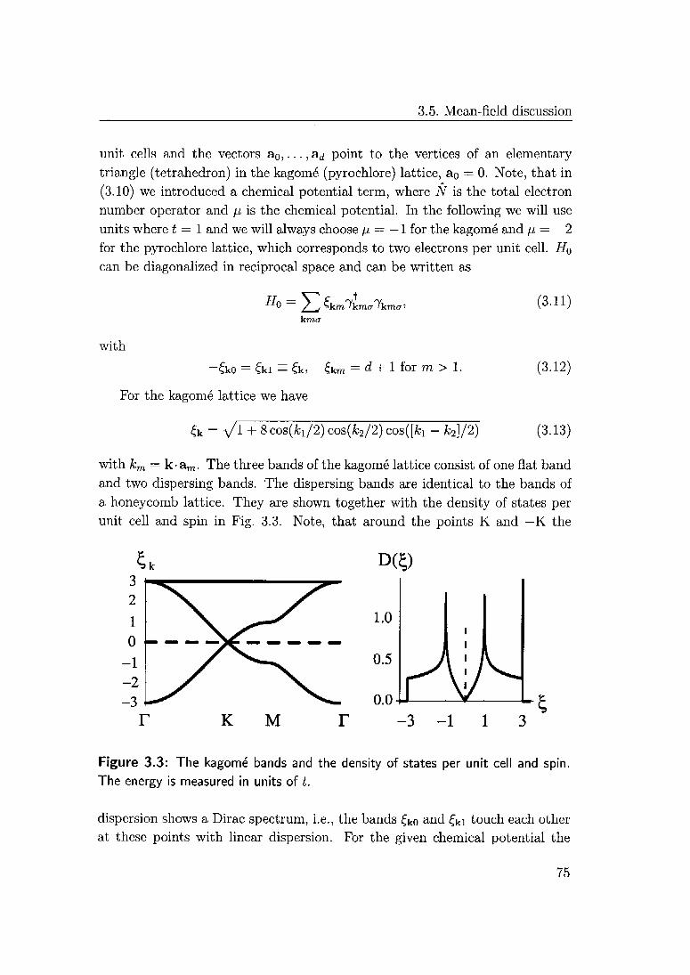
3.5. Mean-field discussion
unit cells and the vectors a0,...,ad point to the vertices of an elementary
triangle (tetrahedron) in the kagomé (pyrochlore) lattice, a0 = 0. Note, that in
(3.10) we introduced a chemical potential term, where N is the total electron
number operator and p is the chemical potential. In the following we will use
units where t — 1 and wc will always choose p — —Hot the kagomé and p — —2
for the pyrochlore lattice, which corresponds to two electrons per unit cell. Hq
can be diagonalizcd in reciprocal space and can be written as
-"0 / jSkmTkmaTkmtr'
kmir
with
-fko = £ki = £k, £km = d + 1 for m > 1.
For the kagomé lattice we have
& = V1 + 8cos(/ci/2)cos(/c2/2)cos([A;i - k2]/2)
(3.11)
(3.12)
(3.13)
with km — k • am. The three bands of the kagomé lattice consist of one flat band
and two dispersing bands. The dispersing bands are identical to the bands of
a honeycomb lattice. They are shown together with the density of states per
unit cell and spin in Fig. 3.3. Note, that around the points K and —K the
D©
1.0
0.5
0.0-JrAN
K M -3-11 3
S
Figure 3.3: The kagomé bands and the density of states per unit cell and spin.
The energy is measured in units of t.
dispersion shows a Dirac spectrum, i.e., the bands £k0 and £kl touch each other
at these points with linear dispersion. For the given chemical potential the
75

3. Bond Order Wave Instabilities in Doped Frustrated AF
Fermi surface reduces to points at K and —K and the density of states vanishes
linearly with £, i.e., we have D(£) oc |£| for small £.
For the pyrochlore lattice we have
a = /2^(cosfcm + cos^). (3.14)
y m
with k^ = Sn(^ ^ a"0 ' arc- ^he ^our bands of the pyrochlore lattice consist of
two flat bands and two dispersing bands. The dispersing bands are identical to
the bands of a diamond lattice. They are shown together with the density of
states per unit cell and spin in Fig. 3.4. Note, that £k vanishes along the lines
4
2
0
-2
-4 —
-,
rxWLT X -4-2 024
Figure 3.4: The pyrochlore bands and the density of states per unit cell and spin.
The energy is measured in units of t.
connecting X and W. The density of states also vanishes linearly at zero up to
logarithmic corrections, i.e., we have D(£) oc |£| log |£| for small £.
Systems with this form of the density of states at the Fermi level are neither
band-insulators nor normal metals, therefore, they arc sometimes called semi-
metals or zero-gap semiconductors. Although they have an even number of
electrons per unit cell and no fractionally filled bands, they have no energy gap
at the Fermi surface. Fermi surface instabilities are suppressed in this situation.
There is no Cooper instability that leads to an obvious breakdown of perturba¬
tion theory for arbitrarily small attractive interactions, as the particle-particle
polarization function involves the convergent integral J"d£.D(£)/2|£| at zero
temperature. For the half-filled honeycomb lattice it has been shown that the
Coulomb interactions lead to non-Fermi liquid behavior and that strong enough
Coulomb interactions lead to antiferromagnetic order and to the opening of a
76
>1
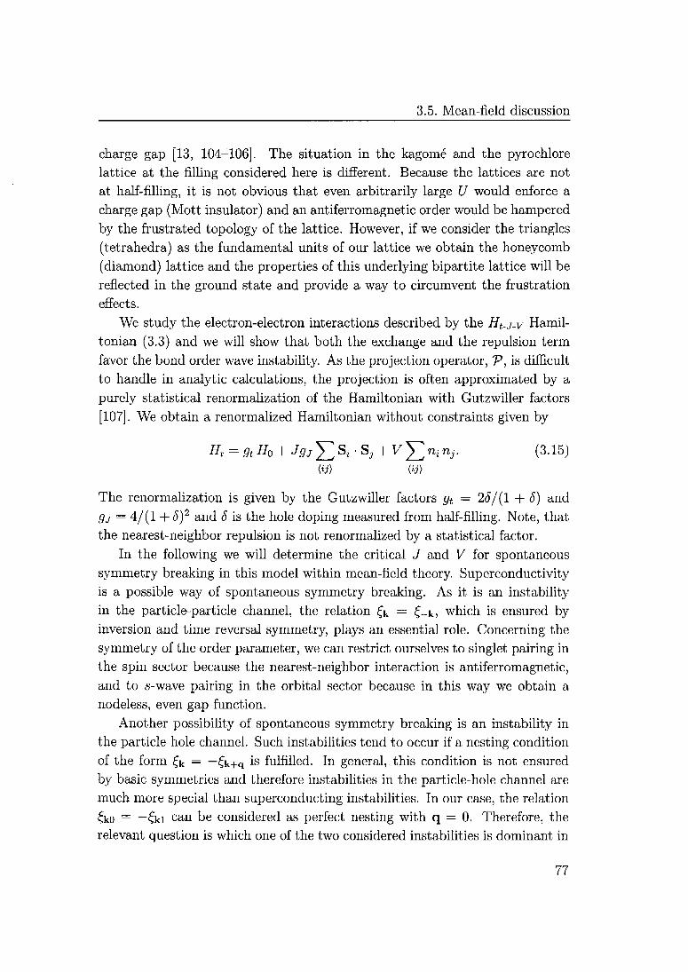
3.5. Mean-field discussion
charge gap [13, 104-106]. The situation in the kagomé and the pyrochlore
lattice at the filling considered here is different. Because the lattices are not
at half-filling, it is not obvious that even arbitrarily large U would enforce a
charge gap (Mott insulator) and an antiferromagnetic order would be hampered
by the frustrated topology of the lattice. However, if we consider the triangles
(tetrahedra) as the fundamental units of our lattice we obtain the honeycomb
(diamond) lattice and the properties of this underlying bipartite lattice will be
reflected in the ground state and provide a way to circumvent the frustration
effects.
We study the electron-electron interactions described by the Ht-j-v Hamil¬
tonian (3.3) and we will show that both the exchange and the repulsion term
favor the bond order wave instability. As the projection operator, V, is difficult
to handle in analytic calculations, the projection is often approximated by a
purely statistical renormalization of the Hamiltonian with Gutzwiller factors
[107]. We obtain a renormalized Hamiltonian without constraints given by
Hx = gtH0 + Jgj J2 Si " SJ + v J2 Ui nr (3-15)(ij) (ij)
The renormalization is given by the Gutzwiller factors gt — 28/(1 + 8) and
gj — 4/(1 + 8)2 and 8 is the hole doping measured from half-filling. Note, that
the nearest-neighbor repulsion is not renormalized by a statistical factor.
In the following we will determine the critical J and V for spontaneous
symmetry breaking in this model within mean-field theory. Superconductivityis a possible way of spontaneous symmetry breaking. As it is an instability
in the particle-particle channel, the relation £k — £_k, which is ensured byinversion and time reversal symmetry, plays an essential role. Concerning the
symmetry of the order parameter, we can restrict ourselves to singlet pairing in
the spin sector because the nearest-neighbor interaction is antiferromagnetic,
and to s-wave pairing in the orbital sector because in this way we obtain a
nodeless, even gap-function.
Another possibility of spontaneous symmetry breaking is an instability in
the particle-hole channel. Such instabilities tend to occur if a nesting condition
of the form £k ——£k+q is fulfilled. In general, this condition is not ensured
by basic symmetries and therefore instabilities in the particle-hole channel are
much more special than superconducting instabilities. In our case, the relation
fko — "~£ki can be considered as perfect nesting with q — 0. Therefore, the
relevant question is which one of the two considered instabilities is dominant in
77

3. Bond Order Wave Instabilities in Doped Frustrated AF
our system. In order to answer this question we consider the following single-
particle Hamiltonian,
atrial — Hü + AphiJph + AppiJpp (3.16)
where we have introduced the two quadratic Hamiltonians
^Ph = ££ 12 l/(i+i>*m,°cr+i>w (3-17)
^PP = Z\2Y1 l^(CH-"«»m,lCr+«'i>n,T+h-C-)- C3"18)r m^nv=±l
The idea is to calculate the expectation value of Hr (3.15) for the ground state
of iïtriai (3.16) and to choose the variational parameters App and Aph such that
this expectation value is minimized. In terms of the operators that diagonalize
Hq we can express the pairing operators as
HPh = !]ia;k7koa7kiCT + h-c-> (3-19)k<7
^PP = 1^ ekm7-kmî7kmj +h.C, (3.20)km
with the relations
& = Ckm -P, 4 = £o ~ il. (3.21)
For small values of Aph and App we can expand the ground-state expectationvalue of Hr in terms of App and Aj;h. Using the Wick theorem, we obtain up
to higher order terms
AEA2 t
(l 3J\r x V,ty^
=
ApVphlt-—(/Ph-x)-^(/Ph-x)
+ A2ppIpp It- |Vpp - x) + ~{IW + X) ] , (3-22)8
v pp /v,2
where AE is the deviation from the ground-state expectation value with Aph —
App = 0. N is the number of unit cells, t = tgt, J = 3gj, b is the number of
bonds in the unit cell, and
X = I f di(-tl-p)D(t), (3.23)0 Jç<o
'* = H«,«^ (324)
7» = ïI^Hf^- (3-25)
78
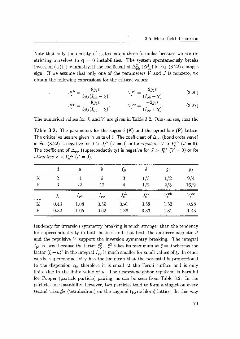
3.5. Mean-field discussion
Note that only the density of states enters these formulas because we are re¬
stricting ourselves to q — 0 instabilities. The system spontaneously breaks
inversion (U(l)) symmetry, if the coefficient of Aph (App) in Eq. (3.22) changes
sign. If we assume that only one of the parameters V and J is nonzero, we
obtain the following expressions for the critical values:
rph_
89tt ph_
2gttJc
~39j(Iph-XyVc "(Zph-X)'
{ }
/pp -S9tt
ypp -
~2gttC\ 97ïJc
~3gj(3pp-xyK
"(/pP + x)-( ]
The numerical values for Jc and Vc are given in Table 3.2. One can see, that the
Table 3.2: The parameters for the kagomé (K) and the pyrochlore (P) lattice.
The critical values are given in units of t. The coefficient of Aph (bond order wave)in Eq. (3.22) is negative for J > JPh (V - 0) or for repulsive V > Vf* (J - 0).The coefficient of App (superconductivity) is negative for J > JPp (V = 0) or for
attractive V < V (3 = 0).
d p b £o S 9t 9J
K
P
2
3
-1
-2
6
12
3
4
1/3
1/2
1/2
2/3
9/4
16/9
X -/ph -/pp Jf jw yc v?p
K
P
0.43
0.32
1.08
1.05
0.59
0.62
0.91
1.36
3.58
3.33
1.53
1.81
-0.98
-1.43
tendency for inversion symmetry breaking is much stronger than the tendency
for superconductivity in both lattices and that both the antiferromagnetic J
and the repulsive V support the inversion symmetry breaking. The integral
/ph is large because the factor £q ~ £2 takes its maximum at £ — 0 whereas the
factor (i + p)2 in the integral Ipp is much smaller for small values of £. In other
words, superconductivity has the handicap that the potential is proportional
to the dispersion ek, therefore it is small at the Fermi surface and is onlyfinite due to the finite value of p. The nearest-neighbor repulsion is harmful
for Cooper (particle-particle) pairing, as can be seen from Table 3.2. In the
particle-hole instability, however, two particles tend to form a singlet on every
second triangle (tetrahedron) on the kagomé (pyrochlore) lattice. In this way
79
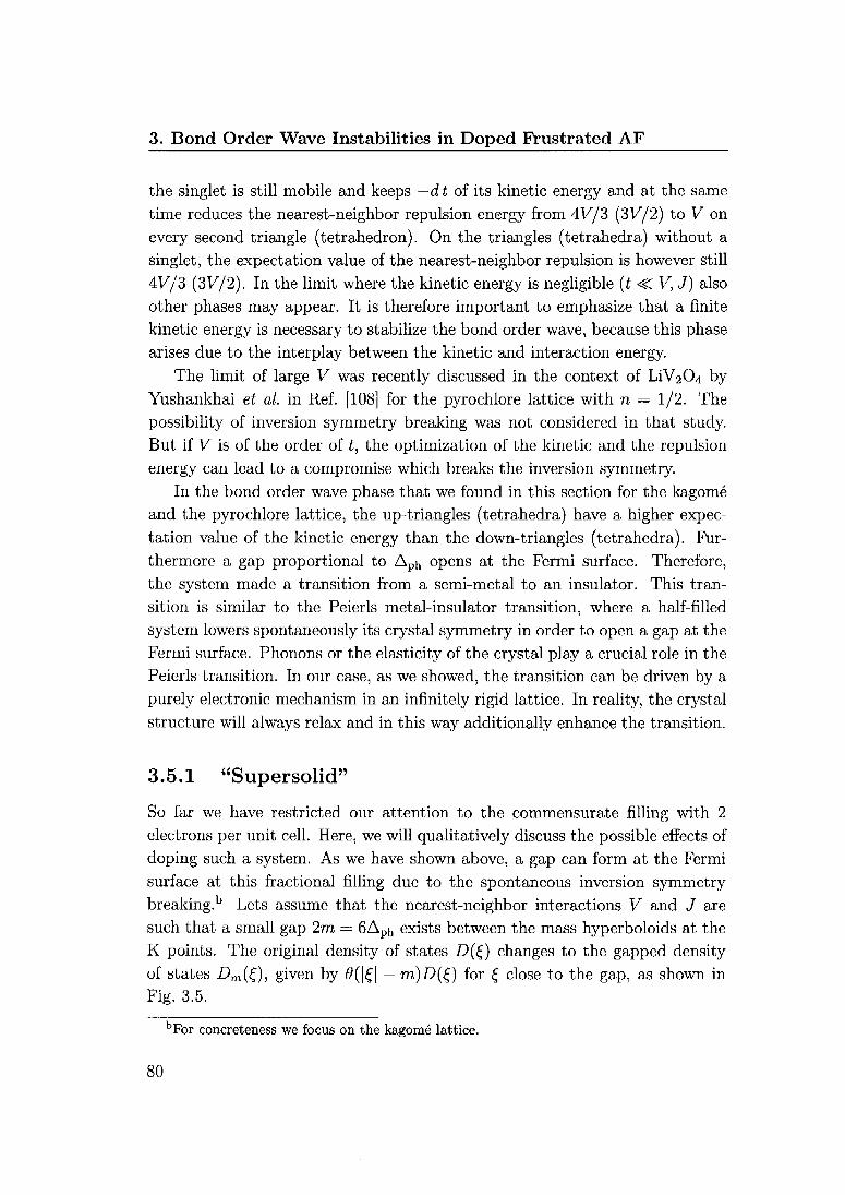
3. Bond Order Wave Instabilities in Doped Frustrated AF
the singlet is still mobile and keeps —dtoi its kinetic energy and at the same
time reduces the nearest-neighbor repulsion energy from 4V/3 (3V/2) to V on
every second triangle (tetrahedron). On the triangles (tetrahedra) without a
singlet, the expectation value of the nearest-neighbor repulsion is however still
4V/3 (3V/2). In the limit where the kinetic energy is negligible (t <£ V, J) also
other phases may appear. It is therefore important to emphasize that a finite
kinetic energy is necessary to stabilize the bond order wave, because this phase
arises due to the interplay between the kinetic and interaction energy.
The limit of large V was recently discussed in the context of LiV204 by
Yushankhai et al. in Ref. [108] for the pyrochlore lattice with n — 1/2. The
possibility of inversion symmetry breaking was not considered in that study.
But if V is of the order of t, the optimization of the kinetic and the repulsion
energy can lead to a compromise which breaks the inversion symmetry.
In the bond order wave phase that we found in this section for the kagomé
and the pyrochlore lattice, the up-triangles (tetrahedra) have a higher expec¬
tation value of the kinetic energy than the down-triangles (tetrahedra). Fur¬
thermore a gap proportional to Aph opens at the Fermi surface. Therefore,
the system made a transition from a semi-metal to an insulator. This tran¬
sition is similar to the Peierls metal-insulator transition, where a half-filled
system lowers spontaneously its crystal symmetry in order to open a gap at the
Fermi surface. Phonons or the elasticity of the crystal play a crucial role in the
Peierls transition. In our case, as we showed, the transition can be driven by a
purely electronic mechanism in an infinitely rigid lattice. In reality, the crystal
structure will always relax and in this way additionally enhance the transition.
3.5.1 "Supersolid"
So far we have restricted our attention to the commensurate filling with 2
electrons per unit cell. Here, we will qualitatively discuss the possible effects of
doping such a system. As we have shown above, a gap can form at the Fermi
surface at this fractional filling due to the spontaneous inversion symmetry
breaking.13 Lets assume that the nearest-neighbor interactions V and J are
such that a small gap 2m — 6Apt, exists between the mass hyperboloids at the
K points. The original density of states D(£) changes to the gapped density
of states Dm(£), given by 0(|£| — m)D(Ç) for £ close to the gap, as shown in
Fig. 3.5.
bFor concreteness we focus on the kagomé lattice.
80
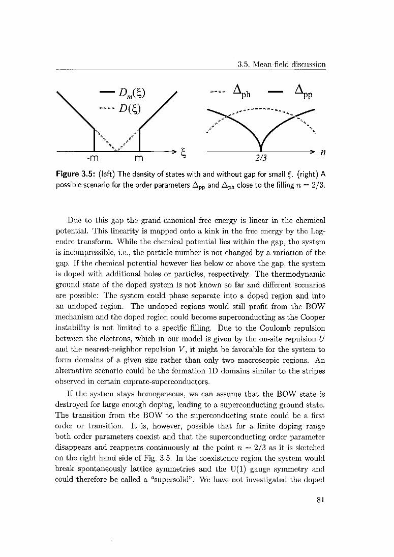
3.5. Mean-field discussion
DJS) Ph pp
> «
Figure 3.5: (left) The density of states with and without gap for small £. (right) A
possible scenario for the order parameters App and Aph close to the filling n = 2/3.
Due to this gap the grand-canonical free energy is linear in the chemical
potential. This linearity is mapped onto a kink in the free energy by the Lcg-
endrc transform. While the chemical potential lies within the gap, the system
is incompressible, i.e., the particle number is not changed by a variation of the
gap. If the chemical potential however lies below or above the gap, the system
is doped with additional holes or particles, respectively. The thermodynamic
ground state of the doped system is not known so far and different scenarios
are possible: The system could phase separate into a doped region and into
an undoped region. The undoped regions would still profit from the BOW
mechanism and the doped region could become superconducting as the Cooper
instability is not limited to a specific filling. Due to the Coulomb repulsionbetween the electrons, which in our model is given by the on-site repulsion U
and the nearest-neighbor repulsion V, it might be favorable for the system to
form domains of a given size rather than only two macroscopic regions. An
alternative scenario could be the formation ID domains similar to the stripes
observed in certain cuprate-superconductors.
If the system stays homogeneous, we can assume that the BOW state is
destroyed for large enough doping, leading to a superconducting ground state.
The transition from the BOW to the superconducting state could be a first
order or transition. It is, however, possible that for a finite doping range
both order parameters coexist and that the superconducting order parameter
disappears and reappears continuously at the point n — 2/3 as it is sketched
on the right hand side of Fig. 3.5. In the coexistence region the system would
break spontaneously lattice symmetries and the U(l) gauge symmetry and
could therefore be called a "supersolid". We have not investigated the doped
81

3. Bond Order Wave Instabilities in Doped Frustrated AF
system away from the fractional filling in detail but we believe that the study
of the ground state and the excitations of such a system is a difficult but very
interesting task.
3.6 Weak-coupling discussion
The underlying lattices of the four bisimplex lattices considered here are bi¬
partite lattices. The tight-binding bands of the bisimplex lattice follow the
tight-binding dispersion of the underlying bipartite lattice with additional flat
bands on top of them. At the particular filling of one electron per simplex the
dispersing bands of the underlying bipartite lattice are exactly half-filled. For
the two-leg ladder, the square lattice, and the honeycomb lattice, which are
the underlying lattices of the kagomé strip, the checkerboard, and the kagomé
lattice, respectively, weak-coupling RG methods at half-filling arc available
[12, 16, 106]. The t-3 model is a model for strong electronic interactions, there¬
fore, wc consider in this section the weak-coupling Hubbard model with the
interaction
Hint = uY,4Aicncrv (3'28)r
or the somewhat more general extended Hubbard interaction of Eq. (3.2). It
is possible to map this weak local Coulomb repulsion on the original bisim¬
plex lattice on an effective interaction for the underlying half-filled lattice. In
this mapping the operator Obow, whose expectation value serves as an order
parameter for the bond order wave instability, is mapped on a charge density
wave (CDW) operator Oqdw on the underlying bipartite lattice.
Although we can not expect in general that the strong coupling phases
are related to the physics at weak coupling, there are cases where the strong
coupling phase can be understood as an instability arising at weak coupling. We
will show in the following that this is the case for the one-dimensional kagomé
strip, where we find in fact a CDW instability in the underlying two-leg ladder.
The Hamiltonian (3.28) does not directly drive the BOW instability on the
bisimplex lattice. It turns out that also the derived effective interaction on
the underlying lattice does not drive the CDW instability directly, i.e., the
CDW instability can not be obtained as a mean-field instability of the effective
interaction but occurs due to higher order and not due to first order terms of
the interaction.
82
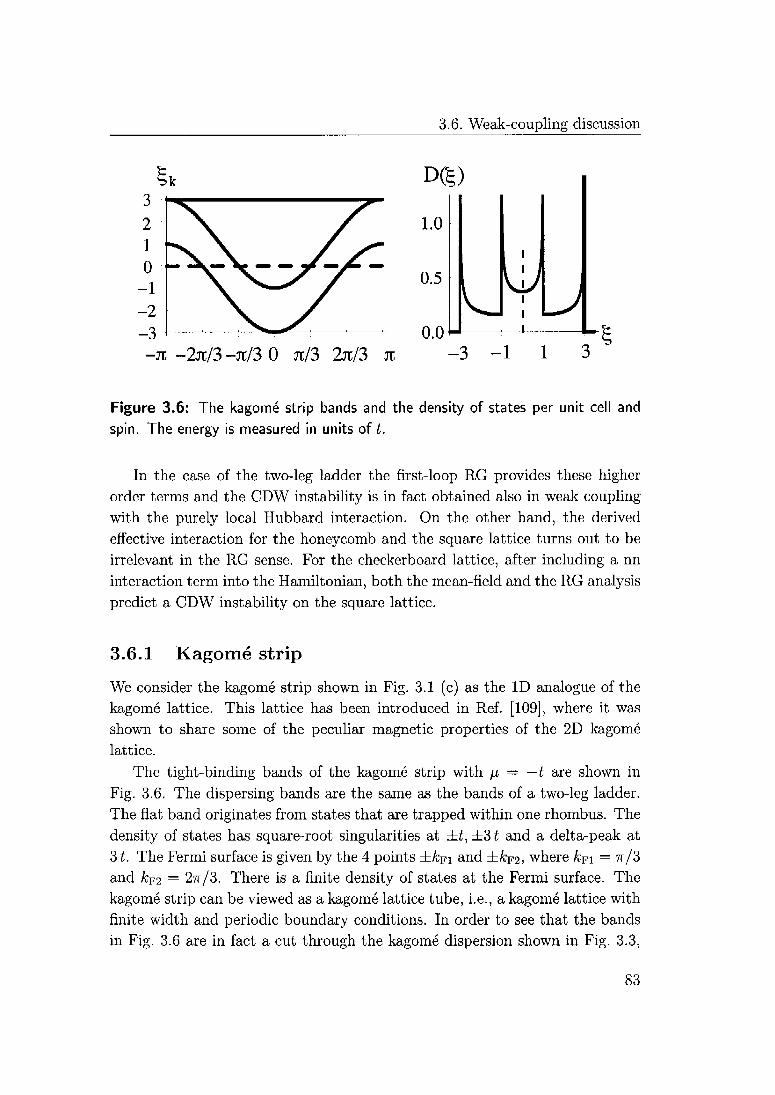
3.6. Weak-coupling discussion
-jt -2jt/3 -Jt/3 0 jt/3 2jt/3 Jt
1.0
0.5
0.0^
VjW
-3 -1 1
Figure 3.6: The kagomé strip bands and the density of states per unit cell and
spin. The energy is measured in units of t.
In the case of the two-leg ladder the first-loop RG provides these higher
order terms and the CDW instability is in fact obtained also in weak coupling
with the purely local Hubbard interaction. On the other hand, the derived
effective interaction for the honeycomb and the square lattice turns out to be
irrelevant in the RG sense. For the checkerboard lattice, after including a nn
interaction term into the Hamiltonian, both the mean-field and the RG analysis
predict a CDW instability on the square lattice.
3.6.1 Kagomé strip
We consider the kagomé strip shown in Fig. 3.1 (c) as the ID analogue of the
kagomé lattice. This lattice has been introduced in Ref. [109], where it was
shown to share some of the peculiar magnetic properties of the 2D kagomé
lattice.
The tight-binding bands of the kagomé strip with p = —t are shown in
Fig. 3.6. The dispersing bands are the same as the bands of a two-leg ladder.
The flat band originates from states that are trapped within one rhombus. The
density of states has square-root singularities at ±t,±3t and a delta-peak at
31. The Fermi surface is given by the 4 points ±&fi and ±kF2, where kF\ — n/3and kF2 — 27r/3. There is a finite density of states at the Fermi surface. The
kagomé strip can be viewed as a kagomé lattice tube, i.e., a kagomé lattice with
finite width and periodic boundary conditions. In order to see that the bands
in Fig. 3.6 are in fact a cut through the kagomé dispersion shown in Fig. 3.3,
83
3. Bond Order Wave Instabilities in Doped Frustrated AF
one has to shift one of the dispersing bands by n. This difference arises because
our notation is chosen to emphasize the similarities of the kagomé strip to the
two-leg ladder.
In contrast to the kagomé and the pyrochlore lattice, the density of states
at the Fermi surface is finite for the kagomé strip and we therefore expect
qualitative changes in this ID system even for weak interactions. We perform
a weak-coupling RG and bosonization analysis for the kagomé strip, and we
show that the bond order wave instability is already present for arbitrary weak
coupling. In this section we will only present the results of this analysis and
refer to App. B.l.l for further details.
We derive an effective interaction for the two-leg ladder, that corresponds
in weak coupling to the local Coulomb repulsion on the kagomé strip (3.28).In this derivation we can drop terms that involve the high energy states of
the flat band and focus on the states in the dispersing bands. We denote the
annihilation operator of these states by 7^ — 7^ where k is the momentum
along the strip and i — 1, 2 is the band index. If we rewrite the Hamiltonian
üfint of Eq. (3.28) in terms of these new operators we obtain the interaction.
T T
#int -j Yl Ski...«* 7klT7i2i7k3i7k4Î, (3-29)
k!...k4
where the prime over the sum restricts the sum to momentum conserving k-
values. For weak interaction we can replace k; in ,9k,...k4 by (kFil,ii) and we
obtain the simple expression
#ki...k4 = e~'2 (8hi28i3i4 + 8ili38i2i4 + 8hi48i2l3)/6: (3.30)
where q — ki + k2 — k3 — A;4.
The effective interaction (3.29) can now be expressed in terms of left and
right moving currents and in this way we find the initial values for the RG
equations of the two-leg ladder. The integration of the RG equations with
these initial values converges to an analytic solution that was identified by
bosonization techniques as a charge density wave solution (CDW) solution [16].This means that the operator
OCDW =
J Yl 7fciff7fc+^,2a + ^k+n,2a%la (331)ka
acquires a finite value. The bond order wave order-parameter on the kagomé
strip is given by the expectation value of an operator Obow-
84
3.6. Weak-coupling discussion
The operators Oqdw and Obow transform identically under all symmetries
of the system and, therefore, they describe the same phase.
In addition, Ocdw is the effective operator on the two-leg ladder for Obow>
i.e., if one does the same substitutions as we did for deriving Eq. (3.29) one
sees that Obow ~~* Ocdw> if °ne chooses the right prefactor in the definition of
Obow-
We have shown that the bond order wave instability that is expected to
occur at rather strong interactions according to the arguments of the preceding
sections, is in fact already present in weak coupling for the one-dimensional
kagomé strip. The density matrix renormalization group (DMRG) results in
Sec. 3.7 provide convincing evidence that the same symmetry breaking also
occurs in the t-3 model.
3.6.2 Checkerboard lattice
The tight-binding bands of the checkerboard lattice consist of an upper flat
band and a lower dispersive band. The lower band is identical to the tight-
binding band of the square lattice and touches the flat band at the M points.
For the filling n — 1/2 the dispersive band is half-filled, and the Fermi surface is
quadratic and perfectly nested with the nesting vector (n, n). The corners (n, 0)and (0,7r) of the Fermi surface are saddle points and lead to a logarithmically
diverging density of states.
For the checkerboard lattice we study the extended Hubbard Hamiltonian
with the interaction of Eq. (3.2) including nn antiferromagnetic J exchange and
nn repulsion V. We choose the chemical potential p = —2t which correspondsto a half-filled lower band and we can write
#o = X^k7L7k(T + 4tiVflat with Çk = -2*(cosfc1-f-cosA;2). (3.32)k<7
Aflat counts the number of electrons in the flat band at 4t. In the weak-
coupling limit these states do not affect the low-energy physics of the system
and therefore they will be dropped in the following analysis.
For small couplings U, V and J we obtain an effective interaction Hamilto¬
nian (App. B.1.2) given by
-"int — l^j 2.^1 ^ki...k4 ^7k1Cr7k2CT'7k3(T'7k4CT> (3.33)ki.,.k4 era'
85

3. Bond Order Wave Instabilities in Doped Frustrated AF
with
2
£k,..k4 - Y(U< + 2H,3- J<Jel<AA*
2
+ E(4^Wk2k3 - 2J/^k3/k2k4) (3.34)i/=i
with e£ - cos(k„/2), /£k, - e£_k,e£e£,, V - V- J/4, q - ki + k2-k3-k4, and
%' — q — 2(kj — kj). The two saddle points Pi — (0,7r) and P2 — (n, 0) of the
dispersion lead to the logarithmic divergence of the density of states. Therefore,
we can characterize very weak interactions by the values of the function #ki...k4
where all four momenta ki • • • ki lie on one of the two saddle points. Following
the notation of Ref. [12] we have the following four couplings constants:
ki,k3 eFi
<7k,...k4 = <_
n, ,
_ o(3-35)
ki,k2GPi
J ki... k4 G Pi
From the RG equations of Ref. [12] we see that for positive values of U, V, and
J the coupling g\ flows to —oo and the coupling g2 flows to +oo,c whereas the
other couplings flow to 0. This shows that the charge density wave susceptibility
is diverging most rapidly under the RG flow. As shown in Fig. 3.7 the CDW
instability on the square lattice corresponds to the BOW instability on the
checkerboard lattice, i.e., both instabilities break exactly the same symmetries.
Note, that within the framework of this RG scheme, we can not determine
whether a usual CDW or a so-called charge flux phase, which is a CWD with
a (i-wave form factor, is stabilized. In the following we will denote these two
phases with s-CDW and <i-CDW. (Note, that for J — 0 only the coupling g2
diverges. In this case we can not even determine whether a CDW of SDW
phase is stabilized.) In order to show, that the s-CDW phase is in fact favored
over the ti-CDW, at least in a mean-field analysis, we restrict the interaction
Hamiltonian (3.33) to the CDW channel and obtain:
#CDW =
JTj Y VW Y 7L7k+Q,<r7k'+Qy7k'<r' (3.36)kk' aa'
cFor V < 0 <?2 flows to 0, but also in this case the CDW phase is stabilized.
86
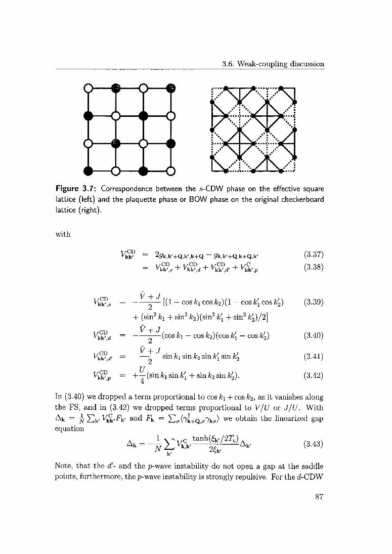
3.6. Weak-coupling discussion
IX ** ' +^ JT X *
I X **. J x**+ m
Figure 3.7: Correspondence between the s-CDW phase on the effective square
lattice (left) and the plaquette phase or BOW phase on the original checkerboard
lattice (right).
with
yCD
^kk' Sgk.k'+C^k'.k+Q — flfk,k'+Q,k+Q,k'
^CD rCD CD—
vYk',s + ^kk'.d + ^kk'^' + ^kk
(3.37)
(3.38)
t/CD^kk'.s
1/CD
yCD
yCD
V + 3[(1 — cosfciCosA;2)(l — cos k[ cos k2) (3.39)
+ (sin2 fci + sin2 /c2)(sin2 fci + sin2 k'2)/2]V + J
(cos ki — cos /c2)(cos ^i — cos k2)
sin fci sin k2 sin A;^ sin k2
2
V + J
U— +—(sin k\ sin k[ + sin k2 sin &2).
(3.40)
(3.41)
(3.42)
In (3.40) we dropped a term proportional to cos k\ + cos k2, as it vanishes alongthe FS, and in (3.42) we dropped terms proportional to V/U or J/U. With
Ak = jfT2k'VkL'Fw and Pk = 2-},t(7k+Q)(T7k<T) we obtain tiie linearized gap
equation
A _1STvc tanh(^'/2Tc)
2&At/ (3.43)
Note, that the d'- and the p-wave instability do not open a gap at the saddle
points, furthermore, the p-wave instability is strongly repulsive. For the rf-CDW
87

3. Bond Order Wave Instabilities in Doped Frustrated AF
state the pair potential (3.40) is separable and the linearized gap equation can
be written in the simpler form
1y + J^. , ,
.2tanh(£k/2rcd)
1 ^ ___2J(cosfcl_ cos*;2)2 ^
cJ. (3.44)
The pair potential for the s-CDW state (3.39) is not separable. But if we neglect
for a moment the second line in (3.39) we obtain an analogous expression to
(3.44) for the critical temperature of the s-CDW with cos k\ — cos k2 replaced
by 1 — cos ki cos k2. As on the FS we have cos k2 — — cos ki and as |2 cos ki\ <
1 + cos2fci, we know that the critical temperature of the s-CDW phase is
higher than the critical temperature of the d-CDW phase. Including the non-
negative second term in (3.39) would only lead to a further increase of the
critical temperature. Note, that the magnitude of the d- and the s-CDW
potentials are identical for the momenta on the saddle points. Therefore it is
not surprising that they cannot be distinguished by the two-patch RG method.
However, in the mean-field we can see that the s-CDW is favored over the
d-CDW state, as it opens a finite gap along the entire FS. It is possible to do
such a mean-field analysis also for SDW and superconducting instabilities. For
superconductivity we have the Cooper channel
Hsc = Àj}2v£tL-r-w-r-WY** (3-45)kk' oa'
that can be projected onto the different symmetry channels as follows:
V&9 = <?k,-k,-k',k' = <?,, + V$,d + V&9 d, + V&9p
(3.46)
V&s - \ (3-47)
V$td = it(cos fa - cos fo)(cos k[ - cos k2) (3.48)
^kk^d' =
—ö—s*n ^1 s*n ^2 s*n ^i s*n ^2 (3.49)
^kkv —
—z—(2 + cos ki cos k\ + cos k2 cos k'2)
(sin k\ sin k[ + sin k2 sin k'2) (3.50)
where we again set cos &i + cos k2 — 0 and neglected terms proportional to J/Uand V/U in the potentials containing U (3.47,3.48). We find strong repulsion
88

3.6. Weak-coupling discussion
(oc U) in the d- and in the s-wave channel, and only weaker (oc V, J) and
mainly repulsive interactions in the d'- an the p-wave channel.0 Furthermore,
the df- an the p-wave channels do not open a gap at the saddle points. It is
therefore quite clear, that the superconducting instabilities can not compete
with the s-CDW instability.
For the pair SDW instabilities, we obtain the Hamiltonian
#SDW =
T^Y VM Yl ^k^k+Q^k'+Q.^kV', (3.51)kk' aa'
where the SDW pair potential is given by
^kk' = -9k,k'+Q,k+Q,k' = Vkk,s + Vkk,d + Vkk,d, + Vkk,p (3.52)
and with the same approximation as before we have
Vkk,s = —— [(1 — cos hi cos k2)(l — cos k\ cos k'2) (3.53)
+(2 - cos2fci - cos2A;2)(2 - cos2/si - cos2fc2)/8]£.
2Vku!,d = -—(cos ki - cos k2)(cos k[ - cos k'2) (3.54)
V
Vkk,d, = —— sin k\ sin k2 sin k[ sin k'2 (3.55)
Vkw,p — ~~r(s^n ^i sm ^i + sm ^2 sm ^2)- (3.56)
These SDW potentials are identical to the CDW potentials in Eqs. (3.39-3.42)if we replace only V + J by V and U by —U. For J > 0 we have V + J > V and
therefore the s-, d- and d'-CDW instabilities are favored over the corresponding
SDW instabilities.
The p-SDW instability is strongly attractive but has the handicap, that it
does not open a gap at the saddle points, therefore for weak interactions the
s-CDW state will still be favored over the p-SDW state, i.e., for interaction
parameters (U, V, J) given by (au, av, aj) we can find for all positive values of
(u,v,j) an a0 such that for 0 < a < a0 the s-CDW state is stabilized.
In conclusion, in this section we showed with two-patch RG and mean-field
arguments, that for weak enough repulsive and antiferromagnetic interactions
the s-CDW phase is stabilized in the effective model on the square lattice.
This CDW phase corresponds to the BOW phase on the original checkerboard
lattice.
jIn the p-wave channel we would have triplet superconductivity
89

3. Bond Order Wave Instabilities in Doped Frustrated AF
3.6.3 Kagomé lattice
The underlying lattice of the kagomé lattice is the bipartite honeycomb lat¬
tice. The filling considered here corresponds to a half-filled honeycomb lattice,
where the Fermi surface consists of only two points. It is possible to derive
an effective interaction for the honeycomb lattice that corresponds to the weak
onsite Coulomb repulsion (3.28) on the kagomé lattice. The effective Hamil¬
tonian on the honeycomb lattice contains onsitc terms and nn interaction and
pair hopping terms and is given by
Hint - f£ "*"*! + £ (Vnini ~ JSi • S^ " Atyijjifji + h.c]) , (3.57)1 (ij)
where V = U/18, J = 2J - 2U/9. The sum J2i (2~2(ij)) runs over a11 sites
(bonds) of the honeycomb lattice. As the Hamiltonian Hmt contains, e.g., nn
repulsion terms, one could expect that the mean-field analysis of this effective
interaction Hamiltonian could predict a CDW instability on the honeycomb
lattice, that would correspond to the BOW instability on the kagomé lattice.
Calculating all the Hartree-Fock energies using a CDW trial wave function, we
find that the interaction energy does not depend on the CDW order parameter
but the kinetic energy increases as the CDW order is build up. The situation
does therefore not change by going to the effective Hamiltonian: In the same
way as the onsite Hubbard energy does not depend on the BOW strength,
the effective interaction energy on the square lattice does not depend on the
CDW order parameter in the mean-field analysis. In order to see the CDW
instability on the checkerboard lattice in mean-field we should also include
nn interaction terms in the original Hamiltonian on the kagomé lattice. The
mean-field analysis of such a Hamiltonian has already be done in Sec. 3.5.
The onsite Hubbard interaction (3.28) produces onsite and nn interaction
terms in the effective interaction. As the density of states vanishes linearly at
the Fermi level as seen in Fig. 3.3 such an effective short-ranged interaction is
irrelevant in the RG sense [106].In conclusion, we found for the kagomé strip that already the onsite Hub¬
bard interaction is sufficient to produce the CDW instability in the weak-
coupling RG analysis. For the checkerboard lattice, we had in addition to
include nn neighbor interactions to observe the CDW instability on the square
lattice both in mean-field and in the two-patch RG. For the kagomé lattice
we calculated the effective Hamiltonian for the Hubbard model on the hon¬
eycomb lattice, but no CDW instability could be obtained in mean-field. In
90

3.7. Numerical results
fact, according to RG calculations on the half-filled honeycomb lattice, there
is no instability in weak-coupling on the honeycomb lattice for any kind of
short-ranged interactions [106].
3.7 Numerical results
In this section we compare the analytical predictions obtained in the preced¬
ing sections to various numerical results on one- and two-dimensional systems.
We will first discuss some exact diagonalization results for both the kagomé
lattice at n — 2/3 and the checkerboard lattice at n — 1/2. Then we move to
the kagomé strip at n — 2/3, where we report extensive density matrix renor¬
malization group calculations [11], both for the t-J and the Hubbard model.
In essence the numerical results corroborate the analytical predictions on the
presence of a bond order wave instability at a particular doping.
3.7.1 Kagomé lattice
The analytical arguments presented in Sec. 3.3, 3.4, and 3.5 predict a bond
order wave instability at filling n — 2/3. In finite, periodic systems this insta¬
bility can be detected with a correlation function of the bond strength, either of
the kinetic term or the exchange term. Here we chose to work with the kinetic
term, but the exchange term gives similar results. The correlation function is
defined as:
CKin[(i,j),(Kl)} = (Kin(i,j) Kin(M)) " (Km(i,j))(Km(k,l)),
where
Kin(z, j) = - 134^ + h.c, (3.58)(7
and (i, j) and (k, I) denote two different nearest-neighbor bonds of the kagomé
lattice, that have no common site. This correlation function has been calcu¬
lated for all distances in the ground state of a finite kagomé sample with 21
sites, containing 7 holes at J/t — 0.4. The result is plotted in Fig. 3.8. The
reference bond uniquely belongs to a certain class of triangles (up-trianglcs in
our case). Based on the theoretical picture one expects the correlation function
to be positive for all bonds on the same type of triangles and negative on the
others. This is indeed what is seen in Fig. 3.8. We have also calculated the
same quantity for J/t — 1 and J/t — 2 and the bond order wave correlations
91
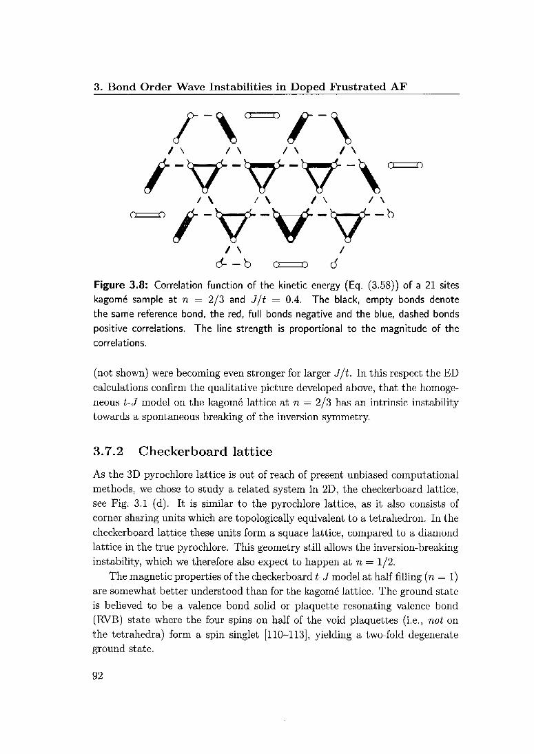
3. Bond Order Wave Instabilities in Doped Frustrated AF
/VVYv/\ / \ / \ /\
/tfV"1/ \ /
(3— b o=o Ô
Figure 3.8: Correlation function of the kinetic energy (Eq. (3.58)) of a 21 sites
kagomé sample at n — 2/3 and J/t = 0.4. The black, empty bonds denote
the same reference bond, the red, full bonds negative and the blue, dashed bonds
positive correlations. The line strength is proportional to the magnitude of the
correlations.
(not shown) were becoming even stronger for larger J/t. In this respect the ED
calculations confirm the qualitative picture developed above, that the homoge¬
neous t-J model on the kagomé lattice at n = 2/3 has an intrinsic instability
towards a spontaneous breaking of the inversion symmetry.
3.7.2 Checkerboard lattice
As the 3D pyrochlore lattice is out of reach of present unbiased computational
methods, we chose to study a related system in 2D, the checkerboard lattice,
see Fig. 3.1 (d). It is similar to the pyrochlore lattice, as it also consists of
corner sharing units which are topologically equivalent to a tetrahedron. In the
checkerboard lattice these units form a square lattice, compared to a diamond
lattice in the true pyrochlore. This geometry still allows the inversion-breaking
instability, which we therefore also expect to happen at n — 1/2.The magnetic properties of the checkerboard t-J model at half-filling (n — 1)
are somewhat better understood than for the kagomé lattice. The ground state
is believed to be a valence bond solid or plaquette resonating valence bond
(RVB) state where the four spins on half of the void plaquettes (i.e., not on
the tetrahedra) form a spin singlet [110-113], yielding a two-fold degenerate
ground state.
92
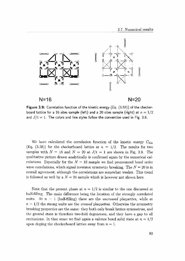
3.7. Numerical results
0=0=0 j> —a 0=
=0 c£ —^o 0=0
N=16 N=20
Figure 3.9: Correlation function of the kinetic energy (Eq. (3.58)) of the checker¬
board lattice for a 16 sites sample (left) and a 20 sites sample (right) at n — 1/2and J/t ~ 1. The colors and line styles follow the convention used in Fig. 3.8.
We have calculated the correlation function of the kinetic energy Cxin
(Eq. (3.58)) for the checkerboard lattice at n — 1/2. The results for two
samples with N — 16 and N — 20 at J/t — 1 arc shown in Fig. 3.9. The
qualitative picture drawn analytically is confirmed again by the numerical cal¬
culations. Especially for the N = 16 sample we find pronounced bond order
wave correlations, which signal inversion symmetry breaking. The N — 20 is in
overall agreement, although the correlations are somewhat weaker. This trend
is followed as well by a N — 24 sample which is however not shown here.
Note that the present phase at n — 1/2 is similar to the one discussed at
half-filling. The main difference being the location of the strongly correlated
units. At n = 1 (half-filling) these are the uncrossed plaquettes, while at
n — 1/2 the strong units are the crossed plaquettes. Otherwise the symmetry
breaking properties are the same: they both only break lattice symmetries, and
the ground state is therefore two-fold degenerate, and they have a gap to all
excitations. In that sense we find again a valence bond solid state at n — 1/2
upon doping the checkerboard lattice away from n — 1.
93

3. Bond Order Wave Instabilities in Doped Frustrated AF
(a) -lZa(4aCja)
(b) (S.-S,
/VvVvVvVvVvVvVvVvVvVvYvV
Figure 3.10: DMRG results for a L = 24 kagomé ladder at J/t = 0.4 and
n = 2/3. (a) Local bond strength deviation of the kinetic term. Red, full bonds
are stronger (lower in energy) than the average kinetic energy per bond. Blue,
dashed bonds are weaker than average bonds, (b) Local bond strength deviation
of the exchange term. The color pattern are the same as in the upper panel. The
thickness of the bond denotes the deviation from the average value per bond. Note
that the pattern of the kinetic and the exchange term are in phase.
3.7.3 Kagomé strip
The kagomé strip, being a ID system, offers the opportunity of DMRG simu¬
lations; thus allowing a rather detailed numerical study of large systems. We
first discuss the properties of the t-J model at n — 2/3 on this lattice, and
then make a connection to the analytical weak-coupling results obtained in
Sec. 3.6.1 by investigating the Hubbard model at different values of U. In both
cases we report sound numerical evidence for the presence of the bond order
wave instability for a large range of interactions strengths.
In contrast to the periodic systems considered above within ED, the DMRG
works most efficiently for open boundary conditions. In the present context this
has the additional advantage that for even length L of the strip only one of the
two degenerate ground states is favored, and we can directly measure the local
bond strength. For the purpose of illustration we show the local bond strengths
for a system of L = 24 in Fig. 3.10. The upper panel shows the difference of the
local kinetic energy with respect to the average, while the lower panel shows the
local expectation value of the spin exchange term, using the same convention.
The calculated pattern resembles the schematic picture drawn in Fig 3.1 (c).In order to address the behavior in the thermodynamic limit we measure the
94
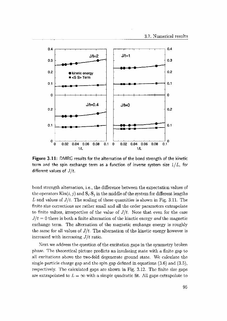
3.7. Numerical results
0.4
0.3
0.2
0.1
0
0.2
0.1
00 0.02 0.04 0.06 0.08 0.1 0 0.02 0.04 0.06 0.08 0.1
1/L 1/L
Figure 3.11: DMRG results for the alternation of the bond strength of the kinetic
term and the spin exchange term as a function of inverse system size 1/L, for
different values of J/t.
bond strength alternation, i.e., the difference between the expectation values of
the operators Kin(z, j) and Sj-S^ in the middle of the system for different lengths
L and values of J/t. The scaling of these quantities is shown in Fig. 3.11. The
finite size corrections are rather small and all the order parameters extrapolate
to finite values, irrespective of the value of J/t. Note that even for the case
J/t — 0 there is both a finite alternation of the kinetic energy and the magnetic
exchange term. The alternation of the magnetic exchange energy is roughly
the same for all values of J/t. The alternation of the kinetic energy however is
increased with increasing J/t ratio.
Next we address the question of the excitation gaps in the symmetry broken
phase. The theoretical picture predicts an insulating state with a finite gap to
all excitations above the two-fold degenerate ground state. We calculate the
single-particle charge gap and the spin gap defined in equations (3.6) and (3.5),
respectively. The calculated gaps are shown in Fig. 3.12. The finite size gaps
are extrapolated to L — oo with a simple quadratic fit. All gaps extrapolate to
U.H
0.3
0.2
0.1
0.2
0.1
J/t=2
kinetic energyi <S S> Term
- -»-
H—i—I—i—h
J/t=0.4
• • •-
_l * L_.
J/t=1
H 1 I 1 1 h
J/t=0
•• • »
95
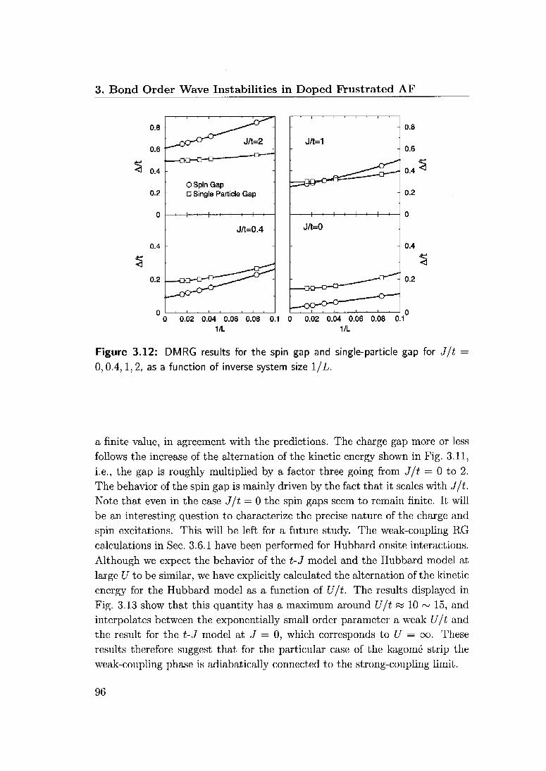
3. Bond Order Wave Instabilities in Doped Frustrated AF
0.8
0.6
0.4*3
0.2
0
0.4
%
0.2
00 0.02 0.04 0.06 0.08 0.1 0 0.02 0.04 0.06 0.08 0.1
1/L 1/L
Figure 3.12: DMRG results for the spin gap and single-particle gap for J/t =
0,0.4,1,2, as a function of inverse system size 1/L.
a finite value, in agreement with the predictions. The charge gap more or less
follows the increase of the alternation of the kinetic energy shown in Fig. 3.11,
i.e., the gap is roughly multiplied by a factor three going from J/t = 0 to 2.
The behavior of the spin gap is mainly driven by the fact that it scales with J/t.Note that even in the case J/t — 0 the spin gaps seem to remain finite. It will
be an interesting question to characterize the precise nature of the charge and
spin excitations. This will be left for a future study. The weak-coupling RG
calculations in Sec. 3.6.1 have been performed for Hubbard onsite interactions.
Although we expect the behavior of the t-J model and the Hubbard model at
large U to be similar, we have explicitly calculated the alternation of the kinetic
energy for the Hubbard model as a function of U/t. The results displayed in
Fig. 3.13 show that this quantity has a maximum around U/t œ 10 ^ 15, and
interpolates between the exponentially small order parameter a weak U/t and
the result for the t-J model at J — 0, which corresponds to U — oo. These
results therefore suggest that for the particular case of the kagomé strip the
weak-coupling phase is adiabatically connected to the strong-coupling limit.
0.8
0.6
< 0.4
0.2
0
0.4
%
0.2
O Spin Gapd Single Particle Gap
___t_t_H.__+__l—,—|—,_
J/t=0.4
96

3.8. The Dirac points of the kagomé lattice
infinity
Figure 3.13: DMRG results for the kinetic energy alternation for Hubbard kagomé
strips at n — 2/3 of length L — 32 and L = 48. The modulation is non-
monotonous as a function of U/t and shows a maximum around U/t & 10 ~ 15.
3.8 The Dirac points of the kagomé lattice
So far we only considered particle-hole instabilities on the bisimplex lattices,that break lattice symmetries, i.e., the inversion symmetry or translational
symmetry. In this last section we discuss the unusual properties of electrons on
the kagomé lattice with broken inversion and broken time-reversal symmetry.
The ideas of this section are based on previous work by Haldane [5], who
presented a similar discussion for the honeycomb lattice. We will show, that the
effects described by Haldane for the honeycomb lattice can also be obtained on
the kagomé lattice, in fact, it turns out that it is even more natural to describe
these effects on the kagomé lattice.
As can be seen from Fig. 3.3 the tight-binding dispersion of the kagomé
lattice has two so-called Dirac points at the points K and K'. At such a point,
two bands touch with linear dispersion and produce a double cone. At this par¬
ticular filling the low-energy physics can therefore be described by two species
of chiral "(2+l)-dimensional" relativistic fermions. The presence of an equalnumber of Weyl fermions with opposite chirality is not accidental. Apply-
97

3. Bond Order Wave Instabilities in Doped Frustrated AF
ing a homotopy theory argument Nielsen and Ninomiya could prove that this
kind of "fermion doubling" occurs for all quadratic fermion models on a lattice
[114, 115]. These Dirac points and the related anomalous phenomena have been
intensely discussed for the honeycomb lattice. Semenoff studied the effects of
broken inversion symmetry on the honeycomb lattice [4], leading to a massive
dispersion of the fermions, and Haldane discussed the quantum Hall phases in
the system with broken time reversal and inversion symmetry [5].In this section we will show how and to which extent the physics of the
honeycomb lattice can be mapped onto the physics of the kagomc lattice. We
omit the spin indices, a, which would be only a bystander in the following
discussion. The notation used on the kagomé lattice is shown in Fig. 3.14. The
lattice vectors ax — (a, 0), a2 — a(—1, VZ)/2, and a3 = a(—l,—\/3)/2 satisfy
a: + a2 + a3 = 0. We allow for different hopping parameters tv and tA on the A
and V triangles. With this notation, we obtain the tight-binding Hamiltonian
Figure 3.14: The notation on the kagomé lattice.
H = — 2_^ y^Cr,m+lCr,m-l + ^ACr,m+lcr+am,m-l + h.C I (3.59)TWl
We define the Fourier transformed operators as
Crm-~Y] eik.[r+(am.1-am+1)/6]Ckmj (360)VAT
k
98

3.8. The Dirac points of the kagomé lattice
where N is the number of unit cells. The Hamiltonian (3.59) can be written as
H = -Y[(t^~ikam/2 + t>^n/2)Clrn+^rn^ +h.C.] (3-61)km
= "2Z { K* + iA") ^s(km/2) - iA' sin(A;m/2)] c{tm+lckjm_x + h.c.} ,
km
and in the last line we have set
tv^t + A, tA = t-A, A - A' + iA", t, A', A" e R, (3.62)
and wrote km instead of k-am. The terms proportional to A' break the inversion
symmetry, whereas the terms proportional to A" break time reversal symmetry.
In the following we focus on 1/3-filling and introduce a chemical potential
p = —t. For A = 0, the electron filling is 1/3 and the Fermi surface (FS) is
reduced to the two K points
K=-K'=-S(i)- (3'63)
The density of states at the "Fermi points" vanishes and the dispersion is linear
and cone shaped around the K points;
a/3Erf(k + K) = E±(k + K') = ±-|k|a£ + C((|k|a)2). (3.64)
We are interested, how the dispersion changes after introducing a finite
A. At the T point the energies do not change for a finite value of A'. The
degenerate states at the F point only split if time reversal symmetry is broken
by a finite value of A". At the M points the energies do not change in first
order perturbation theory, as the eigenstates arc real and not degenerate and
the perturbation is imaginary. At the points K and K' the Hamiltonian for
A — 0 including chemical potential is given by
(3.65)
This matrix is diagonalized by the unitary transformation
^tH0^ = diag[0,0,3t] with U - -^ f u u2 1 ] (3.66)
99

3. Bond Order Wave Instabilities in Doped Frustrated AF
and with u = el27r/3. For finite A we have the perturbation matrices H%
(a — ±1) at the points aK given by
H% = AQ#i with H1= \ i 0 i (3.67)
and with AQ = (A" - a^/3A').This leads to a splitting of the degenerate states by iv^A" at the points
aK. Note, that the splitting is symmetric if A is real or imaginary (fermion
doubling). However, in general the splitting is asymmetric and for A" — ±y/ZA'it is absent at one of the K points.
If we move a little bit away form the points K and K' to the points 8ka —
k — aK, assuming however that |<5ka|a <C 1 and keeping only terms of first-
order in \8ka\ in the Hamiltonian, we obtain an additional perturbation
^/ 0 ök$ 8k% \
H£ = a~- Ski 0 -6kf . (3.68)
V 6k% -6k? 0 /
Calculating up to first order in A' and |<5kö|, we can restrict the Hilbert space
to the space spanned by the first two columns of U and we obtain
[U (H0 + HA + Hk)U]2x2 - I_Xa{SK _ .6k^ ^Aa
where we have set A = \[Zta/2 and used thatc
8k« + u>Sk% + u28k% = 3a(<5*£ + \5k^)/2.
We obtain an effective Hamiltonian
H = Y^ Y^ ( V'Pa\ ( -m^2 -<^c(Px + iPy)
where pa ~ HS\i.a,
(3.69)
(3.70)
\/h = ^^, m^c2 = V3AQ - V3(A" - aVZA') (3.71)2h
"ok" — Sk\a ex and ök = SU. • ey, where &XiV arc the unit vectors.
100

3.8. The Dirac points of the kagomé lattice
and
Defining
we obtain
Upa \- 1 / -Cki + w2Ck2 + U ck3
Vp<* J V3 V ~cki + w Ck2 +W 2Ck3
V>a(p) = a2e-iaf,3/ Upa \
(3.72)
(3.73)
a=±l p
= £ £V£(p)(*y°7 ' PQ + «cVV«(p) (3-75)a=±l pa
= EE^(p)^-pa+m-c2)^(p)' (3-76)a=±l pQ
where 7^ = (7°,7), 7° — cr3, -y — —{(a1,a2), and $Q = ^7°. The 7^ satisfy
the Dirac anti-commutation relations {7^, 7V} — 2gtLV x l2x2- This Hamiltonian
is (2+l)-Lorentz invariant. In fact, Eq. (3.76) it is just the sum of two second
quantized Hamiltonians for two different Dirac fields in (2+1) dimensions. The
generators of the 2D representation of the (2+l)-Lorentz group are given by
S"" = i[Y,Y}/4. (S01 = -\al/2, S02 = ia3/2, S12 = a2/2). The energy
spectrum of the fermions is given by
£±(k) = ±^(hck)2 + (mac)2. (3.77)
The situation considered by Semenoff [4] corresponds to setting A" — 0.
We can now see the analogy of the kagomé lattice with different hopping in¬
tegrals on up- and down-triangles to the model studied by Semenoff. For the
honeycomb lattice with broken inversion symmetry the mass of the fermions
is given by 2U/y/Zat, where 2U is the difference between the potentials on the
two sublattices. For the kagomc lattice with broken inversion symmetry this
mass is given by 2y3A'/at.Haldane extended the model of Semenoff by introducing also a next-nearest-
neighbor hopping on the honeycomb lattice [5]. In addition he assumed the
presence of a staggered magnetic field perpendicular to the plane. The stagger¬
ing should be such that the total magnetic flux through each hexagon vanishes.
Therefore the nearest-neighbor hopping integrals would not acquire a Peierls
phase, but the next-nearest-neighbor hopping integrals would acquire a Peierls
101
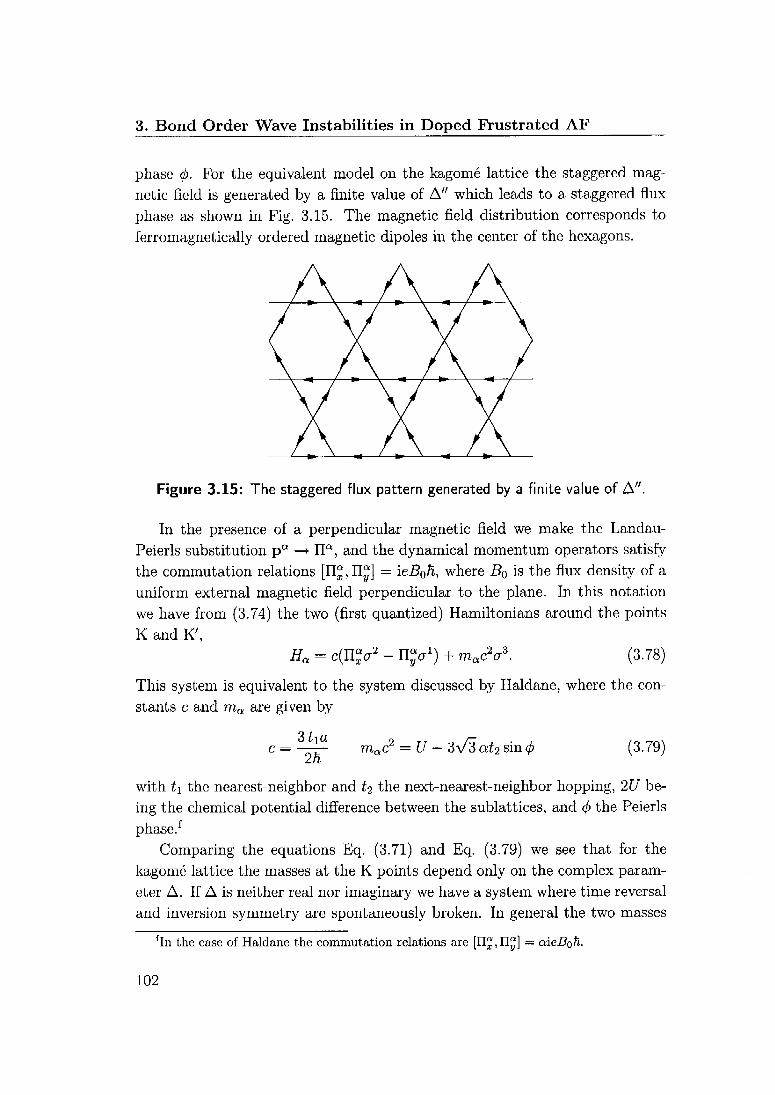
3. Bond Order Wave Instabilities in Doped Frustrated AF
phase (f). For the equivalent model on the kagomé lattice the staggered mag¬
netic field is generated by a finite value of A" which leads to a staggered flux
phase as shown in Fig. 3.15. The magnetic field distribution corresponds to
ferromagnctically ordered magnetic dipoles in the center of the hexagons.
Figure 3.15: The staggered flux pattern generated by a finite value of A".
In the presence of a perpendicular magnetic field we make the Landau-
Peierls substitution pa —> na, and the dynamical momentum operators satisfy
the commutation relations [n£, n^] — \eBQh, where B0 is the flux density of a
uniform external magnetic field perpendicular to the plane. In this notation
we have from (3.74) the two (first quantized) Hamiltonians around the points
K and K',
Ha - c(Uy2 - Tl^a1) + mac2a3. (3.78)
This system is equivalent to the system discussed by Haldane, where the con¬
stants c and ma are given by
Q J.
c = —~ mac2 = U-3*33 at2 sin 0 (3.79)ZilL
with ti the nearest-neighbor and t2 the next-nearest-neighbor hopping, 2U be¬
ing the chemical potential difference between the sublattices, and 4> the Peierls
phase.f
Comparing the equations Eq. (3.71) and Eq. (3.79) we sec that for the
kagomc lattice the masses at the K points depend only on the complex param¬
eter A. If A is neither real nor imaginary we have a system where time reversal
and inversion symmetry arc spontaneously broken. In general the two masses
In the case of Haldane the commutation relations are [11^,11] = aieB0ti.
102
3.8. The Dirac points of the kagomé lattice
ma are not equal and for A"/A = ±\/3 we have a finite gap at one K point
whereas the other K point is a gapless Dirac point. It is therefore possible
to avoid the fermion doubling by simultaneously breaking time reversal and
inversion symmetry.5
The following discussion of the zero-field quantum Hall phases on the kagomé
lattice follows closely the analogous discussion of Haldane for the honeycomb
lattice [5]. In the presence of a uniform perpendicular magnetic field with flux
density B0 the spectra of the Hamiltonians of Eq. (3.78) change and relativistic
Landau levels are obtained [116]
Ean± = ±[(mac2)2 + nh\eB0\c2]i (n > 1), (3.80)
Eao = mJac2sign(eB0). (3.81)
Note, that the spectrum of a single species of fermions is not particle-hole
symmetric, as the zeroth Landau level (3.81) has no counterpart. In the time
reversal symmetric case, we have m+ ——m_ and the particle hole symmetry
of the total spectrum is restored. Furthermore, the spectrum is invariant under
B0 —> —B0 and the quantized Hall conductance, axy, is zero. If the masses ma
have opposite signs, there is exactly one of the two Landau level, Eafi, filled.
If one of the masses ma changes sign, an additional Landau level is filled or
emptied.
In general the additional charge density in the ground state with respect to
the time-reversal symmetric situation is given byh
Aa = (e2BQ/h) ^ sign(mQ)/2. (3.82)a
The value of the Hall conductance can be obtained from the thermodynamic
relation axy — da/dB0\ßiT, where a is the 2D electric charge density. From
Eq. (3.82) we get therefore the quantized Hall conductance uxy — ue2/h with
v = X^asign(ma)/2. Note, that we get a result that can be evaluated for
B0 — 0, i.e., we obtain an integer quantum Hall effect without applying an
external magnetic field. The phase diagram depends only on the phase of A, 4>
and is shown in Fig. 3.16. The system posses an intrinsic chirality that leads
to the non-vanishing quantized Hall conductance axy even without applied
external magnetic field.
sAs long as only time-reversal or inversion symmetry is broken, the dispersion is still
invariant under k —> —k.
hWe choose the electronic charge e < 0.
103

3. Bond Order Wave Instabilities in Doped Frustrated AF
V
-1
-2jt/3 -n/3 jt/3 2jt/3
1
K<t>
Figure 3.16: The phase diagram as a function of 4> which is the phase of A.
The zero-field Hall conductance at zero temperature is given by axy — ve2jh and
v = Ha sign(ma)/2.
It is interesting to look at the degenerate states at the points K and K' in
more detail. From Eq. (3.72) and Eq. (3.60) one can see that it is convenient
to use the notation
4lo> = |v,o) *i|o) = |a,o)
4lo) = |a,o) 4'lo) = |v,o)' (3.83)
where in the state | V, Ö) the phase on each V triangle increases by 27r/3 along
each bond in the clockwise direction, whereas the phase is constant on the A
triangles. In the state |A,0) the phase on each A triangle increases by 27r/3
along each bond in the anti-clockwise direction whereas the phase is constant
on the V triangles and analogously for the other states. For the operators
Hy = - XXm+lCr,m-i + h-C-
rm
" A—
~
2^ Cr,m+lCr+am,m-l + n-C')
(3.84)
where HA contains the hopping processes on the A triangles and H7 the pro¬
cesses on the V triangle. For A — 0 we have
(A, Ü|#V|A, O) - -2, (A, 0|#a|A, Ö) = 1. (3.85)
For the other states hold analog expressions. The effect of the inversion sym-
104

3.9. Discussion and conclusion
metry X and the time reversal symmetry T on these states is given by
J|A,0) - |V,0)
J|A,Ö) = |V,0)
Z|V,0) = |A,Ö)
X|V,0) - |A,Ö)
From this follows, that if time reversal symmetry is broken, states with the
same chirality are degenerate, but if the inversion symmetry is broken, states
with the same triangles are degenerate. The situation where the states with the
same chirality are above the gap can not be changed into the situation where
the states with the same triangles are above the gap, without closing at least
one gap. The closing of the gap marks the phase transition between phases
with different quantum Hall conductance. In Fig. 3.17 the amplitudes of the
state | A, O) are drawn. For the kagomé strip we also have the four degenerate
states of Eq. (3.83). Note,that in this case to outer triangles have been turned
down by the periodic boundary conditions and therefore we have seemingly
triangles with both chiralities in the state |A, O)-
Figure 3.17: The amplitudes of the state | A, O) are drawn on the kagomé lattice
and on the kagomé strip where the triangles on every second rung are turned down.
3.9 Discussion and conclusion
In summary we have studied the occurrence of a bond order wave instabil¬
ity in the four different bisimplex lattices shown in Fig. 3.1. We provided
evidence that this instability occurs quite generally in all four lattices at the
fractional filling of one electron per simplex (two electrons per up-simplex),
T|A,0)
T]A,Ü)
T|V,0)
TIV.O)
|a,o)
|a,o)
|V,Ö)
|v,ü)
(3.86)
105

3. Bond Order Wave Instabilities in Doped Frustrated AF
if the correlations (i.e., nearest-neighbor repulsion and/or antiferromagnetic
nearest-neighbor exchange) are strong enough.
In weak coupling the physical properties of the system are dominated by
the dimensionality of the lattice, by its fermiology and by the density of states
at the Fermi energy. We show that in the intermediate coupling regime, where
the kinetic and the interaction energies are comparable, at the filling with
two electrons per up-simplex, the physical properties of these highly frustrated
lattices are dominated by local states on the simplex. The bipartite and corner-
sharing arrangement of the simplices allows the creation of isolated or only
weakly interacting simplices with low-energy by spontaneously breaking the
inversion symmetry. This knowledge provides a good starting point for series
expansions or further CORE calculations.
The magnetic interaction and the chosen sign of the dispersion leads to
a tendency to form nearest-neighbor singlets and nearest-neighbor repulsion
leads to a tendency to avoid configurations with more than two electrons per
simplex. If the underlying lattice is bipartite the system finds a way to satisfy
both tendencies simultaneously by localizing singlets on every second simplex.
This localization leads only to a partial loss of the kinetic energy, because the
singlets can still delocalize within the simplex. It is the cooperation between the
kinetic and the interaction energy which stabilizes the bond order wave state.
Note, that the bond order wave instability does not lead to an inhomogeneous
charge distribution on the lattice.
The bond order wave states, which we find on the different lattices, pro¬
vide a natural generalization of the well-known valence bond solid states (e.g.,dimerizcd phases, plaquette phases) found in many frustrated spin models to
situations away from half-filling where a description in terms of spin variables
only breaks down. The density is still a rational fraction, but n = 2/3 in
the kagomé and kagomé strip case while n = 1/2 in the pyrochlore and the
checkerboard case. Approximately these states are direct products of singlets
on triangles or tetrahedra, similar to the conventional picture of a dimerized
phase. In contrast to the phases at n — 1 the present instability involves a
cooperative effect of both magnetic exchange and kinetic energy.
An interesting task is to study the properties of a lightly doped bond order
wave phase. It can be assumed that the bond order wave order parameter
decreases rather quickly with doping. However, it is conceivable that away
from the commensurate filling the bond order wave order parameter coexists
with a small superconducting order parameter. This phase would at the same
106

3.9. Discussion and conclusion
time break lattice symmetries and the U(l) gauge symmetry and would be
therefore similar to a supersolid.
In general, we conclude that the bond order wave instability in the four
lattices of Fig. 3.1 occurs for physically reasonable models and interaction pa¬
rameters. Our study shows that doping frustrated spin models can lead to new
phases and hopefully contributes to a further understanding of the interplay
of frustrated magnetic fluctuations and itinerant charge carriers, which play a
role for example in the unconventional heavy Fermion material L1V2O4 [91, 92]
or in Nai.Co02.
107

Seite Leer /
Blank leaf

Chapter 4
Inhomogeneously Doped
t-J Ladder and Bilayer Systems
4.1 Introduction
Doped spin liquids have been an important subject of condensed matter re¬
search for the last two decades, mainly due to their possible relevance to the
(cuprate) high-temperature superconductors (HTSC)[117, 118]. Although it is
still not understood how high-temperature superconductivity emerges from an
antiferromagnetic Mott-insulator upon carrier doping, there is broad consen¬
sus that an intermediate pseudogap phase plays a crucial role in understanding
both the exotic normal and superconducting properties of these materials [119].
Many proposals concerning the nature of the pseudogap phase have been put
forward. One candidate for the pseudogap phase is the resonating valence bond
state (RVB), which describes strongly fluctuating short-ranged spin singlets
[117]. While the relevance of this state to the quasi-two-dimensional HTSC is
still under debate, it is realized in specially designed lattice structures [120],Of particular interest are systems with ladder-shaped crystal structures, which
are realized in various transition metal oxide compounds [1, 121].
Undoped, these ladder-systems are Mott-insulators and well described by
quantum spin-1/2 Heisenberg models. For the two-leg ladder the ground state
is an RVB-like state displaying short-ranged spin-singlet correlations with spin-
singlet dimcrs on the rungs dominating over those along the legs. This con¬
stitutes a spin liquid with a finite energy gap to the lowest spin excitations.
Furthermore, it was proposed that such a system would exhibit superconduc-
109

4. Inhomogeneously Doped t-J Ladder and Bilayer Systems
tivity upon hole-doping [122, 123]. Various theoretical approaches confirmed
a strong tendency towards formation of Cooper pairs with phase properties
reminding of the dx2_y2-wave channel of the two-dimensional HTSC [124-127].
The theoretical proposals were followed by an intense material research
attempting to dope holes into a variety of known insulating copper-oxide com¬
pounds displaying ladder structures [128]. Materials under consideration are
SrCu203, CaCu203, LaCu02.5, and Sr^CWO^. Doping these compounds
is intrinsically difficult because of chemical instabilities, and carrier localiza¬
tion effects may inhibit the desired metallic behavior. Nevertheless, the search
for superconductivity has been successful in the compound Sr14_a;CaxCu2/i04i
which contains layers of ladders alternating with layers of single chains [129].In this material Tc rises up to about 12 K under high pressure, which appar¬
ently leads to a transfer of charge carriers from the chains onto the ladders.
However, a detailed understanding of this system under high pressure has not
been reached yet. A well-controlled and less invasive way of doping a ladder
compound is thus highly desirable.
Hole and electron doping by means of field effect devices induces mobile
charge carriers into the originally insulating material using a large gate voltage.
This method would be ideal for doping quasi one- and two-dimensional systems,
since the induced charge is confined to the outer-most layer of the compound,
closest to the gate.
An alternative technique of tunable doping has been achieved using het-
erostructures of layered materials such as high-Tc-cuprates combined with fer-
roelectrics like Pb(Zr,Ti)03 [130-132].For ladder systems the most natural choice for this type of doping control
is a film in which the ladder planes lie parallel to the gate or the ferroelectric,
so that the carriers enter the ladders uniformly. However, in the compound
LaCu02.5 the ladders are not parallel to each other, but exhibit a staggering
[133]. Consequently, in a field effect device the ladders would be inhomoge¬
neously doped in the sense that the chemical potential on the two legs would
be different. Similarly, a variable orientation of the dipolar moments of the
ferroelectric can lead to inhomogeneous doping.
For bilayer compounds like YBa2Cu307_6 the symmetry between the layers
would be broken by the presence of the electric field, leading to a difference
between the chemical potentials of the layers and consequently to an inhomo¬
geneous doping concentration in the two layers.
These non-volatile techniques of tunable doping may allow for a detailed
110

4.2. Strong rung coupling limit
comparison between experiment and theory in these low-dimensional struc¬
tures.
In this chapter we analyze the evolution of the superconducting state un¬
der such doping circumstances. Our analytical and numerical analysis of the
ID system shows that non-uniform doping is harmful to the superconducting
state of the two-leg ladder. The strong pairing correlations on the rung are
suppressed by the application of the electric field. While for small Ap the
ladder remains superconducting, the pairing is suppressed upon increasing A^,,
and depending on the doping level new phases with reduced, and eventually
without superconductivity appear.
The mean-field analysis for the bilayer leads to similar results for the s-wave
superconducting phase, which has strong inter-plane pairing correlations. In
contrast to the ladder case, however, there exists also a d-wave superconducting
phase for the bilayer, which is less affected by the interplane potential difference.
This chapter is organized according to the used analytical and numerical
methods. In this way we study various aspects of the problem within different
approximative schemes. In the following section a qualitative argument for the
limited stability of the superconducting state upon inhomogeneous doping is
presented. In Sec. 4.3 a discussion of numerical exact diagonalization results
is given for the charge correlations of two holes in ladders with up to 22 sites.
Then, in Sec. 4.4 we apply renormalization group (RG) and bosonization meth¬
ods to derive the phase diagram of the weakly interacting Hubbard model in
the inhomogeneously doped case. In Sec. 4.5 we consider a mean-field treat¬
ment of the t-J model based on the spinon-holon decoupling scheme. With this
method we study both the inhomogeneously doped ladder and the bilayer sys¬
tem. Finally, we summarize and conclude in Sec. 4.7 and draw a unified picture
of the behavior of inhomogeneously doped two-leg ladder and bilayer systems
by combining the results from the earlier sections. The results for the two-leg
ladder are published in Ref. [134]. The ED data (Sec. 4.3) were obtained from
Andreas Läuchli and the RG calculations (Sec. 4.4) were performed by Stefan
Wessel in the framework of a collaboration on Ref. [134].
4.2 Strong rung coupling limit
The influence of a difference in the chemical potential on the pairing state
of the two-leg ladder or the bilayer can be illustrated by a simple qualitative
argument for the t-J model. Consider the two-leg ladder with electrons moving
111
4. Inhomogeneously Doped t-J Ladder and Bilayer Systems
along the legs and rungs with hopping matrix elements t and t', respectively,
and nearest-neighbor spin exchange with exchange constants J and J'. The
Hamiltonian of the t-J model for the two-leg ladder then reads
jas
+J 2_^ ( Sja • Sj+i)0 - -njanj+ita Jja
" /^^njaa. (4.1)jas
The operator cjas (cjas) creates (annihilates) an electron with spin s on site
(j,a), where j labels the rungs and a — 1,2 the legs. The electron number
operators are defined as n-as — cjasc-os, and nja — J2Snjas- The spin operators
are
^ja 9 ^ Cj'os °"ss' C?w' ^ '
where era, a = 1, 2, 3, are the Pauli matrices. The constraint of excluded double
occupancy is enforced by the projection operator
^=n(i-n^T"i-i)- (4-3)ja
In the last line of Eq. (4.1) different chemical potentials on the two legs, pa,
describe an inhomogeneous doping of the system. Throughout this paper we
assume Ap — pi— p2 > 0 and refer to the leg with a — 1 (a — 2) as the upper
(lower) leg. Furthermore, the overall doping concentration 8 — 1 — n fixes the
average chemical potential p — (pi + p2)/2.The phases of the t-J model on the two-leg ladder for Ap — 0 are well
characterized [135]. At half-filling (8 — 0) with one electron per site the ladder
is a (Mott-) insulating spin liquid. Upon removal of electrons, i.e., doping of
holes, mobile carriers appear, resulting in a Luther-Emery liquid with gapless
charge modes and gapped spin excitations. Furthermore, the gapless charge
mode exhibits dominant superconducting correlations with a rf-wave-like phase
structure.
112
4.2. Strong rung coupling limit
We now discuss the effect of inhomogeneous doping on this superconducting
state, described by Ap > 0. For many aspects of ladder systems the limit of
strong rung-coupling gives useful insights into their basic properties. Therefore
we first consider the Hamiltonian (4.1) in the limit J',t' 2> J, t. Neglecting
the coupling along the legs entirely the undoped system corresponds to a chain
of decoupled rungs and the ground state becomes a product state of dimer
spin-singlets on the rungs. Note, that this product state of singlets can also be
written as a (Cooper) pair wave function in the form [118]
11;* (»«»«-<Mi) l°> <44>j
where the operator fcj, (at,) creates a bonding (antibonding) single-particle
state with spin s on the rung j. The different sign for the pairs with differ¬
ent transverse momentum already suggests the appearance of unconventional
superconductivity upon doping. In fact we will find in the mean-field calcula¬
tions of Sec. 4.5 that the pairing amplitudes on the rung and on the legs (layers)do have opposite signs. If the two-leg ladder is viewed as cut of finite width
through the square lattice and if the transverse momentum is denoted by ky,
the sign change between the Cooper pairs with ky — 0 and ky — n reminds of
a superconducting state with dx2 „y2-symmetry.
Furthermore, the lowest spin excitation corresponds to exciting one rung-
singlet to a triplet, at an energy expense of ,/'. The superconducting state,
i.e., Cooper pairing, in the doped spin liquid is inferred from the fact that
two doped holes rather reside on a single rung rather than to separate onto
two rungs. This is the case if the dominant energy scale is the spin exchange
interaction, J'. Then the cost of breaking two spin singlets is larger than the
gain of kinetic energy from separating the two holes. Namely, for two holes on
a single rung the energy is
E2h = 3'- 2p, (4.5)
while for a single hole
Elb = 3'-ß- \^4(t')2 + Ap2. (4.6)
Pairing on a rung is favored, if
2Elh - E2h = J'- V4(i')2 + Ap2 > 0, (4.7)
113
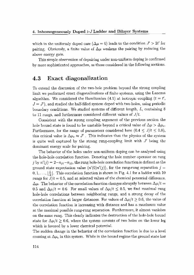
4. Inhomogeneously Doped t-J Ladder and Bilayer Systems
which in the uniformly doped case (Ap = 0) leads to the condition J' > 2t' for
pairing. Obviously, a finite value of Ap weakens the pairing by reducing the
above energy gain.
This simple observation of depairing under non-uniform doping is confirmed
by more sophisticated approaches, as those considered in the following sections.
4.3 Exact diagonalization
To extend the discussion of the two-hole problem beyond the strong coupling
limit we performed exact diagonalizations of finite systems, using the Lanczos
algorithm. We considered the Hamiltonian (4.1) at isotropic coupling (t — t',
J — J'), and studied the half-filled system doped with two holes, using periodic
boundary conditions. We studied systems of different length, L, containing 8
to 11 rungs, and furthermore considered different values of J/t.Consistent with the strong coupling argument of the previous section the
hole bound state is found to be unstable beyond a critical value of Ap > Apc.
Furthermore, for the range of parameters considered here (0.4 < J/t < 0.8),this critical value is Apc ~ J'
.This indicates that the physics of the system
is quite well captured by the strong rung-coupling limit with J' being the
dominant energy scale for pairing.
The behavior of the holes under non-uniform doping can be analyzed using
the hole-hole correlation function. Denoting the hole number operator on rung
j by n'(j) — 2—riji—nj2, the rung hole-hole correlation function is defined as the
ground state expectation value (n'(O)n'(j)), for the rung-rung separation j —
0,1,..., LfJ •This correlation function is shown in Fig. 4.1 for a ladder with 10
rungs for J/t = 0.5, and at selected values of the chemical potential difference,
Ap. The behavior of the correlation function changes abruptly between Ap/t —
0.5 and Ap/t — 0.6. For small values of Ap/t < 0.5, we find maximal rung
hole-hole correlations between neighboring rungs, and a strong decay of the
correlation function at larger distances. For values of Ap/t > 0.6, the value of
the correlation function is increasing with distance and has a maximum value
at the maximal possible rung-rung separation. Furthermore, it almost vanishes
on the same rung. This clearly indicates the destruction of the hole-hole bound
state for Ap/t > 0.6, where the system consists of two holes on the lower leg
which is favored by a lower chemical potential.
The sudden change in the behavior of the correlation function is due to a level
crossing at Apc in this system. While in the bound regime the ground state has
114
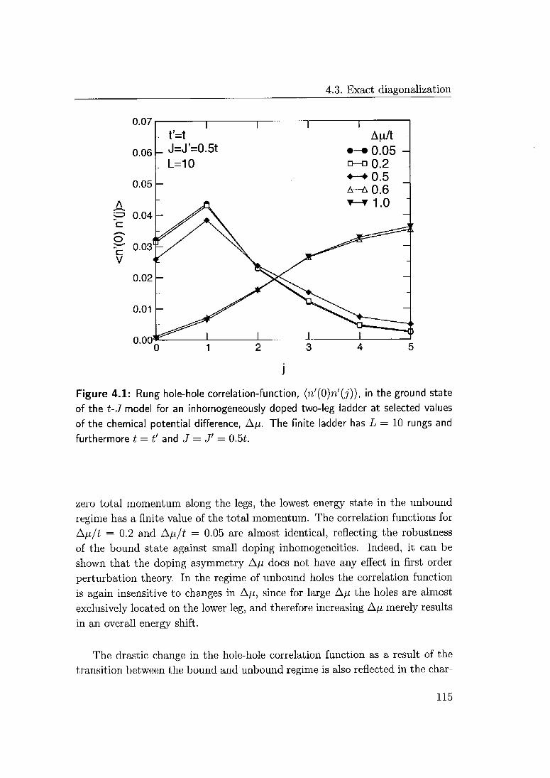
4.3. Exact diagonalization
S"c
S;tv
J
Figure 4.1: Rung hole-hole correlation-function, (n'(0)n'(j)), in the ground state
of the t-3 model for an inhomogeneously doped two-leg ladder at selected values
of the chemical potential difference, Ap. The finite ladder has L — 10 rungs and
furthermore t = t' and 3 = 3' — 0.5t.
zero total momentum along the legs, the lowest energy state in the unbound
regime has a finite value of the total momentum. The correlation functions for
Ap/t — 0.2 and Ap/t — 0.05 are almost identical, reflecting the robustness
of the bound state against small doping inhomogeneities. Indeed, it can be
shown that the doping asymmetry Ap does not have any effect in first order
perturbation theory. In the regime of unbound holes the correlation function
is again insensitive to changes in Ap, since for large Ap the holes are almost
exclusively located on the lower leg, and therefore increasing Ap merely results
in an overall energy shift.
The drastic change in the hole-hole correlation function as a result of the
transition between the bound and unbound regime is also reflected in the char-
115

4. Inhomogeneously Doped t-3 Ladder and Bilayer Systems
6.0
5.0
4.0
3.0
2.0
1.0
—T 1
t'=t
J=J'=0.5t
L
10
D D 8
-• • • d>
D O D []
0.0 0.2 0.4 0.6 0.8 1.0
Ajl/t
Figure 4.2: Characteristic hole-hole separation length, £, in the ground state of
the t-3 model for an inhomogeneously doped two-leg ladder as a function of the
difference in the chemical potential, Ap, for L ~ 8 (circles), and L — 10 (squares).
Furthermore, t' = t and 3 = 3' — 0.51.
acteristic hole-hole separation length, £, defined by
l#l-i
? = }/ E 32(A0)n'U))t (4.8)
J"=-L#J
where A" is a normalization factor given by N — J2j(n'(Q)n'(j)). In Fig. 4.2, this
separation length is plotted as a function of Ap for two different systems with an
even number of rungs, L — 8 and L = 10.a For both systems the characteristic
hole-hole separation length jumps discontinuously at a critical value of Apc rj
3'. Furthermore, in the bound regime, i.e., for Ap < Apc, finite size effects
in this quantity are rather small already for the system sizes considered here.
In this regime the holes are bound, and the rung hole-hole correlation decays
aThe system with L = 9 also exhibits a clear tendency towards unbinding, however no
level crossing but rather a crossover between the two regimes occurs. For L = 11 a level
crossing is found, with the total momentum jumping from 0 to a finite value near 0, whereas
in the even systems the total momentum changes from 0 to a value near n. In view of these
odd-even effect, we restrict the discussion to finite ladders with an even number of rungs.
116

4.4. Renormalization group
exponentially. Therefore, the bound pair wave function extends over only a few
rungs. In the unbound regime, however, the two holes tend to separate onto
the lower leg, and therefore £ grows with increasing system size.
The above numerical analysis demonstrates that non-uniform doping, by
confining the mobile carriers onto one of the legs, is harmful to pairing. Further¬
more, the inter-leg exchange interaction plays the important role of stabilizing
the bound hole pair state. While the finite ladders considered in this section
may be viewed as systems with a doping concentration of roughly 8 ~ 0.1,
different approaches are needed to analyze the finite-doping regime beyond the
two-hole problem. These will be presented in the following sections.
4.4 Renormalization group
In order to complement the analysis of the t-3 model, in this section we consider
the weakly interacting Hubbard model on a two-leg ladder. A renormalization
group (RG) treatment supplemented by Abelian bosonization allows a detailed
analysis of the phase diagram in the weakly interacting limit and a charac¬
terization of the various phases in terms of the low-energy modes. We follow
an approach established on standard two- and N-\eg ladder systems (i.e., for
Ap = 0) [16, 126, 136, 137].In the current case of an inhomogeneously doped two-leg ladder we consider
the weak repulsive limit, 0 < U -C t, t' of the Hubbard model,
H = -*Z(cî«ci+i,« + h-c-)-*'E(cîi-cja- + h-c-) (49)jas js
+^Z-e CJalCjaîCjalCjal
~
/_^ ^a CjasCjasija jas
with the same notations as is Sec. 4.2. The quadratic part of the Hamil¬
tonian (4.9), i.e., Eq. (4.9) with (7 = 0, can be decoupled via a canonical
transformation
t /lTA^t ll±Ap/D {
aj,i(2),s~]j 2 j2s V 2 ?ls' l '
where D = y/A(t')2 + Ap2. These rung operators interpolate smoothly be¬
tween the bonding and anti-bonding combinations at Ap = 0 and the original
fermions for Ap/t' —> oo, where d^as —> c]a,. In momentum space two bands
117
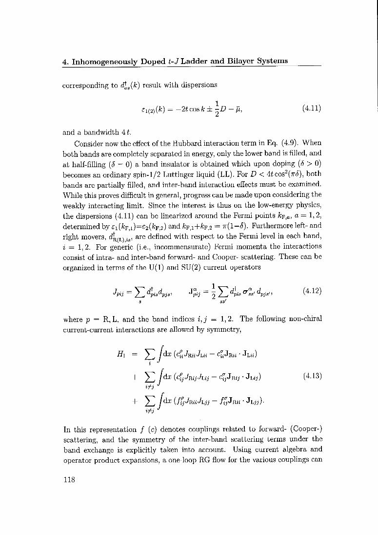
4. Inhomogeneously Doped t-3 Ladder and Bilayer Systems
corresponding to d\s(k) result with dispersions
ei(2)(A:) = -2tcosfc±-Z?-/i, (4.11)Zt
and a bandwidth 41.
Consider now the effect of the Hubbard interaction term in Eq. (4.9). When
both bands are completely separated in energy, only the lower band is filled, and
at half-filling (8 = 0) a band insulator is obtained which upon doping (8 > 0)
becomes an ordinary spin-1/2 Luttinger liquid (LL). For D < 4tcos2(7r5), both
bands arc partially filled, and inter-band interaction effects must be examined.
While this proves difficult in general, progress can be made upon considering the
weakly interacting limit. Since the interest is thus on the low-energy physics,
the dispersions (4.11) can be linearized around the Fermi points kF,a, a = 1,2,
determined by £i(kF,i)=e2(kF,2) and &f,i+&f,2 = n(l-8). Furthermore left- and
right movers, dLL) is,are defined with respect to the Fermi level in each band,
i = 1,2. For generic (i.e., incommensurate) Fermi momenta the interactions
consist of intra- and inter-band forward- and Cooper- scattering. These can be
organized in terms of the U(l) and SU(2) current operators
Jpij = /_^ dpisdpjs, Jpij — -
2_^ dpis crss/ dpjs,, (4.12)
s ss'
where p — R, L, and the band indices i,j = 1,2. The following non-chiral
current-current interactions are allowed by symmetry,
Hi = yj
jdx (eftJr„Jlü — CjjJmi • Jlü)i
J
+ Y fdx (4jJjJuj - c^JRij Juj) (4.13)&j
+ IC /dX (fijJRiihjJ ~ fijJRH ' JLij)-i+j
In this representation / (c) denotes couplings related to forward- (Cooper-)
scattering, and the symmetry of the inter-band scattering terms under the
band exchange is explicitly taken into account. Using current algebra and
operator product expansions, a one-loop RG flow for the various couplings can
118
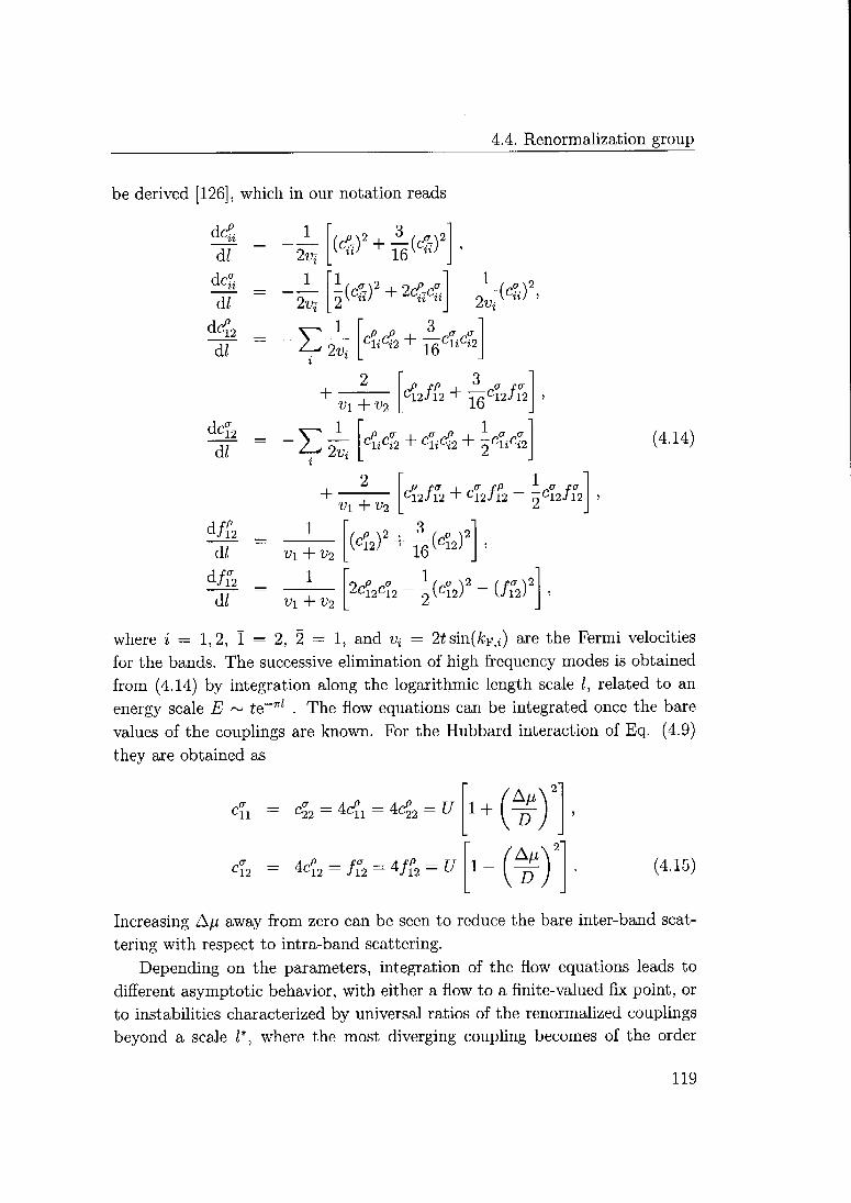
4.4. Renormalization group
be derived [126], which in our notation reads
dZ
d;
dcJ2dl
dra
dl
d/rkdl
dl
2vi
1
'2w
,a\2(4)2 + t^(4)
,a\2
2n
-E- ^li0^ + -<gLlil'i2
+
- -E
^1+^2
1
2w
C12/l2 + YgC12/l2
„<r „P1
+
clici2 + clici2 + 0clici2
C\2J12 + C12J\2 2°12-'12
(AAA)
Vi +V2
1
Vl + ^2
1
Ul + ^2
(cî.J' + ijjW,)'2c?,
1a\2
12^12 (C12)2 " (/f2)
where z = 1,2, I = 2, 2 = 1, and ^ — 2£sin(A;K,i) are the Fermi velocities
for the bands. The successive elimination of high frequency modes is obtained
from (4.14) by integration along the logarithmic length scale I, related to an
energy scale E ~ te~"*1.The flow equations can be integrated once the bare
values of the couplings are known. For the Hubbard interaction of Eq. (4.9)
they are obtained as
-il -22= 4c?! 4^2 U
cï2 = 4cf2 = ri2 = 4/f2 = U
1+[-lt)
£) (4.15)
Increasing Ap away from zero can be seen to reduce the bare inter-band scat¬
tering with respect to intra-band scattering.
Depending on the parameters, integration of the flow equations leads to
different asymptotic behavior, with either a flow to a finite-valued fix point, or
to instabilities characterized by universal ratios of the renormalized couplings
beyond a scale /*, where the most diverging coupling becomes of the order
119
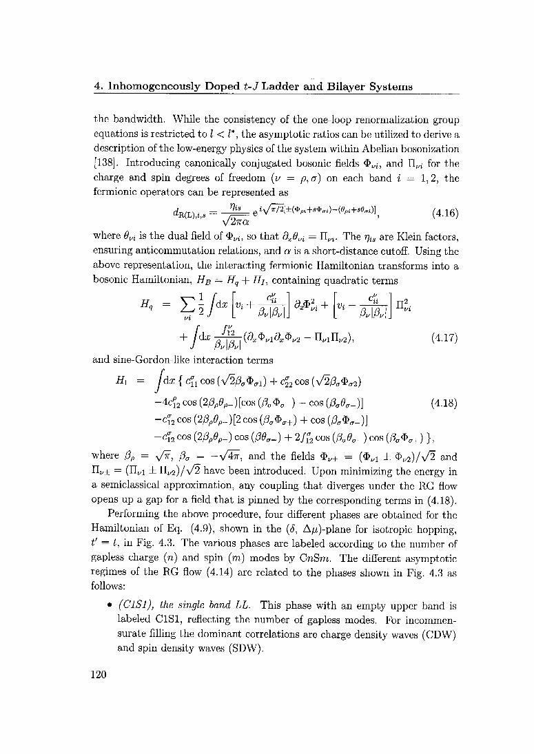
4. Inhomogeneously Doped t-3 Ladder and Bilayer Systems
the bandwidth. While the consistency of the one-loop renormalization group
equations is restricted to / < /*, the asymptotic ratios can be utilized to derive a
description of the low-energy physics of the system within Abelian bosonization
[138]. Introducing canonically conjugated bosonic fields $>Vi, and F[wi for the
charge and spin degrees of freedom (v — p, a) on each band i = 1,2, the
fermionic operators can be represented as
dR{L)ia = —^ e^T/w^..)-^^^ (4.i6)y/2na
where 6vi is the dual field of <&vi, so that dxdvi ~ Fiui. The riu are Klein factors,
ensuring anticommutation relations, and a is a short-distance cutoff. Using the
above representation, the interacting fermionic Hamiltonian transforms into a
bosonic Hamiltonian, HB = Hq -f- Hj, containing quadratic terms
1
», = £ dx Vi +ßAßA
dMi +
ßV\ßu\n
+ dx/l2
{dx$vidx$u2 - nvin„2), (4.17)ßu\ßu
and sine-Gordon-like interaction terms
Hi = [dx { C°n COS (V2ßa$al) +0^008 (V2ßa$a2)
-A(f12 cos (2ßp9p.)[cos (ßa$a-) ~ cos (AA-)] (4.18)
-C\2 COS {2ßp0pJ)[2 COS (ßa$a+) + COS (ßa$a-)}
-c\2 COS (2ßp9p.) COS (ßda-) + 2/f2 COS (ß„daJ) COS (&$,+) },
where ßp = ^/ïr, ßa = -y/Àlv, and the fields $„± = ($vl ± $I/2)/v/2 and
(n^i ± IiV2)/v2 have been introduced. Upon minimizing the energy inv±n
a semiclassical approximation, any coupling that diverges under the RG flow
opens up a gap for a field that is pinned by the corresponding terms in (4.18).Performing the above procedure, four different phases are obtained for the
Hamiltonian of Eq. (4.9), shown in the (<5, A/x)-plane for isotropic hopping,t' — t, in Fig. 4.3. The various phases arc labeled according to the number of
gapless charge (n) and spin (m) modes by CnSm. The different asymptotic
regimes of the RG flow (4.14) are related to the phases shown in Fig. 4.3 as
follows:
• (C1S1), the single band LL. This phase with an empty upper band is
labeled ClSl, reflecting the number of gapless modes. For incommen¬
surate filling the dominant correlations are charge density waves (CDW)and spin density waves (SDW).
120

4.4. Renormalization group
4.0
3.0
d—*
^ 2.0<
1.0
0.00.0 0.1 0.2 0.3 0.4 0.5
ô
Figure 4.3: Phase diagram of the inhomogeneously doped Hubbard model on
two-leg ladder in the weakly interacting limit, and for t' — t. The phases CrcSm
are labeled according to the number of gapless charge (n) and spin (m) modes.
Solid lines are phase boundaries. The dashed line indicates the crossover from a
region with dominant SC correlations in the lower and CDW and SDW correlations
in the upper band (C2S2.I), to a region dominated by CDW and SDW correlations
in both bands, for larger values of Ap (C2S2.II).
• (C2S2), the trivial fixed point. In this regime the couplings stay of order
U under the RG flow, or renormalize to zero. Therefore no gap opens in
this phase, labeled C2S2. Furthermore, the two partially filled bands are
decoupled in this regime. Standard LL theory [139] used to determine the
dominant correlations within each band, indicates a crossover between
two regions labeled C2S2.I, and C2S2.II respectively, cf. Fig. 4.3. The
dominant correlations in the C2S2.II regime are CDW and SDW within
both bands, whereas in the C2S2.I regime the lower band is dominated
by superconducting (SC) fluctuations.
• (C2S1), single-band superconductivity. Here, all couplings stay of the
121

4. Inhomogeneously Doped t-3 Ladder and Bilayer Systems
order of U or renormalize to zero, except for C22 ~ —v2. This results in
a pinning of the spin mode of the lower band, and the number of gapless
modes reduces to C2S1. SC correlations dominate the lower band, and
CDW and SDW correlations the upper band. Furthermore, inter-band
phase coherence is not established within this regime.
• (C1S0), inter-band superconductivity. In this regime the diverging cou¬
plings flow towards the asymptotic ratios
4cf2 - 8/f2 = c\2, cau fVl = c°22/v2. (4.19)
From the low-energy effective bosonic Hamiltonian two finite spin gaps
are obtained, and a pinning of the charge mode 8P- — 0, resulting in
phase coherence between the two bands. The number of gapless modes is
reduced to C1S0. The remaining total charge mode, ($p+, 0P+), is gaplessand exhibits dominant superconducting pairing correlations, with a sign
difference between the bands. This is usually referred to as the d-wave-like
superconducting phase of the two-leg ladder [126, 136].
The phase diagram in Fig. 4.3 confirms the results obtained along the line
Ap, = 0 [126, 136]. But it also indicates a limited stability of the various phasesfound at Ap = 0 under inhomogeneously doping of the ladder. Upon increas¬
ing Ap, superconductivity is gradually suppressed, with intermediate phases
showing residual superconducting fluctuations. Consider for example the low
doping region where inter-band d-wave superconductivity occurs for vanishing
Ap. While for small Ap > 0 rf-wave superconductivity sustains, inter-band
phase coherence is lost when Ap reaches a value of approximately 1.5t'. For
larger values of A^ intra-band superconductivity persists within the lower band
(which predominately projects onto the lower leg of the ladder). In the upper
band spin fluctuations have become gapless and SDW and CDW correlations
dominate. Further increase of Ap results in the suppression of all superconduct¬
ing correlations, giving rise to two-band LL behavior. In the weakly interactinglimit the upper band is depleted for Ap/t > 3.5, and a single-band LL, residing
mainly on the lower leg of the ladder, dominates the large-A/x regime. This
progressive reduction of superconducting pairing correlations is also observed
in the finite-temperature phase diagram. In Fig. 4.4 we show results for t' — t,
and Ap/t — 0.3 in the (8, T)-plane. From the renormalization of the energy
scale, E ~ te~nl, the logarithmic length scale of Eq. (4.14) can be related to a
temperature scale T — E ~ T0e~*1. While the phases of the system for T —v 0
122
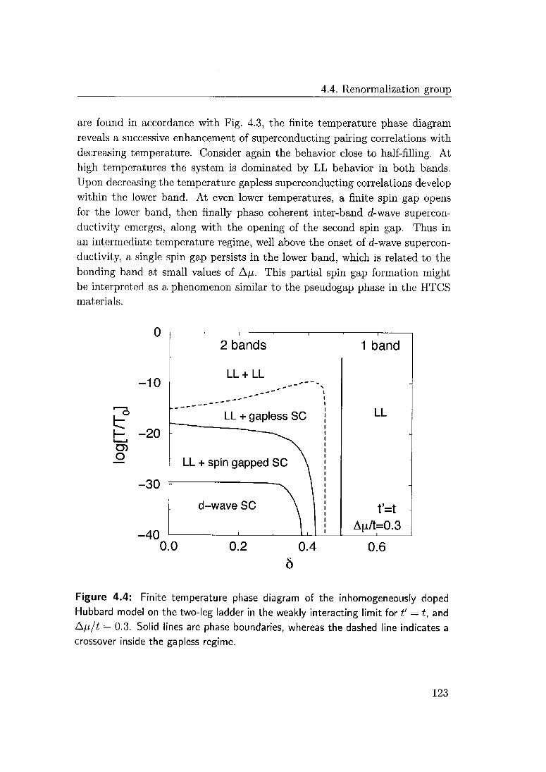
4.4. Renormalization group
are found in accordance with Fig. 4.3, the finite temperature phase diagramreveals a successive enhancement of superconducting pairing correlations with
decreasing temperature. Consider again the behavior close to half-filling. At
high temperatures the system is dominated by LL behavior in both bands.
Upon decreasing the temperature gapless superconducting correlations develop
within the lower band. At even lower temperatures, a finite spin gap opens
for the lower band, then finally phase coherent inter-band d-wave supercon¬
ductivity emerges, along with the opening of the second spin gap. Thus in
an intermediate temperature regime, well above the onset of d-wave supercon¬
ductivity, a single spin gap persists in the lower band, which is related to the
bonding band at small values of Ap. This partial spin gap formation mightbe interpreted as a phenomenon similar to the pseudogap phase in the HTCS
materials.
O
0
-10
-20
-30
-40
2 bands 1 band
LL + LL-
LL + gapless SC LL
LL + spin gapped SC \
t'=td-wave SC \
. ,
AuVt=0.3i
0.0 0.2 0.4
Ô
0.6
Figure 4.4: Finite temperature phase diagram of the inhomogeneously dopedHubbard model on the two-leg ladder in the weakly interacting limit for t' = t, and
Ap/t = 0.3. Solid lines are phase boundaries, whereas the dashed line indicates a
crossover inside the gapless regime.
123
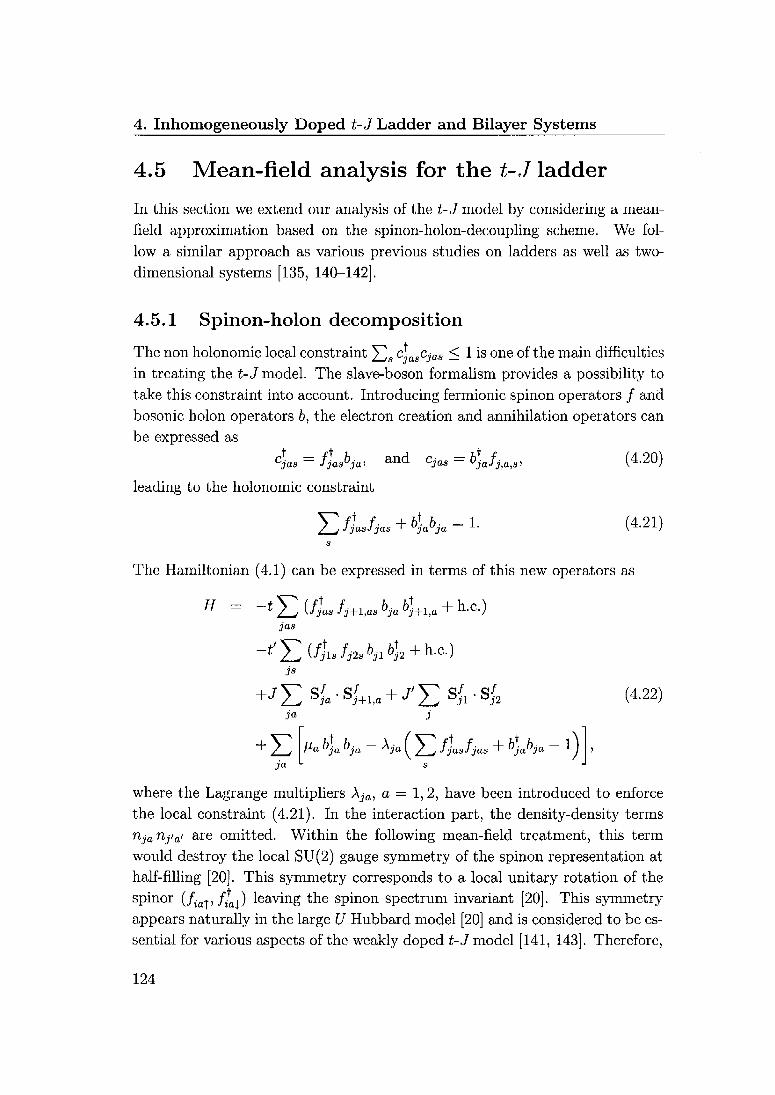
4. Inhomogeneously Doped t-3 Ladder and Bilayer Systems
4.5 Mean-field analysis for the t-J ladder
In this section we extend our analysis of the t-3 model by considering a mean-
field approximation based on the spinon-holon-decoupling scheme. We fol¬
low a similar approach as various previous studies on ladders as well as two-
dimensional systems [135, 140-142].
4.5.1 Spinon-holon decomposition
The non holonomic local constraint ^2S c,asCjas < 1 is one of the main difficulties
in treating the t-3 model. The slave-boson formalism provides a possibility to
take this constraint into account. Introducing fermionic spinon operators / and
bosonic holon operators b, the electron creation and annihilation operators can
be expressed as
c]a» = fja»bjv and CJ = h)afj,a,s> (4-20)
leading to the holonomic constraint
Ei^+fe-1- (4-21)s
The Hamiltonian (4.1) can be expressed in terms of this new operators as
H = -tJ2 (fjas fj+1,08 hja b}+l,a + ^-C.)jas
-t'UVhs^sbjib^ + h.c.)js
ja j
+ Y k 6Î- bJ* ~ V (E ftJjas+ blbJa ~ l)
ja"-
where the Lagrange multipliers Xja, a ~ 1,2, have been introduced to enforce
the local constraint (4.21). In the interaction part, the density-density terms
njanj'a' are omitted. Within the following mean-field treatment, this term
would destroy the local SU(2) gauge symmetry of the spinon representation at
half-filling [20]. This symmetry corresponds to a local unitary rotation of the
spinor (/ja|,//0i) leaving the spinon spectrum invariant [20]. This symmetry
appears naturally in the large U Hubbard model [20] and is considered to be es¬
sential for various aspects of the weakly doped t-3 model [141, 143]. Therefore,
124
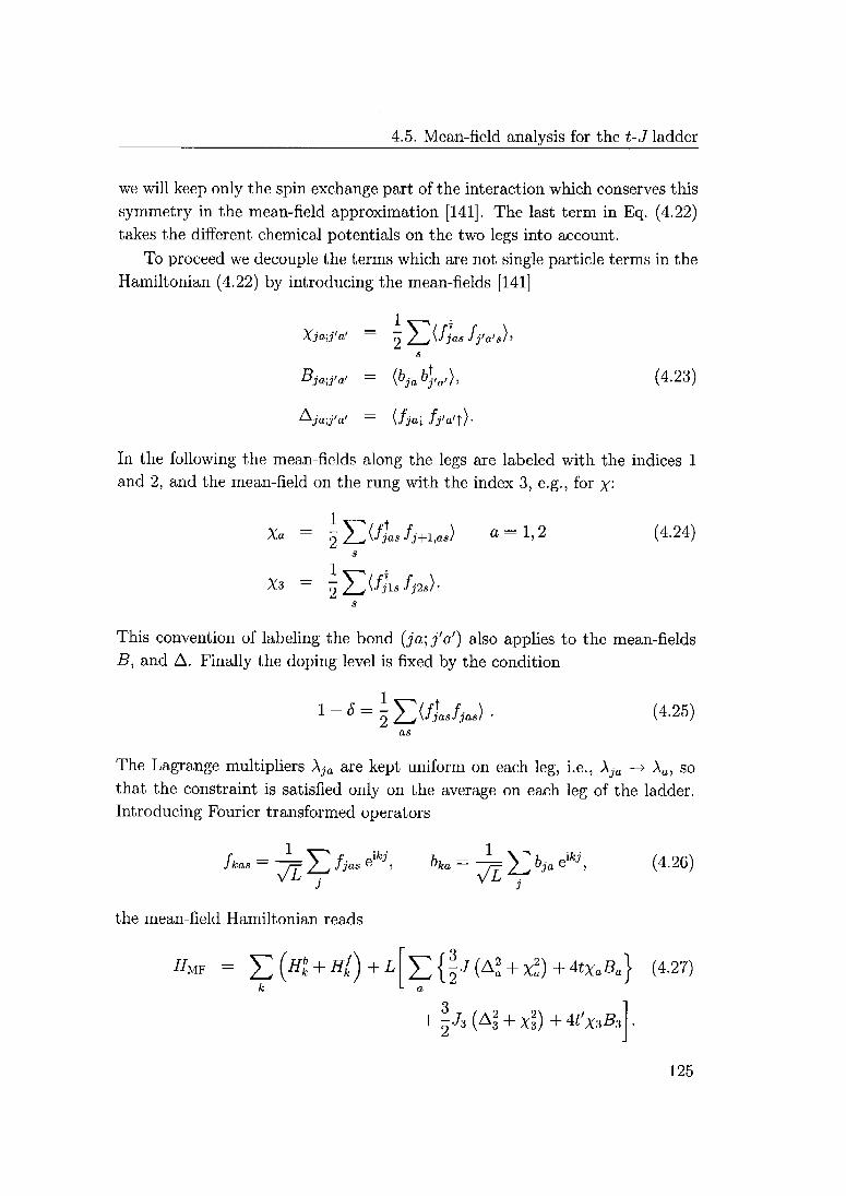
4.5. Mean-field analysis for the t-3 ladder
we will keep only the spin exchange part of the interaction which conserves this
symmetry in the mean-field approximation [141]. The last term in Eq. (4.22)takes the different chemical potentials on the two legs into account.
To proceed we decouple the terms which are not single particle terms in the
Hamiltonian (4.22) by introducing the mean-fields [141]
Xja;j'a' o / Nias Jj'a'sli
s
Bjaù'a' = (bjab],a,), (4.23)
Aja-j'a' = (fjalfj'a'])-
In the following the mean-fields along the legs are labeled with the indices 1
and 2, and the mean-field on the rung with the index 3, e.g., for x-
Xa = lYifjas /;+i,J «=1.2 (4-24)s
XS —
g / A-Mls Jj28/-
s
This convention of labeling the bond (ja; j'a') also applies to the mean-fields
B, and A. Finally the doping level is fixed by the condition
1 ~ S - lj2(fUjas) (4-25)
The Lagrange multipliers Xja are kept uniform on each leg, i.e., Xja —> Xa, so
that the constraint is satisfied only on the average on each leg of the ladder.
Introducing Fourier transformed operators
fkaS =~7£ E £«^ hk"=
7£E 6* C**' (426)j j
the mean-field Hamiltonian reads
#MF = Y(Hk + Hl)+L\T,{lJ(Aa + xl)+^XaBa} (4.27)k L
a
+ p3(Al + x23)+4t'x3B,
125

4. Inhomogeneously Doped t-3 Ladder and Bilayer Systems
The quadratic terms Hk and H[ are given by
6t
Hk -
fci
6tfc2
—At Xi cos k — Ai + pi
-2t'Xs
-2t'X3
-At X2 cos k — X2 + p2
H[
( f] \T r
Vfc2T
/-fcl|
\ /-fc2j /
& Afc
Afc —£fc
( fm \fk2\
/-fell
\f-k2iJ
where £&, and Äfc are the following 2x2 matrices
-Ai - (2tBl + §3xi) cos k -t'B36
!<to
t'B3 - 133X3 -A,(2tB2
2 + |^X2 cos k
Afc =— |JAi cos ft -|JA3
-FA3 —|JA2cos A;
The mean-fields are determined by self-consistently solving the single-particle
problem of #mf and calculating the corresponding expectation values accordingto Eqs. (4.23, 4.24).
Diagonalization of the bosonic part of the Hamiltonian yields two holon
bands. In the ground state of the system, the holons are assumed to Bose
condense into their lowest energy state [142]. Denoting the amplitudes of the
lowest holon state on the two legs by Aa, the bosonic bond mean-fields become
Ba - 28A2a,
B3 = 25^1,42.
a — 1, 2, (4.28)
The spinon part of the Hamiltonian can be diagonalized by a Bogoliubov trans¬
formation, from which the self-consistent equations for the mean-fields A and
X, and the Lagrange multipliers A are determined numerically. Furthermore we
define the BCS order parameters
^ja;j'a' :_ (Cja]cj'a'i/ (4.29)
^ (bjabj'a>)ifjaîfj'a'ni &ja;j'a'L±ja;j'a'
in terms of the holon and spinon mean-fields [140], For the BCS order param¬
eters we use the same bond labeling scheme as in Eq. (4.24).
126

4.5. Mean-field analysis for the t-J ladder
The redistribution of charge carriers due to the chemical potential difference
is implemented via the holon degrees of freedom as can be seen in the mean-
field Hamiltonian. In this way there is no effect at half-filling. Furthermore,
the constraint and the renormalization of the coupling constants induces a
non-trivial mutual feedback for the charge and spin degrees of freedom.
4.5.2 Mean-field results for the t-J ladder
Within the above mean-field description we are able to analyze the behavior
of the two-leg ladder for different values of the doping concentration, 8, and
chemical potential difference, Ap. In particular, we are interested in the BCS
order parameters as the indication for Cooper paring. In the following the
parameters of the t-J model are fixed to isotropic coupling with t' = t and J' =
J = 0.51. Furthermore, we restrict ourselves to the low doping region 8 < 0.25,
where the above spinon-holon decomposition is expected to be qualitativelyreliable [140].
0.02
0.01
0.00
^-0.01
-0.02
-0.03
0.3
DÜ 0.2
0.1
0.00.0 1.0 2.0 0.0 1.0 2.0 3.0
A[X Au.
Figure 4.5: BCS mean-fields A', (a,b), and hole densities B, (c,d), of the t-
J model on a two-leg ladder as functions of the chemical potential difference, Ap,at constant 8 = 0.1 (a,c), and 8 = 0.2 (b,d). t' = t and J' = J = 0.51. The
values for the lower (upper) leg are plotted with solid (dotted-dashed) lines and the
BCS mean-field on the rungs with dashed lines.
127

4. Inhomogeneously Doped t-J Ladder and Bilayer Systems
0.3
0.2
0.1
0.00.0 1.0 2.0 3.0 4.0
Au/t
Figure 4.6: Spinon gap As of the t-J model on a two-leg ladder as a function of
the chemical potential difference Ap at constant hole doping 5 — 0.1 (solid line)and 8 — 0.2 (dashed line) for t' — t, J' — J — 0.51. The inset shows the gapless
spinon bands in the normal state at 8 — 0.2. Ap/t — 2.0.
For Ap — 0 our calculations agree well with the overall behavior obtained
from similar mean-field calculations using a Gutzwiller-typc renormalization
method [135]. While at half-filling (8 — 0) the BCS order parameters vanish,
they increase monotonically with hole doping away from half-filling. Their
values on the legs coincide (A[ — A2), whereas a phase shift of n exists relative
to the rung order parameter Ag, in analogy to the d-wave pairing symmetry on
the square lattice version of the doped t-J model.
In order to analyze the influence of a chemical potential difference between
the two legs on the Cooper pairing, we follow the behavior of the BCS mean-
fields A'123 upon increasing Ap > 0 for two fixed hole concentrations, 8 ~ 0.1
and 8 — 0.2, shown in Fig. 4.5 (a,b). In both cases the chemical potentialdifference leads to the reduction and eventual destruction of the BCS mean-
fields. However, there is a qualitative difference between the two doping levels.
For 8 — 0.1 a crossover from a strong to a weak superconducting regime occurs,
while no such regime change takes place for 8 = 0.2. The crossover at Ap ^ 0.61
in Fig. 4.5 (a) for 8 = 0.1 coincides with the almost complete hole-depletion
of the upper leg in Fig. 4.5 (c). This behavior can be understood by the
following properties of doped two-leg ladders. These systems constitute typical
1.0 -\
1 o.o - ^7^-~^\ -1.0 /
\ -2.0
\ °
^ \
\ ^
\
\
\
.1
0 0.5 1.0
k/jt
1.5
128

4.5. Mean-field analysis for the t-J ladder
3.0
2.0
3.
<
1.0
0.00.0 0.1 0.2
Ô
Figure 4.7: Low doping phase diagram of the inhomogeneously doped two-legladder in the mean-field approximation of the t-J model at t' = t and J' — J —
0.51. The BCS mean-fields vanish beyond the solid line. In the low doping region
the crossover regime connecting the <i-wave SC and a regime of reduced BCS
mean-fields is indicated as a shaded area.
examples where superconductivity originates from a doped RVB phase, which
is characterized within this mean-field approach by a finite gap in the spinon
spectrum [135]. Furthermore, this spinon gap decreases upon doping holes into
a half-filled two-leg ladder [135]. Within the mean-field approximation we can
obtain the spinon gap at finite values of Ap for the doping levels considered
above. In Fig. 4.6 the development of the spinon gap upon increasing the
chemical potential difference, Ap, is shown for both 8 = 0.1, and S = 0.2. In
either case does the imbalance in the distribution of holes between the two legslead to an additional reduction of the spinon gap. This behavior is expected
as the RVB phase in the ladder is dominated by the formation of rung singlet
pairs. Concentrating the holes onto a single leg destroys statistically more
rung singlets than distributing them equally among both legs. However, at
<!> — 0.1, a large spinon gap is found even for e.g., Ap/t — 2, where the upper
leg is almost completely depleted, as seen in Fig. 4.5 (c). Although the holes
are already strongly concentrated onto the lower leg, the spinon gap is not
destroyed until Ap becomes as large as Apc m 2.61. Along with the RVB state,
(i-wave superconductivity thus prevails up to this critical value of A/ic, as seen
129
4. Inhomogeneously Doped t-J Ladder and Bilayer Systems
in Fig. 4.5 (a). For the larger doping of 8 = 0.2 however, concentrating the holes
onto the lower leg suppresses the spinon gap completely, thereby destroying the
RVB state. This follows from a comparison of the behavior of the spinon gap
in Fig. 4.6 with the corresponding behavior of the charge distribution shown in
Fig. 4.5 (d). Along with the spinon gap the superconducting state disappears
already at Apc m 1.5 t. However, the chemical potential difference which is
necessary to pull the holes onto the lower leg increases upon increasing the
hole doping level.
The resulting phase diagram in Fig. 4.7 displays a peculiar structure. For
low-doping concentrations 8 < 0.15 we observe two regimes, strong and weak
superconductivity, separated by a broad crossover. The crossover region is
characterized by the depletion of holes from the upper leg. For larger doping
8 > 0.15 only the regime of strong superconductivity remains, and the RVB
state is destroyed once the holes are sufficiently unequal distributed among the
two legs. The mean-field solution suggests that there exists a critical doping
8C « 0.08 below which the superconducting state along with the RVB spin
liquid state remains stable for all Ap.
Within the mean-field approximation the non-superconducting phase ap¬
pears to consist of two independent subsystems. This can be referred from
the inset of Fig. 4.6, which displays the gapless spinon bands at 8 = 0.2
and Ap/t — 2.0, well inside the normal phase. The spectrum consists of the
spinon bands of a spin-1/2 antiferromagnetic Heisenberg chain, with nodes at
k — ±7r/2, and two additional bands, with nodes at kF — ±7r/2(l — 28). These
nodes correspond to those of a single chain Luttinger liquid. The system in the
normal state therefore appears to be separated in a t-J chain with hole doping
28, having the properties of a Luttinger liquid, and a spin-1/2 antiferromag¬
netic Heisenberg chain. Furthermore, gapless charge excitations only exist for
the Luttinger liquid. This complete separation is likely an artifact of the mean-
field approximation, as in the strong rung coupling limit J' S> J the system is
obviously a single chain Luttinger liquid.
The mean-field description of the t-J ladder is in qualitative agreement with
the numerical result of Sec. 4.3 and with the the analysis of the weak-couplingHubbard model of the previous section. In the following section we apply the
same mean-field formalism for the t-J model to an inhomogeneously doped
bilayer.
130
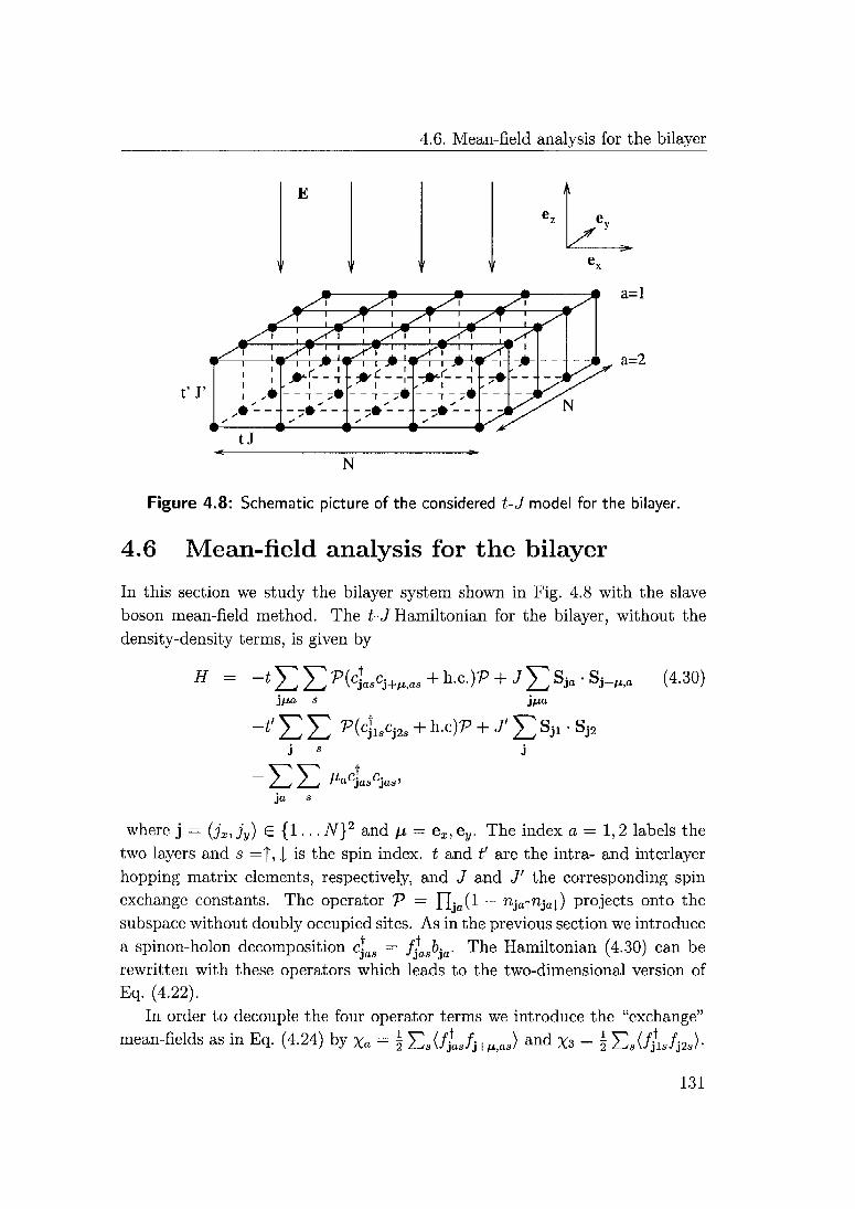
4.6. Mean-field analysis for the bilaycr
E A
V y y'
ez
'
t'J'
a=l
a=2
N
Figure 4.8: Schematic picture of the considered t-J model for the bilayer.
4.6 Mean-field analysis for the bilayer
In this section we study the bilayer system shown in Fig. 4.8 with the slave
boson mean-field method. The t-J Hamiltonian for the bilayer, without the
density-density terms, is given by
H = -1EE^i*w,-+h-c-)^+jE SJ" sj+^jfia s j/xa
* EE ^(<iW + h-c)^ + J' E sn SJ2j s j
l_^2_^ MaCjas^as'
(4.30)
ja s
where j ~ (jx,jy) £ {1... A''}2 and pi~
ex, ey. The index a — 1,2 labels the
two layers and s —|, j. is the spin index. £ and t' are the intra- and interlayer
hopping matrix elements, respectively, and 3 and 3' the corresponding spin
exchange constants. The operator V — Yl\a(^ ~ ^M^jaJ.) projects onto the
subspace without doubly occupied sites. As in the previous section we introduce
a spinon-holon decomposition das = fLsbta- The Hamiltonian (4.30) can be
rewritten with these operators which leads to the two-dimensional version of
Eq. (4.22).In order to decouple the four operator terms we introduce the "exchange"
mean-fields as in Eq. (4.24) by Xa = f E^/jL/j+m,) and Xs = \ E,(/jtis/j2,>-
131

4. Inhomogeneously Doped t-3 Ladder and Bilayer Systems
Furthermore, we have the bosonic mean-fields Ba = (&ja&j+;xo) and B3 —
(b^bL). With these mean-fields, the decoupling of the kinetic energy terms
is straight forward. In order to decouple the exchange terms we introduce five
"pairing" mean-fields
1
Aad
A3
cy\JjalJj+ex,al + /jaJ./j+ey>aT/)
ÖjWjol/j+ei.oT~~ /jaJ,/j+ey,aT/)
(/jn/j2t)-
(4.31)
We assume that all mean-fields are real, in this way we fix the phase difference
between the s- and the c?-wave to be 7r/2. This allows us to work with a
single complex pairing mean-field per layer, defined by Aa — Aas + iAad. This
assumption is based on the following reasoning: If only one of the two order
parameters is finite the phase of this order parameter can be chosen arbitrarily.If however both order parameters coexist and have a given amplitude, the
combination with the relative phase 7r/2 opens a maximal gap without nodes.
Therefore the complex combination s + id can be assumed to be stabilized.
With the Fourier transformed operators
/]kas ~ME has 3ik-j
?ka
N^'^' M
Nj j
= — Vb- cikj (4.32)
we can write the mean-field Hamiltonian as
H^ = }2(HÏ + Hi) + N* %MF
EUF = Y fa (|Aa|2 + xl) + 8tXaBa] + -3' (A2 +a
.£/£ is given by
(4.33)
+ At'XzBz. (4.34)
bl
hi =
kl
blk2
Atgkxi ~ Ai + pi -2t'xs
- 2 t'xz -41 gkX2 ~M + ß2
where gk — cos kx + cos ky and h£ is given by
/A* \
it/nk
'kit
Jk2*\
/-klj
V/W L
& Ak//klT \
/k2T
J-kli
WW
132

4.6. Mean-field analysis for the bilayer
where £k, and Ak are the following 2x2 matrices
-X, - (2tB1 + l3Xi)9k ~t'B3 - fj'xa- t'B3 - f J'X3 -A2 - (2tB2 + l3X2)9k J
'
-\3 {Alcoskx4r A\cosky} -|J'A3
- |J'A3 -\3{A2coskx +A*2cosky}
In the following we will assume that Ap — pi — p2 > 0, and we will refer
to the layer with o — 1 (a = 2) as the upper (lower) layer as before. The
average chemical potential p — (p\ + p2)/2 is fixed by the overall hole dopingconcentration 8. The results, which are presented in this section, were obtained
by solving numerically the self-consistency equations, obtained upon a Bogoli-ubov transformation of the mean-field Hamiltonian (4.33). The holons, b, are
assumed to Bose condense in the lowest bosonic state.
The BCS mean-fields, that are the quantities of interest, are expressed
approximatively in terms of the bosonic and the pairing mean-fields as in
Eq. (4.29). We have A'3 « B3A3 and, analogously, A^ « BaAa^ for a — 1,2
and * — s, d.
4.6.1 The symmetric bilayer
For the symmetric bilayer (Ap — 0), the three BCS mean-fields, A's (thickerlines), A'd (thiner lines), and A3 (negative values) are plotted in Fig. 4.9. The
upper plot scans along the hole doping, 8, axes for three different values of 3'.
For 3' = 3 — 0.51' — 0.51 we find a mixed phase where all the BCS mean-
fields are finite at small doping concentrations. This phase, which breaks time
reversal symmetry in addition to the U(l) symmetry, we denote by s + id. If we
increase the doping, 8, the s-wave component vanishes in a second order phasetransition and we find a superconducting phase with pure d-wave symmetry.
In order to illustrate the strong sensitivity of these phases to a variation of
the parameter 3', we include the curves obtained for 3' — 0.451, where the
s-wave component is already marginally small and confined to small doping
concentrations, and the curves for 3' = 0.551 where we find two second order
phase transitions. The pure s-wave phase at small doping evolves over the
mixed s + id phase to a pure d-wave phase, as the doping increases. In the
lower plot, scans along the 3' axes for three different values of the doping,
4 =
133

4. Inhomogeneously Doped t-3 Ladder and Bilayer Systems
8, are shown (3 = 0.51 = 0.51'). Again, we observe the two second order
phase transitions mentioned above. At a first critical value, 3CS(8), the s-wave
component appears and at a second critical value 3'cd(8) the d-wave component
vanishes. We find that always 3'cs < 3cd resulting in a mixed phase with with
broken time reversal symmetry for intermediate values of 3'. The difference
3'cd — 3'cs « 0.11 is almost independent of 8, whereas (3'cd + 3'cs)/2 increases
slowly but monotonically with the doping concentration. Note that the phase
transitions occur relatively near to the isotropic point 3 — 3' — 0.51 = 0.51'.
The obtained phase diagram is shown in the inset.
4.6.2 The inhomogeneously doped bilayer
We have seen in the previous section that applying two different chemical po¬
tentials to the legs is harmful for the superconducting phase of a t-J two-leg
ladder. The (i-wave-like superconducting state of a two-leg ladder has a phase
difference of 7r between the superconducting correlations on the rung diniers
and on the legs and corresponds to the s-wave phase of the bilayer. The s-wave
phase occurs for strong inter-layer coupling, and it is known that for strong
inter-layer coupling the undoped bilayer is a spin liquid, similar to the un¬
doped two-leg ladder [144, 145]. We clearly expect, that two different chemical
potentials on the layers repress the s-wave phase, whereas the d-wave phase
might not be so strongly affected. Note, that the pairing amplitudes change
sign for both the s-wave and the rf-wave phase. For the s-wave phase the sign is
different for the pairing on the rung and on the layer and for the rf-wave phasethe sign is different for the pairing on the bonds along the two different direc¬
tions in the layer. The d-wave phase appears for weak or vanishing interlayer
coupling where the undoped bilayer is an antiferromagnet.
In Fig. 4.10, we plot the five different BCS mean-fields A' as functions of
the difference between the chemical potentials, Ap, for two different values of
3' (8 = 0.08). The dotted line corresponds to A'3. The BCS mean-fields on
the layers, A^, are positive and they arc plotted with different line styles.
The solid (dashed) lines correspond to the lower (upper) layer and the thin
(thick) line correspond to s-wave (cf-wave) symmetry. For 3' — 3 — 0.5 tf —
0.51 we start in a mixed s + id phase. Increasing Ap leads to a splitting of
the degenerate BCS mean-fields A'ad due to the increase (depletion) of the
carrier concentration on the lower (upper) leg. The BCS mean-fields A^ Balso
split slightly, but much less than the leg BCS mean-fields of Fig. 4.5. Rather
134
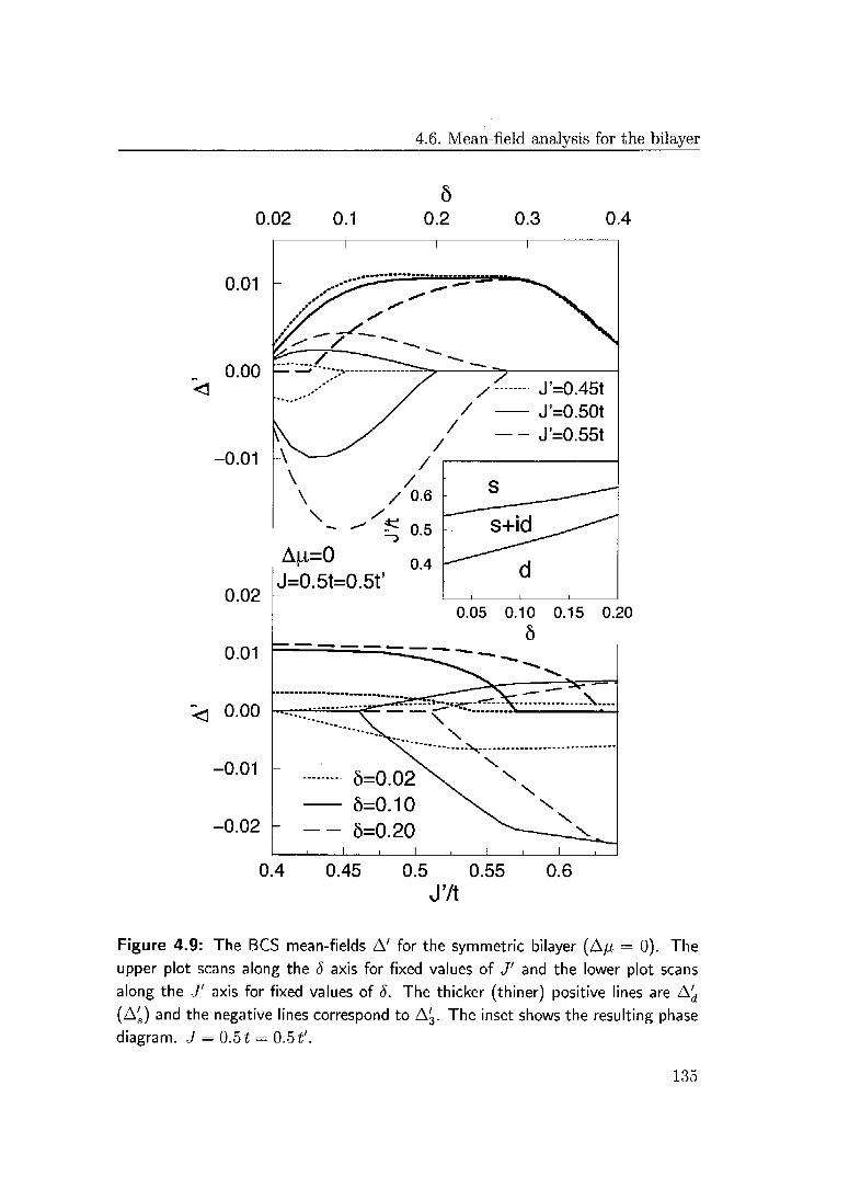
4.6. Mean-field analysis for the bilayer
0.02
0.01 -
0.1
Ö
0.2 0.3 0.4
-0.01
0.02
0.01
< o.oo
-0.01
Afi=0 04
J=0.5t=0.5f
0.05 0.10 0.15 0.20
Ô
0=0.02
0=0.10
-0.02 h -- 6=0.20
0.4 0.45 0.5 0.55 0.6
J'/t
Figure 4.9: The BCS mean-fields A' for the symmetric bilayer (Ap = 0). The
upper plot scans along the 8 axis for fixed values of 3' and the lower plot scans
along the 3' axis for fixed values of 8. The thicker (thiner) positive lines are A^(A^) and the negative lines correspond to A3. The inset shows the resulting phase
diagram. 3 = 0.51 = 0.5*'.
135

4. Inhomogeneously Doped t-3 Ladder and Bilayer Systems
than a splitting, we observe an overall decrease of the correlations with s-wave
symmetry. At a critical value of the chemical potential difference, ApCjS, the
s-wave component disappears in a second order phase transition, leading to a
state with pure <i-wave symmetry. In this state there are still finite pairing
correlations on the upper layer, which are also enhanced due to the proximity
of the lower layer. Increasing Ap further we cross another critical value of Ap,
where the pairing correlations on the upper layer vanish completely and only
the lower layer stays in a superconducting state. This phase we denote by d'.
Note, however, that the transition from d to d' is not a real second order phase
transition, as there is no symmetry breaking associated to it. Therefore we
indicate this transition by a dashed line in the phase diagram.
For 3' = 0.45*, The s-wave component is already marginally small at
Ap = 0 (for 8 = 0.08) and is suppressed almost immediately by increasing
Ap. Comparing the curves of the A'ad in the two figures, we observe that the
presence of a finite s-component reduces the magnitude of the d-component,
but in the d'-phase the curves are identical. Furthermore the value of Aid in
the <f-phase is considerably larger than the value of A^ at 8 ~ 0.16, 3' = 0.45*
in Fig. 4.9. This is due to the fact that in our mean-field calculation, the
d'-phase consists of a Heisenberg layer and a doped t-3 layer, which are com¬
pletely decoupled. In the symmetric case, however, we have two doped layers
which are coupled by the non vanishing mean-field xs which reduces the pairing
correlations.
For larger values of inter-layer exchange coupling, 3' « 0.55* and for small
doping, 8 ~ 0.04, we find a superconducting phase with pure s-wave symmetry
at Ap = 0, as can be seen from Fig. 4.9. Applying different chemical potentials
to the layers increases the hole carrier concentration in the lower layer and
leads to a second order phase transition at Apcd, where the d-wave component
appears and coexists with the s-wave component. For small doping concentra¬
tions and large values of 3' the s-wave component decreases monotonically with
increasing Ap but fails to vanish even at very high values of Ap, the situation
is similar to the situation illustrated in Fig. 4.5, where a crossover from a phase
with strong superconductivity to a phase with weak superconductivity can be
observed at low doping concentrations.
136
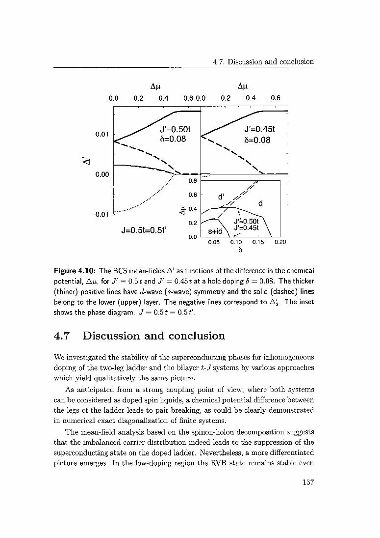
4.7. Discussion and conclusion
A[x À[x
0.0 0.2 0.4 0.6 0.0 0.2 0.4 0.6
T 1 —''
i" t r
Figure 4.10: The BCS mean-fields A' as functions of the difference in the chemical
potential, Ap, for 3' — 0.51 and 3' = 0.45 * at a hole doping S — 0.08. The thicker
(thiner) positive lines have d-wave (s-wave) symmetry and the solid (dashed) lines
belong to the lower (upper) layer. The negative lines correspond to A3. The inset
shows the phase diagram. 3 — 0.5* — 0.5*'.
4.7 Discussion and conclusion
We investigated the stability of the superconducting phases for inhomogeneous
doping of the two-leg ladder and the bilayer t-3 systems by various approaches
which yield qualitatively the same picture.
As anticipated from a strong coupling point of view, where both systems
can be considered as doped spin liquids, a chemical potential difference between
the legs of the ladder leads to pair-breaking, as could be clearly demonstrated
in numerical exact diagonalization of finite systems.
The mean-field analysis based on the spinon-holon decomposition suggests
that the imbalanced carrier distribution indeed leads to the suppression of the
superconducting state on the doped ladder. Nevertheless, a more differentiated
picture emerges. In the low-doping region the RVB state remains stable even
137
4. Inhomogeneously Doped t-3 Ladder and Bilayer Systems
for large differences in the chemical potential and supports a weakly supercon¬
ducting phase. This RVB phase and the weak superconducting state do not
exist for higher doping concentrations above 8 « 0.15.
The conclusions that can be drawn from the mean-field results for the bi¬
layer arc similar to the conclusions for the two-leg ladder, as far as the s-wave
superconducting phase is concerned. A new aspect in 2D is the presence of
another pairing state with d-wave symmetry. This state having no interlayer
pairing amplitudes is only weakly affected by the charge imbalance. Starting
from a strong interlayer s-wave pairing it is therefore possible to induce a tran¬
sition to a c?-wave pairing state by an inhomogeneous doping of the layers. Our
mean-field calculations predict, that this transition occurs as two second order
phase transitions with an intermediate time reversal symmetry breaking phase,
where both the s-wave and the d-wave order parameters are finite.
A modified picture is observed in the renormalization group treatment of
the weakly interacting Hubbard model on the two-leg ladder. Also here in-
homogeneous doping leads to a suppression of the superconducting phase, a
Luther-Emery-liquid characterized by one gapless charge mode (C1S0). More¬
over, an intermediate phase appears which corresponds to a single channel being
superconducting while a coexisting channel forms a Luttinger liquid (C2S1).In both the t-3 and the Hubbard model a phase of complete destruction of
superconducting fluctuations appears for large enough differences in the chemi¬
cal potential. Within the renormalization group approach this normal phase is
characterized as a single Luttinger liquid state (C1S1). While this identifies the
true low-energy properties of this regime, the change in the spinon spectrum
discussed in Sec. 4.5 rather reflects a short-coming of the mean-field solution.
In conclusion we emphasize that inhomogeneous doping is harmful for the
formation of the superconducting state in the two-leg ladder and for the s-wave
superconducting state on the bilayer. Furthermore, inhomogeneous doping of
the legs of the ladder or of the layers can be an interesting tool to access new
phases for this type of systems.
138

Chapter 5
Existence of Long Range
Magnetic Order in the Ground
State of Two-Dimensional
Spin-1/2 Heisenberg
Antiferromagnets
5.1 Introduction
The first mathematical proof on the existence of long range order (LRO) at low
temperature and therefore the existence of a finite temperature phase transition
for classical systems with a continuous symmetry group was given by Fröhlich
et al. in Ref. [146, 147] The central part of their proof lies in the derivation
of an upper bound for the continuous part of the two-point function. Soon
afterwards, Dyson, Lieb, and Simon (DLS) [148] extended the proof to quantum
spin systems, including the antiferromagnetic Heisenberg model with spin larger
than 1/2 and dimension larger than 2.
For two-dimensional quantum spin systems with complete spin rotation
symmetry there is no LRO at finite temperature based on the Mermin-Wagner-
Hohenberg theorem. However, the question whether the ground state has LRO
or whether it is disordered by quantum fluctuations is a question which has not
been resolved rigorously for all cases.
Nevez and Perez [149, 150] extended the method of DLS to zero-temperature
139

5. Antiferromagnetic LRO in 2D Spin-1/2 Heisenberg Systems
and proved the existence of LRO for the two-dimensional antiferromagnetic
Heisenberg model in the ground state for spin larger than 1/2. Improving the
method of DLS further, Kennedy, Lieb, and Shastry (KLS) [151] succeeded
in proving the existence of LRO in the ground state of the three-dimensional
antiferromagnetic Heisenberg model with spin-1/2. Further, they approached
the two-dimensional spin-1/2 case by decreasing the antiferromagnetic cou¬
pling in the third dimension. Kubo et al. [152] and Ozeki et al. [153] studied
the spin-1/2 antiferromagnetic XXZ model on the square lattice and showed,
that for a large enough as well as for a small enough anisotropy parameter,
A — 3Z/3X, LRO in the ground state exists. Until now, however, there is no
mathematical proof for the existence of LRO in the ground state of the two-
dimensional SU(2) symmetric antiferromagnetic Heisenberg model for spin-1/2on the square lattice. Parreira et al. [154] demonstrated that for an antifer-
romagnet that consists of 8 layers, that are coupled antiferromagnetically and
with periodic boundary conditions along the third dimension, LRO exists.
A very interesting and physically very relevant system is the spin-1/2 an¬
tiferromagnetic Heisenberg bilayer. A small antiferromagnetic inter-layer cou¬
pling tends to stabilize the antiferromagnetic LRO and to reduce the effect of
the quantum fluctuations. On the other hand the inter-layer coupling must not
be too strong, as in this case local singlets are formed which destroy the anti¬
ferromagnetic order and lead to a quantum disordered ground state [144, 145].
Although the rigorous proof of the existence of antiferromagnetic LRO should
be easier for the bilayer than for the single layer, it still remains an open prob¬
lem.
In this chapter, extending the methods introduced by Kennedy et al. [151],we will show that already for 4 weakly coupled layers LRO exists in the ground
state. Further, we will study two different Heisenberg models on the bilayer
lattice. The first one contains in addition to the nearest-neighbor antiferro¬
magnetic couplings also ferromagnetic next-nearest-neighbor (nnn) inter-plane
couplings. If these additional couplings are strong enough, we can prove the
existence of LRO in the ground state. Finally we will study two antiferromag¬
netic spin-1/2 layers that are coupled by antiferromagnetic nnn couplings. If
the inter-layer and the intra-layer couplings are of about the same strength,
the existence of LRO in the ground state can be proven.
140

5.2. N layers with nearest-neighbor couplings
5.2 TV layers with nearest-neighbor couplings
We study an antiferromagnetic Heisenberg model with nearest-neighbor inter¬
actions on the following hypercubic lattice
A - {a e Z3|l < «i < L, 1 < a2 < L, 1 < a3 < N}, (5.1)
where L and N are even numbers, and |A| — NL2. The Hamiltonian is given
by
H = Y, (Sa • Sa+51 + Sa • Sa+Is2 + T Sa • Sa+äJ . (5.2)aeA
The coupling along the third direction can be tuned by the parameter r and
periodic boundary conditions are implied in all directions. For every q =
2ir(ni/L, n2/L, n3/N) we define the Fourier transformed spin operators
5 = -_Ly e-iqa5^, S± = -^= Ye"iqa (Sx ± iSl), (5.3)
and write the Hamiltonian as
H=YE* \S-«S« + \ (54^q + S-X) (5.4)
with Eq — cosçi + cosç2 + rcosg3. The ground state of H is non-degenerate
[155] and we denote with (•) the expectation value of an operator in this ground
state. For the two-point function
$q = (S^Sq) > 0 (5.5)
the following sum rules hold,
1^ S(S + 1) 1
TÄf5Z^ 3 4'(5"6a)
q
where —e is the ground state energy per lattice site. The usual strategy to prove
the existence of long-range order in the ground state is to find an upper bound
for <7q for almost all values of q and then to show that in the thermodynamic
limit a finite contribution to the integrals of the sum rules (5.6) must come
from the single q points, where the bound of gq is divergent.
141

5. Antiferromagnetic LRO in 2D Spin-1/2 Heisenberg Systems
The two-point function, gq, can be expressed as an integral over the spectral
weight function R(u) = \ En(IH5ql°)l2 + IH#-q|0)|2) 8(u-En + EQ), where
\n) are eigenstates of H with energy En and 0 denotes the ground state. From
the Cauchy-Schwarz inequality we obtain
 =
2
duR(u) <(! duR(u)uj J ( / duR^uj-1 J . (5.7)
i([[Sq,#],S_q]> Xq
where Xq is the magnetic susceptibility. Using the commutation relations
1 1
[-Sq i -Sq'] = ±/T-rj S'q+q' [<Sq , <5q'] = /r-g
2^q+q' (5-8)
we can calculate the double commutator
[[Sq, H], S„q] = i^| E v57«' +^ - 2^') ^ (5î5:q' + 5Ä) • (5"9)
We introduce now the quantities
pi = -(Sa-Sa+(5() = -j— ^#q cos?; / = 1,3, (5.10)' '
q
for which the relation
e = 2p1 + rpz (5.11)
holds. For the expectation value of the double commutator (5.9) one obtains
1 2
-([[Sq,H],S-q]) = -[e- pi(cosq1 + cos q2) -rp3cosq3}. (5.12)
Using the reflection positivity of the system, KLS a showed that the suscepti¬
bility is bounded by
*>s4(2+r+g,)-
(513)
With (5.7), (5.12), and (5.13) we obtain the upper bound
*-*=vll JTTT^ ) (514)
"Note, that E^ in the notation of KLS corresponds to 2 + r — i?q in our notation.
142

5.2. N layers with nearest-neighbor couplings
The exact values of the pi are not known. It is possible to derive an upper
bound that is bigger than (5.14) but only depends on the energy e [151, 154],
It turns out, however, that the integrals depend quite strongly on the upper
bound and therefore we will work directly with the upper bound of Eq. (5.14),
which is the best possible bound within this method. Therefore, in order to
prove the existence of LRO in the ground state, we must show that for the whole
range of possible values of e, pi, and p3 the continuous part of the two-point
function gq cannot be sufficient to fulfill the sum rules (5.6).The following (Anderson) bound for px holds (Theorem C.2 of DLS [148]):
Pi < PT - ^p (5-15)
where n\ is the number of equivalent neighbors. In our case n\ = A and n$
equals 1 for the bilayer and 2 for 4 or more layers in the 3-direction. The
absolute value of the energy per site, e, is bounded by
eN < e < Ca (5.16)
where eN — (2 + r)/A is the Néel bound and ex is the Anderson bound for the
ground state energy given by (App. C.l)
§ (l + 2r + V25 - 8r + 16r2) UN = 2,
CA = { ; / (5.17)M 1 + r + V25 + 2r + 9r2) iî N > 2.
With Eq. (5.11), (5.15), and (5.16) we have therefore restricted the possible
values of e, pi, and p3 to a finite, two-dimensional parameter space A. To show
the existence of LRO in the ground state, we first define the functions
a(a) = Um -^ft, 6(a -Eq)-± (5.18a)J_>°° ' '
q#Q
b(a) = limi^ g^Eqe(a-Eq) + e-, (5.18b)
where Q — (n, it, tv) is the antiferromagnetic ordering vector. The system has
LRO in the ground state, if for all (pi,p3) A either a(oo) < 0, which states
the impossibility to fulfill sum rule (5.6a) with the continuous part of gq, or
&(0) > 0, which states the impossibility to fulfill sum rule (5.6b). If there
143
5. Antiferromagnetic LRO in 2D Spin-1/2 Heisenberg Systems
are however points in A, where both sum rules can be fulfilled separately, we
can still check, for the case where 6(0) < 0 < b(oo), whether it is possible to
fulfill both sum rules simultaneously. If there is an a0 > 0 with b(a0) — 0 and
0,(0/0) < 0, it is not possible to fulfill both sum rules simultaneously, because
of all functions gq with 0 < gq < gq that satisfy (5.6b), the function gq =
gq0(ao — Eq) maximizes the r.h.s. of (5.6a). For further details we refer to KLS
[151]. In summary, we can prove the existence of LRO if the condition
0(00) < 0 V b(0) > 0 V (b(a0) = 0 A a(a0) < 0) V(pi, p3) e A (5.19)
is fulfilled. For a given value of r and of N we scanned the entire parameter
space A, and we can prove with this method the existence of long-range order
for the three-dimensional case if r > 0.14. If we reduce the number of layers
in order to approach the 2-dimensional case, we can rigorously show that for 4
layers with r > 0.16 we have long-range order. If r is large the 4-layer system
consists of weakly coupled square plaquets which in the limit of infinite r form
a plaquct singlet state without LRO in the ground state. However, we can show
that for 4 (or more) layers and 0.16 < r < 2.1 LRO in the ground state exists.
For the bilayer system, we were not able to prove the existence of magnetic
order for any value of r. This rather abrupt change from 4 to 2 layers is due
to the fact that the number of neighboring spins is reduced from 6 to 5 in the
bilayer. Attempts to split the sum rule (5.6b) into two separate sum rules for pi
and p3 and to request that all three sum rules should be satisfied simultaneously
were still insufficient to prove LRO for the bilayer system. This is somewhat
unfortunate, because the bilayer would be a physically more relevant system
than the four layer system with periodic boundary conditions. In the next
section, however, we show the existence of LRO for a modified bilayer system.
5.3 Antiferromagnetic bilayer with ferro¬
magnetic next-nearest-neighbor coupling
The simplest way to reduce the effects of the quantum fluctuations and to sta¬
bilize the antiferromagnetic ground state is to introduce ncxt-nearest-neighbor
(nnn) ferromagnetic couplings. It is not possible to apply the methods of reflec¬
tion positivity to quantum mechanical Heisenberg models with ferromagnetic
nearest-neighbor exchange couplings. For example, there is still no rigorous
proof, that the ferromagnetic spin-1/2 Heisenberg model on the cubic lattice
144

5.3. Bilayer with ferromagnetic next-nearest-neighbor coupling
Figure 5.1: (a) The bilayer lattice with antiferromagnetic nearest-neighbor cou¬
plings (blue) and ferromagnetic nnn inter-plane couplings (red), (b) The bilayer
lattice with antiferromagnetic inplane nearest-neighbor couplings and antiferromag¬
netic nnn inter-plane couplings.
has a finite temperature phase transition. However, in this section we will show
that the method of reflection positivity can be applied on hypercubic lattices
with ferromagnetic nnn Heisenberg couplings, if strong enough antiferromag¬
netic nearest-neighbor couplings are present. It is for example possible to apply
the method of reflection positivity to the famous 3\-32 model on the square lat¬
tice with 0 < — 32 < Ji/2. However, it turns out, that also the addition of the
diagonal ferromagnetic couplings does not allow to prove LRO in the ground
state.
In the following we study a spin-1/2 antiferromagnetic Heisenberg model
on the bilayer with ferromagnetic next-nearest-neighbor inter-layer couplings
as shown in Fig. 5.1 (a) with the Hamiltonian
a£A
\ 2
- Sa ' Sa+Ja + ^ Sa (S^^. — T Sa+^+öa)j-1
(5.20)
Note that the sum over a runs over all lattice sites. We use periodic boundary
conditions and therefore the coupling along <S3 is also 1. Further, we assume
0 < r < 1/4 for the ferromagnetic coupling between the layers. With the
definition (5.3) we can write H in the form (5.4) with Eq given by
Eq = (1 - r cos <?3)(cos qi + cos q2) + - cos q3. (5.21)
145

5. Antiferromagnetic LRO in 2D Spin-1/2 Heisenberg Systems
For the expectation value of the double commutator (5.9) one obtains
1 n 22
Dq:=-([[Sq,H],S.q}) = f(l-cosç3) + 3£>(l-cosgi) (5.22)
22
+Ö S rpd(1 ~ C0S q3 C0S 93)'6
j=l
with p; defined as in (5.10) and with
=
|A|
Q
Pu = (Sa • Sa+Sj+Ss) = TTT Y 9* COS *' C0S qZ' (523^q
Further, we have the relation
e = -(4p1+p3 + 4rpd), (5.24)
and —e is the ground state energy per lattice site.
We derive now an upper bound for the susceptibility. The first step is to
apply the unitary transformation, that rotates all the spins on a sublattice by
7T around the y axes, i.e., we obtain new spin operators Ta that are related to
the original spin operators Sa by
T* = eiCl*Sx, Ty = Sy, Tl = eiQa Sza, (5.25)
where Q = (it, it, it) as before.
We want to use the reflection symmetries of the lattice in order to derive
an upper bound for the susceptibility. For every pair of parallel planes that
separate the lattice A into two equal subsystems the Hilbert space is the direct
product of the two Hilbert spaces associated with the two subsystem, H =
Hi®H\. The reflection at the two planes allows to associate to each operator
A ® 1 := A an operator 1 ® A := À. The Lemma 6.1 of DLS [148], in the
zero-temperature limit, states that the ground state energy of the Hamiltonian
H(hi) = A + B + Y(d ~ âi ~ ^? ~ Y&i ~ Vrf (5-26)i j
is bigger than the averaged ground state energy of the Hamiltonians
HA = A + Ä + Y(Ci-Ci)2-Y,(VJ-Vrf (5-27a)i j
HB = B + B + Yid-CiY-Y&i-VjY, (5-27b)
146
5.3. Bilayer with ferromagnetic next-nearest-neighbor coupling
i.e.,
E[H(hi)} > (E[HA] + E[HB})/2, (5.28)
where E[H] denotes the ground state energy of the Hamiltonian H. In (5.26)and (5.27) A, B are self-adjoint operators, d are real self-adjoint operators
and T>j arc imaginary self-adjoint operators. Further, hi are real numbers. We
decompose the Hamiltonian (5.20) into the three terms H — Hx + Hy + Hz.
The Hamiltonian Hy can up to constant terms be written as
B. = EaeA L
l-4r
(vi-n^y Ë (Ta ~ Ta+,,i=i
—
L V^ (tv— Ty —Ty 4-Ty ~\
4 Z_^ \ a a+öj ^a+Sa~
Ja+Sj+S3 J
3=1
(5.29)
which is of the form (5.26) for all symmetry planes of the bilayer that contain
no lattice sites. Note, that in our notation Ty are imaginary operators. The
terms Hx and Hz, containing the real operators Tx and T*, can not be written
in the form required by (5.26) for all symmetry planes of the bilayer. However,
we can define the Hamiltonians
KiK) = YaeA
+1 - Aur f
A \
2
[Ta
2
2
rpz
1a+S3
rpz1a+öi
8u,+K,
8„_h*AJv,- (5.30)
j=i
with v — ±1, 8 is the Kronecker symbol, and
ha.,1
v
aj
ha+öt'— 1) 2,3,
Ci — ^a + ^^a+<5,- — Vha+s3 — /la+o.+fo,
(5.31a)
(5.31b)
where ha is a real valued function on the lattice. Note that that H* is of the
form (5.26) for the symmetry planes perpendicular to <53, whereas H~ is of the
form (5.26) for all symmetry planes parallel to <53. In an analogous way we
define Hvx by replacing z with x and and setting ha — 0 in (5.30) and finally,
we define
HV(K) = HI + Hy + H:(ha) v = ±. (5.32)
147

5. Antiferromagnetic LRO in 2D Spin-1/2 Heisenberg Systems
For ha — 0 both Hamiltonians #^(0) are up to constant terms equal to the
original Hamiltonian H. From (5.28) it follows that (App. C.2)
E[HV(K)\ > E[Hu(0)] for v = ±. (5.33)
The next step is to calculate E\Hv{hg)\ in second order perturbation theory in
ha. The linear terms in i7t/(/ia) are given by
-K2
V{hJ = ^f(^-«-3 " hj) + Su,- Y fa-;* - h°>i)aeA
Lj=l
2
-2r8v- (ha+63 + ha„Ö3) - r8v!+ Y [h^+s3 + ha+ö,J (5.34)
2
+ Y, o (^a+*j+** + K+ôj-03 + hz-Sj+Sz + Ksj-SiJ3=1
Choosing ha as
ca = cos(q • a)/v/jÄ[ sa = sin(q a)/v^Ä[ (5-35)
we obtain with (5.3)
^(ca) = -(Tq + T_q)/£, V(aa) - -z(Tq - T_q)/q^, (5.36)
with Tq — S'q+Q and
fq — (1 — cosg3)(l/2-I-rcosçi+rcosç2)> (5.37a)
/" = (2 - cosçi -cosç2)(l +rcosç3). (5.37b)
The quadratic terms in the Hamiltonian (5.30) are given by
qv(K) = 1~^8V>+ hl> + Y (V"^'-^ +4 (<^)2) ' (5-38)
3=1
and for the fields ca and sa we find the relation
g"(Ca) + 9,'(Sa) = /q for i/= ±. (5.39)
Applying second order perturbation theory in sa and ca and summing up all
second order terms, we obtain from (5.33) the inequality
0<£ +4W4£!Ä!5MM (5,0)
"Xq+Q
148
5.3. Bilayer with ferromagnetic next-nearest-neighbor coupling
which yields the following upper bound for the susceptibility
Xq < Xq = minj7ï— (5-41)
"
4->q+Q
With (5.7), (5.22) and (5.41) we obtain an upper bound for gq
Sq < £q = V^qXq- (5-42)
In order to use this upper bound we need bounds for the expectation values pi,
P3, pd and for the energy e. We find the following bounds:
(5 + 4r)/8 < e < (7 + 4r)/8 (5.43a)
1/8 < pi < 3/8 (5.43b)
0 < Pa < 3/4 (5.43c)
0 < pd < 1/4 (5.43d)
Note, that all the ground state expectation values of pi, p3, and pd (cf. (5.10)and (5.23)) must be positive, because all off-diagonal matrix elements in the
eigenbasis of the Ta operators are negative. From (S* Sj) < 1/4 follows the
r.h.s. of (5.43d). From -(Si • S,-) < 3/4 follows the r.h.s. of (5.43c). From
(5.15) with ni = A follows the r.h.s. of (5.43b) and the r.h.s. of (5.43a) follows
from (5.24), from the Anderson bound (5.15) with n\ — 5 and from the r.h.s. of
(5.43d). The l.h.s. of (5.43a) comes from the Néel state. The l.h.s. of (5.43b)follows from (5.24), the l.h.s. of (5.43a), and the r.h.s. of (5.43c) and (5.43d).
Now, we can again define the functions (5.18) and use the condition (5.19)to prove LRO. In fact for 0.21 < r < 0.25 we can prove LRO by scanning
the whole three-dimensional parameter space A 3 (pi,p3,pd) defined by the
equations (5.43). Note, that our method requires r < 0.25. It is however easy
to prove the existence of LRO for r — oo,b where the systems consists of two
antiferromagnetically coupled classical spins. This gives us good reasons to
believe, that the systems will have LRO in the ground state for all values of
r > 0.21.
bDenoting by SA (S#) the ^-component of the total spin operator on sublatticc A (B), we
have (gQ) = (^(S'A - S|)2> = (2((SA)2) + 2((£|)2) - <S&t))/|A|. As in the ground state
SU = 0, and for large r we have limr^0O((5i)2) = limr^00(Si)/3 = (|A|/4)[(|A|/4) + l]/3and the same for ((5b)2), we find therefore \imr^co(gQ) = |A|/12 + 0(1).
149
5. Antiferromagnetic LRO in 2D Spin-1/2 Heisenberg Systems
5.4 Diagonal bilayer
In Sec. 5.2 we saw, that it is difficult to prove LRO on the bilayer for antiferro¬
magnetic rung coupling. On the other hand we know, that for infinitely strong
ferromagnetic rung coupling, the bilayer reduces to a square lattice of spin-1
moments, for which the existence of LRO in the ground state has been rigor¬
ously established [151]. Therefore, an alternative way to approach the spin-1/2
square lattice would be to reduce the ferromagnetic rung couplings to finite
values. But it is not possible to apply the ideas of reflection positivity to quan¬
tum Heisenberg models with ferromagnetic nearest-neighbor couplings.0 It is
possible to mimic the ferromagnetic rung coupling by nnn antiferromagnetic
couplings and Kishi and Kubo found a way to prove LRO in frustrated systems
with antiferromagnetic nearest- and next-nearest-neighbor couplings [156].
Motivated by these ideas we consider in this section the spin-1/2 bilayer
with the following antiferromagnetic Hamiltonian
2
H = D JL (Sa •s*^+r Sa • s*+*i+**) (5-44)aeA j=l
The two layers are connected in a diagonal way by antiferromagnetic couplings
as shown in Fig. 5.1 (b) but they are not connected by perpendicular couplings.
For r = 1 this Hamiltonian depends only on the operators Sa,+ — Sa + Sa+s3
Therefore the operators Sa + commute with the Hamiltonian H and therefore
the eigenstates of H can be chosen to be eigenstates of Sa +,too. Alternatively,
one can consider the unitary transformations <Sa, that exchange the sites on the
rung a. For r — 1 these are symmetries of the Hamiltonian and the parity of
this local reflection is related to the eigenvalues of S^+.It is easy to see that in the ground state the eigenvalue of each Sa + must be
2, i.e., the two spins must form a spin-1 moment.d We can reduce therefore the
cIn order to apply the methods of reflection positivity, we should write the Hamiltonian in
the form (5.26). For the antiferromagnct we can apply local unitary transformations which
change the sign of Sx and Sz. There is however no unitary transformation on C2, which
only changes the sign of Sy, and such a transformation would be needed in the ferromagnetic
case.
dLet us assume that the ground state is in the sector with 52+=0. In this case we
can write the wave function in the form \ipo) = |sa) ® |V>')i where sa stands for a singlet at
site a. However, the wave function |V>i) = \t1) ® \ip') has the same expectation value of the
Hamiltonian and lies in a different sector of the Hilbert space. We know that the ground
state is not degenerate [155] and therefore \ipo) can not be the ground state.
150
5.4. Diagonal bilayer
Hilbert space to the subspace where S^+ = 2 for all a. Within this subspace,
the problem is equivalent to a S — 1 Heisenberg model on the square lattice,
which is known to have long range order [151].For r — 1 the Hamiltonian H is effectively a spin-1 and not a spin-1/2
Hamiltonian, but we will now show that also for r < 1 LRO exists, and that
the existence of LRO is not restricted to the case where effective spin-1 moments
are present. For r — 0 our model describes two independent spin-1/2 square
lattices. In this sense, we can interpolate with our model between the spin-1
and the spin-1/2 case.
The strategy of the proof is again to derive an upper bound for gq for
almost all values of q using the inequality (5.7). The double commutator is
straightforward to calculate and is given by
1 2
-([[Sq, H], 5_q]> = - [e - (pi + rpd cos g3) (cos 9l + cosq2)\, (5.45)
where pd = — (Sa • Sa+<51+(s3) and e = 2(pi + rpd). To find an upper bound
for the susceptibility we rotate all the spins on one sublattice by it around the
?/-axis. With this unitary transformation the local spin operators (Sx,Sy,Sa)transform to the new spin operators (Tx,iTy,Ta), given by
Tx = eiQaSx iT% = Sl T* = eiQaSza, (5.46)
where Q = (ft^, 0). We define the Hamiltonian
2
H(h*) = ^EË (l-r)(T.-T^-hilj)a + r(Ta-Ta+,,)2a j—1
L
+ T~ (Ta + Ta+Ô3 - Ta+Ôj - Ta+53+Sj - hg)2
(5.47)
with b4j = (0,0, haj). This Hamiltonian is of the form (5.26) for all pairs of
symmetry planes parallel to 63. Using (5.28) and the same arguments as in
Appendix C.2, wc can show that
E[H(ha)} > E[H(0)}, (5.48)
where ^[^(^a)] denotes the ground state energy of the Hamiltonian H(ha).Note that the Hamiltonian H(0), i.e., the Hamiltonian (5.47) with all hjj — 0,
is up to a constant term equal to the Hamiltonian H in (5.44).
151

5. Antiferromagnetic LRO in 2D Spin-1/2 Heisenberg Systems
We now calculate the terms in E[H(ha)] that are quadratic in the fields for
the following specific choice of the fields
^a,j ~ ha — ha+0j haj = ha + ha+s3 — ha+6j — ha+s3+5j
The linear terms in H(ha) are given by
v(ha) = YT>aj
(ha+Sj + h^ö - 2ha) - r(ha+s3 + K_s.d) (5.49)
r
+ -^(ha+03+ôj + K+äz-äj + ha_ös+sJ + ha^03~Sj)
and choosing ca and sa as in (5.35) we obtain V(ca) = — (Tq + T_q)/q and
V(sa) = -i(Tq - T_q)/q with Tq = Sq+Q and with
2
/q = ^(1 -cosqj)(l+rcosq3). (5.50)i=i
The quadratic part of H(ha) is given by
<7(/?'a) =« Y^1 "~ r) (h* ~ h*+6j) +
9ih* + ha+ö3 ~ K+ôj ~ ta+Äa+Jj)'
aj
(5.51)and we have the relation q(sa)+q(ca) = /q. Applying second order perturbation
theory in sa and ca and summing up all second order terms, we find again the
inequality (5.40) (without the v index) which is equivalent to Xq < l/(4/q+oJ-
Finally, we obtain with Eq. (5.7) and Eq. (5.45) the upper bound
9q < Ve ij = sß p + 2Ar-(l + Arcos,3)(ccS,1+coS,2)\ 1
V 12(l + Ar)/q+Q J
with pd — Xpi. Note, that this upper bound diverges at the two q values
Q = (tt, tt, 0) and Q' ~ (tt, tt, tt). The divergence of the magnetic susceptibility
at the point Q is expected for our system. That the bound for the magnetic
susceptibility is also divergent at Q' is due to the fact, that in the derivation of
Eq. (5.52) only reflection planes parallel to <53 but not the plane perpendicular
to 53 could be used.
From the sum rule (5.6b) we can deduce, that the diagonal bilayer has LRO
in the ground state, if for all possible values of A we have
Us.®£,*-** <¥-W' (5'53)
152

5.5. Discussion and conclusion
with Eq — (cos Çi + cos q2)(l + r cos q3). It is clear that for r < 1 we must have
0 < A < 1.° But in addition we have the inequality en < 2(1 + Ar)pax which
gives us with p** from (5.15) the following range of possible values of A
max(0, (2r - 1)1Zr) < A < 1. (5.54)
The numerical evaluation of the integral (5.53) for the whole range of possible
values of A shows that we have LRO for r > 0.85. Note, that for r = 1 we have
A — 1 and a flat band with Eq — 0. In this case the condition (5.53) for LRO
reduces to the condition for a spin-1 system on the square lattice.
5.5 Discussion and conclusion
We extended the method of DLS and KLS for proving the existence of an¬
tiferromagnetic LRO, by scanning not only the whole possible energy range
(e), like in the work of KLS, but also scanning all possible ratios between the
Heisenberg terms (pi) on non-equivalent bonds. In this way we could show an¬
tiferromagnetic LRO for various two-dimensional spin-1/2 Heisenberg models.
We approached the two-dimensional Heisenberg model on the square lattice
in two different ways:
First, we started from the three-dimensional spin-1/2 antiferromagnet and
then reduced both the number of layers in the third dimension and the coupling
along this direction. For 4 layers, only a weak inter-layer coupling (r = 0.16)
is required for proving LRO, but for the bilayer, where the number of nearest-
neighbors is reduced to 5, the current method fails to show the existence of
LRO.
Further, we could show that the antiferromagnetic bilayer with small fer¬
romagnetic diagonal couplings (r > 0.21) between the layers has LRO in the
ground state. One can view this as approaching the quantum mechanical two-
dimensional case from the classical zero-dimensional case, as for very large fer¬
romagnetic couplings the system reduces to two antiferromagnetically coupled
classical spins.
Finally, we approached the single layer spin-1/2 antiferromagnetic Heisen¬
berg model on the square lattice by starting from an effective spin-1 antiferro-
eThis follows from the operation S = F[ed a=1 <Sa that exchanges the two sites for every
rung with eQ a= 1. With this operation the bonds with coupling r are mapped on bonds
with coupling 1 and vice versa. For r < 1, we must have A < 1 in the ground state, because
otherwise we could apply <S to the ground state and obtain a state with lower energy.
153
5. Antiferromagnetic LRO in 2D Spin-1/2 Heisenberg Systems
magnetic Heisenberg model on the square lattice, that consists of two diagonally
coupled layers. Here, the inter-layer coupling strength r G [0,1] interpolates
continuously between spin-1/2 and spin-1 square lattice Heisenberg models.
We showed that for r > 0.85 there exists LRO in the ground state.
We believe that there is space for improvement of the present ranges of
validity by further extensions of the method of "Gaussian domination". Indeed
our analysis shows that the bilayer system does only marginally not satisfy the
conditions within the present scheme. Moreover the range of validity of the
proven long range order in the diagonal bilayer system could be considerably
extended, if the mock divergence at (tt, tt, tt) of the upper bound for the sus¬
ceptibility could be eliminated. The rigorous proof of long range order in the
two-dimensional spin-1/2 Heisenberg model on a square lattice with nearest-
neighbor coupling remains, however, still a formidable task and essentially new
techniques might be required.
154

A
Appendix to Chapter 2
A.l Definitions of the pocket operators
The equivalence of the two definitions for the pocket-operators made in Eq. (2.9)and in Eq. (2.8) follows from
1h\j
— _X^J*j-ai02
I
t'Kma
I Y^ ciB'-a' Y^ eiK-(R+ai+am)a2^ y/N ^
Rma
_ -iBjam1 V^ i(K+Bj-)-(R+ai+am) J
v^lR
= e-te^i+Bi)Bff. (A.l)
The diagonal form of the tight-binding Hamiltonian in Eq. (2.11) follows di¬
rectly from the relation
e"""'
— 0-iBi-(am-am/) mm'
K+B= e-iBr(a«-am')eTOm _ (A.2)
A.2 Derivation of the effective Hamiltonian
Here, we provide some details concerning the derivation of the effective Hamil¬
tonian in Eq. (2.19). It is convenient to treat each term in Eq. (2.15) separately.
155
A. Appendix to Chapter 2
Let us start with the Hund's coupling.
17 / j / jCrmaCTm'a'Crma'Crm'a {^-^J
r m^m'
~
2ÏV ^ -^ Ckm(rCk'mV'V^'Cq'mV (A~V
kqk'q' m^m'
=JïL Y y^r Y^ ei(Bi"Bfc)'amci(Bi~Bj)a"1' • (A.5)
kk'q ijkl mj=m'
.
hi* tfl hk hPwKm<7 -k+q m'a' -k'+q ma'VmV'
The sum over the momenta in (A.4) is restricted such that k + k' — q — q'
equals a reciprocal lattice vector. (A.5) follows from (A.4) by using the defini¬
tion of the pocket operators in Eq. (2.8). The sum over the pocket indices is
again restricted such that Bj + Bj + b^ 4- B; equals a reciprocal lattice vector,
whereas the sum over the momenta in the reduced BZ is simplified to an unre¬
stricted sum over three momenta. Note that this is a good approximation for
small pockets, because all the processes at the Fermi energy are kept. a
The next step is to go from orbital operators to the band operators. Re¬
stricting ourselves to the top band and taking into account Eq. (2.16) we can
simply substitute b]ima —» 4g&K<T- Now we can sum over the orbital indices
in Eq. (A.5) and taking into account that the sum over the pocket indices is
restricted we obtain the sum
Y ei(B*-B*Ham-a/) - 2(A8ik - 1), (A.6)rn^m'
and for the Hund's coupling term
q| E Er&b-W 6-k'+Q.' &„(4*fc " !) (A-7)kk'q ijkl
The restriction of the sum can be dropped, if we replace (A8ik — 1) with (28ijki —
eljki ~ S%i83k — 8%j8ki + Z8ik8ji). The terms proportional to JH in the interaction
of Eq. (2.19) are now obtained by dividing Eq. (A.7) into two equal parts,
rewrite one directly in terms of density-density operators, and rewrite the other
in terms of density-density and spin-density spin-density operators using the
SU(2) relation 28a$8ß1 — 8ai8ßs + aan
' <?ßä- Terms which renormalize the
chemical potential are dropped. All the other terms in Eq. (2.15) are treated
in the same way.
"Small pockets means here 4kf < |bi|, this corresponds to a doping with x > 0.55
156

A.3. The symmetry group G
A.3 The symmetry group G
The symmetry group G of H0a (2.29) is a finite subgroup of U(4) that is gen¬
erated by t the permutation matrices V G S4 and the diagonal orthogonal
matrices V e (Z2)4. G is a semi-direct product of <S4 and the normal sub¬
group (Z2)A. This allows us to find the irreducible representations of G, cf.
Ref. [157]. The elements can be written in a unique way as (V, V) with V G <S4
and V G (Z2y. The product of two elements (V,V) o (V,V) is given by
(V o V',V"). From this follows that if (V,V) is conjugate to (V',V), V is
conjugate to V, and the class of (V,V) G G can be labeled by the class of
V G <S4. The elements of <S4 can be classified by writing them as disjunct cyclic
permutations. We label the five classes as follows: e—1, f—(ab), g=(ab)(cd),
h=(abc), i=(abcd). In total there are twenty 20 classes in G. The character
table is shown in Table A.l. The character corresponding to the natural repre¬
sentation of G by orthogonal 4x4 matrices is xu- The representation on the
16 dimensional space V spanned by Q0-15, that was defined in Sec. 2.4, acts
irreducibly on the subspaces V0, Vl~3, V4"9, and y10-15 with the characters
Xo, X7, X15, and xie, respectively.
With help of Schur's Lemma, it is now easy to show that the interaction
HeS in the Basis Q°~lb is diagonal, i.e.,
YQr3iAW^l = 5rr'K/S> (A.8)ijkl
and that the coupling constant A£ depend only on the irreducible subspace.
As discussed in Sec. 2.5, the subgroup (Z2)4 describes gauge symmetries,
that are broken in the real system whereas the subgroup <S4 describes the space-
group symmetries. The subgroup $4 consists of the classes ei, /1, gi, hi, and i\.
The irreducible representations of G are in general reducible for the subgroup
<S4. For example we have xi ~ ^5, Xi5 — Ti G) T3 © r5, and xi6 — T4 © r5.
157

A. Appendix to Chapter 2
Table A.l: The character table for the symmetry group G of the effective Hamil¬
tonian Heff. The first line labels the classes and gives the number of elements in
each class. The letters of the classes indicate classes of the subgroup <S4: e=l,
f=(ab), g~(ab)(cd), h=(abc), i=(abcd). The characters appearing in our effec¬
tive Hamiltonian are Xi f°r Q°. Xi f°r Q1^3- Xis f°r QA~9 (real matrices) and Xie
for Q10-15 (imaginary matrices). Xn is the natural representation of G defined in
Sec. 2.4. The last column gives the reduction of the representations into irreducible
representations of the subgroup <S4, that consists of the classes ei, fi, gi, hi, and
*i-
ei e2 e3 e4 e5 /i f2 f3 /4 /5 /6 ffi .92 53 ^i h2 h3 h4 it i2 reduction
# 1 4 6 4 1 12 12 24 24 12 12 12 24 12 32 32 32 32 48 48 to <S4
Xl 1 1 1 1 1 1 1 1 1 1 1 1 1 1 1 1 1 1 Tj
X2 1 1 1 1 1 ï I ï i ï ï 1 1 1 1 1 ï ï r2
X3 1 ï 1 ï 1 1 ï ï 1 1 I 1 ï 1 1 ï 1 ï Ti
X4 1 ï 1 ï 1 ï 1 1 î I 1 1 ï 1 1 ï ï 1 r2
X5 2 2 2 2 2 0 0 0 0 0 0 2 2 2 ï ï 0 0 r3
X6 2 2 2 2 2 0 0 0 0 0 0 2 2 2 ï 1 0 0 r3
X7 3 3 3 3 3 1 1 1 1 1 1 ï ï ï 0 0 0 0 ï ï r5
Xs 3 3 3 3 3 ï I ï I 1 1 1 1 1 0 0 0 0 1 1 r4
X9 3 3 3 3 3 1 ï ï 1 1 ï ï 1 ï 0 0 0 0 ï 1 r5
X10 3 3 3 3 3 I 1 1 ï ï 1 ï 1 ï 0 0 0 0 1 ï r4
Xn 4 2 0 2 4 2 2 0 0 2 2 0 0 0 1 ï 1 ï 0 0 rier5
X12 4 2 0 2 4 2 2 0 0 2 2 0 0 0 1 ï 1 I 0 0 r2©r4
X13 4 2 0 2 4 2 2 0 0 2 2 0 0 0 1 1 ï ï 0 0 ri©r5
X14 4 2 0 2 4 2 2 0 0 2 2 0 0 0 1 1 ï î 0 0 r2er4
X15 6 0 2 0 6 2 0 0 2 2 0 2 0 2 0 0 0 0 0 0 ri © r3 © r5
X16 6 0 2 0 6 0 2 2 0 0 2 2 0 2 0 0 0 0 0 0 r4©r5
X17 6 0 2 0 6 0 2 2 0 0 2 2 0 2 0 0 0 0 0 0 r4©r5
X18 6 0 2 0 6 2 0 0 2 2 0 2 0 2 0 0 0 0 0 0 ri © r3 © rs
X19 8 4 0 4 8 0 0 0 0 0 0 0 0 0 ï 1 ï 1 0 0 r3 © r4 © r5
X20 8 4 0 4 8 0 0 0 0 0 0 0 0 0 ï ï 1 1 0 0 r3 © r4 © rs
158

B
Appendix to Chapter 3
B.l RG analysis
B.l.l Kagomé strip
The tight-binding Hamiltonian for the kagomc strip with periodic boundary
conditions is given by
L
#o = -tYz^Yl lClCr+v,v<r +r=l i/=±l a
+ 4o*(<W + Cr+^a) + h.C.] - pN, (B.l)
where a —f, j are the spin indices and JV is the number operator. The chemical
potential, p, will be fixed to —t — —1 in the following. It is convenient to
introduce Fourier transformed operators
crXa-4f/Zeik{r~')c^ with ^ = ±1,0, (B.2)v^
k
where the fc-sum runs over the L k-values in [—7r,7r). We can write this Hamil¬
tonian in a diagonal form
3
H0 = YJ2 ^l lllalklai (B-3)ko 1=1
and obtain the energies
&i = 1 - 2 cos k, £k2 = -1 - 2 cos k, £fe3 = 3, (B.4)
159

B. Appendix to Chapter 3
and the operators
V2ßk(B.5)
with ak = v/2cos(fc/2) and ßk = y/l + a2k and k G [-7r,7r).The local Coulomb interaction introduced in Eq. (3.28) can be written as
H^ = jYl Yl c ^ clxA^ïck3xïckiXr (B-6)ki...k4 a;=—1
The sum over the momenta ki... k4 is restricted, such that q — ki + k2 — k3 — k<i
is a multiple of 2tt. Note, that the appearing phase factor is important to de¬
termine the sign of the Umklapp scattering processes correctly. We obtain the
effective low-energy Hamiltonian (3.29) from Eq. (B.6) by doing the substitu¬
tions
Ck,±,a — +—7Elkla + ~7fi7k2o (B-7)
Ck,0,a —
y ö7fc2cr-
These substitutions rules are obtained from Eq. (B.5) if we set k — kFi in the
first row and k — kF2 in the second row and drop the third row in the matrix
of the transformation.
In this way we can map the weak coupling Hubbard model on the kagomé
strip on an effective weak coupling model on the two-leg ladder. The problem of
a weak coupling two-leg ladder has been extensively studied by renormalization-
group and bosonization techniques [16, 158, 159]. We will adopt here the no¬
tation of Lin et al. in Ref. [16]. A general weak interaction can be conveniently
expressed in terms of left and right moving currents. Dropping purely chiral
terms the momentum-conserving four fermion interactions can be written as
VS = bij 3-Rij 3uj — b\j Jrjj • Jl»j (B-8)
+ Jij Jru Jhjj — Jij J Rii' J Ljj •
To avoid double counting we set fa — 0. Furthermore, the symmetry relations
/i2 — /21 (parity), bi2 — &21 (hermicity), and bn — 622 (only at half filling)
160

B.l. RG analysis
hold. We have therefore six independent coefficients. For our interaction we
find the values
4&îi = &îi = «/, 4&îa = &£, = !, 4/f3 = /f2 = |. (B.9)
In addition we have Umklapp terms given by
n(2) - < Ilj Iüj-u'j 4, • Ii* + h.c (B.10)
with «f, = 0, «n = w22, wi2 = u2i and uh = u2i- Here we have the values
Integrating the RG equations with these initial values shows that the solu¬
tion converges to the analytic solution of the RG equation where all coupling
constants except for b^ and bpn diverge with fixed ratios given by
f?2 = -\fÏ2 = $2 = -\bï2 (B.12)
= ^<2 = -2u{2 - -2upn = g>0.
This solution was identified by bosonization techniques as a charge density
wave solution solution.
B.1.2 Checkerboard lattice
The checkerboard lattice is shown in Fig. 3.1 (d). The elementary unit cell
contains two lattice sites situated x„/2 (u — 1,2) where the vectors Xj, are
two primitive lattice vectors. With this convention we choose the origin of the
lattice at the center of a crossed plaquette, where there is no lattice site. The
tight-binding Hamiltonian for this system is given by
H0 = ~tY[4»a(CT+*^ + Cr-x*,û* (B-13)rva
+ Cr-xi+x,,,^) + h-C- - r^N,
where v — 2, liiv — 1,2 and p ——2t in the following. The operator N is the
number operator. We introduce Fourier transformed operators as
c = ^X>*'(^/2W, (B.14)
161
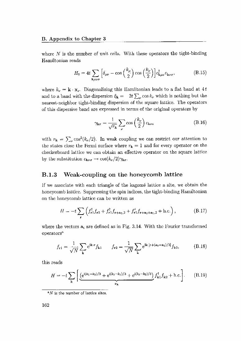
B. Appendix to Chapter 3
where N is the number of unit cells. With these operators the tight-binding
Hamiltonian reads
Ho = 4t Y [<V " cos (^) cos (D]cUw (B-!5)
where kv — k x^. Diagonalizing this Hamiltonian leads to a flat band at At
and to a band with the dispersion £k = —2t J^ cos kv which is nothing but the
nearest-neighbor tight-binding dispersion of the square lattice. The operators
of this dispersive band are expressed in terms of the original operators by
7k(7 = ——Ycos \f) Ck (B.16)V
with rk = ^„cos2^/^). In weak coupling we can restrict our attention to
the states close the Fermi surface where rt = 1 and for every operator on the
checkerboard lattice we can obtain an effective operator on the square lattice
by the substitution ckwa — cos(kl//2)-ykfT.
B.1.3 Weak-coupling on the honeycomb lattice
If we associate with each triangle of the kagomé lattice a site, we obtain the
honeycomb lattice. Suppressing the spin indices, the tight-binding Hamiltonian
on the honeycomb lattice can be written as
H = ~lE (A/« + /rl/r+a.,2 + /rWa^.2 + h.C.) , (B.17)r
where the vectors a^ are defined as in Fig. 3.14. With the Fourier transformed
operators*1
^V'
vwk
this reads
H = -tY (ei(fcl~fc3)/3 + ei(fc2"fcl)/3 + e^-W) /t / + h.c.l. (B.19)V i' ' J
Xk
*N is the number of lattice sites.
162

B.l. RG analysis
This Hamiltonian can be diagonalized as
k JJ=±1
with
7kP = ~t= (fki ~ peiipkfk2) Xk = \xk\e^. (B.21)
At half-filling, the Fermi surface reduces to the to points K = -K' = -47r(l, 0)/3a.
We have the relation
xK+k = wV^-*»^3 + uJto-W* + e^-W « ^(kx - iky) (B.22)
where the last approximation is the first non-vanishing order of k. We obtain
for the eigenstates close to K and K'
1
7K+k,p ~ —7= (/K+k,i - PKfK+k,2) (B.23)
7K'+k,p ~ -T= (/K'+k,l + pKfvL'+kï)
with kc — (kx + iky)/k.Let us now return again to the kagomé lattice and let us work with a new
BZ consisting of the two subzones Z and Z' around the points K and K' as
shown in Fig. B.l. We introduce the operators (ui — el27r//3)
k G Z (B.24)
/ki \1
/ ^ -u -1 \ / cki
/k2 =^ -1 w a,2 ck2 | kGZ' (B.25)
/k3 / V "I 1 1 / V Ck3
where the operators Cki are defined as in Eq. (3.60). This is just a transfor¬
mation to an orthonormal basis in which the kinetic energy is diagonal at the
points K and K'. The operators f]r+k3 and /K/+k 3create states in the top flat
band. Using exactly the same formulas as in Eq. (B.23) we can now define the
states 7K+k,p and 7K'+k,p for p — ±1 that are approximate eigenstates of the
kinetic energy close to K and K'. Therefore, the weakly interacting kagomé
lattice at 1/3-filling can be mapped to a weakly interacting honeycomb lattice.
163

B. Appendix to Chapter 3
Figure B.l: The zones Z and Z' are triangles around the points K and K'. They
form together a Brillouin zone.
Let us now look, to what kind of interaction a weak Coulomb repulsion on
the kagomé lattice corresponds on the honeycomb lattice. First of all we note
that for sufficiently small U, we can neglect Umklapp processes.15 We obtain
#mt = UYYnrmînrmt (B.26)m
— ^ 2\^ Z.^ Ck+q,mTCk'-q,mlCk'm|CkmTkk'q m
A+B=C+D A
= U Z_^ / j / JCA+k+a.mjCB+k'-a.m.\.CC+k',m.l.c£?+k.roT'
ABCD<E{K,K'} kk'q m
where in the last expression the sum over the momenta is restricted to the
triangle of the corresponding zone. With help of Eq. (B.24, B.25) we can
rewrite this expression in terms of the / operators and dropping the terms
involving the top band this amounts to doing the substitutions.
kez'
(B.27)
bFor the kagomé strip the Umklapp processes were very important, but in that case the
Ferrai points were connected by half of the reciprocal lattice vector, which is here not the
case.
Cki -> 73(^2/ki -/k2) Cki ->
73 (^/kl - /k2)
Ck2 — 75(/k2 - /kl) kGZ Ck2 —> 7j(/k2-/kl)Ck2 -+ ^(<^2/k2-/kl) Ck2 ~* 73(^^2 -/kl)
164
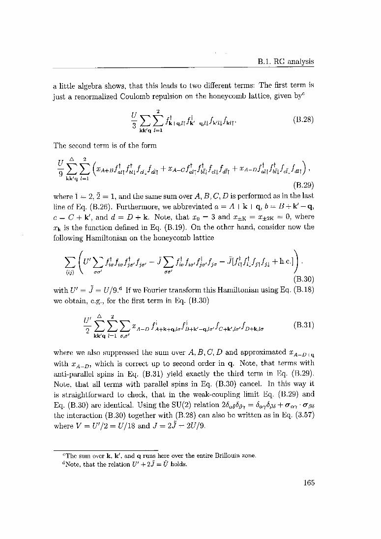
B.l. RG analysis
a little algebra shows, that this leads to two different terms: The first term is
just a renormalized Coulomb repulsion on the honeycomb lattice, given byc
U2
3" Z^ Z^ A:+q,Zî/k'-q,/|/k'ZJ./kZr (B.28)kk'q 1=1
The second term is of the form
A 2
U
~9 YY [XA+B-fanfbllfdlfdï1 + XA-C^al-[fbîifclifdï1 + XA-Dfalîfbîlfdlfdll) '
kk'q 1=1
(B.29)where ï = 2, 2 — 1, and the same sum over A, B, C, D is performed as in the last
line of Eq. (B.26). Furthermore, we abbreviated a — A + k + q, b = B + k' — q,
c — C + k', and d = D + k. Note, that x0 — 3 and z±k = £±2K — 0, where
xk is the function defined in Eq. (B.19). On the other hand, consider now the
following Hamiltonian on the honeycomb lattice
/ ,I"
2-^fiafiofja'fja' ~~ ^/^fiafia'fja'fjc ~ ^\fi\fijj\fj\ + n-c-]
{ij) \ aa' era'
(B.30)
with U' — 3 — U/9.d If we Fourier transform this Hamiltonian using Eq. (B.18)we obtain, e.g., for the first term in Eq. (B.30)
U'A 2
~9~ 2.^/ 2-^t 2^ XA-Ù JA+k+^laJB+k'-nJa'fc+k'ja'JD+kila (B.31)
kk'q 1=1 a,a'
where we also suppressed the sum over A, B, C, D and approximated xA_D+(l
with xA_D, which is correct up to second order in q. Note, that terms with
anti-parallel spins in Eq. (B.31) yield exactly the third term in Eq. (B.29).
Note, that all terms with parallel spins in Eq. (B.30) cancel. In this way it
is straightforward to check, that in the weak-coupling limit Eq. (B.29) and
Eq. (B.30) are identical. Using the SU(2) relation 28as8ß1 — 8ai8ßs + cra-y• &ß6
the interaction (B.30) together with (B.28) can also be written as in Eq. (3.57)
where V = U'/2 = U/18 and 3 - 23 = 2U/9.
cThe sum over k, k', and q runs here over the entire Brillouin zone.
dNote, that the relation U' + 2J = Ü holds.
165

Seite Leer /
Blank leaf

c
Appendix to Chapter 5
C.l Anderson bound for the energy
We consider the antiferromagnetic Heisenberg Hamiltonian
H = S0-Si + XS-S2 (C.l)
with A > 0, Si = S1(1 H + £>i,„x and S2 = S2,i + h S2,n2- Here, S0
and all Stj are spin-1/2 operators. The Hamiltonian H commutes with S2,
S\, S2, S2ot = (So + Si + S2)2, and with S*ot. We can therefore assume that
the ground state lies in a sector of the Hilbert space, where S1 — Si(Si + 1),
S22 = S2(S2 + 1), Sua = Stot(Stot + 1), and S^ = Stoi. Further, we know
that 5tot — (ni + n2 — l)/2 [155]. This leaves us with the following three
possibilities: Si — ni/2 — 1, S2 — n2/2, or Si — nx/2, S2 — n2/2 — 1, or
Si — ni/2, S2 — n2/2. In the first two cases the three spins S0, Si, and S2
must be parallel in order to produce St0t. This leads to a ferromagnetic state
which has positive energy. In the ground state we must therefore have the third
possibility, 5, = n\/2 and S2 = n2/2. In the 2(2ni + l)(2n2 + 1) dimensional
Hilbert space, given by the tensor product of the three spin representations,
we have only a three-dimensional subspace with S£ot = (ni + n2— l)/2. It is
straightforward to diagonalize the Hamiltonian in this subspace and the lowest
eigenvalue is given by:
E0 = ~ (1 + X + R) (C.2)
with
R= y/(l - X2)(l + ni)2 - 2A(1 - A)(l + n, + n2 - mn2) + X2(rn + n2)2.
167

C. Appendix to Chapter 5
The Hamiltonian (5.2) is the sum of Hamiltonians of the form (C.l). As the
sum of the minima can not be larger than the minimum of the sum, it is clear
that we obtain an upper bound by minimizing every Hamiltonian separately.
The equations (5.17) are now obtained from (C.2) with ni = 4, n2 = 2 and
A = r if N > 2, or with rii = A, n2 = 1 and A = 2r if N = 2. Note, that energy
per site is —e = E0/2.
C.2 Proof of Gaussian domination
For the Hamiltonian H+(ha) of (5.32) we can choose the planes perpendicular
to <53 to separate the Hilbert space into two equal Hilbert spaces corresponding
to the two layers. With respect to these planes the Hamiltonian iï"+(/ïa) takes
the form A +Ä+ ^Ct-Ci-K)2-T.j^j ~^jf and (5-33) follows therefore
directly from (5.28). To prove (5.33) for the Hamiltonian H~(ha) we define
the more general Hamiltonian H~(haj), which is given by (5.32) and (5.30) for
u = —, haj — haj, and d~ — haj. It depends on four fields and not only on
one and is therefore more general than H~(ha). We will show that
E[H-(h®)]>E[H-(0)] (C.3)
from which (5.33) for the Hamiltonian H~(ha) follows as a special case. We
denote by {ha^} a configuration of the 4|A| real fields and we will assume
that of all configurations that minimize E[H~(haj)] the configuration {haj}has the largest number of vanishing fields. If the configuration {h^'j} had a
non-vanishing field haj ^ 0, we could choose a pair of planes parallel to ö3,
that separate the lattice A into two equal subsystems in such a way that the
term containing haj in (5.30) connects the two subsystems. With respect to
these planes the Hamiltonian H~(haj) can be written in the form of (5.26)and we can apply (5.28). The Hamiltonians Ha and Hß can be written in the
form H~(aaj) and H~(baj) and therefore, due to our assumption, we must
have E[H-(W)} < E[H-'(a{^)} and E[H-(h^)] < E[H~(bal\)}. From (5.28)
follows now that E[H-(h[l])\ = E[H~(aal)j)} = E[H'(b^)]. The number of
vanishing fields is at least in one of the two configurations {aaj} and {bjj}strictly larger than in {ha'À, which contradicts the assumption that the number
of vanishing fields in {haj} is maximal. This shows that all the fields in {haj}must be zero and proves the inequality (C.3).
168
Bibliography
[1] E. Dagotto and T. M. Rice, Science 271, 618 (1996).
[2] K. S. Novoselov et ed., Science 306, 666 (2004).
[3] M. I. Katsnelson, K. S. Novoselov, and A. K. Geim, Nature Physics
(2006).
[4] G. W. Semenoff, Phys. Rev. Lett. 53, 2449 (1984).
[5] F. D. M. Haldane, Phys. Rev. Lett. 61, 2015 (1988).
[6] K. Takada et al, Nature 422, 53 (2003).
[7] B. Pedrini et al, Phys. Rev. B 72, 214407 (2005).
[8] M. E. Briihwiler, Groundstate Properties of Electrons on the Triangular
Lattice, PhD thesis, ETH Zürich, 2006.
[9] G. Misguich and C. Lhuillier, Frustrated spin systems, H.T.Diep editor,
World-Scientific, 2005, (cond-mat/0310405).
[10] J. Solyom, Adv. Phys. 28, 201 (1979).
[11] S. R. White, Phys. Rev. Lett. 69, 2863 (1992).
[12] B. Binz, D. Baeriswyl, and B. Doucot, Eur. Phys. J. B 25, 69 (2002).
[13] J. Gonzalez, F. Guinea, and M. A. H. Vozmediano, Nucl. Phys. B 424,
595 (1994).
[14] R. Shankar, Rev. Mod. Phys. 66, 129 (1994).
[15] M. Salmhofer, C. Honerkamp, W. Metzner, and O. Lauscher, Prog.Theor.
Phys. 112, 943 (2004).
169
Bibiliography
[16
[iT
[18
[19
[20
[21
[22
[23
[24
[25
[26
[27
[28;
[29
[30
[31
[32
[33
[34;
[35
170
H. H. Lin, L. Balents, and M. P. A. Fisher, Phys. Rev. B 58, 1794 (1998).
B. Frischmuth, PhD thesis, ETH Zürich, 1998.
P. Coleman, Phys. Rev. B 29, 3035 (1984).
F. C. Zhang and T. M. Rice, Phys. Rev. B 37, 3759 (1988).
I. Affleck, Z. Zou, T. Hsu, and P. W. Anderson, Phys. Rev. B 38, 745
(1988).
P. A. Lee and N. Nagaosa, Phys. Rev. B 46, 5621 (1992).
T. Tanaka, S. Nakamura, and S. Iida, Japn. J. Appl. Phys. 33, L581
(1994).
I. Terasaki, Y. Sasago, and K. Uchinokura, Phys. Rev. B 56, R12685
(1997).
Y. Wang, N. S. Rogado, R. J. Cava, and N. P. Ong, Nature 423, 425
(2003).
T. Valla et al, Nature 417, 627 (2002).
R, E. Schaak, T. Klimczuk, M. L. Foo, and R. J. Cava, Nature 424, 527
(2003).
M. L. Foo et al, Phys. Rev. Lett. 92, 247001 (2004).
Q. Huang et al, J.Phys.: Condens. Matter 16, 5803 (2004).
H. W. Zandbergen et al, Phys. Rev. B 70, 024101 (2004).
Y. G. Shi, H. C. Yu, C. J. Nie, and J. Q. Li, cond-mat/0401052 (2004).
X. Z. Chen et al, cond-mat/0412299 (2004).
Q. Huang et al, Phys. Rev. B 70, 184110 (2004).
N. L. Wang et al, Phys. Rev. Lett. 93, 237007 (2004).
R. Ray, A. Ghoshray, and K. Ghoshray, Phys. Rev. B 59, 9454 (1999).
J. L. Gavilano et al, Phys. Rev. B 69, 100404 (2004).

Bibiliography
[36] P. Carrctta et ed., Phys. Rev. B 70, 024409 (2004).
[37] M. Brühwiler, B. Batlogg, S. M. Kazakov, C. Niedermayer, and J. Karpin-
ski, Physica B: Condensed Matter 378-80, 630 (2006).
[38] C. Bernhard et al, Phys. Rev. Lett. 93, 167003 (2004).
[39] S. Lupi, M. Ortolani, and P. Calvani, Phys. Rev. B 69, 180506 (2004).
[40] L. Balicas, M. Abdel-Jawad, N. E. Hussey, F. C. Chou, and P. A. Lee,
Phys. Rev. Lett. 94, 236402 (2005).
[41] C. H. Wang et al, Solid State Commun. 138, 169 (2006).
[42] S. Lupi et al, Phys. Rev. B 72, 024550 (2005).
[43] I. R. Mukhamedshin, H. AUoul, G. Collin, and N. Blanchard, Phys. Rev.
Lett. 93, 167601 (2004).
[44] A. T. Boothroyd et al, Phys. Rev. Lett. 92, 197201 (2004).
[45] L. M. Helme et al, Phys. Rev. Lett. 94, 157206 (2005).
[46] Y. Ihara et al, J. Phys. Soc. Jpn. 73, 2963 (2004).
[47] T. Motohashi et al, Phys. Rev. B 67, 064406 (2003).
[48] B. C. Sales et al, Phys. Rev. B 70, 174419 (2004).
[49] J. Sugiyama et al, Phys. Rev. B 67, 214420 (2003).
[50] J. Sugiyama et al, Phys. Rev. Lett. 92, 017602 (2004).
[51] J. Wooldridge, D. M. Paul, G. Balakrishnan, and M. R. Lees, J. Phys.:
Condens. Matter 17, 707 (2005).
[52] F. C. Chou, J. H. Cho, and Y. S. Lee, Phys. Rev. B 70, 144526 (2004).
[53] G. Caimi et al, Eur. Phys. J. B 40, 231 (2004).
[54] J. L. Luo et al, Phys. Rev. Lett. 93, 187203 (2004).
[55] Y. J. Uemura et al, cond-mat/0403031 (2004).
[56] P. Mendels et al, Phys. Rev. Lett. 94, 136403 (2005).
171

Bibiliography
[57] D. J. Singh, Phys. Rev. B 61, 13397 (2000).
[58] G. Gasparovic et al, cond-mat/0508158 (2005).
[59] M. Yokoi et al, J. Phys. Soc. Jpn. 74, 3046 (2005).
[60] Y. Yanase, M. Mochizuki, and M. Ogata, J. Phys.Soc. Jpn. 74, 430 (2005).
[61] K. Miyoshi, E. Morikuni, K. Fujiwara, J. Takeuchi, and T. Hamasaki,
Phys. Rev. B 69, 132412 (2004).
[62] G. Baskaran, Phys. Rev. Lett. 91, 097003 (2003).
[63] B. Kumar and B. S. Shastry, Phys. Rev. B 68, 104508 (2003).
[64] A. Tanaka and X. Hu, Phys. Rev. Lett. 91, 257006 (2003).
[65] M. Ogata, J. Phys. Soc. Jpn. 72, 1893 (2003).
[66] Q.-H. W. D.-H. Lee and P. A. Lee, Phys. Rev. B 69, 092504 (2004).
[67] C. Honerkamp, Phys. Rev. B 68, 104510 (2003).
[68] A. Ferraz, E. Kochetov, and M. Mierzejewski, Phys. Rev. B 73, 064516
(2006).
[69] W. Koshibae and S. Maekawa, Phys. Rev. Lett. 91, 257003 (2003).
[70] M. Mochizuki, Y. Yanase, and M. Ogata, Phys. Rev. Lett. 94, 147005
(2005).
[71] D. J. Singh, Phys. Rev. B 68, 020503 (2003).
[72] M. D. Johannes, 1.1. Mazin, D. J. Singh, and D. A. Papaconstantopoulos,
Phys. Rev. Lett. 93, 097005 (2004).
[73] K.-W. Lee, J. Kunes, and W. E. Pickett, Phys. Rev. B 70, 045104 (2004).
[74] Z. Li, J. Yang, J. G. Hou, and Q. Zhu, Phys. Rev. B 71, 024502 (2005).
[75] P. Zhang, W. Luo, V. H. Crespi, M. L. Cohen, and S. G. Louie, Phys.
Rev.B 70, 085108 (2004).
[76] P. Zhang, R. B. Capaz, M. L. Cohen, and S. G. Louie, Phys. Rev. B 71,
153102 (2005).
172
Bibiliography
[77] M. D. Johannes, I. I. Mazin, and D. J. Singh, Phys. Rev. B 71, 205103
(2005).
[78
[79
[80
[81
[82
[83
[84
[85
[86;
[87
[88;
[89
[90
[91
[92
[93
[94
[95
M. Z. Hasan et al, Phys. Rev. Lett. 92, 246402 (2004).
H.-B. Yang et al, Phys. Rev. Lett. 92, 246403 (2004).
H.-B. Yang et al, cond-mat/0501403 (2005).
D. Qian et al, Phys. Rev. Lett. 96, 046407 (2006).
D. Qian et al, Phys. Rev. Lett. 96, 216405 (2006).
W. B. Wu et al, cond-mat/0408467 (2004).
M. Indergand, Y. Yamashita, H. Kusunose, and M. Sigrist, Phys. Rev. B
71, 214414 (2005).
M. Indergand and M. Sigrist, Phys. B: Condens. Matter 359-361, 1357
(2005).
Y. Imai, N. Kawakami, and H. Tsunetsugu, Phys. Rev. B 68, 195103
(2003).
A. Läuchli and D. Poilblanc, Phys. Rev. Lett. 92, 236404 (2004).
D. Poilblanc, Phys. Rev. Lett. 93, 197204 (2004).
N. Bulut, W. Koshibae, and S. Maekawa, Phys. Rev. Lett. 95, 037001
(2005).
E. Runge and P. Fulde, Phys. Rev. B 70, 245113 (2004).
S. Kondo et al, Phys. Rev. Lett. 78, 3729 (1997).
S. H. Lee, Y. Qiu, C. Broholm, Y. Ucda, and J. J. Rush, Phys. Rev. Lett.
86, 5554 (2001).
L. Santos et al, Phys. Rev. Lett. 93, 030601 (2004).
B. Damski et al, Phys. Rev. Lett. 95, 060403 (2005).
C. L. Henley, Can. J. Phys. 79, 1307 (2001).
173
Bibiliography
[96] M. Indergand, A. Läuchli, S. Capponi, and M. Sigrist, Phys. Rev. B 74,
064429 (2006).
[97] M. Indergand, C. Honerkamp, A. Läuchli, D. Poilblanc, and M. Sigrist,
cond-mat/0609129 (2006).
[98] T. Koretsune and M. Ogata, J. Phys. Soc. Jpn. 72, 2437 (2003).
[99] C. J. Morningstar and M. Weinstein, Phys. Rev. D 54, 4131 (1996).
[100] S. Capponi, A. Läuchli, and M. Mambrini, Phys. Rev. B 70, 104424
(2004).
[101] E. Berg, E. Altman, and A. Auerbach, Phys. Rev. Lett. 90, 147204 (2003).
[102] R. Budnik and A. Auerbach, Phys. Rev. Lett. 93, 187205 (2004).
[103] R. Moessner, S. L. Sondhi, and M. O. Goerbig, Phys. Rev. B 73, 094430
(2006).
[104] S. Sorella and E. Tosatti, Europhys. Lett. 19, 699 (1992).
[105] L. M. Martelo, M. Dzierzawa, L. Siffert, and D. Baeriswyl, Z. Phys. B
Condens. Matter 103, 335 (1997).
[106] J. Gonzalez, F. Guinea, and M. A. H. Vozmediano, Phys. Rev. B 6313,
134421 (2001).
[107] F. C. Zhang, C. Gros, T. M. Rice, and H. Shiba, Supercond.Sci.Technol.
1, 36 (1988).
[108] V. Yushankhai, P. Fulde, and P. Thalmeier, Phys. Rev. B 71, 245108
(2005).
[109] C. Waldtmann, H. Kreutzmann, U. Schollwock, K. Maisinger, and H. U.
Everts, Phys. Rev. B 62, 9472 (2000).
[110] R. Moessner, O. Tchernyshyov, and S. Sondhi, J. Stat. Phys. 116, 755
(2004).
[111] B. Canals, Phys. Rev. B 65, 184408 (2002).
[112] J.-B. Fouet, M. Mambrini, P. Sindzingre, and C. Lhuillier, Phys. Rev. B
67, 054411 (2003).
174

Bibiliography
[113] W. Brenig and A. Honecker, Phys. Rev. B 65, 140407 (2002).
[114] H. B. Nielsen and M. Ninomiya, Nucl. Phys. B 193, 173 (1981).
[115] H. B. Nielsen and M. Ninomiya, Nucl. Phys. B 185, 20 (1981).
[116] R. Jackiw, Phys. Rev. D 29, 2375 (1984).
[117] P. W. Anderson, Science 235, 1196 (1987).
[118] M. P. A. Fisher, Topological Aspects of Low Dimensional Systems, Session
LXIX, EDP Sciences, 1998.
[119] T. Timusk and B. Statt, Rep. Prog. Phys. 62, 61 (1999).
[120] R. Coldea, D. A. Tennant, A. M. Tsvelik, and Z. Tylczynski, Phys. Rev.
Lett. 86, 1335 (2001).
[121] M. Azuma, Z. Hiroi, M. Takano, K. Ishida, and Y. Kitaoka, Phys. Rev.
Lett. 73, 3463 (1994).
[122] E. Dagotto, J. Riera, and D. Scalapino, Phys. Rev. B 45, 5744 (1992).
[123] T. M. Rice, S. Goplan, and M. Sigrist, Europhys. Lett. 23, 445 (1993).
[124] C. A. Hayward, D. Poilblanc, R. M. Noack, D. J. Scalapino, and
W. Hanke, Phys. Rev. Lett. 75, 926 (1995).
[125] M. Troyer, H. Tsunetsugu, and T. M. Rice, Phys. Rev. B 53, 251 (1996).
[126] L. Balents and M. P. A. Fisher, Phys. Rev. B 53, 12133 (1996).
[127] K. L. Hur, Phys. Rev. B 64, 060502 (2001).
[128] E. Dagotto, Rep. Prog. Phys. 62, 1525 (1999).
[129] M. Uehara et al, J. Phys. Soc. Jpn. 65, 2764 (1996).
[130] C. H. Ahn et al, Science 276, 1100 (1997).
[131] C. H. Ahn et al, Science 284, 1152 (1999).
[132] S. Gariglio, C. H. Ahn, D. Matthey, and J. M. Triscone, Phys. Rev. Lett.
88, 067002 (2002).
175
Bibiliography
[133
[134;
[135
[136
[137
[138
[139
[140
[141
[142
[143
[144
[145;
[146
[147
[148
[149
[150
[151
[152
[153
176
Z. Hiroi and M. Takano, Nature 377, 41 (1995).
S. Wcssel, M. Indergand, A. Läuchli, U. Ledermann, and M. Sigrist, Phys.
Rev.B 67, 184517 (2003).
M. Sigrist, T. M. Rice, and F. C. Zhang, Phys. Rev. B 49, 12058 (1994).
H. H. Lin, L. Balents, and M. P. A. Fisher, Phys. Rev. B 56, 6569 (1997).
U. Ledermann, K. L. Hur, and T. M. Rice, Phys.Rev.B 62, 16383 (2000).
F. D. M. Haldane, J.Phys.C: Solid State Phys. 14, 2585 (1981).
H. J. Schulz, Proceedings of Les Houches Summer School LXI, Elsevier
Amsterdam, 1995.
T. M. Rice, S. Haas, M. Sigrist, and F. C. Zhang, Phys. Rev. B 56, 14655
(1997).
M. U. Ubbens and P. A. Lee, Phys. Rev. B 46, 8434 (1992).
G. Kotliar and J. L. Liu, Phys. Rev. B 38, 5142 (1988).
C. Honerkamp and P. A. Lee, Phys. Rev. Lett. 90, 246402 (2003).
T. Matsuda and K. Hida, J. Phys. Soc. Jpn. 59, 2223 (1990).
K. Hida, J. Phys. Soc. Jpn. 61, 1013 (1992).
J. Fröhlich, B. Simon, and T. Spencer, Comm. Math. Phys. 50, 79 (1976).
J. Fröhlich, B. Simon, and T. Spencer, Phys. Rev. Lett. 36, 804 (1976).
F. J. Dyson, E. H. Lieb, and B. Simon, J. Stat. Phys. 18, 335 (1978).
I. Affleck, T. Kennedy, E. H. Lieb, and H. Tasaki, Comm. Math. Phys.
115, 477 (1988).
E. J. Nevcs and J. F. Perez, Phys. Lett. A 114, 331 (1986).
T. Kennedy, E. H. Lieb, and B. S. Shastry, J.Stat.Phys.53, 1019 (1988).
K. Kubo and T. Kishi, Phys. Rev. Lett. 61, 2585 (1988).
Y. Ozcki, H. Nishimori, and Y. Tomita, J. Phys. Soc. Jpn. 58, 82 (1988).
Bibiliography
[154] J. R. Parreira, 0. Bolina, and J. F. Perez, J.Stat. Phys. 86, 1367 (1997).
[155] E. H. Lieb and D. Mattis, J. Math. Phys. 3, 749 (1962).
[156] T. Kishi and K. Kubo, J. Phys. Soc. Jpn. 58, 2547 (1989).
[157] J. P. Serre, Linear Representations of Finite Groups, Springer-Verlag,
New York, 1977.
[158] J. 0. Fjaerestad and J. B. Marston, Phys. Rev. B 65, 125106 (2002).
[159] M. Tsuchiizu and A. Furusaki, Phys.Rev.B 66, 245106 (2002).
177
Seite Leer /
Blank leaf

Acknowledgments
First of all I would like to express my gratitude to my supervisor Manfred Sigrist
for accepting me as a student. During the numerous discussions with him I
could profit enormously from his deep insights and his broad overview on solid
state physics. His friendly and humorous personality provided an enjoyable
working atmosphere that I appreciated a lot. I am also deeply indepted to my
co-examiner Andreas Läuchli. Already during my diploma thesis he supported
me with his advice and also during my PhD time we continued to collaborate
in a fruitful and enjoyable way. Apart from work I could also count on Andreas
as a reliable table-soccer or mountaineering partner. Many thanks also go to
Carsten Honerkamp who as a young father found time to read my thesis and
agreed to be my co-examiner.
I enjoyed to share the office with two dynasties of postdocs. On one hand
there was the Japanese dynasty with Hiro, Yasu, Waka, and Hirono and on
the other hand the Spanish-German dynasty with Klaus, Leni, Sebastian, and
Christian. I could profit a lot from their experience and I would probably even
have learned Japanese, if I had stayed much longer in this office. But also out¬
side of the office I could discuss with experienced people like Beni, Benedikt,
Christian, Dima, Matthias, Masa, Stefan, Urs, and Youichi. Particularly in¬
teresting where the discussions with the experimentalists Markus Brühwiler,
Betram Batlogg, Bill Pedrini and Jorge Gavilano about the cobaltates.
I believe that it is sufficient to thank my friends who did their PhD together
with me only with a few words, as they surely know how grateful I am for the
beautiful time we spent together. In particular my thanks go to: Jerome and
Kathi, whose friendship already dates back to an ERASMUS exchange in Spain
and survived several years of flatsharing. Samuel, Barbara, and Martin with
whom I climbed steep walls and skied white powder-slopes. Igor i Renata, koji
su me pozvali na Hvar i koji su pricali srpsko-hrvatski sa mnom. Alvise, Chiara,
and Paolo who embellished our lives with delicious food or simply with their
179

Italianità.
Towards the end of my thesis I got to know more and more PhD students
of the younger generation like Andreas Schnyder, Sebastian, Fabian, Andreas
Rüegg, Alexander, and Mark who seem to be quite cool as well. With An¬
dreas and Mark I had the pleasure to collaborate while they were writing their
diploma thesis in the group of Manfred Sigrist. Of course, special thanks belong
to Fabian, who as my new flatmate was a worthy successor of Jerome.
Before finishing, I want to express my thanks to Dirk Manske for Badminton
and Berlin, to all members of the VAK for the cool ski-tours and to Serge and
Eugénie for all the funny weekend trips around Karlsruhe.
Last but not least I am very grateful to my parents who supported me
during the whole time of my studies. I always could find a beautiful warm
home in Andermatt if I wanted to escape the busy life of Zurich. Finally, I
thank my Marijana for everything she did for me.
180

Curriculum Vitae
Persönliche Daten
Name:
Geburtsdatum:
Nationalität:
Martin Franz Indergand
21. Februar 1975
Schweizer
Ausbildung
1982-1988
1988-1995
Primarschule Andermatt
Gymnasium an der Klosterschule Disentis
1996-2001
1998-1999
2001
Physikstudium an der ETH Zürich
Erasmus-Studienjahr in Granada, Spanien
Diplomarbeit an der ETH Zürich
bei Prof. Manfred Sigrist
2002-2006 Dissertation am Institut für Theoretische Physik
der ETH Zürich bei Prof. Manfred Sigrist
181