orbit and bulk density of the osiris-rex target asteroid ... · da=dt= ( 19:0 0:1) 10 4 au/myr or...
TRANSCRIPT

Accepted by Icarus on February 19, 2014
Orbit and Bulk Density of the OSIRIS-REx Target Asteroid (101955) Bennu
Steven R. Chesley∗1, Davide Farnocchia1, Michael C. Nolan2, David Vokrouhlicky3, Paul W.
Chodas1, Andrea Milani4, Federica Spoto4, Benjamin Rozitis5, Lance A. M. Benner1, William F.
Bottke6, Michael W. Busch7, Joshua P. Emery8, Ellen S. Howell2, Dante S. Lauretta9, Jean-Luc
Margot10, and Patrick A. Taylor2
ABSTRACT
The target asteroid of the OSIRIS-REx asteroid sample return mission, (101955)
Bennu (formerly 1999 RQ36), is a half-kilometer near-Earth asteroid with an extraor-
dinarily well constrained orbit. An extensive data set of optical astrometry from
1999–2013 and high-quality radar delay measurements to Bennu in 1999, 2005, and
2011 reveal the action of the Yarkovsky effect, with a mean semimajor axis drift rate
da/dt = (−19.0 ± 0.1) × 10−4 au/Myr or 284 ± 1.5 m/yr. The accuracy of this result
depends critically on the fidelity of the observational and dynamical model. As an ex-
ample, neglecting the relativistic perturbations of the Earth during close approaches
affects the orbit with 3σ significance in da/dt.
The orbital deviations from purely gravitational dynamics allow us to deduce the
acceleration of the Yarkovsky effect, while the known physical characterization of Bennu
allows us to independently model the force due to thermal emissions. The combination
of these two analyses yields a bulk density of ρ = 1260 ± 70 kg/m3, which indicates a
macroporosity in the range 40± 10% for the bulk densities of likely analog meteorites,
1Jet Propulsion Laboratory, California Institute of Technology, 4800 Oak Grove Drive, Pasadena, CA 91109, USA
2Arecibo Observatory, Arecibo, PR, USA
3Charles Univ., Prague, Czech Republic
4Univ. di Pisa, Pisa, Italy
5Open Univ., Milton Keynes, UK
6Southwest Research Institute, Boulder, CO, USA
7SETI Inst., Mountain View, CA, USA
8Univ. Tennessee, Knoxville, TN, USA
9Univ. Arizona, Tucson, AZ, USA
10Univ. California, Los Angeles, CA, USA
arX
iv:1
402.
5573
v1 [
astr
o-ph
.EP]
23
Feb
2014

– 2 –
suggesting a rubble-pile internal structure. The associated mass estimate is (7.8±0.9)×1010 kg and GM = 5.2± 0.6 m3/s2.
Bennu’s Earth close approaches are deterministic over the interval 1654–2135, be-
yond which the predictions are statistical in nature. In particular, the 2135 close ap-
proach is likely within the lunar distance and leads to strong scattering and therefore
numerous potential impacts in subsequent years, from 2175–2196. The highest individ-
ual impact probability is 9.5 × 10⁻⁵ in 2196, and the cumulative impact probability is
3.7× 10⁻⁴, leading to a cumulative Palermo Scale of -1.70.
Subject headings: Near-Earth objects; Orbit determination; Celestial mechanics; Yarkovsky
Effect; Impact Hazard
1. Introduction
The Apollo asteroid (101955) Bennu, a half-kilometer near-Earth asteroid previously desig-
nated 1999 RQ36, is the target of the OSIRIS-REx sample return mission. A prime objective of
the mission is to measure the Yarkovsky effect on this asteroid and constrain the properties that
contribute to this effect. This objective is satisfied both by direct measurement of the accelera-
tion imparted by anisotropic emission of thermal radiation, the first results of which are reported
here, and by constructing a global thermophysical model of the asteroid to confirm the underlying
principles that give rise to this effect.
Bennu was discovered by the LINEAR asteroid survey in September 1999. Since then, more
than 500 optical observations have been obtained for this Potentially Hazardous Asteroid (PHA).
Moreover, the asteroid was observed using radar by the Arecibo and Goldstone radio telescopes
during three different apparitions. Thanks to this rich observational data set, Bennu has one of
the most precise orbits in the catalog of known near-Earth asteroids. The exceptional precision
of the Bennu orbit allows one to push the horizon for predicting possible Earth impacts beyond
the 100 years typically used for impact monitoring (Milani et al. 2005), and indeed Milani et al.
(2009) showed that Earth impacts for Bennu are possible in the second half of the next century.
In particular, the cumulative impact probability they found was approximately 10−3, about half of
which was associated with a possible impact in 2182. However, the occurrence of an impact depends
decisively on the Yarkovsky effect because the prediction uncertainty due to this nongravitational
perturbations dominates over the orbital uncertainty associated with astrometric errors.
The Yarkovsky effect is a subtle nongravitational perturbation that primarily acts as a secular
variation in semimajor axis and thus causes a runoff in orbital anomaly that accumulates quadrat-
ically with time (Bottke et al. 2006). The computation of the Yarkovsky perturbation requires a
rather complete physical model of the asteroid, including size, shape, density, spin rate and orien-
tation, thermal properties, and even surface roughness (Rozitis and Green 2012). Though such a
complete profile is rarely available, the orbital drift due to the Yarkovsky effect can sometimes be

– 3 –
determined from an asteroid observational data set. For example, Chesley et al. (2003) managed to
directly estimate the Yarkovsky effect for asteroid (6489) Golevka by using three radar apparitions.
Vokrouhlicky et al. (2008) employ the Yarkovsky effect to match precovery observations of asteroid
(152563) 1992 BF that are incompatible with purely gravitational dynamics. More recently Nugent
et al. (2012) and Farnocchia et al. (2013b) have estimated the Yarkovsky effect for a few tens of
near-Earth asteroids by using a formulation that depends on a single parameter to be determined
from the orbital fit.
Besides Bennu, there are two other asteroids for which possible impacts are known to be driven
by the Yarkovsky effect: (29075) 1950 DA (Giorgini et al. 2002) and (99942) Apophis (Chesley 2006;
Giorgini et al. 2008). The relevance of the Yarkovsky effect for Apophis is due to a scattering close
approach in 2029 with minimum geocentric distance ∼38000 km. For 1950 DA the influence of
the Yarkovsky effect for an impact in 2880 is due to the long time interval preceding the potential
impact. However, no estimate of the Yarkovsky perturbation acting on these two asteroids is
currently available. To analyze such cases one can use the available physical constraints for the
specific objects, along with general properties of near-Earth asteroids (e.g., albedo, thermal inertia,
bulk density, etc.) to statistically model the Yarkovsky effect. The orbital predictions and the
impact hazard assessment are then performed by a Monte Carlo simulation that accounts for both
the Yarkovsky effect distribution and the orbital uncertainty (Farnocchia et al. 2013a; Farnocchia
and Chesley 2014). For Bennu, no such heroics are required. As we shall see, we now have a precise
estimate of the orbital deviations caused by the Yarkovsky effect, as well as a comprehensive physical
model distilled from numerous investigations.
While the Yarkovsky effect requires a priori knowledge of several physical parameters to be
computed directly, its detection through orbital deviations can be used to constrain the otherwise
unknown physical parameters. When the spin state is unknown, one can derive weak constraints
on obliquity, as was first shown by Vokrouhlicky et al. (2008) for 1992 BF. In cases where the
spin state is well characterized, usually through the combination of radar imaging and photometric
light curves, the bulk density of the object is correlated with the thermal properties and mutual
constraints can be inferred, as was the case for Golevka (Chesley et al. 2003). Rozitis et al.
(2013) were able to jointly model the measured Yarkovsky and YORP effects on (1862) Apollo,
and thereby constrain a number of the body’s physical characteristics, including axis ratios, size,
albedo, thermal inertia and bulk density. In the case of Bennu, the thermal inertia is known from
infrared observations (Emery et al. 2014; Muller et al. 2012), and so we are able to directly estimate
the mass and bulk density.

– 4 –
2. Observational Data and Treatment
2.1. Optical Astrometry
We use the 569 RA-DEC astrometric measurements available from the Minor Planet Center
from 1999-Sep-11.4 to 2013-Jan-20.1. We apply the star catalog debiasing algorithm introduced by
Chesley et al. (2010), and data weights are generally based on the astrometric weighting scheme
proposed in Sec. 6.1 of that paper. In some cases there is an excess of observations from a single
observatory in a single night. In such cases we relax the weights by a factor of about√N/5, where
N is the number of observations in the night. This reduces the effect of the particular data set to
a level more consistent with the typical and preferred contribution of 3–5 observations per night.
Considerable care was taken in identifying outlier observations to be deleted as discordant with
the bulk of the observations. From among the 569 available observations from 43 stations, we reject
91 as outliers, leaving 478 positions from 34 stations in the fits. Figure 1 depicts the postfit plane
of sky residuals, highlighting the deleted data. There are an additional 14 observations, all deleted,
that are not depicted in Fig. 1 because they fall beyond the limits of the plot. The manual rejection
approach often deletes an entire batch of data if it appears biased in the mean, thus some of the
deleted points in Fig. 1 do not show significant residuals. On the other hand, some observations
are de-weighted relative to the others, and in some cases these are not deleted, despite the raw
residuals being larger than some rejected observations. In Sec. 3.4 we discuss the dependency of
the ephemeris prediction on the outlier rejection approach.
[Figure 1 about here.]
2.2. Radar Astrometry
The time delay and Doppler shift of radar echoes from Bennu were measured in 1999, 2005
and 2011. Radar astrometry was obtained at both Arecibo and Goldstone as detailed in Table 1.
The delay observations in the table correspond to the round-trip light travel time from the nominal
telescope position to the center of mass of the object, and thus they are often referred to as range
measurements. Doppler measurements in the table reflect the frequency shift between the transmit
and receive signals due to the line-of-sight velocity of the object. The use of radar delay and
Doppler measurements in asteroid orbit determination was introduced by Yeomans et al. (1992).
Delay uncertainties arise from the finite resolution of the imaging of 0.05-0.125 µs/px (Nolan
et al. 2013), uncertainty in the shape modeling (to determine the center of mass from the observed
echo power) of 10-20 m, equivalent to about 0.1 µs, and systematic calibration, including uncertain-
ties in the position of the telescope and light travel within the telescope optics. Because we have a
shape model of Bennu that directly relates the individual range observations to the center of figure
of the model (Nolan et al. 2013), the systematic uncertainties dominate the range uncertainty in the

– 5 –
1999 and 2005 observations, and are assigned conservative values of 1.0 and 0.5 µs (respectively).
In 2011, Bennu was much farther away than the previous observations, and the uncertainty of 2 µs
is from the pixel scale of the observations. Doppler uncertainties are taken to be 1 Hz at 2380 MHz,
about 1/4 of the total rotational Doppler width of the object, and are based on the uncertainty of
estimating the position of the center of mass of the spectra.
The 2011 observations (Fig. 2 and Table 2) were of too low resolution and SNR to be useful for
shape modeling and were obtained solely for improving our knowledge of the orbit of Bennu. The
2-µs (300 m) resolution was chosen to be the finest resolution that would maximize the SNR of the
observations by including all of the echo power from the 250-m radius asteroid in one or two range
bins. The asteroid was visible with a SNR > 3 on each of the three observing dates at consistent
delay and Doppler offsets from the a priori ephemeris used in the data taking.
The 2011 radar observations of Bennu, which enabled the results of the present paper, almost
never happened. The two-million-Watt, 65,000-Volt “power brick” that supplies the electricity for
the Arecibo Planetary Radar system failed in late 2010, and was finally repaired on September
15, 2011. Because of the critical schedule for Bennu observations, in a space of seven days the
16-ton unit was trucked 800 miles from Pennsylvania to Florida, shipped to Puerto Rico, trucked
again, and lifted into place with a crane. The system was reconnected and recommissioned in four
days, after nearly a year of down-time, just in time to perform the observations on the last possible
dates of September 27–29, and just as the prime contractor managing the Arecibo Observatory was
changing (on October 1), after 45 years of operation by Cornell University, so that most observatory
operations were frozen for the transition.
[Figure 2 about here.]
[Table 1 about here.]
[Table 2 about here.]
3. Orbit Determination and Dynamical Model
We have updated the orbit determination for Bennu based on the observational data set de-
scribed above. These orbital position measurements place extraordinary constraints on the orbit
determination, and thus we must pay careful attention to the fidelity of force models, observation
models and numerical integration. Our dynamical model includes direct solar radiation pressure
and the thermal re-emission of absorbed solar radiation (i.e., the Yarkovsky effect). Besides the
gravitational acceleration of the Sun, we include Newtonian perturbations by the eight planets, the
Moon, Pluto and 25 selected main belt asteroids. We consider the oblateness term of the Earth’s
geopotential and full relativistic perturbations from the Sun, eight planets and the Moon.

– 6 –
As shown by Giorgini et al. (2002), who studied the potential impact of 29075 (1950 DA) in
the year 2880, other potential dynamical perturbations, such as galactic tide, solar mass loss and
solar oblateness, are too slight to affect our results. This is because these small effects, which were
not important for 1950 DA, will be even less significant for Bennu due to the much shorter time
interval.
3.1. Yarkovsky Effect
The Yarkovsky effect is a key consideration when fitting an orbit for Bennu (Milani et al.
2009). This slight nongravitational acceleration arises from the anisotropic re-emission at thermal
wavelengths of absorbed solar radiation (Bottke et al. 2006). The component of the thermal recoil
acceleration in the transverse direction acts to steadily increase or decrease the orbital energy,
leading to a drift in semimajor axis da/dt that accumulates quadratically with time in the orbital
longitude of the asteroid. For a uniform, spherical asteroid on a known orbit, the drift rate depends
on the physical characteristics of the asteroid according to
da
dt∝ cos γ
ρD,
where γ is the obliquity of the asteroid equator with respect to its orbital plane, ρ is the bulk
density of the asteroid, and D is the effective diameter. Additionally, da/dt depends in a nonlinear
and often nonintuitive way on the asteroid rotation period P and the surface material properties,
namely thermal inertia Γ, infrared emissivity ε and Bond albedo A (Vokrouhlicky et al. 2000).
We have three models available to us for computing thermal accelerations on Bennu. The first,
and most straightforward, is to simply apply a transverse acceleration of the form AT × (r/1 au)−d,
where AT is an estimable parameter, r is the heliocentric distance and the exponent is typically
assumed as d = 2 to match the level of absorbed solar radiation. Given an estimated value of ATand the assumed value of d, one can readily derive the time-averaged da/dt using Gauss’ planetary
equations (Farnocchia et al. 2013b). This approach, which we term the transverse model, is com-
putationally fast and captures the salient aspects of the thermal recoil acceleration. Importantly, it
requires no information about the physical characteristics or spin state of the asteroid, and so it can
be implemented readily in cases where only astrometric information is available (e.g., Vokrouhlicky
et al. 2008; Chesley et al. 2008; Nugent et al. 2012; Farnocchia et al. 2013b).
For Bennu we find numerically that the exponent d = 2.25 provides the best match to the
transverse thermal acceleration derived from the thermal re-emission models described below. This
result can also be computed analytically using a simplified model with the technique described in
Appendix A. Using the transverse model with d = 2.25 we derive JPL solution 87 (Table 3), which
serves as a reference solution as we investigate the effect of various model variations on the orbit.
JPL solution 87 yields a Yarkovsky drift estimate that compares well with the corresponding
result from Milani et al. (2009), who used observations only through mid-2006 and found da/dt =

– 7 –
(−15 ± 9.5) × 10−4 au/Myr, which was judged to be a weak detection of the nongravitational
acceleration. Using the same fit span (1999–2006) from the current data set we now find da/dt =
(−22.9 ± 5.3) × 10−4 au/Myr. The change in the estimate relative to that of Milani et al. (2009)
is due in large part to the use of star catalog debiasing (Chesley et al. 2010), while the improved
precision is due to the higher accuracy and quantity of radar delay measurements obtained through
re-measurement of the 1999 and 2005 Arecibo observations, as well through as the use of tighter
weights on the optical data proposed by Chesley et al. (2010). Incorporating the subsequent optical
observations through 2013 leads to da/dt = (−21.3± 4.6)× 10−4 au/Myr. Finally, adding the 2011
Arecibo radar astrometry reduces the uncertainty by nearly a factor 50, leading to the current best
estimate da/dt = (−19.0± 0.1)× 10−4 au/Myr. We note that the new formal uncertainty on da/dt
is 0.5%, by far the most precise Yarkovsky estimate available to date. As well, the uncertainty on
the semimajor axis a is 6 m, the lowest value currently found in the asteroid catalog. This low
uncertainty is primarily a reflection of the current precision of the orbital period (2 ms) rather than
an indication of the uncertainty in the predicted asteroid position, which is at the level of a few
kilometers during the fit span.
[Table 3 about here.]
Both our second (linear) and third (nonlinear) Yarkovsky acceleration models employ heat
transfer models of different levels of fidelity in order to predict the surface temperature and asso-
ciated re-emission of thermal energy. The linear model utilizes linearized heat transfer equations
on a rotating homogeneous sphere, closely following the development given by Vokrouhlicky et al.
(2000) for both the diurnal and seasonal components of the Yarkovsky effect. The linear model
requires knowledge of the spin orientation and rate, asteroid diameter and thermal inertia, but does
not allow for shape effects such as self-shadowing and self-heating, which are generally considered
minor. The linear model assumes a sphere, and so oblateness effects are not captured. This is
relevant because the cross-sectional area receiving solar radiation is increased for an equal volume
sphere relative to that of an oblate body, and thus the force derived with the linear model is en-
hanced relative to the nonlinear model. This in turn leads to an increased estimate of the bulk
density as we shall see later.
The nonlinear model is the highest fidelity Yarkovsky force model that we apply to the orbit
determination problem. This approach solves the nonlinear heat transfer equation on a finite-
element mesh of plates or facets that models the Nolan et al. (2013) asteroid shape. The approach
is described in more detail by Capek and Vokrouhlicky (2005), but we summarize it here. For each
facet on the asteroid shape model, the nonlinear heat transfer problem is solved while the asteroid
rotates with a constant spin rate and orientation and revolves along a frozen, two-body heliocentric
orbit. A uniform temperature distribution is assumed at start-up and the temperature and energy
balance between absorbed, conducted and re-radiated radiation for each facet is solved as a function
of time. The heat transfer problem is treated as one-dimensional, i.e., the temperature for a given
facet depends only on the depth below the facet. There is no conduction across or between facets.

– 8 –
After several orbital revolutions the temperature profile from revolution to revolution converges for
each plate. Following convergence, diurnal averaging of the vector sum of the thermal emission over
the body yields the force of thermal emission as a function of orbital anomaly. Given the shape
model volume and an assumed bulk density, the mass can be computed and from this the thermal
recoil acceleration. This ultimately leads to a lookup table of acceleration as a function of true
anomaly that is interpolated during the high-fidelity orbital propagation.
The nonlinear model was previously used with asteroid (6489) Golevka (Chesley et al. 2003),
but at that time the acceleration table was for a frozen orbit, which turns out to be an unacceptable
approximation for Bennu. Figure 3 shows the orbital element variations into the future due to
planetary perturbations and Fig. 4 reveals the associated variation in the average da/dt, which is
clearly significant relative to the 0.10 × 10⁻⁴ au/Myr uncertainty. As a result of this analysis we
have implemented an enhancement to the nonlinear model that corrects the tabulated accelerations
for variations in orbital elements. The approach is to compute the Yarkovsky force vector from a
linearized expansion about a central, reference orbit according to
~FY (a, e; fi) = ~FY (a0, e0; fi) +∂ ~FY (a0, e0; fi)
∂a(a− a0) +
∂ ~FY (a0, e0; fi)
∂e(e− e0).
Here ~FY is the thermal acceleration in the orbit plane frame so that variations of the Keplerian
Euler angle orbital elements (ω, Ω, i) do not affect the computation; ~FY is rotated to the inertial
frame during the propagation. The fi are the true anomaly values in the tabulation, a0 and e0are the values for the reference orbit. The partial derivatives are also tabulated after they are
derived by finite differences based on a series of pre-computed lookup tables for varying orbits~FY (a0 ± δa, e0 ± δe; fi).
[Figure 3 about here.]
[Figure 4 about here.]
When computing an orbit with the linear or nonlinear model we use the physical parameters
listed in Table 4, and for the nonlinear model we also use the Nolan et al. (2013) shape model.
The bulk density ρ is estimated as a free parameter. Because the semimajor axis drift da/dt is
constrained by the observations at the 0.5% level, any variations in the force computed by the
thermal models manifests as a variation in the estimated bulk density. This is discussed in greater
detail in Sec. 4.
[Table 4 about here.]
[Figure 5 about here.]

– 9 –
[Figure 6 about here.]
JPL solution 85 (Table 3) uses the nonlinear model, and is assumed to be our most accurate
orbital solution. To indicate the differences between the two models, Fig. 5 depicts the estimated
thermal recoil accelerations from the nonlinear and linear models. The plot reveals an excellent
agreement between the two models in the transverse acceleration, which is to be expected since the
transverse component is constrained by the observed orbital runoff and the associated semimajor
axis drift. The radial and normal (out-of-plane) accelerations show a good but imperfect agreement,
with linear model accelerations being noticeably reduced relative to the nonlinear model.
Figure 6 shows how the radial and transverse accelerations in the linear model affect the in-
stantaneous and average values of da/dt, as derived from the classical Gauss planetary equations.
During a given orbit, the variations in the instantaneous drift rate are much larger from the trans-
verse component. The normal component of acceleration does not affect the semimajor axis. While
the radial component of acceleration does lead to variations in semimajor axis during an orbital
period, in the mean the radial term does not contribute to semimajor axis drift, which is a classi-
cal result if the radial accelerations are symmetric about perihelion. However, Fig. 5 reveals that
symmetry is not necessarily present in this case. There is a slight hysteresis in the radial accel-
eration profile for the linear model, but because the curve crosses itself the integrated area under
the curve in one orbit nets to approximately zero. In contrast, the nonlinear radial acceleration
has a more significant hysteresis that does not sum to zero, and thus the radial component of ac-
celeration actually contributes to da/dt in the mean. This behavior is presumably associated with
the fact that thermal energy penetrates more deeply below the asteroid surface around perihelion
when the absorbed radiation is greatest, which leads to greater thermal emission post-perihelion
that pre-perihelion. We find that in the nonlinear model the radial acceleration increases da/dt by
0.3%, which is not negligible relative to the 0.5% precision of the estimate. The result is that the
transverse component must contribute 0.3% more in magnitude to compensate. With the linear
model the radial contribution to da/dt is 60 times less.
Table 5 shows the variation in estimated da/dt associated with the different Yarkovsky models.
JPL solution 87 (d = 2.25) is the reference solution for the comparison, and the linear and nonlinear
models yield da/dt values within 0.03%, less than a tenth of the formal uncertainty. The result for
the typical default value d = 2 is also tabulated and agrees well. This is not surprising since the
astrometry provides a strong constraint on da/dt that the models must accommodate. At this level
of precision, the averaged da/dt may not be the best means of quantifying the Yarkovsky effect
because the mean value changes as the orbit undergoes strong planetary perturbations (Figs. 3 and
4). Nonetheless, it is informative when comparing objects and assessing the scale of the Yarkovsky
effect and so we continue to use it here.
As discussed in Sec. 5, Bennu will have a close approach to Earth in 2135 at around the lunar
distance. Table 5 also lists the variation in the 2135 b-plane coordinates (ξ2135, ζ2135) associated
with the different Yarkovsky models. We describe these coordinates more fully later, but the salient

– 10 –
point is that ∆ζ2135 reveals the importance of the model variation for long term predictions, while
∆da/dt reflects the relevance to the orbital estimate over the fit span from 1999-2013.
In addition to the Yarkovsky effect, our dynamical model also includes another nongravitational
perturbation related to solar radiation, namely direct solar radiation pressure (SRP, Vokrouhlicky
and Milani 2000). Based on the Nolan shape model and the mass estimate discussed in Sec. 4, we
assume an area-to-mass ratio of 2.59×10⁻⁶ m2/kg, which leads to an acceleration of 1.2×10⁻¹¹ m/s2
at 1 au, an order of magnitude greater than the radial acceleration from thermal re-emissions (see
Fig. 5). Reflected radiation pressure is negligible due to the 1.7% Bond albedo of the body (Emery
et al. 2014). Even though the acceleration of SRP is several times greater than that from thermal
re-emission, it has little effect on the orbital predictions as it is perfectly aliased with the solar
gravity. Turning SRP on and off changes the estimated semimajor axis (by ∼ 67σ) but leaves the
mean motion unchanged. Thus there is only a minor effect on the trajectory from eliminating solar
radiation pressure from the force model (by assuming an area-to-mass ratio of zero), as can be seen
in Table 5 under the entry labeled Area/Mass= 0.
[Table 5 about here.]
3.2. Gravitational Perturbers
The gravitational effects of the Sun, eight planets, the Moon and Pluto are based on JPL’s
DE424 planetary ephemeris (Folkner 2011). The use of the older DE405 planetary ephemeris
(Standish 2000) leads to a modest variation in the estimated da/dt and the predicted ζ2135 as
indicated in Table 5.
When Bennu is near the Earth we modeled the gravitational perturbation due to Earth oblate-
ness. Table 5 indicates the effect of varying the distance within which the oblateness model is
included. We found that unless the effect was included whenever the asteroid is closer than 0.3 au
there is a modest but discernible effect on the orbit determination and propagation. As a result we
used a 1 au cutoff as our baseline.
Perturbing asteroids were also included in the force model. Using DE424, we developed mutu-
ally perturbed trajectories of the four largest asteroids (1 Ceres, 2 Pallas, 4 Vesta and 10 Hygeia)
and designated this perturber model the CPVH small body ephemeris. We then computed the
orbits for the next 12 largest main belt asteroids, each of which was perturbed only by DE424
and CPVH. The combination of these 12 additions with CPVH formed a perturber list of the 16
most massive asteroids (based on current mass estimates), and we refer to this perturber model
as BIG-16. Finally, we added nine more asteroids, which were selected according to an analysis
of which perturbers could most significantly influence the orbit of Bennu. The final nine asteroid
ephemerides, each perturbed by DE424 and BIG-16, were combined with BIG-16 to form our final,
baseline perturber set of 25 asteroids.

– 11 –
Table 5 indicates the effect on the estimated value of da/dt due to changing the perturber
model to either BIG-16 or CPVH. In either case the effect is small and far less than the 0.5%
formal uncertainty. Table 6 lists the assumed masses for each of the asteroid perturbers, as well as
the effect of deleting each one of them from the perturber model. From this table one can see that,
besides the very large contribution of 1 Ceres, 2 Pallas and 4 Vesta, only two other asteroids affect
da/dt at more than 0.1σ, namely 6 Hebe and 7 Iris. Beyond CPVH, the accumulation of smaller
and smaller contributions tends toward a zero mean. This is not surprising, and is a fortuitous
result of the low aphelion distance (1.36 au) of Bennu, which limits the perturbations of the main
asteroid belt.
[Table 6 about here.]
3.3. Relativity
We used a full relativistic force model including the contribution of the Sun, the planets, and
the Moon. More specifically, we used the Einstein-Infeld-Hoffman (EIH) approximation (Will 1993;
Moyer 2003; Soffel et al. 2003). Table 5 shows the variations in da/dt and ζ2135 associated with
different relativistic models. We found a 1.6% difference in da/dt with respect to the basic Sun-
only Schwarzschild term (Damour et al. 1994, Sec. 4). This is only in small part due to the switch
to the improved model for the Sun, as the contribution of some of the planets is not negligible.
In particular, the Earth’s relativistic terms are responsible for a 1.5% (∼ 3σ) variation because of
significant short range effects during Bennu Earth approaches in 1999 and 2005. Figure 7 shows the
main relativistic terms and compares them to the Yarkovsky perturbation. Clearly, the relativistic
effects of the Sun are very important, about two orders of magnitude greater than Yarkovsky,
though it matters little whether the Schwarzschild or EIH approximation is used. The Earth’s
relativistic terms are at the same level as Yarkovsky during the Earth encounters in 1999 and 2005.
At other times, Jupiter and Venus perturbations are generally more significant, although even the
lunar term can briefly exceed them during close Earth encounters.
The Yarkovsky effect is primarily a transverse acceleration and thus the transverse component
of the relativistic perturbations can alias as Yarkovsky if not properly modeled. Figure 8 depicts
how the transverse component of Earth relativistic perturbation during the 1999 close approach is
several times greater than the transverse acceleration associated with the Yarkovsky effect. Because
the modeled semimajor axis drift is an integral of the two curves in Fig. 8, neglecting Earth relativity
leads to significant errors.
Table 5 indicates that Earth’s relativity term is the most significant factor among all of those
considered, at least on longer timescales as indicated by ∆ζ2135. On shorter timescales, i.e., during
the fitspan, Table 6 reveals that the perturbation of Vesta leads to a greater change in ∆da/dt than
Earth relativity, although Earth relativity is still more important than Vesta for longer integrations.
The uncertainty in both of these perturbations is negligible.

– 12 –
[Figure 7 about here.]
[Figure 8 about here.]
3.4. Outlier Treatment
The selection of outliers has a statistically significant effect on the orbital prediction. To
explore this sensitivity, we have generated for comparison several orbital solutions with a variety of
automatic outlier rejection parameter settings. These are summarized in Table 5, which lists the
χrej parameter value used in the algorithm described by Carpino et al. (2003). The outlier rejection
threshold χrej is similar to the sigma level at which outlier rejection takes place, but the algorithm is
more sophisticated than simple sigma clipping. The number of observations deleted in the various
cases is also tabulated. The importance of careful attention to statistical outliers is indicated by
the fact that the solutions are seen to progress steadily towards solution 87 as progressively more
stringent requirements are placed on the outlier selection. In terms of estimated da/dt, the most
inclusive approach to outliers falls about 0.5σ from the solution 87 estimate. However, even a
cursory inspection of the data indicates that numerous spurious points remain in the fit for that
solution. While the manual outlier rejections in solution 87 are more aggressive than even the
most stringent automatic selections (e.g., χrej = 1), the separation between these two solutions
is slight, and both are very well constrained by the observational data, with 478 and 519 optical
observations, respectively. Most of the movement in the orbital predictions due to outlier treatment
can be traced to a small handful of observatories with significantly biased observations. In general,
the manual approach deletes more observations because it often removes the entire contribution
from a problematic observatory, rather than only those that are clearly discordant with the bulk
of the data.
3.5. Numerics and Software Validation
Giorgini et al. (2002) show that numerical integration errors are not significant for the case of
the year 2880 potential impact of 1950 DA. We reach the same conclusion for Bennu by varying the
integration error tolerance used in our software. Table 5 shows that the estimated value of da/dt
is not materially affected by integrator tolerance values ≤ 10−14.
All of the results in this paper are based on the outputs of the JPL orbit determination and
propagation software package. We have verified our primary JPL results by careful cross-referencing
with comparable results obtained with the OrbFit orbit determination and integration package1.
We compared the orbital solutions, the sensitivity to different settings of the dynamical model,
1See http://adams.dm.unipi.it/orbfit; we used the OrbFit version 4.3, which is still in beta testing.

– 13 –
and the orbit propagation, and we found that these two independent software packages reproduce
each other’s results very well. Indeed, the comparison with the OrbFit software package revealed
to us the critical importance of the Earth general relativity terms in the dynamical model. After
resolving modeling discrepancies, we found that the determinations of AT from the orbital fits was
consistent to better than 0.1%, corresponding to < 0.2σ in da/dt. We are therefore confident that
our findings are not corrupted by software bugs.
4. Mass, Bulk Density and Implications
The linear and nonlinear Yarkovsky models both require the asteroid bulk density ρ, which
was initially unknown. However, since all other parameters in the model are independently known,
we can estimate this quantity. We used the linear model to compute JPL solution 86, with an
associated bulk density estimate of 1314 kg/m3. Similarly, we used the more accurate nonlinear
model to obtain JPL solution 85 (Table 3), which includes an associated bulk density estimate
ρ = 1181 kg/m3. The discrepancy between the two models is a combination of factors, but overall
implies that the linear model overestimates the transverse Yarkovsky force by about 11% and thus
the estimated value of ρ is increased to maintain the required mean da/dt. Of particular importance
is the oblateness of the Bennu shape model. This flattening leads to a diminished cross-sectional
area, which tends to reduce the energy input and thereby reduce the thermal recoil acceleration
in the nonlinear model. According to the theory of Vokrouhlicky (1998) this should account for a
5–10% error. Additionally, the linearization of the heat transfer problem tends to slightly increase
the thermal emissions (Capek and Vokrouhlicky 2005), which readily accounts for the remaining
discrepancy.
The uncertainty in the bulk density estimate is a complex story due to the numerous parameters
that are used in formulating the estimate. The formal uncertainty that is obtained directly from
the orbit determination (Table 3) captures only the 0.5% uncertainty in the semimajor axis drift,
and does not account for the more significant sources of uncertainty outlined in Table 4. The
final column of that table indicates how the associated parameter uncertainty maps into the bulk
density uncertainty, from which we conclude that the uncertainty in thermal inertia and asteroid
size dominate over other error sources.
As described in Sec. 3.1, for a sphere we are sensitive to the product ρD and so the density
estimate varies inversely with the asteroid size, in contrast to other density estimates that are
derived from the asteroid volume. For a non-spherical shape the Yarkovsky acceleration actually
depends on the quotient of the radiative cross-sectional area and the volume A/V , rather than
1/D, and yet the contribution to bulk density is still linear.
In contrast, the bulk density dependence on thermal inertia is markedly nonlinear (Fig. 9). The
thermal inertia of Bennu is Γ = 310±70 J m−1 s−0.5 K−1 (Emery et al. 2014). This value is derived
from analysis of a suite of observations of thermal flux, consisting of 8–20 µm spectra of opposite

– 14 –
hemispheres and photometry at 3.6, 4.5, 5.8, 8.0, 16, and 22 µm of 10 different longitudes using the
Spitzer Space Telescope. The thermophysical modeling that results in this thermal inertia estimate
incorporates the detailed shape and spin information derived from radar imaging and visible light
curve photometry, and explicitly includes the effects of macroscopic surface roughness.
[Figure 9 about here.]
Previous estimates of Bennu’s thermal inertia (Emery et al. 2010, 2012; Muller et al. 2012)
are somewhat higher (∼ 600 J m−1 s−0.5 K−1), and have led to correspondingly lower bulk density
estimates (e.g., 970 kg/m3, Chesley et al. 2012). There are two primary reasons for the different
thermal inertia values. First, the earlier studies used only a subset of the Spitzer data, namely
the spectra. Those spectra are noisy, making it difficult to scale the different segments of the full
spectra relative to each other. Different scale values affect the best-fit model surface temperature
distribution, and therefore the derived thermal inertia. In contrast, Emery et al. (2014) include
the large set of photometric data, which have much higher signal-to-noise than the spectral data,
leading to results that are both more accurate and have significantly smaller uncertainties. Note
that if the uncertainties in scale factors are included in the uncertainty estimates from the spectral
data, the error bars overlap the Emery et al. (2014) estimate given above. Second, the earlier
estimates assumed a spherical shape for Bennu. However, Bennu is actually fairly oblate (Nolan
et al. 2013). The oblateness causes surface facets to be tilted farther away from the Sun as compared
to a sphere. The models assuming spherical shape compensate for the more direct viewing geometry
with a lower thermal inertia. For these reasons, we rely here on the updated thermal inertia from
Emery et al. (2014).
The effects of surface roughness on Bennu are not incorporated into the ρ estimates so far, and
yet Rozitis and Green (2012) used a sophisticated thermophysical model to show that the thermal
effects of surface roughness always tend to increase the Yarkovsky effect. For the Bennu shape
model with the roughest surface model the increase in ρ is 12.7% at the nominal thermal inertia
(see Fig. 10), pointing to roughness as the dominant source of uncertainty.
Although we have no rigorous estimates of Bennu’s roughness, it is unlikely to be either re-
markably smooth or extremely rough. The thermal inertia from Emery et al. (2014) is somewhat
lower than that derived for (25143) Itokawa (Muller et al. 2005), which suggests that Bennu could
have a somewhat smoother surface texture than Itokawa. Elsewhere, Nolan et al. (2013) find that
the radar circular polarization ratio, which is a proxy for near-surface roughness at the scale of the
radar wavelength (12.6 and 3.5 cm), indicates a relatively smooth surface compared to other bodies
that are not particularly rough. In particular, they find Bennu has significantly lower polarization
ratios than Itokawa at both wavelengths and conclude that Bennu is likely smoother than Itokawa.
However, Nolan et al. (2013) did identify a boulder on Bennu with a size of 10–20 m, suggesting the
presence of smaller boulders below the resolution limit of 7.5 m and a surface that is not perfectly
smooth. In the absence of reliable estimates, we assume that the roughness is 50 ± 17%, which

– 15 –
covers the full range 0–100% at 3σ. This yields the “Enhanced” curve in Fig. 9. Inflating the
reference value ρ = 1181 kg/m3 by 50% of the 12.7% enhancement yields our best estimate of 1255
kg/m3.
[Figure 10 about here.]
To develop a comprehensive estimate of the uncertainty in the presence of the nonlinearity
evident in Fig. 9 we take a Monte Carlo approach. We sample Γ, A/V and γ according to the normal
distributions given by Table 4. We obtain the Yarkovsky enhancement for each case by sampling
a roughness from 50 ± 17% and using it to scale the 100%-rough enhancement (from Fig. 10) at
the sampled thermal inertia. This leads to our final bulk density estimate of ρ = 1260± 70 kg/m3.
The associated mass, GM and area-to-mass ratio values are listed in Table 7.
[Table 7 about here.]
We assume that the Yarkovsky effect is the only significant source of nongravitational acceler-
ation on Bennu, and in particular we do not account for the possibility of outgassing, which would
corrupt our bulk density estimate if it were significant. If the direction of any hypothetical out-
gassing is skewed towards the evening terminator, which might be expected as the diurnal thermal
wave penetrates to release buried volatiles, then it would combine to increase the magnitude of the
transverse acceleration on the asteroid. In this case, the bulk density estimate should be increased
to account for outgassing. Conversely, if the outgassing tends to cancel the transverse thermal
recoil acceleration then our bulk density estimate will be an overestimate.
3200 Phaethon, a B-type asteroid like Bennu, has long been identified as the parent body
of the Geminid meteor shower (Whipple 1983). This suggests that at least some objects of this
taxonomic type have the possibility of shedding material, possibly as fine-grained material entrained
in gasses released by the sublimation of volatiles. However, the only report of possible dust release
on Phaethon took place at a heliocentric distance of 0.14 au, and it has been suggested that the
Geminids are shed from Phaethon due to fracturing associated with fatigue from thermal cycling
and the decomposition of hydrated minerals (Jewitt and Li 2010). There is no evidence that Bennu
is shedding material and, with q ' 0.9 au, solar heating is markedly lower than that experienced
by Phaethon. Therefore, we do not consider it likely that outgassing is significantly affecting our
results.
Is the estimated GM in Table 7 consistent with loose material on the equator being gravita-
tionally bound to the surface? Nolan et al. (2013) report that the maximum equatorial diameter
is 565 m. From this and the known spin rate we find a lower bound of GM = 3.7 m3/s2 if we
assume that the gravitational attraction exceeds the centrifugal acceleration. This is a reasonable
expectation because, as discussed above, we consider it likely that Bennu’s surface is dominated by
cm-scale and smaller regolith. However, it is difficult to rule out the possibility that some regions

– 16 –
along the equator are devoid of loose material, or that induration or cohesion provides sufficient
binding to keep material on the surface that would otherwise depart. Even so, the assumption that
material is gravitationally bound to the surface would imply ρ > 890 kg/m3 which is satisfied here
with a high degree of confidence.
One can compute the macroporosity, P = 1− ρ/ρM , of an asteroid if the bulk densities of the
body ρ and the appropriate meteorite analog ρM are known. Bennu has been identified as a B-type
asteroid, and CI and CM carbonaceous chondrite meteorite samples provide the best spectral match
(Clark et al. 2011). Consolmagno et al. (2008) report that CM meteorite samples have average bulk
densities of 2130 ± 190 kg/m3, which, taken together with our asteroid bulk density estimate and
uncertainty from Table 7, suggests P in the range 30–50%. For CI meteorites the data are fewer
and less conclusive, with different measurement techniques leading to sample bulk densities similar
to those of CM meteorites or as low as 1600 kg/m3, which would allow P to be as low as 20%
(Consolmagno et al. 2008). Overall, our judgement is that the macroporosity of Bennu is likely to
be in the range 40± 10%, but could be as low as 20%.
Bennu’s estimated bulk density is comparable to values obtained for other low-albedo asteroids,
from large asteroids in the main asteroid belt to smaller asteroids in the inner solar system. The
average C-type asteroid in the main belt, according to estimates derived from the gravitational
perturbations on the planets, predominantly Mars, is ρ = 1290 ± 60 kg/m3 (Standish 2000). This
estimate is biased toward asteroids with diameters much larger than 100 km, which contain the
majority of the mass among C-types. However, a flyby of the 53-km, C-type asteroid (253) Mathilde
by the NEAR spacecraft also yielded a similar density ρ = 1300±200 kg/m3 (Yeomans et al. 1997).
Furthermore, Marchis et al. (2008a,b) report densities of several C-complex binary asteroids in
the main belt. The summary given by Marchis et al. (2008a, Table 8) suggests that the density
distribution of large, C-complex binaries is ρ = 1100± 300 kg/m3. Among the near-Earth asteroid
population, Shepard et al. (2006) report that the low-albedo binary system (276049) 2002 CE26
has a 3.5-km primary with bulk density 900+500−400 kg/m3, which is comparable within the error bars
to that of Bennu.
What do Bennu’s density and porosity tell us? To say anything useful here, we need to
put Bennu into context. Our best estimates suggest Bennu is a fragment of a larger body that
experienced a collision (Campins et al. 2010; Walsh et al. 2013). Similarly, the large multiple
systems examined by Marchis et al. (2008a,b) were presumably formed by large collision events
(e.g., Durda et al. 2004). One would expect these smashed up target worlds, with porosity added
by the fragmentation and ejecta re-assembly process, to have low bulk densities in comparison to
their meteorite analogs, and that the smallest bodies should tend to still lower density due to self-
gravitation and compaction on the large bodies (Baer and Chesley 2008; Baer et al. 2011). However,
this size dependence seems to vanish at sizes below roughly 250–300 km, below which no obvious
size trend exists in macroporosity, an observation reinforced by Bennu. With this background, we
argue that Bennu’s porosity was produced by a similar mechanism, consistent with our hypothesis
that void space and porosity were added into Bennu by its formation and/or by post-formation

– 17 –
processes. Taken together, these arguments allow us to infer that Bennu has a heavily fractured
or shattered internal structure combined with a substantial porosity. These characteristics fit the
definition of a rubble pile asteroid provided by Richardson et al. (2002).
5. Earth Close Approaches
The deterministic prediction interval for the trajectory of Bennu extends for 481 years, from
1654 to 2135. Earth close approaches within 0.05 au during this time interval are listed in Table 8.
Close encounters outside of this interval have encounter time uncertainties well in excess of a day.
The closest approach in this interval is the nominally sub-lunar distance encounter in 2135. This
deep close approach leads to strong scattering of nearby orbits, and so the subsequent impact
hazard can only be explored through statistical means.
Figure 3 shows the time history of Bennu’s orbital elements from 2000 to 2136. There are
variations of a few percent due to Earth close approaches, especially in 2135. As the Yarkovsky
induced orbital drift depends on the osculating orbital elements (Farnocchia et al. 2013b), there
are also commensurable variations in the da/dt evolution (see Fig. 4).
Table 5 details the effect of various differing models on the b-plane coordinates (ξ2135, ζ2135)
of the close approach at the last reliably predicted Earth encounter for Bennu, which takes place
in 2135. The b-plane is oriented normal to the inbound hyperbolic approach asymptote and is
frequently used in encounter analysis. The (ξ, ζ) coordinates on the b-plane are oriented such that
the projected heliocentric velocity of the planet is coincident with the −ζ-axis. In this frame the
ζ coordinate indicates how much the asteroid is early (ζ < 0) or late (ζ > 0) for the minimum
possible distance encounter. In absolute value, the ξ coordinate reveals the so-called Minimum
Orbital Intersection Distance (MOID), which is the minimum possible encounter distance that the
asteroid can attain assuming only changes to the timing of the asteroid encounter. For a more
extensive discussion of these coordinates see Valsecchi et al. (2003) and references therein. In
Table 5, the tabulated da/dt differences are indicative of the importance of the effect on the 1999–
2012 time frame of the observation set, while ζ2135 provides an indication of how important the
term is for the much longer integration from 2011 to 2135.
[Table 8 about here.]
5.1. Impact Hazard Assessment
The geometry of Bennu’s orbit allows deep close approaches to the Earth, which require a
careful assessment of the associated potential collision hazard. Figure 11 shows the dependence on
time of the Minimum Orbit Intersection Distance (MOID, see, e.g., Gronchi 2005). According to
the secular evolution, the MOID reaches its minimum near the end of the next century while short

– 18 –
periodic perturbations make it cross the Earth impact cross section threshold at different epochs
from 2100 to 2300, which is therefore the time period for which we must analyze possible close
approaches. This objective is similar to that discussed by Milani et al. (2009), however we bring
new analysis tools to bear on the problem and we have the benefit of crucial astrometric data not
available in 2009. We recall that Milani et al. (2009) based much of their analysis on the variability
of the 2080 encounter circumstances, finding that, for the observational data then available, this
was the last encounter that was well constrained, and after which chaotic scattering made linear
analysis infeasible. With the current data set, future encounter uncertainties remain modest until
after 2135 (Table 8), and nonlinear analysis techniques are necessary for subsequent encounters.
Thus the 2135 encounter is the central focus in our current impact hazard assessment.
We performed a Monte Carlo sampling (Chodas and Yeomans 1999) in the 7-dimensional space
of initial conditions and bulk density. Figure 12 shows the distribution of the Monte Carlo samples
on the 2135 b-plane. The b-plane plot depicts the geocentric locations of the incoming hyperbolic
asymptote of the Monte Carlo samples on the plane orthogonal to the asymptote, indicating the
distance and direction of the closest approach point of a fictitious unperturbed trajectory (see, e.g.,
Valsecchi et al. 2003). The linear mapping of the uncertainty region is a poor approximation as we
can see from the asymmetry of the distribution. As expected, the uncertainty region gets stretched
along ζ, which reflects time of arrival variation and is thus related to the along-track direction.
By propagating the Monte Carlo samples through year 2250 we can determine the Virtual
Impactors (VIs), i.e., the Virtual Asteroids (VAs) compatible with the orbital uncertainty corre-
sponding to an impacting trajectory. The positions of the VIs in the 2135 b-plane define the 2135
keyholes, which are the coordinates on the b-plane corresponding to a subsequent impact (Chodas
1999). On the b-plane of a given post-2135 encounter we can interpolate among nearby samples to
identify the minimum possible future encounter distance. When this minimum distance is smaller
than the Earth radius, the keyhole width is obtained by mapping the chord corresponding to the
intersection between the line of variations and the impact cross section back to the 2135 b-plane.
This procedure allows us to develop a map of the keyholes in the b-plane. For Bennu we found
about 200 keyholes in the 2135 b-plane with widths ranging from 1.6 m to 54 km.
Figure 13 shows the probability density function (PDF) of ζ2135 resulting from the Monte Carlo
sampling. As already noted, the linear approximation is not valid in this case, and so the PDF is
distinctly non-gaussian. The figure also reveals the keyhole map in ζ2135, where the vertical bars
correspond to the keyholes > 100 m in width and the height of the bars is proportional to the
width. For a given keyhole the impact probability (IP) is simply the product of the PDF and the
keyhole width. For each of the 78 keyholes larger than 100 m and with an IP > 10−10, Table 9
reports the impact year, the keyhole width, the impact probability, and the associated Palermo
Scale (Chesley et al. 2002). The cumulative IP is 3.7× 10⁻⁴ and the cumulative Palermo Scale is
-1.70. There are eight keyholes corresponding to an IP larger than 10−5. Among these, the year
2196 has the highest IP, 1.3× 10⁻⁴, which arises primarily from two separate but nearby keyholes.

– 19 –
Figure 14 shows the dependence of the number of keyholes and the cumulative IP on the
minimum keyhole width. Although the number of keyholes increases with decreasing minimum
width, the cumulative IP is essentially captured already by only the largest ∼ 10% of keyholes, i.e.,
those with width & 1 km.
Post-2135 Earth encounters correspond to resonant returns (Valsecchi et al. 2003). Table 10
describes the main features of the resonant returns corresponding to an IP > 10−5.
It is important to assess the reliability of our results. On one hand, the keyholes are essentially
a geometric factor that does not depend on the modeling of Bennu’s orbit. On the other hand,
the PDF on the 2135 b-plane can be strongly affected by the dynamical model and the statistical
treatment applied to the observations. Table 5 reports the 2135 b-plane coordinates as a function of
the different configurations of the dynamical model and different settings for the removal of outliers
from the observational data set. It is worth pointing out that neglecting the Earth relativistic term
produces a large error comparable to a 3σ shift in the orbital solution. In contrast, the contribution
of solar radiation pressure is rather small. As already discussed in Sec. 3.1, this can be explained by
the fact that the action of solar radiation pressure is aliased with the solar gravitational acceleration,
and neglecting solar radiation pressure in the model is therefore compensated when fitting the
orbital solution to the observations. The different Yarkovsky models give ζ2135 predictions within
several thousand kilometers of each other. Interestingly, the shift due to the different astrometric
outlier treatment is comparable to the one due to the relativistic term of the Earth and much larger
than any shift due to the other dynamical configurations. Table 6 shows the effect of removing each
of the 24 perturbing asteroids included in the dynamical model. Ceres, Pallas, and Vesta give the
largest contributions. Among smaller perturbers, Hebe and Iris turn out to be the most important.
We used OrbFit (see Sec. 3.5) to cross-check the keyhole locations and widths, the PDF of
Fig. 13, and the sensitivity to the different configurations of the dynamical model. We found good
overall agreement with only one noticeable difference related to the PDF: while the PDF shapes
are similar, the peaks are separated by about 40000 km in ζ2135. This difference is related to the
0.2σ shift in the nominal solution (see Sec. 3.5) and is in part due to the fact that OrbFit presently
uses JPL’s DE405 planetary ephemeris rather than DE424, which is used in our analysis.
[Table 9 about here.]
[Table 10 about here.]
[Figure 11 about here.]
[Figure 12 about here.]
[Figure 13 about here.]
[Figure 14 about here.]

– 20 –
5.2. Statistical Close Approach Frequency
We now want to characterize the Earth encounter history for Bennu’s orbital geometry. The
first step is to understand the statistical properties of Earth encounters during a node crossing cycle
(see Fig. 11). For this we generated a dense sampling of 20,000 Virtual Asteroids on the Solution
87 orbit (Table 3), but with a uniform sampling of the mean anomaly from the full range, 0 to 2π,
to randomize the node crossing trajectory. For each VA we recorded all of the close approaches
within 0.015 au during JPL’s DE424 ephemerides time interval, i.e., from year −3000 to year 3000,
which contains only one node crossing cycle.
We modeled the number of Earth approaches within a given distance in a given time frame as a
Poisson random variable. We estimated the Poisson parameter λ by averaging over the trajectories
of the VAs. Figure 15 shows the probability of having at least one close approach within a given
geocentric distance during a node crossing cycle (dashed line). For instance, during each node
crossing cycle we have 38% probability of a close approach within the lunar distance and a 6 ×10⁻⁴ probability of an impact. This is consistent with our predictions for the next node crossing
taking place around 2200, for which we have similar probabilities of impact and sub-lunar distance
encounters.
To analyze the long-term history we need to account for the secular evolution of Bennu’s orbit.
As reported by NEODyS2, Bennu’s perihelion precession period is 28100 yr and each precession
period contains four node crossings. For a given time interval we can compute the expected number
of node crossings and suitably scale the probability of an encounter within a given distance during
a single node crossing cycle. The solid lines in Fig. 15 show the probability of at least one Earth
encounter within a given distance for time intervals of 1 yr, 1000 yr, and 1,000,000 yr. For example,
in a 1000 yr time interval the probability of a close encounter within a lunar distance is 7% while the
probability of an impact is 9× 10⁻⁵. This indicates that for Bennu’s current orbital configuration
the mean Earth impact interval is ∼ 10 Myr. Note that the precession period assumed here is for the
nominal orbit of Table 3, while the precession period does change due to planetary interactions. For
instance, the nominal semimajor axis increases and the uncertainty grows after the 2135 encounter,
causing the post-2135 precession period to be in the range 28900–33400 years. Delbo and Michel
(2011) analyze the orbital evolution of Bennu on a much longer time frame than a single node
crossing and find that the median lifetime of Bennu could be ∼ 34 Myr, but their study allowed for
substantial orbital evolution to take place, while our results are valid for the present-day, un-evolved
orbit.
[Figure 15 about here.]
2http://newton.dm.unipi.it/neodys/index.php?pc=1.1.6&n=bennu

– 21 –
6. OSIRIS-REx Science
Continued study of Bennu’s trajectory is a significant element of the OSIRIS-REx science in-
vestigation. In particular, the characterization of the Yarkovsky effect is planned to be conducted
on two tracks. On one track, Earth-based radio tracking of the spacecraft and optical navigation
images of the asteroid from the spacecraft will be used to derive high-precision asteroid position
measurements. These position updates will afford refined estimates of the nongravitational acceler-
ations that the asteroid experiences. On the other track, science observations by the OSIRIS-REx
spacecraft will allow the development of a complete thermophysical model of the asteroid, yielding
a precise estimate of the thermal recoil acceleration, as well as direct and reflected solar radiation
pressure acting on the body. A comparison of the acceleration profile from these two indepen-
dent approaches will provide significant insight into the quality of current thermophysical models,
and, for example, the extent to which surface roughness affects the net thermal recoil acceleration
(Rozitis and Green 2012).
But first the OSIRIS-REx must rendezvous with Bennu, and knowledge of the asteroid position
is required for accurate navigation of the spacecraft during the initial encounter. Our current
prediction calls for Radial-Transverse-Normal (RTN) position uncertainties of (3.3, 3.8, 6.9) km on
2018-Sep-10, during the planned OSIRIS-REx rendezvous. These are formal 1-sigma error bars,
and may not account for some unmodelled systematic effects, although we are not aware of any
that are significant. In any case, such low uncertainties suggest that asteroid ephemeris errors will
not be a significant complicating factor during the OSIRIS-REx rendezvous with Bennu.
To characterize the Bennu ephemeris improvement provided by the OSIRIS-REx mission, we
simulate 8 post-rendezvous, pseudo-range points from the geocenter to the asteroid center of mass.
The simulated measurements are placed at monthly intervals from 2018-Dec-01 to 2019-Jul-01, and
they assume an a priori uncertainty of 0.1 µs in time delay, which translates to 15 m in range. The
trajectory constraints from the OSIRIS-REx radio science effort are likely to be somewhat better
than assumed for this study. Table 11 lists the uncertainties obtained before and after the inclusion
of these simulated OSIRIS-REx radio science data. We find that the uncertainty in the transverse
nongravitational acceleration parameter AT , and by extension the uncertainty in the mean da/dt,
drops by roughly a factor 6–7, bringing the precision to better than 0.1%.
The OSIRIS-REx radio science observations will not only refine the Yarkovsky acceleration
acting on the asteroid, but also enable significantly improved future predictions. Table 11 reveals
that our current predictions call for position uncertainties of a few km at the end of proximity
operations on 2020-Jan-04, which could be reduced to under 100 m with the simulated mission
data. The associated velocity uncertainties are of order 1 mm/s with current information, but
could fall by a factor 50 or more with the OSIRIS-REx data.
Similarly, we find that the OSIRIS-REx radio science data could narrow the ζ2135 uncertainty
region on the 2135 b-plane by a factor ∼ 60. This would be similar to the reduction in uncertainty
seen between the Milani et al. (2009) paper and the present paper. The implication is that the

– 22 –
hazard assessment will be dramatically altered by the OSIRIS-REx radio science effort. The self-
similar nature of the keyholes on the 2135 b-plane suggest that the cumulative probability is likely
to remain around 10−4, although if the nominal ζ2135 prediction does not change appreciably the
cluster of relatively wide keyholes near the current nominal (Fig. 13) could lead to a cumulative
probability of impact in excess of 10−2.
Besides providing direct radio science position measurements of the asteroid, OSIRIS-REx will
refine and test other aspects of the Bennu ephemeris problem. The mission objectives include
• a search for outgassing and the incorporation of any activity into force models,
• direct measurement of the asteroid mass, providing ground truth for the mass determination
technique presented here,
• precision radiometry of both reflected and thermally emitted radiation with high spatial
resolution, providing ground truth for the thermal accelerations presented in this paper, and
• analysis of the returned sample, which will provide a direct measurement of the thermal,
dielectric, and bulk density of the asteroid surface.
[Table 11 about here.]
7. Discussion and Conclusions
Understanding of an asteroid’s physical properties becomes essential whenever the Yarkovsky
effect or other nongravitational accelerations are a crucial aspect of the orbit estimation problem.
Radar astrometry of asteroids can provide surprising and important constraints, not only on an
asteroid’s orbit, but also on its physical properties. In the case of Bennu, this information has
immense value for space mission designers. We have seen that the availability of well-distributed
radar astrometry over time spans of order a decade can constrain asteroid orbits to the extent
that precise estimates of the Yarkovsky effect can be derived. When coupled with thermal inertia
information derived from other sources, such as the Spitzer Space Telescope, important parameters
such as mass, bulk density and porosity can be derived. Combining Yarkovsky detections with
thermal inertia measurements to infer the asteroid mass can be implemented on other near-Earth
asteroids, including potential space mission targets. This technique is the focus of ongoing work.
Indeed, Bennu clearly demonstrates that even weak radar detections can have considerable science
value, raising the imperative to aggressively pursue every available radar ranging opportunity for
potential Yarkovsky candidates.
Our bulk density estimate for Bennu implies a primitive body with high porosity of 40± 10%.
The implication is that Bennu must be comprised of a gravitationally bound aggregate of rubble,
a conclusion that is reinforced by its shape, which is spheroidal with an equatorial bulge consistent

– 23 –
with the downslope movement and accumulation of loose material at the potential minimum found
at the equator (Nolan et al. 2013). This bodes well for the OSIRIS-REx sample collection effort,
which requires loose material at the surface for a successful sample collection, although nothing in
this study constrains the size distribution of the surface material.
The statistical encounter frequency with Earth (Fig. 15) can be used to understand the rate
of encounters that could alter the shape and spin state of a body through tidal interactions (e.g.,
Walsh and Richardson 2008; Nesvorny et al. 2010). Scheeres et al. (2005) have shown that tidal
interactions at a distance of 6 Earth radii can appreciably alter the spin state of 99942 Apophis.
More distant encounters could still excite the spin state enough to induce seismic activity, leading
to a periodic resurfacing of the asteroid that may have implications for interpretation of Bennu
samples returned by OSIRIS-REx.
We have seen that the current levels of uncertainty in Bennu’s orbit are low enough that
unprecedented levels of accuracy are required in the dynamical model that governs the trajectory.
For example, the relativistic perturbation of planetary gravity fields, in particular that of Earth,
must be incorporated to obtain reliable results. The future addition of OSIRIS-REx radio science
data will again decrease the orbital uncertainties by 1–2 orders of magnitude, which will likely
require even finer scale refinements to our dynamical model than used here. However, difficulties
in understanding the proper statistical treatment of asteroid optical astrometry, and in particular
the identification of statistical outliers, will likely remain a dominant source of uncertainty that is
not properly captured by a posteriori covariance analysis.
Thus our findings for the post-OSIRIS-REx orbital uncertainties of Bennu may be illusory.
The finding that ζ2135 uncertainties may be reduced as low as 1000 km with the OSIRIS-REx radio
science data assumes that our Yarkovsky model, including the asteroid spin state, holds through
2135. Thus a host of model refinements may be necessary to properly characterize the trajectory out
to 2135. Notwithstanding the next radar observation opportunity in January 2037, we may reach an
uncertainty limit that prevents us from improving predictions any further until models can improve
or the prediction interval is significantly reduced. As an example, the post-2135 predictability will
markedly improve after the 0.005 au Earth close approach in 2060, and it is reasonable to expect
that at least some potential impacts will persist until that time.
Acknowledgments
We are grateful to Giovanni F. Gronchi (Univ. Pisa) for his assistance in calculating Bennu’s orbital
precession period and its variability.
This research was conducted in part at the Jet Propulsion Laboratory, California Institute of
Technology, under a contract with the National Aeronautics and Space Administration.
D.F. was supported in part by an appointment to the NASA Postdoctoral Program at the Jet

– 24 –
Propulsion Laboratory, California Institute of Technology, administered by Oak Ridge Associated
Universities through a contract with NASA. Prior to Sept. 2012 his support was through SpaceDys
s.r.l. under a contract with the European Space Agency.
The work of D.V. was partially supported by the Czech Grant Agency (grant P209-13-01308S).
The work of B.R. is supported by the UK Science and Technology Facilities Council (STFC).
The Arecibo Observatory is operated by SRI International under a cooperative agreement with
the National Science Foundation (AST-1100968), and in alliance with Ana G. Mendez-Universidad
Metropolitana, and the Universities Space Research Association. At the time of the observations
used in this paper, the Arecibo Observatory was operated by Cornell University under a cooperative
agreement with NSF and with support from NASA.
The Arecibo Planetary Radar Program is supported by the National Aeronautics and Space Ad-
ministration under Grant No. NNX12AF24G issued through the Near Earth Object Observations
program.
This research was supported in part by NASA under the Science Mission Directorate Research and
Analysis Program.
REFERENCES
Baer, J. and Chesley, S. R. (2008). Astrometric masses of 21 asteroids, and an integrated asteroid
ephemeris. Celestial Mechanics and Dynamical Astronomy, 100:27–42.
Baer, J., Chesley, S. R., and Matson, R. D. (2011). Astrometric Masses of 26 Asteroids and
Observations on Asteroid Porosity. AJ, 141:143.
Bottke, Jr., W. F., Vokrouhlicky, D., Rubincam, D. P., and Nesvorny, D. (2006). The Yarkovsky and
Yorp Effects: Implications for Asteroid Dynamics. Annual Review of Earth and Planetary
Sciences, 34:157–191.
Campins, H., Morbidelli, A., Tsiganis, K., de Leon, J., Licandro, J., and Lauretta, D. (2010). The
Origin of Asteroid 101955 (1999 RQ36). ApJ, 721:L53–L57.
Capek, D. and Vokrouhlicky, D. (2005). Accurate model for the Yarkovsky effect. In Knezevic, Z.
and Milani, A., editors, IAU Colloq. 197: Dynamics of Populations of Planetary Systems,
pages 171–178.
Carpino, M., Milani, A., and Chesley, S. R. (2003). Error statistics of asteroid optical astrometric
observations. Icarus, 166:248–270.
Carry, B. (2012). Density of asteroids. Planet. Space Sci., 73:98–118.

– 25 –
Chesley, S. R. (2006). Potential impact detection for Near-Earth asteroids: the case of 99942
Apophis (2004 MN 4 ). In Lazzaro, D., Ferraz-Mello, S., and Fernandez, J. A., editors,
Asteroids, Comets, Meteors, volume 229 of IAU Symposium, pages 215–228.
Chesley, S. R., Baer, J., and Monet, D. G. (2010). Treatment of star catalog biases in asteroid
astrometric observations. Icarus, 210:158–181.
Chesley, S. R., Chodas, P. W., Milani, A., Valsecchi, G. B., and Yeomans, D. K. (2002). Quantifying
the risk posed by potential Earth impacts. Icarus, 159:423–432.
Chesley, S. R., Nolan, M. C., Farnocchia, D., Milani, A., Emery, J., Vokrouhlicky, D., Lauretta,
D. S., Taylor, P. A., Benner, L. A. M., Giorgini, J. D., Brozovic, M., Busch, M. W., Margot,
J.-L., Howell, E. S., Naidu, S. P., Valsecchi, G. B., and Bernardi, F. (2012). The Trajectory
Dynamics of Near-Earth Asteroid 101955 (1999 RQ36). LPI Contributions, 1667:6470.
Chesley, S. R., Ostro, S. J., Vokrouhlicky, D., Capek, D., Giorgini, J. D., Nolan, M. C., Margot,
J.-L., Hine, A. A., Benner, L. A. M., and Chamberlin, A. B. (2003). Direct Detection of the
Yarkovsky Effect by Radar Ranging to Asteroid 6489 Golevka. Science, 302:1739–1742.
Chesley, S. R., Vokrouhlicky, D., Ostro, S. J., Benner, L. A. M., Margot, J.-L., Matson, R. L.,
Nolan, M. C., and Shepard, M. K. (2008). Direct Estimation of Yarkovsky Accelerations on
Near-Earth Asteroids. LPI Contributions, 1405:8330.
Chodas, P. W. (1999). Orbit uncertainties, keyholes, and collision probabilities. BAAS, 31:2804.
Chodas, P. W. and Yeomans, D. K. (1999). Predicting close approaches and estimating impact
probabilities for near-Earth objects. Paper AAS 99-462, AAS/AIAA Astrodynamics Spe-
cialists Conference, Girdwood, Alaska.
Clark, B. E., Binzel, R. P., Howell, E. S., Cloutis, E. A., Ockert-Bell, M., Christensen, P., Barucci,
M. A., DeMeo, F., Lauretta, D. S., Connolly, H., Soderberg, A., Hergenrother, C., Lim, L.,
Emery, J., and Mueller, M. (2011). Asteroid (101955) 1999 RQ36: Spectroscopy from 0.4
to 2.4 µm and meteorite analogs. Icarus, 216:462–475.
Consolmagno, G., Britt, D., and Macke, R. (2008). The significance of meteorite density and
porosity. Chemie der Erde / Geochemistry, 68:1–29.
Damour, T., Soffel, M., and Xu, C. (1994). General-relativistic celestial mechanics. IV. Theory of
satellite motion. Phys. Rev. D, 49:618–635.
Delbo, M. and Michel, P. (2011). Temperature History and Dynamical Evolution of (101955) 1999
RQ 36: A Potential Target for Sample Return from a Primitive Asteroid. ApJ, 728:L42.
Durda, D. D., Bottke, W. F., Enke, B. L., Merline, W. J., Asphaug, E., Richardson, D. C., and
Leinhardt, Z. M. (2004). The formation of asteroid satellites in large impacts: results from
numerical simulations. Icarus, 170:243–257.

– 26 –
Emery, J. P., Fernandez, Y. R., Kelley, M. S., Hergenrother, C., Ziffer, J., Lauretta, D. S., Drake,
M. J., and Campins, H. (2010). Thermophysical Characterization of Potential Spacecraft
Target (101955) 1999 RQ36. In Lunar and Planetary Institute Science Conference Abstracts,
volume 41 of Lunar and Planetary Institute Science Conference Abstracts, page 2282.
Emery, J. P., Fernandez, Y. R., Kelley, M. S. P., Warden, K. T., Hergenrother, C. W., Lauretta,
D. S., Drake, M. J., Campins, H., and Ziffer, J. (2014). Thermal Infrared Observations and
Thermophysical Characterization of OSIRIS-REx Target Asteroid (101955) Bennu. Icarus.
In press.
Emery, J. P., Kelley, M. S., Fernandez, Y. R., Hergenrother, C. W., Crane, K. T., Ziffer, J.,
Campins, H., Lauretta, D. S., and Drake, M. J. (2012). Thermal and Physical Charac-
terization of the OSIRIS-REx Target Asteroid (101955) 1999 RQ36. In AAS/Division for
Planetary Sciences Meeting Abstracts, volume 44 of AAS/Division for Planetary Sciences
Meeting Abstracts, page 102.05.
Farnocchia, D. and Chesley, S. R. (2014). Assessment of the 2880 impact threat from Asteroid
(29075) 1950 DA. Icarus, 229:321–327.
Farnocchia, D., Chesley, S. R., Chodas, P. W., Micheli, M., Tholen, D. J., Milani, A., Elliott,
G. T., and Bernardi, F. (2013a). Yarkovsky-driven impact risk analysis for asteroid (99942)
Apophis. Icarus, 224:192–200.
Farnocchia, D., Chesley, S. R., Vokrouhlicky, D., Milani, A., Spoto, F., and Bottke, W. F. (2013b).
Near Earth Asteroids with measurable Yarkovsky effect. Icarus, 224:1–13.
Folkner, W. M. (2011). Planetary ephemeris DE424 for Mars Science Laboratory early cruise
navigation. Technical Report IOM 343R-11-003, Jet Propulsion Laboratory.
Giorgini, J. D., Benner, L. A. M., Ostro, S. J., Nolan, M. C., and Busch, M. W. (2008). Predicting
the Earth encounters of (99942) Apophis. Icarus, 193:1–19.
Giorgini, J. D., Ostro, S. J., Benner, L. A. M., Chodas, P. W., Chesley, S. R., Hudson, R. S.,
Nolan, M. C., Klemola, A. R., Standish, E. M., Jurgens, R. F., Rose, R., Chamberlin, A. B.,
Yeomans, D. K., and Margot, J.-L. (2002). Asteroid 1950 DA’s Encounter with Earth in
2880: Physical Limits of Collision Probability Prediction. Science, 296:132–136.
Gronchi, G. F. (2005). An Algebraic Method to Compute the Critical Points of the Distance
Function Between Two Keplerian Orbits. Celestial Mechanics and Dynamical Astronomy,
93:295–329.
Jewitt, D. and Li, J. (2010). Activity in Geminid Parent (3200) Phaethon. AJ, 140:1519–1527.
Konopliv, A. S., Asmar, S. W., Folkner, W. M., Karatekin, O., Nunes, D. C., Smrekar, S. E.,
Yoder, C. F., and Zuber, M. T. (2011). Mars high resolution gravity fields from MRO, Mars
seasonal gravity, and other dynamical parameters. Icarus, 211:401–428.

– 27 –
Marchis, F., Descamps, P., Baek, M., Harris, A. W., Kaasalainen, M., Berthier, J., Hestroffer, D.,
and Vachier, F. (2008a). Main belt binary asteroidal systems with circular mutual orbits.
Icarus, 196:97–118.
Marchis, F., Descamps, P., Berthier, J., Hestroffer, D., Vachier, F., Baek, M., Harris, A. W., and
Nesvorny, D. (2008b). Main belt binary asteroidal systems with eccentric mutual orbits.
Icarus, 195:295–316.
Milani, A., Chesley, S. R., Sansaturio, M. E., Bernardi, F., Valsecchi, G. B., and Arratia, O. (2009).
Long term impact risk for (101955) 1999 RQ. Icarus, 203:460–471.
Milani, A., Chesley, S. R., Sansaturio, M. E., Tommei, G., and Valsecchi, G. B. (2005). Nonlinear
impact monitoring: line of variation searches for impactors. Icarus, 173:362–384.
Moyer, T. D. (2003). Formulation for Observed and Computed Values of Deep Space Network Data
Types for Navigation. Wiley-Interscience, Hoboken, NJ.
Muller, T. G., O’Rourke, L., Barucci, A. M., Pal, A., Kiss, C., Zeidler, P., Altieri, B., Gonzalez-
Garcıa, B. M., and Kuppers, M. (2012). Physical properties of OSIRIS-REx target asteroid
(101955) 1999 RQ36. Derived from Herschel, VLT/ VISIR, and Spitzer observations. A&A,
548:A36.
Muller, T. G., Sekiguchi, T., Kaasalainen, M., Abe, M., and Hasegawa, S. (2005). Thermal infrared
observations of the Hayabusa spacecraft target asteroid 25143 Itokawa. A&A, 443:347–355.
Nesvorny, D., Bottke, W. F., Vokrouhlicky, D., Chapman, C. R., and Rafkin, S. (2010). Do
planetary encounters reset surfaces of near Earth asteroids? Icarus, 209:510–519.
Nolan, M. C., Magri, C., Howell, E. S., Benner, L. A. M., Giorgini, J. D., Hergenrother, C. W.,
Hudson, R. S., Lauretta, D. S., Margot, J.-L., Ostro, S. J., and Scheeres, D. J. (2013).
Shape Model and Surface Properties of the OSIRIS-REx Target Asteroid (101955) Bennu
from Radar and Lightcurve Observations. Icarus, In press.
Nugent, C. R., Margot, J. L., Chesley, S. R., and Vokrouhlicky, D. (2012). Detection of Semimajor
Axis Drifts in 54 Near-Earth Asteroids: New Measurements of the Yarkovsky Effect. AJ,
144:60.
Richardson, D. C., Leinhardt, Z. M., Melosh, H. J., Bottke, Jr., W. F., and Asphaug, E. (2002).
Gravitational Aggregates: Evidence and Evolution. Asteroids III, pages 501–515.
Rozitis, B., Duddy, S. R., Green, S. F., and Lowry, S. C. (2013). A thermophysical analysis of the
(1862) Apollo Yarkovsky and YORP effects. A&A, 555:A20.
Rozitis, B. and Green, S. F. (2012). The influence of rough surface thermal-infrared beaming on
the Yarkovsky and YORP effects. MNRAS, 423:367–388.
– 28 –
Russell, C. T., Raymond, C. A., Coradini, A., McSween, H. Y., Zuber, M. T., Nathues, A., De
Sanctis, M. C., Jaumann, R., Konopliv, A. S., Preusker, F., Asmar, S. W., Park, R. S.,
Gaskell, R., Keller, H. U., Mottola, S., Roatsch, T., Scully, J. E. C., Smith, D. E., Tricarico,
P., Toplis, M. J., Christensen, U. R., Feldman, W. C., Lawrence, D. J., McCoy, T. J.,
Prettyman, T. H., Reedy, R. C., Sykes, M. E., and Titus, T. N. (2012). Dawn at Vesta:
Testing the Protoplanetary Paradigm. Science, 336:684–686.
Scheeres, D. J., Benner, L. A. M., Ostro, S. J., Rossi, A., Marzari, F., and Washabaugh, P. (2005).
Abrupt alteration of the spin state of asteroid 99942 Apophis (2004 MN4) during its 2029
Earth flyby. Icarus, 175:281–283.
Shepard, M. K., Margot, J.-L., Magri, C., Nolan, M. C., Schlieder, J., Estes, B., Bus, S. J.,
Volquardsen, E. L., Rivkin, A. S., Benner, L. A. M., Giorgini, J. D., Ostro, S. J., and Busch,
M. W. (2006). Radar and infrared observations of binary near-Earth Asteroid 2002 CE26.
Icarus, 184:198–210.
Soffel, M., Klioner, S. A., Petit, G., Wolf, P., Kopeikin, S. M., Bretagnon, P., Brumberg, V. A.,
Capitaine, N., Damour, T., Fukushima, T., Guinot, B., Huang, T.-Y., Lindegren, L., Ma,
C., Nordtvedt, K., Ries, J. C., Seidelmann, P. K., Vokrouhlicky, D., Will, C. M., and Xu,
C. (2003). The IAU 2000 Resolutions for Astrometry, Celestial Mechanics, and Metrology
in the Relativistic Framework: Explanatory Supplement. AJ, 126:2687–2706.
Standish, E. M. (2000). Recommendation of DE405 for 2001 Mars Surveyor and for Cassini.
Technical Report IOM 312.F-00-107b, Jet Propulsion Laboratory.
Valsecchi, G. B., Milani, A., Gronchi, G. F., and Chesley, S. R. (2003). Resonant returns to close
approaches: Analytical theory. A&A, 408:1179–1196.
Vokrouhlicky, D., Milani, A., and Chesley, S. R. (2000). Yarkovsky Effect on Small Near-Earth
Asteroids: Mathematical Formulation and Examples. Icarus, 148:118–138.
Vokrouhlicky, D. (1998). Diurnal Yarkovsky effect as a source of mobility of meter-sized asteroidal
fragments. II. Non-sphericity effects. A&A, 338:353–363.
Vokrouhlicky, D., Chesley, S. R., and Matson, R. D. (2008). Orbital Identification for Asteroid
152563 (1992 Bf) Through the Yarkovsky Effect. AJ, 135:2336–2340.
Vokrouhlicky, D. and Milani, A. (2000). Direct solar radiation pressure on the orbits of small
near-Earth asteroids: observable effects? A&A, 362:746–755.
Walsh, K. J., Delbo, M., Bottke, W. F., Vokrouhlicky, D., and Lauretta, D. S. (2013). Introducing
the Eulalia and new Polana asteroid families: Re-assessing primitive asteroid families in the
inner Main Belt. Icarus, 225:283–297.
Walsh, K. J. and Richardson, D. C. (2008). A steady-state model of NEA binaries formed by tidal
disruption of gravitational aggregates. Icarus, 193:553–566.

– 29 –
Whipple, F. L. (1983). 1983 TB and the Geminid Meteors. IAU Circ., 3881:1.
Will, C. M. (1993). Theory and Experiment in Gravitational Physics. Cambridge Univ. Press,
Cambridge.
Yeomans, D. K., Barriot, J.-P., Dunham, D. W., Farquhar, R. W., Giorgini, J. D., Helfrich, C. E.,
Konopliv, A. S., McAdams, J. V., Miller, J. K., Owen, W., Scheeres, D. J., Synnott, S. P.,
and Williams, B. G. (1997). Estimating the mass of asteroid 253 Mathilde from tracking
data during the NEAR flyby. Science, 278:2106–2109.
Yeomans, D. K., Chodas, P. W., Keesey, M. S., Ostro, S. J., Chandler, J. F., and Shapiro, I. I.
(1992). Asteroid and comet orbits using radar data. AJ, 103:303–317.
A. Finding the best power law to model the Yarkovsky effect
We want to find the value of d such that the transverse acceleration AT (r/r0)−d, r0 = 1 au,
provides the best match to the Yarkovsky acceleration acting on Bennu. We can neglect the seasonal
component of the Yarkovsky effect. In fact, the diurnal component is usually the dominant one
(Vokrouhlicky et al. 2000). Moreover, the obliquity of Bennu is 175 and the seasonal component
vanishes when the spin axis is normal to the orbital plane (Bottke et al. 2006). For the diurnal
component of the Yarkovsky effect we have that the transverse acceleration is (Vokrouhlicky 1998)
at =4(1−A)
9φ(r)f(Θ) cos(γ) , f(Θ) =
0.5Θ
1 + Θ + 0.5Θ2(A1)
where A is the Bond albedo, φ the standard radiation force factor at heliocentric distance r, Θ the
thermal parameter, and γ the obliquity.
The dependence on r is contained in φ(r) ∝ r−2 and f(Θ). As a matter of fact, Θ depends on
the subsolar temperature T?, and T? depends on r:
Θ =Γ
εσT 3?
√2π
P, T? =
4
√(1−A)GS
σε
(1 au
r
)2
(A2)
where Γ is the thermal inertia, ε the emissivity, σ the Stefan-Boltzmann constant, GS = 1365 W/m2
is the solar constant, and P the rotation period. Thus, Θ ∝ r3/2.
We want to approximate f(Θ) with a power law (r/r0)ψ:
f(Θ) ' c(r/r0)ψ =⇒ log f(Θ) ' log c+ ψ log(r/r0) . (A3)
This preprint was prepared with the AAS LATEX macros v5.2.

– 30 –
By differentiating with respect to r we find:
ψ = r∂ log f(Θ)
∂r
∣∣∣∣r=r0
. (A4)
From the chain rule we obtain
∂ log f(Θ)
∂r=
1
f(Θ)
∂f(Θ)
∂Θ
∂Θ
∂r(A5)
Evaluating this equation for r = r0 and using the physical quantities as in Table 4 yield ψ ' −0.24.
Therefore, d ' 2.24, which is in good agreement with the value 2.25 found numerically in Sec. 3.1.
[Figure 16 about here.]
c©2014. All rights reserved.

– 31 –
List of Figures
1 Depiction of Bennu postfit residuals for JPL solution 87. Deleted observations aredepicted with circles around the points. In addition to the observations shown here,there are 14 deleted observations outside the plot boundaries. . . . . . . . . . . . . . 33
2 Arecibo delay-Doppler detections of Bennu from 2011-Sep-27,28,29. Doppler fre-quency increases to the right and delay increases upwards. Image resolution is1 Hz× 1µs. . . . . . . . . . . . . . . . . . . . . . . . . . . . . . . . . . . . . . . . . . 34
3 Time history of the osculating Bennu orbital elements, a, e and i, through 2136. Theeffects of Earth encounters are evident and can be cross-referenced with Table 8. . . 35
4 Time history of the Bennu semimajor axis drift da/dt through 2136. The variationsarise from orbital changes induced by Earth encounters as depicted in Fig. 3. . . . . 36
5 Yarkovsky accelerations as a function of heliocentric distance, according to the linearand nonlinear Yarkovsky models. . . . . . . . . . . . . . . . . . . . . . . . . . . . . . 37
6 The history of da/dt stemming from the transverse and radial components of theYarkovsky acceleration. The linear Yarkovsky model is depicted. . . . . . . . . . . . 38
7 Comparison of the Yarkovsky effect with the relativistic perturbations on Bennu.The magnitude of the respective accelerations is plotted. . . . . . . . . . . . . . . . . 39
8 Comparison of the transverse perturbations from the Yarkovsky effect and the rela-tivistic component due to the Earth. Earth relativity can be significantly greater inmagnitude than the Yarkovsky effect during Earth encounters, and thus provides astatistically significant change in semimajor axis that must be accounted for in thedynamical model. . . . . . . . . . . . . . . . . . . . . . . . . . . . . . . . . . . . . . . 40
9 The bulk density estimate for Bennu depends nonlinearly on the estimated thermalinertia Γ. Neglecting surface roughness, we obtain a bulk density estimate of 1180kg/m3. However, taking into account the assumed Yarkovsky enhancement fromroughness, as well as uncertainties in obliquity, diameter and thermal inertia, weobtain 1260± 70 kg/m3 as depicted here. . . . . . . . . . . . . . . . . . . . . . . . . 41
10 Yarkovsky effect enhancement due to 100% surface roughness as a function of thermalinertia. . . . . . . . . . . . . . . . . . . . . . . . . . . . . . . . . . . . . . . . . . . . . 42
11 Time history of the MOID. The Earth impact cross-section (2.1 Earth radii) ismarked by the dashed line. . . . . . . . . . . . . . . . . . . . . . . . . . . . . . . . . 43
12 Uncertainty region on the b-plane of the 2135 encounter. The Earth is plotted toscale at the origin, and the impact cross-section is indicated by the dots. . . . . . . . 44

– 32 –
13 A map of the Bennu impact keyholes on the 2135 b-plane. The probability densityis given by the curve with the left ordinate, and the keyholes are indicated by thevertical lines at their respective ζ2135 positions with their widths given on the rightordinate. For clarity only keyholes wider than 1 km are labeled with the year ofimpact and only keyholes > 100 m in width are depicted. Potential impacts withimpact probability greater than 10−5 are marked with a circle at the top of thevertical bar. . . . . . . . . . . . . . . . . . . . . . . . . . . . . . . . . . . . . . . . . . 45
14 Cumulative impact probability (upper) and cumulative number of keyholes found(lower), each as a function of diminishing keyhole width. The cumulative impactprobability over all potential impacts is 3.7× 10⁻⁴. . . . . . . . . . . . . . . . . . . . 46
15 Probability (with corresponding 1σ error bars) of having at least one close approach(CA) within a given distance for different time intervals. The dashed curve is fora node crossing cycle, while solid line are for 1 yr, 1000 yr, and 1,000,000 yr. TheEarth radius (R⊕) and lunar distance (LD) are marked by vertical lines. . . . . . . . 47
16 Dependency of transverse acceleration exponent d on thermal inertia Γ for Bennu. . 48

– 33 –
−2−1012−2
−1
0
1
2
RA residual − arcsec
DE
C r
esid
ua
l −
arc
se
c
Fig. 1.— Depiction of Bennu postfit residuals for JPL solution 87. Deleted observations are depictedwith circles around the points. In addition to the observations shown here, there are 14 deletedobservations outside the plot boundaries.

– 34 –
Fig. 2.— Arecibo delay-Doppler detections of Bennu from 2011-Sep-27,28,29. Doppler frequencyincreases to the right and delay increases upwards. Image resolution is 1 Hz× 1µs.

– 35 –
2000 2020 2040 2060 2080 2100 2120 2140
1.11
1.12
1.13
1.14
Se
mim
ajo
r a
xis
− a
u
2000 2020 2040 2060 2080 2100 2120 21400.195
0.2
0.205
Ecce
ntr
icity
2000 2020 2040 2060 2080 2100 2120 21406
6.2
6.4
6.6
Inclin
atio
n −
de
g
Fig. 3.— Time history of the osculating Bennu orbital elements, a, e and i, through 2136. Theeffects of Earth encounters are evident and can be cross-referenced with Table 8.

– 36 –
2000 2020 2040 2060 2080 2100 2120 2140−19.3
−19.2
−19.1
−19
−18.9
−18.8
−18.7
−18.6
da/d
t −
10 −
4 a
u/M
yr
Year
Fig. 4.— Time history of the Bennu semimajor axis drift da/dt through 2136. The variations arisefrom orbital changes induced by Earth encounters as depicted in Fig. 3.

– 37 –
0.9 1 1.1 1.2 1.3 1.4−1.5
−1
−0.5
0
0.5
1
1.5
2
2.5
3x 10
−12
Heliocentric Distance − AU
Yark
ovsky A
ccele
ration −
m/s
2
Radial − Nonlinear Model
Transverse − Nonlinear Model
Normal − Nonlinear Model
Radial − Linear Model
Transverse − Linear Model
Normal − Linear Model
Fig. 5.— Yarkovsky accelerations as a function of heliocentric distance, according to the linear andnonlinear Yarkovsky models.

– 38 –
0 60 120 180 240 300 360−50
−40
−30
−20
−10
0
10
Mean Anomaly − deg
da
/dt
− 1
0−
4 a
u/M
yr
0.9 1 1.1 1.2 1.3−50
−40
−30
−20
−10
0
10
Heliocentric Distance − au
da
/dt
− 1
0−
4 a
u/M
yr
Total
Transverse
Radial
Mean
Fig. 6.— The history of da/dt stemming from the transverse and radial components of theYarkovsky acceleration. The linear Yarkovsky model is depicted.

– 39 –
2000 2002 2004 2006 2008 2010 201210
−20
10−18
10−16
10−14
10−12
10−10
10−8
Year
Rela
tivis
tic A
ccele
ration −
m/s
2
Sun
Venus
EarthMoon
Jupiter
Yarkovsky
Fig. 7.— Comparison of the Yarkovsky effect with the relativistic perturbations on Bennu. Themagnitude of the respective accelerations is plotted.

– 40 –
2000 2002 2004 2006 2008 2010 2012−2
−1
0
1
2
3
4
5
6x 10
−12
Year
Tra
nsvers
e A
ccele
ration −
m/s
2
Yarkovsky
Earth Relativity
Fig. 8.— Comparison of the transverse perturbations from the Yarkovsky effect and the relativisticcomponent due to the Earth. Earth relativity can be significantly greater in magnitude than theYarkovsky effect during Earth encounters, and thus provides a statistically significant change insemimajor axis that must be accounted for in the dynamical model.

– 41 –
100 200 300 400 500 600950
1000
1050
1100
1150
1200
1250
1300
1350
1400
Thermal Inertia − J m−1
s−0.5
K−1
Bu
lk D
en
sity −
kg
/m3
Reference (Smooth)
Enhanced (50±17% Roughness)
Fig. 9.— The bulk density estimate for Bennu depends nonlinearly on the estimated thermal inertiaΓ. Neglecting surface roughness, we obtain a bulk density estimate of 1180 kg/m3. However,taking into account the assumed Yarkovsky enhancement from roughness, as well as uncertaintiesin obliquity, diameter and thermal inertia, we obtain 1260± 70 kg/m3 as depicted here.

– 42 –
100 200 300 400 500 6000
0.05
0.1
0.15
0.2
0.25
0.3
0.35
Thermal Inertia − J m−1
s−0.5
K−1
Re
lative
Ya
rko
vsky E
nh
an
ce
me
nt
Fig. 10.— Yarkovsky effect enhancement due to 100% surface roughness as a function of thermalinertia.

– 43 –
2000 2050 2100 2150 2200 2250 2300 2350 24000
1
2
3
4
5
6x 10
5
Year
MO
ID −
km
Fig. 11.— Time history of the MOID. The Earth impact cross-section (2.1 Earth radii) is markedby the dashed line.

– 44 –
−20 −10 0
x 104
0
1
2
3
4
5
6x 10
5
3σ
2σ
1σ
Nominal
1σ
2σ
3σ
ξ − km
ζ −
km
Fig. 12.— Uncertainty region on the b-plane of the 2135 encounter. The Earth is plotted to scaleat the origin, and the impact cross-section is indicated by the dots.

– 45 –
1 1.5 2 2.5 3 3.5 4 4.5 5 5.5
x 105
0
1
2
3
4
5
6
7
8x 10
−6
ζ2135
− km
Pro
b.
De
nsity −
km
−1
10−1
100
101
Ke
yh
ole
Wid
th −
km
2182
2182
2192
2182
2193
2185
2196
2196
2185
2180 2180
2175
2175
2187
2176
2188 2194
2194 2194
2185
Fig. 13.— A map of the Bennu impact keyholes on the 2135 b-plane. The probability densityis given by the curve with the left ordinate, and the keyholes are indicated by the vertical linesat their respective ζ2135 positions with their widths given on the right ordinate. For clarity onlykeyholes wider than 1 km are labeled with the year of impact and only keyholes > 100 m in widthare depicted. Potential impacts with impact probability greater than 10−5 are marked with a circleat the top of the vertical bar.

– 46 –
10−3
10−2
10−1
100
101
10−5
10−4
Keyhole Width − km
Cu
m.
IP (
Ke
yh
ole
s >
Wid
th)
10−3
10−2
10−1
100
101
100
101
102
Keyhole Width − km
No
. K
eyh
ole
s >
Wid
th
Fig. 14.— Cumulative impact probability (upper) and cumulative number of keyholes found (lower),each as a function of diminishing keyhole width. The cumulative impact probability over all po-tential impacts is 3.7× 10⁻⁴.

– 47 –
10−4
10−3
10−2
10−8
10−6
10−4
10−2
100
CA dist [au]
Pro
ba
bili
ty
R⊕
LD
Nodecrossingcycle
1 yr
1000 yr
106 yr
Fig. 15.— Probability (with corresponding 1σ error bars) of having at least one close approach(CA) within a given distance for different time intervals. The dashed curve is for a node crossingcycle, while solid line are for 1 yr, 1000 yr, and 1,000,000 yr. The Earth radius (R⊕) and lunardistance (LD) are marked by vertical lines.

– 48 –
101
102
103
104
−3.5
−3
−2.5
−2
−1.5
−1
−0.5
d
Γ [SI]
Fig. 16.— Dependency of transverse acceleration exponent d on thermal inertia Γ for Bennu.

– 49 –
List of Tables
1 Radar Astrometry for (101955) Bennu. . . . . . . . . . . . . . . . . . . . . . . . . . . 50
2 Radar observations of Bennu from 2011. Each line gives the UTC date and start/stoptimes, the number of transmit-receive cycles (runs), and the direction and distanceto Bennu at the mid-epoch on each date. All observations used a 2 microsecondbaud (corresponding to a range resolution of 300 meters), an 8191-length code, andJPL/Horizons orbital solution 70. . . . . . . . . . . . . . . . . . . . . . . . . . . . . . 51
3 JPL orbit Solns. 85 and 87 for Bennu, Ecliptic J2000 Frame. . . . . . . . . . . . . . 52
4 Physical characteristics of (101955) Bennu and associated marginal uncertainty inestimate of bulk density ρ. Tabulated error bars represent assumed 1σ uncertainties. 53
5 Dynamical Effect of Several Model Variations. The columns indicate the type ofmodel variation and the associated change in semimajor axis drift rate da/dt or2135 b-plane coordinates (ξ2135, ζ2135). Tabulated ∆ values are with respect to JPLsolution 87 (Table 3), for which da/dt = −18.973× 10⁻⁴ au/My at epoch 2011-Jan-1.0 and (ξ2135, ζ2135) = (−125 932 km, 281 597 km). . . . . . . . . . . . . . . . . . . . 54
6 Main belt asteroid perturbers, associated GM values and the dynamical relevanceof each as in the previous table. . . . . . . . . . . . . . . . . . . . . . . . . . . . . . . 55
7 Bennu bulk density and related quantities with 1σ uncertainties. . . . . . . . . . . . 56
8 Bennu Deterministic Earth Approaches Closer than 0.05 AU (JPL solution 76). . . . 57
9 Keyholes in 2135 b-plane and associated impact probabilities, JPL solution 76. . . . 58
10 Resonances associated with the eight potential impacts with impact probability> 10−5. 59
11 Formal uncertainties with and without simulated OSIRIS-REx pseudo-range mea-surements as described in the text. . . . . . . . . . . . . . . . . . . . . . . . . . . . . 60

– 50 –
Table 1: Radar Astrometry for (101955) Bennu.
Date & Time Measurement Uncertainty Station(UTC - Receive) (µsec or Hz) (µsec or Hz)
Delay2011-09-29 11:55:00 202378520.04 2.0 Arecibo2011-09-28 11:08:00 199711477.27 2.0 Arecibo2011-09-27 11:39:00 197293588.79 2.0 Arecibo
2005-10-02 14:10:00 57762582.67 0.5 Arecibo2005-10-02 12:55:00 57594268.2 0.5 Arecibo2005-09-28 13:35:00 45734943.4 0.5 Arecibo2005-09-28 11:57:00 45550976.4 0.5 Arecibo2005-09-20 11:24:00 33024222.68 0.5 Arecibo2005-09-20 09:09:00 33024251.3 0.5 Arecibo2005-09-19 12:50:00 33215505.86 1.0 Goldstone2005-09-18 12:20:00 33873463. 1.0 Goldstone2005-09-16 09:27:00 36609699.09 0.5 Arecibo2005-09-16 08:45:00 36658796.03 0.5 Arecibo
1999-10-01 13:40:00 35441297. 1.0 Goldstone1999-09-25 12:55:00 17785960.83 1.0 Arecibo1999-09-25 11:09:00 17634668.28 1.0 Arecibo1999-09-24 12:23:00 15955075.55 1.0 Arecibo1999-09-24 10:26:00 15838961.63 1.0 Arecibo1999-09-23 11:28:00 14846130.16 1.0 Arecibo1999-09-23 09:36:00 14800106.19 1.0 Arecibo1999-09-23 09:30:00 14820631. 5.0 Goldstone1999-09-21 10:20:00 15418454. 10.0 Goldstone
Doppler2011-09-29 11:55:00 -72841.0156 1.0 Arecibo2011-09-28 11:08:00 -68554.7858 1.0 Arecibo2011-09-27 11:39:00 -66400.2088 1.0 Arecibo
2005-09-28 12:00:00 -73137.0697 1.0 Arecibo2005-09-20 09:06:00 2631.7168 1.0 Arecibo2005-09-16 08:44:00 47170.7359 1.0 Arecibo
1999-09-21 09:00:00 135959. 5.0 Goldstone
Notes:
• Transmit frequency is 2.38 GHz at Arecibo and 8.56 GHz at Goldstone.
• All measurements are referenced to the body center of mass.
• Measurements are also available online at http://ssd.jpl.nasa.gov/?radar.

– 51 –
Table 2: Radar observations of Bennu from 2011. Each line gives the UTC date and start/stoptimes, the number of transmit-receive cycles (runs), and the direction and distance to Bennu at themid-epoch on each date. All observations used a 2 microsecond baud (corresponding to a rangeresolution of 300 meters), an 8191-length code, and JPL/Horizons orbital solution 70.
UTC Date Start Time Stop Time Runs RA () DEC () Distance (au)2011-Sep-27 10:30:36 12:53:45 21 114.3 +28.3 0.19772011-Sep-28 10:34:40 12:56:31 10 116.2 +28.5 0.20022011-Sep-29 10:38:31 13:02:29 18 118.1 +28.6 0.2028

– 52 –
Table 3: JPL orbit Solns. 85 and 87 for Bennu, Ecliptic J2000 Frame.
Solution 85 (Nonlinear Yarkovsky Model)Epoch 2011-Jan-1.0 TDBSemimajor axis (a) 1.126391025996(42) auEccentricity (e) 0.203745112(21)Perihelion dist. (q) 0.896894360(24) auPerihelion time (tp) 2010-Aug-30.6419463(30) TDBLong. of Asc. Node (Ω) 2.0608668(37)
Arg. of perihelion (ω) 66.2230699(55)
Inclination (i) 6.0349391(27)
Bulk Density (ρ) 1181.1(6.3) kg/m3†χ2 ‡ 68.37
Solution 87 (Transverse Yarkovsky Model, d = 2.25)Epoch 2011-Jan-1.0 TDBSemimajor axis (a) 1.126391026404(40) auEccentricity (e) 0.203745114(21)Perihelion dist. (q) 0.896894358(24) auPerihelion time (tp) 2010-Aug-30.6419468(30) TDBLong. of Asc. Node (Ω) 2.0608670(37)
Arg. of perihelion (ω) 66.2230705(55)
Inclination (i) 6.0349388(27)
Transverse accel. (AT ) −4.618(24)× 10−14 au/d2
χ2 ‡ 68.73
Notes:Numbers in parentheses indicate the 1σ formal uncertainties of the corresponding (last two) digits in theparameter value.† The bulk density uncertainty is marginal only with respect to the orbital elements, and is conditional withrespect to the physical parameters that can affect the thermal modeling. In particular, the uncertaintiesin effective diameter, thermal inertia and obliquity are not captured here, and these lead to a marginaluncertainty an order of magnitude greater. See Fig. 9 and the discussion in Sec. 4.‡ χ2 denotes the sum of squares of normalized postfit residuals.

– 53 –
Table 4: Physical characteristics of (101955) Bennu and associated marginal uncertainty in estimateof bulk density ρ. Tabulated error bars represent assumed 1σ uncertainties.
Parameter Value & Uncertainty Ref. ρ Uncert.Thermal inertia Γ = 310± 70 J m−1 s−0.5 K−1 A +2.1%/−4.1%Cross-sectional Area/Volume A/V = 3.06± 0.06× 10⁻³ m−1 B ±2.0%Obliquity of equator γ = 175 ± 4 B +0.4%/−0.9%Surface emissivity ε = 0.90± 0.05 A ±0.3%Bond albedo A = 0.017± 0.002 A ±0.2%Rotation period 4.29746± 0.002 h B ±0.0%
References: A— Emery et al. (2014), B— Nolan et al. (2013)

– 54 –
Table 5: Dynamical Effect of Several Model Variations. The columns indicate the type of modelvariation and the associated change in semimajor axis drift rate da/dt or 2135 b-plane coordinates(ξ2135, ζ2135). Tabulated ∆ values are with respect to JPL solution 87 (Table 3), for which da/dt =−18.973× 10⁻⁴ au/My at epoch 2011-Jan-1.0 and (ξ2135, ζ2135) = (−125 932 km, 281 597 km).
Model ∆da/dt ∆ξ2135 ∆ζ2135 Remarks(10−4 au/My) (km) (km)
Yarkovsky ModelNonlinear −0.004 -43 6251 Soln. 85Linear 0.006 -16 2096 Soln. 86d = 2.25 0.000 0 0 Soln. 87d = 2.00 0.006 -21 3423
Asteroid Perturbations25 Perturbers 0.000 0 0 Soln. 87BIG-16 only −0.004 2 -409CPVH only −0.010 22 -3714
Earth Oblateness Limit10. au 0.000 0 -701. au 0.000 0 0 Soln. 870.1 au 0.000 0 -250.01 au −0.004 11 -18220.001 au −0.004 10 -1703
Relativity ModelFull EIH 0.000 0 0 Soln. 87Basic Sun Model 0.305 -1128 168469EIH Sun only 0.295 -1069 160086w/o Mercury −0.001 1 -240w/o Venus 0.017 -54 8954w/o Earth 0.291 -1059 159130w/o Mars 0.000 0 -43w/o Jupiter −0.012 46 -7652w/o Saturn −0.004 11 -1859w/o Uranus 0.000 -1 168w/o Neptune 0.000 -0 60w/o Moon 0.004 -11 1801
Outlier Rejectionχrej = 3 0.049 -537 84670 7 del.χrej = 2 0.026 -414 65916 15 del.χrej = 1.5 0.018 -243 39502 24 del.χrej = 1 0.003 -13 2220 49 del.Manual 0.000 0 0 91 del., Soln. 87
Integration Tolerance10−16 0.000 -0 6010−15 0.000 0 0 Soln. 8710−14 −0.002 4 -72110−13 −0.003 -5 831
OtherArea/Mass= 0 −0.001 5 -1122DE405 w/BIG-16 −0.048 84 -14160
Note: For reference, the formal uncertainty in the da/dt estimate is 0.100 × 10⁻⁴ au/My and in ζ2135 isroughly 60,000 km.

– 55 –
Table 6: Main belt asteroid perturbers, associated GM values and the dynamical relevance of eachas in the previous table.
Count IAU Name GM ∆da/dt ∆ξ2135 ∆ζ2135No. (km3/s2) (10−4 au/My) (km) (km)
CPVH1 1 Ceres 63.13a −0.118 298 -513512 2 Pallas 13.73b −0.109 295 -507543 4 Vesta 17.29c 0.437 -893 1361944 10 Hygiea 5.78a 0.002 -11 1661
Additions for BIG-165 3 Juno 1.82d 0.002 -8 11266 6 Hebe 0.93d 0.019 -65 107907 7 Iris 0.86d −0.014 57 -95328 15 Eunomia 2.10d −0.001 1 -2609 16 Psyche 1.81d −0.005 16 -2615
10 29 Amphitrite 0.86d 0.000 -0 3011 52 Europa 1.59d 0.001 -5 64312 65 Cybele 0.91d 0.000 1 -18813 87 Sylvia 0.99d 0.000 -1 6614 88 Thisbe 1.02d −0.007 19 -309915 511 Davida 2.26d 0.000 1 -11416 704 Interamnia 2.19d 0.000 0 -7
Additions for Bennu17 11 Parthenope 0.39d −0.006 18 -303118 14 Irene 0.19d −0.002 6 -101319 56 Melete 0.31d −0.002 -6 107020 63 Ausonia 0.10d −0.002 4 -73121 135 Hertha 0.08d 0.001 -6 87222 259 Aletheia 0.52d 0.000 0 -3123 324 Bamberga 0.69d −0.001 -4 62824 419 Aurelia 0.12d 0.002 2 -25925 532 Herculina 0.77d 0.005 -13 2200
Refs.: aBaer et al. (2011), bKonopliv et al. (2011), cRussell et al. (2012), dCarry (2012).

– 56 –
Table 7: Bennu bulk density and related quantities with 1σ uncertainties.
Bulk density ρ (kg/m3) 1260± 70
Mass M (1010 kg) 7.8± 0.9
GM (m3/s2) 5.2± 0.6
Area-to-mass ratio (10−6 m2/kg) 2.4± 0.1
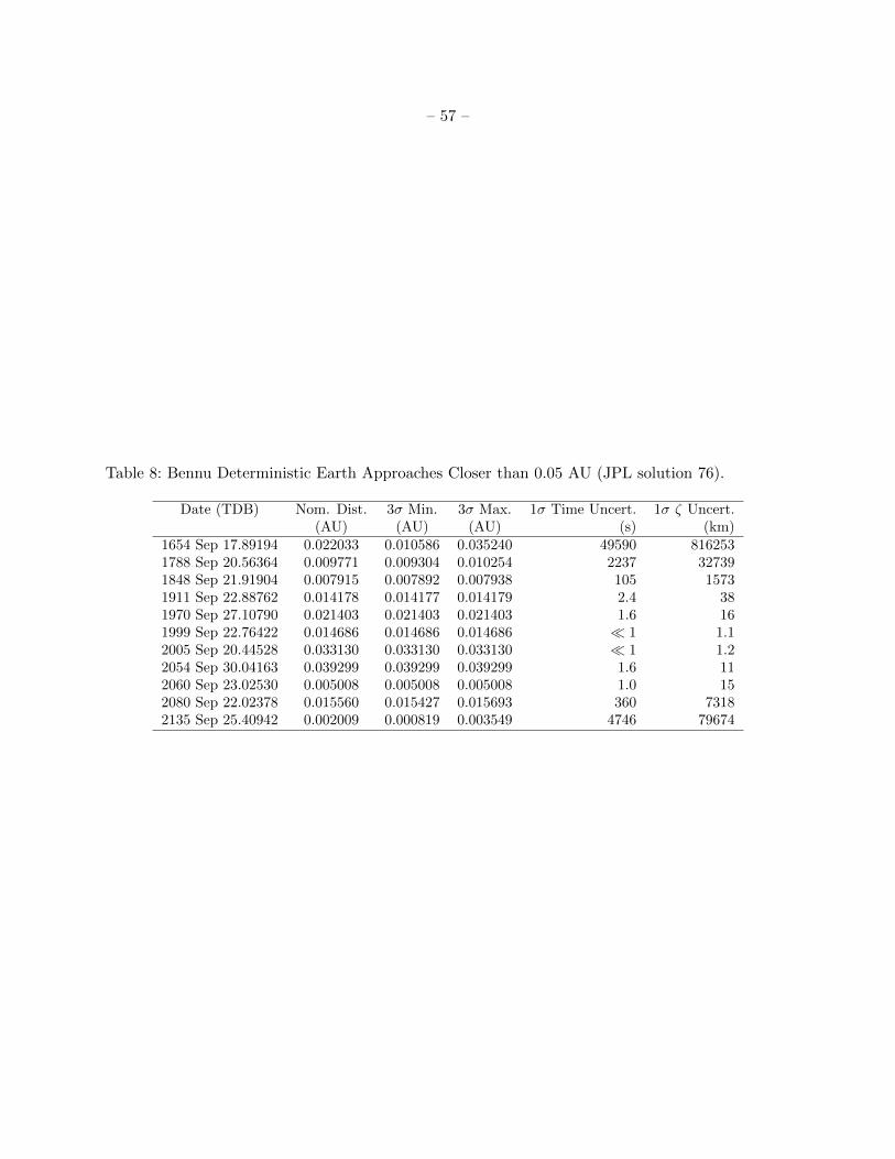
– 57 –
Table 8: Bennu Deterministic Earth Approaches Closer than 0.05 AU (JPL solution 76).
Date (TDB) Nom. Dist. 3σ Min. 3σ Max. 1σ Time Uncert. 1σ ζ Uncert.(AU) (AU) (AU) (s) (km)
1654 Sep 17.89194 0.022033 0.010586 0.035240 49590 8162531788 Sep 20.56364 0.009771 0.009304 0.010254 2237 327391848 Sep 21.91904 0.007915 0.007892 0.007938 105 15731911 Sep 22.88762 0.014178 0.014177 0.014179 2.4 381970 Sep 27.10790 0.021403 0.021403 0.021403 1.6 161999 Sep 22.76422 0.014686 0.014686 0.014686 1 1.12005 Sep 20.44528 0.033130 0.033130 0.033130 1 1.22054 Sep 30.04163 0.039299 0.039299 0.039299 1.6 112060 Sep 23.02530 0.005008 0.005008 0.005008 1.0 152080 Sep 22.02378 0.015560 0.015427 0.015693 360 73182135 Sep 25.40942 0.002009 0.000819 0.003549 4746 79674

– 58 –
Table 9: Keyholes in 2135 b-plane and associated impact probabilities, JPL solution 76.
Year ζ2135 ζ-width Impact Palermo Year ζ2135 ζ-width Impact Palermo(km) (km) Prob. Scale (km) (km) Prob. Scale
2192 92981 0.17 1.04× 10⁻¹⁰ −8.27 2195 343783 0.11 4.15× 10−07 −4.672187 93280 0.32 2.01× 10⁻¹⁰ −7.97 2181 347699 0.78 2.86× 10−06 −3.802198 99162 0.25 3.33× 10⁻¹⁰ −7.78 2175 349704 1.80 6.43× 10−06 −3.432187 105731 0.12 3.44× 10⁻¹⁰ −7.74 2186 367729 0.32 8.12× 10−07 −4.362182 105945 3.59 1.08× 10−08 −6.23 2175 368877 16.67 4.13× 10−05 −2.632197 148127 0.19 3.08× 10−08 −5.81 2181 370007 0.56 1.35× 10−06 −4.132182 153125 6.29 1.42× 10−06 −4.11 2193 391326 0.60 8.52× 10−07 −4.362187 153481 0.21 4.94× 10−08 −5.58 2187 392308 5.97 8.34× 10−06 −3.352192 161203 1.53 5.83× 10−07 −4.52 2198 393200 0.11 1.47× 10−07 −5.132193 162322 0.15 6.04× 10−08 −5.51 2181 405893 0.64 6.27× 10−07 −4.462182 171554 5.15 3.55× 10−06 −3.71 2187 429187 0.51 2.43× 10−07 −4.892187 171842 0.17 1.19× 10−07 −5.20 2181 430234 0.20 9.41× 10−08 −5.282187 174357 0.66 5.25× 10−07 −4.55 2176 449272 12.23 3.07× 10−06 −3.762192 174935 0.40 3.31× 10−07 −4.76 2193 459392 0.12 2.09× 10−08 −5.972194 177766 0.17 1.57× 10−07 −5.09 2188 475391 7.74 7.99× 10−07 −4.372199 185793 0.19 2.56× 10−07 −4.89 2194 479545 9.54 8.50× 10−07 −4.362193 186415 19.84 2.75× 10−05 −2.85 2194 486578 25.51 1.77× 10−06 −4.042198 186996 0.21 2.97× 10−07 −4.83 2194 511097 24.90 6.94× 10−07 −4.452199 191883 0.20 3.53× 10−07 −4.75 2188 517881 0.75 1.61× 10−08 −6.072198 208524 0.53 1.53× 10−06 −4.11 2193 527510 0.89 1.30× 10−08 −6.172190 211276 0.11 3.50× 10−07 −4.74 2181 528840 0.65 9.06× 10−09 −6.302199 235014 0.17 8.69× 10−07 −4.36 2193 534125 0.20 2.21× 10−09 −6.942192 272823 0.12 8.39× 10−07 −4.36 2193 534310 0.19 2.13× 10−09 −6.962198 273950 0.11 7.79× 10−07 −4.41 2198 534527 0.45 4.96× 10−09 −6.602186 274243 0.21 1.48× 10−06 −4.10 2198 536801 0.13 1.30× 10−09 −7.182191 275096 0.18 1.29× 10−06 −4.17 2198 536823 0.21 2.08× 10−09 −6.982191 275569 0.77 5.44× 10−06 −3.55 2196 537259 0.12 1.19× 10−09 −7.222191 276541 0.20 1.42× 10−06 −4.13 2189 537324 0.11 1.09× 10−09 −7.242185 278479 2.76 1.96× 10−05 −2.98 2199 539780 0.23 2.11× 10−09 −6.982196 279590 4.96 3.52× 10−05 −2.75 2185 541921 0.77 6.37× 10−09 −6.462196 281070 13.32 9.45× 10−05 −2.32 2185 542397 1.72 1.39× 10−08 −6.122185 295318 9.42 6.33× 10−05 −2.47 2185 543753 0.37 2.84× 10−09 −6.812190 302940 0.20 1.24× 10−06 −4.18 2197 545747 0.26 1.84× 10−09 −7.032180 316352 3.48 1.95× 10−05 −2.96 2190 558169 11.57 4.86× 10−08 −5.592191 316680 0.19 1.05× 10−06 −4.26 2196 561278 12.31 4.54× 10−08 −5.642186 326599 0.19 9.38× 10−07 −4.30 2196 565865 20.20 6.12× 10−08 −5.512180 339506 2.73 1.14× 10−05 −3.20 2190 618399 17.45 4.95× 10−09 −6.592191 339838 0.13 5.60× 10−07 −4.53 2184 636299 54.23 6.51× 10−09 −6.452190 343541 0.17 6.74× 10−07 −4.45 2184 651571 4.35 2.45× 10⁻¹⁰ −7.88
Note: Impact probabilities > 10−5 are highlighted in bold.

– 59 –
Table 10: Resonances associated with the eight potential impacts with impact probability > 10−5.
Year ζ2135 Post-2135 Period Resonance Res. Period ∆P(km) (yr) (yr) (yr)
2193 186415 1.2342 58 yr/47 rev 1.2340 +0.00022185 278479 1.2215 50 yr/41 rev 1.2195 +0.00202196 279590 1.2213 61 yr/50 rev 1.2200 +0.00132196 281070 1.2211 61 yr/50 rev 1.2200 +0.00112185 295318 1.2194 50 yr/41 rev 1.2195 −0.00012180 316352 1.2169 45 yr/37 rev 1.2162 +0.00072180 339506 1.2144 45 yr/37 rev 1.2162 −0.00182175 368877 1.2116 40 yr/33 rev 1.2121 −0.0005

– 60 –
Table 11: Formal uncertainties with and without simulated OSIRIS-REx pseudo-range measure-ments as described in the text.
UncertaintiesReference With sim. obs.
AT (10−16 au/d) 2.52 0.38
2020-Jan-04 Position (km)Radial 1.539 0.008Transverse 0.855 0.033Normal 2.461 0.098
2020-Jan-04 Velocity (mm/s)Radial 0.662 0.005Transverse 0.400 0.002Normal 1.388 0.029
ζ2135 (km) 58000 1000