orange data mining library documentation · orange data mining library documentation, release 3...
TRANSCRIPT

Orange Data Mining LibraryDocumentation
Release 3
Orange Data Mining
Mar 29, 2020


Contents
1 Tutorial 11.1 The Data . . . . . . . . . . . . . . . . . . . . . . . . . . . . . . . . . . . . . . . . . . . . . . . . . 1
1.1.1 Data Input . . . . . . . . . . . . . . . . . . . . . . . . . . . . . . . . . . . . . . . . . . . . 11.1.2 Saving the Data . . . . . . . . . . . . . . . . . . . . . . . . . . . . . . . . . . . . . . . . . 31.1.3 Exploration of the Data Domain . . . . . . . . . . . . . . . . . . . . . . . . . . . . . . . . 31.1.4 Data Instances . . . . . . . . . . . . . . . . . . . . . . . . . . . . . . . . . . . . . . . . . . 41.1.5 Orange Datasets and NumPy . . . . . . . . . . . . . . . . . . . . . . . . . . . . . . . . . . 51.1.6 Meta Attributes . . . . . . . . . . . . . . . . . . . . . . . . . . . . . . . . . . . . . . . . . 61.1.7 Missing Values . . . . . . . . . . . . . . . . . . . . . . . . . . . . . . . . . . . . . . . . . 71.1.8 Data Selection and Sampling . . . . . . . . . . . . . . . . . . . . . . . . . . . . . . . . . . 8
1.2 Classification . . . . . . . . . . . . . . . . . . . . . . . . . . . . . . . . . . . . . . . . . . . . . . . 91.2.1 Learners and Classifiers . . . . . . . . . . . . . . . . . . . . . . . . . . . . . . . . . . . . . 91.2.2 Probabilistic Classification . . . . . . . . . . . . . . . . . . . . . . . . . . . . . . . . . . . 101.2.3 Cross-Validation . . . . . . . . . . . . . . . . . . . . . . . . . . . . . . . . . . . . . . . . 101.2.4 Handful of Classifiers . . . . . . . . . . . . . . . . . . . . . . . . . . . . . . . . . . . . . . 11
1.3 Regression . . . . . . . . . . . . . . . . . . . . . . . . . . . . . . . . . . . . . . . . . . . . . . . . 121.3.1 Handful of Regressors . . . . . . . . . . . . . . . . . . . . . . . . . . . . . . . . . . . . . 121.3.2 Cross Validation . . . . . . . . . . . . . . . . . . . . . . . . . . . . . . . . . . . . . . . . . 13
2 Reference 152.1 Data model (data) . . . . . . . . . . . . . . . . . . . . . . . . . . . . . . . . . . . . . . . . . . . 15
2.1.1 Data Storage (storage) . . . . . . . . . . . . . . . . . . . . . . . . . . . . . . . . . . . . 162.1.2 Data Table (table) . . . . . . . . . . . . . . . . . . . . . . . . . . . . . . . . . . . . . . 182.1.3 SQL table (data.sql) . . . . . . . . . . . . . . . . . . . . . . . . . . . . . . . . . . . . 212.1.4 Domain description (domain) . . . . . . . . . . . . . . . . . . . . . . . . . . . . . . . . . 242.1.5 Variable Descriptors (variable) . . . . . . . . . . . . . . . . . . . . . . . . . . . . . . . 272.1.6 Values (value) . . . . . . . . . . . . . . . . . . . . . . . . . . . . . . . . . . . . . . . . . 342.1.7 Data Instance (instance) . . . . . . . . . . . . . . . . . . . . . . . . . . . . . . . . . . 342.1.8 Data Filters (filter) . . . . . . . . . . . . . . . . . . . . . . . . . . . . . . . . . . . . . 362.1.9 Loading and saving data (io) . . . . . . . . . . . . . . . . . . . . . . . . . . . . . . . . . 38
2.2 Data Preprocessing (preprocess) . . . . . . . . . . . . . . . . . . . . . . . . . . . . . . . . . . 412.2.1 Impute . . . . . . . . . . . . . . . . . . . . . . . . . . . . . . . . . . . . . . . . . . . . . . 412.2.2 Discretization . . . . . . . . . . . . . . . . . . . . . . . . . . . . . . . . . . . . . . . . . . 412.2.3 Continuization . . . . . . . . . . . . . . . . . . . . . . . . . . . . . . . . . . . . . . . . . 432.2.4 Normalization . . . . . . . . . . . . . . . . . . . . . . . . . . . . . . . . . . . . . . . . . . 452.2.5 Randomization . . . . . . . . . . . . . . . . . . . . . . . . . . . . . . . . . . . . . . . . . 46
i

2.2.6 Remove . . . . . . . . . . . . . . . . . . . . . . . . . . . . . . . . . . . . . . . . . . . . . 462.2.7 Feature selection . . . . . . . . . . . . . . . . . . . . . . . . . . . . . . . . . . . . . . . . 472.2.8 Preprocessors . . . . . . . . . . . . . . . . . . . . . . . . . . . . . . . . . . . . . . . . . . 50
2.3 Outlier detection (classification) . . . . . . . . . . . . . . . . . . . . . . . . . . . . . . . . . 502.3.1 One Class Support Vector Machines . . . . . . . . . . . . . . . . . . . . . . . . . . . . . . 502.3.2 Elliptic Envelope . . . . . . . . . . . . . . . . . . . . . . . . . . . . . . . . . . . . . . . . 512.3.3 Local Outlier Factor . . . . . . . . . . . . . . . . . . . . . . . . . . . . . . . . . . . . . . 512.3.4 Isolation Forest . . . . . . . . . . . . . . . . . . . . . . . . . . . . . . . . . . . . . . . . . 51
2.4 Classification (classification) . . . . . . . . . . . . . . . . . . . . . . . . . . . . . . . . . . 522.4.1 Logistic Regression . . . . . . . . . . . . . . . . . . . . . . . . . . . . . . . . . . . . . . . 522.4.2 Random Forest . . . . . . . . . . . . . . . . . . . . . . . . . . . . . . . . . . . . . . . . . 532.4.3 Simple Random Forest . . . . . . . . . . . . . . . . . . . . . . . . . . . . . . . . . . . . . 532.4.4 Softmax Regression . . . . . . . . . . . . . . . . . . . . . . . . . . . . . . . . . . . . . . . 542.4.5 k-Nearest Neighbors . . . . . . . . . . . . . . . . . . . . . . . . . . . . . . . . . . . . . . 542.4.6 Naive Bayes . . . . . . . . . . . . . . . . . . . . . . . . . . . . . . . . . . . . . . . . . . . 542.4.7 Support Vector Machines . . . . . . . . . . . . . . . . . . . . . . . . . . . . . . . . . . . . 552.4.8 Linear Support Vector Machines . . . . . . . . . . . . . . . . . . . . . . . . . . . . . . . . 552.4.9 Nu-Support Vector Machines . . . . . . . . . . . . . . . . . . . . . . . . . . . . . . . . . . 562.4.10 Classification Tree . . . . . . . . . . . . . . . . . . . . . . . . . . . . . . . . . . . . . . . 562.4.11 Simple Tree . . . . . . . . . . . . . . . . . . . . . . . . . . . . . . . . . . . . . . . . . . . 572.4.12 Majority Classifier . . . . . . . . . . . . . . . . . . . . . . . . . . . . . . . . . . . . . . . 572.4.13 Neural Network . . . . . . . . . . . . . . . . . . . . . . . . . . . . . . . . . . . . . . . . . 582.4.14 CN2 Rule Induction . . . . . . . . . . . . . . . . . . . . . . . . . . . . . . . . . . . . . . . 582.4.15 Calibration and threshold optimization . . . . . . . . . . . . . . . . . . . . . . . . . . . . . 60
2.5 Regression (regression) . . . . . . . . . . . . . . . . . . . . . . . . . . . . . . . . . . . . . . . 612.5.1 Linear Regression . . . . . . . . . . . . . . . . . . . . . . . . . . . . . . . . . . . . . . . . 612.5.2 Polynomial . . . . . . . . . . . . . . . . . . . . . . . . . . . . . . . . . . . . . . . . . . . 632.5.3 Mean . . . . . . . . . . . . . . . . . . . . . . . . . . . . . . . . . . . . . . . . . . . . . . 632.5.4 Random Forest . . . . . . . . . . . . . . . . . . . . . . . . . . . . . . . . . . . . . . . . . 642.5.5 Simple Random Forest . . . . . . . . . . . . . . . . . . . . . . . . . . . . . . . . . . . . . 642.5.6 Regression Tree . . . . . . . . . . . . . . . . . . . . . . . . . . . . . . . . . . . . . . . . . 652.5.7 Neural Network . . . . . . . . . . . . . . . . . . . . . . . . . . . . . . . . . . . . . . . . . 66
2.6 Clustering (clustering) . . . . . . . . . . . . . . . . . . . . . . . . . . . . . . . . . . . . . . . 662.6.1 Hierarchical (hierarchical) . . . . . . . . . . . . . . . . . . . . . . . . . . . . . . . . 66
2.7 Distance (distance) . . . . . . . . . . . . . . . . . . . . . . . . . . . . . . . . . . . . . . . . . . 672.7.1 Handling discrete and missing data . . . . . . . . . . . . . . . . . . . . . . . . . . . . . . . 692.7.2 Supported distances . . . . . . . . . . . . . . . . . . . . . . . . . . . . . . . . . . . . . . . 69
2.8 Evaluation (evaluation) . . . . . . . . . . . . . . . . . . . . . . . . . . . . . . . . . . . . . . . 712.8.1 Sampling procedures for testing models (testing) . . . . . . . . . . . . . . . . . . . . . 712.8.2 Scoring methods (scoring) . . . . . . . . . . . . . . . . . . . . . . . . . . . . . . . . . . 752.8.3 Performance curves . . . . . . . . . . . . . . . . . . . . . . . . . . . . . . . . . . . . . . . 79
2.9 Projection (projection) . . . . . . . . . . . . . . . . . . . . . . . . . . . . . . . . . . . . . . . 802.9.1 PCA . . . . . . . . . . . . . . . . . . . . . . . . . . . . . . . . . . . . . . . . . . . . . . . 802.9.2 FreeViz . . . . . . . . . . . . . . . . . . . . . . . . . . . . . . . . . . . . . . . . . . . . . 822.9.3 LDA . . . . . . . . . . . . . . . . . . . . . . . . . . . . . . . . . . . . . . . . . . . . . . . 822.9.4 References . . . . . . . . . . . . . . . . . . . . . . . . . . . . . . . . . . . . . . . . . . . 83
2.10 Miscellaneous (misc) . . . . . . . . . . . . . . . . . . . . . . . . . . . . . . . . . . . . . . . . . . 832.10.1 Distance Matrix (distmatrix) . . . . . . . . . . . . . . . . . . . . . . . . . . . . . . . . 83
Bibliography 87
Python Module Index 89
Index 91
ii
CHAPTER 1
Tutorial
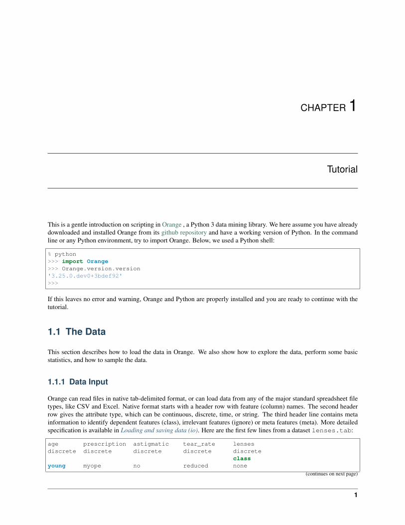
This is a gentle introduction on scripting in Orange , a Python 3 data mining library. We here assume you have alreadydownloaded and installed Orange from its github repository and have a working version of Python. In the commandline or any Python environment, try to import Orange. Below, we used a Python shell:
% python>>> import Orange>>> Orange.version.version'3.25.0.dev0+3bdef92'>>>
If this leaves no error and warning, Orange and Python are properly installed and you are ready to continue with thetutorial.
1.1 The Data
This section describes how to load the data in Orange. We also show how to explore the data, perform some basicstatistics, and how to sample the data.
1.1.1 Data Input
Orange can read files in native tab-delimited format, or can load data from any of the major standard spreadsheet filetypes, like CSV and Excel. Native format starts with a header row with feature (column) names. The second headerrow gives the attribute type, which can be continuous, discrete, time, or string. The third header line contains metainformation to identify dependent features (class), irrelevant features (ignore) or meta features (meta). More detailedspecification is available in Loading and saving data (io). Here are the first few lines from a dataset lenses.tab:
age prescription astigmatic tear_rate lensesdiscrete discrete discrete discrete discrete
classyoung myope no reduced none
(continues on next page)
1
Orange Data Mining Library Documentation, Release 3
(continued from previous page)
young myope no normal softyoung myope yes reduced noneyoung myope yes normal hardyoung hypermetrope no reduced none
Values are tab-limited. This dataset has four attributes (age of the patient, spectacle prescription, notion on astig-matism, and information on tear production rate) and an associated three-valued dependent variable encoding lensprescription for the patient (hard contact lenses, soft contact lenses, no lenses). Feature descriptions could use oneletter only, so the header of this dataset could also read:
age prescription astigmatic tear_rate lensesd d d d d
c
The rest of the table gives the data. Note that there are 5 instances in our table above. For the full dataset, check outor download lenses.tab) to a target directory. You can also skip this step as Orange comes preloaded with severaldemo datasets, lenses being one of them. Now, open a python shell, import Orange and load the data:
>>> import Orange>>> data = Orange.data.Table("lenses")>>>
Note that for the file name no suffix is needed, as Orange checks if any files in the current directory are of a readabletype. The call to Orange.data.Table creates an object called data that holds your dataset and information aboutthe lenses domain:
>>> data.domain.attributes(DiscreteVariable('age', values=('pre-presbyopic', 'presbyopic', 'young')),DiscreteVariable('prescription', values=('hypermetrope', 'myope')),DiscreteVariable('astigmatic', values=('no', 'yes')),DiscreteVariable('tear_rate', values=('normal', 'reduced')))
>>> data.domain.class_varDiscreteVariable('lenses', values=('hard', 'none', 'soft'))>>> for d in data[:3]:
...: print(d)
...:[young, myope, no, reduced | none][young, myope, no, normal | soft][young, myope, yes, reduced | none]>>>
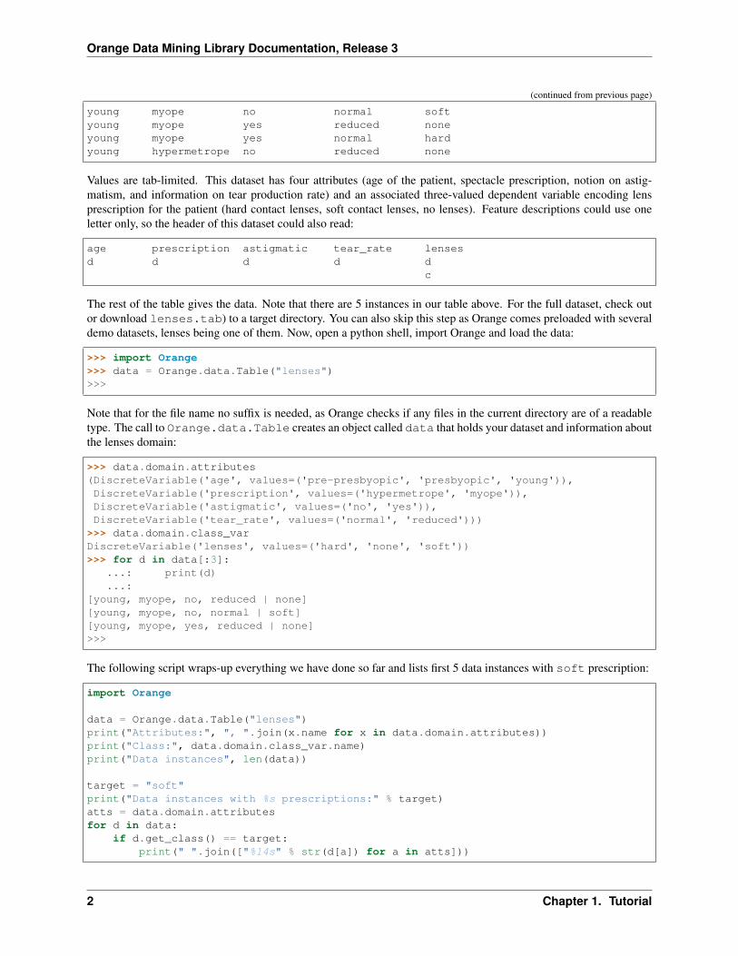
The following script wraps-up everything we have done so far and lists first 5 data instances with soft prescription:
import Orange
data = Orange.data.Table("lenses")print("Attributes:", ", ".join(x.name for x in data.domain.attributes))print("Class:", data.domain.class_var.name)print("Data instances", len(data))
target = "soft"print("Data instances with %s prescriptions:" % target)atts = data.domain.attributesfor d in data:
if d.get_class() == target:print(" ".join(["%14s" % str(d[a]) for a in atts]))
2 Chapter 1. Tutorial

Orange Data Mining Library Documentation, Release 3
Note that data is an object that holds both the data and information on the domain. We show above how to accessattribute and class names, but there is much more information there, including that on feature type, set of values forcategorical features, and other.
1.1.2 Saving the Data
Data objects can be saved to a file:
>>> data.save("new_data.tab")>>>
This time, we have to provide the file extension to specify the output format. An extension for native Orange’s dataformat is “.tab”. The following code saves only the data items with myope perscription:
import Orange
data = Orange.data.Table("lenses")myope_subset = [d for d in data if d["prescription"] == "myope"]new_data = Orange.data.Table(data.domain, myope_subset)new_data.save("lenses-subset.tab")
We have created a new data table by passing the information on the structure of the data (data.domain) and a subsetof data instances.
1.1.3 Exploration of the Data Domain
Data table stores information on data instances as well as on data domain. Domain holds the names of attributes,optional classes, their types and, and if categorical, the value names. The following code:
import Orange
data = Orange.data.Table("imports-85.tab")n = len(data.domain.attributes)n_cont = sum(1 for a in data.domain.attributes if a.is_continuous)n_disc = sum(1 for a in data.domain.attributes if a.is_discrete)print("%d attributes: %d continuous, %d discrete" % (n, n_cont, n_disc))
print("First three attributes:",", ".join(data.domain.attributes[i].name for i in range(3)),
)
print("Class:", data.domain.class_var.name)
outputs:
25 attributes: 14 continuous, 11 discreteFirst three attributes: symboling, normalized-losses, makeClass: price
Orange’s objects often behave like Python lists and dictionaries, and can be indexed or accessed through feature names:
print("First attribute:", data.domain[0].name)name = "fuel-type"
(continues on next page)
1.1. The Data 3
Orange Data Mining Library Documentation, Release 3
(continued from previous page)
print("Values of attribute '%s': %s" % (name, ", ".join(data.domain[name].values)))
The output of the above code is:
First attribute: symbolingValues of attribute 'fuel-type': diesel, gas
1.1.4 Data Instances
Data table stores data instances (or examples). These can be indexed or traversed as any Python list. Data instancescan be considered as vectors, accessed through element index, or through feature name.
import Orange
data = Orange.data.Table("iris")print("First three data instances:")for d in data[:3]:
print(d)
print("25-th data instance:")print(data[24])
name = "sepal width"print("Value of '%s' for the first instance:" % name, data[0][name])print("The 3rd value of the 25th data instance:", data[24][2])
The script above displays the following output:
First three data instances:[5.100, 3.500, 1.400, 0.200 | Iris-setosa][4.900, 3.000, 1.400, 0.200 | Iris-setosa][4.700, 3.200, 1.300, 0.200 | Iris-setosa]25-th data instance:[4.800, 3.400, 1.900, 0.200 | Iris-setosa]Value of 'sepal width' for the first instance: 3.500The 3rd value of the 25th data instance: 1.900
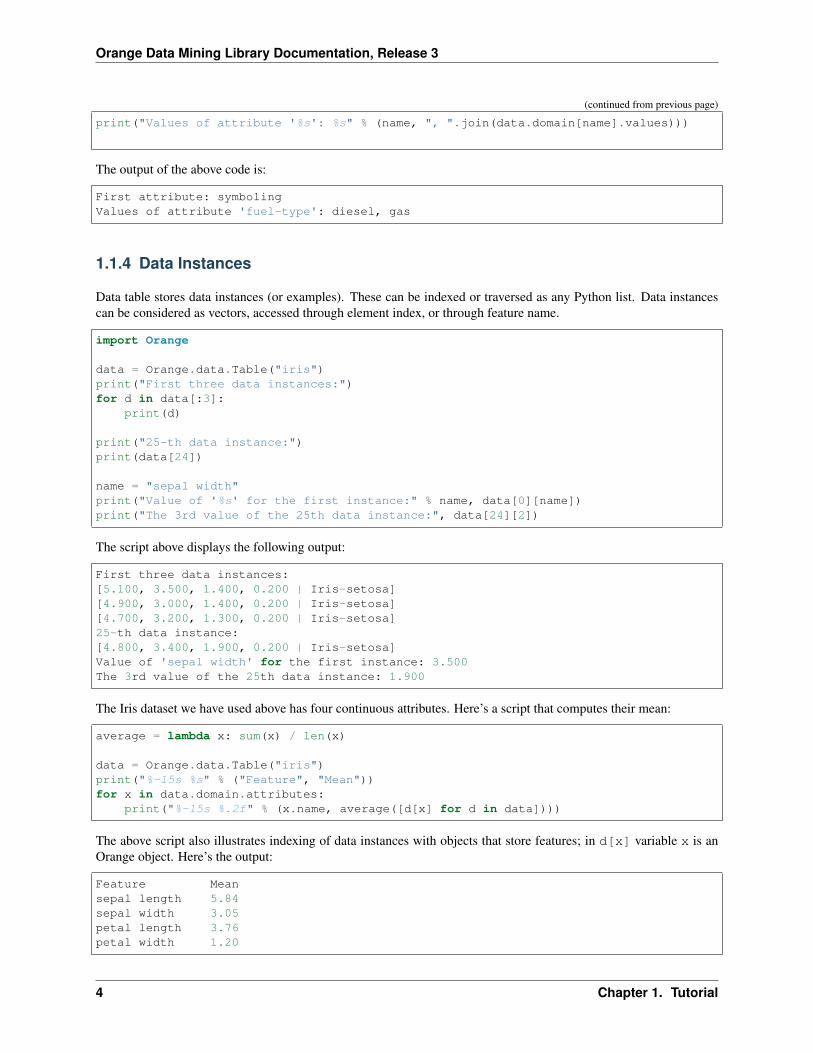
The Iris dataset we have used above has four continuous attributes. Here’s a script that computes their mean:
average = lambda x: sum(x) / len(x)
data = Orange.data.Table("iris")print("%-15s %s" % ("Feature", "Mean"))for x in data.domain.attributes:
print("%-15s %.2f" % (x.name, average([d[x] for d in data])))
The above script also illustrates indexing of data instances with objects that store features; in d[x] variable x is anOrange object. Here’s the output:
Feature Meansepal length 5.84sepal width 3.05petal length 3.76petal width 1.20
4 Chapter 1. Tutorial
Orange Data Mining Library Documentation, Release 3
A slightly more complicated, but also more interesting, code that computes per-class averages:
average = lambda xs: sum(xs) / float(len(xs))
data = Orange.data.Table("iris")targets = data.domain.class_var.valuesprint("%-15s %s" % ("Feature", " ".join("%15s" % c for c in targets)))for a in data.domain.attributes:
dist = ["%15.2f" % average([d[a] for d in data if d.get_class() == c]) for c in
→˓targets]print("%-15s" % a.name, " ".join(dist))
Of the four features, petal width and length look quite discriminative for the type of iris:
Feature Iris-setosa Iris-versicolor Iris-virginicasepal length 5.01 5.94 6.59sepal width 3.42 2.77 2.97petal length 1.46 4.26 5.55petal width 0.24 1.33 2.03
Finally, here is a quick code that computes the class distribution for another dataset:
import Orangefrom collections import Counter
data = Orange.data.Table("lenses")print(Counter(str(d.get_class()) for d in data))
1.1.5 Orange Datasets and NumPy
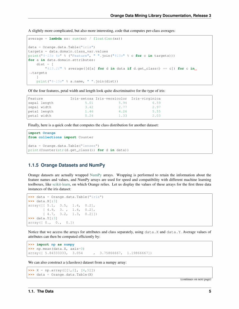
Orange datasets are actually wrapped NumPy arrays. Wrapping is performed to retain the information about thefeature names and values, and NumPy arrays are used for speed and compatibility with different machine learningtoolboxes, like scikit-learn, on which Orange relies. Let us display the values of these arrays for the first three datainstances of the iris dataset:
>>> data = Orange.data.Table("iris")>>> data.X[:3]array([[ 5.1, 3.5, 1.4, 0.2],
[ 4.9, 3. , 1.4, 0.2],[ 4.7, 3.2, 1.3, 0.2]])
>>> data.Y[:3]array([ 0., 0., 0.])
Notice that we access the arrays for attributes and class separately, using data.X and data.Y. Average values ofattributes can then be computed efficiently by:
>>> import np as numpy>>> np.mean(data.X, axis=0)array([ 5.84333333, 3.054 , 3.75866667, 1.19866667])
We can also construct a (classless) dataset from a numpy array:
>>> X = np.array([[1,2], [4,5]])>>> data = Orange.data.Table(X)
(continues on next page)
1.1. The Data 5

Orange Data Mining Library Documentation, Release 3
(continued from previous page)
>>> data.domain[Feature 1, Feature 2]
If we want to provide meaninful names to attributes, we need to construct an appropriate data domain:
>>> domain = Orange.data.Domain([Orange.data.ContinuousVariable("lenght"),Orange.data.ContinuousVariable("width")])
>>> data = Orange.data.Table(domain, X)>>> data.domain[lenght, width]
Here is another example, this time with the construction of a dataset that includes a numerical class and different typesof attributes:
size = Orange.data.DiscreteVariable("size", ["small", "big"])height = Orange.data.ContinuousVariable("height")shape = Orange.data.DiscreteVariable("shape", ["circle", "square", "oval"])speed = Orange.data.ContinuousVariable("speed")
domain = Orange.data.Domain([size, height, shape], speed)
X = np.array([[1, 3.4, 0], [0, 2.7, 2], [1, 1.4, 1]])Y = np.array([42.0, 52.2, 13.4])
data = Orange.data.Table(domain, X, Y)print(data)
Running of this scripts yields:
[[big, 3.400, circle | 42.000],[small, 2.700, oval | 52.200],[big, 1.400, square | 13.400]
1.1.6 Meta Attributes
Often, we wish to include descriptive fields in the data that will not be used in any computation (distance estimation,modeling), but will serve for identification or additional information. These are called meta attributes, and are markedwith meta in the third header row:
name hair eggs milk backbone legs typestring d d d d d dmeta classaardvark 1 0 1 1 4 mammalantelope 1 0 1 1 4 mammalbass 0 1 0 1 0 fishbear 1 0 1 1 4 mammal
Values of meta attributes and all other (non-meta) attributes are treated similarly in Orange, but stored in separatenumpy arrays:
>>> data = Orange.data.Table("zoo")>>> data[0]["name"]>>> data[0]["type"]>>> for d in data:
(continues on next page)
6 Chapter 1. Tutorial

Orange Data Mining Library Documentation, Release 3
(continued from previous page)
...: print("{}/{}: {}".format(d["name"], d["type"], d["legs"]))
...:aardvark/mammal: 4antelope/mammal: 4bass/fish: 0bear/mammal: 4>>> data.Xarray([[ 1., 0., 1., 1., 2.],
[ 1., 0., 1., 1., 2.],[ 0., 1., 0., 1., 0.],[ 1., 0., 1., 1., 2.]]))
>>> data.metasarray([['aardvark'],
['antelope'],['bass'],['bear']], dtype=object))
Meta attributes may be passed to Orange.data.Table after providing arrays for attribute and class values:
from Orange.data import Table, Domainfrom Orange.data import ContinuousVariable, DiscreteVariable, StringVariableimport numpy as np
X = np.array([[2.2, 1625], [0.3, 163]])Y = np.array([0, 1])M = np.array([["houston", 10], ["ljubljana", -1]])
domain = Domain([ContinuousVariable("population"), ContinuousVariable("area")],[DiscreteVariable("snow", ("no", "yes"))],[StringVariable("city"), StringVariable("temperature")],
)data = Table(domain, X, Y, M)print(data)
The script outputs:
[[2.200, 1625.000 | no] {houston, 10},[0.300, 163.000 | yes] {ljubljana, -1}
To construct a classless domain we could pass None for the class values.
1.1.7 Missing Values
Consider the following exploration of the dataset on votes of the US senate:
>>> import numpy as np>>> data = Orange.data.Table("voting.tab")>>> data[2][?, y, y, ?, y, ... | democrat]>>> np.isnan(data[2][0])True>>> np.isnan(data[2][1])False
1.1. The Data 7
Orange Data Mining Library Documentation, Release 3
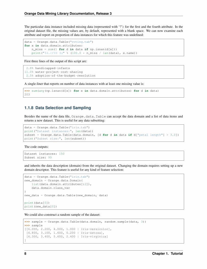
The particular data instance included missing data (represented with ‘?’) for the first and the fourth attribute. In theoriginal dataset file, the missing values are, by default, represented with a blank space. We can now examine eachattribute and report on proportion of data instances for which this feature was undefined:
data = Orange.data.Table("voting.tab")for x in data.domain.attributes:
n_miss = sum(1 for d in data if np.isnan(d[x]))print("%4.1f%% %s" % (100.0 * n_miss / len(data), x.name))
First three lines of the output of this script are:
2.8% handicapped-infants11.0% water-project-cost-sharing2.5% adoption-of-the-budget-resolution
A single-liner that reports on number of data instances with at least one missing value is:
>>> sum(any(np.isnan(d[x]) for x in data.domain.attributes) for d in data)203
1.1.8 Data Selection and Sampling
Besides the name of the data file, Orange.data.Table can accept the data domain and a list of data items andreturns a new dataset. This is useful for any data subsetting:
data = Orange.data.Table("iris.tab")print("Dataset instances:", len(data))subset = Orange.data.Table(data.domain, [d for d in data if d["petal length"] > 3.0])print("Subset size:", len(subset))
The code outputs:
Dataset instances: 150Subset size: 99
and inherits the data description (domain) from the original dataset. Changing the domain requires setting up a newdomain descriptor. This feature is useful for any kind of feature selection:
data = Orange.data.Table("iris.tab")new_domain = Orange.data.Domain(
list(data.domain.attributes[:2]),data.domain.class_var
)new_data = Orange.data.Table(new_domain, data)
print(data[0])print(new_data[0])
We could also construct a random sample of the dataset:
>>> sample = Orange.data.Table(data.domain, random.sample(data, 3))>>> sample[[6.000, 2.200, 4.000, 1.000 | Iris-versicolor],[4.800, 3.100, 1.600, 0.200 | Iris-setosa],[6.300, 3.400, 5.600, 2.400 | Iris-virginica]
]
8 Chapter 1. Tutorial

Orange Data Mining Library Documentation, Release 3
or randomly sample the attributes:
>>> atts = random.sample(data.domain.attributes, 2)>>> domain = Orange.data.Domain(atts, data.domain.class_var)>>> new_data = Orange.data.Table(domain, data)>>> new_data[0][5.100, 1.400 | Iris-setosa]
1.2 Classification
Much of Orange is devoted to machine learning methods for classification, or supervised data mining. These methodsrely on data with class-labeled instances, like that of senate voting. Here is a code that loads this dataset, displays thefirst data instance and shows its predicted class (republican):
>>> import Orange>>> data = Orange.data.Table("voting")>>> data[0][n, y, n, y, y, ... | republican]
Orange implements functions for construction of classification models, their evaluation and scoring. In a nutshell, hereis the code that reports on cross-validated accuracy and AUC for logistic regression and random forests:
import Orange
data = Orange.data.Table("voting")lr = Orange.classification.LogisticRegressionLearner()rf = Orange.classification.RandomForestLearner(n_estimators=100)res = Orange.evaluation.CrossValidation(data, [lr, rf], k=5)
print("Accuracy:", Orange.evaluation.scoring.CA(res))print("AUC:", Orange.evaluation.scoring.AUC(res))
It turns out that for this domain logistic regression does well:
Accuracy: [ 0.96321839 0.95632184]AUC: [ 0.96233796 0.95671252]
For supervised learning, Orange uses learners. These are objects that receive the data and return classifiers. Learnersare passed to evaluation routines, such as cross-validation above.
1.2.1 Learners and Classifiers
Classification uses two types of objects: learners and classifiers. Learners consider class-labeled data and return aclassifier. Given the first three data instances, classifiers return the indexes of predicted class:
>>> import Orange>>> data = Orange.data.Table("voting")>>> learner = Orange.classification.LogisticRegressionLearner()>>> classifier = learner(data)>>> classifier(data[:3])array([ 0., 0., 1.])
1.2. Classification 9

Orange Data Mining Library Documentation, Release 3
Above, we read the data, constructed a logistic regression learner, gave it the dataset to construct a classifier, and usedit to predict the class of the first three data instances. We also use these concepts in the following code that predictsthe classes of the selected three instances in the dataset:
learner = Orange.classification.LogisticRegressionLearner()classifier = learner(data)c_values = data.domain.class_var.valuesfor d in data[5:8]:
c = classifier(d)print("{}, originally {}".format(c_values[int(classifier(d))], d.get_class()))
The script outputs:
democrat, originally democratrepublican, originally democratrepublican, originally republican
Logistic regression has made a mistake in the second case, but otherwise predicted correctly. No wonder, since thiswas also the data it trained from. The following code counts the number of such mistakes in the entire dataset:
data = Orange.data.Table("voting")learner = Orange.classification.LogisticRegressionLearner()classifier = learner(data)x = np.sum(data.Y != classifier(data))
1.2.2 Probabilistic Classification
To find out what is the probability that the classifier assigns to, say, democrat class, we need to call the classifier withan additional parameter that specifies the classification output type.
data = Orange.data.Table("voting")learner = Orange.classification.LogisticRegressionLearner()classifier = learner(data)target_class = 1print("Probabilities for %s:" % data.domain.class_var.values[target_class])probabilities = classifier(data, 1)for p, d in zip(probabilities[5:8], data[5:8]):
print(p[target_class], d.get_class())
The output of the script also shows how badly the logistic regression missed the class in the second case:
Probabilities for democrat:0.999506847581 democrat0.201139534658 democrat0.042347504805 republican
1.2.3 Cross-Validation
Validating the accuracy of classifiers on the training data, as we did above, serves demonstration purposes only. Anyperformance measure that assesses accuracy should be estimated on the independent test set. Such is also a procedurecalled cross-validation, which averages the evaluation scores across several runs, each time considering a differenttraining and test subsets as sampled from the original dataset:
10 Chapter 1. Tutorial

Orange Data Mining Library Documentation, Release 3
data = Orange.data.Table("titanic")lr = Orange.classification.LogisticRegressionLearner()res = Orange.evaluation.CrossValidation(data, [lr], k=5)print("Accuracy: %.3f" % Orange.evaluation.scoring.CA(res)[0])print("AUC: %.3f" % Orange.evaluation.scoring.AUC(res)[0])
Cross-validation is expecting a list of learners. The performance estimators also return a list of scores, one for everylearner. There was just one learner (lr) in the script above, hence an array of length one was returned. The scriptestimates classification accuracy and area under ROC curve:
Accuracy: 0.779AUC: 0.704
1.2.4 Handful of Classifiers
Orange includes a variety of classification algorithms, most of them wrapped from scikit-learn, including:
• logistic regression (Orange.classification.LogisticRegressionLearner)
• k-nearest neighbors (Orange.classification.knn.KNNLearner)
• support vector machines (say, Orange.classification.svm.LinearSVMLearner)
• classification trees (Orange.classification.tree.SklTreeLearner)
• random forest (Orange.classification.RandomForestLearner)
Some of these are included in the code that estimates the probability of a target class on a testing data. This time,training and test datasets are disjoint:
import Orangeimport random
random.seed(42)data = Orange.data.Table("voting")test = Orange.data.Table(data.domain, random.sample(data, 5))train = Orange.data.Table(data.domain, [d for d in data if d not in test])
tree = Orange.classification.tree.TreeLearner(max_depth=3)knn = Orange.classification.knn.KNNLearner(n_neighbors=3)lr = Orange.classification.LogisticRegressionLearner(C=0.1)
learners = [tree, knn, lr]classifiers = [learner(train) for learner in learners]
target = 0print("Probabilities for %s:" % data.domain.class_var.values[target])print("original class ", " ".join("%-5s" % l.name for l in classifiers))
c_values = data.domain.class_var.valuesfor d in test:
print(("{:<15}" + " {:.3f}" * len(classifiers)).format(
c_values[int(d.get_class())], *(c(d, 1)[target] for c in classifiers))
)
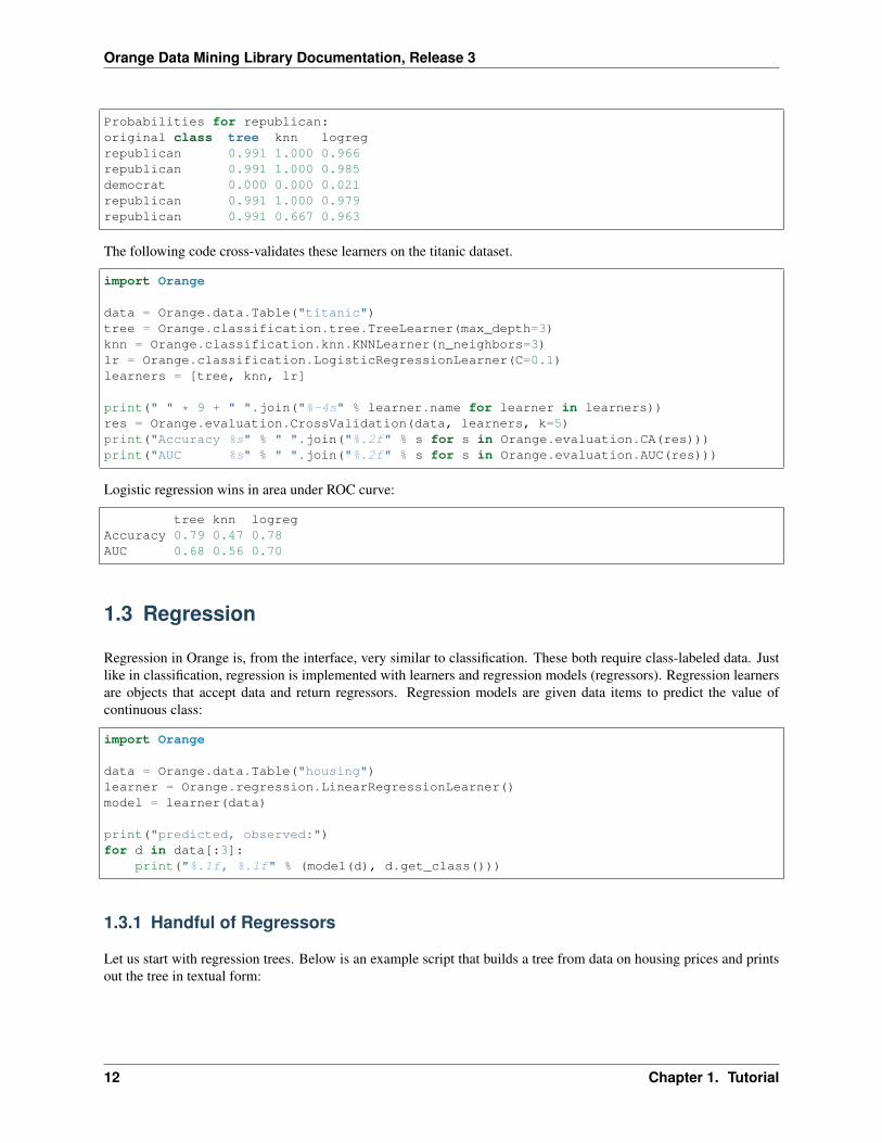
For these five data items, there are no major differences between predictions of observed classification algorithms:
1.2. Classification 11
Orange Data Mining Library Documentation, Release 3
Probabilities for republican:original class tree knn logregrepublican 0.991 1.000 0.966republican 0.991 1.000 0.985democrat 0.000 0.000 0.021republican 0.991 1.000 0.979republican 0.991 0.667 0.963
The following code cross-validates these learners on the titanic dataset.
import Orange
data = Orange.data.Table("titanic")tree = Orange.classification.tree.TreeLearner(max_depth=3)knn = Orange.classification.knn.KNNLearner(n_neighbors=3)lr = Orange.classification.LogisticRegressionLearner(C=0.1)learners = [tree, knn, lr]
print(" " * 9 + " ".join("%-4s" % learner.name for learner in learners))res = Orange.evaluation.CrossValidation(data, learners, k=5)print("Accuracy %s" % " ".join("%.2f" % s for s in Orange.evaluation.CA(res)))print("AUC %s" % " ".join("%.2f" % s for s in Orange.evaluation.AUC(res)))
Logistic regression wins in area under ROC curve:
tree knn logregAccuracy 0.79 0.47 0.78AUC 0.68 0.56 0.70
1.3 Regression
Regression in Orange is, from the interface, very similar to classification. These both require class-labeled data. Justlike in classification, regression is implemented with learners and regression models (regressors). Regression learnersare objects that accept data and return regressors. Regression models are given data items to predict the value ofcontinuous class:
import Orange
data = Orange.data.Table("housing")learner = Orange.regression.LinearRegressionLearner()model = learner(data)
print("predicted, observed:")for d in data[:3]:
print("%.1f, %.1f" % (model(d), d.get_class()))
1.3.1 Handful of Regressors
Let us start with regression trees. Below is an example script that builds a tree from data on housing prices and printsout the tree in textual form:
12 Chapter 1. Tutorial

Orange Data Mining Library Documentation, Release 3
data = Orange.data.Table("housing")tree_learner = Orange.regression.SimpleTreeLearner(max_depth=2)tree = tree_learner(data)print(tree.to_string())
The script outputs the tree:
RM<=6.941: 19.9RM>6.941| RM<=7.437| | CRIM>7.393: 14.4| | CRIM<=7.393| | | DIS<=1.886: 45.7| | | DIS>1.886: 32.7| RM>7.437| | TAX<=534.500: 45.9| | TAX>534.500: 21.9
Following is the initialization of a few other regressors and their prediction of the first five data instances in the housingprice dataset:
random.seed(42)data = Orange.data.Table("housing")test = Orange.data.Table(data.domain, random.sample(data, 5))train = Orange.data.Table(data.domain, [d for d in data if d not in test])
lin = Orange.regression.linear.LinearRegressionLearner()rf = Orange.regression.random_forest.RandomForestRegressionLearner()rf.name = "rf"ridge = Orange.regression.RidgeRegressionLearner()
learners = [lin, rf, ridge]regressors = [learner(train) for learner in learners]
print("y ", " ".join("%5s" % l.name for l in regressors))
for d in test:print(
("{:<5}" + " {:5.1f}" * len(regressors)).format(d.get_class(), *(r(d) for r in regressors)
))
Looks like the housing prices are not that hard to predict:
y linreg rf ridge22.2 19.3 21.8 19.531.6 33.2 26.5 33.221.7 20.9 17.0 21.010.2 16.9 14.3 16.814.0 13.6 14.9 13.5
1.3.2 Cross Validation
Evaluation and scoring methods are available at Orange.evaluation:
1.3. Regression 13

Orange Data Mining Library Documentation, Release 3
data = Orange.data.Table("housing.tab")
lin = Orange.regression.linear.LinearRegressionLearner()rf = Orange.regression.random_forest.RandomForestRegressionLearner()rf.name = "rf"ridge = Orange.regression.RidgeRegressionLearner()mean = Orange.regression.MeanLearner()
learners = [lin, rf, ridge, mean]
res = Orange.evaluation.CrossValidation(data, learners, k=5)rmse = Orange.evaluation.RMSE(res)r2 = Orange.evaluation.R2(res)
print("Learner RMSE R2")for i in range(len(learners)):
print("{:8s} {:.2f} {:5.2f}".format(learners[i].name, rmse[i], r2[i]))
We have scored the regression with two measures for goodness of fit: root-mean-square error and coefficient ofdetermination, or R squared. Random forest has the lowest root mean squared error:
Learner RMSE R2linreg 4.88 0.72rf 4.70 0.74ridge 4.91 0.71mean 9.20 -0.00
Not much difference here. Each regression method has a set of parameters. We have been running them with defaultparameters, and parameter fitting would help. Also, we have included MeanLearner in the list of our regressors;this regressor simply predicts the mean value from the training set, and is used as a baseline.
14 Chapter 1. Tutorial
CHAPTER 2
Reference
Available classes and methods.
2.1 Data model (data)
Orange stores data in Orange.data.Storage classes. The most commonly used storage is Orange.data.Table, which stores all data in two-dimensional numpy arrays. Each row of the data represents a data instance.
Individual data instances are represented as instances of Orange.data.Instance. Different storage classes mayderive subclasses of Instance to represent the retrieved rows in the data more efficiently and to allow modifyingthe data through modifying data instance. For example, if table is Orange.data.Table, table[0] returns the rowas Orange.data.RowInstance.
Every storage class and data instance has an associated domain description domain (an instance of Orange.data.Domain) that stores descriptions of data columns. Every column is described by an instance of aclass derived from Orange.data.Variable. The subclasses correspond to continuous variables (Orange.data.ContinuousVariable), discrete variables (Orange.data.DiscreteVariable) and string vari-ables (Orange.data.StringVariable). These descriptors contain the variable’s name, symbolic values, num-ber of decimals in printouts and similar.
The data is divided into attributes (features, independent variables), class variables (classes, targets, outcomes, depen-dent variables) and meta attributes. This division applies to domain descriptions, data storages that contain separatearrays for each of the three parts of the data and data instances.
Attributes and classes are represented with numeric values and are used in modelling. Meta attributes contain ad-ditional data which may be of any type. (Currently, only string values are supported in addition to continuous andnumeric.)
In indexing, columns can be referred to by their names, descriptors or an integer index. For example, if inst is a datainstance and var is a descriptor of type Continuous, referring to the first column in the data, which is also names“petal length”, then inst[var], inst[0] and inst[“petal length”] refer to the first value of the instance. Negative indicesare used for meta attributes, starting with -1.
Continuous and discrete values can be represented by any numerical type; by default, Orange uses double precision(64-bit) floats. Discrete values are represented by whole numbers.
15
Orange Data Mining Library Documentation, Release 3
2.1.1 Data Storage (storage)
Orange.data.storage.Storage is an abstract class representing a data object in which rows represent datainstances (examples, in machine learning terminology) and columns represent variables (features, attributes, classes,targets, meta attributes).
Data is divided into three parts that represent independent variables (X), dependent variables (Y) and meta data (metas).If practical, the class should expose those parts as properties. In the associated domain (Orange.data.Domain),the three parts correspond to lists of variable descriptors attributes, class_vars and metas.
Any of those parts may be missing, dense, sparse or sparse boolean. The difference between the later two is that thesparse data can be seen as a list of pairs (variable, value), while in the latter the variable (item) is present or absent,like in market basket analysis. The actual storage of sparse data depends upon the storage type.
There is no uniform constructor signature: every derived class provides one or more specific constructors.
There are currently two derived classes Orange.data.Table and Orange.data.sql.Table, the former stor-ing the data in-memory, in numpy objects, and the latter in SQL (currently, only PostreSQL is supported).
Derived classes must implement at least the methods for getting rows and the number of instances (__getitem__and __len__). To make storage fast enough to be practically useful, it must also reimplement a number of filters,preprocessors and aggregators. For instance, method _filter_values(self, filter) returns a new storage which onlycontains the rows that match the criteria given in the filter. Orange.data.Table implements an efficient methodbased on numpy indexing, and Orange.data.sql.Table, which “stores” a table as an SQL query, converts thefilter into a WHERE clause.
Orange.data.storage.domain(:obj:‘Orange.data.Domain‘)The domain describing the columns of the data
Data access
Orange.data.storage.__getitem__(self, index)Return one or more rows of the data.
• If the index is an int, e.g. data[7]; the corresponding row is returned as an instance of Instance.Concrete implementations of Storage use specific derived classes for instances.
• If the index is a slice or a sequence of ints (e.g. data[7:10] or data[[7, 42, 15]], indexing returns a newstorage with the selected rows.
• If there are two indices, where the first is an int (a row number) and the second can be interpreted ascolumns, e.g. data[3, 5] or data[3, ‘gender’] or data[3, y] (where y is an instance of Variable), a singlevalue is returned as an instance of Value.
• In all other cases, the first index should be a row index, a slice or a sequence, and the second index, whichrepresent a set of columns, should be an int, a slice, a sequence or a numpy array. The result is a newstorage with a new domain.
.__len__(self)Return the number of data instances (rows)
Inspection
Storage.X_density, Storage.Y_density, Storage.metas_densityIndicates whether the attributes, classes and meta attributes are dense (Storage.DENSE) or sparse (Stor-age.SPARSE). If they are sparse and all values are 0 or 1, it is marked as (Storage.SPARSE_BOOL). The Storageclass provides a default DENSE. If the data has no attibutes, classes or meta attributes, the corresponding methodshould re
16 Chapter 2. Reference

Orange Data Mining Library Documentation, Release 3
Filters
Storage should define the following methods to optimize the filtering operations as allowed by the underlying datastructure. Orange.data.Table executes them directly through numpy (or bottleneck or related) methods, whileOrange.data.sql.Table appends them to the WHERE clause of the query that defines the data.
These methods should not be called directly but through the classes defined in Orange.data.filter. Methodsin Orange.data.filter also provide the slower fallback functions for the functions not defined in the storage.
Orange.data.storage._filter_is_defined(self, columns=None, negate=False)Extract rows without undefined values.
Parameters
• columns (sequence of ints, variable names or descriptors) – op-tional list of columns that are checked for unknowns
• negate (bool) – invert the selection
Returns a new storage of the same type or Table
Return type Orange.data.storage.Storage
Orange.data.storage._filter_has_class(self, negate=False)Return rows with known value of the target attribute. If there are multiple classes, all must be defined.
Parameters negate (bool) – invert the selection
Returns a new storage of the same type or Table
Return type Orange.data.storage.Storage
Orange.data.storage._filter_same_value(self, column, value, negate=False)Select rows based on a value of the given variable.
Parameters
• column (int, str or Orange.data.Variable) – the column that is checked
• value (int, float or str) – the value of the variable
• negate (bool) – invert the selection
Returns a new storage of the same type or Table
Return type Orange.data.storage.Storage
Orange.data.storage._filter_values(self, filter)Apply a the given filter to the data.
Parameters filter (Orange.data.Filter) – A filter for selecting the rows
Returns a new storage of the same type or Table
Return type Orange.data.storage.Storage
Aggregators
Similarly to filters, storage classes should provide several methods for fast computation of statistics. These methodsare not called directly but by modules within Orange.statistics.
_compute_basic_stats(self, columns=None, include_metas=False, compute_variance=False)
Compute basic statistics for the specified variables: minimal and maximal value, the mean and a varianca (or azero placeholder), the number of missing and defined values.
2.1. Data model (data) 17

Orange Data Mining Library Documentation, Release 3
Parameters
• columns (list of ints, variable names or descriptors of type Orange.data.Variable)– a list of columns for which the statistics is computed; if None, the function computes thedata for all variables
• include_metas (bool) – a flag which tells whether to include meta attributes (applica-ble only if columns is None)
• compute_variance (bool) – a flag which tells whether to compute the variance
Returns a list with tuple (min, max, mean, variance, #nans, #non-nans) for each variable
Return type list
Orange.data.storage._compute_distributions(self, columns=None)Compute the distribution for the specified variables. The result is a list of pairs containing the distribution andthe number of rows for which the variable value was missing.
For discrete variables, the distribution is represented as a vector with absolute frequency of each value. Forcontinuous variables, the result is a 2-d array of shape (2, number-of-distinct-values); the first row contains(distinct) values of the variables and the second has their absolute frequencies.
Parameters columns (list of ints, variable names or descriptors of type Orange.data.Variable) – a list of columns for which the distributions are computed; if None, the functionruns over all variables
Returns a list of distributions
Return type list of numpy arrays
Storage._compute_contingency(col_vars=None, row_var=None)Compute contingency matrices for one or more discrete or continuous variables against the specified discretevariable.
The resulting list contains a pair for each column variable. The first element contains the contingencies andthe second elements gives the distribution of the row variables for instances in which the value of the columnvariable is missing.
The format of contingencies returned depends on the variable type:
• for discrete variables, it is a numpy array, where element (i, j) contains count of rows with i-th value of therow variable and j-th value of the column variable.
• for continuous variables, contingency is a list of two arrays, where the first array contains ordered distinctvalues of the column_variable and the element (i,j) of the second array contains count of rows with i-thvalue of the row variable and j-th value of the ordered column variable.
Parameters
• col_vars (list of ints, variable names or descriptors of type Orange.data.Variable) – variables whose values will correspond to columns of contingency matrices
• row_var (int, variable name or Orange.data.DiscreteVariable) – a discretevariable whose values will correspond to the rows of contingency matrices
2.1.2 Data Table (table)
class Orange.data.Table(*args, **kwargs)Stores data instances as a set of 2d tables representing the independent variables (attributes, features) and de-pendent variables (classes, targets), and the corresponding weights and meta attributes.
18 Chapter 2. Reference

Orange Data Mining Library Documentation, Release 3
The data is stored in 2d numpy arrays X, Y, W, metas. The arrays may be dense or sparse. All arrays have thesame number of rows. If certain data is missing, the corresponding array has zero columns.
Arrays can be of any type; default is float (that is, double precision). Values of discrete variables are stored aswhole numbers. Arrays for meta attributes usually contain instances of object.
The table also stores the associated information about the variables as an instance of Domain. The number ofcolumns must match the corresponding number of variables in the description.
There are multiple ways to get values or entire rows of the table.
• The index can be an int, e.g. table[7]; the corresponding row is returned as an instance of RowInstance.
• The index can be a slice or a sequence of ints (e.g. table[7:10] or table[[7, 42, 15]], indexing returns anew data table with the selected rows.
• If there are two indices, where the first is an int (a row number) and the second can be interpreted ascolumns, e.g. table[3, 5] or table[3, ‘gender’] or table[3, y] (where y is an instance of Variable), asingle value is returned as an instance of Value.
• In all other cases, the first index should be a row index, a slice or a sequence, and the second index, whichrepresent a set of columns, should be an int, a slice, a sequence or a numpy array. The result is a new tablewith a new domain.
Rules for setting the data are as follows.
• If there is a single index (an int, slice, or a sequence of row indices) and the value being set is a singlescalar, all attributes (not including the classes) are set to that value. That is, table[r] = v is equivalent totable.X[r] = v.
• If there is a single index and the value is a data instance (Orange.data.Instance), it is convertedinto the table’s domain and set to the corresponding rows.
• Final option for a single index is that the value is a sequence whose length equals the number of attributesand target variables. The corresponding rows are set; meta attributes are set to unknowns.
• For two indices, the row can again be given as a single int, a slice or a sequence of indices. Columnindices can be a single int, str or Orange.data.Variable, a sequence of them, a slice or anyiterable. The value can be a single value, or a sequence of appropriate length.
domainDescription of the variables corresponding to the table’s columns. The domain is used for determining thevariable types, printing the data in human-readable form, conversions between data tables and similar.
columnsA class whose attributes contain attribute descriptors for columns. For a table table, setting c = ta-ble.columns will allow accessing the table’s variables with, for instance c.gender, c.age ets. Spaces arereplaced with underscores.
Constructors
The preferred way to construct a table is to invoke a named constructor.
classmethod Table.from_domain(domain, n_rows=0, weights=False)Construct a new Table with the given number of rows for the given domain. The optional vector of weights isinitialized to 1’s.
Parameters
• domain (Orange.data.Domain) – domain for the Table
• n_rows (int) – number of rows in the new table
2.1. Data model (data) 19

Orange Data Mining Library Documentation, Release 3
• weights (bool) – indicates whether to construct a vector of weights
Returns a new table
Return type Orange.data.Table
classmethod Table.from_table(domain, source, row_indices=Ellipsis)Create a new table from selected columns and/or rows of an existing one. The columns are chosen using adomain. The domain may also include variables that do not appear in the source table; they are computed fromsource variables if possible.
The resulting data may be a view or a copy of the existing data.
Parameters
• domain (Orange.data.Domain) – the domain for the new table
• source (Orange.data.Table) – the source table
• row_indices (a slice or a sequence) – indices of the rows to include
Returns a new table
Return type Orange.data.Table
classmethod Table.from_table_rows(source, row_indices)Construct a new table by selecting rows from the source table.
Parameters
• source (Orange.data.Table) – an existing table
• row_indices (a slice or a sequence) – indices of the rows to include
Returns a new table
Return type Orange.data.Table
classmethod Table.from_numpy(domain, X, Y=None, metas=None, W=None, attributes=None,ids=None)
Construct a table from numpy arrays with the given domain. The number of variables in the domain must matchthe number of columns in the corresponding arrays. All arrays must have the same number of rows. Arrays maybe of different numpy types, and may be dense or sparse.
Parameters
• domain (Orange.data.Domain) – the domain for the new table
• X (np.array) – array with attribute values
• Y (np.array) – array with class values
• metas (np.array) – array with meta attributes
• W (np.array) – array with weights
Returns
classmethod Table.from_file(filename, sheet=None)Read a data table from a file. The path can be absolute or relative.
Parameters
• filename (str) – File name
• sheet (str) – Sheet in a file (optional)
Returns a new data table
20 Chapter 2. Reference

Orange Data Mining Library Documentation, Release 3
Return type Orange.data.Table
Inspection
Table.is_view()Return True if all arrays represent a view referring to another table
Table.is_copy()Return True if the table owns its data
Table.ensure_copy()Ensure that the table owns its data; copy arrays when necessary.
Table.has_missing()Return True if there are any missing attribute or class values.
Table.has_missing_class()Return True if there are any missing class values.
Table.checksum(include_metas=True)Return a checksum over X, Y, metas and W.
Row manipulation
Note: Methods that change the table length (append, extend, insert, clear, and resizing through deleting, slicing orby other means), were deprecated and removed in Orange 3.24.
Table.shuffle()Randomly shuffle the rows of the table.
Weights
Table.has_weights()Return True if the data instances are weighed.
Table.set_weights(weight=1)Set weights of data instances; create a vector of weights if necessary.
Table.total_weight()Return the total weight of instances in the table, or their number if they are unweighted.
2.1.3 SQL table (data.sql)
class Orange.data.sql.table.SqlTable(connection_params, table_or_sql, backend=None,type_hints=None, inspect_values=False)
SqlTable represents a table with the data which is stored in the database. Besides the inherited attributes, theobject stores a connection to the database and row filters.
Constructor connects to the database, infers the variable types from the types of the columns in the database andconstructs the corresponding domain description. Discrete and continuous variables are put among attributes,and string variables are meta attributes. The domain does not have a class.
2.1. Data model (data) 21

Orange Data Mining Library Documentation, Release 3
SqlTable overloads the data access methods for random access to rows and for iteration (__getitem__ and__iter__). It also provides methods for fast computation of basic statistics, distributions and contingency matri-ces, as well as for filtering the data. Filtering the data returns a new instance of SqlTable. The new instanceshowever differs only in that an additional filter is added to the row_filter.
All evaluation is lazy in the sense that most operations just modify the domain and the list of filters. These areused to construct an SQL query when the data is actually needed, for instance to retrieve a data row or computea distribution of values for a certain column.
connectionThe object that holds the database connection. An instance of a class compatible with Python DB API 2.0.
hostThe host name of the database server
databaseThe name of the database
table_nameThe name of the table in the database
row_filtersA list of filters that are applied when constructing the query. The filters in the should have a methodto_sql. Module Orange.data.sql.filter contains classes derived from filters in Orange.data.filter with the appropriate implementation of the method.
static __new__(cls, *args, **kwargs)Create and return a new object. See help(type) for accurate signature.
__init__(connection_params, table_or_sql, backend=None, type_hints=None, in-spect_values=False)
Create a new proxy for sql table.
To create a new SqlTable, specify the connection parameters for psycopg2 and the name of the table/sqlquery used to fetch the data.
table = SqlTable(‘database_name’, ‘table_name’) table = SqlTable(‘database_name’, ‘SELECT* FROM table’)
For complex configurations, dictionary of connection parameters can be used instead of the databasename. For documentation about connection parameters, see: http://www.postgresql.org/docs/current/static/libpq-connect.html#LIBPQ-PARAMKEYWORDS
Data domain is inferred from the columns of the table/query.
The (very quick) default setting is to treat all numeric columns as continuous variables and everything elseas strings and placed among meta attributes.
If inspect_values parameter is set to True, all column values are inspected and int/string columns with lessthan 21 values are intepreted as discrete features.
Domains can be constructed by the caller and passed in type_hints parameter. Variables from the domainare used for the columns with the matching names; for columns without the matching name in the domain,types are inferred as described above.
__getitem__(key)Indexing of SqlTable is performed in the following way:
If a single row is requested, it is fetched from the database and returned as a SqlRowInstance.
A new SqlTable with appropriate filters is constructed and returned otherwise.
22 Chapter 2. Reference
Orange Data Mining Library Documentation, Release 3
__iter__()Iterating through the rows executes the query using a cursor and then yields resulting rows as SqlRowIn-stances as they are requested.
copy()Return a copy of the SqlTable
__bool__()Return True if the SqlTable is not empty.
__len__()Return number of rows in the table. The value is cached so it is computed only the first time the length isrequested.
download_data(limit=None, partial=False)Download SQL data and store it in memory as numpy matrices.
XNumpy array with attribute values.
YNumpy array with class values.
metasNumpy array with class values.
WNumpy array with class values.
idsNumpy array with class values.
has_weights()Return True if the data instances are weighed.
classmethod from_table(domain, source, row_indices=Ellipsis)Create a new table from selected columns and/or rows of an existing one. The columns are chosen using adomain. The domain may also include variables that do not appear in the source table; they are computedfrom source variables if possible.
The resulting data may be a view or a copy of the existing data.
Parameters
• domain (Orange.data.Domain) – the domain for the new table
• source (Orange.data.Table) – the source table
• row_indices (a slice or a sequence) – indices of the rows to include
Returns a new table
Return type Orange.data.Table
checksum(include_metas=True)Return a checksum over X, Y, metas and W.
class Orange.data.sql.table.SqlRowInstance(domain, data=None)Extends Orange.data.Instance to correctly handle values of meta attributes.
2.1. Data model (data) 23

Orange Data Mining Library Documentation, Release 3
2.1.4 Domain description (domain)
Description of a domain stores a list of features, class(es) and meta attribute descriptors. A domain descriptor isattached to all tables in Orange to assign names and types to the corresponding columns. Columns in the Orange.data.Table have the roles of attributes (features, independent variables), class(es) (targets, outcomes, dependentvariables) and meta attributes; in parallel to that, the domain descriptor stores their corresponding descriptions incollections of variable descriptors of type Orange.data.Variable.
Domain descriptors are also stored in predictive models and other objects to facilitate automated conversions betweendomains, as described below.
Domains are most often constructed automatically when loading the data or wrapping the numpy arrays into Orange’sTable.
>>> from Orange.data import Table>>> iris = Table("iris")>>> iris.domain[sepal length, sepal width, petal length, petal width | iris]
class Orange.data.Domain(attributes, class_vars=None, metas=None, source=None)
attributesA tuple of descriptors (instances of Orange.data.Variable) for attributes (features, independentvariables).
>>> iris.domain.attributes(ContinuousVariable('sepal length'), ContinuousVariable('sepal width'),ContinuousVariable('petal length'), ContinuousVariable('petal width'))
class_varClass variable if the domain has a single class; None otherwise.
>>> iris.domain.class_varDiscreteVariable('iris')
class_varsA tuple of descriptors for class attributes (outcomes, dependent variables).
>>> iris.domain.class_vars(DiscreteVariable('iris'),)
variablesA list of attributes and class attributes (the concatenation of the above).
>>> iris.domain.variables(ContinuousVariable('sepal length'), ContinuousVariable('sepal width'),ContinuousVariable('petal length'), ContinuousVariable('petal width'),DiscreteVariable('iris'))
metasList of meta attributes.
anonymousTrue if the domain was constructed when converting numpy array to Orange.data.Table. Suchdomains can be converted to and from other domains even if they consist of different variable descriptorsfor as long as their number and types match.
24 Chapter 2. Reference

Orange Data Mining Library Documentation, Release 3
__init__(attributes, class_vars=None, metas=None, source=None)Initialize a new domain descriptor. Arguments give the features and the class attribute(s). They can bedescribed by descriptors (instances of Variable), or by indices or names if the source domain is given.
Parameters
• attributes (list of Variable) – a list of attributes
• class_vars (Variable or list of Variable) – target variable or a list of targetvariables
• metas (list of Variable) – a list of meta attributes
• source (Orange.data.Domain) – the source domain for attributes
Returns a new domain
Return type Domain
The following script constructs a domain with a discrete feature gender and continuous feature age, and acontinuous target salary.
>>> from Orange.data import Domain, DiscreteVariable, ContinuousVariable>>> domain = Domain([DiscreteVariable.make("gender"),... ContinuousVariable.make("age")],... ContinuousVariable.make("salary"))>>> domain[gender, age | salary]
This constructs a new domain with some features from the Iris dataset and a new feature color.
>>> new_domain = Domain(["sepal length",... "petal length",... DiscreteVariable.make("color")],... iris.domain.class_var,... source=iris.domain)>>> new_domain[sepal length, petal length, color | iris]
classmethod from_numpy(X, Y=None, metas=None)Create a domain corresponding to the given numpy arrays. This method is usually invoked from Orange.data.Table.from_numpy().
All attributes are assumed to be continuous and are named “Feature <n>”. Target variables are discrete ifthe only two values are 0 and 1; otherwise they are continuous. Discrete targets are named “Class <n>” andcontinuous are named “Target <n>”. Domain is marked as anonymous, so data from any other domainof the same shape can be converted into this one and vice-versa.
Parameters
• X (numpy.ndarray) – 2-dimensional array with data
• Y (numpy.ndarray or None) – 1- of 2- dimensional data for target
• metas (numpy.ndarray or None) – meta attributes
Returns a new domain
Return type Domain
>>> import numpy as np>>> from Orange.data import Domain
(continues on next page)
2.1. Data model (data) 25
Orange Data Mining Library Documentation, Release 3
(continued from previous page)
>>> X = np.arange(20, dtype=float).reshape(5, 4)>>> Y = np.arange(5, dtype=int)>>> domain = Domain.from_numpy(X, Y)>>> domain[Feature 1, Feature 2, Feature 3, Feature 4 | Class 1]
__getitem__(idx)Return a variable descriptor from the given argument, which can be a descriptor, index or name. If var isa descriptor, the function returns this same object.
Parameters idx (int, str or Variable) – index, name or descriptor
Returns an instance of Variable described by var
Return type Variable
>>> iris.domain[1:3](ContinuousVariable('sepal width'), ContinuousVariable('petal length'))
__len__()The number of variables (features and class attributes).
__contains__(item)Return True if the item (str, int, Variable) is in the domain.
>>> "petal length" in iris.domainTrue>>> "age" in iris.domainFalse
index(var)Return the index of the given variable or meta attribute, represented with an instance of Variable, int orstr.
>>> iris.domain.index("petal length")2
has_discrete_attributes(include_class=False, include_metas=False)Return True if domain has any discrete attributes. If include_class is set, the check includes the classattribute(s). If include_metas is set, the check includes the meta attributes.
>>> iris.domain.has_discrete_attributes()False>>> iris.domain.has_discrete_attributes(include_class=True)True
has_continuous_attributes(include_class=False, include_metas=False)Return True if domain has any continuous attributes. If include_class is set, the check includes the classattribute(s). If include_metas is set, the check includes the meta attributes.
>>> iris.domain.has_continuous_attributes()True
Domain conversion
Domain descriptors also convert data instances between different domains.
26 Chapter 2. Reference

Orange Data Mining Library Documentation, Release 3
In a typical scenario, we may want to discretize some continuous data before inducing a model. Discretiz-ers (Orange.preprocess) construct a new data table with attribute descriptors (Orange.data.variable), that include the corresponding functions for conversion from continuous to discrete values.The trained model stores this domain descriptor and uses it to convert instances from the original domainto the discretized one at prediction phase.
In general, instances are converted between domains as follows.
• If the target attribute appears in the source domain, the value is copied; two attributes are consideredthe same if they have the same descriptor.
• If the target attribute descriptor defines a function for value transformation, the value is transformed.
• Otherwise, the value is marked as missing.
An exception to this rule are domains in which the anonymous flag is set. When the source or the targetdomain is anonymous, they match if they have the same number of variables and types. In this case, thedata is copied without considering the attribute descriptors.
2.1.5 Variable Descriptors (variable)
Every variable is associated with a descriptor that stores its name and other properties. Descriptors serve three mainpurposes:
• conversion of values from textual format (e.g. when reading files) to the internal representation and back (e.g.when writing files or printing out);
• identification of variables: two variables from different datasets are considered to be the same if they have thesame descriptor;
• conversion of values between domains or datasets, for instance from continuous to discrete data, using a pre-computed transformation.
Descriptors are most often constructed when loading the data from files.
>>> from Orange.data import Table>>> iris = Table("iris")
>>> iris.domain.class_varDiscreteVariable('iris')>>> iris.domain.class_var.values['Iris-setosa', 'Iris-versicolor', 'Iris-virginica']
>>> iris.domain[0]ContinuousVariable('sepal length')>>> iris.domain[0].number_of_decimals1
Some variables are derived from others. For instance, discretizing a continuous variable gives a new, discrete variable.The new variable can compute its values from the original one.
>>> from Orange.preprocess import DomainDiscretizer>>> discretizer = DomainDiscretizer()>>> d_iris = discretizer(iris)>>> d_iris[0]DiscreteVariable('D_sepal length')>>> d_iris[0].values['<5.2', '[5.2, 5.8)', '[5.8, 6.5)', '>=6.5']
See Derived variables for a detailed explanation.
2.1. Data model (data) 27

Orange Data Mining Library Documentation, Release 3
Constructors
Orange maintains lists of existing descriptors for variables. This facilitates the reuse of descriptors: if two datasetsrefer to the same variables, they should be assigned the same descriptors so that, for instance, a model trained on onedataset can make predictions for the other.
Variable descriptors are seldom constructed in user scripts. When needed, this can be done by calling the constructordirectly or by calling the class method make. The difference is that the latter returns an existing descriptor if there isone with the same name and which matches the other conditions, such as having the prescribed list of discrete valuesfor DiscreteVariable:
>>> from Orange.data import ContinuousVariable>>> age = ContinuousVariable.make("age")>>> age1 = ContinuousVariable.make("age")>>> age2 = ContinuousVariable("age")>>> age is age1True>>> age is age2False
The first line returns a new descriptor after not finding an existing desciptor for a continuous variable named “age”.The second reuses the first descriptor. The last creates a new one since the constructor is invoked directly.
The distinction does not matter in most cases, but it is important when loading the data from different files. Orangeuses the make constructor when loading data.
Base class
class Orange.data.Variable(name=”, compute_value=None, *, sparse=False)The base class for variable descriptors contains the variable’s name and some basic properties.
nameThe name of the variable.
unknown_strA set of values that represent unknowns in conversion from textual formats. Default is {“?”, “.”, “”,“NA”, “~”, None}.
compute_valueA function for computing the variable’s value when converting from another domain which does not con-tain this variable. The function will be called with a data set (Orange.data.Table) and has to return anarray of computed values for all its instances. The base class defines a static method compute_value,which returns Unknown. Non-primitive variables must redefine it to return None.
sparseA flag about sparsity of the variable. When set, the variable suggests it should be stored in a sparse matrix.
source_variableAn optional descriptor of the source variable - if any - from which this variable is derived and computedvia compute_value.
attributesA dictionary with user-defined attributes of the variable
classmethod is_primitive(var=None)True if the variable’s values are stored as floats. Non-primitive variables can appear in the data only asmeta attributes.
28 Chapter 2. Reference

Orange Data Mining Library Documentation, Release 3
static str_val(val)Return a textual representation of variable’s value val. Argument val must be a float (for primitive vari-ables) or an arbitrary Python object (for non-primitives).
Derived classes must overload the function.
to_val(s)Convert the given argument to a value of the variable. The argument can be a string, a number orNone. For primitive variables, the base class provides a method that returns Unknown if s is found inunknown_str, and raises an exception otherwise. For non-primitive variables it returns the argumentitself.
Derived classes of primitive variables must overload the function.
Parameters s (str, float or None) – value, represented as a number, string or None
Return type float or object
val_from_str_add(s)Convert the given string to a value of the variable. The method is similar to to_val except that it onlyaccepts strings and that it adds new values to the variable’s domain where applicable.
The base class method calls to_val.
Parameters s (str) – symbolic representation of the value
Return type float or object
Continuous variables
class Orange.data.ContinuousVariable(name=”, number_of_decimals=None, com-pute_value=None, *, sparse=False)
Descriptor for continuous variables.
number_of_decimalsThe number of decimals when the value is printed out (default: 3).
adjust_decimalsA flag regulating whether the number_of_decimals is being adjusted by to_val.
The value of number_of_decimals is set to 3 and adjust_decimals is set to 2. When val_from_str_add iscalled for the first time with a string as an argument, number_of_decimals is set to the number of decimals inthe string and adjust_decimals is set to 1. In the subsequent calls of to_val, the nubmer of decimals is increasedif the string argument has a larger number of decimals.
If the number_of_decimals is set manually, adjust_decimals is set to 0 to prevent changes by to_val.
classmethod make(name, *args, **kwargs)Return an existing continuous variable with the given name, or construct and return a new one.
classmethod is_primitive(var=None)True if the variable’s values are stored as floats. Non-primitive variables can appear in the data only asmeta attributes.
str_val(val)Return the value as a string with the prescribed number of decimals.
to_val(s)Convert a value, given as an instance of an arbitrary type, to a float.
val_from_str_add(s)Convert a value from a string and adjust the number of decimals if adjust_decimals is non-zero.
2.1. Data model (data) 29

Orange Data Mining Library Documentation, Release 3
Discrete variables
class Orange.data.DiscreteVariable(name=”, values=(), ordered=False, com-pute_value=None, *, sparse=False)
Descriptor for symbolic, discrete variables. Values of discrete variables are stored as floats; the numbers corre-sponds to indices in the list of values.
valuesA list of variable’s values.
orderedSome algorithms (and, in particular, visualizations) may sometime reorder the values of the variable, e.g.alphabetically. This flag hints that the given order of values is “natural” (e.g. “small”, “middle”, “large”)and should not be changed.
classmethod make(name, *args, **kwargs)Return an existing continuous variable with the given name, or construct and return a new one.
classmethod is_primitive(var=None)True if the variable’s values are stored as floats. Non-primitive variables can appear in the data only asmeta attributes.
str_val(val)Return a textual representation of the value (self.values[int(val)]) or “?” if the value is unknown.
Parameters val (float (should be whole number)) – value
Return type str
to_val(s)Convert the given argument to a value of the variable (float). If the argument is numeric, its value isreturned without checking whether it is integer and within bounds. Unknown is returned if the argument isone of the representations for unknown values. Otherwise, the argument must be a string and the methodreturns its index in values.
Parameters s – values, represented as a number, string or None
Return type float
val_from_str_add(s)Similar to to_val, except that it accepts only strings and that it adds the value to the list if it does notexist yet.
Parameters s (str) – symbolic representation of the value
Return type float
String variables
class Orange.data.StringVariable(name=”, compute_value=None, *, sparse=False)Descriptor for string variables. String variables can only appear as meta attributes.
classmethod make(name, *args, **kwargs)Return an existing continuous variable with the given name, or construct and return a new one.
classmethod is_primitive(var=None)True if the variable’s values are stored as floats. Non-primitive variables can appear in the data only asmeta attributes.
static str_val(val)Return a string representation of the value.
30 Chapter 2. Reference

Orange Data Mining Library Documentation, Release 3
to_val(s)Return the value as a string. If it is already a string, the same object is returned.
val_from_str_add(s)Return the value as a string. If it is already a string, the same object is returned.
Time variables
Time variables are continuous variables with value 0 on the Unix epoch, 1 January 1970 00:00:00.0 UTC. Positivenumbers are dates beyond this date, and negative dates before. Due to limitation of Python datetime module, onlydates in 1 A.D. or later are supported.
class Orange.data.TimeVariable(*args, have_date=0, have_time=0, **kwargs)TimeVariable is a continuous variable with Unix epoch (1970-01-01 00:00:00+0000) as the origin (0.0). Laterdates are positive real numbers (equivalent to Unix timestamp, with microseconds in the fraction part), and thedates before it map to the negative real numbers.
Unfortunately due to limitation of Python datetime, only dates with year >= 1 (A.D.) are supported.
If time is specified without a date, Unix epoch is assumed.
If time is specified wihout an UTC offset, localtime is assumed.
parse(datestr)Return datestr, a datetime provided in one of ISO 8601 formats, parsed as a real number. Value 0 marksthe Unix epoch, positive values are the dates after it, negative before.
If date is unspecified, epoch date is assumed.
If time is unspecified, 00:00:00.0 is assumed.
If timezone is unspecified, local time is assumed.
Derived variables
The compute_value mechanism is used throughout Orange to compute all preprocessing on training data andapplying the same transformations to the testing data without hassle.
Method compute_value is usually invoked behind the scenes in conversion of domains. Such conversions are aretypically implemented within the provided wrappers and cross-validation schemes.
Derived variables in Orange
Orange saves variable transformations into the domain as compute_value functions. If Orange was not usingcompute_value, we would have to manually transform the data:
>>> from Orange.data import Domain, ContinuousVariable>>> data = Orange.data.Table("iris")>>> train = data[::2] # every second row>>> test = data[1::2] # every other second instance
We will create a new data set with a single feature, “petals”, that will be a sum of petal lengths and widths:
>>> petals = ContinuousVariable("petals")>>> derived_train = train.transform(Domain([petals],... data.domain.class_vars))
(continues on next page)
2.1. Data model (data) 31

Orange Data Mining Library Documentation, Release 3
(continued from previous page)
>>> derived_train.X = train[:, "petal width"].X + \... train[:, "petal length"].X
We have set Table’s X directly. Next, we build and evaluate a classification tree:
>>> learner = Orange.classification.TreeLearner()>>> from Orange.evaluation import CrossValidation, TestOnTestData>>> res = CrossValidation(derived_train, [learner], k=5)>>> Orange.evaluation.scoring.CA(res)[0]0.88>>> res = TestOnTestData(derived_train, test, [learner])>>> Orange.evaluation.scoring.CA(res)[0]0.3333333333333333
A classification tree shows good accuracy with cross validation, but not on separate test data, because Orange cannot reconstruct the “petals” feature for test data—we would have to reconstruct it ourselves. But if we definecompute_value and therefore store the transformation in the domain, Orange could transform both training andtest data:
>>> petals = ContinuousVariable("petals",... compute_value=lambda data: data[:, "petal width"].X + \... data[:, "petal length"].X)>>> derived_train = train.transform(Domain([petals],
data.domain.class_vars))>>> res = TestOnTestData(derived_train, test, [learner])>>> Orange.evaluation.scoring.CA(res)[0]0.9733333333333334
All preprocessors in Orange use compute_value.
Example with discretization
The following example converts features to discrete:
>>> iris = Orange.data.Table("iris")>>> iris_1 = iris[::2]>>> discretizer = Orange.preprocess.DomainDiscretizer()>>> d_iris_1 = discretizer(iris_1)
A dataset is loaded and a new table with every second instance is created. On this dataset, we compute discretizeddata, which uses the same data to set proper discretization intervals.
The discretized variable “D_sepal length” stores a function that can derive continous values into discrete:
>>> d_iris_1[0]DiscreteVariable('D_sepal length')>>> d_iris_1[0].compute_value<Orange.feature.discretization.Discretizer at 0x10d5108d0>
The function is used for converting the remaining data (as automatically happens within model validation in Orange):
>>> iris_2 = iris[1::2] # previously unselected>>> d_iris_2 = iris_2.transform(d_iris_1.domain)>>> d_iris_2[0][<5.2, [2.8, 3), <1.6, <0.2 | Iris-setosa]
32 Chapter 2. Reference

Orange Data Mining Library Documentation, Release 3
The code transforms previously unused data into the discrete domain d_iris_1.domain. Behind the scenes, the valuesfor the destination domain that are not yet in the source domain (iris_2.domain) are computed with the destinationvariables’ compute_value.
Optimization for repeated computation
Some transformations share parts of computation across variables. For example, PCA uses all input features tocompute the PCA transform. If each output PCA component was implemented with ordinary compute_value,the PCA transform would be repeatedly computed for each PCA component. To avoid repeated computation, setcompute_value to a subclass of SharedComputeValue.
class Orange.data.util.SharedComputeValue(compute_shared, variable=None)A base class that separates compute_value computation for different variables into shared and specific parts.
Parameters
• compute_shared (Callable[[Orange.data.Table], object]) – A callablethat performs computation that is shared between multiple variables. Variables sharing com-putation need to set the same instance.
• variable (Orange.data.Variable) – The original variable on which this computevalue is set. Optional.
compute(data, shared_data)Given precomputed shared data, perform variable-specific part of computation and return new variablevalues. Subclasses need to implement this function.
The following example creates normalized features that divide values by row sums and then tranforms the data. In theexample the function row_sum is called only once; if we did not use SharedComputeValue, row_sum would becalled four times, once for each feature.
iris = Orange.data.Table("iris")
def row_sum(data):return data.X.sum(axis=1, keepdims=True)
class DivideWithMean(Orange.data.util.SharedComputeValue):
def __init__(self, var, fn):super().__init__(fn)self.var = var
def compute(self, data, shared_data):return data[:, self.var].X / shared_data
divided_attributes = [Orange.data.ContinuousVariable(
"Divided " + attr.name,compute_value=DivideWithMean(attr, row_sum)
) for attr in iris.domain.attributes]
divided_domain = Orange.data.Domain(divided_attributes,iris.domain.class_vars
)
divided_iris = iris.transform(divided_domain)
2.1. Data model (data) 33

Orange Data Mining Library Documentation, Release 3
2.1.6 Values (value)
class Orange.data.variable.Value(_, __=nan)The class representing a value. The class is not used to store values but only to return them in contexts in whichwe want the value to be accompanied with the descriptor, for instance to print the symbolic value of discretevariables.
The class is derived from float, with an additional attribute variable which holds the descriptor of type Orange.data.Variable. If the value continuous or discrete, it is stored as a float. Other types of values, like strings,are stored in the attribute value.
The class overloads the methods for printing out the value: variable.repr_val and variable.str_val are used toget a suitable representation of the value.
Equivalence operator is overloaded as follows:
• unknown values are equal; if one value is unknown and the other is not, they are different;
• if the value is compared with the string, the value is converted to a string using variable.str_val and thetwo strings are compared
• if the value is stored in attribute value, it is compared with the given other value
• otherwise, the inherited comparison operator for float is called.
Finally, value defines a hash, so values can be put in sets and appear as keys in dictionaries.
variable(:obj:‘Orange.data.Variable‘)Descriptor; used for printing out and for comparing with strings
valueValue; the value can be of arbitrary type and is used only for variables that are neither discrete nor contin-uous. If value is None, the derived float value is used.
2.1.7 Data Instance (instance)
Class Instance represents a data instance, typically retrieved from a Orange.data.Table or Orange.data.sql.SqlTable. The base class contains a copy of the data; modifying does not change the data in the storage fromwhich the instance was retrieved. Derived classes (e.g. Orange.data.table.RowInstance) can representviews into various data storages, therefore changing them actually changes the data.
Like data tables, every data instance is associated with a domain and its data is split into attributes, classes, metaattributes and the weight. Its constructor thus requires a domain and, optionally, data. For the following example, weborrow the domain from the Iris dataset.
>>> from Orange.data import Table, Instance>>> iris = Table("iris")>>> inst = Instance(iris.domain, [5.2, 3.8, 1.4, 0.5, "Iris-virginica"])>>> inst[5.2, 3.8, 1.4, 0.5 | Iris-virginica]>>> inst0 = Instance(iris.domain)>>> inst0[?, ?, ?, ? | ?]
The instance’s data can be retrieved through attributes x, y and metas.
>>> inst.xarray([ 5.2, 3.8, 1.4, 0.5])>>> inst.y
(continues on next page)
34 Chapter 2. Reference
Orange Data Mining Library Documentation, Release 3
(continued from previous page)
array([ 2.])>>> inst.metasarray([], dtype=object)
Other utility functions provide for easier access to the instances data.
>>> inst.get_class()Value('iris', Iris-virginica)>>> for e in inst.attributes():... print(e)...5.23.81.40.5
class Orange.data.Instance(domain, data=None, id=None)Constructor requires a domain and the data as numpy array, an existing instance from the same or anotherdomain or any Python iterable.
Domain can be omitted it the data is given as an existing data instances.
When the instance is not from the given domain, Orange converts it.
>>> from Orange.preprocess import DomainDiscretizer>>> discretizer = DomainDiscretizer()>>> d_iris = discretizer(iris)>>> d_inst = Instance(d_iris, inst)
domainThe domain describing the instance’s values.
xInstance’s attributes as a 1-dimensional numpy array whose length equals len(self.domain.attributes).
yInstance’s classes as a 1-dimensional numpy array whose length equals len(self.domain.attributes).
metasInstance’s meta attributes as a 1-dimensional numpy array whose length equals len(self.domain.attributes).
listAll instance’s values, including attributes, classes and meta attributes, as a list whose length equalslen(self.domain.attributes) + len(self.domain.class_vars) + len(self.domain.metas).
weightThe weight of the data instance. Default is 1.
attributes()Return iterator over the instance’s attributes
classes()Return iterator over the instance’s class attributes
get_class()Return the class value as an instance of Orange.data.Value. Throws an exception if there are multi-ple classes.
get_classes()Return the class value as a list of instances of Orange.data.Value.
2.1. Data model (data) 35

Orange Data Mining Library Documentation, Release 3
set_class(value)Set the instance’s class. Throws an exception if there are multiple classes.
Rows of Data Tables
class Orange.data.RowInstance(table, row_index)RowInstance is a specialization of Instance that represents a row of Orange.data.Table. RowInstanceis returned by indexing a Table.
The difference between Instance and RowInstance is that the latter represents a view into the table: changingthe RowInstance changes the data in the table:
>>> iris[42][4.4, 3.2, 1.3, 0.2 | Iris-setosa]>>> inst = iris[42]>>> inst.set_class("Iris-virginica")>>> iris[42][4.4, 3.2, 1.3, 0.2 | Iris-virginica]
Dense tables can also be modified directly through x, y and metas.
>>> inst.x[0] = 5>>> iris[42][5.0, 3.2, 1.3, 0.2 | Iris-virginica]
Sparse tables cannot be changed in this way.
weightThe weight of the data instance. Default is 1.
set_class(value)Set the instance’s class. Throws an exception if there are multiple classes.
2.1.8 Data Filters (filter)
Instances of classes derived from Filter are used for filtering the data.
When called with an individual data instance (Orange.data.Instance), they accept or reject the instance byreturning either True or False.
When called with a data storage (e.g. an instance of Orange.data.Table) they check whether the correspondingclass provides the method that implements the particular filter. If so, the method is called and the result should beof the same type as the storage; e.g., filter methods of Orange.data.Table return new instances of Orange.data.Table, and filter methods of SQL proxies return new SQL proxies.
If the class corresponding to the storage does not implement a particular filter, the fallback computes the indices of therows to be selected and returns data[indices].
class Orange.data.filter.IsDefined(columns=None, negate=False)Select the data instances with no undefined values. The check can be restricted to a subset of columns.
The filter’s behaviour may depend upon the storage implementation.
In particular, Table with sparse matrix representation will select all data instances whose values are defined,even if they are zero. However, if individual columns are checked, it will select all rows with non-zero entriesfor this columns, disregarding whether they are stored as zero or omitted.
columnsThe columns to be checked, given as a sequence of indices, names or Orange.data.Variable.
36 Chapter 2. Reference

Orange Data Mining Library Documentation, Release 3
class Orange.data.filter.HasClass(negate=False)Return all rows for which the class value is known.
Orange.data.Table implements the filter on the sparse data so that it returns all rows for which all classvalues are defined, even if they equal zero.
class Orange.data.filter.Random(prob=None, negate=False)Return a random selection of data instances.
probThe proportion (if below 1) or the probability (if 1 or above) of selected instances
class Orange.data.filter.SameValue(column, value, negate=False)Return the data instances with the given value in the specified column.
columnThe column, described by an index, a string or Orange.data.Variable.
valueThe reference value
class Orange.data.filter.Values(conditions, conjunction=True, negate=False)Select the data instances based on conjunction or disjunction of filters derived from ValueFilter that checkvalues of individual features or another (nested) Values filter.
conditionsA list of conditions, derived from ValueFilter or Values
conjunctionIf True, the filter computes a conjunction, otherwise a disjunction
negateRevert the selection
class Orange.data.filter.FilterDiscrete(column, values)Subfilter for discrete variables, which selects the instances whose value matches one of the given values.
columnThe column to which the filter applies (int, str or Orange.data.Variable).
valuesThe list (or a set) of accepted values. If None, it checks whether the value is defined.
class Orange.data.filter.FilterContinuous(position, oper, ref=None, max=None,min=None)
Subfilter for continuous variables.
columnThe column to which the filter applies (int, str or Orange.data.Variable).
refThe reference value; also aliased to min for operators Between and Outside.
maxThe upper threshold for operators Between and Outside.
operThe operator; should be FilterContinuous.Equal, NotEqual, Less, LessEqual, Greater, GreaterEqual, Be-tween, Outside or IsDefined.
Typealias of FilterContinuous
2.1. Data model (data) 37
Orange Data Mining Library Documentation, Release 3
class Orange.data.filter.FilterString(position, oper, ref=None, max=None,case_sensitive=True, **a)
Subfilter for string variables.
columnThe column to which the filter applies (int, str or Orange.data.Variable).
refThe reference value; also aliased to min for operators Between and Outside.
maxThe upper threshold for operators Between and Outside.
operThe operator; should be FilterString.Equal, NotEqual, Less, LessEqual, Greater, GreaterEqual, Between,Outside, Contains, StartsWith, EndsWith or IsDefined.
case_sensitiveTells whether the comparisons are case sensitive
Typealias of FilterString
class Orange.data.filter.FilterStringList(column, values, case_sensitive=True)Subfilter for strings variables which checks whether the value is in the given list of accepted values.
columnThe column to which the filter applies (int, str or Orange.data.Variable).
valuesThe list (or a set) of accepted values.
case_sensitiveTells whether the comparisons are case sensitive
class Orange.data.filter.FilterRegex(column, pattern, flags=0)Filter that checks whether the values match the regular expression.
2.1.9 Loading and saving data (io)
Orange.data.Table supports loading from several file formats:
• Comma-separated values (*.csv) file,
• Tab-separated values (*.tab, *.tsv) file,
• Excel spreadsheet (*.xls, *.xlsx),
• Basket file,
• Python pickle.
In addition, the text-based files (CSV, TSV) can be compressed with gzip, bzip2 or xz (e.g. *.csv.gz).
Header Format
The data in CSV, TSV, and Excel files can be described in an extended three-line header format, or a condensedsingle-line header format.
38 Chapter 2. Reference
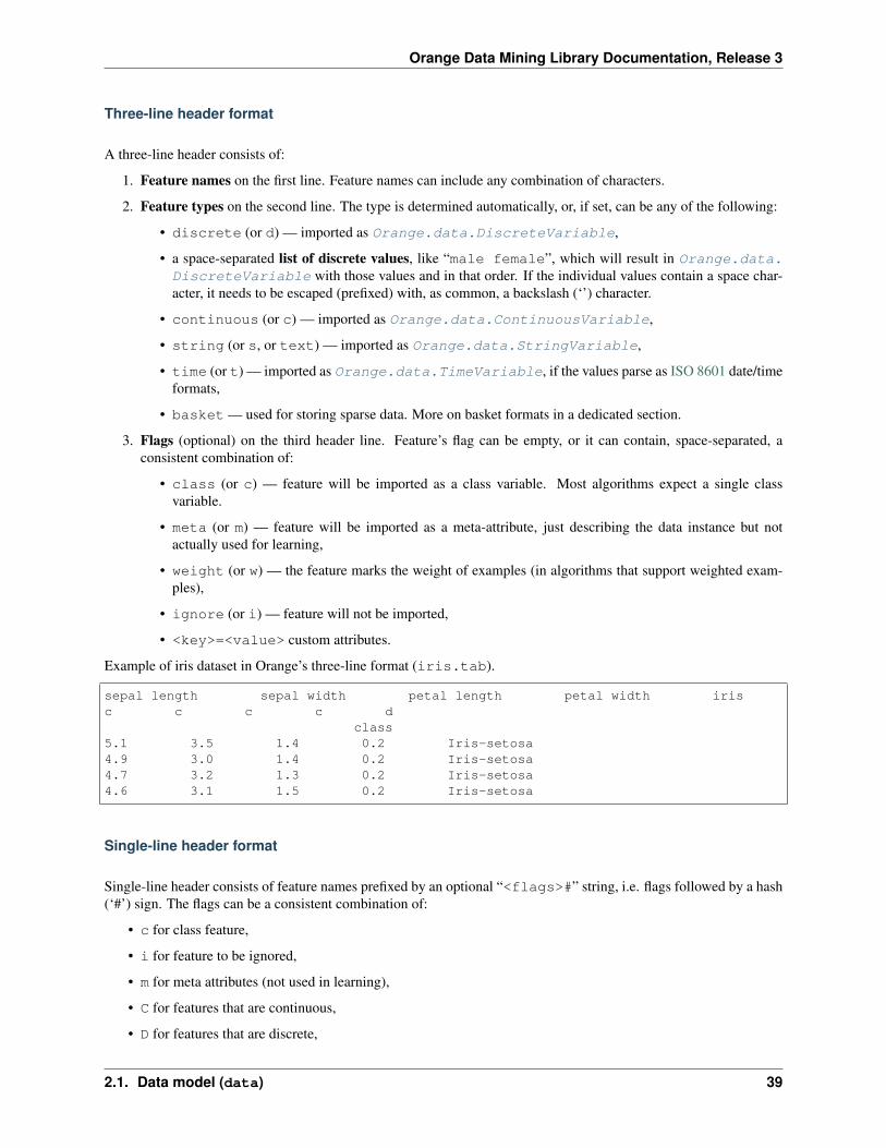
Orange Data Mining Library Documentation, Release 3
Three-line header format
A three-line header consists of:
1. Feature names on the first line. Feature names can include any combination of characters.
2. Feature types on the second line. The type is determined automatically, or, if set, can be any of the following:
• discrete (or d) — imported as Orange.data.DiscreteVariable,
• a space-separated list of discrete values, like “male female”, which will result in Orange.data.DiscreteVariable with those values and in that order. If the individual values contain a space char-acter, it needs to be escaped (prefixed) with, as common, a backslash (‘’) character.
• continuous (or c) — imported as Orange.data.ContinuousVariable,
• string (or s, or text) — imported as Orange.data.StringVariable,
• time (or t) — imported as Orange.data.TimeVariable, if the values parse as ISO 8601 date/timeformats,
• basket — used for storing sparse data. More on basket formats in a dedicated section.
3. Flags (optional) on the third header line. Feature’s flag can be empty, or it can contain, space-separated, aconsistent combination of:
• class (or c) — feature will be imported as a class variable. Most algorithms expect a single classvariable.
• meta (or m) — feature will be imported as a meta-attribute, just describing the data instance but notactually used for learning,
• weight (or w) — the feature marks the weight of examples (in algorithms that support weighted exam-ples),
• ignore (or i) — feature will not be imported,
• <key>=<value> custom attributes.
Example of iris dataset in Orange’s three-line format (iris.tab).
sepal length sepal width petal length petal width irisc c c c d
class5.1 3.5 1.4 0.2 Iris-setosa4.9 3.0 1.4 0.2 Iris-setosa4.7 3.2 1.3 0.2 Iris-setosa4.6 3.1 1.5 0.2 Iris-setosa
Single-line header format
Single-line header consists of feature names prefixed by an optional “<flags>#” string, i.e. flags followed by a hash(‘#’) sign. The flags can be a consistent combination of:
• c for class feature,
• i for feature to be ignored,
• m for meta attributes (not used in learning),
• C for features that are continuous,
• D for features that are discrete,
2.1. Data model (data) 39

Orange Data Mining Library Documentation, Release 3
• T for features that represent date and/or time in one of the ISO 8601 formats,
• S for string features.
If some (all) names or flags are omitted, the names, types, and flags are discerned automatically, and correctly (mostof the time).
Baskets
Baskets can be used for storing sparse data in tab delimited files. They were specifically designed for text miningneeds. If text mining and sparse data is not your business, you can skip this section.
Baskets are given as a list of space-separated <name>=<value> atoms. A continuous meta attribute named <name>will be created and added to the domain as optional if it is not already there. A meta value for that variable will beadded to the example. If the value is 1, you can omit the =<value> part.
It is not possible to put meta attributes of other types than continuous in the basket.
A tab delimited file with a basket can look like this:
K Ca b_foo Ba yc c basket c c
meta i class0.06 8.75 a b a c 0 10.48 b=2 d 0 10.39 7.78 0 10.57 8.22 c=13 0 1
These are the examples read from such a file:
[0.06, 1], {"Ca":8.75, "a":2.000, "b":1.000, "c":1.000}[0.48, 1], {"Ca":?, "b":2.000, "d":1.000}[0.39, 1], {"Ca":7.78}[0.57, 1], {"Ca":8.22, "c":13.000}
It is recommended to have the basket as the last column, especially if it contains a lot of data.
Note a few things. The basket column’s name, b_foo, is not used. In the first example, the value of a is 2 since itappears twice. The ordinary meta attribute, Ca, appears in all examples, even in those where its value is undefined.Meta attributes from the basket appear only where they are defined. This is due to the different nature of these metaattributes: Ca is required while the others are optional.
>>> d.domain.metas(){-6: FloatVariable 'd', -22: FloatVariable 'Ca', -5: FloatVariable 'c', -4:→˓FloatVariable 'b', -3: FloatVariable 'a'}
To fully understand all this, you should read the documentation on meta attributes in Domain and on the basket fileformat (a simple format that is limited to baskets only).
Basket Format
Basket files (.basket) are suitable for representing sparse data. Each example is represented by a line in the file. Theline is written as a comma-separated list of name-value pairs. Here’s an example of such file.
nobody, expects, the, Spanish, Inquisition=5our, chief, weapon, is, surprise=3, surprise=2, and, fear,fear, and, surprise
(continues on next page)
40 Chapter 2. Reference
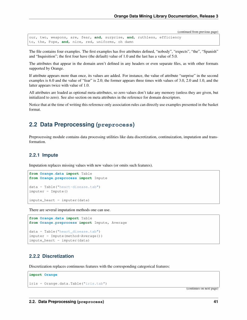
Orange Data Mining Library Documentation, Release 3
(continued from previous page)
our, two, weapons, are, fear, and, surprise, and, ruthless, efficiencyto, the, Pope, and, nice, red, uniforms, oh damn
The file contains four examples. The first examples has five attributes defined, “nobody”, “expects”, “the”, “Spanish”and “Inquisition”; the first four have (the default) value of 1.0 and the last has a value of 5.0.
The attributes that appear in the domain aren’t defined in any headers or even separate files, as with other formatssupported by Orange.
If attribute appears more than once, its values are added. For instance, the value of attribute “surprise” in the secondexamples is 6.0 and the value of “fear” is 2.0; the former appears three times with values of 3.0, 2.0 and 1.0, and thelatter appears twice with value of 1.0.
All attributes are loaded as optional meta-attributes, so zero values don’t take any memory (unless they are given, butinitialized to zero). See also section on meta attributes in the reference for domain descriptors.
Notice that at the time of writing this reference only association rules can directly use examples presented in the basketformat.
2.2 Data Preprocessing (preprocess)
Preprocessing module contains data processing utilities like data discretization, continuization, imputation and trans-formation.
2.2.1 Impute
Imputation replaces missing values with new values (or omits such features).
from Orange.data import Tablefrom Orange.preprocess import Impute
data = Table("heart-disease.tab")imputer = Impute()
impute_heart = imputer(data)
There are several imputation methods one can use.
from Orange.data import Tablefrom Orange.preprocess import Impute, Average
data = Table("heart_disease.tab")imputer = Impute(method=Average())impute_heart = imputer(data)
2.2.2 Discretization
Discretization replaces continuous features with the corresponding categorical features:
import Orange
iris = Orange.data.Table("iris.tab")
(continues on next page)
2.2. Data Preprocessing (preprocess) 41

Orange Data Mining Library Documentation, Release 3
(continued from previous page)
disc = Orange.preprocess.Discretize()disc.method = Orange.preprocess.discretize.EqualFreq(n=3)d_iris = disc(iris)
print("Original dataset:")for e in iris[:3]:
print(e)
print("Discretized dataset:")for e in d_iris[:3]:
print(e)
The variable in the new data table indicate the bins to which the original values belong.
Original dataset:[5.1, 3.5, 1.4, 0.2 | Iris-setosa][4.9, 3.0, 1.4, 0.2 | Iris-setosa][4.7, 3.2, 1.3, 0.2 | Iris-setosa]Discretized dataset:[<5.5, >=3.2, <2.5, <0.8 | Iris-setosa][<5.5, [2.8, 3.2), <2.5, <0.8 | Iris-setosa][<5.5, >=3.2, <2.5, <0.8 | Iris-setosa]
Default discretization method (four bins with approximatelly equal number of data instances) can be replaced withother methods.
iris = Orange.data.Table("iris.tab")disc = Orange.preprocess.Discretize()disc.method = Orange.preprocess.discretize.EqualFreq(n=2)
Discretization Algorithms
class Orange.preprocess.discretize.EqualWidth(n=4)Discretization into a fixed number of bins with equal widths.
nNumber of bins (default: 4).
class Orange.preprocess.discretize.EqualFreq(n=4)Discretization into bins with approximately equal number of data instances.
nNumber of bins (default: 4). The actual number may be lower if the variable has less than n distinct values.
class Orange.preprocess.discretize.EntropyMDL(force=False)Discretization into bins inferred by recursively splitting the values to minimize the class-entropy. The proce-dure stops when further splits would decrease the entropy for less than the corresponding increase of minimaldescription length (MDL). [FayyadIrani93].
If there are no suitable cut-off points, the procedure returns a single bin, which means that the new feature isconstant and can be removed.
forceInduce at least one cut-off point, even when its information gain is lower than MDL (default: False).
To add a new discretization, derive it from Discretization.
42 Chapter 2. Reference

Orange Data Mining Library Documentation, Release 3
class Orange.preprocess.discretize.DiscretizationAbstract base class for discretization classes.
2.2.3 Continuization
class Orange.preprocess.ContinuizeGiven a data table, return a new table in which the discretize attributes are replaced with continuous or removed.
• binary variables are transformed into 0.0/1.0 or -1.0/1.0 indicator variables, depending upon the argumentzero_based.
• multinomial variables are treated according to the argument multinomial_treatment.
• discrete attribute with only one possible value are removed;
import Orangetitanic = Orange.data.Table("titanic")continuizer = Orange.preprocess.Continuize()titanic1 = continuizer(titanic)
The class has a number of attributes that can be set either in constructor or, later, as attributes.
zero_basedDetermines the value used as the “low” value of the variable. When binary variables are trans-formed into continuous or when multivalued variable is transformed into multiple variables, the trans-formed variable can either have values 0.0 and 1.0 (default, zero_based=True) or -1.0 and 1.0(zero_based=False).
multinomial_treatmentDefines the treatment of multinomial variables.
Continuize.Indicators
The variable is replaced by indicator variables, each corresponding to one value of the originalvariable. For each value of the original attribute, only the corresponding new attribute will havea value of one and others will be zero. This is the default behaviour.
Note that these variables are not independent, so they cannot be used (directly) in, for instance,linear or logistic regression.
For example, dataset “titanic” has feature “status” with values “crew”, “first”, “second” and“third”, in that order. Its value for the 15th row is “first”. Continuization replaces the variablewith variables “status=crew”, “status=first”, “status=second” and “status=third”. After
continuizer = Orange.preprocess.Continuize()titanic1 = continuizer(titanic)
we have
>>> titanic.domain[status, age, sex | survived]>>> titanic1.domain[status=crew, status=first, status=second, status=third,age=adult, age=child, sex=female, sex=male | survived]
For the 15th row, the variable “status=first” has value 1 and the values of the other three variablesare 0:
2.2. Data Preprocessing (preprocess) 43
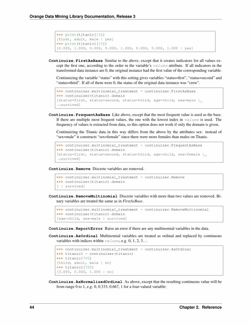
Orange Data Mining Library Documentation, Release 3
>>> print(titanic[15])[first, adult, male | yes]>>> print(titanic1[15])[0.000, 1.000, 0.000, 0.000, 1.000, 0.000, 0.000, 1.000 | yes]
Continuize.FirstAsBase Similar to the above, except that it creates indicators for all values ex-cept the first one, according to the order in the variable’s values attribute. If all indicators in thetransformed data instance are 0, the original instance had the first value of the corresponding variable.
Continuizing the variable “status” with this setting gives variables “status=first”, “status=second” and“status=third”. If all of them were 0, the status of the original data instance was “crew”.
>>> continuizer.multinomial_treatment = continuizer.FirstAsBase>>> continuizer(titanic).domain[status=first, status=second, status=third, age=child, sex=male |→˓survived]
Continuize.FrequentAsBase Like above, except that the most frequent value is used as the base.If there are multiple most frequent values, the one with the lowest index in values is used. Thefrequency of values is extracted from data, so this option does not work if only the domain is given.
Continuizing the Titanic data in this way differs from the above by the attributes sex: instead of“sex=male” it constructs “sex=female” since there were more females than males on Titanic.
>>> continuizer.multinomial_treatment = continuizer.FrequentAsBase>>> continuizer(titanic).domain[status=first, status=second, status=third, age=child, sex=female |→˓survived]
Continuize.Remove Discrete variables are removed.
>>> continuizer.multinomial_treatment = continuizer.Remove>>> continuizer(titanic).domain[ | survived]
Continuize.RemoveMultinomial Discrete variables with more than two values are removed. Bi-nary variables are treated the same as in FirstAsBase.
>>> continuizer.multinomial_treatment = continuizer.RemoveMultinomial>>> continuizer(titanic).domain[age=child, sex=male | survived]
Continuize.ReportError Raise an error if there are any multinomial variables in the data.
Continuize.AsOrdinal Multinomial variables are treated as ordinal and replaced by continuousvariables with indices within values, e.g. 0, 1, 2, 3. . .
>>> continuizer.multinomial_treatment = continuizer.AsOrdinal>>> titanic1 = continuizer(titanic)>>> titanic[700][third, adult, male | no]>>> titanic1[700][3.000, 0.000, 1.000 | no]
Continuize.AsNormalizedOrdinal As above, except that the resulting continuous value will befrom range 0 to 1, e.g. 0, 0.333, 0.667, 1 for a four-valued variable:
44 Chapter 2. Reference

Orange Data Mining Library Documentation, Release 3
>>> continuizer.multinomial_treatment = continuizer.AsNormalizedOrdinal>>> titanic1 = continuizer(titanic)>>> titanic1[700][1.000, 0.000, 1.000 | no]>>> titanic1[15][0.333, 0.000, 1.000 | yes]
transform_classIf True the class is replaced by continuous attributes or normalized as well. Multiclass problems are thustransformed to multitarget ones. (Default: False)
class Orange.preprocess.DomainContinuizerConstruct a domain in which discrete attributes are replaced by continuous.
domain_continuizer = Orange.preprocess.DomainContinuizer()domain1 = domain_continuizer(titanic)
Orange.preprocess.Continuize calls DomainContinuizer to construct the domain.
Domain continuizers can be given either a dataset or a domain, and return a new domain. When given only thedomain, use the most frequent value as the base value.
By default, the class does not change continuous and class attributes, discrete attributes are replaced with Nattributes (Indicators) with values 0 and 1.
2.2.4 Normalization
class Orange.preprocess.Normalize(zero_based=True, norm_type=Normalize.NormalizeBySD,transform_class=False, center=True, normal-ize_datetime=False)
Construct a preprocessor for normalization of features. Given a data table, preprocessor returns a new table inwhich the continuous attributes are normalized.
Parameters
• zero_based (bool (default=True)) – Only used whennorm_type=NormalizeBySpan.
Determines the value used as the “low” value of the variable. It determines the interval fornormalized continuous variables (either [-1, 1] or [0, 1]).
• norm_type (NormTypes (default: Normalize.NormalizeBySD)) – Nor-malization type. If Normalize.NormalizeBySD, the values are replaced with standardizedvalues by subtracting the average value and dividing by the standard deviation. Attributezero_based has no effect on this standardization.
If Normalize.NormalizeBySpan, the values are replaced with normalized values by subtract-ing min value of the data and dividing by span (max - min).
• transform_class (bool (default=False)) – If True the class is normalized aswell.
• center (bool (default=True)) – Only used when norm_type=NormalizeBySD.
Whether or not to center the data so it has mean zero.
• normalize_datetime (bool (default=False)) –
2.2. Data Preprocessing (preprocess) 45
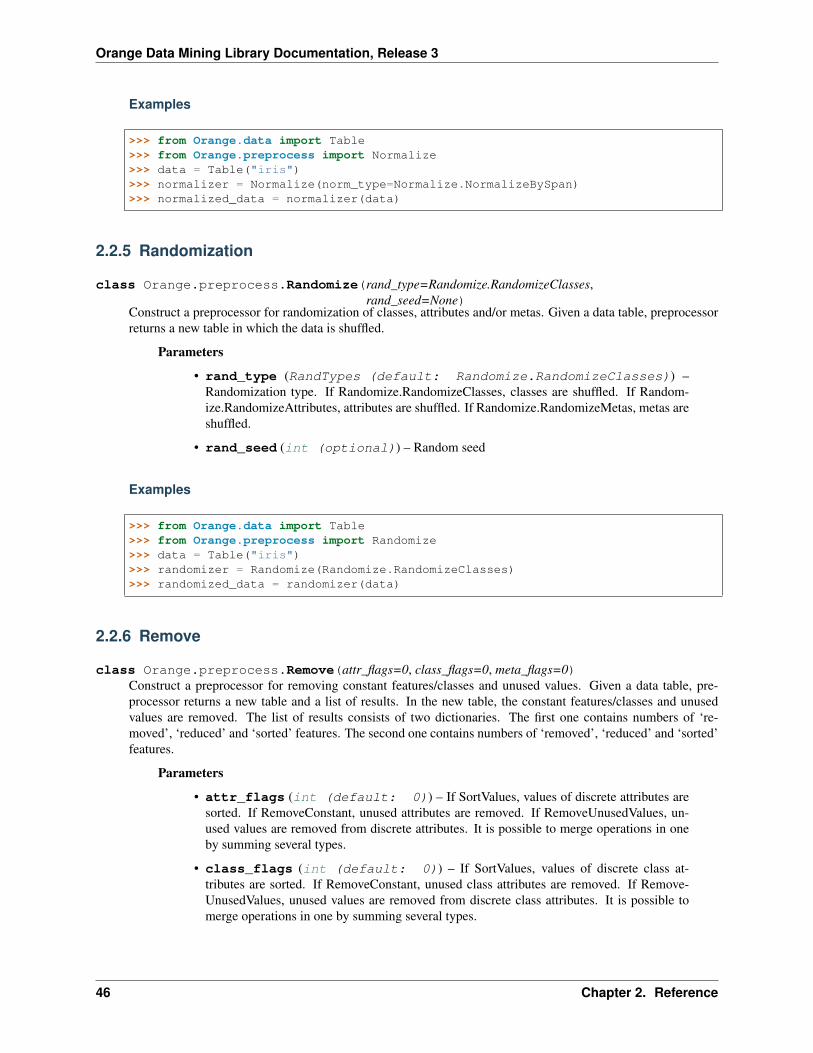
Orange Data Mining Library Documentation, Release 3
Examples
>>> from Orange.data import Table>>> from Orange.preprocess import Normalize>>> data = Table("iris")>>> normalizer = Normalize(norm_type=Normalize.NormalizeBySpan)>>> normalized_data = normalizer(data)
2.2.5 Randomization
class Orange.preprocess.Randomize(rand_type=Randomize.RandomizeClasses,rand_seed=None)
Construct a preprocessor for randomization of classes, attributes and/or metas. Given a data table, preprocessorreturns a new table in which the data is shuffled.
Parameters
• rand_type (RandTypes (default: Randomize.RandomizeClasses)) –Randomization type. If Randomize.RandomizeClasses, classes are shuffled. If Random-ize.RandomizeAttributes, attributes are shuffled. If Randomize.RandomizeMetas, metas areshuffled.
• rand_seed (int (optional)) – Random seed
Examples
>>> from Orange.data import Table>>> from Orange.preprocess import Randomize>>> data = Table("iris")>>> randomizer = Randomize(Randomize.RandomizeClasses)>>> randomized_data = randomizer(data)
2.2.6 Remove
class Orange.preprocess.Remove(attr_flags=0, class_flags=0, meta_flags=0)Construct a preprocessor for removing constant features/classes and unused values. Given a data table, pre-processor returns a new table and a list of results. In the new table, the constant features/classes and unusedvalues are removed. The list of results consists of two dictionaries. The first one contains numbers of ‘re-moved’, ‘reduced’ and ‘sorted’ features. The second one contains numbers of ‘removed’, ‘reduced’ and ‘sorted’features.
Parameters
• attr_flags (int (default: 0)) – If SortValues, values of discrete attributes aresorted. If RemoveConstant, unused attributes are removed. If RemoveUnusedValues, un-used values are removed from discrete attributes. It is possible to merge operations in oneby summing several types.
• class_flags (int (default: 0)) – If SortValues, values of discrete class at-tributes are sorted. If RemoveConstant, unused class attributes are removed. If Remove-UnusedValues, unused values are removed from discrete class attributes. It is possible tomerge operations in one by summing several types.
46 Chapter 2. Reference
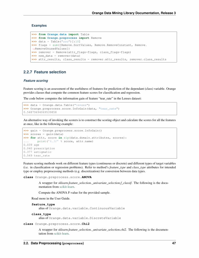
Orange Data Mining Library Documentation, Release 3
Examples
>>> from Orange.data import Table>>> from Orange.preprocess import Remove>>> data = Table("zoo")[:10]>>> flags = sum([Remove.SortValues, Remove.RemoveConstant, Remove.→˓RemoveUnusedValues])>>> remover = Remove(attr_flags=flags, class_flags=flags)>>> new_data = remover(data)>>> attr_results, class_results = remover.attr_results, remover.class_results
2.2.7 Feature selection
Feature scoring
Feature scoring is an assessment of the usefulness of features for prediction of the dependant (class) variable. Orangeprovides classes that compute the common feature scores for classification and regression.
The code below computes the information gain of feature “tear_rate” in the Lenses dataset:
>>> data = Orange.data.Table("lenses")>>> Orange.preprocess.score.InfoGain(data, "tear_rate")0.54879494069539858
An alternative way of invoking the scorers is to construct the scoring object and calculate the scores for all the featuresat once, like in the following example:
>>> gain = Orange.preprocess.score.InfoGain()>>> scores = gain(data)>>> for attr, score in zip(data.domain.attributes, scores):... print('%.3f' % score, attr.name)0.039 age0.040 prescription0.377 astigmatic0.549 tear_rate
Feature scoring methods work on different feature types (continuous or discrete) and different types of target variables(i.e. in classification or regression problems). Refer to method’s feature_type and class_type attributes for intendedtype or employ preprocessing methods (e.g. discretization) for conversion between data types.
class Orange.preprocess.score.ANOVA
A wrapper for sklearn.feature_selection._univariate_selection.f_classif. The following is the docu-mentation from scikit-learn.
Compute the ANOVA F-value for the provided sample.
Read more in the User Guide.
feature_typealias of Orange.data.variable.ContinuousVariable
class_typealias of Orange.data.variable.DiscreteVariable
class Orange.preprocess.score.Chi2
A wrapper for sklearn.feature_selection._univariate_selection.chi2. The following is the documen-tation from scikit-learn.
2.2. Data Preprocessing (preprocess) 47
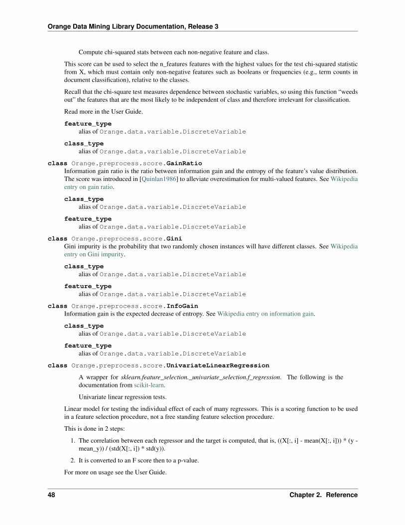
Orange Data Mining Library Documentation, Release 3
Compute chi-squared stats between each non-negative feature and class.
This score can be used to select the n_features features with the highest values for the test chi-squared statisticfrom X, which must contain only non-negative features such as booleans or frequencies (e.g., term counts indocument classification), relative to the classes.
Recall that the chi-square test measures dependence between stochastic variables, so using this function “weedsout” the features that are the most likely to be independent of class and therefore irrelevant for classification.
Read more in the User Guide.
feature_typealias of Orange.data.variable.DiscreteVariable
class_typealias of Orange.data.variable.DiscreteVariable
class Orange.preprocess.score.GainRatioInformation gain ratio is the ratio between information gain and the entropy of the feature’s value distribution.The score was introduced in [Quinlan1986] to alleviate overestimation for multi-valued features. See Wikipediaentry on gain ratio.
class_typealias of Orange.data.variable.DiscreteVariable
feature_typealias of Orange.data.variable.DiscreteVariable
class Orange.preprocess.score.GiniGini impurity is the probability that two randomly chosen instances will have different classes. See Wikipediaentry on Gini impurity.
class_typealias of Orange.data.variable.DiscreteVariable
feature_typealias of Orange.data.variable.DiscreteVariable
class Orange.preprocess.score.InfoGainInformation gain is the expected decrease of entropy. See Wikipedia entry on information gain.
class_typealias of Orange.data.variable.DiscreteVariable
feature_typealias of Orange.data.variable.DiscreteVariable
class Orange.preprocess.score.UnivariateLinearRegression
A wrapper for sklearn.feature_selection._univariate_selection.f_regression. The following is thedocumentation from scikit-learn.
Univariate linear regression tests.
Linear model for testing the individual effect of each of many regressors. This is a scoring function to be usedin a feature selection procedure, not a free standing feature selection procedure.
This is done in 2 steps:
1. The correlation between each regressor and the target is computed, that is, ((X[:, i] - mean(X[:, i])) * (y -mean_y)) / (std(X[:, i]) * std(y)).
2. It is converted to an F score then to a p-value.
For more on usage see the User Guide.
48 Chapter 2. Reference
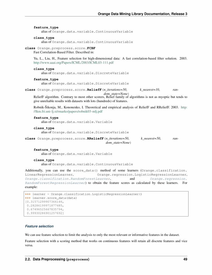
Orange Data Mining Library Documentation, Release 3
feature_typealias of Orange.data.variable.ContinuousVariable
class_typealias of Orange.data.variable.ContinuousVariable
class Orange.preprocess.score.FCBFFast Correlation-Based Filter. Described in:
Yu, L., Liu, H., Feature selection for high-dimensional data: A fast correlation-based filter solution. 2003.http://www.aaai.org/Papers/ICML/2003/ICML03-111.pdf
class_typealias of Orange.data.variable.DiscreteVariable
feature_typealias of Orange.data.variable.DiscreteVariable
class Orange.preprocess.score.ReliefF(n_iterations=50, k_nearest=10, ran-dom_state=None)
ReliefF algorithm. Contrary to most other scorers, Relief family of algorithms is not as myoptic but tends togive unreliable results with datasets with lots (hundreds) of features.
Robnik-Šikonja, M., Kononenko, I. Theoretical and empirical analysis of ReliefF and RReliefF. 2003. http://lkm.fri.uni-lj.si/rmarko/papers/robnik03-mlj.pdf
feature_typealias of Orange.data.variable.Variable
class_typealias of Orange.data.variable.DiscreteVariable
class Orange.preprocess.score.RReliefF(n_iterations=50, k_nearest=50, ran-dom_state=None)
feature_typealias of Orange.data.variable.Variable
class_typealias of Orange.data.variable.ContinuousVariable
Additionally, you can use the score_data() method of some learners (Orange.classification.LinearRegressionLearner, Orange.regression.LogisticRegressionLearner,Orange.classification.RandomForestLearner, and Orange.regression.RandomForestRegressionLearner) to obtain the feature scores as calculated by these learners. Forexample:
>>> learner = Orange.classification.LogisticRegressionLearner()>>> learner.score_data(data)[0.31571299907366146,0.28286199971877485,0.67496525667835794,0.99930286901257692]
Feature selection
We can use feature selection to limit the analysis to only the most relevant or informative features in the dataset.
Feature selection with a scoring method that works on continuous features will retain all discrete features and viceversa.
2.2. Data Preprocessing (preprocess) 49

Orange Data Mining Library Documentation, Release 3
The code below constructs a new dataset consisting of two best features according to the ANOVA method:
>>> data = Orange.data.Table("wine")>>> anova = Orange.preprocess.score.ANOVA()>>> selector = Orange.preprocess.SelectBestFeatures(method=anova, k=2)>>> data2 = selector(data)>>> data2.domain[Flavanoids, Proline | Wine]
class Orange.preprocess.SelectBestFeatures(method=None, k=None, threshold=None, de-creasing=True)
A feature selector that builds a new dataset consisting of either the top k features (if k is an int) or a proportion(if k is a float between 0.0 and 1.0), or all those that exceed a given threshold. Features are scored using theprovided feature scoring method. By default it is assumed that feature importance decreases with decreasingscores.
If both k and threshold are set, only features satisfying both conditions will be selected.
If method is not set, it is automatically selected when presented with the dataset. Datasets with both continuousand discrete features are scored using a method suitable for the majority of features.
Parameters
• method (Orange.preprocess.score.ClassificationScorer, Orange.preprocess.score.SklScorer) – Univariate feature scoring method.
• k (int or float) – The number or propotion of top features to select.
• threshold (float) – A threshold that a feature should meet according to the providedmethod.
• decreasing (boolean) – The order of feature importance when sorted from the mostto the least important feature.
2.2.8 Preprocessors
2.3 Outlier detection (classification)
2.3.1 One Class Support Vector Machines
class Orange.classification.OneClassSVMLearner(kernel=’rbf’, degree=3, gamma=’auto’,coef0=0.0, tol=0.001, nu=0.5, shrink-ing=True, cache_size=200, max_iter=-1, preprocessors=None)
A wrapper for sklearn.svm._classes.OneClassSVM. The following is its documentation:
Unsupervised Outlier Detection.
Estimate the support of a high-dimensional distribution.
The implementation is based on libsvm.
Read more in the User Guide.
50 Chapter 2. Reference

Orange Data Mining Library Documentation, Release 3
2.3.2 Elliptic Envelope
class Orange.classification.EllipticEnvelopeLearner(store_precision=True, as-sume_centered=False, sup-port_fraction=None, contamina-tion=0.1, random_state=None,preprocessors=None)
A wrapper for sklearn.covariance._elliptic_envelope.EllipticEnvelope. The following is its documentation:
An object for detecting outliers in a Gaussian distributed dataset.
Read more in the User Guide.
2.3.3 Local Outlier Factor
class Orange.classification.LocalOutlierFactorLearner(n_neighbors=20, algo-rithm=’auto’, leaf_size=30,metric=’minkowski’, p=2,metric_params=None,contamination=’auto’, nov-elty=True, n_jobs=None,preprocessors=None)
A wrapper for sklearn.neighbors._lof.LocalOutlierFactor. The following is its documentation:
Unsupervised Outlier Detection using Local Outlier Factor (LOF)
The anomaly score of each sample is called Local Outlier Factor. It measures the local deviation of density ofa given sample with respect to its neighbors. It is local in that the anomaly score depends on how isolated theobject is with respect to the surrounding neighborhood. More precisely, locality is given by k-nearest neighbors,whose distance is used to estimate the local density. By comparing the local density of a sample to the localdensities of its neighbors, one can identify samples that have a substantially lower density than their neighbors.These are considered outliers.
New in version 0.19.
2.3.4 Isolation Forest
class Orange.classification.IsolationForestLearner(n_estimators=100,max_samples=’auto’, contamina-tion=’auto’, max_features=1.0,bootstrap=False, n_jobs=None,behaviour=’deprecated’, ran-dom_state=None, verbose=0,warm_start=False, preproces-sors=None)
A wrapper for sklearn.ensemble._iforest.IsolationForest. The following is its documentation:
Isolation Forest Algorithm.
Return the anomaly score of each sample using the IsolationForest algorithm
The IsolationForest ‘isolates’ observations by randomly selecting a feature and then randomly selecting a splitvalue between the maximum and minimum values of the selected feature.
Since recursive partitioning can be represented by a tree structure, the number of splittings required to isolate asample is equivalent to the path length from the root node to the terminating node.
2.3. Outlier detection (classification) 51

Orange Data Mining Library Documentation, Release 3
This path length, averaged over a forest of such random trees, is a measure of normality and our decisionfunction.
Random partitioning produces noticeably shorter paths for anomalies. Hence, when a forest of random treescollectively produce shorter path lengths for particular samples, they are highly likely to be anomalies.
Read more in the User Guide.
New in version 0.18.
2.4 Classification (classification)
2.4.1 Logistic Regression
class Orange.classification.LogisticRegressionLearner(penalty=’l2’, dual=False,tol=0.0001, C=1.0,fit_intercept=True, in-tercept_scaling=1,class_weight=None,random_state=None,solver=’liblinear’,max_iter=100,multi_class=’ovr’, ver-bose=0, n_jobs=1, preproces-sors=None)
A wrapper for sklearn.linear_model._logistic.LogisticRegression. The following is its documentation:
Logistic Regression (aka logit, MaxEnt) classifier.
In the multiclass case, the training algorithm uses the one-vs-rest (OvR) scheme if the ‘multi_class’ option isset to ‘ovr’, and uses the cross-entropy loss if the ‘multi_class’ option is set to ‘multinomial’. (Currently the‘multinomial’ option is supported only by the ‘lbfgs’, ‘sag’, ‘saga’ and ‘newton-cg’ solvers.)
This class implements regularized logistic regression using the ‘liblinear’ library, ‘newton-cg’, ‘sag’, ‘saga’ and‘lbfgs’ solvers. Note that regularization is applied by default. It can handle both dense and sparse input. UseC-ordered arrays or CSR matrices containing 64-bit floats for optimal performance; any other input format willbe converted (and copied).
The ‘newton-cg’, ‘sag’, and ‘lbfgs’ solvers support only L2 regularization with primal formulation, or no reg-ularization. The ‘liblinear’ solver supports both L1 and L2 regularization, with a dual formulation only for theL2 penalty. The Elastic-Net regularization is only supported by the ‘saga’ solver.
Read more in the User Guide.
52 Chapter 2. Reference
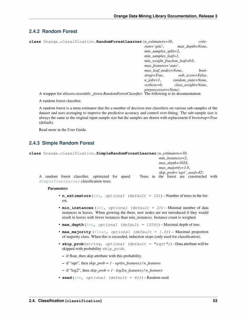
Orange Data Mining Library Documentation, Release 3
2.4.2 Random Forest
class Orange.classification.RandomForestLearner(n_estimators=10, crite-rion=’gini’, max_depth=None,min_samples_split=2,min_samples_leaf=1,min_weight_fraction_leaf=0.0,max_features=’auto’,max_leaf_nodes=None, boot-strap=True, oob_score=False,n_jobs=1, random_state=None,verbose=0, class_weight=None,preprocessors=None)
A wrapper for sklearn.ensemble._forest.RandomForestClassifier. The following is its documentation:
A random forest classifier.
A random forest is a meta estimator that fits a number of decision tree classifiers on various sub-samples of thedataset and uses averaging to improve the predictive accuracy and control over-fitting. The sub-sample size isalways the same as the original input sample size but the samples are drawn with replacement if bootstrap=True(default).
Read more in the User Guide.
2.4.3 Simple Random Forest
class Orange.classification.SimpleRandomForestLearner(n_estimators=10,min_instances=2,max_depth=1024,max_majority=1.0,skip_prob=’sqrt’, seed=42)
A random forest classifier, optimized for speed. Trees in the forest are constructed withSimpleTreeLearner classification trees.
Parameters
• n_estimators (int, optional (default = 10)) – Number of trees in the for-est.
• min_instances (int, optional (default = 2)) – Minimal number of datainstances in leaves. When growing the three, new nodes are not introduced if they wouldresult in leaves with fewer instances than min_instances. Instance count is weighed.
• max_depth (int, optional (default = 1024)) – Maximal depth of tree.
• max_majority (float, optional (default = 1.0)) – Maximal proportionof majority class. When this is exceeded, induction stops (only used for classification).
• skip_prob (string, optional (default = "sqrt")) – Data attribute will beskipped with probability skip_prob.
– if float, then skip attribute with this probability.
– if “sqrt”, then skip_prob = 1 - sqrt(n_features) / n_features
– if “log2”, then skip_prob = 1 - log2(n_features) / n_features
• seed (int, optional (default = 42)) – Random seed.
2.4. Classification (classification) 53

Orange Data Mining Library Documentation, Release 3
fit_storage(data)Default implementation of fit_storage defaults to calling fit. Derived classes must define fit_storage or fit
2.4.4 Softmax Regression
class Orange.classification.SoftmaxRegressionLearner(lambda_=1.0, preproces-sors=None, **fmin_args)
L2 regularized softmax regression classifier. Uses the L-BFGS algorithm to minimize the categorical cross en-tropy cost with L2 regularization. This model is suitable when dealing with a multi-class classification problem.
When using this learner you should:
• choose a suitable regularization parameter lambda_,
• consider using many logistic regression models (one for each value of the class variable) instead of softmaxregression.
Parameters
• lambda_ (float, optional (default=1.0)) – Regularization parameter. It con-trols trade-off between fitting the data and keeping parameters small. Higher values oflambda_ force parameters to be smaller.
• preprocessors (list, optional) – Preprocessors are applied to data before train-ing or testing. Default preprocessors: Defaults to [RemoveNaNClasses(), RemoveNaN-Columns(), Impute(), Continuize(), Normalize()]
– remove columns with all values as NaN
– replace NaN values with suitable values
– continuize all discrete attributes,
– transform the dataset so that the columns are on a similar scale,
• fmin_args (dict, optional) – Parameters for L-BFGS algorithm.
2.4.5 k-Nearest Neighbors
class Orange.classification.KNNLearner(n_neighbors=5, metric=’euclidean’,weights=’uniform’, algorithm=’auto’, met-ric_params=None, preprocessors=None)
A wrapper for sklearn.neighbors._classification.KNeighborsClassifier. The following is its documentation:
Classifier implementing the k-nearest neighbors vote.
Read more in the User Guide.
2.4.6 Naive Bayes
class Orange.classification.NaiveBayesLearner(preprocessors=None)Naive Bayes classifier. Works only with discrete attributes. By default, continuous attributes are discretized.
Parameters preprocessors (list, optional (default="[Orange.preprocess.Discretize]")) – An ordered list of preprocessors applied to databefore training or testing.
54 Chapter 2. Reference

Orange Data Mining Library Documentation, Release 3
fit_storage(table)Default implementation of fit_storage defaults to calling fit. Derived classes must define fit_storage or fit
The following code loads lenses dataset (four discrete attributes and discrete class), constructs naive Bayesian learner,uses it on the entire dataset to construct a classifier, and then applies classifier to the first three data instances:
>>> import Orange>>> lenses = Orange.data.Table('lenses')>>> nb = Orange.classification.NaiveBayesLearner()>>> classifier = nb(lenses)>>> classifier(lenses[0:3], True)array([[ 0.04358755, 0.82671726, 0.12969519],
[ 0.17428279, 0.20342097, 0.62229625],[ 0.18633359, 0.79518516, 0.01848125]])
For datasets that include continuous attributes,
2.4.7 Support Vector Machines
class Orange.classification.SVMLearner(C=1.0, kernel=’rbf’, degree=3, gamma=’auto’,coef0=0.0, shrinking=True, probability=False,tol=0.001, cache_size=200, max_iter=-1, prepro-cessors=None)
A wrapper for sklearn.svm._classes.SVC. The following is its documentation:
C-Support Vector Classification.
The implementation is based on libsvm. The fit time scales at least quadratically with the number of samplesand may be impractical beyond tens of thousands of samples. For large datasets consider using sklearn.svm.LinearSVC or sklearn.linear_model.SGDClassifier instead, possibly after a sklearn.kernel_approximation.Nystroem transformer.
The multiclass support is handled according to a one-vs-one scheme.
For details on the precise mathematical formulation of the provided kernel functions and how gamma, coef0 anddegree affect each other, see the corresponding section in the narrative documentation: svm_kernels.
Read more in the User Guide.
2.4.8 Linear Support Vector Machines
class Orange.classification.LinearSVMLearner(penalty=’l2’, loss=’squared_hinge’,dual=True, tol=0.0001, C=1.0,multi_class=’ovr’, fit_intercept=True,intercept_scaling=True, ran-dom_state=None, preprocessors=None)
A wrapper for sklearn.svm._classes.LinearSVC. The following is its documentation:
Linear Support Vector Classification.
Similar to SVC with parameter kernel=’linear’, but implemented in terms of liblinear rather than libsvm, so ithas more flexibility in the choice of penalties and loss functions and should scale better to large numbers ofsamples.
This class supports both dense and sparse input and the multiclass support is handled according to a one-vs-the-rest scheme.
Read more in the User Guide.
2.4. Classification (classification) 55
Orange Data Mining Library Documentation, Release 3
2.4.9 Nu-Support Vector Machines
class Orange.classification.NuSVMLearner(nu=0.5, kernel=’rbf’, degree=3, gamma=’auto’,coef0=0.0, shrinking=True, probability=False,tol=0.001, cache_size=200, max_iter=-1, prepro-cessors=None)
A wrapper for sklearn.svm._classes.NuSVC. The following is its documentation:
Nu-Support Vector Classification.
Similar to SVC but uses a parameter to control the number of support vectors.
The implementation is based on libsvm.
Read more in the User Guide.
2.4.10 Classification Tree
Orange includes three implemenations of classification trees. TreeLearner is home-grown and properly handles multi-nominal and missing values. The one from scikit-learn, SklTreeLearner, is faster. Another home-grown, SimpleTree-Learner, is simpler and stil faster.
class Orange.classification.TreeLearner(*args, binarize=False, max_depth=None,min_samples_leaf=1, min_samples_split=2,sufficient_majority=0.95, preprocessors=None,**kwargs)
Tree inducer with proper handling of nominal attributes and binarization.
The inducer can handle missing values of attributes and target. For discrete attributes with more than twopossible values, each value can get a separate branch (binarize=False), or values can be grouped into twogroups (binarize=True, default).
The tree growth can be limited by the required number of instances for internal nodes and for leafs, the sufficientproportion of majority class, and by the maximal depth of the tree.
If the tree is not binary, it can contain zero-branches.
Parameters
• binarize (bool) – if True the inducer will find optimal split into two subsets for valuesof discrete attributes. If False (default), each value gets its branch.
• min_samples_leaf (float) – the minimal number of data instances in a leaf
• min_samples_split (float) – the minimal nubmer of data instances that is split intosubgroups
• max_depth (int) – the maximal depth of the tree
• sufficient_majority (float) – a majority at which the data is not split further
Returns instance of OrangeTreeModel
build_tree(data, active_inst, level=1)Induce a tree from the given data
Returns root node (Node)
fit_storage(data)Default implementation of fit_storage defaults to calling fit. Derived classes must define fit_storage or fit
56 Chapter 2. Reference
Orange Data Mining Library Documentation, Release 3
class Orange.classification.SklTreeLearner(criterion=’gini’, splitter=’best’,max_depth=None, min_samples_split=2,min_samples_leaf=1, max_features=None,random_state=None, max_leaf_nodes=None,preprocessors=None)
Wrapper for SKL’s tree inducer
2.4.11 Simple Tree
class Orange.classification.SimpleTreeLearner(min_instances=2, max_depth=1024,max_majority=1.0, skip_prob=0.0,bootstrap=False, seed=42)
Classification or regression tree learner. Uses gain ratio for classification and mean square error for regression.This learner was developed to speed-up random forest construction, but can also be used as a standalone treelearner.
min_instances [int, optional (default = 2)] Minimal number of data instances in leaves. When growing thethree, new nodes are not introduced if they would result in leaves with fewer instances than min_instances.Instance count is weighed.
max_depth [int, optional (default = 1024)] Maximal depth of tree.
max_majority [float, optional (default = 1.0)] Maximal proportion of majority class. When this is exceeded,induction stops (only used for classification).
skip_prob [string, optional (default = 0.0)] Data attribute will be skipped with probability skip_prob.
• if float, then skip attribute with this probability.
• if “sqrt”, then skip_prob = 1 - sqrt(n_features) / n_features
• if “log2”, then skip_prob = 1 - log2(n_features) / n_features
bootstrap [data table, optional (default = False)] A bootstrap dataset.
seed [int, optional (default = 42)] Random seed.
fit_storage(data)Default implementation of fit_storage defaults to calling fit. Derived classes must define fit_storage or fit
2.4.12 Majority Classifier
class Orange.classification.MajorityLearner(preprocessors=None)A majority classifier. Always returns most frequent class from the training set, regardless of the attribute valuesfrom the test data instance. Returns class value distribution if class probabilities are requested. Can be used asa baseline when comparing classifiers.
In the special case of uniform class distribution within the training data, class value is selected randomly. Inorder to produce consistent results on the same dataset, this value is selected based on hash of the class vector.
fit_storage(dat)Default implementation of fit_storage defaults to calling fit. Derived classes must define fit_storage or fit
2.4. Classification (classification) 57

Orange Data Mining Library Documentation, Release 3
2.4.13 Neural Network
class Orange.classification.NNClassificationLearner(hidden_layer_sizes=(100,), activation=’relu’,solver=’adam’, alpha=0.0001,batch_size=’auto’, learn-ing_rate=’constant’,learning_rate_init=0.001,power_t=0.5, max_iter=200,shuffle=True, ran-dom_state=None,tol=0.0001, verbose=False,warm_start=False, mo-mentum=0.9, nes-terovs_momentum=True,early_stopping=False, valida-tion_fraction=0.1, beta_1=0.9,beta_2=0.999, epsilon=1e-08,preprocessors=None)
A wrapper for Orange.classification.neural_network.MLPClassifierWCallback. The following is its documen-tation:
Multi-layer Perceptron classifier.
This model optimizes the log-loss function using LBFGS or stochastic gradient descent.
New in version 0.18.
2.4.14 CN2 Rule Induction
Induction of rules works by finding a rule that covers some learning instances, removing these instances, and repeatingthis until all instances are covered. Rules are scored by heuristics such as impurity of class distribution of coveredinstances. The module includes common rule-learning algorithms, and allows for replacing rule search strategies,scoring and other components.
class Orange.classification.rules.CN2Learner(preprocessors=None, base_rules=None)Classic CN2 inducer that constructs a list of ordered rules. To evaluate found hypotheses, entropy measure isused. Returns a CN2Classifier if called with data.
References
“The CN2 Induction Algorithm”, Peter Clark and Tim Niblett, Machine Learning Journal, 3 (4), pp261-283,(1989)
fit_storage(data)Default implementation of fit_storage defaults to calling fit. Derived classes must define fit_storage or fit
class Orange.classification.rules.CN2UnorderedLearner(preprocessors=None,base_rules=None)
Construct a set of unordered rules.
Rules are learnt for each class individually and scored by the relative frequency of the class corrected by theLaplace correction. After adding a rule, only the covered examples of that class are removed.
The code below loads the iris dataset (four continuous attributes and a discrete class) and fits the learner.
58 Chapter 2. Reference
Orange Data Mining Library Documentation, Release 3
import Orange
data = Orange.data.Table("iris")learner = Orange.classification.CN2UnorderedLearner()
# consider up to 10 solution streams at one timelearner.rule_finder.search_algorithm.beam_width = 10
# continuous value space is constrained to reduce computation timelearner.rule_finder.search_strategy.constrain_continuous = True
# found rules must cover at least 15 exampleslearner.rule_finder.general_validator.min_covered_examples = 15
# found rules may combine at most 2 selectors (conditions)learner.rule_finder.general_validator.max_rule_length = 2
classifier = learner(data)
References
“Rule Induction with CN2: Some Recent Improvements”, Peter Clark and Robin Boswell, Machine Learning -Proceedings of the 5th European Conference (EWSL-91), pp151-163, 1991
fit_storage(data)Default implementation of fit_storage defaults to calling fit. Derived classes must define fit_storage or fit
class Orange.classification.rules.CN2SDLearner(preprocessors=None,base_rules=None)
Ordered CN2SD inducer that constructs a list of ordered rules. To evaluate found hypotheses, Weighted relativeaccuracy measure is used. Returns a CN2SDClassifier if called with data.
In this setting, ordered rule induction refers exclusively to finding best rule conditions and assigning the majorityclass in the rule head (target class is set to None). To later predict instances, rules will be regarded as unordered.
Notes
A weighted covering algorithm is applied, in which subsequently induced rules also represent interesting andsufficiently large subgroups of the population. Covered positive examples are not deleted from the learning set,rather their weight is reduced.
The algorithm demonstrates how classification rule learning (predictive induction) can be adapted to subgroupdiscovery, a task at the intersection of predictive and descriptive induction.
References
“Subgroup Discovery with CN2-SD”, Nada Lavrac et al., Journal of Machine Learning Research 5 (2004),153-188, 2004
fit_storage(data)Default implementation of fit_storage defaults to calling fit. Derived classes must define fit_storage or fit
class Orange.classification.rules.CN2SDUnorderedLearner(preprocessors=None,base_rules=None)
Unordered CN2SD inducer that constructs a set of unordered rules. To evaluate found hypotheses, Weightedrelative accuracy measure is used. Returns a CN2SDUnorderedClassifier if called with data.
2.4. Classification (classification) 59

Orange Data Mining Library Documentation, Release 3
Notes
A weighted covering algorithm is applied, in which subsequently induced rules also represent interesting andsufficiently large subgroups of the population. Covered positive examples are not deleted from the learning set,rather their weight is reduced.
The algorithm demonstrates how classification rule learning (predictive induction) can be adapted to subgroupdiscovery, a task at the intersection of predictive and descriptive induction.
References
“Subgroup Discovery with CN2-SD”, Nada Lavrac et al., Journal of Machine Learning Research 5 (2004),153-188, 2004
fit_storage(data)Default implementation of fit_storage defaults to calling fit. Derived classes must define fit_storage or fit
2.4.15 Calibration and threshold optimization
class Orange.classification.calibration.ThresholdClassifier(base_model, thresh-old)
A model that wraps a binary model and sets a different threshold.
The target class is the class with index 1. A data instances is classified to class 1 it the probability of this classequals or exceeds the threshold
base_modelbase mode
Type Orange.classification.Model
thresholddecision threshold
Type float
class Orange.classification.calibration.ThresholdLearner(base_learner, thresh-old_criterion=0)
A learner that runs another learner and then finds the optimal threshold for CA or F1 on the training data.
base_leanerbase learner
Type Learner
threshold_criterionThresholdLearner.OptimizeCA or ThresholdLearner.OptimizeF1
Type int
fit_storage(data)Induce a model using the provided base_learner, compute probabilities on training data and the find theoptimal decision thresholds. In case of ties, select the threshold that is closest to 0.5.
class Orange.classification.calibration.CalibratedClassifier(base_model, cali-brators)
A model that wraps another model and recalibrates probabilities
base_modelbase mode
60 Chapter 2. Reference
Orange Data Mining Library Documentation, Release 3
Type Mode
calibratorslist of functions that get a vector of probabilities and return calibrated probabilities
Type list of callable
class Orange.classification.calibration.CalibratedLearner(base_learner, calibra-tion_method=0)
Probability calibration for learning algorithms
This learner that wraps another learner, so that after training, it predicts the probabilities on training data andcalibrates them using sigmoid or isotonic calibration. It then returns a CalibratedClassifier.
base_learnerbase learner
Type Learner
calibration_methodCalibratedLearner.Sigmoid or CalibratedLearner.Isotonic
Type int
fit_storage(data)Induce a model using the provided base_learner, compute probabilities on training data and use scipy’s_SigmoidCalibration or IsotonicRegression to prepare calibrators.
2.5 Regression (regression)
2.5.1 Linear Regression
Linear regression is a statistical regression method which tries to predict a value of a continuous response (class)variable based on the values of several predictors. The model assumes that the response variable is a linear combinationof the predictors, the task of linear regression is therefore to fit the unknown coefficients.
Example
>>> from Orange.regression.linear import LinearRegressionLearner>>> mpg = Orange.data.Table('auto-mpg')>>> mean_ = LinearRegressionLearner()>>> model = mean_(mpg[40:110])>>> print(model)LinearModel LinearRegression(copy_X=True, fit_intercept=True, normalize=False)>>> mpg[20]Value('mpg', 25.0)>>> model(mpg[0])Value('mpg', 24.6)
class Orange.regression.linear.LinearRegressionLearner(preprocessors=None)A wrapper for sklearn.linear_model._base.LinearRegression. The following is its documentation:
Ordinary least squares Linear Regression.
LinearRegression fits a linear model with coefficients w = (w1, . . . , wp) to minimize the residual sum of squaresbetween the observed targets in the dataset, and the targets predicted by the linear approximation.
2.5. Regression (regression) 61
Orange Data Mining Library Documentation, Release 3
class Orange.regression.linear.RidgeRegressionLearner(alpha=1.0,fit_intercept=True, nor-malize=False, copy_X=True,max_iter=None, tol=0.001,solver=’auto’, preproces-sors=None)
A wrapper for sklearn.linear_model._ridge.Ridge. The following is its documentation:
Linear least squares with l2 regularization.
Minimizes the objective function:
||y - Xw||^2_2 + alpha * ||w||^2_2
This model solves a regression model where the loss function is the linear least squares function and regulariza-tion is given by the l2-norm. Also known as Ridge Regression or Tikhonov regularization. This estimator hasbuilt-in support for multi-variate regression (i.e., when y is a 2d-array of shape (n_samples, n_targets)).
Read more in the User Guide.
class Orange.regression.linear.LassoRegressionLearner(alpha=1.0,fit_intercept=True, nor-malize=False, precom-pute=False, copy_X=True,max_iter=1000, tol=0.0001,warm_start=False, pos-itive=False, preproces-sors=None)
A wrapper for sklearn.linear_model._coordinate_descent.Lasso. The following is its documentation:
Linear Model trained with L1 prior as regularizer (aka the Lasso)
The optimization objective for Lasso is:
(1 / (2 * n_samples)) * ||y - Xw||^2_2 + alpha * ||w||_1
Technically the Lasso model is optimizing the same objective function as the Elastic Net with l1_ratio=1.0(no L2 penalty).
Read more in the User Guide.
class Orange.regression.linear.SGDRegressionLearner(loss=’squared_loss’,penalty=’l2’, al-pha=0.0001, l1_ratio=0.15,fit_intercept=True, max_iter=5,tol=0.001, shuffle=True, ep-silon=0.1, n_jobs=1, ran-dom_state=None, learn-ing_rate=’invscaling’,eta0=0.01, power_t=0.25,class_weight=None,warm_start=False, av-erage=False, preproces-sors=None)
A wrapper for sklearn.linear_model._stochastic_gradient.SGDRegressor. The following is its documentation:
Linear model fitted by minimizing a regularized empirical loss with SGD
SGD stands for Stochastic Gradient Descent: the gradient of the loss is estimated each sample at a time and themodel is updated along the way with a decreasing strength schedule (aka learning rate).
62 Chapter 2. Reference

Orange Data Mining Library Documentation, Release 3
The regularizer is a penalty added to the loss function that shrinks model parameters towards the zero vectorusing either the squared euclidean norm L2 or the absolute norm L1 or a combination of both (Elastic Net). Ifthe parameter update crosses the 0.0 value because of the regularizer, the update is truncated to 0.0 to allow forlearning sparse models and achieve online feature selection.
This implementation works with data represented as dense numpy arrays of floating point values for the features.
Read more in the User Guide.
class Orange.regression.linear.LinearModel(skl_model)
2.5.2 Polynomial
Polynomial model is a wrapper that constructs polynomial features of a specified degree and learns a model on them.
class Orange.regression.linear.PolynomialLearner(learner=LinearRegressionLearner(),degree=2, preprocessors=None)
Generate polynomial features and learn a prediction model
Parameters
• learner (LearnerRegression) – learner to be fitted on the transformed features
• degree (int) – degree of used polynomial
• preprocessors (List[Preprocessor]) – preprocessors to be applied on the databefore learning
2.5.3 Mean
Mean model predicts the same value (usually the distribution mean) for all data instances. Its accuracy can serve as abaseline for other regression models.
The model learner (MeanLearner) computes the mean of the given data or distribution. The model is stored as aninstance of MeanModel.
Example
>>> from Orange.data import Table>>> from Orange.regression import MeanLearner>>> data = Table('auto-mpg')>>> learner = MeanLearner()>>> model = learner(data)>>> print(model)MeanModel(23.51457286432161)>>> model(data[:4])array([ 23.51457286, 23.51457286, 23.51457286, 23.51457286])
class Orange.regression.MeanLearner(preprocessors=None)Fit a regression model that returns the average response (class) value.
fit_storage(data)Construct a MeanModel by computing the mean value of the given data.
Parameters data (Orange.data.Table) – data table
Returns regression model, which always returns mean value
Return type MeanModel
2.5. Regression (regression) 63
Orange Data Mining Library Documentation, Release 3
2.5.4 Random Forest
class Orange.regression.RandomForestRegressionLearner(n_estimators=10,criterion=’mse’,max_depth=None,min_samples_split=2,min_samples_leaf=1,min_weight_fraction_leaf=0.0,max_features=’auto’,max_leaf_nodes=None,bootstrap=True,oob_score=False, n_jobs=1,random_state=None,verbose=0, preproces-sors=None)
A wrapper for sklearn.ensemble._forest.RandomForestRegressor. The following is its documentation:
A random forest regressor.
A random forest is a meta estimator that fits a number of classifying decision trees on various sub-samples of thedataset and uses averaging to improve the predictive accuracy and control over-fitting. The sub-sample size isalways the same as the original input sample size but the samples are drawn with replacement if bootstrap=True(default).
Read more in the User Guide.
2.5.5 Simple Random Forest
class Orange.regression.SimpleRandomForestLearner(n_estimators=10, min_instances=2,max_depth=1024,max_majority=1.0,skip_prob=’sqrt’, seed=42)
A random forest regressor, optimized for speed. Trees in the forest are constructed withSimpleTreeLearner classification trees.
Parameters
• n_estimators (int, optional (default = 10)) – Number of trees in the for-est.
• min_instances (int, optional (default = 2)) – Minimal number of datainstances in leaves. When growing the three, new nodes are not introduced if they wouldresult in leaves with fewer instances than min_instances. Instance count is weighed.
• max_depth (int, optional (default = 1024)) – Maximal depth of tree.
• max_majority (float, optional (default = 1.0)) – Maximal proportionof majority class. When this is exceeded, induction stops (only used for classification).
• skip_prob (string, optional (default = "sqrt")) – Data attribute will beskipped with probability skip_prob.
– if float, then skip attribute with this probability.
– if “sqrt”, then skip_prob = 1 - sqrt(n_features) / n_features
– if “log2”, then skip_prob = 1 - log2(n_features) / n_features
• seed (int, optional (default = 42)) – Random seed.
64 Chapter 2. Reference

Orange Data Mining Library Documentation, Release 3
fit_storage(data)Default implementation of fit_storage defaults to calling fit. Derived classes must define fit_storage or fit
2.5.6 Regression Tree
Orange includes two implemenations of regression tres: a home-grown one, and one from scikit-learn. The formerproperly handles multinominal and missing values, and the latter is faster.
class Orange.regression.TreeLearner(*args, binarize=False, min_samples_leaf=1,min_samples_split=2, max_depth=None, **kwargs)
Tree inducer with proper handling of nominal attributes and binarization.
The inducer can handle missing values of attributes and target. For discrete attributes with more than twopossible values, each value can get a separate branch (binarize=False), or values can be grouped into twogroups (binarize=True, default).
The tree growth can be limited by the required number of instances for internal nodes and for leafs, and by themaximal depth of the tree.
If the tree is not binary, it can contain zero-branches.
Parameters
• binarize – if True the inducer will find optimal split into two subsets for values of discreteattributes. If False (default), each value gets its branch.
• min_samples_leaf – the minimal number of data instances in a leaf
• min_samples_split – the minimal number of data instances that is split into subgroups
• max_depth – the maximal depth of the tree
Returns
Return type instance of OrangeTreeModel
build_tree(data, active_inst, level=1)Induce a tree from the given data
Returns root node (Node)
fit_storage(data)Default implementation of fit_storage defaults to calling fit. Derived classes must define fit_storage or fit
class Orange.regression.SklTreeRegressionLearner(criterion=’mse’, split-ter=’best’, max_depth=None,min_samples_split=2,min_samples_leaf=1,max_features=None,random_state=None,max_leaf_nodes=None, prepro-cessors=None)
A wrapper for sklearn.tree._classes.DecisionTreeRegressor. The following is its documentation:
A decision tree regressor.
Read more in the User Guide.
2.5. Regression (regression) 65

Orange Data Mining Library Documentation, Release 3
2.5.7 Neural Network
class Orange.regression.NNRegressionLearner(hidden_layer_sizes=(100, ), acti-vation=’relu’, solver=’adam’, al-pha=0.0001, batch_size=’auto’,learning_rate=’constant’, learn-ing_rate_init=0.001, power_t=0.5,max_iter=200, shuffle=True, ran-dom_state=None, tol=0.0001, ver-bose=False, warm_start=False, momen-tum=0.9, nesterovs_momentum=True,early_stopping=False, valida-tion_fraction=0.1, beta_1=0.9,beta_2=0.999, epsilon=1e-08, prepro-cessors=None)
A wrapper for Orange.regression.neural_network.MLPRegressorWCallback. The following is its documenta-tion:
Multi-layer Perceptron regressor.
This model optimizes the squared-loss using LBFGS or stochastic gradient descent.
New in version 0.18.
2.6 Clustering (clustering)
2.6.1 Hierarchical (hierarchical)
Example
The following example shows clustering of the Iris data with distance matrix computed with the Orange.distance.Euclidean distance and clustering using average linkage.
>>> from Orange import data, distance>>> from Orange.clustering import hierarchical>>> data = data.Table('iris')>>> dist_matrix = distance.Euclidean(data)>>> hierar = hierarchical.HierarchicalClustering(n_clusters=3)>>> hierar.linkage = hierarchical.AVERAGE>>> hierar.fit(dist_matrix)>>> hierar.labelsarray([ 1., 1., 1., 1., 1., 1., 1., 1., 1., 1., 1., 1., 1.,
1., 1., 1., 1., 1., 1., 1., 1., 1., 1., 1., 1., 1.,1., 1., 1., 1., 1., 1., 1., 1., 1., 1., 1., 1., 1.,1., 1., 1., 1., 1., 1., 1., 1., 1., 1., 1., 0., 0.,0., 0., 0., 0., 0., 0., 0., 0., 0., 0., 0., 0., 0.,0., 0., 0., 0., 0., 0., 0., 0., 0., 0., 0., 0., 0.,0., 0., 0., 0., 0., 0., 0., 0., 0., 0., 0., 0., 0.,0., 0., 0., 0., 0., 0., 0., 0., 0., 2., 0., 2., 2.,2., 2., 0., 2., 2., 2., 2., 2., 2., 0., 0., 2., 2.,2., 2., 0., 2., 0., 2., 0., 2., 2., 0., 0., 2., 2.,2., 2., 2., 0., 2., 2., 2., 2., 0., 2., 2., 2., 0.,2., 2., 2., 0., 2., 2., 0.])
66 Chapter 2. Reference
Orange Data Mining Library Documentation, Release 3
Hierarchical Clustering
class Orange.clustering.hierarchical.HierarchicalClustering(n_clusters=2, link-age=’average’)
2.7 Distance (distance)
The following example demonstrates how to compute distances between all data instances from Iris:
>>> from Orange.data import Table>>> from Orange.distance import Euclidean>>> iris = Table('iris')>>> dist_matrix = Euclidean(iris)>>> # Distance between first two examples>>> dist_matrix.X[0, 1]0.53851648
To compute distances between all columns, we set axis to 0.
>>> Euclidean(iris, axis=0)DistMatrix([[ 0. , 36.17927584, 28.9542743 , 57.1913455 ],
[ 36.17927584, 0. , 25.73382987, 25.81259383],[ 28.9542743 , 25.73382987, 0. , 33.87270287],[ 57.1913455 , 25.81259383, 33.87270287, 0. ]])
Finally, we can compute distances between all pairs of rows from two tables.
>>> iris1 = iris[:100]>>> iris2 = iris[100:]>>> dist = Euclidean(iris_even, iris_odd)>>> dist.shape(75, 100)
Most metrics can be fit on training data to normalize values and handle missing data. We do so by calling the con-structor without arguments or with parameters, such as normalize, and then pass the data to method fit.
>>> dist_model = Euclidean(normalize=True).fit(iris1)>>> dist = dist_model(iris2[:3])>>> distDistMatrix([[ 0. , 1.36778277, 1.11352233],
[ 1.36778277, 0. , 1.57810546],[ 1.11352233, 1.57810546, 0. ]])
The above distances are computed on the first three rows of iris2, normalized by means and variances computed fromiris1.
Here are five closest neighbors of iris2[0] from iris1:
>>> dist0 = dist_model(iris1, iris2[0])>>> neigh_idx = np.argsort(dist0.flatten())[:5]>>> iris1[neigh_idx][[5.900, 3.200, 4.800, 1.800 | Iris-versicolor],[6.700, 3.000, 5.000, 1.700 | Iris-versicolor],[6.300, 3.300, 4.700, 1.600 | Iris-versicolor],[6.000, 3.400, 4.500, 1.600 | Iris-versicolor],
(continues on next page)
2.7. Distance (distance) 67

Orange Data Mining Library Documentation, Release 3
(continued from previous page)
[6.400, 3.200, 4.500, 1.500 | Iris-versicolor]]
All distances share a common interface.
class Orange.distance.DistanceBase class for construction of distances models (DistanceModel).
Distances can be computed between all pairs of rows in one table, or between pairs where one row is from onetable and one from another.
If axis is set to 0, the class computes distances between all pairs of columns in a table. Distances betweencolumns from separate tables are probably meaningless, thus unsupported.
The class can be used as follows:
• Constructor is called only with keyword argument axis that specifies the axis over which the distances arecomputed, and with other subclass-specific keyword arguments.
• Next, we call the method fit(data) to produce an instance of DistanceModel; the instance stores any pa-rameters needed for computation of distances, such as statistics for normalization and handling of missingdata.
• We can then call the DistanceModel with data to compute the distance between its rows or columns,or with two data tables to compute distances between all pairs of rows.
The second, shorter way to use this class is to call the constructor with one or two data tables and any additionalkeyword arguments. Constructor will execute the above steps and return DistMatrix. Such usage is here forbackward compatibility, practicality and efficiency.
Parameters
• e1 (Table or Instance or np.ndarray or None) – data on which to train the modeland compute the distances
• e2 (Table or Instance or np.ndarray or None) – if present, the class computesdistances with pairs coming from the two tables
• axis (int) – axis over which the distances are computed, 1 (default) for rows, 0 forcolumns
• impute (bool) – if True (default is False), nans in the computed distances are replacedwith zeros, and infs with very large numbers.
• callback (callable or None) – callback function
axisaxis over which the distances are computed, 1 (default) for rows, 0 for columns
Type int
imputeif True (default is False), nans in the computed distances are replaced with zeros, and infs with very largenumbers.
Type bool
normalizeif True, columns are normalized before computation. This attribute applies only if the distance supportsnormalization.
Type bool
68 Chapter 2. Reference

Orange Data Mining Library Documentation, Release 3
The capabilities of the metrics are described with class attributes.
If class attribute supports_discrete is True, the distance also uses discrete attributes to compute row distances.The use of discrete attributes depends upon the type of distance; e.g. Jaccard distance observes whether thevalue is zero or non-zero, while Euclidean and Manhattan distance observes whether a pair of values is same ordifferent.
Class attribute supports_missing indicates that the distance can cope with missing data. In such cases, lettingthe distance handle it should be preferred over pre-imputation of missing values.
Class attribute supports_normalization indicates that the constructor accepts an argument normalize. If set toTrue, the metric will attempt to normalize the values in a sense that each attribute will have equal influence.For instance, the Euclidean distance subtract the mean and divides the result by the deviation, while Manhattandistance uses the median and MAD.
If class attribute supports_sparse is True, the class will handle sparse data. Currently, all classes that do handleit rely on fallbacks to SKL metrics. These, however, do not support discrete data and missing values, and willfail silently.
2.7.1 Handling discrete and missing data
Discrete data is handled as appropriate for the particular distance. For instance, the Euclidean distance treats a pairof values as either the same or different, contributing either 0 or 1 to the squared sum of differences. In other cases –particularly in Jaccard and cosine distance, discrete values are treated as zero or non-zero.
Missing data is not simply imputed. We assume that values of each variable are distributed by some unknown distri-bution and compute - without assuming a particular distribution shape - the expected distance. For instance, for theEuclidean distance it turns out that the expected squared distance between a known and a missing value equals thesquare of the known value’s distance from the mean of the missing variable, plus its variance.
2.7.2 Supported distances
Euclidean distance
For numeric values, the Euclidean distance is the square root of sums of squares of pairs of values from rows orcolumns. For discrete values, 1 is added if the two values are different.
To put all numeric data on the same scale, and in particular when working with a mixture of numeric and discrete data,it is recommended to enable normalization by adding normalize=True to the constructor. With this, numeric valuesare normalized by subtracting their mean and divided by deviation multiplied by the square root of two. The mean anddeviation are computed on the training data, if the fit method is used. When computing distances between two tablesand without explicitly calling fit, means and variances are computed from the first table only. Means and variances arealways computed from columns, disregarding the axis over which we compute the distances, since columns representvariables and hence come from a certain distribution.
As described above, the expected squared difference between a known and a missing value equals the squared differ-ence between the known value and the mean, plus the variance. The squared difference between two unknown valuesequals twice the variance.
For normalized data, the difference between a known and missing numeric value equals the square of the known value+ 0.5. The difference between two missing values is 1.
For discrete data, the expected difference between a known and a missing value equals the probablity that the twovalues are different, which is 1 minus the probability of the known value. If both values are missing, the probabilityof them being different equals 1 minus the sum of squares of all probabilities (also known as the Gini index).
2.7. Distance (distance) 69

Orange Data Mining Library Documentation, Release 3
Manhattan distance
Manhattan distance is the sum of absolute pairwise distances.
Normalization and treatment of missing values is similar as in the Euclidean distance, except that medians and medianabsolute distance from the median (MAD) are used instead of means and deviations.
For discrete values, distances are again 0 or 1, hence the Manhattan distance for discrete columns is the same as theEuclidean.
Cosine distance
Cosine similarity is the dot product divided by the product of lengths (where the length is the square of dot product ofa row/column with itself). Cosine distance is computed by subtracting the similarity from one.
In calculation of dot products, missing values are replaced by means. In calculation of lengths, the contribution of amissing value equals the square of the mean plus the variance. (The difference comes from the fact that in the formercase the missing values are independent.)
Non-zero discrete values are replaced by 1. This introduces the notion of a “base value”, which is the first in the listof possible values. In most cases, this will only make sense for indicator (i.e. two-valued, boolean attributes).
Cosine distance does not support any column-wise normalization.
Jaccard distance
Jaccard similarity between two sets is defined as the size of their intersection divided by the size of the union. Jaccarddistance is computed by subtracting the similarity from one.
In Orange, attribute values are interpreted as membership indicator. In row-wise distances, columns are interpreted assets, and non-zero values in a row (including negative values of numeric features) indicate that the row belongs to theparticular sets. In column-wise distances, rows are sets and values indicate the sets to which the column belongs.
For missing values, relative frequencies from the training data are used as probabilities for belonging to a set. Thatis, for row-wise distances, we compute the relative frequency of non-zero values in each column, and vice-versa forcolumn-wise distances. For intersection (union) of sets, we then add the probability of belonging to both (any of) thetwo sets instead of adding a 0 or 1.
SpearmanR, AbsoluteSpearmanR, PearsonR, AbsolutePearsonR
The four correlation-based distance measure equal (1 - the correlation coefficient) / 2. For AbsoluteSpearmanR andAbsolutePearsonR, the absolute value of the coefficient is used.
These distances do not handle missing or discrete values.
Mahalanobis distance
Mahalanobis distance is similar to cosine distance, except that the data is projected into the PCA space.
Mahalanobis distance does not handle missing or discrete values.
70 Chapter 2. Reference

Orange Data Mining Library Documentation, Release 3
2.8 Evaluation (evaluation)
2.8.1 Sampling procedures for testing models (testing)
class Orange.evaluation.testing.Results(data=None, *, nmethods=None,nrows=None, nclasses=None, do-main=None, row_indices=None, folds=None,score_by_folds=True, learners=None, mod-els=None, failed=None, actual=None,predicted=None, probabilities=None,store_data=None, store_models=None,train_time=None, test_time=None)
Class for storing predictions in model testing.
dataData used for testing.
Type Optional[Table]
modelsA list of induced models.
Type Optional[List[Model]]
row_indicesIndices of rows in data that were used in testing, stored as a numpy vector of length nrows. Values ofactual[i], predicted[i] and probabilities[i] refer to the target value of instance, that is, the i-th test instanceis data[row_indices[i]], its actual class is actual[i], and the prediction by m-th method is predicted[m, i].
Type np.ndarray
nrowsThe number of test instances (including duplicates); nrows equals the length of row_indices and actual,and the second dimension of predicted and probabilities.
Type int
actualtrue values of target variable in a vector of length nrows.
Type np.ndarray
predictedpredicted values of target variable in an array of shape (number-of-methods, nrows)
Type np.ndarray
probabilitiespredicted probabilities (for discrete target variables) in an array of shape (number-of-methods, nrows,number-of-classes)
Type Optional[np.ndarray]
foldsa list of indices (or slice objects) corresponding to testing data subsets, that is, row_indices[folds[i]] con-tains row indices used in fold i, so data[row_indices[folds[i]]] is the corresponding testing data
Type List[Slice or List[int]]
train_timetraining times of batches
2.8. Evaluation (evaluation) 71

Orange Data Mining Library Documentation, Release 3
Type np.ndarray
test_timetesting times of batches
Type np.ndarray
get_augmented_data(model_names, include_attrs=True, include_predictions=True, in-clude_probabilities=True)
Return the test data table augmented with meta attributes containing predictions, probabilities (if the taskis classification) and fold indices.
Parameters
• model_names (list of str) – names of models
• include_attrs (bool) – if set to False, original attributes are removed
• include_predictions (bool) – if set to False, predictions are not added
• include_probabilities (bool) – if set to False, probabilities are not added
Returns data augmented with predictions, probabilities and fold indices
Return type augmented_data (Orange.data.Table)
split_by_model()Split evaluation results by models.
The method generates instances of Results containing data for single models
class Orange.evaluation.testing.CrossValidation(k=10, stratified=True, ran-dom_state=0, store_data=False,store_models=False, warn-ings=None)
K-fold cross validation
knumber of folds (default: 10)
Type int
random_stateseed for random number generator (default: 0). If set to None, a different seed is used each time
Type int
stratifiedflag deciding whether to perform stratified cross-validation. If True but the class sizes don’t allow it, ituses non-stratified validataion and adds a list warning with a warning message(s) to the Result.
Type bool
get_indices(data)Return a list of arrays of indices of test data instance
For example, in k-fold CV, the result is a list with k elements, each containing approximately len(data) / knonoverlapping indices into data.
This method is abstract and must be implemented in derived classes unless they provide their own imple-mentation of the __call__ method.
Parameters data (Orange.data.Table) – test data
Returns a list of arrays of indices into data
Return type indices (list of np.ndarray)
72 Chapter 2. Reference
Orange Data Mining Library Documentation, Release 3
class Orange.evaluation.testing.CrossValidationFeature(feature=None,store_data=False,store_models=False, warn-ings=None)
Cross validation with folds according to values of a feature.
featurethe feature defining the folds
Type Orange.data.Variable
get_indices(data)Return a list of arrays of indices of test data instance
For example, in k-fold CV, the result is a list with k elements, each containing approximately len(data) / knonoverlapping indices into data.
This method is abstract and must be implemented in derived classes unless they provide their own imple-mentation of the __call__ method.
Parameters data (Orange.data.Table) – test data
Returns a list of arrays of indices into data
Return type indices (list of np.ndarray)
class Orange.evaluation.testing.LeaveOneOut(*, store_data=False, store_models=False)Leave-one-out testing
get_indices(data)Return a list of arrays of indices of test data instance
For example, in k-fold CV, the result is a list with k elements, each containing approximately len(data) / knonoverlapping indices into data.
This method is abstract and must be implemented in derived classes unless they provide their own imple-mentation of the __call__ method.
Parameters data (Orange.data.Table) – test data
Returns a list of arrays of indices into data
Return type indices (list of np.ndarray)
static prepare_arrays(data, indices)Prepare folds, row_indices and actual.
The method is used by __call__. While functional, it may be overriden in subclasses for speed-ups.
Parameters
• data (Orange.data.Table) – data use for testing
• indices (list of vectors) – indices of data instances in each test sample
Returns (np.ndarray): see class documentation row_indices: (np.ndarray): see class documen-tation actual: (np.ndarray): see class documentation
Return type folds
class Orange.evaluation.testing.ShuffleSplit(n_resamples=10, train_size=None,test_size=0.1, stratified=True, ran-dom_state=0, store_data=False,store_models=False)
Test by repeated random sampling
2.8. Evaluation (evaluation) 73
Orange Data Mining Library Documentation, Release 3
n_resamplesnumber of repetitions
Type int
test_sizeIf float, should be between 0.0 and 1.0 and represent the proportion of the dataset to include in the testsplit. If int, represents the absolute number of test samples. If None, the value is set to the complement ofthe train size. By default, the value is set to 0.1. The default will change in version 0.21. It will remain 0.1only if train_size is unspecified, otherwise it will complement the specified train_size. (fromdocumentation of scipy.sklearn.StratifiedShuffleSplit)
Type float, int, None
train_sizefloat, int, or None, default is None If float, should be between 0.0 and 1.0 and represent the propor-tion of the dataset to include in the train split. If int, represents the absolute number of train sam-ples. If None, the value is automatically set to the complement of the test size. (from documentationof scipy.sklearn.StratifiedShuffleSplit)
stratifiedflag deciding whether to perform stratified cross-validation.
Type bool
random_stateseed for random number generator (default: 0). If set to None, a different seed is used each time
Type int
get_indices(data)Return a list of arrays of indices of test data instance
For example, in k-fold CV, the result is a list with k elements, each containing approximately len(data) / knonoverlapping indices into data.
This method is abstract and must be implemented in derived classes unless they provide their own imple-mentation of the __call__ method.
Parameters data (Orange.data.Table) – test data
Returns a list of arrays of indices into data
Return type indices (list of np.ndarray)
class Orange.evaluation.testing.TestOnTestData(*, store_data=False,store_models=False)
Test on separately provided test data
Note that the class has a different signature for __call__.
class Orange.evaluation.testing.TestOnTrainingData(*, store_data=False,store_models=False)
Test on training data
Orange.evaluation.testing.sample(table, n=0.7, stratified=False, replace=False, ran-dom_state=None)
Samples data instances from a data table. Returns the sample and a dataset from input data table that are not inthe sample. Also uses several sampling functions from scikit-learn.
table [data table] A data table from which to sample.
n [float, int (default = 0.7)] If float, should be between 0.0 and 1.0 and represents the proportion of data instancesin the resulting sample. If int, n is the number of data instances in the resulting sample.
74 Chapter 2. Reference

Orange Data Mining Library Documentation, Release 3
stratified [bool, optional (default = False)] If true, sampling will try to consider class values and match distri-bution of class values in train and test subsets.
replace [bool, optional (default = False)] sample with replacement
random_state [int or RandomState] Pseudo-random number generator state used for random sampling.
2.8.2 Scoring methods (scoring)
CA
Orange.evaluation.CA(results=None, **kwargs)A wrapper for sklearn.metrics._classification.accuracy_score. The following is its documentation:
Accuracy classification score.
In multilabel classification, this function computes subset accuracy: the set of labels predicted for a sample mustexactly match the corresponding set of labels in y_true.
Read more in the User Guide.
Precision
Orange.evaluation.Precision(results=None, **kwargs)A wrapper for sklearn.metrics._classification.precision_score. The following is its documentation:
Compute the precision
The precision is the ratio tp / (tp + fp) where tp is the number of true positives and fp the number offalse positives. The precision is intuitively the ability of the classifier not to label as positive a sample that isnegative.
The best value is 1 and the worst value is 0.
Read more in the User Guide.
Recall
Orange.evaluation.Recall(results=None, **kwargs)A wrapper for sklearn.metrics._classification.recall_score. The following is its documentation:
Compute the recall
The recall is the ratio tp / (tp + fn) where tp is the number of true positives and fn the number of falsenegatives. The recall is intuitively the ability of the classifier to find all the positive samples.
The best value is 1 and the worst value is 0.
Read more in the User Guide.
F1
Orange.evaluation.F1(results=None, **kwargs)A wrapper for sklearn.metrics._classification.f1_score. The following is its documentation:
Compute the F1 score, also known as balanced F-score or F-measure
2.8. Evaluation (evaluation) 75
Orange Data Mining Library Documentation, Release 3
The F1 score can be interpreted as a weighted average of the precision and recall, where an F1 score reaches itsbest value at 1 and worst score at 0. The relative contribution of precision and recall to the F1 score are equal.The formula for the F1 score is:
F1 = 2 * (precision * recall) / (precision + recall)
In the multi-class and multi-label case, this is the average of the F1 score of each class with weighting dependingon the average parameter.
Read more in the User Guide.
PrecisionRecallFSupport
Orange.evaluation.PrecisionRecallFSupport(results=None, **kwargs)A wrapper for sklearn.metrics._classification.precision_recall_fscore_support. The following is its documenta-tion:
Compute precision, recall, F-measure and support for each class
The precision is the ratio tp / (tp + fp) where tp is the number of true positives and fp the number offalse positives. The precision is intuitively the ability of the classifier not to label as positive a sample that isnegative.
The recall is the ratio tp / (tp + fn) where tp is the number of true positives and fn the number of falsenegatives. The recall is intuitively the ability of the classifier to find all the positive samples.
The F-beta score can be interpreted as a weighted harmonic mean of the precision and recall, where an F-betascore reaches its best value at 1 and worst score at 0.
The F-beta score weights recall more than precision by a factor of beta. beta == 1.0 means recall andprecision are equally important.
The support is the number of occurrences of each class in y_true.
If pos_label is None and in binary classification, this function returns the average precision, recall andF-measure if average is one of 'micro', 'macro', 'weighted' or 'samples'.
Read more in the User Guide.
AUC
Orange.evaluation.AUC(results=None, **kwargs)${sklpar}
Parameters
• results (Orange.evaluation.Results) – Stored predictions and actual data inmodel testing.
• target (int, optional (default=None)) – Value of class to report.
Log Loss
Orange.evaluation.LogLoss(results=None, **kwargs)${sklpar}
Parameters
76 Chapter 2. Reference

Orange Data Mining Library Documentation, Release 3
• results (Orange.evaluation.Results) – Stored predictions and actual data inmodel testing.
• eps (float) – Log loss is undefined for p=0 or p=1, so probabilities are clipped tomax(eps, min(1 - eps, p)).
• normalize (bool, optional (default=True)) – If true, return the mean lossper sample. Otherwise, return the sum of the per-sample losses.
• sample_weight (array-like of shape = [n_samples], optional) –Sample weights.
Examples
>>> Orange.evaluation.LogLoss(results)array([ 0.3...])
MSE
Orange.evaluation.MSE(results=None, **kwargs)A wrapper for sklearn.metrics._regression.mean_squared_error. The following is its documentation:
Mean squared error regression loss
Read more in the User Guide.
MAE
Orange.evaluation.MAE(results=None, **kwargs)A wrapper for sklearn.metrics._regression.mean_absolute_error. The following is its documentation:
Mean absolute error regression loss
Read more in the User Guide.
R2
Orange.evaluation.R2(results=None, **kwargs)A wrapper for sklearn.metrics._regression.r2_score. The following is its documentation:
R^2 (coefficient of determination) regression score function.
Best possible score is 1.0 and it can be negative (because the model can be arbitrarily worse). A constant modelthat always predicts the expected value of y, disregarding the input features, would get a R^2 score of 0.0.
Read more in the User Guide.
CD diagram
Orange.evaluation.compute_CD(avranks, n, alpha=’0.05’, test=’nemenyi’)Returns critical difference for Nemenyi or Bonferroni-Dunn test according to given alpha (either alpha=”0.05”or alpha=”0.1”) for average ranks and number of tested datasets N. Test can be either “nemenyi” for for Nemenyitwo tailed test or “bonferroni-dunn” for Bonferroni-Dunn test.
2.8. Evaluation (evaluation) 77

Orange Data Mining Library Documentation, Release 3
Orange.evaluation.graph_ranks(avranks, names, cd=None, cdmethod=None, lowv=None,highv=None, width=6, textspace=1, reverse=False, file-name=None, **kwargs)
Draws a CD graph, which is used to display the differences in methods’ performance. See Janez Demsar,Statistical Comparisons of Classifiers over Multiple Data Sets, 7(Jan):1–30, 2006.
Needs matplotlib to work.
The image is ploted on plt imported using import matplotlib.pyplot as plt.
Parameters
• avranks (list of float) – average ranks of methods.
• names (list of str) – names of methods.
• cd (float) – Critical difference used for statistically significance of difference betweenmethods.
• cdmethod (int, optional) – the method that is compared with other methods If omit-ted, show pairwise comparison of methods
• lowv (int, optional) – the lowest shown rank
• highv (int, optional) – the highest shown rank
• width (int, optional) – default width in inches (default: 6)
• textspace (int, optional) – space on figure sides (in inches) for the method names(default: 1)
• reverse (bool, optional) – if set to True, the lowest rank is on the right (default:False)
• filename (str, optional) – output file name (with extension). If not given, thefunction does not write a file.
Example
>>> import Orange>>> import matplotlib.pyplot as plt>>> names = ["first", "third", "second", "fourth" ]>>> avranks = [1.9, 3.2, 2.8, 3.3 ]>>> cd = Orange.evaluation.compute_CD(avranks, 30) #tested on 30 datasets>>> Orange.evaluation.graph_ranks(avranks, names, cd=cd, width=6, textspace=1.5)>>> plt.show()
The code produces the following graph:
78 Chapter 2. Reference

Orange Data Mining Library Documentation, Release 3
2.8.3 Performance curves
class Orange.evaluation.performance_curves.Curves(ytrue, probs)Computation of performance curves (ca, f1, precision, recall and the rest of the zoo) from test results.
The class works with binary classes. Attribute probs contains ordered probabilities and all curves representperformance statistics if an instance is classified as positive if it equals or exceeds the threshold in probs, that is,sensitivity[i] is the sensitivity of the classifier that classifies an instances as positive if the probability of beingpositive is at least probs[i].
Class can be constructed by giving probs and ytrue, or from test results (see Curves.from_results). Thelatter removes instances with missing class values or predicted probabilities.
The class treats all results as obtained from a single run instead of computing separate curves and fancy averag-ing.
Parameters
• probs (np.ndarray) – vector of predicted probabilities
• ytrue (np.ndarray) – corresponding true classes
probsordered vector of predicted probabilities
Type np.ndarray
ytruecorresponding true classes
Type np.ndarray
tottotal number of data instances
Type int
pnumber of real positive instances
Type int
nnumber of real negative instances
Type int
tpnumber of true positives (property computed from tn)
Type np.ndarray
fpnumber of false positives (property computed from tn)
Type np.ndarray
tnnumber of true negatives (property computed from tn)
Type np.ndarray
fnnumber of false negatives (precomputed, not a property)
Type np.ndarray
2.8. Evaluation (evaluation) 79

Orange Data Mining Library Documentation, Release 3
classmethod from_results(results, target_class=None, model_index=None)Construct an instance of Curves from test results.
Parameters
• results (Orange.evaluation.testing.Results) – test results
• target_class (int) – target class index; if the class is binary, this defaults to 1,otherwise it must be given
• model_index (int) – model index; if there is only one model, this argument can beomitted
Returns curves (Curves)
ca()Classification accuracy curve
f1()F1 curve
sensitivity()Sensitivity curve
specificity()Specificity curve
precision()Precision curve
The last element represents precision at threshold 1. Unless such a probability appears in the data, theprecision at this point is undefined. To avoid this, we copy the previous value to the last.
recall()Recall curve
ppv()PPV curve; see the comment at precision
npv()NPV curve
The first value is undefined (no negative instances). To avoid this, we copy the second value into the first.
fpr()FPR curve
tpr()TPR curve
2.9 Projection (projection)
2.9.1 PCA
Principal component analysis is a statistical procedure that uses an orthogonal transformation to convert a set ofobservations of possibly correlated variables into a set of values of linearly uncorrelated variables called principalcomponents.
80 Chapter 2. Reference

Orange Data Mining Library Documentation, Release 3
Example
>>> from Orange.projection import PCA>>> from Orange.data import Table>>> iris = Table('iris')>>> pca = PCA()>>> model = pca(iris)>>> model.components_ # PCA componentsarray([[ 0.36158968, -0.08226889, 0.85657211, 0.35884393],
[ 0.65653988, 0.72971237, -0.1757674 , -0.07470647],[-0.58099728, 0.59641809, 0.07252408, 0.54906091],[ 0.31725455, -0.32409435, -0.47971899, 0.75112056]])
>>> transformed_data = model(iris) # transformed data>>> transformed_data[[-2.684, 0.327, -0.022, 0.001 | Iris-setosa],[-2.715, -0.170, -0.204, 0.100 | Iris-setosa],[-2.890, -0.137, 0.025, 0.019 | Iris-setosa],[-2.746, -0.311, 0.038, -0.076 | Iris-setosa],[-2.729, 0.334, 0.096, -0.063 | Iris-setosa],...]
class Orange.projection.pca.PCA(n_components=None, copy=True, whiten=False,svd_solver=’auto’, tol=0.0, iterated_power=’auto’, ran-dom_state=None, preprocessors=None)
A wrapper for Orange.projection.pca.ImprovedPCA. The following is its documentation:
Patch sklearn PCA learner to include randomized PCA for sparse matrices.
Scikit-learn does not currently support sparse matrices at all, even though efficient methods exist for PCA. Thisclass patches the default scikit-learn implementation to properly handle sparse matrices.
Notes
• This should be removed once scikit-learn releases a version which implements this functionality.
class Orange.projection.pca.SparsePCA(n_components=None, alpha=1, ridge_alpha=0.01,max_iter=1000, tol=1e-08, method=’lars’, n_jobs=1,U_init=None, V_init=None, verbose=False, ran-dom_state=None, preprocessors=None)
A wrapper for sklearn.decomposition._sparse_pca.SparsePCA. The following is its documentation:
Sparse Principal Components Analysis (SparsePCA)
Finds the set of sparse components that can optimally reconstruct the data. The amount of sparseness is control-lable by the coefficient of the L1 penalty, given by the parameter alpha.
Read more in the User Guide.
class Orange.projection.pca.IncrementalPCA(n_components=None, whiten=False,copy=True, batch_size=None, preproces-sors=None)
A wrapper for sklearn.decomposition._incremental_pca.IncrementalPCA. The following is its documentation:
Incremental principal components analysis (IPCA).
Linear dimensionality reduction using Singular Value Decomposition of the data, keeping only the most signif-icant singular vectors to project the data to a lower dimensional space. The input data is centered but not scaledfor each feature before applying the SVD.
2.9. Projection (projection) 81

Orange Data Mining Library Documentation, Release 3
Depending on the size of the input data, this algorithm can be much more memory efficient than a PCA, andallows sparse input.
This algorithm has constant memory complexity, on the order of batch_size * n_features, enablinguse of np.memmap files without loading the entire file into memory. For sparse matrices, the input is convertedto dense in batches (in order to be able to subtract the mean) which avoids storing the entire dense matrix at anyone time.
The computational overhead of each SVD is O(batch_size * n_features ** 2), but only 2 *batch_size samples remain in memory at a time. There will be n_samples / batch_size SVD compu-tations to get the principal components, versus 1 large SVD of complexity O(n_samples * n_features
** 2) for PCA.
Read more in the User Guide.
New in version 0.16.
2.9.2 FreeViz
FreeViz uses a paradigm borrowed from particle physics: points in the same class attract each other, those fromdifferent class repel each other, and the resulting forces are exerted on the anchors of the attributes, that is, on unitvectors of each of the dimensional axis. The points cannot move (are projected in the projection space), but the attributeanchors can, so the optimization process is a hill-climbing optimization where at the end the anchors are placed suchthat forces are in equilibrium.
Example
>>> from Orange.projection import FreeViz>>> from Orange.data import Table>>> iris = Table('iris')>>> freeviz = FreeViz()>>> model = freeviz(iris)>>> model.components_ # FreeViz componentsarray([[ 3.83487853e-01, 1.38777878e-17],
[ -6.95058218e-01, 7.18953457e-01],[ 2.16525357e-01, -2.65741729e-01],[ 9.50450079e-02, -4.53211728e-01]])
>>> transformed_data = model(iris) # transformed data>>> transformed_data[[-0.157, 2.053 | Iris-setosa],[0.114, 1.694 | Iris-setosa],[-0.123, 1.864 | Iris-setosa],[-0.048, 1.740 | Iris-setosa],[-0.265, 2.125 | Iris-setosa],...]
class Orange.projection.freeviz.FreeViz(weights=None, center=True, scale=True, dim=2,p=1, initial=None, maxiter=500, alpha=0.1,atol=1e-05, preprocessors=None)
2.9.3 LDA
Linear discriminant analysis is another way of finding a linear transformation of data that reduces the number ofdimensions required to represent it. It is often used for dimensionality reduction prior to classification, but can also be
82 Chapter 2. Reference

Orange Data Mining Library Documentation, Release 3
used as a classification technique itself (1).
Example
>>> from Orange.projection import LDA>>> from Orange.data import Table>>> iris = Table('iris')>>> lda = LDA()>>> model = LDA(iris)>>> model.components_ # LDA componentsarray([[ 0.20490976, 0.38714331, -0.54648218, -0.71378517],
[ 0.00898234, 0.58899857, -0.25428655, 0.76703217],[-0.71507172, 0.43568045, 0.45568731, -0.30200008],[ 0.06449913, -0.35780501, -0.42514529, 0.828895 ]])
>>> transformed_data = model(iris) # transformed data>>> transformed_data[[1.492, 1.905 | Iris-setosa],[1.258, 1.608 | Iris-setosa],[1.349, 1.750 | Iris-setosa],[1.180, 1.639 | Iris-setosa],[1.510, 1.963 | Iris-setosa],...]
class Orange.projection.lda.LDA(solver=’svd’, shrinkage=None, priors=None,n_components=None, store_covariance=False, tol=0.0001,preprocessors=None)
A wrapper for sklearn.discriminant_analysis.LinearDiscriminantAnalysis. The following is its documentation:
Linear Discriminant Analysis
A classifier with a linear decision boundary, generated by fitting class conditional densities to the data and usingBayes’ rule.
The model fits a Gaussian density to each class, assuming that all classes share the same covariance matrix.
The fitted model can also be used to reduce the dimensionality of the input by projecting it to the most discrim-inative directions.
New in version 0.17: LinearDiscriminantAnalysis.
Read more in the User Guide.
2.9.4 References
2.10 Miscellaneous (misc)
2.10.1 Distance Matrix (distmatrix)
class Orange.misc.distmatrix.DistMatrixDistance matrix. Extends numpy.ndarray.
row_itemsItems corresponding to matrix rows.
1 Witten, I.H., Frank, E., Hall, M.A. and Pal, C.J., 2016. Data Mining: Practical machine learning tools and techniques. Morgan Kaufmann.
2.10. Miscellaneous (misc) 83
Orange Data Mining Library Documentation, Release 3
col_itemsItems corresponding to matrix columns.
axisIf axis=1 we calculate distances between rows, if axis=0 we calculate distances between columns.
dimReturns the single dimension of the symmetric square matrix.
flatA 1-D iterator over the array.
This is a numpy.flatiter instance, which acts similarly to, but is not a subclass of, Python’s built-in iteratorobject.
See also:
flatten Return a copy of the array collapsed into one dimension.
flatiter
Examples
>>> x = np.arange(1, 7).reshape(2, 3)>>> xarray([[1, 2, 3],
[4, 5, 6]])>>> x.flat[3]4>>> x.Tarray([[1, 4],
[2, 5],[3, 6]])
>>> x.T.flat[3]5>>> type(x.flat)<class 'numpy.flatiter'>
An assignment example:
>>> x.flat = 3; xarray([[3, 3, 3],
[3, 3, 3]])>>> x.flat[[1,4]] = 1; xarray([[3, 1, 3],
[3, 1, 3]])
submatrix(row_items, col_items=None)Return a submatrix
Parameters
• row_items – indices of rows
• col_items – incides of columns
classmethod from_file(filename)Load distance matrix from a file
84 Chapter 2. Reference

Orange Data Mining Library Documentation, Release 3
The file should be preferrably encoded in ascii/utf-8. White space at the beginning and end of lines isignored.
The first line of the file starts with the matrix dimension. It can be followed by a list flags
• axis=<number>: the axis number
• symmetric: the matrix is symmetric; when reading the element (i, j) it’s value is also assigned to (j, i)
• asymmetric: the matrix is asymmetric
• row_labels: the file contains row labels
• col_labels: the file contains column labels
By default, matrices are symmetric, have axis 1 and no labels are given. Flags labeled and labelled areobsolete aliases for row_labels.
If the file has column labels, they follow in the second line. Row labels appear at the beginning of eachrow. Labels are arbitrary strings that cannot contain newlines and tabulators. Labels are stored as instancesof Table with a single meta attribute named “label”.
The remaining lines contain tab-separated numbers, preceded with labels, if present. Lines are paddedwith zeros if necessary. If the matrix is symmetric, the file contains the lower triangle; any data above thediagonal is ignored.
Parameters filename – file name
has_row_labels()Returns True if row labels can be automatically determined from data
For this, the row_items must be an instance of Orange.data.Table whose domain contains a single metaattribute, which has to be a string. The domain may contain other variables, but not meta attributes.
has_col_labels()Returns True if column labels can be automatically determined from data
For this, the col_items must be an instance of Orange.data.Table whose domain contains a single metaattribute, which has to be a string. The domain may contain other variables, but not meta attributes.
save(filename)Save the distance matrix to a file in the file format described at from_file.
Parameters filename – file name
2.10. Miscellaneous (misc) 85

Orange Data Mining Library Documentation, Release 3
86 Chapter 2. Reference

Bibliography
[Quinlan1986] J R Quinlan: Induction of Decision Trees, Machine Learning, 1986.
87

Orange Data Mining Library Documentation, Release 3
88 Bibliography

Python Module Index
oOrange.classification, 52Orange.classification.calibration, 60Orange.classification.rules, 58Orange.clustering, 66Orange.data.filter, 36Orange.data.variable, 34Orange.evaluation, 71Orange.evaluation.testing, 71Orange.misc, 83Orange.misc.distmatrix, 83Orange.projection, 80Orange.regression, 61
89

Orange Data Mining Library Documentation, Release 3
90 Python Module Index
Index
Symbols.. index:: linear fitter, 61__bool__() (Orange.data.sql.table.SqlTable method),
23__contains__() (Orange.data.Domain method), 26__getitem__() (Orange.data.Domain method), 26__getitem__() (Orange.data.sql.table.SqlTable
method), 22__getitem__() (in module Orange.data.storage), 16__init__() (Orange.data.Domain method), 24__init__() (Orange.data.sql.table.SqlTable method),
22__iter__() (Orange.data.sql.table.SqlTable method),
22__len__() (Orange.data.Domain method), 26__len__() (Orange.data.sql.table.SqlTable method),
23__len__() (Orange.data.storage. method), 16__new__() (Orange.data.sql.table.SqlTable static
method), 22_compute_contingency() (Or-
ange.data.storage.Storage method), 18_compute_distributions() (in module Or-
ange.data.storage), 18_filter_has_class() (in module Or-
ange.data.storage), 17_filter_is_defined() (in module Or-
ange.data.storage), 17_filter_same_value() (in module Or-
ange.data.storage), 17_filter_values() (in module Or-
ange.data.storage), 17
Aactual (Orange.evaluation.testing.Results attribute),
71adjust_decimals (Orange.data.ContinuousVariable
attribute), 29anonymous (Orange.data.Domain attribute), 24
ANOVA (class in Orange.preprocess.score), 47attributes (Orange.data.Domain attribute), 24attributes (Orange.data.Variable attribute), 28attributes() (Orange.data.Instance method), 35AUC, 76AUC() (in module Orange.evaluation), 76axis (Orange.distance.Distance attribute), 68axis (Orange.misc.distmatrix.DistMatrix attribute), 84
Bbase_leaner (Orange.classification.calibration.ThresholdLearner
attribute), 60base_learner (Orange.classification.calibration.CalibratedLearner
attribute), 61base_model (Orange.classification.calibration.CalibratedClassifier
attribute), 60base_model (Orange.classification.calibration.ThresholdClassifier
attribute), 60build_tree() (Orange.classification.TreeLearner
method), 56build_tree() (Orange.regression.TreeLearner
method), 65
CCA, 75CA() (in module Orange.evaluation), 75ca() (Orange.evaluation.performance_curves.Curves
method), 80CalibratedClassifier (class in Or-
ange.classification.calibration), 60CalibratedLearner (class in Or-
ange.classification.calibration), 61calibration_method (Or-
ange.classification.calibration.CalibratedLearnerattribute), 61
calibrators (Orange.classification.calibration.CalibratedClassifierattribute), 61
case_sensitive (Orange.data.filter.FilterString at-tribute), 38
91
Orange Data Mining Library Documentation, Release 3
case_sensitive (Orange.data.filter.FilterStringListattribute), 38
CD diagram, 77checksum() (Orange.data.sql.table.SqlTable method),
23checksum() (Orange.data.Table method), 21Chi2 (class in Orange.preprocess.score), 47class_type (Orange.preprocess.score.ANOVA at-
tribute), 47class_type (Orange.preprocess.score.Chi2 attribute),
48class_type (Orange.preprocess.score.FCBF at-
tribute), 49class_type (Orange.preprocess.score.GainRatio at-
tribute), 48class_type (Orange.preprocess.score.Gini attribute),
48class_type (Orange.preprocess.score.InfoGain at-
tribute), 48class_type (Orange.preprocess.score.ReliefF at-
tribute), 49class_type (Orange.preprocess.score.RReliefF
attribute), 49class_type (Orange.preprocess.score.UnivariateLinearRegression
attribute), 49class_var (Orange.data.Domain attribute), 24class_vars (Orange.data.Domain attribute), 24classes() (Orange.data.Instance method), 35classification, 9
accuracy, 11area under ROC, 11classifier, 9elliptic envelope, 50isolation forest, 51k-nearest neighbors, 11, 54learner, 9linear SVM, 55local outlier factor, 51logistic regression, 9, 11, 52majority, 57naive Bayes, 54neural network, 57Nu-SVM, 55one class SVM, 50random forest, 52rules, 58scoring, 11simple random forest, 53simple tree, 57softmax regression, 54SVM, 55tree, 56trees, 11
classification tree, 56
classification tree (simple), 57clustering
hierarchical clustering, 66CN2Learner (class in Orange.classification.rules), 58CN2SDLearner (class in Orange.classification.rules),
59CN2SDUnorderedLearner (class in Or-
ange.classification.rules), 59CN2UnorderedLearner (class in Or-
ange.classification.rules), 58col_items (Orange.misc.distmatrix.DistMatrix at-
tribute), 83column (Orange.data.filter.FilterContinuous attribute),
37column (Orange.data.filter.FilterDiscrete attribute), 37column (Orange.data.filter.FilterString attribute), 38column (Orange.data.filter.FilterStringList attribute),
38column (Orange.data.filter.SameValue attribute), 37columns (Orange.data.filter.IsDefined attribute), 36columns (Orange.data.Table attribute), 19compute() (Orange.data.util.SharedComputeValue
method), 33compute_CD() (in module Orange.evaluation), 77compute_value (Orange.data.Variable attribute), 28conditions (Orange.data.filter.Values attribute), 37conjunction (Orange.data.filter.Values attribute), 37connection (Orange.data.sql.table.SqlTable at-
tribute), 22ContinuousVariable (class in Orange.data), 29copy() (Orange.data.sql.table.SqlTable method), 23cross-validation, 10CrossValidation (class in Or-
ange.evaluation.testing), 72CrossValidationFeature (class in Or-
ange.evaluation.testing), 72Curves (class in Or-
ange.evaluation.performance_curves), 79
DData, 41data
attributes, 3class, 3domain, 3examples, 4input, 1instances, 4missing values, 7preprocessing, 41sampling, 8
data (Orange.evaluation.testing.Results attribute), 71data mining
supervised, 9
92 Index
Orange Data Mining Library Documentation, Release 3
database (Orange.data.sql.table.SqlTable attribute),22
dim (Orange.misc.distmatrix.DistMatrix attribute), 84DiscreteVariable (class in Orange.data), 30Discretization (class in Or-
ange.preprocess.discretize), 42discretize data, 41Distance (class in Orange.distance), 68DistMatrix (class in Orange.misc.distmatrix), 83Domain (class in Orange.data), 24domain (in module Orange.data.storage), 16domain (Orange.data.Instance attribute), 35domain (Orange.data.Table attribute), 19download_data() (Orange.data.sql.table.SqlTable
method), 23
Eelliptic envelope, 50
classification, 50EllipticEnvelopeLearner (class in Or-
ange.classification), 51ensure_copy() (Orange.data.Table method), 21EntropyMDL (class in Orange.preprocess.discretize),
42EqualFreq (class in Orange.preprocess.discretize), 42EqualWidth (class in Orange.preprocess.discretize),
42
FF1, 75F1() (in module Orange.evaluation), 75f1() (Orange.evaluation.performance_curves.Curves
method), 80FCBF (class in Orange.preprocess.score), 49feature
discretize, 41selection, 8
feature (Orange.evaluation.testing.CrossValidationFeatureattribute), 73
feature_type (Orange.preprocess.score.ANOVA at-tribute), 47
feature_type (Orange.preprocess.score.Chi2 at-tribute), 48
feature_type (Orange.preprocess.score.FCBF at-tribute), 49
feature_type (Orange.preprocess.score.GainRatioattribute), 48
feature_type (Orange.preprocess.score.Gini at-tribute), 48
feature_type (Orange.preprocess.score.InfoGain at-tribute), 48
feature_type (Orange.preprocess.score.ReliefF at-tribute), 49
feature_type (Orange.preprocess.score.RReliefF at-tribute), 49
feature_type (Orange.preprocess.score.UnivariateLinearRegressionattribute), 48
FilterContinuous (class in Orange.data.filter), 37FilterDiscrete (class in Orange.data.filter), 37FilterRegex (class in Orange.data.filter), 38FilterString (class in Orange.data.filter), 37FilterStringList (class in Orange.data.filter), 38fit_storage() (Or-
ange.classification.calibration.CalibratedLearnermethod), 61
fit_storage() (Or-ange.classification.calibration.ThresholdLearnermethod), 60
fit_storage() (Or-ange.classification.MajorityLearner method),57
fit_storage() (Or-ange.classification.NaiveBayesLearnermethod), 54
fit_storage() (Or-ange.classification.rules.CN2Learner method),58
fit_storage() (Or-ange.classification.rules.CN2SDLearnermethod), 59
fit_storage() (Or-ange.classification.rules.CN2SDUnorderedLearnermethod), 60
fit_storage() (Or-ange.classification.rules.CN2UnorderedLearnermethod), 59
fit_storage() (Or-ange.classification.SimpleRandomForestLearnermethod), 53
fit_storage() (Or-ange.classification.SimpleTreeLearnermethod), 57
fit_storage() (Orange.classification.TreeLearnermethod), 56
fit_storage() (Orange.regression.MeanLearnermethod), 63
fit_storage() (Or-ange.regression.SimpleRandomForestLearnermethod), 64
fit_storage() (Orange.regression.TreeLearnermethod), 65
flat (Orange.misc.distmatrix.DistMatrix attribute), 84fn (Orange.evaluation.performance_curves.Curves at-
tribute), 79folds (Orange.evaluation.testing.Results attribute), 71force (Orange.preprocess.discretize.EntropyMDL at-
tribute), 42
Index 93
Orange Data Mining Library Documentation, Release 3
fp (Orange.evaluation.performance_curves.Curves at-tribute), 79
fpr() (Orange.evaluation.performance_curves.Curvesmethod), 80
FreeViz (class in Orange.projection.freeviz), 82from_domain() (Orange.data.Table class method), 19from_file() (Orange.data.Table class method), 20from_file() (Orange.misc.distmatrix.DistMatrix
class method), 84from_numpy() (Orange.data.Domain class method),
25from_numpy() (Orange.data.Table class method), 20from_results() (Or-
ange.evaluation.performance_curves.Curvesclass method), 79
from_table() (Orange.data.sql.table.SqlTable classmethod), 23
from_table() (Orange.data.Table class method), 20from_table_rows() (Orange.data.Table class
method), 20
GGainRatio (class in Orange.preprocess.score), 48get_augmented_data() (Or-
ange.evaluation.testing.Results method),72
get_class() (Orange.data.Instance method), 35get_classes() (Orange.data.Instance method), 35get_indices() (Or-
ange.evaluation.testing.CrossValidationmethod), 72
get_indices() (Or-ange.evaluation.testing.CrossValidationFeaturemethod), 73
get_indices() (Or-ange.evaluation.testing.LeaveOneOut method),73
get_indices() (Or-ange.evaluation.testing.ShuffleSplit method),74
Gini (class in Orange.preprocess.score), 48graph_ranks() (in module Orange.evaluation), 77
Hhas_col_labels() (Or-
ange.misc.distmatrix.DistMatrix method),85
has_continuous_attributes() (Or-ange.data.Domain method), 26
has_discrete_attributes() (Or-ange.data.Domain method), 26
has_missing() (Orange.data.Table method), 21has_missing_class() (Orange.data.Table
method), 21
has_row_labels() (Or-ange.misc.distmatrix.DistMatrix method),85
has_weights() (Orange.data.sql.table.SqlTablemethod), 23
has_weights() (Orange.data.Table method), 21HasClass (class in Orange.data.filter), 37hierarchical clustering, 66
clustering, 66HierarchicalClustering (class in Or-
ange.clustering.hierarchical), 67host (Orange.data.sql.table.SqlTable attribute), 22
Iids (Orange.data.sql.table.SqlTable attribute), 23impute (Orange.distance.Distance attribute), 68IncrementalPCA (class in Orange.projection.pca), 81index() (Orange.data.Domain method), 26InfoGain (class in Orange.preprocess.score), 48Instance (class in Orange.data), 35is_copy() (Orange.data.Table method), 21is_primitive() (Orange.data.ContinuousVariable
class method), 29is_primitive() (Orange.data.DiscreteVariable
class method), 30is_primitive() (Orange.data.StringVariable class
method), 30is_primitive() (Orange.data.Variable class
method), 28is_view() (Orange.data.Table method), 21IsDefined (class in Orange.data.filter), 36isolation forest, 51
classification, 51IsolationForestLearner (class in Or-
ange.classification), 51
Kk (Orange.evaluation.testing.CrossValidation attribute),
72k-nearest neighbors
classification, 54k-nearest neighbors classifier, 54KNNLearner (class in Orange.classification), 54
LLassoRegressionLearner (class in Or-
ange.regression.linear), 62LDA (class in Orange.projection.lda), 83LeaveOneOut (class in Orange.evaluation.testing), 73linear, 55linear fitter
regression, 61linear SVM
classification, 55
94 Index
Orange Data Mining Library Documentation, Release 3
LinearModel (class in Orange.regression.linear), 63LinearRegressionLearner (class in Or-
ange.regression.linear), 61LinearSVMLearner (class in Orange.classification),
55list (Orange.data.Instance attribute), 35local outlier factor, 51
classification, 51LocalOutlierFactorLearner (class in Or-
ange.classification), 51Log loss, 76logistic regression, 52
classification, 52LogisticRegressionLearner (class in Or-
ange.classification), 52LogLoss() (in module Orange.evaluation), 76
MMAE, 77MAE() (in module Orange.evaluation), 77majority
classification, 57majority classifier, 57MajorityLearner (class in Orange.classification),
57make() (Orange.data.ContinuousVariable class
method), 29make() (Orange.data.DiscreteVariable class method),
30make() (Orange.data.StringVariable class method), 30max (Orange.data.filter.FilterContinuous attribute), 37max (Orange.data.filter.FilterString attribute), 38mean fitter, 63
regression, 63MeanLearner (class in Orange.regression), 63metas (Orange.data.Domain attribute), 24metas (Orange.data.Instance attribute), 35metas (Orange.data.sql.table.SqlTable attribute), 23models (Orange.evaluation.testing.Results attribute),
71MSE, 77MSE() (in module Orange.evaluation), 77multinomial_treatment (Or-
ange.preprocess.Orange.preprocess.Continuizeattribute), 43
Nn (Orange.evaluation.performance_curves.Curves
attribute), 79n (Orange.preprocess.discretize.EqualFreq attribute), 42n (Orange.preprocess.discretize.EqualWidth attribute),
42n_resamples (Orange.evaluation.testing.ShuffleSplit
attribute), 73
naive Bayesclassification, 54
naive Bayes classifier, 54NaiveBayesLearner (class in Or-
ange.classification), 54name (Orange.data.Variable attribute), 28negate (Orange.data.filter.Values attribute), 37neural network, 57, 65
classification, 57regression, 65
NNClassificationLearner (class in Or-ange.classification), 58
NNRegressionLearner (class in Or-ange.regression), 66
Normalize (class in Orange.preprocess), 45normalize (Orange.distance.Distance attribute), 68npv() (Orange.evaluation.performance_curves.Curves
method), 80nrows (Orange.evaluation.testing.Results attribute), 71Nu-SVM, 55
classification, 55number_of_decimals (Or-
ange.data.ContinuousVariable attribute),29
NuSVMLearner (class in Orange.classification), 56
Oone class SVM, 50
classification, 50OneClassSVMLearner (class in Or-
ange.classification), 50oper (Orange.data.filter.FilterContinuous attribute), 37oper (Orange.data.filter.FilterString attribute), 38Orange.classification (module), 52Orange.classification.calibration (mod-
ule), 60Orange.classification.rules (module), 58Orange.clustering (module), 66Orange.data.filter (module), 36Orange.data.variable (module), 34Orange.evaluation (module), 71Orange.evaluation.testing (module), 71Orange.misc (module), 83Orange.misc.distmatrix (module), 83Orange.preprocess.Continuize (class in Or-
ange.preprocess), 43Orange.preprocess.DomainContinuizer
(class in Orange.preprocess), 45Orange.projection (module), 80Orange.regression (module), 61ordered (Orange.data.DiscreteVariable attribute), 30
Pp (Orange.evaluation.performance_curves.Curves
Index 95
Orange Data Mining Library Documentation, Release 3
attribute), 79parse() (Orange.data.TimeVariable method), 31PCA (class in Orange.projection.pca), 81PolynomialLearner (class in Or-
ange.regression.linear), 63ppv() (Orange.evaluation.performance_curves.Curves
method), 80Precision, 75Precision() (in module Orange.evaluation), 75precision() (Orange.evaluation.performance_curves.Curves
method), 80PrecisionRecallFSupport, 76PrecisionRecallFSupport() (in module Or-
ange.evaluation), 76predicted (Orange.evaluation.testing.Results at-
tribute), 71prepare_arrays() (Or-
ange.evaluation.testing.LeaveOneOut staticmethod), 73
preprocessing, 41prob (Orange.data.filter.Random attribute), 37probabilities (Orange.evaluation.testing.Results
attribute), 71probs (Orange.evaluation.performance_curves.Curves
attribute), 79
RR2, 77R2() (in module Orange.evaluation), 77Random (class in Orange.data.filter), 37random forest, 52, 63
classification, 52regression, 63
random forest (simple), 53, 64random_state (Orange.evaluation.testing.CrossValidation
attribute), 72random_state (Orange.evaluation.testing.ShuffleSplit
attribute), 74RandomForestLearner (class in Or-
ange.classification), 53RandomForestRegressionLearner (class in Or-
ange.regression), 64Randomize (class in Orange.preprocess), 46Recall, 75Recall() (in module Orange.evaluation), 75recall() (Orange.evaluation.performance_curves.Curves
method), 80ref (Orange.data.filter.FilterContinuous attribute), 37ref (Orange.data.filter.FilterString attribute), 38regression, 12
linear, 13linear fitter, 61mean fitter, 63neural network, 65
random forest, 63simple random forest, 64tree, 12, 65
regression tree, 65ReliefF (class in Orange.preprocess.score), 49Remove (class in Orange.preprocess), 46Results (class in Orange.evaluation.testing), 71RidgeRegressionLearner (class in Or-
ange.regression.linear), 61row_filters (Orange.data.sql.table.SqlTable at-
tribute), 22row_indices (Orange.evaluation.testing.Results at-
tribute), 71row_items (Orange.misc.distmatrix.DistMatrix at-
tribute), 83RowInstance (class in Orange.data), 36RReliefF (class in Orange.preprocess.score), 49Rule induction, 58rules
classification, 58
SSameValue (class in Orange.data.filter), 37sample() (in module Orange.evaluation.testing), 74save() (Orange.misc.distmatrix.DistMatrix method),
85SelectBestFeatures (class in Orange.preprocess),
50sensitivity() (Or-
ange.evaluation.performance_curves.Curvesmethod), 80
set_class() (Orange.data.Instance method), 35set_class() (Orange.data.RowInstance method), 36set_weights() (Orange.data.Table method), 21SGDRegressionLearner (class in Or-
ange.regression.linear), 62SharedComputeValue (class in Orange.data.util), 33shuffle() (Orange.data.Table method), 21ShuffleSplit (class in Orange.evaluation.testing),
73simple random forest
classification, 53regression, 64
simple treeclassification, 57
SimpleRandomForestLearner (class in Or-ange.classification), 53
SimpleRandomForestLearner (class in Or-ange.regression), 64
SimpleTreeLearner (class in Or-ange.classification), 57
SklTreeLearner (class in Orange.classification), 56SklTreeRegressionLearner (class in Or-
ange.regression), 65
96 Index

Orange Data Mining Library Documentation, Release 3
softmax regressionclassification, 54
softmax regression classifier, 54SoftmaxRegressionLearner (class in Or-
ange.classification), 54source_variable (Orange.data.Variable attribute),
28sparse (Orange.data.Variable attribute), 28SparsePCA (class in Orange.projection.pca), 81specificity() (Or-
ange.evaluation.performance_curves.Curvesmethod), 80
split_by_model() (Or-ange.evaluation.testing.Results method),72
SqlRowInstance (class in Orange.data.sql.table), 23SqlTable (class in Orange.data.sql.table), 21str_val() (Orange.data.ContinuousVariable method),
29str_val() (Orange.data.DiscreteVariable method), 30str_val() (Orange.data.StringVariable static
method), 30str_val() (Orange.data.Variable static method), 28stratified (Orange.evaluation.testing.CrossValidation
attribute), 72stratified (Orange.evaluation.testing.ShuffleSplit at-
tribute), 74StringVariable (class in Orange.data), 30submatrix() (Orange.misc.distmatrix.DistMatrix
method), 84SVM, 55
classification, 55SVMLearner (class in Orange.classification), 55
TTable (class in Orange.data), 18table_name (Orange.data.sql.table.SqlTable at-
tribute), 22test_size (Orange.evaluation.testing.ShuffleSplit at-
tribute), 74test_time (Orange.evaluation.testing.Results at-
tribute), 72TestOnTestData (class in Or-
ange.evaluation.testing), 74TestOnTrainingData (class in Or-
ange.evaluation.testing), 74threshold (Orange.classification.calibration.ThresholdClassifier
attribute), 60threshold_criterion (Or-
ange.classification.calibration.ThresholdLearnerattribute), 60
ThresholdClassifier (class in Or-ange.classification.calibration), 60
ThresholdLearner (class in Or-ange.classification.calibration), 60
TimeVariable (class in Orange.data), 31tn (Orange.evaluation.performance_curves.Curves at-
tribute), 79to_val() (Orange.data.ContinuousVariable method),
29to_val() (Orange.data.DiscreteVariable method), 30to_val() (Orange.data.StringVariable method), 30to_val() (Orange.data.Variable method), 29tot (Orange.evaluation.performance_curves.Curves at-
tribute), 79total_weight() (Orange.data.Table method), 21tp (Orange.evaluation.performance_curves.Curves at-
tribute), 79tpr() (Orange.evaluation.performance_curves.Curves
method), 80train_size (Orange.evaluation.testing.ShuffleSplit at-
tribute), 74train_time (Orange.evaluation.testing.Results
attribute), 71transform_class (Or-
ange.preprocess.Orange.preprocess.Continuizeattribute), 45
treeclassification, 56regression, 65
TreeLearner (class in Orange.classification), 56TreeLearner (class in Orange.regression), 65Type (Orange.data.filter.FilterContinuous attribute), 37Type (Orange.data.filter.FilterString attribute), 38
UUnivariateLinearRegression (class in Or-
ange.preprocess.score), 48unknown_str (Orange.data.Variable attribute), 28
Vval_from_str_add() (Or-
ange.data.ContinuousVariable method),29
val_from_str_add() (Or-ange.data.DiscreteVariable method), 30
val_from_str_add() (Orange.data.StringVariablemethod), 31
val_from_str_add() (Orange.data.Variablemethod), 29
Value (class in Orange.data.variable), 34value (Orange.data.filter.SameValue attribute), 37value (Orange.data.variable.Value attribute), 34Values (class in Orange.data.filter), 37values (Orange.data.DiscreteVariable attribute), 30values (Orange.data.filter.FilterDiscrete attribute), 37
Index 97

Orange Data Mining Library Documentation, Release 3
values (Orange.data.filter.FilterStringList attribute),38
Variable (class in Orange.data), 28variable (Orange.data.variable.Value attribute), 34variables (Orange.data.Domain attribute), 24
WW (Orange.data.sql.table.SqlTable attribute), 23weight (Orange.data.Instance attribute), 35weight (Orange.data.RowInstance attribute), 36
Xx (Orange.data.Instance attribute), 35X (Orange.data.sql.table.SqlTable attribute), 23
Yy (Orange.data.Instance attribute), 35Y (Orange.data.sql.table.SqlTable attribute), 23ytrue (Orange.evaluation.performance_curves.Curves
attribute), 79
Zzero_based (Orange.preprocess.Orange.preprocess.Continuize
attribute), 43
98 Index