option value, policy uncertainty, and the …fm · option value, policy uncertainty, and the...
TRANSCRIPT
OPTION VALUE, POLICY UNCERTAINTY, AND
THE FOREIGN DIRECT INVESTMENT DECISION
Yu-Fu Chen
Department of Economic Studies University of Dundee Dundee DD1 4HN GREAT BRITAIN
Email: [email protected]
Michael Funke
Department of Economics Hamburg University Von-Melle-Park 5 20146 Hamburg
GERMANY Email: [email protected]
Dundee & Hamburg, January 2003
Abstract In this paper we analyse the impact of policy uncertainty on foreign direct investment strategies. The paper follows the real options approach, which allows to investigate the value to a firm of waiting to invest and/or disinvest, when payoffs are stochastic due to political uncertainty and investments are partially reversible. Across the board we find that political uncertainty can be very detrimental to FDI decisions. Keywords: Real Options, Investment, Foreign Direct Investment, Political Uncertainty JEL-Classification: D81, D92, E22, F21
1. Introduction
The foreign direct investment (FDI) literature is extensive and consists of three mainstream models.
The so-called OLI model is a model that tries to identify the attractiveness of a country for foreign
investors on the basis of ownership, location and internationalisation factors [Dunning (1993)]. The
gravity model tries to predict FDI flows on the basis of macroeconomic variables like the level of
GDP, GDP growth and the population size [Brenton and Gros (1997), Brenton and Di Mauro (1998),
Brock (1998)]. The transaction costs models try to determine which mode of investment is most suited
for a business based on its cost structure [Buckley and Casson (1981)]. This stream of research
examines firm choices among alternative market-servicing modes, such as exporting, licensing, or
joint ventures in addition to full ownership.
Contrary to this literature, the recent literature on investment interprets a firm as consisting of a
portfolio of options, and uses options-based pricing techniques to study the investment decision. The
general idea behind the idea that investment opportunities are option-rights is that each investment
project can be assimilated, in its nature, to the purchase of a financial call option, where the investor
pays a premium price in order to get the right to buy an asset for some time at a predetermined price
(exercise price), and eventually different from the spot market price of the asset (strike price).
Analogously, the firm, in its investment decision, pays a price (the cost of setting up the project) which
gives her the right to use the capital (exercise price), now or in the future, in return for an asset worth a
strike price. Taking into account this options-based approach, the calculus of profitability cannot be
done simply applying the net present value rule to the expected future cash flows of the operation, but
has rather to consider the following three characteristics of the investment decision:
1. there is uncertainty about future payoffs from the investment;
2. the investment does not entail a now-or-never decision and
3. the investment is at least partially irreversible.
The three characteristics imply that the opportunity cost of investment includes the value of the option
to wait that is extinguished when an investment decision is taken. Therefore, the investment decision
is affected by the determinants of the value of this option and consequently, an appropriate
2
identification of the optimal exercise strategies for real options plays a crucial role in the maximisation
of a firm´s value.
The real options studied in the literature include, other things equal, operating options [McDonald and
Siegel (1985)], the option to wait and undertake an investment later [McDonald and Siegel (1986)]
and uncertainty from future interest rates [Ingersoll and Ross (1992)]. More recent contributions to the
literature include Abel and Eberly (1994, 1997) and Abel et al. (1996).1 Almost uniformly, this litera-
ture focuses on the effect of demand, price and/or exchange rate uncertainty upon investment
decisions of firms. The scope of this paper is to apply the real option theory to the case of foreign
direct investment under political instability, i.e. we aim to explain FDI decisions with a specific focus
on the political environment. The sources of political risk include, inter alia, an unreliable legal
system, potential capital expropriation, major government crisis, separatist movements, nationalization
policies, the imposition of foreign exchange and capital controls, and the institution of tariffs and
barriers.2
From the policy viewpoint, an extremely important form of uncertainty faced by investors is the
imperfect credibility of policy reforms. Investment-friendly reforms typically raise expected returns,
but may also increase uncertainty if investors believe that the reform measures could be reversed. In
such context, investors’ perceptions about the probability of policy reversal become a key determinant
of the investment response. These issues are explored by Rodrick (1991) using a model in which
investment involves sunk costs of entry and exit. He shows that a reform favourable to capital, but
regarded as less than fully credible, will fail to trigger off an investment response unless the return on
capital becomes high enough to compensate investors for the losses they would incur should the
1 The literature is too vast to survey here. Excellent surveys of the real options literature are provided by Amran and Kulatilaka (1999), Copeland and Antikarov (2001), Coy (1999), Dixit and Pindyck (1994) and Lander and Pinches (1998). Graham and Harvey (2001) survey a large representative set of US firms and find that a quarter of them incorporates the real options of a project when evaluating it. 2 Most of the FDI literature [including the papers reviewed by Markusen and Maskus (2001)] relies on non-stochastic models. One exeption is Goldberg and Kolstad (1995) who study the effects of exchange rate uncertainty on FDI. Culem (1988) and Garibaldi et al. (2002) confirm the general finding that the quality of institutions and governance and macroeconomic stability are important factors in determining the level and regional allocation of FDI flows. A comparison of the results of different surveys on FDI in the Central and Eastern European countries is provided in European Bank for Reconstruction and Development (1994), p. 130.
3
reversal take place. Similar qualitative conclusions are reached by van Wijnbergen (1985) who
considers the case of a trade reform suspected to be only temporary.3
The hypothesis that an unstable political environment can become a powerful aggregate investment
deterrent seems to be supported by mounting empirical evidence. Barro (1991) and Alesina and Perotti
(1996) find that measures of government instability, unrest and political violence are significantly
related to cross-country differences in investment and growth. Keefer and Knack (1995) show that
indicators of uncertainties in property rights enforcement (perceived risk of expropriation and
repudiation of contracts) derived from expert surveys are negatively associated with private
investment performance across countries. Pindyck and Solimano (1993) and Mauro (1995) find that
political uncertainty and an aggregate institutional indicator (a bribery and corruption indicator) is
negatively associated with aggregate investment spending. Finally, Brunetti and Weder (1998) have
found that high corruption, a lack of rule of law, and volatility in real exchange rate distortions are
most detrimental to aggregate investment spending. The literature concerning the empirical
investigation of the main macroeconomic determinants of FDI flows, also connotes the importance of
political and economic instability.
The remainder of this paper is constructed as follows. The next section of the paper describes the
model and assumptions, drawing inspiration from the real options literature. In section 3, we derive the
analytical solution and section 4 contains a numerical analysis. Finally, section 5 provides a summary
and some general comments pertaining to policy implications and future research.
2. The Basic Model of Investment with Adjustment Costs
Consider the problem of a firm whose production is located exclusively at home but is contemplating
expanding its production capabilities abroad. The firm will engage in FDI only if such a move is
deemed to be beneficial in the medium and long run. In order to focus on the impact of uncertainty, we
3 It should be pointed out, however, that a higher level of investment may encourage the host government to change policies in the future, so that a firm anticipating this kind of time inconsistency will tend to be self-protective, assuming that the jump parameter is positively correlated with the stock of invested capital and therefore an endogenous variable. See Cherian and Perotti (2001) for a discussion of the effects of strategic interactions drawing inspirations from the time-inconsistency literature. In the context of transition economies, a
4
assume zero transportation costs. Hence, proximity to the consumer does not play a role in
determining production patterns. Formally, we assume an economy where the individual firm
maximises the intertemporal objective function
(1) ( ) ( )( )∫ −= ∞ −0 dteICKV rt
ttπ
where π(⋅) is the twice differentiable maximised value of the firm’s instantaneous profits with πK > 0
and πKK < 0, r is the discount rate, and C(⋅) are the total investment expenditures.4 The firm is risk-
neutral, but the owners may be risk averse.5 These standard assumptions guarantee that the firm’s
problem is well-behaved. The total costs of investment are determined by
(2)
⎪⎪⎩
⎪⎪⎨
⎧
<++
=
>++
=−
+
0)(
00
0)(
)(
IforIcIpa
Ifor
IforIcIpa
IC
KK
KK
Fixed costs aK are non-negative costs of investment that are independent of the level of investment.
However, a firm can avoid these fixed costs by setting investment to zero. Purchase (sale) costs are the
costs of buying (selling) capital. Let ( ) be the price per unit of investment good at which the
firm can buy (sell) any amount of capital. We assume that ≥ ≥ 0.
pK+ pK
−
pK+ pK
− 6 Adjustment costs c(⋅) are
continuous and strictly convex in I satisfying c(0) = 0, cI > 0 and cII > 0. Considering the depreciation
of capital, the adjustment of capital over time is denoted by
(3) KIdtdK δ−= ,
number of governments have employed external policy bindings like the eastern enlargement of the EU as a means to alleviate investor concerns about policy uncertainty. 4 In the model, capital is the only fixed factor, while other productive inputs (e.g., labour) can be costlessly adjusted in the face of changing prices. In other words, π(⋅) accounts for whatever optimisation the firm can do on dimensions other than K. 5 The assumption of risk-neutrality can be relaxed and risk aversion can be assumed instead by using the CAPM and calculating a risk-adjusted discount rate. See Harrison and Kreps (1979), for example. 6 Thus, we relax the assumption that FDI be irreversible. Instead we assume that reversibility is a continuous rather than a dichotomous concept. The assumption of complete irreversibility is given by . 0=−pK
5
where δ represents the depreciation rate. To solve the model, we consider the Bellman equation
(4) ( ) ( ) [ ] ( ) ( ) ( )KIqICKdtdVEICKrV δππ −+−=+−= .
The first condition characterising the optimum is the derivative of the Bellman equation with respect
to the control variable (I) is zero, i.e.
(5) qcp IK =+−+ ,
where q ≡ denotes Tobin´s marginal q. Note that since CKV I is increasing in I, equation (5) implies
that investment is increasing in q, i.e.
(6) ( )qfI tt = with and 0)1( / ==−+pf K 0>′f .
The above model of investment has at least one failure as a description of actual behaviour. Our
analysis so far assumes that firms are certain about future revenues. In practice, however, they face
uncertainty. Thus we need to modify the model if we are to obtain a reasonable picture of actual
foreign direct investment decision. To evaluate such impacts, it is necessary to recognise that
investment and production are inherently dynamic and uncertain processes. Acknowledging the high
degree of irreversibility associated with FDI ventures, let’s assume that FDI decisions may be
represented by a set of real options to acquire productive assets abroad. Consequently, an appropriate
identification of the optimal exercise strategies for real options plays a crucial role in the maximisation
of the firm’s value. So far, the real options literature provides relatively little insight into the impact of
institutional and policy uncertainty on the investment decision of a firm although many people would
agree with the view that policy uncertainty and instability can be serious obstacles to fixed investment
decisions. The existing papers mainly consider continuous changes in the value of relevant variables.
This, most of the time, results in the assumption that the entire uncertainty in the economy can be
6
described by a geometric Brownian motion.7 It is, however, more realistic to model institutional and
policy uncertainty as a process that makes infrequent but discrete jumps. In such cases, use can be
made of the Poisson jump process.8
On the supply side of the economy, we assume that the present value of operating profits is given by
(7) ( ) at gKK =π
where the productivity parameter g is intended to proxy for all aspects of the environment of the host
country impinging on the incentive to invest, such as demand and exchange rate fluctuations, capital
control regulations, weak and poorly enforced property rights, government instability, unstable
incentive frameworks, discontinuous changes in the tax environment, social unrest, etc. In other
words, g measures the host country’s potential in generating profits. In this paper, we propose a simple
unifying framework where the parameter g is allowed to jump or drop, combined with continuous-
time stochastic process. Consequently, our objective is to model explicitly the dynamics of policy
uncertainty and its effect on foreign direct investment when the firm has incomplete information about
the moment of the change. This feature of the policy process is particularly relevant in developing
countries and transition countries where investors may be particularly wary of the potential for radical
and unexpected swings in economic policy. It is assumed that g follows the combined geometric
Brownian motion and jump process
(8) 21 ττϖση ddgdgdtdg +++= ,
where ϖ is a Wiener process; dtd εϖ = (since ε is a normally distributed random variable with
mean zero and a standard deviation of unity), η is the drift parameter, σ the variance parameter, dt1
7 The use of option-pricing models that capture the role of uncertainty in international economics is well-established since the mid 1980s. Some of the most influential contributions focused on providing a theoretical argument to explain the hysteretic effect that the large exchange rate swings of the 1980s had on trade prices and quantities. Foreign firms that entered the U.S. market during the first half of the 1980s, when the real U.S. Dollar exchange rate was appreciating, could not exit when the U.S. Dollar returned to its original level due to the sunk costs incurred. The exchange rate would have had to decline strictly below the level that triggered entry in order to induce firms to exit [see, for example, Baldwin (1988) and Baldwin and Krugman (1989)].
7
and dt2 are the increments of Poisson processes (with mean arrival rates λ1 and λ2). With this process,
η is the expected growth rate of profitability, i.e. E[(gτ/gt)|gt] = exp[η(τ-t)] for τ ≥ t.9 It is assumed that
if an “event 1” (“event 2”) occurs, g increases (falls) by φ1 (φ2) percent with probability 1. Over each
time interval dt there is a probability λ1dt (or λ2dt) that it will rise (drop) by φ1g (φ2g) and Z fluctuates
until next event occurs. Additionally, we assume that (dq1, dq2) and dϖ are independent to each
other, i.e. ( ) 01 =τϖddE , ( ) 02 =τϖddE , and E(dt1dt2) = 0. Equation (8) indicates that there are two
sources of uncertainty. Type I uncertainty represented by the geometric Brownian motion captures
exchange rate and/or demand uncertainty. Instability of this type may be helpful in predicting the
variability in investment returns, but it is not the type of risk that is most important to FDI decisions.
To understand FDI behaviour, we should focus on the large downside risks that we expect to be
resolved and where new information is arriving. We have therefore additionally assumed type II
uncertainty (represented by the independent jump processes). This newly added uncertainty represents
political and/or institutional uncertainty.10 In our work, the timing of the potential policy shifts is
exogenous.11
To complete the economic model, we are assuming quadratic costs of adjustment in order to replicate
the empirical fact that the capital stock displays considerable smoothness and inertia
(9) ( ) IIc 22γ
= .
8 An interesting recent application is provided by Hassett and Metcalf (1999) who analyse changes in the investment tax credit in a setting where a Poisson process describes discrete changes in the tax regime. 9 The drift parameter may represent productivity improvements during the catching-up process of transition economies. 10 We generalise the model by also introducing generic demand and/or exchange rate risk, orthogonal to political risk, in order to produce a general real options model. There are a few papers that have performed related work but none has emphasized the interaction between type I and type II sources of uncertainty that surround FDI decisions. On a methodological level, the closest work to hours is that of Dixit and Pindyck (1994), pp. 303-309. The OLI theory of FDI includes among the location advantages of a host country a variable „political stability“. However, the OLI framework fails to formalise this issue in a coherent economic model. 11 An important assumption of the model is that investment does not resolve political uncertainty, it is time that resolves uncertainty. Clearly, this assumption will not be valid for other types of uncertainty in which the firm gains the critical information because it has invested. For example, R&D investments will give the firm information about the likelihood of a product´s success. In practical terms, we are not exploring endogenous uncertainty but exogenous uncertainty that may (or may not) be resolved with time but cannot be resolved by action on part of the firm.
8
In the scenario hypothesised below, it is assumed that the firm assigns constant probabilities of the
government changing policy, i.e. it is time itself and not the state of the economy that governs the
change. The next section solves the real options setup under political uncertainty.
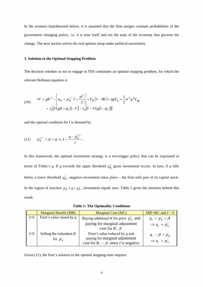
3. Solution to the Optimal Stopping Problem
The decision whether or not to engage in FDI constitutes an optimal stopping problem, for which the
relevant Bellman equation is
(10) ( )
( )( )[ ] ( )( )[ ]2211
222
11
21
2
φλφλ
σηδγ
−−−−++
++−+⎥⎥⎦
⎤
⎢⎢⎣
⎡++−= −+
gVVVgV
VggVKIVIIpagKrV gggKKKa
and the optimal condition for I is denoted by
(11) γ
γ−+
−+ −=⇒=+ K
Kpq
IqIp .
In this framework, the optimal investment strategy is a two-trigger policy that can be expressed in
terms of Tobin´s q. If q exceeds the upper threshold q gross investment occurs. In turn, if q falls
below a lower threshold q , negative investment takes place – the firm sells part of its capital stock.
In the region of inaction , investment equals zero. Table 1 gives the intuition behind this
result.
K+
K−
+− ≤≤ KK pqp
Table 1: The Optimality Conditions
Marginal Benefit (MB) Marginal Cost (MC) MB=MC and I = 0 I>0 Firm’s value raised by q Buying additional K for price and +
Kppaying for marginal adjustment
cost for K: Iγ
Ipq K γ+= ++
++ =⇒ Kpq
I<0 Selling the redundant K for −
KpFirm’s value reduced by q and
paying for marginal adjustment cost for K: Iγ− since I is negative
−− =− KpIq γ
−− =⇒ Kpq
Given (11), the firm´s solution to the optimal stopping time requires
9
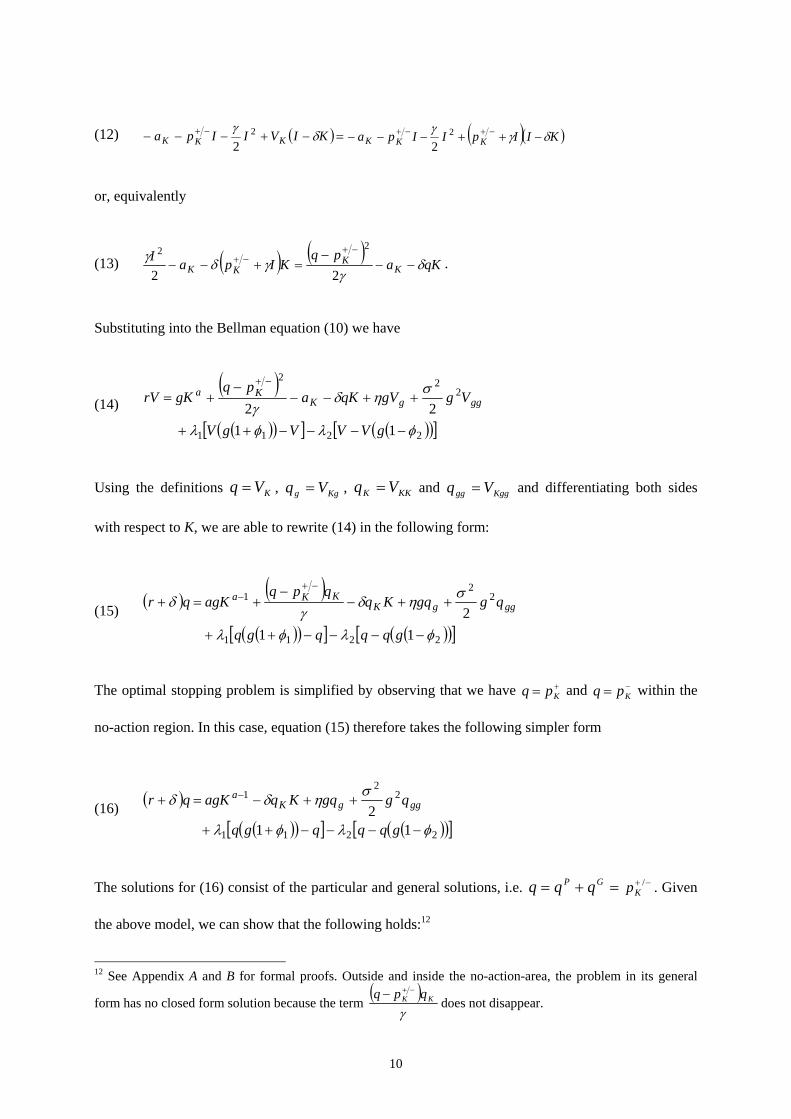
(12) ( ) =−+−−− −+ KIVIIpa KKK δγ 2
2( )( )KIIpIIpa KKK δγ
γ−++−−− −+−+ 2
2
or, equivalently
(13) ( ) ( )qKa
pqKIpaI
KK
KK δγ
γδγ−−
−=+−−
−+−+
22
22.
Substituting into the Bellman equation (10) we have
(14) ( )
( )( )[ ] ( )( )[ ]2211
222
1122
φλφλ
σηδγ
−−−−++
++−−−
+=−+
gVVVgV
VggVqKapq
gKrV gggKKa
Using the definitions KVq = , , Kgg Vq = KKK Vq = and Kgggg Vq = and differentiating both sides
with respect to K, we are able to rewrite (14) in the following form:
(15) ( ) ( )
( )( )[ ] ( )( )[ ]2211
22
1
112
φλφλ
σηδγ
δ
−−−−++
++−−
+=+−+
−
gqqqgq
qggqKqqpq
agKqr gggKKKa
The optimal stopping problem is simplified by observing that we have and within the
no-action region. In this case, equation (15) therefore takes the following simpler form
+= Kpq −= Kpq
(16) ( )
( )( )[ ] ( )( )[ ]2211
22
1
112
φλφλ
σηδδ
−−−−++
++−=+ −
gqqqgq
qggqKqagKqr gggKa
The solutions for (16) consist of the particular and general solutions, i.e. . Given
the above model, we can show that the following holds:
=+= GP qqq −+ /Kp
12
12 See Appendix A and B for formal proofs. Outside and inside the no-action-area, the problem in its general
form has no closed form solution because the term ( )
γKK qpq −+−
does not disappear.
10
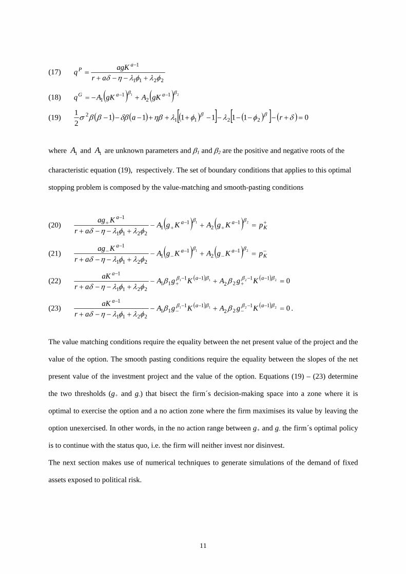
(17) 2211
1
φλφληδ +−−+=
−
aragKq
aP
(18) ( ) ( ) 21 12
11
ββ −− +−= aaG gKAgKAq
(19) ( ) ( ) ( )[ ] ( )[ ] ( ) 011111121
22112 =+−−−−−+++−−− δφλφληβδβββσ ββ ra
where and are unknown parameters and β1A 1A 1 and β2 are the positive and negative roots of the
characteristic equation (19), respectively. The set of boundary conditions that applies to this optimal
stopping problem is composed by the value-matching and smooth-pasting conditions
(20) ( ) ( ) +−+
−+
−+ =+−
+−−+ Kaa
apKgAKgA
arKag 21 1
21
12211
1 ββ
φλφληδ
(21) ( ) ( ) −−−
−−
−− =+−
+−−+ Kaa
apKgAKgA
arKag 21 1
21
12211
1 ββ
φλφληδ
(22) ( ) ( ) 02211 1122
1111
2211
1=+−
+−−+−−
+−−
+
−ββββ ββ
φλφληδaa
aKgAKgA
araK
(23) ( ) ( ) 02211 1122
1111
2211
1=+−
+−−+−−
−−−
−
−ββββ ββ
φλφληδaa
aKgAKgA
araK .
The value matching conditions require the equality between the net present value of the project and the
value of the option. The smooth pasting conditions require the equality between the slopes of the net
present value of the investment project and the value of the option. Equations (19) – (23) determine
the two thresholds (g+ and g-) that bisect the firm´s decision-making space into a zone where it is
optimal to exercise the option and a no action zone where the firm maximises its value by leaving the
option unexercised. In other words, in the no action range between g+ and g- the firm´s optimal policy
is to continue with the status quo, i.e. the firm will neither invest nor disinvest.
The next section makes use of numerical techniques to generate simulations of the demand of fixed
assets exposed to political risk.
11
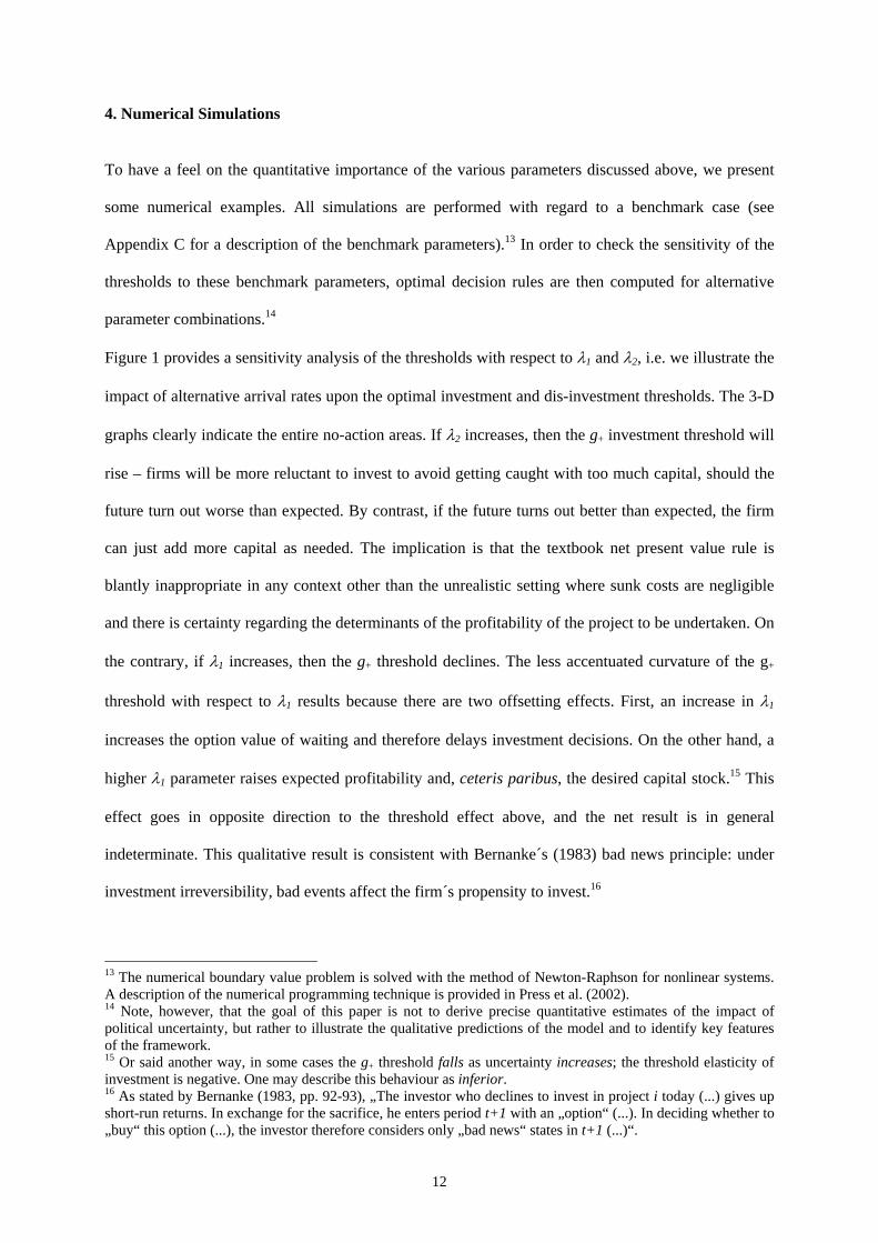
4. Numerical Simulations
To have a feel on the quantitative importance of the various parameters discussed above, we present
some numerical examples. All simulations are performed with regard to a benchmark case (see
Appendix C for a description of the benchmark parameters).13 In order to check the sensitivity of the
thresholds to these benchmark parameters, optimal decision rules are then computed for alternative
parameter combinations.14
Figure 1 provides a sensitivity analysis of the thresholds with respect to λ1 and λ2, i.e. we illustrate the
impact of alternative arrival rates upon the optimal investment and dis-investment thresholds. The 3-D
graphs clearly indicate the entire no-action areas. If λ2 increases, then the g+ investment threshold will
rise – firms will be more reluctant to invest to avoid getting caught with too much capital, should the
future turn out worse than expected. By contrast, if the future turns out better than expected, the firm
can just add more capital as needed. The implication is that the textbook net present value rule is
blantly inappropriate in any context other than the unrealistic setting where sunk costs are negligible
and there is certainty regarding the determinants of the profitability of the project to be undertaken. On
the contrary, if λ1 increases, then the g+ threshold declines. The less accentuated curvature of the g+
threshold with respect to λ1 results because there are two offsetting effects. First, an increase in λ1
increases the option value of waiting and therefore delays investment decisions. On the other hand, a
higher λ1 parameter raises expected profitability and, ceteris paribus, the desired capital stock.15 This
effect goes in opposite direction to the threshold effect above, and the net result is in general
indeterminate. This qualitative result is consistent with Bernanke´s (1983) bad news principle: under
investment irreversibility, bad events affect the firm´s propensity to invest.16
13 The numerical boundary value problem is solved with the method of Newton-Raphson for nonlinear systems. A description of the numerical programming technique is provided in Press et al. (2002). 14 Note, however, that the goal of this paper is not to derive precise quantitative estimates of the impact of political uncertainty, but rather to illustrate the qualitative predictions of the model and to identify key features of the framework. 15 Or said another way, in some cases the g+ threshold falls as uncertainty increases; the threshold elasticity of investment is negative. One may describe this behaviour as inferior. 16 As stated by Bernanke (1983, pp. 92-93), „The investor who declines to invest in project i today (...) gives up short-run returns. In exchange for the sacrifice, he enters period t+1 with an „option“ (...). In deciding whether to „buy“ this option (...), the investor therefore considers only „bad news“ states in t+1 (...)“.
12
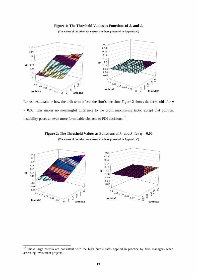
Figure 1: The Threshold Values as Functions of λ1 and λ2
(The values of the other parameters are those presented in Appendix C)
0 0.02 0.
04 0.06 0.
080.
1
00.02
0.040.06
0.080.1
1
1.02
1.04
1.06
1.08
1.1
1.12
1.14
1.16
g+
lambda2lambda1
0 0.02 0.
04 0.06 0.
08 0.1
00.02
0.040.06
0.080.1
00.020.040.060.080.1
0.120.140.160.180.2
g -
lambda2lambda1
Let us next examine how the drift term affects the firm´s decision. Figure 2 shows the thresholds for η
= 0.00. This makes no meaningful difference to the profit maximising tactic except that political
instability poses an even more formidable obstacle to FDI decisions.17
Figure 2: The Threshold Values as Functions of λ1 and λ2 for η = 0.00 (The values of the other parameters are those presented in Appendix C)
0 0.02 0.
04 0.06 0.
080.
1
00.02
0.040.06
0.080.1
1.041.061.081.1
1.121.14
1.16
1.18
1.2
1.22
1.24
g+
lambda2lambda1 0 0.02 0.
04 0.06 0.
08 0.1
00.02
0.040.06
0.080.1
00.020.040.060.080.1
0.120.140.160.180.2
g -
lambda2lambda1
17 These large premia are consistent with the high hurdle rates applied in practice by firm managers when assessing investment projects.
13
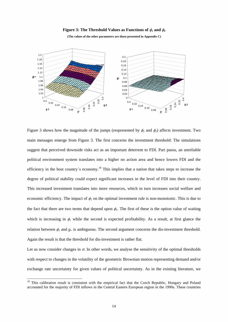
Figure 3: The Threshold Values as Functions of φ1 and φ2
(The values of the other parameters are those presented in Appendix C)
0 0.08 0.
16 0.24 0.
32
0.4
00.08
0.160.24
0.320.4
1
1.021.04
1.06
1.08
1.1
1.12
1.14
1.16
1.18
1.2
g+
φ2
φ1
0 0.08 0.
16 0.24 0.
320.
4
00.08
0.160.24
0.320.4
00.020.040.06
0.080.1
0.12
0.14
0.16
0.18
0.2
g -
φ 2
φ1
Figure 3 shows how the magnitude of the jumps (respresented by φ1 and φ2) affects investment. Two
main messages emerge from Figure 3. The first concerns the investment threshold: The simulations
suggest that perceived downside risks act as an important deterrent to FDI. Pari passu, an unreliable
political environment system translates into a higher no action area and hence lowers FDI and the
efficiency in the host country´s economy.18 This implies that a nation that takes steps to increase the
degree of political stability could expect significant increases in the level of FDI into their country.
This increased investment translates into more resources, which in turn increases social welfare and
economic efficiency. The impact of φ1 on the optimal investment rule is non-monotonic. This is due to
the fact that there are two terms that depend upon φ1. The first of these is the option value of waiting
which is increasing in φ1 while the second is expected profitability. As a result, at first glance the
relation between φ1 and g+ is ambiguous. The second argument concerns the dis-investment threshold.
Again the result is that the threshold for dis-investment is rather flat.
Let us now consider changes in σ. In other words, we analyse the sensitivity of the optimal thresholds
with respect to changes in the volatility of the geometric Brownian motion representing demand and/or
exchange rate uncertainty for given values of political uncertainty. As in the existing literature, we
18 This calibration result is consistent with the empirical fact that the Czech Republic, Hungary and Poland accounted for the majority of FDI inflows in the Central Eastern European region in the 1990s. These countries
14
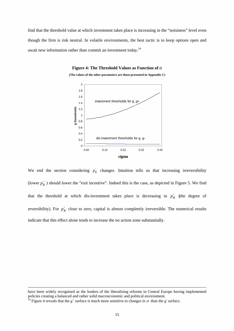
find that the threshold value at which investment takes place is increasing in the “noisiness” level even
though the firm is risk neutral. In volatile environments, the best tactic is to keep options open and
await new information rather than commit an investment today.19
Figure 4: The Threshold Values as Function of σ (The values of the other parameters are those presented in Appendix C)
0
0.2
0.4
0.6
0.8
1
1.2
1.4
1.6
1.8
2
0.02 0.12 0.22 0.32 0.42
sigma
g th
eres
hold
s
investment thresholds for g, g+
dis-investment thresholds for g, g-
We end the section considering changes. Intuition tells us that increasing irreversibility
(lower ) should lower the “exit incentive”. Indeed this is the case, as depicted in Figure 5. We find
that the threshold at which dis-investment takes place is decreasing in (the degree of
reversibility). For close to zero, capital is almost completely irreversible. The numerical results
indicate that this effect alone tends to increase the no action zone substantially.
pK−
pK−
pK−
pK−
have been widely recognised as the leaders of the liberalising reforms in Central Europe having implemented policies creating a balanced and rather solid macroeconomic and political environment. 19 Figure 4 reveals that the g+ surface is much more sensitive to changes in σ than the g- surface.
15
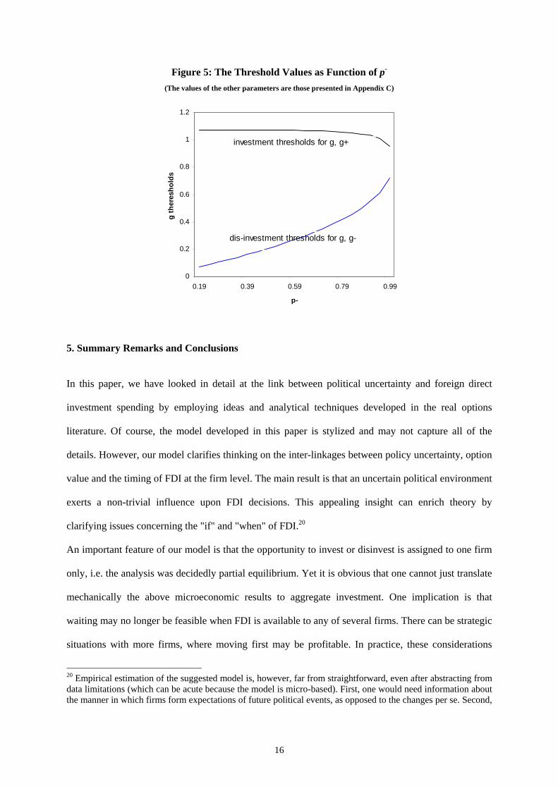
Figure 5: The Threshold Values as Function of p-
(The values of the other parameters are those presented in Appendix C)
0
0.2
0.4
0.6
0.8
1
1.2
0.19 0.39 0.59 0.79 0.99
p-
g th
eres
hold
s
investment thresholds for g, g+
dis-investment thresholds for g, g-
5. Summary Remarks and Conclusions
In this paper, we have looked in detail at the link between political uncertainty and foreign direct
investment spending by employing ideas and analytical techniques developed in the real options
literature. Of course, the model developed in this paper is stylized and may not capture all of the
details. However, our model clarifies thinking on the inter-linkages between policy uncertainty, option
value and the timing of FDI at the firm level. The main result is that an uncertain political environment
exerts a non-trivial influence upon FDI decisions. This appealing insight can enrich theory by
clarifying issues concerning the "if" and "when" of FDI.20
An important feature of our model is that the opportunity to invest or disinvest is assigned to one firm
only, i.e. the analysis was decidedly partial equilibrium. Yet it is obvious that one cannot just translate
mechanically the above microeconomic results to aggregate investment. One implication is that
waiting may no longer be feasible when FDI is available to any of several firms. There can be strategic
situations with more firms, where moving first may be profitable. In practice, these considerations
20 Empirical estimation of the suggested model is, however, far from straightforward, even after abstracting from data limitations (which can be acute because the model is micro-based). First, one would need information about the manner in which firms form expectations of future political events, as opposed to the changes per se. Second,
16
may call for early investment at the same time that political uncertainty suggests waiting. The optimal
choice would then have to balance the two. To assess the role of political uncertainty in aggregate
investment it is also essential to take explicitly into consideration the heterogeneity of individual
firms´ investment decisions. Bertola and Caballero (1994) have explored the implications of
irreversibility for aggregate investment in a model in which individual firms´ investment proceeds in
discontinuous bursts. Individual investments are not synchronized, and firms are subject to
idiosyncratic uncertainty in addition to aggregate uncertainty. As a result, aggregate uncertainty shows
smoothness and a shock may take a long time to develop its full impact. Finally, the discussion
ignored the ability of, and incentives for, firms to diversify their capital stock internationally in times
of political uncertainty. This diversification may partially offset the forces highlighted here.
in reality there are a number of alternative modes to service a foreign market, and failure to consider the entire range of feasible options might lead to a misspecification of the reduced-form empirical equations.
17
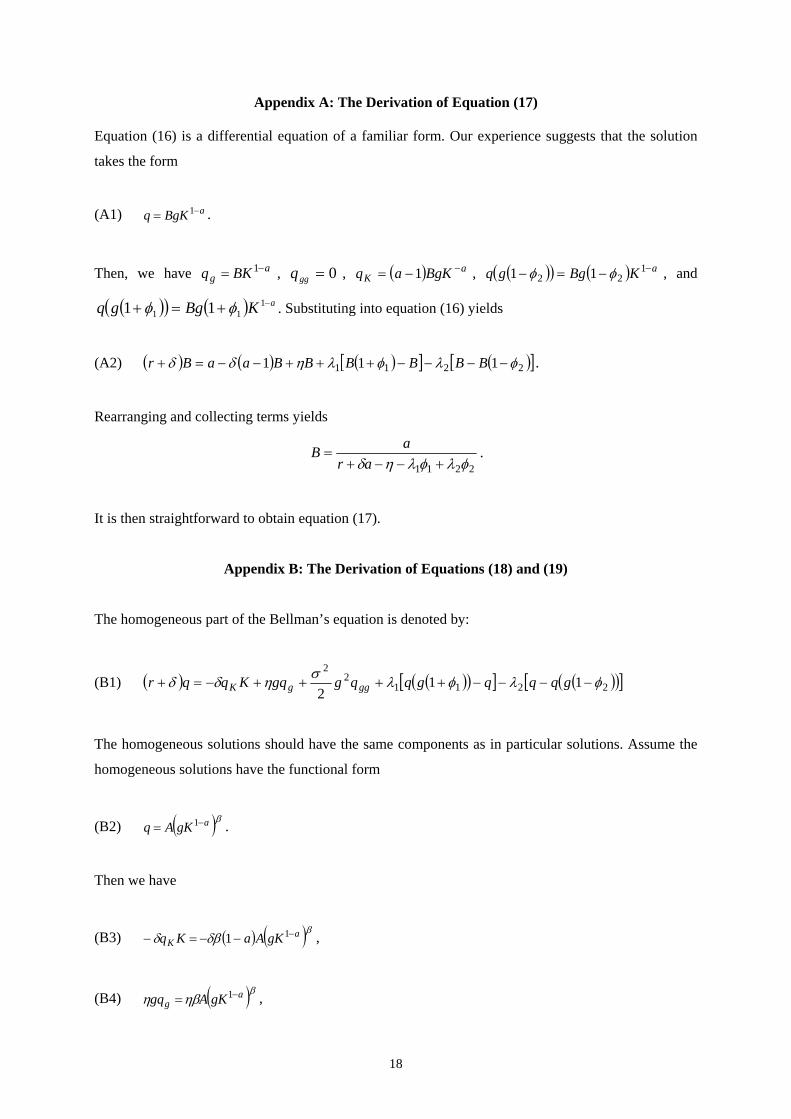
Appendix A: The Derivation of Equation (17) Equation (16) is a differential equation of a familiar form. Our experience suggests that the solution
takes the form
(A1) . aBgKq −= 1
Then, we have , , ag BKq −= 1 0=ggq ( ) a
K BgKaq −−= 1 , ( )( ) ( ) aKBggq −−=− 122 11 φφ , and
. Substituting into equation (16) yields ( )( ) ( ) aKBggq −+=+ 111 11 φφ
(A2) ( ) ( ) ( )[ ] ( )[ ]2211 111 φλφληδδ −−−−+++−−=+ BBBBBBaaBr .
Rearranging and collecting terms yields
2211 φλφληδ +−−+=
araB .
It is then straightforward to obtain equation (17).
Appendix B: The Derivation of Equations (18) and (19)
The homogeneous part of the Bellman’s equation is denoted by:
(B1) ( ) ( )( )[ ] ( )( )[ ]22112
211
2φλφλσηδδ −−−−++++−=+ gqqqgqqggqKqqr gggK
The homogeneous solutions should have the same components as in particular solutions. Assume the
homogeneous solutions have the functional form
(B2) . ( )βagKAq −= 1
Then we have
(B3) , ( ) ( )βδβδ aK gKAaKq −−−=− 11
(B4) , ( )βηβη ag gKAgq −= 1
18
(B5) ( ) ( )βββσσ agg gKAggq −−= 122 1
21
21 ,
(B6) , ( )( ) ( ) ( )ββφφ agKAgq −+=+ 111 11
(B7) . ( )( ) ( ) ( )ββφφ agKAgq −−=− 122 11
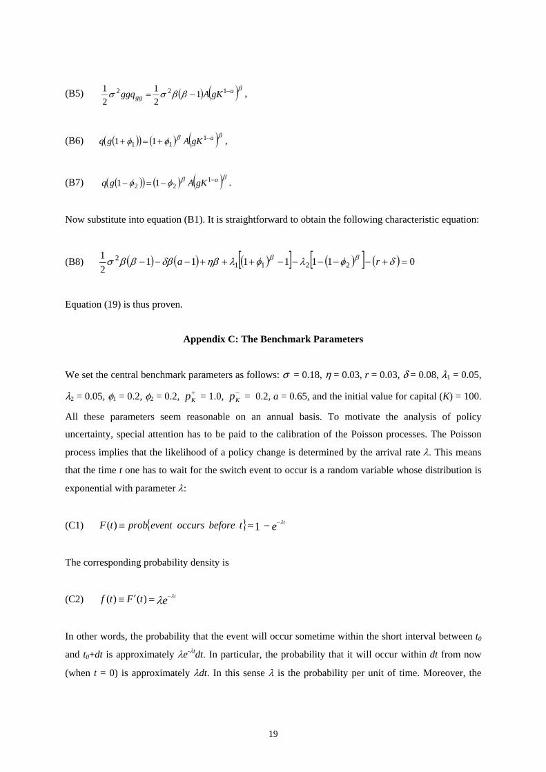
Now substitute into equation (B1). It is straightforward to obtain the following characteristic equation:
(B8) ( ) ( ) ( )[ ] ( )[ ] ( ) 011111121
22112 =+−−−−−+++−−− δφλφληβδβββσ ββ ra
Equation (19) is thus proven.
Appendix C: The Benchmark Parameters
We set the central benchmark parameters as follows: s = 0.18, h = 0.03, r = 0.03, d = 0.08, l1 = 0.05,
l2 = 0.05, f1 = 0.2, f2 = 0.2, = 1.0, = 0.2, a = 0.65, and the initial value for capital (K) = 100.
All these parameters seem reasonable on an annual basis. To motivate the analysis of policy
uncertainty, special attention has to be paid to the calibration of the Poisson processes. The Poisson
process implies that the likelihood of a policy change is determined by the arrival rate λ. This means
that the time t one has to wait for the switch event to occur is a random variable whose distribution is
exponential with parameter λ:
+Kp −
Kp
(C1) { } e ttbeforeoccurseventprobtF λ−−=≡ 1)(
The corresponding probability density is
(C2) e ttFtf λ λ−=′≡ )()(
In other words, the probability that the event will occur sometime within the short interval between t0
and t0+dt is approximately λe-λtdt. In particular, the probability that it will occur within dt from now
(when t = 0) is approximately λdt. In this sense λ is the probability per unit of time. Moreover, the
19
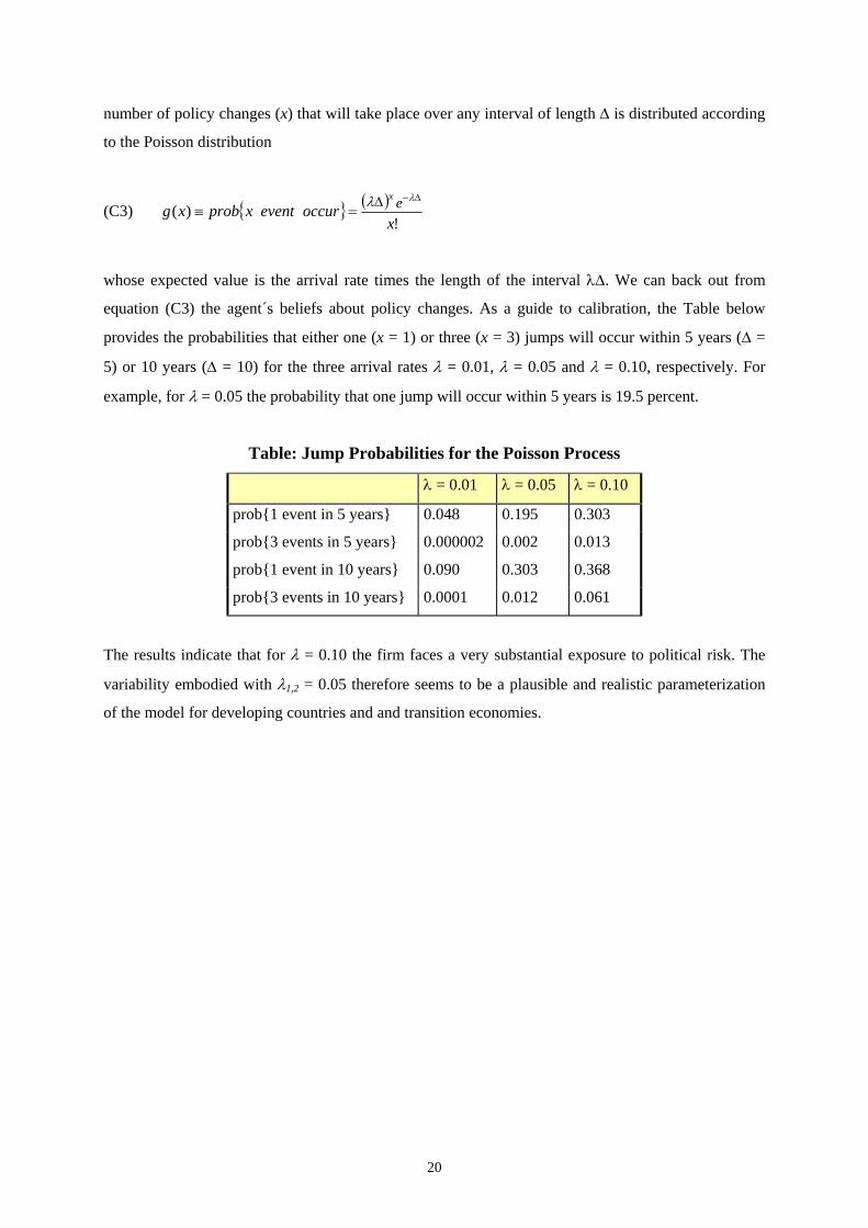
number of policy changes (x) that will take place over any interval of length ∆ is distributed according
to the Poisson distribution
(C3) { } ( )!
)(x
occureventxprobxg ex ∆−∆=≡
λλ
whose expected value is the arrival rate times the length of the interval λ∆. We can back out from
equation (C3) the agent´s beliefs about policy changes. As a guide to calibration, the Table below
provides the probabilities that either one (x = 1) or three (x = 3) jumps will occur within 5 years (∆ =
5) or 10 years (∆ = 10) for the three arrival rates λ = 0.01, λ = 0.05 and λ = 0.10, respectively. For
example, for λ = 0.05 the probability that one jump will occur within 5 years is 19.5 percent.
Table: Jump Probabilities for the Poisson Process
λ = 0.01 λ = 0.05 λ = 0.10
prob{1 event in 5 years} 0.048 0.195 0.303
prob{3 events in 5 years} 0.000002 0.002 0.013
prob{1 event in 10 years} 0.090 0.303 0.368
prob{3 events in 10 years} 0.0001 0.012 0.061
The results indicate that for λ = 0.10 the firm faces a very substantial exposure to political risk. The
variability embodied with λ1,2 = 0.05 therefore seems to be a plausible and realistic parameterization
of the model for developing countries and and transition economies.
20
References:
Abel, A.B., Dixit, A.K., Eberly, J.C. and R.S. Pindyck (1996) “Options, the Value of Capital, and Investment”, Quarterly Journal of Economics 111, 753-777. Abel, A.B. and J.C. Eberly (1994) “A Unified Model of Investment Under Uncertainty”, American Economic Review 84, 1369-1384. Abel, A.B. and J.C. Eberly (1997) “An Exact Solution for the Investment and Value of a Firm Facing Uncertainty, Adjustment Costs, and Irreversibility”, Journal of Economic Dynamics and Control 21, 831-852. Alesina, A. and R. Perotti (1996) “Income Distribution, Political Instability and Investment”, European Economic Review 40, 1203-1228. Amran, M. and N. Kulatilaka (1999) Real Options: Managing Strategic Investment in an Uncertain World, Boston (Harvard Business School Press). Baldwin, R. (1988) „Hysteresis in Import Prices: The Beachhead Effect“, American Economic Review 78, 773-785. Baldwin, R. and P. Krugman (1989) „Persistent Trade Effects of Large Exchange Rate Shocks“, Quarterly Journal of Economics 104, 635-654. Barro, R. (1991) „Economic Growth in a Cross-Section of Countries“, Quarterly Journal of Economics 106, 407-443. Bernanke, B.S. (1983) “Irreversibility, Uncertainty, and Cyclical Investment”, Quarterly Journal of Economics 97, 85-103. Bertola, G. and R.J. Caballero (1994) “Irreversibility and Aggregate Investment”, Review of Economic Studies 61, 223-246. Brenton, P. and D. Gros (1997) “Trade Reorientation and Recovery in Transition Economies”, The Oxford Review of Economic Policy 13, 65-76. Brenton, P. and F. Di Mauro (1999) “The Potential Magnitude and Impact of FDI Flows in CEECs”, Journal of Economic Integration 14, 59-74. Brock, G. (1998) “Foreign Direct Investment in Russia´s Regions 1993-95. Why so Little and where Has It Gone?, Economics of Transition 6, 349-360. Buckley, P. and M. Casson (1981) “The Optimal Timing of a Foreign Direct Investment”, The Economic Journal 91, 75-87. Brunetti, A. and B. Weder (1998) „Investment and Institutional Uncertainty: A Comparative Study of Different Uncertainty Measures“, Weltwirtschaftliches Archiv 134, 513-533. Cherian, J.A. and E. Perotti (2001) „Option Pricing Under Political Risk“, Journal of International Economics 55, 359-377. Copeland, T. and V. Antikarov (2001) Real Options – A Practitioner´s Guide, London (Texere Publishing).
21
Coy, R. (1999) „Exploiting Uncertainty: The Real-Options Revolution in Decision Making“, Business Week, June 7, 118-124. Culem, C. (1988) “The Locational Determinants of Direct Investment Among Industrialized Countries”, European Economic Review 32, 885-904. Dixit, A. and R. Pindyck (1994) Investment Under Uncertainty, Princeton (Princeton University Press). Dunning, J.H. (1993) The Globalisation of Business: The Challenge of the 1990s, London (Routhledge). European Bank for Reconstruction and Development (1994) Transition Report 1994, London. Garibaldi, P., Mora, N., Sahay, R. and J. Zettelmeyer (2002) “What Moves Capital to Transition Economies?”, IMF Working Paper No. 02/64, Washington. Goldberg, L.S. and C.D. Kolstad (1995) “Foreign Direct Investment, Exchange Rate Variability and Demand Uncertainty”, International Economic Review 36, 855-873. Graham, J.R. and C.R. Harvey (2001) “The Theory and Practice of Corporate Finance. Evidence from the Field”, Journal of Financial Economics 60, 187-243. Harrison, J. and D. Kreps (1979) “Martingales and Arbitrage in Multiperiod Securities Markets”, Journal of Economic Theory 20, 381-408. Hassett, K.A. and G.E. Metcalf (1999) „Investment with Uncertain Tax Policy: Does Random Tax Policy Discourage Investment?“, Economic Journal 109, 372-393. Ingersoll, J. and S.A. Ross (1992) “Waiting to Invest: Investment and Uncertainty”, Journal of Business 65, 1-29. Knack, S. And P. Keefer (1995) „Institutions and Economic Performance: Cross-Country Tests Using Alternative Institutional Measures“, Economics and Politics 7, 207-227. Lander, D.M. and G.E. Pinches (1998) “Challenges to the Practical Implementation of Modeling and Valuing Real Options”, Quarterly Review of Economics and Finance 38, 537-567. Markusen, J.R. and K.E. Maskus (2001) “General-Equilibrium Approaches to the Multinational Firm: A Review of Theory and Evidence”, NBER Working Paper No. 8334, Cambridge. Mauro, P. (1995) „Corruption and Growth“, Quarterly Journal of Economics 110, 681-712. McDonald, R. and D. Siegel (1985) “Investment and the Valuation of Firms When There is an Option to Shut Down”, International Economic Review 26, 331-349. McDonald, R. and D. Siegel (1986) “The Value of Waiting to Invest”, Quarterly Journal of Economics 101, 707-727. Pindyck, R.S. and A. Solimano (1993). “Economic Instability and Aggregate Investment”, in: NBER Macroeconomics Annual, Vol. 8, 259-319. Press, W.H., Teukolsky, S.A., Vetterling, W.T. and B.P. Flannery (2002) Numerical Recipes in C++: The Art of Scientific Computing, 2nd edition, Cambridge (Cambridge University Press).
22
Rodrick, D. (1991) „Policy Uncertainty and Private Investment in Developing Countries“, Journal of Development Economics 36, 229-242. Van Wijnbergen, S. (1985) „Trade Reform, Aggregate Investment and Capital Flight“, Economics Letters 19, 369-372.
23