1

Optimum fixed orientations and benefits of tracking for capturing solar

radiation in the continental United States

Matthew Lave and Jan Kleissl Department of Mechanical and Aerospace Engineering

University of California, San Diego Abstract

Optimum tilt and azimuth angles for solar panels were calculated for a grid of 0.1⁰ by 0.1⁰ National Solar Radiation Data Base (NSRDB-SUNY) cells covering the continental United States. The average global irradiation incident on a panel at this optimum orientation over one year was also calculated, and was compared to the solar radiation received by a flat horizontal panel and a 2-axis tracking panel. Optimum tilt and azimuth angles varied by up to 10⁰ from the rule of thumb of latitude tilt and due south azimuth, especially in coastal areas, Florida, Texas, New Mexico, and Colorado. Compared to global horizontal irradiation, irradiation at optimum fixed tilt increased with increasing latitude and by 10% to 25% per year. Irradiation incident on a 2-axis tracking panel in one year was 25% to 45% higher than irradiation received by a panel at optimum fixed orientation. The highest increases in tracking irradiation were seen in the southwestern states, where irradiation was already large, leading to annual irradiation of over 3.4 MWh m-2.

1. Introduction

Solar photovoltaic (PV) systems are quickly gaining popularity in the United States (U.S.), thanks to incentive programs and enhanced interest in environmental sustainability and energy independence. As more PV systems are installed across the U.S., it becomes increasingly important to maximize their power output. Aside from increasing a panel’s solar conversion efficiency, power output can be increased by considering the solar geometry as well as the seasonal and daily variation of atmospheric transmissivity at a particular site. Specifically, it is important to know what the optimum tilt and azimuth angles are at which to mount a fixed tilt panel on a flat roof or on the ground such that it receives maximum irradiation. In addition, knowing the increase in solar radiation incident on a two-axis tracking panel will allow analysis of the economics of tracking PV systems, which are more expensive to install and maintain.

Since the power production of a PV panel is close to linearly proportional to the amount of solar radiation (photons) reaching the panel surface, incident irradiation is an excellent proxy for power output. To maximize absorption of solar radiation in clear skies, the normal to the plane of the PV panel should be pointing towards the sun such that the solar direct beam is perpendicular to the panel surface. While a fixed tilt panel can only be normal to the incident sunlight once a day, a two-axis tracking panel improves over a fixed tilt panel by following the sun through the sky such that the plane of array normal is always parallel to the incident sunlight. However, when the majority of global irradiance is diffuse, horizontal alignment often provides the maximum global irradiance [1].

Some previous studies used modeled extraterrestrial radiation incident on the top of the atmosphere to find equations for optimum tilt over a large area [2,3]. This method accounts for the deterministic (celestial) variables which affect solar radiation, but it does not consider the stochastic (clouds and other weather) variables which also affect the optimum angles. Using an extraterrestrial

2

radiation model, the optimum azimuth is always due south (or north in the southern hemisphere), since solar radiation will be symmetric about solar noon. These studies [2,3] confirmed the simple rule of thumb that tilt angle, 1, equal to latitude, , is optimal for a clear year (e.g., panel at 40⁰N should have

40⁰ tilt from horizontal). For different seasons of the year, the optimum tilt was found to differ by up to 15° from latitude (more in the winter, less in the summer).

Other studies have used measured solar radiation data instead of clear-sky models to account for both the celestial and weather changes. Measured global horizontal irradiation (GHI) at four sites in the U.S. state of Alabama was used to find the optimum yearly tilt angle, [4]. Using a fixed

tilt PV panel at different tilts and a tracking PV panel mounted on a roof in Sanliurfa, Turkey (37⁰ N) optimum tilt and the effect of tracking was quantified [5]. Optimum tilts ranged from 13⁰ in July to 61⁰ in December. Solar irradiation received on a tracking panel was 29% larger compared to a panel at optimum tilt for one day in July. Using measured GHI and diffuse horizontal irradiation (DHI) values the optimum yearly tilt was found to be 3.3⁰ for Brunei Darussalam (4.9⁰ N) [6], and 30.3⁰ for Izmir, Turkey (38.5⁰N) [7].

One comprehensive study computed optimum tilt for a large area using measured irradiation [8]. GHI and DHI from 566 ground meteorological stations across Europe, turbidity data from 611 sites, and a digital elevation model were used to derive expected radiation over a 1 x 1 km grid covering Europe. The optimum yearly panel tilt is less than latitude tilt for Europe and is not solely a function of latitude (as concluded in the clear sky studies), but is also a function of cloudiness.

To the best of our knowledge, maps of optimum tilt and azimuth angles based on measured radiation have not been published for the U.S. In this paper, we present solar maps of the continental United States (CONUS) showing the optimum panel tilt and azimuth, the radiation incident on a panel at optimum tilt and azimuth, and the radiation received by a tracking panel. While maps showing irradiation at latitude tilt facing due south and tracking irradiation have been published by the National Renewable Energy Laboratory (NREL) [9], the NREL maps do not show optimum tilt and azimuth. Furthermore, with their resolution of 40 x 40 km, the maps presented here will have sixteen grid points for every one grid point in the NREL maps. The higher spatial resolution is especially important in areas with strong gradients in radiation, such as coastal or mountainous areas. We will describe the data source (section 2), the model used to compute irradiation on a tilted plane (section 3), and the derivation of optimum angles (section 4). Section 5 presents a validation of the algorithm, and sections 6 and 7 describe the resulting maps and conclusions, respectively.

2. Data

Satellite derived GHI and DHI obtained from the National Solar Radiation Database (NSRDB-SUNY) were used for this study [10]. The NSRDB-SUNY dataset contains hourly GHI, DHI, and direct normal irradiation (DNI) values for the entire United States on a 0.1⁰ node registered grid, corresponding to a grid spacing of about 10 km, for 1998-2005. NSRDB-SUNY was created by applying the model developed at the State University of New York (SUNY) – Albany [11] to satellite imagery of the U.S. from Geostationary Operational Environmental Satellites (GOES). A cloud index was derived for each pixel and was used along with atmospheric turbidity, site elevation, ground snow cover, ground specular reflectance characteristics and individual pixel sun-satellite angle to derive surface irradiations. Atmospheric turbidity is quantified in terms of the air mass independent Linke Turbidity coefficient [12], which is a function of monthly average atmospheric aerosol content, water vapor and ozone. This Linke Turbidity coefficient was used to compute clear sky DNI and DHI. Clear sky DNI was multiplied by a ratio

3

of DNIs calculated using the DIRINT model [13] to find DNI for the actual sky condition. DHI was found by finding the vertical component of DNI [14].

The SUNY gridded data comes from two satellites: GOES-East and GOES-West, which produce snapshot images at 15 minutes past the hour and on the hour, respectively. Although GOES satellite data has a resolution of 1 x 1 km, the data are down-sampled to a 10 km grid to reduce computation time of the SUNY model [14]. For consistency, the SUNY gridded data is shifted and interpolated to model the sum of irradiance incident on each grid point for the previous hour (‘Sglo’ column). This results in each hourly irradiation value having the units of Wh m-2. Hourly uncertainties of the SUNY gridded data range from 8% under optimal conditions to up to 25% [14], though the mean bias error for long periods of time – such as the 8 years used in this study – is expected to be much lower than these values [20].

We chose to use the SUNY gridded data because of the long time period, the high spatial resolution, the consistency in its derivation for a large area, and because DHI and DNI are provided. While the NSRDB and other sources contain measurements from grounds stations which have smaller errors than SUNY measurements, the spatial resolution is poor. The NSRDB, for example, only contains high quality ground irradiation measurements from 221 sites in 40 states [14] as compared to the 97,305 NSRDB-SUNY grid points covering the CONUS.

3. Global Irradiation on a Tilted Plane

3.1 Direct Irradiation

For this study, SUNY irradiations on a horizontal surface had to be converted to irradiations at an arbitrary tilt and azimuth. We chose to use the algorithms described by Page [15] due to the deterministic functional dependence upon location which is desirable in processing data for the entire CONUS. Other models (e.g. Perez et al. [16]) require empirical coefficients which must be determined at each location using ground measurements.

The Page Model takes GHI, DHI, time, latitude, and longitude as inputs and outputs global hourly irradiation (GI) for a panel of any tilt and azimuth as . Direct beam ( ), diffuse

( ), and ground reflected irradiation ( ) on the tilted surface are calculated using astronomical

variables, ground surface albedo, and an empirical function relating diffuse and GI.

Direct (beam) irradiation, , on the tilted surface is a function of tilt and azimuth ( is

due south) as

(1)

where is the solar incidence angle on the tilted panel. is beam normal irradiation at the tilted

panel surface, which is calculated from the SUNY data as

(2)

For computational efficiency, the SUNY DNI was not used , but was found to be similar to from Eq. 2.

and represent GHI and DHI, respectively. The mid-hour solar altitude angle, , is the angular

4

elevation of the sun above the horizontal plane, and is a function of the solar declination angle, the solar hour angle, and the latitude at which the panel is installed. Since the NSRDB-SUNY presents the average of the irradiation over the previous hour, mid-hour values of the solar altitude angle are used since they are nearly an average of the solar altitude angle over the previous hour. For example, the irradiation with time stamp 1100 LST will be the average of irradiation between 1000 LST and 1100 LST and the solar altitude angle will be calculated at 1030 LST.

3.2 Diffuse Irradiation

The diffuse component of irradiation on a tilted surface is significantly more complicated to model. Page [15] computes the ratio of diffuse radiation on the tilted panel to diffuse horizontal radiation as

. (3)

To account for cloud cover, a modulating function in the form of a clearness index, is

used: , where is the correction to the mean solar

distance from earth. We used the empirical function found by Page for Southern Europe to relate

the directionality of diffuse irradiation to the panel tilt angle and clearness index

, (4)

which was accurate for our validation site in Golden, Colorado (see section 5 later).

3.3 Reflected Irradiation

Reflected irradiation, , is modeled by

(5)

where the reflection coefficient is solely a function of panel tilt, . We assumed a ground

surface albedo of as an average for land. Use of albedo maps from remote sensing would be

more accurate, but spatial heterogeneity of albedos within the typical 100 km2 grid cell, especially in urban areas, would still cause a large margin of error. At the orientations used in this study, the sensitivity to albedo is small. In San Diego, California (117.25⁰W, 32.85⁰N), changing the albedo by ±0.1 from the assumed 0.2 leads to a ±0.71% change in the average annual irradiation reaching a panel at optimum orientation and a ±1.08% change for a tracking panel. Similarly, for Albany, New York (73.85⁰W, 42.85⁰N), altering the albedo by ±0.1 leads to a ±0.87% difference for a panel at optimum orientation and a ±1.20% difference in a tracking panel. These albedo changes led to 2° changes in optimum tilt for both San Diego and Albany.

4. Optimum panel angles, tracking, and resulting irradiation 4.1 Optimum tilt and azimuth angles for a fixed panel

5

To determine optimum tilt and azimuth angles, the Page Model was written in function form with inputs of panel tilt, panel azimuth, latitude, longitude, time, , and . The output of this function is the sum

of GI on a panel over the 8 years contained in the SUNY gridded data. Then, for each SUNY grid point (fixed latitude, longitude, time, , and ), the local maximum GI as a function of panel tilt and panel

azimuth was found using unconstrained nonlinear optimization (function ‘fminsearch’ in MATLAB, The Mathworks, Inc.). The optimum tilt and azimuth angle as well as the maximum annual irradiation reaching a panel at optimum fixed tilt were recorded for comparison to horizontal and tracking panels.

4.2 Irradiation onto a Tracking Panel

For concentrating systems, DNI is the relevant metric and corresponding maps already exist [9]. This study focuses on fixed (typically PV) systems and tracking results are only shown for reference. To determine the average annual GI reaching a two axis time-position (or chronological) tracking panel, the same function described in Section 4.1 was used, but the panel tilt angle was set equal to the solar altitude angle while the panel azimuth was set equal to the solar azimuth. While other tracking technologies such as single axis, active or passive tracking exist, we chose to use time-position two-axis tracking due to its simplicity and generality. Other tracking techniques may outperform time-position tracking in high diffuse radiation conditions as then a flat orientation is usually optimal [20].

5. Validation 5.1 Comparison to measurements at SRRL

The model was validated against measured irradiation from the NREL Solar Radiation Research Laboratory (SRRL) located at Golden, Colorado (39.74⁰N, 105.18⁰W). SRRL was selected due to its high data quality and because hourly measurements of GHI, DHI, GI on a surface tilted 40⁰ due south, and GI on a tracking panel all taken at the same location are available. A Kipp and Zonen CM 22 pyranometer measures GHI, another CM 22 pyranometer with a diffuse shading disk measures DHI, an Eppley Laboratory, Inc. Precision Spectral pyranometer measures GI on the tilted surface, and GI for a two axis tracking panel was measured using a Kipp and Zonen CM 21 pyranometer [17].

5.1.1 Tilted Panel

Inputs of hourly GHI and DHI for January 1 to December 31 2009 were obtained from the NREL Measurement and Instrumentation Data Center (MIDC) [ HYPERLINK \l "NRE101" 17 ]. Although 1-minute resolution is available from the MIDC, hourly resolution was chosen to be representative of the hourly SUNY data. We input albedo (0.2), tilt angle (40⁰) and azimuth of the tilted panel (0⁰) to obtain direct, diffuse, and reflected radiation on the tilted surface. These were summed to create an estimated GI on the tilted panel (section 3), which was compared to the measured GI on the tilted panel for times when solar altitude angle > 10⁰ (Fig. 1a).

For this comparison, the mean absolute error (MAE), mean bias error (MBE), root mean squared error (RMSE), relative MBE (rMBE), and relative RMSE (rRMSE) were computed from the instantaneous error, }, by

(6)

6

(7)

(8)

(9)

(10)

(11)

The Pearson correlation coefficient and other error metrics (Table 1) show the strong correlation between the estimated and measured GI. The RMSE for GI on the tilted surface was found to be 5%, which is smaller than errors reported for GHI and DNI in the SUNY-gridded data [14]. Since the 8 year sum is the only value used in creating the maps presented in this paper, the small rMBE value validates the Page Model for our application.

5.1.2 Tracking Panel

The Page Model was also applied for a tracking panel at SRRL, and compared to measured values (Fig. 1b). Again, a high correlation is observed between measured and modeled GI (Table 1). All statistics show larger errors than for the fixed tilt case, but the RMSE (7%) is still smaller than errors reported in the SUNY data [14]. In addition, the rMBE remains very small.

Mean

Measured GI [Wh m-2]

Pearson Correlation Coefficient

[-]

MAE

[Wh m-2]

MBE

[Wh m-2]

RMSE

[Wh m-2]

rMBE

[-]

rRMSE

[-]

40⁰ tilt 541.2 0.997 17.1 2.37 27.5 0.44% 5.0%

tracking 704.4 0.992 29.2 4.84 50.6 0.69% 7.2%

Table 1: Daytime (solar altitude angle>10⁰) statistics for errors between the measured GI at the SRRL panel tilted 40⁰ or the SRRL tracking panel and the calculated GI using the Page Model for 1998-2005.

While the Page Model shows larger MAE and RMSE errors resulting from differences on an hour-by-hour basis, bias errors of GI received on either a fixed tilt or a tracking panel are small. The analysis in this paper relies on 8 year averages of the SUNY-gridded data, so the rMBE is the most important statistic presented in Table 1.

5.2 Comparison to PVWatts

PVWatts2 [18] is a tool published by NREL “to permit non-experts to quickly obtain performance estimates for grid-connected PV systems” [19]. It allows for the calculation of irradiation on a panel of any fixed tilt provided by the user, as well as for a 1- or 2-axis tracking panel at any location in the U.S.

7

using gridded irradiation data at 40 km resolution. Comparisons between PVWatts2 and our algorithm for 5 cities in the U.S. are shown in Table 2. The centers of PVWatts2 grid points do not correspond to the SUNY 10km data, so a distance weighted average of the 4 closest SUNY sites to the center of the PVWatts2 grid point was used to determine the values presented in Table 2. Some deviations between our results and PVWatts2 are expected due to the differences in spatial resolution, especially in areas with large gradients in irradiation. For this reason, the PVWatts2 grid points chosen for Table 2 are far away from coasts, except for Los Angeles, where the grid cells are at least 25 km from the ocean. Overall, the absolute differences between our results and PVWatts2 range from 0.5% to 5.1%. These are smaller than the expected error of PVWatts2 of 10-12% [18], suggesting that our implementation of the Page Model compares well to established models.

Location Optimum Orientation (tilt/azimuth)

GI at Optimum Fixed Orientation [kWh m

-2 day

-1]

GI for Tracking [kWh m

-2 day

-1]

SUNY + Page PVWatts2 rMBE SUNY + Page PVWatts2 rMBE

Orlando, FL (81.35⁰W, 28.49⁰N)

29.1⁰/7.6⁰E 5.22 5.29 -1.3% 6.77 6.81 -0.6%

Dallas, TX (96.84⁰W, 32.72⁰N)

30.5⁰/5.9⁰E 5.09 5.24 -2.9% 6.76 6.92 -2.3%

Phoenix, AZ (112.21⁰W, 33.50⁰N)

33.4⁰/0.3⁰W 6.50 6.29 3.3% 9.09 8.65 5.1%

Los Angeles, CA (-117.95⁰W, 34.08⁰N)

32.4⁰/3.8⁰W 5.79 5.82 -0.5% 7.73 7.52 2.8%

St. Louis, MO (-90.28⁰W, 38.49⁰N)

34.8⁰/1.0⁰W 4.76 4.82 -1.2% 6.25 6.31 1.0%

Table 2: Comparison and relative mean bias error of irradiation calculated from PVWatts2 and Page Model for panels at optimum fixed tilt and for tracking panels at selected sites.

6. Maps

The Page Model was applied to produce solar radiation maps of the CONUS. Figures 2a and 2b show the optimum annual tilt from horizontal and the optimum tilt minus latitude, respectively. The values for optimum tilt were calculated coupled with the optimum azimuth. Since there is an interdependence of optimum azimuth and tilt, optimum tilts at an azimuth of 0⁰ were also calculated, but the mean absolute deviation from Figure 2a was less than 0.1⁰ and the maximum deviation was 1.4⁰. Therefore, results for optimum tilt angels in Figure 2a apply to both optimum azimuth and due south azimuth. Figure 2b can be used to investigate the rule of thumb that panels should be installed at latitude tilt. If latitude tilt were indeed the optimum tilt, then Figure 4 would show zero differences. Indeed, the differences shown in Figure 4 are small for low latitudes, but they become significant at higher latitudes. Some areas exhibit distinct differences in optimum tilt from points at the same latitude, showing that optimum tilt is not solely a function of latitude. Latitude tilt might be accurate for clear sky conditions, but if a site shows seasonal variations in cloudiness, its optimum tilt will be altered. For example, California’s Central Valley experiences Tule fog during winter. Consequently, the optimum tilt there is weighted towards the best tilt in the (clearer) summer months when more radiation can be collected.

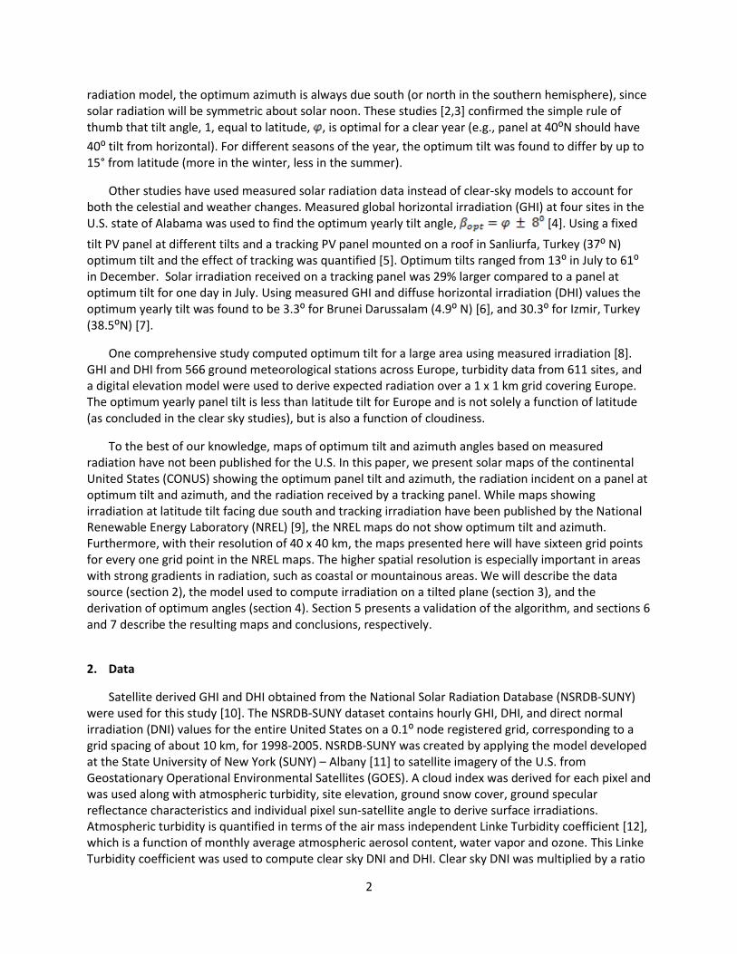
Figure 3 displays the optimum annual azimuth for a solar panel, and can be combined with Figure 2a to determine the optimum annual orientation (tilt and azimuth) for a fixed solar panel. Figure 3 can also be used to investigate whether a due south azimuth results in the maximum irradiation. Due south is optimal for many parts of the country, but there are notable exceptions in Florida, Central Texas, the centers of Wyoming, Colorado, and New Mexico, and along the Pacific Coastline. A due south azimuth

8

would suggest that equal amounts of solar radiation are received before and after solar noon. A non-zero azimuth therefore suggests that solar radiation at a given site was not symmetric. For example, many parts of the Pacific Coastline are subject to summer morning fog that evaporates in the late morning, leading to more afternoon irradiation and thus an optimum azimuth facing towards the west. Large parts of Florida and New Mexico, on the other hand, are often subject to afternoon convective clouds, leading to an optimum azimuth facing east. Figure 3 shows a discontinuity in optimum azimuth angle around a latitude of 107.5o which marks the border between GOES-East and GOES-West satellite data in the SUNY dataset. An error in the time shift of SUNY satellite irradiances to hourly irradiation for the evening hours related to the timing of GOES imagery is the likely explanation [20]. This would indicate that our azimuth angles for the area west of 107.5o are biased towards the west.

The average annual GI reaching a panel at optimum fixed tilt and azimuth is mapped in Figure 4a (a very similar map of irradiation reaching a panel at latitude tilt and south azimuth is presented on the NREL website [9]). This map is useful in determining where it would be best to install fixed solar panels, since incident radiation is nearly linearly proportional to power output of a PV panel. Areas of highest annual solar radiation at optimum tilt are located in the southwestern U.S. including southeastern California, southern Nevada, Arizona, southern Utah, New Mexico, southern Colorado, and western Texas. Most of the rest of the CONUS receives much lower amounts of annual solar radiation at optimum tilt. For example, Florida and the southern tip of Texas are both at lower latitudes than the southwestern states, yet receive around 0.5 MWh m-2 (about 20%) less GI per year.

To determine the importance of installing a solar panel at the optimum orientation, the percentage increase in GI reaching an optimally oriented panel versus GHI is shown in Figure 4b. At almost every location in the CONUS the irradiation increases by at least 10% at optimum orientation over flat. The gain increases with increasing latitude, with a maximum of 25% increase observed in parts of Montana. This is consistent with the increase in optimum tilt shown in Fig. 2a. The further north a site is, the larger the difference between flat and optimum orientation and the larger the increase in irradiation received at optimum orientation.

Figure 5a shows the average annual GI reaching a tracking panel at each location. This map is similar to Fig. 4a which shows the GI at optimum orientation. This is expected since both depend on the GHI reaching each location. However, the solar irradiation reaching tracking panels is significantly larger than the irradiation reaching optimally oriented panels. To quantify this increase, Figure 5b shows the percentage increase in GI reaching a tracking solar panel over a panel at fixed optimal orientation, which ranges from 25% to 45%. The largest percent increases occur in the southwestern U.S., while the smallest increases occur in the eastern U.S. and on the Pacific Coastline. The large increases are related to clear skies when irradiance is more variable as a function of view angle and tracking shows greater benefits. Smaller increases are related to cloudy conditions which cause more uniform diffuse irradiation patterns. In cloudy conditions other tracking strategies would result in a slightly better performance (section 4.2). The highest percentage increases occur in areas where irradiation at optimum tilt was already large (i.e., less cloudy areas), making tracking panels very attractive for areas such as the southwestern states.

7 Conclusion

The optimum tilt and azimuth angles to collect global solar irradiation (GI) in the CONUS were determined using the Page Model applied to the SUNY 10 km gridded data. While rules of thumb suggest that maximum GI is obtained at latitude tilt with an azimuth facing due south, it was found for

9

most locations in the CONUS that higher GI could be obtained by deviating from this rule. The optimum tilt was never found to be greater than latitude tilt, but it was found to be up to 10⁰ less than latitude tilt. On average, the deviation from latitude tilt increased at higher latitudes, but optimum tilt was not found to simply be a function of latitude. Seasonal weather patterns such as winter clouds led to changes in the optimum tilt. Azimuths deviating up to 10⁰ west or east of due south were found for areas with typical daily cloud patterns such as morning fog or afternoon thunderstorms.

Areas of high GI on an optimal fixed orientation panel occur in the southwestern U.S., with up to 2.4 MWh m-2 per year. Compared to global horizontal irradiation, irradiation at optimum fixed tilt increased with increasing latitude and by 10% to 25% per year. These increases are significant considering they require no more active work than determining the optimum orientation during panel installation. However, the sensitivity of annual irradiation to inclination is small near the optimum point. While small increases in power production may have a significant impact on economic payback time, other factors such as aesthetics and mounting considerations may dictate a near-optimal angle that would result in a relatively small loss in annual power production.

GI reaching a tracking surface shows very similar geographic patterns to GI at optimum fixed orientation, but a tracking panel can receive over 3.4 MWh m-2 per year. The increase from using a tracking panel was strongest where fixed orientation irradiation was large, corresponding to relatively clear skies on average. This suggests using tracking panels in areas of high irradiation so long as the increases are enough to balance the higher initial costs, maintenance costs, and energy lost to the tracking mechanism.

Overall, we found that the rule of thumb for orientation of a solar panel was up to 10⁰ off for tilt, azimuth, or both. We recommend using optimum tilt and azimuth angles presented here to increase irradiation received at any site. Our analysis does not consider the temperature effect on PV efficiency. Given that the panel temperatures are larger in summer than in winter and larger in the afternoon than in the morning, consideration of this effect would result in larger tilts and an azimuth facing more east of south, but the changes are expected to be small and depend on the PV temperature coefficient. Moreover this analysis optimizes for annual irradiation, but does not consider the seasonality and diurnal pattern of electricity prices. If the PV array output displaces consumption from the local facility with time-of-use pricing or if the electricity generated is bid into the market, the irradiations would have to be weighted by the electricity price at the time to determine economic effects. Since electricity prices vary by region and time, accumulating such a database from 1997-2005 was beyond the scope of this project. Generally, since electricity is more expensive in the summer and during the afternoon peak demand the optimum azimuth would be further west of south and the optimum tilt would be closer to zero if economic consideration were taken into account.

Acknowledgements

We appreciate funding from the DOE High Solar PV Penetration grant 10DE-EE002055. The maps presented in this paper are also available as supplementary material for use with Google Earth.

10

1. 20. Kelly, N.A., T.L. Gibson, ‘Improved photovoltaic energy output for cloudy conditions with a solar tracking system’, Solar Energy 83 (2009) 2092–2102

2. J.A. Duffie, W.A. Beckman, Solar Engineering of Thermal Processes, Wiley, New York, 1980, pp. 90-101.

3. H.P. Garg, Treatise on Solar Energy: Volume1: Fundamentals of Solar Energy, Wiley, New York, 1982, pp. 375-381.

4. G. Lewis, Optimum tilt of a solar collector, Solar & Wind Technology. 4 (1987) 407-410.

5. M. Kacira, M. Simsek, Y. Babur, S. Demirkol, Determining optimum tilt angles and orientations of photovoltaic panels in Sanliurfa, Turkey, Renewable Energy. 29 (2004) 1265-1275.

6. M.A.M.Yakup, A.Q. Malik, Optimum tilt angle and orientation for solar collector in Brunei Darussalam, Renewable Energy. 24 (2001) 223-234.

7. K. Ulgen, Optimum tilt angle for solar collectors, Energy Sources. 28 (2006) 1171-1180.

8. M. Suri, T.A. Huld, E.D. Dunlop, PV-GIS: a web-based solar radiation database for the calculation of PV potential in Europe, Int. J. of Sustainable Energy. 24 (2005) 55-67.

9. NREL, Dynamic maps, GIS data, and analysis tools - solar maps, <http://www.nrel.gov/gis/solar.html>. Accessed May 7, 2010.

10. NREL, National Solar Radiation Database, 1991-2005 Update. <http://rredc.nrel.gov/solar/old_data/nsrdb/1991-2005/>. Accessed May 7, 2010.

11. R. Perez, P. Ineichen, K. Moore, M. Kmiecik, C. Chain, R. George, F. Vignola, A new operational model for satellite-derieved irradiances: descritpion and verification, Solar Energy.73 (2002) 307-317.

12. P. Ineichen, R. Perez, A new airmass independent formulation for the Linke turbidity coefficent, Solar Energy. 73 (2002) 151-157.

13. R. Perez, P. Ineichen, E. Maxwell, R. Seals, A. Zelenka, Dynamic Global-to-Direct Irradiance Conversion Models, ASHRAE Transactions-Research Series, 1992, pp. 354-369.

14. S. Wilcox, National solar radiation database 1991-2005 update: user's manual, 2007, NREL/TP-581-41364.

15. J. Page, The Role of Solar Radiation Climatology in the Design of Photovoltaic Systems, in: T. Markvart, L. Castaner, Practical Handbook of Photovoltaics: Fundamentals and Applications, Elsevier, Oxford, 2003, pp. 5-66.

16. R. Perez, R. Stewart, C. Arbogast, R. Seals, J. Scott, An anisotropic hourly diffuse radiation model

11

for sloping surfaces: description, performance validation, site dependency errors, Solar Energy. 36 (1986) 481-498.

17. NREL, Measurement and Instrumentation Data Center (MIDC), <http://www.nrel.gov/midc/>. Accessed May 7, 2010.

18. B. Marion, M. Anderberg, R. George, P. Gray-Hann, D. Heimiller, PVWATTS version 2 - enhanced spatial resolution for calculating grid-connected PV-performance, 2001, NREL/CP-560-30941.

19. NREL, PVWatts: a performance calculator for grid-connected PV systems, version 2. <http://rredc.nrel.gov/solar/calculators/PVWATTS/versions2/>. Accessed May 7, 2010.

19. Nottrott, A., J. Kleissl, Validation of the SUNY NSRDB global horizontal irradiance in California, Solar Energy, in press

12

0 200 400 600 800 1000 12000

200

400

600

800

1000

1200

measured GI on tilted panel [W m-2

]

estim

ate

d G

I usin

g P

age M

odel [W

m-2

]

a.

0 200 400 600 800 1000 12000

200

400

600

800

1000

1200

measured GI on tracking panel [W m-2

]

estim

ate

d G

I usin

g P

age M

odel [W

m-2

]

b.

Figure 1: Scatter plot of (a) the measured GI on a surface at 40⁰ tilt, facing due south, and (b) the

measured GI on a tracking panel, plotted versus values calculated using the Page Model. Measurements

were taken at SRRL in Golden, Colorado. The values shown are hourly daytime values (solar elevation

angle >10⁰) for the entire year 2009. The solid lines are 1:1 lines for reference.

13

Figure 2a: Map of the optimum tilt from horizontal to maximize annual incident GI.

Figure 2b: Map of the optimum tilt from horizontal (Fig. 2a) minus the latitude for each location. This

shows the difference in degrees between the optimum tilt and the rule of thumb suggesting latitude tilt.

14

Figure 3: Map showing the optimum azimuth to maximize incident GI. Due south is 0⁰, and values shown

on the map are east or west of due south. When coupled with Figure 2a, the optimum orientation (tilt

and azimuth) at any location on the map can be determined.

15

Figure 4a: Map showing the average annual GI reaching a panel at optimum tilt and azimuth.

Figure 4b: Map showing the percentage increase in GI incident on a PV panel at optimum tilt and

azimuth versus a flat horizontal panel.

16

Figure 5a: Map of the annual GI reaching a two-axis tracking solar panel.

Figure 5b: Map of the percentage increase in GI reaching a tracking panel over GI reaching a panel at

fixed optimum orientation.