optimum blood sampling time windows for parameter estimation in population pharmacokinetic...

STATISTICS IN MEDICINEStatist. Med. 2006; 25:4004–4019Published online 3 February 2006 in Wiley InterScience (www.interscience.wiley.com). DOI: 10.1002/sim.2512

Optimum blood sampling time windows for parameterestimation in population pharmacokinetic experiments

Gordon Graham1;∗;† and Leon Aarons2;‡

1Novartis Pharma AG, Lichtstrasse 35, CH-4056 Basel, Switzerland2School of Pharmacy and Pharmaceutical Sciences; University of Manchester; Oxford Road;

Manchester M13 9PL; U.K.

SUMMARY

Clinical trials requiring the collection of pharmacokinetic information often specify blood samples tobe taken at �xed times. This may be feasible when trial participants are in a controlled environmentsuch as in early phase clinical trials, however it becomes problematic in trials where patients are in anout-patient clinic setting such as in late phase drug development. In such a situation it is common totake blood samples when it is convenient for all involved and may result in data that are uninformative.This paper proposes an approach to pharmacokinetic study design that allows greater �exibility as towhen blood samples can be taken and still result in data that allows satisfactory parameter estimation.The sampling window approach proposed in this paper is based on determining time intervals around theD-optimum pharmacokinetic sampling times. These intervals are determined by allowing the samplingwindow design to result in a speci�ed level of e�ciency when compared to the �xed times D-optimumdesign. Several approaches are suggested for dealing with this design problem. Copyright ? 2006 JohnWiley & Sons, Ltd.

KEY WORDS: optimum experimental design; pharmacokinetics; mixed e�ects models; D-optimality;sampling windows; e�ciency

1. INTRODUCTION

To determine the pharmacokinetics of a drug, �uid samples (usually blood) are collected overtime. This is generally the case whether in a preclinical setting such as for toxicokinetic

∗Correspondence to: G. Graham, Novartis Pharma AG, Lichtstrasse 35, CH-4056 Basel, Switzerland.†E-mail: [email protected]‡E-mail: [email protected]

Contract=grant sponsor: GlaxosmithklineContract=grant sponsor: P�zerContract=grant sponsor: NovartisContract=grant sponsor: LillyContract=grant sponsor: Servier

Received 2 August 2005Copyright ? 2006 John Wiley & Sons, Ltd. Accepted 21 December 2005

OPTIMUM SAMPLING WINDOWS FOR PHARMACOKINETIC EXPERIMENTS 4005

experiments [1] or a clinical setting involving healthy subjects or patients. A considerableamount of work has been reported previously on the application of non-linear mixed e�ectsmodels to pharmacokinetic data (referred to as population pharmacokinetics in the pharmaco-logical literature) [2–4]. Population pharmacokinetic models characterize the mean pharma-cokinetic time-course of a compound and quantify the inter-subject and residual (intra-subject)variability. Additionally, patient speci�c covariates such as demographic, environmental andhealth status variables can be incorporated to describe the variability in the clinically relevantmodel parameters [5, 6]. The design of a pharmacokinetic study resulting in the data collectionand analysis outlined above involves the setting of many design variables. These primarilyinclude the number of subjects, the number of blood samples per subject and the times atwhich blood samples are collected. In addition there could be subpopulations that have alteredpharmacokinetics from the ‘normal’ population and may require alternative designs. Moreoverit may be necessary to balance the study for the covariate e�ects, although this is rarely done.Given the scope of variables involved, it is apparent that the design of such experiments forcharacterizing the pharmacokinetics in a population is complex.In the pharmacokinetic literature, there has been some e�ort to explore better designs for

such experiments by using modelling and simulation [7–10]. Recently, optimum experimen-tal design methodology has gained greater exposure in pharmacokinetics, although it hasbeen discussed intermittently over the last 25 years. Optimum design for �xed e�ects mod-els (or single individuals in pharmacokinetic studies) have been considered in terms of localdesigns [11–15] and Bayesian D-optimum designs [16]. Mentr�e et al. [17, 18] were the �rstto apply D-optimum design to random e�ects models in the area of toxicokinetics, with subse-quent application of this methodology to population pharmacokinetics and pharmacodynamics[19–21].In a phase III clinical trial, taking blood samples at exact times is di�cult to accomplish

as the patients are in an uncontrolled environment. Patients arrive at an out-patient clinicand have samples taken whenever it is possible to do so. This could be because there aredelays in seeing the medical personnel, the patient may have taken the drug before arrivingat the clinic so an exact time of dosing is not known or more immediate medical proceduresmay make sample collection di�cult. This makes the resulting data observational in natureand is a less informative approach to characterizing the pharmacokinetics in the populationof interest. Also, characterizing the pharmacokinetics in a phase III trial is often at best asecondary objective and if blood samples are taken, there is a desire to make the collectionof these samples as �exible as possible.A sampling window approach (blood samples taken in speci�ed time intervals) has pre-

viously been used in practice as an attempt at controlling the blood sampling times yetallowing some �exibility in when the samples can be taken due to logistical constraints.Sampling windows have been proposed because of the �exibility they o�er in performingthe trial while still resulting in informative data. Aarons et al. [22] reported that samplingwindow designs have been widely used but without presenting any details of how they arede�ned. Jonsson et al. [23] considered the problem of pharmacokinetic parameter estima-tion in a phase III clinical trial where patients visited a clinic to have blood samples takeneither during a morning or afternoon session. Hashimoto and Sheiner [24] showed that dis-crete random sampling times did not adversely a�ect the parameter estimates of a populationpharmacokinetic–pharmacodynamic model. Du�ull et al. [20] and Green and Du�ull [25]determined ‘conditional’ sampling windows for a population pharmacodynamic model and

Copyright ? 2006 John Wiley & Sons, Ltd. Statist. Med. 2006; 25:4004–4019

4006 G. GRAHAM AND L. AARONS

population pharmacokinetic model, respectively, by taking the population D-optimum designand varying one time point at a time until the normalized determinant of the Fisher infor-mation matrix was reduced by 5 per cent. This means that one does not prospectively assessthe joint loss of e�ciency in the sampling window design when compared to the D-optimumdesign. The approach adopted by Pronzato [26] is closest to the method proposed in thisarticle. Pronzato [26] presents results for when the sampling windows can be determined an-alytically for �xed e�ects models. In the case of Pronzato [26], the window length is �xed insome prespeci�ed way and the aim is to determine where the windows should be positioned.This paper presents an alternative approach to optimizing pharmacokinetic sampling window

designs where the joint sampling windows attain a speci�ed level of e�ciency when comparedto the �xed times D-optimum design. D-e�ciency corresponds to the normalized determinantof the Fisher information matrix for the sampling window design divided by the normalizeddeterminant of the Fisher information matrix for the D-optimum design of the pharmacokineticmodel in question.An outline of this paper is as follows. Section 2 speci�es the non-linear mixed e�ects model

that will be investigated and Section 3 highlights the derivation of the Fisher informationmatrix for this model. Section 4 develops the ideas for obtaining an optimum blood samplingwindow design for population pharmacokinetic studies. Sections 5 and 6 present applicationsof the approach for an example taken from the literature and a simulation study, respectively.Finally, a discussion and some concluding remarks are given.

2. THE PHARMACOKINETIC MIXED EFFECTS MODEL

The pharmacokinetic mixed e�ects model can be speci�ed as a two stage hierarchical model(assuming normality).Stage 1: Individual Level (conditional likelihood)

yij=f(�i; tij) + ”ij; i=1; : : : ; N and j=1; : : : ; ni

Yij | bi ∼N (f(�i; tij); �2)

Stage 2: Population Level (random e�ects distribution assuming normality)

�i=�+ bi; i=1; : : : ; N

bi∼N (0;�)

where i indexes the individual and j indexes the repeated measurements within an individual,N is the number of subjects, ni is the number of repeated measurements for subject i, yij andYij are the observed and random response variable, tij is the design variable, �i is the p× 1vector of parameters for individual i, f is the pharmacokinetic model, �ij is the residual error,bi is the p× 1 vector of individual deviations from the population mean �, � is the intersubjectvariance matrix and �2 is the residual variance. Dosage regimen is assumed known in thispaper, and tij corresponds to blood sampling times only. The intersubject variance–covariancematrix is assumed to be diagonal so that �=diag(!21; : : : ; !

2p). The marginal likelihood is



obtained by integrating the conditional likelihood over the random e�ects distributions as

L(�;�; �2;y)=N∏i=1

∫ ni∏j=1

N(f(�i; tij); �2)N(0;�)dbi

where y=(yT1 ; : : : ; yTN )T, and yi=(yi1; : : : ; yini)

T. From now on the parameter set (�;�; �2) isdenoted by �.

3. FISHER INFORMATION MATRIX

To determine the optimum design, we need to specify �rstly a method for calculating theFisher information matrix for the population pharmacokinetic model parameters. To do thiswe need to evaluate the integral above for the marginal likelihood, L(�;y). For non-linearmodels this is analytically intractable and approximations such as Gauss–Hermite quadrature,linearization or Monte Carlo methods have been used. Linearization of the model aroundbi=0 has been used predominantly in population pharmacokinetics optimum design [17–21]and is used here. The marginal likelihood for a single subject after linearization is given byYi ∼N(f(�; �i); Vi) where, �i=(ti1; : : : ; tini)T, Vi= Ji�J Ti +�i, Ji= @fT(�; �i)=@� is the p× niJacobian matrix for the ith individual evaluated at individual i’s design points and �i=�2Ini isthe residual variance matrix for subject i. The Fisher information matrix for a single individualis given by

M (�; �i)≈[J Ti V

−1i Ji 0

0 2−1Fi

]

where

Fi= − 2E(@l(�;�;�i;yi)

@�r@�s

)= tr

(V−1i@Vi@�r

V−1i@Vi@�s

)

�=[!21; : : : ; !2p; �

2]T, l is the log-likelihood, and r; s=1; : : : ; p+ 1 (number of variance com-ponents) (see Reference [27] for a detailed description). The information matrix for the Nsubjects is given by

∑Ni=1M (�; �i).

4. OPTIMAL SAMPLING WINDOW DESIGN

Each element of the design vector for individual i, �i=(ti1; : : : ; tini)T, remains to be chosen

from the design space, A=[a0; b0], where a0 and b0 are the lower and upper time limitsbetween which blood samples can be taken. It is assumed here that the D-optimum crite-rion is the reference criterion, and let the D-optimum design for individual i be denoted�Di =(t

Di1; : : : ; t

Dini)

T. It is also assumed that all subjects have the same number of blood samples(ni= n) planned at the same times, and so the subscript i is dropped from the notation unlessexplicitly required. The information matrix for the population pharmacokinetic model can thenbe written as M (�;�), where �= (�1; : : : ; �N ) is the population design and �i= �=(t1; : : : ; tn)for i=1; : : : ; N .



Assume that instead of taking observations at the exact time points, �D, we specify intervalsaround the D-optimum design points from which we take blood samples. For example, if thereare 3 distinct D-optimum time points then we can specify 3 time intervals around the optimumtime points. Each subject recruited to have blood samples taken will have one sample drawnfrom each of these 3 sampling windows. This results in each subject having their own setof 3 blood sampling times. For example, if the times at which blood samples can be drawnare uniformly distributed within the sampling windows, then for subject i, the sampling timesare distributed as tij ∼U(aj; bj) for j=1; 2; 3. This is repeated for all N subjects, which willgenerate a distribution (uniform in this example) of blood sampling times within each samplingwindow. The realized sampling times for individual i are then denoted si=(si1; : : : ; sin) andthe realized population design is denoted S=(s1; : : : ; sN ).Let the intervals around each distinct D-optimum design point, tDj , be denoted by [aj; bj],

where aj¡bj, a06a1¡ · · ·¡an¡b0 and a0¡b1¡ · · ·¡bn6b0. As a �rst case let each interval[aj; bj] have length 2� such that aj= tDj −� and bj= tDj +� for j=1; : : : ; n and �¿0, and thatrandomly sampled times are uniformly distributed, with care being taken so that the samplingwindows do not extend outside the design space. The sampling window design can thenbe speci�ed as �W =(tW1 ; : : : ; t

Wn ) where t

Wj is a random time from the uniform distribution

U�(aj; bj). This speci�cation means that it is possible for the sampling intervals to overlap,e.g. aj¡bj−1. This can be a problem because if a blood sample is taken at time sj from thesampling window [aj; bj] and sj¿aj+1, then in clinical practice it is impossible to take thenext sample at any time in the interval [aj+1; sj] from the window [aj+1; bj+1]. It is thereforedesirable to have non-overlapping sampling windows. However under the model and designconstraints considered in the examples presented later, this problem does not arise. Of course,this might happen using di�erent design criteria and constraints, and would require the designoptimization algorithm to be constrained accordingly.One way to construct a sampling window design is to allow for a speci�ed loss of e�ciency

compared to the D-optimum design and relate �, a univariate parameter representing thelength of the design windows, to the e�ciency loss. This means that a univariate parameteris optimized to determine the length of the sampling windows around �D. The D-e�ciencyis given by

e�D(�)=( |M (�;�)|

|M (�;�D)|)1=(2p+1)

where the power (2p+ 1)−1 is the normalizing term corresponding to the reciprocal numberof parameters to be estimated in the population pharmacokinetic model described in Sec-tion 2. The mean e�ciency of a sampling window design, �W =(�W1 ; : : : ; �

WN ) with �

Wi = �

W

for all i and tWj ∼U�(aj; bj) for all j, is then given by

e�D(�W )=E[|M (�;�W )|1=(2p+1)]

|M (�;�D)|1=(2p+1)

where E[·] is the expectation of the normalized determinant of the Fisher information matrixover the distribution of sampling times. M (�;�W ) cannot be calculated because �W is a set ofsampling time distributions but M (�; SW ) can be evaluated. However, the expected normalized



determinant of the information matrix for the sampling window design can be calculated as

E[|M (�;�W )|1=(2p+1)]=∫ bn

an· · ·∫ b1

a1|M (�; SW )|1=(2p+1)U�(a1; b1) : : : U�(an; bn) dsW1 · · · dsWn

where, as stated previously, aj= tDj − � and bj = tDj + � for j=1; : : : ; nIf the aim is to achieve a mean e�ciency of e�0 for the sampling window design compared

to the D-optimum design, one approach to calculating the optimum window length parameter,�W , is to minimize the quadratic loss function

�W = argmin�[(e�D(�W )− e�0)2]

If the integral for the normalized determinant of the information matrix can be calculatedanalytically then the calculation of �W is straightforward. If this is not possible, which islikely to be the case in most pharmacokinetic situations, then we can evaluate the integral byMonte Carlo sampling as

E[|M (�;�W )|1=(2p+1)]≈ 1H

H∑h=1

∣∣∣∣ N∑i=1M (�; sW (h)i )

∣∣∣∣1=(2p+1)

where H is the number of sampled population designs, sW (h)i =(sW (h)i1 ; : : : ; sW (h)in )T is the hthsimulated vector of n design points for individual i and sW (h)ij is a sampled design pointfrom the jth sampling window U�(aj; bj). Throughout this paper, 200 Monte Carlo samples(population designs) will be used at each iteration when optimizing the sampling windowparameter, �.The normalized determinant of the information matrix for the sampling window design

could have been de�ned di�erently, for example as

(∫ bn

an· · ·∫ b1

a1|M (�; SW )|U�(a1; b1) : : : U�(an; bn)dsW1 · · · dsWn

)1=(2p+1)

where the normalization is performed after the integration. Although this does have an im-pact on the results of the optimized sampling window designs, the di�erences are smallfor the examples considered in this paper, so this criterion is not considered anyfurther.The criterion above requires the mean e�ciency of the realized population designs to equal

e�0. This design can then be termed the mean e�ciency sampling window design. How-ever, each time the sampling window design is implemented a random set of sampling timeswill result and a distribution of population designs is obtained. One of the problems thatwill result from such an approach is that the variation in the realized designs will causethe observed D-e�ciency to be smaller than the mean e�ciency on occasions. Higher D-e�ciencies are less likely to be a problem (e.g. if the design points are close to the D-optimumtime points) than lower D-e�ciencies where, for example, all blood sampling times are ‘far’from the D-optimum times. We approximate the speci�ed sampling window distributions ina given study by the empirical distribution of the randomly sampled times of each individual.



If the number of patients, N , is small then the empirical distribution will approximate the truedistribution less well than if N was large. The mean e�ciency for the sampled populationdesign compared to the D-optimum design will on average be the same as the true meane�ciency regardless of the sample size. However, the uncertainty in the mean e�ciency willbe larger with smaller N . It is then useful to de�ne a probability interval around the expectede�ciency to assess the uncertainty in the e�ciency as a function of the number of subjectsincluded in the study.Alternatively to requiring the mean e�ciency be e�0, we could require that 100×(1 − )

per cent of all observed (simulated) population designs be no less than e�0 D-e�cient. Forexample we may want the lower bound of the 90 per cent one sided probability interval onthe sampling window e�ciency for a given number of blood samples and subjects be at least95 per cent D-e�cient. This sampling window criterion can be de�ned as

e� D(�W )= {Pr(e�D(M (�; SW ))¿e�0)¿1− }

where is the lower tail percentile. The optimum window length parameter, �W , is found byincluding the above criterion in the quadratic loss function and minimizing over � as

�W =argmin�[(e� D(�

W )− e�0)2]

To evaluate the probability of a given sampling window design being at least e�0 D-e�cient,sample H population designs Sh=(sh1; : : : ; s

hn) from �W as described earlier. Evaluate the

e�ciency of each Sh compared to �D. The probability of the sampling window design givinga D-e�ciency less than e�0 is the proportion of sampled population designs with an e�ciencyless than e�0.The probability interval for the e�ciency could also be re-expressed as a probability interval

for the window length, �.

4.1. Sampling window distributions

So far each sampling window has been assumed to be uniformly distributed. This may notbe appropriate in all situations. It may not be optimum either as an alternative samplingdistribution may re�ect the blood sampling observed in clinical practice more accurately.We can in general de�ne a design variable density function, g�(sW ; ) which is de�ned onthe domain of the sampling windows as a function of � and possibly other parameters, .Assuming there are n distinct D-optimum design points and a sampling window around eachtime point, two examples of design variable density functions in addition to the uniformdistribution described previously are:Log-Uniform

g�(sW ; )=

⎧⎪⎪⎨⎪⎪⎩

s−1jlog(bj)− log(aj) ; aj¡sj¡bj; j=1; : : : ; n

0 otherwise

where log(aj)= log(sDj )− � and log(bj)= log(sDj ) + � for j=1; : : : ; n.



Truncated Exponential

g�(sW ; )=

⎧⎪⎨⎪⎩

12j(�)

e−1jsj ; aj¡sj¡bj; j=1; : : : ; n

0 otherwise

where 1j is a parameter of the exponential distribution and 2j(�) is a normalizing constantthat depends on �.The expected normalized determinant of the information matrix for the sampling window

design can be then determined as

E[|M (�;�W )|1=(2p+1)]=∫ bn

an· · ·∫ b1

a1|M (�; SW )|1=(2p+1)p�(sW ) dsW

where p�(sW )=∏nj=1 g�(s

Wj ; j). If correlations were included in the design variable sampling

distribution then a more general form would require p�(sW )= g�(sW1 ; : : : ; sWn ; ).

4.2. Determining �W

A method for calculating the optimum � when it is not convenient or possible to use analyticalmethods is to use a Monte Carlo approach. A two stage method is as follows:

(1) Determine the optimum design, �D= argmin�

|M (�;�)|.(2) Substitute the optimum design into the design variable distribution g�(sW ; ) where , if

required, is speci�ed in advance. Determine the optimum sampling window parameter as

�W = argmin�[(e�D(�W )− e�0)2]where the e�ciency function e�D(:) is with respect to �D and the mean e�ciency forthe sampling window design is calculated using Monte Carlo integration as describedpreviously.

If we want to calculate the sampling window design that attains a speci�ed e�ciency levelof e�0, with probability 1− , step two of the algorithm above is replaced by

(3) Determine the window length parameter �W by

�W = argmin�[(e� D(�

W )− e�0)2]

where e� D(:) is the percentile of the ordered e�ciencies determined from the ran-domly sampled designs.

5. EXAMPLE: ONE COMPARTMENT FIRST-ORDER ABSORPTION MODEL

This example is taken from Jonsson et al. [23] and considers the situation where bloodsamples can only be taken during opening hours of an out-patient clinic. These samplingwindows represent severe logistical constraints on the collection of blood samples when usedfor the purpose of estimating the parameters of a population pharmacokinetic model. The



out-patient clinic opening hours are 2–4 hours and 6–8 hours post dose (assuming all sub-jects take the drug at the same time). The question of interest is how well can the modelparameters be estimated under these sampling window constraints? The pharmacokinetics areassumed to be characterized by a one compartment �rst-order absorption model at steadystate

log(yij)= log{

FDkaiVikai − Cli

(e−(Cli =Vi)tij

1− e−(Cli =Vi)� − e−kai tij

1− e−kai�)}

+ ”ij

where D is the dose, F is the bioavailability, Cl is the clearance, V is the volume of distri-bution, ka is the absorption rate constant and � is the inter-dosing interval. The residual error,”ij is assumed to be normally distributed with mean zero and variance �2, and the data andmodel are log transformed. The individual parameters are assumed to be log-normally dis-tributed with log(�i)∼N(�;�) where (�log(Cl); �log(V ); �log(ka))T = log(11:55; 100; 2:08)T is thepopulation mean and the population covariance matrix is given by �=diag(!2CL; !

2V ; !

2ka)

= (0:32; 0:32; 0:32). The residual variance is �2 = 0:152. The dose is assumed to be 1 (in arbi-trary units) and F =1. This is not exactly the same model as used in Jonsson et al. [23] asthey include an inter-occasion variance term on clearance and volume, and an inter-subject co-variance term between Cl and V that are omitted here. Also it was assumed in their paper thatka is not estimated but �xed to the population mean and no random e�ect is included on kasince the clinic opening hours do not include early samples that would enable the estimation ofthis parameter. Jonsson et al. [23] considered taking 1 or 2 samples from each window at dis-crete times and assessing the parameter estimation by simulation techniques. To calculate theD-optimum design and sampling window design, a single group of 100 individuals is as-sumed. The design region is bounded between 0 and 12 hours. It is assumed here that allof the parameters of the population model are to be estimated. Matlab version 6.1 [28] wasused to program the information matrix and to optimize � for the population pharmacokineticoptimal sampling window design. The Nelder–Mead simplex algorithm was used for opti-mization purposes.The D-optimum design assuming a single group of 100 individuals each with a 3 point

elementary sampling design is 0.32, 2.05 and 12 hours with a normalized D-optimum criterionvalue of 183.5. The last D-optimum time point is on the boundary at 12 hours, therefore it isassumed that the last sampling window goes from some earlier time up to 12 hours ([a3; 12]in the notation of the previous section). To ensure that samples are not taken outside thedesign space, a constraint was applied during the optimization. This is particularly importantfor the uniform sampling windows where �W may imply that samples can be taken before0 hours.Table I presents the optimized sampling window designs using either a uniform or log-

uniform distribution. The sample size was either 50 or 100 subjects. It is clear that thelog-uniformly distributed sampling design has greater coverage of the design space than theuniform sampling windows (up to 11 hours versus up to 4 hours). Under a log-uniformdistribution the third sample from each patient can be taken as early as 5.5 hours post dosefor a design with 90 per cent mean e�ciency, up to 8 hours post dose for a design with at most5 per cent of designs achieving less than 95 per cent e�ciency. For a uniform distribution, the�nal sampling window is somewhere between 15 and 60 minutes in length. When 50 subjectsare included in the study, regardless of the design criterion, slightly tighter sampling windowsare required because of the increase in uncertainty in the parameter estimates. As expected,



Table I. Sampling window designs for the Jonsson et al. [23] example. The uniform and log-uniformdistributed sampling windows are given for a sample size of 50 and 100 subjects. The e�ciency iseither 90 or 95 per cent and the criterion is either to have a mean e�ciency or a lower tail no greaterthan 5 or 10 per cent. The reference D-optimal design is 0.32, 2.05 and 12 hours. The numbers inbrackets are the sampling windows. ‘det’ is the normalized determinant of the information matrix for

the sampling window design and the number in parentheses is the optimum �.

Log-Uniform Uniform

E�ciency Criterion N =50 N =100 N =50 N =100

[0.15,0.70] [0.15,0.70] [0,1.18] [0,1.18][0.94,4.48] [0.94,4.49] [1.20,2.91] [1.19,2.91]

Mean [5.49,12] [5.48,12] [11.14,12] [11.14,12]det = 82:63(0:78) det = 165:21(0:78) det = 82:56(0:86) det = 165:05(0:86)

90% [0.16,0.65] [0.15,0.66] [0,0.97] [0,1.04][1.01,4.18] [0.99,4.26] [1.40,2.70] [1.33,2.77]

10% [5.90,12] [5.78,12] [11.35,12] [11.28,12]det = 82:716(0:71) det = 165:26(0:73) det = 82:75(0:65) det = 165:17(0:72)

[0.16,0.64] [0.15,0.66] [0,0.93] [0,1.00][1.02,4.13] [1.00,4.23] [1.44,2.66] [1.38,2.73]

5% [5.96,12] [5.82,12] [11.39,12] [11.32,12]det = 82:485(0:70) det = 165:26(0:73) det = 82:45(0:61) det = 164:75(0:68)

[0.20,0.50] [0.20.0.50] [0.03,0.61] [0.03,061][1.31,3.21] [1.31,3.21] [1.76,2.35] [1.76,2.35]

Mean [7.66,12.0] [7.66,12] [11.71,12] [11.71,12]det = 87:63(0:45) det = 174:46(0:45) det = 87:19(0:29) det = 174:41(0:29)

95% [0.21,0.48] [0.21,0.49] [0,08,0.56] [0.07,0.57][1.36,3.10] [1.35,3.13] [1.81,2.30] [1.80,2.30]

10% [7.96,12.0] [7.86,12] [11.76,12] [11.75,12]det = 87:152(0:41) det = 174:93(0:42) det = 87:02(0:24) det = 174:28(0:25)

[0.21,0.47] [0.21,0.48] [0.09,0.55] [0.07,0.57][1.38,3.05] [1.36,3.10] [1.82,2.28] [1.81,2.30]

5% [8.07,12] [7.96,12] [11.77,12] [11.75,12]det = 87:160(0:40) det = 174:32(0:41) det = 87:19(0:23) det = 174:42(0:25)

the mean e�ciency criterion results in the widest sampling windows and the criterion withthe smallest tail area, , for a high e�ciency, e�0, has the shortest sampling windows. It isinteresting to note that the three sampling windows fall approximately across the absorptionphase, the peak concentration and the elimination phase for all designs with the last two ofthe three log-uniform sampling windows falling approximately in line with the clinic openinghours reported in Jonsson et al. [23].

6. SIMULATION STUDY

To assess the population sampling window design approach for determining the standarderrors of the population pharmacokinetic model parameters a simulation study was performed.



-1

0

1

2

-1

0

1

2

CL V ka OmCL OmV Omka sig2 sig2CL V ka OmCL OmV Omka

Rel

ativ

e er

ror

Rel

ativ

e er

ror

Figure 1. Box plot of the relative errors of the parameter estimates from the success-fully completed simulated data sets for the 95 per cent (left) and 90 per cent (right)

mean e�ciency sampling window designs.

One hundred data sets were simulated from the 95 and 90 per cent e�ciency samplingwindow designs on the log-time-scale for the population pharmacokinetic model describedabove. Firstly the sampling times were sampled from the windows (one sampling time perwindow per individual) and then the concentrations were sampled from the population phar-macokinetic model. Pharmacokinetic parameter vectors were sampled from the intersubjectrandom e�ects distribution for each data set and the concentrations were sampled with residualerror using each simulated design. Matlab version 6.1 [28] was used to simulate the data setsand NONMEM version V [29] employing the FOCE INTERACTION method was used fordata analysis. The standard errors normally reported by NONMEM were used for assessmentpurposes. Simulated data sets when analyzed that failed to report standard errors occurred in5 and 8 per cent simulations for the 95 and 90 per cent e�cient designs, respectively. Thesame model was used for data analysis as used in the simulations.Figure 1 shows the relative error for each model parameter calculated by (�est − �true)=�true.

This gives a measure of bias for the parameter estimates. In general the mean relative errorwas negligible for all the parameters. For both sampling window designs, !2Cl and !

2kashowed a

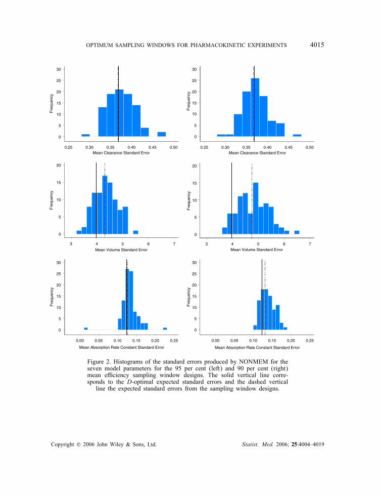
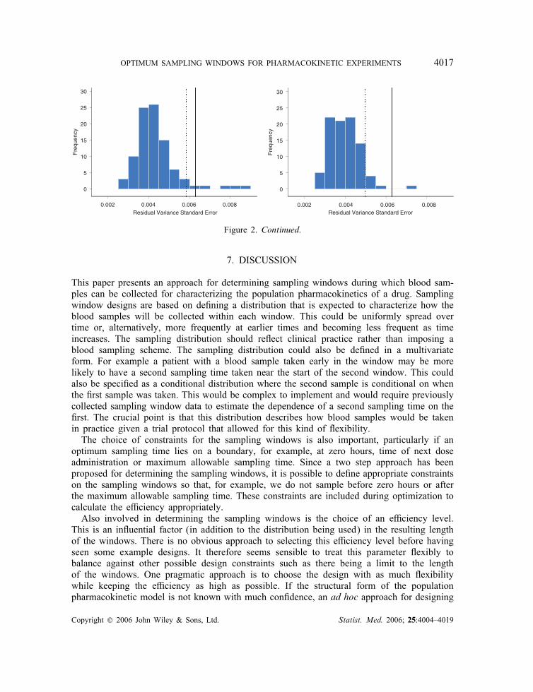
small upward bias and a small downward bias, respectively. The residual variance also showeda downward bias for both sampling window designs. The relative error on !2ka showed thelargest uncertainty of all the parameters.Figure 2 shows histograms of the estimated standard errors for the model parameters

obtained from NONMEM for both the 95 and 90 per cent mean e�ciency sampling win-dow designs. The standard errors were calculated for each simulated design as the square rootof the diagonal elements of the variance matrices. The expectation was then taken over alldesigns to give a single standard error for each parameter. This is di�erent from the criterionused to optimize the sampling window design but gives a good indication of the uncertaintyin the parameter estimates for such a design. In all cases, the expected standard errors fromthe 95 per cent sampling window design are closer to the D-optimum standard errors than forthose from the 90 per cent sampling window design. The sampling window design reducesthe standard errors for the residual variance and !2ka . The expected D-optimal and expectedsampling window standard errors for the residual variance are higher than that obtained fromthe NONMEM simulations, and the expected standard errors for !2V are mostly larger than



0.25 0.30 0.35 0.40 0.45 0.50 0.25 0.30 0.35 0.40 0.45 0.50

0

5

10

15

20

25

30

Mean Clearance Standard Error Mean Clearance Standard Error

Fre

quen

cy

10

0

5

15

20

25

30

Fre

quen

cy

0.00 0.05 0.10 0.15 0.20 0.25

0

5

10

15

20

25

30

0

5

10

15

20

25

30

Mean Absorption Rate Constant Standard Error

Fre

quen

cy

Fre

quen

cy

0.00 0.05 0.10 0.15 0.20 0.25

Mean Absorption Rate Constant Standard Error

0

5

10

15

20

Mean Volume Standard Error Mean Volume Standard Error

Fre

quen

cy

0

5

10

15

20

Fre

quen

cy

3 4 5 6 7 3 4 5 6 7

Figure 2. Histograms of the standard errors produced by NONMEM for theseven model parameters for the 95 per cent (left) and 90 per cent (right)mean e�ciency sampling window designs. The solid vertical line corre-sponds to the D-optimal expected standard errors and the dashed verticalline the expected standard errors from the sampling window designs.



0.005 0.010 0.015 0.020 0.025

Clearance Variance Standard Error

0.005 0.010 0.015 0.020 0.025

Clearance Variance Standard Error

Fre

quen

cy

Fre

quen

cy

0.010 0.015 0.020 0.025 0.030 0.035 0.040

0

5

10

15

20

25

Volume Variance Standard Error

Fre

quen

cy

0

5

10

15

20

25

Fre

quen

cy

Volume Variance Standard Error

0.010 0.015 0.020 0.025 0.030 0.035 0.040

10

0

20

30

10

0

20

30

Fre

quen

cy

0.00 0.05 0.10 0.15 0.20Absorption Rate Constant Variance Standard Error

40

30

20

10

0

0.00 0.05 0.10 0.15 0.20

Absorption Rate Constant Variance Standard Error

Fre

quen

cy

40

30

20

10

0

Figure 2. Continued.

that estimated by NONMEM. The standard deviation of the model parameter estimates forthe successful runs were 0.35 (Cl), 4.82 (V ), 0.13 (ka), 0.016 (!2Cl), 0.023 (!

2V ), 0.055 (!

2ka)

and 0.0039 (�2) for the 95 per cent sampling window design and 0.33, 5.24, 0.13, 0.017,0.030, 0.062 and 0.0039 for the 90 per cent sampling window design. These values are inapproximate agreement with those shown in Figure 2.



0.002 0.004 0.006 0.008

0

5

10

15

20

25

30

Residual Variance Standard Error

Fre

quen

cy

Residual Variance Standard Error0.002 0.004 0.006 0.008

0

5

10

15

20

25

30

Fre

quen

cy

Figure 2. Continued.

7. DISCUSSION

This paper presents an approach for determining sampling windows during which blood sam-ples can be collected for characterizing the population pharmacokinetics of a drug. Samplingwindow designs are based on de�ning a distribution that is expected to characterize how theblood samples will be collected within each window. This could be uniformly spread overtime or, alternatively, more frequently at earlier times and becoming less frequent as timeincreases. The sampling distribution should re�ect clinical practice rather than imposing ablood sampling scheme. The sampling distribution could also be de�ned in a multivariateform. For example a patient with a blood sample taken early in the window may be morelikely to have a second sampling time taken near the start of the second window. This couldalso be speci�ed as a conditional distribution where the second sample is conditional on whenthe �rst sample was taken. This would be complex to implement and would require previouslycollected sampling window data to estimate the dependence of a second sampling time on the�rst. The crucial point is that this distribution describes how blood samples would be takenin practice given a trial protocol that allowed for this kind of �exibility.The choice of constraints for the sampling windows is also important, particularly if an

optimum sampling time lies on a boundary, for example, at zero hours, time of next doseadministration or maximum allowable sampling time. Since a two step approach has beenproposed for determining the sampling windows, it is possible to de�ne appropriate constraintson the sampling windows so that, for example, we do not sample before zero hours or afterthe maximum allowable sampling time. These constraints are included during optimization tocalculate the e�ciency appropriately.Also involved in determining the sampling windows is the choice of an e�ciency level.

This is an in�uential factor (in addition to the distribution being used) in the resulting lengthof the windows. There is no obvious approach to selecting this e�ciency level before havingseen some example designs. It therefore seems sensible to treat this parameter �exibly tobalance against other possible design constraints such as there being a limit to the lengthof the windows. One pragmatic approach is to choose the design with as much �exibilitywhile keeping the e�ciency as high as possible. If the structural form of the populationpharmacokinetic model is not known with much con�dence, an ad hoc approach for designing



a study that will allow some model exploration would be to set the required e�ciency level alittle lower than otherwise considered. This could then be, in some sense, a measure of howmuch con�dence one has in the proposed model and how much the design can be tuned tothat model. The result of this would be to make the sampling windows wider.The optimum sampling window design method also takes into account the sample size

(number of subjects and number of observations per subject). This is achieved by choosingthe window length such that no more than 100× per cent sampled designs fall belowthe target e�ciency level, e�0. This has the e�ect of reducing the length of the samplingwindows for a given sample size but it also results in a more assured design of achieving therequired e�ciency level (assuming the model is correct). In the examples considered here,the e�ciencies were insensitive to the sample sizes chosen. However it is expected that asthe number of subjects decreases or variability in the model increases, the sampling windowdesign will be sensitive to the sample size.D-optimality was used as the reference criterion in this paper but there is no reason why

other optimality criteria could not be used, for example c-optimality (with an appropriatee�ciency calculation). Even Bayesian optimality criteria could be used that account for theuncertainty in the parameters or even model uncertainty. There may even be approaches wherethe uncertainty in the parameters is used as a means of calculating the sampling windows.Pronzato [26] approached the problem of estimating the position of the sampling windowsgiven that there is some measure of spread around the unknown design points that act aslocation points. This is an approach that could be applied to population pharmacokineticmodels. An alternative approach to calculating sampling windows in a population setting isto consider each subject as a realization from the population. Each of these subjects wouldhave their own optimum design. Amalgamating these individual designs would result in adistribution around some mean time vector, which could then be formulated as a samplingwindow design. Alternatively a population design could be optimized so that it is optimum forempirical Bayes estimation of each individual’s parameter vector. These alternative strategiesto the approach suggested in this article merit investigation in the future.

ACKNOWLEDGEMENTS

The Centre for Applied Pharmacokinetic Research (CAPKR) is funded by a consortium of pharmaceu-tical companies including Glaxosmithkline, P�zer, Novartis, Lilly and Servier. The authors would alsolike to thank two reviewers for comments that led to a greatly improved manuscript.

REFERENCES

1. van Bree J, Nedelman J, Steiner JL, Tse F, Robinson W, Niederberger W. Application of sparse samplingapproaches to rodent toxicokinetics: a prospective view. Drug Information Journal 1994; 28:263–279.

2. Sheiner LB, Rosenberg B, Marathe VV. Estimation of population characteristics of pharmacokinetic parametersfrom routine clinical data. Journal of Pharmacokinetics and Biopharmaceutics 1977; 5:445–479.

3. Aarons L, Vozeh S, Wenk M, Weiss P, Follath F. Population pharmacokinetics of tobramycin. British Journalof Clinical Pharmacology 1989; 28:305–314.

4. Racine-Poon A, Wake�eld J. Statistical methods for population pharmacokinetic modelling. Statistical Methodsin Medical Research 1998; 7:63–84.

5. Mandema JP, Verotta D, Sheiner LB. Building population pharmacokinetic models. I. Models for covariatee�ects. Journal of Pharmacokinetics and Biopharmaceutics 1992; 20:511–528.

6. Wake�eld J, Bennett J. The Bayesian modelling of covariates for population pharmacokinetic models. Journalof the American Statistical Association 1996; 91:917–926.



7. Holford NHG, Kimko HC, Monteleone JPR, Peck CC. Simulation of clinical trials. Annual Review ofPharmacology and Toxicology 2000; 40:209–234.

8. Gieschke R, Steimer JL. Pharmacometrics: modelling and simulation tools to improve decision making in clinicaldrug development. European Journal of Drug Metabolism and Pharmacokinetics 2000; 25(1):49–58.

9. Gomeni R, Bani M, D’Angeli C, Corsi M, Bye A. Computer-assisted drug development (CADD): an emergingtechnology for designing �rst-time-in-man and proof-of-concept studies from preclinical experiments. EuropeanJournal of Pharmaceutical Sciences 2001; 13:261–270.

10. Nestorov I, Graham G, Du�ull S, Aarons L, Fuseau E, Coates P. Modelling and simulation for clinical trialdesign involving a categorical response: A phase II case study with naratriptan. Pharmaceutical Research 2001;18:1210–1219.

11. D’Argenio D. Optimal sampling times for pharmacokinetic experiments. Journal of Pharmacokinetics andBiopharmaceutics 1981; 9:739–756.

12. Cherno� H. Locally optimal designs for estimating parameters. Annals of Mathematical Statistics 1953; 24:586.13. Kiefer J. Optimum experimental designs (with discussion). Journal of the Royal Statistical Society Series B

1959; 21:272–319.14. Fedorov VV. Theory of Optimum Experiments. Academic Press: New York, 1972.15. Atkinson AC, Donev AN. Optimum Experimental Designs. Clarenden Press: Oxford, 1992.16. D’Argenio. Incorporating prior uncertainty in the design of sampling schedules for pharmacokinetic parameter

estimation experiments. Mathematical Biosciences 1990; 33:105–118.17. Mentr�e F, Burton P, Merl�e Y, van Bree J, Mallet A, Steimer JL. Sparse sampling optimal designs in

pharmacokinetics and toxicokinetics. Drug Information Journal 1995; 29:997–1019.18. Mentr�e F, Mallet A, Baccar D. Optimal design in random e�ects regression models. Biometrika 1997; 84:

429–442.19. Tod M, Rocchisani JM. Comparison of, ED, EID, and API criteria for the robust optimisation of sampling times

in pharmacokinetics. Journal of Pharmacokinetics and Biopharmaceutics 1997; 25:515–537.20. Du�ull SB, Mentr�e F, Aarons L. Optimal design of a population pharmacodynamic experiment for ivabradine.

Pharmaceutical Research 2000; 18:83–89.21. Retout S, Mentr�e F, Bruno R. Fisher information matrix for non-linear mixed-e�ects models: Evaluation and

application for optimal design of enoxaparin population pharmacokinetics. Statistics in Medicine 2002; 21:2623–2639.

22. Aarons L, Balant LP, Mentr�e F, Morselli PL, Rowland M, Steimer JL, Vozeh S. Practical experience andissues in designing and performing population pharmacokinetic=pharmacodynamic studies. European Journal ofClinical Pharmacology 1996; 49:2623–2639.

23. Jonsson EN, Wade JR, Karlsson MO. Comparison of some practical sampling strategies for populationpharmacokinetic studies. Journal of Pharmacokinetics and Biopharmaceutics 1996; 24:245–263.

24. Hashimoto Y, Sheiner LB. Designs for population pharmacodynamics: value of pharmacokinetic data andpopulation analysis. Journal of Pharmacokinetics and Biopharmaceutics 1991; 19:333–353.

25. Green B, Du�ull SB. Prospective evaluation of a D-optimal design population pharmacokinetic study. Journalof Pharmacokinetics and Pharmacodynamics 2003; 30:145–161.

26. Pronzato L. Information matrices with random regressors. Application to experimental design. Journal ofStatistical Planning and Inference 2002; 108:189–200.

27. Retout S, Du�ull S, Mentr�e F. Development and implementation of the population Fisher information matrixfor the evaluation of population pharmacokinetic designs. Computer Methods and Programs in Biomedicine2001; 65:141–151.

28. Matlab User’s Guide version 6.1. The MathWorks: Natick, MA, 2001.29. Boeckman AJ, Sheiner LB, Beal SL. NONMEM users guide. NONMEM Project Group, University of

California, San Francisco, 1994.


optimum blood sampling time windows for parameter estimation in population pharmacokinetic...

Documents