U.S.N.A --- Trident Scholar project report; no.xxx (2001)

OPTIMIZING THE STRENGTH AND SCC RESISTANCE OF ALUMINUM ALLOYS USED FOR REFURBISHING AGING AIRCRAFT

by

Midshipman Charles P. Ferrer, Class of 2001 United States Naval Academy

Annapolis, Maryland

_______________________________________ (signature)

Certification of Advisers Approval

Associate Professor Angela L. Moran Mechanical Engineering Department

_______________________________________

(signature) _____________________

(date)

Assistant Professor Michelle G. Koul Mechanical Engineering Department

_______________________________________

(signature) _____________________

(date)

Acceptance for the Trident Scholar Committee

Professor Joyce. E. Shade Chair, Trident Scholar Committee

________________________________________

(signature) _____________________

(date)

USNA - 1531 -2

Form SF298 Citation Data

Report Date("DD MON YYYY") 07052001

Report TypeN/A

Dates Covered (from... to)("DD MON YYYY")

Title and Subtitle Optimizing the strength and SCC resistance of aluminum alloysused for refurbishing aging aircraft

Contract or Grant Number

Program Element Number

Authors Ferrer, Charles P.

Project Number

Task Number

Work Unit Number

Performing Organization Name(s) and Address(es) US Naval Academy Annapolis, MD 21402

Performing Organization Number(s)

Sponsoring/Monitoring Agency Name(s) and Address(es) Monitoring Agency Acronym

Monitoring Agency Report Number(s)

Distribution/Availability Statement Approved for public release, distribution unlimited

Supplementary Notes

Abstract

Subject Terms

Document Classification unclassified

Classification of SF298 unclassified

Classification of Abstract unclassified

Limitation of Abstract unlimited

Number of Pages 113

REPORT DOCUMENTATION PAGE

Form ApprovedOMB No. 074-0188

Public reporting burden for this collection of information is estimated to average 1 hour per response, including g the time for reviewing instructions, searching existing datasources, gathering and maintaining the data needed, and completing and reviewing the collection of information. Send comments regarding this burden estimate or any otheraspect of the collection of information, including suggestions for reducing this burden to Washington Headquarters Services, Directorate for Information Operations and Reports,1215 Jefferson Davis Highway, Suite 1204, Arlington, VA 22202-4302, and to the Office of Management and Budget, Paperwork Reduction Project (0704-0188), Washington, DC20503.

1. AGENCY USE ONLY (Leave blank) 2. REPORT DATE

7 May 20013. REPORT TYPE AND DATE COVERED

4. TITLE AND SUBTITLE

Optimizing the strength and SCC resistance of aluminumalloys used for refurbishing aging aircraft6. AUTHOR(S)

Ferrer, Charles P.

5. FUNDING NUMBERS

7. PERFORMING ORGANIZATION NAME(S) AND ADDRESS(ES) 8. PERFORMING ORGANIZATION REPORT NUMBER

9. SPONSORING/MONITORING AGENCY NAME(S) AND ADDRESS(ES) 10. SPONSORING/MONITORING AGENCY REPORT NUMBER

US Naval AcademyAnnapolis, MD 21402

Trident Scholar project report no.281 (2001)

11. SUPPLEMENTARY NOTES

12a. DISTRIBUTION/AVAILABILITY STATEMENT

This document has been approved for public release; its distributionis UNLIMITED.

12b. DISTRIBUTION CODE

13. ABSTRACT:The focus of this report is on the mechanical and corrosion properties of high-strength aluminum alloys. Aluminum alloy 7075,a common material in the aerospace industry, is susceptible to stress-corrosion cracking (SCC) in the T6, or peak-agedtemper. The susceptibility of this temper to SCC is alleviated through the use of the T73, or overaged temper. This temperexhibits significantly better SCC resistance, but at a 10-15% strength loss compared to the T6 temper. Cina and Ranishpatented a new heat treatment known as retrogression and reaging (RRA) in 1974. Experimental test results indicate that theRRA heat treatment reduces the traditional trade-off between T6 strength and T73 SCC resistance. However, the short timeheat treatment limits the applicability of RRA to thin sections of material. The primary goal of this research was todetermine if lower retrogression temperatures could be used in the RRA process to extend the applicability of this heattreatment to thick sections. Tensile, fatigue, fracture toughness, and hardness tests were conducted to characterize themechanical properties of the T6, T73, and various RRA tempers. Alternate immersion and double-cantilever beam tests wereconducted to evaluate the corrosion properties of the different tempers.

15. NUMBER OF PAGES111

14. SUBJECT TERMSStress corrosion cracking, aluminum alloys, heat treatment

16. PRICE CODE

17. SECURITY CLASSIFICATION OF REPORT

18. SECURITY CLASSIFICATION OF THIS PAGE

19. SECURITY CLASSIFICATION OF ABSTRACT

20. LIMITATION OF ABSTRACT

NSN 7540-01-280-5500 Standard Form 298 (Rev.2-89) Prescribed by ANSI Std. Z39-18

1

ABSTRACT

The focus of this Trident Research project is on the mechanical and corrosion

properties of high-strength aluminum alloys. Aluminum alloy 7075, a common material

in the aerospace industry, is susceptible to stress-corrosion cracking (SCC) in the T6, or

peak-aged temper. The susceptibility of this temper to SCC is alleviated through the use

of the T73, or overaged temper. This temper exhibits significantly better SCC resistance,

but at a 10-15% strength loss compared to the T6 temper.

Cina and Ranish patented a new heat treatment known as retrogression and

reaging (RRA) in 1974. Experimental test results indicate that the RRA heat treatment

reduces the traditional trade-off between T6 strength and T73 SCC resistance. However,

the short time heat treatment limits the applicability of RRA to thin sections of material.

The primary goal of this research was to determine if lower retrogression

temperatures could be used in the RRA process to extend the applicability of this heat

treatment to thick sections. Tensile, fatigue, fracture toughness, and hardness tests were

conducted to characterize the mechanical properties of the T6, T73, and various RRA

tempers. Alternate immersion and double-cantilever beam tests were conducted to

evaluate the corrosion properties of the different tempers.

Keywords: stress corrosion cracking, aluminum alloys, heat treatment

2

ACKNOWLEDGMENTS

I would like to express my sincerest gratitude to several individuals who helped

me to overcome the challenges of a Trident Scholar project. First, I would like to thank

Mr. Steve Crutchley and Mr. Anthony Antenucci. These two gentlemen were always

willing to lend me a hand in the Materials lab and provide an enjoyable work atmosphere.

Dr. Eui Lee and Mr. Dale Moore at Naval Air Station, Patuxent River, were very

helpful during my internship at the Becker Lab. I thank them for them for their useful

insight and enthusiasm about my research.

I thank Dr. Omar Es-Said for his insight on the heat treatment process. He was

extremely timely and thorough in responding to my questions.

Mr. Thomas Price and the gentlemen in the Rickover Hall machine shop helped to

prepare all of the specimens utilized for my testing and analysis. I thank all of these

individuals for their patience and willingness to assist me.

I would like to thank Dr. James Moran at ALCOA Technical Center for helping

me initiate the corrosion testing for my project. He went out of his way to help me

understand and properly conduct the experimentation.

Associate Professor Richard Link was a tremendous factor in helping me

understand the concepts of fracture mechanics and crack propagation. I thank him for the

countless hours he spent with me to ensure I was well versed on the methods and

standards required for this field of study.

3

Mr. Brian Connolly was extremely accommodating in helping me understand the

kinetics of heat treatment and the importance of microstructure on material properties. I

appreciate his generosity and enthusiasm.

I thank my parents who, as always, were very supportive of my efforts. They

have been extremely encouraging throughout this past year.

Associate Professor Angela Moran and Assistant Professor Michelle Koul were

my two advisors for this research project. I thank Professor Koul for her advice, ideas

and creativeness to help me through this year. Professor Moran’s experience, knowledge

and understanding were a significant help. I would like to express my utmost

appreciation for the time they spent to make the project a valuable learning experience for

me.

4

TABLE OF CONTENTS ABSTRACT ACKNOWLEDGEMENTS TABLE OF CONTENTS LIST OF FIGURES LIST OF TABLES 1.0 BACKGROUND 1.1 Aluminum Properties and Uses 1.2 Alloy Designations 1.3 Corrosion Resistance 1.4 Effect of Thermal Heat Treatment on Corrosion 1.5 Current Problems with Aluminum Alloys 1.6 Retrogression and Reaging Heat Treatment 1.7 Previous Trends Produced with the RRA Heat Treatment 1.8 Microstructural Trends in the RRA Heat Treatment 1.9 Conductivity Trends in the RRA Heat Treatment 1.10 Overall Trend with the RRA Heat Treatment 2.0 RESEARCH GOALS AND OBJECTIVES 3.0 EXPERIMENTATION 3.1 Materials 3.2 Heat Treatments 3.3 Initial Survey to Determine Candidate RRA Treatments 3.4 Hardness Measurements 3.5 Tensile Test 3.6 Fatigue Test 3.7 Fracture Toughness Test 3.8 Alternate Immersion Test 3.9 Double-Cantilever Beam (DCB) Test 3.10 Conductivity Measurements 4.0 RESULTS 4.1 Hardness Profile Results 4.2 Tensile Test Results 4.3 Fatigue Test Results 4.4 Fracture Toughness Test Results 4.5 Alternate Immersion Results 4.6 Double-Cantilever Beam Results 5.0 FOLLOW-ON EXPERIMENTATION 5.1 Conductivity and Hardness Measurements

5 5.2 Alternate Immersion Results from follow-on experimentation

5.3 Double-Cantilever Beam Results from follow-on experimentation 6.0 DISCUSSION 6.1 Stress Corrosion Cracking Behavior 6.2 Heat Transfer Analysis 7.0 CONCLUSIONS 8.0 RECOMMENDATIONS 9.0 APPENDICES 9.1 Tuning Procedure for Muffle Furnace

9.2 Fatigue Apparatus Tuning Procedure 9.3 Pre-cracking Procedure for Fracture Toughness Testing 9.4 Pre-cracking Procedure for DCB Test 9.5 Data From Double-Cantilever Beam Experiment

10.0 REFERENCES

6 LIST OF FIGURES

Figure 1. Temperature versus time diagram Figure 2. Aloha Airlines accident in 1988 Figure 3. Relationship between strength and stress-corrosion resistance Figure 4. Yield strength versus retrogression time plot Figure 5. Schematic of double-cantilever beam specimen Figure 6. Crack length versus time plot indicating the crack growth rate Figure 7. Crack growth rate versus stress intensity factor plot Figure 8. Plot of 0.2% yield strength versus crack growth rates Figure 9. Plot of hardness versus crack growth rate Figure 10. Scanning electron microscope (SEM) Figure 11. Conductivity versus retrogression time indicating the conductivity

variation with increasing retrogression time Figure 12. Yield strength versus retrogression time plot indicating the proposed

retrogression time for optimal conditions Figure 13. Schematic depicting the three directions on a rolled plate and the

orientation the samples were taken out of the plate Figure 14. Muffle furnace with five high-temperature J-type thermocouples Figure 15. Slow cut saw used for developing cubic test blocks Figure 16. Hardness testing apparatus Figure 17. Tensile test specimen Figure 18. Tensile test apparatus Figure 19. One-inch extensometer mounted on a tensile specimen Figure 20. Stress versus strain diagram for a tensile test. The parallel line is used to

determine the 0.2% yield stress Figure 21. Fatigue testing apparatus Figure 22. Fatigue specimen Figure 23. Cycle counter on fatigue apparatus Figure 24. Notched compact-tensile specimen for fracture toughness testing Figure 25. MTS Apparatus Figure 26. Load versus displacement plot during a fracture toughness test. The

straight line is .95 times the slope of the linear portion of the test data Figure 27. Failure of an alternate immersion specimen due to stress corrosion cracking (SCC) Figure 28. One-half inch extensometer mounted on an alternate immersion specimen Figure 29. Alternate immersion apparatus. The apparatus cycles alternate immersion

specimens in 3.5% NaCl for ten minutes of every hour Figure 30. Double-cantilever beam specimen Figure 31. Current source and voltmeter for conductivity measurements Figure 32. Conductivity specimen in sample holder Figure 33. Results of a Rockwell B (HRB) hardness profile for retrogression at

200°C for various times and for retrogression and reaging (RRA) Figure 34. Results of a Rockwell B (HRB) hardness profile for retrogression at

180°C for various times and for retrogression and reaging (RRA)

7 Figure 35. Results of a Rockwell B (HRB) hardness profile for retrogression at

160°C for various times and for retrogression and reaging (RRA) Figure 36. Plot of stress versus cycles to failure for 7075 aluminum Figure 37. Plot of stress versus cycles to failure for 7075 aluminum Figure 38. Plot of stress versus cycles to failure for 7075 aluminum Figure 39. Plot of stress versus cycles to failure for 7075 aluminum Figure 40. Plot of stress versus cycles to failure for 7075 aluminum Figure 41. Plot of stress versus cycles to failure for 7075 aluminum Figure 42. Results of alternate immersion test for 7075 aluminum Figure 43. Results of alternate immersion test for 7075 aluminum Figure 44. Results of alternate immersion test for 7075 aluminum Figure 45. Results of alternate immersion test for 7075 aluminum Figure 46. Results of alternate immersion test for 7075 aluminum Figure 47. Results of alternate immersion test for 7075 aluminum Figure 48. Crack growth rate versus stress intensity plot for 7075 aluminum Figure 49. Crack growth rate versus stress intensity plot for 7075 aluminum Figure 50. Crack growth rate versus stress intensity plot for 7075 aluminum Figure 51. Plot of HRB versus conductivity for 7075 aluminum in T6, T73, and

various RRA tempers Figure 52. Plot of HRB versus conductivity for 7075 aluminum Figure 53. Results of alternate immersion test for 7075 aluminum Figure 54. Results of alternate immersion test for 7075 aluminum Figure 55. Crack growth rate versus stress intensity plot for 7075 aluminum in T6,

T73, and RRA tempers Figure 56. Plot of 0.2% yield stress versus crack growth rate for 7075aluminum in

T6, T73, and various RRA tempers Figure 57a. SEM micrograph of 7075 aluminum in the T6 temper broken in laboratory

air Figure 57b. SEM micrograph of 7075 aluminum in the T6 temper broken in laboratory

air Figure 58a. SEM micrograph of 7075 aluminum retrogressed at 160°C for 660

minutes and reaged at 120°C for 24 hours broken in laboratory air Figure 58b. SEM micrograph of 7075 aluminum retrogressed at 160°C for 660

minutes and reaged at 120°C for 24 hours broken in laboratory air Figure 59a. SEM micrograph of 7075 aluminum in the T73 temper broken in

laboratory air Figure 59b. SEM micrograph of 7075 in the T73 temper broken in laboratory air Figure 60a. SEM micrograph of 7075 aluminum in the T6 temper exposed to 3.5%

NaCl by alternate immersion Figure 60b. SEM micrograph of 7075 aluminum in the T6 temper exposed to 3.5%

NaCl by alternate immersion Figure 61. Plate of thickness 2L immersed in fluid with a different temperature

8

LIST OF TABLES Table 1. Common aluminum alloy designations and

corresponding chemical composition of alloying elements Table 2. Position of Aluminum Alloys in Galvanic Series

compared to other common materials Table 3. Increase in resistivity due to the addition of alloying elements Table 4. Chemical composition of primary alloying elements of 7075

aluminum in the T6 and T73 tempers Table 5. Retrogression and reaging (RRA) heat treatments chosen for continued

testing Table 6. Tensile strengths of 7075 aluminum in the T6, T73, and various RRA

tempers Table 7. Results of fracture toughness tests on 7075 aluminum alloy in the T6, T73,

and RRA tempers. Table 8. Results of fracture toughness tests on 7075 aluminum alloy in the

T6, T73, and RRA tempers. Table 9. Theoretical temperature at the center and surface of a three-inch

cubic block of 7075 aluminum following the respective retrogression heat treatment.

9

1.0 BACKGROUND

1.1 Aluminum Properties and Uses

Aluminum has a wide variety of uses due to the combination of its favorable

properties. The properties that make aluminum so appealing include its high strength to

weight ratio, ease of formability, and high electrical and thermal conductivity. This metal

has experienced increasing levels of use in recent years and has replaced materials such

as wood, copper, and steel in many engineering applications.

Modern commercial and military aircraft owe many of their advances in design

and performance to the development of aluminum based alloys. The principal alloy of

this study, AA7075, is a high strength alloy used extensively for structural aircraft

components. This heat treatable, precipitate age hardened Al-Zn-Mg-Cu alloy remains

attractive for such applications primarily because of its high strength to weight ratio [1].

1.2 Alloy Designations

Engineering materials are often alloyed with various elements in order to produce

certain desired properties. Aluminum alloys are classified by the various alloying

elements that they contain. Under the supervision of the Aluminum Association (AA),

major aluminum producers have developed a four-digit numerical designation to classify

each of the different alloys. The first digit indicates the alloy group that contains specific

main alloying elements. 1XXX series alloys are primarily aluminum with a minimum Al

content of 99.0%. The main alloying elements for 2XXX, 3XXX, 4XXX, 5XXX, 6XXX,

10

and 7XXX series alloys are, respectively, copper, manganese, silicon, magnesium, both

magnesium and silicon, and zinc. The second digit designates the modification that was

done to the original alloy. The last two digits designate the specific aluminum alloy or

the purity of the aluminum in the case of 1XXX series alloys [2]. Table 1 lists common

aluminum alloy designations and their corresponding chemical compositions.

In addition to the four-digit number designating the types of aluminum alloys,

there is also a temper designation that is given to indicate the type of mechanical and/or

heat treatment that was performed on the material. The temper designations are separated

from the four-digit designation by a hyphen and subdivisions of each basic temper

are indicated through the

use of one or more

numbers. The basic temper

designations include F-(as

fabricated), O-(annealed),

H-(strain hardened), W-

(solution heat treated) and T-(stable thermal heat treatment).

Additional subdivisions of the T-(stable thermal heat treatment) are defined by an

added suffix digit that indicates secondary treatment used to influence the alloy’s

properties. T1 indicates a partial solution heat treat followed by natural aging treatment.

T3 indicates a solution heat treat followed by cold-work treatment. T4 indicates a

solution heat treat followed by natural aging treatment. T5 indicates an artificially aged

treatment only. T6 indicates a solution heat treat followed by an artificial aging

Alloy number

Chemical Composition (wt %)

2024 4.4 Cu, 1.5 Mg, 0.6 Mn 3003 1.2 Mn 5052 2.5 Mg, 0.25 Cr 6061 1.0 Mg, 0.6 Si, 0.27 Cu, 0.2 Cr 7075 5.6 Zn, 2.5 Mg, 1.6 Cu, 0.23 Cr

Table 1. Common aluminum alloy designations and corresponding chemical composition of alloying elements.

11

treatment. T7 indicates a solution heat treatment followed by stabilization or over-aged

treatment. T8 indicates a solution heat treatment followed by cold-work treatment

followed by artificial aging treatment. A second suffix digit has been used in the T7

temper to indicate further treatment in order to address specific desired properties. The

T73 temper was developed to provide additional resistance to stress corrosion cracking

(SCC), while the T76 temper was developed to provide additional resistance to

exfoliation.

The purpose of solution heat treatment is to place the maximum practical amount

of hardening solutes such as copper, magnesium, and zinc into solid solution in the

aluminum matrix. The artificial aging to produce the T6 temper is conducted in order to

accelerate the effect of precipitation on the mechanical properties of a material. The

purpose of artificial aging, or precipitation strengthening, is to create a large number of

hard particles per unit volume. The particles are obstacles to dislocation movement.

Impeding dislocation movement helps to increase the strength and hardness of the

material. The precipitation of 7075 aluminum occurs in the following sequence [3].

Supersaturated solid solution -> Guiner-Preston (GP) Zones ->

ηη ` (MgZn2) -> ηη (Mg Zn2)

The strength of rapidly quenched Al-Zn-Mg-Cu alloys aged at room temperature

to relatively low aging temperatures is the result of the formation of coherent, spherical

Cu-rich regions known as Guinier Preston (GP) zones. The GP zones are extremely

small, reaching a diameter of 12 Å after 25 years at room temperature. This

12

microstructure is representative of the W-temper. Yield strength in this temper increases

from approximately 138 MPa (20 ksi) to greater than 413 MPa (60 ksi) after ten years.

Extended artificial aging above room temperature, or precipitation hardening,

transforms the GP zones into the semi-coherent, transition precipitate η’, the precursor to

the equilibrium MgZn2 (η) phase. Temperatures of 115 to 130°C are used because the

material attains high strength in reasonably short times (24 hours for 2.5 cm thick plate).

At aging times and temperatures which produce peak strength properties of the T6

temper, the matrix microstructure consists of GP zones 20 to 35 Å in diameter in addition

to a small amount of η’. Yield strength increases from approximately 138 MPa (20 ksi)

in the quenched condition to greater than 572 MPa (83 ksi) as a result of the aging

treatment.

Figure 1 shows a temperature versus time diagram and the heat treatment steps to

obtain precipitation hardening. The figure shows that that the solution heat treatment is

completed at a higher temperature relative to the artificial aging temperature.

The T7 treatment usually involves a 2-step artificial aging treatment. An initial

low temperature aging treatment (i.e., 100 to 200°C) generates a large number of GP

zones that are stable at high temperatures. The GP zones transform to the meta-stable η’

precipitate and finally to the equilibrium η phase during the higher temperature (i.e., 160

to 177°C) overaging or stabilizing treatment [4].

13

1.3 Corrosion Properties of Aluminum Alloys

Aluminum, like all other metals, attempts to return to the lower energy state form

in which it occurs in nature. Corrosion is a general term that describes the oxidation

process a metal undergoes when returning to this lower energy level. Corrosion causes

changes in a metal that often become visible and have potential to cause serious damage.

The most recognizable form of corrosion occurs in iron where the product is iron oxide,

or rust. In aluminum, the corrosion product is hydrated aluminum oxide. This hydrated

oxide, also known as bauxite, is the form in which aluminum is found in the earth.

Therefore, aluminum, in its metallic state, will tend to return to bauxite.

Aluminum, as compared to many other metals such as copper, lead, and silver, is

considered an active metal due to its position in the galvanic series. Table 2 displays the

position of aluminum alloys in the galvanic series as compared to other common

Time

Tem

pera

ture

Solution heat treatment

Quench

Precipitation heat treatment

Figure 1. Temperature versus time diagram showing the steps for precipitation hardening.

14

materials. The figure indicates that aluminum is anodic and therefore active. In other

words, aluminum is a metal that is easily oxidized. However, a highly protective natural

oxide film keeps aluminum from oxidizing when it is in its metallic state. If the film is

destabilized, exposed aluminum spontaneously forms another film with oxygen from the

air.

Although this favorable characteristic makes aluminum appear as though it will

prevent its own corrosion, this is not necessarily the case. The presence of corrosive

environments and various loading conditions cause a number of different types of

corrosion in aluminum alloys. These include, but are not limited to localized corrosion,

fretting corrosion, general corrosion, intergranular corrosion, and stress corrosion.

Localized corrosion occurs

in occluded areas between

surfaces where there is

moisture and appears as

crevice corrosion and pitting

corrosion. Fretting corrosion

occurs due to the wearing of

the protective film caused by

two surfaces chafing

together. Exfoliation corrosion, which is a form of intergranular corrosion, occurs when

corrosion follows elongated grain paths. Stress corrosion cracking (SCC) is the cracking

caused by the combined effects of tensile loading and the presence of a corrosive

Platinum Gold

Titanium Silver

Copper Tin

Lead Aluminum Alloys

Zinc Magnesium and

Magnesium Alloys

Increasingly Inert (cathodic)

Increasingly Active (anodic)

Table 2. Position of Aluminum Alloys in the Galvanic Series compared to other common materials.

15

environment. When stress corrosion cracking initiates in a material, small cracks will

propagate in a direction perpendicular to the applied stress. These cracks often form at

stress levels well below a material’s tensile strength. One of the major problems with

SCC is that there is a frequently a lack of warning or detection. Catastrophic failure is

often the first sign of material degradation due to the environment [5].

The state of mechanical stress is a major factor that dictates whether stress

corrosion cracking will occur in materials. In most engineering applications, applied

loads will increase the local state of stress at the tip of an advancing crack. The state of

stress is often complicated due to the complex shape and design of structural materials.

The loading conditions range from tensile, shear, plane stress, and biaxial modes. All of

these factors create varied local stress and strain conditions at the crack tip and beyond

the crack front.

The type and extent of corrosion that occurs in metals also depends on the

environment. Different environmental conditions include rural, marine, and industrial

atmospheres as well as fresh water and seawater. The pH level, temperature, fluid

movement, and other characteristics of the environment also factor into the corrosion

process. Aluminum alloys are commonly used in seawater environments in applications

such as lifeboats and barges. United States Navy aircraft, many of which are constructed

using aluminum alloys, operate in close proximity to seawater environments for extended

periods of time [6].

16

1.4 Effect of Thermal Heat Treatment and Processing Techniques on Corrosion

Properties of Materials

In addition to the environmental conditions, an alloy’s microstructure

significantly affects the corrosion resistance. Microstructure is altered and assumes

certain characteristics based on the composition of the alloy, mechanical processing and

thermal treatments. Overall, the alloy’s constituents, grain size and orientation, heat

treatments, cold work, and other processing techniques factor into determining the

material’s reaction to a corrosive environment. Different tempers have varying responses

to stress corrosion cracking and some are more susceptible than others

Grain size and orientation have a particularly important effect on the corrosion

behavior of thick sections of aluminum when it is subjected to stress corrosion cracking.

Elongated grains are often developed parallel to the rolling direction in machined plates.

Because stress corrosion cracking is intergranular in nature, the preferential crack path is

along these elongated grain boundaries. When a static stress is applied normal to these

elongated grains in the presence of a corrosive environment, there is a greater chance that

SCC will occur in the material [7].

1.5 Current Problems With Aluminum Alloys

High-strength aluminum alloys are commonly used in a variety of applications

including extensive use in the aerospace industry. In the 1920’s and 1930’s, the 2000

series of aluminum alloys was utilized in some of the early aircraft. In the 1940’s, the

idea of using aluminum alloys that were alloyed with zinc and magnesium for even

17

higher strengths led to the development of 7075-T6. This particular alloy was first used

in the World War II bomber aircraft. As new commercial aircraft were being developed,

engineers continued to incorporate aluminum 7075-T6 because of its proven reliability

[8].

Despite the effectiveness of aluminum alloys in a variety of applications in the

recent past, the material has drawbacks. In particular, the high-strength aluminum alloys

have been shown to be highly susceptible to intergranular and stress corrosion cracking.

High corrosion susceptibility is a dangerous feature for an aircraft material because it will

have a greater chance of developing microflaws. The microflaws then have the potential

to grow and cause catastrophic failure in the material. An example of the problem of

corrosion attack on aircraft materials was seen with the Aloha Airline’s flight 243

accident in 1988. When the aircraft was in flight to Honolulu, Hawaii, it underwent a

catastrophic structural failure and lost a large section of its forward fuselage. Figure 2

Figure 2. Aloha Airlines accident in 1988.

18

shows the damage that the commercial airplane sustained. The United States National

Transportation Safety Board’s investigation of this incident indicated that corrosion

damage led to the failure of the fuselage. Corrosion damage not visible during routine

inspection was deemed to be a major cause of this accident [9].

More recent indications of the need to investigate the corrosion susceptibility of

materials are seen in military aircraft. U.S. Navy aircraft operate in extreme temperature

and salt water environments. Furthermore, the aircraft are often subject to impacts and

vibration during operation. These factors combine to create a significant corrosion threat

to the aircraft materials.

An additional problem for the military aircraft is the fact that their expected age is

being extended. Due to funding issues and resources, the aircraft are expected to operate

beyond their normal lifetimes. Therefore, the cost of refurbishment and the maintenance

hours continue to increase. In fact, the U.S. Navy estimated that the corrosion

maintenance costs for Naval aviation in fiscal year 1999 was approximately $1.2 billion.

Furthermore, the potential for failure due to increased corrosion problems is a direct

safety threat to the pilot and crew of the aircraft [10].

1.6 Retogression and Reaging Heat Treatment

One of the major problems with the aluminum 7075-T6 and other Al-Mg-Zn-Cu

high-strength alloys is that they are highly susceptible to stress-corrosion cracking. The

heat treatment steps utilized to obtain the T6 temper include a solution heat treatment at

approximately 480°C for 30-120 minutes, quenching to room temperature, and aging at

19

120°C for 24 hours. Over-aging aluminum 7075 involves heat treating the material to the

T73 temper. The T73 temper, which involves a two-step aging process at 105°C and

175°C following quenching, increases the stress corrosion cracking resistance, but this is

at a cost of a 10-15% strength loss. Therefore, it is clear that there is a trade-off in

strength and corrosion resistance when choosing between the T6 peak-aged temper and

the T73 overaged temper [11].

The trade-off in the T6 and T73 properties is visually depicted using the

relationship between precipitation hardening and resistance to SCC for 7000-series alloys

shown in Figure 3. The T6 temper corresponds to the point of maximum strength and

lower resistance to SCC. The T73 temper, which involves aging at a higher temperature,

corresponds to a point beyond the maximum strength, but with higher resistance to SCC.

[12].

Figure 3. Relationship between strength and stress-corrosion

resistance during aging of high-strength, 7000-series alloys.

AGING TIME AGING TEMPERATURE

STRENGTH (YIELD STRENGTH) (HARDNESS) RESISTANCE TO SCC (TIME TO FAILURE)

STRENGTH

RESISTANCE TO SCC

20

Many research efforts have been made in an attempt to alleviate the tradeoff

between high-strength and stress corrosion cracking resistance in high strength aluminum

alloys. Of note, Cina reported a heat treatment known as retrogression and re-ageing

(RRA), which he claimed gave the corrosion resistance of 7075 in the T73 temper while

maintaining T6 level strengths. The RRA heat treatment is applied to material already in

the T6 condition and involves a short-time treatment from 200-280°C followed by re-

ageing with similar conditions used to obtain the T6 temper. During the retrogression

heat treatment, strength falls rapidly to a minimum, increases again, and then falls off

with increasing retrogression time. After re-ageing, the T6 level strength can be obtained

up to a limiting retrogression time [13].

Figure 4 shows a plot of yield strength versus the amount of retrogression time for

the 7000 series of aluminum alloys. The retrogression treatment causes the strength of

the material to decrease below that of the material in the initial T6 temper. Park and

Ardell attributed this drop in strength to the dissolution of the η` precipitates in the

material. The subsequent increase in strength after the initial minimum is attributed

partly to the precipitation of the η precipitate. The final decrease in strength is attributed

to the general coarsening of the particles and thus an overall decrease in particle

concentration. Coarsening of precipitate particles generally decreases the strength of a

material.

The reaging step in the RRA process, which is similar to the artificial aging step,

is the same as the final heat treatment step that is applied to a material to obtain the T6

temper. Artificial aging is commonly applied to aluminum alloys in order to obtain an

21

increase in strength of the material. The reaging heat treatment is applied to a material

for the same reason. The increase in strength following the reaging treatment has been

attributed to the nucleation and growth of η` particles [14].

Cina claimed that processing materials to the minimum of the retrogression curve,

followed by reaging led to the optimal combination of T6 strength and T73 stress

corrosion cracking (SCC) resistance (Figure 4).

Figure 4. Yield strength versus retrogression time plot indicating the yield strength variation of a material following retrogression and following RRA.

Typical RRA Behavior

Retrogression Time

Yie

ld S

tren

gth

Retrogressed and Reaged (RRA) Retrogressed

T6

Maximum retrogression time to maintain T6 level strength

Optimal retrogression time according to Cina

22

Previous work by Rajan et al [13] indicates that the optimal conditions for the

RRA heat treated 7075 do not correspond to the local minimum on the retrogression

curve. Park [15] and Ural [16] produced results that agree with Rajan. They found

optimal conditions occur at the maximum retrogression time that retains T6 strength

(Figure 4).

In either case, the time of the retrogression heat treatment in a temperature range

of 200-280°C is less than ten minutes. This effectively limits the process to thin sections

of material. Later work indicated that retrogressing at lower temperatures down to 180°C

produced similar strength trends [17].

1.7 Previous Trends Produced With the RRA Heat Treatment

In order to determine potential RRA heat treatments to perform on the aluminum

7075, a preliminary literature survey was conducted to determine the trends of previous

research. The RRA heat treatment of 7000 series aluminum alloys have produced a

series of trends with respect to microstructural characterization, stress-corrosion cracking

properties, conductivity, and

strength properties.

Stress-corrosion crack

velocity is typically measured

through the use of a bolt-

loaded double cantilever

beam (DCB) specimen

Figure 5. Schematic of double-cantilever beam specimen indicating the direction of loading and crack propagation.

23

shown in figure 5. Each specimen is loaded and subjected to 3.5 % NaCl in order to

simulate a corrosive environment. Experimental data for this test is typically shown as

the crack growth rate (da/dt) versus mode I stress intensity factor (K). The crack length

in the DCB specimen is measured over time. With the given crack length versus time

plot from experimental measurements, the crack rate (da/dt) is readily calculated. Figure

6 shows a crack length versus time diagram. The slope of the curve, or crack growth rate

is obtained at a given time from this data.

The stress intensity factor, K, is a value that quantifies the stress distribution

around a flaw. The stress intensity for the DCB specimen is a function of material

properties, specimen geometry, and the crack length. For aluminum alloys, a typical plot

Crack Length vs Time

Time

Cra

ck L

eng

th

da/dt

Figure 6. Crack length versus time plot indicating the crack growth rate (da/dt) at a certain time.

24

of the crack growth rate versus stress intensity curve is shown in Figure 7. The Stage II

crack growth is the portion of the curve where the crack growth rate is constant and

independent of stress intensity. As the crack continues to propagate, the stress intensity

will become lower. Because the stress distribution is lower on the crack tip, the crack

growth rate decreases. At a certain value of stress intensity, the crack growth will

approach zero. This is the vertical portion of the curve on the crack growth rate versus

stress intensity plot. The value of the stress intensity at this point is known as the KISCC

value, or the critical stress intensity value for stress corrosion cracking. Theoretically,

this is the stress intensity below which stress corrosion cracking in the material should

not occur [18].

Those alloys with better resistance to SCC have a lower Stage II crack velocity

Typical SCC Behavior in Aluminum Alloys

Stress Intensity Factor (K)

Cra

ck G

row

th R

ate

Stage II Crack

KISCC

Figure 7. Crack growth rate versus stress intensity factor plot.

25

and a higher stress-corrosion cracking stress intensity factor (KISCC). Aluminum alloys in

T6 temper will have higher Stage II crack velocity and lower KISCC values as compared to

those in the T73 temper. Depending on the combination used, the RRA heat treatment

produces SCC characteristics that vary from the T6 to the T73 temper.

Retrogression times and temperatures from previous research are shown in

Figures 8 and 9. Figure 9 shows a plot of Rockwell B Hardness versus crack growth rate.

Prior work indicates that Rockwell B Hardness (HRB) directly correlates with 0.2% yield

strength in investigations of the RRA heat treatment. Therefore, the use of hardness

0.2% Yield Strength vs Crack Growth Rate

0

100

200

300

400

500

600

0.0E+00 1.0E-02 2.0E-02 3.0E-02 4.0E-02 5.0E-02 6.0E-02 7.0E-02 8.0E-02 9.0E-02

Crack Growth Rate (mm/h)

0.2%

Yie

ld S

tren

gth

(MP

a)

Fleck et al Park

T651

T7351

5 min/ 200C

1 min/ 220CT73

T6

Figure 8. Plot of 0.2% yield strength versus crack growth rates for T6, T73, and various RRA tempers.

26

measurements gives a good characterization of the relative strength of the material for

different retrogression times. HRB measurements are described in section 3.4.

The optimal conditions are those that correspond to a low crack velocity

(comparable to T73 SCC resistance) and high strength (comparable to T6). The trends

indicate that at a specified temperature, stress corrosion crack velocity decreases with

increasing retrogression times. That is to say, increasing the retrogression time

corresponds to increased stress corrosion cracking resistance. This is in agreement with

Park et al [14] and Ural [16].

HRB vs Crack Growth Rate

86

87

88

89

90

91

92

93

94

0.0E+00 5.0E-03 1.0E-02 1.5E-02 2.0E-02 2.5E-02

Crack Growth Rate (mm/h)

Har

dnes

s (H

RB

)

Ural Park

25 min/ 200 C35 min/ 200 C

60 min/ 200 C80 min/ 200 C

T6

1 min/ 220 C

25 sec/ 240 C1 min/ 240 C

Figure 9. Plot of hardness versus crack growth rates for T6, T73, and various RRA tempers.

27

1.8 Microstructural Trends in the RRA Heat Treatment

Researchers have established mictrostructural characterizations of the RRA

treatment through the use of scanning electron microscopy (SEM) and transmission

electron microscopy (TEM). Figure 10 shows a scanning electron microscope. SEM

micrographs of surfaces are conducted through the use of two different types of electrons.

The secondary electrons increase the visibility of topographical features while the higher-

energy backscattered electrons show compositional variations across the surface. SEM is

advantageous due to easy specimen preparation and the ability to view a wide range of

magnifications. However, resolution and magnification are limited as compared to the

TEM. TEM is utilized when ultra fine detail is required. TEM analysis assumes a

homogenous microstructure as a function of macroscale; the limited examination area

should be representative of the microstructure throughout the material. The major

disadvantages of TEM are long specimen preparation time and limited examination area

per specimen [4].

Rajan et al [13], Park [15], Kanno et al [11], Wallace et al [19], Uguz et al [20]

and Thompson et al [21] have shown that the more corrosion resistant T73 temper has a

microstructure that is significantly different from that of the T6 temper. In general, the

microstructure of aluminum in the T73 temper has grain boundary precipitates that are

much coarser and larger than those of the T6 temper. Park et al [14] utilized measuring

parameters as a means of comparing different microstructures. He measured (1) the areal

fraction covered by particles on grain boundaries (AA) , (2) the number of particles per

unit area (NA), and (3) the mean particle size (dg). Particle volume fraction (VA), is a

28

function of the areal fraction (AA) and the number of particles per unit area (NA). Park

has shown that the steady-state crack growth velocity tends to decrease with increasing

AA and VA, and decreasing NA.

Increasing AA and VA means that the precipitate particles, η and η`, are covering

a larger area and have a larger volume. Decreasing NA means there are less precipitates

per unit area. Therefore, an increase in precipitate size directly correlates with increased

stress corrosion cracking resistance.

Thompson et al [21] hypothesized that the increased size of the grain boundary

precipitates creates a smaller cathode to anode ratio. In this sense, the stress corrosion

cracking behavior along the grain boundaries is analogous to the galvanic corrosion

Figure 10. Scanning electron microscope (SEM).

29

between dissimilar metals. A smaller cathode to anode ratio in galvanic corrosion creates

a lower current density. In general, a lower current density correlates with a lower rate of

corrosion. Therefore, the smaller precipitates in the T6 temper create a large cathode to

anode ratio and thus an increased susceptibility to corrosion.

Although the previous research has indicated these trends, the grain boundary

precipitate size in the mictrostructure may not be the only parameter that controls stress-

corrosion cracking in aluminum alloys. A complete characterization of all of the

microstructural parameters that affect stress corrosion cracking has yet to be determined.

1.9 Conductivity Trends in the RRA Heat Treatment

Additional investigations of the RRA heat treatment indicate that particles in the

7000 series aluminum alloys grow and coarsen during the retrogression. Furthermore,

Wallace et al [19] and Robinson et al [22] have shown that electrical conductivity

increases with increasing retrogression time. Electrical conductivity measurements are

commonly expressed as a percentage of the International Annealed Copper Standard

(%IACS). In general, an increase in electrical conductivity of aluminum alloys

corresponds to overaging of the material. In terms of conductivity, aluminum in the T73

temper typically has a significantly higher conductivity than aluminum in the T6 temper.

The T73 temper is around 40% IACS, while the T6 temper is around 30% IACS. This is

expected due to the overaged nature of the T73 temper as compared to the peak-aged

nature of the T6 temper.

30

Alloying elements have a strong effect on the conductivity (inverse of resistivity)

of a metal. For small concentrations of elements in solid solution in aluminum, it has

been found that the resistivity changes according to [23]

[ ]∑+=j

j jK %0ρρ

where

ρ0= the resistivity of the pure metal Kj = the change of electrical resistivity in the presence of 1% of element j %j= the concentration of element j in the alloy

It has been observed that the effect of an element on the resistivity of the alloy is

an order of magnitude smaller when the element is incorporated within a secondary phase

particle compared to the solid solution [24]. Table 3 displays the effect of alloying

elements on the resistivity in both solid solution and in the secondary phase [25].

As an alloy undergoes an aging treatment, second phase precipitates readily nucleate and

coarsen with time. With increasing aging time the volume fraction of the precipitate

phase grows due to enhanced nucleation and coarsening. This results in

the depletion of the supersaturated alloying elements in solid solution. Secondary phase

nucleation and subsequent coarsening can, therefore, be correlated with a decrease in

resistivity (increase in conductivity) as a function of aging time.

31

Figure 11 shows the relative conductivity differences between aluminum 7075 in

the T73 temper compared to the T6 temper. The figure indicates that increasing the

retrogression time during the RRA heat treatment corresponds to an increase in electrical

conductivity. Thus, it appears that there is a direct relationship between electrical

conductivity and stress-corrosion cracking resistance. That is, an increase in electrical

conductivity corresponds with an increase in corrosion resistance of the material.

Furthermore, previous research indicates that the reaging step in the RRA process

increases the conductivity about 1 to 2% IACS.

Resistivity Increase (ΩΩ m * 10-8) by adding 0.1% of an Impurity Element

Element

In Solid Solution Incorporated into Secondary Phase

B 0.08 -- Cr 0.40 0.02 Cu 0.032 0.003 Fe 0.26 0.006 Mg 0.05 0.02 Mn 0.29 0.03 Ni 0.08 0.006 Si 0.10 0.009 Ti 0.29 0.01 V 0.40 0.03 Zn 0.01 0.002 Zr 0.17 0.004

Table 3. Increase in resistivity due to the addition of alloying elements.

32

1.10 Overall Trend with the RRA Heat Treatment

Figure 12 shows the typical strength variation of aluminum alloys subjected to the

retrogression and reaging heat treatment. The figure indicates that there is a limiting

retrogression time where T6 level strength can still be obtained during the heat treatment

process. This time is dependent on the retrogression temperature utilized. Although Cina

and Ranish utilized temperatures greater than 200°C for the retrogression process, it has

been shown that the similar strength variations occur with the use of lower temperatures.

The kinetics of the reaction are retarded with lower retrogression temperatures [19]. In

other words, the lower the retrogression temperature, the longer time it takes for a

material to reach the limiting time to maintain T6 level strength. Longer retrogression

Typical conductivity behavior

Retrogression Time

Co

nd

uct

ivit

yT73 conductivity

T6 conductivity

Figure 11. Conductivity versus retrogression time indicating the increase in conductivity with increasing retrogression time.

33

times would be an advantage in that it would allow the RRA heat treatment to be

performed on thick sections.

Due to the nature of the trends of increasing conductivity, precipitate changes, and

strength variations that occur during the retrogression and reaging process, it is

hypothesized that the optimal retrogression time at a given temperature is the maximum

amount of time that still retains T6 level strength. This is because the T6 level strength is

still maintained while increasing the aging and thus the stress corrosion cracking

resistance of the material.

Typical RRA Behavior

Retrogression Time

Yie

ld S

tren

gth

Retrogressed and Reaged (RRA) Retrogressed

T6

Proposed retrogression time for optimal conditions

Optimal retrogression time according to Cina

toptimal, Cina toptimal, Ferrer

Figure 12. Yield strength versus retrogression time plot indicating the proposed retrogression time for optimal conditions.

34

2.0 RESEARCH GOALS AND OBJECTIVES

There is general disagreement in the literature as to what the optimal RRA heat

treatment conditions are for 7075 aluminum. Also, the mechanisms that are responsible

for the properties of an RRA heat-treated material are disputable. Furthermore, the RRA

heat treatment originally proposed by Cina is applicable only to thin sections. If an RRA

heat treatment can be applied to in-service parts, this will be an inexpensive way to

improve the safety and lifetimes of aircraft parts made of 7075 aluminum.

This research focused on the use of lower temperatures during the retrogression

step so that the heat treatment is applicable to thick sections. Various mechanical tests

and stress corrosion tests were performed on the retrogressed and reaged 7075 aluminum.

The properties of the RRA treatment are compared to the T6 and T73 tempers to

determine whether the lower retrogression temperatures in the RRA heat treatment help

to alleviate the traditional trade-off between the T6 and T73 tempers.

There are many alterations that can be made to the RRA heat treatment and it can be

applied to a variety of different aluminum alloys. Therefore, the focus of this research is

to continue the RRA testing based on the trends produced through previous research.

The project contributes to the literature database for RRA treated materials and attempts

to further explain the mechanisms that are responsible for the measured material

properties.

The goals of the research and experimentation were as follows.

35

• Perform various RRA heat treatments on 7075 aluminum using lower

retrogression temperatures and longer retrogression times than observed in the

literature.

• Conduct hardness, tensile, fatigue, conductivity, fracture toughness,

double-cantilever beam, and alternate immersion tests to compare the

mechanical and corrosion properties of 7075 aluminum in the various

tempers.

• Evaluate the feasibility of performing the RRA heat treatment on thick

section, commercially produced product forms.

36

3.0 EXPERIMENTATION

3.1 Materials

Aluminum 7075 was received in three-inch thick plates in both the T6 and T73

tempers. All of the specimens for testing were machined from the “as received”

condition prior to further heat treatment. Table 4 indicates the composition of the 7075

aluminum in the T6 and T73 tempers, both of which are within the chemical

specifications established for this particular alloy.

% Zn % Mg % Cu % Cr T6 Plate 5.93 2.28 1.57 0.21 T73 Plate 5.72 2.48 1.70 0.20

The plates received from the manufacturer were worked such that the material

developed characteristic grain orientations. Figure 13 shows the grain characterization of

the material and orientations for the specimens taken out of the plate. The longitudinal

(L), transverse (T), and short transverse (S) directions are shown on a rectangular section

of material. The longitudinal direction is the direction the plate as rolled during

production. The weakest or most susceptible direction of the material occurs when a

load is applied in the short transverse direction, and the crack growth is in the

longitudinal direction. All the specimens were machined such that the most susceptible

orientation was evaluated.

Table 4. Chemical composition of primary alloying elements of 7075 aluminum in the T6 and T73 tempers.

37

3.2 Heat Treatments

RRA heat treatments were conducted on the material in the T6 temper. This is

consistent with previous research where the RRA heat treatment was applied to material

received in the T6 condition. The RRA heat treatments were conducted using a

THERMOLYNE muffle furnace. Five J-type high temperature thermocouples were

spaced evenly around the furnace to monitor the temperature of the furnace and the test

samples. Figure 14 shows the placement of the thermocouples in the muffle furnace.

In order to increase the consistency and accuracy of the THERMOLYNE furnace, it was

tuned at each of the different temperatures that were utilized for heat treating the

aluminum. This tuning procedure is described in section 9.1.

Figure 13. Schematic depicting the three directions on a rolled plate and the orientation the samples were taken out of the plate.

Transverse

Longitudinal (Rolling direction)

Short Transverse

38

3.3 Initial Survey to Determine Candidate RRA Treatments

The initial survey of the retrogression and reageing heat treatment was done on

one-inch cubic test blocks. These cubic test blocks were taken from the T6 plate through

the use of an ISOMET 4000 slow cut saw. The slow cut saw is shown in Figure 15. The

test blocks, which were initially in the T6 condition, were retrogressed (heat treated) at

200, 180, and 160°C for various times. These retrogression temperatures were chosen

based on the trends determined from the literature, since a goal of this research was to

extend the evaluations at lower retrogression temperatures.

Figure 14. Muffle furnace with five high-temperature J-type thermocouples.

39

Following the

retrogression heat treatments,

all of the blocks were reaged

for 24 hours at 120°C. This

reaging treatment is the same

artificial aging treatment that

is applied to materials to give

the high-strength T6

condition. Based on

previous research, altering

the time of the reaging heat

treatment had a relatively minor effect on the strength and corrosion properties of

aluminum. Therefore, this variable was not investigated in this research and was kept

constant for all of the RRA heat treatments.

3.4 Hardness Measurements

Hardness is the measure of a material’s resistance to localized plastic

deformation. Hardness tests are very convenient and are often performed on materials in

lieu of more complex and time consuming testing. The reason is because the test is

simple, inexpensive, and non-destructive. Furthermore, other mechanical properties such

as tensile strengths correlate to hardness values.

Figure 15. Slow cut saw used for developing cubic test blocks.

40

Prior to the hardness

measurements, test blocks

were polished to ensure

smooth and flat surfaces.

Figure 16 shows the

INSTRON apparatus that was

utilized to test the hardness of

materials. The apparatus has a

small indenter that is forced

into the surface of the material.

The depth or size of the

resulting indentation is

measured, which yields a

hardness number. A larger and deeper indentation corresponds to a softer material, and

therefore a lower hardness value for the material.

There are various scales that are used when determining numerical values for

the hardness of a material. The Rockwell B Hardness (HRB) scale was utilized to

determine the hardness of the Aluminum 7075 since previous researchers utilized this

scale when determining the hardness variation with respect to varying retrogression

times. The HRB test involves the use of a 1/16-inch ball and a 100 kilogram load. The

HRB value is determined from the difference in depth of penetration in the material from

the application of a initial minor load followed by the a subsequent major load [26].

Figure 16. Hardness testing apparatus.

41

3.5 Tensile Tests

Tensile tests of the 7075 aluminum were conducted in the T6, T73, and the

various RRA treated samples. The test is in accordance with ASTM standard B 557M-94

[27]. This test was conducted in order to compare the strengths of the aluminum in the

various heat treatments. Tensile tests reveal the important parameters of yield strength,

ultimate tensile strength, and stiffness. The main purpose of the RRA treatment is to

maintain T6 level strengths while improving corrosion resistance. This particular test

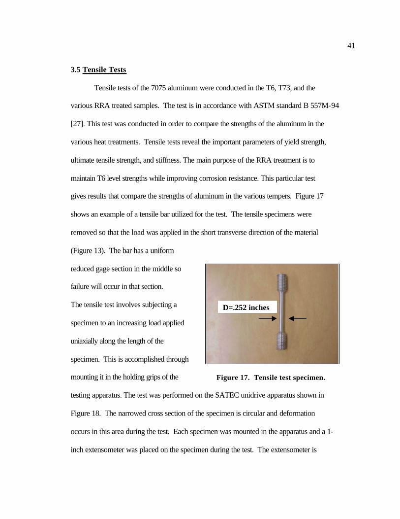
gives results that compare the strengths of aluminum in the various tempers. Figure 17

shows an example of a tensile bar utilized for the test. The tensile specimens were

removed so that the load was applied in the short transverse direction of the material

(Figure 13). The bar has a uniform

reduced gage section in the middle so

failure will occur in that section.

The tensile test involves subjecting a

specimen to an increasing load applied

uniaxially along the length of the

specimen. This is accomplished through

mounting it in the holding grips of the

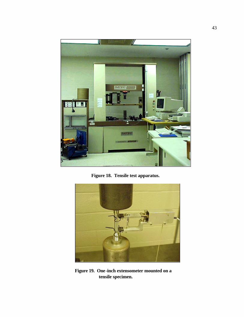
testing apparatus. The test was performed on the SATEC unidrive apparatus shown in

Figure 18. The narrowed cross section of the specimen is circular and deformation

occurs in this area during the test. Each specimen was mounted in the apparatus and a 1-

inch extensometer was placed on the specimen during the test. The extensometer is

Figure 17. Tensile test specimen.

D=.252 inches

42

utilized to measure the elongation, or strain, of the tensile bar. Figure 19 shows the

extensometer mounted on the tensile specimen. The apparatus elongated the specimen at

a constant rate and continuously measured the load and the elongation. The output of the

apparatus is an engineering stress versus engineering strain diagram.

Engineering stress, σ, is defined as

σ =FAO

Where F is the load applied perpendicular to the cross-sectional area and A0 is the initial

cross-sectional area of the specimen before any load was applied.

Engineering strain, ε, is defined as

ε =−l ll

i o

o

where li is the instantaneous gage length of the specimen and lo is the original gage length

of the specimen before the load was applied. The tensile test was performed until failure

for two specimens per heat treatment condition. The results of the tensile test allow for

the determination of the yield strength. The yield strength for each specimen was

determined through the 0.2% offset method.

43

Figure 19. One-inch extensometer mounted on a

tensile specimen.

Figure 18. Tensile test apparatus.

44

From the stress-strain diagram, an offset of 0.002 is measured from the start of the

test (zero stress and strain). A line parallel to the elastic portion of the test (linear portion

on the stress-strain diagram) was placed on the curve. The exact slope of this line was

determined through a regression analysis on the data. The point where the offset line

intersects the curve on the stress-strain diagram indicated the 0.2% yield stress of the

material. Figure 20 shows a stress versus strain diagram for a tensile test. The offset line

is shown parallel to the linear portion of the data.

Stress vs Strain

0.00E+00

1.00E+04

2.00E+04

3.00E+04

4.00E+04

5.00E+04

6.00E+04

7.00E+04

8.00E+04

9.00E+04

1.00E+05

0.0000 0.0010 0.0020 0.0030 0.0040 0.0050 0.0060 0.0070 0.0080 0.0090 0.0100

Strain (in/in)

Str

ess

(psi

)

.2 % Yield Strength

Figure 20. Stress versus strain diagram for a tensile test. The parallel line is used to determine the 0.2% yield stress.

45

3.6 Fatigue Test

Fatigue is a type of failure that occurs in materials when they are subjected to

fluctuating loads. Due to the fluctuating loads, structures are susceptible to failure at

much lower than expected load levels compared to static load conditions. The term

fatigue is utilized because failure of the material will occur after a long period of repeated

load cycling. Common examples of structures that undergo fatigue loading are bridges,

machine parts, and aircraft. Fatigue properties of materials are very relevant and

important to study because the majority of failures that occur in structures are due to

fatigue. In fact, it is this mode of failure that comprises almost 90% of failures in metals.

There are laboratory simulation tests to characterize the fatigue properties of

materials. The data is typically shown as stress amplitude (S) versus the number of

cycles to failure (N). This plot is known as an S-N curve. A higher magnitude of stress

on the specimen translates to a smaller number of cycles to failure. The S-N curves for

many ferrous materials become horizontal at lower stress levels. The value of stress at

this point is known as the endurance limit, or the stress below which fatigue failure will

not occur. Aluminum alloys typically do not exhibit an endurance limit and therefore are

often subject to fatigue failure [2].

The SATEC fatigue testing apparatus produces a sinusoidal vibratory force on a

fatigue specimen. Figure 21 shows the apparatus utilized for fatigue testing. In order to

produce the force, a rotating mass (eccentric), which is driven by synchronus motor,

rotates around a fixed axis. The centrifugal forces applied to the specimen are adjusted

through changing the distance the rotating mass (eccentric) spins from its axis of rotation.

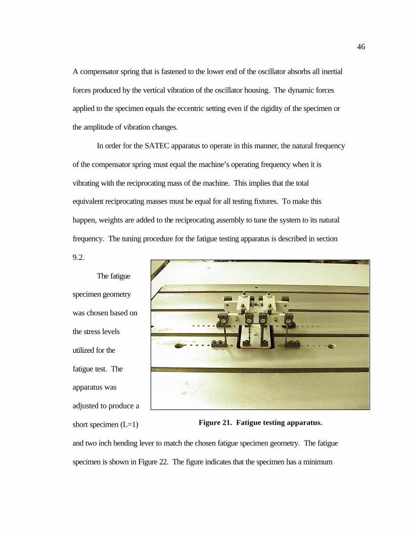
46

A compensator spring that is fastened to the lower end of the oscillator absorbs all inertial

forces produced by the vertical vibration of the oscillator housing. The dynamic forces

applied to the specimen equals the eccentric setting even if the rigidity of the specimen or

the amplitude of vibration changes.

In order for the SATEC apparatus to operate in this manner, the natural frequency

of the compensator spring must equal the machine’s operating frequency when it is

vibrating with the reciprocating mass of the machine. This implies that the total

equivalent reciprocating masses must be equal for all testing fixtures. To make this

happen, weights are added to the reciprocating assembly to tune the system to its natural

frequency. The tuning procedure for the fatigue testing apparatus is described in section

9.2.

The fatigue

specimen geometry

was chosen based on

the stress levels

utilized for the

fatigue test. The

apparatus was

adjusted to produce a

short specimen (L=1)

and two inch bending lever to match the chosen fatigue specimen geometry. The fatigue

specimen is shown in Figure 22. The figure indicates that the specimen has a minimum

Figure 21. Fatigue testing apparatus.

47

test area where failure will to occur during the fatigue test. This is analogous to the

minimum test area on the tensile specimens. Each fatigue specimen was machined from

the plate so that the reduced gage was loaded in the S direction and the fatigue cracks

grew in the L direction (Figure 13).

The eccentric was set to produce a pre-determined alternating stress on the

specimen based on the following equation.

PbSh

R=

2

3

where P=required force setting on eccentric b=specimen width at minimum test section R=bending leverage h=specimen thickness S=maximum bending stress

Fatigue tests were conducted for the

T6, T73, and the various RRA

tempers. Maximum stress values of

20, 25 and 30 ksi were utilized for

testing. Six fatigue tests per stress

were conducted for each temper.

The stress amplitude is calculated based on the specimen geometry and the properties of

the fatigue testing apparatus. Fatigue specimens were loaded and tested until failure at

Figure 22. Fatigue specimen.

3 in.

48

various stress levels. The fatigue apparatus automatically recorded the number of cycles

to failure for each specimen. The counting device on the SATEC fatigue testing

apparatus is shown in Figure 23.

The average value and sample

standard deviation of cycles to

failure for each temper at each

load was determined.

The data was plotted as the

mean value of cycles to failure

(N) with error bars that

correspond to standard

deviation of N.

The mean value of cycles to failure (Nm) was determined in the following manner.

Nn

Nm ii

n

==

∑1

1

Where Ni=value of sample i n=number of samples

The sample standard deviation, ∆N, of cycles to failure was determined as follows.

Figure 23. Cycle counter on fatigue apparatus.

49

∆ NN N

n

i mi

n

=−

−

=∑ ( )

/

2

1

1 2

1

Where Nm=mean value of N Ni=value of sample i n=number of samples

This standard deviation is also known as the unbiased or sample standard deviation. The

expression has n-1 instead of n in the denominator because only six specimens were

tested at each load. Standard deviation (where the expression has n in the denominator)

is used when at least twenty measurements are made [28].

3.7 Fracture Toughness Testing

The brittle failure of materials that are typically ductile in nature is studied in the

field of fracture mechanics to assess the relationship of the influence of flaws on crack

initiation and propagation. Aluminum, like many other materials, will contain both

macroscopic and microscopic flaws that have the potential to cause catastrophic failure.

Therefore, a detailed characterization of the fracture properties of aluminum is important

[2].

There are three basic modes in which a load can operate on a crack. Mode I is an

opening or tensile mode, mode II is a sliding, and mode III is a tearing mode. Mode I is

the loading method that is encountered the most and will be addressed here. The stresses

near a crack tip can be defined in terms of a stress intensity factor, K. The stress intensity

factor provides a specification of the stress distribution around a flaw. Since the stresses

50

near the crack tip can be defined in terms of the stress intensity factor, a critical value of

K exists. This critical value is used to specify the loading conditions and flaw size for

brittle fracture and is known as the fracture toughness, KC. The geometry-independent

value of KC for thick specimens is known as the plain strain fracture toughness, KIC. The

I in the subscript indicates that the critical value for the stress intensity is for mode I

loading conditions. Brittle materials tend to have low KIC values because plastic

deformation is not possible in front of an advancing crack tip. On the other hand, ductile

materials have relatively large KIC values. The critical stress intensity factor is related to

a stress intensity in the same manner that a stress is related a material’s yield strength. A

material may sustain a certain level of stress, but at a specific stress level it will

plastically deform. Similarly, a material will sustain variety of stress intensities, but at

the critical stress intensity factor, brittle fracture will occur.

Notched compact-tension (C-T) specimens were used to determine the fracture

toughness in air of the

aluminum 7075 in various heat

treated conditions. The

compact-tensile specimen is

shown in Figure 24.

Experience has indicated that a

machined notch does not

necessarily produce a natural

crack that is acceptable for a Figure 24. Notched compact-tensile specimen

used for fracture toughness testing.

2.4 in

51

reproducible result. In order to assist in alleviating this problem, a starter crack notch is

extended beyond the notch. This starter notch is called a pre-crack. The specimens were

pre-cracked using fatigue loading according to the ASTM standard E399 [29]. The

technique utilized for the pre-cracking is described in section 9.3.

Following pre-cracking, the specimens were loaded in the MTS apparatus shown

in Figure 25. The specimens were subjected to a continually increasing load until

fracture. During the test, load (P) and crack opening displacement (v) were recorded.

Crack opening displacement is the deflection of the notched end of the specimen during

loading and is measured by a clip gage.

Figure 25. MTS Apparatus

52

Once the data was collected for each test, it was analyzed to determine the KIC

value. A secant line is drawn through the origin of the test record with a slope equal to

0.95 (P/v)o, where (P/v)o, is the slope of the tangent OA to the linear portion of the data.

Figure 26 shows a load versus crack opening displacement plot for a fracture toughness

test. The intersection of the two curves corresponds to the load, PQ.

Once PQ is determined for the specimen, KQ is calculated in the following manner:

KP

BWf a WQ

Q= 1 2/ ( / )

Fracture Toughness Data

0

2000

4000

6000

8000

10000

12000

0.00 0.01 0.01 0.02 0.02 0.03 0.03 0.04 0.04 0.05 0.05

Displacement (inches)

Load

(lbs

)

PQ

Figure 26. Load versus crack opening displacement plot during a fracture toughness test. The straight line is .95 times the slope of the linear portion of the test data.

53

f a Wa W a W a W a W a W

a W( / )

( / )(. . / . / . / . / )( / ) /=

+ + − + −−

2 886 464 13 32 14 72 5 61

2 2 3 3 4 4

3 2

where

PQ=load as determined from the load versus crack opening displacement plot B= specimen thickness (approximately 1 inch) W=specimen width (load line to the back of the sample)

a=initial crack length (load line to the end of the fatigue pre-crack)

Once a value for KQ has been determined, the following must be calculated for further

determination of test validity.

252

.KQ

YSσ

where

σYS=material 0.2% yield strength

This value must be less than the specimen thickness, B, and the crack length in order for

KQ to equal KIC, and for the measured fracture toughness value to be independent of

specimen thickness.

3.8 Alternate Immersion Test

A number of service failures began to increase in the 1960’s when higher strength

alloys were utilized for service performance. The corrosion tests use accelerated methods

as ranking criteria for different alloys and various heat treatments. Various methods

currently used are all aimed at producing results that better correlate with service

54

performance. Stress corrosion cracking data must always be related to the type of alloy,

heat treatment, and the environment that was utilized to accelerate the corrosion [6].

The customary technique for determining the stress corrosion properties of

aluminum alloys is alternate immersion of smooth, pre-loaded specimens. The alternate

immersion test is performed within the guidelines of ASTM Standard G44 [30].

Alternate immersion specimens are shaped similar to tensile specimens for this work and

were machined parallel to the short direction (Figure 13). The specimens shown in

Figure 27 were heat treated and loaded in rectangular frames that subject the specimen to

a pure tensile load. Based

on the measured tensile

strength of each different

heat treatment, the

specimens were loaded to

30, 60, and 90 percent of

their yield strengths. The

loading rig shown in Figure

28 compresses the loading

frame, which loads the

alternate immersion

specimen. The amount of stress applied is determined through the use of the

extensometer, which measures the amount of strain in the specimen and the elastic

modulus relationship.

Figure 27. Failure of an alternate immersion specimen due to stress corrosion cracking (SCC).

55

E =σε

where

E=material modulus of elasticity (A modulus of elasticity of 1*107 psi was utilized for aluminum 7075)

σ=stress ε=strain

The placement of the extensometer on the alternate immersion specimen is also shown in

Figure 28.

Figure 28. One-half inch extensometer mounted on an alternate immersion specimen.

extensometer

loading rig

specimen

56

Once the specimens were loaded, the frames were dipped in “Pro-coat P100” to

protect the frame and allow only the reduced gage section of the specimen to be subjected

to the corrosive environment (Figure 27).

Alternate immersion involved cycling the stressed specimens in a 3.5% NaCl bath

shown in Figure 29. The specimens were exposed to the 3.5% NaCl for 10 minutes out

of every hour and allowed to dry for the remaining 50 minutes. Specimens were

monitored daily and were pulled from testing once complete fracture had occurred. The

alternate immersion test was run at ALCOA Technical Center laboratories in Pittsburgh,

Pennsylvania.

The experimental data from the alternate immersion test is typically shown as

stress versus time until failure. The curves produced from the test help to provide

comparative data of corrosion susceptibility in different materials.

Figure 29. Alternate immersion apparatus. The apparatus cycles trays of alternate immersion specimens in 3.5% NaCl for ten minutes of every hour.

alternate immersion specimens

57 3. 9 Double-Cantilever Beam (DCB) Test

Double-cantilever beam tests offer several advantages over that of the smooth

alternate immersion tests. First, testing with a smooth specimen involves determining the

overall time to failure. This time to failure includes both the initiation and propagation of

the crack. Therefore, alternate immersion tests do not distinguish between two

parameters that can be very different in different materials. Second, smooth specimen

testing is directly affected by the fracture toughness of a material. Therefore, two

materials that have potentially similar SCC properties will have different test results

because the crack will grow more slowly in a tougher material. Third, a smooth

specimen cannot determine if a stress corrosion crack will grow in a cracked or flawed

specimen.

The use of fatigue pre-cracking for the DCB test is favored over the pop-in

loading method. The pop-in method

involves bolt loading the specimen

shown in Figure 30 to initiate a crack

beyond the notch. Due to the

geometry of the specimen utilized for

testing, the DCB specimens were

fatigue pre-cracked using an MTS

hydraulic loading apparatus (Figure

25). The apparatus was programmed

to apply a preset level of stress Figure 30. Double -cantilever beam specimen.

58

intensity based on equations that relate crack length, compliance, crack-opening

displacement, and stress intensity. The applied loading conditions and times were chosen

so that the minimum fatigue pre-crack length was 0.1 inches beyond the notch. This

dimension was chosen based on ASTM Standard 1681 [31]. The pre-cracking procedure

is described in section 9.4.

Following the pre-crack, the specimens were bolt loaded and the deflection at the

load line (center of bolt) was measured for each specimen. An exact crack length was

also measured for each specimen following the initial loading. Based on the crack length

and deflection, stress intensity was obtained for each specimen. The expression for stress

intensity as a function of crack length, geometry, and material properties was derived in

the following manner.

Mostovoy et al [32] found that in addition to shear and bending deflections that

are calculated from beam theory, there is deflection that occurs due to rotations at the

built-in end of the beam. This contribution to compliance is treated as an increase in

crack length. Based on this theory, the following expression for compliance is applicable

to DCB specimens.

( )[ ]cEI

a a h a= + +2

0

3 2

where

a0 = the empirical rotation correction a=crack length (from load line to end of crack) h=half-height of specimen

E=material’s modulus of elasticity I= moment of inertia

59

Through a series of substitutions, the following expression for stress intensity is obtained.

KvEh h a h h

a h h aI =+ +

+ +[ ( . ) ][( . ) ]

/3 64 6

2 3 1 2

3 2

where KI=stress intensity factor h=specimen half height a=crack length v=total deflection of two arms at the load point E=material’s modulus of elasticity

Once the specimen was loaded to the initial stress intensity, the bolt end of the

specimen was coated with “Plasti-Dip” in order to reduce the likelihood of galvanic

corrosion occurring between the steel bolts and the aluminum specimen. 3.5% NaCl was

placed several times daily in the crack at greater than four hour intervals. This particular

environment was chosen for two reasons. The first is the ASTM Standard G44 (22)

indicates the solution as a viable replication of the environment. Second, previous

research has indicated that corrosion testing with 3.5% NaCl compared to various

solutions at different pH levels produced very similar results.

Crack lengths were measured at regular intervals throughout the testing period.

Each side of the specimen was measured and the average of the two measurements was

taken as the crack length of the specimen. With the crack length as a function of time

known, the crack velocity (da/dt) for each specimen was readily determined.

Furthermore, the stress intensity factor (K), which is a function of crack opening

60

displacement, crack length, and geometry, was also determined. In order to characterize

the SCC characteristics of the material, the crack growth rate is plotted versus the stress

intensity factor.

3.10 Conductivity Measurements

Due to the conductivity differences between the T73 and T6 heat treatments, it

appears as though increased conductivity empirically correlates with increases stress

corrosion cracking resistance. Previous work indicates that electrical conductivity

increases during retrogression. Furthermore, the reaging process has also been shown to

cause slight increases in electrical conductivity [19].

The measurement of electrical conductivity for non-magnetic metals involves the

use of the electromagnetic (eddy current) methods. Conductivity is useful in

differentiating aging, alloy type, and heat treatment characteristics among different

materials. The measurement of conductivity is typically expressed as the percentage of

conductivity of the International Annealed Copper Standard (IACS).

In order to obtain a value of conductivity for aluminum alloy 7075, the following

procedure was utilized. The material was machined into conductivity bars that had 8 x

0.5 x 0.5-inch dimensions. One ampere of current was conducted through the long axis

of the bar using a current source. Two probes connected to a voltmeter were placed on

the sample ends and the voltage drop was indicated on the readout (Figure 31). The

conductivity sample is shown in Figure 32. Based on the known current and voltage

drop, the resistance of the material is readily calculated through the use of Ohm’s law:

61

RVI

=

With the calculated resistance, the conductivity can be determined with the known

geometry of the specimen. The following relationship is used to determine the

conductivity of a material.

σ =l

RA

Where

σ= the conductivity of the material [Ω-cm]-1

l= length of specimen [cm] A= cross sectional area of specimen [cm2] R= resistance of the material [Ω]

In order to

express the

resistivity of the

aluminum as

%IACS, the value

determined from the

above equations

was divided by the

conductivity of

Figure 31. Current source and voltmeter for conductivity measurements.

62

copper. A typical value for the electrical conductivity of copper is 581,395 [Ω-cm] –1

[33].

σσσMaterial

Material

Copper

IACS(% ) =

Figure 32. Conductivity specimen in sample holder.

63

4.0 RESULTS

4.1 Hardness profile results

The purpose of the survey experimentation with test blocks, as discussed in

section 3.3, was to find the maximum retrogression time that retained T6 strength upon

reaging for each of the three retrogression temperatures. The hardness profiles for the

retrogressed and reaged material were utilized to find this limiting time. The results of

the profiles for retrogression at 200°C, 180°C, and 160°C are shown in Figures 33, 34,

HRB vs Retrogression Time @ 200 C

72.00

74.00

76.00

78.00

80.00

82.00

84.00

86.00

88.00

90.00

0 20 40 60 80 100 120 140 160 180 200

Retrogression Time (min)

Har

dnes

s (H

RB

)

After Retrogression @ 200C After RRA

Figure 33. Results of a Rockwell B (HRB) hardness profile for retrogression at 200°° C for various times and for retrogression (200°° C for various times) and reaging (RRA).

64

and 35 respectively.

Reaging was performed on the material at 120°C for 24 hours for all of the RRA

heat treatments. Therefore, reaging is not introduced as a variable in this research.

HRB vs Retrogression Time @ 180 C

82.00

83.00

84.00

85.00

86.00

87.00

88.00

89.00

90.00

0 50 100 150 200 250 300

Retrogression Time (min)

Har

dnes

s (H

RB

)

After Retrogression @ 180 C After RRA

Figure 34. Results of a Rockwell B (HRB) hardness profile for retrogression at 180°° C for various times and for retrogression (180°° C for various times) and reaging (RRA).

65

These results are similar to results obtained in previous research. The hardness

value of the material decreases during the initial stages of retrogression heat treatment

regardless of the retrogression temperature. After reaching a minimum, the hardness

HRB vs Retrogression Time @ 160 C

80.00

81.00

82.00

83.00

84.00

85.00

86.00

87.00

88.00

89.00

90.00

0 100 200 300 400 500 600 700

Retrogression Time (min)

Har

dnes

s (H

RB

)

After Retrogression @ 160 C After RRA

Figure 35. Results of a Rockwell B (HRB) hardness profile for retrogression at 160°° C for various times and for retrogression (160°° C for various times) and reaging (RRA).

66

value will increase. Following this increase in hardness, continued retrogression will

cause the hardness to decrease indefinitely. The lower retrogression temperatures

produced characteristic data that was similar to that produced by higher retrogression

temperatures. However, the time to reach the initial minimum on the retrogression curve

was much longer for the lower retrogression temperatures. The reason the lower

retrogression temperatures required longer times to reach the points on the curves is

because the kinetics of the reaction are slower. Following the reaging heat treatment, the

hardness of the material increased to a maximum regardless of the temperature utilized

for the retrogression heat treatment.

The selection of the RRA heat treatments for more extensive mechanical and

corrosion property evaluations was based on the experimental results of the test blocks.

Best-fit curves were generated for each set of data for the different retrogression

temperatures. In order to account for experimental error of the test block results, two

different heat treatments for each retrogression temperature were chosen for continued

experimentation.

For each of the three retrogression temperatures, the time that corresponded to a

Rockwell B hardness of 88.0 was selected for further experimentation. This was done in

order to standardize the expected hardness after the RRA heat treatment for each different

temperature. Furthermore, an HRB of 88.0 is at the low end for minimum acceptable

hardness for aluminum 7075 in the T6 temper. For each of the three retrogression

temperatures, another RRA heat treatment was selected based on the point where the

67

best-fit curve crossed the average T6 hardness value for the test blocks. Table 5 shows

the final RRA heat treatments selected.

4.2 Tensile test results

Table 6 shows the 0.2% yield strength of aluminum 7075 in the T6, T73, and the

RRA tempers. This value was determined based on the test results as described in section

3.5. The reaging temperature and time for all RRA heat treatment was 120°C for 24

hours. The results indicate that each RRA temper in the material produced yield

strengths higher than both the T73 temper and the T6 temper.

The results indicate that the RRA temper did not cause a reduction of strength

compared to the T6 temper. Therefore the chosen retrogression times for each of the

retrogression temperatures were within the limiting time to maintain T6 level strength

(Figure 4).

Retrogression Temperature (°° C)

Time (min)

Reaging Temperature (°° C)

Reaging Time (hr)

200 8 35

120 24

180 35 50

120 24

160 250 275

120 24

Table 5. Retrogression and reaging (RRA) heat treatments chosen for continued testing.

68

TEMPER 0.2 % YIELD STRENGTH

(KSI) T6

62.7

T73

56.8

RRA (RETROGRESSED @ 200°C FOR 8 MINUTES/ REAGED AT 120°C FOR 24 HRS)

63.9

RRA (RETROGRESSED @ 200°C FOR 35 MINUTES/ REAGED AT 120°C FOR 24 HRS)

65.4

RRA (RETROGRESSED @ 180°C FOR 35 MINUTES/ REAGED AT 120°C FOR 24 HRS)

63.7

RRA (RETROGRESSED @ 180°C FOR 50 MINUTES/ REAGED AT 120°C FOR 24 HRS)

63.8

RRA (RETROGRESSED @ 160°C FOR 250 MINUTES/ REAGED AT 120°C FOR 24 HRS)

63.5

RRA (RETROGRESSED @ 200°C FOR 275 MINUTES/ REAGED AT 120°C FOR 24 HRS)

64.1

4.3 Fatigue test results

The fatigue data was plotted as stress versus number of cycles as described in

section 3.6. The data is shown in Figures 36-41. The larger data points represent an

average of six tests and the bars represent the sample standard deviation. Each of the

data plots includes aluminum alloy 7075 in the T6, T73, and one RRA temper.

Table 6. Tensile strengths of 7075 aluminum in the T6, T73, and various RRA tempers.

69

Fatigue Data

15

17

19

21

23

25

27

29

31

33

35

0 50000 100000 150000 200000 250000 300000 350000 400000

Cycles to Failure

Str

ess

(ksi

)

T6 T73 160 C for 250 min**All reaging heat treatments

were 120C for 24 hours

Figure 36. Plot of stress versus cycles to failure for 7075 aluminum in T6, T73, and RRA (retrogression at 160°° C for 250 minutes and reaging at 120°° C for 24 hours) tempers.

Fatigue Data

15

17

19

21

23

25

27

29

31

0 100000 200000 300000 400000 500000 600000

Cycles to Failure

Str

ess

(ksi

)

T6 T73 160 C for 275 min*

*All reaging heat treatments were 120C for 24 hours

Figure 37. Plot of stress versus cycles to failure for 7075 aluminum in T6, T73, and RRA (retrogression at 160°° C for 275 minutes and reaging at 120°° C for 24 hours) tempers.

70

Fatigue Data

15

17

19

21

23

25

27

29

31

0 50000 100000 150000 200000 250000 300000

Cycles to Fai lure

T6 T73 180 C for 35 min**All reaging heat treatments were

120C for 24 hours

Figure 38. Plot of stress versus cycles to failure for 7075 aluminum in T6, T73, and RRA (retrogression at 180°° C for 35 minutes and reaging at 120°° C for 24 hours) tempers.

Fatigue Data

15

17

19

21

23

25

27

29

31

0 100000 200000 300000 400000 500000 600000 700000 800000 900000

Cycles to Fai lure

T6 T73 180 C for 50 min**All reaging heat treatments were

120C for 24 hours

Figure 39. Plot of stress versus cycles to failure for 7075 aluminum in T6, T73, and RRA (retrogression at 180°° C for 50 minutes and reaging at 120°° C for 24 hours) tempers.

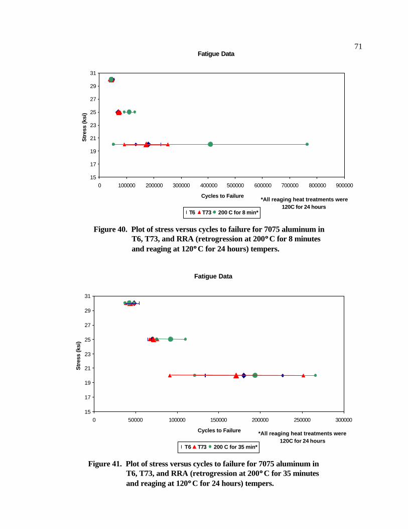
71

Fatigue Data

15

17

19

21

23

25

27

29

31

0 100000 200000 300000 400000 500000 600000 700000 800000 900000

Cycles to Failure

Str

ess

(ksi

)

T6 T73 200 C for 8 min*

*All reaging heat treatments were 120C for 24 hours

Figure 40. Plot of stress versus cycles to failure for 7075 aluminum in T6, T73, and RRA (retrogression at 200°° C for 8 minutes and reaging at 120°° C for 24 hours) tempers.

Fatigue Data

15

17

19

21

23

25

27

29

31

0 50000 100000 150000 200000 250000 300000

Cycles to Failure

Str

ess

(ksi

)

T6 T73 200 C for 35 min*

*All reaging heat treatments were 120C for 24 hours

Figure 41. Plot of stress versus cycles to failure for 7075 aluminum in T6, T73, and RRA (retrogression at 200°° C for 35 minutes and reaging at 120°° C for 24 hours) tempers.

72

The fatigue test results indicate that 7075 aluminum alloy in the RRA temper

performed equal to slightly better than in the T6 and T73 tempers. Due to the fact the

standard deviation bars overlapped, it appears that the fatigue properties in aluminum

7075 are not significantly affected when choosing between the T6, T73, and RRA

tempers evaluated in this research.

4.4 Fracture toughness test results

The fracture toughness results are shown in Table 7. The KIC value, or plain strain

fracture toughness as defined in section 3.7, is based on an average of two tests for each

temper.

The experimentally determined KIC values compare favorably with accepted

values. The results indicate that the fracture toughness of the RRA temper is lower than

the T73 and within 4% of the T6 value.

The relative difference in values of fracture toughness of each of the tempers is

explained theoretically. Aging to obtain the T6 temper increases the yield strength as

TEMPER KIC (ksi in ) T6 21.0 T73 28.8 RRA (RETROGESSED 160°C FOR 660 MIN/ REAGED 120°C FOR 24 HRS)

20.2

RRA (RETROGESSED 180°C FOR 120 MIN/ REAGED 120°C FOR 24 HRS)

20.4

Table 7. Results of fracture toughness tests on 7075 aluminum alloy in the T6, T73, and RRA tempers.

73

described in section 1.2. However, this aging also decreases the both the ductility and

toughness of the material. Overaging decreases the yield strength, but recovers some of

the ductility. Therefore, similar to the trade-off between SCC resistance and strength,

there is a trade-off between strength and fracture toughness when choosing between the

T6 and T73 tempers. The RRA temper has strength levels comparable to the T6 temper

and behaves similar to the T6 temper with respect to fracture toughness values.

4.5 Alternate immersion results

The results of the alternate immersion test are shown in Figures 42-47. The data

are shown as the percentage of yield strength of the material versus days to failure. As

Figure 42. Results of alternate immersion test for 7075 aluminum in T6, T73, and RRA (retrogression at 160°° C for 250 minutes and reaging at 120°° C for 24 hours) tempers.

Alternate Immersion Results

0

10

20

30

40

50

60

70

80

90

100

0 20 40 60 80 100 120 140 160

Days to fai lure

T6 T73 160 C for 250 min

74

detailed in section 3.6, the alternate immersion test is an accelerated means of providing

comparative data of corrosion susceptibility of various materials. Those materials with

higher resistance to SCC will generally have a larger number of days to failure in

alternate immersion. As expected, the T73 temper lasted longer during this experiment.

The arrows indicate that the specimens remained unbroken at the time of this report.

Figure 43. Results of alternate immersion test for 7075 aluminum in T6, T73, and RRA (retrogression at 160°° C for 275 minutes and reaging at 120°° C for 24 hours) tempers.

Alternate Immersion Results

0

10

20

30

40

50

60

70

80

90

100

0 20 40 60 80 100 120 140 160

Days to Fa i lure

T6 T73 160 C for 275 min

75

Figure 44. Results of alternate immersion test for 7075 aluminum in T6, T73, and RRA (retrogression at 180°° C for 35 minutes and reaging at 120°° C for 24 hours) tempers.

Alternate Immersion Results

0

10

20

30

40

50

60

70

80

90

100

0 20 40 60 80 100 120 140 160

Days to Failure

Per

cen

tag

e o

f Yie

ld S

tren

gth

T6 T73 180 C for 35 min

Figure 45. Results of alternate immersion test for 7075 aluminum in T6, T73, and RRA (retrogression at 180°° C for 50 minutes and reaging at 120°° C for 24 hours) tempers.

Alternate Immersion Data

0

10

20

30

40

50

60

70

80

90

100

0 20 40 60 80 100 120 140 160

Days to Failure

Per

cent

age

of Y

ield

Str

engt

h

T6 T73 180 C for 50 min

76

Alternate Immersion Results

0

1 0

2 0

3 0

4 0

5 0

6 0

7 0

8 0

9 0

1 0 0

0 2 0 4 0 6 0 8 0 1 0 0 1 2 0 1 4 0 1 6 0

Days to Failure

Per

ecnt

age

of Y

ield

Str

engt

h

T6 T73 200 C for 8 min

Figure 46. Results of alternate immersion test for 7075 aluminum in T6, T73, and RRA (retrogression at 200°° C for 8 minutes and reaging at 120°° C for 24 hours) tempers.

Alternate Immersion Results

0

1 0

2 0

3 0

4 0

5 0

6 0

7 0

8 0

9 0

1 0 0

0 2 0 4 0 6 0 8 0 1 0 0 1 2 0 1 4 0 1 6 0

Days to Failure

Per

cent

age

of Y

ield

Str

engt

h

T6 T73 200 C for 35 min

Figure 47. Results of alternate immersion test for 7075 aluminum in T6, T73, and RRA (retrogression at 200°° C for 35 minutes and reaging at 120°° C for 24 hours) tempers.

77

The results of the alternate immersion experiment indicate that the RRA tempers

behaved in a similar manner to that of the T6 temper for aluminum alloy 7075. In other

words, the experimentation indicated that there was no significant change in the time to

failure as measured through alternate immersion testing. Therefore, the RRA tempers did

not exhibit improvement in resistance to SCC as compared to the T6 temper.

4.6 Double-cantilever beam results

DCB testing was conducted to evaluate the SCC behavior of a material in the

presence of a flaw. Furthermore, the test is useful in determining the Stage II crack

growth rate of a material when it is subjected to a corrosive environment. Data from a

double-cantilever experiment are typically shown as the crack growth rate (da/dt) versus

stress intensity (K) as described in section 3.9. The results from the DCB

experimentation in this work are shown in Figures 48-50.

78

DCB Results

1.00E-05

1.00E-04

1.00E-03

1.00E-02

1.00E-01

0 5 10 15 20 25 30 35

Stress Intensity (ksi*in^.5)

Cra

ck G

row

th R

ate

(in/h

r)

T73 T6 160 C for 250 min 160 C for 275 min

Figure 48. Crack growth rate versus stress intensity plot for 7075 aluminum in T6, T73, RRA (retrogression at 160°° C for 250 minutes and reaging at 120°° C for 24 hours), RRA (retrogression at 160°° C for 275 minutes and reaging at 120°° C for 24 hours) tempers.

79

DCB Results

1.00E-05

1.00E-04

1.00E-03

1.00E-02

1.00E-01

0 5 10 15 20 25 30 35

Stress Intensity (ksi*in^.5)

Cra

ck G

row

th R

ate

(in/h

r)

T73 T6 180 C for 35 min 180 C for 50 min

Figure 49. Crack growth rate versus stress intensity plot for 7075 aluminum in T6, T73, RRA (retrogression at 180°° C for 35 minutes and reaging at 120°° C for 24 hours), RRA (retrogression at 180°° C for 50 minutes and reaging at 120°° C for 24 hours) tempers.

80

DCB Results

1.00E-05

1.00E-04

1.00E-03

1.00E-02

1.00E-01

0 5 10 15 20 25 30 35

Stress Intensity (ksi*in^.5)

Cra

ck G

row

th R

ate

(in/h

r)

T73 T6 200 C for 35 min 200 C for 8 min

Figure 50. Crack growth rate versus stress intensity plot for 7075 aluminum in T6, T73, RRA (retrogression at 200°° C for 8 minutes and reaging at 120°° C for 24 hours), RRA (retrogression at 200°° C for 35 minutes and reaging at 120°° C for 24 hours) tempers.

81

The results of the DCB experiment indicate that the RRA temper exhibited

slightly lower crack growth rates than that of the T6 temper. However, the crack growth

rates of the RRA temper were still much higher than that that of the T73 temper.

Generally, materials with better resistance to SCC will exhibit lower crack growth rates.

Therefore, there was only a slight improvement in SCC resistance with each of the RRA

tempers.

82

5.0 FOLLOW-ON EXPERIMENTATION

The results of the initial testing indicate that the selected RRA heat treatments

exhibited similar to slightly better corrosion properties compared to the T6 temper. It

was determined that the chosen retrogression times were not long enough to display

significant improvement and as a result, further modifications to the RRA temper were

made for additional testing.

5.1 Conductivity and hardness measurements

Since conductivity can be related to SCC resistance, conductivity measurements

were used to select RRA times for the second phase of testing. Samples were

retrogressed at 160°C and 180°C for various times. The conductivity and hardness of

each of the samples were measured. The results of the experimentation are shown in

Table 7. In order to get a better representation of Table 7, Figures 51 and 52 display the

hardness versus conductivity for each measured temper of 7075 aluminum. Based on

these measurements, two more RRA combinations were chosen for additional corrosion

testing. These two heat treatments, given in Table 8, maintain hardness (strength) while

maximizing conductivity values.

83

TEMPER CONDUCTIVITY (%IACS)

HARDNESS (HRB)

RRA (RETRO 160°C FOR 250 MINUTES/ REAGED 120°C FOR 24 HOURS)

35.0 88.2

RRA (RETRO 160°C FOR 275 MINUTES/ REAGED 120°C FOR 24 HOURS)

35.0 88.1

RRA (RETRO 160°C FOR 360 MINUTES/ REAGED 120°C FOR 24 HOURS)

35.0 87.7

RRA (RETRO 160°C FOR 420 MINUTES / REAGED 120°C FOR 24 HOURS)

36.7 84.6

RRA (RETRO 160°C FOR 480 MINUTES / REAGED 120°C FOR 24 HOURS)

36.7 86.5

RRA (RETRO 160°C FOR 540 MINUTES / REAGED 120°C FOR 24 HOURS)

36.7 84.1

RRA (RETRO 160°C FOR 660 MINUTES / REAGED 120°C FOR 24 HOURS)

38.2 86.6

RRA (RETRO 160°C FOR 720 MINUTES / REAGED 120°C FOR 24 HOURS)

38.2 85.5

RRA (RETRO 180°C FOR 120 MINUTES / REAGED 120°C FOR 24 HOURS)

38.7 86.4

RRA (RETRO 180°C FOR 180 MINUTES / REAGED 120°C FOR 24 HOURS)

39.4 82.3

RRA (RETRO 180°C FOR 240 MINUTES / REAGED 120°C FOR 24 HOURS)

39.4

78.2

RRA (RETRO 180°C FOR 300 MINUTES / REAGED 120°C FOR 24 HOURS)

42.5 80.4

RRA (RETRO 180°C FOR 360 MINUTES / REAGED 120°C FOR 24 HOURS)

43.3 81.0

T6 34.2 86.85

T73 39.8 81.77

Table 7. Conductivity and hardness measurements for various tempers of aluminum 7075.

84

8 1

8 2

8 3

8 4

8 5

8 6

8 7

8 8

8 9

3 0 3 2 3 4 3 6 3 8 4 0 4 2

Conductivity (%IACS)

Har

dnes

s (H

RB

)

RRA @ 160 C T6 T73

160 C/ 420 MIN

160 C / 250 MIN

160 C/ 520MIN

160 C/ 660 MIN

160 C / 275 MIN

160 C / 360 MIN

160 C/ 480 MIN

160 C/ 720 MIN

T73

T6

Figure 51. Plot of HRB versus conductivity for 7075 aluminum in T6, T73, and various RRA tempers (retrogression @ 160°° C).

7 7

7 9

8 1

8 3

8 5

8 7

8 9

3 0 3 2 3 4 3 6 3 8 4 0 4 2 4 4

Conductivity (% IACS)

Har

dnes

s (H

RB

)

RRA @ 180 T6 T73

180 C / 180 MIN

180 C / 120 MIN

180 C / 300 MIN

180 C / 240 MIN

T6

T73 180 C / 360 MIN

Figure 52. Plot of HRB versus conductivity for 7075 aluminum in T6, T73, and various RRA tempers (retrogression @ 180°° C).

85

5.2 Alternate Immersion results from follow-on experimentation

A second set of alternate immersion tests were conducted at ALCOA Technical

Center. The alternate immersion results for the follow-on experimentation are shown in

Figures 53 and 54. The data are shown as the percentage of yield strength versus the

Retrogression Temp (°° C)

Retrogression Time (min)

Reaging Temp (°° C)

Reaging Time (hours)

160 660 120 24 180 120 120 24

Table 8. Retrogression and reaging (RRA) heat treatments chosen for continued experimentation

Alternate Immersion Results

0

1 0

2 0

3 0

4 0

5 0

6 0

7 0

8 0

9 0

1 0 0

0 2 0 4 0 6 0 8 0 1 0 0 1 2 0 1 4 0 1 6 0

Days to Failure

Per

cent

age

of Y

ield

Str

engt

h

T6 T73 160 C for 660 min

Figure 53. Results of alternate immersion test for 7075 aluminum in T6, T73, and RRA (retrogression at 160°° C for 660 minutes and reaging at 120°° C for 24 hours) tempers.

86

number of days until failure in alternate immersion. The arrows on the data points

indicate that the specimens had not failed at the time of this report.

The results of the alternate immersion indicate that the new RRA tempers

performed better than the previous RRA tempers and the T6 temper. The new tempers

were unbroken through 21 days of testing indicating improved SCC resistance.

Figure 54. Results of alternate immersion test for 7075 aluminum in T6, T73, and RRA (retrogression at 180°° C for 120 minutes and reaging at 120°° C for 24 hours) tempers.

Alternate Immersion Results

0

10

20

30

40

50

60

70

80

90

100

0 20 40 60 80 100 120 140 160

Days to Fa i lure

T6 T73 180 C for 120 min

87

5.3 Double-cantilever beam results from follow-on experimentation

The results of the DCB experiment for the follow-on RRA heat treatments are

shown in Figure 55. As mentioned previously, the DCB data provides critical

information about the crack growth response of a material exposed to a corrosive

environment.

Figure 55. Crack growth rate versus stress intensity plot for 7075 aluminum in T6, T73, and RRA (retrogression at 160°° C for 660 minutes and reaging at 120°° C for 24 hours/retrogression at 180°° Cfor 120 minutes and reaging at 120°° C for 24 hours) tempers.

DCB Data

1.00E-05

1.00E-04

1.00E-03

1.00E-02

1.00E-01

0 5 10 15 20 25 30 35

Stress Intensity (ksi*in^.5)

Cra

ck G

row

th R

ate

(in/h

r)

T6 RRA (160 C FOR 660 MIN) RRA (180 C FOR 120 MIN) T73

88

The DCB results indicate that the RRA temper using a retrogression temperature

of 160°C and retrogression time of 660 minutes produced substantially lower crack

growth rates than that of the T6 temper. The RRA temper using a retrogression

temperature of 180°C and retrogression time of 120 minutes produced only slightly lower

crack growth rates. Therefore, it appears that the RRA tempers showed improvement in

SCC resistance compared to the T6 temper.

The data indicates that for the RRA temper with retrogression at 160°C there are

lower crack growth rates at high stress intensities. This scatter in the data is often seen in

the DCB experimentation due to the numerous variables involved in characterizing stress

corrosion cracking.

89

6.0 DISCUSSION

6.1 Stress Corrosion Cracking Behavior and Fractography

For comparison, Figure 56 shows all of the tempers investigated in this research

plotted as yield strength versus the average stage II crack growth rate. In general, the

various RRA tempers produce strengths similar to that of T6 with lower crack growth

rates. The RRA temper with retrogression at 160°C for 660 minutes produced the

greatest improvement, with only a 4% reduction in strength below T6.

Figure 56. Plot of 0.2% yield stress versus crack growth rate for 7075aluminum in T6, T73, and various RRA tempers.

0.2% Yield Stress vs Crack Growth Rate

56

57

58

59

60

61

62

63

64

65

66

0.00E+00 1.00E-04 2.00E-04 3.00E-04 4.00E-04 5.00E-04 6.00E-04 7.00E-04 8.00E-04 9.00E-04 1.00E-03

Crack Growth Rate (in/hr)

0.2%

Yie

ld S

tres

s

RRA (11 HOURS/ 160) RRA (2 HOURS/ 180 C)

RRA (35 MINUTES/ 200 C)

RRA (275 MINUTES/ 160 C)

RRA (250 MINUTES/ 160 C)

RRA (50 MINUTES/ 180 C)

RRA (8 MINUTES/ 200 C)

RRA (35 MINUTES/ 180 C)

T73

T6

90

Figure 56 also indicates that the trade-off between the T6 and T73 tempers is

reduced with the use of the RRA tempers. For a given yield strength, the crack growth

rate is lower with the use of this temper.

Figures 57, 58, and 59 show scanning electron microscope (SEM) micrographs of

1 mm

Figure 57a. SEM micrograph of 7075 aluminum in the T6 temper broken in laboratory air.

91

the characteristic fracture surfaces of 7075 T6, 7075 RRA, and 7075 T73, respectively.

The fracture surfaces in these micrographs indicate that the material increases in ductility

with increasing aging time. In other words, T6 is the least ductile and T73 is the most

ductile. Improvement as a function of temper is evident with the increase in number and

100 µm

Figure 57b. SEM micrograph of 7075 aluminum in the T6 temper broken in laboratory air (Higher magnification of an area on Figure 57a).

92

subsequent decrease in size of the ductile fracture sites.

1 mm

Figure 58a. SEM micrograph of 7075 aluminum retrogressed at 160°° C for 660 minutes and reaged at 120°° C for 24 hours broken in laboratory air.

93

100 µm

Figure 58b. SEM micrograph of 7075 aluminum retrogressed at 160°° C for 660 minutes and reaged at 120°° C for 24 hours broken in laboratory air (Higher magnification of an area on Figure 58a).

94

1 mm

Figure 59a. SEM micrograph of 7075 aluminum in the T73 temper broken in laboratory air.

95

100µm

Figure 59b. SEM micrograph of 7075 aluminum in the T73 temper broken in laboratory air (Higher magnification of an area on Figure 59a).

96

Figure 60 shows an SEM micrograph of 7075 T6 aluminum exposed to 3.5 %

NaCl through alternate immersion. The transition from stress corrosion cracking to

ductile overload is evident and indicated by the blue lines. The fracture surface of the

1 mm

Figure 60a. SEM micrograph of 7075 aluminum in the T6 temper exposed to 3.5% NaCl by alternate immersion.

97

ductile overload region in Figure 60 is similar to the fracture surface shown in Figure 58.

100 µm

Figure 60b. SEM photograph of 7075 aluminum in the T6 temper exposed to 3.5% NaCl through alternate immersion (Higher magnification of an area on Figure 60a).

98

6.2 Heat Transfer Analysis

A heat transfer analysis for the thermal treatment of aluminum 7075 was

performed in this work for two major reasons. The first reason is to justify why the RRA

heat treatment that Cina proposed in 1974 is only appropriate to thin sections of material.

The second reason is to provide a realistic model as to the limitations of the RRA heat

treatment on thicker sections of material. The important issue in the heat treatment

process is the time for the material to reach the intended temperature, which is equal to

the furnace temperature.

All of the following calculations are analyzed using a constant thickness plate.

Consider a slab of thickness 2L at an initial temperature, Ti, both sides of which are

exposed suddenly to a medium of temperature T (A schematic is shown in Figure 61).

The heat transfer coefficient, h, is assumed to be equal on both sides of the plate. For

unidirectional conduction, the temperature distribution of the material is assumed to

depend only on the x direction and time, t. The excess temperature function is given by:

θ ( , ) ( , )x t T x t T= − ∞ .

k h, T h, T

-L 0 L x

Figure 61. Plate of thickness 2L immersed in a fluid with a different temperature.

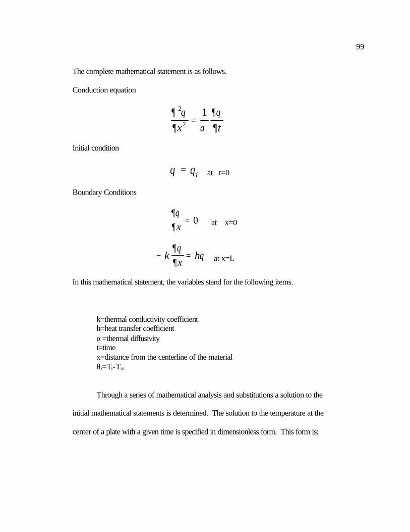
99

The complete mathematical statement is as follows.

Conduction equation

∂ θ∂ α

∂θ∂

2

2

1x t

=

Initial condition

θ θ= i at t=0

Boundary Conditions

∂θ∂ x

= 0 at x=0

− =kx

h∂θ∂

θ at x=L

In this mathematical statement, the variables stand for the following items.

k=thermal conductivity coefficient h=heat transfer coefficient α=thermal diffusivity t=time x=distance from the centerline of the material θi=Ti-T∞

Through a series of mathematical analysis and substitutions a solution to the

initial mathematical statements is determined. The solution to the temperature at the

center of a plate with a given time is specified in dimensionless form. This form is:

100

θθ

( , ) ( , )x t T x t TT Ti i

=−

−∞

∞

The solution is determined graphically through the use of Heisler’s charts. The

chart plots the dimensionless temperature versus the Fourier number. The Fourier

number is defined as follows.

Fot

L=

α2

The various curves on the charts represent the inverse of the Biot (Bi) number, where the

Biot number is defined as follows.

BihLk

=

Given a material with known thermal properties, dimensions and initial

temperature as well as time, heat transfer coefficient and ambient temperature, the

temperature at the center of the block is determinable [34].

In order to make the calculation more realistic, the unidirectional heat conduction

is extended to three dimensions. In this case, the dimensionless temperature is expressed

as the following.

θθ

θθ

θθ

θθ

( , , , ) ( , )*

( , )*

( , )x y z t x t y t z t

i i i i

=

101

This statement shows that the dimensionless temperature for conduction in three

dimensions is the product of the dimensionless temperatures in each of the three different

dimensions.

The heat transfer model is utilized to compare the use of high and low

retrogression temperatures during the RRA process. The high retrogression temperature

heat treatment of 220°C for 5 minutes and the low retrogression temperature heat

treatment of 160°C for 660 minutes were chosen. The 220°C temperature and time has

been shown to produce reduced stage II crack growth rates compared to the T6 temper.

[18]. The 160°C temperature and time was shown to produce favorable strength and

SCC resistance in this research.

Through the use of the Hiesler charts, the temperature of the center of a

rectangular plate is determined. The heat transfer coefficient (h) is estimated to be 100

W/m2K. This is typical value for gases at atmospheric pressure. The thermal diffusivity

(α) of aluminum is 0.667 cm2/s and the thermal conductivity (k) is 167 W/m-K.

Assuming a three-inch cubic block, which is comparable to common aircraft extrusion

thicknesses, the Fourier number is determinable in all three dimensions. The temperature

of the block is assumed to start at 25°C. Table 9 displays theoretical temperature at the

center of a cubic block following the retrogression heat treatment.

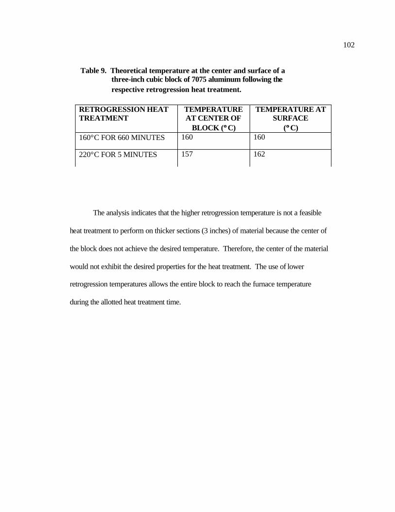
102

The analysis indicates that the higher retrogression temperature is not a feasible

heat treatment to perform on thicker sections (3 inches) of material because the center of

the block does not achieve the desired temperature. Therefore, the center of the material

would not exhibit the desired properties for the heat treatment. The use of lower

retrogression temperatures allows the entire block to reach the furnace temperature

during the allotted heat treatment time.

RETROGRESSION HEAT TREATMENT

TEMPERATURE AT CENTER OF

BLOCK (°° C)

TEMPERATURE AT SURFACE

(°° C) 160°C FOR 660 MINUTES 160 160

220°C FOR 5 MINUTES 157 162

Table 9. Theoretical temperature at the center and surface of a three-inch cubic block of 7075 aluminum following the respective retrogression heat treatment.

103

7.0 CONCLUSIONS

The results of this research indicate that theT6 temper exhibits strengths that are

ten to fifteen percent higher than the T73 temper, but has crack growth rates that are

approximately ten times faster than T73. Furthermore, the T6 temper fails much more

quickly when subjected to 3.5% NaCl in the alternate immersion test.

The RRA temper alleviates the trade-off in properties between these two tempers.

However, the use of a high retrogression temperatures limit the use to thinner sheets of

material. This research proved that lower retrogression temperatures and corresponding

longer retrogression times alleviates the trade-off between the T6 and T73 temper for AA

7075. The improvement in properties is summarized as follows.

• RRA tempers with retrogression temperatures down to 160°C produced crack

growth rates lower than that of the T6 temper during the double-cantilever beam

experiment.

• RRA tempers with retrogression temperatures down to 160°C lasted substantially

longer than T6 in the alternate immersion test.

• Fatigue properties, fracture toughness, and 0.2% yield strength of material in the

RRA temper compare favorably to the T6 temper.

Furthermore, heat transfer analysis and results of the corrosion tests indicate the

RRA temper with lower retrogression is a more viable temper for use in industry. The

longer retrogression times (8-11 hours) allow the temper to be applied to much thicker

sections of material.

104

8.0 RECOMMENDATIONS

The trends of this research indicate that the use of lower retrogression

temperatures and corresponding longer retrogression times are feasible. Additional

testing is warranted to confirm the viability of using the RRA tempers tested in this

research in industry.

Another recommendation is to perform the RRA heat treatment using lower

retrogression temperatures on other aluminum alloys. The chemical compositions of an

alloy and its microstructural properties have a significant effect on tempering response.

Other alloys may produce even better corrosion and strength properties with the use of

the RRA temper.

Furthermore, transmission electron microscopy (TEM) work would help explain

the effect of the microstructural changes on the strength and SCC properties of various

RRA tempers.

105

9.0 APPENDICES

9.1 Tuning Procedure for Muffle Furnace

The operating temperature was set on the furnace. The furnace was loaded with

aluminum blocks (characteristic load for the heat treating). The “SEL” button was

depressed until “AT” displayed. The “AT”, or auto-tune was turned on. The self-tuning

set values for proportional band-P, integral-I, and derivative-d. These three modes allow

the furnace to operate with over-temperature protection and “Fuzzy” logic capability.

These tuning characteristics help to increase the accuracy of the furnace and keep the

internal temperature as constant as possible.

9.2 Fatigue Apparatus Tuning Procedure

The weight that is added to the reciprocating assembly to tune it to the compensator

spring is known as the complementary weight. The factory determines this

complementary weight through calibration. The weight required to tune the system is

called the tuning weight. The sum of the tuning weight and the effective weight must

equal the complementary weight. Effective weight is determined from the type of

specimen to be used for the test. The tuning weight is then added to the apparatus on

both sides of the oscillator. When the proper tuning weight is utilized, the compensator

spring will allow the alternating force applied to the specimen to be equal to that

produced by the oscillator.

106 9.3 Pre-cracking Procedure for Fracture Toughness Testing

Knife edges were mounted on the specimens and were spread 0.2 inches apart. The clip

gage was calibrated and mounted on to the knife edges. The specimens were mounted in

the MTS machine to begin the fatigue pre-cracking. The minimum to maximum load

ratio was between –1 and .1 and the number of cycles to complete the pre-cracking was

between (104) and (106). Furthermore, the maximum stress intensity in the final stages of

the pre-crack must not exceed 60% of the KIC value for the material. The final stage, or

2.5 % stage is the point where the crack has reached 97.5% of its total length.

The final fatigue crack length was between 0.45 and 0.55 W where W is the distance from

the load point to the end of the specimen. W for the compact-tensile specimens was is

two inches. Therefore, the fatigue pre-cracking was set to extend 0.1 inches beyond the

end of the notch in order to meet ASTM requirements. In order to ensure the fatigue pre-

crack was symmetrical, specimens were inverted after 0.05 inches of crack growth. This

helps to compensate for any imbalance in the MTS apparatus and ensure a straight crack

front.

107

9.4 Pre-cracking Procedure for DCB Test

The necessary relationships to perform the pre-cracking were determined in the following

manner.

(1) GPb

dcda

=2

2 (2) K GEP

hahI = = +

120 7( . )

where G=crack extension force c=specimen compliance (reciprocal thickness)

P=load b=specimen thickness a=crack length measured from the load point (centerline of loading bolt) h=half height of DCB specimen

Based on the above equations, the following was derived.

dcGbP

da=2

2

cb

PGda

bP E

K da= = ∫∫2 2

2 22

108

cb

P EP a

da

cb

Ea

da

= +

= +

∫

∫

2 120 5 5

0 7

480 5

0 7

2

2

2

. ..

..

cvP

= (v is deflection of the two arms at the load point)

Thus, the parameter Cc was incorporated to arrive at the following expression.

CEbvP

adac = = +

∫48

050 7

2

..

Cc was plotted versus crack length a, for 0.5<a<1 inch. A fourth order expression was

determined for crack length, a, as a function of the parameter Cc. This expression was

input into the program in order to monitor crack length with an extensometer [35].

109

9.5 Data From Double-Cantilever Beam Experiment

The following chart lists the data taken for one DCB specimen through a testing

period. The data is plotted as the crack rate versus stress intensity.

Length(x) Length (y) Crack Distance from Crack Distance from Avg. Distance from Deflection (in) Stress Intensity Time (hours) Crack rateLoad Line (in) Load Line (in) Load Line (in) (ksi*in^.5) (in/hr)

1.063 1.055 0.688 0.68 0.684 0.017 23.74939616 241.063 1.062 0.688 0.687 0.6875 23.59459545 48 0.0001461.073 1.084 0.698 0.709 0.7035 22.90610216 72 0.0006671.139 1.131 0.764 0.756 0.76 20.70367753 144 0.0007851.159 1.135 0.784 0.76 0.772 20.2772474 168 0.00051.191 1.168 0.816 0.793 0.8045 19.1866993 189 0.0015481.228 1.2 0.853 0.825 0.839 18.1229693 213 0.0014381.302 1.31 0.927 0.935 0.931 15.68371004 288 0.0012271.312 1.333 0.937 0.958 0.9475 15.29866434 312 0.0006871.333 1.368 0.958 0.993 0.9755 14.67689212 355 0.0006511.363 1.41 0.988 1.035 1.0115 13.93150999 403 0.000751.376 1.449 1.001 1.074 1.0375 13.42782519 475 0.0003611.474 1.529 1.099 1.154 1.1265 11.89494114 554 0.0011271.546 1.565 1.171 1.19 1.1805 11.08887268 643 0.0006071.548 1.659 1.173 1.284 1.2285 10.4388504 739 0.00051.597 1.681 1.222 1.306 1.264 9.993964796 811 0.0004931.709 1.777 1.334 1.402 1.368 8.841787016 1003 0.000542

110

10.0 REFERENCES

1. Altenpohl, D., Aluminum: Technology, Applications, and Environment, 6th Edition. Washington D.C.: The Aluminum Association (1998). 2. Smith, W. Principles of Materials Science and Engineering. McGraw-Hill, Inc: New York (1996), p.534. 3. Adler, P., DeIasi, R., Geschwind, G., “Influence of Microstructure on the Mechanical Properties and Stress Corrosion Susceptibility of 7075 Aluminum Alloy,” Metallurgical Transactions V3 (1972), pp. 3191-3200. 4. Hatch, J. Aluminum: Properties and Physical Metallurgy. Ohio: American Society for Metals (1984), pp. 245, 5. Holroyd, N. “Environment-Induced Cracking of High-Strength Aluminum Alloys,” EICM Proceedings, pp.311-343. 6. Lisagor, B., “Environmental Cracking-Stress Corrosion,” Materials Division, NASA Langley Research Center, pp.240-252. 7. Speidel, “State of The Art of Stress-Corrosion Cracking in High-Strength Aluminum Alloys,” (1971), pp.1-63. 8. Hunt, W., Staley, J., “High-Strength Aluminum Alloys for Aerospace Application,” Alcoa Laboratories (1989), pp.111-120. 9. Gerhardus, H., “Stress-Corrosion Cracking and Hydrogen Embrittlement,” CC Technologies, Inc., pp. 493-500. 10. From: http://www.aloha.net/~icarus 11. Kanno, M., Araki, I., Cui, Q., “Precipitation Behavior of 7000 Alloys During Retrogression and Reaging Treatment,” Materials Science and Technology V10 (1994), pp.599-603. 12. Hyatt, M., Speidel, M., “Stress-Corrosion Cracking of Aluminum Alloys,” Work for: Boeing Commercial Airplane Group (1970), pp.185-188. 13. Rajan, K., Wallace, W., Beddoes, J., “Mictrostructural Study of the High-Strength Stress Corrosion Resistant 7075 Aluminum Alloy,” Journal of Materials Science V17 (1982), pp.2817-2824. 14. Park, J.K., Ardell, A.J. “Effect of Retrogression and Reaging Treatments on the Microstructure of Al-7075-T651,” Metallurgical Transactions A, 15A (1984), pp. 1531-1543. 15. Park, J.K. “Influence of Retrogression and Reaging Treatments on the Strength and Stress Corrosion Resistance of Aluminum Alloy 7075-T6,” Materials Science and Engineering, A103 (1988), pp. 223-231. 16. Ural. K., “A Study of Optimization of Heat-Treatment Conditions in Retrogression and Reageing Treatment of 7075-T6 Aluminum Alloy,” Journal of Materials Science Letters V13 (1994), pp.383-385. 17. Fleck, P., Calleros, D., Madsen, M., Trinh, T., Hoang, D., Foyos, J., Lee, E.W., Es-Said, O.S., “Retrogression and Reaging of the 7075 T6 Aluminum Alloy,” NSF Research Experience for Undergraduate Program, Loyola Marymount University, Los Angeles CA, 90045-8145, U.S.A.

111

18. Hyatt, M. “Use of Precracked Specimens in Stress Corrosion Testing of High Strength Aluminum Alloys,” Corrosoin-NACE V26 (1970), pp.487-503. 19. Wallace, W., Beddoes, J., DeMalherbe, M., “A New Approach to the Problem of Stress Corrosion Cracking in 7075-T6 Aluminum,” Canadian Aeronautics and Space Journal V27 (1981), pp. 225-232. 20. Uguz, A., Martin, J. “The Effect of Retrogression and re-ageing on the Ductile Fracture Toughness of Al-Zn-Mg Alloys Containing Different Dispersoid Phases,” Journal of Materials Science V30 (1995), pp. 5923-5926. 21. Thompson, J., Tankins, E., Agarwala, V. “A Heat Treatment for Reducing Corrosion and Stress Corrosion Cracking Susceptibilities in 7xxx Aluminum Alloys,” NACE (1987), pp. 45-51. 22. Robinson, J., Whelan, S., Cudd, R., “Retrogression and Re-ageing of 7010 Open Die Forgings,” Materials Science and Technology V15 (1999), p. 717-724. 23. Mondolfo, L., Aluminum Alloys, Structure and Properties. Butterworths: London (1976). 24. Willey, L., Aluminum 1, ed. K.R. Horn. ASM: Metals Park, Ohio (1967), p.174. 25. Engh, T., Principles of Metal Refining. Oxford University Press (1992). 26. Smith, W. Principles of Materials Science and Engineering. McGraw-Hill, Inc: New York (1996), pp. 130-135. 27. ASTM Standard B557M-94 “Standard Test Methods of Tension Testing Wrought and Cast Aluminum and Magnesium Alloy Product” 28. Holman, J., Experiment Methods for Engineers. McGraw-Hill, Inc.: New York (1994), 58-91. 29. ASTM E399 “Standard Test Method for Plane-Strain Fracture Toughness of Metallic Materials” 30. ASTM G44 “Standard Practice for Evaluating Stress Corrosion Cracking Resistance of Metals and Alloys by Alternate Immersion in 3.5% Sodium Chloride Solution” 31. ASTM E1681-95 “Standard Test Method for Determining a Threshold Stress Intensity Factor for Environment-Assisted Cracking of Metallic Materials Under Constant Load” 32. Mostovoy, S., Crosley, P., Ripling, E., “Use of Crack-Line Loaded Specimens for Measuring Plane-Strain Fracture Toughness,” Journal of Materials (1967), pp.661-670. 33. Jones, G., Laughton, M., Electrical Engineer’s Reference Book 15th Ed. Butterworth Heinemann Ltd. (1993). 34. Bejan, Adrian. Heat Transfer. John Wiley & Sons, Inc: New York (1993), pp.143-177. 35. Sprawley, J., Gross, B., “Stress Intensity Factors for Crackline-Loaded Edge-Crack Specimens,” NASA TN D-3820 (1967), pp. 2-36.