Optimizing Symbolic Model Checking forConstraint-Rich Models

Bwolen Yang Reid Simmons Randal E. BryantDavid R. O’Hallaron

March 1999CMU-CS-99-118

School of Computer ScienceCarnegie Mellon University

Pittsburgh, PA 15213

A condensed version of this technical report will appear in Proceedings ofthe International Conference on Computer-Aided Verification, Trento, Italy(July 1999).

Effort sponsored in part by the Advanced Research Projects Agency and Rome Laboratory,Air Force Materiel Command, USAF, under agreement number F30602-96-1-0287, in part by theNational Science Foundation under Grant CMS-9318163, and in part by grants from the Intel Cor-poration and NASA Ames Research Center. The U.S. Government is authorized to reproduce anddistribute reprints for Governmental purposes notwithstanding any copyright annotation thereon. Theviews and conclusions contained herein are those of the author and should not be interpreted as neces-sarily representing the official policies or endorsements,either expressed or implied, of the AdvancedResearch Projects Agency, Rome Laboratory, or the U.S. Government.

Keywords: symbolic model checking, Binary Decision Diagram (BDD), time-invariant constraints, redundant state-variable elimination, macro.

Abstract

This paper presents optimizations for verifying systems with complex time-invariant constraints. These constraints arise naturally from modeling physicalsystems, e.g., in establishing the relationship between different components in asystem. To verify constraint-rich systems, we propose two new optimizations.The first optimization is a simple, yet powerful, extension of the conjunctive-partitioning algorithm. The second is a collection of BDD-based macro-extractionand macro-expansion algorithms to remove state variables. We show that these twooptimizations are essential in verifying constraint-rich problems; in particular, thiswork has enabled the verification of fault diagnosis models of the Nomad robot (anAntarctic meteorite explorer) and of the NASA Deep Space One spacecraft.

1 IntroductionThis paper presents techniques for using symbolic model checking to automaticallyverify a class of real-world applications that have many time-invariant constraints.An example of constraint-rich systems is the symbolic models developed by NASAfor on-line fault diagnosis[16]. These models describe the operation of compo-nents in complex electro-mechanical systems, such as autonomous spacecraft orrobot explorers. The models consist of interconnected components (e.g., thrusters,sensors, motors, computers, and valves) and describe how themodeof each com-ponent changes over time. Based on these models, the Livingstone diagnostic en-gine[16] monitors sensor values and detects, diagnoses, and tries to recover frominconsistencies between the observed sensor values and the predicted modes of thecomponents. The relationships between the modes and sensor values are encodedusing symbolic constraints. Constraints between state variables are also used toencode interconnections between components. We have developed an automatictranslator from such fault models to SMV (Symbolic Model Verifier)[11], wheremode transitions are encoded as transition relations and state-variable constraintsare translated into sets of time-invariant constraints.

To verify constraint-rich systems, we introduce two new optimizations. Thefirst optimization is a simple extension of the conjunctive-partitioning algorithm.The other is a collection of BDD-based macro-extraction and macro-expansionalgorithms to remove redundant state variables. We show that these two optimiza-tions are essential in verifying constraint-rich problems. In particular, these opti-mizations have enabled the verification of fault diagnosis models for the Nomadrobot (an Antarctic meteorite explorer)[1] and the NASA Deep Space One (DS1)spacecraft[2]. These models can be quite large, with up to 1200 state bits.

The rest of this paper is organized as follows. We first briefly describe symbolicmodel checking and how time-invariant constraints arise naturally from modeling(Section 2). We then present our new optimizations: an extension to conjunctivepartitioning (Section 3), and BDD-based algorithms for eliminating redundant statevariables (Section 4). We then show the results of a performance evaluation on theeffects of each optimization (Section 5). Finally, we present a comparison to priorwork (Section 6) and some concluding remarks (Section 7).

2 Background

Symbolic model checking[5, 7, 11] is a fully automatic verification paradigm thatchecks temporal properties (e.g., safety, liveness, fairness, etc.) of finite state sys-tems by symbolic state traversal. The core enabling technology for symbolic modelchecking is the use of the Binary Decision Diagram (BDD) representation[4] for

1

state sets and state transitions. BDDs represent Boolean formulas canonically asdirected acyclic graphs such that equivalent sub-formulas are uniquely representedas a single subgraph. This uniqueness property makes BDDs compact and enablesdynamic programming to be used for computing Boolean operations symbolically.

To use BDDs in model checking, we need to map sets of states, state transitions,and state traversal to the Boolean domain. In this section, we briefly describethis mapping and motivate how time-invariant constraints arise. We finish withdefinitions of some additional terminology to be used in the rest of the paper.

2.1 Representing State Sets and Transitions

In the symbolic model checking of finite state systems, a state typically describesthe values of many components (e.g., latches in digital circuits) and each compo-nent is represented by astate variable. Let V = fv1; :::; vng be the set of statevariables in a system, then a state can be described by assigning values to all thevariables inV . This valuation can in term be written as a Boolean formula that istrue exactly for the valuation as

Vni=0(vi == ci), whereci is the value assigned to

the variablevi, and the “==” represents the equality operator in a predicate (similarto the C programming language). A set of states can be represented as a disjunctionof the Boolean formulas that represent the states. We denote the BDD representa-tion for a set of statesS by S(V ).

In addition to the set of states, we also need to map the system’s state transitionsto the Boolean domain. We extend the above concept of representing a set of statesto representing a set of ordered-pairs of states. To represent a pair of states, weneed two sets of state variables:V the set ofpresent-state variablesfor the firsttuple andV 0 the set ofnext-state variablesfor the second tuple. Each variablev inV has a corresponding next-state variablev0 in V 0. A valuation of variables inVandV 0 can be viewed as a state transition from one state to another. A transitionrelation can then be represented as a set of these valuations. We denote the BDDrepresentation of a transition relationT asT (V; V 0).

In modeling finite state systems, the overall state transitions are generally spec-ified by defining the valid transitions for each state variable. To support non-deterministic transitions of a state variable, the expression that defines the tran-sitions evaluates to a set, and the next-state value of the state variable is non-deterministically chosen from the elements in the set. Hereafter, we refer to anexpression that evaluates to a set either as aset expressionor as anon-deterministicexpressiondepending on the context, and we use the bold font type, as inf, to rep-resent such expression. Letfi be the set expression representing state transitionsof the state variablevi. Then the BDD representation forvi’s transition relationTi

2

can be defined asTi(V; V

0) := (v0i 2 fi(V )):

For synchronous systems, the BDD for the overall state transition relationT is

T (V; V 0) :=

n̂

i=0

Ti(V; V0):

Detailed descriptions on this formulation, including mapping of asynchronous sys-tems, can be found in[5, 11].

Note that in the above formulation, we also need to represent non-Booleanexpressions (such asfi’s) or non-Boolean variables as part of intermediate step.These non-Boolean formulas can be represented using variants of BDDs (e.g.,MTBDD [6]) that extend the BDD concept to include non-Boolean values. Theseextensions also include algorithms for Boolean operators with non-Boolean argu-ments like the “==” and “2”. We will refer to all these BDD-variants simply asBDDs.

2.2 Time-Invariant Constraints and Their Common Usages

In symbolic model checking, time-invariant constraints specify the conditions thatmust always hold. More formally, letC1, . . . ,Cl be the time-invariant constraintsand letC := C1 ^ C2 ^ ::: ^ Cl. Then, in symbolic state traversal, we consideronly states whereC is true. We refer toC as theconstrained space.

To motivate how time-invariant constraints arise naturally in modeling complexsystems, we describe three common usages. One common usage is to make thesame non-deterministic choice across multiple expressions in transition relations.For example, in a master-slave model, the master can non-deterministically choosewhich set of idle slaves to assign the pending jobs, and the slaves’ next-state valueswill depend on the choice made. To model this, letf be the non-deterministicexpression representing how the master makes its choice. If the slaves’ transitionrelations are defined using the expressionf directly, then each use off makes itsown non-deterministicchoice independent of other uses. Thus, to ensure that all theslaves see the same non-deterministicchoice, a new state variableu is introduced torecord the choice made, andu is then used to define the slaves’ transition relations.This recording process is expressed as the time-invariant constraintu 2 f.

Another common usage is for establishing the interface between different com-ponents in a system. For example, suppose two components are connected with apipe of a fixed capacity. Then, the input of one component is the minimum of thepipe’s capacity and the output of the other component. This relationship is de-scribed as a time-invariant constraint between the input and the output of these twocomponents.

3

Third common usage is specific uses of generic parts. For example, a bi-directional fuel pipe may be used to connect two components. If we want to makesure the fuel flows only one way, we need to constrain the valves in the fuel pipe.These constraints are specified as time-invariant constraints. In general, specificuses of generic parts arise naturally in both the software and the hardware domainas we often use generic building blocks in constructing a complex system.

In the examples above, the use of time-invariant constraints is not always nec-essary because some these constraints can be directly expressed as a part of thetransition relation and the associated state variables can be removed. However,these constraints are used to facilitate the description of the system or to reflect theway complex systems are built. Without these constraints, multiple expressionswill need to be combined into possibly a very complicated expression. Perform-ing this transformation manually can be labor intensive and error-prone. Thus itis up to the verification tool to automatically perform these transformations andremove unnecessary state variables. Our optimizations for constraint-rich modelsis to automatically eliminate redundant state variables (Section 4) and partition theremaining constraints (Section 3).

2.3 Symbolic State Traversal

To reason about temporal properties, thepre-imageand theimageof the transitionrelation are used for symbolic state traversal, and time-invariant constraints areused to restrict the valid state space. Based on the BDD representations of a statesetS and the transition relationT , we can compute thepre-imageand theimageof S, while restricting the computations to the constrained spaceC, as follows:

pre-image(S)(V ) := C(V ) ^ 9V 0:[T (V; V 0) ^ (S(V 0)^ C(V 0))] (1)

image(S)(V 0) := C(V 0) ^ 9V:[T (V;V 0) ^ (S(V ) ^ C(V ))] (2)

One limitation of the BDD representation is that the monolithic BDD for thetransition relationT is often too large to build. A solution to this problem is theconjunctive partitioning[5] of the transition relation. In conjunctive partitioning,the transition relation is represented as a conjunctionP1 ^ P2 ^ :::^ Pk with eachconjunctPi represented by a BDD. Then, the pre-image can be computed by con-juncting with onePi at a time, and by usingearly quantificationto quantify outvariables as soon as possible. The early-quantification optimization is based on theproperty that sub-formulas can be moved out of the scope of an existential quan-tification if they do not depend on any of the variables being quantified. Formally,letV 0i , a subset ofV 0, be the set of variables that do not appear in any of the subse-quentPj ’s, where1 � i � k andi < j � k. Then the pre-image can be computed

4

as

p1 := 9V 01:[P1(V; V

0) ^ (S(V 0)^ C(V 0))] (3)

p2 := 9V 02:[P2(V; V

0) ^ p1]

...

pk := 9V 0k :[Pk(V; V0) ^ pk�1]

pre-image(S)(V ) := C(V ) ^ pk

The determination and ordering of partitions (thePi’s in above) can have sig-nificant performance impact. Commonly used heuristics[8, 12] treat the state vari-ables’ transition relations (Ti’s) as the partitions. The ordering step then greedilyschedules the partitions to quantify out more variables as soon as possible, whileintroducing fewer new variables. Finally, the ordered partitions are tentativelymerged with their predecessors to reduce the number of intermediate results. Eachmerged result is kept only if the resulting graph size is less than a pre-determinedlimit.

The conjunctive partitioning for the image computation is performed similarlywith present-state variables inV being the quantifying variables instead of next-state variables inV 0. However, since the quantifying variables are different be-tween the image and the pre-image computation, the resulting conjuncts for imagecomputation is typically very different from those for pre-image computation.

2.4 Additional Terminology

We define thesupport variablesof a function to be the variables that the functiondepends on, and thesupportof a function to be the set of support variables. Wedefine theITE operator (if-then-else) as follows: given arbitrary expressionsf andg wheref andg may both be set expressions, and Boolean expressionp, then

ITE(p; f; g)(X) :=

�f(X) if p(X);

g(X) otherwise;

whereX is the set of variables used in expressionsp, f , andg. We define acare-space optimizationas any algorithmcare-optthat has following properties: givenan arbitrary expressionf wheref may be a set expression, and a Boolean formulac, then

care-opt(f; c) := ITE(c; f; d);

whered is defined by the particular algorithm used. The usual interpretation of thisis that we onlycareabout the values off whenc is true. We will refer toc as the

5

care spaceand:c as thedon’t-care space. The goal of care-space optimizationsis to heuristically minimize the representation forf by choosing a suitabled inthe don’t-care space. Descriptions and a study of some care-space optimizations,including the commonly usedrestrictalgorithm[7], can be found in[14].

3 Extended Conjunctive Partitioning

The first optimization is the application of the conjunctive-partitioning algorithmon the time-invariant constraints. This extension is derived based on two obser-vations. First, as with the transition relations, the BDD representation for time-invariant constraints can be too large to be represented as a monolithic graph. Thus,it is crucial to represent the constraints as a set of conjuncts rather than a monolithicgraph.

Second, in constraint-rich models, manyquantifying variables(variables be-ing quantified) do not appear in the transition relation. There are two commoncauses for this. First, when time-invariant constraints are used to make the samenon-deterministic choices, new variables are introduced to record these choices(described as the first example in Section 2.2). In the transition relation, thesenew variables are used only in their present-state form. Thus, their correspondingnext-state variables do not appear in the transition relation, and for the pre-imagecomputation, these next-state variables are parts of the quantifying variables. Theother cause is that many state variables are used only to establish time-invariantconstraints. Thus, both the present- and the next-state version of these variables donot appear in the transition relations.

Based on this observation, we can improve the early-quantification optimiza-tion by pulling out the quantifying variables (V 0

0) that do not appear in any of

the transition relations. Then, these quantifying variables (V 00) can be used for

early quantification in conjunctive partitioning of the constrained space (C) wherethe time-invariant constraints hold. Formally, letQ1; Q2; :::; Qm be the parti-tions produced by the conjunctive partitioning of the constrained spaceC, whereC = Q1 ^ Q2 ^ ::: ^ Qm. For the pre-image computation, Equation 3 is replacedby

q1 := 9W 01:[Q1(V

0)^ S(V 0)]

q2 := 9W 02:[Q2(V

0)^ q1]

...

qm := 9W 0m:[Qm(V 0) ^ qm�1]

p1 := 9V 01:[P1(V; V

0) ^ qm]

6

whereW 0i , a subset ofV 00, is the set of variables that do not appear in any of the

subsequentQj ’s, where1 � i � m andi < j � m. Similarly, this extension alsoapplies to the image computation.

4 Elimination of Redundant State Variables

Our second optimization for constraint-rich models is targeted at reducing the statespace by removing unnecessary state variables. This optimization is a set of BDD-based algorithms that compute an equivalent expression for each variable used inthe time-invariant constraints (macro extraction) and then globally replace a suit-able subset of variables with their equivalent expressions (macro expansion) toreduce the total number of variables.

The use of macros is traditionally supported by language constructs (e.g., DE-FINE in the SMV language[11]) and by simple syntactic analyses such as detectingdeterministic assignments (e.g.,a == f wherea is a state variable andf is an ex-pression) in the specifications. However, in constraint-rich models, the constraintsare often specified in a more complex manner such asconditionaldependencies onother state variables (e.g.,p) (a == f) as conditional assignment of expressionf to variablea whenp is true). To identify the set of valid macros in such models,we need to combine the effects of multiple constraints. One drawback of syntacticanalysis is that, for each type of expression, syntactic analysis will need to adda template to pattern match these expressions. Another more severe drawback isthat it is difficult for syntactic analysis to estimate the actual cost of instantiating amacro. Estimating this cost is important because reducing the number of variablesby macro expansion can sometimes result in significant performance degradationcaused by large increases in other BDD sizes. These two drawbacks make thesyntactic approach unsuitable for models with complex time-invariant constraints.

Our approach uses BDD-based algorithms to analyze time-invariant constraintsand to derive the set of possible macros. The core algorithm is a new assignment-extraction algorithm that extracts assignments from arbitrary Boolean expressions(Section 4.1). For each variable, by extracting its assignment form, we can de-termine the variable’s corresponding equivalent expression, and when appropri-ate, globally replace the variable with its equivalent expression (Section 4.2). Thestrength of this algorithm is that by using BDDs, the cost of macro expansion can bebetter characterized because the actual model checking computation is performedusing BDDs.

Note that there have been a number of research efforts on BDD-based redun-dant state-variable removal. To better compare our approach to these previous re-search efforts, we postpone the discussion of this prior work until Section 6, after

7

describing our algorithms and the performance evaluation.

4.1 BDD-Based Assignment Extraction

The assignment-extraction problem can be stated as follows: given an arbitraryBoolean formulaf and a variablev (wherev can be non-Boolean), findg andhsuch that

� f = (v 2 g) ^ h,

� g does not depend onv, and

� h is a Boolean formula and does not depend onv.

The expression(v 2 g) represents a non-deterministic assignment to variablev.In the case thatg always evaluates to a singleton set, the assignment(v 2 g) isdeterministic. A solution to this assignment-extraction problem is as follows:

h = 9v:f

t =[

k2Kv

ITE(f jv k ; fkg; ;)

g = restrict(t; h)

whereKv is the set of all possible values of variablev, andrestrict [7] is a care-space optimization algorithm that tries to reduce the BDD graph size (oft) bycollapsing the don’t-care space (:h). The BDD algorithm for the

Sk2Kv

operatoris similar to the BDD algorithm for the existential quantification with the_ oper-ator replaced by the[ operator for variable quantification. A correctness proof ofthis algorithm is included in Appendix A.

Currently, we do not have any optimality guarantees for this solution. We doknow that the solutiong doesnot always have the minimum number of supportvariables. i.e.,g is not necessary aminimum-supportsolution. However, based onthe behavior of therestrictalgorithm, we have formed a conjecture about the rela-tionship betweeng and any minimum-support solution. Informally, this conjecturestates thatg can be converted to any minimum-support solution via a sequence ofvariable substitutions, and that these substitutions are parts of equality decomposi-tion of h. More formally,

Conjecture 1 Let gmin be a solution with the minimum number of support vari-ables. Then, there exists a sequence ofn substitutions(ui ei) whereui’s arevariables,ei’s are expressions, and1 � i � n, such that

� let g0= g, andgi = gi�1jui ei for 1 � i � n, thengn = gmin, and

8

� h) (Vni=1(ui == ei)).

If this conjecture is true, then we know that even though each right-hand-side ex-pressiong extracted might have more support variables than necessary, these addi-tional variables can be eliminated later by other macros (the(ui == ei)’s above).

The above conjecture is based on the observation that given variableu, expres-sionsf ande, where

� f depends onu,

� e does not depend onu, and

� u’s variable order succeeds any ofe’s support variables’ variable order,

then,restrict(f; (u == e)) = f ju e. Another way of looking at this is that usingrestrict, a variable (u) might not be removed if its variable order does not comeafter the orders of its equivalent expression’s (e’s) support variables. To prove theabove conjecture, we will need to first prove that equality expressions are the onlyreason that therestrictalgorithm may not produce minimum support solution.

Note that in the assignment-extraction algorithm, the use of therestrict algo-rithm is not necessary. In fact, any care-space optimization algorithms can be usedinstead of therestrict algorithm. We choose to use therestrict algorithm becauseof the above property and because it works well in practice for other symbolic-model-checking computations.

4.2 Macro Extraction and Expansion

In this section, we describe the elimination of state variables based on macro ex-traction and macro expansion. The first step is to extract macros with the algorithmshown in Figure 1. This algorithm extracts macros from the constrained space (C),which is represented as a set of conjuncts. It first uses the assignment-extractionalgorithm to extract assignment expressions (line 5). It then identifies the determin-istic assignments as candidate macros (line 6). For each candidate, the algorithmtests to see if applying the macro may be beneficial (line 7). This test is basedon the heuristic that if the BDD graph size of a macro is not too large and itsinstantiation does not cause excessive increase in other BDDs’ graph sizes, theninstantiating this macro may be beneficial. If the resulting right-hand-sideg is nota singleton set, it is kept separately (line 9). Theseg’s are combined later (line 10)to determine if their intersection would result in a macro (lines 11-13). Finally, thisalgorithm returns the set of selected macros (line 14).

After the macros are extracted, the next step is to determine the instantiationorder. The main purpose of this algorithm (in Figure 2) is to remove circular depen-dencies. For example, if one macro defines variablev1 to be(v2^v3) and a second

9

extractmacros(C, V )/* Extract macros for variables inV from

the setC of conjuncts representing the constrained space */1 M ; /* initialize the set of macros found so far */2 for eachv 2 V3 N ; /* initialize the set of non-singletons found so far */4 for eachf 2 C such thatf depends onv5 (g; h) assignment-extraction(f; v) /* f = (v 2 g) ^ h */6 if (g always returns a singleton set) /* macro found */7 if (is-this-result-good(g))8 M f(v; g)g [M9 elseN fgg [N10 g’

Tg2N g

11 if (g’ always returns a singleton set) /* macro found */12 if ((is-this-result-good(g’))13 M f(v; g’)g [M14 returnM

Figure 1: Macro-extraction algorithm. In lines 7 and 12, “is-this-result-good” usesBDD properties (such as graph sizes) to determine if the result should be kept.

macro definesv2 to be(v1 _ v4), then instantiating the first macro results in a cir-cular definition in the second macro (v2 = (v2 ^ v3)_ v4) and thus invalidates thissecond macro. Similarly, the reverse is also true. To determine the set of macrosto remove, the algorithm builds a dependence graph (line 1) and breaks circulardependencies based on graph sizes (lines 2-4). It then determines the ordering ofthe remaining macros based on the topological order (line 4) of the dependencegraph.

Finally, in the topological order, each macro(v; g) is instantiated in the remain-ing macros and in all other expressions (represented by BDDs) in the system, bysubstituting the variablev with its equivalent expressiong.

5 Evaluation

5.1 Experimental Setup

The benchmark suite used is a collection of 58 SMV models gathered from a widevariety of sources, including the 16 models used in a BDD performance study[17].Out of these 58 models, 37 models have no time-invariant constraints, and thusour optimizations are not triggered and have no influence on the overall verifica-tion time. Out of the remaining 21 models, 10 very small models (< 10 seconds)

10

ordermacros(M )/* Determine the instantiation order of the macros in setM *//* first build the dependence graphG = (M;E) */

1 E = f(x; y)jx = (vx; gx) 2M; y = (vy; gy) 2M; gy depends onvxg/* then remove circular dependences */

2 while there are cycles inG,3 MC set of macros that are in some cycle4 remove the macro with largest BDD size inMC

5 return a topological ordering of the remaining macros inG

Figure 2: Macro-ordering algorithm.

are eliminated. On the remaining 11 models, our optimizations have made non-negligible performance impact on 7 models, where the results changed by morethan 10 CPU seconds and 10% from the base case where no optimizations are en-abled. In Figure 3, we briefly describe these 7 models. Note that some of thesemodels are quite large, with up to 1200 state bits.

Model # of State Bits Description

acs 497 the altitude-control module of NASA’s DS1 spacecraftds1-b 657 a buggy fault diagnosis model for NASA’s DS1 spacecraftds1 657 corrected version ofds1-bfuturebus 174 FutureBus cache coherency protocolnomad 1273 fault diagnosis model for an Antarctic meteorite explorerv-gate 86 reactor-system modelxavier 100 fault diagnosis model for the Xavier robot

Figure 3: Description of models whose performance results are affected by ouroptimizations.

The results reported in this section are labeled with the following keys to indi-cate which optimizations are enabled:

None: no optimizations.

Quan: the “early quantification on the constrained space” optimiza-tion (Section 3).

SynM: syntactic analysis for macro-extraction and macro-expansion.This algorithm pattern matches deterministic assignment expres-sions (v == f , wherev is a state variable andf is an expression)as macros and expands these macros.

11

BDDM: the BDD-based macro extraction and macro expansion (Sec-tion 4).

Q+SynM: bothQuan andSynM optimizations.

Q+BDDM: bothQuan andBDDM optimizations.

We performed the evaluation using the Symbolic Model Verifier (SMV) modelchecker[11] from Carnegie Mellon University. Conjunctive partitioning was usedonly when it was necessary to complete the verification. In these cases (includingacs, nomad, ds1-b,andds1), the size limit for each partition was set to 10,000BDD nodes. For the remaining cases, the transition relations were represented asmonolithic BDDs. The constrained spaceC was represented as a conjunction witheach conjunct’s BDD graph size limited to 10,000 nodes. Without partitioning, wecould not construct the BDD representation for the constrained space for 4 models.The evaluation was performed on a 200MHz Pentium-Pro with 1 GB of memoryrunning Linux. Each run was limited to 6 hours of CPU time and 900 MB ofmemory.

In Figure 4, we show the running time of different optimizations. Note thatfor all benchmarks, the time spent by our optimizations is very small (< 5 secondsor < 5% of total time) and is included in the running time shown. In the rest ofthis section, we analyze these results in the following order: the overall impactof our optimizations (Section 5.2), the impact of early quantification on the con-straint space (Section 5.3), and the impact of macro optimization (Section 5.4). Wethen finish with a brief study on the impact of different size limits for conjunctivepartitioning (Section 5.5).

None Quan SynM BDDM Q+SynM Q+BDDMModel (sec) (sec) (sec) (sec) (sec) (sec)

acs m.o. 32 m.o. 1059 76 7ds1-b m.o. 321 t.o. m.o. 138 54ds1 m.o. m.o. m.o. t.o. t.o. 37futurebus 1410 53 78 37 35 19nomad m.o. t.o. m.o. t.o. 7801 633v-gates 36 35 51 50 53 50xavier 16 5 6 5 1 2

Figure 4: Running time with different optimizations enabled. Them.o.’s andt.o.’sare the results that exceeded the 900-MB memory limit and the 6-hour time limit,respectively.

12

5.2 Overall Results

The results in Figure 5 show the overall performance impact of our optimizations.These results demonstrate that our optimizations have significantly improved theperformance for 2 models (with speedups up to 74) and have enabled the verifica-tion of 4 models. For thev-gatesmodel, the performance degradation (speedup =0.7) is in the computation of the reachable states from the initial states. Upon fur-ther investigation, we believe that it is caused by the macro optimization, which in-creases the graph size of the transition relation from 122-thousand to 476-thousandnodes. This case demonstrates that reducing the number of state variables does notalways improve performance.

Model None(sec) Q+BDDM (sec) None / Q+BDDM (speedup)

acs m.o. 7 enabledds1-buggy m.o. 54 enabledds1 m.o. 367 enabledfuturebus 1410 19 74.2nomad m.o. 633 enabledvalves-gates 36 50 0.7xavier 16 2 8.0

Figure 5: Overall impact of our optimizations. Them.o.’s are the results that ex-ceeded the 900-MB memory limit.

5.3 Impact of Early Quantification

The results in Figure 6 show the impact of applying early quantification on time-invariant constraints. The impact is measured both in the number of quantify-ing BDD variables extracted from the transition relations and in the performancespeedups. The speedup results forNone / Quanshow that adding this optimizationhas enabled the verification ofacsandds1-b, and achieved significant performanceimprovement onfuturebus(speedup of 26). The results in theQuan columns showthat this improvement is mostly due to the fact that a large number of variables canbe pulled out of the transition relations and applied to conjunctive partitioning andearly quantification of the time-invariant constraints.

From theQ+BDDM andBDDM / Q+BDDM columns, we observe similarresults in presence of BDD-based macro optimization. Note that for theQ+BDDMcolumns, the “# of BDD vars extracted” results also include the number of BDDvariables that are removed by the macro optimization. This is done to make thecomparison betweenQuan andQ+BDDM results easier.

13

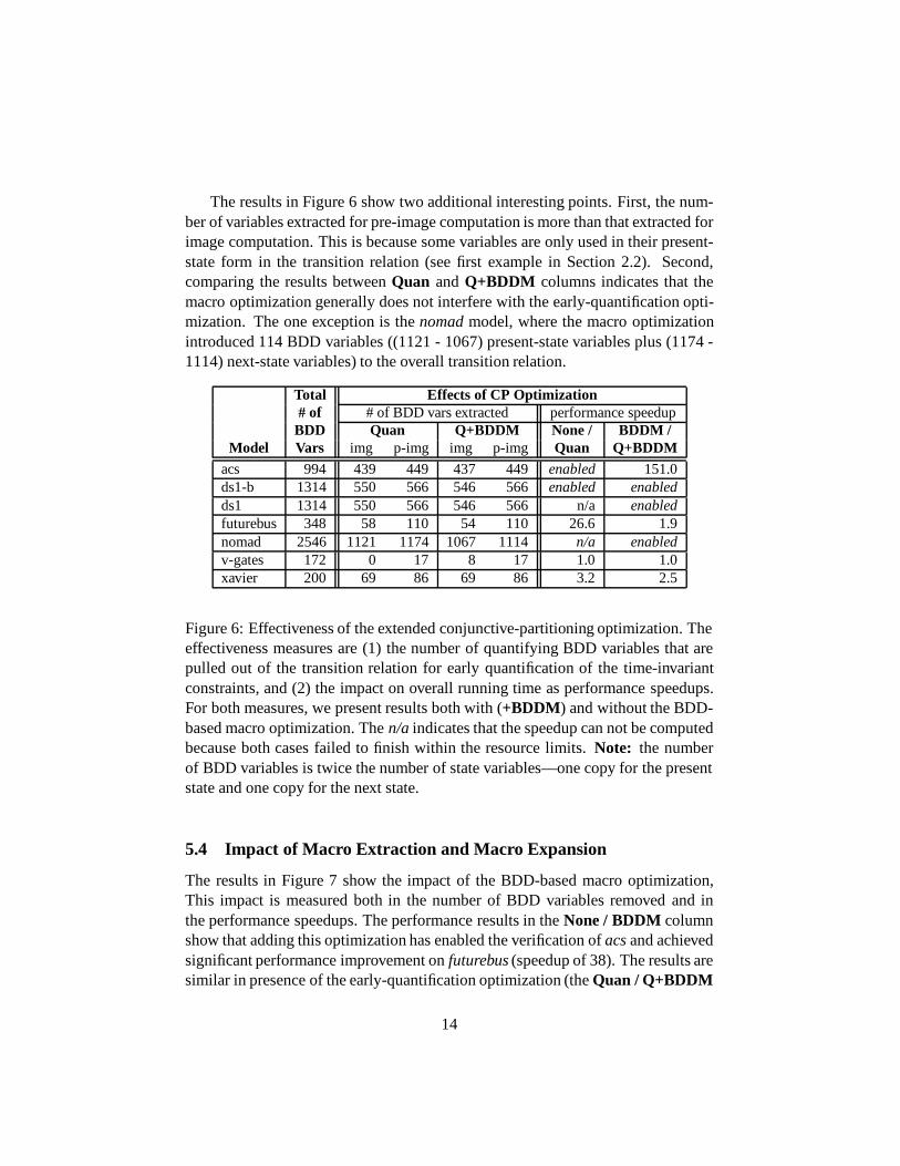
The results in Figure 6 show two additional interesting points. First, the num-ber of variables extracted for pre-image computation is more than that extracted forimage computation. This is because some variables are only used in their present-state form in the transition relation (see first example in Section 2.2). Second,comparing the results betweenQuan andQ+BDDM columns indicates that themacro optimization generally does not interfere with the early-quantification opti-mization. The one exception is thenomadmodel, where the macro optimizationintroduced 114 BDD variables ((1121 - 1067) present-state variables plus (1174 -1114) next-state variables) to the overall transition relation.

Total Effects of CP Optimization# of # of BDD vars extracted performance speedupBDD Quan Q+BDDM None / BDDM /

Model Vars img p-img img p-img Quan Q+BDDMacs 994 439 449 437 449 enabled 151.0ds1-b 1314 550 566 546 566 enabled enabledds1 1314 550 566 546 566 n/a enabledfuturebus 348 58 110 54 110 26.6 1.9nomad 2546 1121 1174 1067 1114 n/a enabledv-gates 172 0 17 8 17 1.0 1.0xavier 200 69 86 69 86 3.2 2.5

Figure 6: Effectiveness of the extended conjunctive-partitioning optimization. Theeffectiveness measures are (1) the number of quantifying BDD variables that arepulled out of the transition relation for early quantification of the time-invariantconstraints, and (2) the impact on overall running time as performance speedups.For both measures, we present results both with (+BDDM) and without the BDD-based macro optimization. Then/a indicates that the speedup can not be computedbecause both cases failed to finish within the resource limits.Note: the numberof BDD variables is twice the number of state variables—one copy for the presentstate and one copy for the next state.

5.4 Impact of Macro Extraction and Macro Expansion

The results in Figure 7 show the impact of the BDD-based macro optimization,This impact is measured both in the number of BDD variables removed and inthe performance speedups. The performance results in theNone / BDDM columnshow that adding this optimization has enabled the verification ofacsand achievedsignificant performance improvement onfuturebus(speedup of 38). The results aresimilar in presence of the early-quantification optimization (theQuan / Q+BDDM

14

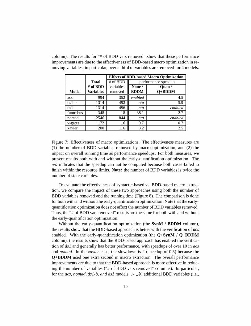
column). The results for “# of BDD vars removed” show that these performanceimprovements are due to the effectiveness of BDD-based macro optimization in re-moving variables; in particular, over a third of variables are removed for 4 models.

Effects of BDD-based Macro OptimizationTotal # of BDD performance speedup

# of BDD variables None / Quan /Model Variables removed BDDM Q+BDDM

acs 994 352 enabled 4.5ds1-b 1314 492 n/a 5.9ds1 1314 496 n/a enabledfuturebus 348 18 38.1 2.7nomad 2546 844 n/a enabledv-gates 172 16 0.7 0.7xavier 200 116 3.2 2.5

Figure 7: Effectiveness of macro optimizations. The effectiveness measures are(1) the number of BDD variables removed by macro optimization, and (2) theimpact on overall running time as performance speedups. For both measures, wepresent results both with and without the early-quantification optimization. Then/a indicates that the speedup can not be computed because both cases failed tofinish within the resource limits.Note: the number of BDD variables is twice thenumber of state variables.

To evaluate the effectiveness of syntactic-based vs. BDD-based macro extrac-tion, we compare the impact of these two approaches using both the number ofBDD variables removed and the running time (Figure 8). The comparison is donefor both with and without the early-quantification optimization. Note that the early-quantification optimization does not affect the number of BDD variables removed.Thus, the “# of BDD vars removed” results are the same for both with and withoutthe early-quantification optimization.

Without the early-quantification optimization (theSynM / BDDM column),the results show that the BDD-based approach is better with the verification ofacsenabled. With the early-quantification optimization (theQ+SynM / Q+BDDMcolumn), the results show that the BDD-based approach has enabled the verifica-tion of ds1and generally has better performance, with speedups of over 10 inacsandnomad. In thexavier case, the slowdown is 2 (speedup of 0.5) because theQ+BDDM used one extra second in macro extraction. The overall performanceimprovements are due to that the BDD-based approach is more effective in reduc-ing the number of variables (“# of BDD vars removed” columns). In particular,for theacs, nomad, ds1-b, and ds1models,> 150 additional BDD variables (i.e.,

15

> 75 state bits) are removed in comparison to using syntactic analysis.

Total Syntax vs. BDD-based Macro Optimization# of # of BDD vars removed performance speedupBDD SynM or BDDM or SynM / Q+SynM /

Model Vars Q+SynM Q+BDDM BDDM Q+BDDMacs 994 82 352 enabled 10.8ds1-b 1314 148 492 n/a 2.5ds1 1314 220 496 n/a enabledfuturebus 348 12 18 2.1 1.8nomad 2546 688 844 n/a 12.3v-gates 172 16 16 1.0 1.0xavier 200 64 116 1.2 1 / 2 = 0.5

Figure 8: Syntactic-based vs. BDD-based macro optimization. The effectivenessmeasures are (1) the number of BDD variables removed, and (2) the impact onoverall running time as performance speedups. For both measures, we present re-sults both with and without the early-quantification optimization. Then/a indicatesthat the speedup can not be computed because both cases failed to finish within theresource limits.Note: the number of BDD variables is twice the number of statevariables.

5.5 Impact of Conjunctive-Partitioning Size Limit

Because the conjunctive-partitioning algorithm often produces significantly dif-ferent performance results with different partition-size limits, we have also re-evaluated the above results using a partition-size limit of 100,000 nodes. The newresults generally follow the same trend as before with the exception ofds1-bandds1. For these two models, the results (Figure 9) show that if we choose the rightpartition-size limit foreach case, we do not need to perform the macro optimiza-tion to verify them. (Note that this is not always true; e.g., thenomadmodel cannotbe verified without the macro optimization.) However, with the BDD-based macrooptimization (theQ+BDDM column), the performance results are more stable andare generally much better.

6 Related Work

There have been many research efforts on BDD-based redundant state-variableremoval in both logic synthesis and verification. These research efforts all use

16

PartitionSize Limit None Quan SynM BDDM Q+SynM Q+BDDM

Model (# of nodes) (sec) (sec) (sec) (sec) (sec) (sec)

ds1-b 10,000 m.o. 321 t.o. m.o. 138 54ds1-b 100,000 t.o. 309 t.o. m.o. t.o. 101ds1 10,000 m.o. m.o. m.o. t.o. t.o. 37ds1 100,000 m.o. 255 t.o. m.o. 92 74

Figure 9: Effects of the partition-size limit. Them.o.’s andt.o.’s are the results thatexceeded the 900-MB memory limit and the 6-hour time limit, respectively.

the reachable state space (set of states reachable from initial states) to determinefunctional dependencies for Boolean variables (macro extraction). The reachablestate space effectively plays the same role as a time-invariant constraint, becausethe verification process only needs to check specifications in the reachable statespace.

Berthet et al. propose the first redundant state-variable removal algorithm in[3]. In [10], Lin and Newton describe a branch-and-bound algorithm to identifythe maximum set of redundant state variables. In[13], Sentovich et al. proposenew algorithms for latch removal and latch replacement in logic synthesis. Thereis also some work on detecting and removing redundant state variables while thereachable state space is being computed[9, 15].

From the algorithmic point of view, our approach is different from prior workin two ways. First, in determining the relationship between variables, the algo-rithms used to extract functional dependencies in previous work can be viewedas direct extraction of deterministic assignments to Boolean variables. In compari-son, our assignment extraction algorithm is more general because it can also handlenon-Boolean variables and extract non-deterministic assignments. Second, in per-forming the redundant state-variable removal, the approach used in the previouswork would need to combine all the constraints first and then extract the macrosdirectly from the combined result. However, for constraint-rich models, it may notbe possible to combine all the constraints because the resulting BDD is too largeto build. Our approach addresses this issue by first applying the assignment ex-traction algorithm to each constraint separately and then combining the results todetermine if a macro can be extracted (see Figure 1).

Another difference is that in previous work, the goal is to remove as manyvariables as possible. However, we have empirically observed that in some cases,removing additional variables can result in significant performance degradation inoverall verification time (slowdown over 4). To address this issue, we use simple

17

heuristics (size of the macro and the growth in graph sizes) to choose the set ofmacros to expand. This simple heuristic works well in the test cases we tried.However, in order to fully evaluate the impact of different heuristics, we need togather a larger set of constraint-rich models from a wider range of applications.

7 Conclusions and Future Work

The two optimizationswe proposed are crucial in verifying this new class of constraint-rich applications. In particular, they have enabled the verification of real-worldapplications such as the Nomad robot and the NASA Deep Space One spacecraft.

We have shown that the BDD-based assignment-extraction algorithm is effec-tive in identifying macros. We plan to use this algorithm to perform a more precisecone-of-influence analysis with the assignment expressions providing the exact de-pendence information between the variables. In general, we plan to study howBDDs can be use to further help other compile-time optimizations in symbolicmodel checking.

Acknowledgement

We thank Ken McMillan for discussions on the effects of macro expansion. Wethank Olivier Coudert, Fabio Somenzi and reviewers for comments on this work.We are grateful to Intel Corporation for donating the machines used in this work.

A Correctness Proof for Assignment-Extraction Algorithm

In this section, we present a correctness proof for the assignment-extraction algo-rithm in Section 4.1. Before presenting the main result, we first state and prove twosupporting lemmas.

Lemma 1 Let care-opt be any care-space optimization. Then, for arbitrary setexpressiont, Boolean formulah, and variablev,

(v 2 care-opt(t; h))^ h = care-opt(v 2 t; h) ^ h:

ProofBy the definition of the care-space optimization, we have the following prop-erties:

h ) (care-opt(t; h) == t);

h ) [care-opt(v 2 t; h) == (v 2 t)]:

18

Therefore,

(v 2 care-opt(t; h))^ h = (v 2 t) ^ h

= care-opt(v 2 t; h)^ h:

2

Lemma 2 Given an arbitrary Boolean formulaf and a variablev. Let

t =[

k2Kv

ITE(f jv k ; fkg; ;);

whereKv is the set of all possible values of variablev. Then,

(v 2 t) = f:

Proof

v 2 t =_

k02Kv

(v == k0) ^ (k0 2 t)

=_

k02Kv

(v == k0) ^ [k0 2[

k2Kv

ITE(f jv k; fkg; ;)]

=_

k02Kv

(v == k0) ^_

k2Kv

[k0 2 ITE(f jv k ; fkg; ;)]

=_

k02Kv

(v == k0) ^_

k2Kv

ITE(f jv k; k0 2 fkg; k0 2 ;)

=_

k02Kv

(v == k0) ^_

k2Kv

ITE(f jv k; k0 2 fkg; 0)

=_

k02Kv

(v == k0) ^ ITE(f jv k0 ; k0 2 fk0g; 0)

=_

k02Kv

(v == k0) ^ ITE(f jv k0 ; 1; 0)

=_

k02Kv

(v == k0) ^ f jv k0

= f:

2

Using the two lemmas above, we can now prove the correctness of the assignment-extraction algorithm.

19

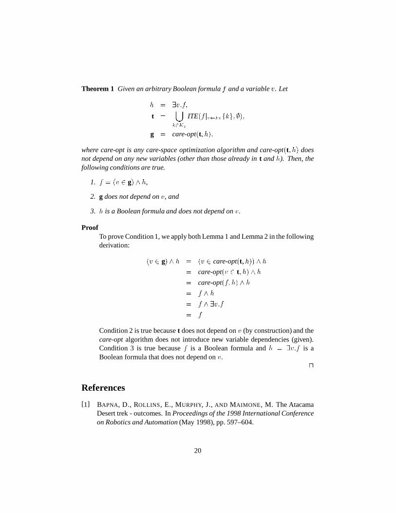
Theorem 1 Given an arbitrary Boolean formulaf and a variablev. Let

h = 9v:f;

t =[

k2Kv

ITE(f jv k; fkg; ;);

g = care-opt(t; h);

where care-opt is any care-space optimization algorithm and care-opt(t; h) doesnot depend on any new variables (other than those already int andh). Then, thefollowing conditions are true.

1. f = (v 2 g) ^ h,

2. g does not depend onv, and

3. h is a Boolean formula and does not depend onv.

ProofTo prove Condition1, we apply both Lemma 1 and Lemma 2 in the followingderivation:

(v 2 g) ^ h = (v 2 care-opt(t; h))^ h

= care-opt(v 2 t; h) ^ h

= care-opt(f; h) ^ h

= f ^ h

= f ^ 9v:f

= f

Condition 2 is true becauset does not depend onv (by construction) and thecare-optalgorithm does not introduce new variable dependencies (given).Condition 3 is true becausef is a Boolean formula andh = 9v:f is aBoolean formula that does not depend onv.

2

References

[1] BAPNA, D., ROLLINS, E., MURPHY, J.,AND MAIMONE, M. The AtacamaDesert trek - outcomes. InProceedings of the 1998 International Conferenceon Robotics and Automation(May 1998), pp. 597–604.

20

[2] BERNARD, D. E., DORAIS, G. A., FRY, C., JR., E. B. G., KANEFSKY, B.,KURIEN, J., MILLAR , W., MUSCETTOLA, N., NAYAK , P. P., PELL, B.,RAJAN, K., ROUQUETT, N., SMITH , B., AND WILLIAMS , B. Design ofthe remote agent experiment for spacecraft autonomy. InProceedings of the1998 IEEE Aerospace Conference(March 1998), pp. 259–281.

[3] BERTHET, C., COUDERT, O., AND MADRE, J. C. New ideas on symbolicmanipulations of finite state machines. In1990 IEEE Proceedings of theInternational Conference on Computer Design(September 1990), pp. 224–227.

[4] BRYANT, R. E. Graph-based algorithms for Boolean function manipulation.IEEE Transactions on Computers C-35, 8 (August 1986), 677–691.

[5] BURCH, J. R., CLARKE, E. M., LONG, D. E., MCMILLAN , K. L., AND

DILL , D. L. Symbolic model checking for sequential circuit verification.IEEE Transactions on Computer-Aided Design of Integrated Circuits andSystems 13, 4 (April 1994), 401–424.

[6] CLARKE, E. M., MCMILLAN , K. L., ZHAO, X., FUJITA, M., AND YANG,J. C.-Y. Spectral transform for large Boolean functions with application totechnology mapping. InProceedings of the 30th ACM/IEEE Design Automa-tion Conference(June 1993), pp. 54–60.

[7] COUDERT, O., AND MADRE, J. C. A unified framework for the formalverification of circuits. InProceedings of the International Conference onComputer-Aided Design(Feb 1990), pp. 126–129.

[8] GEIST, D., AND BEER, I. Efficient model checking by automated order-ing of transition relation partitions. InProceedings of the Computer AidedVerification(June 1994), pp. 299–310.

[9] HU, A. J., AND DILL , D. L. Reducing BDD size by exploiting functionaldependencies. InProceedings of the 30th ACM/IEEE Design AutomationConference(June 1993), pp. 266–71.

[10] LIN, B., AND NEWTON, A. R. Exact redundant state registers removal basedon binary decision diagrams.IFIP Transactions A, Computer Science andTechnology A, 1 (August 1991), 277–86.

[11] MCMILLAN , K. L. Symbolic Model Checking. Kluwer Academic Publish-ers, 1993.

21

[12] RANJAN, R. K., AZIZ, A., BRAYTON, R. K., PLESSIER, B., AND PIXLEY,C. Efficient BDD algorithms for FSM synthesis and verification. Presentedin the IEEE/ACM International Workshop on Logic Synthesis, May 1995.

[13] SENTOVICH, E. M., AND HORIA TOMA, G. B. Latch optimization in cir-cuits generated from high-level descriptions. InProceedings of the Interna-tional Conference on Computer-Aided Design(November 1996), pp. 428–35.

[14] SHIPLE, T. R., HOJATI, R., SANGIOVANNI -VINCENTELLI, A. L., AND

BRAYTON, R. K. Heuristic minimization of BDDs using don’t cares. InPro-ceedings of the 31st ACM/IEEE Design Automation Conference(June 1994),pp. 225–231.

[15] VAN EIJK, C. A. J.,AND JESS, J. A. G. Exploiting functional dependenciesin finite state machine verification. InProceedings of European Design andTest Conference(March 1996), pp. 266–71.

[16] WILLIAMS , B. C., AND NAYAK , P. P. A model-based approach to reactiveself-configuring systems. InProceedings of the Thirteenth National Con-ference on Artificial Intelligence and the Eighth Innovative Applications ofArtificial Intelligence Conference(August 1996), pp. 971–978.

[17] YANG, B., BRYANT, R. E., O’HALLARON, D. R., BIERE, A., COUDERT,O., JANSSEN, G., RANJAN, R. K., AND SOMENZI, F. A performance studyof BDD-based model checking. InProceedings of the Formal Methods onComputer-Aided Design(November 1998), pp. 255–289.

22