optimizing prediction intervals by tuning random forest ... · meta-validation for tuning...

Noname manuscript No.(will be inserted by the editor)

Optimizing Prediction Intervals by Tuning RandomForest via Meta-Validation

Sean Bayley · Davide Falessi

the date of receipt and acceptance should be inserted later

Abstract Recent studies have shown that tuning prediction models increases pre-diction accuracy and that Random Forest can be used to construct prediction in-tervals. However, to our best knowledge, no study has investigated the need to,and the manner in which one can, tune Random Forest for optimizing predictionintervals – this paper aims to fill this gap. We explore a tuning approach thatcombines an effectively exhaustive search with a validation technique on a singleRandom Forest parameter. This paper investigates which, out of eight validationtechniques, are beneficial for tuning, i.e., which automatically choose a RandomForest configuration constructing prediction intervals that are reliable and with asmaller width than the default configuration. Additionally, we present and vali-date three meta-validation techniques to determine which are beneficial, i.e., thosewhich automatically chose a beneficial validation technique. This study uses datafrom our industrial partner (Keymind Inc.) and the Tukutuku Research Project,related to post-release defect prediction and Web application effort estimation,respectively. Results from our study indicate that: i) the default configuration isfrequently unreliable, ii) most of the validation techniques, including previouslysuccessfully adopted ones such as 50/50 holdout and bootstrap, are counterpro-ductive in most of the cases, and iii) the 75/25 holdout meta-validation techniqueis always beneficial; i.e., it avoids the likely counterproductive effects of validationtechniques.

Keywords Tuning · validation · prediction intervals · confidence intervals ·defect prediction · effort estimation.

Sean BayleyDept. of Computer Science and Engineering, Notre DameE-mail: [email protected]

Davide FalessiDept. of Computer Science and Software Engineering, California Polytechnic State UniversityE-mail: [email protected]

arX

iv:1

801.

0719

4v1

[cs

.LG

] 2

2 Ja

n 20

18

2 Sean Bayley, Davide Falessi

1 Introduction

One important phase of software development is release planning [77]. Duringrelease planning, stakeholders define characteristics of the software release suchas the requirements to implement, the defects to fix, the developers to use, theamount and type of testing, and the release duration. The project manager mustmake decisions in the midst of conflicting goals like time-to-market, cost, number ofexpected defects, and customer demands. These business goals, their importance,and clients’ expectations vary among releases of the same or different projects, andin turn the number of acceptable defects varies. For instance, some projects aremore safety critical than others and, therefore, can tolerate fewer defects. Thus,the manager might decide to increase the amount of testing, reduce the number offeatures, or postpone the release deadline if the predicted number of defects doesnot fit the business goals of that project release.

In 2011, Keymind developed and institutionalized a tool to help managersdefine characteristics of a software release according to the predicted number ofpost-release defects. Over the last seven years, the tool was subject to eight majorupgrades. Each upgrade included refreshing the data (i.e., collecting data aboutnew software releases), refreshing the type of data (i.e., adding metrics based onchanges in technologies being used), improving the usability of the layout, andselecting the most accurate prediction models. A major improvement effort tookplace in 2013, when Keymind transitioned from predicting the number of defectsto predicting the upper bounds related to a confidence level [31]. Thus, Keymindmoved from supporting a sentence such as “The expected number of defects isy” to supporting a sentence such as “We are 90% confident that the numberof defects is less than y.” Then, during a discussion with the Keymind team in2016, we learned that the current model was actionable but not fully explicative.Specifically, we realized that an interval is more informative than its upper-bound,i.e., the lower bound is also informative. For instance, there is a practical differencein the intervals 0 ≤ y ≤ 10 and 9 ≤ y ≤ 10 constructed for two different softwareprojects. On the one hand, the former is more desirable as the actual number ofpost-release defects could be 0, i.e., spending additional money on testing mightnot be required. On the other hand, the latter is more actionable, i.e., there is lessvariability. Upon reviewing the literature, we determined that prediction intervalscan be used to support the sentence “We are 90% confident that the number ofdefects is between a and b”, where a and b are the lower and upper bounds of theprediction interval [1, 40, 41].

1.1 Definitions

In order to avoid ambiguities in the remainder of this paper, we define the followingkey terms and concepts.

– Model: a formal description of structural patterns in data used to make pre-dictions (e.g., Random Forest) [94].

– Parameter: an internal variable of the algorithm used to learn the model (e.g.,MTRY [94]).

– Configuration: the set of values for each of the parameters of a model (e.g.,MTRY=1.0 and all other parameters set as default).

Optimizing Prediction Intervals by Tuning Random Forest via Meta-Validation 3

Model evaluation

Validation for tuning

Meta-validation for tuning Train'' Test'' Unused

Train' Test'

Train Test

Unused

Time

Fig. 1: Data used for model evaluation, validation and meta-validation for tuning.

– Prediction Interval (PI): an estimate of an interval, with a certain proba-bility, in which future observations will fall (e.g., 0 ≤ post-release defects ≤ 5)[34]. An important difference between the confidence interval (CI) and the PIis that the PI refers to the uncertainty of an estimate, while the CI refers tothe uncertainty associated with the parameters of a distribution [41], e.g., theuncertainty of the mean value of a distribution of values.

– Width: the size of a PI. Width is computed as the upper bound minus thelower bound, e.g., Width(0 ≤ y ≤ 5) = 5. The smaller the width, the better.

– Coverage: also called coverage probability, hit-rate, or actual confidence, isthe proportion of time the true value falls within the PI [25]. For instance, thetrue value might fall within the PI of a model 92% of the time. The higher thecoverage, the better.

– Nominal Confidence (NC): the stated proportion of time the true valueshould fall within the PI [25]. A project manager might like to have a modelthat constructs PI that contain the true value 90% of the times, i.e., the nominalconfidence is 90%.

– Reliable: refers to a model that constructs PIs such that Coverage ≥ NC.For instance, a model is said to be reliable if nominal confidence is 90% andcoverage is 92%. Reliable models are preferable.

– Best Configuration: with respect to PI, the goodness of a configuration is (1)contingent upon reliability and (2) inversely proportional to width. Thus, wedefine the best configuration as the configuration with smallest width amongthe set of reliable configurations.

– Model evaluation: the process of measuring the performance of a model, asconfigured in a specific way (i.e., default configuration). Typically the modelis first trained (i.e., learned) and then it is tested (i.e., accuracy is measured).For instance, in Figure 1, the dataset is first ordered chronologically and thensplit in two parts: train and test. Note that the proportion of train and test(i.e., 66/33) is consistent in Fu et al. [33] and Tantithamthavorn et al. [85].We also note that there are validation techniques that split the dataset inproportions other than 66/33 or that do not even preserve the order of thedata between training and testing. We discuss validation techniques in furtherdetail in Section 2.6.

– Tuning, auto-configuration, or configurations validation: is the processof automatically finding the model configuration which optimizes an objectivefunction [6, 89]. In our context, we are interested in selecting the configura-tion which constructs the narrowest reliable PI. In this work, because we letonly one parameter vary, and because we evaluate all possible values of saidparameter, a tuning technique coincides with an exhaustive search and a spe-cific validation technique. Thus, in this work, the terms tuning technique andvalidation technique can be used interchangeably. Tuning uses the training set


of the model evaluation for validating candidate model configurations. Specif-ically, in Figure 1, the evaluation training set is divided into train′ and test′ oftuning. We note that train and test sets of tuning can be of different propor-tions; the only constraint of a tuning technique is that it is not exposed to theevaluation test set.

– Beneficial: refers to a tuning technique that is able to select a configura-tion that constructs PIs that are reliable and narrower than what the defaultconfiguration constructs.

– Configuration meta-validation: aka meta-validation, is the process of auto-matically finding the most beneficial tuning technique. In other words, if tuningselects the best configuration, by validating the different configurations, meta-validation selects the best technique to select the best configuration. Meta-validation uses the tuning training set for validating the tuning techniques.In Figure 1, the train′ subset is further divided into train′′ and test′′. Again,training and test sets can have different proportions; the only constraint is thatno meta-validation subset use test or test′.

1.2 Motivation

In order to better understand the problem we are trying to solve, Figure 2 reportsPIs at NC90 (green), NC95 (blue), and NC99 (yellow) as constructed by the defaultrandom forest configuration on the Keymind dataset. The model is trained on thefirst 66% of the data and PIs are constructed for the remaining 33%. We plotthe actual number of post-release defects with the same color of the narrowestinterval in which it is contained, e.g., a green point indicates that the actual valueis contained in the PI constructed at NC90. We plot points that are not containedat any NC as red. Lastly, we plot the predicted value with a “x”.

In Figure 2, we observe that NC90 covers 89% (106), NC95 covers 95% (113),and NC99 covers 98% (117) of the total (119) releases. In other words, the defaultrandom forest configuration is not reliable at NC90 and NC99. Thus, we cannotuse the default configuration to support the claim “We are NC % confident thatthe number of defects is between a and b” if NC is 90 or 99. This motivates theneed for tuning to choose a configuration, other than default, which constructsreliable PIs.

Figure 2 is also useful to identify the differences between PIs and CIs. Specifi-cally, there are cases in which the NC95 and NC99 intervals cannot be seen (e.g.,release 252). This means that the intervals constructed at all NCs are equivalent.This denotes a significant difference between PIs and CIs: the width of CIs isstrongly correlated with NC. Moreover, within the same NC, higher upper boundsdo not always correspond with more predicted defects. For example, release 280has a higher number of predicted defects than release 267 but a lower upper boundat NC95 and NC99. This denotes another significant difference between PIs andCIs. Specifically, within the same NC, the upper bound of CIs is strongly correlatedwith the predicted number (i.e., NC50).

Finally, it is interesting to note that larger intervals do not always correspondwith more actual defects. For example, release 248 has the second most defects andthe 27th, 33rd, and 47th largest interval for NC90, NC95, and NC99, respectively.


245 256 267 278 289 300 311 322 333 344 355 363

Release ID

Post

-rele

ase

defe

cts

Fig. 2: Prediction intervals at NC90 (green), NC95 (blue), and NC99 (yellow) asconstructed by the default random forests configuration on the Keymind dataset.The model is trained on the first 66% of the data and PIs are constructed for theremaining 33%.

1.3 Aim

Recent studies have shown that tuning prediction models increases accuracy [10,22, 23, 26, 33], and that Random Forest can be used to to predict defect and effortdata [66, 80] and to construct prediction intervals. However, to our best knowledge,no study has investigated the need, or how, to tune Random Forest for optimizingprediction intervals; this paper aims to fill this gap.

The contribution of this paper is threefold;

1. We use Random Forest to construct prediction intervals for software engineer-ing data (fault and effort).

2. We present and evaluate the use of eight validation techniques for tuning todetermine which are beneficial.

3. We present and evaluate three meta-validation techniques to determine whichare beneficial, i.e., which automatically choose a beneficial validation technique.

Specifically, we investigate the following research questions.

RQ 1 Is default the best configuration?

RQ 2 Are validation techniques beneficial?

RQ 3 Are meta-validation techniques beneficial?

Our validation uses data from our industrial partner (Keymind Inc.) and theTukutuku Research Project, containing 363 and 195 industrial data points related


to post-release defect prediction and Web application effort estimation, respec-tively.

Results show that the default configuration is frequently unreliable and previ-ously successfully adopted validation techniques, such as 50/50 holdout and boot-strap, are frequently counterproductive in tuning. Moreover, no single validationtechnique is always beneficial; however, the meta 75/25 holdout technique selectsvalidation techniques that are always beneficial. Thus, results show that RandomForest is a viable solution to construct prediction intervals only if well tuned. Be-cause no single validation technique resulted always beneficial, we recommend theuse of meta 75/25 holdout meta-validation technique to dynamically chose thevalidation technique according to the dataset and prediction interval of interest.

In order to support the usability and replicability of this study, we provide aPython package for tuning and meta-tuning Random Forests PIs. We also showhow to use it over a large open source project called Apache-ANT.

1.4 Structure

The remainder of the paper is structured as follows. Section 2 discusses relatedwork. Section 3 describes our experimental design. Section 4 present results anddiscussion. Section 5 presents meta tune, an open source Python package we de-veloped for using and tuning prediction intervals. Section 6 discusses threats tovalidity. Section 7 concludes the paper and identifies areas for future work.

2 Related Work

2.1 Defect Prediction

Numerous recent studies have applied data mining and machine learning tech-niques to improve QA resource allocation, i.e., to focus QA efforts on artifact(s)expected to be the most defective. These studies can be generally categorized asdefect classification (i.e., the artifact is either defective or not defective) [2, 35–37, 45, 46, 60–64, 70, 71, 76, 81, 84, 91, 96, 97] or defect prediction (i.e., the artifactcontains n defects) [7, 8, 54, 72, 87, 88].

Similar to this paper, Li et al. [54] investigate the use of post-release defectprediction in the planning of widely used multi-release commercial systems. Theyconclude that models currently available fall short because they do not adequatelyconsider organizational changes and customer adoption characteristics.

A family of studies apply capture-recapture to defect prediction [8, 71, 72,87, 88]. These studies estimate the remaining number of defects by analyzingcharacteristics of the overlapping set of defects detected by multiple, independentreviewers. Capture-recapture was first applied to software inspections by Eick et al.[28] in 1992 and Petersson et al. [72] provide a survey of the method.

2.2 Effort Prediction

It is often difficult to predict the amount of effort required to complete a softwareproject due to changes associated with aspects of software development (e.g., re-


quirements, development environments, and personnel). It is of practical impor-tance to have accurate effort predictions as it affects project management andresource allocation, i.e., larger parts of the budget should be allocated for artifactsthat are expected to require more effort. Software effort prediction has been thesubject of numerous studies, as summarized by Boehm et al. [9] and Molokkenand Jorgensen [67].

Jørgensen and Moløkken [40] use independent expert opinions to predict theamount of development effort. They suggest that it is better to have estimationteams comprising several different types of roles, rather than estimation teamsconsisting of only technical roles, to help reduce systematic bias. We incorporatethis suggestion into the development of the Keymind dataset, which we discussfurther in Section 3.1.1.

Briand et al. [17] develop and apply CoBRA, a hybrid method which com-bines aspects of algorithmic and experiential approaches, to predicting the cost ofsoftware development. To construct CoBRA, domain experts are asked to decidethe causal factors and their possible values. Experimental results show realisticuncertainty estimates. However, this method requires, and is sensitive to, humanestimates.

Di Martino et al. [23] propose and validate the use of a Genetic Algorithmwith a grid search for tuning support vector regression for estimating defectivefile. Corazza et al. [22] propose and validate a meta-heuristics Tabu Search fortuning support vector regression for point values effort estimation. Their resultsshow that Tabu search outperformed other simpler approaches, such as randomconfiguration and default configuration. Because in this work it is reasonable totune only one parameter, then a full search is preferable to any other incompletesearch such as the Genetic or Tabu types.

Whigham et al. [93] propose a baseline for comparing effort estimation models.Unfortunately such a baseline does not apply to prediction interval and thereforecannot be used in this work.

To the best of our knowledge, there has been no study that has applied RandomForest to effort prediction.

2.3 Intervals in Software Engineering

Predictions about the number of post-release defects or development effort areintrinsically uncertain. This uncertainty primarily arises as a result of the natureof software development (e.g., changing requirements, unstable development teamsand environments). However, there is also some degree of uncertainty associatedwith the model used to make the prediction. Hence, information about the levelof uncertainty is desirable.

Software engineering studies using intervals can be generally categorized aseither using CIs in combination with capture-recapture methods [71, 72, 87, 88],or constructing PIs from expert opinion elicitation [40], bootstrapping [1], regres-sion models [12], a combination of cluster analysis and classification methods [3],amulti-objective evolutionary algorithm [79], or based on prior estimates [41]. Wenote that linear regression is not typically used in the construction of predic-tion intervals with respect to software engineering predictions. In our case, our


datasets violated multiple assumptions of linear regression such as normality andhomoscedasticity; thus, we did not consider it as a viable approach.

Thelin and Runeson [88] show that model-based point estimates, when usedwith confidence intervals, outperform human-based estimates. This result is par-ticularly relevant as previous studies conclude that human-based estimates out-perform model-based point estimates.

Vander Wiel and Votta [92] evaluate Walds Likelihood CI and MhJK CIs andconclude that the Walds Likelihood CI includes the correct number of defects inmost cases, and therefore should be preferred over Mh-JK. However, the WaldsLikelihood CI is often too conservative, which leads to large intervals [72].

Notably, Angelis and Stamelos [1] describe an instance-based learning approachused in combination with bootstrapping to construct effort intervals. They claim toconstruct CIs, however, our reading of the paper suggests they actually constructPIs.

Jørgensen and Sjoeberg [41] introduce an approach used to construct effort PIbased on the assumption that they are able to select prior projects with similarestimation errors to that of a future project, i.e., the selected projects must havesimilar degrees of uncertainty as the future project.

Regarding PI construction via expert-opinion elicitation, Jørgensen and Moløkken[40] use human-based PIs in effort estimation and conclude that group-discussionbased PIs are more effective than mechanically combining individual PIs. However,the approach they put forth requires significant time and effort on the part of theexperts involved and is sensitive to the accuracy of human estimates. Further, PIsbased on human estimates tend to be too narrow to reflect high confidence levels(e.g., 90% nominal confidence) [21, 42].

In conclusion, despite significant research advances in predictive models forsoftware analytics, there have been very few studies that investigate the use ofmodel-based intervals (CI or PI). A majority of those that have rely on capture-recapture methods [8, 71, 72, 87, 88], which are a very specific type of predictionand have the distinct disadvantage of requiring human review. Methods relyingon human estimates [17, 40, 88] are infeasible in our context. To our knowledge,no SE studies have investigated constructing PIs with Random Forest.

2.4 Random Forest

Decision trees are attractive for their execution time and the ease with which theycan be interpreted. However, decision trees tend to overfit and generalize poorlyto unseen data [94]. The Random Forest (RF), first introduced in 1995 by TinKam Ho [38], is an example of ensemble learning in which multiple decision treesare grown independently.

Given data-points Di and responses yi, i = 1, . . . ,m, each decision tree is grownfrom a bootstrapped sample of D. Further, only a random subset of predictors isconsidered for the split of each node [14]. The number of predictors to consider ateach split is specified by the parameter MTRY.

Thus, the trees grown in different, random subspaces generalize in a comple-mentary manner, and their combined decision can be monotonically improved[14, 38]. Given data-points Di and responses yi, i = 1, . . . ,m, where each Dicontains n predictors, each tree in the RF is grown as follows:


Fig. 3: Random Forest overview.

– Construct the training set by sampling, with replacement, m data-points fromD.

– At each node, n′ = n×MTRY predictors are selected randomly and the mostinformative of these n′ predictors is used to split the node.

– Each tree is grown to the largest extent possible.

The prediction y of a single tree T for a new data-point X = x is obtainedby averaging the observed values `(x), where ` is the leaf that is reached whendropping x down T .

The prediction of a Random Forest y is equivalent to the conditional meanµ(x) which is approximated by averaging the prediction of the k trees [14]:

y = µ(x) = k−1k∑i=1

`k(x). (1)

Guo et al. [36] were the first to investigate the use of RF in defect classification.They conclude that RF outperforms the logistic regression and discriminant anal-ysis of SAS1, the VF1 and VotedPerceptron classifiers of WEKA2, and NASA’sROCKY [59].

2.5 Random Forest Prediction Intervals

A common goal in statistical analysis is to infer the relationship between a responsevariable, Y ∈ R, and a predictor variable X. Given X = x, typical regressionanalysis determines an estimate µ(x) of the conditional mean of Y . However, theconditional mean describes just one aspect of the relationship, neglecting otherfeatures such as fluctuations around the predicted mean [56]. In general, givenX = x the distribution function is defined by the probability that Y ≤ y [29]:

F (y|x) = P (Y ≤ y|X = x). (2)

1 http://www.sas.com2 http://www.cs.waikato.ac.nz/ml/weka/


For a continuous distribution, the τ -quantile is defined such that τ = F (y|X = x)[56]:

Qτ (x) = inf{y : F (y|X = x) ≥ τ}. (3)

We can use these definitions to construct PIs. For instance, the 90% predictioninterval is given by:

I.90(x) = [Q.05(X = x), Q.95(X = x)] (4)

In other words, there is a 90% probability that a new observation of Y is containedin the interval. Meinshausen [56] presents the Quantile Regression Forest (QRF),a general method for constructing prediction intervals based on decision trees.Rather than approximating the conditional mean, he shows that the responsesfrom each tree Ti, i = 1, . . . , k can be used to approximate the full conditionaldistribution function F (y|X = x).

We can use the RF to construct prediction intervals if we ensure that all treesare fully expanded, i.e., each leaf has only one response. For a given X = x andRF with trees Ti, i = 1, . . . , k, the distribution function can be approximated as:

F (y|x) = k−1k∑i=1

1{`i(x)≤y}. (5)

In other words, the likelihood that the prediction yi = `i(x) is less than or equalto the response y. Then, the τ -quantile can be approximated as:

Qτ (x) = inf{y : F (y|X = x) ≥ τ}. (6)

Finally, the 90% prediction interval can be approximated as:

I.90(x) = [Q.05(X = x), Q.95(X = x)]. (7)

We note that it is possible that we are unable to fully expand all of the trees. Thiscan happen if (1) the node is already pure, or (2) the node cannot be split further,i.e., all remaining data-points have the same predictors. In the former case, weknow the response and the leaf size, i.e., we can still determine the conditionaldistribution. In the latter case, we do not know what the response would be if thenode is split further; hence, we are unable to determine the conditional distribu-tion. Lastly, we note that fully-expanding trees can lead to overfitting, in whichcase the intervals will provide little practical value [56]. However, fully expandingtrees is what Breiman [14] suggests. Further, even if individual trees overfit, theeffect should be mitigated by increasing the total number of trees in the forest.

We present the procedure for constructing prediction intervals in Algorithm 1.The procedure accepts four arguments: D (the data-points), y (the responses),nc (the nominal confidence), and ph (the percent to be held out). In lines 2-4 wepartition the data into training and test sets and learn a RF. In lines 7-11 werecord the responses of all decision trees for each di ∈ Dtest. We ensure that eachleaf is pure on line 10. Finally, we construct prediction intervals on line 17.

Table 1 presents the list of parameters for Sci-Kit Learn’s RandomForestRe-gressor.


Algorithm 1 Random Forest Prediction Intervals

1: procedure PredictionIntervals(D, y, nc, ph)2: D train,D test, y train, y test← split(D, y, ph)3: clf← RandomForestRegressor()4: clf.fit(D train, y train)5:6: preds← [[]]7: for all est in clf.estimators do8: for all n, leaf in est.apply(D test) do9: if leaf is not pure then

10: exit11: preds[n].extend(leaf.responses())

12:13: α← 1−nc

214: β ← 1− α15: intervals← []16: for all pred in preds do17: intervals.append((Qα(pred), Qβ(pred)))

18: return intervals19:20: procedure

Table 1: Sci-Kit Learn RandomForestRegressor parameters

feature description valuen estimators The number of trees in the for-

est.1000

max features The size of the subset of the fea-tures to consider for each split.

1.0*

max depth The maximum depth of the tree. Nonemin samples

splitThe minimum number of samples re-quired to split an internal node.

2

min samplesleaf

The minimum number of samples re-quired to be at a leaf node.

1

min weightfraction leaf

The minimum weighted fraction ofthe sum total of weights (of all the in-put samples) required to be at a leafnode.

0

max leaf nodes If specified, trees are grown with thespecified number of leaves in a bestfirst fashion.

None

min impuritysplit

Threshold for stopping early treegrowth.

1E-7

2.6 Validation Techniques

Validation techniques (also referred to as performance estimation techniques) aremethods used for estimating performance of a model on unseen data. They arewidely used in the machine learning domain to compare the performance of mul-tiple models on a dataset in order to select the most well suited model (i.e., themodel that minimizes the expected error) [27, 53, 68].

Within the context of validating defect prediction models, Tantithamthavornet al. [86] report 89 studies (49%) use k-fold cross-validation, 83 studies (45%) use


holdout validation, 10 studies (5%) use leave-one-out cross-validation, and 1 study(0.5%) uses bootstrap validation.

Validation techniques are also used in hyper-parameter optimization, i.e., tun-ing the parameters of a model [33, 85]. There are many validation techniquesthat can be applied and no consensus on which technique is the most effective[4, 13, 15, 47, 48, 65, 86].

To our knowledge, only two techniques have been used in tuning models forsoftware analytics: Fu et al. [33] use the holdout and Tantithamthavorn et al. [85]use bootstrap. These studies serve as inspiration for this work; we analyze the twotechniques used in their studies and include an additional six more. Moreover, wereuse part of their experimental design: we holdout one third of the initial datasetfor testing. One of the major differences in this paper is that both our datasets con-tain data-points measured across multiple industrial projects and multiple releasesof the same project, whereas each of their datasets contain data-points measuredfrom a single release of an open-source project. Thus, our datasets are sensitiveto time and this aspect could affect the performance of certain tuning techniquesthat do not preserve the dataset order (e.g., bootstrap) in learning and testing.

2.6.1 Order Preserving

Techniques which preserve the order of the dataset are commonly used for per-formance estimation with time-series data (e.g., forecasting) [5]. We analyze fivesuch techniques: time series cross-validation, time series HV cross-validation, andthree variations of the non-repeated holdout. Given data-points Di and responsesyi, i = 1, . . . ,m:

H/k holdout partitions the dataset such that hm data-points are used for training

and km are used for testing. Holdout validation has the advantage of being faster

than techniques which require multiple repetitions and is often acceptable to useif D is sufficiently large [94]. However, it is criticized for providing unreliableestimates [86] due to the fact that performance is estimated on a single subset ofD. Further, the holdout is criticized as being statistically inefficient since muchof the data is not used to train the model [86]. Figure 1 provides an example of66/33 holdout between validation-training and validation-testing.

Time series cross-validation (TSCV) computes an average of k-step aheadforecasts by the rolling-origin-calibration procedure [11]. Note that unlike standardcross-validation procedures, the i+ 1 training set is a super-set of all training sets[1, 2, . . . , i]. TSCV has the advantage of being relatively fast. However, theoreticalconcerns have been raised about dependencies between the data-points in thetraining and test sets [5].

Time series HV cross-validation [75] (TSHVCV) is an extension of the timeseries h-block cross validation introduced by Burman et al. [18] in 1994. TSHVCVremoves v data-points from both sides of Di, yielding a validation set of size2v + 1. Then, h data-points on either side of the validation set are removed. Theremaining n−2v−2h−1 data-points are used in training. The process is repeatedfor i ∈ [v + 0s, v + 1s, . . . ,m − v] where s is a specified step size. TSHVCV has


the benefit of being theoretically robust to data dependencies. However, it can becomputationally expensive if D is sufficiently large.

2.6.2 Non-Order Preserving

Techniques which do not preserve the order of the dataset are commonly usedin the general context of machine learning validation and are particularly effec-tive when data-points are not time sensitive. An example of non-sensitive datais the characteristics of classes and their defectiveness within a single softwarerelease of an open-source project. We analyze three such techniques: h × k-foldcross-validation, K out-of-sample bootstrapping, and leave-one-out cross-validation.Given data-points Di and responses yi, i = 1, . . . ,m:

K-fold cross-validation partitions the data into k equal sized folds: k − 1 foldsare used for training and the remaining fold is used for testing. This is repeateduntil each fold has been used for testing. H × k-fold cross-validation performsk-fold cross-validation h times, re-seeding the PRNG at each iteration. Cross-validation techniques have the advantage of utilizing all of the data-points in D fortraining. However, if D is time sensitive, cross-validation will construct trainingsets containing data-points measured after data-points in the test set. Further,cross-validation techniques have been shown to produce unreliable estimates if Dis small [13, 39].

K out-of-sample bootstrapping is a technique in which the dataset is randomlysampled with replacement. The training set is constructed by randomly samplingm data points with replacement from D. The out of bag samples are used fortesting. The bootstrap has the advantage of being more effective at providingaccurate estimates when D is small. However, the bootstrap can be misleadinglyoptimistic [94].

Leave-one-out cross-validation (LOO) is a case of k-fold cross-validation inwhich k = 1. LOOCV has the advantage of using the greatest possible amount ofdata-points in training at each iteration. Further, prior work in effort estimationhas shown that LOOCV is the least biased technique [47]. However, LOOCV hasalso been criticized for providing estimates with high variance [32].

2.7 Tuning

Recent software engineering studies indicate that configuring models can impactmodel performance [33, 50, 57, 85, 90].

Fu et al. [33] investigate whether tuning is necessary in software analytics.They find that tuning can increase model performance by 5-20%, and in one casethey show Precision can be improved from 0% to 60%. They report that 80% ofhighly-cited defect prediction studies use default model configurations and raiseconcerns about conclusions drawn from these studies regarding the superiority ofone model over another. They conclude that tuning is a necessary step beforeapplying a model to the task of defect prediction.

Tosun and Bener [90] investigate tuning with respect to defect classificationand found that using the default model configuration can produce sub-optimal


results. Specifically, they find that tuning the decision threshold of the Naive BayesClassifier can decrease false alarms by 34% to 24%.

Tantithamthavorn et al. [85] show that configuring models can increase per-formance by as much as 40% and increases the likelihood of producing a top-performing model by as much as 83%. Similar to Fu et al. [33], they also concludethat tuning is a necessary step in defect prediction studies.

Thus, as far as we know, no study has investigated the tuning of RF predictionintervals. Moreover, to our knowledge, no study has compared the performanceof multiple tuning techniques in the context of software engineering. Finally, nostudy has investigated meta-tuning in the context of software engineering.

3 Experimental Design

3.1 Objects of Study

In this section, we describe the characteristics of the two datasets we consider inthis study.

3.1.1 Keymind

The industry context motivating this study is Keymind, a CMMI Level 5 organi-zation [20]. Keymind is the technology and creative services division of Axiom Re-source Management, a professional consulting firm based in Falls Church, Virginia.Keymind provides software development, strategic marketing, and user focused ser-vices to both commercial and government customers. The Keymind staff comprisesaward-winning leaders in interactive media who are widely recognized for distinc-tive website designs. Keymind focuses on a user-friendly experience, accessibility,and client-focused creative and technical support. It is a narrow to medium sizeorganization of about 25-30 people and was successfully re-appraised at MaturityLevel 5 of the Capability Maturity Model Integration for Development (CMMI-DEV), version 1.3 in September, 2015. Keymind relies heavily on data collectedfrom its suite of development environment tools to support quantitative projectmanagement and organizational decision-making. Their development environmenttool suite includes: 1) JIRA [24], a web-based issue-tracking tool; 2) Subversion(SVN) [73], integrated with JIRA, for configuration management including sourcecode and documentation control; 3) Confluence [49], a wiki that serves as a processasset library and knowledge sharing repository; 4) Jenkins [82] for supporting acontinuous integration and unit testing automation; and 5) SonarQube [19] formanaging technical debt.

The Keymind dataset consists of 363 data-points (i.e., project releases) col-lected from 13 projects spanning the course of 13 years (i.e., 2003 to 2016). Eachdata-point consists of 12 predictors. We worked closely with the Keymind team inthe construction of the dataset. In 2016, about 10 Keymind employees, compris-ing project managers and developers, performed a survey in which they identifiedfactors that they believe influence the number of post-release defects.

We reviewed the results of the survey and filtered out predictors that were un-knowable or inactionable at the time of release definition. Regarding being know-able, a well-known metric impacting the defect proneness of a system is the number


of god classes [30, 52]. However the user only knows the number of god classes atthe beginning of the release, not at its end. Therefore, we included as a predictorthe number of god classes at the beginning of a release, not at its end. Regardingbeing actionable, a well-known metric impacting the defect proneness of a systemis the number of developers [52]. Thus, during release definition, the user wants tospecify the number of developers to assign to the release. Finally, it is well knownthat size impacts defect proneness; however, the typically used size-metric, linesof code (LOC), has two problems: (1) it is unknown during release definition, and(2) it is not reliable when different projects make different use of automaticallygenerated code. Thus, rather than using LOC as metric of size, we use the numberof change requests and number of implementation tasks.

It was also important that the tool is easy to use, and users suggested thatthere should be no more than 15 predictors. Eventually we selected a total of 12predictors. Table 2 presents summary statistics for each of the selected predictors.The appendix reports the definition and the rationale of each predictor.

We looked for outliers and we eventually decided to not remove any data pointsfrom the analysis. The rationale is that, after a careful analysis, all data points weredetermined to be correct, i.e., they represent an event that actually happened andis reasonable to predict. This is especially true given that Keymind is CMMI Level5 certified and it significantly relies on data analysis during software development.

3.1.2 Tukutuku

In addition to the Keymind dataset, we use the Tukutuku dataset as provided tous by the first author of Mendes et al. [58]. The Tukutuku Research Project aimsto gather data from Web companies to benchmark development productivity anddevelop cost estimation models.

The dataset consists of 195 data-points collected from 67 industrial Web projects.Each data-point consists of 15 predictors. In general, the predictors are catego-

Table 2: Keymind dataset characteristics (after pre-processing)

Predictor Type Min Mean Max ρProject Age numeric -204.0 1110.93 4456.0 -0.13*Development Du-ration

numeric -2.97 1.04 36.73 0.18*

Estimated Effort numeric 0.0 32.26 520.5 0.41*Testing Time numeric 0.0 0.37 3.79 -0.13*Number of ChangeRequests

numeric 0.0 6.35 65.0 0.42*

Number of Devel-opers

numeric 0.0 115.49 752.72 0.17*

Number of Imple-mentation Tasks

numeric 0.0 3.41 79.0 0.27*

Number of NewDevelopers

numeric 0.0 0.28 7.0 0.14*

Number of ReleaseCandidates

numeric 0.01 0.07 1.0 0.03

Number of Users numeric 3.0 149.95 700.0 0.21*Prior Number ofGod Classes

numeric 0.0 21.98 57.0 0.30*

Project Architec-ture

categ-orical


rized as static (e.g., total number of web pages, total number of images), dynamic(e.g., types of features/functionality), or project (e.g., size of development team,development team experience). We refer the reader to Mendes et al. [58] for a moredetailed description of the dataset and context.

3.2 RQ1: Is default the best configuration?

In the machine learning domain, the importance of tuning is well known [6, 26, 83].Moreover, several recent SE studies strongly suggest that model performance canbe improved by tuning [10, 33, 85]. With respect to RF, Meinshausen [56] arguesthat results are typically near optimal over a wide range of MTRY, suggestingthat all configurations are the same. This is supported by Breiman and Spector[15] who show that RF performance is insensitive to the number of predictorsconsidered at each split. On the other hand, Guo et al. [36] claim that the optimalMTRY is

√n where n is the number of predictors.

If default is the best configuration, then there is no need for tuning and/orconfiguration validation techniques. If default is not the best configuration, thenit makes sense to investigate how to effectively and automatically identify thebest configuration (discussed further in subsequent research questions). Validationtechniques could also be useful for identifying cases where all configurations areunreliable, hence warning that we cannot be confident about PI coverage. Thus,in this research question, we investigate the coverage and width of the differentconfigurations to determine if tuning RF is promising, i.e., if there are cases wheredefault is not the best configuration or all configurations are unreliable.

3.2.1 Hypotheses

We conjecture that default is not the best configuration among all NCs anddatasets and that the coverage and width of PIs differ among configurations.

H10. The coverage is equal among configurations.

H20. The width is equal among configurations.

3.2.2 Independent Variables

The independent variable in this research question is the RF configuration. Amongthe different RF parameters (see Table 1), in this work, we only vary max features(MTRY) and we set n estimators to 1000 as Meinshausen [56] suggests sufficientlylarge forests are necessary for good intervals. MTRY specifies the size of the subsetof predictors that will be considered as candidates for splitting each node. Thedefault MTRY for Sci-Kit Learn’s RandomForestRegressor is 1.0, i.e., 100% ofpredictors are considered at each split. We recognize it is theoretically possible thatconfiguring parameters other than MTRY could affect the benefit of validation ormeta-validation techniques. However, we do not configure parameters other thanMTRY because there is evidence that this would increase the likelihood that theleaves of the trees would be impure, and hence it would not be possible to infervalid quantile distributions (see Section 2.5). Thus, the treatments are 20 valuesof MTRY (i.e., [0.05, 1.0] step 0.05). We select a step of 0.05 on MTRY to ensure


that all integer numbers of predictors are analyzed, i.e., an effectively exhaustivesearch. We note that the search need only enumerate a small grid (i.e., with npredictors: {i | i ∈ Z+, i ≤ n}), and therefore does not need to be directed.

3.2.3 Dependent Variables

The dependent variables are Coverage, Width and Potential Benefit.Given data-points Di, responses yi, i = 1, . . . ,m, and a nominal confidence ϕ,

we define point-coverage Ci as a boolean value for each data-point:

Ci =

{1, if yi ∈ Iϕ(Di)

0, otherwise. (8)

We define coverage C as the proportion of times the true values are containedin the intervals:

C = m−1m∑i=1

Ci. (9)

Let α = 1−ϕ2 and β = 1−α be the quantiles of the lower and upper bounds of

Iϕ, respectively. We define point-width Wi as the βi-quantile minus the αi-quantile(see Section 2.5):

Wi = Qβ(Di)−Qα(Di). (10)

We define mean width MW as the average of all point-widths:

MW = m−1m∑i=1

Wi. (11)

The objective function (i.e., smallest reliable width) is a factor of two metrics:coverage and width. Therefore, to determine if default is the best configuration,we define the following tags, in descending order of potential benefit, according tothe possible scenarios of the performance of the default configuration relative toother configurations.

– DU: the default configuration is unreliable and there exists at least one otherreliable configuration. This scenario has the most potential benefit as PIs areunreliable without tuning.

– SB: the default configuration is reliable and there exists some other reliableconfiguration with better (i.e., smaller) mean width and the difference is signif-icant. This scenario has less potential benefit than DU as PIs are still reliablewithout tuning, however the intervals constructed are not as narrow as possible.

– AU: all configurations are unreliable. This scenario has less potential benefitthan SB as PI are unreliable, however tuning can still prove beneficial if werecognize this case, i.e., we can warn the user that we cannot support a sentencelike “We are ϕ% confident that the number of defects is between a and b.”

– NSB: the default configuration is reliable and there exists some other reli-able configuration with better mean width but the difference is not significant.This scenario has no potential benefit because, practically speaking, default isequivalent to the best configuration.

– E: the default configuration is reliable and has the smallest mean width. Thisscenario has no potential benefit.


To summarize, DU, SB, and AU are scenarios in which the default configurationis considered sub-optimal, whereas NSB and E are scenarios in which the defaultconfiguration is considered optimal.

3.2.4 Analysis Procedure

Given data-pointsDi, responses yi, i = 1, . . . ,m, andMTRY = [0.05, 0.10, . . . , 1.0],we apply the following procedure for each mtry in MTRY .

1. Perform a 66/33 holdout to partition D into train and test (see Figure 1).2. Learn a RF on train and evaluate Coverage and mean width (MW) on test.3. We report the coverage and mean width distributions. Additionally, we analyze

coverage and mean width of configurations and report the scenario tag.

We test H10 by applying Cochran’s Q test on the point-coverage of all config-urations. We test H20 by applying Friedman’s test on the point-widths of allconfigurations. Cochran’s Q and Friedman’s are paired, non-parametric statisticaltests, and hence fit our experimental design. We use an alpha of 0.05 in these andall subsequent statistical tests, i.e., we reject a null hypothesis if p ≤ 0.05. Weperform all analysis separately for each NC and dataset.

3.3 RQ2: Are validation techniques beneficial?

In Section 3.2, even if default is not the best configuration, it could be the casethat using a validation technique is counterproductive for tuning. For example, thevalidation technique might select a configuration that is unreliable or with largermean width than the default configuration. Thus, in this research question, weinvestigate the benefit provided by eight different validation techniques.


The independent variable in this research question is the validation technique usedfor tuning.

The treatments are the eight validation techniques presented in Section 2.6 incombination with the following selection heuristics.

– If one or more configurations are predicted to be reliable, select the configura-tion with the smallest predicted width.

– If all configurations are predicted to be unreliable, indicate that no configura-tion should be used.


The dependent variable in this research question is Level of Benefit. Similar toRQ 1, we define tags according to the possible scenarios of the default performancerelative to the configuration selected by a technique.

– DU: the default configuration is unreliable and the configuration selected bythe technique is reliable. This scenario is by far the most beneficial as PI areunreliable without the use of a validation technique.


– SB: the default configuration is reliable and the selected configuration is reli-able and has better (i.e., smaller) mean width and the difference is significant.This scenario is less beneficial than DU since the use of a validation techniqueis not necessary to produce reliable PI, however tuning is still beneficial sincewe can construct narrower PI.

– APU: all configurations, including default, are actually and predicted to beunreliable. This scenario is less beneficial than SB as PI are unreliable, howevertuning is still beneficial since we know that PI are unreliable.

– PU: all configurations, including default, are predicted to be unreliable, defaultis unreliable and there is at least one configuration actually reliable. Despite thefact that the technique fails to identify any reliable configuration, this scenariois still beneficial as it correctly avoids the use of an unreliable default.

– NSD: the default configuration and the selected configuration are both reliableand are not significantly different with respect to point-width. This scenario isneutral, i.e., tuning does not have any effect.

– NKU: the default configuration and the selected configuration are not knownto be unreliable. This scenario is the least counterproductive since the use of avalidation technique led to unreliable PI, but the result would have been thesame without the use of a validation technique.

– SW: the default configuration is reliable and there exists some other reliableconfiguration with worse (i.e., larger) mean width and the difference is signif-icant. This scenario is more counterproductive than NKU since PI are worseas a result of using a validation technique.

– TU: the default configuration is reliable and the selected configuration is un-reliable or no configuration was selected (not even default), i.e., the techniqueis unreliable. This scenario is the most counterproductive as PI becomes unre-liable or unusable as a result of using a validation technique.

To summarize, the use of a technique is beneficial in scenarios DU, SB, APU andPU ; neutral in scenario NSD ; and counterproductive in scenarios NKU, SW, andTU.


Given data-points Di, responses yi, i = 1, . . . ,m, and techniques T = [t1, t2, ...t8],we apply the following procedure for each t in T .

1. Perform a 66/33 holdout to partition D into train and test.2. Apply t to train. For example, if t is 50/50 holdout, we construct train′ and

test′ by performing a 50/50 holdout on train.3. For each NC:

(a) For each mtry, determine predicted coverage and mean width by learninga RF on train′ and evaluating on test′.

(b) For each mtry, determine actual coverage and actual mean width by learn-ing a RF on train and evaluating on test.

(c) Apply the selection approach and determine scenario tag according to thedefinitions above.

4. We report the scenario tags for each NC and dataset.


We perform Friedman’s test on configuration point-widths to discriminate sce-narios SB, NSD, and SW. We use Friedman’s test because it is a paired, non-parametric statistical test, and hence fits our experimental design.

3.4 RQ3: Are meta-validation techniques beneficial?

Since there is more than one validation technique that we can use for tuning, inthis research question we investigate whether or not we are able to automaticallychoose the most beneficial validation technique.


The independent variable of this research question is the meta-validation tech-nique. The treatments are three meta h/k-holdouts (i.e., 25/75, 50/50, and 75/25).Meta-tuning is computationally expensive, specifically with larger datasets. Weconsider 25/75 as it significantly reduces the amount of data that needs to beprocessed, and could still perform reasonably well with large datasets.


The dependent variable in this research question is Level of Benefit as defined inSection 3.3.


Given data-points Di, responses yi, i = 1, . . . ,m, techniques T = [t1, t2, ...t8], andmeta-techniques M = [m1,m2,m3], we apply the following procedure for each min M .

1. Perform a 66/33 holdout to partition D into train and test.2. Apply m to 1. For example, if m is 50/50 holdout, we construct train′ and test′

by performing a 50/50 holdout on train.3. For each t in T , determine predicted technique benefit by performing Steps 2-3c

of Procedure 3.3.3 with the newly partitioned data.4. Construct a technique, t′, by choosing, for each NC, the technique that is

predicted to be the most beneficial.5. Identify the tag for T = [t′] to determine actual benefit.

We perform the above analysis for each dataset separately. We report the scenariotags for each of the three meta-techniques in each NC and dataset.

4 Results and Discussion

In this section, we present results and discussion for each research question.


4.1 RQ1: Is default the best configuration?

4.1.1 Results

Figure 4 and Figure 5 present distributions of coverage and the mean width, re-spectively, of the 20 configurations, at each NC, in Keymind and Tukutuku. Wedisplay the nominal confidence along the x-axis and the dependent variable (i.e.,coverage and mean width) along the y-axis. In Figure 4, we indicate the percent ofreliable configurations, for each NC and dataset, in parentheses along the x-axis.We test H10 using Cochran’s Q test, and H20 using Friedman’s test for each NC.We denote a p-value lower than alpha with an asterisk (*) along the x-axis. Forinstance, looking at Figure 4 (Tukutuku) we can observe at NC95 that 30% ofconfigurations are reliable and that there is a significant difference in coverageamong configurations.

Table 3 presents the tags related to the potential benefit (see Section 3.3) oftuning. Column 1 reports the dataset and columns 2, 3, and 4 report the tagsat NC90, NC95, and NC99 respectively. To improve readability, we color codedthe tags: the darker the color, the highest the potential benefit of tuning. Forinstance, looking at column 3 row 3 of Table 3 we can observe that at NC95 inTukutuku the default configuration is unreliable (and there exists at least onereliable configuration).

4.1.2 Discussion

In Figure 4 (Keymind) we observe that 95%, 100%, and 0% of configurations arereliable at NC90, NC95, and NC99, respectively. In Tukutuku, we observe that35%, 30%, and 30% of configurations are reliable at NC90, NC95, and NC99 re-spectively. However, the difference among configurations is statistically significantin only two out of six cases: Keymind NC90 and Tukutuku NC95. Therefore, in33% of the cases we can reject H10: The coverage is equal among configurations.

Notably, in Figure 4 (Tukutuku) we observe an overlap among coverages ofdifferent NCs; the configuration with the highest coverage at NCi has a highercoverage than the configuration with the lowest coverage at NCi+1; choosing aparticular configuration can increase coverage more than selecting a higher NC.We note that it is not necessarily desirable to have a coverage much larger thanthe nominal confidence as this might imply that intervals are excessively wide.

The Keymind dataset provides a useful context in which we can illustrate threesituations.

1. At NC90 there is one unreliable configuration. In this situation it is importantto not choose this configuration.

2. At NC95 we observe that all configurations are reliable. In this situation itis still important to choose among configurations in order to construct thenarrowest PIs.

3. At NC99 we observe that all configurations are unreliable. In this situation, itis important to know that we cannot provide reliable prediction intervals.

We reject H20 in all six cases (see Figure 5). Thus, we are confident in rejectingH20: The width is equal among configurations. By comparing Figure 4 with Fig-ure 5 we observe that the distributions of coverage are larger than mean width.


90* (95%) 95 (100%) 99 (0%)Nominal Confidence

0.88

0.9

0.92

0.94

0.96

0.98

1.0

Cove

rage

(a) Keymind

90 (35%) 95* (30%) 99 (30%)Nominal Confidence

0.86

0.88

0.9

0.92

0.94

0.96

0.98

1.0

Cove

rage

(b) Tukutuku

Fig. 4: Coverage distribution of the RF configurations in Keymind and Tukutuku.

This suggests that configurations vary more with respect to coverage than width.However, statistical analysis supports the opposite conclusion. This could be dueto the fact that in H10 the variable is binary whereas in H20 the variable is nu-meric. Hence, the two different tests can vary in statistical power, i.e., it could bethat configurations vary more with respect to coverage than we are able to detect.

In Table 3, we observe that tuning is promising in five (83%) cases; i.e., there isonly one case in which default is the best configuration (Keymind NC95). There arefour cases (66%) in which the default configuration is unreliable and there existsat least one reliable configuration. Lastly, the default configuration is unreliablein all cases in the Tukutuku dataset.


90* 95* 99*Nominal Confidence

7

11

15

18

Mea

n W

idth

(a) Keymind

90* 95* 99*Nominal Confidence

805

1414

2022

2631

Mea

n W

idth

(b) Tukutuku

Fig. 5: Mean width distribution of the RF configurations in Keymind and Tuku-tuku.

Table 3: Potential benefit of tuning in Keymind and Tukutuku.

Project NC90 NC95 NC99

Keymind DU E AU

Tukutuku DU DU DU

RQ1 Summary: In Tukutuku default is unreliable at all NCs. In Key-mind default is best at only one NC. Thus, tuning is highly promising inboth datasets.


4.2 RQ 2: Are validation techniques beneficial?

4.2.1 Results

Table 4 presents the tags related to the benefit of applying a specific validationtechnique for each NC in both datasets. The table is formatted as follows: column1 reports the project, column 2 reports the validation technique, and columns3, 4, and 5 report the scenario tag at NC90, NC95, and NC99 respectively. Toimprove readability, we color coded the tags. Green indicates that a validationtechnique is beneficial; the darker the green, the higher its benefit. White indicatesthat a validation technique is neutral. Red indicates that a validation techniqueis counterproductive; the darker the red, the more it is counterproductive. Forinstance, looking at column 3 row 3 of Table 4 we can observe that at NC90 inKeymind the tag is DU, i.e., the default configuration is unreliable and the 25/75validation technique is able to select a reliable configuration.

4.2.2 Discussion

The measurement design of this research questions consists of two datasets, threenominal confidences, and eight validation techniques, i.e., a total of 48 cases. Weobserve that tuning is beneficial in 35 (73%) cases, neutral in one (2%) case, andcounterproductive in 12 (25%) cases.

We note that no validation technique is beneficial at Keymind NC95. One pos-sible explanation for this is that the default configuration is the best configuration(see Table 3), i.e., selecting anything other than default is counterproductive.

All validation techniques are beneficial at NC99 in both Keymind and Tuku-tuku, specifically they deem all configurations as unreliable and default is in factunreliable. However, 6 (30%) configurations are reliable in Tukutuku (see Figure 4but no validation technique is able to select any of these. This result suggests thereis room for improvement in the development of validation techniques.

Regarding the benefit in tuning with specific validation techniques, we notethat holdout techniques (e.g. 75/25 ) are typically dismissed for being unreliable inperformance estimation [86]. However, we find that 75/25 selects a configuration

Table 4: Level of benefit provided in tuning via specific validation techniques inKeymind and Tukutuku

Project Technique NC90 NC95 NC99

Bootstrap PU TU APU10x10fold PU SW APU25/75 DU SW APU50/50 DU TU APU75/25 DU NSD APULOO DU SW APUTSCV NKU SW APU

Keymind

TSHVCV DU TU APU

Bootstrap DU PU PU10x10fold NKU DU PU25/75 PU PU PU50/50 DU DU PU75/25 NKU PU PULOO NKU NKU PUTSCV PU PU PU

Tukutuku

TSHVCV DU DU PU


with performance at least as good as default, whereas bootstrapping, 10x10fold,and TSCV all select configurations with performance worse than default in one ormore cases. Therefore, we observe that the 75/25 holdout is, practically speaking,more beneficial within our datasets.

Lastly, our results suggest that techniques which preserve order outperformtechniques which do not preserve order. Specifically, we observe that bootstrap,10x10fold, and LOO are among the four least beneficial techniques. This is anexpected result with respect to software engineering because both datasets involvesome notion of time; techniques that do not preserve order are likely inaccurate.

RQ2 Summary: No technique is beneficial in all NCs of both datasets.Moreover, most of the techniques are counterproductive in most of thecases. Thus, it is important to choose the right validation technique toavoid counterproductive effects of tuning.

4.3 RQ3: Are meta-validation technique beneficial?

4.3.1 Results

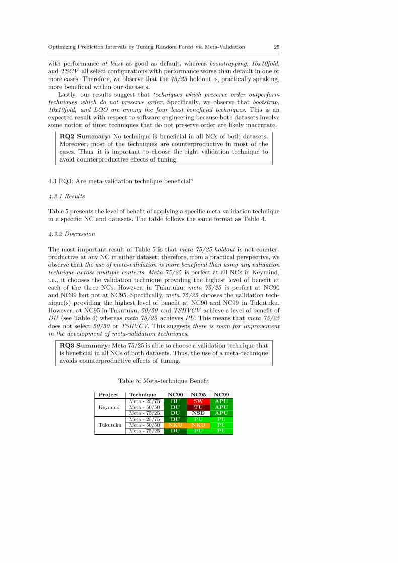
Table 5 presents the level of benefit of applying a specific meta-validation techniquein a specific NC and datasets. The table follows the same format as Table 4.

4.3.2 Discussion

The most important result of Table 5 is that meta 75/25 holdout is not counter-productive at any NC in either dataset; therefore, from a practical perspective, weobserve that the use of meta-validation is more beneficial than using any validationtechnique across multiple contexts. Meta 75/25 is perfect at all NCs in Keymind,i.e., it chooses the validation technique providing the highest level of benefit ateach of the three NCs. However, in Tukutuku, meta 75/25 is perfect at NC90and NC99 but not at NC95. Specifically, meta 75/25 chooses the validation tech-nique(s) providing the highest level of benefit at NC90 and NC99 in Tukutuku.However, at NC95 in Tukutuku, 50/50 and TSHVCV achieve a level of benefit ofDU (see Table 4) whereas meta 75/25 achieves PU. This means that meta 75/25does not select 50/50 or TSHVCV. This suggests there is room for improvementin the development of meta-validation techniques.

RQ3 Summary: Meta 75/25 is able to choose a validation technique thatis beneficial in all NCs of both datasets. Thus, the use of a meta-techniqueavoids counterproductive effects of tuning.

Table 5: Meta-technique Benefit

Project Technique NC90 NC95 NC99

KeymindMeta - 25/75 DU SW APUMeta - 50/50 DU TU APUMeta - 75/25 DU NSD APU

TukutukuMeta - 25/75 DU PU PUMeta - 50/50 NKU NKU PUMeta - 75/25 DU PU PU


5 Usability and Replicability

We have the right to use but not to share the Keymind and the Tukutuku datasets.Thus, we cannot allow exact replication of our study. However, in order to enhancethe study usability and replicability we developed and shared Meta tune3, an open-source Python package for constructing and analyzing prediction intervals. In orderto support the use of Meta tune, we provide a README5 and a demo4.

Meta tune currently provides five analysis operations:

1. Configuration coverage box-plots2. Configuration width box-plots3. Technique F1 and EMMRthe theE4. Tuning Benefit5. Meta-tuning Benefit

To support replicability we tried Meta tune on a very large open-source project,Apache Ant, as designed and collected by Jureczko and Madeyski [43] and avail-able online5. Tables 6 and 7 report the results of Meta tune on Apache Ant. TheREADME and the demo provide step-by-step instructions for running Meta tuneon Apache Ant and get results in Tables 6 and 7.

We note that results on Tables 6 and 7 are meant to be replicable but notgeneralize given that the data might not be designed and collected to support PIs.

Table 6: validation technique benefit in Ant

Technique NC90 NC95 NC99100 OOS Bootstrap NSD NSD DU10x10fold NSD NSD NKU25-75 NSD NSD DU50-50 NSD NSD DU75-25 NSD NSD DULOO NSD NSD NKUTSCV NSD NSD DUTSHVCV NSD NSD DU

Table 7: Meta-75/25 benefit in Ant

Technique NC90 NC95 NC99Meta-25/75 NSD NSD DUMeta-50/50 NSD NSD DUMeta-75/25 NSD NSD DU

3 https://github.com/smbayley/meta˙tune4 https://youtu.be/jer9mpcZCuo5 https://doi.org/10.5281/zenodo.268440


6 Threats to Validity

In this section, we report the threats to validity related to our study. The de-scription is organized by threat type, i.e., Conclusion, Internal, Construct, andExternal.

6.1 Conclusion

Conclusion validity regards issues that affect the ability to draw accurate conclu-sions about relations between the treatments and the outcome of an experiment[95].

We tested all hypotheses with nonparametric tests (e.g., Friedman) which areprone to type-2 error, i.e,. not rejecting a false hypothesis. We have been able toreject the hypotheses in most of the cases; therefore, the likelihood of a type-2error is low. Moreover, the alternative would have been using parametric tests(e.g., ANOVA) which are prone to type-1 error, i.e., rejecting a true hypothesis,which in our context is less desirable than type-2 error.

6.2 Internal

Internal validity regards the influences that can affect the independent variableswith respect to causality [95].

Results are related to the specific set of predictors used. We cannot check ifthese predictors are perfect. It could be that the set of predictors in use impactsthe benefit of validation or meta-validation. We tried our best when developingthe dataset (see Section 3.1.1 and Mendes et al. [58]) to include all predictors thatare reasonably correlated with number of post-defects. Moreover, the use of RFminimizes this threat because it performs feature selection intrinsically.

Lanza et al. [51] report on the the time-space continuum threats to validity invalidating recommendation systems based on past data. We believe this threat islow in the Keymind case since a prediction model was already in use when thereleases happened.

6.3 Construct

Construct validity regards the ability to generalize the results of an experiment tothe theory behind the experiment [95].

The use of three specific coverage levels (i.e., NC90, NC95 and NC99) mightinfluence our results. However we chose these coverage levels according to The-lin and Runeson [88] and the feedback of the analytic users, i.e., the Keyminddevelopers and project managers. Specifically, it does not make sense to spendresources to develop a tool that is desired to be accurate less than 90% of thetime. Therefore, we did not consider nominal confidences less than 90%. Lastly, a100% nominal confidence would have had increased the mean width by 55% com-pared to a 99% confidence (i.e., 17.7 vs 27.5), thus highly reducing the analyticactionability; therefore, we did not consider NC100.


Configuration goodness is dependent on context-specific goal(s). Certain orga-nizations might prioritize narrow intervals over reliable intervals. In this paper, wehad a specific goal in mind (i.e., to support the claim “I am NC% confident thatthe number of defects is between a and b”). We recognize that our results mightnot generalize to organizations with different goals, even if we do not know of anysuch organizations.

Moreover, the definition of the scenario tags as beneficial, neutral and coun-terproductive could be subjective. We defined and discussed the scenarios tags topragmatically represent the desire of the analytic users, i.e., the Keymind devel-opers and project managers.

Some might argue that a validation technique is beneficial if it selects the bestconfiguration rather than a configuration that is better than the default. However,understanding if a validation technique selects the best configuration is interestingto know if the question to answer is if a validation technique is perfect rather thanbeneficial. Anyway, we show that no validation technique and meta-validationtechnique is perfect and this paves the way to future research effort.

The default configuration might vary among implementations. The defaultMTRY for Sci-Kit Learn’s RF regressor is 1.0. However, the default MTRY in R’s6

implementation is n3 , where n is the number of predictors. The default MTRY in

WEKA’s implementation is log2(n) + 1 where n is the number of predictors. It ispossible that the benefit reported for tuning and meta-validation techniques variesamong different default configurations.

Mayr et al. [55] suggest that the only way to demonstrate PI correctness iswith an empirical evaluation based on simulated data (i.e., conditional coveragevs sample coverage). If true, this could limit the generalizability of our results.However, previous successful SE studies working with PIs have reported samplecoverage [1, 42] rather than conditional coverage, and thus our results fit intoexisting SE research.

6.4 External

External validity regards the extent to which the research elements (subjects,artifacts, etc.) are representative of actual elements [95].

This study used only two datasets and hence could be deemed of low general-ization compared to studies using tens or hundreds of datasets. However, as statedby Nagappan et al. [69], “more is not necessarily better.” We preferred to test ourhypotheses on datasets in which we were confident quality is high and that areclose to industry. Moreover, in order to encourage replicability, we have providedmeta-tune, an open source python package for using and tuning PIs.

Both Keymind and Tukutuku datasets are relatively large (363 and 195 indus-trial data points respectively). More common industry datasets could be smaller.Thus, we plan to investigate how the size of the dataset influences tuning andmeta-tuning accuracy.

Neither Keymind nor Tukutuku are open-source projects. Thus, our resultsmight not be generalizable to the context of open-source development.

6 http://lojze.lugos.si/ darja/software/r/library/randomForest/html/randomForest.html


The benefit of tuning or meta-validation techniques depends on the goodnessof the default configuration, i.e., if default is optimal there is no need to tune ormeta-tune. Thus, the observed tuning and meta-tuning benefits might not gen-eralize to datasets in which the default configuration is more frequently optimal.However, Provost [74] and Tosun and Bener [90] suggest the default configurationis suboptimal in many cases. Further, even if default is the best configuration,this study is valuable as it demonstrates meta-tuning can be used to minimize thepotential negative impact of tuning.

7 Conclusion

There are types of variables, such as those in defect and effort prediction, inwhich prediction intervals can provide more informative and actionable resultsthan point-estimates. The aim of this paper was to investigate the use and opti-mization of prediction intervals by automatically configuring Random Forest.

We have been inspired by the recent positive results of tuning in softwareengineering and in Random Forest. As detailed in Briand et al. [16], softwareengineering research made in collaboration with industry, such as this work, “doesnot attempt to frame a general problem and devise universal solutions, but rathermakes clear working assumptions, given a precise context, and relies on trade-offsthat make sense in such a context to achieve practicality and scalability.” As is thecase with any software engineering advance in industry, the presented research isimpacted by human, domain, and organizational factors. To support the creationof a body of knowledge on tuning and meta-validation, we provided a Pythonpackage for tuning and meta-validation of prediction intervals.

We tune Random Forest by performing an exhaustive search search with aspecific validation technique on a single Random Forest parameter since this isthe only parameter that is expected to impact prediction intervals. This paper in-vestigates which, out of eight validation techniques, are beneficial for tuning, i.e.,which automatically choose a Random Forest configuration constructing predic-tion intervals that are reliable and with a smaller width than the default configu-ration. Additionally, we present and validate three meta-validation techniques todetermine which are beneficial, i.e., those which automatically chose a beneficialvalidation technique. Our validation uses data from our industrial partner (Key-mind Inc.) and the Tukutuku Research Project, containing 363 and 195 industrialdata points related to post-release defect prediction and Web application effortestimation respectively. We focus validation on three nominal confidence levels(i.e., 90%, 95% and 99%), thus leading to six cases (three nominal confidences foreach dataset). Results show that: 1) The default configuration is unreliable in fivecases. 2) Previously successfully adopted validation techniques for tuning, such as50/50 holdout and bootstrap, fail to be beneficial and are counterproductive in atleast one case. 3) No single validation technique is always beneficial for tuning. 4)Most validation techniques are counterproductive at 95% confidence level. 5) Themeta 75/25 holdout technique selects the validation technique(s) that are bene-ficial in all cases. We note that these results are not meant to generalize to theentire machine learning domain. Rather, these results are specific to two industrialdatasets related to defect prediction and effort estimation.


To our knowledge, this is the first study to construct prediction intervals usingRandom Forest on software engineering data. Further, this is the first study toinvestigate meta-validation in the software engineering domain. As such, there issignificant room for future research. From a researcher’s perspective, there is roomfor improvement in the following areas.

1) Random Forest prediction intervals, as there are cases where no configurationis reliable.

– Distribution as inputs: we envision a model that accepts, as an input, a distri-bution of values, rather than a point-value [78].

– Adjusting intervals: we envision a mechanism, such as the one presented byKabaila and He [44], measuring the error of prediction intervals during trainingand using this measurements to adjust the intervals produced during testing.

– Heterogeneous forests: we would like to investigate the accuracy of a RandomForest in which the underlying decision trees have different configurations.

– Combining human and model estimates: Jørgensen and Moløkken [40] showthat human-estimates can be used to construct informative PIs. We wouldlike to incorporate human-based estimates into our construction of predictionintervals.

2) Validation and meta-validation techniques, as there are configurations that arebetter than the selected ones.

– Better tuning and meta-validation techniques: this study evaluated eight vali-dation techniques and three meta-validation techniques. These are large num-bers considering no previous study (that we know of) applied more than onevalidation technique and no meta-validation techniques. However, there aretechniques that we did not consider because they have not proven to be assuccessful, such as the non-repeated k-fold cross-validation.

– Meta-meta-validation: because meta-validation improved on tuning, it is in-teresting to investigate if meta-meta-validation improves on meta-validation,i.e., if we can automatically choose the meta-validation technique. However,the higher the level of meta evaluations, the smaller the training and testingdataset becomes, and hence the results will tend to become less generalizable.In other words, there is a point where “more meta” becomes counterproductive.We would like to investigate “what is the appropriate level of meta?”

– Impact of size and noise: Several studies investigate how size and noise im-pact defect classification accuracy [37, 46, 76]. On the same vein, we plan toinvestigate how size and noise impact the construction of narrow and reliableprediction intervals.

– Semi-automated decisions: on the one hand, we like to make decisions based onhistorical data rather than subjective opinions. In this study, we used tuningfor making decision about the configuration to use, and used meta-validationfor making decisions about the validation technique to use. On the other hand,data is rarely perfectly accurate or complete. Therefore, we need to develop abody of knowledge to understand when a parameter or a technique is likely tobe better than another.

From a practitioner’s perspective, we found the Random Forest to be a reliableapproach to construct prediction intervals. However, because the default configu-ration is frequently unreliable, the use of Random Forests must be accompanied


with an accurate tuning technique. Widely adopted validation techniques in tun-ing such as the 50/50 holdout and bootstrap were frequently counterproductive.Thus, we recommend practitioners to perform meta-validation to minimize thepossible counterproductive effects of tuning.

References

1. Lefteris Angelis and Ioannis Stamelos. A simulation tool for efficient analogybased cost estimation. Empirical software engineering, 5(1):35–68, 2000.

2. Lerina Aversano, Luigi Cerulo, and Concettina Del Grosso. Learning frombug-introducing changes to prevent fault prone code. In Ninth internationalworkshop on Principles of software evolution: in conjunction with the 6thESEC/FSE joint meeting, pages 19–26. ACM, 2007.

3. Ayse Bakır, Burak Turhan, and Ayse Bener. A comparative study for esti-mating software development effort intervals. Software Quality Journal, 19(3):537–552, 2011.

4. Claudia Beleites, Richard Baumgartner, Christopher Bowman, Ray Somorjai,Gerald Steiner, Reiner Salzer, and Michael G Sowa. Variance reduction in esti-mating classification error using sparse datasets. Chemometrics and intelligentlaboratory systems, 79(1):91–100, 2005.

5. Christoph Bergmeir and Jose M Benıtez. On the use of cross-validation fortime series predictor evaluation. Information Sciences, 191:192–213, 2012.

6. James S Bergstra, Remi Bardenet, Yoshua Bengio, and Balazs Kegl. Algo-rithms for hyper-parameter optimization. In Advances in Neural InformationProcessing Systems, pages 2546–2554, 2011.

7. Stefan Biffl. Using inspection data for defect estimation. IEEE Software, 17(6):36–43, 2000.

8. Stefan Biffl and Wilfried Grossmann. Evaluating the accuracy of defect esti-mation models based on inspection data from two inspection cycles. In Pro-ceedings of the 23rd International Conference on Software Engineering, pages145–154. IEEE Computer Society, 2001.

9. Barry Boehm, Chris Abts, and Sunita Chulani. Software development costestimation approachesa survey. Annals of software engineering, 10(1-4):177–205, 2000.

10. Markus Borg. Tuner: a framework for tuning software engineering tools withhands-on instructions in r. Journal of Software: Evolution and Process, 28(6):427–459, 2016.

11. Simone Borra and Agostino Di Ciaccio. Measuring the prediction error. acomparison of cross-validation, bootstrap and covariance penalty methods.Computational statistics & data analysis, 54(12):2976–2989, 2010.

12. Petronio L Braga, Adriano LI Oliveira, and Silvio RL Meira. Software effortestimation using machine learning techniques with robust confidence intervals.In Hybrid Intelligent Systems, 2007. HIS 2007. 7th International Conferenceon, pages 352–357. IEEE, 2007.

13. Ulisses M Braga-Neto and Edward R Dougherty. Is cross-validation valid forsmall-sample microarray classification? Bioinformatics, 20(3):374–380, 2004.

14. Leo Breiman. Random forests. Machine learning, 45(1):5–32, 2001.


15. Leo Breiman and Philip Spector. Submodel selection and evaluation in regres-sion. the x-random case. International statistical review/revue internationalede Statistique, pages 291–319, 1992.

16. Lionel Briand, Domenico Bianculli, Shiva Nejati, Fabrizio Pastore, andMehrdad Sabetzadeh. The case for context-driven software engineering re-search: Generalizability is overrated. Submitted to IEEE Software, 2017.

17. Lionel C Briand, Khaled El Emam, and Frank Bomarius. Cobra: a hybridmethod for software cost estimation, benchmarking, and risk assessment. InSoftware Engineering, 1998. Proceedings of the 1998 International Conferenceon, pages 390–399. IEEE, 1998.

18. Prabir Burman, Edmond Chow, and Deborah Nolan. A cross-validatorymethod for dependent data. Biometrika, pages 351–358, 1994.

19. G Campbell and Patroklos P Papapetrou. SonarQube in action. ManningPublications Co., 2013.

20. Mary Beth Chrissis, Mike Konrad, and Sandra Shrum. CMMI for develop-ment: guidelines for process integration and product improvement. PearsonEducation, 2011.

21. Terry Connolly and Doug Dean. Decomposed versus holistic estimates of effortrequired for software writing tasks. Management Science, 43(7):1029–1045,1997.

22. Anna Corazza, Sergio Di Martino, Filomena Ferrucci, Carmine Gravino, Fed-erica Sarro, and Emilia Mendes. Using tabu search to configure support vectorregression for effort estimation. Empirical Software Engineering, 18(3):506–546, 2013.

23. Sergio Di Martino, Filomena Ferrucci, Carmine Gravino, and Federica Sarro.A genetic algorithm to configure support vector machines for predicting fault-prone components. In International Conference on Product Focused SoftwareProcess Improvement, pages 247–261. Springer, 2011.

24. Matthew Doar. Practical JIRA Administration. ” O’Reilly Media, Inc.”, 2011.25. Yadolah Dodge. The Oxford dictionary of statistical terms. Oxford University

Press on Demand, 2006.26. Kaibo Duan, S Sathiya Keerthi, and Aun Neow Poo. Evaluation of simple

performance measures for tuning svm hyperparameters. Neurocomputing, 51:41–59, 2003.

27. Marco DAmbros, Michele Lanza, and Romain Robbes. Evaluating defect pre-diction approaches: a benchmark and an extensive comparison. EmpiricalSoftware Engineering, 17(4-5):531–577, 2012.

28. Stephen G Eick, Clive R Loader, M David Long, Lawrence G Votta, and ScottVander Wiel. Estimating software fault content before coding. In Proceedingsof the 14th international conference on Software engineering, pages 59–65.ACM, 1992.

29. Merran Evans, Nicholas Hastings, and Brian Peacock. Statistical distributions.2000.

30. Davide Falessi and Alexander Voegele. Validating and prioritizing quality rulesfor managing technical debt: An industrial case study. In Managing TechnicalDebt (MTD), 2015 IEEE 7th International Workshop on, pages 41–48. IEEE,2015.

31. Davide Falessi, Michele Shaw, and Kathleen Mullen. Achieving and main-taining cmmi maturity level 5 in a small organization. IEEE software, 31(5):


80–86, 2014.32. Jerome Friedman, Trevor Hastie, and Robert Tibshirani. The elements of

statistical learning, volume 1. Springer series in statistics Springer, Berlin,2001.

33. Wei Fu, Tim Menzies, and Xipeng Shen. Tuning for software analytics: Is itreally necessary? Information and Software Technology, 76:135–146, 2016.

34. Seymour Geisser. Predictive inference, volume 55. CRC press, 1993.35. Emanuel Giger, Marco D’Ambros, Martin Pinzger, and Harald C Gall.

Method-level bug prediction. In Proceedings of the ACM-IEEE internationalsymposium on Empirical software engineering and measurement, pages 171–180. ACM, 2012.

36. Lan Guo, Yan Ma, Bojan Cukic, and Harshinder Singh. Robust prediction offault-proneness by random forests. In Software Reliability Engineering, 2004.ISSRE 2004. 15th International Symposium on, pages 417–428. IEEE, 2004.

37. Kim Herzig, Sascha Just, and Andreas Zeller. It’s not a bug, it’s a feature:how misclassification impacts bug prediction. In Proceedings of the 2013 In-ternational Conference on Software Engineering, pages 392–401. IEEE Press,2013.

38. Tin Kam Ho. Random decision forests. In Document Analysis and Recognition,1995., Proceedings of the Third International Conference on, volume 1, pages278–282. IEEE, 1995.

39. Yue Jiang, Jie Lin, Bojan Cukic, and Tim Menzies. Variance analysis insoftware fault prediction models. In Software Reliability Engineering, 2009.ISSRE’09. 20th International Symposium on, pages 99–108. IEEE, 2009.

40. Magne Jørgensen and Kjetil Moløkken. Combination of software developmenteffort prediction intervals: why, when and how? In Proceedings of the 14thinternational conference on Software engineering and knowledge engineering,pages 425–428. ACM, 2002.

41. Magne Jørgensen and Dag I. K. Sjoeberg. An effort prediction interval ap-proach based on the empirical distribution of previous estimation accuracy.Information and Software Technology, 45(3):123–136, 2003.

42. Magne JøRgensen, Karl Halvor Teigen, and Kjetil MoløKken. Better surethan safe? over-confidence in judgement based software development effortprediction intervals. Journal of Systems and Software, 70(1):79–93, 2004.

43. Marian Jureczko and Lech Madeyski. Towards identifying software projectclusters with regard to defect prediction. In Proceedings of the 6th Interna-tional Conference on Predictive Models in Software Engineering, PROMISE’10, pages 9:1–9:10, New York, NY, USA, 2010. ACM. ISBN 978-1-4503-0404-7. doi: 10.1145/1868328.1868342. URL http://doi.acm.org/10.1145/

1868328.1868342.44. Paul Kabaila and Zhisong He. The adjustment of prediction intervals to ac-

count for errors in parameter estimation. Journal of Time Series Analysis, 25(3):351–358, 2004.

45. Sunghun Kim, E James Whitehead Jr, and Yi Zhang. Classifying softwarechanges: Clean or buggy? IEEE Transactions on Software Engineering, 34(2):181–196, 2008.

46. Sunghun Kim, Hongyu Zhang, Rongxin Wu, and Liang Gong. Dealing withnoise in defect prediction. In Software Engineering (ICSE), 2011 33rd Inter-national Conference on, pages 481–490. IEEE, 2011.

http://doi.acm.org/10.1145/1868328.1868342

http://doi.acm.org/10.1145/1868328.1868342


47. Ekrem Kocaguneli and Tim Menzies. Software effort models should be assessedvia leave-one-out validation. Journal of Systems and Software, 86(7):1879–1890, 2013.

48. Ron Kohavi et al. A study of cross-validation and bootstrap for accuracy es-timation and model selection. In Ijcai, volume 14, pages 1137–1145. Stanford,CA, 1995.

49. Stefan Kohler. Atlassian Confluence 5 Essentials. Packt Publishing Ltd, 2013.50. A Gunes Koru and Hongfang Liu. An investigation of the effect of module

size on defect prediction using static measures. In ACM SIGSOFT SoftwareEngineering Notes, volume 30, pages 1–5. ACM, 2005.

51. M. Lanza, A. Mocci, and L. Ponzanelli. The tragedy of defect prediction,prince of empirical software engineering research. IEEE Software, 33(6):102–105, Nov 2016. ISSN 0740-7459. doi: 10.1109/MS.2016.156.

52. Michele Lanza and Radu Marinescu. Object-oriented metrics in practice: usingsoftware metrics to characterize, evaluate, and improve the design of object-oriented systems. Springer Science & Business Media, 2007.

53. Stefan Lessmann, Bart Baesens, Christophe Mues, and Swantje Pietsch.Benchmarking classification models for software defect prediction: A proposedframework and novel findings. IEEE Transactions on Software Engineering,34(4):485–496, 2008.

54. P Li, Mary Shaw, and Jim Herbsleb. Selecting a defect prediction model formaintenance resource planning and software insurance. EDSER-5 affiliatedwith ICSE, pages p32–37, 2003.

55. Andreas Mayr, Torsten Hothorn, and Nora Fenske. Prediction intervals forfuture bmi values of individual children-a non-parametric approach by quantileboosting. BMC Medical Research Methodology, 12(1):6, 2012.

56. Nicolai Meinshausen. Quantile regression forests. Journal of Machine LearningResearch, 7(Jun):983–999, 2006.

57. Thilo Mende. Replication of defect prediction studies: problems, pitfalls andrecommendations. In Proceedings of the 6th International Conference on Pre-dictive Models in Software Engineering, page 5. ACM, 2010.

58. Emilia Mendes, Nile Mosley, and Steve Counsell. Investigating web size metricsfor early web cost estimation. Journal of Systems and Software, 77(2):157–172,2005.

59. Tim Menzies, JD Stefano, Kareem Ammar, Kenneth McGill, Pat Callis,J Davis, and R Chapman. When can we test less? In Software Metrics Sym-posium, 2003. Proceedings. Ninth International, pages 98–110. IEEE, 2003.

60. Tim Menzies, Zach Milton, Burak Turhan, Bojan Cukic, Yue Jiang, and AyseBener. Defect prediction from static code features: current results, limitations,new approaches. Automated Software Engineering, 17(4):375–407, 2010.

61. Tim Menzies, Andrew Butcher, Andrian Marcus, Thomas Zimmermann, andDavid Cok. Local vs. global models for effort estimation and defect prediction.In Automated Software Engineering (ASE), 2011 26th IEEE/ACM Interna-tional Conference on, pages 343–351. IEEE, 2011.

62. Tim Menzies, Andrew Butcher, David Cok, Andrian Marcus, Lucas Layman,Forrest Shull, Burak Turhan, and Thomas Zimmermann. Local versus globallessons for defect prediction and effort estimation. IEEE Transactions onsoftware engineering, 39(6):822–834, 2013.


63. Leandro Minku, Federica Sarro, Emilia Mendes, and Filomena Ferrucci. Howto make best use of cross-company data for web effort estimation? In EmpiricalSoftware Engineering and Measurement (ESEM), 2015 ACM/IEEE Interna-tional Symposium on, pages 1–10. IEEE, 2015.

64. Bharavi Mishra, K Shukla, et al. Defect prediction for object oriented softwareusing support vector based fuzzy classification model. International Journalof Computer Applications, 60(15), 2012.

65. Audris Mockus and David M Weiss. Predicting risk of software changes. BellLabs Technical Journal, 5(2):169–180, 2000.

66. Julie Moeyersoms, Enric Junque de Fortuny, Karel Dejaeger, Bart Baesens,and David Martens. Comprehensible software fault and effort prediction. J.Syst. Softw., 100(C):80–90, February 2015. ISSN 0164-1212. doi: 10.1016/j.jss.2014.10.032. URL http://dx.doi.org/10.1016/j.jss.2014.10.032.

67. Kjetil Molokken and Magen Jorgensen. A review of software surveys on soft-ware effort estimation. In Empirical Software Engineering, 2003. ISESE 2003.Proceedings. 2003 International Symposium on, pages 223–230. IEEE, 2003.

68. Ingunn Myrtveit, Erik Stensrud, and Martin Shepperd. Reliability and validityin comparative studies of software prediction models. IEEE Transactions onSoftware Engineering, 31(5):380–391, 2005.

69. Meiyappan Nagappan, Thomas Zimmermann, and Christian Bird. Diversityin software engineering research. In Proceedings of the 2013 9th joint meetingon foundations of software engineering, pages 466–476. ACM, 2013.

70. Ahmet Okutan and Olcay Taner Yıldız. Software defect prediction usingbayesian networks. Empirical Software Engineering, 19(1):154–181, 2014.

71. Frank Padberg. Empirical interval estimates for the defect content after aninspection. In Proceedings of the 24th International Conference on SoftwareEngineering, pages 58–68. ACM, 2002.

72. Hakan Petersson, Thomas Thelin, Per Runeson, and Claes Wohlin. Capture–recapture in software inspections after 10 years research—-theory, evaluationand application. Journal of Systems and Software, 72(2):249–264, 2004.

73. C Michael Pilato, Ben Collins-Sussman, and Brian Fitzpatrick. Version controlwith subversion. ” O’Reilly Media, Inc.”, 2008.

74. Foster Provost. Machine learning from imbalanced data sets 101. In Proceed-ings of the AAAI2000 workshop on imbalanced data sets, pages 1–3, 2000.

75. Jeff Racine. Consistent cross-validatory model-selection for dependent data:hv-block cross-validation. Journal of econometrics, 99(1):39–61, 2000.

76. Foyzur Rahman, Daryl Posnett, Israel Herraiz, and Premkumar Devanbu.Sample size vs. bias in defect prediction. In Proceedings of the 2013 9th jointmeeting on foundations of software engineering, pages 147–157. ACM, 2013.

77. Gunther Ruhe. Product release planning: methods, tools and applications. CRCPress, 2010.

78. Mehrdad Sabetzadeh, Davide Falessi, Lionel Briand, and Stefano Di Alesio.A goal-based approach for qualification of new technologies: Foundations, toolsupport, and industrial validation. Reliability Engineering & System Safety,119:52–66, 2013.

79. Federica Sarro, Alessio Petrozziello, and Mark Harman. Multi-objective soft-ware effort estimation. In Proceedings of the 38th International Conference onSoftware Engineering, pages 619–630. ACM, 2016.

http://dx.doi.org/10.1016/j.jss.2014.10.032


80. Shashank Mouli Satapathy, Barada Prasanna Acharya, and Santanu KumarRath. Early stage software effort estimation using random forest techniquebased on use case points. IET Software, 10(1):10–17, 2016. doi: 10.1049/iet-sen.2014.0122. URL https://doi.org/10.1049/iet-sen.2014.0122.

81. PA Selvaraj and Dr P Thangaraj. Support vector machine for software defectprediction. International Journal of Engineering & Technology Research, 1(2):68–76, 2013.

82. John Ferguson Smart. Jenkins-the definitive guide: Continuos integration forthe masses: also covers hudson., 2011.

83. Jasper Snoek, Hugo Larochelle, and Ryan P Adams. Practical bayesian opti-mization of machine learning algorithms. In Advances in neural informationprocessing systems, pages 2951–2959, 2012.

84. Muhammad Dhiauddin Mohamed Suffian and Suhaimi Ibrahim. A predictionmodel for system testing defects using regression analysis. arXiv preprintarXiv:1401.5830, 2014.

85. Chakkrit Tantithamthavorn, Shane McIntosh, Ahmed E Hassan, and KenichiMatsumoto. Automated parameter optimization of classification techniquesfor defect prediction models. In Proceedings of the 38th International Confer-ence on Software Engineering, pages 321–332. ACM, 2016.

86. Chakkrit Tantithamthavorn, Shane McIntosh, Ahmed E Hassan, and KenichiMatsumoto. An empirical comparison of model validation techniques for defectprediction models. IEEE Transactions on Software Engineering, 43(1):1–18,2017.

87. Thomas Thelin. Team-based fault content estimation in the software inspec-tion process. In Software Engineering, 2004. ICSE 2004. Proceedings. 26thInternational Conference on, pages 263–272. IEEE, 2004.

88. Thomas Thelin and Per Runeson. Confidence intervals for capture–recaptureestimations in software inspections. Information and Software Technology, 44(12):683–702, 2002.

89. Chris Thornton, Frank Hutter, Holger H Hoos, and Kevin Leyton-Brown.Auto-weka: Combined selection and hyperparameter optimization of classi-fication algorithms. In Proceedings of the 19th ACM SIGKDD internationalconference on Knowledge discovery and data mining, pages 847–855. ACM,2013.

90. Ayse Tosun and Ayse Bener. Reducing false alarms in software defect predic-tion by decision threshold optimization. In Empirical Software Engineeringand Measurement, 2009. ESEM 2009. 3rd International Symposium on, pages477–480. IEEE, 2009.

91. Burak Turhan, Tim Menzies, Ayse B Bener, and Justin Di Stefano. On therelative value of cross-company and within-company data for defect prediction.Empirical Software Engineering, 14(5):540–578, 2009.

92. Scott A Vander Wiel and Lawrence G. Votta. Assessing software designs usingcapture-recapture methods. IEEE Transactions on Software Engineering, 19(11):1045–1054, 1993.

93. Peter A. Whigham, Caitlin A. Owen, and Stephen G. Macdonell. A baselinemodel for software effort estimation. ACM Trans. Softw. Eng. Methodol.,24(3):20:1–20:11, May 2015. ISSN 1049-331X. doi: 10.1145/2738037. URLhttp://doi.acm.org/10.1145/2738037.

https://doi.org/10.1049/iet-sen.2014.0122

http://doi.acm.org/10.1145/2738037


Table 8: Keymind predictors with evidence of impacting defectiveness

Predcitor Definition RationaleProject Age The duration, in days, from

the start of the first releaseto the start of the current re-lease.

More mature projects areless likely to be defect pronethan new projects [27].

Number of Devel-opers

The number of unique de-velopers that made a SVNcommit during the release.

Releases with more develop-ers are more likely to be de-fect prone [27].

Number of NewDevelopers

The number of unique de-velopers that made a SVNcommit during the currentrelease and had not made acommit during any previousrelease.

Releases with more new de-velopers are more likely tobe defect prone [27].

Prior Number ofGod Classes

The number of god classesthat were present in theproject at the end of the pre-vious release.

Projects with more godclasses are more likely to bedefect prone [27].

Project Architec-ture

A categorical feature thatspecifies the type of project(e.g., .NET standard vsMVC standard)

Some project architecturesrequire more developersand/or code to complete arequirement.

94. Ian H Witten, Eibe Frank, Mark A Hall, and Christopher J Pal. Data Mining:Practical machine learning tools and techniques. Morgan Kaufmann, 2016.

95. Claes Wohlin, Per Runeson, Martin Hst, Magnus C. Ohlsson, Bjrn Regnell, andAnders Wessln. Experimentation in Software Engineering. Springer PublishingCompany, Incorporated, 2012. ISBN 3642290434, 9783642290435.

96. Feng Zhang, Audris Mockus, Iman Keivanloo, and Ying Zou. Towards build-ing a universal defect prediction model. In Proceedings of the 11th WorkingConference on Mining Software Repositories, pages 182–191. ACM, 2014.

97. Thomas Zimmermann, Rahul Premraj, and Andreas Zeller. Predicting defectsfor eclipse. In Proceedings of the third international workshop on predictormodels in software engineering, page 9. IEEE Computer Society, 2007.

Appendix

We divide the Keymind predictors in two groups: predictors having prior studiessupporting their impact on defectiveness and predictors that are intuitively corre-lated with defectiveness. Tables 8 and 9 present the names and information abouteach of the selected predictors.


Table 9: Keymind predictors that are intuitively correlated with defectiveness

Predictor Definition IntuitionDevelopment Du-ration

The duration, in days, fromthe start of the releases tothe end of the releases

Longer durations are indica-tive of releases with morerequirements, and hence re-leases that are more defectprone. Moreover, shorter du-rations with a high numberof features are more defectprone.

Estimated Effort The total estimated effort,in hours, required for devel-opment.

More estimated effort isindicative of releases withmore complex features, andhence releases that are moredefect prone.

Testing Time The total amount of time,in hours, spent on internaltesting.

More time spent testing re-veals defects prior to release,and hence makes releasesless defect prone.

Number of ChangeRequests

The number of JIRA tasksthat specify a change to theimplementation of a previ-ously specified requirement.

More change requests areindicative of releases withmore development, andhence releases that are moredefect prone.

Number of Imple-mentation Tasks

The number of JIRA tasksthat specify implementationof a new requirement.

More implementation tasksare indicative of releaseswith more development, andhence releases that are moredefect prone.

Number of ReleaseCandidates

The number of internal re-leases before the external re-lease.

More release candidates isindicative of releases thathave been exposed to moreinternal use, and hence re-leases that are less defectprone.

Number of Users The number of end-users. More end-users is indicativeof releases that will be ex-posed to more external use,and hence releases that aremore defect prone.

optimizing prediction intervals by tuning random forest ... · meta-validation for tuning...

Documents