OPTIMIZING PARAMETERS OF MACHINE LEARNING ALGORITHMS

Seminar I

Valentin Koblar

Supervisor: Prof. Bogdan Filipič

Approved by supervisor: _____________________

(signature)

Study programme: Information and Communication Technologies

Doctoral degree

Ljubljana, 2012

Abstract

Machine learning algorithms require setting of parameters for achieving high-quality results. Manual parameter setting and searching for optimal parameter values based on learning and experience can be very time-consuming. Using optimization algorithms, we can get good parameter settings and save time. In our research, we used the multiobjective optimization algorithm called DEMO to optimize the parameters of a machine learning algorithm. DEMO is an extension of differential evolution which is a simple but powerful singleobjective optimization algorithm. We optimized the parameters of the J48 algorithm for building decision trees, considering two criteria, the size and the accuracy of decision trees. Optimization results on three industrial domains show that DEMO can successfully set parameter values for building nondominated decision trees.

Key words: machine learning, decision tree, classification accuracy, decision tree size, machine learning algorithm parameters, multiobjective optimization, differential evolution, DEMO

TABLE OF CONTENTS

1. INTRODUCTION ............................................................................ 1

2. PROBLEM DEFINITION ..................................................................... 1

2.1. Machine learning ..................................................................... 2

2.2. Multiobjective optimization ........................................................ 3

3. RELATED WORK ............................................................................ 5

4. TEST ENVIRONMENT ....................................................................... 6

4.1. Building decision trees with the J48 algorithm .................................. 7

4.2. Differential evolution for multiobjective optimization (DEMO) ............... 7

5. EXPERIMENTS AND RESULTS.............................................................. 9

5.1. Test problems......................................................................... 9

5.2. Results ................................................................................ 11

6. CONCLUSION .............................................................................. 13

7. LITERATURE ............................................................................... 15

APPENDIX ....................................................................................... 17

1

1. INTRODUCTION

In practice we constantly face the needs for optimization. Optimization can be defined as finding the most suitable solution to a given problem under certain circumstances. Every day, almost unconsciously, we optimize our routes and activities. However, we have to deal with much more complex optimization problems, such as optimal distribution of products on production lines in factories where the objective is to fulfil the orders.

Particularly challenging are multiobjective optimization problems. In multiobjective optimization, as the name implies, one has to consider several objectives at the same time. These are often in contradiction, meaning that improving solutions with respect to one objective deteriorates them with respect to others. In such cases, there is not a single optimal solution, but a set of solutions, which represent tradeoffs among the given criteria. Usually there are no exact methods for solving these kind of problems. Therefore, when considering multiobjective optimization, we commonly use stochastic optimization methods.

Stochastic optimization methods use algorithms with certain steps based on randomness. The consequences of randomness are various results obtained in multiple runs of an algorithm. In our work, we were particularly interested in evolutionary optimization algorithms, more specifically in differential evolution, the inspiration for which comes from biological evolution. Using an evolutionary optimization algorithm on selected domains we were able to show that these algorithms are suitable for solving multiobjective optimization problems and effectively solve optimal parameter settings problem in machine learning algorithms.

2. PROBLEM DEFINITION

The primary goal of machine learning algorithms is autonomous building of models from the selected database. Generally, machine learning algorithms do not provide optimal results without being properly tuned. For building models of high classification accuracy and, at the same time, understandability, it is not only necessary to choose an appropriate machine learning algorithm but also requires time-consuming setting of algorithm parameters.

Most machine learning algorithm practitioners do not use optimization methods for setting the algorithm parameters. There are guidelines and recommendations which define frameworks for setting machine learning algorithms parameters and are used for initial parameter setup. However, most user use manual parameter setting or grid search for appropriate parameter values.

Manual tuning of parameters and finding high-quality parameter settings of a machine learning algorithm can be very time-consuming, especially when the learning algorithm involves a large number of parameters. This requires excellent knowledge of algorithms and properties of the learning domain. In addition, the solutions obtained by manual settings are usually not equally distributed in the objective space.

2

A possible approach for setting parameter values of machine learning algorithms is grid search. With this method, one predefines discrete values of the parameters. A computer algorithm then systematically searches and evaluates decision models, built by using the predefined values of machine learning algorithm parameters.

Grid search is a computationally demanding process: by increasing the number of parameters and reducing the interval between discrete values, the number of possible combinations increases exponentially. The problem of a large number of calculations can be solved by parallel computing on multicore computers or by employing the cloud computing techniques. This method has proven to be more effective and efficient than manual search, as it provides more accurate decision models in shorter time [7].

Another possible approach to finding appropriate parameter settings of machine learning algorithms is using optimization methods. The problem of parameter tuning for machine learning algorithms can be defined as an optimization problem. Its objective function can be defined as a classification accuracy of the designed model, which is to be maximized, the complexity of the built model, which is to be minimized, etc. Considering more than one objective function leads to a multiobjective optimization problem which is generally more complex to solve than a singleobjective problem. This approach requires more programming, but it turns to be the most appropriate, especially in complex domains [17].

2.1. Machine learning

The field of machine learning, according to the type of input data, the method of learning and the purpose of designed models, includes a set of algorithms. In this work, we were focused on the problem of classification of instances from a certain domain into appropriate classes. From machine learning perspective, classification can be defined as search for a function that maps the space of attributes of the domain to the target classes. The most widespread classification algorithms are algorithms for building decision trees. Decision trees are very frequently used for classification, as they are easy to use and understand.

There are usually two criteria for the quality of decision trees: classification accuracy and decision tree size (often expressed as the number of nodes in the tree).

With the increasing size of the decision tree its incomprehensibility also increases, which is particularly undesirable if the decision tree is used for the interpretation of the discovered relationships in the training data. If a decision tree is used for classification, its size it is not so significant, as the implementation of decision trees in practice is not demanding. Smaller trees are often preferred to larger ones, as they do not overfit the training set and are less sensitive to noise.

The size of decision trees can be controlled during the construction process by pruning. There are two approaches to decision tree pruning: prepruning (terminating the subtree construction during the tree-building process) and postprunning (pruning the subtrees of an already constructed tree).

3

The key goal of decision trees is classification of previously unseen instances from a specific domain into appropriate classes. The classification accuracy is the proportion of correctly classified instances in a given set of instances. If a decision tree would have been based on all available instances, its classification accuracy determined in this way would not be representative. Therefore, a decision tree is built on a subset of all available data, called the learning set. The remaining data are used to assess the accuracy of the built classification tree and is called the test set. To avoid dividing sensitive information between the learning set and the test set, the procedure is repeated n times, where the test set is one of the n parts of the data set and the rest is used for the learning set. This method is called n-fold cross-validation.

In building decision trees, we are interested in two criteria: the accuracy of the classification tree and its size. This is a typical multiobjective, more specifically biobjective optimization problem.

2.2. Multiobjective optimization

Multiobjective optimization enables simultaneous optimization of several functions. These are often in contradiction, which means that improving solutions with respects to one criterion makes them worse with respect to others. Therefore, multiobjective optimization is more complex than singleobjective. In order to compare solutions in multiobjective optimization with each other, we utilize the dominance relations. One solution dominates another solution, if at least in one objective is better than the other, and at the same time not worse in other objectives. Figure 1 shows an example of mapping from the decision space to the objective space. The solution a dominates solutions b and c (assuming that both objectives are being minimized).

Figure 1: The concept of dominance shown for a biobjective function f

With respect to dominance relation, solutions may also be incomparable. In Figure 1, solutions e and d are incomparable. The set of all nondominated feasible solutions in the entire objective space is called nondominated or Pareto optimal front. To choose one solution from the Pareto optimal front, we need additional information about the importance of criteria.

DECISION SPACE OBJECTIVE SPACE

4

Usually, the goal of optimization is to provide one optimal solution. Figure 2 shows two possible approaches to determining one optimal solution in multiobjective optimization [15].

Figure 2: Preference based and ideal approaches to multiobjective optimization

In the preference-based approach, the multiobjective optimization problem is first transformed into a singleobjective one, according to some preference for the objectives. This can be achieved by combining the objectives using a weighted sum. With this method we define weights which indicate the importance of objectives in advance. The optimization problem is then solved in the singleobjective manner. The result is one solution for a particular optimization problem. The main disadvantage of the preference-based approach is the requirement to know the importance of objectives, which is not always possible. The solution acquired this way depends on the weights used to transform the multiobjective problem into a singleobjective one.

In the ideal approach, we find a set of nondominated solutions with the multiobjective optimization algorithm first and only then the preference information is used to select a single solution among several alternatives. The ideal principle does not demand the user to set a preference for the objectives in advance. The user chooses the preferred one among several tradeoff solutions. This approach is less subjective than the preference-based approach, but on the other hand it is more computationally demanding. The goal of the ideal approach is to find a set of Pareto optimal solutions which are equally distributed along the front. Implementation of ideal approach was only made possible with the development of population-based search algorithm, such as the evolutionary algorithms.

In this work we use the ideal approach as our objective is to enable the user to choose the most appropriate solution to serve his/her needs.

PREFERENCE-BASED APPROACH IDEAL APPROACH

5

3. RELATED WORK

Motivation for this research results from our previous work on solving an industrial machine learning problem [10]. Decision trees were built from a set of instances, optimizing the classification accuracy and the size of decision trees. The values of machine learning algorithm parameters were varied manually, which enabled us to build decision trees of various classification accuracy and size.

A step forward in solving this problem was made in [13]. Here we built several decision trees, employing the DEMO algorithm (Differential Evolution for Multiobjective Optimization) [17] in connection with a machine learning algorithm. These decision trees were distributed along the nondominated front. It turned out that this problem was not so computationally complex, hence the resulting decision trees had high classification accuracy and were rather small at the same time.

Several authors have already worked on machine learning algorithm parameter optimization. Kohavi and John [11] were searching for suitable parameter settings of the C4.5 algorithm for building decision trees. Their method was based on exploring parameter values, while the accuracy was measured through 10-fold cross-validation. They performed experiments on 33 datasets. Results have shown that optimized parameter values in most cases give identical or better results than default parameter settings. It should be noted that the problem was treated as singleobjective where the only function was classification accuracy.

Similar experiments were performed by Mladenić [12] who searched for optimal settings of the parameter value for decision tree postprunning. The optimization objective was the accuracy of the decision tree estimated with 10-fold cross-validation. The decision space was explored using various learning algorithms. The tests on different datasets showed comparable results of the applied algorithms.

Bohanec and Bratko [3] presented the OPT algorithm which systematically explores the space of possible solutions. Each decision tree found has the highest accuracy among all possible pruned trees of the same size. Although this algorithm gives very good results, it has certain disadvantages. Systematically building all possible decision trees and keeping the best ones is a time-consuming process.

There are not many publications on parameter optimization for decision tree building algorithms. The following paragraphs provide an overview of the work in parameter optimization for other machine learning algorithms.

Bergstra et al. [2] studied algorithms for setting parameter values of neural networks. They used two methods: random search and the algorithm called TPE (Tree-structured Parzen Estimator). The methods were tested on the same domain. The authors also compared the classification accuracy of built models after a certain number of the optimization algorithm runs. They discovered that their algorithm TPE builds models with higher classification accuracy significantly faster in comparison to random search.

Several authors were dealing with parameter optimization of the SVM (Support Vector Machine) algorithm. Rossi and De Carvalho [16] compared four algorithms to optimize the SVM parameters: genetic algorithm, clonal selection algorithm, ant colony optimization algorithm and particle swarm optimization. Optimization of the SVM parameters was performed on four different domains. Optimization results were varying and depending on the chosen domain. In some cases the SVM

6

algorithm with default parameters was even more successful than the SVM algorithm with optimized parameters.

Lessmann, Stahlbock and Crone [8] optimized parameters of the SVM algorithm by using a genetic algorithm. The method was tested on one dataset. Results from this test were compared to results of grid search algorithm. They discovered that setting parameters with genetic algorithms is more efficient and gives more repeatable results.

Almeida and Ludermir [1] used the evolutionary algorithm to automatically set the parameters of neural networks. They developed an algorithm GANNTune (Genetic Algorithm + Artificial Neural Network + Tuning) and tested it on three different domains. In comparison to similar algorithms GANNTune algorithm proved to be very efficient. Its classification accuracy was higher on all three domains.

Leung et al. [9] developed a genetic algorithm for setting the parameter values of neural networks. Experiments were made on six test mathematical functions. Task of genetic algorithm was to found global maximum. In comparison to classic genetic algorithm, the proposed genetic algorithm was significantly more efficient. Algorithm required smaller number of generations for finding maximum of predefined functions. The algorithm was also tested on the problem of setting parameter values in neutral networks. Neutral networks, based on data of the solar activity from the past years, were used for predicting the number of sunspots in the next period. Neural networks, in combination with genetic algorithm, were proved to be very effective and accurate.

4. TEST ENVIRONMENT

The first step, before testing the optimization method on learning domains, was to set up test environment. To build decision trees, we used the software environment Weka [18]. Weka was connected with multiobjective optimization algorithm DEMO (Differential Evolution for Multiobjective Optimization) [17]. DEMO is based on differential evolution and can be used for solving numerical multiobjective optimization problems. A schematic representation of a test environment is shown in Figure 3.

DEMO starts with a population of random machine learning parameter values. The machine learning algorithm based on these parameter values builds a decision tree with certain classification accuracy and size. In the next step, DEMO compares the resulting solution (candidate) to previous solutions (parents). If the candidate is better than or equal to the parent, the candidate is added to the population. Otherwise the candidate is discarded. The procedure is repeated until the stopping criterion is met.

7

Figure 3: Schematic representation of machine learning algorithm parameter optimization

4.1. Building decision trees with the J48 algorithm

In the Weka software environment, we focused on the algorithm for decision tree building C4.5, more exactly on its implementation in Weka known as J48. This machine learning algorithm enables us to set more than ten parameters which have influence on resulting decision tree. Table 1 shows five parameters that were optimized in our work.

Table 1: Parameters of the J48 machine learning algorithm used in optimization

Parameter Possible values Default value

M – minimum number of instances in a leaf 1,2,... 2 U – use of unpruned trees yes/no no C – confidence factor used in postpruning [0.001, 0.5] 0.25 S – subtree raising operation in postpruning yes/no yes B – use of binary splits yes/no no

The classification accuracy was measured by using 10-fold cross-validation. As Table 1 suggests, there are many possible combinations of parameter values. Manually setting and searching for optimal parameter values would be very time-consuming.

4.2. Differential evolution for multiobjective optimization (DEMO)

DEMO is a differential evolution algorithm adapted for multiobjective optimization. The advantage of differential evolution is in its ease of implementation and use. Differential evolution starts with a population of random solutions from which in

optimization algorithm

DEMO

parameter space

machine learning algorithm WEKA

parameter settings

machine learning

results

results

evaluation

learning domain

parameter

settings quality

optimized

parameter settings

8

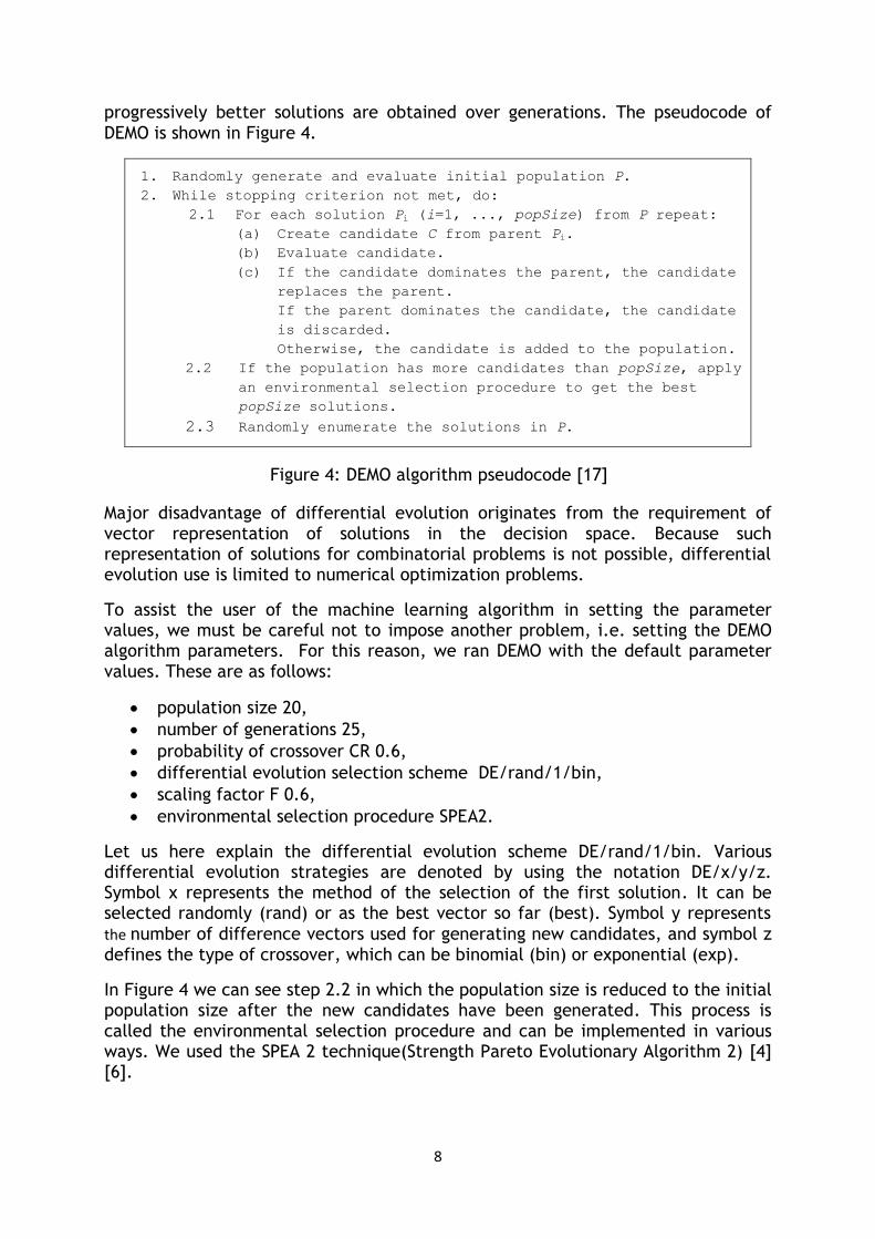
progressively better solutions are obtained over generations. The pseudocode of DEMO is shown in Figure 4.

1. Randomly generate and evaluate initial population P.

2. While stopping criterion not met, do:

2.1 For each solution Pi (i=1, ..., popSize) from P repeat:

(a) Create candidate C from parent Pi.

(b) Evaluate candidate.

(c) If the candidate dominates the parent, the candidate

replaces the parent.

If the parent dominates the candidate, the candidate

is discarded.

Otherwise, the candidate is added to the population.

2.2 If the population has more candidates than popSize, apply

an environmental selection procedure to get the best

popSize solutions.

2.3 Randomly enumerate the solutions in P.

Figure 4: DEMO algorithm pseudocode [17]

Major disadvantage of differential evolution originates from the requirement of vector representation of solutions in the decision space. Because such representation of solutions for combinatorial problems is not possible, differential evolution use is limited to numerical optimization problems.

To assist the user of the machine learning algorithm in setting the parameter values, we must be careful not to impose another problem, i.e. setting the DEMO algorithm parameters. For this reason, we ran DEMO with the default parameter values. These are as follows:

population size 20,

number of generations 25,

probability of crossover CR 0.6,

differential evolution selection scheme DE/rand/1/bin,

scaling factor F 0.6,

environmental selection procedure SPEA2.

Let us here explain the differential evolution scheme DE/rand/1/bin. Various differential evolution strategies are denoted by using the notation DE/x/y/z. Symbol x represents the method of the selection of the first solution. It can be selected randomly (rand) or as the best vector so far (best). Symbol y represents

the number of difference vectors used for generating new candidates, and symbol z defines the type of crossover, which can be binomial (bin) or exponential (exp).

In Figure 4 we can see step 2.2 in which the population size is reduced to the initial population size after the new candidates have been generated. This process is called the environmental selection procedure and can be implemented in various ways. We used the SPEA 2 technique(Strength Pareto Evolutionary Algorithm 2) [4] [6].

9

5. EXPERIMENTS AND RESULTS

Optimization of the J48 algorithm parameters with DEMO was performed on three learning domains. All three domains originate from industry. The first domain, commutators, has already been used for building decision trees in our previous work [10] [13]. Domain addresses the problem of quality assurance in graphite semiproduct treatment in the Kolektor company.

The second domain, emulsion, refers to maintaining the quality of emulsion in the process of steel rolling. It was obtained from the Acroni steel plant, Jesenice [5]. Here the task was to classify the emulsion quality into one of five quality classes.

The third domain, steel plates, was obtained from the UCI repository [14]. Data in this domain relates to the quality of produced steel plates. The task was to classify steel plates into one of the quality classes that describe type of faults.

In Subsection 5.1 we describe in detail each of the three domains, their attributes and classes. In Subsection 5.2 we present the results of the machine learning algorithm parameter optimization.

5.1. Test problems

Domain commutators included attributes of 509 graphite semiproducts. The graphite semiproduct is an integral part of the commutator, which is mounted on the rotor of the commutator motor. Plasma treatment of graphite semiproducts is one of the first processes in production of graphite commutators. The result of plasma treatment is the surface of the graphite semiproduct, appropriate for further processing. A problem appearing in this process is unstable surface treatment of graphite semiproducts. The differences in the surface treatment quality originate from inhomogeneity of graphite material and variations in the plasma treatment process. Each graphite semiproduct was described by eight attributes and it was classified into one of four possible quality classes. Quality classes and their distribution are shown in Table 2.

Attributes were extracted from digital images of the graphite semiproducts captured under 115-fold magnification with a digital microscope and processed with a computer vision algorithm. The attributes describing the semiproducts based on the captured images were the following: mean grayscale value, proportion of the most frequent grayscale value, standard deviation of the mean grayscale value, number of concaves on the captured image, proportion of concaves on the captured image, area of the smallest concave on the captured image, area of the largest concave on the captured image and the coloring. All attributes were numerical.

Table 2: Characteristics of the commutators learning domain

Class Number of examples Distribution of classes [%]

insufficiently treated 97 19.1

well treated 204 40.1

over-treated 99 19.4

colored 109 21.4

10

Total 509 100.0

The emulsion domain is from steel industry. Data were obtained in the process of steel cold rolling. In this process the generated heat must be dissipated by the cooling system. The cooling system uses the oil emulsion as a cooling medium. The quality of emulsion has essential effect on the quality of produced steel strips.

Consequently, the quality of emulsion should be continuously monitored and in the case of poor quality an appropriate action should be taken to improve its quality.

This domain contained 108 measurements of emulsion quality. Each measurement consisted of seven attributes, which are important for the emulsion quality. These attributes were: the saponification value, quantity of iron in the emulsion, quantity of iron in the emulsion sediment, concentration of oil in the emulsion, quantity of inactive oil in the emulsion, quantity of daily added oil, and quantity of daily added base. The first five attributes were numerical and the last two were categorical.

The task of machine learning was to build a classification model to classify the emulsion in the appropriate quality class. Characteristics of this domain are summarized in Table 3.

Table 3: Characteristics of the emulsion learning domain

Class Number of examples Distribution of classes [%]

excellent 6 5.5

great 20 18.5

ok 53 49.1

acceptable 27 25.0

bad 2 1.9

Total 108 100,0

Data from the steel plates domain were obtained from the UCI repository [14]. This domain contained data of failures in the production of steel plates. It contained 1941 learning examples described by 27 attributes. These attributes describe physical properties of steel plates, such as defect size, position of fault, light reflectance of the surface, material type, etc. All attributes were numeric.

Table 4: Characteristics of the steel plates learning domain

Class Number of examples Distribution of classes [%]

Pastry 158 8.1

Z_scratch 190 9.8

K_scratch 391 20.1

Stains 72 3.7

Dirtiness 55 2.8

Bumps 402 20.8

Other faults 673 34.7

Total 1941 100.0

11

The task of machine learning algorithm was to classify individual learning example into the appropriate class, type of fault. Classification classes of domain steel plates are shown in Table 4.

5.2. Results

Firstly, we built decision trees on selected domains with the default parameter settings of the J48 algorithm. Default parameter values are shown in Table 1. Decision trees built with the default parameter values, were compared with trees built with optimized parameters. Result of parameter optimization is not just one decision tree, but a set of nondominated decision trees. Nondominated front of decision trees and a decision tree built with the default parameter values are shown in Figure 5. This figure represents the result of a single run of the DEMO optimization algorithm.

Nondominated front for domain commutators consists of only four decision trees. Considering the number of attributes in this domain, the number of nondominated solutions found is relatively small. Knowing the background of this domain, we can claim, that the only solution applicable in practice is the one with the highest classification accuracy which is equal to 98.4 %. This classification accuracy is similar to the classification accuracy of the decision tree built with the default parameter values, but the size of the decision tree built with optimized parameter values is smaller. By optimizing the parameters, we therefore reduced the size of decision tree providing almost equal classification accuracy.

The decision tree built on the emulsion domain with default parameter values has the size of 25 and classification accuracy of 72.2 %. Comparison of this solution and the nondominated front of decision trees, built with optimized parameter values shows that smaller decision trees achieve equivalent or even higher classification accuracy. The decision tree of size 13 achieves classification accuracy of 75.0 %. On the emulsion domain DEMO achieved very good results.

Domain steel plates was the most complex domain regarding the number of learning examples and the number of attributes. Like in other two domains, optimizing machine learning algorithm parameters provided good results. By optimizing the parameters, we were able to build smaller decision trees with equivalent or higher classification accuracy, compared with the decision tree built with default parameter values.

Figure 5 shows the nondominated front generated in one run of DEMO. To confirm the repeatability of the results, we performed several runs of the optimization algorithm on each domain. As a measure of repeatability we used the hypervolume indicator. Hypervolume is defined as an area between nondominated front and the reference point in the objective space.

12

Figure 5: Results of decision tree building using default parameter values and optimized parameter values of the J48 machine learning algorithm

Figure 6 shows the improvement of hypervolume over five runs of the optimization algorithm on domain steel plates. As can be seen, hypervolume in all runs

13

converges to the same value. This means that the nondominated front of solutions is located in similar position, which proves the repeatability of the results.

Figure 6: Hypervolume improvement in five runs of the optimization algorithm on domain metal sheet

We also analyzed the optimized parameters of the machine learning algorithm. All nondominated solutions found on all three domains are listed in Tables 5-7 in Appendix. On domains commutators and emulsion the optimization algorithm found less nondominated solutions than the population size. We empirically confirmed the well-known fact that different parameter settings of a machine learning algorithm result in the same decision tree. On the more complex domain steel plates, all found solutions were nondominated. The used population size (20 solutions) was appropriate in terms of representativeness of the obtained approximation set. However, if the population size would be sufficiently large, the result of the machine learning algorithm would be the same – subsets of solutions, which differ in the decision space. Their mapping to the objective space results in the same solution.

Optimizing parameters of the machine learning algorithm on selected domains has proven to be effective. Parameter optimization is especially effective on complex domains, such as steel plates in our case. Implementation of optimized decision trees is straightforward and very efficient in terms of the number of the required attribute tests, which may be very beneficial from the practical point of view.

6. CONCLUSION

The use of machine learning algorithms in practice is increasing. A user of a machine learning algorithm has to have knowledge of machine learning algorithms and be familiar with the domain for which classification models are being built. Certain parameters have to be set for every machine learning algorithm. These parameters can have major influence on the result of machine learning.

14

Optimization methods can be used to help finding optimal parameter settings. Consequently, the user can focus on the results of machine learning rather than on finding optimal parameter values.

In this work we dealt with decision tree building, more precisely with the J48 algorithm implemented in the Weka software environment. To optimize the J48 parameters, we used the DEMO multiobjective optimization algorithm which is based on differential evolution. DEMO is a simple and powerful optimization algorithm, but its use is limited to numerical optimization problems.

Optimization of machine learning algorithm parameters was performed on three industrial domains. The results show, that algorithmic parameter optimization in comparison to manual search for appropriate parameter settings is much more effective. The machine learning algorithm with optimized parameter values managed to build simplified decision trees with higher classification accuracy on all three domains. Optimization with the DEMO algorithm, despite of its stochastic nature, has proved to be reliable, since DEMO achieved similar results in multiple runs.

In our future work we will test the optimization approach on more complex domains, containing higher number of learning examples and attributes. We will in detail analyze the results in decision space (various parameter settings of the machine learning algorithm that generate same decision trees) and in objective space (regarding the presence of classes in decision trees). The described optimization approach can be extended to other machine learning algorithms and can account for additional optimization objectives.

15

7. LITERATURE

[1] Almeida L. M., Ludermir T. B. Tuning artificial neural Networks Parameters Using an Evolutionary Algorithm. Proceedings of the 8th International Conference on Hybrid Intelligent Systems, 2008, pages 927-930.

[2] Bergstra J., Bardenet R., Bengio Y., Kégl B. Algorithms for hyper-parameter optimization. Proceedings of the 25th Annual Conference on Neural Information Processing Systems, Granada, 2011, pages 2546-2554.

[3] Bohanec M., Bratko I. Trading accuracy for simplicity in decision trees. Machine Learning, 15 (3): pages 223–250, 1994.

[4] Deb K., Multi-Objective Optimization Using Evolutionary Algorithms. John Wiley & Sons, 2001.

[5] Filipič B. Strojno učenje in odkrivanje znanja v podatkovnih bazah (data mining). Učno gradivo za predmet Inteligentni sistemi, Ljubljana: Institut »Jožef Stefan«, 2002.

[6] Ghosh A., Dehuri S., Ghosh (Eds.) S. Multi-Objective Evolutionary Algorithms for Knowledge Discovery from Databases, Springer, 2008.

[7] Ganjisaffar Y., Debeauvais T., Javanmardi S., Caruana R., Lopes C., Distributed tuning of machine learning algorithms using MapReduce clusters, Proceedings of the KDD 2011 Workshop on Large-scale Data Mining, San Diego, 2011, pages 1-8.

[8] Lessmann S., Stahlbock R., Crone S. Optimizing hyper-parameters of support vector machines by genetic algorithms. Proceedings of the 2005 International Conference on Artificial Intelligence (ICAI 2005), 2005, pages 74-82.

[9] Leung, F.H.F., Lam, H.K., Ling, S.H., Tam P.K.S. Tuning of the structure and parameters of a neural network using an improved genetic algorithm. IEEE Transactions on Neural Networks 14 (1): 79-88, 2008.

[10] Koblar V. Ocenjevanje kakovosti grafitnih polizdelkov z računalniškim vidom in s strojnim učenjem, Magistrsko delo, Nova Gorica: Univerza v Novi Gorici, Poslovno-tehniška fakulteta, 2010.

[11] Kohavi R., John G. H. Automatic parameter selection by minimizing estimated

error. In Proceedings of the Twelfth International Conference on Machine Learning (ICML 1995), 1995, pages 304–312.

[12] Mladenić D., Učenje z avtomatskim prilagajanjem učnemu problemu. Magistrsko delo, Univerza v Ljubljani, Fakulteta za elektrotehniko in računalništvo,1995.

16

[13] Mlakar M., Koblar V., Filipič B. Optimizacija klasifikacijske točnosti in velikosti odločitvenih dreves za napovedovanje kakovosti grafitnih polizdelkov, Devetnajsta elektrotehniška in računalniška konferenca (ERK 2010), Portorož, 2010, str. 119-122.

[14] Newman D. J., Hettich S., Blake C. L., Merz C. J. UCI Repository of Machine Learning Databases. URL http://archive.ics.uci.edu/ml/.

[15] Robič T., Filipič B. Večkriterijsko optimiranje z genetskimi algoritmi in diferencialno evolucijo, Delovno poročilo IJS-DP 9065, Ljubljana: Institut »Jožef Stefan«, 2005.

[16] Rossi, A.L.D., De Carvalho, A.C.P. Bio-inspired optimization techniques for SVM parameter tuning, Proceedings of the 10th Brazilian Symposium on Neural Networks (SBRN), Salvador, 2008, pages 57-62.

[17] Tušar T. Razvoj algoritma za večkriterijsko optimiranje z diferencialno evolucijo, Magistrska naloga, Ljubljana: Univerza v Ljubljani, Fakulteta za računalništvo in informatiko, 2007.

[18] Witten I. H., E. Frank. Data Mining: Practical Machine Learning Tools and Techniques, 2nd Edition, San Francisco: Morgan Kaufmann, 2005.

17

APPENDIX

Table 5: Optimized parameter values of the J48 machine learning algorithm, and the classification accuracy and size of nondominated decision trees built on the commutators domain

Decision tree number

Parameter M

Parameter U

Parameter C

Parameter S

Parameter B

Class. accuracy

[%]

Tree size [number of

nodes]

1 255 no 0.047 yes no 40.1 1

2 241 no 0.000 no no 40.1 1

3 255 yes 0.490 no yes 40.1 1

4 255 yes 0.116 yes no 40.1 1

5 255 yes 0.303 yes yes 40.1 1

6 143 no 0.046 no yes 61.1 3

7 156 yes 0.193 no yes 61.1 3

8 170 yes 0.063 no yes 61.1 3

9 169 yes 0.191 yes no 61.1 3

10 180 yes 0.335 yes no 61.1 3

11 105 yes 0.149 no no 75.8 5

12 105 yes 0.000 no no 75.8 5

13 105 yes 0.153 yes yes 75.8 5

14 105 yes 0.022 yes no 75.8 5

15 105 yes 0.274 yes no 75.8 5

16 90 no 0.059 yes no 98.4 7

17 90 yes 0.117 yes no 98.4 7

18 90 yes 0.424 yes yes 98.4 7

19 90 yes 0.144 yes yes 98.4 7

20 90 yes 0.075 no no 98.4 7

Parameter default value

2 no 0.250 yes no 98.0 11

18

Table 6: Optimized parameter values of the J48 machine learning algorithm, and the classification accuracy and size of nondominated decision trees built on the emulsion domain Decision tree number

Parameter M

Parameter U

Parameter C

Parameter S

Parameter B

Class. accuracy

[%]

Tree size [number of

nodes]

1 53 no 0.242 yes yes 49.1 1

2 48 no 0.156 yes yes 49.1 1

3 53 yes 0.242 no no 49.1 1

4 52 yes 0.148 no no 49.1 1

5 1 no 0.000 yes yes 60.2 3

6 8 no 0.000 yes yes 60.2 3

7 6 no 0.000 yes yes 60.2 3

8 11 no 0.000 yes no 60.2 3

9 12 no 0.213 no yes 65.7 7

10 6 no 0.325 yes yes 65.7 7

11 12 yes 0.020 no yes 65.7 7

12 7 no 0.200 yes yes 69.4 9

13 7 no 0.166 yes yes 69.4 9

14 7 no 0.119 no yes 69.4 9

15 7 no 0.253 no yes 69.4 9

16 5 no 0.200 no yes 75.0 13

17 1 no 0.057 no yes 76.9 21

18 1 no 0.057 no yes 76.9 21

19 1 no 0.77 no yes 76.9 21

20 1 no 0.079 no yes 76.9 21

Parameter default value

2 no 0.250 yes no 72.2 25

19

Table 7: Optimized parameter values of the J48 machine learning algorithm, and the classification accuracy and size of nondominated decision trees built on the steel plates domain Decision tree number

Parameter M

Parameter U

Parameter C

Parameter S

Parameter B

Class. accuracy

[%]

Tree size [number of

nodes]

1 971 yes 0.003 no no 34.7 1

2 94 no 0.000 yes yes 59.9 9

3 99 no 0.003 yes yes 62.0 17

4 60 no 0.000 yes no 65.5 25

5 20 no 0.000 yes yes 68.9 29

6 20 no 0.000 no no 69.2 33

7 33 no 0.003 no no 70.0 35

8 19 no 0.002 yes no 71.7 41

9 6 no 0.003 no yes 71.8 49

10 13 no 0.003 no no 73.8 61

11 15 no 0.080 no yes 73.8 79

12 4 no 0.002 no yes 74.5 99

13 3 no 0.001 no yes 74.7 115

14 2 no 0.002 no no 75.0 135

15 5 no 0.029 no yes 75.2 147

16 1 no 0.001 no no 75.4 157

17 1 no 0.003 no yes 75.6 185

18 1 no 0.071 yes no 76.1 201

19 3 no 0.008 no yes 76.3 249

20 1 no 0.051 no yes 76.5 355

Parameter default value

2 no 0.250 yes no 75.2 341