optimizing bi-objective multi-commodity tri-echelon supply
TRANSCRIPT
Optimizing Bi-Objective Multi-Commodity
Tri-Echelon Supply Chain Network
Gholam Hassan Shirdel1, Elnaz Pashaei2
Received: 08/12/2016 Accepted: 10/11/2017
Abstract
The competitive market and declined economy have increased the relevant
importance of making supply chain network efficient. This has created many
motivations to reduce the cost of services, and simultaneously, to increase the
quality of them. The network as a tri-echelon one consists of Suppliers,
Warehouses or Distribution Centers (DCs), and Retailer nodes. To bring the
problem closer to reality, the majority of the parameters in this network consist
of retailer demands, lead-time, warehouses holding and shipment costs, and
also suppliers procuring and stocking costs all are assumed to be stochastic.
The aim is to determine the optimum service level so that total cost could be
minimized. Reaching to such issues passes through determining which
suppliers nodes, and which DCs nodes in network should be active to satisfy
the retailers' needs, the matter that is a network optimization problem per se.
Proposed supply chain network for this paper is formulated as a mixed integer
nonlinear programming, and to solve this complicated problem, since the
literature for related benchmark is poor, three ones of GA-based algorithms
called Non-dominated Sorting Genetic Algorithm (NSGA-II), Non-
dominated Ranking Genetic Algorithm (NRGA), and Pareto Envelope-based
Selection Algorithm (PESA-II) are applied and compared to validate the
obtained results.
Keywords: Supply Chain Management; Tri-Echelon Network; Mixed-
Integer Nonlinear Programming; NRGA; NSGA-II; PESA-II.
1- Faculty of Basic Sciences, University of Qom, Qom, Iran. 2- Department of Industrial Management, Azad University of Qazvin, Iran
44 Journal of International Economics and Management Studies
1. Introduction
Supply Chain Management (SCM) is a strategic approach that contains
the processes like Retailer demand management, Order fulfillment,
Manufacturing management, Procurement, Product commercialization,
Returns management, and etc. It also could involves the functions
within and outside a company that enable a value chain to make
products and provide services for the retailers from another point of
view (1999). SC usually consists of retailers, distribution centers (DCs),
plants, and suppliers. In SC raw material primed, products are
manufactured at one or more plants, commodities are sent to
warehouses and lastly might be shipped for retailers.
SCM faces with handling a network of inter-connected businesses
involved in the ultimate provision of commodity so that packaging
services could be done by end retailers. So with such an aspect, SCM
or in a better term Supply Chain Network (SCN), envelopes all the
requirements for synchronizing activities like material priming,
material processing to final products and distributing of the
manufactured products to retailers. Usually the goals of SCN are as
minimizing system costs and provisioning the service level
requirements. Such a comprehensive system is a draft that depicts the
quantities of commodities, location of DCs, and even time for
production process. There are numerous autonomous identities each of
which tries to satisfy their own objective in a SCN. So trying to solve a
real SC problem might be so hard and requires more than one objective
to be satisfied. Such a problem entitled as multi-objective optimization
problem that has numerous Pareto solution. Attaining to the matters like
lower costs, shorter processing time and lead-time, lower stock, larger
commodity diversities, better reliable delivery time, improved quality,
and priming the coordination between demand, procurement and
manufacturing that all are known as KPI1 for business owners, need a
proper and well-devised SCN.
SCM could be summarized into three main processes: SC
structuring, SC programming, and SC control and monitoring. In SC
structuring we make strategic plan such as plant location, capacity of
plants and the quantity of materials that are required in producing
operations or distributed among facilities. The focus of structuring in
traditional SCM mainly devoted on single objective, as minimize the
cost or maximize the gain, whilst a real SC have to be optimized with
1- Key Performance Indicator

Optimizing Bi-Objective Multi-Commodity… 45
more than one. In fact real SC problems usually can be formulated as a
case of multi-objective problem that needs an algorithm capable to
search the space of objectives in a short run-time.
In many of the classical SCN structuring, the goal is
sending/receiving merchandise from/to a layer to/from the other(s) so
that procuring costs for both strategic and operational functions are
minimized. As a case, Amiri (2006) structured a SC model for catching
the best strategic decisions on locating plants and DCs for commodities
dispatching from manifesting site to the retailers side, subject to the
goal of minimum total costs of the DCs in network. In another case,
Gebennini, et al.(2009) offered a three-layered manufacturing–
dispatching system for the minimum costs. Network sketching faces
with relations between various SC portions together, which are
mutually under risks and uncertainties through the whole chain; an issue
that prepared a controversial problem for SC decision-making process,
so that recent goals are propounded. The uncertainties involved in SC
networks could be depicted into three divisions based on the supplier
layer, the receiver layer, and in the DC layer. Since reversible logistic
decisions and its relation to the SCN scaffolding is so difficult and
costly, the momentous of the interactions between these decisions is
vastly enhanced under uncertainty. Mohammadi Bidhandi and Mohd
Yusuff (2011) proposed a stochastic SCN model as a two-level program
under both strategic and tactical decisions. In their model retailer
demands, cost of operation, and the capacity of facilities could be
uncertain as all can deadly have effects on the strategic decisions. For
strategic level, Snyder (2006) considered a RFLP1 for locating DCs
level of a SC under uncertainty when facilities could to have random
failures. Murthy, et al.(2004) mentioned that uncertainty for strategic
level is the most difficult and important issue to be considered. For
tactical level, Van Landeghem and Vanmaele(2002) considered a SC
structuring problem that consists the merchandise and raw material
dispatching. Moreover, Jamshidi, et al.(2012) proposed a multi-echelon
bi-objective SCN structure involved several transportation options for
each level with variable costs and restrictions on capacity.
Some other approaches in literature which are noticeable for SC
problems could be taken into account as Moncayo-Martínez and Zhang
(2011) that proposed an algorithm based on a Pareto AC2 optimization
for minimizing both the SC current cost and the total lead-time for a
1- Reliable Facility Location Problem
2- Ant Colony

46 Journal of International Economics and Management Studies
family of commodities. In another work, Cardona-Valdés, et al.(2014)
studied the structure of a two-echelon SC with uncertain demand. An
important contribution in this work is deployment of TS1 within the
multi-objective adaptive memory programming architecture to prepare
optimal Pareto Fronts for a two-stage stochastic bi-objective
programming problem. While Shankar, et al.(2013) considered
optimization of strategic structure and DCs decisions for a tri-echelon
SC simultaneously, and also for solving the problem a MOHPSO2 have
proposed in their work. Beside,(2014) considered a two-stage stochastic
model used for scaffolding and handling the biodiesel SC. Their model
catches the effects of biomass supply and uncertainties in technology
on SC related decisions.
In this paper optimizing a bi-objective tri-echelon multi-commodity
SC problem is aimed. The proposed network would be consists of some
suppliers, DCs, and retailers nodes. Putting the existing models to
practice and bring them to reality is the contribution of this paper. This
is attained using more realistic and applied supposed in terms of
uncertainties involved in all the three strategic, tactical, and structuring
the proposed SCN levels. Depicting it in more specific, the fixed and
variable costs, retailers demand, total available production time for
plants, setup and production time of producing products, all are
assumed stochastic internal parameters follows uniform distributions; a
common probability model suitable that is for many natural stochastic
processes based on the central limit theorem. Moreover, the goal is to
determine the active suppliers and DCs assumed as Boolean variables
so that optimum paths for retailers' demands satisfaction could be
achieved. In another word, this paper aim is to determine the optimum
network for satisfying retailers' demands subject to the two goals of
minimum cost and maximum service levels.
The problem has formulated to obtain the deterministic model of a
bi-objective MINLP3. The proposed mathematical model of this work
is hard to be resolved by common analytical or exact approaches, so
three ones of MOGA are utilized to find Pareto Fronts; and since the
literature for benchmarks to validate the obtained solutions is poor,
these applied algorithm called NSGA-II4, NRGA5, and PESA-II6 are
1- Tabu Search 2- Multi-Objective Hybrid Particle Swarm Optimization
3- Mixed-Integer Nonlinear Programming
4- Non-Dominated Sorting Genetic Algorithm 5- Non-Dominated Ranking Genetic Algorithm
6- Pareto Envelope-Based Selection Algorithm
Optimizing Bi-Objective Multi-Commodity… 47
compared together via six numbers of cited indexes. Finally, numerical
example is presented and detailed comparison results are exposed and
discussed.
The rest of this paper is to explain problem background in section
Error! Reference source not found., after that in section 1 the proposed
problem has formulated. Then solving procedure consist of current
approaches for dealing with SCN problems, applied algorithms and
their characteristics considered in section 2. After that, experimental
results resolved in section 3. A comparison between triplex calibrated
algorithms based upon the defined indexes considered in section Error!
Reference source not found.. Lastly, conclusions and some guidelines
for future studies are provided in section Error! Reference source not
found..
2. Problem Background
In the recent few years, it has become obvious that many companies
have reduced operational costs as much as possible. They are
discovering that effective SCM is the next needed step to take in order
to increase profits and market share (2003).
The first study of location problem began in 1909 by Alfred Weber’s
et al. who was working on positioning a single warehouse with aim to
minimize the total distance between it and customers (1929). Later, they
worked on locating switching centers in a communication network and
police stations in a freeway system. After that many practitioners
worked on formulating facility location problem which derives a single
solution enabled to be implemented at one point in time. These basic
location problems are categorized into median problems(1964),
covering problems (1997,1976) etc. per se. Later researches focused on
facilities location that dictates flows between facilities and demands.
This type of problems has called location-allocation problems.
The multi-commodity problem considers fixed location costs, linear
transportation costs, and assume that each warehouse can be assigned
at most one commodity which are studied by Warszawski and Peer
(1974). After that, Geoffrion and Graves(1990) considered the extended
version of multi-commodity location problem as capacitated, and
developed a model to solve the problem of designing a distribution
system with optimal location of the intermediate distribution facilities
between plants and customers. They also explained the risk of using
heuristic models in distribution planning. Plant location problem has

48 Journal of International Economics and Management Studies
two derivatives as capacitated and incapacitated per se. These two types
of problem are studied by (1973-2003-1995).
The location decisions without considering inventory and shipments
cost can be tend to sub-optimality. Hence facility location problems are
given a new orientation with integrated approach. So a facility location
model must consider production, inventory, distribution, and location
that associated with cost. The first researcher who used the dynamic
programming to determine optimal location and relocation strategy was
Ballou (1967). After that, Scott(1971) developed multiple dynamic
facility location-allocation problems. Also an integer programming
model was developed by Wesolowsky and Truscott(1975) to extend the
analysis of multi-period node location-allocation problems.
Erlenkotter(1981) in another work examined a dynamic, fixed charge,
capacitated, cost minimization problem with discrete interval times.
One momentous issue in SCM study is overcoming to more than one
objective such as minimizing costs, maximizing profits and improving
customer services. Different methodologies were developed for solving
multi-objective optimization problems such as the weighted-sum
method, the -constraint method, the goal-programming method and
fuzzy method (1999-2000). In this context, Sabri and Beamon (2000)
presented a multi-objective technique for simultaneous strategic and
operational planning in SC design. The model considered production,
delivery, demand uncertainty, and a multi-objective performance vector
for the entire SC network. Related to the mathematical model of this
paper, Nozick and Turnquist(2001) proposed a model that minimizes
costs and maximizes services.
For further study the multi-objective location models published by
Shen, et al.(2003), can be referred. In another hand,(2004) proposed a
model for optimizing conflicting objectives such as participant’s
profits, the average customer service levels and the average safe
inventory level. Kopanos, et al.(2009) presented a multi-objective
stochastic mixed integer linear programming model for SCM too. They
solved their model using the standard -constraint method and branch
and bound techniques. Graves and Willems(2005) applied an
optimization algorithm to find the best inventory levels of all sites on
the SC. Nowadays the GA considered as one of the most used
optimization tools which applied in the resolution of several types of
linear and non-linear optimization problems (1990). However, in real
problem conception of SC decisions, one is encountering with multiple
choices. The main difference between the above mention issues that

Optimizing Bi-Objective Multi-Commodity… 49
came in hand through literature surveying, with the proposed model of
this paper is that this paper considers supplier and inventory location
(as DCs) by determining their Boolean value (i.e. null or active) in
proposed network and also material flow decisions, whilst pre-
mentioned works consider other minded matters that considered in
detail.
1. Formulating the Proposed Supply Chain Problem
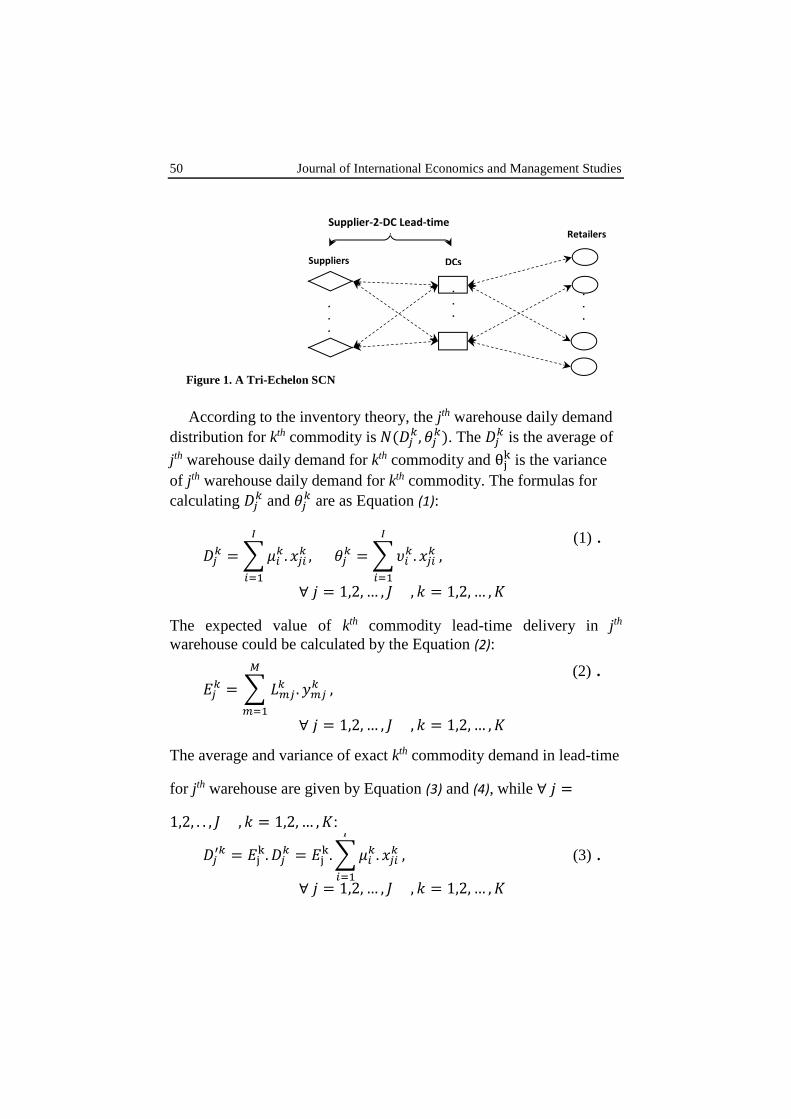
As shown in Figure 1 the assumed tri-echelon SCN for this paper
consists of suppliers to the left, distribution centers (DCs) in the
middle, and retailer nodes to the right. It has supposed that this
proposed SC Network:
i. Has an integrated structure consisting both potential supplier and
potential DCs designed to procure retailer demands for multitude
commodities.
ii. Has predefined numbers of suppliers and DCs with known
capacities.
iii. The number of its retailers and their demands distribution are
known.
iv. It operates in an uncertain circumstance, i.e. its main interior
parameters as demands, lead-time, procure and transportation
costs, and holding costs of inventory for commodities all are
supposed to be uniform random variables with known average
and variance (Table 1).
v. Its DCs and suppliers all are supposed to be potentially
operational at the beginning of the constructing network.
vi. Its suppliers and DCs do their procuring, shipment, and holding
duties perfect.
vii. Any retailer receives its demand for a specific merchandize only
from one DC.
viii. Shortage cannot happen at retailer nodes in any form.
ix. More than one supplier can replete the demand of a specific DC.
x. More than one DC can replete the demand of each retailer.
50 Journal of International Economics and Management Studies
According to the inventory theory, the jth warehouse daily demand
distribution for kth commodity is 𝑁(𝐷𝑗𝑘, 𝜃𝑗
𝑘). The 𝐷𝑗𝑘 is the average of
jth warehouse daily demand for kth commodity and θjk is the variance
of jth warehouse daily demand for kth commodity. The formulas for
calculating 𝐷𝑗𝑘 and 𝜃𝑗
𝑘 are as Equation (1):
𝐷𝑗𝑘 =∑𝜇𝑖
𝑘. 𝑥𝑗𝑖𝑘
𝐼
𝑖=1
, 𝜃𝑗𝑘 =∑𝜐𝑖
𝑘. 𝑥𝑗𝑖𝑘
𝐼
𝑖=1
,
∀ 𝑗 = 1,2, … , 𝐽 , 𝑘 = 1,2, … , 𝐾
(1) .
The expected value of kth commodity lead-time delivery in jth
warehouse could be calculated by the Equation (2):
𝐸𝑗𝑘 = ∑ 𝐿𝑚𝑗
𝑘 . 𝑦𝑚𝑗𝑘
𝑀
𝑚=1
,
∀ 𝑗 = 1,2, … , 𝐽 , 𝑘 = 1,2, … , 𝐾
(2) .
The average and variance of exact kth commodity demand in lead-time
for jth warehouse are given by Equation (3) and (4), while ∀ 𝑗 =
1,2, . . , 𝐽 , 𝑘 = 1,2, … , 𝐾:
𝐷𝑗′𝑘 = 𝐸j
k. 𝐷𝑗𝑘 = 𝐸j
k.∑𝜇𝑖𝑘. 𝑥𝑗𝑖
𝑘
𝐼
𝑖=1
,
∀ 𝑗 = 1,2, … , 𝐽 , 𝑘 = 1,2, … , 𝐾
(3) .
.
.
.
.
.
.
Supplier-2-DC Lead-time
Suppliers DCs
Retailers
.
.
.
Figure 1. A Tri-Echelon SCN
Optimizing Bi-Objective Multi-Commodity… 51
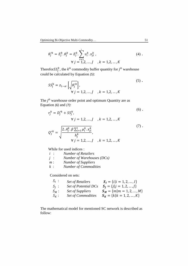
𝜃𝑗′𝑘 = 𝐸𝑗
𝑘. 𝜃𝑗𝑘 = 𝐸𝑗
𝑘.∑𝜐𝑖𝑘. 𝑥𝑗𝑖
𝑘
𝐼
𝑖=1
,
∀ 𝑗 = 1,2, … , 𝐽 , 𝑘 = 1,2, … , 𝐾
(4) .
Therefor𝑆𝑆𝑗𝑘, the kth commodity buffer quantity for jth warehouse
could be calculated by Equation (5):
𝑆𝑆jk = 𝑧1−𝛼. [√𝜃𝑗
′𝑘] ,
∀ 𝑗 = 1,2, … , 𝐽 , 𝑘 = 1,2, … , 𝐾
(5) .
The jth warehouse order point and optimum Quantity are as
Equation (6) and (7):
𝑟𝑗𝑘 = 𝐷𝑗
′𝑘 + 𝑆𝑆𝑗𝑘,
∀ 𝑗 = 1,2, … , 𝐽 , 𝑘 = 1,2, … , 𝐾
(6) .
𝑄𝑗∗𝑘 = √
2. 𝐴𝑗𝑘 . 𝛽 ∑ 𝜇𝑖
𝑘. 𝑥𝑗𝑖𝑘𝐼
𝑖=1
ℎ𝑗𝑘 ,
∀ 𝑗 = 1,2, … , 𝐽 , 𝑘 = 1,2, … , 𝐾
(7) .
While for used indices :
i : Number of Retailers
j : Number of Warehouses (DCs)
m : Number of Suppliers
k : Number of Commodities
Considered on sets:
𝑆𝐼 : Set of Retailers 𝑺𝑰 = {𝑖|𝑖 = 1, 2, … , 𝐼} 𝑆𝐽 : Set of Potential DCs 𝑺𝑱 = {𝑗|𝑗 = 1, 2, … , 𝐽}
𝑆𝑀 : Set of Suppliers 𝑺𝑴 = {𝑚|𝑚 = 1, 2, … ,𝑀} 𝑆𝐾 : Set of Commodities 𝑺𝑲 = {𝑘|𝑘 = 1, 2, … , 𝐾}
The mathematical model for mentioned SC network is described as
follow:
52 Journal of International Economics and Management Studies
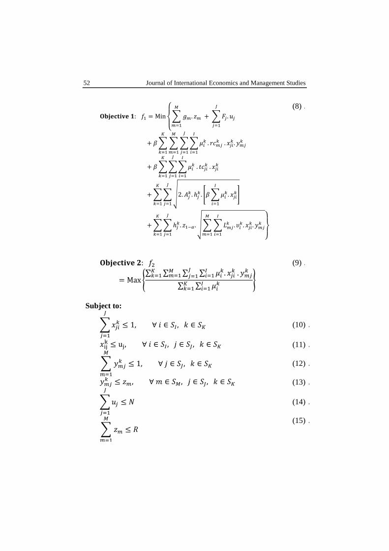
𝐎𝐛𝐣𝐞𝐜𝐭𝐢𝐯𝐞 𝟏: 𝑓1 = Min
{
∑ 𝑔𝑚. 𝑧𝑚
𝑀
𝑚=1
+ ∑𝐹𝑗. 𝑢𝑗
𝐽
𝑗=1
+ 𝛽∑∑∑∑𝜇𝑖𝑘
𝐼
𝑖=1
. 𝑟𝑐𝑚𝑗𝑘 . 𝑥𝑗𝑖
𝑘 . 𝑦𝑚𝑗𝑘
𝐽
𝑗=1
𝑀
𝑚=1
𝐾
𝑘=1
+ 𝛽∑∑∑𝜇𝑖𝑘 . 𝑡𝑐𝑗𝑖
𝑘 . 𝑥𝑗𝑖𝑘
𝐼
𝑖=1
𝐽
𝑗=1
𝐾
𝑘=1
+∑∑√2. 𝐴𝑗𝑘 . ℎ𝑗
𝑘 . [𝛽∑𝜇𝑖𝑘 . 𝑥𝑗𝑖
𝑘
𝐼
𝑖=1
]
𝐽
𝑗=1
𝐾
𝑘=1
+∑∑ℎ𝑗𝑘 . 𝑧1−𝛼 . √∑∑𝐿𝑚𝑗
𝑘 . 𝜐𝑖𝑘 . 𝑥𝑗𝑖
𝑘. 𝑦𝑚𝑗𝑘
𝐼
𝑖=1
𝑀
𝑚=1
𝐽
𝑗=1
𝐾
𝑘=1}
(8) .
𝐎𝐛𝐣𝐞𝐜𝐭𝐢𝐯𝐞 𝟐: 𝑓2
= Max {∑ ∑ ∑ ∑ 𝜇𝑖
𝑘. 𝑥𝑗𝑖𝑘 . 𝑦𝑚𝑗
𝑘𝐼𝑖=1
𝐽𝑗=1
𝑀𝑚=1
𝐾𝑘=1
∑ ∑ 𝜇𝑖𝑘𝐼
𝑖=1𝐾𝑘=1
}
(9) .
Subject to:
∑𝑥𝑗𝑖𝑘
𝐽
𝑗=1
≤ 1, ∀ 𝑖 ∈ 𝑆𝐼 , 𝑘 ∈ 𝑆𝐾 (10) .
𝑥ijk ≤ uj, ∀ 𝑖 ∈ 𝑆𝐼 , 𝑗 ∈ 𝑆𝐽, 𝑘 ∈ 𝑆𝐾 (11) .
∑ 𝑦𝑚𝑗𝑘
𝑀
𝑚=1
≤ 1, ∀ 𝑗 ∈ 𝑆𝐽, 𝑘 ∈ 𝑆𝐾 (12) .
𝑦𝑚𝑗𝑘 ≤ 𝑧𝑚, ∀ 𝑚 ∈ 𝑆𝑀, 𝑗 ∈ 𝑆𝐽, 𝑘 ∈ 𝑆𝐾 (13) .
∑𝑢𝑗 ≤ 𝑁
𝐽
𝑗=1
(14) .
∑ 𝑧𝑚
𝑀
𝑚=1
≤ 𝑅
(15) .
Optimizing Bi-Objective Multi-Commodity… 53
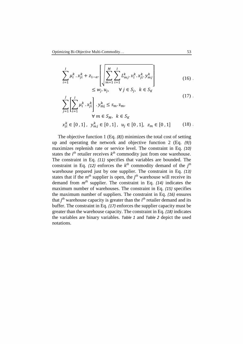
∑𝜇𝑖𝑘
𝐼
𝑖=1
. 𝑥𝑗𝑖𝑘 + 𝑧1−𝛼.
[ √∑∑𝐿𝑚𝑗
𝑘 . 𝜐𝑖𝑘. 𝑥𝑗𝑖
𝑘 . 𝑦𝑚𝑗𝑘
𝐼
𝑖=1
𝑀
𝑚=1]
≤ 𝑤𝑗. 𝑢𝑗 , ∀ 𝑗 ∈ 𝑆𝐽, 𝑘 ∈ 𝑆𝐾
(16) .
∑[∑𝜇𝑖𝑘
𝐼
𝑖=1
. 𝑥𝑗𝑖𝑘]
𝐽
𝑗=1
. 𝑦mjk ≤ 𝑠m. zm,
∀ 𝑚 ∈ 𝑆𝑀, 𝑘 ∈ 𝑆𝐾
(17) .
𝑥𝑗𝑖𝑘 ∈ [0 , 1] , 𝑦𝑚𝑗
𝑘 ∈ [0 , 1] , 𝑢𝑗 ∈ [0 , 1], 𝑧𝑚 ∈ [0 , 1] (18) .
The objective function 1 (Eq. (8)) minimizes the total cost of setting
up and operating the network and objective function 2 (Eq. (9))
maximizes replenish rate or service level. The constraint in Eq. (10)
states the ith retailer receives kth commodity just from one warehouse.
The constraint in Eq. (11) specifies that variables are bounded. The
constraint in Eq. (12) enforces the kth commodity demand of the jth
warehouse prepared just by one supplier. The constraint in Eq. (13)
states that if the mth supplier is open, the jth warehouse will receive its
demand from mth supplier. The constraint in Eq. (14) indicates the
maximum number of warehouses. The constraint in Eq. (15) specifies
the maximum number of suppliers. The constraint in Eq. (16) ensures
that jth warehouse capacity is greater than the ith retailer demand and its
buffer. The constraint in Eq. (17) enforces the supplier capacity must be
greater than the warehouse capacity. The constraint in Eq. (18) indicates
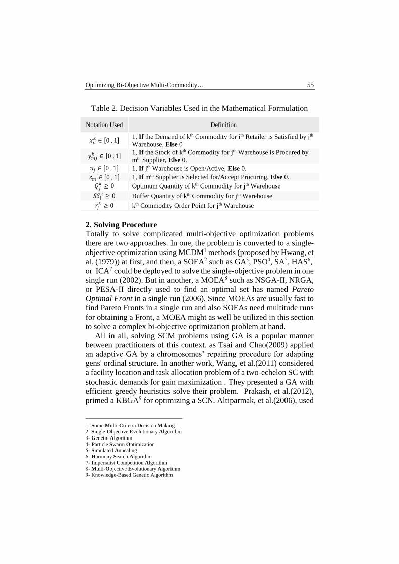
the variables are binary variables. Table 1 and Table 2 depict the used
notations.
54 Journal of International Economics and Management Studies
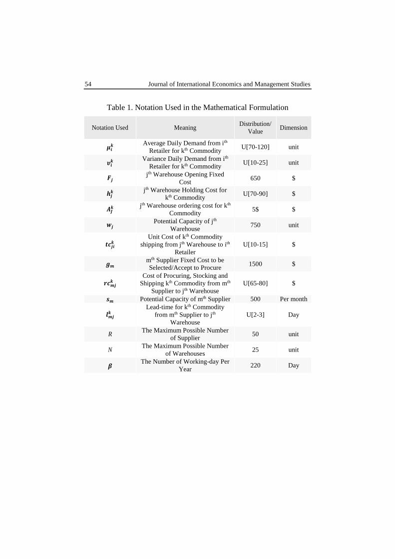
Table 1. Notation Used in the Mathematical Formulation
Notation Used Meaning Distribution/
Value Dimension
𝝁𝒊𝒌
Average Daily Demand from ith
Retailer for kth Commodity U[70-120] unit
𝝊𝒊𝒌
Variance Daily Demand from ith
Retailer for kth Commodity U[10-25] unit
𝑭𝒋 jth Warehouse Opening Fixed
Cost 650 $
𝒉𝒋𝒌
jth Warehouse Holding Cost for
kth Commodity U[70-90] $
𝑨𝑱𝒌
jth Warehouse ordering cost for kth
Commodity 5$ $
𝒘𝒋 Potential Capacity of jth
Warehouse 750 unit
𝒕𝒄𝒋𝒊𝒌
Unit Cost of kth Commodity
shipping from jth Warehouse to ith
Retailer
U[10-15] $
𝒈𝒎 mth Supplier Fixed Cost to be
Selected/Accept to Procure 1500 $
𝒓𝒄𝒎𝒋𝒌
Cost of Procuring, Stocking and
Shipping kth Commodity from mth
Supplier to jth Warehouse
U[65-80] $
𝒔𝒎 Potential Capacity of mth Supplier 500 Per month
𝒍𝒎𝒋𝒌
Lead-time for kth Commodity
from mth Supplier to jth
Warehouse
U[2-3] Day
R The Maximum Possible Number
of Supplier 50 unit
N The Maximum Possible Number
of Warehouses 25 unit
𝜷 The Number of Working-day Per
Year 220 Day
Optimizing Bi-Objective Multi-Commodity… 55
Table 2. Decision Variables Used in the Mathematical Formulation
Notation Used Definition
𝑥𝑗𝑖𝑘 ∈ [0 , 1]
1, If the Demand of kth Commodity for ith Retailer is Satisfied by jth
Warehouse, Else 0
𝑦𝑚𝑗𝑘 ∈ [0 , 1]
1, If the Stock of kth Commodity for jth Warehouse is Procured by
mth Supplier, Else 0.
𝑢𝑗 ∈ [0 , 1] 1, If jth Warehouse is Open/Active, Else 0.
𝑧𝑚 ∈ [0 , 1] 1, If mth Supplier is Selected for/Accept Procuring, Else 0.
𝑄𝑗𝑘 ≥ 0 Optimum Quantity of kth Commodity for jth Warehouse
𝑆𝑆jk ≥ 0 Buffer Quantity of kth Commodity for jth Warehouse
𝑟𝑗𝑘 ≥ 0 kth Commodity Order Point for jth Warehouse
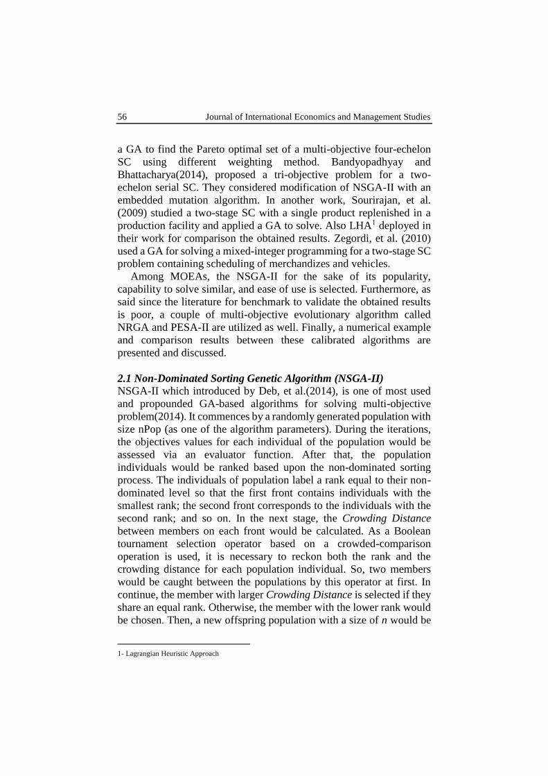
2. Solving Procedure
Totally to solve complicated multi-objective optimization problems
there are two approaches. In one, the problem is converted to a single-
objective optimization using MCDM1 methods (proposed by Hwang, et
al. (1979)) at first, and then, a SOEA2 such as GA3, PSO4, SA5, HAS6,
or ICA7 could be deployed to solve the single-objective problem in one
single run (2002). But in another, a MOEA8 such as NSGA-II, NRGA,
or PESA-II directly used to find an optimal set has named Pareto
Optimal Front in a single run (2006). Since MOEAs are usually fast to
find Pareto Fronts in a single run and also SOEAs need multitude runs
for obtaining a Front, a MOEA might as well be utilized in this section
to solve a complex bi-objective optimization problem at hand.
All in all, solving SCM problems using GA is a popular manner
between practitioners of this context. as Tsai and Chao(2009) applied
an adaptive GA by a chromosomes’ repairing procedure for adapting
gens' ordinal structure. In another work, Wang, et al.(2011) considered
a facility location and task allocation problem of a two-echelon SC with
stochastic demands for gain maximization . They presented a GA with
efficient greedy heuristics solve their problem. Prakash, et al.(2012),
primed a KBGA9 for optimizing a SCN. Altiparmak, et al.(2006), used
1- Some Multi-Criteria Decision Making 2- Single-Objective Evolutionary Algorithm
3- Genetic Algorithm
4- Particle Swarm Optimization 5- Simulated Annealing
6- Harmony Search Algorithm
7- Imperialist Competition Algorithm 8- Multi-Objective Evolutionary Algorithm
9- Knowledge-Based Genetic Algorithm
56 Journal of International Economics and Management Studies
a GA to find the Pareto optimal set of a multi-objective four-echelon
SC using different weighting method. Bandyopadhyay and
Bhattacharya(2014), proposed a tri-objective problem for a two-
echelon serial SC. They considered modification of NSGA-II with an
embedded mutation algorithm. In another work, Sourirajan, et al.
(2009) studied a two-stage SC with a single product replenished in a
production facility and applied a GA to solve. Also LHA1 deployed in
their work for comparison the obtained results. Zegordi, et al. (2010)
used a GA for solving a mixed-integer programming for a two-stage SC
problem containing scheduling of merchandizes and vehicles.
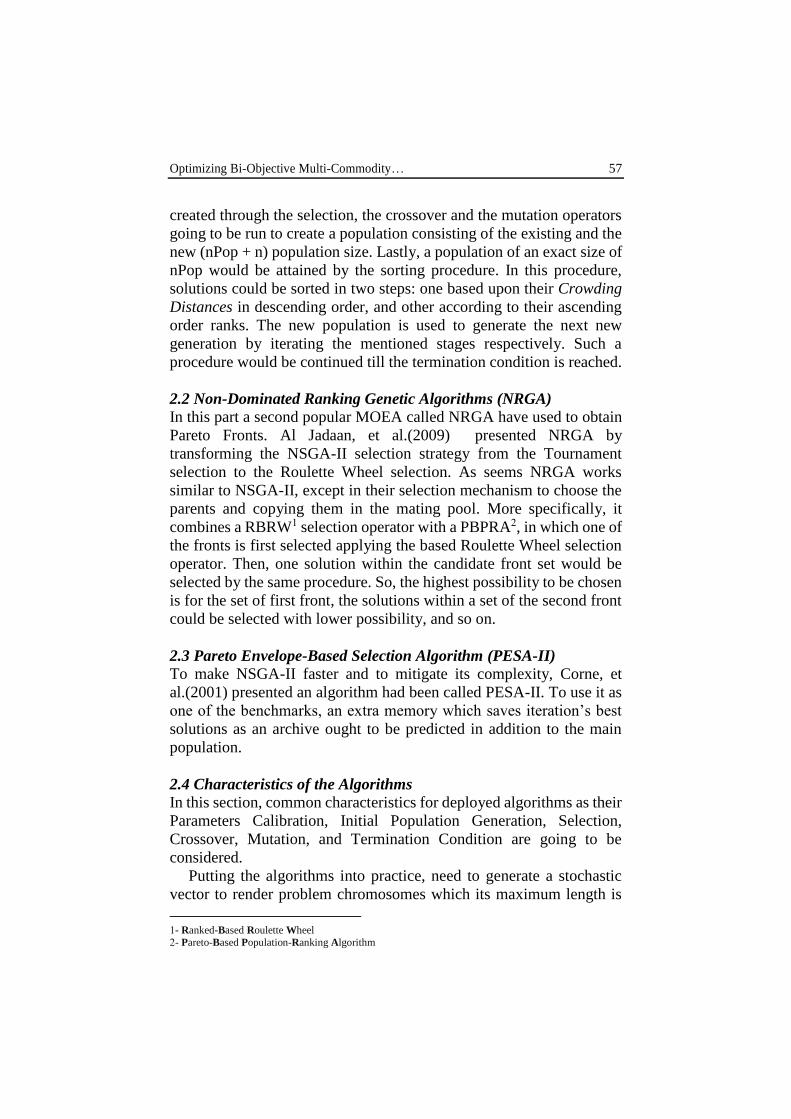
Among MOEAs, the NSGA-II for the sake of its popularity,
capability to solve similar, and ease of use is selected. Furthermore, as
said since the literature for benchmark to validate the obtained results
is poor, a couple of multi-objective evolutionary algorithm called
NRGA and PESA-II are utilized as well. Finally, a numerical example
and comparison results between these calibrated algorithms are
presented and discussed.
2.1 Non-Dominated Sorting Genetic Algorithm (NSGA-II)
NSGA-II which introduced by Deb, et al.(2014), is one of most used
and propounded GA-based algorithms for solving multi-objective
problem(2014). It commences by a randomly generated population with
size nPop (as one of the algorithm parameters). During the iterations,
the objectives values for each individual of the population would be
assessed via an evaluator function. After that, the population
individuals would be ranked based upon the non-dominated sorting
process. The individuals of population label a rank equal to their non-
dominated level so that the first front contains individuals with the
smallest rank; the second front corresponds to the individuals with the
second rank; and so on. In the next stage, the Crowding Distance
between members on each front would be calculated. As a Boolean
tournament selection operator based on a crowded-comparison
operation is used, it is necessary to reckon both the rank and the
crowding distance for each population individual. So, two members
would be caught between the populations by this operator at first. In
continue, the member with larger Crowding Distance is selected if they
share an equal rank. Otherwise, the member with the lower rank would
be chosen. Then, a new offspring population with a size of n would be
1- Lagrangian Heuristic Approach
Optimizing Bi-Objective Multi-Commodity… 57
created through the selection, the crossover and the mutation operators
going to be run to create a population consisting of the existing and the
new (nPop + n) population size. Lastly, a population of an exact size of
nPop would be attained by the sorting procedure. In this procedure,
solutions could be sorted in two steps: one based upon their Crowding
Distances in descending order, and other according to their ascending
order ranks. The new population is used to generate the next new
generation by iterating the mentioned stages respectively. Such a
procedure would be continued till the termination condition is reached.
2.2 Non-Dominated Ranking Genetic Algorithms (NRGA)
In this part a second popular MOEA called NRGA have used to obtain
Pareto Fronts. Al Jadaan, et al.(2009) presented NRGA by
transforming the NSGA-II selection strategy from the Tournament
selection to the Roulette Wheel selection. As seems NRGA works
similar to NSGA-II, except in their selection mechanism to choose the
parents and copying them in the mating pool. More specifically, it
combines a RBRW1 selection operator with a PBPRA2, in which one of
the fronts is first selected applying the based Roulette Wheel selection
operator. Then, one solution within the candidate front set would be
selected by the same procedure. So, the highest possibility to be chosen
is for the set of first front, the solutions within a set of the second front
could be selected with lower possibility, and so on.
2.3 Pareto Envelope-Based Selection Algorithm (PESA-II)
To make NSGA-II faster and to mitigate its complexity, Corne, et
al.(2001) presented an algorithm had been called PESA-II. To use it as
one of the benchmarks, an extra memory which saves iteration’s best
solutions as an archive ought to be predicted in addition to the main
population.
2.4 Characteristics of the Algorithms
In this section, common characteristics for deployed algorithms as their
Parameters Calibration, Initial Population Generation, Selection,
Crossover, Mutation, and Termination Condition are going to be
considered.
Putting the algorithms into practice, need to generate a stochastic
vector to render problem chromosomes which its maximum length is
1- Ranked-Based Roulette Wheel
2- Pareto-Based Population-Ranking Algorithm

58 Journal of International Economics and Management Studies
equal to problem variables. These stochastic numbers have four
portions. 1st and 2nd are Boolean variable each of which defines active
DCs and Suppliers between existing ones. 3rd and 4th parts would be
generated by preliminary parts (1st & 2nd) and defines X & Y variables.
Note that each X & Y are three dimensional Boolean variables. (X
dimensions = number of DCs × number of retailers × number of
commodities). So it's necessary to generate a stochastic number series
with size of "number of retailers × number of commodities " from
active DCs set (exposing X) and also a stochastic number series with
size of " number of active DCs × number of commodities " from active
suppliers set (exposing Y), to represent them by vector.
2.4.1 Representation of the Chromosomes
In order to embody each solution as a chromosome, one binary vector
is used for integer-valued variables. Let's suppose that the number of
potential DCs, the number of potential suppliers, the number of
retailers, and the number of commodities are 3, 4, 2, & 2 respectively.
Figure 2 presents a generated chromosome with mentioned method.
Figure 2. A Case in Chromosome Representation
As the Figure 2 shows, the generated chromosome is containing 4
parts. The DCs 1 & 3 both are active DCs and the DC 2 is null. Second
part also refers that suppliers 1, 2, & 4 are a set of active suppliers. 3rd
portion of the chromosome contain a stochastic chain between active
DCs (1 & 3) that its length is equal to "number of retailers × number of
commodities". This section divided into subsets (number of retailers)
per se, and length of each one is equal to the number of commodities.
This section tells that 1st retailer delivers 1st commodity from 3rd DC
and 2nd commodity from 1st DC. Also 2nd retailer delivers both 1st and
2nd commodities from 1st DC. Last portion of chromosome have
stochastic chain between active suppliers (i.e. 1, 2, & 4) that its length
is equal to "active DCs × number of commodities". This section also
divided into subsets (coincide with number of DCs) that the length of
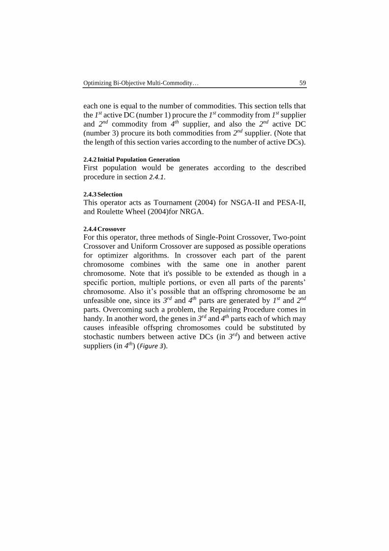
Optimizing Bi-Objective Multi-Commodity… 59
each one is equal to the number of commodities. This section tells that
the 1st active DC (number 1) procure the 1st commodity from 1st supplier
and 2nd commodity from 4th supplier, and also the 2nd active DC
(number 3) procure its both commodities from 2nd supplier. (Note that
the length of this section varies according to the number of active DCs).
2.4.2 Initial Population Generation
First population would be generates according to the described
procedure in section 2.4.1.
2.4.3 Selection
This operator acts as Tournament (2004) for NSGA-II and PESA-II,
and Roulette Wheel (2004)for NRGA.
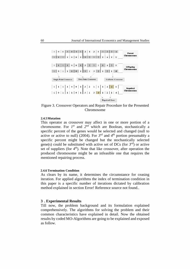
2.4.4 Crossover
For this operator, three methods of Single-Point Crossover, Two-point
Crossover and Uniform Crossover are supposed as possible operations
for optimizer algorithms. In crossover each part of the parent
chromosome combines with the same one in another parent
chromosome. Note that it's possible to be extended as though in a
specific portion, multiple portions, or even all parts of the parents’
chromosome. Also it’s possible that an offspring chromosome be an
unfeasible one, since its 3rd and 4th parts are generated by 1st and 2nd
parts. Overcoming such a problem, the Repairing Procedure comes in
handy. In another word, the genes in 3rd and 4th parts each of which may
causes infeasible offspring chromosomes could be substituted by
stochastic numbers between active DCs (in 3rd) and between active
suppliers (in 4th) (Figure 3).
60 Journal of International Economics and Management Studies
Figure 3. Crossover Operators and Repair Procedure for the Presented
Chromosome
2.4.5 Mutation
This operator as crossover may affect in one or more portion of a
chromosome. For 1st and 2nd which are Boolean, stochastically a
specific percent of the genes would be selected and changed (null to
active or active to null) (2004). For 3rd and 4th portion presumably a
specific percent might be changed but the stochastically selected
gene(s) could be substituted with active set of DCs (for 3rd) or active
set of suppliers (for 4th). Note that like crossover, after operation the
produced chromosome might be an infeasible one that requires the
mentioned repairing process.
2.4.6 Termination Condition
As clears by its name, it determines the circumstance for ceasing
iteration. For applied algorithms the index of termination condition in
this paper is a specific number of iterations dictated by calibration
method explained in section Error! Reference source not found..
3 . Experimental Results
Till now, the problem background and its formulation explained
comprehensively. The algorithms for solving the problem and their
common characteristics have explained in detail. Now the obtained
results by coded MO-Algorithms are going to be explained and exposed
as follow.

Optimizing Bi-Objective Multi-Commodity… 61
3.1 NSGA-II
The produced results by this algorithm reported in Figure 4.
Figure 4. Generated Pareto Front by NSGA-II
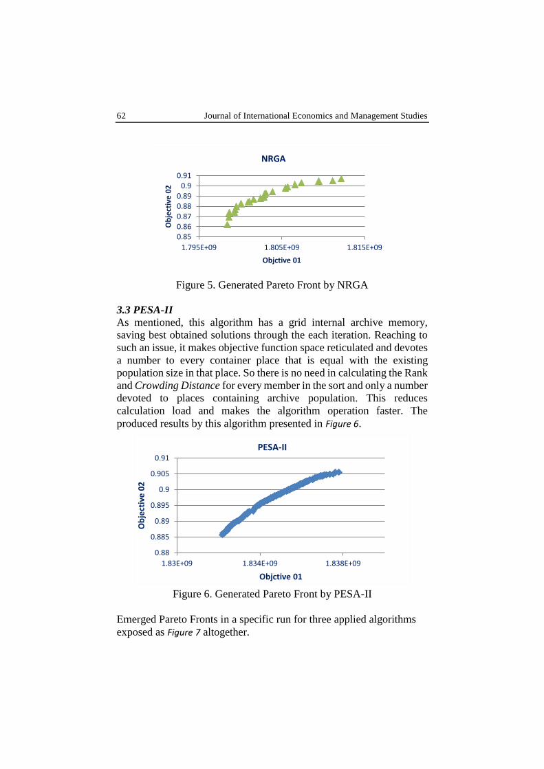
3.2 NRGA
As pronounced, the different between this algorithm and NSGAII is in
their member selection. This algorithm uses Roulette Wheel based upon
the sorting for parent selection, which is a modified usage of generic
Roulette Wheel. According to this modification, the possibility of
selection a member like i from population is equal to Pi and could be
calculated by Formula (19).
𝑷𝒊 =2 ∗ 𝑅𝑎𝑛𝑘𝑖
𝑛𝑃𝑜𝑝 ∗ (𝑛𝑃𝑜𝑝 + 1)
(19) .
Note that the N is population size, and 𝑅𝑎𝑛𝑘𝑖 is ith member rank in
population. The results of this algorithm exposed in Figure 5.
0.89
0.895
0.9
0.905
0.91
0.915
0.92
0.925
1.805E+09 1.81E+09 1.815E+09 1.82E+09
Ob
ject
ive
02
Objctive 01
NSGA-II
62 Journal of International Economics and Management Studies
Figure 5. Generated Pareto Front by NRGA
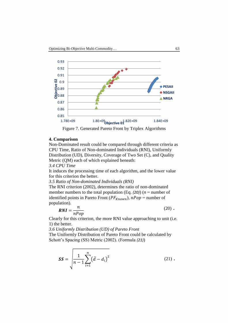
3.3 PESA-II
As mentioned, this algorithm has a grid internal archive memory,
saving best obtained solutions through the each iteration. Reaching to
such an issue, it makes objective function space reticulated and devotes
a number to every container place that is equal with the existing
population size in that place. So there is no need in calculating the Rank
and Crowding Distance for every member in the sort and only a number
devoted to places containing archive population. This reduces
calculation load and makes the algorithm operation faster. The
produced results by this algorithm presented in Figure 6.
Figure 6. Generated Pareto Front by PESA-II
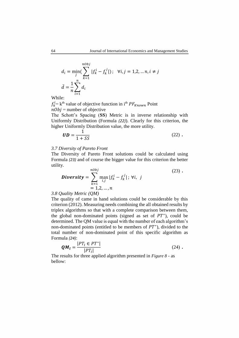
Emerged Pareto Fronts in a specific run for three applied algorithms
exposed as Figure 7 altogether.
0.850.860.870.880.89
0.90.91
1.795E+09 1.805E+09 1.815E+09
Ob
ject
ive
02
Objctive 01
NRGA
0.88
0.885
0.89
0.895
0.9
0.905
0.91
1.83E+09 1.834E+09 1.838E+09
Ob
ject
ive
02
Objctive 01
PESA-II
Optimizing Bi-Objective Multi-Commodity… 63
Figure 7. Generated Pareto Front by Triplex Algorithms
4. Comparison
Non-Dominated result could be compared through different criteria as
CPU Time, Ratio of Non-dominated Individuals (RNI), Uniformly
Distribution (UD), Diversity, Coverage of Two Set (C), and Quality
Metric (QM) each of which explained beneath:
3.4 CPU Time
It induces the processing time of each algorithm, and the lower value
for this criterion the better.
3.5 Ratio of Non-dominated Individuals (RNI)
The RNI criterion (2002), determines the ratio of non-dominated
member numbers to the total population (Eq. (20)) (n = number of
identified points in Pareto Front (𝑃𝐹𝐾𝑛𝑜𝑤𝑛), 𝑛𝑃𝑜𝑝 = number of
population).
𝑹𝑵𝑰 =𝑛
𝑛𝑃𝑜𝑝 (20) .
Clearly for this criterion, the more RNI value approaching to unit (i.e.
1) the better.
3.6 Uniformly Distribution (UD) of Pareto Front
The Uniformly Distribution of Pareto Front could be calculated by
Schott’s Spacing (SS) Metric (2002). (Formula (21))
𝑺𝑺 = √1
𝑛 − 1∑(�̅� − 𝑑𝑖)
2𝑛
𝑖=1
(21) .
0.85
0.86
0.87
0.88
0.89
0.9
0.91
0.92
0.93
1.78E+09 1.8E+09 1.82E+09 1.84E+09
Ob
ject
ive
02
Objective 01
PESAII
NSGAII
NRGA
64 Journal of International Economics and Management Studies
𝑑𝑖 = min𝑗(∑ |𝑓𝑘
𝑖 − 𝑓𝑘𝑗|
𝑛𝑂𝑏𝑗
𝑘=1
) ; ∀𝑖, 𝑗 = 1,2, …𝑛, 𝑖 ≠ 𝑗
�̅� =1
𝑛∑𝑑𝑖
𝑛
𝑖=1
While:
𝑓𝑘𝑖= kth value of objective function in ith 𝑃𝐹𝐾𝑛𝑜𝑤𝑛 Point
𝑛𝑂𝑏𝑗 = number of objective
The Schott’s Spacing (SS) Metric is in inverse relationship with
Uniformly Distribution (Formula (22)). Clearly for this criterion, the
higher Uniformly Distribution value, the more utility.
𝑼𝑫 =1
1 + 𝑆𝑆 (22) .
3.7 Diversity of Pareto Front
The Diversity of Pareto Front solutions could be calculated using
Formula (23) and of course the bigger value for this criterion the better
utility.
𝑫𝒊𝒗𝒆𝒓𝒔𝒊𝒕𝒚 = ∑ max𝑖,𝑗
|𝑓𝑘𝑖 − 𝑓𝑘
𝑗|
𝑛𝑂𝑏𝑗
𝑘=1
; ∀𝑖, 𝑗
= 1,2, … , 𝑛
(23) .
3.8 Quality Metric (QM) The quality of came in hand solutions could be considerable by this
criterion (2012). Measuring needs combining the all obtained results by
triplex algorithms so that with a complete comparison between them,
the global non-dominated points (signed as set of 𝑃𝑇∗), could be
determined. The QM value is equal with the number of each algorithm’s
non-dominated points (entitled to be members of 𝑃𝑇∗), divided to the
total number of non-dominated point of this specific algorithm as
Formula (24):
𝑸𝑴𝒍 =|𝑃𝑇𝑙 ∈ 𝑃𝑇
∗|
|𝑃𝑇𝑙| (24) .
The results for three applied algorithm presented in Figure 8 - as
bellow:

Optimizing Bi-Objective Multi-Commodity… 65
Figure 8. Line Plot and Box Plot for CPU Time
Figure 9. Line Plot and Box Plot for RNI
66 Journal of International Economics and Management Studies
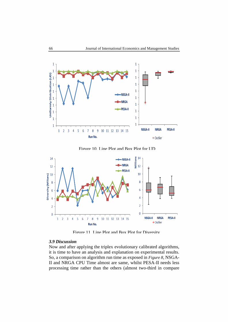
3.9 Discussion
Now and after applying the triplex evolutionary calibrated algorithms,
it is time to have an analysis and explanation on experimental results.
So, a comparison on algorithm run time as exposed in Figure 8, NSGA-
II and NRGA CPU Time almost are same, whilst PESA-II needs less
processing time rather than the others (almost two-third in compare
Figure 10. Line Plot and Box Plot for UD
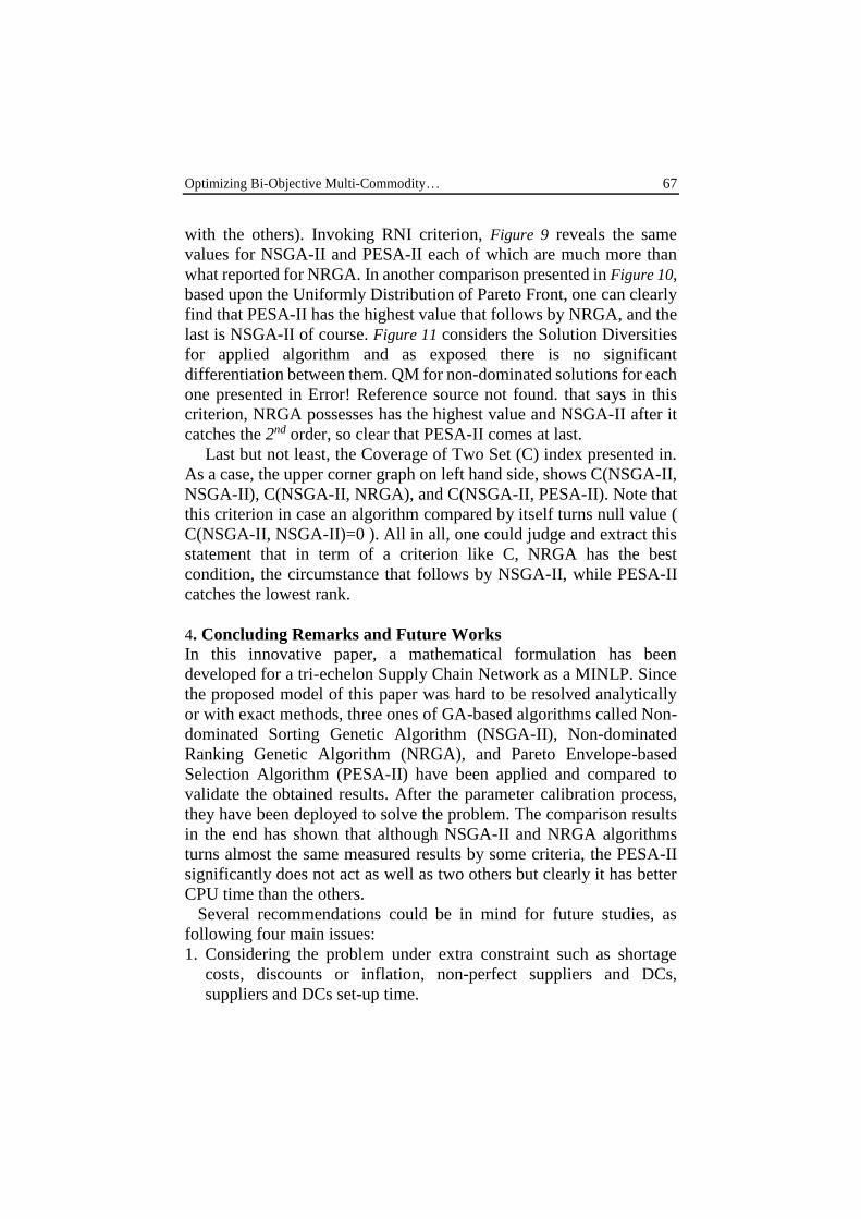
Figure 11. Line Plot and Box Plot for Diversity
Optimizing Bi-Objective Multi-Commodity… 67
with the others). Invoking RNI criterion, Figure 9 reveals the same
values for NSGA-II and PESA-II each of which are much more than
what reported for NRGA. In another comparison presented in Figure 10,
based upon the Uniformly Distribution of Pareto Front, one can clearly
find that PESA-II has the highest value that follows by NRGA, and the
last is NSGA-II of course. Figure 11 considers the Solution Diversities
for applied algorithm and as exposed there is no significant
differentiation between them. QM for non-dominated solutions for each
one presented in Error! Reference source not found. that says in this
criterion, NRGA possesses has the highest value and NSGA-II after it
catches the 2nd order, so clear that PESA-II comes at last.
Last but not least, the Coverage of Two Set (C) index presented in.
As a case, the upper corner graph on left hand side, shows C(NSGA-II,
NSGA-II), C(NSGA-II, NRGA), and C(NSGA-II, PESA-II). Note that
this criterion in case an algorithm compared by itself turns null value (
C(NSGA-II, NSGA-II)=0 ). All in all, one could judge and extract this
statement that in term of a criterion like C, NRGA has the best
condition, the circumstance that follows by NSGA-II, while PESA-II
catches the lowest rank.
4. Concluding Remarks and Future Works In this innovative paper, a mathematical formulation has been
developed for a tri-echelon Supply Chain Network as a MINLP. Since
the proposed model of this paper was hard to be resolved analytically
or with exact methods, three ones of GA-based algorithms called Non-
dominated Sorting Genetic Algorithm (NSGA-II), Non-dominated
Ranking Genetic Algorithm (NRGA), and Pareto Envelope-based
Selection Algorithm (PESA-II) have been applied and compared to
validate the obtained results. After the parameter calibration process,
they have been deployed to solve the problem. The comparison results
in the end has shown that although NSGA-II and NRGA algorithms
turns almost the same measured results by some criteria, the PESA-II
significantly does not act as well as two others but clearly it has better
CPU time than the others.
Several recommendations could be in mind for future studies, as
following four main issues:
1. Considering the problem under extra constraint such as shortage
costs, discounts or inflation, non-perfect suppliers and DCs,
suppliers and DCs set-up time.
68 Journal of International Economics and Management Studies
2. Utilizing other meta-heuristics such as MOGA, MOSA, MOPSO,
and MOHS to solve the problem and comparing their performances.
3. Using other GA operators for mutation and crossover.
4. Invoking queuing models as a hybridized portion for network and
also considering some of intake parameters as fuzzy numbers.
References
Rogers, D.S., Leuschner, R. (2004). Supply chain management:
retrospective and prospective, Journal of Marketing Theory and Practice,
pp. 60-65.
Handfield, R.B., Nichols, E. L.(1999). Introduction to supply chain
management vol. 183: prentice Hall Upper Saddle River.
Amiri, A. (2006). Designing a distribution network in a supply chain
system: Formulation and efficient solution procedure, European Journal of
Operational Research, vol. 171, pp. 567-576.
Gebennini, E., Gamberini, R., Manzini, R. (2009). An integrated
production–distribution model for the dynamic location and allocation
problem with safety stock optimization, International Journal of Production
Economics, vol. 122, pp. 286-304.
Mohammadi Bidhandi, H., Mohd Yusuff, R.(2011). Integrated supply chain
planning under uncertainty using an improved stochastic approach, Applied
Mathematical Modelling, vol. 35, pp. 2618-2630.
Snyder, L. V. (2006). Facility location under uncertainty: a review, IIE
Transactions, vol. 38, pp. 547-564.
Murthy, D. N. P., Solem, O. & Roren, T. (2004). Product warranty logistics:
Issues and challenges," European Journal of Operational Research, vol.
156, pp. 110-126.
Van Landeghem, H., Vanmaele, H.( 2002). Robust planning: a new
paradigm for demand chain planning. Journal of operations management,
vol. 20, pp. 769-783.
Jamshidi, R., Fatemi Ghomi S. M. T. & Karimi, B.( 2012). Multi-objective
green supply chain optimization with a new hybrid memetic algorithm using
the Taguchi method, Scientia Iranica, vol. 19, pp.1876-1886.
Moncayo-Martínez, L. A., Zhang, D. Z.( 2011). Multi-objective ant colony
optimisation: A meta-heuristic approach to supply chain design,
International Journal of Production Economics, vol. 131, pp. 407-420.
Cardona-Valdés, Y., Álvarez, A. & Pacheco, J. (2014). Metaheuristic
procedure for a bi-objective supply chain design problem with uncertainty,
Transportation Research Part B: Methodological, vol. 60, pp. 66-84.
Shankar, B. L., Basavarajappa, S., Chen, J. C. & Kadadevaramath, R. S.
(2013). Location and allocation decisions for multi-echelon supply chain
Optimizing Bi-Objective Multi-Commodity… 69
network–a multi-objective evolutionary approach, Expert Systems with
Applications, vol. 40, pp. 551-562.
Marufuzzaman, M., Eksioglu, S. D., Huang, Y.( 2014). Two-stage
stochastic programming supply chain model for biodiesel production via
wastewater treatment, Computers & Operations Research, vol. 49, pp. 1-
17.
Simchi-Levi, D., Kaminsky, P. & Simchi-Levi, E.( 2003). Designing and
Managing the Supply Chain: Concepts, Strategies, and Case Studies:
McGraw-Hill/Irwin.
Weber, A, Friedrich, C. J.( 1929). Alfred Weber's theory of the location of
industries,".
Hakimi, S. L.( 1964). Optimum locations of switching centers and the
absolute centers and medians of a graph, Operations research, vol. 12, pp.
450-459.
Daskin, M. (1997). Network and discrete location: models, algorithms and
applications. Journal of the Operational Research Society, vol. 48, pp. 763-
763.
Church, R. L., ReVelle, C. S.( 1976). Theoretical and Computational Links
between the p‐Median, Location Set‐covering, and the Maximal Covering
Location Problem. Geographical Analysis, vol. 8, pp. 406-415.
Warszawski, A. S.( 1973). Peer. Optimizing the location of facilities on a
building site. Journal of the Operational Research Society, vol. 24, pp. 35-
44.
Geoffrion, A. M., Graves, G. W. (1974). Multicommodity distribution
system design by Benders decomposition. Management science, vol. 20, pp.
822-844.
Mirchandani, P. B., Francis, R. L.( 1990). Discrete location theory.
Shen, Z.-J. M., Coullard, Daskin, M. S.(2003). A joint location-inventory
model. Transportation Science, vol. 37, pp. 40-55.
Sridharan, R.(1995). The capacitated plant location problem," European
Journal of Operational Research, vol. 87, pp. 203-213.
Ballou, R. H.(1968). Dynamic warehouse location analysis, Journal of
Marketing Research, pp. 271-276.
Scott, A. J.(1971). Dynamic location-allocation systems: some basic
planning strategies, Environment and Planning, vol. 3, pp. 73-82.
Wesolowsky, G. O., Truscott, W. G.(1975). The Multiperiod Location-
Allocation Problem with Relocation of Facilities, Management Science, vol.
22, pp. 57-65.
Erlenkotter, D.(1981). A comparative study of approaches to dynamic
location problems. European Journal of Operational Research, vol. 6, pp.
133-143.
70 Journal of International Economics and Management Studies
Azapagic, A., Clift, R.(1999). The application of life cycle assessment to
process optimisation. Computers & Chemical Engineering, vol. 23, pp.
1509-1526.
Chen, C.-L., Lee, W.-C.(2004). Multi-objective optimization of multi-
echelon supply chain networks with uncertain product demands and prices.
Computers & Chemical Engineering, vol. 28, pp. 1131-1144.
Zhou, Z., Cheng, S.& Hua, B.(2000). Supply chain optimization of
continuous process industries with sustainability considerations. Computers
& Chemical Engineering, vol. 24, pp. 1151-1158.
Sabri, E. H. & Beamon, B. M.(2000). A multi-objective approach to
simultaneous strategic and operational planning in supply chain design.
Omega, vol. 28, pp. 581-598.
Nozick, L. K., Turnquist, M. A.(2001). Inventory, transportation, service
quality and the location of distribution centers. European Journal of
Operational Research, vol. 129, pp. 362-371.
Chen, Z. L.( 2004). Integrated production and distribution operations:
Taxonomy, models, and review. INTERNATIONAL SERIES IN OPERATIONS
RESEARCH AND MANAGEMENT SCIENCE, pp. 711-746.
Kopanos, G. M., Laínez, J. M.& Puigjaner, L.(2009). An efficient mixed-
integer linear programming scheduling framework for addressing sequence-
dependent setup issues in batch plants. Industrial & Engineering Chemistry
Research, vol. 48, pp. 6346-6357.
Graves, S. C., Willems, S. P.(2005). Optimizing the Supply Chain
Configuration for New Products. Manage. Sci., vol. 51, pp. 1165-1180.
Goldberg, D. E.(1990). E.(1989). Genetic algorithms in search, optimization
and machine learning. Reading: Addison-Wesley.
Hwang, C.-L., Masud, A. S. M., Paidy, S. R. & Yoon, K. P.(1979). Multiple
objective decision making, methods and applications: a state-of-the-art
survey vol. 164: Springer Berlin.
Deb, K., Pratap, A., Agarwal, S. & Meyarivan, T.(2002). A fast and elitist
multiobjective genetic algorithm: NSGA-II. Evolutionary Computation,
IEEE Transactions on, vol. 6, pp. 182-197.
Al Jadaan, O.,. Rao, C. & Rajamani, L.(2006). Parametric study to enhance
genetic algorithm performance, using ranked based roulette wheel selection
method. in International Conference on Multidisciplinary Information
Sciences and Technology (InSciT2006), pp. 274-278.
Tsai, C.-F., Chao, K.-M.(2009). Chromosome refinement for optimising
multiple supply chains. Information Sciences, vol. 179, pp. 2403-2415.
Wang, K.-J., Makond, B. & Liu, S. Y.(2011). Location and allocation
decisions in a two-echelon supply chain with stochastic demand – A
genetic-algorithm based solution. Expert Systems with Applications, vol. 38,
pp. 6125-6131.
Optimizing Bi-Objective Multi-Commodity… 71
Prakash, A., Chan, F. T. S., Liao, H. & Deshmukh, S. G.(1012). Network
optimization in supply chain: A KBGA approach. Decision Support
Systems, vol. 52, pp. 528-538.
Altiparmak, F., Gen, M., Lin, L. & Paksoy, T.(2006). A genetic algorithm
approach for multi-objective optimization of supply chain networks.
Computers & Industrial Engineering, vol. 51, pp. 196-215.
Bandyopadhyay, S., Bhattacharya, R.(2014). Solving a tri-objective supply
chain problem with modified NSGA-II algorithm. Journal of
Manufacturing Systems, vol. 33, pp. 41-50.
Sourirajan, K., Ozsen, L. & Uzsoy, R.(2009). A genetic algorithm for a
single product network design model with lead time and safety stock
considerations. European Journal of Operational Research, vol. 197, pp.
599-608, 200.
Zegordi, S. H., Abadi, I. N. K. & B. Nia, M. A.(2010). A novel genetic
algorithm for solving production and transportation scheduling in a two-stage
supply chain. Computers & Industrial Engineering, vol. 58, pp. 373-381.
Deb, K., Agrawal, S., Pratap, A. & Meyarivan, T.(2000). A fast elitist non-
dominated sorting genetic algorithm for multi-objective optimization:
NSGA-II. Lecture notes in computer science, vol. 1917, pp. 849-858.
Alavidoost M. H., Nayeri, M. A.(2014). Proposition of a hybrid NSGA-II
algorithm with fuzzy objectives for bi-objective assembly line balancing
problem. in Tenth International Industrial Engineering Conference.
Al Jadaan, O., Rajamani, L. & Rao, C.(2009). Non-dominated ranked
genetic algorithm for solving constrained multi-objective optimization
problems. Journal of Theoretical & Applied Information Technology, vol.
5, pp. 640-651.
Corne, D. W., Jerram, N. R., Knowles, J. D. & Oates, M. J.(2001). PESA-
II: Region-based selection in evolutionary multiobjective optimization. in
Proceedings of the Genetic and Evolutionary Computation Conference.
Haupt, R. L., Haupt, S. E.(2004). Practical genetic algorithms: Wiley-
Interscience.
Tan, K. C., Lee, T. H. & Khor, E. F.(2002). Evolutionary algorithms for
multi-objective optimization: performance assessments and comparisons.
Artificial intelligence review, vol. 17, pp. 251-290.
Knowles, J. & Corne, D.(2002). On metrics for comparing nondominated
sets. in Evolutionary Computation, 2002. CEC'02. Proceedings of the 2002
Congress on, 2002, pp. 711-716.
Zitzler, E., Thiele, L.(1999). Multiobjective evolutionary algorithms: a
comparative case study and the strength Pareto approach. Evolutionary
Computation, IEEE Transactions on, vol. 3, pp. 257-271.
Rabiee, M., Zandieh, M. & Ramezani, P.(2012). Bi-objective partial flexible
job shop scheduling problem: NSGA-II, NRGA, MOGA and PAES
72 Journal of International Economics and Management Studies
approaches. International Journal of Production Research, vol. 50, pp.
7327-7342.
Ruiz, R., Maroto, C. & Alcaraz, J.(2006). Two new robust genetic algorithms
for the flowshop scheduling problem. Omega, vol. 34, pp. 461-476.
Montgomery, D. C.(2008). Design and analysis of experiments: John Wiley
& Sons.
Taguchi, G.(1986). Introduction to quality engineering: designing quality
into products and processes.
Alavidoost, M., Zarandi, M. F., Tarimoradi, M. & Nemati, Y.(2014).
Modified genetic algorithm for simple straight and U-shaped assembly line
balancing with fuzzy processing times. Journal of Intelligent
Manufacturing, pp. 1-24.
Naderi, B., Zandieh, M., Khaleghi Ghoshe Balagh, A. & Roshanaei,
V.(2009). An improved simulated annealing for hybrid flowshops with
sequence-dependent setup and transportation times to minimize total
completion time and total tardiness," Expert Systems with Applications, vol.
36, pp. 9625-9633.