ARTICLE IN PRESS

0378-4371/$ - se

doi:10.1016/j.ph

�CorrespondE-mail addr

Physica A 371 (2006) 627–632

www.elsevier.com/locate/physa

Optimized annealing of traveling salesman problem from thenth-nearest-neighbor distribution

Yong Chen�, Pan Zhang

Institute of Theoretical Physics, Lanzhou University, Lanzhou 730000, China

Received 21 January 2006; received in revised form 10 April 2006

Available online 17 May 2006

Abstract

We report a new statistical general property in traveling salesman problem, that the nth-nearest-neighbor distribution of

optimal tours verifies with very high accuracy an exponential decay as a function of the order of neighbor n. Defining the

energy function as deviation l from this exponential decay, which is different to the tour length d in normal annealing

processes, we propose a distinct highly optimized annealing scheme which is performed in l-space and d-space by turns.

The simulation results of some standard traveling salesman problems in TSPLIB95 are presented. It is shown that our

annealing recipe is superior to the canonical simulated annealing.

r 2006 Elsevier B.V. All rights reserved.

Keywords: Optimization; Simulated annealing; Traveling salesman problem (TSP); NP-complete

The traveling salesman problem (TSP) is stated for the shortest closed tour for a traveling salesman whomust visit each of N cities in turn [1–3]. The number of candidate sets is N!=2N. So it is very difficult to find anefficient algorithm for large N because it is bounded by a polynomial function with the problem size. Forexample, Padberg and Rinaldi obtained the optimal solution, i.e., the shortest path, for 532 US cities after 6 hof calculation with the use of the supercomputer Cyber 205 in 1987 [4]. And, the TSP is a classic, famous,nondeterministic polynomial problem (NP-complete) and a good testing ground for optimization methods.Because the exact solutions are almost impossible to obtain, the realistic and valuable aim is to seek for a near-optimal solution.

In recent several decades, TSP has attracted a lot of attention of many physicists, and lots of algorithmswith physical insight have been proposed. In 1982, Hopfield and Tank used neural networks to find theapproximate solution [5], and since then, simulated annealing (SA) [6,7,21], hierarchical construction [8], realspace renormalization [9–11], diffusion process [12], etc. have been introduced to challenge TSP.

Among these algorithms from statistical physics, the most general powerful solution is SA scheme [6,7]. Theclassical simulated annealing (CSA) was proposed by Kirkpatrick et al. [6], which extended the Metropolisprocedure for equilibrium Boltzmann–Gibbs statistics. Moreover, it was shown that the system will end in aglobal minimum if the temperature decreases as the inverse logarithm of time [13]. This annealing process

e front matter r 2006 Elsevier B.V. All rights reserved.

ysa.2006.04.052

ing author.

esses: ychen@lzu.edu.cn (Y. Chen), july.lzu@gmail.com (P. Zhang).

ARTICLE IN PRESSY. Chen, P. Zhang / Physica A 371 (2006) 627–632628

allows the exploration of the configuration space avoiding trapping into the local minima of energy function.However, in fact, since the configuration space is bumpy, CSA has to use higher initial temperature and longerannealing time to escape from the energy valleys. So the open question is how to get away from the energyvalleys more efficiently. Then some complex methods were proposed. Szu and Hartley proposed the so-calledfast simulated annealing (FSA) that a system can jump around the energy landscape due to Cauchy–Lorentzvisiting distribution instead of the Gaussian in CSA [14]. The subsequent generalized version was presented byTsallis and Stariolo from Tsallis statistics and it was applied to TSP as faster stochastic method of SA [15,16].Another effective advanced recipe is quantum annealing (QA) [17,18], where the quantum fluctuations insteadof thermal fluctuations are used to tunnel through energy valleys.

However, in this paper, contrary to the traditional solutions to optimize the escape from the local energyminima, we focus our attention on how to construct a new flatter configuration space where the annealingprocess should be easier, faster, and more efficient to reach the final near-optimal or optimal solutions.

Our recipe of TSP can be simply stated as the following description. Note that there are a large number ofoptimal solutions of TSPs in TSPLIB95 [19]. Through summarizing the statistical property of the nth-nearest-neighbor distributions (NNDs) of optimal tours of TSPs in TSPLIB95, it is found that the distributions decayexponentially and with very high accuracy as a function of the order of neighbor n. And, we defined a newenergy function and constructed a new configuration space under the name of l-space, where l describes thedeviation between the tour’s neighbor distribution and the general decayed exponentially statistical property.A new SA is accomplished in l-space and, further, is executed in l-space and d-space by turns. This solution isconsiderably faster than the traditional SA in solving the TSP. It is indeed so, as shall be shown in thefollowing text.

One considers a set of N cities with intercity distance dij between the ith and jth cities. In this work, theproblems are limited to the symmetric TSPs, dij ¼ dji. Especially, dij ¼ 1 if there is no link between the ithand jth nodes. The order of neighbor n is defined by the nearest-neighbor sequences. For example, the nearestneighbor corresponds to n ¼ 1. n ¼ 2 means the edge dij is the second shortest edge among all edgesconnecting with city j, or city i is the second-nearest neighbor of city j. The rest, n ¼ 3; 4; . . . ;N � 1, may bededuced by analogy. For every possible tour of TSP, the nth-NND rðnÞ should be defined by

rðnÞ ¼sðnÞ

2N; n ¼ 1; 2; 3; . . . ;N � 1, (1)

where sðnÞ is total number of the nth-nearest-neighbors for all links in this tour. Clearly, the nth-NNDrðnÞ 2 ½0; 1� and

P1n¼1 rðnÞ ¼ 1. Idealistically, the best economical tour routine is that every link between the

two cities is shortest, or it only exists as the nearest neighbor, rð1Þ ¼ 1. Apparently, it is impossible to find thisextreme condition in realistic TSPs.

(a)(b)

Fig. 1. (a) The nth-NND rðnÞ of optimal tours from att48 problem to rl5934 problem in TSPLIB95 vs the neighbors’ order n. (b) The

average hrðnÞi (circles) and the fitting result PðnÞ (solid line) as functions of n. A perfect exponential decay of PðnÞ vs n is shown with

PðnÞ ¼ 0:74475� e�n=1:76985 þ 0:000771.

ARTICLE IN PRESSY. Chen, P. Zhang / Physica A 371 (2006) 627–632 629

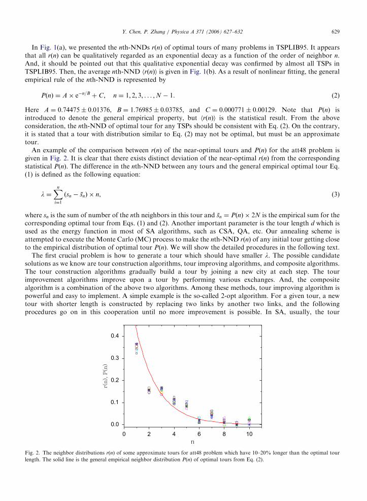
In Fig. 1(a), we presented the nth-NNDs rðnÞ of optimal tours of many problems in TSPLIB95. It appearsthat all rðnÞ can be qualitatively regarded as an exponential decay as a function of the order of neighbor n.And, it should be pointed out that this qualitative exponential decay was confirmed by almost all TSPs inTSPLIB95. Then, the average nth-NND hrðnÞi is given in Fig. 1(b). As a result of nonlinear fitting, the generalempirical rule of the nth-NND is represented by

PðnÞ ¼ A� e�n=B þ C; n ¼ 1; 2; 3; . . . ;N � 1. (2)

Here A ¼ 0:74475� 0:01376, B ¼ 1:76985� 0:03785, and C ¼ 0:000771� 0:00129. Note that PðnÞ isintroduced to denote the general empirical property, but hrðnÞi is the statistical result. From the aboveconsideration, the nth-NND of optimal tour for any TSPs should be consistent with Eq. (2). On the contrary,it is stated that a tour with distribution similar to Eq. (2) may not be optimal, but must be an approximatetour.

An example of the comparison between rðnÞ of the near-optimal tours and PðnÞ for the att48 problem isgiven in Fig. 2. It is clear that there exists distinct deviation of the near-optimal rðnÞ from the correspondingstatistical PðnÞ. The difference in the nth-NND between any tours and the general empirical optimal tour Eq.(1) is defined as the following equation:

l ¼Xn

i¼1

ðsn � s̄nÞ � n, (3)

where sn is the sum of number of the nth neighbors in this tour and s̄n ¼ PðnÞ � 2N is the empirical sum for thecorresponding optimal tour from Eqs. (1) and (2). Another important parameter is the tour length d which isused as the energy function in most of SA algorithms, such as CSA, QA, etc. Our annealing scheme isattempted to execute the Monte Carlo (MC) process to make the nth-NND rðnÞ of any initial tour getting closeto the empirical distribution of optimal tour PðnÞ. We will show the detailed procedures in the following text.

The first crucial problem is how to generate a tour which should have smaller l. The possible candidatesolutions as we know are tour construction algorithms, tour improving algorithms, and composite algorithms.The tour construction algorithms gradually build a tour by joining a new city at each step. The tourimprovement algorithms improve upon a tour by performing various exchanges. And, the compositealgorithm is a combination of the above two algorithms. Among these methods, tour improving algorithm ispowerful and easy to implement. A simple example is the so-called 2-opt algorithm. For a given tour, a newtour with shorter length is constructed by replacing two links by another two links, and the followingprocedures go on in this cooperation until no more improvement is possible. In SA, usually, the tour

Fig. 2. The neighbor distributions rðnÞ of some approximate tours for att48 problem which have 10–20% longer than the optimal tour

length. The solid line is the general empirical neighbor distribution PðnÞ of optimal tours from Eq. (2).

ARTICLE IN PRESSY. Chen, P. Zhang / Physica A 371 (2006) 627–632630

improving algorithm is embedded in Metropolis MC process to generate new tours at environmenttemperature.

In our algorithm, a similar mechanism is used to optimize a given tour by Metropolis MC process. We firstgenerate a random tour and set up a temperature which will be reduced very slowly. For every step, a new touris reconstructed from the old one by 3-exchange algorithm [20]. If Dlo0, where Dl ¼ lnew � lold , or e

�l=t isgreater than a random number between 0 and 1, the new tour is accepted. Repeated applications of this MCstep are carried out until l is smaller than lc, where lc means the acceptable difference between the neighbordistribution of the final tour and the empirical optimal PðnÞ from Eq. (2). Since it is impossible to offer theexact value of lc for each TSP, we usually keep running the annealing step until the tour length d cannot getsmaller.

Note that both our recipe and the CSA belong to the annealing scheme. The same MC steps are there, butour energy function is l different from the tour length d in CSA. Moreover, the corresponding configurationspace is absolutely different. We label our annealing scheme as l-space annealing, and rename the canonicalSA scheme as d-space annealing.

To measure the performances of the two distinct annealing strategies, we chose a standard TSP sample,eil101 problem, from the TSPLIB95 [19]. It is a N ¼ 101 cities problem constructed by Christofids and Eilonwhose optimal tour length dopt ¼ 629. Both l-space annealing and d-space annealing were applied to seeknear-optimal tours. Again, note that both annealing schemes begin with a random tour and make use of thesame 3-exchange algorithm. In Fig. 3, we present the detailed annealing processes in d-space and l-space. Theevolutions of tour length are described by Dd ¼ ðd � doptÞ=dopt � 100%. As it turns out, the final near-optimaltour for l-space annealing approximately coincides with d-space annealing (see Fig. 3(a) and (b)). But the l-space annealing is obviously faster than d-space annealing and note that the initial temperature in l-spaceannealing is far lower than in d-space annealing. In other words, l-space annealing works at small initialtemperature as well as at high initial temperature to make l of the tour smaller than the criterion lc. In fact,even 3-exchange technique can obtain a nice result, but it was highly dependent on the initial tours.

It is well known that the initial configuration with small temperature often causes trapping into localminimum too early. From Fig. 3, if someone uses d-space annealing to find a near-optimal tour with same Dd

resulting from l-space annealing, it should have a higher initial temperature and a longer annealing time. Sowe conjecture that the configuration space in l-space annealing is smoother than that in d-space annealing, orthe fluctuation in d-space annealing is stronger than that in l-space annealing. As a result, it is not necessarythat one uses the higher initial temperature to jump through energy valleys in l-space annealing.

However, it is very important to mention that d-space annealing can increase accuracy at the cost of higherinitial temperature and longer annealing time, but l-space annealing loses this property because it almostproduces a similar effect on annealing processes at higher or lower initial temperature for the more smoothl-space. It was concluded that l-space annealing can present approximate tours in shorter time, but it is verydifficult to improve its accuracy.

(a) (b)

Fig. 3. The detailed annealing processes in d-space annealing (SA) and l-space (OA) for eil101 problem in TSPLIB95. The insets are the

annealing details near optimal tour.

ARTICLE IN PRESSY. Chen, P. Zhang / Physica A 371 (2006) 627–632 631

In fact, the final tours obtained by l-space annealing are really different from the tours obtained by d-spaceannealing though both Dd’s apparently had very similar value of about 10% (see Fig. 3(a)). Taking the eil101problem as an example, the l of the approximate tour in d-space annealing is 730 and the l in l-spaceannealing is 260 (several other examples are presented in Table 1). The results in l-space annealing haveproperties of small d and small l. It means that l-space annealing can make d of the tours close to the optimaltour as well as make the neighbor distributions rðnÞ of tours close to PðnÞ. But in d-space annealing, the finalapproximate tours are restricted by the certain initial temperatures and their neighbor distributions are farfrom the distribution of optimal tour PðnÞ. Consequently, at a certain temperature, the annealing processes ind-space are easily trapped into local minimum and they lose the potential to find better tours in normalannealing schemes.

From the above statements, in d-space annealing, the tours usually have small d and large l at localminimum. Similarly, in l-space annealing, the tours normally have small d and small l, but they may not be inthe local minimum of d-space at certain temperatures. It suggests that one can design a combinationaloptimized SA in both d-space and l-space. As an example, it should be having higher potential to capturebetter tours when we take the tour obtained from l-space annealing as the initial tour in d-space annealing at acertain temperature. Theoretically, next, the annealing process can be moved onto l-space. This annealingprocess was repeated back and forth until the global optimal tour was found. SA in l-space and d-space byturns is the objective of our so-called optimized annealing scheme in this work. In fact, since the neighbordistribution of optimal tours PðnÞ is just a statistical rule, we perform a simple case of optimized annealingunder the name of ðlþ dÞ-space annealing, which is constructed by l-space annealing and d-space annealingonly once in this paper.

To get a comprehensive picture of the performance of our annealing schemes, we have calculated severalproblems in TSPLIB95, for N ¼ 48; 76; 101; 124; 136; 225; 532. The annealing results in d-space, l-space,ðlþ dÞ-space are listed at Table 1. Besides the confirmation of the above statements about Dd, l, andannealing velocity for d-space annealing and l-space annealing, it is highly important that ðlþ dÞ-spaceannealing is impressively superior to other annealing processes at each performance index.

In general, it is shown that our annealing recipe, especially ðlþ dÞ-space annealing, is far better than CSA.But it should be stated that the results are worsen with the growth of the city number N. It is believed that thesimple 3-exchange technique is not powerful enough to act on TSPs with large N. We emphasize the fact that,in this paper, we are not to pursue a perfect algorithm for the optimal tour, but to present a distinct andexcellent annealing technique.

In conclusion, for the symmetric TSPs, according to the statistical general property of the nth-nearest-neighbor distributions of the optimal tours, we define a new configuration space, so-called l-space, where ldescribes the difference between the neighbor distributions of any tours with the general rule, Eq. (2). Asindicated in simulation results, l-space annealing is more efficient than normal SA and the combination ofl-space annealing and CSA is more powerful. Further studies would be needed to clarify in more detail

Table 1

Annealing results in d-space, l-space, and ðlþ dÞ-space for some problems in TSPLIB95

Problems d-space l-space ðlþ dÞ-space

ðd � doptÞ

dopt

l MC steps ðd � doptÞ

dopt

l MC steps ðd � doptÞ

dopt

l MC steps

(%) ð�106Þ (%) ð�106Þ (%) ð�106Þ

Att48 5.1 230 3.0 5.0 30 0.8 0.1 169 0.2

Pr76 5.1 831 3.6 6.8 202 2.2 3.4 227 0.1

eil101 12.4 730 3.3 10.3 260 1.2 5.7 351 0.4

Pr107 7.3 800 2.3 7.1 272 2.0 4.7 373 0.2

Pr124 8.9 3138 3.0 16.2 359 0.1 8.5 499 0.2

Pr136 19.7 2958 1.1 19.1 623 0.5 13.0 1284 0.1

Ts225 22.2 8206 3.5 29.0 1037 0.6 14.7 1901 0.2

att532 43.0 176575 4.0 46.0 15376 1.0 28.0 20316 0.2

ARTICLE IN PRESSY. Chen, P. Zhang / Physica A 371 (2006) 627–632632

properties of the nth-NND and to seek for more valuable recipes for any TSPs even in the case of large N. Weexpect that this new general property, Eq. (2), can be combined with other techniques for TSP or otheroptimization problems.

Note that a similar distribution in the random link TSP and the Euclidean TSP was reported in Ref. [22]after we presented this work to axriv.

We thank Olivier Martin for pointing out Ref. [22]. The work reported in this paper was supported by theNational Natural Science Foundation of China under Grant no. 10305005 and the Special Fund for DoctorPrograms in Lanzhou University.

References

[1] E. Lawler, J.K. Lenstra, R. Khan, D. Shmoys, The Traveling Salesman Problem, Wiley, New York, 1985.

[2] C.H. Papadimitriou, K. Steiglitz, Combinatorial Optimization: Algorithms and Complexity, Prentice-Hall, Englewood Cliffs, NJ,

1982.

[3] See http://www.tsp.gatech.edu/

[4] M. Padberg, G. Rinaldi, Oper. Res. Lett. 6 (1987) 1.

[5] J.J. Hopfield, D.W. Tank, Biol. Cybern. 52 (1985) 141.

[6] S. Kirkpatrick, C.D. Gelatt, M.P. Vecchi, Science 220 (1983) 671.

[7] V. Cerny, J. Optim. Theory Appl. 45 (1985) 41.

[8] N. Kawashima, M. Suzuki, J. Phys. A 25 (1992) 1055.

[9] T. Nagatani, Phys. Rev. A 36 (1987) 5812.

[10] H. Nakanishi, F. Family, Phys. Rev. A 32 (1985) 3606.

[11] U. Yoshiyuki, K. Yoshiki, Phys. Rev. Lett. 75 (1995) 1683.

[12] R. Vgajin, Physica A 307 (2002) 260.

[13] S. Gemann, D. Gemann, IEEE Trans. Pattern Anal. Mach. Intell. PAMI-6 (1984) 721.

[14] H. Szu, R. Hartley, Phys. Lett. A 122 (1987) 157.

[15] D.A. Stariolo, C. Tsallis, in: D. Stauffer (Ed.), Annual Review of Computational Physics II, World Scientific, Singapore, 1994.

[16] T.J.P. Penna, Phys. Rev. E 51 (1995) R1.

[17] J. Brooke, D. Bitko, T.F. Rosenbaum, Science 284 (1999) 779.

[18] R. Martonak, G.E. Santoro, E. Tosatti, Phys. Rev. E 70 (2004) 057701.

[19] http://elib.zib.de/pub/Packages/mp-testdata/tsp/tsplib/tsplib.html

[20] S. Lin, Bell Syst. Tech. J. 44 (1965) 2245.

[21] O.C. Martin, S.W. Otto, Ann. Oper. Res. 63 (1996) 57.

[22] A.G. Percus, O.C. Martin, J. Stat. Phys. 94 (1999) 739.