optimize etl for the banking dds - sas support · pdf fileoptimize downstream etl in the...

Optimize ETL for the Banking DDS

Maximize and optimize downstream ETL when the banking

detail data store (DDS) is deployed in a database

Technical Paper

Technical Paper

Optimize Downstream ETL in the Banking DDS

Background

The banking DDS is an industry data model that provides an integrated data backplane for SAS Banking Solutions. The banking

DDS has been in development since early 2001, and the first production release was in 2004. Originally, the banking DDS

supported only SAS Customer Intelligence Solutions. It has grown consistently over time to support more solutions such as SAS

Customer Analytics for Banking, SAS Credit Scoring for Banking, SAS Credit Risk for Banking, and SAS Risk Management for

Banking.

Initially, the banking DDS was supported only in SAS data sets. Based on customer demand, the banking DDS is now supported

on SAS data sets, SAS Scalable Performance Data Server (SPD Server), Oracle, Teradata, DB2, and Microsoft SQL Server.

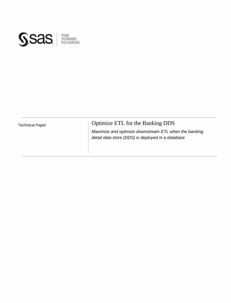
In the overall data flow, the banking DDS is the hub or data repository for downstream SAS solutions. ETL processes flow from the

banking DDS to the solution data marts, and some solutions have ETL processes that write back the results to the banking DDS.

Figure 1 shows the overall data flow.

EDW

Load

Extract and

Transform

So

urc

e S

yste

ms (O

LT

P/E

RP

etc

)

Extract and

Transform

Sta

gin

g A

rea

1

2

3

Enterprise Operational/

Data Warehouse Sources

Master

Data

Transaction

Data

ETL

ETL

ETL

Solution Data

Marts

SAS Detail Data

Store

4

5

6

SAS Solution

SAS Solution

SAS Solution

Solutions

Reference

Data

Write Back

Write Back

Write Back

Figure 1: Banking DDS Data Flow

2

The banking DDS uses two types of data flows—an acquisition ETL flow and a data delivery ETL flow.

Acquisition ETL Flows

The acquisition ETL flows (1, 2, and 3 in figure 1) acquire data from the source systems to populate the banking DDS tables.

Data Delivery ETL Flows

The data delivery ETL flows (4, 5, and 6 in figure 1) use the banking DDS as the source to populate the tables in the solution data

marts. Data delivery ETL is prebuilt and delivered to the customer with each SAS solution.

It is critical that the banking DDS and ETL processes be deployed for optimal performance. When the banking DDS data is not

stored in SAS data sets, optimizing performance requires special attention.

Overview

The intent of this project was to load data into the banking DDS tables in order to simulate a customer environment and learn how

to improve performance. ETL jobs deployed from SAS Risk Management for Banking were used in this project.

The banking DDS data model was deployed in SAS and three other database systems. Generated data was loaded to test the

different techniques for fine-tuning the data structure for the banking DDS and for improving the performance of selected ETL jobs.

Specifically, techniques that enabled the ETL jobs to run inside the databases were tested. The scope of the project focused on

what could be done by fine-tuning the ETL without rewriting the logic for the job.

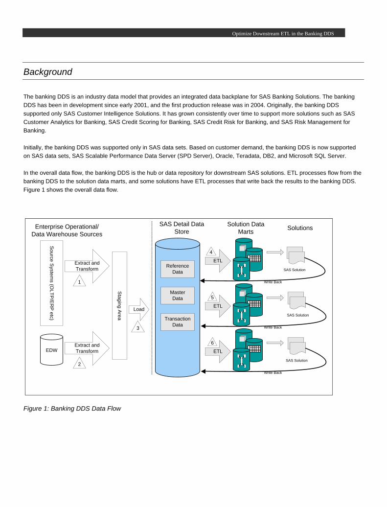
Project Setup

The project was set up with three tiers for the testing environment. All of the databases, except SAS, resided on its own server.

The SAS Metadata Server was set up on a separate server, and it also functioned as the SAS server. Separate client workstations

for managing the banking DDS and SAS Risk Management for Banking ETL metadata and for executing ETL jobs were

established.


Figure 2: Project Setup

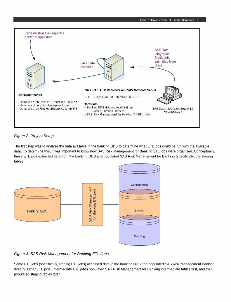
The first step was to analyze the data available in the banking DDS to determine what ETL jobs could be run with the available

data. To determine this, it was important to know how SAS Risk Management for Banking ETL jobs were organized. Conceptually,

these ETL jobs extracted data from the banking DDS and populated SAS Risk Management for Banking (specifically, the staging

tables).

Figure 3: SAS Risk Management for Banking ETL Jobs

Some ETL jobs (specifically, staging ETL jobs) accessed data in the banking DDS and populated SAS Risk Management Banking

directly. Other ETL jobs (intermediate ETL jobs) populated SAS Risk Management for Banking intermediate tables first, and then

populated staging tables later.

4

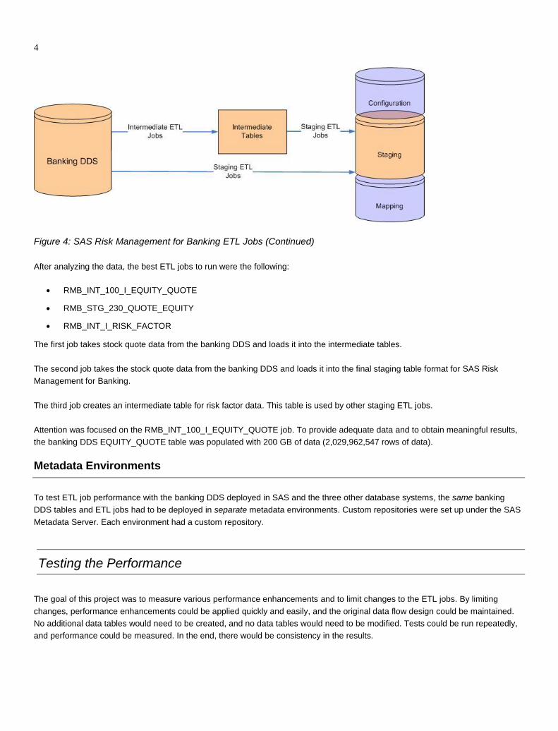
Figure 4: SAS Risk Management for Banking ETL Jobs (Continued)

After analyzing the data, the best ETL jobs to run were the following:

RMB_INT_100_I_EQUITY_QUOTE

RMB_STG_230_QUOTE_EQUITY

RMB_INT_I_RISK_FACTOR

The first job takes stock quote data from the banking DDS and loads it into the intermediate tables.

The second job takes the stock quote data from the banking DDS and loads it into the final staging table format for SAS Risk

Management for Banking.

The third job creates an intermediate table for risk factor data. This table is used by other staging ETL jobs.

Attention was focused on the RMB_INT_100_I_EQUITY_QUOTE job. To provide adequate data and to obtain meaningful results,

the banking DDS EQUITY_QUOTE table was populated with 200 GB of data (2,029,962,547 rows of data).

Metadata Environments

To test ETL job performance with the banking DDS deployed in SAS and the three other database systems, the same banking

DDS tables and ETL jobs had to be deployed in separate metadata environments. Custom repositories were set up under the SAS

Metadata Server. Each environment had a custom repository.

Testing the Performance

The goal of this project was to measure various performance enhancements and to limit changes to the ETL jobs. By limiting

changes, performance enhancements could be applied quickly and easily, and the original data flow design could be maintained.

No additional data tables would need to be created, and no data tables would need to be modified. Tests could be run repeatedly,

and performance could be measured. In the end, there would be consistency in the results.


Out-of-the-Box ETL Jobs

The ETL jobs provided with SAS Risk Management for Banking populated three general types of tables: the underlying work tables

that were created in SAS Data Integration Studio, the intermediate tables, and the staging tables. For the first test, the banking

DDS tables and all of the downstream tables (work, intermediate, and staging) were deployed on SAS. Then, in three separate

tests, all of the tables were deployed on each of three different database systems. In the following examples, attention was focused

on one ETL job that created the intermediate table that provided the equity quote data for SAS Risk Management for Banking.

Figure 5: Workflow of RMB_INT_100_I_EQUITY_QUOTE Job

The RMB_INT_100_I_EQUITY_QUOTE job extracted all rows of the data and a subset of columns and loaded the data into a

temporary data set. This data was aggregated by the max quote data into a second temporary data set, and then joined with the

source DDS data table to extract additional columns. As a result, a third and final temporary data set was created and loaded into

an intermediate table. The logical workflow is shown in Figure 6. Optimizing this ETL job depended on the locations of the source

and target data in the environment. Localizing the transfer of data from one table to another was the key to optimal performance.

And, the original data flow design was maintained.

Figure 6: Logical Workflow of RMB_INT_100_I_EQUITY_QUOTE Job

In this project, SAS code was extracted from the job and then modified. This choice localized the processing to the database,

instead of SAS performing processing outside of the database. For this to happen, PROC SQL code was rewritten to use in-

database processing or explicit pass-through. Explicit pass-through is invaluable in the event of implicit SQL query disqualification.

Disqualification occurs when the code violates implicit pass-through rules. In the following figure, the differences between implicit

pass-through and explicit pass-through are shown.

6

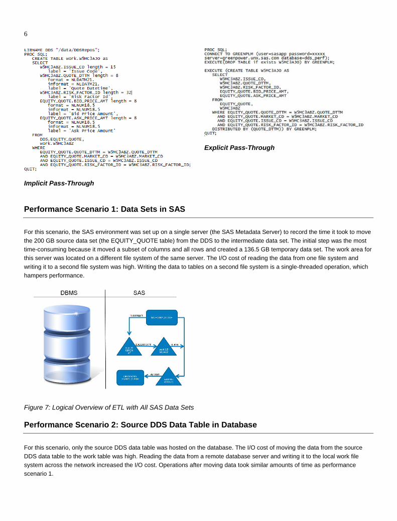
Implicit Pass-Through

Explicit Pass-Through

Performance Scenario 1: Data Sets in SAS

For this scenario, the SAS environment was set up on a single server (the SAS Metadata Server) to record the time it took to move

the 200 GB source data set (the EQUITY_QUOTE table) from the DDS to the intermediate data set. The initial step was the most

time-consuming because it moved a subset of columns and all rows and created a 136.5 GB temporary data set. The work area for

this server was located on a different file system of the same server. The I/O cost of reading the data from one file system and

writing it to a second file system was high. Writing the data to tables on a second file system is a single-threaded operation, which

hampers performance.

Figure 7: Logical Overview of ETL with All SAS Data Sets

Performance Scenario 2: Source DDS Data Table in Database

For this scenario, only the source DDS data table was hosted on the database. The I/O cost of moving the data from the source

DDS data table to the work table was high. Reading the data from a remote database server and writing it to the local work file

system across the network increased the I/O cost. Operations after moving data took similar amounts of time as performance

scenario 1.


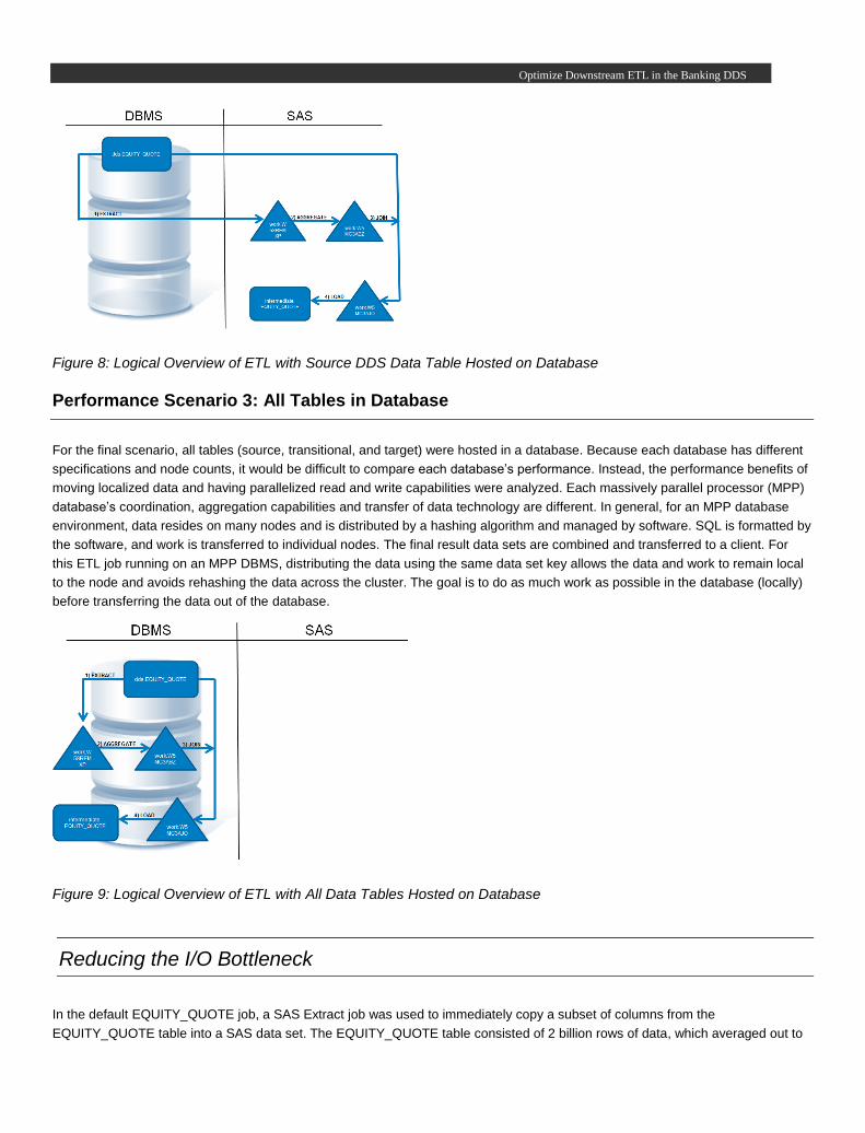
Figure 8: Logical Overview of ETL with Source DDS Data Table Hosted on Database

Performance Scenario 3: All Tables in Database

For the final scenario, all tables (source, transitional, and target) were hosted in a database. Because each database has different

specifications and node counts, it would be difficult to compare each database’s performance. Instead, the performance benefits of

moving localized data and having parallelized read and write capabilities were analyzed. Each massively parallel processor (MPP)

database’s coordination, aggregation capabilities and transfer of data technology are different. In general, for an MPP database

environment, data resides on many nodes and is distributed by a hashing algorithm and managed by software. SQL is formatted by

the software, and work is transferred to individual nodes. The final result data sets are combined and transferred to a client. For

this ETL job running on an MPP DBMS, distributing the data using the same data set key allows the data and work to remain local

to the node and avoids rehashing the data across the cluster. The goal is to do as much work as possible in the database (locally)

before transferring the data out of the database.

Figure 9: Logical Overview of ETL with All Data Tables Hosted on Database

Reducing the I/O Bottleneck

In the default EQUITY_QUOTE job, a SAS Extract job was used to immediately copy a subset of columns from the

EQUITY_QUOTE table into a SAS data set. The EQUITY_QUOTE table consisted of 2 billion rows of data, which averaged out to

8

be ~200 GB of data. This extraction of data required creating approximately 2 billion rows in a SAS data set. The I/O cost of this

job was severe. And, the job’s performance was heavily impeded. After the data was moved into SAS, the various tasks in the SAS

Extract job took considerably less time. The following figure shows the workflow of and the different tasks in the SAS Extract job.

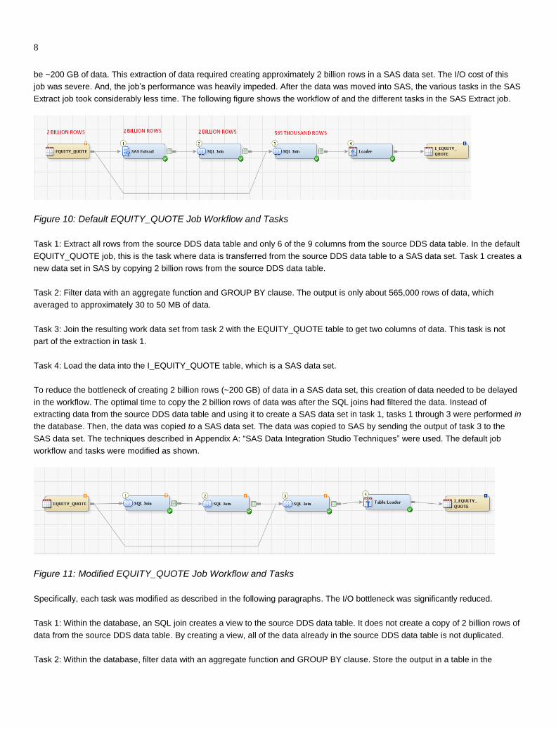
Figure 10: Default EQUITY_QUOTE Job Workflow and Tasks

Task 1: Extract all rows from the source DDS data table and only 6 of the 9 columns from the source DDS data table. In the default

EQUITY_QUOTE job, this is the task where data is transferred from the source DDS data table to a SAS data set. Task 1 creates a

new data set in SAS by copying 2 billion rows from the source DDS data table.

Task 2: Filter data with an aggregate function and GROUP BY clause. The output is only about 565,000 rows of data, which

averaged to approximately 30 to 50 MB of data.

Task 3: Join the resulting work data set from task 2 with the EQUITY_QUOTE table to get two columns of data. This task is not

part of the extraction in task 1.

Task 4: Load the data into the I_EQUITY_QUOTE table, which is a SAS data set.

To reduce the bottleneck of creating 2 billion rows (~200 GB) of data in a SAS data set, this creation of data needed to be delayed

in the workflow. The optimal time to copy the 2 billion rows of data was after the SQL joins had filtered the data. Instead of

extracting data from the source DDS data table and using it to create a SAS data set in task 1, tasks 1 through 3 were performed in

the database. Then, the data was copied to a SAS data set. The data was copied to SAS by sending the output of task 3 to the

SAS data set. The techniques described in Appendix A: “SAS Data Integration Studio Techniques” were used. The default job

workflow and tasks were modified as shown.

Figure 11: Modified EQUITY_QUOTE Job Workflow and Tasks

Specifically, each task was modified as described in the following paragraphs. The I/O bottleneck was significantly reduced.

Task 1: Within the database, an SQL join creates a view to the source DDS data table. It does not create a copy of 2 billion rows of

data from the source DDS data table. By creating a view, all of the data already in the source DDS data table is not duplicated.

Task 2: Within the database, filter data with an aggregate function and GROUP BY clause. Store the output in a table in the


database. The output includes about 565,000 rows (approximately 30 to 50 MB).

Task 3: Join the resulting in-database data set from task 2 with the EQUITY_QUOTE table to get two columns of data. This task is

not part of the extraction in task 1. The output of this task is loaded into a SAS data set. The I/O cost is reduced because only

565,000 rows of data are created, not 2 billion. In summary, only 30 to 50 MB of data was moved instead of 200 GB.

Task 4: Load the data into the I_EQUITY_QUOTE table, which is a SAS data set.

Conclusions

In our testing, minimal changes were made to the source DDS data table (EQUITY_QUOTE). The ETL jobs that were tested used

the highest volume of data that was available. By using the EQUITY_QUOTE table (the largest source DDS data table), the ETL

job had minimal filter and join conditions. This information governed how data was distributed in an MPP database. The sample

data had the highest cardinality data in the QUOTE_DTTM column. This made the QUOTE_DTTM column a good candidate for

the distribution key. Because data is different for each customer, there is no one-size-fits-all method for optimizing performance.

The strategy should be to minimize I/O by localizing the work, intermediate, and stage tables. If tables can be localized, there will

be a performance improvement.

The default ETL job created many data sets. Then, data was moved from one location to another. Moving this data caused the

largest I/O bottleneck. The largest move within this I/O bottleneck was the initial move of data from a 200 GB source DDS data

table to a 136.5 GB SAS data set. By localizing the data and moving it from one table to another table within the database, or by

removing the data move all together by creating a view to the database, job time was cut drastically.

The results are displayed in the following table. Each database environment was running on different hardware. In these results, it

is more important to see the individual gain in performance, not a comparison of performance. So, the databases are not labeled

so that they are not compared. SAS values are provided as benchmarks.

Database

Total Average Time for Non-Optimized ETL (in hours)

Total Average Time for Optimized ETL (in hours) Performance Gain Total (in

hours)

SAS 1.65 N/A N/A

Database A Over 8.00 0.10 Over 8.00

Database B 6.58 0.13 6.59

Database C Over 8.00 1.62 Over 8.00

SAS solutions such as SAS Risk Management for Banking often include out-of-the-box ETL jobs. When either the source table or

the target table of these ETL jobs is changed from a SAS data set to a database table, ETL performance is affected. In our testing,

we dramatically improved ETL performance in SAS Risk Management for Banking by making minor changes to the ETL jobs

provided with the solution. Although these changes were made to a specific set of ETL jobs, the underlying techniques can be used

to change any ETL job. The bottom line is performance is optimized when ETL code executes in the database.

10

Appendix A: SAS Data Integration Studio Techniques

This appendix describes the SAS Data Integration Studio techniques that were used to change the out-of-the-box jobs to execute

in a database.

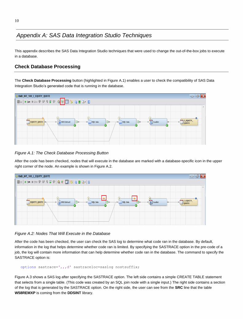
Check Database Processing

The Check Database Processing button (highlighted in Figure A.1) enables a user to check the compatibility of SAS Data

Integration Studio’s generated code that is running in the database.

Figure A.1: The Check Database Processing Button

After the code has been checked, nodes that will execute in the database are marked with a database-specific icon in the upper

right corner of the node. An example is shown in Figure A.2.

Figure A.2: Nodes That Will Execute in the Database

After the code has been checked, the user can check the SAS log to determine what code ran in the database. By default,

information in the log that helps determine whether code ran is limited. By specifying the SASTRACE option in the pre-code of a

job, the log will contain more information that can help determine whether code ran in the database. The command to specify the

SASTRACE option is:

options sastrace=',,,d' sastraceloc=saslog nostsuffix;

Figure A.3 shows a SAS log after specifying the SASTRACE option. The left side contains a simple CREATE TABLE statement

that selects from a single table. (This code was created by an SQL join node with a single input.) The right side contains a section

of the log that is generated by the SASTRACE option. On the right side, the user can see from the SRC line that the table

W58REMXP is coming from the DDSINT library.


Figure A.3: SQL Join with Single Input (left) and Output Generated by the SASTRACE Option (right)

Replace SAS Extract with SQL Join

In SAS Data Integration Studio, the SAS Extract job is not supported to completely execute in the database. If the user clicks the

Check Database Processing button, the message “Unable to completely process on [database]” will appear. A workaround is to

replace the SAS Extract job with an SQL join that has a single input. By having a single input to the SQL join, the same logical

functionality of the SAS Extract job is performed, and the ability to generate SAS pass-through code is gained. By default, an SQL

Join node has two input ports. To emulate the SAS Extract job, one input port must be removed. Figure A.4 shows how to remove

the extra input port.

Figure A.4: Removing an Extra Input Port

12

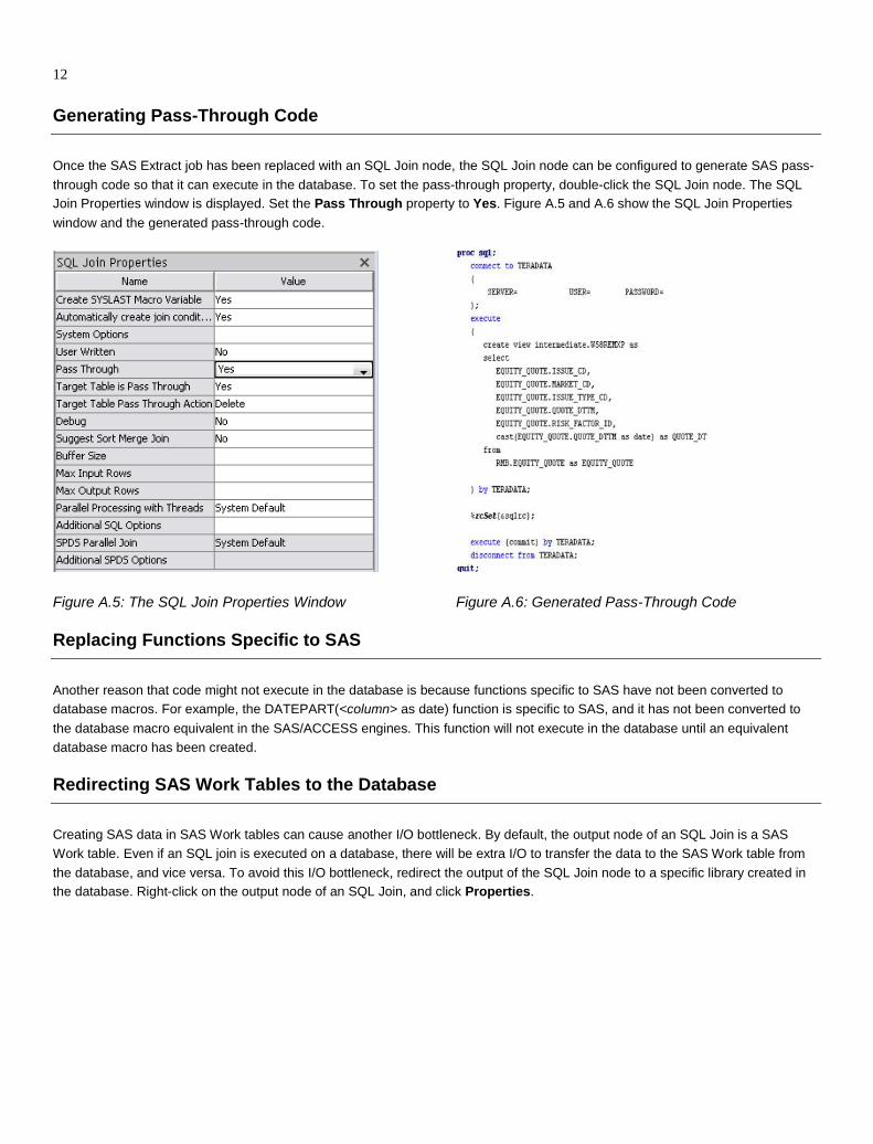
Generating Pass-Through Code

Once the SAS Extract job has been replaced with an SQL Join node, the SQL Join node can be configured to generate SAS pass-

through code so that it can execute in the database. To set the pass-through property, double-click the SQL Join node. The SQL

Join Properties window is displayed. Set the Pass Through property to Yes. Figure A.5 and A.6 show the SQL Join Properties

window and the generated pass-through code.

Figure A.5: The SQL Join Properties Window Figure A.6: Generated Pass-Through Code

Replacing Functions Specific to SAS

Another reason that code might not execute in the database is because functions specific to SAS have not been converted to

database macros. For example, the DATEPART(<column> as date) function is specific to SAS, and it has not been converted to

the database macro equivalent in the SAS/ACCESS engines. This function will not execute in the database until an equivalent

database macro has been created.

Redirecting SAS Work Tables to the Database

Creating SAS data in SAS Work tables can cause another I/O bottleneck. By default, the output node of an SQL Join is a SAS

Work table. Even if an SQL join is executed on a database, there will be extra I/O to transfer the data to the SAS Work table from

the database, and vice versa. To avoid this I/O bottleneck, redirect the output of the SQL Join node to a specific library created in

the database. Right-click on the output node of an SQL Join, and click Properties.


Figure A.7: Select Properties

After the SQL Join Properties window appears, click the Physical Storage tab, and change Location from Job’s default library

for temporary tables to Redirect to a registered library. Choose the same database library that you are using for the source

DDS data table.

Figure A.8: Redirect the Output

optimize etl for the banking dds - sas support · pdf fileoptimize downstream etl in the...

Documents