optimizationforml linear*regressionmgormley/courses/10601-s17/slides/... · optimizationforml +...
TRANSCRIPT
Optimization for ML+
Linear Regression
1
10-‐601 Introduction to Machine Learning
Matt GormleyLecture 7
February 8, 2016
Machine Learning DepartmentSchool of Computer ScienceCarnegie Mellon University
Optimization Readings:Lecture notes from 10-‐600 (see Piazza note)
“Convex Optimization” Boyd and Vandenberghe (2009) [See Chapter 9. This advanced reading is entirely optional.]
Linear Regression Readings:Murphy 7.1 – 7.3Bishop 3.1HTF 3.1 – 3.4Mitchell 4.1-‐4.3

Reminders
• Homework 2: Naive Bayes– Release: Wed, Feb. 1– Due: Mon, Feb. 13 at 5:30pm
• Homework 3: Linear / Logistic Regression– Release: Mon, Feb. 13– Due: Wed, Feb. 22 at 5:30pm
2

Optimization Outline• Optimization for ML
– Differences – Types of optimization problems– Unconstrained optimization– Convex, concave, nonconvex
• Optimization: Closed form solutions– Example: 1-‐D function– Example: higher dimensions– Gradient and Hessian
• Gradient Descent– Example: 2D gradients– Algorithm– Details: starting point, stopping criterion, line search
• Stochastic Gradient Descent (SGD)– Expectations of gradients– Algorithm– Mini-‐batches– Details: mini-‐batches, step size, stopping criterion– Problematic cases for SGD
• Convergence– Comparison of Newton’s method, Gradient Descent, SGD– Asymptotic convergence– Convergence in practice
3
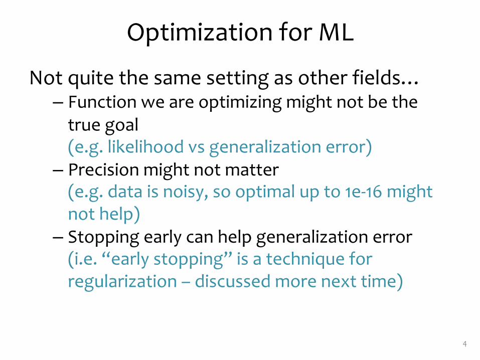
Optimization for ML
Not quite the same setting as other fields…– Function we are optimizing might not be the true goal (e.g. likelihood vs generalization error)
– Precision might not matter (e.g. data is noisy, so optimal up to 1e-‐16 might not help)
– Stopping early can help generalization error(i.e. “early stopping” is a technique for regularization – discussed more next time)
4

Optimization for ML
Whiteboard– Differences – Types of optimization problems– Unconstrained optimization– Convex, concave, nonconvex
5
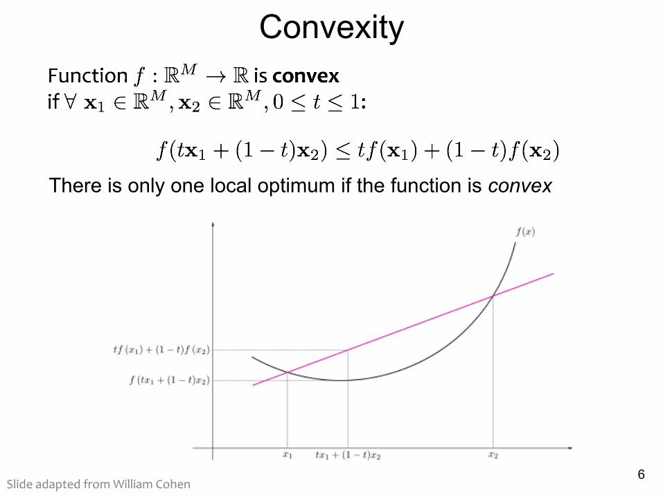
Convexity
6
There is only one local optimum if the function is convex
Slide adapted from William Cohen
Optimization: Closed form solutions
Whiteboard– Example: 1-‐D function– Example: higher dimensions– Gradient and Hessian
7
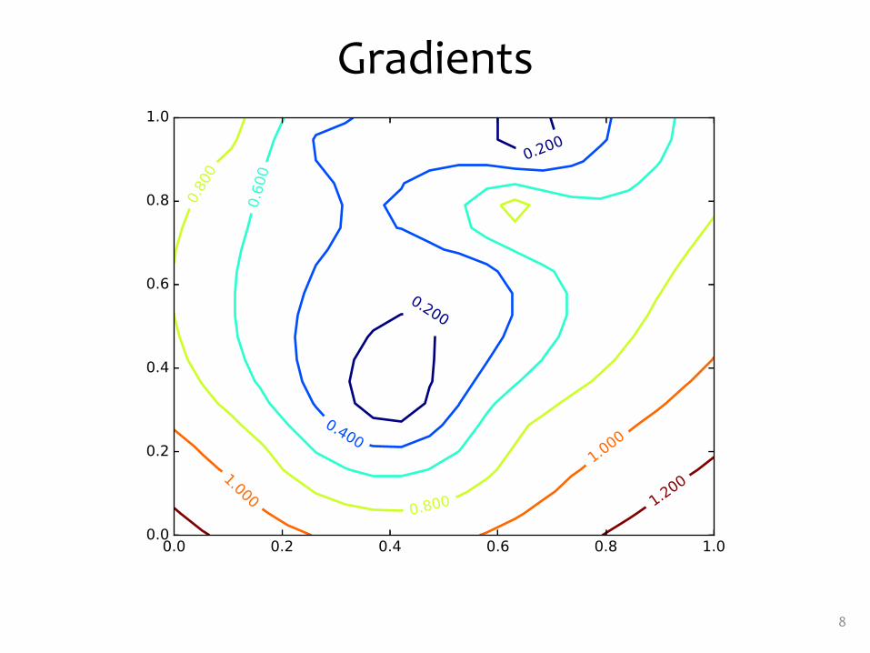
Gradients
8

Gradients
9These are the gradients that Gradient Ascent would follow.
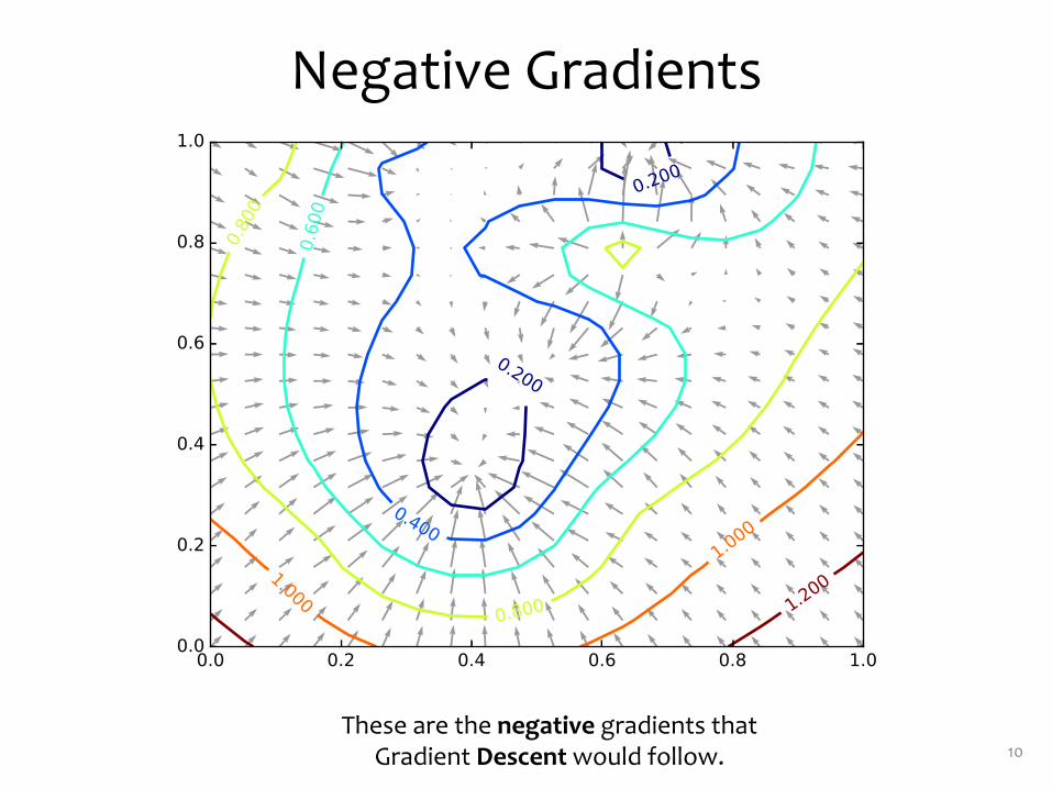
Negative Gradients
10These are the negative gradients that
Gradient Descentwould follow.
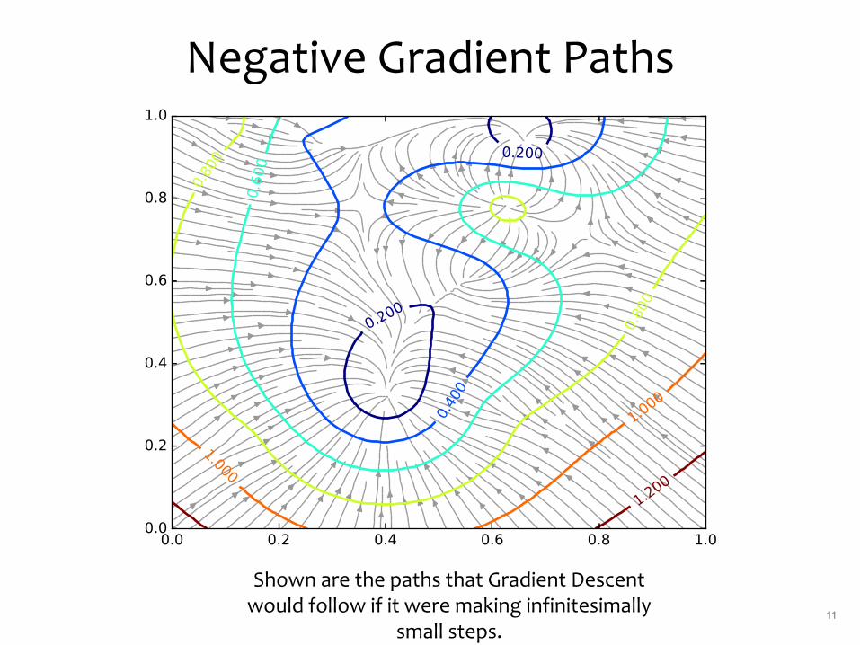
Negative Gradient Paths
11
Shown are the paths that Gradient Descent would follow if it were making infinitesimally
small steps.
Gradient Descent
Whiteboard– Example: 2D gradients– Algorithm– Details: starting point, stopping criterion, line search
12
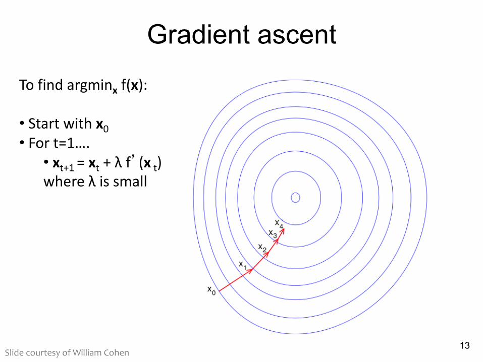
Gradient ascent
13
To find argminx f(x):
• Start with x0• For t=1….• xt+1 = xt + λ f’(x t)where λ is small
Slide courtesy of William Cohen
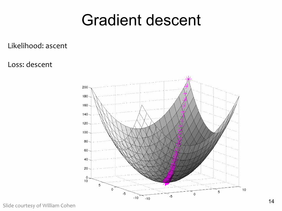
Gradient descent
14
Likelihood: ascent
Loss: descent
Slide courtesy of William Cohen
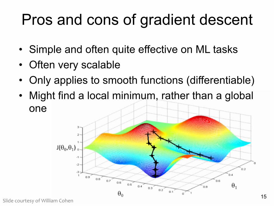
Pros and cons of gradient descent
• Simple and often quite effective on ML tasks• Often very scalable • Only applies to smooth functions (differentiable)• Might find a local minimum, rather than a global one
15Slide courtesy of William Cohen

Gradient Descent
16
Algorithm 1 Gradient Descent
1: procedure GD(D, �(0))2: � � �(0)
3: while not converged do4: � � � + ���J(�)
5: return �
In order to apply GD to Linear Regression all we need is the gradient of the objective function (i.e. vector of partial derivatives).
��J(�) =
�
����
dd�1
J(�)d
d�2J(�)...
dd�N
J(�)
�
����
—
Gradient Descent
17
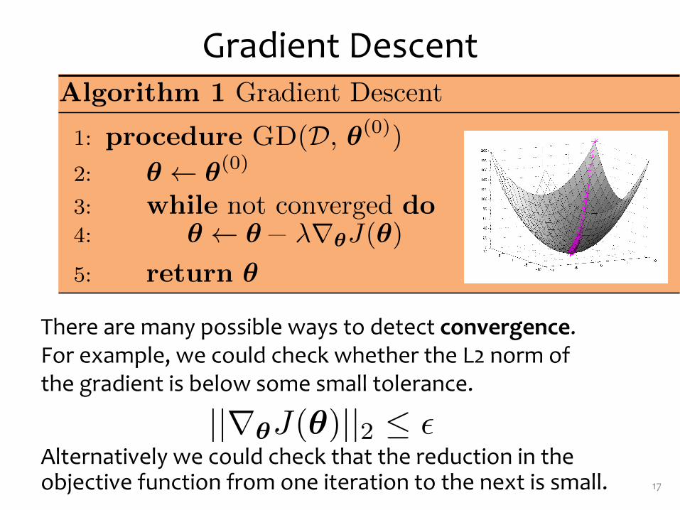
Algorithm 1 Gradient Descent
1: procedure GD(D, �(0))2: � � �(0)
3: while not converged do4: � � � + ���J(�)
5: return �
There are many possible ways to detect convergence. For example, we could check whether the L2 norm of the gradient is below some small tolerance.
||��J(�)||2 � �Alternatively we could check that the reduction in the objective function from one iteration to the next is small.
—
Stochastic Gradient Descent (SGD)
Whiteboard– Expectations of gradients– Algorithm–Mini-‐batches– Details: mini-‐batches, step size, stopping criterion
– Problematic cases for SGD
18

Stochastic Gradient Descent (SGD)
19
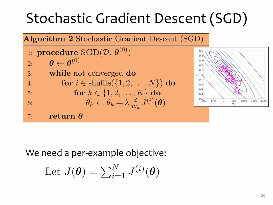
Algorithm 2 Stochastic Gradient Descent (SGD)
1: procedure SGD(D, �(0))2: � � �(0)
3: while not converged do4: for i � shu�e({1, 2, . . . , N}) do5: � � � + ���J (i)(�)
6: return �
We need a per-‐example objective:
Let J(�) =�N
i=1 J (i)(�)where J (i)(�) = 1
2 (�T x(i) � y(i))2.
—
Stochastic Gradient Descent (SGD)
We need a per-‐example objective:
20
Let J(�) =�N
i=1 J (i)(�)where J (i)(�) = 1
2 (�T x(i) � y(i))2.
Algorithm 2 Stochastic Gradient Descent (SGD)
1: procedure SGD(D, �(0))2: � � �(0)
3: while not converged do4: for i � shu�e({1, 2, . . . , N}) do5: for k � {1, 2, . . . , K} do6: �k � �k + � d
d�kJ (i)(�)
7: return �
—
Convergence
Whiteboard– Comparison of Newton’s method, Gradient Descent, SGD
– Asymptotic convergence– Convergence in practice
21
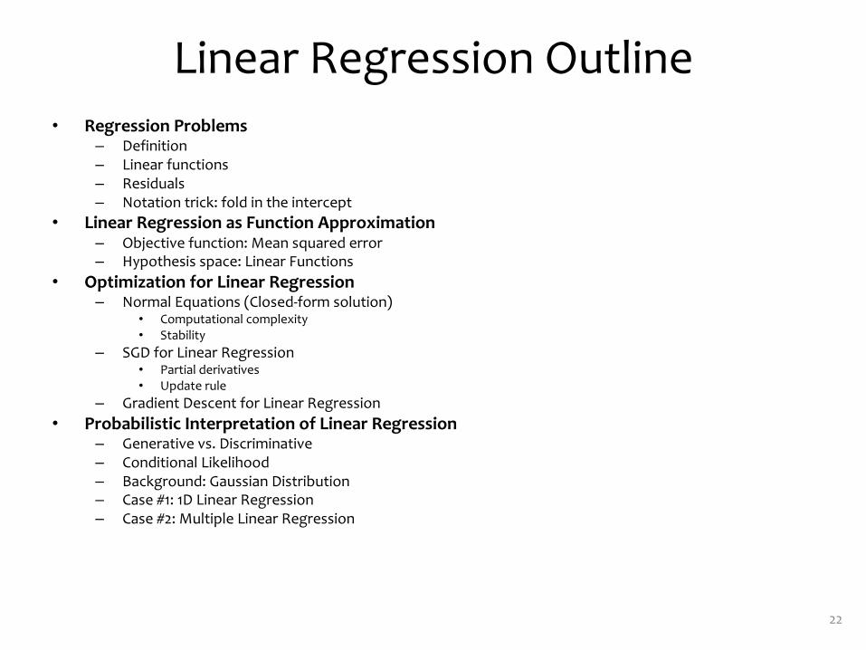
Linear Regression Outline• Regression Problems
– Definition– Linear functions– Residuals– Notation trick: fold in the intercept
• Linear Regression as Function Approximation– Objective function: Mean squared error– Hypothesis space: Linear Functions
• Optimization for Linear Regression– Normal Equations (Closed-‐form solution)
• Computational complexity• Stability
– SGD for Linear Regression• Partial derivatives• Update rule
– Gradient Descent for Linear Regression• Probabilistic Interpretation of Linear Regression
– Generative vs. Discriminative– Conditional Likelihood– Background: Gaussian Distribution– Case #1: 1D Linear Regression– Case #2: Multiple Linear Regression
22

Regression Problems
Whiteboard– Definition– Linear functions– Residuals– Notation trick: fold in the intercept
23

Linear Regression as Function Approximation
Whiteboard– Objective function: Mean squared error– Hypothesis space: Linear Functions
24
Optimization for Linear Regression
Whiteboard– Normal Equations (Closed-‐form solution)• Computational complexity• Stability
– SGD for Linear Regression• Partial derivatives• Update rule
– Gradient Descent for Linear Regression
25

Probabilistic Interpretation of Linear Regression
Whiteboard– Generative vs. Discriminative– Conditional Likelihood– Background: Gaussian Distribution– Case #1: 1D Linear Regression– Case #2: Multiple Linear Regression
26
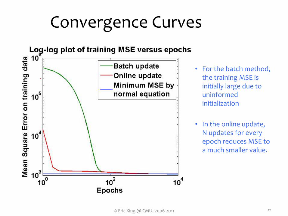
Convergence Curves
• For the batch method, the training MSE is initially large due to uninformed initialization
• In the online update, N updates for every epoch reduces MSE to a much smaller value.
27© Eric Xing @ CMU, 2006-‐2011