optimization with missing data - university of southamptonaijf197/rspa20051608p.pdf · optimization...

Optimization with missing data

BY ALEXANDER I. J. FORRESTER*, ANDRAS SOBESTER

AND ANDY J. KEANE

Computational Engineering and Design Group, School of Engineering Sciences,University of Southampton, Southampton SO17 1BJ, UK

Engineering optimization relies routinely on deterministic computer based designevaluations, typically comprising geometry creation, mesh generation and numericalsimulation. Simple optimization routines tend to stall and require user intervention if afailure occurs at any of these stages. This motivated us to develop an optimizationstrategy based on surrogate modelling, which penalizes the likely failure regions of thedesign space without prior knowledge of their locations. A Gaussian process based designimprovement expectation measure guides the search towards the feasible global optimum.

Keywords: global optimization; imputation; Kriging

*A

RecAcc

1. Introduction

New areas of research or the early stages of a design process require a geometrymodel, with coupled analysis codes, which encompasses a wide range of possibledesigns. In such situations the analysis code is likely to fail to return results forsome configurations due to a variety of reasons. Problems may occur at any stageof the design evaluation process: (i) the geometry described by a parametercombination may be infeasible, (ii) an automated mesh generator may not beable to cope with a particularly complex or corrupt geometry or (iii) thesimulation may not converge, either due to mesh problems or the automatedsolution setup being unable to cope with certain unusual, yet geometricallyfeasible, configurations.

In an ideal world, a seamless parameterization would ensure that the optimizercould visit wide ranging geometries and move between them without interruption.In reality, however, the uniform, flawless coverage of the design space by a genericgeometry model and simulation procedure is fraught with difficulties. In all butthe most trivial or over-constrained cases the design evaluation can fail in certainareas of the search space. Of course, if these infeasible areas are rectangular, theycan simply be avoided by adjusting the bounds of the relevant variables, but thisis rarely the case. Most of the time such regions will have complex, irregular, andeven disconnected shapes, and are much harder to identify and avoid. In thepresence of such problems it is difficult to accomplish entirely automatedoptimization without narrowing the bounds of the problem to the extent thatpromising designs are likely to be excluded. This negates the possible benefits of

Proc. R. Soc. A (2006) 462, 935–945

doi:10.1098/rspa.2005.1608

Published online 10 January 2006

uthor for correspondence ([email protected]).

eived 29 June 2005epted 1 November 2005 935 q 2006 The Royal Society

A. I. J. Forrester and others936

global optimization routines, and the designer may well choose to revert to a moreconservative local optimization around a known good design.

Although industry and academia direct considerable effort at robust geometrycreation and mesh generation, it is unlikely that truly fault free automated designevaluation will be achieved. Rather than tackling problems with the individualdesign evaluation components, we address, or rather circumvent, the problem offailed design evaluations via the medium of surrogate based optimizationmethodology. This approach allows us to cope with regions of infeasible designswithout knowingwhere theywill occur. Although gradient-free searchmethods, forexample a genetic algorithm (GA), can complete a global search of a domain withinfeasible regions, the large number of direct calls to the computer code will rendersuch methods impractical when using time consuming simulations, as shown whenwe compare the performance of our surrogate based methods with a GA in §4.

We begin in the next section by presenting the surrogate modelling basedoptimization approach we use in this paper. The following section discusses theproblems associated with failed design evaluations and introduces the proposedsolution methodology. We go on in §4 to demonstrate our method on an aerofoildesign case study, before drawing conclusions in the final section.

2. Surrogate based optimization

This paper is centred around surrogate based optimization, and as such we begin

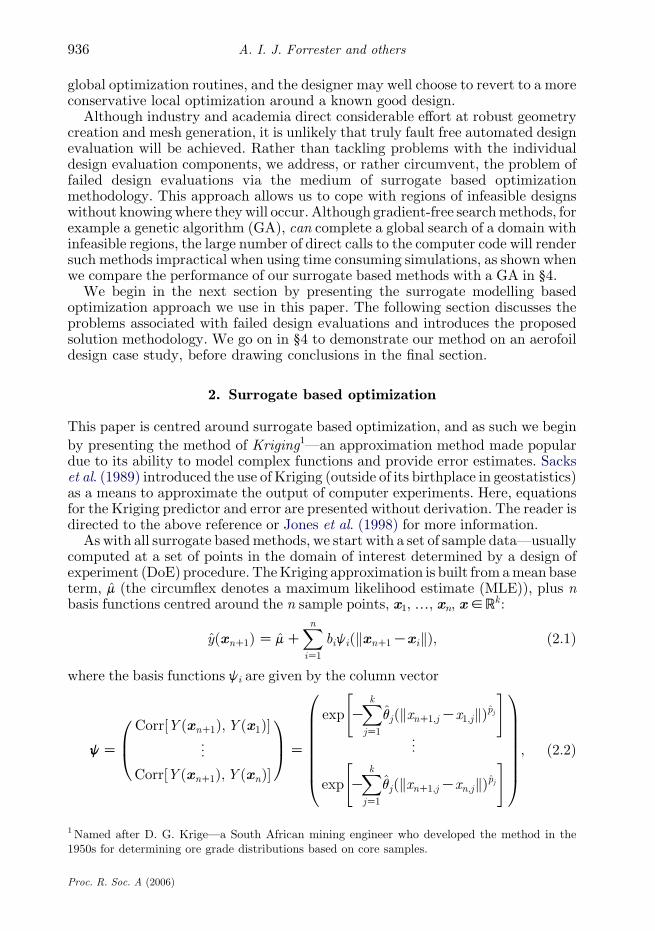
by presenting the method of Kriging1—an approximation method made populardue to its ability to model complex functions and provide error estimates. Sackset al. (1989) introduced the use of Kriging (outside of its birthplace in geostatistics)as a means to approximate the output of computer experiments. Here, equationsfor the Kriging predictor and error are presented without derivation. The reader isdirected to the above reference or Jones et al. (1998) for more information.

As with all surrogate basedmethods, we start with a set of sample data—usuallycomputed at a set of points in the domain of interest determined by a design ofexperiment (DoE) procedure. TheKriging approximation is built from amean baseterm, m (the circumflex denotes a maximum likelihood estimate (MLE)), plus nbasis functions centred around the n sample points, x1,., xn, x2R

k:

yðxnC1ÞZ mCXniZ1

bijiðkxnC1KxikÞ; ð2:1Þ

where the basis functions ji are given by the column vector

jZ

Corr½Y ðxnC1Þ;Y ðx1Þ�«

Corr½Y ðxnC1Þ;Y ðxnÞ�

0B@1CAZ

exp KXkjZ1

qjðkxnC1;jKx1;jkÞpj" #

«

exp KXkjZ1

qjðkxnC1;jKxn;jkÞpj" #

0BBBBBBB@

1CCCCCCCA; ð2:2Þ

1 Named after D. G. Krige—a South African mining engineer who developed the method in the1950s for determining ore grade distributions based on core samples.

Proc. R. Soc. A (2006)

937Optimization with missing data

(the correlation between a randomvariableY(x) at the point to be predicted (xnC1)and at the sample data points (x1,., xn)). The hyper-parameter pj can be thoughtof as determining the smoothness of the function approximation. In geostatisticalmodels, where Kriging originated, erratic local behaviour (the nugget effect) maybenefit from the use of pj2½0;1� to allow for erratic responses, but here themodelling of engineering functions implies that there will not be any singularitiesand the use of pjZ2means that the basis function is infinitely differentiable througha sample point (when kxnC1KxikZ0). With pjZ2, the basis function has aGaussian distribution with variance 1=qj . q, therefore, can be thought of as

determining how quickly the function changes as xnC1 moves away from xi , withhigh and low qjs indicating an active or inactive function, respectively. It is usualpractice to use a constant qj for all dimensions in x, but the use of variable qjs gives anon-axisymmetric basis, allowing for varying impacts of each variable of the designspace. In essence, the variance 1=qj is used to normalize the distance kxnC1;jKxi;jkto give equal activity across each dimension Jones et al. (1998).

The constants bi are given by the column vector bZRK1ðyK1mÞ, where R isan n!n symmetric matrix of correlations between the sample data, y is a columnvector of the sample data, ðyðx1Þ;.; yðxnÞÞT, 1 is an n!1 column vector of ones,

and the MLE prediction of mZ1TRK1y=1TRK11.In addition to computing an initial set of experiments and fitting an

approximation to the data, the surface is usually refined with additional data(update or infill points) to improve accuracy in the area of the optimum andconfirm the objective function values predicted by the approximation. A naturalway of refining the surface is to compute a new simulation at the predictedoptimum. The approximation is then rebuilt and new optimum points are addeduntil the predicted optimum agrees with the update simulation to a specifiedtolerance. The optimization may, however, become ‘trapped’ at local optimawhen searching multi-modal functions (see Jones (2001) for an excellent review ofthe pitfalls of various update criteria). An update strategy must allow for theprediction being just that—a prediction. The Kriging predictor, yðxnC1Þ, ischosen to maximize the likelihood of the combined test data and prediction (theaugmented likelihood). It follows that predicted values are likely to be moreaccurate if the likelihood drops off sharply as the value of yðxnC1Þ changes, i.e.alternative values are inconsistent with the initial dataset. Conversely, a gentledrop-off in the likelihood indicates that alternative values of yðxnC1Þ are morelikely to be possible. This notion leads to an intuitive method of deriving theestimated mean squared error in the predictor. The curvature of the augmentedlikelihood is found by taking the second derivative with respect to yðxnC1Þ, and itfollows that the error in the predictor is related to the inverse of this curvature:

s2ðxnC1ÞZ bs2 ½1KjTRK1j�; ð2:3Þwhere bs2ZðyK1mÞTRK1ðyK1mÞ=n. The full, though rather less revealingderivation of s2 can be found in Sacks et al. (1989).2 Equation (2.3) also has

2An extra term in the error prediction of Sacks et al. (1989),

bs2 ð1� 1TR�1jjÞ2

1TR�11/1;

is attributed to the error in the estimate of b�, and is neglected here.



the intuitive property that the error is zero at a sample point, since if j is the ith

column of R, jTRK1jZjðxiKxiÞZ1.Positioning updates based on the error alone (i.e. maximizing s2) will, of

course, lead to a completely global search, although the eventual location of aglobal optimum is guaranteed, since the sampling will be dense (Torn & Zilinskas1987). Here, we employ an infill criterion which balances local exploitation of yand global exploration using s2 by maximizing the expectation of improving uponthe current best solution.

The Kriging predictor is the realization of the random variable Y(x), with aprobability density function

1ffiffiffiffiffiffi2p

psðxÞ

expK1

2

Y ðxÞKyðxÞsðxÞ

� �2

;

with mean given by the predictor yðxÞ (equation (2.1)) and variance s2 (equation(2.3)). The most plausible value at x is yðxÞ, with the probability decreasing asY(x) moves away from yðxÞ. Since there is uncertainty in the value of yðxÞ, wecan calculate the expectation of its improvement, IZfminKY(x), on the bestvalue calculated so far,

E½I ðxÞ� Z

ðNKN

maxðfminKY ðxÞ; 0ÞfðY ðxÞÞdY ;

ZðfminKyðxÞÞF fminKyðxÞ

sðxÞ

!Csf

fminKyðxÞsðxÞ

!; if sO0;

0; if sZ 0;

8><>:9>=>;ð2:4Þ

where F($) and f($) are the cumulative distribution function and probabilitydensity function, respectively. fminKyðxÞ should be replaced by yðxÞKfmax for amaximization problem, but in practice it is easier to take the negative of the dataso that all problems can be treated as minimizations (we consider minimizationfor the remainder of this paper). Note that E[I(x)]Z0 when sZ0 so that there isno expectation of improvement at a point which has already been sampled and,therefore, no possibility of re-sampling, which is a necessary characteristic of anupdating criterion when using deterministic computer experiments, andguarantees global convergence, since the sampling will be dense.

3. Imputing data for infeasible designs

Parallels can be drawn between the situation of encountering infeasible designs inoptimization and missing data as it appears in statistical literature (see, e.g.Little & Rubin 1987). When performing statistical analysis with missing data, itmust be ascertained whether the data is missing at random (MAR), andtherefore ignorable, or whether there is some relationship between the data andits ‘missingness’. A surrogate model based on a DoE is, in essence, a missing dataproblem, where data in the gaps between the DoE points is MAR, due to thespace filling nature of the DoE, and so is ignored when making predictions.



When, however, some of the DoE or infill points fail, it is likely that this missingdata is not MAR and the missingness is in fact a function of x.

Surrogate model infill processes may be performed after ignoring missing datain the DoE, whether it is MAR or otherwise. However, when an infill designevaluation fails, the process will fail: if no new data is added to the model, theinfill criterion, be it based on y, s2, E[I(x)], or some other surrogate basedcriterion, remains unchanged and the process will stall. The process may be jumpstarted by perturbing the prediction with the addition of a random infill point(a succession of random points may be required before a feasible design is found).However, ignoring this missing data may lead to distortions in the surrogatemodel, causing continued reselection of infeasible designs and the majority of thesampling may end up being based on random points. As such, because faileddesign evaluations are not MAR we should impute values to the missing databefore training the model.

While the statistical literature deals with feasible missing data (data missingdue to stochastic sampling) and so the value of the imputation is important, herewe are faced with infeasible missing data—there can be no successful outcome tothe deterministic sampling.3 Thus, the imputed data should serve only to divertthe optimization towards the feasible region. The process of imputation alone,regardless of the values, to some extent serves this purpose: the presence of animputed sample point reduces the estimated error (equation (2.3)), and henceE[I(x)] at this point to zero, thus diverting further updates from this location.A value better than the optimum may still, however, draw the optimizationtowards the region of infeasibility. We now go on to consider which is the mostsuitable model by which to select imputation values.

Moving away from the area of feasible designs, kxnC1Kxik/N, ji/0, and soyðxnC1Þ/ m (from equation (2.1)). Thus, predictions in infeasible areas will tendto be higher than the optimum region found so far. However, the rate at whichthe prediction returns to m is strongly linked to q. Therefore, for functions of lowmodality, i.e. low q, where there is a trend towards better designs on the edge ofthe feasible region, imputations based on y may draw the update process towardsthe surrounding region of infeasibility. It seems, therefore, logical to take intoaccount the expected error in the predictor to penalize the imputed points byusing a statistical upper bound, yCs2. Now as kxnC1Kxik/N, yðxnC1ÞCs2ðxnC1Þ/ mC bs2 (from equations (2.1) and (2.3)), while we still retain thenecessary characteristic for guaranteed global convergence: as kxnC1Kxik/0,yðxnC1ÞCs2ðxnC1Þ/yðxiÞ, i.e. our imputation model interpolates the feasibledata and so does not affect the asymptotic convergence of the maximum E[I(x)]criterion in the feasible region.

4. Aerofoil design case study

We now demonstrate the penalized imputation method via its application to theoptimization of the shape of an aerofoil. The aerofoil is defined by five orthogonal

3There may of course be a physical value to our design criterion at the location of the missing data(if the design is physically realizable), which might be obtained through a different solution setup,but here we are interested in automated processes with a generic design evaluation suited to themajority of viable configurations.


0 0.2 0.4 0.6 0.8 1.00.01

–0.05

0

0.05

0.10

c

t

f1f1–0.5f2f1–0.5f3f1–0.5f4f1–0.5f5

Figure 1. Orthogonal basis function aerofoil parameterization (axes not to scale).


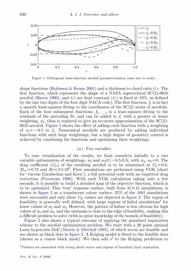
shape functions (Robinson & Keane 2001) and a thickness to chord ratio t/c. Thefirst function, which represents the shape of a NASA supercritical SC(2)-0610aerofoil (Harris 1990), and t/c are kept constant (t/c is fixed at 10%, as definedby the last two digits of the four digit NACA code). The first function, f1 is in facta smooth least-squares fitting to the coordinates of the SC(2) series of aerofoils.Each of the four subsequent functions, f2, ., 5 is a least-squares fitting to theresiduals of the preceding fit, and can be added to f1 with a greater or lesserweighting, wi , than is required to give an accurate approximation of the SC(2)-0610 aerofoil. Figure 1 shows the effect of adding each function with a weightingof wiZK0.5 to f1. Nonsensical aerofoils are produced by adding individualfunctions with such large weightings, but a high degree of geometry control isachieved by combining the functions and optimizing their weightings.

(a ) Two variables

To ease visualization of the results, we limit ourselves initially to a twovariable optimization of weightings, w2 and w32[K0.5,0.5], with w4, w5Z0. Thedrag coefficient (CD) of the resulting aerofoil is to be minimized at CLZ0.6,MNZ0.73 and ReZ3!106. Flow simulations are performed using VGK (shortfor ‘viscous Garabedian and Korn’), a full potential code with an empirical dragcorrection (Freestone 1996). With each VGK calculation taking only a fewseconds, it is possible to build a detailed map of the objective function, which isto be optimized. This ‘true’ response surface, built from 41!41 simulations, isshown in figure 2 as a translucent colour surface. 35% of the 1681 simulationswere successful and only these CD values are depicted in figure 2. The region offeasibility is generally well defined, with large regions of failed simulations4 forlower values of w2 and w3. However, the pattern of failure is less obvious for highvalues of w2 and w3, and the optimum is close to the edge of feasibility, making thisa difficult problem to solve (with no prior knowledge of the bounds of feasibility).

Figure 2 also shows a typical outcome of applying the penalized imputationscheme to the aerofoil optimization problem. We start with a 20 point optimalLatin hypercube DoE (Morris & Mitchell 1995), of which seven are feasible andare shown as black dots in figure 2. A Kriging model is fitted to the feasible data(shown as a coarse black mesh). We then add s2 to the Kriging prediction to

4 Failures are associated with strong shock waves and regions of boundary layer separation.


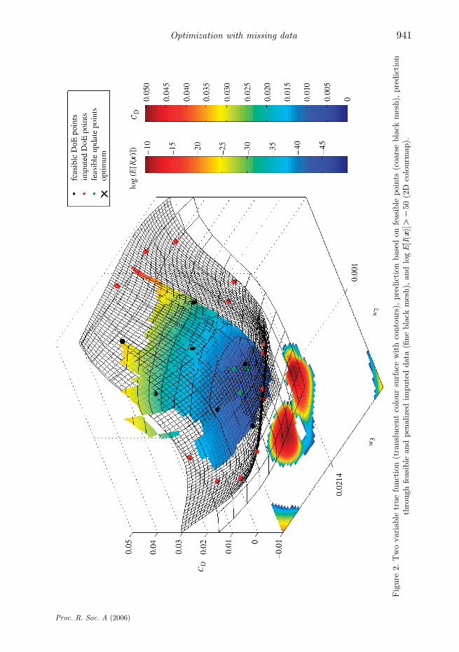
Figure

2.Twovariable

truefunction(translucentcoloursurface

withcontours),

predictionbasedonfeasible

points

(coarseblack

mesh),

prediction

throughfeasible

andpenalizedim

puteddata

(fineblack

mesh),

andlogE[I(x)]OK50(2D

colourm

ap).



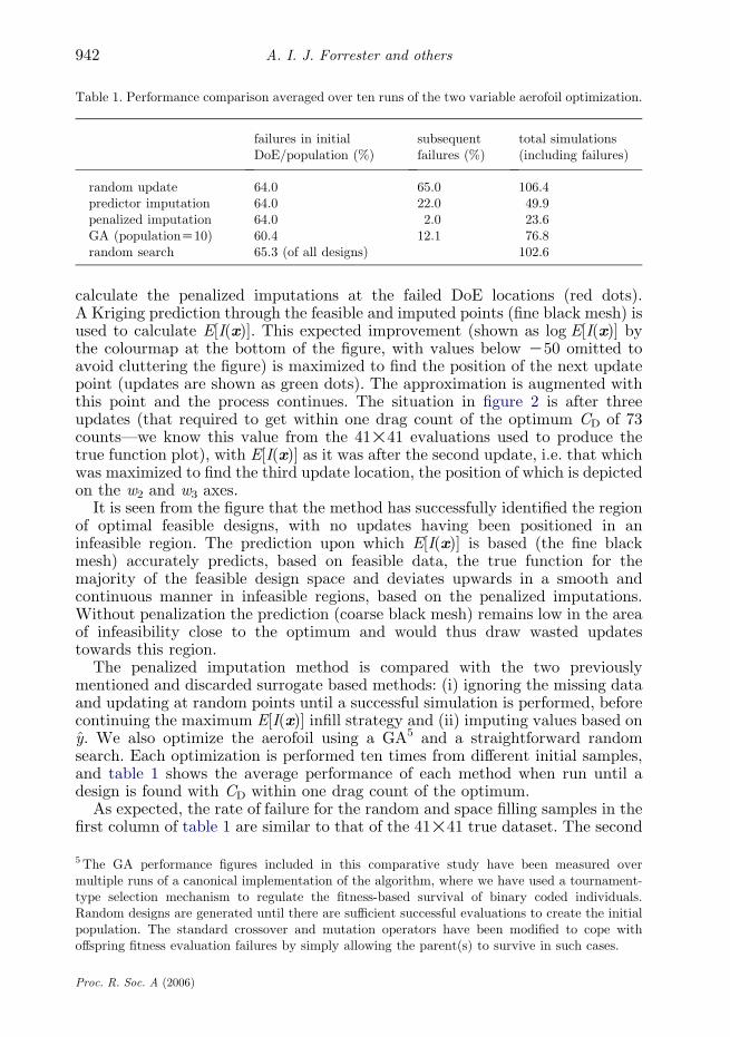
Table 1. Performance comparison averaged over ten runs of the two variable aerofoil optimization.

failures in initialDoE/population (%)

subsequentfailures (%)

total simulations(including failures)

random update 64.0 65.0 106.4predictor imputation 64.0 22.0 49.9penalized imputation 64.0 2.0 23.6GA (populationZ10) 60.4 12.1 76.8random search 65.3 (of all designs) 102.6


calculate the penalized imputations at the failed DoE locations (red dots).A Kriging prediction through the feasible and imputed points (fine black mesh) isused to calculate E[I(x)]. This expected improvement (shown as log E[I(x)] bythe colourmap at the bottom of the figure, with values below K50 omitted toavoid cluttering the figure) is maximized to find the position of the next updatepoint (updates are shown as green dots). The approximation is augmented withthis point and the process continues. The situation in figure 2 is after threeupdates (that required to get within one drag count of the optimum CD of 73counts—we know this value from the 41!41 evaluations used to produce thetrue function plot), with E[I(x)] as it was after the second update, i.e. that whichwas maximized to find the third update location, the position of which is depictedon the w2 and w3 axes.

It is seen from the figure that the method has successfully identified the regionof optimal feasible designs, with no updates having been positioned in aninfeasible region. The prediction upon which E[I(x)] is based (the fine blackmesh) accurately predicts, based on feasible data, the true function for themajority of the feasible design space and deviates upwards in a smooth andcontinuous manner in infeasible regions, based on the penalized imputations.Without penalization the prediction (coarse black mesh) remains low in the areaof infeasibility close to the optimum and would thus draw wasted updatestowards this region.

The penalized imputation method is compared with the two previouslymentioned and discarded surrogate based methods: (i) ignoring the missing dataand updating at random points until a successful simulation is performed, beforecontinuing the maximum E[I(x)] infill strategy and (ii) imputing values based ony. We also optimize the aerofoil using a GA5 and a straightforward randomsearch. Each optimization is performed ten times from different initial samples,and table 1 shows the average performance of each method when run until adesign is found with CD within one drag count of the optimum.

As expected, the rate of failure for the random and space filling samples in thefirst column of table 1 are similar to that of the 41!41 true dataset. The second

5 The GA performance figures included in this comparative study have been measured overmultiple runs of a canonical implementation of the algorithm, where we have used a tournament-type selection mechanism to regulate the fitness-based survival of binary coded individuals.Random designs are generated until there are sufficient successful evaluations to create the initialpopulation. The standard crossover and mutation operators have been modified to cope withoffspring fitness evaluation failures by simply allowing the parent(s) to survive in such cases.



column of update failures rates are more interesting. When missing data isignored a large number of updates are based on random sampling and thus thefailure rate is similar to the values in column one. When imputation is used thefailures drop dramatically, particularly when penalization forces the updatesaway from the infeasible region—just two per cent of designs failed here,corresponding to one design out of all ten optimization runs. With the initialpopulation of the GA concentrated within the feasible region, subsequent failuresare low here as well. As far as overall performance is concerned, ignoring themissing data proves to be no better than a random search. Although the GAdeals well with the missing data, such a search is more suited to finding optimalregions in higher dimensional or multi-modal problems and its final convergence toan accurate optimum is slow. The imputation based methods outperform the otheroptimizers, although the prediction imputation still wastes resources sampling ininfeasible regions, with penalized imputation proving to be over 50% faster.

(b ) Four variables

The problem is now extended to four variables, with w2, ., w52[K0.25,0.25].The region of feasibility can be visualized via the hierarchical axis plot in figure 3.The plot is built from 114 runs of the VGK code.6 Each tile shows CD for varyingw2 and w3 for a fixed w4 and w5. w4 and w5 vary from tile to tile with the value atthe lower left corner of each tile representing the value for the entire tile.

18% of the design space proved to be feasible, for which colour maps of the CD

are shown, with the colour scale the same as in figure 2. A large proportion of thedesign space is infeasible due to the simple reason of the upper and lower surfacesof the aerofoil intersecting at mid chord. Regions in which this occurs are shownin dark blue and the simplicity of the region means that it could be eliminated byadjusting the bounds of the variables. The blank areas in figure 3, however,indicate regions for which VGK has failed for designs where we cannot easilyidentify the geometry as being corrupt, e.g. extensive rippling of the aerofoilsurface produces problems with the convergence of flow simulations. Also,beyond the problem of identifying corrupt geometries, a sound geometry may faildue to its particular flow characteristics, e.g. the onset of stall before the CL

criterion is met. These factors combine to produce a complex domain offeasibility, which is awkward to identify. While efforts can be made to reduce thebounds of the problem to this feasible domain of interest, we cannot eliminatedesign evaluation failures completely without removing feasible designs and socompromising the global nature of the search.

The outcome of a run of the penalized imputation method using an initialoptimal Latin hypercube DoE of 200 points followed by 23 updates (again toattain a CD within one drag count of the optimum—now 70 counts) is shown infigure 3, with points depicted using the same legend as figure 2 (we display thebest run in order to produce a clearer figure with few points). Only discretevalues of w4 and w5 can be displayed and as such the design variables are roundedto the nearest 0.05 for the purpose of visualization. It should be borne in mindthat there is, in fact, a distribution of designs between tiles. The reader shouldalso appreciate that, although the major axis is much larger than the axes of the

6Generating such plots would, of course, not be possible in most cases due to the highcomputational cost. Here, we have computed this large quantity of data for illustrative purposes.


0 0.05 0.10 0.15 0.20 0.25

–0.05

–0.05–0.10–0.15–0.20

–0.10

–0.15

–0.20

–0.25

0

0.05

0.10

0.15

0.20

0.25

w4

w5

Figure 3. Four variable true function and penalized imputation method data points (see figure 2 forlegend). Red crosses indicate imputed update points. Regions of infeasible geometries are shown asdark blue.


individual tiles, they both represent the same variation across a variable. Thus,although there seems to be a wide distribution of update points across w4 and w5,these points represent a tight cluster in the region of optimal feasible designs.The initial approximation after the DoE was based on just 35 successful points,with the remaining 165 being imputed. Despite this small successful sample, it isseen that the feasible updates are clustered in optimal regions with only four ofthe updates having been positioned outside of the feasible region. Again we makecomparisons, averaged over five runs, with four other optimization methods intable 2.

Table 2 follows a similar pattern to table 1. We note here that the number offunction evaluations is relatively high for a four variable problem, due to theextremely large area of infeasibility coupled with the complexity of the noisy CD

landscape. Ignoring missing data has little impact on the failure rate, while it issignificantly reduced by using imputations. The GA performs best in these terms,but, as before, requires a large number of evaluations to reach the optimum.Aswell


Table 2. Performance comparison averaged over ten runs of the four variable aerofoil optimization.

failures in initialDoE/population (%)

subsequentfailures (%)

total simulations(including failures)

random update 81.7 77.5 774.6predictor imputation 81.7 40.8 bestZ421penalized imputation 81.7 36.2 308.8GA 80.6 21.8 874.4random search 80.0 (of all designs) 2316.8


as our CD%0.007 stopping criterion, we limit the number of points used to build asurrogate model to 500.7 Although when ignoring the missing data the size of theKriging model remains small, the total number of simulations is high. However,imputing values to thesemissing data increased the size of themodel, leading to thetermination of the prediction-based imputations for three out of the five runs priorto attaining the optimum CD and thus an averaged value is not available. Thebenefits of penalized imputations outweigh the increase in model size and, as in thetwo variable example, this method proves to be the most successful.

5. Conclusions

The use of imputation in regions of failure enables surrogate model based globaloptimization of unfamiliar design spaces. Such methods can provide significanttime savings over direct global search methods, such as GAs. The studiesperformed show promising results for the use of imputations penalized with astochastic process based statistical upper bound.

References

Freestone, M. M. 1996 VGK method for two-dimensional aerofoil sections. Technical Report96028, Engineering Sciences Data Unit, November 1996.

Harris, C. D. 1990 NASA supercritical airfoils—a matrix of family-related airfoils. NASA TechnicalPaper (2969), March 1990.

Jones, D. R. 2001 A taxonomy of global optimization methods based on response surfaces. J. GlobalOptim. 21, 345–383. (doi:10.1023/A:1012771025575)

Jones, D. R., Schlonlau, M. & Welch, W. J. 1998 Efficient global optimisation of expensive black-box functions. J. Global Optim. 13, 455–492. (doi:10.1023/A:1008306431147)

Little, R. J. A. & Rubin, D. B. 1987 Statistical analysis with missing data. New York: Wiley.Morris, M. D. & Mitchell, T. J. 1995 Exploratory designs for computer experiments. J. Stat. Plan.

Infer. 43, 381–402. (doi:10.1016/0378-3758(94)00035-T)Robinson, G. M. & Keane, A. J. 2001 Concise orthogonal representation of supercritical aerofoils.

J. Aircraft 38, 580–583.Sacks, J., Welch, W. J., Mitchell, T. J. & Wynn, H. 1989 Design and analysis of computer

experiments. Stat. Sci. 4, 409–423.Torn, A. & Zilinskas, A. 1987 Global optimization. Berlin: Springer.

7The size of the training sample limits the applicability of the technique. In our experience trainingthe Kriging model is prohibitively expensive beyond 500 points and/or 20 dimensions.


http://dx.doi.org/doi:10.1023/A:1012771025575

http://dx.doi.org/doi:10.1023/A:1008306431147

http://dx.doi.org/doi:10.1016/0378-3758(94)00035-T

optimization with missing data - university of southamptonaijf197/rspa20051608p.pdf · optimization...

Documents