– 1 –

Optimization using the NAG Library

The Numerical Algorithms Group

www.nag.com

1. Introduction

The NAG Library [1] is a collection of functions which encapsulates hundreds of

algorithms in mathematics and statistics, and which can be invoked by developers to

(efficiently and accurately) solve numerical problems in their applications. The use of

such a resource is intended to free developers from the obligation of writing (or

finding, or testing) implementations of such algorithms themselves, thereby enabling

them to devote more effort to other aspects of their application.

One of the fields covered by the Library is optimization, and this note is devoted to

the description of some of the ways in which the Library can be used to solve

problems in this area. We begin with a brief discussion (§2.1) of mathematical

optimization, and the way in which some optimization problems include constraints

(§2.2) on the solution. Determining the form of the problem (including any

constraints) is important because, as we shall see in §2.3, it is essential to use a solver

which is appropriate for the type of problem at hand; we illustrate this point in §2.4

with a simple example. Section 3 describes some of the functionality of the NAG

Library optimization solvers; we draw a distinction between local solvers (§3.1) and

global solvers (§3.2), before highlighting, in §3.3, the routines which have been added

to the Library in its latest release. We conclude §3 by looking at some related

problems which can be solved using routines from other chapters of the Library. Our

attention turns to applications of optimization in Section 4, which involves briefly

surveying (§4.1) a few examples from finance, manufacturing and business analytics

in which NAG solvers have been used before describing (§4.2) a specific financial

analysis application in more detail. A final section (§5) contains the conclusions of

this note.

– 2 –

2. Background

2.1 What is optimization?

Optimization is a wide-ranging and technically detailed subject, to which several

authoritative texts – for example, [2] [3] – have been devoted. It can be defined as

“the selection of a best element (with regard to some criteria) from some set of

available alternatives” [4]. Mathematically, it consists of locating the maximum or

minimum of a function of variables (called the objective function):

( )

( )

( )

(1)

That is, we seek the values for which correspond to a maximum or

minimum value for . Since maximizing ( ) is equivalent to minimizing the

negative of ( ), we can without loss of generality consider minimization only from

hereon.

A distinction may immediately be drawn between finding a local minimum –

where, for all near , ( ) ( ) – and a global minimum, where this condition

is fulfilled for all . We note that there is a large class of optimization problems [5]

which have at most one local minimum – that is, there is no difference between the

two types of minimum. Whilst many algorithms have been developed for local

optimization, the development of reliable methods for global optimization (especially

for large-scale problems) has been harder to do. It should also be noted that

circumstances often arise where the determination of a local minimum is sufficient for

the user – for example, for problems in which application of global optimization

methods are intractable, or less reliable than local methods, or if the user possesses

other information about a desired local minimum.

Methods for optimization often require information related to the derivatives of the

objective function, in order to assist with the search for the minimum. More

specifically, the elements of the gradient vector (the vector of first derivatives of

with respect to each of the ) and the Hessian matrix (the square matrix of second

derivatives of ) are defined as:

– 3 –

( )

( )

(2)

A simple illustration of the use of derivatives in optimization can be found in §2.3, in

the description of the so-called steepest descent method, which uses explicitly – see

equation (10).

2.2 Constraining the problem

Many optimization problems are unconstrained – that is, there are no restrictions on

the values that the solution vector may take. Other problems are supplemented by

such restrictions – for example, in a demographic study, a population cannot be

negative. These are usually specified by a set of constraint functions, for example:

(3)

which are bound constraints, or

(4)

which is an example of a linear constraint, or

(5)

which is a non-linear constraint. The three types of constraint can be expressed

succinctly as

{

( )

} (6)

in which and are vectors of lower and upper bound values, is a constant matrix,

and is a vector of nonlinear constraint functions.

– 4 –

2.3 Using the appropriate solver

A single, all-purpose optimization method does not currently exist. Instead, different

methods have been developed (and which are offered by NAG) that are suitable for

particular forms of optimization problem. Using a method that is inappropriate for the

problem at hand can be cumbersome and/or inefficient and, whilst it is always

possible to use a method which is more generic than necessary, it will usually be

massively outperformed by specialized solvers which are aimed at specific forms of

problem.

The form of the optimization problem is determined by the properties of the objective

function, and by the form of the constraints (if any). More specifically, a distinction

is made between objective functions that are linear, quadratic and nonlinear.

Another distinction may be made if the objective function can be written as

( ) ∑

( ) (7)

in which case the optimization is referred to as a least squares problem (which may be

further classified as nonlinear or linear, depending on the form of the functions ).

Some specific combinations of the properties of the objective function and the

constraints receive special designation; thus, linear constraints together with a linear

is referred to as a linear programming (LP) problem; linear constraints plus a

quadratic makes a quadratic programming (QP) problem, whilst any type of

constraints with a nonlinear is called a nonlinear programming (NLP) problem.

2.4 An example problem

We illustrate the way in which different solution methods can perform in different

ways for the same problem in Figure 1, which shows two attempts to find the

minimum of the so-called Rosenbrock function [6]:

( ) ( ) (

) (8)

This is a function which was designed as a performance test for optimization

algorithms. It has a global minimum at

– 5 –

( ) (9)

which is within a long, narrow, parabolic-shaped flat valley. The two methods used in

Figure 1 to minimize (8) are called steepest (or gradient) descent [7], and a sequential

quadratic programming (SQP) method [3], as implemented in the NAG Library [8].

The former is easier to understand (and program) than the latter: specifically, at each

point, the method takes a step in the direction of the negative gradient at that point:

( ) ( ) ( ) ( ( )) (10)

where ( ), the step size at the -th step, is proportional to | ( ( ))|, the modulus of

Figure 1. Finding the minimum of Rosenbrock's function in

MATLAB® using the method of steepest descent (top) and a method

from the NAG Library (bottom).

– 6 –

the gradient at that step. Figure 1 shows that, whilst this method is able to find the

location of the valley in a few big steps, its progress along the valley takes many more

small steps, because of the link between the size of the step and the gradient. The

method terminates after 400 steps in this example, with the current step still being a

long way away from the minimum. By contrast, the SQP method converges to the

minimum in 55 steps. (The number of steps taken by an optimization method should

be as small as possible for efficiency’s sake, because it is proportional to the number

of times the objective function is evaluated, which can be computationally expensive.)

We recall that many optimization methods require information about the objective

function’s derivatives. The NAG implementation of the SQP method has an option

for these to be specified explicitly (in the same way that the form of the objective

function is described); otherwise, it approximates the derivatives using finite

difference methods1. This clearly requires many more evaluations of the objective

function – to be specific, in this example, it increases the number of steps required for

convergence to 280.

Similar conclusions about efficiency and the provision of derivative information could

be reached by examining the performance for the solution of a given problem of – for

example – three NAG implementations of a modified Newton method [9]; one which

uses function values only [10], one which also uses first derivatives [11], and one

which also uses first and second derivatives [12].

Finally in this section, we note that the Rosenbrock function (8) can be written in the

form of (7), which turns its minimization into a non-linear least squares problem:

( ) ( )

( )

( ) ( )

( ) ( )

(11)

Switching to a quasi-Newton method [13] which is specially designed for this type of

problem – implemented in the NAG Library at [14] – results in a convergence to the

1 Other NAG functions bypass the requirement for gradients by using specialized optimization methods

such as BOBYQA [26] or Nelder-Mead [28] which do not require derivatives to determine the next

step in the optimization sequence – see §3.3, below.

– 7 –

minimum in 19 steps (which, since this method requires specification of derivatives,

is to be compared with the 55 steps required by the more general SQP method when

derivatives are provided).

3. Optimization and the NAG Library

In this section we look at the range of functionality and applicability that the NAG

Library offers for optimization problems. We consider both local (§3.1) and global

(§3.2) optimization and, whilst we do not for the most part discuss individual routines

in detail, describe in §3.3 the enhancements in optimization functionality which have

been included [15] in the most recent release (Mark 23) of the NAG Library. Finally

in this section, we mention (§3.4) a few optimization problems that can be solved

using functions from non-optimization chapters in the Library.

We note in passing that the functions in the Library can be accessed from a variety of

computing environments and languages [16] including MATLAB and Microsoft

Excel (see figures 1-3 for examples). In addition, some work has been recently done

[17] to build interfaces between NAG solvers and AMPL, a specialized language

which is used for describing optimization problems. Interfaces to two NAG solvers

are described in detail (and are available for download from the NAG website), which

provides a useful starting point for the development of AMPL interfaces to other

routines, and the construction of mechanisms for calling NAG routines from other

optimization environments.

3.1 Local optimization

The NAG Library contains a number of routines for the local optimization of linear,

quadratic or nonlinear objective functions; of objective functions that are sums of

squares of linear or nonlinear functions; subject to bounded, linear, sparse linear,

nonlinear or no constraints. The documentation of the local optimization chapter [18]

describes how to choose the most appropriate routine for the problem at hand with the

help of a decision tree which incorporates questions such as:

What kind of constraints does the problem have?

o None

o Bound

o Linear

– 8 –

If so, is the matrix of linear constraints [see (6)] sparse?

o Nonlinear

What kind of form does the objective function have?

o Linear

o Quadratic

o Sum of squares

o Nonlinear

Does the objective function have one variable?

Are first derivatives available?

o If so, are second derivatives available?

Is computational cost critical?

Is storage critical?

Are you an experienced user?

The last question is related to the fact that many of the optimization methods are

implemented in two routines: namely, a comprehensive form and an easy-to-use form.

The latter are more appropriate for less experienced users, since they include only

those parameters which are essential to the definition of the problem (as opposed to

parameters relevant to the solution method). The comprehensive routines use

additional parameters which allow the user to improve the method’s efficiency by

‘tuning’ it to a particular problem.

3.2 Global optimization

The Library contains implementations of three methods for the solution of global

optimization problems. As previously (§3.1), the documentation for this chapter [19]

provides the user with suggestions about the choice of the most appropriate routine for

the problem at hand.

nag_glopt_bnd_mcs_solve [20] uses a multilevel coordinate search

[21] which recursively splits the search space (i.e. that within which the

minimum is being sought) into smaller subspaces in a non-uniform fashion.

The problem may be unconstrained, or subject to bound constraints. The

routine does not require derivative information, but the objective function

must be continuous in the neighbourhood of the minimum, otherwise the

method is not guaranteed to converge. The use of this routine is illustrated in

– 9 –

Figure 2, the upper part of which shows a demo function having more than one

minimum2. The workings of the method are shown in the bottom part of the

2 More specifically, this is MATLAB’s peaks function.

Figure 2. Globally optimizing a function with more than one minimum (displayed as

a surface at top) using a method from the NAG Library (bottom).

– 10 –

figure, which displays the function as a contour plot, along with the search

subspaces and objective function evaluation points chosen by the method; it

can be seen that – for this example – the method spends most of its time in and

around the two minima, before correctly identifying the global minimum as

the lower of the two.

nag_glopt_nlp_pso [22] uses a stochastic method based on particle

swarm optimization [23] to search for the global minimum of the objective

function. The problem may be unconstrained, or subject to bound, or linear, or

nonlinear constraints (there also exists a simpler variant [24] of the routine

which only handles bound – or no – constraints). The routine does not require

derivative information, although this could be used by the optional

accompanying local optimizers. A particular feature of this routine is that it

can exploit parallel hardware, since it allows multiple threads to advance

subiterations of the algorithm in an asynchronous fashion.

nag_glopt_nlp_multistart_sqp [25] finds the global minimum of an

arbitrary smooth function subject to constraints (which may include simple

bounds on the variables, linear constraints and smooth nonlinear constraints)

by generating a number of different starting points and performing a local

search from each using SQP. This method can also exploit parallel hardware,

in the same fashion as the particle swarm method.

3.3 Recent additions to NAG Library optimization functionality

Two of the global optimization routines described in §3.2 (specifically,

nag_glopt_nlp_pso and nag_glopt_nlp_multistart_sqp) are new in

the most recent release of the NAG Library. In addition, the following local

optimization routines were also added to the Library at that release:

nag_opt_bounds_qa_no_deriv [26] is an easy-to-use routine that uses

methods of quadratic approximation to find a local minimum of an objective

function ( ), subject to bound constraints on the . It is useful for problems

where the computation of derivatives of is either impossible or numerically

intractable – for example, if is the result of a simulation. The routine uses

the BOBYQA (Bound Optimization BY Quadratic Approximation) algorithm

– 11 –

[27] whose efficiency is preserved for large problem sizes3. For example, it

solves the problem of distributing 50 points on a sphere to have maximal

pairwise separation (starting from equally spaced points on the equator) using

4633 evaluations of . This is to be compared with, for example, the NAG

routine [28] which uses the so-called Nelder-Mead simplex solver [29] and

takes 16757 evaluations.

nag_opt_nlp_revcomm [30] is designed to locally minimize an arbitrary

smooth function subject to constraints (which may include simple bounds,

linear constraints and smooth nonlinear constraints) using an SQP method.

The user should supply as many first derivatives as possible; any unspecified

derivatives are approximated by finite differences. It may also be used for

unconstrained, bound-constrained and linearly-constrained optimization. It

uses a similar algorithm to nag_opt_nlp [31], but has an alternative

interface4.

3.4 Solving optimization problems using other NAG routines

In addition to the standard types of optimization problem which the routines from the

two optimization chapters [18] [19] can be used to solve, there are a few related

problems that can be solved using functions in other chapters of the NAG Library.

For example, there are several routines in the Least Squares and Eigenvalue Problems

chapter of the Library [32] which perform the minimization of

( ) ∑ ( )

(12)

where the residual is defined as

3 i.e., large in equation (1).

4 Specifically, it uses so-called reverse communication [55], as opposed to forward communication

which requires that user-supplied procedures – such as that which calculates ( ) – be included in the

function argument list, so that they can be called from the routine. Opting for the reverse

communication interface – which is used in many NAG Library routines – is helpful when it is

impractical or inconvenient to pass user’s data into callback routines, or when interfacing with

complicated environments.

– 12 –

( ) ∑

(13)

In a similar fashion, the minimization of other metrics – for example the so-called

norm [33]

( ) ∑| ( )|

(14)

or the norm,

( )

| ( )| (15)

can be solved5 using routines from the curve and surface fitting chapter of the Library.

Finally in this section, we mention a NAG routine [34] which solves various types of

integer programming problem. Briefly, these are LP and QP problems – possibly

incorporating linear constraints (6) – where some (or all) of the elements of the

solution vector are restricted to taking either only integer values, or only zero or

one. The routine uses a branch and bound method that divides the problem up into

sub-problems, each of which is solved internally using a QP solver from the local

optimization chapter [35].

4. Applications

Optimization is a technique which has been used in the solution of many problems

from a wide variety of domains. These range [4] from engineering (rigid body

dynamics, design optimization, control engineering) and operations research

(scheduling, routing, critical path analysis) to economics (expenditure minimization

problems and trade theory). Solutions to other – more abstract – optimization

problems, such as mesh smoothing, shape optimization or particle steering can be

useful in multiple domains.

A complete review of optimization applications is beyond the scope of this section;

instead we first describe (§4.1) a few examples of interest where NAG optimization

routines have been used, before focusing (§4.2) on a simple problem taken from

finance – namely, portfolio optimization – and presenting a reasonably detailed

5 nag_lone_fit [57] for the norm, or nag_linf_fit [56] for the norm.

– 13 –

description of the way in which NAG functions can be used to solve it; this also

serves to highlight how they can be invoked from within various environments by

users with little or no programming knowledge.

We note in passing that use of the NAG Library for portfolio optimization has

previously been discussed elsewhere [36]. Our account in §4.2 is less comprehensive,

but takes more recent developments – including the Library interfaces with MATLAB

and Microsoft Excel, and the treatment of the nearest correlation matrix [37] – into

account. The interested reader is referred to [36] for a more detailed and authoritative

account of this subject.

4.1 Optimization examples using NAG

Examples of applications which use NAG routines for optimization include index

tracking [38]. This problem – which is related to portfolio optimization (§4.2) – aims

to replicate the movements of the index of a particular financial market, regardless of

changes in market conditions, and can also be tackled using optimization methods. In

fact, the same NAG method [39] that is used for the portfolio optimization problem

can also be used here.

Optimization is also heavily used in the calibration of derivative pricing models [40],

in which values for the parameters of the model are calculated by determining the best

match between the results of the model and historical prices (known as the calibration

instruments). This can be expressed as the minimization of, for example, the chi-

squared metric:

∑

( ) (16)

i.e., the weighted sum, over the instruments in the calibration set, of the difference

between the market price of instrument and its price ( ) as predicted by the

model for some set of parameters . The weight is used to reflect the confidence

with which the market price for is known. As noted above (§3.4), it is also possible

to use other metrics – such as the (weighted) and norms – here. The

optimization problem is then how to determine the which minimizes the metric.

Other users [41] have optimized the performance of power stations by developing

mathematical models of engineering processes, and using NAG optimization routines

– 14 –

to solve them. The same routines have also found application in the solution of shape

optimization problems in manufacturing and engineering [42].

In the field of business analytics, NAG optimization routines have been used [43] in

the development of applications to help customers with – for example – fitting to a

pricing model used in the planning of promotions, and maximizing product income by

combining its specification, distribution channel and promotional tactics.

Other applications include the use of optimization for parameter estimation in the

fitting of statistical models to observed data [44].

4.2 Portfolio optimization

Portfolio optimization addresses the question of diversification – that is, how to

combine different assets in a portfolio which achieves maximum return with minimal

risk. This problem was initially addressed by Markowitz [45]; we outline its

treatment here.

We assume that the portfolio contains assets, each of which has a return . Then,

the return from the portfolio is

( ) ∑

(17)

where is the proportion of the portfolio invested in asset . We further assume that

each is normally distributed with mean and variance ; the vector of returns

then has ( ) distribution, with the vector of means and the covariance

matrix. These can be, for example, calculated from historical data:

∑ ( )

∑ ( ) ( )

(18)

for a collection of observations of at times (we note in passing that the NAG

Library contains a routine [46] for calculating and , as well as other statistical

data).

The expectation and variance of the portfolio return are

– 15 –

( ) ∑

( ) ∑∑

(19)

The portfolio optimization problem is then to determine the which results in a

specific return , with minimum risk. We define the latter as the variance of the

return – see (19). The objective function is then ( ) – i.e., the optimization

problem can then be stated as

(20)

with the constraint

∑

(21)

This problem can be solved using a QP method [47], as implemented in the NAG

Library at [39]. The problem may incorporate constraints – for example, that the

whole portfolio be fully invested:

∑

(22)

In addition, the composition of the portfolio may be constrained across financial

sectors. For example, the requirement that up to 20% be invested in commodities, and

at least 10% in emerging markets may be specified as

∑

∑

(23)

where each element of the coefficient vectors and is either 0 or 1, depending on

the classification of asset . Other types of linear constraints might capture the

– 16 –

selection of assets based on geography or stock momentum, while simple bound

constraints of the form of (3) can be used to allow or prohibit shorting6.

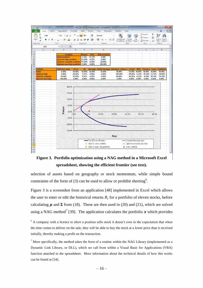
Figure 3 is a screenshot from an application [48] implemented in Excel which allows

the user to enter or edit the historical returns for a portfolio of eleven stocks, before

calculating and from (18). These are then used in (20) and (21), which are solved

using a NAG method7 [39]. The application calculates the portfolio which provides

6 A company with a licence to short a position sells stock it doesn’t own in the expectation that when

the time comes to deliver on the sale, they will be able to buy the stock at a lower price than it received

initially, thereby making a profit on the transaction.

7 More specifically, the method takes the form of a routine within the NAG Library (implemented as a

Dynamic Link Library, or DLL), which we call from within a Visual Basic for Applications (VBA)

function attached to the spreadsheet. More information about the technical details of how this works

can be found at [54].

Figure 3. Portfolio optimization using a NAG method in a Microsoft Excel

spreadsheet, showing the efficient frontier (see text).

– 17 –

a return (entered by the user), at minimum risk. It also calculates the so-called

efficient frontier [49], which shows the highest expected return for each level of risk.

The simplicity of this portfolio model is helpful for the purposes of explication and

the construction of a demo application but, as is well-known [45], it suffers from a

number of drawbacks that impede its application to real-world problems. For

example, the assumption that the returns are normally distributed is not borne out in

practice, nor is it the case that correlations between assets do not change in time8. It

also assumes that over-performance (a return greater than ) is to be eschewed in the

same way as under-performance; such an equal weighting clearly does not correspond

to the desires of real investors. In practice, quantitative analysts use models that are

more sophisticated than that described here – see, for example, the work described in

[50] – which in turn require the use of a more general optimizer from the NAG

Library.

Before leaving this subject, we mention a related area where NAG methods are

proving helpful. The treatment above – and also that of more sophisticated models –

requires that the matrix is positive semi-definite – i.e., that the quantity is non-

negative for all (this is part of the definition of a covariance matrix, and is a

requirement for the optimizer to work). In practice, this is often not the case, since

is calculated from historical data [see (18)], which might be incomplete, thus

rendering invalid for use here. A method which determines , the nearest positive

semi-definite matrix to , by minimizing their Frobenius separation has been recently

developed [51] [52], and has been implemented in the NAG Library [37]. Having

calculated in this fashion, it can then be used in (20) in place of .

5. Conclusions

In this note, we have examined some characteristics of optimization problems,

including their categorization, and the importance of using an appropriate solver for

the type of problem at hand. In this context, we have described some of the solvers

which can be found in the optimization chapters of the NAG Library, together with

other NAG routines that can be applied to the solution of optimization problems. We

8 For example, during a financial crisis, all assets tend to become positively correlated, because they all

move in the same direction (i.e. down).

– 18 –

have also briefly reviewed a few example applications which have incorporated the

use of NAG solvers.

Readers who are interested in finding out more about NAG’s optimization

functionality, or who require advice on its application to specific problems, are

encouraged to contact our optimization specialists via the NAG helpdesk.

Finally, it should perhaps be mentioned that, along with the routines that have been

mentioned in this note, the NAG Library [1] contains user-callable routines for

treatment of a wide variety of numerical and statistical problems, including – for

example – linear algebra, statistical analysis, quadrature, correlation and regression

analysis and random number generation.

6. Acknowledgements

We thank Jeremy Walton for writing this note and other colleagues David Sayers,

Martyn Byng, Jan Fiala, Marcin Krzysztofik and Mick Pont for many helpful

technical discussions during preparation.

7. Bibliography

1. Numerical Algorithms Group. NAG numerical components. [Online]

http://www.nag.com/numeric/numerical_libraries.asp.

2. Gill, P.E. and Murray, W., [ed.]. Numerical Methods for Constrained

Optimization. London : Academic Press, 1974.

3. Fletcher, R. Practical Methods of Optimization. 2nd edn. Chichester : Wiley, 1987.

4. Wikipedia. Mathematical optimization. [Online]

http://en.wikipedia.org/wiki/Mathematical_optimization.

5. —. Convex optimization. [Online]

http://en.wikipedia.org/wiki/Convex_optimization.

6. —. Rosenbrock function. [Online]

http://en.wikipedia.org/wiki/Rosenbrock_function.

7. —. Gradient descent. [Online] http://en.wikipedia.org/wiki/Gradient_descent.

8. Numerical Algorithms Group. nag_opt_nlp_solve (e04wd) routine document.

[Online] http://www.nag.co.uk/numeric/CL/nagdoc_cl23/pdf/E04/e04wdc.pdf.

– 19 –

9. Gill, P.E. and Murray, W. Minimization subject to bounds on the variables.

National Physical Laboratory. 1976. NPL Report NAC 72.

10. Numerical Algorithms Group. nagf_opt_bounds_quasi_func_easy (e04jy)

routine document. [Online]

http://www.nag.co.uk/numeric/fl/nagdoc_fl23/pdf/E04/e04jyf.pdf.

11. —. nagf_opt_bounds_quasi_deriv_easy (e04ky) routine document. [Online]

http://www.nag.co.uk/numeric/fl/nagdoc_fl23/pdf/E04/e04kyf.pdf.

12. —. nagf_opt_bounds_mod_deriv2_easy (e04ly) routine document. [Online]

http://www.nag.co.uk/numeric/fl/nagdoc_fl23/pdf/E04/e04lyf.pdf.

13. Algorithms for the solution of the nonlinear least-squares problem. Gill, P.E. and

Murray, W. 1978, SIAM J. Numer. Anal., Vol. 15, pp. 977-992.

14. Numerical Algorithms Group. nag_opt_lsq_deriv (e04gb) routine document.

[Online] http://www.nag.co.uk/numeric/CL/nagdoc_cl23/pdf/E04/e04gbc.pdf.

15. —. NAG C Library News, Mark 23. [Online]

http://www.nag.co.uk/numeric/CL/nagdoc_cl23/pdf/GENINT/news.pdf.

16. —. Languages and Environments. [Online] http://www.nag.co.uk/languages-and-

environments.

17. Fiala, Jan. Nonlinear Optimization Made Easier with the AMPL Modelling

Language and NAG Solvers. [Online]

http://www.nag.co.uk/NAGNews/NAGNews_Issue95.asp#Article1.

18. Numerical Algorithms Group. NAG Chapter Introduction: e04 - Minimizing or

Maximizing a Function. [Online]

http://www.nag.co.uk/numeric/CL/nagdoc_cl23/pdf/E04/e04intro.pdf.

19. —. NAG Chapter Introduction: e05 - Global Optimization of a Function . [Online]

http://www.nag.co.uk/numeric/CL/nagdoc_cl23/html/E05/e05intro.html.

20. —. nag_glopt_bnd_mcs_solve (e05jb) routine document. [Online]

http://www.nag.co.uk/numeric/CL/nagdoc_cl23/pdf/E05/e05jbc.pdf.

21. Global optimization by multi-level coordinate search. Huyer, W. and Neumaier,

A. 1999, Journal of Global Optimization, Vol. 14, pp. 331-355.

– 20 –

22. Numerical Algorithms Group. nag_glopt_nlp_pso (e05sb) routine document.

[Online] http://www.nag.co.uk/numeric/CL/nagdoc_cl23/pdf/E05/e05sbc.pdf.

23. Vaz, A.I. and Vicente, L.N. A Particle Swarm Pattern Search Method for Bound

Constrained Global Optimization. Journal of Global Optimization. Vol. 39, 2, pp.

197-219.

24. Numerical Algorithms Group. nag_glopt_bnd_pso (e05sa) routine document.

[Online] http://www.nag.co.uk/numeric/CL/nagdoc_cl23/pdf/E05/e05sac.pdf.

25. —. nag_glopt_nlp_multistart_sqp (e05uc) routine document. [Online]

http://www.nag.co.uk/numeric/CL/nagdoc_cl23/html/E05/e05ucc.html.

26. —. nag_opt_bounds_qa_no_deriv (e04jc) function document. [Online]

http://www.nag.co.uk/numeric/CL/nagdoc_cl23/pdf/E04/e04jcc.pdf.

27. Powell, M.J.D. The BOBYQA algorithm for bound constrained optimization

without derivatives. University of Cambridge. 2009. Report DAMTP 2009/NA06.

28. Numerical Algorithms Group. nag_opt_simplex_easy (e04cb) function

document. [Online]

http://www.nag.co.uk/numeric/CL/nagdoc_cl23/pdf/E04/e04cbc.pdf.

29. A simplex method for function minimization. Nelder, J.A. and Mead, R. 1965,

Comput. J., Vol. 7, pp. 308–313.

30. Numerical Algorithms Group. nag_opt_nlp_revcomm (e04uf) function

document. [Online]

http://www.nag.co.uk/numeric/CL/nagdoc_cl23/pdf/E04/e04ufc.pdf.

31. —. nag_opt_nlp (e04uc) function document. [Online]

http://www.nag.co.uk/numeric/CL/nagdoc_cl23/pdf/E04/e04ucc.pdf.

32. —. NAG chapter introduction - f08: Least Squares and Eigenvalue Problems.

[Online] http://www.nag.co.uk/numeric/CL/nagdoc_cl23/pdf/F08/f08intro.pdf.

33. Wikipedia. Norm (mathematics). [Online]

http://en.wikipedia.org/wiki/Norm_(mathematics).

34. Numerical Algorithms Group. nag_ip_bb (h02bb) routine document. [Online]

http://www.nag.co.uk/numeric/CL/nagdoc_cl23/pdf/H/h02bbc.pdf.

– 21 –

35. —. nag_opt_qp (e04nf) routine document. [Online]

http://www.nag.co.uk/numeric/CL/nagdoc_cl23/pdf/E04/e04nfc.pdf.

36. Fernando, K.V. Practical Portfolio Optimization. [Online]

http://www.nag.co.uk/doc/techrep/index.html#np3484.

37. Numerical Algorithms Group. nag_nearest_correlation (g02aa) routine

document. [Online]

http://www.nag.co.uk/numeric/CL/nagdoc_cl23/pdf/G02/g02aac.pdf.

38. Wikipedia. Index fund. [Online] http://en.wikipedia.org/wiki/Index_fund.

39. Numerical Algorithms Group. nag_opt_lin_lsq (e04nc) routine document.

[Online] http://www.nag.co.uk/numeric/CL/nagdoc_cl23/pdf/E04/e04ncc.pdf.

40. Wikipedia. Derivative pricing. [Online]

http://en.wikipedia.org/wiki/Mathematical_finance.

41. Numerical Algorithms Group. PowerGen optimises power plant performance

using NAG's Algorithms. [Online]

http://www.nag.co.uk/Market/articles/NLCS213.asp.

42. Stebel, J. Test of numerical minimization package for the shape optimization of a

paper making machine header. [Online]

http://www.nag.co.uk/IndustryArticles/janstebel.pdf.

43. Walton, Jeremy, Fiala, Jan and Kubat, Ken. Case Study: Optimization for a

client with large-scale constrained problems. [Online]

http://www.nag.co.uk/Market/optimization_large-scale_constrained_problems.pdf.

44. Morgan, Geoff. The Use of NAG Optimisation Routines for Parameter

Estimation. [Online]

http://www.nag.co.uk/IndustryArticles/OptimisationParameterEstimation.pdf.

45. Wikipedia. Modern Portfolio Theory. [Online]

http://en.wikipedia.org/wiki/Portfolio_theory.

46. Numerical Algorithms Group. nag_corr_cov (g02bx) routine document.

[Online] http://www.nag.co.uk/numeric/CL/nagdoc_cl23/pdf/G02/g02bxc.pdf.

47. Gill, P.E., et al. Users’ guide for LSSOL (Version 1.0) Report SOL 86-1.

Department of Operations Research, Stanford University. 1986.

– 22 –

48. Numerical Algorithms Group. Demo Excel spreadsheet using NAG method to

solve portfolio optimization problem. [Online]

http://www.nag.co.uk/numeric/NAGExcelExamples/Portf_Opt_Simple_demo_FLDL

L.xls.

49. Wikipedia. Efficient Frontier. [Online]

http://en.wikipedia.org/wiki/Efficient_frontier.

50. Numerical Algorithms Group. Morningstar use NAG Library routines to assist

portfolio construction and optimization. [Online]

http://www.nag.co.uk/Market/articles/morningstar.pdf.

51. A quadratically convergent Newton method for computing the nearest correlation

matrix. Qi, J. and Sun, D. 2, 2006, SIAM J. Matrix Anal. Appl., Vol. 29, pp. 360-

385.

52. A preconditioned (Newton) algorithm for the nearest correlation matrix.

Borsdorf, R. and Higham, N.J. 1, 2010, IMA Journal of Numerical Analysis, Vol.

30, pp. 94-107.

53. SNOPT: An SQP Algorithm for Large-scale Constrained Optimization. Gill, P.E.,

Murray, W. and Saunders, M.A. 2002, SIAM J. Optim., Vol. 12, pp. 979-1006.

54. Krzysztofik, Marcin and Walton, Jeremy. Using the NAG Library to calculate

financial option prices in Excel. [Online]

http://www.nag.co.uk/IndustryArticles/NAGOptionPricingExcel.pdf.

55. Krzysztofik, Marcin. Reverse Communication in the NAG Library explained.

[Online] http://www.nag.co.uk/NAGNews/NAGNews_Issue95.asp#Article2.

56. Numerical Algorithms Group. nag_linf_fit (e02gc) routine document. [Online]

http://www.nag.co.uk/numeric/CL/nagdoc_cl23/pdf/E02/e02gcc.pdf.

57. —. nag_lone_fit (e02ga) routine document. [Online]

http://www.nag.co.uk/numeric/CL/nagdoc_cl23/pdf/E02/e02gac.pdf.

58. —. nag_opt_nlp_sparse (e04ug) routine document. [Online]

http://www.nag.co.uk/numeric/CL/nagdoc_cl23/pdf/E04/e04ugc.pdf.