optimization techniques for the dimensioning and ... of mpls networks sergio ariel beker to cite...
TRANSCRIPT

HAL Id: pastel-00000689https://pastel.archives-ouvertes.fr/pastel-00000689
Submitted on 6 Sep 2004
HAL is a multi-disciplinary open accessarchive for the deposit and dissemination of sci-entific research documents, whether they are pub-lished or not. The documents may come fromteaching and research institutions in France orabroad, or from public or private research centers.
L’archive ouverte pluridisciplinaire HAL, estdestinée au dépôt et à la diffusion de documentsscientifiques de niveau recherche, publiés ou non,émanant des établissements d’enseignement et derecherche français ou étrangers, des laboratoirespublics ou privés.
Optimization Techniques for the Dimensioning andReconfiguration of MPLS Networks
Sergio Ariel Beker
To cite this version:Sergio Ariel Beker. Optimization Techniques for the Dimensioning and Reconfiguration of MPLSNetworks. domain_other. Télécom ParisTech, 2004. English. �pastel-00000689�
These
presentee pour obtenir le grade de docteur
de l’Ecole Nationale Superieure des Telecommunications
Specialite : Informatique et Reseaux
Sergio BEKER
Techniques d’Optimisation pour le Dimensionnement et laReconfiguration des Reseaux MPLS
soutenue le 5 avril 2004 devant le jury compose de
Roberto Sabella (CORITEL) President
Walid BenAmeur (INT)
Deep Medhi (UMKC) Rapporteurs
Eitan Altman (INRIA)
Renaud Moignard (FTR&D) Examinateurs
Daniel Kofman (Telecom Paris) Directeur de these
Contact: Sergio Beker <[email protected]>


A Pascale...


Resume
La superposition de topologies virtuelles a la topologie physique d’un reseau est un desprincipaux mecanismes de l’ingenierie de trafic. Soit un reseau physique d’une certainetopologie et capacite fixees et une matrice de trafic a vehiculer, il s’agit de trouver unetopologie logique permettant de mapper de maniere optimale la matrice de trafic sur lereseau physique. A titre d’exemple, la topologie logique peut etre batie grace a des connex-ions ATM ou MPLS; c’est d’ailleurs une des principales raisons de l’interet qui est porte denos jours sur MPLS.
Cette gestion centralisee des ressources peut etre vue comme une generalisation du partagede charge, prenant en compte une vision globale du reseau au lie de se limiter a l’ensembledes chemins entre deux points. Mais les deux outils peuvent etre vus comme complemen-taires si on les regarde a differentes echelles de temps. En effet, changer un layout s’avereplus complique que changer une politique de partage de charge. Lors de l’evolution de lamatrice de trafic, on peut imaginer qu’on fasse evoluer les politiques de partage de chargeafin de pouvoir maintenir le niveau de QoS attendu sans avoir a modifier le layout. Il estclair que sur des echelles de temps plus longues et donc face a des variations importantesde la matrice de trafic, il faudra agir sur le layout.
Nos travaux dans ce domaine ont ete realises dans le contexte du projet RNRT VTHDet VTHD++. Nous avons apporte deux contributions principales. La premiere concernela definition de fonctions de cout que nous considerons mieux adaptees a la realite d’unoperateur que celles utilisees habituellement, la deuxieme concerne la prise en compte ducout de changement d’un layout. Les fonctions de cout usuellement utilisees visent a min-imiser certaines metriques telles que le delai. Nous ne considerons que cela soit une bonneapproche. A partir d’un certain seuil les applications deviennent insensibles a une reduc-tion supplementaire du delai de traversee du reseau. Le delai maximum est une contrainteque l’on doit repecter. Il est par contre interessant d’un point de vu operateur de reduireles couts d’operation et maintenance et donc, en particulier, de reduire la complexite deslayouts. Celle-ci peut etre mesuree comme une fonction du nombre de chemins virtuels quila compossent (nous parlerons de LSP par la suite meme si les idees presentees depassentlargement le cadre MPLS).
Nous avons donc formule divers problemes de minimisation de la commplexite des layouts
5

6
sous des contraintes de QoS. Il s’agit ici d’une modelisation realiste mais qui engendre desmodeles difficiles a resoudre. En effet, le probleme de Multicommodity Flow qui en resulteest du type MINLP (Mixed Integer Non-Linear Program). Nous avons d’une part analyseet valide les modeles pour des petits reseaux par des methodes de resolution determin-istes (solver MINLP), et d’autre part developpes des heuristiques qui permettent de trouverdes solutions proches des optimales pour des reseaux de taille bien plus importante. Nousavons montre que la complexite des layouts peut etre significativement reduite en compara-ison avec celle obtenue suite a l’optimisation des fonctions de cout classiques.
En ce qui concerne la deuxieme famille de contributions, le changement d’un layout impliqued’une part un cout d’operation et d’autre part peut engendrer des coupures de service quiaffecteront directement le cout d’operation. Nous avons donc formule une famille de prob-lemes qui prennent en compte le cout du changement de layout. L’une des heuristiquescitees a ete adaptee pour analyser ces nouveux problemes.
Mots Cles : Reseaux Convergents de Nouvelle Generation, Reseaux MPLS, Ingenierie deTrafic, Controle Dynamique a Boucle Fermee, Dimensionnement des Layouts MPLS, Re-configuration des Layouts MPLS, Problemes MINLP, Heuristiques Approches, Tabu Search,Algorithme de Deviation de Flots.

Acknowledgments
I would like to express my deep recognition to my thesis director Daniel Kofman. He hassupported me through the difficult process of defining the area of research and later bringingthose ideas to actual contributions. He has had an infinite patience to discuss with we onand on, even when my ideas weren’t clear sometimes. For his unlimited help and dedicationthrough the whole process, for helping me beyond his duties at a human level, my sincerethanks.Walid BenAmeur and Deepankar Medhi have honored me in taking the responsibility aswell as the heavy task of reporting on my thesis, even considering the short delays I haveimposed on them. I would also like to thank Eitan Altman, Roberto Sabella and RenaudMoignard for being part of my jury. I highly appreciate the time they have found throughtheir busy agendas to discuss some issues with me, in particular the discussion about solverswith Walid BenAmeur, and whose papers inspired much of this work. Also, some commentsfrom Deep Medhi about methods to solve the formulated problems have been very usefulto develop the heuristics presented through this thesis.
A Special thanks to Christian Guillemot from France Telecom R&D, director of the VTHDproject in which I’ve participated, for his patience at the very beginning of my stay inFrance, when my communication skills in French were nonexistent. To Annie Gravey forher availability and her interest in my activities. To my colleagues in the the VTHD project,for understanding my sometimes limited availability for the project when I was writing thethesis report. In all cases, the discussion about technical matters within and outside theproject have enriched me with different points of view about what a Next Generation IPNetwork is expected to offer.
I would like to express my appreciation and gratitude to the members of the RHD groupin the Computers and Networks Department at Telecom Paris: Ramon Casellas and Jean-Louis Rougier for the invaluable information gathered through discussions and innumerablequestions. They have always been there for me. Without Ramon Casellas, the implemen-tations of the algorithms proposed through this thesis would have been impossible. I wouldlike also to thank Nicolas Puech and Vasilis Friderikos, members of the AM group in theComputers and Networks Department at Telecom Paris, for their help in defining and im-plementing the Tabu Search heuristics.
7

8
I must also thank my fellow doctoral students at Telecom Paris: Anthony Busson, OuahibaFouial and Thomas Quinot, with whom I shared the office and the stress of doing a thesisat different stages of their work and mine.
I gratefully acknowledge Pascale’s understanding and support through difficult times. Tomy parents for their support through time and distance: I’m proud of bringing them thisaccomplishment.

Contents
Resume 3
Aknowledgments 6
1. General Introduction 21
1.1. Motivations . . . . . . . . . . . . . . . . . . . . . . . . . . . . . . . . . . . . 21
1.2. Document Organization . . . . . . . . . . . . . . . . . . . . . . . . . . . . . 23
2. Technological Context: Next Generation IP Networks 25
2.1. Introduction . . . . . . . . . . . . . . . . . . . . . . . . . . . . . . . . . . . . 25
2.2. Drivers for Service Integration . . . . . . . . . . . . . . . . . . . . . . . . . . 25
2.3. Next Generation IP Network (NGN) Architectures . . . . . . . . . . . . . . 26
2.3.1. Definitions and Objectives . . . . . . . . . . . . . . . . . . . . . . . . 26
2.3.2. Transport Layer: Towards an IP Multiservice High Speed Transport 26
2.3.3. Control Layer . . . . . . . . . . . . . . . . . . . . . . . . . . . . . . . 28
2.3.4. Service Layer . . . . . . . . . . . . . . . . . . . . . . . . . . . . . . . 29
2.4. The Role of MPLS in the NGN Transport Infrastructure . . . . . . . . . . . 30
2.5. Conclusions . . . . . . . . . . . . . . . . . . . . . . . . . . . . . . . . . . . . 31
3. Evolved Traffic Engineering 33
3.1. Traffic Engineering Objectives and Timescales . . . . . . . . . . . . . . . . . 33
3.1.1. TE Objectives . . . . . . . . . . . . . . . . . . . . . . . . . . . . . . 34
3.1.2. Control Loops and Timescales . . . . . . . . . . . . . . . . . . . . . 35
3.1.3. The Role of MPLS in The Traffic Engineering . . . . . . . . . . . . . 39
3.2. Traffic Engineering and Measurements . . . . . . . . . . . . . . . . . . . . . 43
3.2.1. Network States . . . . . . . . . . . . . . . . . . . . . . . . . . . . . . 44
3.3. Contributions to the Long-term Control Loop: Dimensioning and Reconfig-uration . . . . . . . . . . . . . . . . . . . . . . . . . . . . . . . . . . . . . . . 46
3.3.1. Defining an Optimal Point of Operation: Network Dimensioning . . 47
3.3.2. Varying Traffic Conditions: Network Reconfiguration . . . . . . . . . 48
4. Contribution to the Dimensioning of MPLS Networks: Design of Reduced Com-
plexity Layouts 51
4.1. Motivations and Previous Work . . . . . . . . . . . . . . . . . . . . . . . . . 51
9

10 Contents
4.2. Network Model Notation . . . . . . . . . . . . . . . . . . . . . . . . . . . . . 52
4.3. Building the Cost Functions . . . . . . . . . . . . . . . . . . . . . . . . . . . 56
4.4. Setting QoS Guarantees . . . . . . . . . . . . . . . . . . . . . . . . . . . . . 58
4.5. Formulation: Minimum Path Set and Flow Allocation Problem (MPSFAP) 60
4.6. Preliminary Results on MPSFAP and Model Validation . . . . . . . . . . . 62
4.6.1. Traffic Matrixes . . . . . . . . . . . . . . . . . . . . . . . . . . . . . . 63
4.6.2. Network Topologies . . . . . . . . . . . . . . . . . . . . . . . . . . . 63
4.6.3. Reference Problem . . . . . . . . . . . . . . . . . . . . . . . . . . . . 64
4.6.4. Interface to Solvers: Modeling Language . . . . . . . . . . . . . . . . 64
4.6.5. Results and Analysis . . . . . . . . . . . . . . . . . . . . . . . . . . . 65
4.7. Extensions for Multiple Classes of Service . . . . . . . . . . . . . . . . . . . 70
4.8. Conclusions . . . . . . . . . . . . . . . . . . . . . . . . . . . . . . . . . . . . 72
5. Contribution to the Development of Heuristics for Solving the Minimum Path
Set and Flow Allocation Problems (MPSFAP) 75
5.1. Exact Methods for Solving MINLP Problems . . . . . . . . . . . . . . . . . 75
5.2. Meta-Heuristics: Tabu Search Methods . . . . . . . . . . . . . . . . . . . . . 77
5.3. A Tabu Search Heuristic Approach Applied to the MPSFAP Problems . . . 79
5.3.1. Initial Solution . . . . . . . . . . . . . . . . . . . . . . . . . . . . . . 79
5.3.2. Perturbation mechanism . . . . . . . . . . . . . . . . . . . . . . . . . 79
5.3.3. Evaluation Functions . . . . . . . . . . . . . . . . . . . . . . . . . . . 80
5.3.4. Evaluation of TS Heuristics for MPSFAP . . . . . . . . . . . . . . . 85
5.4. Ad-Hoc Heuristics Based on The Flow Deviation Algorithm . . . . . . . . . 89
5.4.1. The Flow Deviation Algorithm . . . . . . . . . . . . . . . . . . . . . 89
5.5. A Modified Flow Deviation (MFD) Algorithm for Solving the MPSFAP Prob-lems . . . . . . . . . . . . . . . . . . . . . . . . . . . . . . . . . . . . . . . . 91
5.5.1. Path Delay Constraints Simplification . . . . . . . . . . . . . . . . . 93
5.5.2. Path Weights Calculation . . . . . . . . . . . . . . . . . . . . . . . . 94
5.5.3. Determining the Shift Direction . . . . . . . . . . . . . . . . . . . . . 96
5.5.4. Determining the Shift Factor . . . . . . . . . . . . . . . . . . . . . . 98
5.5.5. Determining the Best Node Pair . . . . . . . . . . . . . . . . . . . . 99
5.5.6. Evaluation of the MFD Algorithm for MPSFAP . . . . . . . . . . . 101
5.6. Conclusions . . . . . . . . . . . . . . . . . . . . . . . . . . . . . . . . . . . . 104
6. Results and Analysis of the MPSFAP Problems for Large Networks Using Tabu
Search (TS) and Modified Flow Deviation (MFD) Methods 107
6.1. Considered Network Topologies . . . . . . . . . . . . . . . . . . . . . . . . . 107
6.2. Comparison from TS and MFD for the MPSFAP on Large Networks . . . . 108
6.3. Result Analysis of Large Networks by Using MFD . . . . . . . . . . . . . . 114
6.4. Conclusions . . . . . . . . . . . . . . . . . . . . . . . . . . . . . . . . . . . . 119
Contents 11
7. Contribution to Reconfiguring MPLS Networks: Design of Reduced Reconfigu-
ration and Complexity Layouts 121
7.1. Motivations and Previous Work . . . . . . . . . . . . . . . . . . . . . . . . . 1217.2. Network Model Notation: Extensions for Dynamic Traffic Conditions . . . . 1237.3. Building the Cost Functions . . . . . . . . . . . . . . . . . . . . . . . . . . . 1257.4. Setting QoS Guarantees . . . . . . . . . . . . . . . . . . . . . . . . . . . . . 1277.5. Formulation: Minimum Reconfiguration, Path Set and Flow Allocation Prob-
lem (MRPSFAP) . . . . . . . . . . . . . . . . . . . . . . . . . . . . . . . . . 1277.6. Preliminary Results on MRPSFAP and Model Validation . . . . . . . . . . 128
7.6.1. Traffic Matrixes: Considering the Traffic Dynamics . . . . . . . . . . 1297.6.2. Results and Analysis . . . . . . . . . . . . . . . . . . . . . . . . . . . 129
7.7. Extensions for Multiple Classes of Service . . . . . . . . . . . . . . . . . . . 1357.8. Conclusions . . . . . . . . . . . . . . . . . . . . . . . . . . . . . . . . . . . . 136
8. Contribution to the Development of Heuristics for Solving the Minimum Recon-
figuration and Path Set Flow Allocation Problem (MPRSFAP) 137
8.1. Selecting Efficient Heuristics . . . . . . . . . . . . . . . . . . . . . . . . . . . 1378.2. Adapting the Modified Flow Deviation Algorithm (MFD) for Solving the
MRPSFAP Problem . . . . . . . . . . . . . . . . . . . . . . . . . . . . . . . 1388.3. A Modified Flow Deviation Algorithm for Reconfiguration (MFD-R) . . . . 139
8.3.1. Initialization: The Initial Layout . . . . . . . . . . . . . . . . . . . . 1398.3.2. Search for a Shift Direction: Progressive Exploration . . . . . . . . . 141
8.4. Evaluation of the MFD-R Algorithm for MRPSFAP . . . . . . . . . . . . . 1428.4.1. Evaluation of the MFD-R Algorithm on Small Networks . . . . . . . 1428.4.2. Results on Reconfiguration from the MFD-R Algorithm on Large Net-
works . . . . . . . . . . . . . . . . . . . . . . . . . . . . . . . . . . . 1458.5. Conclusions . . . . . . . . . . . . . . . . . . . . . . . . . . . . . . . . . . . . 149
General Conclusions 155
A. Multicommodity Flow Problems 159
A.1. Introduction . . . . . . . . . . . . . . . . . . . . . . . . . . . . . . . . . . . . 159A.2. Node Formulation . . . . . . . . . . . . . . . . . . . . . . . . . . . . . . . . 159A.3. Path Formulation . . . . . . . . . . . . . . . . . . . . . . . . . . . . . . . . . 160A.4. Solution Approaches . . . . . . . . . . . . . . . . . . . . . . . . . . . . . . . 161
A.4.1. Optimality Conditions . . . . . . . . . . . . . . . . . . . . . . . . . . 162
B. AMPL: A Modeling Language for Mathematical Programming 165
B.1. Mathematical Programming . . . . . . . . . . . . . . . . . . . . . . . . . . . 165B.2. AMPL Basics . . . . . . . . . . . . . . . . . . . . . . . . . . . . . . . . . . . 166B.3. Model Files . . . . . . . . . . . . . . . . . . . . . . . . . . . . . . . . . . . . 167

12 Contents
B.3.1. Model File for MPSFAP1 Problem . . . . . . . . . . . . . . . . . . . 167B.3.2. Model File for MPSFAP2 Problem . . . . . . . . . . . . . . . . . . . 169B.3.3. Model File for MTDFAP Problem . . . . . . . . . . . . . . . . . . . 171B.3.4. Model File for MRPSFAP Problem . . . . . . . . . . . . . . . . . . . 172
B.4. Data Files . . . . . . . . . . . . . . . . . . . . . . . . . . . . . . . . . . . . . 174B.4.1. Data File for MPSFAP and MTDFAP Problems . . . . . . . . . . . 174B.4.2. Data File for MRPSFAP Problem . . . . . . . . . . . . . . . . . . . 175
. Bibliography 179

List of Figures
2.1. NGN Architecture . . . . . . . . . . . . . . . . . . . . . . . . . . . . . . . . 27
2.2. NGN Simplified Control Architecture . . . . . . . . . . . . . . . . . . . . . . 28
2.3. NGN Protocol Structure . . . . . . . . . . . . . . . . . . . . . . . . . . . . . 31
3.1. The Traffic Engineer and Timescales . . . . . . . . . . . . . . . . . . . . . . 36
3.2. Policy Based Network Management Architecture . . . . . . . . . . . . . . . 37
3.3. TE Mechanisms and Their Relationship to Timescales . . . . . . . . . . . . 38
3.4. Closed Loop Traffic Engineering System . . . . . . . . . . . . . . . . . . . . 39
3.5. Diffserv PHB y PHB Scheduling Class . . . . . . . . . . . . . . . . . . . . . 42
3.6. MPLS-Diffserv LSP Types . . . . . . . . . . . . . . . . . . . . . . . . . . . . 43
3.7. TE System and Network States . . . . . . . . . . . . . . . . . . . . . . . . . 44
4.1. Path Flows: Relationship to Demands and Link Capacities . . . . . . . . . 55
4.2. Example on the importance of avoiding path-delay constraints on unused paths 59
4.3. NET1 and NET2 Networks. . . . . . . . . . . . . . . . . . . . . . . . . . . . 64
4.4. Average End-to-end Path Delay for NET1 . . . . . . . . . . . . . . . . . . . 67
4.5. Maximum End-to-end Path Delay for NET1 . . . . . . . . . . . . . . . . . . 68
4.6. Average End-to-end Path Delay for NET2 . . . . . . . . . . . . . . . . . . . 69
4.7. Maximum End-to-end Path Delay for NET2 . . . . . . . . . . . . . . . . . . 69
5.1. Results from MINLP Solver (NEOS) and Tabu Search (TS) for NET1 . . . 87
5.2. Results from MINLP Solver (NEOS) and Tabu Search (TS) for NET2 . . . 88
5.3. Modified Flow Deviation Algorithm: Path Delay Constraint Simplification . 95
5.4. MFD Algorithm Example: Overloaded Path is Still the Shortest Path . . . 96
5.5. Results from MINLP Solver (NEOS), Tabu Search (TS) and Modified FlowDeviation (MFD) for NET1 . . . . . . . . . . . . . . . . . . . . . . . . . . . 103
5.6. Results from MINLP Solver (NEOS), Tabu Search (TS) and Modified FlowDeviation (MFD) for NET2 . . . . . . . . . . . . . . . . . . . . . . . . . . . 104
6.1. VTHD Network Topology . . . . . . . . . . . . . . . . . . . . . . . . . . . . 108
6.2. NSF Network Topology . . . . . . . . . . . . . . . . . . . . . . . . . . . . . 109
6.3. Value of The Objective Function for MPSFAP1 (Total Hops) for VTHD andNSF Network Topologies using TS and MFD Algorithms . . . . . . . . . . . 112
13

14 List of Figures
6.4. Used Paths for Layouts Obtained from MPSFAP1 for VTHD and NSF Net-work Topologies using TS and MFD Algorithms . . . . . . . . . . . . . . . 113
6.5. Maximum Path Delay in Layouts Obtained from MPSFAP1 for VTHD andNSF Network Topologies using TS and MFD Algorithms . . . . . . . . . . . 114
6.6. Maximum Path Delay and Average Maximum Path Delay for VTHD NetworkTopologies Using MFD Algorithm, as a Function of Delay Constraint . . . . 115
6.7. Maximum Path Delay and Average Maximum Path Delay for NSF NetworkTopologies Using MFD Algorithm, as a Function of Delay Constraint . . . . 115
6.8. Average Quantity of Hops for VTHD Network Topologies Using MFD Algo-rithm, as a Function of Delay Constraint . . . . . . . . . . . . . . . . . . . . 116
6.9. Average Quantity of Hops for NSF Network Topologies Using MFD Algo-rithm, as a Function of Delay Constraint . . . . . . . . . . . . . . . . . . . . 116
6.10. Average Quantity of Paths for VTHD Network Topologies Using MFD Al-gorithm, as a Function of Delay Constraint . . . . . . . . . . . . . . . . . . 117
6.11. Average Quantity of Paths for NSF Network Topologies Using MFD Algo-rithm, as a Function of Delay Constraint . . . . . . . . . . . . . . . . . . . . 117
6.12. Feasibility Rate for VTHD Network Topologies Using MFD Algorithm, as aFunction of Delay Constraint . . . . . . . . . . . . . . . . . . . . . . . . . . 118
6.13. Feasibility Rate for NSF Network Topologies Using MFD Algorithm, as aFunction of Delay Constraint . . . . . . . . . . . . . . . . . . . . . . . . . . 118
7.1. Traffic measures at packet level for different timescales [68] . . . . . . . . . 1247.2. Weekly and Daily Traffic Profile on a OC192 Link [69] . . . . . . . . . . . . 1247.3. Overall process to generate the test set of demand matrixes (static and dynamic)1297.4. Overall process to compare layouts obtained from MPSFAP1 and MRPSFAP
for a series from an original matrix . . . . . . . . . . . . . . . . . . . . . . . 1307.5. Used paths and accumulated path additions for MPSFAP1 and MRPSFAP
on NET2 for demand matrix series M1 . . . . . . . . . . . . . . . . . . . . . 1317.6. Used hops and accumulated hop additions for MPSFAP1 and MRPSFAP on
NET2 for demand matrix series M1 . . . . . . . . . . . . . . . . . . . . . . . 1317.7. Path additions and deletions for MPSPAF1 and MRPSFAP for demand ma-
trix series M1 . . . . . . . . . . . . . . . . . . . . . . . . . . . . . . . . . . . 1327.8. Hop additions and deletions for MPSPAF1 and MRPSFAP for demand ma-
trix series M1 . . . . . . . . . . . . . . . . . . . . . . . . . . . . . . . . . . . 1327.9. Used paths and accumulated path additions for MPSFAP1 and MRPSFAP
on NET2 for demand matrix series M2 . . . . . . . . . . . . . . . . . . . . . 1337.10. Used hops and accumulated hop additions for MPSFAP1 and MRPSFAP on
NET2 for demand matrix series M2 . . . . . . . . . . . . . . . . . . . . . . . 1337.11. Path additions and deletions for MPSPAF1 and MRPSFAP for demand ma-
trix series M2 . . . . . . . . . . . . . . . . . . . . . . . . . . . . . . . . . . . 134

List of Figures 15
7.12. Hop additions and deletions for MPSPAF1 and MRPSFAP for demand ma-trix series M2 . . . . . . . . . . . . . . . . . . . . . . . . . . . . . . . . . . . 134
8.1. Used hops and accumulated hop additions for MPSFAP1 and MRPSFAPon NET2 for demand matrix series M1 using MINLP Solver (NEOS) andMFD-R Heuristic . . . . . . . . . . . . . . . . . . . . . . . . . . . . . . . . . 142
8.2. Used paths and accumulated path additions for MPSFAP1 and MRPSFAPon NET2 for demand matrix series M1 using MINLP Solver (NEOS) andMFD-R Heuristic . . . . . . . . . . . . . . . . . . . . . . . . . . . . . . . . . 143
8.3. Hops added and deleted for MPSFAP1 and MRPSFAP on NET2 for demandmatrix series M1 using MINLP Solver (NEOS) and MFD-R Heuristic . . . 144
8.4. Paths added and deleted for MPSFAP1 and MRPSFAP on NET2 for demandmatrix series M1 using MINLP Solver (NEOS) and MFD-R Heuristic . . . 144
8.5. Active hops and accumulated hop additions for MPSFAP1 and MRPSFAPon VTHD for demand matrix series MV THD
1 using MFD and MFD-R heuristics1458.6. Active paths and accumulated path additions for MPSFAP1 and MRPSFAP
on VTHD for demand matrix series MV THD1 using MFD and MFD-R heuristics146
8.7. Hops added and deleted for MPSFAP1 and MRPSFAP on VTHD for demandmatrix series MV THD
1 using MINLP Solver (NEOS) and MFD-R heuristics 1468.8. Paths added and deleted for MPSFAP1 and MRPSFAP on VTHD for demand
matrix series MV THD1 using MINLP Solver (NEOS) and MFD-R heuristics 147
8.9. Active hops and accumulated hop additions for MPSFAP1 and MRPSFAPon NSF for demand matrix series MNSF
1 using MFD and MFD-R heuristics 1478.10. Active paths and accumulated path additions for MPSFAP1 and MRPSFAP
on NSF for demand matrix series MNSF1 using MFD and MFD-R heuristics 148
8.11. Hops added and deleted for MPSFAP1 and MRPSFAP on NSF for demandmatrix series MNSF
1 using MINLP Solver (NEOS) and MFD-R heuristics . 1488.12. Paths added and deleted for MPSFAP1 and MRPSFAP on NSF for demand
matrix series MNSF1 using MINLP Solver (NEOS) and MFD-R heuristics . 149


List of Tables
2.1. Drivers for Service Integration . . . . . . . . . . . . . . . . . . . . . . . . . . 25
4.1. Example on the importance of avoiding path-delay constraints on unused paths 604.2. Quantity of Hops and Paths for MTDFAP, MPSFAP1 and MPSFAP2 Prob-
lems with NET1 Network . . . . . . . . . . . . . . . . . . . . . . . . . . . . 664.3. Quantity of Hops and Paths for MTDFAP, MPSFAP1 and MPSFAP2 Prob-
lems with NET2 Network . . . . . . . . . . . . . . . . . . . . . . . . . . . . 68
5.1. Quality of the Solutions from TS with respect to MINLP for MPSFAP1 andMPSFAP2 . . . . . . . . . . . . . . . . . . . . . . . . . . . . . . . . . . . . . 86
5.2. Comparison of Average Quantity of Hops from MINLP and TS for MPSFAP1and MPSFAP2 . . . . . . . . . . . . . . . . . . . . . . . . . . . . . . . . . . 86
5.3. Comparison of Average Quantity of Paths from MINLP and TS for MPSFAP1and MPSFAP2 . . . . . . . . . . . . . . . . . . . . . . . . . . . . . . . . . . 88
5.4. Quality of the Solutions from MFD with respect to TS and MINLP forMPSFAP1 . . . . . . . . . . . . . . . . . . . . . . . . . . . . . . . . . . . . . 102
5.5. Quantity of Paths and Hops for the Solutions from MINLP, TS and MFD forMPSFAP1 . . . . . . . . . . . . . . . . . . . . . . . . . . . . . . . . . . . . . 102
6.1. Average Execution Times and Feasibility Ratios for MPSFAP1 by Using TSand MFD Algorithms . . . . . . . . . . . . . . . . . . . . . . . . . . . . . . 110
6.2. Average Values of the Objective Function for MPSFAP1 by Using TS andMFD Algorithms . . . . . . . . . . . . . . . . . . . . . . . . . . . . . . . . . 110
6.3. Average Paths and Average Maximum End-to-end Path Delay for MPSFAP1by Using TS and MFD Algorithms . . . . . . . . . . . . . . . . . . . . . . . 111
17


List of Algorithms
5.1. Pseudo-code for the General Tabu Search Method . . . . . . . . . . . . . . 785.2. Tabu Search Heuristics Applied to MPSFAP: algorithm to generate a neigh-
bor of the current solution . . . . . . . . . . . . . . . . . . . . . . . . . . . . 835.3. Tabu Search Heuristics Applied to MPSFAP: algorithm to change path flows
for a selected node pair . . . . . . . . . . . . . . . . . . . . . . . . . . . . . 835.4. Pseudo-code for the Tabu Search Heuristics Applied to the MPSFAP Problems 855.5. Pseudo-code for the Modified Flow Deviation Method Applied to the MPSFAP1
Problem . . . . . . . . . . . . . . . . . . . . . . . . . . . . . . . . . . . . . . 945.6. Pseudo-code for the Improvement to the MFD Method to Consider All Can-
didate Paths . . . . . . . . . . . . . . . . . . . . . . . . . . . . . . . . . . . 975.7. Pseudo-code for Calculating the Path Weights . . . . . . . . . . . . . . . . . 975.8. Pseudo-code for Increasing the Path Weights for Overloaded Paths . . . . . 985.9. Pseudo-code for Calculating the Shift Direction . . . . . . . . . . . . . . . . 995.10. Pseudo-code for Calculating the Shift Factor . . . . . . . . . . . . . . . . . 1005.11. Pseudo-code for Calculating the Choice Index . . . . . . . . . . . . . . . . . 101
8.2. Pseudo Code for Calculating the Set of Shortest Paths Within a Path Set . 1398.1. Pseudo-code for the Modified Flow Deviation Method Applied to the MRPS-
FAP Problem . . . . . . . . . . . . . . . . . . . . . . . . . . . . . . . . . . . 1408.3. Pseudo Code for Examining All Possible Candidates for a Shift Direction
Within a Given Set of Paths . . . . . . . . . . . . . . . . . . . . . . . . . . . 141
19


1. General Introduction
1.1. Motivations
Next Generation IP networks are in their way to become the new paradigm in IP networkevolution for telecom operators. In the last decade we have seen the IP architecture and itsrelated protocols dominate over other transport technologies, becoming the natural choicefor service integration. Increasing computing power on terminals at lower costs allows fora wide range of capabilities and service offerings, constituting a powerful driver for ser-vice integration. At the same time, ever increasingly competitive markets ask for operator’sefficiency at economical and technical levels. This need for efficiency pushes the telecom ser-vice providers to operate their networks in a reliable and efficient way, constituting anotherpowerful driver for service integration. Indeed, a unified transport infrastructure allowsfor CAPEX (Capital Expenditures) and OPEX (Operational Expenditures) savings for theoperator.
It is not a secret why IP has become the transport technology of choice after the commercialexplosion of the Internet. Its simplicity and openness have boosted a wide range of servicesto be developed everywhere, constituting a positive network externality difficult to over-come by any other transport technology. Despite the reasons that contributed to imposeIP as the ubiquitous technology in today networks, it has not been conceived to offer allthe transport functionalities that a reliable and efficient service integration requires. IPbest-effort (sometimes called least-effort) packet delivery policy and its connectionless na-ture don’t contribute to devise a good Quality of Service (QoS) provisioning scheme, whilemaking difficult for the operator to realize an efficient resource utilization. If IP is calledto be the transport technology of use for next generation multiservice networks, we need toadd some mechanisms in order to allow for Traffic Engineering (TE) objectives to be realized.
Traffic Engineering for IP networks assembles a set of mechanisms applied at differenttimescales and points in the network in order to ensure some QoS guarantees to the cus-tomer, while efficiently using the available network resources. Provided that the agreedQoS guarantees are met, an efficient use of network resources allows the operator to reduceoperations and maintenance (OAM) costs as well as capital expenditures, through carefulplanning and dimensioning.
21

22 1. General Introduction
The traffic engineering as a way of controlling the dynamic behavior of the network in or-der to adapt to changing operational conditions (i.e. topology changes, load conditions,etc.) can be thought as a closed loop control system. The different TE mechanisms areappropriate only when applied within a particular timescale and scope. Each timescalecorresponds to a control loop. We identify three main timescales, summarized in threemain control loops: the long term, the medium term and the short term. In the long termcontrol loop, TE mechanisms are assimilated to the tasks of planning and dimensioning thenetwork: the objective is to position the network in an operational state which is optimalwith respect to economical and performance objectives according to the operator’s point ofview. From the optimal operational state, the control loop will act to adapt the networkto the changing operational conditions in its own timescale. The network will have then tobe redimensioned, leading to the need of reconfiguring the network. The observation of theoperational conditions in order to determine the current network state is a main functionin the control loop. The inference of the network state from observation need to be relatedto the timescale in which the control loop is operating. The same principle is applied to theinner control loops, where TE mechanisms are applied in shorter timescales to control thedynamic behavior of the network on less global scopes.
The present work focuses on the dimensioning and reconfiguration aspects of network op-eration in a medium to long term timescale. Considering that during the planning phasethe operator has already optimized the node and capacity placement, the dimensioningphase will optimize the way the paths are set up, as well as the corresponding flow alloca-tion over those paths in order to meet the presented demands with respect to an objectivefunction. The objective functions generally used through the literature aim at optimizingsome measure of performance as cross-network delay or link utilization. We find that theclassic objectives are not representative of the cost models associated with realistic networkoperation and maintenance. The first contribution of the present work is the definitionof objective functions modeling the actual costs associated with the dimensioning phase.When traffic dynamics is considered, the layout (i.e. the set of paths and the correspondingflow allocation constituting the optimal routing) will have to change accordingly in order tokeep the optimality with respect to the design objectives at every significant change in thetraffic demands. The transition from the current operational layout to the next one has alsoa cost for the operator in terms of spare resources that need to be made available, as wellas service disruption times to allow for the changes to be made. In large networks this costcould be considerable. Our second contribution addresses the issue of layout optimizationconsidering the complexity of the new layout, as well as the complexity of the transition.To our knowledge, the resulting reconfiguration problem has not been considered so far inthe literature regarding the MPLS layout design and optimization.

1.2. Document Organization 23
The minimum cost multicommodity flow problems resulting from the realistic modelling areknown to be NP-complete, which limits the size of the networks that can be treated throughnumerical exact methods. Available solvers were used to obtain results for the formulatedproblems for small networks. These results are useful to validate the proposed cost models,as well as the correctness of the problem formulations. To overcome the tractable networksize limitation, heuristic methods were developed to approximately solve the described prob-lems. Heuristics may use general search techniques without any knowledge on the nature ofthe problem: generally called meta-heuristics, or they may use search techniques adapted tothe nature of the particular problem being treated. This group of heuristics are called Ad-Hoc heuristics, and they make use of the knowledge available on the mentioned problem.Our third contribution constitutes the development and implementation of an algorithmusing Tabu Search (TS) techniques (meta-heuristics), and of an algorithm based on thewell-known flow-deviation algorithm (ad-hoc heuristics) to solve the dimensioning prob-lem on large networks. Also due to size limitations of the deterministic solvers, we needto develop heuristics to solve the reconfiguration problem on large networks. Our fourthmajor contribution constitutes the development of such algorithm based on the experienceobtained when developing and testing the algorithms to solve the dimensioning problem.This solution is based on a further modification to the flow-deviation method presented forthe dimensioning problem, which enables it to handle the reconfiguration problem as well.
1.2. Document Organization
The document is organized as follows:
In Chapter 2 the technological context is given. The Next Generation Convergent IP Net-works require a unified transport. Being the IP protocol the natural choice for implementingthe transport services such architectures require, Traffic Engineering mechanisms have tobe introduced in order to be able to control the behavior of the network and to be ableto offer QoS guarantees. In Chapter 3, we introduce the concept of Traffic Engineeringas a closed loop control system capable of dealing with network dynamics. The differenttimescales and scopes in which the TE mechanisms are to be applied are identified. Also,the observation and measurement aspects of the TE system are presented, identifying thenetwork states. Actions to be taken according to each network state and timescale (i.e. TEmechanisms to be used on which network elements) are related to each timescale, identify-ing possible research activities on each one of them. We identify the long term timescalerelated problems a important to the set up of an operational point for the network, whichwill affect the efficiency and the quality of the services offered. Two important aspects tocontrol in the long-term control loop are the dimensioning of the virtual topology and the

24 1. General Introduction
reconfiguration of the network when the currently operational network layout has to change.In Chapter 4, the network model is presented, as well as the identified factors that take partin the OAM costs from an operator’s standpoint. Suitable cost functions are proposed tooptimize the MPLS layout according to those objectives, and the problem mathematicallyformulated. Also, a deterministic solver is used to obtain a preliminary insight in the modeland the cost functions proposed. In Chapter 5, both meta-heuristics and ad-hoc heuristicsare implemented through Tabu Search and Modified Flow Deviation algorithms, capable ofdealing with large topologies. The results obtained using both heuristics are compared tothose obtained using the deterministic solver in order to conclude on the performance andquality of the results obtained. In Chapter 6, both algorithms are used to obtain results fortwo large topologies representing nation-wide networks in Europe and United States. Re-sults show that the Modified Flow Deviation algorithm we propose largely outperforms theTabu Search algorithm. In Chapter 7 the reconfiguration problem is studied. When trafficdynamics is considered, the operational point will need to be recalculated. Even when thenew calculated layout is optimized taking into account the OAM cost objectives studiedin the dimensioning problem, the cost of the transition between the currently operationallayout and the new calculated one may be also high in terms of OAM (spare resources andservice disruption time). Our interest is to take into account the dimensioning objectivesas well as the reconfiguration objectives when calculating the new layout, in an attempt toinclude realistic cost of operations and maintenance in the optimization objectives. The costfunction is modelled and the problem mathematically formulated. Also, results are obtainedfrom deterministic solvers in order to gain some insight in the interest and correctness ofthe proposed cost function. Finally, in Chapter 8 we propose a further modification to thealgorithm presented in Chapter 5, based on the flow-deviation algorithm, which allow us toobtain results for large network topologies. Through an analysis of the obtained results, weconclude in the General Conclusions on the interest of the proposed cost functions, and wediscuss some perspectives opened by the work presented here.

2. Technological Context: Next Generation IP Networks
2.1. Introduction
Service integration in a unique infrastructure has been a major objective for the telecomoperators since the inception of packet switched networks. The convergence of multiple ser-vices in a unique infrastructure is mainly driven by the CAPEX and OPEX cost reductionsfor the operator. This integration occurs at different planes in the network architecture. Inthe transport plane, IP appears as the natural choice for integration, as most services arebeing developed to use IP as the transport protocol, and the Internet success has made ofIP the transport protocol used everywhere. The evolution of today IP networks towards anintegrated multiservice infrastructure requires the adaptation of IP and its related proto-cols to provide a service transport capable of offering service differentiation and a flexibleadaptation to new ever demanding services through signaling and control functions. The ar-chitecture appearing as the natural evolution towards this integrated services infrastructureis know as Next Generation Internet (IP) Networks (NGN). In the present chapter, we firstintroduce the principal factors driving to the need of service integration in a unique infras-tructure, and later a brief description of the network architecture in its different functionalplanes, including the related protocols and standards where applicable.
2.2. Drivers for Service Integration
The main drivers for service integration can be enumerated as in Table 2.2:
User Drivers Operator Drivers Market DriversOne-Stop Shopping Integrated/Increased
Service OfferingReduced entry barriers for
new operators
Integrated Billing Reduced Time-to-Market Third-party applications
Unified Interface forcustomer care
ReducedCAPEX/OPEX
Increased terminalcapabilities
Convergent Applications Increased AccessBandwidth
Table 2.1: Drivers for Service Integration
From the operator’s standpoint, service integration will help in reducing capital and opera-
25

26 2. Technological Context: Next Generation IP Networks
tional expenditures by multiplexing all services onto a unique infrastructure. This integra-tion is possible through packet multiplexing of the different services. As such, mechanismsto ensure that packets are treated in the network according to the needs of the service theycarry, as well as to ensure that enough resources are available in order to allow for thecorrect behavior of all services must be added.
2.3. Next Generation IP Network (NGN) Architectures
2.3.1. Definitions and Objectives
NGN is a concept for defining and deploying networks, which, due to their formal sepa-ration into different layers and planes and use of open interfaces, offers service providersand operators a platform which can evolve in a step-by-step manner to create, deploy andmanage innovative services. (ETSI-NGN Starter Group).
Besides the integration of services in a unique infrastructure, the separation in layers andthe support for a step-by-step migration from legacy infrastructures are key factors in theroad to NGN. The separation in layers is important because of the introduction of open andstandardized interfaces, which allow for the realization of services independently of the un-derlying technology. This opens the possibility for third party content and service providersto develop applications working seamlessly with the network, broadening the service offer-ing and generating more positive network externalities. The openness of the interfaces alsoallows for the support of the different access technologies and terminal types.
The separation of transport, control and service layers in the NGN architecture is depictedin Figure 2.1. In what follows, we will present a brief description of the evolution path atevery layer. A detailed discussion about the other components of the architecture such asthe access techniques and terminal capabilities evolution are out of the scope of the presentwork.
2.3.2. Transport Layer: Towards an IP Multiservice High Speed Transport
Different transport technologies have appeared as strong candidates for the integration atthe transport layer. From the evolution of telephone networks, the Integrated Services Digi-tal Network (ISDN) and its broadband version (B-ISDN) with Asynchronous Transfer Mode(ATM) at the transport plane, all were conceived to provide evolved traffic engineering tomultiple services with a broad range of requirements using a unified infrastructure. ISDNapproache is to switch circuits as needed in order to make fixed bandwidth (n×64 Kbps cir-cuits) available to applications. As such, the traffic engineering aspect is not required, as theapplications have a dedicated circuit or bundles of dedicated circuits to meet the bandwidth

2.3. Next Generation IP Network (NGN) Architectures 27
Transport Layer
Netw
ork Core
Terminals
Fixed Access Wireless Access Mobile Access
Control Layer
Service Layer
Open and Normalized Interfaces
Open and Normalized Interfaces
Operator Third Party
Figure 2.1: NGN Architecture
requirements when needed. On the other hand, B-ISDN with ATM as the transport tech-nology is based on packet switching. Virtual circuits offer a bandwidth to the applications,whose characteristics are specified by a traffic contract describing the particular treatmentgiven to each one of the predefined services classes. ATM was designed to deal with a broadrange of service requirements ranging from real-time voice to streaming video. Short equallysized packets allow for a more deterministic packet delay and delay variation when needed.Particular traffic engineering mechanisms (e.g. schedulers, algorithmic droppers, etc.) arerequired in order to guarantee the appropriate treatment to packets belonging to each ser-vice class on a particular virtual connection according to the underwritten traffic contracts.Traffic engineering mechanisms are conceived both to guarantee the QoS specified in thecontract and also to control that ingress traffic is complying to the same contract. Despiteits potential, ATM didn’t succeed in becoming the technology of choice for service integra-tion. In particular, the lack of native ATM services (i.e. designed natively to use ATM astransport technology) is one of the main reasons why it wasn’t widely adopted by operatorsas a unique transport technology capable of integrating voice and data traffic. ATM is todaybeing used mostly in the access to IP broadband networks (e.g. ADSL and cable operators).
Most deployed infrastructures use IP transport technology and related protocols, makingunavoidable the use of IP as agent for transport unified infrastructure in NGNs. IP lacksnatively of the Traffic Engineering (TE) mechanisms capable of offering a differentiated QoSto the customers, while allowing the operator to efficiently allocate the network resources.

28 2. Technological Context: Next Generation IP Networks
MPLS offers a straightforward way of incorporating such TE mechanisms to IP, enablingevolved network engineering such as optimal dimensioning in both static and dynamic en-vironments.
2.3.3. Control Layer
Among the multiple services that need to be integrated into the Convergent IP infrastruc-ture, real-time services like voice calls and streaming applications (or media calls requireevolved control functionalities. These call control functionalities need to be incorporatedinto the convergent architecture, and more precisely at the control plane. We briefly de-scribe in this section the main issues to be considered in the NG convergent IP networksarchitectures, as well as the current efforts in the normalization organizations to solve thoseissues. The NGN architecture for the control of media calls (i.e. voice, video, etc.) iscomposed of three main elements, which perform the main functionalities needed to both,establish and manage the calls, and interoperate with the legacy networks. The architecturewith all the functional elements is depicted in Figure 2.2. The main components in the NGNcontrol architecture are [21]:
IP Network
SS7 Network
POTS/MobileNetwork
SoftSwitch
MediaGateway
SignalingGateway SIP/H.323
SIP/H.323
SIGTRAN
MGCP/H.248
Source: Arcome
Figure 2.2: NGN Simplified Control Architecture
The Softswitch
Traditional voice switches are replaced in the NGN architecture by the so called Softswitchor Media Gateway Controller. The softswitch corresponds to the processor and memory
2.3. Next Generation IP Network (NGN) Architectures 29
resources in the traditional switch.
The Media Gateway
The interoperation with legacy networks is done at the media gateway. The media gatewayis located in the NGN architecture at the media flow transport layer, between the Plain OldTelephone Service network (POTS) or the access network and the IP network. The mainfunctionalities of the media gateway are:
• The coding and packetization of media streams coming from a non IP network, andthe conversion of IP packets to the media stream in the destination network.
• The relay of the media streams as signalled by the media gateway controller.
The Signaling Protocols
In order to make possible the convergence of multimedia communications with traditionaldata services, the NGN network must take care of the media streams at the transport layer.This gives rise to the development of a series of protocols at the control layer. We canclassify the different type of protocols in different functional groups:
• Call Control Protocols: allowing to establish a media communication from a ter-minal to another terminal or to a server. Candidates protocols are H.323 (ITU-T)and SIP (IETF).
• Media Gateway Command Protocols corresponding to the separation betweentransport and control layers in the NGN architecture. Allows the media gatewaycontroller to control the media gateways. Candidate protocols are H.248/MEGACO(ITU-T/IETF) and MGCP (IETF).
• Inter-Media Gateway Controller Signaling Protocols for the management ofthe control plane. In the backbone the candidate protocols are Bearer IndependentCall Control (BICC) and H.323 both from ITU-T, and SIP-T (IETF). Regarding theinterconnection with legacy networks (in particular with SS7 networks), the corre-sponding signaling gateways implement protocols like SIGTRAN (IETF).
2.3.4. Service Layer
Currently, services are developed within the framework of the corresponding networks: In-telligent Network services (IN) for the telephone terminals (fixed or mobile), and traditionalInternet services such as Web, Mail, News, etc. for the IP networks. Together with the evo-lution of access technologies, which makes more bandwidth available to users, the evolutionin terminals capabilities push a transformation of the service platform. This new platformmust allow a broad range of users to access services no matter the terminal and protocols

30 2. Technological Context: Next Generation IP Networks
used.
Important aspects of the service offering in the context of the new platform are adaptabilityand portability [21]: the user must be able to recover its personal environment no matterwhat particular terminal he is using, and it should be adapted to that particular terminal.Two basic and complementary models arise:
• Softswitch Centered: service architecture based on the OSA/PARLAY normalizedservice interface. This model is best adapted to telecom type services, requiring astrong participation of the call control entities.
• Web Services Centered: service architecture based on the protocols and tech-nologies used on the Internet world (XML, SOAP), providing distributed servicestransported transparently on IP and with a strong participation of the terminals.
2.4. The Role of MPLS in the NGN Transport Infrastructure
As we stated in section 2.3.2, IP has become the natural choice because of its positive ex-ternalities, driven mainly by its openness, which has made possible the rapid and effectivedevelopment of the wide range of services available nowadays. All the characteristics thathave made IP the paradigm for service integration are at the same time its drawbacks. IPwas conceived to push complexity to the edge of the network: connection oriented trans-port, checking and recovery of lost packets are functionalities implemented by the hostsparticipating in the end-to-end communication. The network as such participates with theleast effort to convey packets as independent units from one point to the other in the net-work. Routing and delivery of packets are uncorrelated functions in any network node inan IP network. In order to make IP a QoS aware transport technology, a set of complextraffic engineering mechanisms have to be added. In particular MPLS (Multiprotocol La-bel Switching) appears as a best adapted complement to IP at level 2 of the OSI layers,representing a good trade-off between complexity of implementation and traffic engineeringevolved mechanisms it enables compared to ATM. We will discuss the traffic engineeringconcepts and mechanisms working together with IP, as well as their timescale and scope ofapplication in Chapter 3.
Most current deployed infrastructures rely on fiber optics as the transmission media. WaveDivision Multiplexing (WDM) makes multiple wavelengths available to the upper trans-mission layers, traditionally organized in digital hierarchies. Time Division Multiplexing(TDM) techniques such as Plesiochronous Digital Hierarchy (PDH) and Synchronous Digi-tal Hierarchy (SDH) provide transmission paths to the IP layer through layer 2 protocols.Other layer 2 transport technologies like Frame Relay (FR) and Asynchronous TransferMode (ATM) provide virtual circuits to IP, which can be permanently established or on

2.5. Conclusions 31
Optical Fiber CoaxCopper
SDH/PDH
Applications
EthernetGMPLS
WDM
POS
ATM
MPLS
Application Helpers (UDP, TCP, RTP, etc.)
FrameRelay
IP
Sources: ITU-T/Arcome
Figure 2.3: NGN Protocol Structure
a demand basis through signaling. More recently, Multiprotocol Label Switching (MPLS)has emerged as the transport technology of choice for network operators. It provides La-bel Switched Paths (LSPs) or tunnels individualized by a label added to the IP (or otherprotocol) packets. The advantage is that packets are switched directly using this label,and no IP address lookup and packet contents processing is further needed while relayingthe packet in the network. Only the edge nodes or the end hosts process the IP packet assuch. MPLS offers performance gains (due to the switching at layer 2), as well as allowsfor the implementation of evolved traffic engineering to be added to the IP transport. Ageneralization of MPLS is currently being defined within many normalization and studyorganizations and forums (IETF, ITU-T and OIF), which switches wavelengths in the waythat MPLS switches packets. We will enumerate and discuss many of its advantages inChapter 3 in the context of the traffic engineering for the NGNs, as we assume the use ofMPLS/GMPLS as the underlying transport technology underneath IP when defining thenetwork models presented in Chapters 4 and 7.
2.5. Conclusions
Service convergence in a unique multiservice infrastructure requires a unified transport layer.IP is the technology of choice to achieve this integration, but it lacks the mechanisms toensure QoS guarantees to the end users, as well as the mechanisms to allow the networkoperator to use its resources in a cost-effective way. Complementary traffic engineering

32 2. Technological Context: Next Generation IP Networks
functionalities are then adjoined to IP at the transport layer in order to allow for an end-to-end control of the offered QoS and the resources needed to attain such objectives. Protocolsalso need to be added at the control layer to deal with signalling of the media calls inthe IP world, as well as the interworking with legacy networks. Finally, at the servicelayer, interfaces must be created to allow users to keep a personalized environment whichis both, independent of the terminal and adaptable to its capabilities. In what follows, wewill concentrate on the transport layer, particularly in the traffic engineering mechanismsat long-term timescales to allow the operator to attain both objectives: to provide QoSguarantees while reducing operational costs.

3. Evolved Traffic Engineering
In Chapter 2 we established the technological framework: the next generation networks asa multiservice integrated infrastructure. The architectures being proposed deal with serviceintegration at three different levels: transport, control and service layers. Service integra-tion at the transport layer require the adaptation of the existing IP transport services tomatch the new requirements: providing service differentiation to the different applications,flexibility to easily adapt to new ever developing services, and tools to control the behaviorof the network and make an efficient use of network resources. Evolved traffic engineeringhelps in complementing the current IP transport functionalities in order to achieve thoseobjectives.
Conceptually, the control of the network dynamics can be thought as a feedback controlsystem, including a demand system (i.e. the traffic), a constraints system (i.e. the intercon-nected network elements), and a response system (i.e. the network protocols and controlmechanisms running on the network) [6]. The Traffic Engineering (TE) defines the param-eters and points of operation for the network, as well as the mechanisms that control thereturn of the network to the defined operational points when the demand system and/orthe constraint system vary.
In order to define a closed loop control system we have first to identify the traffic engineeringmechanisms available to the operation, as well as the timescale in which they can be used.Then it is necessary to decide when each of those mechanisms can be used either to correctlydimension the network and set a point of operation, or to react to dynamic changes in thetraffic conditions. Care must be taken that the interaction among the different TE mecha-nisms won’t produce unwanted effects. In what follows, we present the traffic engineeringobjectives, identifying the main elements contributing to the TE system.
3.1. Traffic Engineering Objectives and Timescales
To meet the TE objectives, the operator disposes of a bundle of TE mechanisms to controlthe response of the network to dynamic traffic conditions, and to position it in the desiredpoint of operation. Thinking the dynamic management of the network as a classical con-trol system, the pertinent timescales must be identified as well as the appropriate trafficengineering mechanisms to each timescale. Each timescale is identified with a control loop.
33

34 3. Evolved Traffic Engineering
The different TE mechanisms interact, even when applied at different timescales. This in-teraction could produce negative effects on the control of the network behavior, and mustbe accounted for when defining the control processes associated to each control loop.
3.1.1. TE Objectives
The network operator aims at providing QoS guarantees to its customers while making anefficient resource usage. As a key element in the control system, these objectives becomethose of the traffic engineering. The TE objectives as seen by the operator can then besummarized as follows:
Traffic Oriented: related to the control of the QoS provided to the customer traffic. Froman end user’s standpoint, these objectives can be relative (e.g. service differentiationwith relative priorities and drop probabilities at packet or flow level), or absolute (e.g.guaranteed throughput, end-to-end delay, etc). Parameters generally associated to themeasure of the traffic oriented objectives include packet loss, end-to-end packet delay,delay variation and throughput among others. From an operator’s standpoint, besidesproviding individual guarantees to the flows per user and application, an importantobjective affecting the whole network performance is the proportion of total customertraffic meeting the underwritten Service Level Agreements (SLAs) with respect to thetotal traffic transported. This is not perceived individually by end users, but affectsthe QoS guarantees given to them as a whole.
Resource Oriented: related to the efficient usage of network resources. These objectivesare seen exclusively from an operator’s standpoint, and are determined mainly bythe business model adopted. Traffic oriented objectives can be met, even with poorefficiency on the resource oriented objectives. For instance, currently used policies tendto minimize the traffic engineering efforts by overprovisioning the network, resultingin ever increasing needs for bandwidth to provide QoS guarantees to end users.
A traffic engineering system is called rational if it is designed to attain the traffic orientedobjectives, while optimizing the resource oriented objectives [6].
The task of the traffic engineering system is to drive the network from sub-optimal states to-wards optimal states (in terms of both traffic engineering objectives) reflecting the businessmodel and service agreements with its customers. In terms of TE objectives, sub-optimalnetwork states are related to congestion situations produced wether by insufficient networkresources for a given demand at a particular instant, or by inefficient mapping of the trans-ported traffic over those resources. The TE system can deal with congestion situationsproduced by insufficient network resources by increasing the available capacity (planning

3.1. Traffic Engineering Objectives and Timescales 35
and dimensioning) if the traffic injected by the end users conforms the traffic contracts, orby policing the traffic at the ingress if some of those contracts are violated. The objectiveof traffic policing is to make the ingress traffic conform to the underwritten contracts, andis applied on a customer by customer basis on the ingress interface acting at packet orflow level (e.g. traffic shaping, flow control, packet marking, etc.). New techniques aim atcontrolling the traffic entering the network through pricing policies, encouraging the cus-tomer to reduce the sending rate when congestion situations arise. The TE system mustidentify the appropriate mechanism to use on each network situation, since the different TEmechanisms can’t be applied at the same timescale. For instance, a congestion state pro-duced by a systematic increase in traffic demands cannot be addressed using traffic policing,requiring a network redimensioning (or even a capacity reallocation process) applied in alonger term. On the other hand, a congestion state produced by a temporary increase inthe traffic demands for a particular group of customers (and maybe observed to be out ofprofile according to the traffic contracts) can be addressed by means of short-term relatedTE mechanisms (e.g. traffic shaping) applied to the particular interfaces associated withthose customers. In the last case, a network redimensioning would result impractical.
Congestion states produced by inefficient traffic mappings on the available network resourcescan be addressed by using routing techniques acting at different timescales. The adminis-trative metrics used by the IGPs in a pure IP environment for instance, can be dynamicallymodified to adapt to varying traffic conditions; load sharing (Equal Cost Multipath or MPLSbased) can be established to allow the network to attain higher transport efficiencies (bothapplied at short to medium term timescales). On a longer timescale, the base layout rep-resenting the actual traffic mapping to the network resources can be recalculated, resultingin a more efficient resource usage.
In what follows, we present in detail the timescales that can be identified in a traffic engi-neering system and their correspondence to the control loops involved. The different TEmechanisms associated to each control loop are presented and discussed.
3.1.2. Control Loops and Timescales
In previous sections we have modelled the traffic engineering as a closed loop control system,capable to identify the network state and take actions to drive the network to a desiredoperational state. As in any control system, the current state is measured and comparedto the desired state. This information or difference between both states is used to take adecision about the action to take to reduce that difference. To determine the state of thenetwork, measure and inference from those measures becomes a key element in the system.It will be treated in more detail in section 3.2. In the case of the traffic engineering control

36 3. Evolved Traffic Engineering
system for IP networks, the available actions are the different TE mechanisms acting atpacket and flow levels. Naturally, those mechanisms have to be coordinated and carefullyengineered so as to interwork and not to interfere one to another. Figure 3.1 shows therole of the traffic engineer as a decision maker in the process of controlling the networkdynamics. Events arise and are detected by the observation and measurement system, thestate of the network is inferred from the observed events and the decision system mustdecide what action is appropriate to the observed state, given the context.
Warning!Congestion
Warning!Congestion
Warning!Packet Loss
Warning!Packet Loss
Warning!Packet Delay/
Delay Variation increasing
Warning!Packet Delay/
Delay Variation increasing
Alarm!Link Down
Alarm!Link Down
To Configure DroppingPrecedence?Schedulers?
To Configure DroppingPrecedence?Schedulers?
To AdjustIGP Metrics?
To AdjustIGP Metrics?
To AdjustAdmission Control
Parameters?
To AdjustAdmission Control
Parameters?
To AdjustLoad Sharing?
To AdjustLoad Sharing?
Timescales
To RecalculateNetwork
Dimensioning?
To RecalculateNetwork
Dimensioning?
New SLSNew SLS
TE EngineerTE Engineer
What Mechanism?When?Where?
Observation andMeasurement
ActionsDecision
Figure 3.1: The Traffic Engineer and Timescales
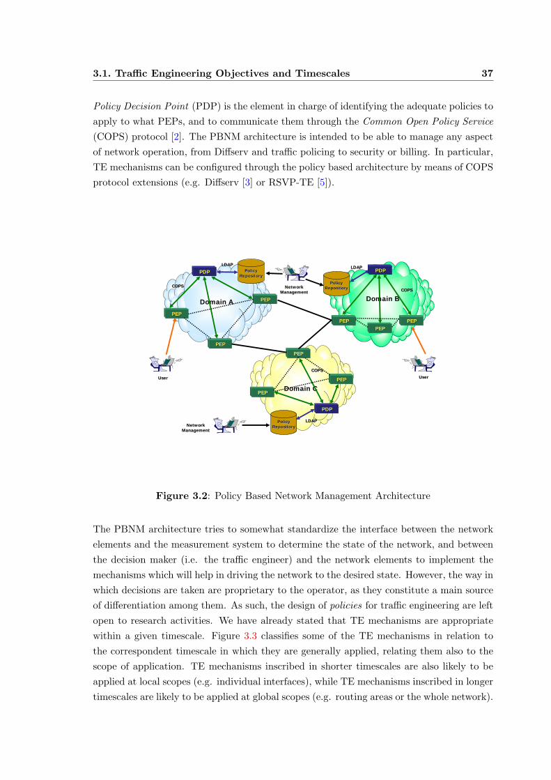
The traffic engineer, as a decision maker, will take into account the nature of the observedstate and decide to apply a particular action or set of actions. The correspondence betweena given condition and the action taken is defined as a policy. In recent years, the InternetEngineering Task Force (IETF) has made efforts towards defining an architecture capableof dealing with the complexity of the management in an evolved traffic engineering environ-ment: the Policy Based Network Management (PBNM). The Resource Allocation Protocol(RAP) working group has defined the framework, including the architectural elements [1].In Figure 3.2, the architectural elements are shown. The Policy Enforcement Points (PEPs)(i.e. routers, switches, access points) are the elements where the different TE mechanismsare applied, since they see the packets and flows traverse through them and are in a positionto change the treatment given to the traffic. The actions to be taken are stored in policyrepositories [4] in the format of policies (i.e. conditions and the corresponding actions). The
3.1. Traffic Engineering Objectives and Timescales 37
Policy Decision Point (PDP) is the element in charge of identifying the adequate policies toapply to what PEPs, and to communicate them through the Common Open Policy Service(COPS) protocol [2]. The PBNM architecture is intended to be able to manage any aspectof network operation, from Diffserv and traffic policing to security or billing. In particular,TE mechanisms can be configured through the policy based architecture by means of COPSprotocol extensions (e.g. Diffserv [3] or RSVP-TE [5]).
Domain A Domain B
Domain C
PEPPEP
PEPPEP
PEPPEP
PEPPEP
PolicyPolicyRepositoryRepository
PolicyPolicyRepositoryRepository
PolicyPolicyRepositoryRepository
LDAPLDAPLDAPLDAP
LDAPLDAPNetwork Network
ManagementManagement
Network Network ManagementManagement
PEPPEP
PEPPEP
PEPPEP
PEPPEPUserUser UserUser
PEPPEP
PDPPDP
PDPPDP
PDPPDP
COPSCOPSCOPSCOPS
COPSCOPS
Figure 3.2: Policy Based Network Management Architecture
The PBNM architecture tries to somewhat standardize the interface between the networkelements and the measurement system to determine the state of the network, and betweenthe decision maker (i.e. the traffic engineer) and the network elements to implement themechanisms which will help in driving the network to the desired state. However, the way inwhich decisions are taken are proprietary to the operator, as they constitute a main sourceof differentiation among them. As such, the design of policies for traffic engineering are leftopen to research activities. We have already stated that TE mechanisms are appropriatewithin a given timescale. Figure 3.3 classifies some of the TE mechanisms in relation tothe correspondent timescale in which they are generally applied, relating them also to thescope of application. TE mechanisms inscribed in shorter timescales are also likely to beapplied at local scopes (e.g. individual interfaces), while TE mechanisms inscribed in longertimescales are likely to be applied at global scopes (e.g. routing areas or the whole network).

38 3. Evolved Traffic Engineering
SHORT LONG
LOCAL
GLOBAL
Service Differentiation Dimensioning Planning
Congestion Control
Router Schedulingand Marking
Layout Optimizationand Reconfiguration
Load Balancing
Admission Control
Capacity Planning
Element Placing
Timescale
Scop
e
Figure 3.3: TE Mechanisms and Their Relationship to Timescales
To deal with interdependencies among the TE mechanisms, a control loop can be definedcorresponding to each of the identified timescales. Nesting the control loops, actions takenin an outer loop generate a network state that is presented to inner loops as the observedstate, so interdependencies are solved in the model. The longer timescale can then beidentified with the planning and dimensioning control loop: the network will be plannedand dimensioned taking into account the traffic forecast and the observed network state,positioning the network in an optimal state with respect to some cost function. This costfunction would take into account OAM related and deployment costs to the operator. Figure3.4 shows the different control loops and some of the actions identified with each one of them.
Once the network positioned in an optimal operational state, significative load variationswill require a new network dimensioning (and eventually a new capacity allocation scheme),resulting in a network reconfiguration. Depending on the transport technology being used,the reconfiguration in the network can involve changing the routing policies or setting up acompletely new layout (e.g. in the case of MPLS). What dimensioning and reconfigurationpolicies are to be used give rise to a bunch of research directions in the field of networkoptimization and operational research. For small load variations, redimensioning and re-configuring the network may be impractical (i.e. the cost of reconfiguration can be higherthan the cost of operating a suboptimal network). Those variations can be dealt with in an

3.1. Traffic Engineering Objectives and Timescales 39
Dimensioning
Load Variations
Measure
-
Policing/Admission
Control
Measure
-
+
+
Traffic Forecast
Traffic Demand Estimates
Load Variations
Observable Traffic
Parameters
Short Term Control Loop
Long Term Control Loop
+Load Sharing/DynamicRouting
+
Measure
+
+
-
Medium Term Control Loop
Figure 3.4: Closed Loop Traffic Engineering System
inner control loop corresponding to a medium-term timescale. Techniques such as optimalload sharing [76, 64] in the case of MPLS as transport technology, or changing the metricsof the IGP routing protocols [45] in a pure IP environment, can help to balance the load dy-namically and allow for a better efficiency of the network resources. In a shorter timescale,and for traffic variations on a user-by-user flow level, techniques such as flow control at TCPlevel [77], admission control or traffic shaping among others can be used. Here again, poli-cies on how to decide the techniques to use at medium and short term timescales give riseto a wide field of research. In this thesis, we are interested in the problems associated withthe dimensioning and reconfiguration of the network on a long-term timescale, in particularconsidering MPLS layouts. We consider that many contributions are possible in this field,since small or no attention has been paid to the dimensioning and reconfiguration optimiza-tion of layouts for transport techniques other than optical networks, taking into accountthe OAM costs as viewed by the operator and the particularities of transport technologiesassociated to the IP family like MPLS.
3.1.3. The Role of MPLS in The Traffic Engineering
The way in which traffic is routed through the network is one of the most important setof tools the operator has to meet the TE objectives. Looking in detail to the network el-ements in charge of delivering the packets at any point in the network, two steps can be

40 3. Evolved Traffic Engineering
identified: packet routing (also called the control part and packet forwarding. The IETFhas recently created a Working Group (the Forwarding and Control Element Separationforces WG to address issues regarding both functionalities). In pure IP environments, IGProuting protocols are generally used within an autonomous system to decide the routingof packets through the network. These IGPs (e.g. OSPF, IS-IS) take routing decisions ona per-packet basis, using the destination IP address as the sole information, resulting ina limited capability for the implementation of evolved TE techniques to control the trafficdistribution within the network, such as non-ECMP (Equal Cost Multipath) load sharingand general optimal routing virtual topologies among others. Also, since routing decisionsare taken hop-by-hop, the packet forwarding part doesn’t offer either much room to imple-ment evolved TE functionalities in order to offer end-to-end service differentiation and QoSguarantees. Indeed, the fact that routing decisions are taken on a hop-by-hop basis makesdifficult a coordinated packet treatment on all the interfaces used by a particular path fora given service class.
Significant work is currently undergoing to overcome the difficulties in implementing evolvedTE capabilities in an IP transport technology. In pure IP environments, the limitations ofthe IGPs to better control the traffic distribution are being addressed by dynamically chang-ing, for instance, the protocol metrics associated to each link (those used by the protocol tocalculate the routes) according to some measure of performance generally associated withcongestion [75, 45]. Protocol extensions are being considered also in order to establish routeson demand, based on service classes traffic requirements [78]. Another aspect difficult toimplement in a pure IP transport with IGPs is the load sharing functionality (i.e. to sharethe load from source to destination among multiple paths), allowing for a more efficient useof available capacity. IGP load sharing is limited to ECMP: the set of paths on which theload is shared have to be equal cost paths in terms of the protocol metrics and the loadis shared equally among them, otherwise routing loops could take place. Regarding theforwarding part of the routing function, the Differentiated Services (Diffserv [79]) and theIntegrated Services (Intserv [80]) architectures are models proposed by the IETF to providerelative service class differentiation in the former or absolute QoS guarantees in the later.However, the connectionless nature of IP routing makes difficult to implement end-to-endservice differentiation using IGPs, since no global vision of the network is available to therouting protocol at the moment of deciding the route, and packets belonging to the sameservice class are not guaranteed to receive the same (or equivalent) treatment along thewhole path, as the path can change during the life of the flow.
Multiprotocol Label Switching (MPLS) enables the possibility to implement evolved trafficengineering techniques in IP networks. These techniques allow to solve the above mentionedproblems associated to the use of IGPs in pure IP environments. MPLS architecture is de-

3.1. Traffic Engineering Objectives and Timescales 41
scribed in [8]. MPLS establishes virtual tunnels or label switched paths (LSPs), associatinga label to each LSP. A label is associated to a Forward Equivalent Class (FEC) (e.g. originand destination IP address + class of service), which ensures that all packets labelled with aparticular FEC will be delivered along the same path. In this way, routes can be decided bythe traffic engineering system using more complete network state information, and estab-lished at the origin (source routed paths). Also, as the whole path is known and all packetsbelonging to a FEC are guaranteed to be forwarded over the same path, the treatment givento all packets of that FEC can be guaranteed also to receive the same treatment, easing theimplementation of QoS guarantees. The requirements for implementing TE functionalitieswith MPLS are described in [9]. The routers implementing MPLS are called Label SwitchedRouters (LSRs); the switching of labels instead of looking up to the IP level results in animportant efficiency gain in the routers.
One important characteristic in traffic engineering is the concept of traffic trunk. A trafficaggregate is defined by the whole traffic going from a particular source to a particulardestination, and belonging to a given class of service. The problem of mapping thosetraffic aggregates on the physical network topology is a main problem in the TE. In anMPLS environment, each traffic aggregate can be directly mapped to a particular LSPs(or multiple LSPs in the case of load sharing). Those paths can be calculated to optimizea given cost function depending on performance and/or economic objectives. The virtualtopology or layout obtained (corresponding to the general optimal routing) can be whollyimplemented deploying the adequate labels, which is equivalent to establishing the virtualpaths on the network. A particular treatment can be associated to each path, adding QoSguarantees to the traffic traversing the network. In summary, MPLS allows for performanceand efficiency optimization on an IP network in many aspects:
Congestion States Produced by a Sub-Optimal Routing : The existent LSPs can be re-routed or new LSPs added in order to redistribute the traffic so as to drive the networktowards an optimal state (dimensioning and reconfiguration).
Congestion States Produced by Transitory Traffic Variations : The existent LSPs can bereconfigured to deal with non systematic traffic variations (load sharing).
MPLS support Differentiated Services (MPLS-Diffserv) [11] enables the possibility of en-gineering the different classes of service defined in the Diffserv architecture by assigningto each per-domain scheduling class (PSC) [81] a particular FEC (or set of FECs), whichensures that the appropriate treatment will be given to packets belonging to that PSC.Figure 3.5 shows the service class definition in Diffserv architecture:
PHB Group (PG): a set of one or more Per-Hop Behavior (PHB) with a common con-straint (queue servicing or management policy).

42 3. Evolved Traffic Engineering
AF1
PHBGroup
3
2
Forwarding Probability
Delay Variation
Assured Forwarding PHBAF11
AF12
AF13
Constraint = Delay Variation
3
2
1
AF2
3
2
1
AF3
3
2
1
AF4
1PHB
Figure 3.5: Diffserv PHB y PHB Scheduling Class
PHB Scheduling Class (PSC): a PHB Group with the common constraint of orderingpreservation for packets belonging to the same microflow.
Figure 3.6 shows the different types of LPS supporting Diffserv PSCs. EXP-Inferred-PSCLSP (E-LSP) uses the experimental (EXP) field defined in the MPLS header to signalthe PSCs being transported in a particular LSP (defined by the MPLS label). An E-LSPcan transport many PSCs, resulting in an efficient use of label space, but a less efficientseparation of service classes within a single LSP. A possible use of E-LSPs is, for instance,the support of service differentiation within a single Virtual Private Network (VPN): TheFEC determines the paths used by the particular VPN to transport the customer traffic,and supporting service differentiation within the VPN. In this case, the TE mechanismsnecessary to ensure the service differentiation are applied at the edge of the network, andare based mainly on traffic policing and admission control.
The Label-Only-Inferred-PSC LSPs (L-LSP) on the other hand, uses the EXP field andthe label in the MPLS header to signal the service class being transported. This meansthat each LSP transports a particular PSC (e.g. AF1 service class with the 3 droppingprecedences AF11, AF12 and AF13), offering a better separation of service classes withinthe network. Each service class could have, for instance, a dedicated LSP, which offers thepossibility of applying TE mechanisms along the path in order to offer individual guaran-tees. This advantage comes at the price of intensive label space usage.

3.2. Traffic Engineering and Measurements 43
MPLS Label IP HeaderDSCP PayloadEXP
Copy
Link LSP
3
2
1
3
2
1
EF PHB = PHB PSC
BE PHB
AF2x PSC
AF1x PSC
MPLS Label IP Header PayloadEXP
Link LSP
3
2
1AF1x PSC
Signals dropping precedence
E-LSP: MPLS Label determines FEC and EXP field determines PHB.
L-LSP: MPLS Label and EXP field determine the pair <FEC , PSC>.
Figure 3.6: MPLS-Diffserv LSP Types
MPLS appears then, as a natural solution to the difficulties found in pure IP environmentswhen implementing evolved TE functionalities. The introduction of MPLS as a transporttechnology is a key complement to IP to achieve the main objective of service integrationin a unique infrastructure, while making an efficient use of network resources. As we men-tioned before, MPLS allows the implementation of the general optimal routing layout byestablishing source routed paths copying the optimally calculated layout. As a consequence,the number of paths (LSPs) required to establish a particular layout could be specially im-portant for large networks, introducing the associated problems of layout complexity andreconfiguration. In [40], the implementation of the general optimal routing layout with amix of IGP for the compatible part of the layout and MPLS to complete the non-compatiblepart of the layout is studied. However, the design of reduced complexity layouts and thecomplexity of layout reconfiguration are open issues scarcely addressed in the literature,and are the main field of contribution in this thesis.
3.2. Traffic Engineering and Measurements
At the beginning of this chapter, we have described the TE system as a closed loop controlsystem, in which the TE mechanisms are the actions taken to drive the network to the

44 3. Evolved Traffic Engineering
desired operational state, and the observation and measurement subsystem is responsiblefor determining the current state of the network in order to make possible for the trafficengineer to take an appropriate decision. The observation and measurement sub-systemis a key element in the traffic engineering conceived as a control of the network dynamics.The observation and measurement sub-system is responsible for determining the state ofthe network based on measures integrated in the correspondent timescale. Also, basedon measures and an appropriate statistical model, it contributes to determine the trafficforecast that can be used in the capacity planning and dimensioning phases of the networkdesign. In what follows, some preliminary notions on how network states can be classifiedand observed are introduced.
3.2.1. Network States
Regarding the dynamic control concept of the TE, the network can be thought as a statemachine, where the states are optimal (i.e. desired states) or sub-optimal, and the differ-ent TE mechanisms are used to transition the network from sub-optimal states to optimalstates. Figure 3.7 presents a simplistic representation of network states that can be iden-tified according to observation and measurement within the network, and the related TEmechanisms that can be used to drive the network among states.
OptimalState
Sub-OptimalState
Congestion orOversize
Measure
Short to Medium Term TE Mechanisms
MeasureMeasure
Long Term TE Mechanisms
Measure• What?• Where?• How Often ?
How wedeterminethe optimal state?
When is thesystem in sub-optimal state?
When is thesystem congestedor overdimensioned?
Short to Medium Term TE Mechanisms
Admission Control Load Variation
Load VariationLoad Variation
Figure 3.7: TE System and Network States

3.2. Traffic Engineering and Measurements 45
Optimal State : The network is in a state defined by the operator as the optimal state withrespect to the cost functions representing its business model. In the optimal state,all the underwritten service contracts (SLAs) are honored, while efficiently using thenetwork resources according to the operator’s objectives.
Sub-Optimal State : The network is in a state defined by the operator as sub-optimal withrespect to its business objectives. In a sub-optimal state, the service contracts are stillhonored, but the network resources are no longer being used efficiently. Sub-optimalstates are generated by transitory variations in the load conditions.
Congestion or Sub-utilization State : The network is in a congestion state when servicecontracts are not honored in a systematic way, even when network resources are ef-ficiently used (although this is not likely). A congestion state is produces by a sys-tematic and significant variation in traffic load conditions (traffic increase). If servicecontracts are honored, but the network resources are being systematically used in aninefficient way, we identify the network state as a sub-utilization state. TE techniqueslike dimensioning and reconfiguration allow the operator to return to the optimal statein either case.
Each network state is univocally defined by a set of observable and/or measurable param-eters. The observation and measurement sub-system is the one responsible to infer thenetwork state from these observations and measurements. The observation implies twodifferent levels:
• Detailed: per customer and service class. It individually observes (through measure-ment) the state of the individual service contracts.
• Global: on a traffic aggregate basis within the network. It helps the operator todetermine if the network resources are correctly provisioned so as to ensure the QoSto the set of service contracts.
The combination of detailed and global observation is used by the sub-system to determinethe network state, and again, this is based on the policies configured by the operator, repre-senting mainly its business model. As such, the particular parameters and conditions thatdetermine the network state are proprietary to each operator, and constitute a source formarket differentiation.
Observation and measurement in the network can be passive or active. Passive measurementis based on the collection of information in the network without injecting measurementtraffic, while active measurement is based on special packets injected for measurementpurposes. Four main approaches have been considered [82] for gathering information fromthe network passively:

46 3. Evolved Traffic Engineering
1. The necessary traffic statistics may be available directly from Single Management Pro-tocol (SNMP) Management Information Bases (MIBs), depending on the forwardingtechnology being used (e.g. MPLS MIBs can be consulted to obtain the measuredtraffic volume on the LSPs).
2. The demands can be computed by combining packet level or flow level measurementsat the edge of the network with the information available in routing tables.
3. The demands can be inferred based on observation of the aggregate loads inside thenetwork in conjunction with routing data (this approach is known as network tomog-raphy).
4. New techniques for packet sampling offer the possibility of direct observation of thedemands as it flows through the network.
Important work is undergoing at the IETF regarding the active metrology in IP environ-ments. The IP Performance Metrics (IPPM) working group defined the framework archi-tecture [83], in which a set of metrics to measure different aspects of network performancesuch as connectivity, one way delay and one way packet loss among others are defined.Important research directions are being addressed regarding active measurement, such asdetermining the sampling frequency, statistic techniques to interpret the measures amongothers.
3.3. Contributions to the Long-term Control Loop: Dimensioning and
Reconfiguration
The long term control loop function is to establish an operational point for the network.This operational point is realized by the set of paths and the corresponding traffic beingrouted over that set of paths or layout. The main objective is to efficiently route the trafficdemands between every pair of nodes in the network. To obtain an optimal layout accordingto the operational and business objectives is one of the main problems the operator has toface. The problem of designing this optimal layout is referenced as dimensioning. Oncethis operational point established, and according to the measured traffic dynamics and theoperator’s service and business model, this operational point will have to be recalculated.The repositioning of the operational point will require a reconfiguration of the set of pathsand and the flow distributions over those new paths. The resulting reconfiguration, de-pending on the size of the network and the transport technology being used, could imply alarge amount of resources being involved in the change, resulting in a high cost of operation(maybe higher than operating the network on a sub-optimal point). A new objective associ-ated with the dimensioning arises: the optimization of the reconfiguration. In our work, weaddress both, the dimensioning and reconfiguration problems taking int account the OAM

3.3. Contributions to the Long-term Control Loop: Dimensioning andReconfiguration 47
costs as seen by the operator. Increasing attention is being paid to these problems, initiallytreated in relation to the design of optical transport networks, as the service integration atthe IP transport layer requires the introduction of technologies like MPLS.
3.3.1. Defining an Optimal Point of Operation: Network Dimensioning
As it was described in previous sections, in a pure IP environment the traditional routingprotocols calculate the route to use at each hop by calculating the shortest path based onmetrics associated to each link. To offer QoS guarantees to the different classes of service,a QoS-aware routing is the best fit to find a path meeting the constraints imposed by thedemands. The associated metrics are generally made dependent on the flow traversing thelink, so that the load conditions in the network are taken into account when calculating thebest route for every pair of nodes (and indirectly determining a working layout). However,as the metrics are dynamically updated to reflect the load conditions in the network, routeoscillations will be produced. Load sharing techniques could help in reducing the probabil-ity of the route oscillations, but in a pure IP environment, the use of load sharing is limitedto equal costs paths to avoid routing cycles.
MPLS can help introduce the required TE functionalities, while avoiding the cited problemsof route oscillation and route cycles. The fact that all packets labelled with the same FECare guaranteed to be delivered over the same route allows us to define a virtual topologyconstituted by the LSPs mapped onto the physical topology. There are two ways in whichthe optimal virtual layout can be calculated: on-line and off-line.
On-Line Layout Calculation
The idea behind on-line methods is to find a path meeting the constraints upon demandarrivals. The LSPs can be calculated to provide the required resources and to meet theservice constraints, while optimizing a particular objective function of the network perfor-mance. The resulting LSP can then be established using protocol extensions like RSVP-TE[10] or protocols intended for that purpose like CR-LDP [12].
The problem of finding an optimal path meeting a set of constraints is referenced asconstrained-based routing. Constrained-based routing constitutes an important area of re-search. The Minimum Interference routing (MIRA) algorithm [15] tries to find a pathavoiding the critically loaded paths while verifying the constraints. [25] improves uponMIRA by choosing a set of k minimum-interference paths meeting the constraints. Gener-ally used costs are related to the objective of minimizing congestion.

48 3. Evolved Traffic Engineering
Selecting the paths on-line, the long term traffic distribution in the network depends onthe order and size of demand arrivals. As a consequence, the resulting layout will not beglobally optimal with respect to a global performance objective. In that case the point ofoperation cannot be fixed, as the paths are established as needed, and calculated using localinformation on the state of the network.
Off-Line Layout Calculation
In the context of the presented TE closed loop system, we are interested in fixing an op-erational point. As such, we need to resort to an off-line calculation of the virtual layout.The off-line calculation has the advantage of allowing the use of global information, so fora given traffic demand, a globally optimal layout can be calculated with respect to a costfunction representing the OAM costs. Cost functions generally used consider transportcosts or traditional performance measures like total delay. In the present work, realisticcost functions are proposed representing the costs as seen by the operator: operation andmaintenance costs. The OAM costs in large networks are related to the complexity (i.e.number of hops and paths) needed to route a given demand. A suitable objective will bethen to minimize the complexity of the virtual layout being calculated. Each path has anassociated cost if the path is being used, representing the particular cost structure of theoperator. Given that QoS guarantees must be ensured, such as the end-to-end path delayand throughput, the calculation includes these guarantees as constraints.
The problem of minimizing the total number of paths in a layout has been already addressesin the field of optic network design and planning. The results obtained for optic networksare useful as a reference, but they cannot be directly applied to the design of MPLS layoutsbecause of the different granularities required for the IP transport layer. At the same time,the large bandwidths available in a lightpath allow for the end-to-end path delay constraintsto be expressed simply as a limit in the number of hops used in a given path, while ina MPLS context these constraints are modelled in a more realistic way given the smallerbandwidths required for each path.
A first contribution in the present work constitutes the formulation of the layout designproblem minimizing the complexity required, while meeting realistic QoS constraints im-posed by the demands.
3.3.2. Varying Traffic Conditions: Network Reconfiguration
When the traffic dynamics is considered, the point of operation is not the optimal anymore,as the traffic matrix for which the current operational layout has been calculated doesn’trepresent the current demands. A given operational point can absorb more or less important

3.3. Contributions to the Long-term Control Loop: Dimensioning andReconfiguration 49
traffic variations thanks to the TE mechanisms used inside shorter terms control loops, butfor significative changes in demand conditions, calculating a new operational point becomesunavoidable.
The new layout has to also take into account the objectives introduced in section 3.3.1.However, when the number of established paths in the current layout is large, the transitionbetween two optimal layouts in the sense of the presented objective can be very costly.Indeed, if all paths of the new layout have to be established in parallel in order to minimizeservice disruption times, the operator will have to make enough resources available for thisto happen. On the other hand, if all the paths in the new layout are set up once the paths inthe old layout have been released in order to minimize the need for spare network resources,then the service disruption time may be increased to levels incompatible with the servicecontracts. We identify the objective of minimizing the transition complexity, together withthe complexity of the new calculated layout to be an important contribution in the field ofMPLS layout design considering the traffic dynamics.


4. Contribution to the Dimensioning of MPLS Networks: Design
of Reduced Complexity Layouts
4.1. Motivations and Previous Work
Assuming that the network topology has already been deployed to optimize the cost func-tions considered in the planning phase, which includes the capacity planning and nodeplacement problems [42, 43, 44], the operator faces the problem of how to design, for agiven traffic demand, the virtual topology (i.e. the set of LSPs) mapped onto the physicaltopology. Indeed, evolved traffic engineering on source routed paths allows to split the loadof the total demand for a given node pair among the various LSPs connecting that nodepair. In this way, the optimal routing with respect to some measure of operations andmaintenance costs can be effectively implemented, by optimizing the way the total demandfor all node pairs in the network is routed through this virtual topology.
Both, off-line and on-line approaches have been proposed throughout the literature to de-sign the layout. The idea behind on-line approaches is to find a suitable path upon demandarrivals. LSPs can be calculated to meet demand requirements and service constraints, suchas available capacity and experienced delay, as well as to optimize some function of networkeconomics. Calculated paths will be established using CR-LDP [12] or RSVP-TE [10]. Inthe on-line path calculation approaches, the resulting global traffic distribution over timedepends on the arrival order and size of demands. Actual resource allocation over timecould become far from optimal with respect to some performance criteria (e.g. maximumlink load or total delay) or economic criteria (e.g. quantity of paths or links) used to designthe layout. Off-line LSP layout calculation allows for the setting up of a point of operation,globally optimal with respect to some performance criteria related to the network cost ofoperation. Off-line calculation takes into account global information about the state of thenetwork and traffic forecast, while on-line calculations are only allowed to take into accountlocal and incomplete information. In fact, on-line and off-line calculations are complemen-tary. The network can be optimally engineered and set up around a point of operationon a long term basis, and on-line decisions can be taken to accommodate traffic variationsaround that point on a shorter timescale.
Usually proposed cost functions for layout optimization consider the transport cost seen byeach user imposing a demand [22], minimizing the most loaded link in the network [23], or
51

524. Contribution to the Dimensioning of MPLS Networks: Design of Reduced
Complexity Layouts
minimizing the average cross network packet delay, subject to a delay constraint for eachorigin-destination pair [24].
In this chapter, we take into account the operation and maintenance cost of the network.In order to do so, we focus on the problem of obtaining a layout which is optimal in thenumber of required LSPs. Indeed, cost of operation in large networks in directly related tothe layout complexity. We use weights associated to each path in order to reflect a particularoperator’s cost structure. The problem of minimizing the total number of paths has beenanalyzed in the context of DWDM networks [25]. The related results cannot be applied inour context since the delay constraints cannot be expressed here just as maximum numberof hops and thus linear programming approaches are not applicable to solve our problem.We formulate the problem, which we call Minimum Path Set and Flow Allocation Problem(MPSFAP), as a Mixed Integer Non Linear Problem (MINLP). Two different cost functionsare proposed. The first one aims at minimizing a function of the total number of paths,under an end-to-end delay constraint. The second one aims at minimizing an increasingfunction of the total number of paths and of the total delay under an end-to-end delayconstraint. The second approach leads to a more homogeneously distributed load. We firstconsider a unique service class, and give QoS guarantees for it, by imposing a maximumdelay constraint on each path. The model is then extended to consider multiple serviceclasses.
4.2. Network Model Notation
For our modeling purposes, the underlying physical network provides transmission linesbetween connecting nodes. These transmission lines have an associated physical capacity.According to the traffic engineering techniques reviewed in Chapter 3, we identify the nodeswith MPLS Label Switching Routers (LSR), originating and terminating Label SwitchedPaths (LSP) over which the traffic will be transported between source and destinationnodes. The LSPs can be established using either manual or automated procedures via amanagement system through signalling protocols (e.g. CR-LDP or RSVP-TE). The LSPsare established over the transmission lines connecting the nodes, and allocated a part of theavailable capacity.
Formally, the physical network is represented by a directed graph G = (V, E), where V isthe set of vertices indexed 1, 2, . . . , N ; E is the set of directed edges indexed 1, 2, . . . ,M ,corresponding to the links in the network. Link i, corresponding to a transmission line, hascapacity Ci. Let C be the single column matrix representing the M -dimensional capacityvector.

4.2. Network Model Notation 53
Paths
The virtual topology mapped onto the physical topology allows for evolved traffic engineer-ing to be implemented on the network, making a more efficient traffic distribution possible.This efficiency stems from the fact that the traffic can be splitted among different pathsinstead along a unique path as is the case with interior gateway protocols (IGP) in a pureIP environment. Let’s assume that every pair of nodes in the physical topology is connectedthrough one or more paths, corresponding to the different LSPs in the layout. We use theterms path and LSP as synonymous.
Let the node pairs (m,n), with m 6= n, be indexed 1, 2, . . . , Q where Q = N(N − 1) isthe total quantity of node pairs. For each source-destination pair q = (m,n), we identifya commodity with the demand requested for q as dq. The commodity dq may be routedvia the Kq different acyclic paths (or routes) binding node m to node n over the graph.These paths are indexed a1
q , a2q , . . . , a
Kqq , and are known in advance. Any path akq can be
represented as a vector with entries akq,i = 1 if path akq uses link i, and 0 otherwise, fori = 1, 2, . . . ,M . As stated, we only consider acyclic paths, i.e. no path traverses twice thesame link or the same node. We can represent the K =
∑Qq=1Kq single paths between all
pair of nodes as the M ×K arc-path incidence matrix A:
A =
a11,1 ... aK1
1,1 a12,1 ... aK2
2,1 ... a1Q,1 ... a
KQ
Q,1
a11,2 ... aK1
1,2 a12,2 ... aK2
2,2 ... a1Q,2 ... a
KQ
Q,2...
......
......
...a11,M ... aK1
1,M a12,M ... aK2
2,M ... a1Q,M ... a
KQ
Q,M
The matrix A can be represented synthetically as the block matrix:
A =(A1 A2 . . . AQ
)(4.1)
where the block Aq is the arc-path matrix corresponding to the Kq paths for the node pair q.
Let W be the single column matrix representing the K-dimensional vector containing theweight wkq associated with path akq . In section 4.3 we present a way weights can be used tofine tune the path cost structure for a given operator.
Demands
In order to characterize the demands to every pair of nodes, we need to understand thenature of the IP traffic. We can analyze it at different timescales: packet and flows.

544. Contribution to the Dimensioning of MPLS Networks: Design of Reduced
Complexity Layouts
Packet Level Characteristics
It is well known that the stochastic processes describing the arrival of IP packets exhibit ahigh variability at all timescales [27]. Consequently, the use of a token bucket to describeits behavior is not well adapted. The description of IP traffic between any pair of nodesshould be made therefore in terms of flows or aggregates.
Flow Level Characteristics
A flow can be defined as a succession of packets near in time to one another, generated bythe same application instance between a particular source and destination pair. We canidentify two great categories of flow types [20]: elastic and stream flows. Stream flows arerepresentative of real-time applications (e.g. audio or video); they have intrinsic tempo-ral properties that the network must preserve. The elastic flows are representative of filetransfer-like applications. For elastic flows the transfer throughput depends on the avail-able bandwidth: the transfer duration is a function of the file size and traffic characteristicsof the transport network during the transfer. Elastic traffic is the most important of theInternet in terms of its proportion to stream traffic (approximately 80% of the flows). Todescribe the flow arrival process, the usual practice is to characterize it as a Poisson process.For the stream flow types, we can assimilate it to the arrival of voice calls, and the Poissondescription would be appropriate. For the elastic flows, a detailed study of the behavior ofa typical user during a session (e.g a web session) should be considered. However, empiricalresults show that we can appropriately assimilate the arrival process of elastic flows to aPoisson process in a given link at the core of the network [28].
Demand Characterization
Measures on Internet backbone links have shown that the traffic on those links is more orless predictable [29]. The traffic intensity presents cycles, resulting on long high utilizationperiods, followed by long low utilization periods during the day on weekdays. The sameperiodicity can be found during the weekend, but with different intensities and times of theday. This periodicity suggests that the traffic intensity could be modelled using a stationarystochastic process. More precise studies regarding the modelling of traffic processes at flowlevel can be found in [85, 86, 87]. The average measured traffic could be then interpreted asa demand with a throughput equal to the product of the flow arriving rate and the averagethroughput of the individual flows (both stream and elastic).
The use of flows allows us to better characterize the demands, and as such, to also char-acterize the QoS offered by the network. Based on these models, we can calculate therequired dimensioning to provide the required QoS guarantees. The flow level correspondsto the timescale at which we apply the traffic engineering mechanisms to control the offeredQoS (i.e. short timescale corresponds to packet level and longer timescales to flow level).In conclusion, we propose a flow level description of demands through the single columnmatrix:

4.2. Network Model Notation 55
D =
d1
d2
...dQ
(4.2)
with entry dq being the traffic value requested for the node pair q, for 1 ≤ q ≤ Q
Path Flows
The optimal dimensioning of the network with respect to an objective function given bythe operator would make use of multiple paths connecting every pair of nodes. Each pathin the set of paths between a particular source and destination is allocated a proportionof the demand for that node pair. The proportion of flow allocated to each path is also aresult of the layout optimization. Figure 4.1 shows the path flows and their relationshipto the demands and the link capacities. We can easily see that the total amount of flowallocated to the set of paths connecting a given pair of nodes must equal the demand forthat pair of nodes; this equality gives rise to the demand constrain in the mathematicalproblem formulation. In the same way, we can see that a given link is traversed by pathsconnecting different pair of nodes, so the sum of flow allocated to each of such paths mustbe less or equal the capacity of that link; this inequality gives rise to the capacity constraintin the mathematical problem formulation.
b2(2,3)
b1(2,3)
1
2
9
3
6
7
Aubervilliers
St. Lambert
Montsouris
Rennes
6
5
2
1
3
16
20
18
13
14
15
417
19
8
7
d(7,1)
d(7,2)
d(7,3)
d(7,6)
d(2,1)
d(2,3)
d(2,6)
d(2,7)
d(3,1)
d(3,2)d(3,6)
d(3,7)
d(1,2)
d(1,3)
d(1,6)
d(1,7)
d(6,1)
d(6,2)
d(6,3)
d(6,7)
demands
b1(7,1)
b2(7,1)
b3(7,1)
∑ ==
3
1 )1,7()1,7( kkbdDemand
Constraint
kq
Q
q
K
k
kq abx
q
19,1 1
19 ∑∑= =
= CapacityConstraint
VTHD Network fragment (www.vthd.org)
Figure 4.1: Path Flows: Relationship to Demands and Link Capacities

564. Contribution to the Dimensioning of MPLS Networks: Design of Reduced
Complexity Layouts
Formally, let the flow assigned to path akq be denoted by bkq . The single column matrixrepresenting the path flows is:
B =
b11...bK11...
b1Q...
bKQ
Q
(4.3)
Let us define R = (rq,i) the Q×K commodity-path incidence matrix, where entry rq,i = 1if i lies in the interval [K1 +K2 + . . .+Kq−1 +1,K1 +K2 + . . .+Kq−1 +Kq] and 0 otherwise,for 1 ≤ q ≤ Q and 1 ≤ i ≤ K. We assume no flow loss, hence the sum of the flows for theKq paths connecting the node pair q must satisfy the demand dq, for all 1 ≤ q ≤ Q:
R ·B = D (4.4)
Let xi be the value of the total flow traversing link i, for 1 ≤ i ≤M , and let X be the singlecolumn matrix representing the M dimensional vector of total flows for all links:
X = A ·B (4.5)
4.3. Building the Cost Functions
The cost of operation for large networks is related to the layout complexity [16]. We definecomplexity as the number of paths necessary to transport a given demand matrix D. In-deed, the operations and maintenance costs are related to the quantity of paths to establishwhen setting up the layout and then maintained once the layout is in place. Traditionally,objectives for layout optimization consider the minimization of some measure of networkperformance. Functions of total cross network delay or link load [22, 23, 24] are generallyproposed as objectives for layout optimization. Layouts obtained with these objectives willdistribute the flows on the paths so as to equalize the loads on the links, resulting in a lowdelay variation from link to link. Models proposing those objective functions assume a costproportional to the use of the capacity, which is not realistic in terms of operations andmanagement costs from an operator’s standpoint. As we discussed in previous chapters,the cost of capacity deployment is already considered in the capacity planning phase. Weare focusing on the dimensioning of the network (i.e. the obtention of a layout and flowallocations) given the physical topology.

4.3. Building the Cost Functions 57
To minimize OAM costs we need to take into account some function of layout complexity,provided that the QoS guarantees given to the customers are always met. We introduce away to provide these QoS guarantees through constraints in the optimization problem insection 4.4. The objective will be then to minimize a function of the general form:
Minimize
Q∑q=1
Kq∑k=1
wkqhkq
(4.6)
where hqk is a binary variable indicating if the corresponding path akq is in use or not. Wedefine H as a single column matrix, whose entries hkq are defined as follows:
hkq =
1 if bkq > 0
0 otherwise(4.7)
The objective function of the form given in (4.6) will minimize the weighted sum of the bi-nary variables. The weight associated to each path represents then the cost that the set-upof such path has for the operator. The way in which such weights are defined can be usedby the operator to fine tune the cost structure of the network OAM.
If the path weights are independent of the path flow, the layouts optimizing the objectivefunction (4.6) will tend to concentrate the flow on fewer paths. One of the consequencesof this result is that experienced end-to-end delay along the different paths connecting anygiven pair of nodes will exhibit a great dispersion from the average for that group of paths.If a packet-based routing strategy is to be used, this dispersion will produce a high rateof resequencing at the end nodes, since IP packets using paths with different end-to-enddelay will not arrive in order to the destination. If a flow-based routing strategy is to beused, the need for resequencing is minimized, since packets belonging to the same flow willtraverse the same path. In order to minimize the dispersion in the end-to-end path delayon the layout, we propose an alternative objective function, which makes appear a secondterm taking into account the total cross network delay:
Minimize
α Q∑q=1
KQ∑k=1
wkqhkq + β
Q∑q=1
Kq∑k=1
hkq
M∑i=1
λakq,iCi − xi
(4.8)
Assuming that it is appropriate in our model to approximate the link delay1 by an M/M/1queueing system [30], the second term in 4.8 will produce layouts which tend to equalizethe load distribution through the network, while keeping the complexity low. The factors α
1Neglecting packetization and transmission delays

584. Contribution to the Dimensioning of MPLS Networks: Design of Reduced
Complexity Layouts
and β help us in controlling the relative importance of each term in the objective function,and λ is the average packet size. Indeed, as we expressed in section 4.2, we are assumingthat a Poisson process is a good model for the flow arrival process. At the same time, asthe dimensioning refers to the network core, the flows are seen at an aggregate level. Thehypotheses to apply the Kleinrock independence approximation for each link delay thenhold2.
Path Weights
The weights wkq associated with each path can be used by the operator to fine tune thecost structure of the path layout. For instance, setting the weights on a hop-count basis,the operator can introduce the fact that setting up shorter paths is less expensive for itsmanagement and maintenance cost structure than setting up paths with longer hop-counts:
wkq =M∑i=1
akq,i k = 1, . . . ,Kq; q = 1, . . . , Q (4.9)
In particular, hop-count based weights minimize a function of the number of used links.Setting all the weights to 1 minimizes the total number of paths. Operators having differentcost structures might use these weights to represent their own operational costs. In whatfollows, we use (4.9) to calculate the weights associated to each path. As results show,minimizing the total number of links, indirectly minimizes the total number of used paths,and we assure at the same time that shortest paths (in terms of hops) are taken first.
4.4. Setting QoS Guarantees
If no performance measures are included in the objective function, we need a way to ensurethat QoS guarantees are met. These guarantees will then be introduced in the problemformulation as constraints. Those constraints ensure that no path will exceed a flow al-location on component links that violates the required QoS objectives. We are interestedin providing two types of QoS guarantees: throughput and end-to-end delay. The demandconstraints ensure that enough bandwidth is allocated to the set of paths connecting anygiven pair of nodes, so as to guarantee the throughput for that node pair. Identifying acommodity with all the demand for the node pair q, the bandwidth guarantee is given forthe total demand dq:
dq =Kq∑k=1
bkq (4.10)
2Assuming packet sizes exponentially distributed, a densely connected network and moderate to heavy load

4.4. Setting QoS Guarantees 59
Paths in this context will then be identified as transporting an aggregate of traffic, and guar-antees are given for that aggregate. A discussion about different alternatives on guaranteesfor multiple classes of service (both absolute and relative) is given in section 4.7.
Guarantees for delay are given through the end-to-end path delay constraints. Any givenpath in the set of paths connecting a given node pair q, which has an allocated path flowbkq > 0, cannot exceed a given end-to-end maximum allowed delay θq:
hkq
M∑i=1
λakq,iCi − xi
≤ θq (4.11)
for all the paths in the set k = 1, . . . ,Kq connecting the node pair q. Again, this guaranteeis given for any packet of the aggregate dq traversing any path connecting the node pair q.A discussion about separate guarantees given for different classes of service on the aggregatedq is given in section 4.7.
It is important to note here that the end-to-end path delay constraint should be appliedto used paths only (i.e. paths with a positive flow allocation). Indeed, the path delay fora given commodity not only depends on the value of its own traffic, but also on the trafficissued by all the other paths sharing the same links, as can be seen in an example depictedin Figure 4.2, and Table 4.1.
1 2
3
b �
�
b �
�b �
�
b �
�
1
2 3
d �
d �
d �
d �
d �
d �
Figure 4.2: Example on the importance of avoiding path-delay constraints on unused paths
In the referred example, packets sent along the path a21 would see a total delay of 18.18
msec., which is greater than the maximum allowed delay θ1 = 10 msec. This violatedconstraint will prevent paths a1
2 and a13 from being able to carry the corresponding flows to
meet the demands. If no path delay constraint is imposed on unused paths, both a12 and
a13 will be able to carry the flows b12 and b13 to meet the demands without violating any
constraint.

604. Contribution to the Dimensioning of MPLS Networks: Design of Reduced
Complexity Layouts
commodities
q (s, d) dq(bps) θq(msec)
1 (1, 2) 890 10
2 (1, 3) 890 10
3 (3, 2) 890 10
links
link Ci(bps) xi(bps)
1 1000 890
2 1000 890
3 1000 890
paths
akq links bk
q (bps) τkq (msec)
a11 1 890 9.09
a21 2, 3 0 18.18
a12 2 890 9.09
a13 3 890 9.09
τkq is the calculated end-to-end path delay
for path akq
Table 4.1: Example on the importance of avoiding path-delay constraints on unused paths
4.5. Formulation: Minimum Path Set and Flow Allocation Problem (MPSFAP)
Given the network physical topology and the traffic matrix, the problem is to find a setof paths and the flow allocation over those paths in order to optimize a cost objective,complying to some QoS constraints. In this section we formulate the problem of designingthe optimal layout w.r.t. the complexity of the layout (as defined in section 4.3, whilemeeting some QoS guarantees (i.e. end-to-end path delay and available bandwidth pernode pair). The Network Design Multicommodity Flow Allocation Problem in its matrixform is stated as follows:
MPSFAP 1Minimum Path Set and Flow Allocation Problem
Given:
A,C,D,Θ,∆,W
minimize :
tW ·H (4.12)
subject to:
X = A ·B ≤ C (4.13)R ·B = D (4.14)
hkq
M∑i=1
λakq,iCi − xi
≤ θq k = 1, . . . ,Kq; q = 1, . . . , Q (4.15)
bkq ≤ hkqδq k = 1, . . . ,Kq; q = 1, . . . , Q (4.16)
hkq ∈ {0, 1} k = 1, . . . ,Kq; q = 1, . . . , Q (4.17)
bkq ≥ 0 k = 1, . . . ,Kq; q = 1, . . . , Q (4.18)

4.5. Formulation: Minimum Path Set and Flow Allocation Problem(MPSFAP) 61
where Θ is the column matrix containing the maximum tolerable delay θq for each com-modity dq and ∆ is the column matrix containing the maximum flow δq acceptable on onepath for the commodity dq.
Similarly, we can define a problem MPSFAP 2 using the objective function (4.8) to takecare of the flow distribution in the layout:
MPSFAP 2Minimum Path Set and Flow Allocation Problem Considering Flow Distribution
Given:
A,C,D,Θ,∆,W
minimize :
α tW ·H + β
Q∑q=1
Kq∑k=1
hkq
M∑i=1
λakq,iCi − xi
(4.19)
subject to:
X = A ·B ≤ C (4.20)R ·B = D (4.21)
hkq
M∑i=1
λakq,iCi − xi
≤ θq k = 1, . . . ,Kq; q = 1, . . . , Q (4.22)
bkq ≤ hkqδq k = 1, . . . ,Kq; q = 1, . . . , Q (4.23)
hkq ∈ {0, 1} k = 1, . . . ,Kq; q = 1, . . . , Q (4.24)
bkq ≥ 0 k = 1, . . . ,Kq; q = 1, . . . , Q (4.25)
Constraints (4.13)/(4.20) and (4.15)/(4.22), both impose limitations in the usable capacityon each link. However, the constraints (4.15)/(4.22) are more restrictive in the sense thatsolutions meeting these constraints, will also meet the constraints (4.13)/(4.20) for all links.We keep all constraints in our formulation for clarity, but they will be automatically simpli-fied in the presolve phase of the solvers. The additional constraints (4.16)/(4.23) are usefulto prevent paths for a given commodity to take all the available capacity of a particular link(e.g. if we want to make possible to share a critical link among paths connecting differentnode pairs and provide bandwidth guarantees for each path), or to somewhat control apriori the load sharing granularity when designing the layout (i.e. we know that each pathfor commodity dq will not transport more than δq units of bandwidth).
In section 4.6 we compare results obtained for both MPSFAP 1 and MPSFAP 2 for small
624. Contribution to the Dimensioning of MPLS Networks: Design of Reduced
Complexity Layouts
networks.
4.6. Preliminary Results on MPSFAP and Model Validation
The MPSAFP problems are network design multicommodity flow problems, since the binaryvariables hkq make decisions on whether a path is to be included in the solution or not, andthe continuous flow variables bkq indicate the quantity of flow to be allocated to each of theselected paths. The MPSFAP 1 problem can be seen as solving two related problems atthe same time: one 0-1 network design problem as only the binary variables are presentin the objective function, and a constraint satisfaction problem on the path flow variables.The set of paths is given through the arc-path incidence matrix A. The commodity-pathincidence matrix R indicates which of those paths connect what node pairs. The resultingMPSFAP are Mixed Integer Non-Linear Programming (MINLP) problems, since they havea combination of integer (hkq ) and continuous (bkq ) variables, and a set of linear and non-linear constraints.
Constrained global optimization is NP-complete, because it takes exponential time to ver-ify whether a feasible solution is optimal or not for a general constrained NLP [32, 33].Besides, the MPSFAP problems lie in the category of general MINLP problems, which areNP-complete [34, 35]. Even if we formulate the problem using piecewise linear constraintsfor the path delay instead of the original non-linear constraints, the resulting MILP problemis known to be also NP-complete. Replacing the non-linear constraints however is not prac-tical in the context of the design of MPLS layouts, since we need to make no assumptionson the underlying transport technologies, whenever they provide links with an associatedavailable capacity. The underlying transport infrastructure will then provide links with dif-ferent capacities, leading to a different piecewise linear function for each possible capacityvalue. This adds to the size of an already large and complex problem, relativizing the gainsobtained by formulating a MILP problem instead of a MINLP problem. We resort then toheuristics to efficiently solve the MPSFAP problems in Chapter 5.
The MPSFAP problems are particularly difficult to solve due to their size and complex-ity. We use a path formulation instead of a flow formulation in order to reduce the sizeof the problem [14], but we pay the price of having an enormous set of variables. TheMPSFAP problems have two variables for each path: one integer variable representing thedecision variable of the network design problem, and one continuous variable representingthe amount of flow to allocate to that particular path in the constraint satisfaction prob-lem (in particular for the MPSFAP 1 problem, which we consider the most interesting interms of practicality as we can safely assume flow-by-flow routing in the network core).The quantity of variables is 2K, where K is the total number of paths connecting every

4.6. Preliminary Results on MPSFAP and Model Validation 63
pair of nodes (i.e. the number of rows in the arc-incidence matrix). The number of allpossible paths will typically be enormous, growing exponentially with the network size [14].MPSFAP problems have Q demand constraints, M capacity constraints, and K path de-lay constraints, in addition to the nonnegativity conditions imposed on the path flow values.
Due to the limitations imposed by the size of the problems to solve, we first obtain prelim-inary results from a solver for small networks. The objective is to validate the model andobtain a first insight on the results obtained in view of the heuristics to develop in the nextchapter.
4.6.1. Traffic Matrixes
Traffic demands are randomly generated according to the following method, which is in-spired in the method described in [25]. A certain proportion p of the node-pairs are assigneda demand flow following a random variable uniformly distributed within the interval [0, Cq
a ],where Cq is the total capacity available for connecting the node pair q if no traffic is flowingthrough the network, and a is an arbitrary integer to help us in scaling the traffic intensitywhen all node pairs are considered. Indeed, increasing a would produce traffic matrixeswith larger probability of being feasible solutions for a given network topology. To modelsome degree of asymmetry in the network, we allow a proportion (1− p) of the node pairsto have traffic demands uniformly distributed in the interval [0, CqY
a ]. We define Y as theratio maxq{Cq}
minq{Cq} , which are the capacity of the best connected node pairs and the capacity ofthe worst connected node pairs in the network respectively.
A set of 25 traffic matrixes are randomly generated for each of the test topologies describedin section 4.6.2.
4.6.2. Network Topologies
In order to study the problem and validate the model we resort to two small sized networktopologies, so that the size of the problem is tractable by known solvers in the domain.The network topologies proposed are a 4-node network with 8 and 10 (directed) links re-spectively. We denote these test topologies by NET1 and NET2. Figure 4.3 shows thecorresponding network topologies.
Link capacities for both networks are set to 2.5 Gbps for all links. NET1 has a total of24 possible paths, generating a problem of 48 variables and 68 constraints (besides thepath flow positivity conditions and the simplifications in the presolve phase of the solver).Similarly, NET2 has a total of 38 possible paths, generating a problem of 76 variables and

644. Contribution to the Dimensioning of MPLS Networks: Design of Reduced
Complexity Layouts
98 constraints. These problem sizes allow us to obtain preliminary results useful to evaluatethe interest of the proposed cost functions.
��� ��� �
2.5 Gbps
2.5 Gbps
2.5 Gbps
2.5 Gbps
�� ��� �
��� ��� � �� ��� �
(a) NET1
��� ��� �
2.5 Gbps
2.5 Gbps
2.5 Gbps
2.5 Gbps
�� ��� �
��� ��� � �� ��� �
2.5 Gbps
2.5 Gbps
(b) NET2
Figure 4.3: NET1 and NET2 Networks.
4.6.3. Reference Problem
One of the most used cost functions through the optimization literature is a measure ofnetwork performance such as total delay in the network. We are interested in evaluatingthe complexity of the layouts created with our proposed cost functions to the complexity oflayouts obtained with a cost function minimizing total delay in the network. We proposethen a reference problem which minimizes total cross network delay, and we will denotethis problem by Minimum Total Delay Flow Allocation Problem (MTDFAP). The proposedobjective for MTDFAP is to minimize:
Q∑q=1
Kq∑k=1
hkq
M∑i=1
λakq,iCi − xi
(4.26)
for all pairs q = 1, . . . , Q, subject to the same constraints as defined for the MPSFAPproblems (4.13)(4.15)(4.14) for MPSFAP1, and (4.20)(4.22)(4.21) for MPSFAP2. MTDFAPis also formulated as a MINLP problem. Unfortunately, the MTDFAP problem can not beused to compare our results for larger networks using the proposed heuristics in Chapter 6because of the size of the problem instances generated.
4.6.4. Interface to Solvers: Modeling Language
As a first approach to solving the MPSFAP problems, numeric solvers can help to get aninsight in the problem structure and complexity. A numeric solver can help also in validat-

4.6. Preliminary Results on MPSFAP and Model Validation 65
ing the problem formulations through the use of a formal mathematical modeling languageextensively used in the field of operations research. We have searched first for a suitablesolver, since they are generally adapted to a very narrow type of problem and particularstructures of the associated matrixes. We resorted to a well-known source of solver imple-mentations, which makes available a set of solvers, categorized by problem type and inputinterface: the NEOS server on the Internet [18, 37, 38].
The MINLP solver [19] available through NEOS server provides the solution of mixed in-teger nonlinearly constrained optimization problems in AMPL format. MINLP is suitablefor large nonlinearly constrained problems with a modest number of degrees of freedom.MINLP implements a branch-and-bound algorithm searching a tree whose nodes correspondto continuous nonlinearly constrained optimization problems. The continuous problems aresolved using filterSQP [39], a Sequential Quadratic Programming solver which is suitablefor solving large nonlinearly constrained problems.
AMPL is a mathematical modeling language, which provides a standardized way of repre-senting or modeling a problem. If we wanted to present a solver with a particular instanceof a problem, we would have to change the equation system (right hand side terms, quan-tity of equations, coefficients in equations, etc.) according to each instance. If we used amodeling language instead, we would present the solver with a model of the problem, whichdescribes its structure, and then the solver would be capable of instantiate every problemaccording to the data associated. There are two common modeling languages widely usedin the operational research world: A Modeling Language for Mathematical Programming(AMPL) [36], and General Algebraic Modeling System (GAMS) [84]. Solvers are increas-ingly being developed to accept one or both of the input formats. The solver must thenimplement an AMPL or GAMS compilator to create the problem instances with the asso-ciated data presented at its input. Once the instance created (correctness of the model anddata is checked during compilation), the solver executes a presolve phase to detect whetherthe problem can be simplified (constraints and variables eliminated or transformed). Thesimplified problem is then passed to the solver.
4.6.5. Results and Analysis
Solutions for NET1 and NET2 for 25 traffic matrixes generated according to the model insection 4.6.1 are obtained from the exact (deterministic) MINLP solver available throughthe NEOS server. Solution for MPSFAP1 and MPSFAP2 problems are compared to thesolutions obtained for the MTDFAP problem using the same parameters and topologies.Both MPSFAP1 and MPSFAP2 problems have associated path weights wkq set to the num-ber of hops used by the path. Parameters are set to δq = 2.5 Gbps. (i.e. the path flows can

664. Contribution to the Dimensioning of MPLS Networks: Design of Reduced
Complexity Layouts
use up to the maximum available capacity in any link), end-to-end path delay limits θq areset to 30 µsec. The factors α and β are set to 1 for the MPSFAP2 problem. The set of 25traffic matrixes are generated with parameters a = 3 and a = 4 for the NET1 network; anda = 5 and a = 6 for NET2 network. In all cases, we use p = 0.2, meaning that 20% of nodepairs are allowed demands up to Y = 1 (there are exactly 2 possible paths connecting everypair of nodes in NET1) times larger for NET1 and Y = 1.33 (there are some node pairsconnected through 2 paths and some connected through 3 paths in NET2) times larger forNET2.
NET1 - Hops and Paths
Matrix
a = 4 / p = 0.2 a = 3 / p = 0.2
MTDFAP MPSFAP1 MPSFAP2 MTDFAP MPSFAP1 MPSFAP2
Paths Hops Paths Hops Paths Hops Paths Hops Paths Hops Paths Hops
1 12 16 12 16 12 16 14 20 12 16 12 16
2 12 16 12 16 12 16 12 16 12 16 12 16
3 12 16 12 16 12 16 13 18 12 16 12 16
4 13 18 12 16 12 16 I I I I I I
5 12 16 12 16 12 16 12 16 12 16 12 16
6 13 18 12 16 12 16 I I I I I I
7 12 16 12 16 12 16 13 18 13 18 13 18
8 13 18 12 16 12 16 13 18 13 18 13 18
9 13 18 12 16 12 16 14 20 14 20 14 20
10 12 16 12 16 12 16 13 18 13 18 13 18
11 12 16 12 16 12 16 13 18 12 16 12 16
12 12 16 12 16 12 16 14 20 13 18 13 18
13 12 16 12 16 12 16 13 18 12 16 12 16
14 12 16 12 16 12 16 12 16 12 16 12 16
15 12 16 12 16 12 16 12 16 12 16 12 16
16 12 16 12 16 12 16 I I I I I I
17 12 16 12 16 12 16 12 16 12 16 12 16
18 12 16 12 16 12 16 13 18 12 16 12 16
19 13 18 12 16 12 16 13 18 12 18 13 18
20 12 16 12 16 12 16 13 18 12 16 12 16
21 12 16 12 16 12 16 I I I I I I
22 12 16 12 16 12 16 13 18 12 16 12 16
23 12 18 12 16 12 16 I I I I I I
24 12 16 12 16 12 16 12 16 12 16 12 16
25 12 16 12 16 12 16 13 18 12 16 12 16
Averages 12.20 16.40 12.00 16.00 12.00 16.00 12.85 17.70 12.30 16.70 12.35 16.70
Table 4.2: Quantity of Hops and Paths for MTDFAP, MPSFAP1 and MPSFAP2 Problemswith NET1 Network
Table 4.2 and Table 4.3 show the quantity of hops and paths in the solution for the MTD-FAP, MPSFAP1 and MPSFAP2 problems for NET1 and NET2 respectively. In both tables,the value I indicates an integer infeasible problem as declared by the solver. A set of 25demand matrixes is generated for each of two load situations, corresponding to mild andheavy load. For NET1 a mild load condition is found with a = 4 (all problems feasible), andheavy load with a = 3 (20% of the matrixes resulted in infeasible problems). For NET2, amild load condition is found with a = 6 (all problems feasible), and a heavy load is foundwith a = 5 (24% of the problems infeasible). After problem simplification (presolve) all theproblem instances for NET1 generated a total of 48 linear variables, 24 linear constraintsand 44 non-linear constraints, while the problems instances for NET2 generated a total of76 linear variables, 38 linear constraints and 60 non-linear constraints. The quantity ofvariables and constraints generated by these simple network topologies give us a taste of

4.6. Preliminary Results on MPSFAP and Model Validation 67
the complexity of the problem larger networks would generate.
The time consumed at the solver server for all problem formulation and all instances ofNET1 is under 10 seconds, while the time consumed for NET2 under the same conditionsis higher than 100 seconds. We see a time increase of about 10 times when adding a pair oflinks in the topology (increasing from 24 to 38 possible paths).
Results for NET1 in Table 4.2 show that the number of hops in the layouts resultingfrom MPSFAP1 and MPSFAP2 are always lower than those in the layouts obtained fromMTDFAP. Under a mild load (a = 4), MPSFAP1 and MPSFAP2 use in average 2.5% lesstotal hops than MTDFAP. When the load increases (a = 3), MPSFAP1 and MPSFAP2 usea 5, 99% less total hops than MTDFAP. Looking at the quantity of paths, results show thatfor mild load MPSFAP1 and MPSFAP2 produce layouts with 1.67% less paths than thoseproduced by MTDFAP, while for heavy load MPSFAP1 and MPSFAP2 produce layoutswith around 4.5% less paths than those produced by MTDFAP.
a=4 / p=0.2
0,00
1,00
2,00
3,00
4,00
5,00
6,00
7,00
1 2 3 4 5 6 7 8 9 10 11 12 13 14 15 16 17 18 19 20 21 22 23 24 25Matrixes
mic
rose
c.
Avg Path Delay - MTDFAPAvg Path Delay - MPSFAP1Avg Path Delay - MPSFAP2
(a) a = 4
a=3 / p=0.2
0,00
2,00
4,00
6,00
8,00
10,00
12,00
14,00
1 2 3 4 5 6 7 8 9 10 11 12 13 14 15 16 17 18 19 20 21 22 23 24 25Matrixes
mic
rose
c.
Avg Path Delay - MTDFAPAvg Path Delay - MPSFAP1Avg Path Delay - MPSFAP2
(b) a = 3
Figure 4.4: Average End-to-end Path Delay for NET1
At first sight, both MPSFAP1 and MPSFAP2 produce layouts with the same quantity ofhops and paths. Figure 4.4 shows the average end-to-end path delay for mild and heavyload situations. Figure 4.5 shows the maximum end-to-end path delay obtained for everymatrix on the set for mild and heavy load situations.
Average end-to-end delay on paths in layouts produced by MPSFAP1 are noticeably higherthan those on paths produced by MTDFAP, and the difference increases with the load.Average end-to-end delay on paths in layouts produced by MPSFAP2 are closer to those onpaths in layouts produced by MTDFAP. Correspondingly, we see that a higher number ofpaths reach the maximum allowed end-to-end delay for MPSFAP1 when the load increases,while paths in layouts produced by MPSFAP2 and MTDFAP rarely reach the maximum

684. Contribution to the Dimensioning of MPLS Networks: Design of Reduced
Complexity Layouts
a=4 / p=0.2
0,00
5,00
10,00
15,00
20,00
25,00
30,00
35,00
1 2 3 4 5 6 7 8 9 10 11 12 13 14 15 16 17 18 19 20 21 22 23 24 25Matrixes
mic
rose
c.
Max Path Delay - MTDFAPMax Path Delay - MPSFAP1Max Path Delay - MPSFAP2
(a) a = 4
a=3 / p=0.2
0,00
5,00
10,00
15,00
20,00
25,00
30,00
35,00
1 2 3 4 5 6 7 8 9 10 11 12 13 14 15 16 17 18 19 20 21 22 23 24 25Matrixes
mic
rose
c.
Max Path Delay - MTDFAPMax Path Delay - MPSFAP1Max Path Delay - MPSFAP2
(b) a = 3
Figure 4.5: Maximum End-to-end Path Delay for NET1
allowed end-to-end delay (delay constraint).
NET2 - Hops and Paths
Matrix
a = 6 / p = 0.2 a = 5 / p = 0.2
MTDFAP MPSFAP1 MPSFAP2 MTDFAP MPSFAP1 MPSFAP2
Paths Hops Paths Hops Paths Hops Paths Hops Paths Hops Paths Hops
1 13 16 12 14 12 14 13 16 13 16 13 16
2 14 19 12 15 12 15 I I I I I I
3 12 15 12 14 12 14 12 15 12 14 12 14
4 13 16 12 14 12 14 13 16 13 16 13 16
5 13 16 12 14 12 14 14 18 13 16 13 16
6 12 16 12 15 12 15 I I I I I I
7 12 14 12 14 12 14 12 14 12 14 12 14
8 12 14 12 14 12 14 13 16 12 14 12 14
9 12 16 12 15 12 15 I I I I I I
10 14 18 12 15 12 15 I I I I I I
11 12 16 12 15 12 15 13 17 12 16 12 16
12 12 14 12 14 12 14 13 16 12 14 12 14
13 12 14 12 14 12 14 13 17 12 14 12 14
14 13 17 13 16 13 16 I I I I I I
15 12 16 12 15 12 15 13 18 12 15 12 15
16 12 14 12 14 12 14 12 14 12 14 12 14
17 12 16 12 14 12 14 12 16 12 15 12 15
18 13 16 12 14 12 14 13 16 13 16 13 16
19 12 15 12 15 12 15 13 18 12 15 12 15
20 12 14 12 14 12 14 12 14 12 14 12 14
21 13 18 12 15 12 15 14 20 14 19 14 19
22 12 16 12 14 12 14 12 16 12 15 12 15
23 13 16 12 15 12 15 13 16 13 16 13 16
24 12 16 12 14 12 14 13 17 12 15 12 15
25 14 18 14 18 14 18 I I I I I I
Averages 12.52 15.84 12.12 14.60 12.12 14.60 12.79 16.32 12.37 15.16 12.37 15.16
Table 4.3: Quantity of Hops and Paths for MTDFAP, MPSFAP1 and MPSFAP2 Problemswith NET2 Network
Results in Table 4.3 show similar trends as results for NET1 in all three problems. In thiscase, the savings in quantity of hops is of about 8% for MPSFAP1 and MPSFAP2 in allload situations. Similarly, the savings in quantity of paths is of about 3.5% under the sameconditions. Figures 4.6 and 4.7 show the average and maximum end-to-end delay for NET2respectively on paths in layouts obtained with MTDFAP, MPSFAP1 and MPSFAP2 undermild and heavy load conditions.

4.6. Preliminary Results on MPSFAP and Model Validation 69
a=6 / p=0.2
0,00
2,00
4,00
6,00
8,00
10,00
12,00
1 2 3 4 5 6 7 8 9 10 11 12 13 14 15 16 17 18 19 20 21 22 23 24 25Matrixes
mic
rose
c.
Avg Path Delay - MTDFAPAvg Path Delay - MPSFAP1Avg Path Delay - MPSFAP2
(a) a = 6
a=6 / p=0.2
0,00
2,00
4,00
6,00
8,00
10,00
12,00
14,00
1 2 3 4 5 6 7 8 9 10 11 12 13 14 15 16 17 18 19 20 21 22 23 24 25Matrixes
mic
rose
c.
Avg Path Delay - MTDFAPAvg Path Delay - MPSFAP1Avg Path Delay - MPSFAP2
(b) a = 5
Figure 4.6: Average End-to-end Path Delay for NET2
a=6 / p=0.2
0,00
5,00
10,00
15,00
20,00
25,00
30,00
35,00
1 2 3 4 5 6 7 8 9 10 11 12 13 14 15 16 17 18 19 20 21 22 23 24 25Matrixes
mic
rose
c.
Avg Path Delay - MTDFAPAvg Path Delay - MPSFAP1Avg Path Delay - MPSFAP2
(a) a = 6
a=5 / p=0.2
0,00
5,00
10,00
15,00
20,00
25,00
30,00
35,00
1 2 3 4 5 6 7 8 9 10 11 12 13 14 15 16 17 18 19 20 21 22 23 24 25Matrixes
mic
rose
c.
Avg Path Delay - MTDFAPAvg Path Delay - MPSFAP1Avg Path Delay - MPSFAP2
(b) a = 5
Figure 4.7: Maximum End-to-end Path Delay for NET2
These results suggest that when the network size increases, the savings in quantity of hopsand paths can be more significative, encouraging the development of heuristics which wouldallow us to obtain layouts minimizing complexity for larger networks in order to realize op-eration and maintenance cost savings. The reason for the increase in savings when networkdensity increases is quite obvious: a denser network presents more paths connecting everypair of nodes. As MTDFAP tries to minimize the total delay in the network, the optimalsolution would be to use as much paths as possible, charging each path to a minimum soas to make the delay on each path as low as possible, the limit given by the critical links,which will set the lower bound delays on any path traversing them. Results also show thateven when the objective function aims at minimizing the total number of hops in the layoutthrough the choice of the path weights defined in equation (4.9), the number of total pathsgets also minimized.

704. Contribution to the Dimensioning of MPLS Networks: Design of Reduced
Complexity Layouts
4.7. Extensions for Multiple Classes of Service
In section 4.4 we defined a commodity as an aggregate of traffic to be transported from nodem to node n. As such, all packets belonging to the same aggregate are transported throughthe set of paths connecting the corresponding node pair, all receiving the guarantees givenfor that set of paths. If classes of service (CoS) are considered within each aggregate, thenwe need to do something in order to individually meet the QoS guarantees for each CoS oneach path. As discussed in chapter 3, we have two approaches to solve this issue. The firstapproach will still consider a commodity as all the traffic to be transported from node mto node n. In this case, the problem stays the same as before, where we need to establishthe optimal layout for a given set of demands, and the QoS guarantees are globally metfor all classes of services on each path through the constraints introduced in the MPSFAPproblems. Individual relative guarantees could be given to each individual CoS within eachpath through service differentiation mechanisms (e.g. using Diffserv-aware LSPs). The sec-ond approach considers instead all the traffic aggregate for a single class of service to betransported between node m and node n as a commodity. Here, each path in the set ofpaths connecting a given node pair will transport a fraction of the traffic of a single CoSdemanded between that node pair, so that individual QoS guarantees can be given to eachCoS for each node pair.
The first approach is trivial from the point of view of problem formulation. The secondapproach needs a little bit of work to extend the model to multiple classes of service. Inthis section, we present the model extensions needed to formulate MPSFAP for multipleclasses of service. It is worth noting that the extended problem will generate even largerinstances than those generated for a single class in a particular network topology. Thismakes the development of heuristics even more interesting in the context of dimensioningIP next generation networks, where service differentiation and individual QoS guaranteesare a strong requirement.
Formally, let us suppose that each pair q has now a demand composed of one or moreservice classes. Each pair can now originate and terminate more than one commodity. Letus extend the demand matrix to include a column for each class l indexed 1, . . . , L. Thedemand is now represented by a matrix D:
D =
d1,1 . . . d1,L
d2,1 . . . d2,L
......
...dQ,1 . . . dQ,L
(4.27)

4.7. Extensions for Multiple Classes of Service 71
The path flow matrix B is now modified to include the flow associated to each class ofservice:
B =
b11,1 . . . b11,L...
......
bK11,1 . . . bK1
1,L...
......
b1Q,1 . . . b1Q,L...
......
bKQ
Q,1 . . . bKQ
Q,L
(4.28)
The weight matrix W, is here a K × L matrix containing the weights associated to thepaths connecting a pair q for a given commodity dq,l. Calculating the weights for MPSFAPusing (4.9) will produce equal path weights for all classes of service demanded between agiven pair. Economic factors and particular service needs can be introduced through thechoice of path weights (e.g. shortest paths in terms of number of hops would be preferredfor classes associated with real time service). Accordingly, the matrix H is extended toindicate whether a given path akq is used (entry hkq,l = 1) or unused (entry hkq,l = 0) by thecommodity dq,l. Similar extensions are made to the matrixes Θ and ∆. X must now becalculated as A · B · 1lL, where 1lL is a L-dimensional column matrix with all its entriesset to 1. MPSFAP is extended to a Minimum Path Set and Flow Allocation Problem withMultiple Classes of Service (MPSFAPQ).
A MPSFAPQ1 problem can be then defined, where W(l) and H(l) are the l column of thecorresponding matrixes W and H. Similarly, δq,l is a limit in the quantity of flow acceptableon one path for a given commodity. As before, constraints (4.33) impose a limit on any pathto the quantity of flow for a particular CoS and node pair. When dimensioning for multipleclasses of service, traffic engineering can benefit of imposing such constraints in order toachieve the planified bandwidth limits for each class on critical links. The formulation inMPSFAPQ is compatible with the Diffserv aware traffic engineering in MPLS [11].
A MPSFAPQ2 problem can be similarly defined to take care of the delay variation amongpaths transporting the same commodity. The objective function (4.8) can be then extendedto include multiple classes of service:
Minimize
α Q∑q=1
KQ∑k=1
L∑l=1
wkq,lhkq,l + β
Q∑q=1
Kq∑k=1
L∑l=1
hkq,l
M∑i=1
λakq,iCi − xi
(4.36)

724. Contribution to the Dimensioning of MPLS Networks: Design of Reduced
Complexity Layouts
MPSFAPQ 1Reduced Complexity Layout with End-to-End Delay Guarantees - QoS Extension: MultipleClasses of Service
Given:
A,C,D,Θ,W
minimize :
L∑l=1
tW(l) ·H(l) (4.29)
subject to:
A ·B · 1lL ≤ C (4.30)R ·B = D (4.31)
hkq,l
M∑i=1
λakq,iCi − xi
≤ θq,l l = 1, . . . , L; k = 1, . . . ,Kq; q = 1, . . . , Q (4.32)
0 ≤ bkq,l ≤ hkq,lδq,l l = 1, . . . , L; k = 1, . . . ,Kq; q = 1, . . . , Q (4.33)
hkq,l ∈ {0, 1} l = 1, . . . , L; k = 1, . . . ,Kq; q = 1, . . . , Q (4.34)
bkq,l ≥ 0 l = 1, . . . , L; k = 1, . . . ,Kq; q = 1, . . . , Q (4.35)
4.8. Conclusions
The problem of obtaining optimal routing schemes is a well known issue in the field of net-work flow problems with application to communication and transport networks. In thosecontexts, the usual objectives are related to the use of paths in order to globally ensurea minimum congestion when transiting the network. When dealing with telecommunica-tion networks such objectives are usually kept. Given that in a pure IP environment it ispractically impossible to find a unique metric allowing to implement a fully optimal generalrouting scheme using a routing protocol [40], we resort to source routing schemes. In par-ticular, layouts established as MPLS LSPs allow the implementation of any general optimalrouting. Paths are calculated and established by the management system. However, whilea minimum congestion layout is a common optimal routing objective, it is not representa-tive of the cost of operations and maintenance incurred by an operator when establishinga given routing scheme through a source routed layout. With this in mind, from a set oflayouts capable of transporting a given demand within certain QoS bounds given by theunderwritten service contracts, an operator would chose those which guarantee a minimumcost for their operational structure.

4.8. Conclusions 73
A first contribution in our work is the definition of a minimum complexity layout as theoptimization objective. Whenever the QoS guarantees are met, considering the operator’sobjectives, the optimal layout is the one which minimizes the quantity of elements to man-age during operation: the quantity of links and paths that the layout globally uses totransport a given demand. Important work on the subject consider the optimization ofcongestion based objective functions without considering end-to-end QoS guarantees (suchas path-delay), both in the on-line and off-line contexts [15, 22, 23, 45, 46, 47]. The maininterest being the development of algorithms and heuristics to solve the resulting complexproblem. End-to-end path delay constraints have been considered so far in the context ofmulticonstrained route selection [48], routing from one source to all destinations [49, 50],or optimizing virtual circuit layouts [24], but the cost functions still consider congestionbased objectives, and the path-delay is generally modelled as a hop-count constraint. Theissue of layout complexity for MPLS layouts has particularly been addressed in [88], whererestrictions to the number of paths allowed to traverse any given link are imposed as a wayof reducing the quantity of labels needed at every hop. The resulting problem can be formu-lated as a MIP (Mixed Integer Linear Program), as the end-to-end path delay constraintsare not included. This allows to exactly solve large instances of the problem by techniquessuch as Lagrangean Decomposition. The definition of end-to-end path delay constraintsas bundling constraints in the problem formulation constitutes the second contribution inour work, as the end-to-end path delay associated to hop-count is not realistic in the con-text of MPLS networks as it is in the context of optical network design due to its coarsebandwidth granularity and broadband nature. However, some simplifications in the pathdelay constraints are necessary to implement suitable heuristics, as we describe further inChapter 5. As discussed, the non-linearities in our problem formulation are introduced bythe end-to-end path delay constraints, which constitute one of the main contributions inour work. We could try to linearize the non-linear constraints in order to be able to applyLagrangean Decomposition. To do so, we would need to linearize a large number of delayconstraints, as a different piecewise linear function is needed for each different capacity.Although this is possible to do, we prioritize then the choice of offering a fine granularityto the layout design, and then we need to develop the heuristic methods presented in nextchapter to approximately solve the problem for large networks.


5. Contribution to the Development of Heuristics for Solving the
Minimum Path Set and Flow Allocation Problems (MPSFAP)
5.1. Exact Methods for Solving MINLP Problems
The Minimum Path Set and Flow Allocation Problems (MPSFAP) are formulated in Chap-ter 3 as Mixed-Integer Non-Linear Programming (MINLP) problems. MINLP problems areNP-complete, what makes its resolution intractable for large instances. For computation-ally tractable problem sizes, exact or deterministic algorithms can be used to find optimalsolutions. When the problem size becomes larger, we must resort to heuristic methods,which yield approximated optimal solutions. Deterministic algorithms use implicit enu-meration and tree search rules, with evaluation techniques to determine whether a givensolution is optimal or not. Deterministic algorithms commonly used for exact solution ofMINLP problems range within one of the following types:
Branch and Bound (B&B)
The B&B algorithm for MINLP problems [51, 52] is based on the same ideas as B&B forsolving MILP problems. The first step is to solve the problem generated by relaxing theintegrality condition on the variables. If the solution of that problem fulfils all integralityconditions the whole problem is solved. Otherwise, in a minimization problem the relaxedproblem provides a lower bound (of course only if the global minimum can be determined)and the search tree is built up. A feasible integer solution provides an upper bound. Amajor drawback of B&B applied to MINLP problems is that nodes deeper in the tree cannotbenefit so greatly from information available at previous nodes as is the case in MILP B&Busing the dual simplex algorithm. A variant of B&B method called Extended Cutting Plane(ECP) [57] does not solve the NLP subproblems. Instead, it relies exclusively on successivelinearizations.
Generalized Benders Decomposition (GBD)
Generalized Benders Decomposition [53] divides the variables into two sets: complicat-ing and non-complicating variables. In MINLP models the class of complicating variablesis made up by the discrete (usually binary) variables. Then the algorithm generates asequence of NLP sub-problems (produced by fixing the binary variables) and solves the
75

765. Contribution to the Development of Heuristics for Solving the Minimum
Path Set and Flow Allocation Problems (MPSFAP)
so-called MILP Master problems in the space of the complicating variables. The NLP sub-problems yield upper bounds for the original problem while the MILP Master problemsyield additional combination of binary variables for subsequent NLP sub-problems. Underconvexity assumptions the Master problems generate a sequence of lower bounds increasingmonotonically. The algorithm terminates if lower and upper bounds equal or cross eachother.
Outer Approximation (OA)
Outer Approximation [54, 55] also consists of a sequence of NLP sub-problems produced byfixing the binary variables generated by MILP Master problems. The significant difference ishow the Master problems are defined. Algorithms based on OA describe the feasible regionas the intersection of an infinite collection of sets with a simpler structure (e.g. polyhedra).In OA the Master problems are generated by outer approximations (e.g. linearizations orTaylor series expansions) of the nonlinear constraints in those points which are the optimalsolutions of the NLP subproblems (i.e. a finite collection of sets). The key idea is to solvethe MINLP with a much smaller set of points (i.e. tangential planes). In convex MINLPproblems, a superset of the feasible region is established. Thus, the OA Master problems(MILP problem in both discrete and continuous variables) produce a sequence of increasinglower bounds. The termination criterion is the same as in GBD.
The problem subclasses of MINLP, Mixed Integer Linear Programming (MILP) and Non-Linear Programming (NLP), present different degrees of difficulty. MILP are combinatorialproblems for which branch and bound techniques with linear programming (LP) relaxationis often proven to be sufficient. NLP problems can only be solved iteratively. NLP problems,however are usually easier to solve than MILP problems. MINLP combines all the difficul-ties of its subclasses, adding other difficulties of its own: while for convex NLP problemsthe local minimum is identical to the global minimum, the same property does not hold forconvex MINLP problems; even when assuming convexity in the MINLP problem could beuseful, it constitutes no guarantee of finding a global minimum.
In recent years a new trend has emerged in the formulation and solution of mixed-integeroptimization problems: the Generalized Disjunctive Programming (GDP). The basic ideabehind GDP is to use boolean and continuous variables, and to formulate the problem withan objective function and subject to three type of constraints: global inequalities inde-pendent of integer decisions, disjunctions that are conditional constraints involving an ORoperator, and pure logic constraints that involve only the boolean variables. The interest inthis method resides in that it simplifies the problem formulation. Further details on GDPare out of the scope of this thesis, as our focus is on models for network optimizations in

5.2. Meta-Heuristics: Tabu Search Methods 77
the context of dimensioning and reconfiguration, as well on heuristics allowing to obtaingood enough approximated solutions in times compatible with the dynamic control of thenetwork. However, it constitutes an interesting research direction for extending the presentwork.
We have presented here some details about the deterministic methods and some well-knownalgorithms to solve general MINLP problems. The MINLP solver used in Chapter 4 to ob-tain results for the small network topologies NET1 and NET2 implement some of the abovedescribed techniques [56]. The different methods used by the deterministic solvers lead ingeneral to the need of solving a large number of NLP subproblems when applied to theMPSFAP formulated here, since the number of integer variables increases with the numberof paths, which grows exponentially with the size and density of the network. Linearizingthe constraints would help in reducing the NLP subproblems to LP subproblems (enablingmore efficient implementations of B&B for instance), but the number of subproblems tosolve would still be prohibitively large considering our objective. Our main interest liesthen in the development of algorithms implementing heuristics capable of avoiding the needto solve such a large number of subproblems. It is worth noting that our main objectivehowever, is not to develop algorithms to improve existing methods and algorithms largelystudied and implemented in the field of operations research, but to find heuristics capableof yielding good approximations to the optimal solution, which will allow us to study theproposed problems. Two heuristic methods to intelligently explore the solution space with-out solving a large number of subproblems are presented next. The first uses Tabu Search(TS) techniques to explore the solution space, while the second modifies the well-know flowdeviation algorithm used in the classical literature [64, 31] and a particular implementation[65] to solve our MINLP formulation of MPSFAP problems. In Chapter 8, a further im-provement to the Modified Flow Deviation (MFD) algorithm produces solutions for largenetworks for the dimensioning and reconfiguration problem defined in Chapter 7.
5.2. Meta-Heuristics: Tabu Search Methods
Optimization algorithms based on meta-heuristics have recently gained interest becausethey are able to cope with problem instances of large size, overcoming the complexity issuesof most problems found in practical applications. Among others, Simulated Annealing (SA)[58], Genetic Algorithms (GA) [59] and Tabu Search (TS) [60, 61] have been proposed totackle multicommodity flow problems. The computed solution however is not guaranteedto be optimal. That is why it is necessary to check the accuracy of the solutions providedby such a heuristic based algorithm and to compare them with exact solutions on small sizeproblems. A detailed description of the TS algorithm can be found in [60].

785. Contribution to the Development of Heuristics for Solving the Minimum
Path Set and Flow Allocation Problems (MPSFAP)
The TS basic idea consists in exploring the complex space of solutions until a defined num-ber of iterations is reached or until a specific cost criterion is satisfied. The explorationstarts with an initial solution computed by another algorithm (e.g. an initial solution ran-domly generated). At each iteration, TS computes a set or neighborhood of solutions derivedfrom the current solution via perturbations applied to this solution. All the solutions of theneighborhood are evaluated (i.e. assigned a value according to a cost function) and thebest one is selected as the new current solution. In order to prevent the algorithm fromcycling along the same series of current solutions, a tabu list is maintained, which containsa number of last visited solutions that cannot be chosen as long as they belong to this list.This allows the algorithm to choose a solution worse than the current one, allowing it toescape from the local minima possibly found during the search.
Formally, let N (s) be the neighborhood of a given solution s in the space of solutions S.N (s) is obtained by applying an elementary transformation to s. The method can be viewedas an iterative technique which explores a set of problem solutions by repeatedly movingfrom one solution s to another solution s′ located in the neighborhood N (s) of s. The movesaim at efficiently reaching a solution which qualifies as good (i.e. optimal or near-optimal)with respect to some objective function f(s) to be minimized. Using classic descendantmethods to search the solution space (i.e. choosing a solution s′ for which f(s′) < f(s)) willlead to get trapped in local minima for non-convex objectives; the local minima will dependupon the way the initial point was generated. To avoid getting trapped in local minima, thesearch procedure must allow some solution for which f(s′) > f(s), so as to explore differentregions of the solution space. But accepting a solution s′ that may be worse than s mayproduce cycling. To avoid this, TS adds a memory of the visited solutions, forbidding thesearch process to visit a solution which is in a tabu list of already evaluated solutions. Theconcept of memory can be formally stated by saying that the neighborhood also depends onthe iteration, so we denote it now by N (s, j), being j the iteration in which s was visited.We can now write a pseudo code with the general TS idea:
Generate an initial solution s ∈ Ss∗ := sj := 0while the stopping condition is not met doj := j + 1Generate V∗ ⊆ N (s, j)Choose the best s′ in V∗if f(s′) < f(s∗) thens∗ := s′
end ifend while
Algorithm 5.1: Pseudo-code for the General Tabu Search Method
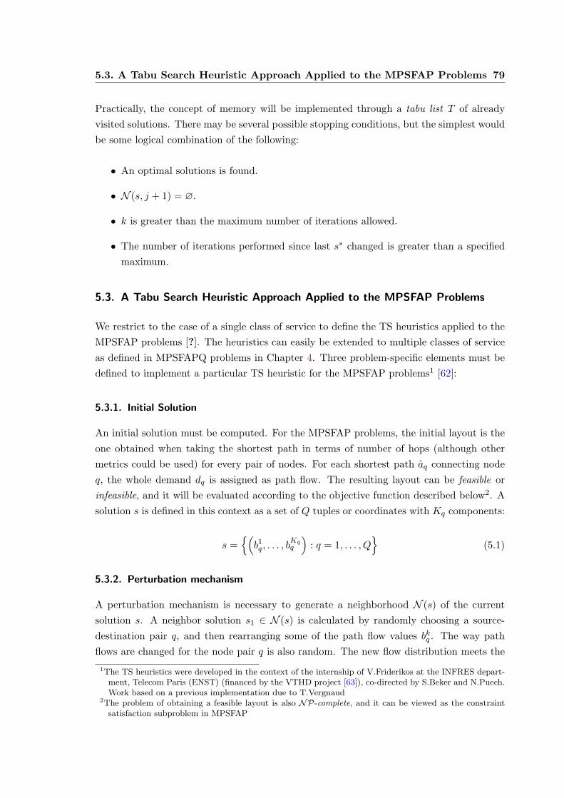
5.3. A Tabu Search Heuristic Approach Applied to the MPSFAP Problems 79
Practically, the concept of memory will be implemented through a tabu list T of alreadyvisited solutions. There may be several possible stopping conditions, but the simplest wouldbe some logical combination of the following:
• An optimal solutions is found.
• N (s, j + 1) = ∅.
• k is greater than the maximum number of iterations allowed.
• The number of iterations performed since last s∗ changed is greater than a specifiedmaximum.
5.3. A Tabu Search Heuristic Approach Applied to the MPSFAP Problems
We restrict to the case of a single class of service to define the TS heuristics applied to theMPSFAP problems [?]. The heuristics can easily be extended to multiple classes of serviceas defined in MPSFAPQ problems in Chapter 4. Three problem-specific elements must bedefined to implement a particular TS heuristic for the MPSFAP problems1 [62]:
5.3.1. Initial Solution
An initial solution must be computed. For the MPSFAP problems, the initial layout is theone obtained when taking the shortest path in terms of number of hops (although othermetrics could be used) for every pair of nodes. For each shortest path aq connecting nodeq, the whole demand dq is assigned as path flow. The resulting layout can be feasible orinfeasible, and it will be evaluated according to the objective function described below2. Asolution s is defined in this context as a set of Q tuples or coordinates with Kq components:
s ={(b1q , . . . , b
Kqq
): q = 1, . . . , Q
}(5.1)
5.3.2. Perturbation mechanism
A perturbation mechanism is necessary to generate a neighborhood N (s) of the currentsolution s. A neighbor solution s1 ∈ N (s) is calculated by randomly choosing a source-destination pair q, and then rearranging some of the path flow values bkq . The way pathflows are changed for the node pair q is also random. The new flow distribution meets the
1The TS heuristics were developed in the context of the internship of V.Friderikos at the INFRES depart-ment, Telecom Paris (ENST) (financed by the VTHD project [63]), co-directed by S.Beker and N.Puech.Work based on a previous implementation due to T.Vergnaud
2The problem of obtaining a feasible layout is also NP-complete, and it can be viewed as the constraintsatisfaction subproblem in MPSFAP

805. Contribution to the Development of Heuristics for Solving the Minimum
Path Set and Flow Allocation Problems (MPSFAP)
demand constraints but not necessarily meets the link flow and path delay constraints. Thenumber of node pairs which are to have their path flows changed when generating eachneighbor is a parameter of the algorithm. The number of neighbors to generate from thecurrent solution is also a parameter of the algorithm. The first parameter, the number ofnode pairs to have their path flows changed is a compromise between the aggressiveness ofthe solution space exploration and the computation complexity of the algorithm. Hence,the neighbor generation process leads to new candidate solutions that may be consideredas valid (i.e. solutions that meet all the constraints) or invalid (i.e. solutions that do notmeet the link flow or path delay requirements).
5.3.3. Evaluation Functions
A cost function f : S → R mapping elements in the solution space S to real numbers mustbe defined so as to allow comparison of the different solutions in the neighborhood N (s) ofthe current solution s. Since we allow infeasible layouts as initial solution, we must ensurethat the evaluation of invalid solutions in the neighborhood of the current one will drive theexploration of the solution space towards feasible or valid solutions. We use a cost functionthat evaluates distinctly valid and invalid solutions. Indeed, not all invalid solutions are thesame, and we must evaluate them differently. According to the constraint being violated inthe solution, we can distinguish two types of invalidity:
Type-1 Invalidity: A solution s is invalid because at least one of the link capacity con-straints (4.13)/(4.20) is violated.
Type-2 Invalidity: A solution s is invalid because all the capacity constraints are met,but at least one of the path delay constraints (4.15)/(4.22) is violated.
Practically, we want the evaluation to be as computationally inexpensive as possible. Byevaluating only capacity constraints first, we only perform M invalidity checks (there are Mlinks in the network), if we found the solution to be type-1 invalid, then no further evaluationmust be performed. If we found the solution not to be type 1-invalid, then further evaluationis necessary to decide wether it is type-2 invalid or valid. K type-2 invalidity checks areperformed, where K is the total number of paths in the arc-incidence matrix A (K canbe a very large number). Valid solutions are evaluated using the corresponding objectivefunctions for MPSFAP1 and MPSAP2 (depending on the problem to be solved). A givensolution s is evaluated as follows:

5.3. A Tabu Search Heuristic Approach Applied to the MPSFAP Problems 81
f(s) =
MPSFAP1(s)/MPSFAP2(s) if s is valid
g1(s) if s is Type-1 Invalid
g2(s) if s is Type-2 Invalid
(5.2)
we rewrite the objective functions MPSFAP1 and MPSFAP2 here for convenience:
MPSFAP1(s) =Q∑q=1
Kq∑k=1
wkqhkq (5.3)
MPSFAP2(s) = α
Q∑q=1
Kq∑k=1
wkqhkq + β
Q∑q=1
Kq∑k=1
hkq
M∑i=1
akq,iλ
Ci − xi
=Q∑q=1
Kq∑k=1
hkq
(αwkq + β
M∑i=1
aq,iλ
Ci − xi
) (5.4)
with all variables defined as before (Chapter 4). We are interested in ensuring that evalu-ation for type-1 invalid solutions will be always greater than evaluation for type-2 invalidsolutions. At the same time, we must ensure that evaluation for type-1 or type-2 invalidsolutions is always greater than evaluation for valid solutions using either MPSFAP1 orMPSFAP2 evaluation. We know that MPSFAP2 evaluations are always greater than eval-uations of the same solution with MPSFAP1 (α > 0 and β > 0 by definition). We can thenestablish the following relationship:
g1(s) > g2(s) > MPSFAP2(s) > MPSFAP1(s) (5.5)
In this way, valid solutions will be preferred over type-2 invalid solutions, and type-2 invalidsolutions will be preferred over type-1 invalid solutions. At the same time, a mechanismsto provide a slope within type-1 invalid solutions must be provided, so as to guide theexploration of the solution space towards type-2 invalid or valid solutions. The evaluationof type-1 invalid solutions can then be defined as:
g1(s) =M∑i=1
g′1(xi) +Q∑q=1
Kq∑k=1
wkq +Q∑q=1
Kq∑k=1
1
=M∑i=1
g′1(xi) +Q∑q=1
Kq∑k=1
(wkq + 1
) (5.6)
where g′1(xi) is defined as:

825. Contribution to the Development of Heuristics for Solving the Minimum
Path Set and Flow Allocation Problems (MPSFAP)
g′1(xi) =
xi−CiCi
if xi > Ci
0 otherwise(5.7)
for every link i = 1, . . . ,M in the network. The first term in (5.6) provides a degree ofinvalidity for the type-1 invalid solutions. It measures the degree of violation in the linkcapacities constraint in order to provide a slope towards type-2 invalid or valid solutions.Similarly, The evaluation of type-2 invalid solutions is defined as:
g2(s) =Q∑q=1
Kq∑k=1
hkqg′2(τ
kq ) +
Q∑q=1
Kq∑k=1
wkq
=Q∑q=1
Kq∑k=1
(hkqg
′2(τ
kq ) + wkq
) (5.8)
where g′2(τkq ) is defined as:
g′2(τkq ) =
τkq −θq
θqif τkq > θq
0 otherwise(5.9)
for k = 1, . . . ,Kq and q = 1, . . . , Q (all paths connecting a node pair and all node pairs).τkq is the calculated delay for path akq in the current solution. As with g1(s), the first termin (5.8) provides a degree of invalidity for the type-2 invalid solutions. It measures thedegree of violation in the path delay constraints in order to provide a slope towards validsolutions. The second and third terms in (5.6) ensure that g1(s) is greater than an evalua-tion of any type-2 invalid solution, since the second term supposes that all paths are used,and third term supposes that all paths are overloaded in terms of g2(s) evaluation. Simi-larly, the second term in (5.8) ensures that an evaluation of any type-2 invalid solution willbe greater than an evaluation of any valid solution, since it supposes that all paths are used.
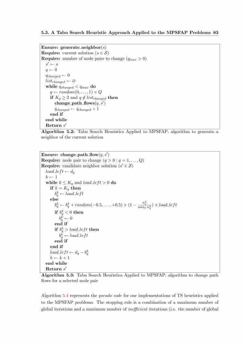
5.3. A Tabu Search Heuristic Approach Applied to the MPSFAP Problems 83
Ensure: generate neighbor(s)Require: current solution (s ∈ S)Require: number of node pairs to change (qmax > 0)s′ ← sq ← 0qchanged ← 0listchanged ← ∅while qchanged < qmax doq ← random(0, . . . , 1)×Qif Kq ≥ 2 and q /∈ listchanged then
change path flows(q, s′)qchanged ← qchanged + 1
end ifend whileReturn s′
Algorithm 5.2: Tabu Search Heuristics Applied to MPSFAP: algorithm to generate aneighbor of the current solution
Ensure: change path flow(q, s′)Require: node pair to change (q > 0 : q = 1, . . . , Q)Require: candidate neighbor solution (s′ ∈ S)load left← dqk ← 1while k ≤ Kq and load left > 0 do
if k = Kq thenbkq ← load left
elsebkq ← bkq + random(−0.5, . . . ,+0.5)× (1− wk
q
maxk wkq)× load left
if bkq < 0 thenbkq ← 0
end ifif bkq > load left thenbkq ← load left
end ifend ifload left← dq − bkqk ← k + 1
end whileReturn s′
Algorithm 5.3: Tabu Search Heuristics Applied to MPSFAP: algorithm to change pathflows for a selected node pair
Algorithm 5.4 represents the pseudo code for our implementations of TS heuristics appliedto the MPSFAP problems. The stopping rule is a combination of a maximum number ofglobal iterations and a maximum number of inefficient iterations (i.e. the number of global

845. Contribution to the Development of Heuristics for Solving the Minimum
Path Set and Flow Allocation Problems (MPSFAP)
iterations since the the algorithm didn’t produce an improvement in the evaluation). Theparameter neighbormax defines the total number of neighbors to generate during the currentiteration. The best neighbor of all generated neighbors is then evaluated and compared tothe evaluation of the current solution. If it doesn’t evaluate better than the current solution,it is put in the tabu list so it would not be visited again. If it evaluates better than thecurrent solution, then it is adopted as the current solution. Algorithm 5.2 generates asmany neighbors as defined by the parameter neighbormax. For each neighbor, it selects asmany node pairs to have their path flows changed as defined by the parameter qmax. Anode pair can only have its path flows rearranged if it has more than one path in the setof paths connecting it. Indeed, it will not be possible rearrange the path flow for a uniquepaths, as it has to carry the whole demand dq. The path flows for each of the selected nodepairs are changed as described in the algorithm 5.3. Path flows are increased or decreasedwith equal probability. The quantity of flow to be increased or decreased on a given path israndomly calculated, with a relative weight according to the path weights of the paths inthe set: paths with lower weights have higher probability of receiving or losing flow.

5.3. A Tabu Search Heuristic Approach Applied to the MPSFAP Problems 85
Require: maximum number of global iterations (iterationmax > 0)Require: maximum number of global inefficient iterations (iterationmaxinef > 0)Require: number of neighbors to generate (neighbormax > 0)
Generate an initial solution (s ∈ S)s∗ ← sT ← ∅iteration← 0iterationinef ← 0while iteration < iterationmax and iterationinef < iterationmaxinef do
for neighbor = 1 to neighbormax dos′ ← generate neighbor(s)if neighbor = 1 thens← s′
end ifif f(s′) < f(s) and s′ /∈ T thens← s′
end ifend forif f(s) ≥ f(s) thenT ← siterationinef ← iterationinef + 1
elses∗ ← siterationinef ← 0
end ifiteration← iteration+ 1s← s∗
end whileAlgorithm 5.4: Pseudo-code for the Tabu Search Heuristics Applied to the MPSFAPProblems
5.3.4. Evaluation of TS Heuristics for MPSFAP
To evaluate the TS heuristics for the MPSFAP problems, we run the algorithm for the setof 25 matrixes and network topologies NET1 and NET2 used in Section 4.6 in Chapter 4 .We then compare the results obtained from TS with the results obtained from the MINLPsolver. In this context, since the MINLP solver yields exact optimal solutions, the totalcost of the solutions constitute a reference for optimality. The number of global iterationsof the TS algorithm is set to 20, while the number of inefficient iterations is set to 10. 200neighbors are generated for the current solution in each iteration of the algorithm. We findthat having the path flows of 2 node pairs changed when generating a neighbor from thecurrent solution is a good tradeoff between the speed of progression in the solution spaceand computational effort needed.

865. Contribution to the Development of Heuristics for Solving the Minimum
Path Set and Flow Allocation Problems (MPSFAP)
Table 5.3 shows the average values of the objective function for the set of demand matrixesconsidered. f(s)MINLP corresponds to the value of the objective function obtained fromthe MINLP solver in Chapter 4, and f(s)TS the average evaluation obtained from theTS heuristics (for both problems MPSFAP1 and MPSFAP2). The evaluation functionf(s) become the objective function given by (4.6), with wkq calculated as in (4.9) when theproblem is feasible. This allows us to compare the values of the objective functions obtainedfrom the two methods directly for feasible problems. To establish a comparison betweenthe results obtained from MINLP and TS, we define f(s)%TS as follows:
f(s)%TS =f(s)TS − f(s)MINLP
f(s)MINLP100 (5.10)
MPSFAP1 MPSFAP2
f(s)MINLP f(s)TS f(s)%TS f(s)MINLP f(s)TS f(s)%TS
NET1a = 3/p = 0.2 16.70 18.68 11.86 16.73566 17.84925 6.91
a = 4/p = 0.2 16.00 17.20 7.50 16.01753 16.30396 1.79
NET2a = 5/p = 0.2 15.16 16.74 8.18 15.1943 16.07869 5.82
a = 6/p = 0.2 14.60 15.88 8.77 14.62582 15.66635 7.11
Table 5.1: Quality of the Solutions from TS with respect to MINLP for MPSFAP1 andMPSFAP2
It can be seen from the values of f(s)%TS that MPSFAP problems can be approximatedby the TS heuristics with an acceptable error. Solutions obtained for MTDFAP in Chapter4, evaluated with the objective functions of MPSFAP1 and MPSFAP2 yield close valuesin average than those obtained from TS. This means that, even when the approximationsare good enough, we are obtaining layouts with TS that are not better in terms of the costfunctions considered than those obtained when optimizing a classic performance objectivesuch as total delay.
Hops
MPSFAP1 MPSFAP2 MTDFAP
MINLP TS MINLP TS MINLP
NET1a = 3/p = 0.2 16.70 18.68 16.70 17.80 17.70
a = 4/p = 0.2 16.00 17.20 16.00 16.28 16.40
NET2a = 5/p = 0.2 15.16 16.74 15.16 16.05 16.32
a = 6/p = 0.2 14.60 15.88 14.60 15.64 15.84
Table 5.2: Comparison of Average Quantity of Hops from MINLP and TS for MPSFAP1and MPSFAP2
However, it can be seen that the approximation gets better as the size of the network in-creases. Indeed, as the network size increases (or the network gets more densely connected),the diversity of paths available also increases, offering a larger number of possible combi-

5.3. A Tabu Search Heuristic Approach Applied to the MPSFAP Problems 87
nations to be tried. In conclusion, as there is more room (solution space) to explore, theexploration becomes more effective and the solutions approach the optimal. Unfortunately,solutions for larger networks obtained from TS cannot be compared to those obtained withthe reference solver MINLP, as problem size limitations arise with the last for networkslarger than those already considered. However, solutions from TS for large networks canbe compared with solutions from the heuristic algorithm presented next, which will be alsoreferenced to the solutions obtained from the MINLP solver for NET1 and NET2 topologies.
Tables 5.2 and 5.3 show the average hop-count and path-count obtained from TS andMINLP for all cases considered. Figures 5.1 and 5.2 show the compared results for eachmatrix. Points without value in the graphs represent infeasible matrixes.
NET1 (a=3/p=0.2)
10,00
12,00
14,00
16,00
18,00
20,00
22,00
24,00
26,00
28,00
30,00
1 2 3 4 5 6 7 8 9 10 11 12 13 14 15 16 17 18 19 20 21 22 23 24 25Matrix
Hop
s
0,00
1,00
2,00
3,00
4,00
5,00
6,00
7,00
8,00
9,00
10,00
11,00
12,00
13,00
14,00
15,00
16,00
17,00
18,00
Path
s
Hops - MPSFAP1 (NEOS)
Hops - MPSFAP1 (TS)
Paths - MPSFAP1 (NEOS)
Paths - MPSFAP1 (TS)
(a) MPSFAP1, a = 3
NET1 (a=3/p=0.2)
10,00
12,00
14,00
16,00
18,00
20,00
22,00
24,00
26,00
28,00
30,00
1 2 3 4 5 6 7 8 9 10 11 12 13 14 15 16 17 18 19 20 21 22 23 24 25Matrix
Hop
s
0,00
1,00
2,00
3,00
4,00
5,00
6,00
7,00
8,00
9,00
10,00
11,00
12,00
13,00
14,00
15,00
16,00
17,00
18,00
19,00
20,00
Path
s
Hops - MPSFAP2 (NEOS)
Hops - MPSFAP2 (TS)
Paths - MPSFAP2 (NEOS)
Paths - MPSFAP2 (TS)
(b) MPSFAP2, a = 3
NET1 (a=4/p=0.2)
10,00
12,00
14,00
16,00
18,00
20,00
22,00
24,00
26,00
28,00
30,00
1 2 3 4 5 6 7 8 9 10 11 12 13 14 15 16 17 18 19 20 21 22 23 24 25Matrix
Hop
s
0,00
1,00
2,00
3,00
4,00
5,00
6,00
7,00
8,00
9,00
10,00
11,00
12,00
13,00
14,00
15,00
Path
s
Hops - MPSFAP1 (NEOS)
Hops - MPSFAP1 (TS)
Paths - MPSFAP1 (NEOS)
Paths - MPSFAP1 (TS)
(c) MPSFAP1, a = 4
NET1 (a=4/p=0.2)
10,00
12,00
14,00
16,00
18,00
20,00
22,00
24,00
26,00
28,00
30,00
1 2 3 4 5 6 7 8 9 10 11 12 13 14 15 16 17 18 19 20 21 22 23 24 25Matrix
Hop
s
0,00
1,00
2,00
3,00
4,00
5,00
6,00
7,00
8,00
9,00
10,00
11,00
12,00
13,00
14,00
Path
s
Hops - MPSFAP2 (NEOS)
Hops - MPSFAP2 (TS)
Paths - MPSFAP2 (NEOS)
Paths - MPSFAP2 (TS)
(d) MPSFAP2, a = 4
Figure 5.1: Results from MINLP Solver (NEOS) and Tabu Search (TS) for NET1
Finally, we evaluate the CPU time consumed in an Intel Pentium IV c© running at 2.4 GHzand 512 Mb RAM. Computational times for NET1 topology average to 20 seconds, whilefor NET2 topology average to 25 seconds. Indeed, time increase doesn’t directly relate

885. Contribution to the Development of Heuristics for Solving the Minimum
Path Set and Flow Allocation Problems (MPSFAP)
to combinatorial complexity at each iteration for TS as it does with the numeric solvers.At each iteration, TS algorithm must generate a number of neighbors, operation whosecomplexity is limited to the number of node pairs Q and the number of paths connectingthe node pairs which are to be rearranged Kq.
Paths
MPSFAP1 MPSFAP2 MTDFAP
MINLP TS MINLP TS MINLP
NET1a = 3/p = 0.2 12.30 13.16 12.35 12.85 12.85
a = 4/p = 0.2 12.00 12.52 12.00 12.08 12.20
NET2a = 5/p = 0.2 12.37 13.21 12.37 13.00 12.79
a = 6/p = 0.2 12.12 12.84 12.12 12.72 12.52
Table 5.3: Comparison of Average Quantity of Paths from MINLP and TS for MPSFAP1and MPSFAP2
NET2 (a=5/p=0.2)
10,00
12,00
14,00
16,00
18,00
20,00
22,00
24,00
26,00
28,00
30,00
1 2 3 4 5 6 7 8 9 10 11 12 13 14 15 16 17 18 19 20 21 22 23 24 25Matrix
Hop
s
0,00
1,00
2,00
3,00
4,00
5,00
6,00
7,00
8,00
9,00
10,00
11,00
12,00
13,00
14,00
15,00
16,00
Path
s
Hops - MPSFAP1 (NEOS)
Hops - MPSFAP1 (TS)
Paths - MPSFAP1 (NEOS)
Paths - MPSFAP1 (TS)
(a) MPSFAP1, a = 5
NET2 (a=5/p=0.2)
10,00
12,00
14,00
16,00
18,00
20,00
22,00
24,00
26,00
28,00
30,00
1 2 3 4 5 6 7 8 9 10 11 12 13 14 15 16 17 18 19 20 21 22 23 24 25Matrix
Hop
s
0,00
1,00
2,00
3,00
4,00
5,00
6,00
7,00
8,00
9,00
10,00
11,00
12,00
13,00
14,00
15,00
16,00
Path
s
Hops - MPSFAP2 (NEOS)
Hops - MPSFAP2 (TS)
Paths - MPSFAP2 (NEOS)
Paths - MPSFAP2 (TS)
(b) MPSFAP2, a = 5
NET2 (a=6/p=0.2)
10,00
12,00
14,00
16,00
18,00
20,00
22,00
24,00
26,00
28,00
30,00
1 2 3 4 5 6 7 8 9 10 11 12 13 14 15 16 17 18 19 20 21 22 23 24 25Matrix
Hop
s
0,00
1,00
2,00
3,00
4,00
5,00
6,00
7,00
8,00
9,00
10,00
11,00
12,00
13,00
14,00
15,00
16,00
Path
s
Hops - MPSFAP1 (NEOS)
Hops - MPSFAP1 (TS)
Paths - MPSFAP1 (NEOS)
Paths - MPSFAP1 (TS)
(c) MPSFAP1, a = 6
NET2 (a=6/p=0.2)
10,00
12,00
14,00
16,00
18,00
20,00
22,00
24,00
26,00
28,00
30,00
1 2 3 4 5 6 7 8 9 10 11 12 13 14 15 16 17 18 19 20 21 22 23 24 25Matrix
Hop
s
0,00
1,00
2,00
3,00
4,00
5,00
6,00
7,00
8,00
9,00
10,00
11,00
12,00
13,00
14,00
15,00
16,00
Path
s
Hops - MPSFAP2 (NEOS)
Hops - MPSFAP2 (TS)
Paths - MPSFAP2 (NEOS)
Paths - MPSFAP2 (TS)
(d) MPSFAP2, a = 6
Figure 5.2: Results from MINLP Solver (NEOS) and Tabu Search (TS) for NET2

5.4. Ad-Hoc Heuristics Based on The Flow Deviation Algorithm 89
The complexity of the algorithm is then in the order of K the total number of paths inthe network. This could also be a problem for large networks, as we will see in Chapter 6when evaluating results for large topologies. Even when able to solve large problems (unlikesolvers like MINLP using B&B techniques), TS will require increasingly big amounts ofCPU time to cope with them. Our main objective is to find heuristics that would allowsolving the dimensioning (and later the reconfiguration) problems in times compatible withnetwork operation. In next section we develop such heuristics adapted to the nature of theMPSFAP1 problem.
5.4. Ad-Hoc Heuristics Based on The Flow Deviation Algorithm
Ad-Hoc heuristics take advantage of certain knowledge of the nature of the problem beingsolved. An ad-hoc heuristic is developed to solve the particular problem considered andresults particularly efficient to solve it, contrary to meta-heuristics whose general procedurecan be used to solve a broad range of problems with more or less efficiency. In the presentsection, we identify a set of particular characteristics related to the MPSFAP problemswhich help us in developing a particularly efficient algorithm based on the well known FlowDeviation Algorithm due to Frank and Wolfe [67]
5.4.1. The Flow Deviation Algorithm
Considering convex cost functions associated to each path in the network, a well known re-sult says that the optimal routing results when flow travels along Minimum First DerivativeLength (MFDL) paths for each node pair [64]. An obvious consequence is that a layout issuboptimal if some positive quantity of flow is travelling along a non MFDL path for somenode pair. It follows that a way to improve a suboptimal layout would be to iterativelyshift flow from non MFDL paths to MFDL paths. A method based on this idea would haveto decide first on a direction of change and then on the optimal amount of flow to shift oneach iteration. In general, a direction of change have to meet two requirements:
1. The direction of change has to be a feasible direction in the sense that if B is a feasiblepath flow vector, then for a positive φ, the path vector B+φ∆B obtained by shiftingφ units of flow along the direction ∆B =
{∆bkq
}is also a feasible path flow vector.
2. The direction of change has to be a descent direction in the sense that the cost functioncan be decreased by making small movements along the direction ∆B from the currentpoint B.

905. Contribution to the Development of Heuristics for Solving the Minimum
Path Set and Flow Allocation Problems (MPSFAP)
The Frank-Wolfe (Flow Deviation) Method
The Flow Deviation Method [67] is a particular case of the Frank-Wolfe method to solvegeneral, non-linear programming problems with convex constraints sets. It implements thephilosophy of incremental changes along feasible descent directions to solve a minimum costmulticommodity flow allocation problem. Given a feasible path flow vector B, we find aminimum MFDL path for each node pair. The first derivatives of the cost function F′(B)are evaluated at the current path flow vector B (we assume a convex cost function of thepath flows)3. Let B =
{bkq
}be the vector of path flows that would result by routing all the
demand dq along the corresponding MFDL paths for each node pair. Let φ∗ be the stepsizethat minimizes F
[bk
q + φ(bkq − bk
q)], φ ∈ [0, 1]. The new set of path flows is obtained by:
bkq ← bkq + φ∗(bkq − bkq ) (5.11)
for k = 1, . . .Kq and q = 1, . . . , Q. The process continues until some stopping rule is met(e.g. a number of iterations without improvement in the cost function). The flow deviationmethod is shown to reduce the value of the cost function to its minimum in the limit [64],though the convergence rate near the optimum tends to be very slow. Mathematically, thefeasible descendent direction must meet the following requirements:
Kq∑k=1
∆bkq = 0 for q = 1, . . . , Q (5.12)
and
Q∑q=1
Kq∑k=1
∂F(B)∂bkq
∆bkq < 0 (5.13)
Requirement (5.12) is a flow conservation condition for the set of paths connecting a givennode pair: the total flow shift for the path set must be cancelled. Requirement (5.13)indicates that the flow shift must be done in the sense of decreasing the cost function. Inother words, for all non shortest paths (in the sense that ∂F(B)
∂bkq> ∂F(B)
∂bkq) connecting the
node pair q, we require that ∆bkq ≤ 0; and for at least one shortest path of the same nodepair, we require that ∆bkq > 0. This conditions are very important for the design of anyalgorithm based on the flow deviation method.
3The Modified Flow Deviation Algorithm proposed in Section 5.5 works out a way of adapting this methodto the cost functions proposed for the MPSFAP problems, which are not dependent on the path flows bk
q

5.5. A Modified Flow Deviation (MFD) Algorithm for Solving the MPSFAPProblems 91
5.5. A Modified Flow Deviation (MFD) Algorithm for Solving the MPSFAP
Problems
The characteristic property of the flow deviation method is that flow is shifted to the shortestpaths in equal proportions (the optimal proportion φ∗) for each node pair. In the contextof multicommodity flow problems, flow is shifted from non-shortest paths to shortest pathsin equal proportion for all node pairs [65]. A different approach, called gradient projectionmethods [64], shift flow from non-shortest to shortest paths in unequal proportions, makingconvergence to the optimum quicker, but still shifting flow for all node pairs. Besides, thedirection of change are chosen following feasible descent directions. These characteristicsarise many issues when trying to adapt the flow deviation method to our MPSFAP problems:
1. If a set of currently used paths in each iteration H is maintained, according to theparticular implementation in [65], a path is added to H whenever it is determined tobe the shortest (in the MFDL sense) for a given node pair and it is not already inH. Conversely, a non-shortest path is leaving H whenever its corresponding path flowbkq = 0 after a flow shift to a shortest path. The rate at which paths are incorporatedto H is likely to higher than the rate at which paths are leaving it, due to:
• The cost of each path is generally a convex function of link usage. As a conse-quence, the currently unused paths are likely to present lower costs than currentlyused paths when the algorithm is not iterating near the optimum.
• A shortest path is being calculated for each node pair in the current iteration.
• The flow shifts are made in equal proportion for all paths. This proportion iscalculated in a way that it is the minimum φ∗ to make at least one non-shortestpath to have its flow lowered to 0. The number of paths leaving H in eachiteration is unlikely to be bigger than 1.
2. The feasible descent directions assume that the starting point is an already feasiblepath flow set, and that convex differentiable functions are being used.
• We have stated in Section 4.6 in Chapter 4 that it is also anNP-complete problemto find a feasible path flow for MPSFAP problems. We have interest in being ableto start from any random solution and to make the algorithm converge towardsfeasible optimal solutions.
• The objective functions being proposed in MPSFAP problems are not convex inthe link flow, as we are not interested in penalizing link usage as in the classicliterature. Our objective is to minimize the total number of hops (indirectly thenumber of paths) used to set up a layout, while meeting the QoS constraintsestablished in Chapter 4.

925. Contribution to the Development of Heuristics for Solving the Minimum
Path Set and Flow Allocation Problems (MPSFAP)
A major contribution in this section consists in the introduction of the appropriate modifi-cations to the flow deviation algorithm in order to address the above mentioned issues, andto adapt it to our particular MPSFAP problems. The key modifications introduced to thebasic flow deviation algorithm as implemented in [65] can be summarized as follows:
1. We shift flow from non-shortest to shortest paths for only one pair of nodes in eachiteration. This allows us to limit the number of paths added to H to almost 1 periteration. This also allows the algorithm to increase the proportion φ∗ of flow that isto be shifted, and the probability that at least one of the non-shortest paths in thepath set will have its path flow bkq lowered to 0, leaving H.
2. In order to be able to start from non-feasible layouts, we will decide the direction ofchange following only descent directions in the sense of decreasing the cost function,but allowing a non-feasible path set B in the current iteration.
3. The cost function has to be adapted in consequence as we did for the Tabu Searchheuristics, so as to present higher evaluations for overloaded paths than for non-overloaded paths, as well as to present a slope towards feasible path flows. Pathlength is then determined as a function of the overload proportion to the link capacityfor the overloaded component links.
4. We simplify the capacity and path delay constraints, combining them into a uniquecapacity-delay constraint per link.
In what follows, we present the Modified Flow Deviation Algorithm (MFD), including thedetailed description of the issues mentioned above. We restrict to the case of a single classof service to define the MFD algorithm applied to the MPSFAP problems. The heuristicscan easily be extended to multiple classes of service as defined in MPSFAPQ problems inChapter 4. In particular, we address the MPSFAP1 problem, as the method takes advan-tage of the nature of that particular problem.
Algorithm 5.5 shows the general procedure for the MFD method. The general procedure ba-sically starts assigning all the demands to the set of shortest paths (in terms of hop-count).If constraints are met, then the algorithm stops and the optimal solution is found. If theinitial set is infeasible, then path weights are recalculated as indicated in the correspondingprocedure (in terms of hop-count and link overload) and a new set of shortest paths is calcu-lated using those new calculated path weights. A shift direction ∆B is then calculated. Thenode pair to be shifted is decided basically searching for the one which would produce thehigher benefit (maximum cost function reduction) if its paths are having their flows shiftedby the maximum allowed proportion φq for that node pair. The maximum proportion ofchange is calculated on a node pair basis, and it results from the minimum flow that can

5.5. A Modified Flow Deviation (MFD) Algorithm for Solving the MPSFAPProblems 93
be shifted out from the least loaded or shifted in to the critically loaded component link forall paths connecting q. After the flow shift, the set of currently used paths H is updated. If∆B = 0, then no shift direction could be found and the algorithm finishes. The algorithmensures that ∆B = 0 either if the current solution is valid or if there is no more candidatenode pairs.
For a valid solution, the procedure is likely to have found the best approximation to theoptimal, since the flow shift proportions are calculated in such a way that paths are beingexchanged before sharing the load. A less loaded path is entering H while a more loadedone is leaving it, keeping the quantity of used paths to a minimum (the choice of the nodepair to shift is calculated in a way that path swaps are preferred to load sharing duringthe algorithm iterations). Since the algorithm decides flow shift proportions looking at thecomponent links loads, we need a way of translating path constraints to link constraints.
5.5.1. Path Delay Constraints Simplification
We assume that the end-to-end path delay constraint can be transformed into a link de-lay constraint for all the component links of the path. This transformation allows us tocombine the new link delay and the previous capacity constraints into a unique constraint.In order to operate the transformation of the end-to-end path delay constraint into a linkdelay constraint, we take into account the path flows traversing each link. We set the linkdelay constraint to the most restrictive path delay constraint on the paths traversing it,individualized to that link.
In other words, let θq be the delay constraint imposed to every path transporting thecommodity q. Let wkq be the weight associated to the path akq , calculated as its hop-count.Making the simplification that each component link of a path equally contributes to thetotal path delay, we can write the delay constraint imposed on a any link i by a particularpath akq traversing it as θq
wkq. Considering all paths traversing that particular link, the delay
constraint imposed on it can be calculated as:
θi = minq
mink
{akq,i
θqwkq
}(5.14)
Assuming that conditions in Section 4.3 in Chapter 4 hold, the link delay constraint willreduce the bandwidth usage on a link with capacity Ci by the quantity λ
θi, where λ is the
average packet size. Figure 5.3 shows an example of path delay and capacity to link delayconstraint simplification.

945. Contribution to the Development of Heuristics for Solving the Minimum
Path Set and Flow Allocation Problems (MPSFAP)
Require: A,Θ,W,D,C as defined in Chapter 4Ensure: B,H or INFEASIBLE
B← 0H← ∅ {set of currently used paths}F←W∆B← 0P← ∅ {set of current shortest paths}P← find shortest paths(F) {P =
{akq : mink
{F kq}}}
for all (akq ∈ P) dobkq ← dq {assign all the demands to the shortest paths}
end forH← PX← A ·BF← update path weights(X)P← find shortest paths(F)∆B← find shift direction(B,P,H,F)while (∆B 6= 0) doφ← find shift factor(∆B,X)B← B + φ∆BX← A ·BH← ∪k=1,...,Kq ;q=1,...,Q
{akq : bkq > 0
}F← update path weights(X)P← find shortest paths(F)∆B← find shift direction(B,P,H,F)
end whileif constraints are met then
Return B,Helse
Return INFEASIBLEend if
Algorithm 5.5: Pseudo-code for the Modified Flow Deviation Method Applied to theMPSFAP1 Problem
5.5.2. Path Weights Calculation
As with the Tabu Search heuristics, we are interested in redefining the objective function soas to evaluate invalid solutions with higher values than valid solutions. We don’t distinguishhere among type-1 and type-2 invalid solutions, because we have simplified the constraintsinto a unique (more restrictive) constraint. The cause of invalidity then is the overload ofat least one component link of the path being evaluated, in other words, the violation of thelink delay constraint θi as defined in the previous section. As before, we are also interestedin providing a degree of invalidity once the constraint is violated, so as to create a slopetowards valid path flow vectors (i.e. towards path without overloaded component links).We introduce this evaluation in the way path weights are calculated:

5.5. A Modified Flow Deviation (MFD) Algorithm for Solving the MPSFAPProblems 95
1 2 3
4
C1 C2
C4C3
b31
b11 b5
1
b21
�θ�θ �θ
�θ
���
���
�
��
��
���
= ���
���
���
�� ��� ���� ��
�����θθθθ
Figure 5.3: Modified Flow Deviation Algorithm: Path Delay Constraint Simplification
F kq ← wkq +M∑i=1
akq,if(xi) (5.15)
where wkq is calculated as in (4.9) and
f(xi) =
0 if xi ≤ Ci − λ
θi
xi
Ci− λθi
if xi > Ci − λθi
(5.16)
for each link i. The second term in (5.15) adds up an extra weight to the hop-count basedpath weights for each component link which is overloaded. The value to be added dependson how much flow over the limit is traversing that link, and we have ensured that we addup at least 1 (xi > Ci − λ
θi) for every overloaded link in the path. The idea behind this
evaluation function is that a path will appear as a shortest path candidate to receive flowfrom the other paths in the set only if its combination of hop-count and number and propor-tion of overloaded component links is less than the same combination for all the other paths.
The way we determine the path weights is responsible for making appear more or lesscandidate paths in a given node pair. The Algorithm 5.5 as it is defined can fail to find ashift direction ∆B because no shortest path appears, even when there are unloaded pathsin the group that could receive flow. The example of the Figure 5.4 illustrates a case where
965. Contribution to the Development of Heuristics for Solving the Minimum
Path Set and Flow Allocation Problems (MPSFAP)
an overloaded path is still the shortest path, even when other (longer) unloaded paths areavailable.
12
3 4 5 6
7
8 9
10
q1
q1
q2
q3
Figure 5.4: MFD Algorithm Example: Overloaded Path is Still the Shortest Path
A way to overcome this problem is to iteratively add up 1 to the weight of each path usingat least one overloaded link when ∆B = 0 and the constraints are still not met, until some∆B > 0 is produced up to the diameter of the network. This will make longer unloadedpaths to appear as candidates, but only when shorter paths (in terms of hop count) are notavailable at a given iteration. Algorithm 5.6 improves 5.5 by incorporating the necessaryiterations to test for all candidates.
Algorithm 5.7 and 5.8 describe the corresponding procedures to calculate the path weightsand to increase the weight of overloaded paths over longest paths to try all possible candi-dates if necessary.
5.5.3. Determining the Shift Direction
The shift direction indicates for which node pair we are going to shift the path flows travellingalong non-shortest paths to the shortest path in the sense of F kq for the current iteration.In order to determine the shift direction ∆B we must consider all candidate shift directionsper node pair ∆Bq and then chose the one with the higher benefit in terms of reducing thetotal overload in the network with respect to the cost of the newly introduced path. Theshift direction for each node pair q is calculated as:

5.5. A Modified Flow Deviation (MFD) Algorithm for Solving the MPSFAPProblems 97
...while (∆B 6= 0) doφ← find shift factor(∆B,X)...∆B← find shift direction(B,P,H,F)if (∆B = 0) and (constraints are not met) thenthreshold← 1Fb ← Fwhile (∆B = 0) and (threshold < network diameter) do
Fb ← increase threshold level(Fb, threshold)P← find shortest paths(Fb)∆B← find shift direction(B,P,H,Fb)threshold← treshold+ 1
end whileend if
end whileif constraints are met then
Return B,Helse
Return INFEASIBLEend if
Algorithm 5.6: Pseudo-code for the Improvement to the MFD Method to Consider AllCandidate Paths
Require: X {the link flows vector}Ensure: update path weights(X)
for q = 1 to Q dofor k = 1 to Kq doF kq ← wkqfor i = 1 to M do
if (akq,i = 1) and (xi > Ci − λθi
) thenF kq ← F kq + xi
Ci− λθi
end ifend for
end forend forReturn F
Algorithm 5.7: Pseudo-code for Calculating the Path Weights
∆Bq ={
∆bkq}
=
dq − bkq if akq ∈ P
−bkq if akq ∈ H ∧ akq /∈ P
0 otherwise
(5.17)
for k = 1, . . . ,Kq and all node pairs. ∆Bq expresses the fact that we allow for potentially

985. Contribution to the Development of Heuristics for Solving the Minimum
Path Set and Flow Allocation Problems (MPSFAP)
Require: F, tresholdEnsure: increase treshold level(F, treshold)overloaded← NOfor q = 1 to Q do
for k = 1 to Kq dofor i = 1 to M do
if (akq,i = 1) and (xi > Ci − λθi
) thenoverloaded← YES
end ifend forif (overloaded = YES) thenF kq ← F kq + 1
end ifend for
end forReturn FAlgorithm 5.8: Pseudo-code for Increasing the Path Weights for Overloaded Paths
all the demand dq to be shifted to the newly found shortest path (we also consider the casewhere the path was already carrying some traffic), and all currently transported flow to leavea non-shortest path. The set P contains the shortest paths for the current iteration, andthe set H all the currently used paths. Algorithm 5.9 shows the pseudo-code to calculatethe shift direction.
5.5.4. Determining the Shift Factor
Each shift direction in the paths for a given node pair q will produce a shift on the componentlinks due to that node pair. The corresponding shifts ∆Xq in the links are calculated fromthe path flow shifts for the node pair q as:
∆xi,q =Kq∑k=1
akq,i∆bkq (5.18)
From the ∆xi,q we can determine the proportion of flow φi,q that can be moved for a givennode pair q on each link i as:
φi,q =
xi|∆xi,q | if ∆xi,q < 0
Ci− λθi−xi
∆xi,qif ∆xi,q > 0 ∧ xi < Ci − λ
θi
0 otherwise
(5.19)
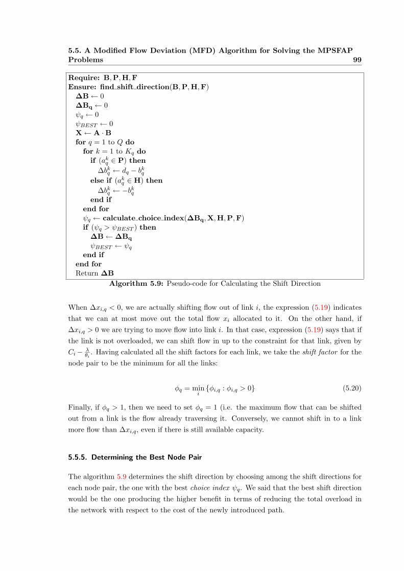
5.5. A Modified Flow Deviation (MFD) Algorithm for Solving the MPSFAPProblems 99
Require: B,P,H,FEnsure: find shift direction(B,P,H,F)
∆B← 0∆Bq ← 0ψq ← 0ψBEST ← 0X← A ·Bfor q = 1 to Q do
for k = 1 to Kq doif (akq ∈ P) then
∆bkq ← dq − bkqelse if (akq ∈ H) then
∆bkq ← −bkqend if
end forψq ← calculate choice index(∆Bq,X,H,P,F)if (ψq > ψBEST ) then
∆B←∆Bq
ψBEST ← ψqend if
end forReturn ∆B
Algorithm 5.9: Pseudo-code for Calculating the Shift Direction
When ∆xi,q < 0, we are actually shifting flow out of link i, the expression (5.19) indicatesthat we can at most move out the total flow xi allocated to it. On the other hand, if∆xi,q > 0 we are trying to move flow into link i. In that case, expression (5.19) says that ifthe link is not overloaded, we can shift flow in up to the constraint for that link, given byCi− λ
θi. Having calculated all the shift factors for each link, we take the shift factor for the
node pair to be the minimum for all the links:
φq = mini{φi,q : φi,q > 0} (5.20)
Finally, if φq > 1, then we need to set φq = 1 (i.e. the maximum flow that can be shiftedout from a link is the flow already traversing it. Conversely, we cannot shift in to a linkmore flow than ∆xi,q, even if there is still available capacity.
5.5.5. Determining the Best Node Pair
The algorithm 5.9 determines the shift direction by choosing among the shift directions foreach node pair, the one with the best choice index ψq. We said that the best shift directionwould be the one producing the higher benefit in terms of reducing the total overload inthe network with respect to the cost of the newly introduced path.

1005. Contribution to the Development of Heuristics for Solving the Minimum
Path Set and Flow Allocation Problems (MPSFAP)
Require: ∆B,X {called with ∆B calculates φ, called with ∆Bq calculates φq}Ensure: find shift factor(∆B,X)φq ← 0φi,q ← 0for q = 1 to Q do
∆Xq ← A ·∆Bq
for i = 1 to M doif (∆xi,q < 0) thenφi,q ← xi
|∆xi,q |else if (∆xi,q > 0) and (xi < Ci − λ
θi) then
φi,q ←Ci− λ
θi−xi
∆xi,q
end ifif (φi,q > 0) and (φi,q < φq) thenφq ← φi,q
end ifend for
end forif (φq > 1) thenφq ← 1
end ifReturn φq
Algorithm 5.10: Pseudo-code for Calculating the Shift Factor
We calculate then a choice index for every pair of nodes as follows:
ψq =
φq
∑Mi=1 γi|∆xi,q |Fq
if γi = 1 for some i|∆xi,q |Fq
if γi = 0 for all i ∧ φq ≥ 1
0 otherwise
(5.21)
where γi = 0 if link i is not overloaded (xi > Ci − λθi
) and 1 if the link is overloaded.Fq =
∑Kq
k=1 hkqF
kq (i.e. the sum of all used paths in the current iteration). ψq is actually
measuring the amount of reduction on the overloaded links relative to the cost of the setof used paths for a given node pair q, including the paths added in the current iteration (ifsome path is added). If there are no overloaded links, we allow the algorithm to try andrearrange the path flows to see if there is any place for flow aggregation. We add this possi-bility in the second option in (5.21): flow aggregation will only be possible if the shift factorfor the candidate node pair is 1 or greater, since the flow would be further splitted otherwise.
Finally, the MFD algorithm can be also adapted to solve the MPSFAP2 problems. Simplychanging the evaluation of the weights for each path during the algorithm to:

5.5. A Modified Flow Deviation (MFD) Algorithm for Solving the MPSFAPProblems 101
Require: ∆Bq,X,H,P,FEnsure: calculate choice index(∆Bq,X,H,P,F)ψq1, ψq2, ψq, ψBEST ← 0φq ← 0overload← NOfor q = 1 to Q doφq ← find shift factor(∆Bq,X)for i = 1 to M do
∆Xq ← A ·∆Bq
if (xi > Ci − λθi
) thenψq1 ← ψq1 + φq|∆xi,q|overload← YES
else if (φq ≥ 1) and (|∆xi,q| > 0) thenψq2 ← |∆xi,q|
end ifend forif (overloaded = YES) thenψq ← ψq1
elseψq ← ψq2
end iffor all akq ∈ H ∪P doFq ← Fq + F kq
end forψq ← ψq
Fq
if (ψq > ψBEST ) thenψBEST ← ψq
end ifend forReturn ψBEST
Algorithm 5.11: Pseudo-code for Calculating the Choice Index
F kq = wkq + hkq
M∑i=1
akq,iλ
Ci − xi+
M∑i=1
akq,if(xi) (5.22)
with f(xi) defined as in (5.15). This way of calculating the path weights consider thepath delay as part of its length. Since only the equation (5.15) has been considered in ourimplementation for calculating the path weights, we restrain ourselves to the an analysis ofthe results obtained from the MFD algorithm for the MPSFAP1 problems.
5.5.6. Evaluation of the MFD Algorithm for MPSFAP
As with the TS heuristics in Section 5.3.4, we run the MFD algorithm for the same set of 25matrixes, and network topologies NET1 and NET2. We then compare the results obtained
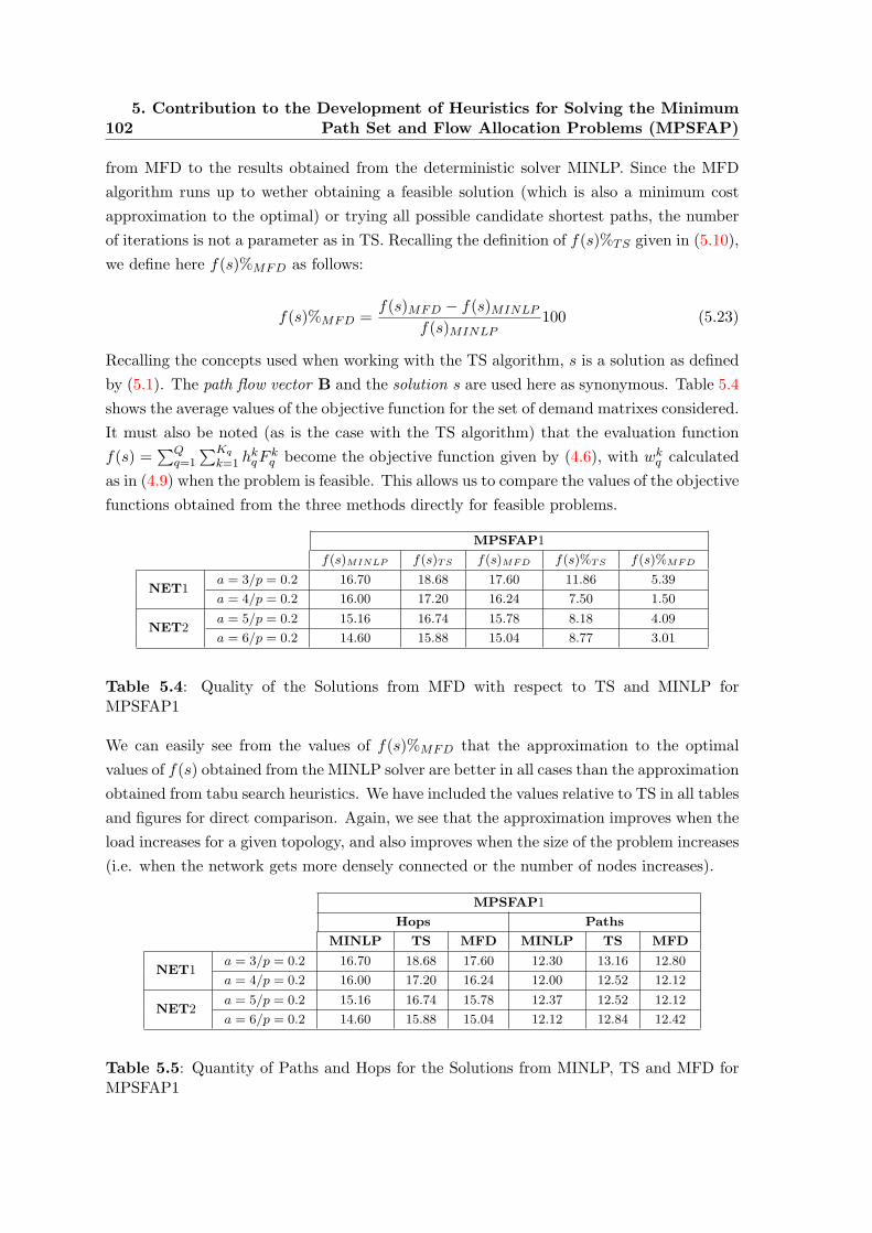
1025. Contribution to the Development of Heuristics for Solving the Minimum
Path Set and Flow Allocation Problems (MPSFAP)
from MFD to the results obtained from the deterministic solver MINLP. Since the MFDalgorithm runs up to wether obtaining a feasible solution (which is also a minimum costapproximation to the optimal) or trying all possible candidate shortest paths, the numberof iterations is not a parameter as in TS. Recalling the definition of f(s)%TS given in (5.10),we define here f(s)%MFD as follows:
f(s)%MFD =f(s)MFD − f(s)MINLP
f(s)MINLP100 (5.23)
Recalling the concepts used when working with the TS algorithm, s is a solution as definedby (5.1). The path flow vector B and the solution s are used here as synonymous. Table 5.4shows the average values of the objective function for the set of demand matrixes considered.It must also be noted (as is the case with the TS algorithm) that the evaluation functionf(s) =
∑Qq=1
∑Kq
k=1 hkqF
kq become the objective function given by (4.6), with wkq calculated
as in (4.9) when the problem is feasible. This allows us to compare the values of the objectivefunctions obtained from the three methods directly for feasible problems.
MPSFAP1
f(s)MINLP f(s)TS f(s)MFD f(s)%TS f(s)%MFD
NET1a = 3/p = 0.2 16.70 18.68 17.60 11.86 5.39
a = 4/p = 0.2 16.00 17.20 16.24 7.50 1.50
NET2a = 5/p = 0.2 15.16 16.74 15.78 8.18 4.09
a = 6/p = 0.2 14.60 15.88 15.04 8.77 3.01
Table 5.4: Quality of the Solutions from MFD with respect to TS and MINLP forMPSFAP1
We can easily see from the values of f(s)%MFD that the approximation to the optimalvalues of f(s) obtained from the MINLP solver are better in all cases than the approximationobtained from tabu search heuristics. We have included the values relative to TS in all tablesand figures for direct comparison. Again, we see that the approximation improves when theload increases for a given topology, and also improves when the size of the problem increases(i.e. when the network gets more densely connected or the number of nodes increases).
MPSFAP1
Hops Paths
MINLP TS MFD MINLP TS MFD
NET1a = 3/p = 0.2 16.70 18.68 17.60 12.30 13.16 12.80
a = 4/p = 0.2 16.00 17.20 16.24 12.00 12.52 12.12
NET2a = 5/p = 0.2 15.16 16.74 15.78 12.37 12.52 12.12
a = 6/p = 0.2 14.60 15.88 15.04 12.12 12.84 12.42
Table 5.5: Quantity of Paths and Hops for the Solutions from MINLP, TS and MFD forMPSFAP1

5.5. A Modified Flow Deviation (MFD) Algorithm for Solving the MPSFAPProblems 103
NET1 (a=3/p=0.2)
10,00
12,00
14,00
16,00
18,00
20,00
22,00
24,00
26,00
28,00
30,00
1 2 3 4 5 6 7 8 9 10 11 12 13 14 15 16 17 18 19 20 21 22 23 24 25Matrix
Hop
s
Hops - MPSFAP1 (NEOS)
Hops - MPSFAP1 (TS)
Hops - MPSFAP1 (MFD)
(a) Hops, a = 3
NET1 (a=3/p=0.2)
10,00
11,00
12,00
13,00
14,00
15,00
16,00
17,00
18,00
19,00
20,00
1 2 3 4 5 6 7 8 9 10 11 12 13 14 15 16 17 18 19 20 21 22 23 24 25Matrix
Path
s
Paths - MPSFAP1 (NEOS)
Paths - MPSFAP1 (TS)
Paths - MPSFAP1 (MFD)
(b) Paths, a = 3
NET1 (a=4/p=0.2)
10,00
12,00
14,00
16,00
18,00
20,00
22,00
24,00
26,00
28,00
30,00
1 2 3 4 5 6 7 8 9 10 11 12 13 14 15 16 17 18 19 20 21 22 23 24 25Matrix
Hop
s
Hops - MPSFAP1 (NEOS)
Hops - MPSFAP1 (TS)
Hops - MPSFAP1 (MFD)
(c) Hops, a = 4
NET1 (a=4/p=0.2)
10,00
11,00
12,00
13,00
14,00
15,00
16,00
17,00
18,00
19,00
20,00
1 2 3 4 5 6 7 8 9 10 11 12 13 14 15 16 17 18 19 20 21 22 23 24 25Matrix
Path
s
Paths - MPSFAP1 (NEOS)
Paths - MPSFAP1 (TS)
Paths - MPSFAP1 (MFD)
(d) Paths, a = 4
Figure 5.5: Results from MINLP Solver (NEOS), Tabu Search (TS) and Modified FlowDeviation (MFD) for NET1
Here again, as the problem size increases, a larger number of node pairs will appear ascandidates for becoming a shift direction, as there will be more paths available connectingeach node pair and more node pairs to consider. It can be observed as well that, comparedto the values obtained from MINLP solver for MTDFAP problem (the one minimizing thetotal delay of used paths in the network), the MFD algorithm always constitutes an im-provement on the proposed objectives: to obtain layouts minimizing the total number ofhops (and indirectly of paths) in the layout. Figures 5.5 and 5.6 show the number of hopsand paths obtained from the three methods for NET1 and NET2 respectively. For almostall matrixes, the TS algorithm constitutes an upper bound for the number of hops and pathsobtained from the MFD algorithm. Finally, CPU times required by MFD under the sameconditions than TS are under the second for both topologies, already ten times less thantimes consumed by TS.

1045. Contribution to the Development of Heuristics for Solving the Minimum
Path Set and Flow Allocation Problems (MPSFAP)
NET2 (a=5/p=0.2)
10,00
12,00
14,00
16,00
18,00
20,00
22,00
24,00
26,00
28,00
30,00
1 2 3 4 5 6 7 8 9 10 11 12 13 14 15 16 17 18 19 20 21 22 23 24 25Matrix
Hop
s
Hops - MPSFAP1 (NEOS)
Hops - MPSFAP1 (TS)
Hops - MPSFAP1 (MFD)
(a) Hops, a = 5
NET2 (a=5/p=0.2)
10,00
11,00
12,00
13,00
14,00
15,00
16,00
17,00
18,00
19,00
20,00
1 2 3 4 5 6 7 8 9 10 11 12 13 14 15 16 17 18 19 20 21 22 23 24 25Matrix
Path
s
Paths - MPSFAP1 (NEOS)
Paths - MPSFAP1 (TS)
Paths - MPSFAP1 (MFD)
(b) Paths, a = 5
NET2 (a=6/p=0.2)
10,00
12,00
14,00
16,00
18,00
20,00
22,00
24,00
26,00
28,00
30,00
1 2 3 4 5 6 7 8 9 10 11 12 13 14 15 16 17 18 19 20 21 22 23 24 25Matrix
Hop
s
Hops - MPSFAP1 (NEOS)
Hops - MPSFAP1 (TS)
Hops - MPSFAP1 (MFD)
(c) Hops, a = 6
NET2 (a=6/p=0.2)
10,00
11,00
12,00
13,00
14,00
15,00
16,00
17,00
18,00
19,00
20,00
1 2 3 4 5 6 7 8 9 10 11 12 13 14 15 16 17 18 19 20 21 22 23 24 25Matrix
Path
s
Paths - MPSFAP1 (NEOS)
Paths - MPSFAP1 (TS)
Paths - MPSFAP1 (MFD)
(d) Paths, a = 6
Figure 5.6: Results from MINLP Solver (NEOS), Tabu Search (TS) and Modified FlowDeviation (MFD) for NET2
In next Chapter we compare results obtained from both MFD and TS for two large topolo-gies obtained from real-life size networks. This results allow us to analyze the behavior ofthe described heuristics as well as the pertinence and applicability of each one to day-to-dayoperational environment.
5.6. Conclusions
In the previous Chapter we have shown the interest, from an operator’s standpoint, ofconsidering complexity objectives when designing optimal MPLS layouts. In the presentChapter the major contribution consist in the definition and implementation of two heuris-tic methods to deal with the MPSFAP problems. The first heuristic is a generic heuristicusing Tabu Search (TS) methods and particular evaluation of the generated solution toexplore the solution space. The second heuristic is an ad-hoc heuristic which makes use of

5.6. Conclusions 105
the particular structure and nature of the problem to intelligently search the solution spacerather than randomly. This last heuristics is based on a modification to the general proce-dure of the well known Flow Deviation Method to solve the multicommodity flow problemfor convex objective functions. The resulting algorithm is referred as MFD (Modified FlowDeviation) algorithm. Results obtained with both heuristic methods are compared to thesolutions obtained using the deterministic solver available for the MINLP problems, in orderto establish the quality of the solutions obtained through heuristics methods with respect tothe optimal solution. Due to problem size limitations when using the deterministic solvers,results are compared for small topologies in order to obtain some insight in the behaviorof the heuristics. Results for the MTDFAP problem are also given as a reference. Finallyresults obtained with the TS and the MFD heuristics are compared one to another in orderto establish the relative quality of the solutions obtained through both methods.
Results show that both, TS and MFD yield fairly good approximations for small networktopologies. MFD however, shows better quality results with respect to those obtained byusing the TS algorithm. Besides, the execution times on a standard personal computerare far lower for MFD than for TS. The figures obtained for small networks encourage usto continue further exploring both heuristic methods, which we do in the next Chapter.Although small network topologies do not offer much space for a real difference among thevarious optimization criteria, we can already see that we obtain layouts for the MPSFAPobjective functions using less hops and consequently less paths than those obtained forMTDFAP objectives (i.e. the classic performance objectives used extensively through theliterature). In next Chapter we evaluate both heuristic methods for two large networktopologies, and we explore the results in order to obtain more insight in the behavior of thecost functions proposed, as well as to evaluate the performance of the heuristic methodsdeveloped.


6. Results and Analysis of the MPSFAP Problems for Large
Networks Using Tabu Search (TS) and Modified Flow
Deviation (MFD) Methods
In the previous Chapter, we have developed two heuristic methods to solve the MPSFAPproblem: a Tabu Search meta-heuristic algorithm based on meta-heuristics, and a ModifiedFlow Deviation algorithm based on the Frank-Wolfe method (ad-hoc heuristics). Thesealgorithms are expected to allow us to overcome the problem size limitations described inChapter 4 when evaluating and validating the proposed model for MPLS layout complexityoptimization through deterministic solvers. In the mentioned Chapter, we have individuallyevaluated each one of the developed heuristics for small network topologies like the onesused to first evaluate the models in Chapter 4. We have concluded that both heuristics arefairly good approximations of the optimal values obtained through the deterministic MINLPsolver. We have also noted that the MFD algorithm outperforms the TS algorithms bothin terms of computational effort and in terms of the quality of the results for the studiedtopologies.
In the present Chapter, we extend the study of both heuristics to large network topologies.Two network topologies are presented, representing national span networks from Europe(France) and United States. Then results for different load situations using both algorithmsfor the presented network topologies are obtained and compared. Finally, based on theresult comparison between the two heuristics, further analysis on results for the MPSFAPproblem using the MFD algorithm are presented.
6.1. Considered Network Topologies
We run the TS and MFD algorithms on two medium-sized to large topologies issued fromreal-life networks, covering a national span, both in Europe and United States. The VTHDnetwork shown in Figure 6.1 is modelled after the French National Research Network, de-ployed in the context of the VTHD (Vraiment Tres Haut Debit)[63] research project, whereonly the core nodes of network are represented. In a similar way, the NSF network shown inFigure 6.2 is a model of the Internet in the US at the time of ARPANET. We have chosenthese two topologies because they represent large networks issued from real-life planning,with medium to high degrees of connectivity (2.66 for VTHD and 3 for NSF) transportingtraffic aggregates.
107
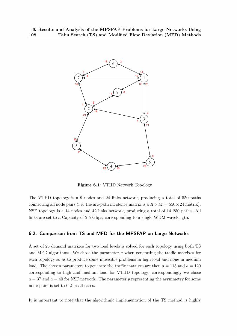
1086. Results and Analysis of the MPSFAP Problems for Large Networks Using
Tabu Search (TS) and Modified Flow Deviation (MFD) Methods
Figure 6.1: VTHD Network Topology
The VTHD topology is a 9 nodes and 24 links network, producing a total of 550 pathsconnecting all node pairs (i.e. the arc-path incidence matrix is a K×M = 550×24 matrix).NSF topology is a 14 nodes and 42 links network, producing a total of 14, 250 paths. Alllinks are set to a Capacity of 2.5 Gbps, corresponding to a single WDM wavelength.
6.2. Comparison from TS and MFD for the MPSFAP on Large Networks
A set of 25 demand matrixes for two load levels is solved for each topology using both TSand MFD algorithms. We chose the parameter a when generating the traffic matrixes foreach topology so as to produce some infeasible problems in high load and none in mediumload. The chosen parameters to generate the traffic matrixes are then a = 115 and a = 120corresponding to high and medium load for VTHD topology; correspondingly we chosea = 37 and a = 40 for NSF network. The parameter p representing the asymmetry for somenode pairs is set to 0.2 in all cases.
It is important to note that the algorithmic implementation of the TS method is highly

6.2. Comparison from TS and MFD for the MPSFAP on Large Networks 109
1
1 2
3
4
5
6
7
810
11
12
14
13
9
2
3
4
5
6
7
8
9
10
11
12
13
14
15
16
17
181920
21
22
23
24
25
26
2728 29
30
31
32
3334
3536
37
38
39
40
41
42
Figure 6.2: NSF Network Topology
memory consuming and computationally intensive. A number of neighbors need to be gen-erated and kept in memory at each iteration, limiting the maximum size of the problemsthat can be given as input (although much larger than for deterministic solvers). At thesame time, a second limitation appears when increasing the number of paths for the sametopology. Indeed, the time consumed to accomplish each iteration of the TS algorithm de-pends directly on the total number of paths in A and the number of neighbors to generate,constituting a practical limitation when running large sets of demand matrixes. Reducingthe number of neighbors to generate at each iteration of the the TS algorithm reduces theprobability of finding a good neighbor, and as such, the quality of the progression in thesolution space. An alternative to reducing the number of neighbors is to reduce the numberof paths considered in the arc-path incidence matrix A. Observing from results in previouschapters, the path multiplicity of the solutions (even for high load levels) is near unity.We observe as well that, as the path weights in the objective function for MPSFAP1 arethe hop counts, the paths used in the solution tend to be the shortest or next to shortestpath connecting each node pair. Providing then a reduced set of paths to the algorithmwould not greatly penalize the quality of the solution if enough alternative paths (chosenin increasing lengths) connecting each node pair are provided. Consequently, we considera reduced arc-path incidence matrix, containing a total of 910 paths (i.e. a set of 5 pathsfor every node pair), as a good trade-off between path candidates and time consumed. It isalso important to note that the algorithmic implementation of the MFD algorithm doesn’tpresent this limitation. In fact, only one instance of the problem is kept in memory at each
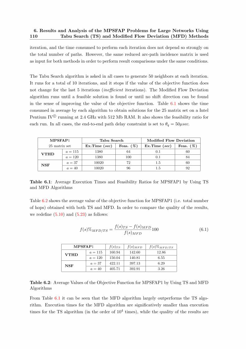
1106. Results and Analysis of the MPSFAP Problems for Large Networks Using
Tabu Search (TS) and Modified Flow Deviation (MFD) Methods
iteration, and the time consumed to perform each iteration does not depend so strongly onthe total number of paths. However, the same reduced arc-path incidence matrix is usedas input for both methods in order to perform result comparisons under the same conditions.
The Tabu Search algorithm is asked in all cases to generate 50 neighbors at each iteration.It runs for a total of 10 iterations, and it stops if the value of the objective function doesnot change for the last 5 iterations (inefficient iterations). The Modified Flow Deviationalgorithm runs until a feasible solution is found or until no shift direction can be foundin the sense of improving the value of the objective function. Table 6.1 shows the timeconsumed in average by each algorithm to obtain solutions for the 25 matrix set on a IntelPentium IV c© running at 2.4 GHz with 512 Mb RAM. It also shows the feasibility ratio foreach run. In all cases, the end-to-end path delay constraint is set to θq = 50µsec.
MPSFAP1 Tabu Search Modified Flow Deviation
25 matrix set Ex.Time (sec) Feas. (%) Ex.Time (sec) Feas. (%)
VTHDa = 115 1380 64 0.1 60
a = 120 1380 100 0.1 84
NSFa = 37 10020 72 1.5 60
a = 40 10020 96 1.5 92
Table 6.1: Average Execution Times and Feasibility Ratios for MPSFAP1 by Using TSand MFD Algorithms
Table 6.2 shows the average value of the objective function for MPSFAP1 (i.e. total numberof hops) obtained with both TS and MFD. In order to compare the quality of the results,we redefine (5.10) and (5.23) as follows:
f(s)%MFD/TS =f(s)TS − f(s)MFD
f(s)MFD100 (6.1)
MPSFAP1 f(s)TS f(s)MFD f(s)%MFD/TS
VTHDa = 115 160.94 142.60 12.86
a = 120 150.04 140.81 6.55
NSFa = 37 422.11 397.13 6.29
a = 40 405.71 392.91 3.26
Table 6.2: Average Values of the Objective Function for MPSFAP1 by Using TS and MFDAlgorithms
From Table 6.1 it can be seen that the MFD algorithm largely outperforms the TS algo-rithm. Execution times for the MFD algorithm are significatively smaller than executiontimes for the TS algorithm (in the order of 104 times), while the quality of the results are

6.2. Comparison from TS and MFD for the MPSFAP on Large Networks 111
significatively better for the MFD algorithm in terms of value of the objective functionunder all load conditions, as it can be observed in the Table 6.2. However, the feasibilityratio is better for the TS algorithm than for the MFD algorithm. This is due mainly to theend-to-end path constraint simplification, which imposes more restrictive constraints to thelink loads. Table 6.3 shows the average quantity of paths and the average maximum end-to-end path delay (τkq ) obtained for MPSFAP1 using TS and MFD algorithms on VTHDand NSF topologies for the two load situations.
MPSFAP1 Tabu Search Modified Flow Deviation
25 matrix set Paths Max. τkq (µsec) Paths Max. τk
q (µsec)
VTHDa = 115 75.38 26.05 72.70 15.89
a = 120 73.28 21.83 71.76 14.27
NSFa = 37 189.06 39.66 183.40 25.65
a = 40 185.46 34.33 182.30 19.23
Table 6.3: Average Paths and Average Maximum End-to-end Path Delay for MPSFAP1by Using TS and MFD Algorithms
Due to the simplification of the end-to-end path delay constraints, more restrictive con-straints are imposed on link loads, resulting in a higher infeasibility ratio. In fact, as wecan see in Table 6.3 and Figure 6.5, the end-to-end path delay on layouts calculated withMFD algorithm are significantly lower than those on layouts calculated with the TS method.More, we verify that resulting path delays with MFD runs are far from the imposed con-straint θq. Increasing then the end-to-end path delay constraints for MFD would allow forhigher feasibility rates without violating the originally set constraints. This possibility isfurther explored in next section.
Figures 6.3 and 6.4 show the detailed hop count (the value of the objective function) andthe quantity of paths used by each layout obtained as a solution by means of TS and MFDto the corresponding demand matrix. We see that in all cases the MFD algorithm obtainslayouts with a lower number of hops and paths than those obtained by the TS algorithm.To increase the quality of the solutions obtained with TS we should increase the numberof iterations over which the algorithm explores the solution space, further increasing thenecessary CPU time. The fact that CPU times required by TS to obtain solutions of com-parable but lower quality than those obtained with MFD are measured in hours instead ofin seconds or minutes, tells us that the algorithm is not compatible with operational times.In fact, if our objective is to adapt the network to changing traffic conditions on a long-termbasis, we should be able to recalculate the layout in less time than the reconfiguration cycle.Having found that the MFD algorithm performs better quality calculations in lower CPUtimes (several orders of magnitude lower), further development of the TS algorithm is no

1126. Results and Analysis of the MPSFAP Problems for Large Networks Using
Tabu Search (TS) and Modified Flow Deviation (MFD) Methods
VTHD a=115/p=0.2
100,00
150,00
200,00
250,00
300,00
350,00
1 2 3 4 5 6 7 8 9 10 11 12 13 14 15 16 17 18 19 20 21 22 23 24 25Matrix
Hop
s
Hops - TSHops - MFD
(a) VTHD, a = 115
VTHD a=120/p=0.2
100,00
120,00
140,00
160,00
180,00
200,00
220,00
240,00
260,00
280,00
1 2 3 4 5 6 7 8 9 10 11 12 13 14 15 16 17 18 19 20 21 22 23 24 25Matrix
Hop
s
Hops - TSHops - MFD
(b) VTHD, a = 120
NSF a=37/p=0.2
300,00
350,00
400,00
450,00
500,00
550,00
1 2 3 4 5 6 7 8 9 10 11 12 13 14 15 16 17 18 19 20 21 22 23 24 25Matrix
Hop
s
Hops - TSHops - MFD
(c) NSF, a = 37
NSF a=40/p=0.2
300,00
350,00
400,00
450,00
500,00
550,00
1 2 3 4 5 6 7 8 9 10 11 12 13 14 15 16 17 18 19 20 21 22 23 24 25Matrix
Hop
s
Hops - TSHops - MFD
(d) NSF, a = 40
Figure 6.3: Value of The Objective Function for MPSFAP1 (Total Hops) for VTHD andNSF Network Topologies using TS and MFD Algorithms
longer justified for solving the reconfiguration problem defined in next Chapter.
Regarding the behavior of the objective function we note that, as it is expected, MPSFAP1requires more paths (and in consequence more hops) under heavy load conditions than itdoes under medium load conditions. Indeed, as the demand levels increase, the traffic needto be splitted among the available paths in order to be able to absorb the demand. Further,it can be observed that MPSFAP1 objective keeps a low number of required paths overall.Since VTHD topology is a 9 node network, the total number of node pairs is N(N−1) = 72,while for NSF the total is 182 pairs. We see from Table 6.3 that the average required num-ber of paths for VTHD by MFD algorithm is 72.70 under heavy load and 71.76 under lightload. This means that in average, solutions obtained for MPSFAP1 for VTHD are using lessthan 1 extra path under heavy load to transport the whole demand (under medium load theaverage number of required paths is less than 72 because on some demand matrixes there

6.2. Comparison from TS and MFD for the MPSFAP on Large Networks 113
VTHD a=115/p=0.2
65,00
70,00
75,00
80,00
85,00
90,00
95,00
100,00
105,00
110,00
1 2 3 4 5 6 7 8 9 10 11 12 13 14 15 16 17 18 19 20 21 22 23 24 25Matrix
Path
s
Hops - TSHops - MFD
(a) VTHD, a = 115
VTHD a=120/p=0.2
60,00
65,00
70,00
75,00
80,00
85,00
90,00
95,00
100,00
105,00
110,00
1 2 3 4 5 6 7 8 9 10 11 12 13 14 15 16 17 18 19 20 21 22 23 24 25Matrix
Path
s
Hops - TSHops - MFD
(b) VTHD, a = 120
NSF a=37/p=0.2
150,00
160,00
170,00
180,00
190,00
200,00
210,00
220,00
1 2 3 4 5 6 7 8 9 10 11 12 13 14 15 16 17 18 19 20 21 22 23 24 25Matrix
Path
s
Hops - TSHops - MFD
(c) NSF, a = 37
NSF a=40/p=0.2
150,00
160,00
170,00
180,00
190,00
200,00
210,00
220,00
1 2 3 4 5 6 7 8 9 10 11 12 13 14 15 16 17 18 19 20 21 22 23 24 25Matrix
Path
s
Hops - TSHops - MFD
(d) NSF, a = 40
Figure 6.4: Used Paths for Layouts Obtained from MPSFAP1 for VTHD and NSF NetworkTopologies using TS and MFD Algorithms
are nodes with 0 demand). In the case of NSF, less than 2 extra paths were required to routethe whole demand under heavy load, while less than 1 extra path is necessary under mediumload. The average hop-count for VTHD is 1.96, while for NSF is 2.16. These figures areclose to the single-path routing case, leading us to think that the optimal layouts accordingto MPSFAP1 could be built using an IGP protocol in a pure IP environment. However, tofind a unique IGP metric compatible with the optimal general-routing problem (studied in[40]) seems particularly difficult. Alternatives using a mix of IGP metrics for the compat-ible part of the optimal layout and complementary LSPs to complete it have been proposed.
Finally, paying attention to the individual maximum end-to-end path delay in Figure 6.5,we see that they do not largely depend on the load level. This is explained by the fact that,as the MPSFAP1 objective is to minimize the number of hops (consequently of paths) usedin the layout, as far as there is some room in the links, the traffic will be aggregated up

1146. Results and Analysis of the MPSFAP Problems for Large Networks Using
Tabu Search (TS) and Modified Flow Deviation (MFD) Methods
VTHD a=115/p=0.2
0,00
10,00
20,00
30,00
40,00
50,00
60,00
1 2 3 4 5 6 7 8 9 10 11 12 13 14 15 16 17 18 19 20 21 22 23 24 25Matrix
Max
.Pat
h D
elay
(mic
rose
cond
s)
Max. Path Delay - TSMax. Path Delay - MFD
(a) VTHD, a = 115
VTHD a=120/p=0.2
0,00
10,00
20,00
30,00
40,00
50,00
60,00
1 2 3 4 5 6 7 8 9 10 11 12 13 14 15 16 17 18 19 20 21 22 23 24 25Matrix
Max
. Pat
h D
elay
(mic
rose
cond
s)
Max. Path Delay - TSMax. Path Delay - MFD
(b) VTHD, a = 120
NSF a=37/p=0.2
0,00
10,00
20,00
30,00
40,00
50,00
60,00
1 2 3 4 5 6 7 8 9 10 11 12 13 14 15 16 17 18 19 20 21 22 23 24 25Matrix
Max
.Pat
h D
elay
(mic
rose
cond
s)
Max. Path Delay - TSMax. Path Delay - MFD
(c) NSF, a = 37
NSF a=40/p=0.2
0,00
10,00
20,00
30,00
40,00
50,00
60,00
1 2 3 4 5 6 7 8 9 10 11 12 13 14 15 16 17 18 19 20 21 22 23 24 25Matrix
Max
.Pat
h D
elay
(mic
rose
cond
s)
Max. Path Delay - TSMax. Path Delay - MFD
(d) NSF, a = 40
Figure 6.5: Maximum Path Delay in Layouts Obtained from MPSFAP1 for VTHD andNSF Network Topologies using TS and MFD Algorithms
to the limit imposed by the capacity and path delay constraints. As the results show, theminimum set of paths is obtained to the expense of growing end-to-end path delays, provingthat the introduced constraints are key to keeping the intended QoS guarantees.
In next section we further analyze results for the VTHD and NSF topologies using the MFDalgorithm, as the running times and quality of the obtained results as shown in the presentsection allow for extensive tests to gain insight in the behavior of the dimensioning problemon large networks.
6.3. Result Analysis of Large Networks by Using MFD
Given the observed performance of the MFD algorithm as established in previous section,we further analyze some results obtained for the VTHD and NSF networks. For the two

6.3. Result Analysis of Large Networks by Using MFD 115
values of the parameter a in the traffic matrixes, corresponding to high and medium loadlevels for each network, we explore results obtained when varying the end-to-end pathdelay constraint θq for every node pair. The tightest value is set to 50 µseconds, and theconstraint is relaxed up to 170 µseconds. The feasibility ratio, and the evolution of theobserved number of hops and paths, as well as the evolution of the average maximum andabsolute maximum end-to-end path delay with respect to the changes in the constraints areanalyzed. For simplicity, the path delay constraints are all set to the same value.
VTHD (a=115/p=0.2)
10,00
15,00
20,00
25,00
30,00
35,00
40,00
45,00
50,00
55,00
60,00
50 60 70 80 90 100 110 120 130 140 150 160 170Max. Path Delay Constraint (microseconds)
mic
rose
cond
s
Max. Path Delay (Average)Max. Path Delay (Max)
Original Path-Delay Constraint (50 microseconds)
(a) VTHD, a = 115
VTHD (a=120/p=0.2)
10,00
15,00
20,00
25,00
30,00
35,00
40,00
45,00
50,00
55,00
60,00
50 60 70 80 90 100 110 120 130 140 150 160 170Max. Path Delay Constraint (microseconds)
mic
rose
cond
s
Max. Path Delay (Average)Max. Path Delay (Max)
Original Path-Delay Constraint (50 microseconds)
(b) VTHD, a = 120
Figure 6.6: Maximum Path Delay and Average Maximum Path Delay for VTHD NetworkTopologies Using MFD Algorithm, as a Function of Delay Constraint
NSF (a=37/p=0.2)
10,00
20,00
30,00
40,00
50,00
60,00
70,00
50 60 70 80 90 100 110 120 130 140 150 160 170Max. Path Delay Constraint (microseconds)
mic
rose
cond
s
Max. Path Delay (Average)Max. Path Delay (Max)
Original Path-Delay Constraint (50 microseconds)
(a) NSF, a = 37
NSF (a=40/p=0.2)
10,00
20,00
30,00
40,00
50,00
60,00
70,00
50 60 70 80 90 100 110 120 130 140 150 160 170Max. Path Delay Constraint (microseconds)
mic
rose
cond
s
Max. Path Delay (Average)Max. Path Delay (Max)
Original Path-Delay Constraint (50 microseconds)
(b) NSF, a = 40
Figure 6.7: Maximum Path Delay and Average Maximum Path Delay for NSF NetworkTopologies Using MFD Algorithm, as a Function of Delay Constraint
Figures 6.6 and 6.7 show the evolution of the end-to-end path delay with the constraintimposed on the maximum allowable end-to-end path delays for both topologies. As ithas been highlighted in section 6.2, when setting the end-to-end path delay constraint to

1166. Results and Analysis of the MPSFAP Problems for Large Networks Using
Tabu Search (TS) and Modified Flow Deviation (MFD) Methods
50 µseconds, the observed absolute maximum end-to-end path delay (i.e. the maximumobserved among all the paths in the layouts obtained for the set of 25 traffic matrixes fora given load level and θq) is far lower than the value imposed by the constraint. This isdue to the way those constraints were simplified in order to be able to calculate flow shiftsfor the MFD algorithm in a link-by-link basis taking into account the path flows traversingeach link. A factor to analyze is then how the absolute maximum path delay for any pathin the layout relates to the imposed path delay constraint.
VTHD (a=115/p=0.2)
140,00
140,50
141,00
141,50
142,00
142,50
143,00
50 60 70 80 90 100 110 120 130 140 150 160 170Max. Path Delay Constraint (microseconds)
Avg
. Hop
s
Avg. Hops
(a) VTHD, a = 115
VTHD (a=120/p=0.2)
140,00
140,50
141,00
141,50
142,00
142,50
143,00
50 60 70 80 90 100 110 120 130 140 150 160 170Max. Path Delay Constraint (microseconds)
Avg
. Hop
s
Avg. Hops
(b) VTHD, a = 120
Figure 6.8: Average Quantity of Hops for VTHD Network Topologies Using MFD Algo-rithm, as a Function of Delay Constraint
NSF (a=37/p=0.2)
390,00
400,00
50 60 70 80 90 100 110 120 130 140 150 160 170Max. Path Delay Constraint (microseconds)
Avg
. Hop
s
Avg. Hops
(a) NSF, a = 37
NSF (a=40/p=0.2)
390,00
400,00
50 60 70 80 90 100 110 120 130 140 150 160 170Max. Path Delay Constraint (microseconds)
Avg
. Hop
s
Avg. Hops
(b) NSF, a = 40
Figure 6.9: Average Quantity of Hops for NSF Network Topologies Using MFD Algorithm,as a Function of Delay Constraint
As we would expect, the maximum path delay (maxk,q{τkq}) obtained in any path of the
calculated layout increases as the path delay constraint (θq) are made less tight. We seethat, even when increasing θq to 160 µseconds for a high load situation, maxk,q
{τkq}
stays

6.3. Result Analysis of Large Networks by Using MFD 117
below the originally set constraint of 50 µseconds. For a medium load situation (a = 120for VTHD and a = 40 for NSF), the maxk,q
{τkq}
reach later the limit imposed by theoriginally set constrain. We can also observe that for NSF network, the maxk,q
{τkq}
crossesthe originally set constraint of 50 µseconds for lower values of the path delay constraintthan it does for VTHD network.
VTHD (a=115/p=0.2)
71,00
71,50
72,00
72,50
73,00
50 60 70 80 90 100 110 120 130 140 150 160 170Max. Path Delay Constraint (microseconds)
Avg
. Pat
hs
Avg. Paths
(a) VTHD, a = 115
VTHD (a=120/p=0.2)
71,00
71,50
72,00
72,50
73,00
50 60 70 80 90 100 110 120 130 140 150 160 170Max. Path Delay Constraint (microseconds)
Avg
. Pat
hs
Avg. Paths
(b) VTHD, a = 120
Figure 6.10: Average Quantity of Paths for VTHD Network Topologies Using MFD Al-gorithm, as a Function of Delay Constraint
NSF (a=37/p=0.2)
180,00
182,00
184,00
50 60 70 80 90 100 110 120 130 140 150 160 170Max. Path Delay Constraint (microseconds)
Avg
. Pat
hs
Avg. Paths
(a) NSF, a = 37
NSF (a=40/p=0.2)
180,00
182,00
184,00
50 60 70 80 90 100 110 120 130 140 150 160 170Max. Path Delay Constraint (microseconds)
Avg
. Pat
hs
Avg. Paths
(b) NSF, a = 40
Figure 6.11: Average Quantity of Paths for NSF Network Topologies Using MFD Algo-rithm, as a Function of Delay Constraint
This can be explained by the fact that the average path length for NSF network is largerthan the average path length for VTHD network. The fact that the obtained path delays arealways lower than the imposed constraints allows us to set less tight constraints, allowing theconcentration of traffic in less paths, and consequently lowering the number of required hops(and indirectly of paths), as it can be seen in Figures 6.8, 6.10, 6.9 and 6.11. This results

1186. Results and Analysis of the MPSFAP Problems for Large Networks Using
Tabu Search (TS) and Modified Flow Deviation (MFD) Methods
in an further improvement on the quality of the results, without violating the originallyset constraints. Further study to find a relationship between the values obtained for thepath delays for a given set of path delay constraints may help to set engineering rulesfor the design of MPLS layouts. This relationship depends on the topology so an explicitrelationship would be difficult to establish, although we see from the figures that a linearfunction yields a fairly good approximation.
VTHD (a=115/p=0.2)
0,00%
10,00%
20,00%
30,00%
40,00%
50,00%
60,00%
70,00%
80,00%
90,00%
100,00%
50 60 70 80 90 100 110 120 130 140 150 160 170Max. Path Delay Constraint (microseconds)
Avg
. Pat
hs
Feasibility (%)
(a) VTHD, a = 115
VTHD (a=120/p=0.2)
0,00%
10,00%
20,00%
30,00%
40,00%
50,00%
60,00%
70,00%
80,00%
90,00%
100,00%
50 60 70 80 90 100 110 120 130 140 150 160 170Max. Path Delay Constraint (microseconds)
Avg
. Pat
hs
Feasibility (%)
(b) VTHD, a = 120
Figure 6.12: Feasibility Rate for VTHD Network Topologies Using MFD Algorithm, as aFunction of Delay Constraint
NSF (a=37/p=0.2)
0,00%
10,00%
20,00%
30,00%
40,00%
50,00%
60,00%
70,00%
80,00%
90,00%
100,00%
50 60 70 80 90 100 110 120 130 140 150 160 170Max. Path Delay Constraint (microseconds)
Avg
. Pat
hs
Feasibility (%)
(a) NSF, a = 37
NSF (a=40/p=0.2)
0,00%
20,00%
40,00%
60,00%
80,00%
100,00%
50 60 70 80 90 100 110 120 130 140 150 160 170Max. Path Delay Constraint (microseconds)
Avg
. Pat
hs
Feasibility (%)
(b) NSF, a = 40
Figure 6.13: Feasibility Rate for NSF Network Topologies Using MFD Algorithm, as aFunction of Delay Constraint
Finally, looking at the feasibility ratios in Figure 6.12 and 6.13, as we would expect, it canbe seen that they improve when the path delay constraints are made less tight. The reasonwhy this happens is simple: as the path delay constraints are relaxed, the allowed reducedcapacity on each link increases, also increasing the total available capacity in the network,

6.4. Conclusions 119
so that traffic matrixes that were infeasible before now become feasible.
6.4. Conclusions
In previous Chapter we developed two heuristic methods to solve the MPSFAP problem.We also tested implementations of both heuristics on small network topologies in order toevaluate the quality of the results obtained, given the problem size limitations imposed bythe deterministic solvers. From results obtained in Chapter 5 we conclude that the TS andMFD algorithms implementing generic and ad-hoc heuristics respectively yield approximateresults within an acceptable tolerance from the optimal solutions. In the present Chapter,we explore the behavior of both algorithms and the cost functions proposed on large net-work topologies. Results are obtained for two load levels, corresponding to heavy and mildload in the network.
Regarding the performance of the algorithms proposed in previous Chapter, for the sametopologies and under the same load conditions, we observe that the MFD algorithm per-forms better than the TS algorithm for both aspects, quality of the solution and executiontime. With respect to the quality of the solutions obtained my MFD, it can be observedthat the value of the MPSFAP1 cost function is lower in all cases, meaning that a lowernumber of hops and paths are used in average. On the other hand, we observe that MFDhas an infeasibility ratio which is higher than the one observed for TS. This is explainedby the fact that the simplification operated on the end-to-end path delay constraint whenimplementing the MFD algorithm imposes more restrictive limitations to the usable capac-ity on the individual links than the TS algorithm. This can be observed when comparingthe maximum end-to-end path delay obtained from both algorithms for each one of the 25traffic matrixes in the test set for any load level. While the maximum path delay valuesobtained with TS are almost always close to the imposed constraint, the values for theMFD algorithm are always far from such limit. This drives us to further explore solutionswith the MFD algorithm for less restrictive path delay constraints, which we do in thesecond part of this Chapter. Further, with respect to execution times, we can observe thatMFD algorithm always find better quality solutions than TS in dramatically lower timesthan TS, due to the inexpensive nature of the operations performed over only a few pathson each iteration of the MFD. The execution times observed with the MFD algorithm arecompatible with an on-line operation of a close control loop, allowing us to reduce the timerequired to calculate optimal layouts and to dimension the network at shorter timescales.However, it is not practical to recalculate the optimal layout in a large network too manytimes too often, since TE mechanisms at shortest timescales applied on local scopes candeal appropriately with the dynamic adaptation needed for the observed variations at thosetimescales, instead of resorting to global changes which are not justified in terms of costs

1206. Results and Analysis of the MPSFAP Problems for Large Networks Using
Tabu Search (TS) and Modified Flow Deviation (MFD) Methods
for the operator. The quality of the observed results, together with the execution times arekey factors, which determined us to further develop the MFD algorithm in future researchdirections, leaving the TS algorithm behind. In particular, a version of the MFD algorithmis adapted to solve the MRPSFAP problem in Chapter 8.
Regarding the behavior of the proposed MPSFAP cost function, the study of results ob-tained by using the MFD algorithm on large network topologies show that when imposingless restrictive constraints under any load condition, the average quantity of hops (and indi-rectly the average quantity of paths) gets further reduced. As expected, reducing the loadconditions on a given network topology, also reduces the number of required hops and pathsfor a given traffic matrix. It is important to note that in all cases the path multiplicityrequired to connect any node pair when calculating the layouts with MPSFAP1 objectiveis close to 1, showing the interest of the proposed cost function as representative of the costobjectives for layout optimization from an operational point of view.

7. Contribution to Reconfiguring MPLS Networks: Design of
Reduced Reconfiguration and Complexity Layouts
7.1. Motivations and Previous Work
In Chapter 4 the problem of dimensioning an MPLS layout has been addressed. Given atraffic demand and a physical network topology, the objective is to find the set of sourcerouted paths and the corresponding flow allocation that minimizes the cost of operation.We have considered so far that the traffic demand is known (e.g. by means of measurementand inference from those measures) and that we want to obtain a unique optimal layout forthat traffic matrix. In this context, we consider that the cost of operation is related to thelayout complexity in terms of quantity of hops and paths that have to be established andmaintained by the operating system. The dimensioning problem is then formulated as amixed-integer non-linear constrained multicommodity flow allocation problem (MPSFAP)including cost functions taking into account the above mentioned cost issues [16].
On long timescales, traffic demands are observed to present systematic long-term trafficvariations on a daily basis [68, 69]. The design of an optimal layout for a given traffic ma-trix constitutes then a point of operation during the periods where the traffic is identified tobe static with respect to the considered timescale. Small traffic variations during this cyclewould be accommodated by TE mechanisms taking action at shorter timescales. However,when the traffic matrix presents significant changes (as those produced when passing fromthe current static period to the next one), the currently operational layout is not able tohandle the new traffic conditions efficiently anymore and has to be recalculated. In thepresent chapter we consider that there is an additional cost for the network operation andmaintenance in reconfiguring the network to the new layout. Indeed, depending on therouting policy being implemented, whether additional resources have to be made availableor service disruption times have to be accepted in order to manage the transition from thecurrent layout to the next one. In this context, the layout has to be recalculated to be op-timal with respect to the layout complexity (in the sense of MPSFAP problems) and withrespect to the reconfiguration complexity.
Reconfiguration studies have been carried out mainly in the context of WDM layouts [25,70, 71] and joint MPLS and WDM layout optimization [72], as well as in the field of generaloptimal routing [73]. Objective functions considered in off-line approaches minimize the
121

1227. Contribution to Reconfiguring MPLS Networks: Design of Reduced
Reconfiguration and Complexity Layouts
number of lightpath additions and deletions [25] or a trade-off among the reconfigurationand the other objectives in the layout design, without considering QoS constraints. In[25] a new virtual topology is obtained by choosing the layout which minimizes the totalnumber of added or deleted lightpaths among all the possible layouts. An optimal layoutis calculated for the old and new demand matrixes. The value of the objective function forthe new layout is then included in a new formulation of the problem for the new layout asa constraint. On-line approaches [70, 71] consider the objective of minimizing the lightpathadditions and deletions in order to adapt the virtual layout to traffic changes. In [70],low and high watermarks are associated to each lightpath. The load on every lightpath isobserved, and only one operation (i.e. adding or deleting a lightpath) is allowed at the endof the adaptation cycle. In [71], trade-offs between the reconfiguration costs and the otherobjectives are proposed when calculating a path for an arriving demand. In a differentapproach that can be assimilated to the reconfiguration problem, [72] and [73] try to findoptimal layouts for MPLS over WDM networks and for the general IP routing, for a givenobjective and for a set of traffic demands lying within a polytope. This was first addressedin [89] and [90] and is commonly referred as Muti-time Period Network Design. Instead ofcalculating optimal layouts considering reconfiguration objectives, a unique optimal layoutis calculated with respect to some performance objective, and for a set of demand matrixesinscribed in a polytope representing all the cycles of traffic variation. In this context, theoptimal layout calculated is expected to be a good point of operation for the set of trafficmatrixes in the polytope, without needing to be recalculated and in consequence rebuiltor modified. However, there is a trade-off between the extension of the polytope for whichthe layout stays optimal and the optimality of the layout with respect to the consideredobjective for any particular matrix inscribed in it. In order to have a wide range of validdemands considered into a single optimal layout, the calculated layout will be suboptimalwith respect to the individual optimal layouts that would be obtained for the individualmatrixes in the set, with the same objective. The suboptimal layout will then be fartherfrom the individual optimal layouts as the size of the considered polytope increases. Thisleads to a situation similar to network overdimensioning. In particular, if the objective is toobtain an optimal layout in the sense of MPSFAP problems, then the number of hops andpaths would have to be increased in order to consider a larger number of possible matrixes.In [45] and [75] the metrics of traditional routing protocols in a pure IP environment aremodified in order to adapt the network to varying traffic conditions. However, in the contextof this thesis, Interior Gateway Protocols (IGPs) are not considered as appropriate tools toallow evolved TE mechanisms to be implemented on NG IP Networks.
In a different but complementary field of research that has recently started to attract at-tention, progressive techniques to establish the newly calculated layout are being studied.Once the new layout calculated to be optimal with respect to the complexity of the layoutand the complexity of the reconfiguration, we still need a way to set up the transition in a

7.2. Network Model Notation: Extensions for Dynamic Traffic Conditions 123
progressive non-disruptive and least cost way. In [74] the new layout is considered to havebeen already calculated, and a way of minimizing the transition costs is formulated.
All the cited work lead to more or less complicated MILP, MINLP and LP problem formula-tions. The cost of reconfiguration in WDM networks is related to wavelength commutation,so lightpath deletions are as costly as lightpath additions. Besides, we consider that in-cluding reconfiguration objectives in the layout calculation is a good approach to a moreefficient network adaptation to varying traffic conditions.
However, in the context of source-routed IP paths (e.g. MPLS paths) only path additionsare costly, since depending on the routing strategy spare resources have to be made availableor service disruption times tolerated in increasing proportions of the quantity of paths toreplace. The cost of reconfiguration is then considered to be related to the number ofpaths (with its associated weight) that have to be added when building up the new layout.The number of paths to be deleted represent only a marginal cost and can be neglected(i.e. deleting paths reduces the total cost of the layout). The reconfiguration problem isformulated as the dynamic version of the MPSFAP problems defined in Chapter 4. TheMinimum Reconfiguration, Path Set and Flow Allocation Problem (MRPSFAP) is thendefined as a Mixed-Integer Non-Linear Program (MINLP) whose objective is to minimize afunction of the difference between the current and the calculated layout and also a functionof the layout complexity as defined in MPSFAP, under end-to-end QoS constraints for thenew layout. As before, two cost functions are proposed correspondingly to MPSFAP1 andMPSFAP2. A unique class of service is considered first, and QoS guarantees are given forit. The model is then extended to consider multiple classes of service.
7.2. Network Model Notation: Extensions for Dynamic Traffic Conditions
In this section we recall the definitions from section 4.2 and redefine them as necessary tobe used in the context of the reconfiguration problem. The network is again representedas a graph, and the arc-incidence matrix A represents the set of all possible paths onthe physical topology as before. W represents the K-dimensional single column matrixof weights associated to each path. Both matrixes don’t change with time (or instance)considered, as they represent physical characteristics of the underlying network. In whatfollows, we will denote with t the current instant and (t+ 1) the instant for which we wantto calculate the new optimal layout.
Demands: Characterizing the Traffic Dynamics
Traffic measured at packet level [68] (Figure 7.1) and at flow level [69] (Figure 7.2) showsystematic long-term cyclic variations during the day and between weekdays and weekends.In particular at the flow level, we can then identify periods that can be each represented by

1247. Contribution to Reconfiguring MPLS Networks: Design of Reduced
Reconfiguration and Complexity Layouts
a different traffic matrix. Assuming that the current layout was calculated for the trafficmatrix at the instant t, Dt, the new layout will be calculated for the traffic matrix at theinstant (t+ 1), D(t+1).
(a) Traffic per 100 seconds for 9 days packet trace (b) Traffic per 10 seconds for 27 hours packet trace
Figure 7.1: Traffic measures at packet level for different timescales [68]
Figure 7.2: Weekly and Daily Traffic Profile on a OC192 Link [69]
Correspondingly, the single column matrix representing the path flows for the new layoutwill be now denoted as Bt for the current layout and B(t+1) for the new layout. Therelationships (4.4) and (4.5) get modified as follows:

7.3. Building the Cost Functions 125
R ·B(t+1) = D(t+1) (7.1)
X(t+1) = A ·B(t+1) (7.2)
respectively for the instant (t+ 1) with R defined as before.
7.3. Building the Cost Functions
Considering traffic dynamics, the cost of operation in large networks is related not only tothe complexity of the operating layout as we stated in Chapter 4, but also to the reconfigu-ration complexity. In fact, establishing a layout from scratch has OAM costs related to thenumber of paths and the length of those paths (e.g. in hops) to be set up and maintainedby the management system. In a dynamic environment however, the network is not likelyto be set up from scratch: a currently operational layout is in place, and there are OAMcosts associated to any change that has to be made to that layout. In current operationalenvironments, the layouts are recalculated independently for each traffic matrix and thenrebuilt through one of two strategies [10]: make-before-break and break-before-make. Make-before-break strategy establishes all the paths in the new layout and starts routing trafficthrough them before start deleting the paths in the old layout. The advantage is that noservice disruption is produced with such strategy, but enough spare resources have to bemade available in order to be able to route all the traffic during the transition; at the sametime, the management system has to deal with roughly twice the number of paths untilthe new layout is set up. On the other hand, a break-before-make strategy deletes all thepaths in the layout and rebuilds it as it if were from scratch. The advantage of this ap-proach is that no spare resources are needed during the transition, but service disruptionis unavoidable; at the same time, the management system has to deal with a whole layoutdeleting and set-up. The larger the network, the more spare resources have to be madeavailable with the former strategy or larger service disruption times will be expected withthe later strategy. In all cases, the management system deals with a large number of pathswhenever a transition is made. Our approach considers the cost of reconfiguration as anobjective when calculating the new layout, as well as the already stated objective of layoutcomplexity. No matter what strategy is used then to set up the transition, its cost for theOAM are minimized. The order in which the paths are established or deleted during thetransition constitutes a complementary research direction.
Assuming that the optimal layout for the traffic demand D(t) at the instant t has beenfound (i.e. whether by solving a MPSFAP1 problem if t = 0 or a MRPSFAP problem ift 6= 0), B(t) and H(t) represent the path flow distribution and the set of used paths in the

1267. Contribution to Reconfiguring MPLS Networks: Design of Reduced
Reconfiguration and Complexity Layouts
optimal layout. Recalling from (4.6), the objective will be then to minimize a function ofthe general form:
Minimize
ϕ Q∑q=1
Kq∑k=1
wkqhkq,(t+1) + ν
Q∑q=1
Kq∑k=1
wkq skq,(t+1)
(7.3)
where hqk is a binary variable defined as in (4.7) for the new layout (i.e. instant (t + 1)),and the weights associated to each path are calculated as in Section 4.3. The first term in(7.3) represents the objective of reduced complexity for the new layout as in the MPSFAPproblems. The second term represents the objective of reduced reconfiguration complexity,and is a function of the current layout (instant t) and the layout being calculated (instant(t+1)). ϕ and ν are factors to control the importance of each individual objective. We nowneed a way to define the matrix S(t+1) as a measure of the difference between the currentand new layouts, in order to measure what we consider as the reconfiguration cost.
If the dispersion in the end-to-end path delays is an issue when calculating the new layout,a third term can be added to the general objective in (7.3) as we proposed in (4.8). Theeffects of such a term in the objective function were studied in Chapter 4 and will notbe addressed here again. In what follows, we will only define the MRPSFAP problem toconsider objective functions of the form (7.3), as the results obtained for MPSFAP2 problemcan be extended to the new layouts calculated by including this third term. We focus thenon the reconfiguration aspects of the new layout, given the current operational one.
Minimizing Layout Reconfiguration: Differential Index
As we stated before, the cost of reconfiguration in the context of MPLS layouts is relatedto the quantity of paths (and their lengths in hops) that are to be established in the newlayout with respect to the current operational layout. The addition of a path, even whenreplacing an existent one imposes a cost to the management system and should be avoided.On the other hand, we consider that the deletion of a path imposes only a marginal cost tothe OAM, and should be encouraged whenever the deletion is not being replaced by a newpath. The entries in S(t+1) or differential indexes will be then binary variables indicatingwether the path akq is an addition (i.e. receives flow) in the layout being calculated or it isan existent one (i.e. keeps some positive flow) or it is being deleted (i.e. looses its flow):
skq,(t+1) =
1 if hkq,(t+1) = 1 ∧ hkq,(t) = 0
0 otherwise(7.4)
for k = 1, . . . ,Kq and q = 1, . . . , Q. In other words, skq,(t+1) can be defined as a function ofhkq,(t) and hkq,(t+1):

7.4. Setting QoS Guarantees 127
skq,(t+1) = hkq,(t+1)(hq,(t+1) − hq,(t)) (7.5)
where hq,(t) are the binary variables indicating if a given path akq was used in the previouslayout, and is an input of the new problem.
7.4. Setting QoS Guarantees
The constraints introduced for the MPSFAP problems in section 4.4 are kept. In particular,the end-to-end path delay (4.11) and throughput (4.10) guarantees must be ensured for thenew layout.
7.5. Formulation: Minimum Reconfiguration, Path Set and Flow Allocation
Problem (MRPSFAP)
Given the network physical topology G = (V, E), the currently operational layout B(t) andH(t) (optimal for some demand matrix D(t)) and the new demand matrix D(t+1), the prob-lem is to find the new set of paths H(t+1) and the flow allocation over those paths B(t+1)
which minimize a cost objective, complying to some QoS constraints. We formulate theproblem of designing the optimal layout w.r.t. the complexity of the new layout and thecomplexity of reconfiguration from the current layout, while meeting QoS constraints (i.e.and end-to-end path delay constraints and available bandwidth per node pair). The Net-work Design Multicommodity Flow Allocation Problem in its matrix form is stated as theMRPSFAP1 problem below.
The objective function (7.6) includes the term considering the new layout complexity ((t+1)), and the term considering reconfiguration complexity for the transition from the old tothe new layout (t→ (t+1)). We consider that calculating the path weights as the number ofhops each path uses is a good choice to take care of OAM costs for both, layout complexityand reconfiguration complexity. In fact, the management system (whether through manualsetup or by means of a signaling protocol) effort to set up each path is proportional to thenumber of links a path is traversing. From the performance point of view, it is also preferableto choose shorter paths (in terms of hops) instead of longer paths. Constraints (7.7), (7.8),(7.9) and (7.10) are equivalent to the constraints included in MPSFAP problems, appliedon the new layout being calculated. The relation (7.5) tying S(t+1) to H(t) and H(t+1) isexpressed as a constraint (7.11). The reason is that both hkq,(t+1) and skq,(t+1) are variablesthat the solver will choose to minimize the cost function. As both are binary variables,through the inequality we ensure that the equality will be true in the optimum. In section7.6 we compare results obtained from MRPSFAP and MPSFAP1 for NET2 topology.

1287. Contribution to Reconfiguring MPLS Networks: Design of Reduced
Reconfiguration and Complexity Layouts
MRPSFAP 1Minimum Reconfiguration, Path Set and Flow Allocation Problem
Given:
A,C,D(t+1),H(t),Θ,∆,W
minimize :
ϕtW ·H(t+1) + νtW · S(t+1) (7.6)
subject to:
X(t+1) = A ·B(t+1) ≤ C (7.7)
R ·B(t+1) = D(t+1) (7.8)
hkq,(t+1)
M∑i=1
λakq,iCi − xi(t+1)
≤ θq k = 1, . . . ,Kq; q = 1, . . . , Q (7.9)
bkq,(t+1) ≤ hkq,(t+1)δq k = 1, . . . ,Kq; q = 1, . . . , Q (7.10)
(hkq,(t+1) − hkq,(t))h
kq,(t+1) ≤ s
kq,(t+1) k = 1, . . . ,Kq; q = 1, . . . , Q (7.11)
hkq,(t+1) ∈ {0, 1} k = 1, . . . ,Kq; q = 1, . . . , Q (7.12)
skq,(t+1) ∈ {0, 1} k = 1, . . . ,Kq; q = 1, . . . , Q (7.13)
bkq,(t+1) ≥ 0 k = 1, . . . ,Kq; q = 1, . . . , Q (7.14)
7.6. Preliminary Results on MRPSFAP and Model Validation
The MRPSFAP problem, as the MPSFAP problems, is a network design multicommodityflow problem, with the binary variables hkq,(t+1) and skq,(t+1) deciding on wether a paths isgoing to be used or not in the new layout, based on usage of those paths in the previouslayout. The resulting MRPSFAP is a MINLP problem, and as before, the non-linearities aregiven by the end-to-end path delay constraints imposed on the new layout. The MRPSFAPproblem presents a larger number of variables: 3K instead of 2K in MPSFAP problems,and 3K+M+Q constraints, instead of the 2K+M+Q constraints present in the MPSFAPproblems. As the MPSFAP problems, the MRPSFAP problem is NP-complete, what re-duces the size of the network topologies that can be solved through deterministic algorithms.
In the present chapter, due to the size limitations imposed by the nature of the problem,we evaluate some preliminary results limited to the NET2 topology (NET1 doesn’t offer asignificant difference for reconfiguration) in order to obtain some insight in the behavior ofthe objective function and validate the correctness of the proposed cost model. In Chapter8 we resort to an heuristic method derived from the Modified Flow Deviation Algorithm

7.6. Preliminary Results on MRPSFAP and Model Validation 129
(MFD) presented in Chapter 5.
7.6.1. Traffic Matrixes: Considering the Traffic Dynamics
Traffic matrixes were generated to evaluate the MPSFAP problems in section 4.6.1, followinga method inspired in [25]. To model the dynamics of the demands over a set of identifiedstatic periods, we make evolve each of the generated matrixes by operating a change in thedemand value for a given proportion pv of the node pairs. The new value of the demandfor a changed node pair is uniformly distributed within the interval [0, Cq
a ] or the interval[0, CqY
a ], depending on the interval in which that node pair had its demand distributed whengenerating the original traffic matrix. We generate then a series of 24 demand matrixes foreach original randomly generated matrix, each new matrix evolving from the previous onein the series. Figure 7.3 shows the process of generating a series of matrix evolutions froman original matrix.
Matrix 1.0Matrix 1.0
pa,
Matrix 1.1Matrix 1.1vp
Matrix 1.24Matrix 1.24
Matrix n.0Matrix n.0 Matrix n.1Matrix n.1vp
Matrix n.24Matrix n.24
Topology
⎥⎦
⎤⎢⎣
⎡a
Cp q,0a
⎥⎦
⎤⎢⎣
⎡−
aYC
p q,0)1( a
0=t 1=t 24=t
Figure 7.3: Overall process to generate the test set of demand matrixes (static and dy-namic)
7.6.2. Results and Analysis
The MRPSFAP problem has been modelled into AMPL format in order to be submittedto the MINLP solver available at the NEOS server on the Internet. The model in AMPLlanguage for the MRPSFAP problem can be found in Appendix B. The procedure we followis depicted in Figure 7.4. For a given traffic matrix at the instant t = 0 denoted by M1.0
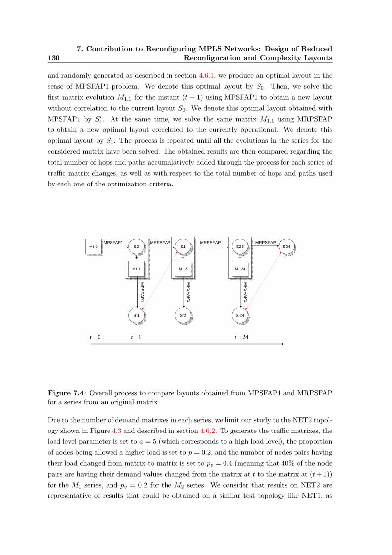
1307. Contribution to Reconfiguring MPLS Networks: Design of Reduced
Reconfiguration and Complexity Layouts
and randomly generated as described in section 4.6.1, we produce an optimal layout in thesense of MPSFAP1 problem. We denote this optimal layout by S0. Then, we solve thefirst matrix evolution M1.1 for the instant (t + 1) using MPSFAP1 to obtain a new layoutwithout correlation to the current layout S0. We denote this optimal layout obtained withMPSFAP1 by S′1. At the same time, we solve the same matrix M1.1 using MRPSFAPto obtain a new optimal layout correlated to the currently operational. We denote thisoptimal layout by S1. The process is repeated until all the evolutions in the series for theconsidered matrix have been solved. The obtained results are then compared regarding thetotal number of hops and paths accumulatively added through the process for each series oftraffic matrix changes, as well as with respect to the total number of hops and paths usedby each one of the optimization criteria.
++
M1.0M1.0 S0S0MPSFAP1
M1.1M1.1
MRPSFAP
S’1S’1
MP
SFA
P1
++
S1S1
M1.2M1.2
S’2S’2
MP
SFA
P1
++
S23S23
M1.24M1.24
S’24S’24
MP
SFA
P1
S24S24MRPSFAP MRPSFAP
0=t 1=t 24=t
Figure 7.4: Overall process to compare layouts obtained from MPSFAP1 and MRPSFAPfor a series from an original matrix
Due to the number of demand matrixes in each series, we limit our study to the NET2 topol-ogy shown in Figure 4.3 and described in section 4.6.2. To generate the traffic matrixes, theload level parameter is set to a = 5 (which corresponds to a high load level), the proportionof nodes being allowed a higher load is set to p = 0.2, and the number of nodes pairs havingtheir load changed from matrix to matrix is set to pv = 0.4 (meaning that 40% of the nodepairs are having their demand values changed from the matrix at t to the matrix at (t+1))for the M1 series, and pv = 0.2 for the M2 series. We consider that results on NET2 arerepresentative of results that could be obtained on a similar test topology like NET1, as

7.6. Preliminary Results on MRPSFAP and Model Validation 131
it shows a higher connectivity (density of 2.5) and consequently a higher number of pathsthat can be changed. The importance of the complexity and reconfiguration objectives areequally weighted (ϕ = ν = 1). The end-to-end path delay constraints are in all cases keptas in Chapter 4. Next, results obtained for two traffic matrixes and their correspondingevolutions are shown.
10
12
14
16
0 1 2 3 4 5 6 7 8 9 10 11 12 13 14 15 16 17 18 19 20 21 22 23
Matrixes
Path
s
Paths - MPSFAP1Paths - MRPSFAP
(a) Paths, a = 5, p = 0.2, pv = 0.4
0
2
4
6
8
10
12
14
16
18
1 2 3 4 5 6 7 8 9 10 11 12 13 14 15 16 17 18 19 20 21 22 23 24
Matrixes
Path
s
Paths - MPSFAP1 - Accumulated AdditionsPaths - MRPSFAP - Accumulated Additions
(b) Accumulated path additions, a = 5, p = 0.2, pv =0.4
Figure 7.5: Used paths and accumulated path additions for MPSFAP1 and MRPSFAP onNET2 for demand matrix series M1
10
12
14
16
18
20
0 1 2 3 4 5 6 7 8 9 10 11 12 13 14 15 16 17 18 19 20 21 22 23Matrixes
Hop
s
Hops - MPSFAP1Hops - MRPSFAP
(a) Hops, a = 5, p = 0.2, pv = 0.4
0
5
10
15
20
25
30
35
1 2 3 4 5 6 7 8 9 10 11 12 13 14 15 16 17 18 19 20 21 22 23 24Matrixes
Hop
s
Hops - MPSFAP1 - Accumulated AdditionsHops - MRPSFAP - Accumulated Additions
(b) Accumulated hops additions, a = 5, p = 0.2, pv =0.4
Figure 7.6: Used hops and accumulated hop additions for MPSFAP1 and MRPSFAP onNET2 for demand matrix series M1
In Figures 7.5(b) and 7.6(b), we observe that the number of paths and hops accumulativelyadded through the optimization of the reconfiguration complexity operated by MRPSFAPfor the 24 traffic matrixes in the M1 series is significatively lower than the number of addi-

1327. Contribution to Reconfiguring MPLS Networks: Design of Reduced
Reconfiguration and Complexity Layouts
tions operated by independently optimizing only the layout complexity through MPSFAP1.
Paths Added and Deleted - MPSFAP
0
0,5
1
1,5
2
2,5
3
3,5
1 2 3 4 5 6 7 8 9 10 11 12 13 14 15 16 17 18 19 20 21 22 23 24Matrix
Path
s
Paths Added MPSFAPPaths Deleted MPSFAP
Addings Average
Deletions Average
(a) MPSFAP1, a = 5, p = 0.2, pv = 0.4
Paths Added and Deleted - MRPSFAP
0
0,5
1
1,5
2
2,5
3
3,5
1 2 3 4 5 6 7 8 9 10 11 12 13 14 15 16 17 18 19 20 21 22 23 24Matrix
Path
s
Paths Added MRPSFAPPaths Deleted MRPSFAP
Addings Average
Deletions Average
(b) MRPSFAP, a = 5, p = 0.2, pv = 0.4
Figure 7.7: Path additions and deletions for MPSPAF1 and MRPSFAP for demand matrixseries M1
Hops Added and Deleted - MPSFAP
0
1
2
3
4
5
6
1 2 3 4 5 6 7 8 9 10 11 12 13 14 15 16 17 18 19 20 21 22 23 24Matrix
Hop
s
Hops Added MPSFAPHops Deleted MPSFAP
Addings Average
Deletions Average
(a) MPSFAP1, a = 5, p = 0.2, pv = 0.4
Hops Added and Deleted - MRPSFAP
0
1
2
3
4
5
6
1 2 3 4 5 6 7 8 9 10 11 12 13 14 15 16 17 18 19 20 21 22 23 24Matrix
Hop
s
Hops Added MRPSFAPHops Deleted MRPSFAP
Addings Average
Deletions Average
(b) MRPSFAP, a = 5, p = 0.2, pv = 0.4
Figure 7.8: Hop additions and deletions for MPSPAF1 and MRPSFAP for demand matrixseries M1
By examining Figures 7.5(a) and 7.6(a) we see that layouts obtained by both MPSFAP1and MRPSFAP use almost the same quantity of hops and paths through the whole series.The last shows that MRPSFAP optimizes the layout complexity, as well as the reconfigura-tion complexity during transitions, which is the objective we aim at for the design of MPLSlayouts under dynamic traffic conditions. Also, as the traffic conditions vary significativelyfrom one matrix to the next in M1 (since pv = 0.4 in this series), the number of hops andpaths also changes to adapt to those variations. However, on some cases MRPSFAP ap-pears to use more hops and paths than MPSFAP1, but we see that those cases correspond

7.6. Preliminary Results on MRPSFAP and Model Validation 133
to the transitions when additions have to be done and in that case, MRPSFAP is choosingto use one more path (or a longer one in hops) to keep the number of additions low. It isimportant to note that from the results obtained, we verify that the fact of including onlythe weighted path additions in the cost function helps the network to adapt to a decreasein the load level by allowing it to reduce the number of paths in the optimal layout. If pathdeletions were penalized as the additions, MRPSFAP would rather choose a higher numberof paths than required for a given traffic load, leading to a non-efficient resource usage.
10
12
14
16
0 1 2 3 4 5 6 7 8 9 10 11 12 13 14 15 16 17 18 19 20 21 22 23
Matrixes
Path
s
Paths - MPSFAP1Paths - MRPSFAP
(a) Paths, a = 5, p = 0.2, pv = 0.2
0
5
10
15
20
25
1 2 3 4 5 6 7 8 9 10 11 12 13 14 15 16 17 18 19 20 21 22 23 24
Matrixes
Path
s
Paths - MPSFAP1 - Accumulated AdditionsPaths - MRPSFAP - Accumulated Additions
(b) Accumulated path additions, a = 5, p = 0.2, pv =0.2
Figure 7.9: Used paths and accumulated path additions for MPSFAP1 and MRPSFAP onNET2 for demand matrix series M2
10
12
14
16
18
0 1 2 3 4 5 6 7 8 9 10 11 12 13 14 15 16 17 18 19 20 21 22 23Matrixes
Hop
s
Hops - MPSFAP1Hops - MRPSFAP
(a) Hops, a = 5, p = 0.2, pv = 0.2
0
5
10
15
20
25
30
35
40
45
1 2 3 4 5 6 7 8 9 10 11 12 13 14 15 16 17 18 19 20 21 22 23 24Matrixes
Hop
s
Hops - MPSFAP1 - Accumulated AdditionsHops - MRPSFAP - Accumulated Additions
(b) Accumulated hops additions, a = 5, p = 0.2, pv =0.2
Figure 7.10: Used hops and accumulated hop additions for MPSFAP1 and MRPSFAP onNET2 for demand matrix series M2
Figures 7.7(a), 7.7(b), 7.8(a) and 7.8(b) show the detailed path and hops additions and

1347. Contribution to Reconfiguring MPLS Networks: Design of Reduced
Reconfiguration and Complexity Layouts
deletions operated by both MPSFAP1 and MRPSFAP for the 24 matrixes in the M1 se-ries. We see that the addition and deletion activity is always lower for MRPSFAP thanfor MPSFAP1 for both paths and hops. In conclusion, MRPSFAP requires in general lesschanges (i.e. additions) than MPSFAP1 to realize a series of traffic adaptations, and whenthose changes have to be done, they are in general shorter (in hops) than those operatedby MPSFAP1.
Paths Added and Deleted - MPSFAP
0
0,5
1
1,5
2
2,5
3
3,5
4
4,5
1 2 3 4 5 6 7 8 9 10 11 12 13 14 15 16 17 18 19 20 21 22 23 24Matrix
Path
s
Paths Added MPSFAPPaths Deleted MPSFAP
Addings Average
Deletions Average
(a) MPSFAP1, a = 5, p = 0.2, pv = 0.2
Paths Added and Deleted - MRPSFAP
0
0,5
1
1,5
2
2,5
3
3,5
4
4,5
1 2 3 4 5 6 7 8 9 10 11 12 13 14 15 16 17 18 19 20 21 22 23 24Matrix
Path
s
Paths Added MRPSFAPPaths Deleted MRPSFAP
Addings AverageDeletions Average
(b) MRPSFAP, a = 5, p = 0.2, pv = 0.2
Figure 7.11: Path additions and deletions for MPSPAF1 and MRPSFAP for demandmatrix series M2
Hops Added and Deleted - MPSFAP
0
1
2
3
4
5
6
7
8
1 2 3 4 5 6 7 8 9 10 11 12 13 14 15 16 17 18 19 20 21 22 23 24Matrix
Hop
s
Hops Added MPSFAPHops Deleted MPSFAP
Addings Average
Deletions Average
(a) MPSFAP1, a = 5, p = 0.2, pv = 0.2
Hops Added and Deleted - MRPSFAP
0
1
2
3
4
5
6
7
8
1 2 3 4 5 6 7 8 9 10 11 12 13 14 15 16 17 18 19 20 21 22 23 24Matrix
Hop
s
Hops Added MRPSFAPHops Deleted MRPSFAP
Addings Average
Deletions Average
(b) MRPSFAP, a = 5, p = 0.2, pv = 0.2
Figure 7.12: Hop additions and deletions for MPSPAF1 and MRPSFAP for demand matrixseries M2
When the variations in the traffic matrix are less significative (pv = 0.2), we see from Figures7.9(a) and 7.10(a)1 that the number of paths and hops stays almost unchanged for layouts
1No value in the chart means that the particular traffic matrix was infeasible. Accumulated values are not

7.7. Extensions for Multiple Classes of Service 135
obtained from both optimization objectives, except in early matrixes, when MRPSFAPused solutions with longer paths in order to avoid path and hops additions. However, fromFigures 7.9(b) and 7.10(b) it can be seen that MPSFAP1 accumulates additions through theset of matrix changes, even when changes in the layout do not lead to better values in theobjective function (i.e. optimality in the sense of MPSFAP1 problem). Again, from Figures7.11(a), 7.11(b), 7.12(a) and 7.12(b) we observe that the activity of path and hops additionsand deletions is higher for MPSFAP1. Here the difference is accentuated by the fact thatan important number of those changes were not needed for the given traffic changes, andas such MRPSFAP guarantees that changes are done when they become unavoidable.
7.7. Extensions for Multiple Classes of Service
MRPSFAPQ 1Minimum Reconfiguration, Path Set and Flow Allocation Problem for Multiple Classes ofService
Given:
A,C,Dl,(t+1),H(t),Θ,∆,W
minimize :
ϕ
L∑l=1
tW(l) ·Hl,(t+1) + ν
L∑l=1
tW(l) · Sl,(t+1) (7.15)
subject to:
X(t+1) = A ·B(t+1) · 1lL ≤ C (7.16)
R ·B(t+1) = D(t+1) (7.17)
hkq,l(t+1)
M∑i=1
λakq,iCi − xi(t+1)
≤ θq,l l = 1, . . . , L; k = 1, . . . ,Kq; q = 1, . . . , Q (7.18)
bkq,l(t+1) ≤ hkq,l(t+1)δq,l l = 1, . . . , L; k = 1, . . . ,Kq; q = 1, . . . , Q (7.19)
(hkq,l(t+1) − hkq,l(t))h
kq,l(t+1) ≤ s
kq,l(t+1) l = 1, . . . , L; k = 1, . . . ,Kq; q = 1, . . . , Q (7.20)
hkq,l(t+1) ∈ {0, 1} l = 1, . . . , L; k = 1, . . . ,Kq; q = 1, . . . , Q (7.21)
skq,l(t+1) ∈ {0, 1} l = 1, . . . , L; k = 1, . . . ,Kq; q = 1, . . . , Q (7.22)
bkq,l(t+1) ≥ 0 l = 1, . . . , L; k = 1, . . . ,Kq; q = 1, . . . , Q (7.23)
Recalling the model extensions for multiple classes of service in section 4.7, the problemof reconfiguration and layout complexity can be extended to a Minimum Reconfiguration,
affected.

1367. Contribution to Reconfiguring MPLS Networks: Design of Reduced
Reconfiguration and Complexity Layouts
Path Set and Flow Allocation Problem for Multiple Classes of Service (MRPSFAPQ). Thedemand matrix D defined in (4.27) considering multiple commodities for each node pairis now individualized in time: D(t) is the demand matrix for instant t, and D(t+1) is thedemand matrix for calculating the new layout (instant (t+1)). Similarly, B(t) as defined in(4.28) and H(t), are the current path flow matrix and used path matrix, while B(t+1) andH(t+1) are the corresponding matrixes for the new layout at (t+ 1). The classes of serviceare indexed l = 1, . . . , L.
7.8. Conclusions
In this Chapter, the traffic dynamics have been considered. In this context, we find that forlarge networks and even when the MPLS layouts for successive demand matrixes are cal-culated according to the objectives defined for the MPSFAP problems, the reconfigurationcomplexity can be also very large, increasing the operational costs due to reconfigurationof the network. The reconfiguration costs can be even higher than the cost of operatingthe network in a sub-optimal state. The major contribution in this Chapter consist in thedefinition of a cost function for the optimization of the new layout, which has takes intoaccount the currently used layout, in order to minimize complexity of the new layout as wellas minimizing the reconfiguration complexity. The formulated problem is then referred asMRPSFAP (Minimum Reconfiguration and Path Set Flow Allocation Problem). The prob-lem is formulated mathematically, as in the MPSFAP problems in Chapter 4, as a MINLPproblem. Constraints are included so as to guarantee some QoS parameters as throughputand end-to-end path delay. Here again, the complexity of the problem formulated limitsthe tractable size of the problems by use of a deterministic solver.
In order to validate the model we resort to a deterministic solver, obtaining results forsmall network topologies. Results are obtained for two matrixes representing a mild toheavy load condition, from which a series of 24 traffic matrixes are generated. Results forthe MRPSFAP problem are compared against results obtained by solving as if each trafficmatrix were solved independently using the MPSFAP objective alone. Results show that wesignificatively reduce the number of hops and paths having to be changed from one layoutto the next one as the traffic matrix evolves in time. In order to deal with the problem sizelimitation when using deterministic solvers, an heuristic based on a further adaptation ofthe MFD presented in Chapter 5 is developed in the next Chapter.

8. Contribution to the Development of Heuristics for Solving the
Minimum Reconfiguration and Path Set Flow Allocation
Problem (MPRSFAP)
8.1. Selecting Efficient Heuristics
As the MPSFAP problems, the MRPSFAP problem is also NP-complete. In Chapter 7 theMRPSFAP problem was evaluated for small networks, which allowed us to to acquire someinsight into the behavior of the objective function with respect to the MPSFAP objectives,and somewhat determine the interest of such optimization objectives for the design of MPLSlayouts. However, heuristics are needed to solve large instances of the MRPSFAP problemdue to the problem size limitations of the deterministic methods used in available solvers.In Chapter 5, meta-heuristics and ad-hoc heuristics for solving the dimensioning problems(MPSFAP) formulated in Chapter 4 were developed and evaluated. Algorithms implement-ing meta-heuristics based on Tabu Search methods (TS), as well as ad-hoc heuristics basedon the Modified Flow Deviation method (MFD) were developed and tested both on smalland large topologies. In Chapter 6, the implemented algorithms were evaluated for largenetworks under the same conditions (i.e. on the same hardware and operating environment),leading to the confirmation of the interest in including reconfiguration objectives togetherwith dimensioning objectives for the design of MPLS layouts.
Analyzing the quality of the results obtained for the MPLS layout optimization of MPSFAPobjectives on large networks, together with the corresponding computational effort theyrequire, we conclude that the Tabu Search algorithm implemented is largely outperformed bythe Modified Flow Deviation algorithm. Both, the quality of the results in terms of the valueof the objective function, but mainly the computational performance of the MFD comparedto the TS algorithms, encourage us to further develop ad-hoc heuristics in order to find asuitable and efficient algorithm to solve the MRPSFAP problem. In particular, the MFDalgorithm implemented in section 5.5 in Chapter 5 already presents characteristics that makeit naturally well adapted to efficiently solve the MRPSFAP problem with few modifications.In what follows, we present our contribution to the development of heuristics for solving theMRPSFAP problem, the Modified Flow Deviation Algorithm for Reconfiguration (MFD-R),describing the modifications introduced to the MFD described.
137

1388. Contribution to the Development of Heuristics for Solving the Minimum
Reconfiguration and Path Set Flow Allocation Problem (MPRSFAP)
8.2. Adapting the Modified Flow Deviation Algorithm (MFD) for Solving the
MRPSFAP Problem
Recalling from section 5.5, the basic idea behind the MFD algorithm is to start from ashortest path layout in terms of number of hops, which can be feasible or infeasible withrespect to the constraints (4.13),(4.14) and(4.15) defined in Chapter 4, and then shift flowon one node pair at a time in the direction of reducing the value of the objective function,which is defined as a function of the overload on the link (besides the weighted sum of theused paths). As such, decreasing the value of the objective function ensures that we shiftflow also in the direction of converting the current solution into a feasible solution. Theprocedure of shifting flow on a node pair basis starting from a shortest path layout withsingle multiplicity (i.e. only one path connecting each node pair), ensures that the minimumquantity of paths (and shortest in quantity of hops) are added in the process, so when thelayout obtained after a given iteration is feasible, it will likely be also the optimal in terms ofMPSFAP1 objective. This has been shown when evaluating results for the MFD algorithmin section 5.5.6.
The algorithm finishes if no candidate is found to make a flow shift in the direction of de-creasing the overload in the network or shift direction. If this happens and the constraintsare still not met, we conclude that the problem is infeasible. However, we are not sure thatthe problem is infeasible if we have not tested all possible candidates in the set of paths.To improve the algorithm we introduce a modified version in Algorithm 5.6 to make appearall possible candidates before declaring the problem infeasible.
The MFD algorithm can be easily adapted to solve the MRPSFAP problem taking advantageof the particular characteristics of the above described procedure. The way we initialize thealgorithm and the flow shift direction are chosen in a node pair basis guarantee that thesolution found will be near-optimal in the sense of MPSFAP1 objective. However, theshift direction is searched among all the possible paths, what doesn’t take into account thecurrently used paths. Indeed, a path that is not being used in the current layout can appearas a candidate to have flow shifted in, what would produce a path addition. We need tomodify the way we chose the shift direction in order to explore first the paths that are beingcurrently used and if no shift direction can be found, then all possible paths are explored.This will produce layouts with a low number of path additions, weighted by their lengthsin hop-counts. However, it must be noted that no solution obtained through the MFDalgorithm can be guaranteed to be globally optimal, since the order in which the flow shiftsare realized affects the progression of the algorithm. We can control the order in which flowshifts are made by means of the choice index defined in Algorithm 5.11.

8.3. A Modified Flow Deviation Algorithm for Reconfiguration (MFD-R) 139
8.3. A Modified Flow Deviation Algorithm for Reconfiguration (MFD-R)
Formally, given the current operational layout H(t) and the new demand matrix D(t+1)
(along with A, Θ, W and C), Algorithm 5.6 is modified to find the new set of used pathsH(t+1) and path flow vector B(t+1).
Algorithm 8.1 includes the modifications introduced to the MFD algorithm, mainly regard-ing the way the set of paths in the arc-path incidence matrix A is explored. In the versionof the algorithm to solve the MPSFAP1 problem, the whole matrix is explored on everyiteration, since no reconfiguration objective is considered. When the reconfiguration objec-tive is included, the way in which the set of paths is explored to find a shift direction whichwould produce a decrease in the value of the objective function becomes a key factor. If allpaths in A are explored at each iteration as in the MFD algorithm, then paths that are notin H(t) could result included inH(t+1) (i.e. paths that are not used in the current layout)when searching for a shift direction. The set of paths to explore in a particular iteration ofthe algorithm is increased as no shift direction is found in the current set, until the wholematrix A has been searched or a shift direction found.
8.3.1. Initialization: The Initial Layout
The first modification consists in the way the initial layout is generated. One shortest pathper node pair is found within the set of currently used paths H(t) instead of within thewhole matrix A as in MFD. This guarantees that the initial proposed solution exclusivelyuses paths in the set of paths that were already used in the current solution. Algorithm 8.2calculates the single shortest path for every node pair within the set given as argument. Inthe initialization phase it is called with H(t), so the returned set of shortest paths P containspaths only in the set H(t). Later in the MFD-R algorithm, the procedure for calculatingthe set of single shortest paths is called with different set of paths to progressively includelarger set of candidates if no shift direction could be found in sets containing already usedpaths.
Require: F,V {V is the set of paths within which the shortest paths must be determined}Ensure: P
P ={akq : mink
{F kq}∧ akq ∈ V
}Return P
Algorithm 8.2: Pseudo Code for Calculating the Set of Shortest Paths Within a Path Set

1408. Contribution to the Development of Heuristics for Solving the Minimum
Reconfiguration and Path Set Flow Allocation Problem (MPRSFAP)
Require: A,Θ,W,D(t+1),C,H(t) as defined in Chapter 7Ensure: B(t+1),H(t+1) or INFEASIBLE
B(t+1) ← 0H(t+1) ← ∅ {set of currently used paths}F←W∆B(t+1) ← 0P← ∅ {set of current shortest paths}P← find shortest paths(F,H(t))for all (akq ∈ P) dobkq,(t+1) ← dq,(t+1) {assign all the demands to the shortest paths}
end forH(t+1) ← PX(t+1) ← A ·B(t+1)
F← update path weights(X(t+1))P← find shortest paths(F,H(t) ∪H(t+1))∆B(t+1) ← find shift direction(B(t+1),P,H(t+1),F)if (∆B(t+1) = 0) and (constraints are not met) then
∆B(t+1) ← examine thresholds(F,H(t) ∪H(t+1),B(t+1),H(t+1))if (∆B(t+1) = 0) then
P← find shortest paths(F,A)while (∆B(t+1) = 0) do
∆B(t+1) ← examine thresholds(F,A,B(t+1),H(t+1))end while
end ifend ifwhile (∆B(t+1) 6= 0) doφ← find shift factor(∆B(t+1),X(t+1))B(t+1) ← B(t+1) + φ∆B(t+1)
X(t+1) ← A ·B(t+1)
H(t+1) ← ∪k=1,...,Kq ;q=1,...,Q
{akq : bkq,(t+1) > 0
}F← update path weights(X(t+1))P← find shortest paths(F,H(t) ∪H(t+1))∆B(t+1) ← find shift direction(B(t+1),P,H(t+1),F)if (∆B(t+1) = 0) and (constraints are not met) then
∆B(t+1) ← examine thresholds(F,H(t) ∪H(t+1),B(t+1),H(t+1))if (∆B(t+1) = 0) then
P← find shortest paths(F,A)while (∆B(t+1) = 0) do
∆B(t+1) ← examine thresholds(F,A,B(t+1),H(t+1))end while
end ifend if
end whileif constraints are met then
Return B(t+1),H(t+1)
elseReturn INFEASIBLE
end ifAlgorithm 8.1: Pseudo-code for the Modified Flow Deviation Method Applied to theMRPSFAP Problem

8.3. A Modified Flow Deviation Algorithm for Reconfiguration (MFD-R) 141
8.3.2. Search for a Shift Direction: Progressive Exploration
Once the initial layout established, it can result feasible or unfeasible. If it is feasible (i.e.constraints are met) the algorithm has found a feasible solution with the minimum numberof hops using paths that were already used in the previous solution. If the initial layoutis infeasible, then the algorithm starts iterating until a feasible layout is found or no shiftdirection could be found (in which case we declare the problem infeasible). The mainiteration in Algorithm 8.1 ensures a way of finding a shift direction that explores all thepossible candidates by increasing the size of the set in which paths are searched for as noshift direction could be found in smaller sets. There are two possible sets to consider:
• The set of used paths in the current layout along with the set of currently used pathsin the iteration: H(t) ∪H(t+1).
• The whole arc-path incidence matrix A.
As long as a shift direction can be found in the set H(t) ∪H(t+1), we are sure that pathsbeing included in H(t+1) were already used in the layout at t or were already introduced inthe current layout being calculated at (t + 1) because the shift direction had to be foundlooking in A in a previous iteration. At each iteration, the search is narrowed again, asthe path weights are updated making possibly appear new candidates in the smaller set.Algorithm 8.3 examines all possible candidates within the set given as argument accordingto the improvement introduced in Algorithm 5.6.
Require: F,V,B(t+1),H(t+1) {V is the set of paths to explore for a shift direction}Ensure: ∆B(t+1) > 0 if a possible shift direction exists, and 0 otherwise.
∆B(t+1) ← 0threshold← 1Fb ← Fwhile (∆B(t+1) = 0) and (threshold < network diameter) do
Fb ← increase threshold level(Fb, threshold)P← find shortest paths(F,V)∆B(t+1) ← find shift direction(B(t+1),P,H(t+1),Fb)threshold← threshold+ 1
end whileReturn ∆B(t+1)
Algorithm 8.3: Pseudo Code for Examining All Possible Candidates for a Shift DirectionWithin a Given Set of Paths
The procedures to calculate the shift direction, the shift factor and the choice index, definedin Algorithms 5.9, 5.10 and 5.11 stay the same as defined in Chapter 5, except that theyare called with the instances at (t+ 1) of the path flow vector B(t+1) and used path matrixH(t+1). All the other algorithms defined in section 5.5 do not need to be modified either,and are used as before.

1428. Contribution to the Development of Heuristics for Solving the Minimum
Reconfiguration and Path Set Flow Allocation Problem (MPRSFAP)
8.4. Evaluation of the MFD-R Algorithm for MRPSFAP
In this section we first evaluate the Modified Flow Deviation for Reconfiguration (MFD-R)heuristic by comparing the results obtained from the MINLP deterministic solver for a smallnetwork topology (NET2) in Chapter 7, to the results obtained from the MFD-R algorithmfor the set of matrixes M1. Second, we obtain results for large network topologies such asVTHD and NSF presented in Chapter 6, using the MFD-R algorithm for two set of matrixesMV THD
1 and MNSF1 .
8.4.1. Evaluation of the MFD-R Algorithm on Small Networks
In order to evaluate the MFD-R algorithm, we compare the results obtained for NET2network topology of previous chapters by using both, the MFD-R and the deterministicsolver (MINLP). As before, we use a small topology to evaluate the algorithm due to theproblem size limitations of the deterministic solver. The same set of matrixes M1 of Chapter7 is used to compare results for MFD-R and MINLP solver, and all runs for MFD-R aremade under the same conditions on the same machine. Figure 8.1(a) shows the total numberof hops required by MRPSFAP by using both MFD-R and the MINLP solver.
10
12
14
16
18
20
0 1 2 3 4 5 6 7 8 9 10 11 12 13 14 15 16 17 18 19 20 21 22 23Matrix
Hop
s
Hops - MRPSFAP(NEOS)Hops - MRPSFAP(MFD)
(a) Active Hops
0
5
10
15
20
25
30
35
1 2 3 4 5 6 7 8 9 10 11 12 13 14 15 16 17 18 19 20 21 22 23 24Matrix
Hop
s
Hops - MPSFAP(NEOS) - Accumulated Additions
Hops - MRPSFAP(NEOS) - Accumulated Additions
Hops - MPSFAP(MFD) - Acummulated Additions
Hops - MRPSFAP(MFD) - Acummulated Additions
(b) Accumulated Hop Additions
Figure 8.1: Used hops and accumulated hop additions for MPSFAP1 and MRPSFAP onNET2 for demand matrix series M1 using MINLP Solver (NEOS) and MFD-R Heuristic
From the figure, we see that the number of hops required when solving the MRPSFAPproblem with MFD is greater than the number of hops required when solving the sameinstance with the deterministic solver. From Figure 8.2(a) we observe the same trend forthe number of paths. Not surprisingly, this conclusion for the MFD-R algorithm (observedalso for the MFD algorithm applied to the MPSFAP problems) was somewhat expected.In fact, both the MFD and MFD-R algorithms are heuristics to find approximate solutionsto a complex problems, tackling the size limitations imposed by the deterministic solvers.
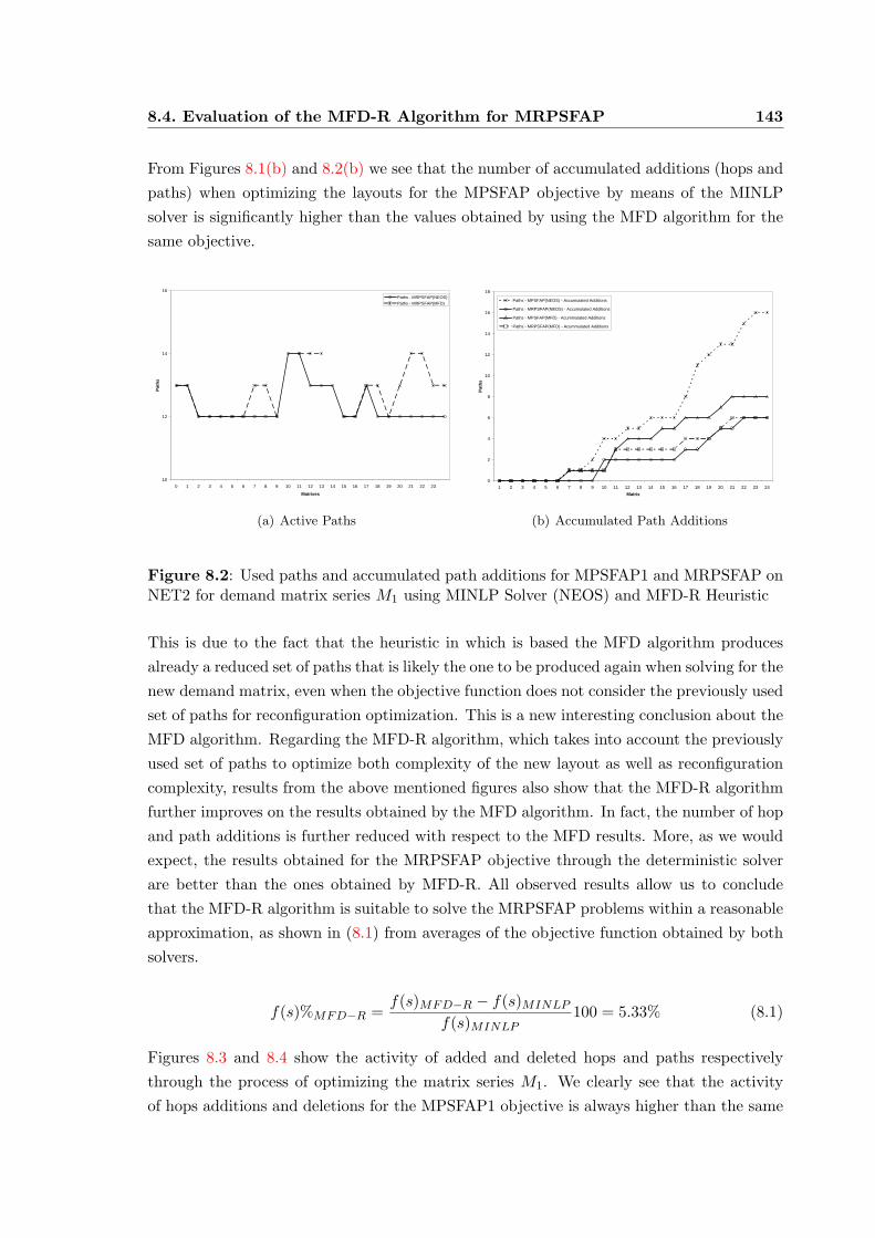
8.4. Evaluation of the MFD-R Algorithm for MRPSFAP 143
From Figures 8.1(b) and 8.2(b) we see that the number of accumulated additions (hops andpaths) when optimizing the layouts for the MPSFAP objective by means of the MINLPsolver is significantly higher than the values obtained by using the MFD algorithm for thesame objective.
10
12
14
16
0 1 2 3 4 5 6 7 8 9 10 11 12 13 14 15 16 17 18 19 20 21 22 23
Matrixes
Path
s
Paths - MRPSFAP(NEOS)Paths - MRPSFAP(MFD)
(a) Active Paths
0
2
4
6
8
10
12
14
16
18
1 2 3 4 5 6 7 8 9 10 11 12 13 14 15 16 17 18 19 20 21 22 23 24Matrix
Path
s
Paths - MPSFAP(NEOS) - Accumulated Additions
Paths - MRPSFAP(NEOS) - Accumulated Additions
Paths - MPSFAP(MFD) - Acummulated Additions
Paths - MRPSFAP(MFD) - Acummulated Additions
(b) Accumulated Path Additions
Figure 8.2: Used paths and accumulated path additions for MPSFAP1 and MRPSFAP onNET2 for demand matrix series M1 using MINLP Solver (NEOS) and MFD-R Heuristic
This is due to the fact that the heuristic in which is based the MFD algorithm producesalready a reduced set of paths that is likely the one to be produced again when solving for thenew demand matrix, even when the objective function does not consider the previously usedset of paths for reconfiguration optimization. This is a new interesting conclusion about theMFD algorithm. Regarding the MFD-R algorithm, which takes into account the previouslyused set of paths to optimize both complexity of the new layout as well as reconfigurationcomplexity, results from the above mentioned figures also show that the MFD-R algorithmfurther improves on the results obtained by the MFD algorithm. In fact, the number of hopand path additions is further reduced with respect to the MFD results. More, as we wouldexpect, the results obtained for the MRPSFAP objective through the deterministic solverare better than the ones obtained by MFD-R. All observed results allow us to concludethat the MFD-R algorithm is suitable to solve the MRPSFAP problems within a reasonableapproximation, as shown in (8.1) from averages of the objective function obtained by bothsolvers.
f(s)%MFD−R =f(s)MFD−R − f(s)MINLP
f(s)MINLP100 = 5.33% (8.1)
Figures 8.3 and 8.4 show the activity of added and deleted hops and paths respectivelythrough the process of optimizing the matrix series M1. We clearly see that the activityof hops additions and deletions for the MPSFAP1 objective is always higher than the same

1448. Contribution to the Development of Heuristics for Solving the Minimum
Reconfiguration and Path Set Flow Allocation Problem (MPRSFAP)
activity for the MRPSFAP objective. Regarding the performance of the MFD-R algorithmas compared to the deterministic solver, we see that the average figures for additions anddeletions for the MFD-R algorithm are only slightly higher than the ones observed for theMINLP solver.
Hops Added and Deleted - MPSFAP (NEOS vs. MFD)
0
1
2
3
4
5
6
1 2 3 4 5 6 7 8 9 10 11 12 13 14 15 16 17 18 19 20 21 22 23 24Matrix
Hop
s
Hops Added MPSFAP(NEOS)Hops Deleted MPSFAP(NEOS)Hops Addes MPSFAP(MFD)Hops Deleted MPSFAP(MFD)
Addings and DeletionsAverage (NEOS) = 1.16
Addings and DeletionsAverage (MFD) = 0.65
(a) MPSFAP1
Hops Added and Deleted - MRPSFAP (NEOS vs. MFD)
0
1
2
3
4
5
6
1 2 3 4 5 6 7 8 9 10 11 12 13 14 15 16 17 18 19 20 21 22 23 24Matrix
Hop
s
Hops Added MRPSFAP(NEOS)Hops Deleted MRPSFAP(NEOS)Hops Added MRPSFAP(MFD)Hops Deleted MRPSFAP(MFD)
Addings and DeletionsAverage (NEOS) = 0.46
Addings and DeletionsAverage (MFD) = 0.50
(b) MRPSFAP
Figure 8.3: Hops added and deleted for MPSFAP1 and MRPSFAP on NET2 for demandmatrix series M1 using MINLP Solver (NEOS) and MFD-R Heuristic
Paths Added and Deleted - MPSFAP (NEOS vs. MFD)
0
0,5
1
1,5
2
2,5
3
3,5
1 2 3 4 5 6 7 8 9 10 11 12 13 14 15 16 17 18 19 20 21 22 23 24Matrix
Path
s
Paths Added MPSFAP(NEOS)Paths Deleted MPSFAP(NEOS)Paths Added MPSFAP(MFD)Paths Deleted MPSFAP(MFD)
Addings and DeletionsAverage (NEOS) = 0.64
Addings and DeletionsAverage (MFD) = 0.35
(a) MPSFAP1
Paths Added and Deleted - MRPSFAP (NEOS vs. MFD)
0
0,5
1
1,5
2
2,5
3
3,5
1 2 3 4 5 6 7 8 9 10 11 12 13 14 15 16 17 18 19 20 21 22 23 24Matrix
Path
s
Paths Added MRPSFAP(NEOS)Paths Deleted MRPSFAP(NEOS)Paths Added MRPSFAP(MFD)Paths Deleted MPSFAP(MFD)
DeletionsAverage (NEOS) = 0.29
Addings and DeletionsAverage (MFD) = 0.27
AddingsAverage (NEOS) = 0.25
(b) MRPSFAP
Figure 8.4: Paths added and deleted for MPSFAP1 and MRPSFAP on NET2 for demandmatrix series M1 using MINLP Solver (NEOS) and MFD-R Heuristic
The average for additions and deletions (hops and paths) when using MFD as opposed toMFD-R confirm the observation already made for Figures 8.1 and 8.2 above. The averagesfor MFD are higher than the ones for MFD-R, but the difference with the MINLP solverwhen optimizing the MPSFAP objective alone are significantly higher, which shows thatMFD is an already suitable algorithm to reduce reconfiguration complexity, even when it

8.4. Evaluation of the MFD-R Algorithm for MRPSFAP 145
does not take into account the previously used set of paths.
In next section we compare results from the MFD-R algorithm with results from the MFDalgorithm for large networks. The conclusions we made in this section regarding the goodperformance of MFD for the reconfiguration objectives, even when the complexity alone wasbeing minimized, will be useful when studying the comparative performance of MFD-R.
8.4.2. Results on Reconfiguration from the MFD-R Algorithm on Large Networks
In this section we compare results obtained by using MFD and MFD-R algorithms to solvethe MPSFAP1 and MRPSFAP problems respectively on large networks. The large networktopologies used in this section are the VTHD and NSF networks presented in Chapter 6.A set of demand matrixes conforming matrix series obtained as described in section 7.6.1are presented to each topology. We denote by MV THD
1 the matrix series presented to theVTHD network, and MNSF
1 the matrix series presented to the NSF network.
130
132
134
136
138
140
142
144
0 1 2 3 4 5 6 7 8 9 10 11 12 13 14 15 16 17 18 19 20 21 22 23Matrix
Hop
s
Hops - MPSFAPHops - MRPSFAP
(a) Active Hops
0
5
10
15
20
25
30
1 2 3 4 5 6 7 8 9 10 11 12 13 14 15 16 17 18 19 20 21 22 23 24Matrix
Hop
s
Hops - MPSFAP - Accumulated Additions
Hops - MRPSFAP - Accumulated Additions
(b) Accumulated Hop Additions
Figure 8.5: Active hops and accumulated hop additions for MPSFAP1 and MRPSFAP onVTHD for demand matrix series MV THD
1 using MFD and MFD-R heuristics
Figures 8.5(a) and 8.9(a) show the total number of active hops for each of the matrixes inthe corresponding series for VTHD and NSF topologies, when solving each of the matrixesfor the MPSFAP1 objective and the MRPSFAP objective. Figures 8.6(a) and 8.10(a) showthe corresponding values for the total number of used paths. We can observe for VTHD thatexactly the same number of hops and paths is used when solving either for the objectiveMPSFAP1 or MRPSFAP. Looking at Figures 8.5(b) and 8.6(b) we can see that the numberof accumulated hop and path additions is higher when solving the matrix series for theobjective MPSFAP1 (algorithm MFD) than for the objectiveMRPSFAP (algorithm MFD-R), although the difference is not much significant. Looking however to the quantity of

1468. Contribution to the Development of Heuristics for Solving the Minimum
Reconfiguration and Path Set Flow Allocation Problem (MPRSFAP)
active hops and paths for NSF, we can see that the number of hops required by MRPSFAPis generally higher than the number of hops required by MPSFAP1, while the number ofpaths required by MRPSFAP is always lower than the number required by MPSFAP1.
69
69,5
70
70,5
71
71,5
72
72,5
0 1 2 3 4 5 6 7 8 9 10 11 12 13 14 15 16 17 18 19 20 21 22 23
Matrixes
Path
s
Paths - MPSFAPPaths - MRPSFAP
(a) Active Paths
0
2
4
6
8
10
12
1 2 3 4 5 6 7 8 9 10 11 12 13 14 15 16 17 18 19 20 21 22 23 24
Matrixes
Path
s
Paths - MPSFAP - Accumulated AdditionsPaths - MRPSFAP - Accumulated Additions
(b) Accumulated Path Additions
Figure 8.6: Active paths and accumulated path additions for MPSFAP1 and MRPSFAPon VTHD for demand matrix series MV THD
1 using MFD and MFD-R heuristics
Hops Added and Deleted - MPSFAP
0
1
2
3
4
5
6
7
8
9
1 2 3 4 5 6 7 8 9 10 11 12 13 14 15 16 17 18 19 20 21 22 23 24Matrix
Hop
s
Hops Added MPSFAP
Hops Deleted MPSFAP
Addings Average = 1.00
Deletions Average = 1.08
(a) MPSFAP1
Hops Added and Deleted - MRPSFAP
0
1
2
3
4
5
6
7
8
9
1 2 3 4 5 6 7 8 9 10 11 12 13 14 15 16 17 18 19 20 21 22 23 24Matrix
Hop
s
Hops Added MRPSFAP
Hops Deleted MRPSFAP
Addings Average = 0.54
Deletions Average = 0.71
(b) MRPSFAP
Figure 8.7: Hops added and deleted for MPSFAP1 and MRPSFAP on VTHD for demandmatrix series MV THD
1 using MINLP Solver (NEOS) and MFD-R heuristics
This is a somewhat expected result, since the MFD-R heuristic concentrate in finding afeasible solution within the set of already used paths first, and then it looks for new pathsonly when no shift direction could be produced within the previously used set. This produceslayouts with a set of paths likely to be a subset of the previously used set for the MRPSFAPobjective, paying the cost of longer paths in order to reduce path additions with respect tothe previous set, while the MPSFAP1 objective is free to chose the shortest paths at every

8.4. Evaluation of the MFD-R Algorithm for MRPSFAP 147
iteration without any reference to the past.
Paths Added and Deleted - MPSFAP
0
0,5
1
1,5
2
2,5
3
3,5
1 2 3 4 5 6 7 8 9 10 11 12 13 14 15 16 17 18 19 20 21 22 23 24Matrix
Path
s
Paths Added MPSFAP
Paths Deleted MPSFAP
Addings Average = 0.4
Deletions Average = 0.4
(a) MPSFAP1
Paths Added and Deleted - MRPSFAP
0
0,5
1
1,5
2
2,5
3
3,5
1 2 3 4 5 6 7 8 9 10 11 12 13 14 15 16 17 18 19 20 21 22 23 24Matrix
Path
s
Paths Added MRPSFAP
Paths Deleted MRPSFAP
Addings Average = 0.21
Deletions Average = 0.25
(b) MRPSFAP
Figure 8.8: Paths added and deleted for MPSFAP1 and MRPSFAP on VTHD for demandmatrix series MV THD
1 using MINLP Solver (NEOS) and MFD-R heuristics
375
380
385
390
395
400
405
410
415
0 1 2 3 4 5 6 7 8 9 10 11 12 13 14 15 16 17 18 19 20 21 22 23Matrix
Hop
s
Hops - MPSFAPHops - MRPSFAP
(a) Active Hops
0
50
100
150
200
250
300
1 2 3 4 5 6 7 8 9 10 11 12 13 14 15 16 17 18 19 20 21 22 23 24Matrix
Hop
s
Hops - MPSFAP - Accumulated Additions
Hops - MRPSFAP - Accumulated Additions
(b) Accumulated Hop Additions
Figure 8.9: Active hops and accumulated hop additions for MPSFAP1 and MRPSFAP onNSF for demand matrix series MNSF
1 using MFD and MFD-R heuristics
The number of accumulated hop and path additions for NSF in Figures 8.9(b) and 8.10(b)show a significant difference with the values observed for VTHD. The number of accumulatedhop and path additions for the MRSPFAP objective in the case of NSF results almostdoubled with respect to the same values for the MPSFAP1 objective. In fact, this can beexplained by the nature of the topologies considered. VTHD topology doesn’t offer as manypossible path combinations to connect a given node pair as NSF does, presenting criticallinks (e.g. links 12, 24, 9, 21, 11, 23, 10 and 22 in Figure 6.1) that are used by all pathsconnecting some node pairs (e.g. nodes 5, 4 and 9 in the same figure). The impact of
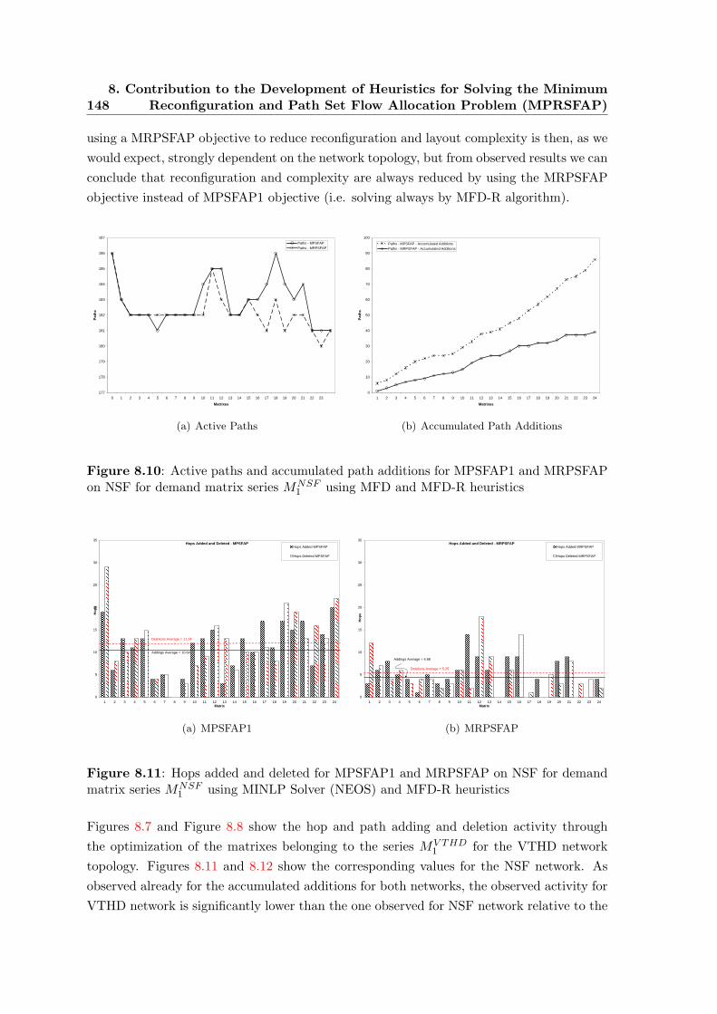
1488. Contribution to the Development of Heuristics for Solving the Minimum
Reconfiguration and Path Set Flow Allocation Problem (MPRSFAP)
using a MRPSFAP objective to reduce reconfiguration and layout complexity is then, as wewould expect, strongly dependent on the network topology, but from observed results we canconclude that reconfiguration and complexity are always reduced by using the MRPSFAPobjective instead of MPSFAP1 objective (i.e. solving always by MFD-R algorithm).
177
178
179
180
181
182
183
184
185
186
187
0 1 2 3 4 5 6 7 8 9 10 11 12 13 14 15 16 17 18 19 20 21 22 23
Matrixes
Path
s
Paths - MPSFAPPaths - MRPSFAP
(a) Active Paths
0
10
20
30
40
50
60
70
80
90
100
1 2 3 4 5 6 7 8 9 10 11 12 13 14 15 16 17 18 19 20 21 22 23 24
Matrixes
Path
s
Paths - MPSFAP - Accumulated AdditionsPaths - MRPSFAP - Accumulated Additions
(b) Accumulated Path Additions
Figure 8.10: Active paths and accumulated path additions for MPSFAP1 and MRPSFAPon NSF for demand matrix series MNSF
1 using MFD and MFD-R heuristics
Hops Added and Deleted - MPSFAP
0
5
10
15
20
25
30
35
1 2 3 4 5 6 7 8 9 10 11 12 13 14 15 16 17 18 19 20 21 22 23 24Matrix
Hop
s
Hops Added MPSFAP
Hops Deleted MPSFAP
Addings Average = 10.64
Deletions Average = 11.24
(a) MPSFAP1
Hops Added and Deleted - MRPSFAP
0
5
10
15
20
25
30
35
1 2 3 4 5 6 7 8 9 10 11 12 13 14 15 16 17 18 19 20 21 22 23 24Matrix
Hop
s
Hops Added MRPSFAP
Hops Deleted MRPSFAP
Addings Average = 4.88
Deletions Average = 5.25
(b) MRPSFAP
Figure 8.11: Hops added and deleted for MPSFAP1 and MRPSFAP on NSF for demandmatrix series MNSF
1 using MINLP Solver (NEOS) and MFD-R heuristics
Figures 8.7 and Figure 8.8 show the hop and path adding and deletion activity throughthe optimization of the matrixes belonging to the series MV THD
1 for the VTHD networktopology. Figures 8.11 and 8.12 show the corresponding values for the NSF network. Asobserved already for the accumulated additions for both networks, the observed activity forVTHD network is significantly lower than the one observed for NSF network relative to the

8.5. Conclusions 149
size of the corresponding networks.
Paths Added and Deleted - MPSFAP
0
1
2
3
4
5
6
7
8
9
10
1 2 3 4 5 6 7 8 9 10 11 12 13 14 15 16 17 18 19 20 21 22 23 24Matrix
Path
s
Paths Added MPSFAP
Paths Deleted MPSFAP
Addings Average = 3.44
Deletions Average = 3.64
(a) MPSFAP1
Paths Added and Deleted - MRPSFAP
0
1
2
3
4
5
6
7
8
9
10
1 2 3 4 5 6 7 8 9 10 11 12 13 14 15 16 17 18 19 20 21 22 23 24Matrix
Path
s
Paths Added MRPSFAP
Paths Deleted MRPSFAP
Addings Average = 1.63
Deletions Average = 1.79
(b) MRPSFAP
Figure 8.12: Paths added and deleted for MPSFAP1 and MRPSFAP on NSF for demandmatrix series MNSF
1 using MINLP Solver (NEOS) and MFD-R heuristics
It can also be observed that the additions and deletions are near symmetrical for VTHDnetwork, while they exhibit a greater asymmetry for the NSF network, the average ofdeletions being greater than the average of additions for both paths and hops, which isa wanted result. Finally, even when the average values for additions and deletions forVTHD network are relatively low, the ratio from values obtained for MPSFAP1 objectiveto the values obtained for MRPSFAP objective is almost the same than for NSF network(i.e. the averages for MRPSFAP are nearly half of the averages for MPSFAP1), whichdrives us to conclude that the MFD-R algorithm performs consistently well to optimize theMRPSFAP objective. Observed execution times for MFD-R are within the same order thanthe execution times observed for MFD under the same conditions.
8.5. Conclusions
The major contribution in the the present Chapter consists in the development of an heuris-tic method based on the MFD algorithm presented in Chapter 5. The MFD algorithm hasbeen shown to perform well both in the quality of the results obtained and in the executiontimes needed to calculate the layouts. Implementation of the algorithm has been completed,and further evaluation is presented in this chapter. Results obtained on small networks al-low us to conclude that the MFD-R algorithm performs within a reasonable range from theoptimal results obtained by using a deterministic solver (MINLP), and important conclu-sions were obtained about the behavior of the MFD and MFD-R algorithms. Finally, theMFD-R was evaluated for large networks, and results compared to the results obtained withthe MFD algorithm for the same traffic matrix series. The MFD-R algorithm has shown to

1508. Contribution to the Development of Heuristics for Solving the Minimum
Reconfiguration and Path Set Flow Allocation Problem (MPRSFAP)
perform within our expectations for optimizing the MRPSFAP objective of reconfigurationand layout complexity, and as a consequence, obtained results allows us to foresee practicalapplications of the MFD-R algorithm in an operational context. Also, comparison to resultsobtained with the MFD algorithm helped us to acquire further insight in the behavior ofboth objectives. As a final and important conclusion, the MFD-R algorithm can be usedin practical operational environments to calculate layouts with dramatic improvement un-der dynamic traffic situations both in the sense of layout complexity and reconfigurationcomplexity.

General Conclusions
This Chapter presents the general conclusions inferred from the studies described in thepresent document. We summarize the main contributions before giving the future researchdirections that stem from this work.
Contributions
This thesis concentrates on the traffic engineering mechanisms involved in the dynamic con-trol of the network behavior considering long-term timescales. We locate our work in thetechnological context of Next Generation IP Networks, where a unified transport based onIP protocol is envisaged. As such, and to allow the operator to provide QoS guaranteeswhile optimizing the network resources traffic engineering mechanisms have to be added toIP transport functionalities. Modelling the TE system as a closed loop control system, threemain control loops can be identified, each loop corresponding to a timescale. TE mecha-nisms inscribed within a particular timescale aim at helping to control the network behaviorin order to ensure that the main objectives of TE are met: to provide QoS guarantees whileensuring an efficient use of network resources. In the context of NG-IP networks, MPLSallows for the implementation of evolved TE mechanisms by providing the possibility ofestablishing source routed paths. In the long-term timescales, the TE tasks are oriented toplanning and dimensioning of the network according both to underwritten service contractsand to business objectives. From an operator’s point of view, the business objectives arerealized in a significative part through OPEX and CAPEX reduction. The contributions ofthis thesis are then mainly oriented in this sense, where we propose realistic objectives todimension the network according to the business objectives, while meeting the user orientedobjectives (i.e. QoS guarantees). Dimensioning the network in a dynamic context involvesthe reconfiguration aspects, as it is not enough to obtain an optimal layout for a new trafficmatrix if the transition from the old layout to the new layout is too complex that no oper-ational cost reduction is obtained in the process.
Dimensioning of MPLS Layouts. Once the network deployed, the cost of operation isrelated to the complexity of the network layout. In a connected oriented transport paradigm,as we assume to be the framework in the present work, the layout is represented by the setof paths connecting each node pair and the flows to be allocated to each path in order tomeet the demands. We consider that the complexity of this layout, and in consequence the
151
1528. Contribution to the Development of Heuristics for Solving the Minimum
Reconfiguration and Path Set Flow Allocation Problem (MPRSFAP)
cost of operation, is related to the total number of paths weighted by the quantity of hopseach path is using. The larger the network, the more important this cost becomes. TheQoS guarantees such as end-to-end path delay and throughput for a given node pair can beguaranteed through constraints, while the actual cost when calculating the optimal layoutfor a given traffic matrix is represented by the number of length-weighted paths the layoutrequires to route a given demand. In this sense, the MPSFAP problems are formulatedto optimize the layouts with respect to the quantity of total hops needed to route suchdemand. To our knowledge, no such optimization objectives have been considered so farin the context of MPLS and IP networks. Considerable work has been carried out in thefield of optical networks and in the field of general optimal routing in IP networks consid-ering other performance objectives such as minimizing congestion. The proposed problemformulation include extensions for multiple classes of service. Results for both small andlarge topologies show that average path multiplicity (i.e. the quantity of paths required totransport the demand between any given node pair) is close to 1 if demands are a fractionof total available capacity connecting every node pair.
Reconfiguration of MPLS Layouts. When considering the traffic dynamics, the controlloop at long-term timescales will act to drive the network to an optimal operational state forthe new demand matrix inferred from observation of the network state. For large networks,the transition to the new optimal layout, even when optimized in terms of complexity ac-cording to the MPSFAP objectives, can be as complex as a non optimized layout. In otherwords, the complexity of the transition from an optimized layout to the next optimized lay-out may result so complex that the incurred cost of reconfiguration results higher than thecost of operating the suboptimal layout (penalties for not meeting the service contracts con-sidered). The costs of reconfiguration are relatively high as reconfiguring a large operationalnetwork may need a large amount of spare network resources to avoid service disruptiontimes to occur. If such resources are not made available, such complex reconfigurationmay take longer times to be set up, and service contracts may be unhonored. Consideringreconfiguration complexity objectives along with layout complexity objectives seems thennatural in a NG-IP technological framework when considering more realistic factors as thetraffic dynamics. The resulting problem we formulate, the MRPSFAP problem, includesboth objectives: layout complexity as well as reconfiguration complexity by including in theobjective the total number of length-weighted paths together with the number of length-weighted path additions, while keeping the QoS guarantees for the nex calculated layout asin the MPSFAP problems. As in the case of dimensioning, extensions for multiple classes ofservice are included. To our knowledge, this problem has not been extensively studied, be-sides some initial studies in the field of optical networks. Results obtained for small networktopologies already show that savings in terms of quantity of paths being set up and teareddown at every reconfiguration stage are significant, allowing the operator to make transition

8.5. Conclusions 153
the network from the current optimal operational layout to the next one at a minimum cost.
Heuristics for Solving the Dimensioning Problem. The dimensioning problem, re-ferred to as Minimum Path Set and Flow Allocation Problem (MPSFAP) in the present workand formulated as MINLP multicommodity flow problem, is NP-complete. This imposesproblem size limitations to the network topologies that can be solved with deterministicsolvers, restricting the tractable solutions to a reduced set of unpractical network topolo-gies. In order to tackle this problem size limitation, and to be able to apply the MPSFAPcost functions to the design of real-life size networks, approximated algorithms were devel-oped based on both generic and ad-hoc heuristic methods. The generic heuristic makes useof Tabu Search methods to walk the solution space, while the ad-hoc heuristic method makesuse of the knowledge we have on the particular problem being treated. The former has theadvantage of being easily adaptable to solve new problems if the cost function is changed toreflect new operational cost and business models, the later is designed particularly for thecost function being treated. However, the gain in performance both in terms of quality ofresults and execution time largely justifies the efforts in developing and implementing thead-hoc heuristics, as verified when observing the results obtained using both algorithms.Studying the well known flow deviation method to solve the multicommodity flow problemfor convex objective functions [64, 31], we observed that the general procedure could beadapted to guarantee finding a minimum set of paths meeting the QoS constraints. TheModified Flow Deviation Algorithm has been then defined and implemented, outperform-ing the TS algorithm. The idea behind developing an ad-hoc heuristic instead of adaptingthe problem in order to be able to solve it through deterministic solvers or more generalheuristics is to obtain an algorithm simple and quick enough capable of being implementedin a control loop in operational networks.
Heuristics for Solving the Reconfiguration Problem. As with the MPSFAP problem,the MRPSFAP problem is NP-complete. Heuristics are needed in order to overcome theproblem size limitation. Performance obtained with the TS algorithm compared to theones obtained with the MFD algorithm for the MPSFAP problem no longer justify furtherdevelopment in that direction. We oriented our work towards an heuristic based on thesame principles that the MFD algorithm, but restricting the search for a solution to theset of previously used paths as much as possible. The algorithm has been fully defined anddescribed in the present work, and is currently under development and testing.
Future Directions
The study of the dimensioning and reconfiguration problems for MPLS layouts open manyresearch directions as well as several implementation issues that we consider interesting for

1548. Contribution to the Development of Heuristics for Solving the Minimum
Reconfiguration and Path Set Flow Allocation Problem (MPRSFAP)
further development and study.
Implementation. The possibility of having implemented algorithms capable of solving thedimensioning and reconfiguration problems in times compatible with the network operationand within reasonable tolerances from the optimal values when analyzed for small networktopologies, attracts the interest of studying the behavior of actual operational networkswhen adapting to dynamic load conditions in long timescales. A very promising platformfor studying such aspects is the VTHD french research network, a very high speed networkalready implementing MPLS and with a national span. The algorithm implementing theMFD heuristics for the dimensioning and reconfiguration problems can be implemented asthe core of a long term control loop acting at a global scope in the network. An interfaceto the measurement and observation system can be implemented by reading the MIBS, andcomplementary by using COPS or a like protocol to launch active and passive measurementsin the network. An inference system from those observations is needed in order to elaboratea demand matrix integrating the observations at the appropriate timescale. This demandmatrix is used as the input to the reconfiguration algorithm, which takes into account thealready deployed layout in order to minimize the reconfiguration complexity. The differen-tial layout is then communicated to the management system through the change in labelsand routes for the MPLS signaling protocols to actually configure the new layout. A newresearch direction arises when considering the actual implementation of the new layout, evenwhen calculated to reduce the complexity of reconfiguration with respect to the currentlyused layout: the way in which the new paths are going to be added and some of the oldpaths are going to be teared down. A study on progressive techniques to reconfigure theMPLS layout constitutes a new and interesting direction to take.
Modelling of Demands. The traffic models used through this work are simplified modelsat long timescales of ingress traffic processes. As research on IP metrology goes on, we seethe interest of taking those more evolved traffic models into account when optimizing theMPLS layout design. Also, modelling the traffic dynamics is important to the reconfigu-ration phase. To model the traffic dynamics at long timescales is necessary to correctlyintegrate the measures performed over a long period in order to infer a new traffic matrixpredicting the traffic variations over the next period. Studies on dimensioning the networkat shorter timescales is also estimated as an interesting research direction.
Impact on the Inner Control Loops. The TE mechanisms used at the differenttimescales are not independent one to another. The interaction among all the TE mech-anisms have to be accounted for when deciding which TE mechanisms is to be used forwhich situation and under what conditions. In current management architectures, it is tothe traffic engineering to decide on such matters. It would be interesting in the context of

8.5. Conclusions 155
next generation IP networks to take such decisions automatically, based on measurementsand inference of the network state form those measures. However, it is first necessary tounderstand the interaction among all the TE mechanisms at the different planes of serviceintegration in order to be able to infer rules helping to control the network behavior underalmost any condition.
Impact on QoS: Traffic Separation. The problems of dimensioning and reconfigura-tion have been formulated taking into account extensions to support multiple classes ofservice, providing QoS guarantees to each class on a node pair basis. The complexity ofthe problem increases with the number of classes, as using label inferred LSPs for instance,requires a single path for every class of service for each node pair, so QoS guarantees can beprovided individually. Even when extending the proposed algorithms to support multipleclasses of service is quite natural and relatively straightforward, new factors have to betaken into account when calculating the optimal traffic distribution over the set of paths.Indeed, the cost functions may be have to be adapted to consider the relative differences incost of multiplexing the different classes of service onto the available paths in the networkadequately (e.g. a proportion of bandwidth dedicated to stream flows, and other part oftraffic dedicated to elastic traffic, separation of paths for elastic traffic and for stream traffic).


Appendices
157


A. Multicommodity Flow Problems
A.1. Introduction
In the context of telecommunications networks, a commodity is a quantity of flow that weneed to send from one node in the network (source) to another node in the network (destina-tion). We want this flow to be sent along an optimal route, for instance, along the shortestpath according to a cost function determining the path lengths. In many telecommunica-tions applications, we want to transport several commodities at the same time, sharing thenetwork resources and each commodity governed by its own network flow constraints. Ifthe commodities do not interact in any way, then to solve routing problems with severalcommodities, we would solve each single-commodity problem separately. However, whenthe commodities share common facilities, the individual single-commodity problems are notindependent, so to find an optimal flow we need to solve all the coordinated problems atthe same time. The later is referred as a multicommodity flow problem [14].
In what follows, we present the node and path formulations of the multicommodity flowproblem.
A.2. Node Formulation
Let xkij denote the flow commodity k on arc (i, j), and let xk and ck denote the flowvector and unit cost vector for commodity k. Using this notation, we can formulate themulticommodity flow problem as:
Minimize∑
1≤k≤Kckxk (A.1)
subject to:
∑1≤k≤K
wkij ≤ uij for all (i, j) ∈ A (A.2)
Nxk = bk for k = 1, 2, . . . ,K (A.3)
0 ≤ xkij ≤ ukij for all (i, j) ∈ A and all k = 1, 2, . . . ,K (A.4)
159

160 A. Multicommodity Flow Problems
where A is the set of links in the network, uij is the arc capacity limiting the total flow ofall commodities on that arc, and N is a node-arc incidence matrix of dimension n×m (i.en nodes and m arcs). The constraints (A.3) are the mass balance constraints, modellingthe flow of each commodity k = 1, 2, . . . ,K. The bundle constraints (A.2) tie togetherthe commodities by restricting the total flow on each arc (i, j) to at most uij . Individualflow bounds ukij on the flow of commodity k on arc (i, j) are also included, although mostapplications do not impose such constraints and can be set to +∞.
A.3. Path Formulation
Let’s consider a special case of the multicommodity flow problem where each commodity khas a single source node sk and a single sink node tk, and a flow requirement (demand) of dk
units between these source and sink nodes. No flow bounds are imposed on the individualcommodities, other than the bundle constraints. We can then reformulate the multicom-modity flow problem using path and cycle flows instead of link flows. Let’s assume that thecost of every cycle W in the underlying network is nonnegative (e.g. if all arc flow costsare nonnegative). Imposing the nonnegativity condition on the cycle cost, implies that insome optimal solution to the problem, the flow on every cycle is zero, so we can eliminatethe cycle flow variables. As a consequence, we can express any potentially optimal solutionas the sum of flows on directed paths.
For each commodity k, let Pk denote the collection of all directed paths from the sourcesk to the sink node tk in the underlying network. Let δij(P ) be an arc-path indicatorvariable (i.e. δij(P ) is 1 if arc (i, j) is contained in the path P , and 0 otherwise). The flowdecomposition theorem of network flows [14] states that some optimal arc flow xkij can bealways decomposed into path flows f(P ) by:
xkij =∑P∈Pk
δij(P )f(P ) (A.5)
Let ck(P ) =∑
(i,j)∈A ckijδij(P ) =
∑(i,j)∈P c
kij be the per unit cost of transporting flow on
the path P ∈ Pk with respect to the commodity k. By substituting the path variables inthe multicommodity flow formulation, we obtain the equivalent path flow formulation ofthe problem:
Minimize∑
1≤k≤K
∑P∈Pk
ck(P )f(P ) (A.6)
subject to:

A.4. Solution Approaches 161
∑1≤k≤K
∑P∈Pk
δij(P )f(P ) ≤ uij for all (i, j) ∈ A (A.7)
∑P∈Pk
f(P ) = dk for k = 1, 2, . . . ,K (A.8)
f(P ) ≥ 0 for all k = 1, 2, . . . ,K and all P ∈ Pk (A.9)
The path flow formulation of the multicommodity flow problem has a very simple constraintstructure, constituting one of the reasons why we have chosen this formulation for our MPS-FAP and MRPSFAP problems. The problem has a single constraint (A.7) for each arc (i, j)limiting the total flow (i.e. the sum of path flows) traversing that arc to at most its capacityuij . Moreover, the problem has a single constraint (A.8) for each commodity k expressingthat the set of paths connecting the source node sk to the destination node tk transport aquantity of flow equivalent to the demand dk for that commodity.
For a network with n nodes and m arcs and K commodities, the path flow formulationcontains m + K constraints. The arc formulation on the other hand contains m + nK
constraints (since it has one mass balance constraint for every node and commodity combi-nation). This produces a problem with much less constraints for the path formulation thanfor the arc formulation. However, the difference is even more pronounced regarding theresolution methods that can be applied to either formulation. The savings in the numberof constraints comes at a cost, since the path flow formulation has a variable for every pathconnecting a source and a sink nodes for each of the commodities. The number of variableswill then grow very large (exponentially) with the size of the network. However, we expectthat only few of the paths will actually carry flow in the optimal solution, and so the totalnumber of variables will get drastically reduced.
A.4. Solution Approaches
Several approaches have been developed for solving the multicommodity flow problem, in-cluding [14]:
• Price-directive decomposition.
• Resource-directive decomposition.
• Partitioning methods.
Price-directive decomposition methods place Lagrangian multipliers (or prices) on the bun-dle constraints, bringing them into the objective function so that the resulting problem

162 A. Multicommodity Flow Problems
gets decomposed int a separate minimum cost flow problem for each commodity k. Thesemethods attempt to find appropriate prices so that some optimal solution to the resultingLagrangian subproblem also solves the overall multicommodity flow problem. Dantzig-Wolfedecomposition is another approach to finding the prices for the de decomposed problem. Wenote that the multicommodity problem formulated have a set of easy constraints (the flowconstraints) and a set of complicating constraints (the bundle constraints). The approachbegins like Lagrangian relaxation by ignoring or imposing prices on the bundle constraintsand solving Lagrangian subproblems with only the single network flow constraints. Theresulting solution is not asked to meet the bundle constraints, but a linear programmingmethod is used to update the prices so that solutions generated from the subproblems sat-isfy the bundle constraints. Iteratively then we are solving a Lagrangian subproblem and aprice setting linear program.
The multicommodity problem can be also seen as a capacity allocation problem: all com-modities are competing for the available capacity on each arc uij . The basic idea of resourcedecomposition methods is to allocate the capacity to the commodities, and then to solvethe independent single-commodity flow problems resulting from that allocation. The in-formation gathered when solving the independent single-commodity problems is used toreallocate the capacity to the commodities so the overall system cost is improved.
Partitioning methods exploit the structure of the multicommodity flow problems as speciallinear programs with embedded network flow problems. Then the question arises of whetherwe could use linear programming methods that are proven to be efficient (such as the simplexmethod) to solve the multicommodity flow problem. The partitioning method is a linearprogramming approach that maintains a linear programming basis that is composed ofspanning trees of the individual single-commodity flow problems as well as additional arcsthat relate the single-commodity problems together to include the bundle constraints.
A.4.1. Optimality Conditions
Multicommodity Arc Flow Complementary Slackness Conditions
The commodity flows ykij are optimal in the multicommodity flow problem (A.1) with theukij = +∞ if and only if they are feasible and for some choice of nonnegative arc prices wijand node potentials πk(i), the reduced costs and arc flows satisfy the following complemen-tary slackness conditions:

A.4. Solution Approaches 163
(a) wij
∑1≤k≤K
ykij − uij
= 0 ∀(i, j) ∈ A (A.10)
(b) cπ,kij ≥ 0 ∀(i, j) ∈ A and k = 1, 2, . . . ,K (A.11)
(c) cπ,kij ykij = 0 ∀(i, j) ∈ A and k = 1, 2, . . . ,K (A.12)
where cπ,kij is the reduced cost of arc (i, j) with respect to commodity k, ad is defined asfollows:
cπ,kij = ckij + wij − πk(i) + πk(j) (A.13)
where wij is the price on arc (i, j), and πk(i) is the node potential for each combination ofcommodity k and node i. Both, wij and πk(i) are the variables in the dual of the problem(A.1).
Multicommodity Path Flow Complementary Slackness Conditions
The commodity path flows f(P ) are optimal in the path flow formulation of the multicom-modity flow problem (A.6) if and only if for some arc prices wij and commodity prices σk,the reduced costs and arc flows satisfy the following complementary slackness conditions:
(a) wij
∑1≤k≤K
∑P∈Pk
δij(P )− uij
= 0 ∀(i, j) ∈ A (A.14)
(b) cσ,wP ≥ 0 ∀(i, j) ∈ A and ∀P ∈ Pk (A.15)
(c) cσ,wP f(P ) = 0 ∀(i, j) ∈ A and ∀P ∈ Pk (A.16)
where the reduced cost cσ,wP for each path flow f(P ) is:
cσ,wP = ck(P ) +∑
(i,j)∈P
wij − σk (A.17)


B. AMPL: A Modeling Language for Mathematical Programming
B.1. Mathematical Programming
The term mathematical programming is used in the common literature about operationalresearch as a way to describe the minimization or maximization of an objective function ofmany variables, subject to constraints in the variables [36]. One special case in which allthe costs and constraints are linear functions of the variables is called a linear program, andthe process of setting up such a problem and solving it is called linear programming. Linearprogramming is particularly important because a wide variety of problems can be modeledas linear programs, and because the methods to solve it have been well studied, giving birthto fast and reliable methods to solve them. If some nonlinear function of the variables isinstead used in the objective or constraints, the problem is referred as a nonlinear program.Methods to solve nonlinear programs were developed only recently, after the success of themethods for linear programs. Also, the variables can be asked to take only integral values.Those problems are called integer programming.
Practically, solving a problem through mathematical programming requires the followingsteps:
1. Formulate a model: the system of variables, the objective functions and the systemof constraints that represent the general form of the problem to be solved.
2. Collect the data that define a specific problem instance.
3. Generate the specific system of equations from the model and the data instance, whichconstitute the specific problem to solve.
4. Solve the problem instance by running a program or solver.
5. Analyze the results.
6. Refine the model and the data as necessary, and repeat.
If humans could deal with mathematical programs the same way a solver does, the formu-lation and generation phases of modelling might be relatively straightforward. However, aconversion between the way a human understands a problem (modeler’s form) and the waya solver represents it (algorithm’s form) needs to be done. The complexity of this conver-sion depends on the nature of the problem and mainly on the particular problem instance,
165

166 B. AMPL: A Modeling Language for Mathematical Programming
resulting in a time consuming and error-prone procedure.
In the special case of linear programming, the largest part of the solver form of the problemis the constraint coefficient matrix, which is typically a very large and sparse matrix (withmost entries at 0). Generating the problem instance by hand is practically impossible. Amatrix generator is generally used to generate the problem instances from the model andthe data. Several programming languages have been designed specifically for writing matrixgenerators.
Although matrix generators can successfully automate some of the work of translation frommodeler’s form to algorithm’s form, they are difficult to debug and maintain. One way todeal with the difficulties found in designing matrix generators would be to use a modellinglanguage for mathematical programming. A modelling language is designed to express themodeler’s form in a way that can serve as direct input to any solver. In this way, thetranslation to the algorithm’s form can be performed entirely inside the computer systemand passed to the solver without the intermediate stage of computer programming.
There is a more than one form to express mathematical programs, so there is more thanone kind of modelling language. An algebraic modelling language is based on the use oftraditional mathematical notation to describe objective and constraints functions. Famil-iarity to the modeler’s mathematical background is one of the major advantages of algebraicmodelling. The other important advantage is that it can be easily applied to any kind oflinear, nonlinear and integer programming models.
AMPL is an algebraic modelling language for mathematical programming. It was designedand implemented by R. Fourer, D. Gay and B. Kernighan [36] around 1985. AMPL is widelychosen together with another powerful modelling language called GAMS [84], mainly be-cause of the close similarity of its arithmetic expressions to customary algebraic notation,and for the generality and power of its set and subscripting expressions. Both modellinglanguages have become the standard for the input format used by most available (commer-cial and non-commercial) solvers. By providing a flexible interface, the user can switch tosolve the same problem using any solver implementing the AMPL language without anyadditional effort. Once the optimal solution found by the solver, it is translated back tomodeler’s form so that the human user can interpret and analyze them.
B.2. AMPL Basics
The separation of model and data is the key to describing complex linear programs in aconcise and understandable fashion. In the model part of the problem, we write a compact

B.3. Model Files 167
description of the problem in its general form using algebraic notation for the objective andthe constraints. The fundamental components to a problem are:
• Sets.
• Parameters.
• Variables.
• Objective.
• Constraints.
The model describes an infinite number of related optimization problems, instantiated bythe particular values for data given in each data file. When instantiated, a model becomesa specific problem that can be solved. The advantage of separating model and data in thisway is that large instances can be easily dealt with only changing the data file, while themodel stays unchanged. In what follows, we present the models defined for the MTDFAP,MPSFAP1 and MPSFAP2 problems defined in Chapter 4 and for the MRPSFAP problemdefined in Chapter 7. Data files for some of the models are given as examples.
B.3. Model Files
B.3.1. Model File for MPSFAP1 Problem
### Model For Multicommodity Flow Allocation: MPSFAP
#
# Sergio Beker - INFRES-ENST - 03.03.2003
#
# File: MPSFAP.static.mod
#
# Objective: Minimize sum{p in P} path_cost*used_path
# subject to:
# 1) demand constraint: sum{p in Pq} path_flow = demand_q
# 2) capacity constraint: sum{p in Pi} path_flow <= Ci
# 3) path delay constraint: used_path*sum{i in p} link_delay <= max_delay
# 4) path flow constraint: path_flow <= used_path*limit
#
# variables:
# path_flow
# used_path : binary {0,1}
### SETS ###
param N > 0 integer; # number of nodes
param M > 0 integer; # number of links
param K > 0 integer; # maximun number of paths available for a couple.
set nodes := 1..N; # set of nodes
set links := 1..M; # set of links
set path_index := 1..K; # set of paths available for a couple.
set couples := {n1 in nodes, n2 in nodes : n1 <> n2};
# set of couples origin - destination
set path_link_incidence within {(m,n) in couples, k in path_index, i in links};

168 B. AMPL: A Modeling Language for Mathematical Programming
# path_link incidence matrix
set paths := setof {(m,n,k,i) in path_link_incidence} (m,n,k);
# list of paths in the path_link incidence matrix
set paths_per_link {i in links} := {(m,n,k,j) in path_link_incidence : i = j};
# list of paths traversing link i
set links_per_path {(m,n,k) in paths} := {j in links : (m,n,k,j) in path_link_incidence};
# list of links used by path (m,n,p)
### PARAMETERS ###
param C {links} >= 0; # link capacity
param e >= 0; # link capacity reduction (to avoid 0 division)
param d {couples} >= 0;
# demand matrix
param path_cost {(m,n,k) in paths} := card{links_per_path[m,n,k]};
# cost per path = number of hops
param B {(m,n,k) in paths} >= 0;
# a limit in the path_flow (to ensure used_path = 0 or 1)
param D {couples} >= 0;
# maximum delay to be admitted for a couple origin, destination
param previous_used_path {paths} binary;
### VARIABLES ###
var used_path {paths} binary; # path is used = 1, path is not used = 0
var changed_path {(m,n,k) in paths} = used_path[m,n,k]*(used_path[m,n,k]-previous_used_path[m,n,k]);
# path has changed = 1, paths has not changed = 0
var path_flow {paths} >= 0; # bp
var link_flow {i in links} = sum{(m,n,k,i) in paths_per_link[i]} path_flow[m,n,k];
# total flow in link i
var link_delay {i in links} = 1/(C[i]-link_flow[i]);
# link delay
var path_delay{(m,n,k) in paths} = sum{i in links_per_path[m,n,k]} link_delay[i];
# delay associated with a path
### OBJECTIVE ###
minimize total_cost : sum {(m,n,k) in paths} (path_cost[m,n,k]*used_path[m,n,k]);
### CONSTRAINTS ###
subject to capacity_constraint {i in links}: link_flow[i] <= (1-e)*C[i];
# Capacity constraint
subject to path_flow_constraint {(m,n,k) in paths} : path_flow[m,n,k] <= B[m,n,k]*used_path[m,n,k];
# constraint to force used_paths to take values when b > 0
subject to demand_constraint {(m,n) in couples}: sum {(m,n,k) in paths} (path_flow[m,n,k]) = d[m,n];
# demand constraint
subject to delay_constraint {(m,n,k) in paths}: path_delay[m,n,k]*used_path[m,n,k] <= D[m,n];
# delay constraint per link
### CALCULATED VARIABLES TO DISPLAY ###
var avg_link_flow = sum{i in links} link_flow[i]/M;
var max_link_flow = max{i in links} link_flow[i];
var active_paths = sum{(m,n,k) in paths} (if path_flow[m,n,k] > 0 then 1 else 0);
# to see the total quantity of active paths;
var active_paths_per_commodity {(m,n) in couples} = sum{(m,n,k) in paths} (if path_flow[m,n,k] > 0 then 1 else 0);
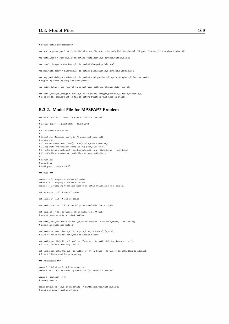
B.3. Model Files 169
# active paths per commodity
var active_paths_per_link {i in links} = sum {(m,n,k,i) in path_link_incidence} (if path_flow[m,n,k] > 0 then 1 else 0);
var total_hops = sum{(m,n,k) in paths} (path_cost[m,n,k]*used_path[m,n,k]);
var total_changes = sum {(m,n,k) in paths} changed_path[m,n,k];
var max_path_delay = max{(m,n,k) in paths} path_delay[m,n,k]*used_path[m,n,k];
var avg_path_delay = sum{(m,n,k) in paths} used_path[m,n,k]*path_delay[m,n,k]/active_paths;
# avg delay counting only the used paths;
var total_delay = sum{(m,n,k) in paths} used_path[m,n,k]*path_delay[m,n,k];
var total_cost_of_change = sum{(m,n,k) in paths} changed_path[m,n,k]*path_cost[m,n,k];
# cost of the change part of the objective function (not used in static).
B.3.2. Model File for MPSFAP2 Problem
### Model For Multicommodity Flow Allocation: MPSFAP
#
# Sergio Beker - INFRES-ENST - 03.03.2003
#
# File: MPSFAP.static.mod
#
# Objective: Minimize sum{p in P} path_cost*used_path
# subject to:
# 1) demand constraint: sum{p in Pq} path_flow = demand_q
# 2) capacity constraint: sum{p in Pi} path_flow <= Ci
# 3) path delay constraint: used_path*sum{i in p} link_delay <= max_delay
# 4) path flow constraint: path_flow <= used_path*limit
#
# variables:
# path_flow
# used_path : binary {0,1}
### SETS ###
param N > 0 integer; # number of nodes
param M > 0 integer; # number of links
param K > 0 integer; # maximun number of paths available for a couple.
set nodes := 1..N; # set of nodes
set links := 1..M; # set of links
set path_index := 1..K; # set of paths available for a couple.
set couples := {n1 in nodes, n2 in nodes : n1 <> n2};
# set of couples origin - destination
set path_link_incidence within {(m,n) in couples, k in path_index, i in links};
# path_link incidence matrix
set paths := setof {(m,n,k,i) in path_link_incidence} (m,n,k);
# list of paths in the path_link incidence matrix
set paths_per_link {i in links} := {(m,n,k,j) in path_link_incidence : i = j};
# list of paths traversing link i
set links_per_path {(m,n,k) in paths} := {j in links : (m,n,k,j) in path_link_incidence};
# list of links used by path (m,n,p)
### PARAMETERS ###
param C {links} >= 0; # link capacity
param e >= 0; # link capacity reduction (to avoid 0 division)
param d {couples} >= 0;
# demand matrix
param path_cost {(m,n,k) in paths} := card{links_per_path[m,n,k]};
# cost per path = number of hops

170 B. AMPL: A Modeling Language for Mathematical Programming
param B {(m,n,k) in paths} >= 0;
# a limit in the path_flow (to ensure used_path = 0 or 1)
param D {couples} >= 0;
# maximum delay to be admitted for a couple origin, destination
param previous_used_path {paths} binary;
### VARIABLES ###
var used_path {paths} binary; # path is used = 1, path is not used = 0
var changed_path {(m,n,k) in paths} = used_path[m,n,k]*(used_path[m,n,k]-previous_used_path[m,n,k]);
# path has changed = 1, paths has not changed = 0
var path_flow {paths} >= 0; # bp
var link_flow {i in links} = sum{(m,n,k,i) in paths_per_link[i]} path_flow[m,n,k];
# total flow in link i
var link_delay {i in links} = 1/(C[i]-link_flow[i]);
# link delay
var path_delay{(m,n,k) in paths} = sum{i in links_per_path[m,n,k]} link_delay[i];
# delay associated with a path
### OBJECTIVE ###
minimize total_cost : sum {(m,n,k) in paths} ((path_cost[m,n,k]+path_delay[m,n,k])*used_path[m,n,k]);
### CONSTRAINTS ###
subject to capacity_constraint {i in links}: link_flow[i] <= (1-e)*C[i];
# Capacity constraint
subject to path_flow_constraint {(m,n,k) in paths} : path_flow[m,n,k] <= B[m,n,k]*used_path[m,n,k];
# constraint to force used_paths to take values when b > 0
subject to demand_constraint {(m,n) in couples}: sum {(m,n,k) in paths} (path_flow[m,n,k]) = d[m,n];
# demand constraint
subject to delay_constraint {(m,n,k) in paths}: path_delay[m,n,k]*used_path[m,n,k] <= D[m,n];
# delay constraint per link
### CALCULATED VARIABLES TO DISPLAY ###
var avg_link_flow = sum{i in links} link_flow[i]/M;
var max_link_flow = max{i in links} link_flow[i];
var active_paths = sum{(m,n,k) in paths} (if path_flow[m,n,k] > 0 then 1 else 0);
# to see the total quantity of active paths;
var active_paths_per_commodity {(m,n) in couples} = sum{(m,n,k) in paths} (if path_flow[m,n,k] > 0 then 1 else 0);
# active paths per commodity
var active_paths_per_link {i in links} = sum {(m,n,k,i) in path_link_incidence} (if path_flow[m,n,k] > 0 then 1 else 0);
var total_hops = sum{(m,n,k) in paths} (path_cost[m,n,k]*used_path[m,n,k]);
var total_changes = sum {(m,n,k) in paths} changed_path[m,n,k];
var max_path_delay = max{(m,n,k) in paths} path_delay[m,n,k]*used_path[m,n,k];
var avg_path_delay = sum{(m,n,k) in paths} used_path[m,n,k]*path_delay[m,n,k]/active_paths;
# avg delay counting only the used paths;
var total_delay = sum{(m,n,k) in paths} used_path[m,n,k]*path_delay[m,n,k];
var total_cost_of_change = sum{(m,n,k) in paths} changed_path[m,n,k]*path_cost[m,n,k];
# cost of the change part of the objective function (not used in static).

B.3. Model Files 171
B.3.3. Model File for MTDFAP Problem
### Model For Multicommodity Flow Allocation: MTDFAP
#
# Sergio Beker - INFRES-ENST - 03.03.2003
#
# File: MTDFAP.mod
#
# Objective: Minimize sum{p in P} path_delay
# subject to:
# 1) demand constraint: sum{p in Pq} path_flow = demand_q
# 2) capacity constraint: sum{p in Pi} path_flow <= Ci
# 3) path delay constraint: used_path*sum{i in p} link_delay <= max_delay
# 4) path flow constraint: path_flow <= used_path*limit
#
# variables:
# path_flow
# used_path : binary {0,1}
### SETS ###
param N > 0 integer; # number of nodes
param M > 0 integer; # number of links
param K > 0 integer; # maximun number of paths available for a couple.
set nodes := 1..N; # set of nodes
set links := 1..M; # set of links
set path_index := 1..K; # set of paths available for a couple.
set couples := {n1 in nodes, n2 in nodes : n1 <> n2};
# set of couples origin - destination
set path_link_incidence within {(m,n) in couples, k in path_index, i in links};
# path_link incidence matrix
set paths := setof {(m,n,k,i) in path_link_incidence} (m,n,k);
# list of paths in the path_link incidence matrix
set paths_per_link {i in links} := {(m,n,k,j) in path_link_incidence : i = j};
# list of paths traversing link i
set links_per_path {(m,n,k) in paths} := {j in links : (m,n,k,j) in path_link_incidence};
# list of links used by path (m,n,p)
### PARAMETERS ###
param C {links} >= 0; # link capacity
param e >= 0; # link capacity reduction (to avoid 0 division)
param d {couples} >= 0;
# demand matrix
param path_cost {(m,n,k) in paths} := card{links_per_path[m,n,k]};
# cost per path = number of hops
param B {(m,n,k) in paths} >= 0;
# a limit in the path_flow (to ensure used_path = 0 or 1)
param D {couples} >= 0;
# maximum delay to be admitted for a couple origin, destination
param previous_used_path {paths} binary;
### VARIABLES ###
var used_path {paths} binary; # path is used = 1, path is not used = 0
var changed_path {(m,n,k) in paths} = used_path[m,n,k]*(used_path[m,n,k]-previous_used_path[m,n,k]);
# path has changed = 1, paths has not changed = 0
var path_flow {paths} >= 0; # bp
var link_flow {i in links} = sum{(m,n,k,i) in paths_per_link[i]} path_flow[m,n,k];
# total flow in link i

172 B. AMPL: A Modeling Language for Mathematical Programming
var link_delay {i in links} = 1/(C[i]-link_flow[i]);
# link delay
var path_delay{(m,n,k) in paths} = sum{i in links_per_path[m,n,k]} link_delay[i];
# delay associated with a path
### OBJECTIVE ###
minimize total_cost : sum {(m,n,k) in paths} (path_delay[m,n,k]*used_path[m,n,k]);
### CONSTRAINTS ###
subject to capacity_constraint {i in links}: link_flow[i] <= (1-e)*C[i];
# Capacity constraint
subject to path_flow_constraint {(m,n,k) in paths} : path_flow[m,n,k] <= B[m,n,k]*used_path[m,n,k];
# constraint to force used_paths to take values when b > 0
subject to demand_constraint {(m,n) in couples}: sum {(m,n,k) in paths} (path_flow[m,n,k]) = d[m,n];
# demand constraint
subject to delay_constraint {(m,n,k) in paths}: path_delay[m,n,k]*used_path[m,n,k] <= D[m,n];
# delay constraint per link
### CALCULATED VARIABLES TO DISPLAY ###
var avg_link_flow = sum{i in links} link_flow[i]/M;
var max_link_flow = max{i in links} link_flow[i];
var active_paths = sum{(m,n,k) in paths} (if path_flow[m,n,k] > 0 then 1 else 0);
# to see the total quantity of active paths;
var active_paths_per_commodity {(m,n) in couples} = sum{(m,n,k) in paths} (if path_flow[m,n,k] > 0 then 1 else 0);
# active paths per commodity
var active_paths_per_link {i in links} = sum {(m,n,k,i) in path_link_incidence} (if path_flow[m,n,k] > 0 then 1 else 0);
var total_hops = sum{(m,n,k) in paths} (path_cost[m,n,k]*used_path[m,n,k]);
var total_changes = sum {(m,n,k) in paths} changed_path[m,n,k];
var max_path_delay = max{(m,n,k) in paths} path_delay[m,n,k]*used_path[m,n,k];
var avg_path_delay = sum{(m,n,k) in paths} used_path[m,n,k]*path_delay[m,n,k]/active_paths;
# avg delay counting only the used paths;
var total_delay = sum{(m,n,k) in paths} used_path[m,n,k]*path_delay[m,n,k];
var total_cost_of_change = sum{(m,n,k) in paths} changed_path[m,n,k]*path_cost[m,n,k];
# cost of the change part of the objective function (not used in static).
B.3.4. Model File for MRPSFAP Problem
### Model For Multicommodity Flow Allocation: MINLP1a - Dynamic Formulation
#
# Sergio Beker - INFRES-ENST - 03.03.2003
#
# File: MINLP1a.dynamic.mod
#
# Objective: Minimize sum{p in P} path_cost*used_path + sum {p in P} path_cost*changed_path
# subject to:
# 1) demand constraint: sum{p in Pq} path_flow = demand_q
# 2) capacity constraint: sum{p in Pi} path_flow <= Ci
# 3) path delay constraint: used_path*sum{i in p} link_delay <= max_delay
# 4) path flow constraint: path_flow <= used_path*limit
# 5) change constraint: (used_path(t+1)-used_path(t))*used_path(t+1) <= changed_path(t+1)
#
# variables:
# path_flow
# used_path : binary {0,1}
# changed_path : binary {0,1}

B.3. Model Files 173
### SETS ###
param N > 0 integer; # number of nodes
param M > 0 integer; # number of links
param K > 0 integer; # maximun number of paths available for a couple.
set nodes := 1..N; # set of nodes
set links := 1..M; # set of links
set path_index := 1..K; # set of paths available for a couple.
set couples := {n1 in nodes, n2 in nodes : n1 <> n2};
# set of couples origin - destination
set path_link_incidence within {(m,n) in couples, k in path_index, i in links};
# path_link incidence matrix
set paths := setof {(m,n,k,i) in path_link_incidence} (m,n,k);
# list of paths in the path_link incidence matrix
set paths_per_link {i in links} := {(m,n,k,j) in path_link_incidence : i = j};
# list of paths traversing link i
set links_per_path {(m,n,k) in paths} := {j in links : (m,n,k,j) in path_link_incidence};
# list of links used by path (m,n,p)
### PARAMETERS ###
param C {links} >= 0; # link capacity
param e >= 0; # link capacity reduction (to avoid 0 division)
param d {couples} >= 0;
# demand matrix
param path_cost {(m,n,k) in paths} := card{links_per_path[m,n,k]};
# cost per path = number of hops
param B {(m,n,k) in paths} >= 0;
# a limit in the path_flow (to ensure used_path = 0 or 1)
param D {couples} >= 0;
# maximum delay to be admitted for a couple origin, destination
param previous_used_path {paths} binary;
### VARIABLES ###
var used_path {paths} binary; # path is used = 1, path is not used = 0
var changed_path {paths} binary;
# path has changed = 1, paths has not changed = 0
var path_flow {paths} >= 0; # bp
var link_flow {i in links} = sum{(m,n,k,i) in paths_per_link[i]} path_flow[m,n,k];
# total flow in link i
var link_delay {i in links} = 1/(C[i]-link_flow[i]);
# link delay
var path_delay{(m,n,k) in paths} = sum{i in links_per_path[m,n,k]} link_delay[i];
# delay associated with a path
### OBJECTIVE ###
minimize total_cost : sum {(m,n,k) in paths} (path_cost[m,n,k]*used_path[m,n,k]) + sum {(m,n,k) in paths} (path_cost[m,n,k]*changed_path[m,n,k]);
### CONSTRAINTS ###
subject to capacity_constraint {i in links}: link_flow[i] <= (1-e)*C[i];
# Capacity constraint
subject to path_flow_constraint {(m,n,k) in paths} : path_flow[m,n,k] <= B[m,n,k]*used_path[m,n,k];
# constraint to force used_paths to take values when b > 0

174 B. AMPL: A Modeling Language for Mathematical Programming
subject to demand_constraint {(m,n) in couples}: sum {(m,n,k) in paths} (path_flow[m,n,k]) = d[m,n];
# demand constraint
subject to delay_constraint {(m,n,k) in paths}: path_delay[m,n,k]*used_path[m,n,k] <= D[m,n];
# delay constraint per link
subject to path_change {(m,n,k) in paths} : (used_path[m,n,k]-previous_used_path[m,n,k])*used_path[m,n,k] <= changed_path[m,n,k];
### CALCULATED VARIABLES TO DISPLAY ###
var avg_link_flow = sum{i in links} link_flow[i]/M;
var max_link_flow = max{i in links} link_flow[i];
var active_paths = sum{(m,n,k) in paths} (if path_flow[m,n,k] > 0 then 1 else 0);
# to see the total quantity of active paths;
var active_paths_per_commodity {(m,n) in couples} = sum{(m,n,k) in paths} (if path_flow[m,n,k] > 0 then 1 else 0);
# active paths per commodity
var active_paths_per_link {i in links} = sum {(m,n,k,i) in path_link_incidence} (if path_flow[m,n,k] > 0 then 1 else 0);
var total_hops = sum{(m,n,k) in paths} (path_cost[m,n,k]*used_path[m,n,k]);
var total_changes = sum {(m,n,k) in paths} changed_path[m,n,k];
var max_path_delay = max{(m,n,k) in paths} path_delay[m,n,k]*used_path[m,n,k];
var avg_path_delay = sum{(m,n,k) in paths} used_path[m,n,k]*path_delay[m,n,k]/active_paths;
# avg delay counting only the used paths;
var total_cost_of_change = sum{(m,n,k) in paths} path_cost[m,n,k]*changed_path[m,n,k];
B.4. Data Files
B.4.1. Data File for MPSFAP and MTDFAP Problems
# NET2.dat
# Sergio Beker - ENST - INFRES: 27/01/03
#
# Multicommodity Flow Problem
# nodes = 4
# links = 10
# demands = 1.
# paths = 3 between nodes 1 and 4
data;
param e := 0.0001;
param D default 0.03;
param B default 10000;
param N := 4;
param M := 10;
param K := 5;
param C := 1 2500.0
2 2500.0
3 2500.0
4 2500.0
5 2500.0
6 2500.0
7 2500.0
8 2500.0
9 2500.0
10 2500.0
;
set path_link_incidence :=
(1,2,1,*) 1
(1,2,2,*) 9 4
(1,2,3,*) 8 6 4

B.4. Data Files 175
(1,3,1,*) 8
(1,3,2,*) 9 5
(1,3,3,*) 1 3 5
(1,4,1,*) 9
(1,4,2,*) 1 3
(1,4,3,*) 8 6
(2,1,1,*) 2
(2,1,2,*) 3 10
(2,1,3,*) 3 5 7
(2,3,1,*) 2 8
(2,3,2,*) 3 5
(2,3,3,*) 2 9 5
(2,3,4,*) 3 10 8
(2,4,1,*) 3
(2,4,2,*) 2 9
(2,4,3,*) 2 8 6
(3,1,1,*) 7
(3,1,2,*) 6 10
(3,1,3,*) 6 4 2
(3,2,1,*) 6 4
(3,2,2,*) 7 1
(3,2,3,*) 6 10 1
(3,2,4,*) 7 9 4
(3,4,1,*) 6
(3,4,2,*) 7 9
(3,4,3,*) 7 1 3
(4,1,1,*) 10
(4,1,2,*) 4 2
(4,1,3,*) 5 7
(4,2,1,*) 4
(4,2,2,*) 10 1
(4,2,3,*) 5 7 1
(4,3,1,*) 5
(4,3,2,*) 10 8
(4,3,3,*) 4 2 8
;
param previous_used_path default 0;
param d default 0.0 :
1 2 3 4 :=
1 . 346 729 1524
2 37 . 1186 1584
3 1477 1082 . 1834
4 1788 706 19 . ;
B.4.2. Data File for MRPSFAP Problem
# NET2.dat
# Sergio Beker - ENST - INFRES: 27/01/03
#
# Multicommodity Flow Problem
# nodes = 4
# links = 10
# demands = 1.
# paths = 3 between nodes 1 and 4
data;
param e := 0.0001;
param D default 0.03;
param B default 10000;

176 B. AMPL: A Modeling Language for Mathematical Programming
param N := 4;
param M := 10;
param K := 5;
param C := 1 2500.0
2 2500.0
3 2500.0
4 2500.0
5 2500.0
6 2500.0
7 2500.0
8 2500.0
9 2500.0
10 2500.0
;
set path_link_incidence :=
(1,2,1,*) 1
(1,2,2,*) 9 4
(1,2,3,*) 8 6 4
(1,3,1,*) 8
(1,3,2,*) 9 5
(1,3,3,*) 1 3 5
(1,4,1,*) 9
(1,4,2,*) 1 3
(1,4,3,*) 8 6
(2,1,1,*) 2
(2,1,2,*) 3 10
(2,1,3,*) 3 5 7
(2,3,1,*) 2 8
(2,3,2,*) 3 5
(2,3,3,*) 2 9 5
(2,3,4,*) 3 10 8
(2,4,1,*) 3
(2,4,2,*) 2 9
(2,4,3,*) 2 8 6
(3,1,1,*) 7
(3,1,2,*) 6 10
(3,1,3,*) 6 4 2
(3,2,1,*) 6 4
(3,2,2,*) 7 1
(3,2,3,*) 6 10 1
(3,2,4,*) 7 9 4
(3,4,1,*) 6
(3,4,2,*) 7 9
(3,4,3,*) 7 1 3
(4,1,1,*) 10
(4,1,2,*) 4 2
(4,1,3,*) 5 7
(4,2,1,*) 4
(4,2,2,*) 10 1
(4,2,3,*) 5 7 1
(4,3,1,*) 5
(4,3,2,*) 10 8
(4,3,3,*) 4 2 8
;
param previous_used_path [1,*,*] (tr)
: 2 3 4 :=
1 1 1 1
2 0 0 0
3 0 0 0
[2,*,*] (tr)
: 1 3 4 :=

B.4. Data Files 177
1 1 1 1
2 0 0 0
3 0 0 0
4 . 0 .
[3,*,*] (tr)
: 1 2 4 :=
1 1 1 1
2 0 1 0
3 0 0 0
4 . 0 .
[4,*,*] (tr)
: 1 2 3 :=
1 1 1 1
2 0 0 0
3 0 0 0
;
param d default 0.0 :
1 2 3 4 :=
1 . 346 1208 298
2 37 . 1186 1584
3 1477 1082 . 1834
4 1788 706 19 . ;


Bibliography
[1] R. Yavatkar, D. Pendarakis, R. Guerin, A Framework for Policy-based Admission Con-trol, RFC 2573, January 2000, IETF. 3.1.2
[2] D. Durham, J. Boyle, R. Cohen, S. Herzog, R. Rajan, A. Sastry, The COPS (CommonOpen Policy Service) Protocol, RFC 2748, January 2000, IETF. 3.1.2
[3] K. Chan, J. Seligson, D. Durham, S. Gai, K. McCloghrie, S. Herzog, F. Reichmeyer,R. Yavatkar, A. Smith, COPS Usage for Policy Provisioning (COPS-PR), RFC 3084,March 2001, IETF. 3.1.2
[4] R. Sahita, S. Hahn, K. Chan, K. McCloghrie, Framework Policy Information Base,RFC 3318, March 2003, IETF. 3.1.2
[5] S . Herzog, J. Boyle, R. Cohen, D. Durham, R. Rajan, A. Sastry, COPS usage forRSVP, RFC 2749, January 2000, IETF. 3.1.2
[6] D. Awduche, MPLS Traffic Engineering in IP Networks, IEEE Communications Mag-azine, December 1999, IEEE. 3, 3.1.1
[7] D. Awduche et al., Requirements for Traffic Engineering Over MPLS, RFC 2702,September 1999, IETF.
[8] R. Callon et al., A Framework for Multiprotocol Label Switching, Internet Draft, Septem-ber 1999, IETF. 3.1.3
[9] E. Rosen, A. Viswanathan, R. Callon, Multiprotocol Label Switching Architecture,RFC3031, January 2001, IETF. 3.1.3
[10] D. Awduche, L. Berger, D. Gan, T. Li, V. Srinivasan, G. Swallow, RSVP-TE: RSVPExtensions for MPLS Tunnels, RFC3209, December 2001, IETF. 3.3.1, 4.1, 7.3
[11] F. Le Faucheur, B. Davie, S. Davari, P. Vaanen, R. Krishnan, P. Cheval, J. Heinanen,Multiprotocol Label Switching (MPLS) Support for Differentiated Services, RFC3270,May 2002, IETF. 3.1.3, 4.7
[12] B. Jamoussi et al., Constraint-Based LSP Setup using LDP, RFC 3212, January 2002,IETF. 3.3.1, 4.1
179

180 Bibliography
[13] D. Awduche et al., RSVP-TE: Extensions to RSVP for LSP Tunnels, RFC 3209,December 2001, IETF.
[14] R.Ahuja, T.Magnanti, J.Orlin, Network Flows: Theory, Algorithms and Applications,Prentice Hall Inc., 1993, p.788-801. 4.6, A.1, A.3, A.4
[15] M.Kodialam, T.Lakshman, Minimum Interference Routing with Applications to MPLSTraffic Engineering, INFOCOM 2000, Proceedings IEEE, Volume 2. p.884-893. 3.3.1,4.8
[16] S.Beker, D.Kofman, N.Puech, Off-Line Reduced Complexity Layout Design for MPLSNetworks, Proceedings of IPOM 2003, p.99-105, IEEE. 4.3, 7.1
[17] S.Beker, D.Kofman, N.Puech, Off-Line MPLS Layout Design and Reconfiguration :Reducing Complexity Under Dynamic Traffic Conditions Proceedings of INOC 2003,p.61-66, ITC/INFORMS.
[18] J. Czyzyk, M. Mesnier, and J. More, The Neos Server, IEEE Journal on ComputationalScience and Engineering, 5, pages 68-75. 4.6.4
[19] R. Fletcher, S. Leyffer, Numerical Experience with Lower Bounds for MIQP Branchand Bound, SIAM Journal of Optimization, 8(2):p.604-616, 1998. 4.6.4
[20] Roberts J.W., Self-Similar Network Traffic and Performance Evaluation, chapter En-gineering for Quality of Service, Wiley-Interscience, 2000, pages 401-420. 4.2
[21] Cabinet Arcome, Etude Technique, Economique et Reglamentaire de l’Evolution versles Reseaux de Nouvelle Generation, Autoritede Regulation des Telecommunications,Septembre 2000. 2.3.3, 2.3.4
[22] E. Altman, T. Basar, T. Jimenez, N. Shimkin, Competitive Routing in Networks withPolynomial Costs, INFOCOM 2000, Proceedings IEEE, Volume 3, p.1586-1593. 4.1,4.3, 4.8
[23] L. Georgiadis, K. Floros, P. Georgatsos, S. Sartzetakis, Lexicographically OptimalBalanced Networks, INFOCOM 2001, Proceedings IEEE, Volume 2, p.689-698. 4.1, 4.3,4.8
[24] H. Hsu, F. Yeang-Sung Lin, Near-Optimal Constrained Routing in Virtual CircuitNetworks, INFOCOM 2001, Proceedings IEEE, Volume 2, p.750-756. 4.1, 4.3, 4.8
[25] D. Banerjee, B. Mukherjee, Wavelength-Routed Optical Networks: Linear Formulation,Resource Budgeting Tradeoffs, and a Reconfiguration Study, Networking, IEEE/ACMTransactions on, Volume: 8 Issue: 5 , Oct 2000, p.598-607. 3.3.1, 4.1, 4.6.1, 7.1, 7.6.1

Bibliography 181
[26] G. Banerjee, D. Sidhu, Path Computation for Traffic Engineering in MPLS Networks,Proceedings of IEEE ICN 2001.
[27] A. Feldman, A.C. Gibert, P. Huang, W. Willinger, Dynamics of IP Traffic: A Studyof the Role of Variability and the Impact of Control, SIGCOM 1999. 4.2
[28] M. Nabe, M. Murata, H. Miyahara, Analysis and Modeling of Worldwide Web Trafficfor Capacity Dimensioning of Internet Access Lines Performance Evaluation, (34):249-271, 1998. 4.2
[29] K. Thompson, G.J. Miller, R. Wilder, Wide-Area Internet Traffic Patterns and Char-acterization, IEEE Network, Nov/Dec. 1997, pages: 10-23. 4.2
[30] L. Kleinrock, Queueing systems, Vol. 1 : Theory, John Wiley & Sons, New York, USA.1975. 4.3
[31] L. Kleinrock, Queueing systems, Vol. 2 : Computer Applications, John Wiley & Sons,New York, USA. 1976. 5.1, 8.5
[32] T. Wang, Global Optimization for Constrained Non Linear Programming, PhD. Thesis,University of Illinois at Urbana-Champaign, 2001. 4.6
[33] Michael R. Garey, David. S. Johnson, Computers and Intractability: A Guide to theTheory of NP-Completeness, W. H. Freemand and Co. New York, 1979. 4.6
[34] George L. Nemhouser, Laurence A. Walsey, Integer and Combinatorial Optimization,John Wiley & Sons, New York, 1988. 4.6
[35] M. Ajmone Marsan, A. Grosso, E. Leonardi, M. Mellia, A. Nucci, Design of LogicalTopologies in Wavelength-Routed IP Networks, Photonic Network Communications,December 2002, Vol.4, No.3/4, pp.423-442, ISSN: 1387-974x. 4.6
[36] Robert Fourer, David M. Gay, Brian W. Kernighan, AMPL: A Modeling Languagefor Mathematical Programming, Second Edition, Thompson, Brooks/Cole, USA, 2003.4.6.4, B.1, B.1
[37] W. Gropp and J. More, Optimization Environments and the NEOS Server, Approxi-mation Theory and Optimization, M. D. Buhmann and A. Iserles, eds., pages 167-182,1997, Cambridge University Press. 4.6.4
[38] E. Dolan, The NEOS Server 4.0 Administrative Guide, Technical MemorandumANL/MCS-TM-250, Mathematics and Computer Science Division, Argonne NationalLaboratory, May 2001. 4.6.4
[39] R. Fletcher, S. Leyffer, User Manual for Filter SQP, Numerical Analysis Report,NA/181, Dundee University, April, 1998. 4.6.4

182 Bibliography
[40] W. Ben-Ameur, B. Liau, N. Michel, Routing Strategies for IP Networks, 2/3 2001,Telektronik Magazine, p. 145-158. 3.1.3, 4.8, 6.2
[41] S. C. Erbas, R. Mathar:, An Off-line Traffic Engineering Model for MPLS Networks,Proceddings of IEEE 27th Annual IEEE Conference on Local Computer Networks (27thLCN), pp. 166-174, Tampa, Florida, November 2002.
[42] M. Pioro, A. Myslek, Topological Design of MPLS Networks, IEEE GLOBECOM 2001,San Antonio, Texas, 2001. 4.1
[43] D. Bienstock, S. Chopra, O. Guenluek, C.Y. Tsai, Minimum Cost Capacity Installationfor Multicommodity Network Flows, Mathematical Programming Journal, (81), p.177-199, 1998. 4.1
[44] N. Geary, A. Antonopoulos, E. Drakopoulos, J. O’Reilly, Analysis Of OptimisationIssues In Multi-Period DWDM Network Planning, IEEE INFOCOM 2001, Anchorage,Alaska, p.152-158. 4.1
[45] B. Fortz, M. Thorup, Internet Traffic Engineering by Optimizing OSPF Weights, IEEEINFOCOM, p.519-528, 2000. 3.1.2, 3.1.3, 4.8, 7.1
[46] F. Ergun, R. Sinha, L. Zhang, QoS Routing with PerformanceDependent Costs, IEEEINFOCOM, 2000. 4.8
[47] A. Orda, A. Sprintson, QoS Routing: The Precomputation Perspective, IEEE INFO-COM, p.128-136, 2000. 4.8
[48] T. Korkmaz, M. Krunz, Multi-Constrained Optimal Path Selection, IEEE INFOCOM,p.834-843, 2001. 4.8
[49] A. Juttner, B. Szviatovszki, I. Mecs, Z. Rajko, Lagrange Relaxation Based Method forthe QoS Routing Problem, IEEE INFOCOM, 2001. 4.8
[50] A. Goel, K.G. Ramakrishnan, D. Kataria, D. Logothetis, Efficient Computation ofDelay-sensitive Routes from One Source to All Destinations, IEE INFOCOM, p.854-858, 2001. 4.8
[51] O.K. Gupta, A. Ravindran, Branch and Bound Experiments in Convex Non-LinearInteger Programming, Management Science, 31(12), p.1533-1546, 1985. 5.1
[52] I. Quesada, I.E. Grossmann, An LP/NLP Based Branch and Bound Algorithm forConvex MINLP Optimization Problems, Computers Chemical Engineering, 16(10/11),p.937-947, 1992. 5.1
[53] A.M. Geoffrion, A Generalized Benders Decomposition, Journal on Optimization The-ory and Applications, 10(4), p.237-260, 1972. 5.1

Bibliography 183
[54] M.A. Duran, I.E. Grossmann, An Outer-Approximation Algorithm for a Class of Mixed-Integer Non-Linear Programming, Mathematical Pogramming, 36, p.307-339, 1986.5.1
[55] R. Fletcher, S. Leyffer, Solving Mixed Integer Programs by Outer Approximation,Mathematical Pogramming, 66, p.327-349, 1994. 5.1
[56] S. Leyffer, Integrating SQP and branch-and-bound for Mixed Integer Nonlinear Pro-gramming, Computational Optimization and Applications, 18, p.295-309, 2001. 5.1
[57] T. Westerlund, F. Petersson, A Cutting Plane Method for Solving Convex MINLPProblems, Computers Chemical Engineering, 19, p.131-136, 1995. 5.1
[58] S. Kirkpatrick, C.D. Gelatt Jr.,M.P. Vecchi, Optimization by Simulated Annealing,Science Journal, number 4598, 1983. 5.2
[59] C. Gazen, C. Ersoy, Genetic algorithms for designing multihop lightwave networktopologies, Artificial Intelligence in Engineering, (3), p.211-221, 1999. 5.2
[60] F. Glover, M. Laguna, Tabu Search, Kluwer Academic Publishers, 1997, Boston, MA.5.2
[61] N. Puech, J. Kuri, M. Gagnaire, Models for the Logical Topology Design Problem,Proceedings of the 2nd IFIP-TC6 Networking Conference, May, 2002, Springer-Verlag.5.2
[62] S. Beker, N. Puech, V. Friderikos, A Tabu Search Heuristic for the Off-Line MPLSReduced Complexity Layout Design Problem, IFIP-TC6 Networking Conference 2004,LNCS Springer Verlag Networking 2004 (to be published) May 9-14, Athens. 5.3
[63] Reseau National de Reherche en Teleommunications, 2000-2004, Ministere del’Economie, des Finances et de l’Industrie, France, www.vthd.org. 1, 6.1
[64] D. Bertsekas, R. Gallager, Data Networks, Prentice-Hall International Editions, UK,1987. 3.1.2, 5.1, 5.4.1, 5.4.1, 5.5, 8.5
[65] J.E. Burns, T.J. Ott, Johan M. de Kock, A.E. Krzesinski, Path Selection and BandwidthAllocation in MPLS Networks: a Non-Linear Programming Approach, Proceedings ofSPIE, ITCom (4523), 2001. 5.1, 5.5, 1, 5.5
[66] A. Kershenbaum, Telecommunication Design Algorithms, McGraw-Hill, 1993.
[67] L. Fratta, M. Gerla, L. Kleinrock, The Flow Deviation Method: An Approach to Store-and-Forward Communication Network Design, Networks, (3), p.97-133, 1973. 5.4,5.4.1

184 Bibliography
[68] M. Lucas, D. Wrege, B. Dempsey, A. Weaver, Statistical Characterization of Wide-AreaIP Traffic, Sixth International Conference on Computer Communications and Networks(IC3N’97), Las Vegas, NV, September 1997. (document), 7.1, 7.2, 7.1
[69] T. Bonald, S. Oueslati-Boulahia, J.W. Roberts, IP traffic and QoS control: the needfor a flow-aware architecture, World Telecommunications Congress, September 2002Paris, France. (document), 7.1, 7.2, 7.2
[70] A. Genata, B. Mukherjee, Virtual-Topology Adaptation for WDM Lesh Networks UnderDynamic Traffic, INFOCOM 2002, Proceedings IEEE, (1) p.48-56, 2002. 7.1
[71] B. Ramamurthy, A. Ramakrishnan, Virtual Topology Reconfiguration of Wavelength-Routed Optical WDM Networks, GLOBECOM 2000, Proceedings IEEE, (2) p.1269-1275, 2000. 7.1
[72] F. Ricciato, S. Salsano, A. Belmonte, M. Listanti, Off-Line Configuration of a MPLSover WDM Network under Time-Varying Offered Traffic, INFOCOM 2002, ProceedingsIEEE, (1) p.57-65, 2002. 7.1
[73] W. Ben-Ameur, H. Kerivin, Routing of uncertain demands, submitted to Journal onOperations Research, 2001. 7.1
[74] J.F.P. Labourdette, G.W.Hart, A.S.Acampora, Branch-Exchange Sequences for Re-configuration of Lightwave Networks, IEEE Transactions on Communications, 42(10)p.2822-2832, October 1994. 7.1
[75] B. Fortz, J. Rexford, M. Thorup, Traffic Engineering with Traditional IP RoutingProtocols, IEEE Communications Magazine, 2002. 3.1.3, 7.1
[76] R. Casellas, Tesis, ENST, 2002. 3.1.2
[77] K. Ramakrishnan, S. Floyd, D. Black, The Addition of Explicit Congestion Notification(ECN) to IP, RFC 3178, IETF, Septemnber 2001. 3.1.2
[78] K. Ishiguro, T. Takada, Traffic Engineering Extensions to OSPF version 3, Draft(draft-ietf-ospf-ospfv3-traffic-01.txt), IETF. August 2003. 3.1.3
[79] S. Blake, D. Black, M. Carlson, E. Davies, Z. Wang, W. Weiss An Architecture forDifferentiated Services, RFC 2475, IETF, August 1998. 3.1.3
[80] J. Wroclawski, The Use of RSVP with IETF Integrated Services, RFC 2210, IETF,September 1997. 3.1.3
[81] D. Grossman, New Terminology and Clarifications for Diffserv, RFC 3260, IETF,April 2002. 3.1.3

Bibliography 185
[82] M. Grossglauser, J. Rexford, Passive Traffic Measurement for IP Operations, TheInternet as a Large-Scale Complex System (Chapter), Oxford University Press, toappear 2004. 3.2.1
[83] V. Paxson, G. Almes, J. Mahdavi, M. Mathis, Framework for IP Performance Metrics,RFC 2330, IETF, May 1998. 3.2.1
[84] E. Castillo, A.J. Conejo, P. Pedregal, R. Garcia, N. Alguacil, Building and SolvingMathematical Programming Models in Engineering and Science, ISBN: 0-471-15043-6,Hardcover, 568 pages, October 2001. 4.6.4, B.1
[85] A. Feldman, A. Greenberg, C. Lund, N. Reingold, J. Rexford, F. True, Deriving TrafficDemands for Operational IP Networks: Methododoly and Experience, Proceedings ofACM SIGCOM 2000, , 2000. 4.2
[86] B. Krithikaivasan, K. Deka, D. Medhi, Adaptive Bandwidth Provisioning EnvelopeBased on Discrete Temporal Network Measurements, Proceedings of IEEE INFOCOM2004, Hong Kong, March 2004. 4.2
[87] K. Papagiannaki, N. Taft, Z.L. Zhang, C. Diot, Long-term Forecasting of InternetBackbone Traffic: Observations and Initial Models, Proceedings of IEEE INFOCOM2003, San Francisco, CA, March 2003. 4.2
[88] S. Srivastava, B. Krithikaivasan, D. Medhi, M. Pioro, Traffic Engineering in the Pres-ence of Tunneling and Diversity Constraints: Formulation and Lagrangian Decomposi-tion Approach, Proceedings of 18th International Teletraffic Congress (ITC18), pages461-470, September 2003. 4.8
[89] B. Yaged, Minimum Cost Routing for Dyanamic Network Models, Networks, 3:193-224,1973. 7.1
[90] N. Zadeh, On Building Minimum Cost Communication Networks Over Time, Net-works, 4:19-34, 1974. 7.1