optimization problems in mobile comm
TRANSCRIPT

DISS. ETH No. 16207, 2005
Optimization Problems inMobile Communication
A dissertation submitted to theSwiss Federal Institute of Technology, ETH Zurichfor the degree of Doctor of Technical Sciences
presented byDipl. Eng. in Comp. Sc. Gabor Vilmos Szaboborn 19.12.1976, citizen of Zalau, Romania
accepted on the recommendation ofProf. Dr. Peter Widmayer, ETH Zurich, examinerDr. Thomas Erlebach, University of Leicester, co–examinerDr. Riko Jacob, ETH Zurich, co–examiner


Katibogaramnak

Abstract
In one way or another mobile phones have changed everyone’s life.Mobile communication networks made it possible to be connectedand reachable even in the most remote places. A lot of research ef-fort has been put lately in the planning and optimization of mobilenetworks. Network providers as well as users can only gain in effi-ciency and usability if the algorithmic optimization community pro-vides them with efficient algorithmic solutions to the optimizationproblems raised by mobile communication networks.
In this thesis, we analyze three different algorithmically interest-ing problems stemming from mobile telecommunication: the basestation location with frequency assignment; the OVSF code assign-ment problem; and the joint base station scheduling problem.
We propose a new solution technique to the problem of position-ing base station transmitters and assigning frequencies to the trans-mitters. This problem stands at the core of GSM network designand optimization. Since most interesting versions of this problem areNP-hard, we follow a heuristic approach based on the evolutionaryparadigm to find good solutions. We examine and compare two stan-dard multiobjective techniques and a new algorithm, the steady stateevolutionary algorithm with Pareto tournaments (stEAPT). The evo-lutionary algorithms used raised an interesting data structure prob-lem. We present a fast priority queue based technique to solve thelayers-of-maxima problem arising in the evolutionary computation.The layers-of-maxima problem asks to partition a set of points ofsize n into layers based on their non-dominatedness. A point in d-dimensional space is said to dominate another point if it is not worsethan the other point in all of the d dimensions.
We also look at the problem of dynamically allocating OVSFcodes to users in an UMTS network. The combinatorial core of theOVSF code assignment problem is to assign some nodes of a com-plete binary tree of height h (the code tree) to n simultaneous con-nections, such that no two assigned nodes (codes) are on the sameroot-to-leaf path. A connection that uses 2−d of the total bandwidthrequires an arbitrary code at depth d in the tree. This code assignmentis allowed to change over time, but we want to keep the number ofcode changes as small as possible. We consider the one-step code as-signment problem: Given an assignment, move the minimum number

ii
of codes to serve a new request. We show that the problem is NP-hard. We give an exact nO(h)-time algorithm, and a polynomial timegreedy algorithm that achieves approximation ratio Θ(h). A morepractically relevant version is the online code assignment problem.Our objective is to minimize the overall number of code reassign-ments. We present a Θ(h)-competitive online algorithm. We givea 2-resource augmented online-algorithm that achieves an amortizedconstant number of assignments.
The joint base station scheduling problem (JBS) arises in UMTSnetworks. Consider a scenario where radio base stations need to senddata to users with wireless devices. Time is discrete and slotted intosynchronous rounds. Transmitting a data item from a base station to auser takes one round. A user can receive the data item from any of thebase stations. The positions of the base stations and users are mod-eled as points in Euclidean space. If base station b transmits to user uin a certain round, no other user within distance ‖b − u‖2 from b canreceive data in the same round due to interference phenomena. Giventhe positions of the base stations and of the users the goal is to mini-mize the number of rounds necessary to serve all users. We considerthis problem on the line (1D-JBS) and in the plane (2D-JBS). For 1D-JBS, we give an efficient 2-approximation algorithm and polynomialtime optimal algorithms for special cases. We also present an exactalgorithm for the general 1D-JBS problem with exponential runningtime. We model transmissions from base stations to users as arrows(intervals with a distinguished endpoint) and show that their conflictgraphs, which we call arrow graphs, are a subclass of perfect graphs.For 2D-JBS, we prove NP-hardness and show lower bounds on theapproximation ratio of some natural greedy heuristics.

iii
Zusammenfassung
Auf die eine oder andere Art hat Mobilfunk viele Menschen beein-flusst. Mobilfunknetzwerke haben es ermoglicht, selbst in den abgele-gensten Orten erreichbar zu sein. In letzter Zeit wurde viel Forschungin die Planung und Optimierung von Mobilfunknetzwerken investiert.Netzwerkanbieter und Nutzer konnen nur davon profitieren, wenn Al-gorithmiker effiziente Losungen fur Optimierungsprobleme aus die-sem Umfeld liefern.
In dieser Dissertation analysieren wir drei verschiedene algorith-misch interessante Probleme der mobilen Telekommunikation: Funk-mastplatzierung mit Frequenzzuweisung, OVSF Code Zuweisung undJoint Base Station Scheduling.
Wir prasentieren eine neuartige Losungstechnik fur das Problem,Funkmasten zu positionieren und ihnen Frequenzen zuzuordnen. Die-se Fragestellung ist ein Kernproblem beim Design und der Optimie-rung von GSM Netzwerken. Da die interessanteste Version diesesProblems NP-hart ist, benutzen wir einen heuristischen Ansatz, derauf dem evolutionaren Paradigma beruht, um gute Losungen zu fin-den. Wir untersuchen und vergleichen zwei multikriterielle Techni-ken und einen neuen Algorithmus, den ,,steady state” evolutionarenAlgorithmus mit Pareto Turnieren (stEAPT). Die evolutionaren Al-gorithmen, die hier benutzt werden, werfen ein interessantes Daten-strukturen Problem auf. Wir stellen eine auf Prioritatswarteschlangenbasierende Technik vor, die das entstehende ,,Maxima-Schichten” Pro-blem lost. Dieses Problem besteht darin, eine Menge von Punkten derGroße n so in Schichten aufzuteilen, dass sich keine zwei Punkte ineiner Schicht dominieren. Hierbei dominiert ein Punkt in Rd einenanderen, wenn er in keiner Dimension schlechter ist als der andereund in mindestens einer besser.
Weiterhin betrachten wir das Problem, dynamisch OVSF Codes ineinem UMTS Netzwerk zu allozieren. Der kombinatorische Kern desOVSF Code Zuweisungsproblems besteht darin, Knoten eines voll-standigen binaren Baums der Hohe h (Codebaum) n gleichzeitigenVerbindungen zuzuweisen, so dass keine zwei zugewiesenen Codesauf einem Wurzel-Blatt Pfad sind. Eine Verbindung, die einen Anteilvon 2−d der zu Verfugung stehenden Bandbreite benotigt, brauchteinen beliebigen Code der Tiefe d im Baum. Diese Codezuweisungkann sich mit der Zeit andern. Dabei wollen wir die Anzahl der Code-
iv
Neuzuweisungen moglichst klein halten. Wir betrachten das Ein-Schritt Codezuweisungsproblem: Gegeben eine Codezuweisung, be-wege die minimale Anzahl von Codes, um die neue Anfrage zu bedie-nen. Wir zeigen, dass dieses Problem NP-vollstandig ist. Wir stelleneinen exakten nO(h) Zeit Algorithmus vor und einen polynomiellen,,Greedy”-Algorithmus mit Approximationsrate Θ(h). Eine praktischrelevantere Variante ist das Online-Codezuweisungsproblem: Mini-miere die Zahl der Codezuweisungen uber eine (unbekannte) Anfra-gesequenz. Dafur prasentieren wir einen Θ(h)-kompetitiven Algo-rithmus. Schließlich stellen wir einen 2-,,Ressourcen-augmentierten”Online Algorithmus vor, der eine amortisiert konstante Anzahl vonZuweisungen benotigt.
Das Problem des verbundenen Funkmast Scheduling (JBS) ent-steht in UMTS Netzwerken. Betrachten wir ein Szenario, in demFunkmasten Daten an Benutzer mit Mobilgeraten senden. In unseremModell betrachten wir die Zeit diskretisiert und synchron in Rundensegmentiert. Die Ubertragung eines Datenpakets vom Funkmastenzum Benutzer benotigt eine Runde. Ein Benutzer kann ein Daten-paket von einem beliebigen Funkmasten erhalten. Die Position desFunkmasten und des Benutzers modellieren wir als Punkte in der eu-klidischen Ebene. Wenn Funkmast b an Benutzer u in einer bestimm-ten Runde sendet, kann wegen Interferenz kein Benutzer innerhalbeiner Distanz von ‖b − u‖2 von b in der gleichen Runde Daten emp-fangen. Fur gegebene Positionen von Funkmasten und Benutzern be-steht die Aufgabe darin, die Anzahl der Runden zu minimieren, bisalle Benutzer ihre Daten erhalten haben. Dieses Problem betrachtenwir auf der Geraden (1D-JBS) und in der Ebene (2D-JBS). Fur 1D-JBS prasentieren wir einen effizienten 2-Approximationsalgorithmusund Polynomialzeitalgorithmen fur Spezialfalle. Weiterhin stellen wireinen exakten Algorithmus fur 1D-JBS mit exponentieller Laufzeitvor. Ubertragungen vom Funkmasten zu den Benutzern werden imEindimensionalen als Pfeile dargestellt. Wir zeigen, dass die entste-henden Konfliktgraphen, die wir ,,arrow graphs” nennen, eine Sub-klasse der Perfekten Graphen sind. Fur 2D-JBS zeigen wir NP-Voll-standigkeit und untere Schranken fur die Approximierbarkeit einigerGreedy-Heuristiken.

v
Acknowledgment
No thesis is ever the product of only one person’s efforts, and cer-tainly this one was no exception. It would never have become real-ity without the help and suggestions of my advisors, colleagues andfriends.
First of all I would like to thank my supervisor prof. Peter Wid-mayer for his constant guidance, support and for his thoughtful andcreative comments.
I am also very grateful to my co-examiners Dr. Thomas Erlebachand Dr. Riko Jacob for reading my thesis and for working with meon some of the challenging algorithmic problems presented in thispiece of work. I would also like to express many thanks to my coau-thors Matus Mihalak, Marc Nunkesser, Karsten Weicker and NicoleWeicker for the brainstorming hours and also for the fun we had atconferences. In this regard, I am also indebted to Michael Gatto forsharing the office with me for the past two years, for being such agreat colleague, for proof reading my thesis as well as for the discus-sions on photography and many other topics.
I would also like to take this opportunity to thank many people andfriends with whom I spent time, academically and socially. I thankDr. Christoph Stamm for giving me advice on good programmingstyle and also for being my supervisor during my diploma work. Aspecial thank you goes to Barbara Heller who always helped me whenI needed advice regarding the academic life at the ETH and life inZurich. I am also grateful to my former and current colleagues fortheir friendship: Luzi Anderegg, Dr. Mark Cieliebak, Jorg Derungs,Dr. Stephan Eidenbenz, Dr. Alex Hall, Dr. Tomas Hruz, ZsuzsannaLiptak, Dr. Sonia P. Mansilla, Dr. Leon Peeters, Dr. Paolo Penna,Conrad Pomm, Dr. Guido Proietti, Franz Roos, Konrad Schlude, Dr.David Taylor and Mirjam Wattenhofer. In this respect I would alsolike to thank my Hungarian and Romanian friends from the ETH fororganizing the numerous parties and many other social events.
I am also grateful to my parents for their support and encourage-ment during these five years.
My biggest thank you goes to Veronika Bobkova who alwaysmade me motivated when I was loosing faith in my work and forsupporting me.

vi

Contents
1 Introduction 1
1.1 GSM and UMTS System Planning and Optimization 2
1.2 Short Theory of Algorithms and Complexity . . . . . 5
1.3 Summary of Results . . . . . . . . . . . . . . . . . . 10
2 Base Station Placement with Frequency Assignment 15
2.1 Introduction . . . . . . . . . . . . . . . . . . . . . . 15
2.1.1 Related Work . . . . . . . . . . . . . . . . . 16
2.1.2 Model and Notation . . . . . . . . . . . . . 17
2.1.3 Summary of Results . . . . . . . . . . . . . 20
2.2 Design Criteria and Multiobjective Methods . . . . . 22
2.3 Concrete Realization . . . . . . . . . . . . . . . . . 25
2.3.1 Repair Function . . . . . . . . . . . . . . . . 25
2.3.2 Initialization . . . . . . . . . . . . . . . . . 26
2.3.3 Mutation . . . . . . . . . . . . . . . . . . . 26
2.3.4 Recombination . . . . . . . . . . . . . . . . 28
2.3.5 Selection . . . . . . . . . . . . . . . . . . . 29
2.3.6 Algorithm . . . . . . . . . . . . . . . . . . . 33
2.4 Experiments . . . . . . . . . . . . . . . . . . . . . . 35
2.4.1 Experimental Setup . . . . . . . . . . . . . . 35
2.4.2 Statistical Comparison . . . . . . . . . . . . 36
2.4.3 Parameter Settings . . . . . . . . . . . . . . 37
2.4.4 Multiobjective Methods . . . . . . . . . . . 38
i

ii Contents
2.5 Conclusions and Open Problems . . . . . . . . . . . 39
3 Maxima Peeling in d-Dimensional Space 49
3.1 Introduction . . . . . . . . . . . . . . . . . . . . . . 49
3.1.1 Related Work . . . . . . . . . . . . . . . . . 51
3.1.2 Model and Notation . . . . . . . . . . . . . 52
3.1.3 Summary of Results . . . . . . . . . . . . . 52
3.2 Sweep-Hyperplane Algorithm . . . . . . . . . . . . 54
3.2.1 The Layer-of-Maxima Tree . . . . . . . . . . 54
3.2.2 Space and Running Time Analysis . . . . . . 59
3.3 Divide and Conquer Algorithm . . . . . . . . . . . . 61
3.3.1 Algorithm . . . . . . . . . . . . . . . . . . . 61
3.3.2 Space and Running Time Analysis . . . . . . 65
3.4 Semi-Dynamic Set of Maxima . . . . . . . . . . . . 70
3.5 Conclusions and Open Problems . . . . . . . . . . . 73
4 OVSF Code Assignment 75
4.1 Introduction . . . . . . . . . . . . . . . . . . . . . . 75
4.1.1 Related Work . . . . . . . . . . . . . . . . . 77
4.1.2 Model and Notation . . . . . . . . . . . . . 78
4.1.3 Summary of Results . . . . . . . . . . . . . 79
4.2 Properties of OVSF Code Assignment . . . . . . . . 81
4.2.1 Feasibility . . . . . . . . . . . . . . . . . . . 81
4.2.2 Irrelevance of Higher Level Codes . . . . . . 82
4.2.3 Enforcing Arbitrary Configurations . . . . . 83
4.3 One-Step Offline CA . . . . . . . . . . . . . . . . . 86
4.3.1 Non-Optimality of Greedy Algorithms . . . 86
4.3.2 NP-Hardness . . . . . . . . . . . . . . . . 87
4.3.3 Exact nO(h) Algorithm . . . . . . . . . . . 90
4.3.4 h-Approximation Algorithm . . . . . . . . . 92
4.4 Online CA . . . . . . . . . . . . . . . . . . . . . . . 98
4.4.1 Compact Representation Algorithm . . . . . 99
4.4.2 Greedy Online Strategies . . . . . . . . . . . 101

Contents iii
4.4.3 Minimizing the Number of Blocked Codes . 102
4.4.4 Resource Augmented Online Algorithm . . . 106
4.5 Discussions and Open Problems . . . . . . . . . . . 108
5 Joint Base Station Scheduling 109
5.1 Introduction . . . . . . . . . . . . . . . . . . . . . . 109
5.1.1 Related Work . . . . . . . . . . . . . . . . . 110
5.1.2 Model and Notation . . . . . . . . . . . . . 112
5.1.3 Summary of Results . . . . . . . . . . . . . 115
5.2 1D-JBS . . . . . . . . . . . . . . . . . . . . . . . . 116
5.2.1 Relation to Other Graph Classes . . . . . . . 116
5.2.2 1D-JBS with Evenly Spaced Base Stations . 118
5.2.3 3k Users, 3 Base Stations in k Rounds . . . . 121
5.2.4 Exact Algorithm for the k-Decision Problem 122
5.2.5 Approximation Algorithm . . . . . . . . . . 125
5.2.6 Different Interference Models . . . . . . . . 128
5.3 2D-JBS . . . . . . . . . . . . . . . . . . . . . . . . 130
5.3.1 NP-Completeness of the k-2D-JBS Problem 130
5.3.2 Base Station Assignment for One Round . . 141
5.3.3 Approximation Algorithms . . . . . . . . . . 143
5.4 Conclusions and Open Problems . . . . . . . . . . . 149

iv Contents

Chapter 1
Introduction
In one way or another mobile phones have changed everyone’s life.We can say that nowadays more than half of the population has amobile phone or at least has used a mobile phone. Mobile communi-cation networks made it possible to be connected and reachable evenin the most remote places. One might question whether this is goodor bad. The truth is mobile phones can nowadays save lives but theelectro-smog can also endanger life if not kept below the allowedlimits. Since predictions show that in future most of the communica-tion will be in the mobile domain (maybe even the internet), it makessense to optimize mobile networks for the most efficient utilization ofthe frequency spectrum and for minimizing smog.
Both the telecommunication network providers and the users canonly gain in efficiency and usability if we theoreticians provide themwith the most efficient algorithmic solutions to all interesting prob-lems raised by these networks. While there exist a number of re-sults on several aspects of telecommunication network planning andmanagement, very little is known about models that use a holistic ap-proach trying to take all aspects into account at the same time. Mosttheoretical problems in telecommunications turn out to be NP-hard,which makes the existence of efficient polynomial-time algorithmsthat find optimum solutions highly unlikely. The notion of approxi-mation algorithms was introduced for such situations. Approximationalgorithms are algorithms that run in polynomial time and find solu-tions that are guaranteed to be at most a certain factor (i.e., a constant
1

2 Chapter 1. Introduction
or a function of the input size) off the optimum solution. This con-trasts with the concept of a heuristic, where no such guarantee canbe given, but good solutions are found for most instances arriving inpractice. In practice, heuristics often outperform ”provably”worst-case optimum approximation algorithms.
From a practical point of view, mobile phones affect all of us.New mobile phone networks are being designed for each new tech-nology generation. Each generation poses a different set of problems.When designing new networks, algorithmically challenging and com-putationally intensive problems without existing theoretical modelshave to be solved. In this thesis we elaborate on three of these chal-lenging problems: coverage and frequency allocation (in Chapter 2),spreading code allocation (in Chapter 4), and load balancing with cellsynchronization (in Chapter 5). In addition we analyze a data struc-ture problem (in Chapter 3) that improves the runtime efficiency of aclass of evolutionary multi-objective optimization strategies.
First, we present shortly some aspects of the design and optimiza-tion problems raised by 2nd and 3rd generation mobile telecommu-nication networks. For a technical description on the existing andfuture generation mobile networks, the interested reader is referredto [76, 46] and [60]. Next, we present briefly the algorithmic toolsand theory used for solving and analyzing the problems tackled inthis thesis. At the end of this chapter we present our main resultsand in the following chapters we present in detail each of the abovementioned problems.
1.1 GSM and UMTS System Planning andOptimization
Global System for Mobile communication (GSM) is the current mostwidely spread digital cellular mobile communication standard. Its ra-dio interface is based on Frequency Division Multiple Access (FDMA).It offers a broad range of telephony, messaging and data services tothe mass market, and enables roaming internationally between net-works belonging to different operators.
GSM networks are large scale engineering objects consisting ofnumerous technical entities and requiring high financial investments.They certainly benefit from a systematic design approach using pre-

1.1. GSM and UMTS System Planning and Optimization 3
cisely stated network design objectives and requirements. There ex-ists a large number of technical, economical and social objectives.These design objectives and requirements are often contradictory toeach other.
Beside the primary Radio Frequency (RF) objective of providinga reliable radio link at every location in the planning region, state-of-the-art network design has to ensure a high quality-of-service (degreeof satisfaction of a user of a service), while considering the aspects ofcutting the cost of engineering and deploying a radio network. Thedesign objectives can be separated in three groups.
• Base Station Transmitter (BST) location problem. The RF de-sign objectives are usually expressed in terms of radio linkquality measures. Among other RF design objectives a goodlink design has to ensure a sufficient radio signal level through-out the planning region and minimized signal distortion by chan-nel interferences.
• Frequency Channel Assignment (FCA) problem. Since the avail-able frequencies (channels) are extremely limited, the networkdesign has to take into account predictions on the teletraffic1
and therefore the number of channels required in a cell as pre-cisely as possible. To increase the total system capacity, thedesign has to enforce a large frequency reuse factor.
• Network deployment objectives. The network deployment ob-jectives mainly address the economic aspects of engineeringand operating a radio network. Deploying a new network orinstalling additional hardware has significant costs. Therefore,an efficient network design has to minimize hardware costs aswell as adverse effects on the public, such as radio smog.
The conventional design procedure for cellular systems is basedon the analytical design approach. This approach is mainly focusedon the determination of the transmitter parameters, like position, an-tenna type, or transmitting power. It obeys the described RF objec-tives, but neglects the capacity and the network deployment objectivesduring the engineering process. This analytical approach is the baseof most of today’s commercial cellular network planning tools. The
1Statistical estimation of user requests for a certain service area [79].

4 Chapter 1. Introduction
analytical approach consists of four phases: radio network definition,propagation analysis, frequency allocation, and radio network analy-sis. These four phases are iteratively processed in several turns untilthe specified design objectives and requirements are met.
In Chapter 2 we pursue a holistic approach that combines the ob-jectives of base station location (BST), frequency channel assignment(FCA) and network deployment. The currently popular approach ofsequentially solving the BST, FCA and network deployment problemdoes not exploit interdependencies among the problems. We there-fore believe that an integrated approach leads to better results. Such aholistic approach is feasible because of the increasing power of com-puters: while the computational task of finding solutions for only oneof the three problems seemed non-negotiable only a few years ago,attacking all three problems simultaneously is possible today. An in-tegrated, holistic approach is highly complex as the objectives of thesubproblems are contradictory. For example: in regions with high de-mand, we cannot achieve good coverage without having interference,which in turn leads to poor frequency reuse.
GSM systems belong to the 2nd generation (2G) and 212G mo-
bile networks. The mobile telecommunication industry throughoutthe world is currently switching its focus to 3G Universal MobileTelecommunications System (UMTS) technology. The goal of UMTSis to deliver multimedia services to users in the mobile domain. Thenew multimedia services and the new Wide-band Code Division Mul-tiple Access (WCDMA) radio interface of UMTS have a significantimpact on the design and network optimization aspects of these net-works.
The major differences, compared to GSM, in the UMTS radio sys-tem planning process occur in coverage and capacity planning. Whilethe cells in the GSM networks were statically defined with the BSTlocation and power allocation, the cell size in the UMTS systems ischanging in a dynamic fashion (with online power adjustment) de-pending on the online service requests. In the Chapters 4 and 5 welook at some aspects of the coverage and capacity planning phase andthe code and frequency planning phase of UMTS networks.
The most valuable resource in a mobile network is the bandwidthavailable to the users. In WCDMA radio access networks this band-width is shared by all users inside one cell and is allocated on demanddepending on the type of services requested by the user. The user sep-

1.2. Short Theory of Algorithms and Complexity 5
aration inside one cell is achieved by assigning orthogonal spreading(channelization) codes to the users. These codes are assigned froman Orthogonal Variable Spreading Factor (OVSF) code tree and aredynamically maintained by the BSTs of the cells. As user requestsarrive and depart, the code tree gets fragmented and code reshuffling(reassignment) becomes necessary. We analyze this algorithmicallyinteresting problem in Chapter 4.
In UMTS systems two radio access technologies are used togetherwith the CDMA channel separation technology. The Time DivisionDuplex (TDD) technology is considered mainly as a ’capacity booster’for areas where high bandwidth data requests are dominant while theFrequency Division Duplex (FDD) technology can be used for lowbandwidth continuous communication. TDD is suited to offer ser-vices with very high bit rates and hence is used as a separate capacity-enhancing layer in the network. The limiting factor in the TDD net-work is the intercell interference. A so called fast dynamic channel al-location strategy tries to find the best combination of time slots (whenthe user is served) for each user in each cell. This leads to anotheralgorithmically interesting problem. We call this problem the JointBase Station scheduling problem and we analyze different versionsof it in Chapter 5.
In this thesis, we analyze and provide solution approaches to someof the algorithmic questions raised by the optimization problems men-tioned above by using complexity theory, heuristics, approximationand online algorithms. Some of the algorithmic questions remainopen and some of the approaches leave space for further improve-ment. In the next section, we give a short overview of these theoreti-cal techniques and categories of algorithms.
1.2 Short Theory of Algorithms and Com-plexity
In this section we take a short tour of the theory of algorithms andtheir complexity classes. The terms and techniques presented hereare used in later chapters to analyze and solve the problems.
First we introduce two types of problems that we are concernedwith in this thesis: decision and optimization problems. We recallthese definitions as presented in [7].

6 Chapter 1. Introduction
Definition 1.1 A problem ΠD is called a decision problem if the setI of all instances of ΠD is partitioned into a set of positive (”yes”)instances and a set of negative instances (”no”) and the problem asks,for any instance x ∈ I , to verify whether x is a positive instance.
From a practical point of view, optimization problems are more im-portant than decision problems since most real life applications askfor a cost function to be either minimized or maximized.
Definition 1.2 An optimization problem Π is characterized by a quad-ruple (I, S,m, g), where:
• I is the set of instances of Π;
• S is a function that associates to any input instance x ∈ I theset of feasible solutions of x;
• m is the measure (objective) function, defined for pairs (x, y)s.t. x ∈ I and y ∈ S(x). The measure function returns apositive integer which is the value of the feasible solution y;
• g ∈ MIN,MAX specifies whether Π is a minimization ora maximization problem.
Notions from Complexity Theory
An important aspect of decision and optimization problems is theircomputational complexity. Computational complexity is aimed atmeasuring how difficult is to solve a computational problem as a func-tion of the input instance size. The most widely used measures ofcomplexity are the time it takes to produce a solution and the amountof memory needed.
The conventional notions of time and space complexity are basedon the implementation of algorithms on abstract machines, called ma-chine models. In complexity theory the multitape Turing machinemodel is used most often. A more realistic computational model isthe random access machine (RAM). Another well known model ofcomputation is the storage modification machine (SMM) model alsoknown as the pointer machine. A definition of these computationalmodels can be found in [82].

1.2. Short Theory of Algorithms and Complexity 7
In this thesis we are interested in the complexity classes P andNP . The class P contains the set of decision problems solvable by adeterministic Touring machine in time polynomially bounded on theinput size. On the other hand the class NP contains decision prob-lems which can be solved in polynomial time by a nondeterministicTouring machine. This is equivalent to the class of decision problemswhose constructive solutions can be verified in time polynomial inthe input size. As long as we stay in the realm of polynomially solv-able problems, the machine model of choice is not relevant. Insteadof the Turing machine the log-cost RAM model (where as storageand operation cost the number of bits required to encode the num-bers involved) could be used equivalently. For further informationon complexity classes the interested reader is referred to the textbook[67].
A fundamental problem in theoretical computer science is whetherP=?NP . It is easy to see that P⊆NP since a deterministic Turingmachine is a special case of a non-deterministic Turing machine. Itis widely believed that the two complexity classes are different. As-suming that P=NP , there can be considerable practical significancein identifying a problem as ,,complete” for NP under an appropri-ate notion of reducibility. If the reducibility considered is of Karptype [57] then such problems will be polynomial time solvable if andonly if P=NP . Since reducibility is transitive, it orders the problemsin NP with respect to their difficulty.
Definition 1.3 Let Π ∈NP , we say that Π is NP-complete if anyproblem Π′ ∈ NP can be reduced in polynomial time to Π.
Cook [20] and Levin [61] proved that the satisfiability problemis NP-complete. To show NP-completeness of a new problem itis enough to show that it is in NP and to find a polynomial timereduction from one of the problems already known as being NP-complete. Because of the transitive property of Karp type reductions,the existence of a polynomial time algorithm for one of the NP-complete problems would imply polynomial time algorithms for allproblems in NP .

8 Chapter 1. Introduction
Approximation Algorithms
In the previous section we presented the complexity class NP andthe concept of NP-completeness. In real life applications it turns outthat most interesting problems are NP-complete. In such cases, onecannot expect polynomial time optimal algorithms unless P=NP .The widely believed assumption in complexity theory is that P=NPand thus there is little hope for someone to prove the contrary. Hence,it is worth looking for algorithms that run in polynomial time andreturn, for every input, a feasible solution whose measure is not toofar from the optimum.
Given an input instance x for an optimization problem Π, we saythat a feasible solution y ∈ S(x) is an approximate solution of prob-lem Π and that any polynomial time algorithm that returns a feasiblesolution is an approximation algorithm.
The quality of an approximate solution can be defined in termsof the ”distance”of its measure from the optimum. In this thesis weuse only relative performance measures. The following definition isfrom [7]. There are other definitions on the performance ratio that usevalues smaller than one for minimization problems. The two defini-tions are basically the same and for ease of presentation we use thedefinition from [7].
Definition 1.4 Given an optimization problem Π and an approxima-tion algorithm A for Π, we say that A is an r-approximate algorithmfor Π if, given any input instance x of Π, the performance ratio of theapproximate solution A(x) is bounded by r, that is:
R(x,A(x)) = max(
m(x,A(x))m∗(x)
,m∗(x)
m(x,A(x))
)≤ r,
where m∗(x) is the measure of an optimum solution for the probleminstance x.
In this thesis we provide approximation algorithms with guaran-teed performance ratios for most of our NP-complete optimizationproblems (see Chapters 4 and 5). A vast literature has been writtenabout designing good approximation algorithms and analyzing prob-lems based on their approximability. It is out of the scope of this the-sis to give an extensive overview of this theory, the interested readeris referred to [7] and [84].

1.2. Short Theory of Algorithms and Complexity 9
Heuristics
In the previous section we presented the notion of approximation al-gorithms that provide good quality solutions (in terms of running timeand solution measure) to NP-complete problems. However, in prac-tice most applications use algorithms that do not provide such guaran-tees and still produce good enough solutions in a short time for mostinput instances.
In the following, we refer to algorithms that do not provide anyworst case (or average case) guarantees on their execution time nor ontheir solution quality as heuristic methods (or heuristics). In practice,heuristics often outperform ”provably” worst-case optimum approxi-mation algorithms.
Evolutionary algorithms are one of the state of the art heuris-tic methods that can handle efficiently multi-objective optimizationproblems. In Chapter 2 we present an evolutionary algorithm tailoredto a specific multi-objective optimization problem. Other local searchtype heuristics are the following: simulated annealing, tabu search,neural networks, and ant colony optimization. A brief description ofthese methods can be found in [7] and [27].
Online Computation
Traditional optimization techniques assume complete knowledge ofall data of a problem instance. However, in reality decisions mayhave to be made before the complete information is available. Thisobservation has motivated the research on online optimization. Analgorithm is called online if it takes decisions whenever a new pieceof data requests an action. The input is given as a request sequencer1, r2, . . . presented one-by-one. The requests must be served by anonline algorithm ALG at the time they are presented. When servingrequest ri, the algorithm ALG has no knowledge about the requestsrj , j > i. Serving ri incurs a cost and the overall goal is to minimizethe total service cost of the request sequence.
We can formally define online optimization problems as a request-answer game, in the following way.
Definition 1.5 A request-answer game is defined by (R,A,C), whereR is the request sequence, A = A1, A2, . . . is a sequence of nonempty

10 Chapter 1. Introduction
answer sets and C = c1, c2, . . . is a sequence of cost functions withci : Ri ×A1×A2× . . .×Ai → R+∪+∞ (here Ri is the requestsequence up to the request ri).
In this thesis we are interested only in deterministic online algorithmsthat are defined as follows.
Definition 1.6 A deterministic online algorithm ALG for the request-answer game (R,A,C) is a sequence of functions fi : Ri → Ai,i ∈ N. The output of ALG for the input request sequence σ =r1, r2, . . . , rm is
ALG[σ] := (a1, a2, . . . , am) ∈ A1 × . . . × Am,
where ai := fi(r1, . . . , ri). The cost incurred by ALG on σ, denotedby ALG(σ) is defined as
ALG(σ) := cm(σ,ALG[σ]).
An optimal offline algorithm is an algorithm that has all the knowl-edge about the sequence of requests that have to be processed inadvance and chooses the action that minimizes the total cost. Theperformance of online algorithms is expressed by their competitive-ness versus an optimal offline algorithm. Suppose that we are given arequest-answer game, we define the optimal offline cost on a sequenceσ ∈ Rm as follows:
OPT (σ) := mincm(σ, a) : a ∈ A1 × . . . × Am.
Definition 1.7 Let c ≥ 1 be a real number. A deterministic onlinealgorithm ALG is called c-competitive if for any request sequence σALG(σ) ≤ c·OPT (σ). The competitive ratio of ALG is the infimumover all c such that ALG is c-competitive.
One important observation is that we impose no restriction on thecomputational resources of an online algorithm. The only scarce re-source in competitive analysis is information.
1.3 Summary of Results
In this thesis we analyze four different algorithmically interestingproblems: the BST location with frequency assignment problem (Chap-

1.3. Summary of Results 11
ter 2); maintaining the layers of maxima in d-dimensional space (Chap-ter 3); the OVSF code assignment problem (Chapter 4); and the jointbase station scheduling problem (Chapter 5). As usually happens inthe computer science community, more than one scientist work incollaboration to solve interesting research problems. Some of the re-sults presented are joint work with: Thomas Erlebach, Riko Jacob,Matus Mihalak, Marc Nunkesser, Nicole Weicker, Karsten Weicker,and Peter Widmayer.
In Chapter 2 we propose a new solution to the problem of posi-tioning base station transmitters of a mobile phone network and as-signing frequencies to the transmitters, both in an optimal way. Thisproblem stands at the core of GSM network design and optimization.Since an exact solution cannot be expected to run in polynomial timefor most interesting versions of this problem (they are all NP-hard),our algorithm follows a heuristic approach based on the evolution-ary paradigm. For this evolution to be efficient, that is, at the sametime goal-oriented and sufficiently random, problem specific knowl-edge is embedded in the operators. The problem requires both theminimization of the cost and of the channel interference. We exam-ine and compare two standard multiobjective techniques and a newalgorithm, the steady state evolutionary algorithm with Pareto tourna-ments (stEAPT). The empirical investigation leads to the observationthat the choice of the multiobjective selection method has a stronginfluence on the quality of the solution.
The evolutionary algorithm used in Chapter 2 raised an interestingdata structure problem. In Chapter 3 we present a fast priority queuebased technique to solve the layers-of-maxima problem. The layers-of-maxima problem asks to partition a set of points of size n intolayers based on their non-dominatedness. A point in d-dimensionalspace is said to dominate another point if it is not worse than theother point in all of the d dimensions. We present two different al-gorithmic paradigms that solve the problem and have the same run-ning time of O(n logd−2(n) · log log(n)). This result is an improve-ment over the best known algorithm from [51] that has running timeO(n logd−1(n)). In Section 3.2, we present a d-dimensional sweepalgorithm that uses a multilevel balanced search tree together witha van Emde Boas’ priority queue [81]. In Section 3.2.2, we showthat the running time of this algorithm is O(n logd−2(n) log log(n))and the storage overhead is also O(n logd−2(n) log log(n)). In Sec-

12 Chapter 1. Introduction
tion 3.3 we present a divide-and-conquer approach similar to the oneused in [51] with an improved base case for the two-dimensionalspace. The analysis from Section 3.3.2 shows that the running timeis the same as for the sweep algorithm and that the space overheadis just O(d · n). We also present an easy to implement data structurefor the semi-dynamic set of maxima problem in Section 3.4 that hasupdate time O(logd−1(n)).
The natural next step after analyzing GSM network optimizationproblems was to look at interesting optimization problems from the3G mobile telecommunication networks. In Chapter 4 we present theproblem of dynamically allocating OVSF codes to users in an UMTSnetwork. Orthogonal Variable Spreading Factor (OVSF) codes areused in UMTS to share the radio spectrum among several connec-tions of possibly different bandwidth. The combinatorial core of theOVSF code assignment problem is to assign some nodes of a com-plete binary tree of height h (the code tree) to n simultaneous con-nections, such that no two assigned nodes (codes) are on the sameroot-to-leaf path. A connection that uses 2−d of the total bandwidthrequires some code at depth d in the tree. This code assignment is al-lowed to change over time, but we want to keep the number of code-changes as small as possible. Requests for connections that wouldexceed the total available bandwidth are rejected. We consider theone-step code assignment problem: Given an assignment, move theminimum number of codes to serve a new request. Minn and Siu in[64] present the so-called DCA-algorithm and claim to solve the prob-lem optimally. In contrast, we show that DCA does not always returnan optimal solution, and that the problem is NP-hard. We give anexact nO(h)-time algorithm, and a polynomial time greedy algorithmthat achieves approximation ratio Θ(h). A more practically relevantversion is the online code assignment problem, where future requestsare not known in advance. Our objective is to minimize the overallnumber of code reassignments. We present a Θ(h)-competitive on-line algorithm, and show that no deterministic online-algorithm canachieve a competitive ratio better than 1.5. We show that the greedystrategy (minimizing the number of reassignments in every step) isnot better than Ω(h) competitive. We give a 2-resource augmentedonline-algorithm that achieves an amortized constant number of reas-signments.
Another interesting optimization problem that arises in UMTS

1.3. Summary of Results 13
networks that use the TDD radio interface together with the CDMAchannel separation technology is the joint base station scheduling(JBS) problem. In Chapter 5 we present different versions of the JBSproblem. Consider a scenario where radio base stations need to senddata to users with wireless devices. Time is discrete and slotted intosynchronous rounds. Transmitting a data item from a base station to auser takes one round. A user can receive the data from any of the basestations. The positions of the base stations and users are modeled aspoints in Euclidean space. If the base station b transmits to user u ina certain round, no other user within distance at most ‖b − u‖2 fromb can receive data in the same round due to interference phenomena.The goal is to minimize, given the positions of the base stations and ofthe users, the number of rounds until all users have received their data.We call this problem the Joint Base Station Scheduling Problem (JBS)and consider it on the line (1D-JBS) and in the plane (2D-JBS). For1D-JBS, we give an efficient 2-approximation algorithm and poly-nomial time optimal algorithms for special cases. We also presentan exact algorithm for the general 1D-JBS problem with exponentialrunning time. We model transmissions from base stations to users asarrows (intervals with a distinguished endpoint) and show that theirconflict graphs, which we call arrow graphs, are a subclass of perfectgraphs. For 2D-JBS, we prove NP-hardness and show that some nat-ural greedy heuristics do not achieve approximation ratio better thanO(log n), where n is the number of users.

14 Chapter 1. Introduction

Chapter 2
Base Station Placementwith FrequencyAssignment
2.1 Introduction
The engineering and architecture of large cellular networks is a highlycomplicated task with substantial impact on the quality-of-serviceperceived by users, the cost incurred by the network providers, andenvironmental effects such as radio smog. Because so many differentaspects are involved, the respective optimization problems are properobjects for multiobjective optimization and may serve as real-worldbenchmarks for multiobjective problem solvers.
For all cellular network systems one major design step is selectingthe locations for the base station transmitters [BST Location (BST-L)problem] and setting up optimal configurations such that coverage ofthe desired area with strong enough radio signals is high and deploy-ment costs are low.
For Frequency Division/Time Division Multiple Access systemsa second design step is to allocate frequency channels to the cells.For Global System for Mobile communications systems, a fixed fre-quency spectrum is available. This spectrum is divided into a fixed
15

16 Chapter 2. BST Placement with Frequency Assignment
number of channels. For a good quality of service, network providersshould allocate enough channels to each cell to satisfy all simultane-ous demands (calls). The channels should be assigned to the cells insuch a way that interference with channels of neighbor cells or in-side the same cell is low. In the literature, this problem is called thefixed-spectrum frequency channel assignment problem (FS-FAP).
2.1.1 Related Work
The BST-L and the FAP problem are known to be NP-hard: the min-imum set cover problem can be reduced in polynomial time to theBST-L problem, and the FAP problem contains the vertex coloringproblem as a special case. For both problems, BST-L and FAP, severalheuristic based approaches have been presented [3, 4, 8, 9, 35, 36, 43,50]. For the BST-L problem with signal interferences, one interestingpractical approach was presented in [80]. The most recent result is byGalota et al. [41], showing a polynomial time approximation schemefor one version of the BST-L problem. Also, for a weighted coloringversion of the FAP, an optimization algorithm was presented recently[91] that works for the special case of series-parallel graphs.
Two separate optimization steps, BST-L followed by FAP, mustbe viewed critically—a solution of BST-L restricts the space of pos-sible overall solutions considerably and might delimit the outcomeof the FAP optimization. Usually, an iterated two-phase procedure ischosen to approach a sufficiently good solution. However, it is diffi-cult to feed back the results of the second phase into an optimizationof the first phase again. In this chapter we show that with today’sincreased availability of computing power it has become practicallyfeasible to address the cellular network design problems (BST-L andFS-FAP) with an integrated approach that considers the whole prob-lem in a single optimization phase. Since the two separate optimiza-tion steps influence each other for practical problem instances, weexpect better overall results when they are integrated into a single de-sign step, although the search space is enlarged drastically. To ourknowledge, there were very few papers that addressed the integratedproblem (e.g. [52]), and none of them pursues an evolutionary ap-proach. We are interested in exploring the potential that evolutionaryalgorithms have to offer.
For successfully coping with the enlarged search space, two de-

2.1. Introduction 17
sign issues are of major importance concerning the evolutionary al-gorithm. First, the general concept of evolutionary computation mustbe tailored to match the abundance of constraints and objectives ofthe integrated problem for cellular network design in its full practicalcomplexity. Second, the multiobjective character of the problem mustbe reflected in the selection strategy of the algorithm such that a sensi-ble variety of solutions is offered, reflecting the tradeoff between costand channel interferences. Our experimental results demonstrate thateven though we cannot guarantee bounds on the worst-case behavior,our evolutionary approach can handle real problem instances.
2.1.2 Model and Notation
For our problem we use a real teletraffic matrix for the region ofZurich. The teletraffic matrix is computed using statistical data aboutpopulation, buildings and land type [79]. From now on, we refer tothe teletraffic in a certain unit area as demand. A demand node in ourmodel has a fixed location and carries a certain number of calls pertime unit. This number can vary across demand nodes. We considera service area in which a set of demand nodes with different locationsand numbers of calls are given. The task is to place transmitters inthe service area in such a way that all calls of the demand nodes canbe served with as little interference as possible. The transmitters maybe given different power (signal strength) and capacity (number ofchannels). The power of a transmitter, together with a wave propaga-tion function, determines the cell in which the transmitter can servecalls. The capacity of a transmitter is the number of different fre-quency channels on which the transmitter can work simultaneously.Electromagnetic interference may be a problem in an area where twosignals with the same frequency or with very similar frequencies arepresent. As the cells of the transmitters can overlap, interference canoccur between different transmitters and within one transmitter’s cell.
To summarize the problem, we want to determine locations oftransmitters, and assign powers and frequencies to them such that allcalls can be served. We aim at minimizing two objectives:
• the cost for the transmitters
• the interference.

18 Chapter 2. BST Placement with Frequency Assignment
We define formally the parameters of the problem as follows.We are given a service area A = ((xmin, ymin), (xmax, ymax), res),where (xmin, ymin) is the lower left corner of a terrain, given in somestandard geographical coordinate system, (xmax, ymax) is the upperright corner of the terrain, and res ∈ N is the resolution of the ter-rain. We limit ourselves to grid points, for all purposes. That is, apoint (x, y) is said to be in A ,(x, y) ∈ A, if x = xmin + i · resand y = ymin + j · res for some integers 0 ≤ i ≤ xmax−xmin
res and0 ≤ j ≤ ymax−ymin
res .
With D = d1, . . . , dn we denote the finite set of demand nodes,given by their position inside the service area A and the number ofcalls they carry, i.e., di = (posi, ri), where posi ∈ A is the positionof demand node di and ri ∈ N is the number of calls at di, 1 ≤ i ≤ n.F = f1, . . . , fL, L ∈ N is a fixed size frequency spectrum, wherefi is a frequency channel that can be used for communication. Eachof the channels has a unique label from an ordered set (i.e. fi < fj orfj < fi for i = j and i, j ∈ 1, . . . , L).
By T we denote a finite set of possible transmitter configura-tions, where t = (pow , cap, pos, F ) ∈ T has transmitting powerpow ∈ [MinPow ,MaxPow ] ⊂ N, the capacity of the transmit-ter is cap ∈ [0,MaxCap] ⊂ N, the position of the transmitter ispos ∈ A, and the set of channels assigned to the transmitter is F ⊂ F(|F | ≤ cap).
We model the wave propagation function wp : T → P(A) as afunction of the power and the position of a transmitter. This functiondefines for every transmitter its cell ⊂ A. In the simple, planar gridinterpretation of the service area, the cell is a circle, discretized to thegrid, where the position of the transmitter t is the center of the cell tand the power determines the radius. Inside the cell, the signal of thetransmitter is strong enough for communication. We consider a step-like signal fading for which outside the cell the signal is not strongenough to produce interference with signals of other transmitters.
A demand node d ∈ D is covered if all its calls can be served.A call from d is satisfied if there is at least one selected transmittert = (pow , cap, pos, F ) that has a sufficiently strong signal at d (i.e.d ∈ cell t) and has a channel f ∈ F assigned for this call. In this casethe transmitter t is considered a server for d. More than one selectedtransmitter can serve the same demand node, but not the same call.
We consider two types of channel interference:

2.1. Introduction 19
• The co-channel interference occurs between neighboring cellsthat use a common frequency channel. In contrast to the for-mula given in [79] we use a discrete interference model forthe computation of co-channel interference. For each selectedtransmitter we count the noisy channels. A channel allocated toa transmitter t is said to be noisy if it has an overlapping regionwith another transmitter using the same channel, and in theiroverlapping region there is at least one demand node satisfiedby the transmitter t. NCCC (t) is the set of all noisy channelsfor a selected transmitter t with respect to co-channel interfer-ence. We consider this model for the co-channel interferencebecause it captures the worst case scenario in real situations:two customers of overlapping cells (at least one of them in theoverlapping region) make their calls and because both get as-signed the same frequency channel, by their server transmitters,they hear only noise.
• The adjacent-channel interference appears inside one or be-tween neighboring cells using channels close to each other onthe frequency spectrum. Like most other relevant literature,we consider adjacent-channel interference only inside the samecell between adjacent channels. To avoid this type of inter-ference, usually a frequency gap gAC ∈ N is specified thatmust hold between assigned frequency channels. For a selectedtransmitter t ∈ T the frequency channel with minimum labelfrom a pair (fi, fj) is considered noisy with respect to adjacent-channel interference, if fi, fj ∈ F, i = j, |fi − fj | < gAC .NCAC (t) is the set of all noisy channels for a selected trans-mitter t from an adjacent-channel interference point of view.
Figure 2.1.1 gives a simple example for interference, where for trans-mitter A channels 2, 4 are noisy from a co-channel interference pointof view since B uses the same channels and A serves demands in theoverlapping region. With a frequency gap gAC = 2, the channel 1is noisy from an adjacent-channel interference point of view becausethe channel 2 is also present at transmitter A and hence it violates thefrequency gap.
The set of all candidate solutions S is defined as
S =t1, . . . , tm
∣∣∣ m ∈ N ∧ ti ∈ T,∀i ∈ 1, . . . , m
.

20 Chapter 2. BST Placement with Frequency Assignment
A C
B
2, 4, 6
1, 3, 51, 2, 4
Figure 2.1.1: Example for co-channel and adjacent-channel interfer-ence.
The set of all feasible solutions FS with respect to a set of demandnodes D is defined as
FS =
S ∈ S∣∣∣∀di ∈ D, di covered by S
.
The cost of a feasible solution S ∈ FS is the sum of the costs of itstransmitters, cost(S) =
∑|S|i=1 cost(ti). The cost of one transmitter
ti = (pow i, capi, posi, Fi) is a function cost : T → R+ of thepower and the capacity of the transmitter that is monotonous in bothparameters: cost(ti) = fc(pow i, capi). The interference ratio of afeasible solution is
IR(S) =∑|S|
i=1 |NC (ti)|∑ni=1 ri
,
where NC (ti) = NCCC (ti) ∪ NCAC (ti) and∑n
i=1 ri is the totalnumber of call requests.
The goal of the optimization is to find a feasible solution S ∈ FSs.t. cost(S) and IR(S) are as small as possible.
2.1.3 Summary of Results
In Section 2.2 we outline the design criteria used to incorporate prob-lem knowledge into the evolutionary algorithm as well as the options

2.1. Introduction 21
to handle multiple objectives. The concrete realization of our evo-lutionary algorithm, tailored to the problem, follows in Section 2.3.We show the main experimental results in Section 2.4 together witha statistical analysis and finally conclude in Section 2.5. The resultspresented in this chapter are joint work with Nicole Weicker, KarstenWeicker and Peter Widmayer and have been published earlier in [86].

22 Chapter 2. BST Placement with Frequency Assignment
2.2 Design Criteriaand Multiobjective Methods
Evolutionary algorithms (EAs) are a broad class of different random-ized search heuristics based on the idea of natural evolution. Best-known examples are genetic algorithms (GAs), evolution strategies,and evolutionary programming.
Let us briefly recall the general idea of evolutionary algorithms.The points representing the possible candidate solutions define thesolution space for a problem. For each point, an evaluation functionor objective function gives an assessment of its quality in solving theproblem. Usually the assessment is given by a real-valued numberso that all points can be compared to each other according to theirassessment.
The usual procedure in running an evolutionary algorithm is toinitialize a population with some randomly chosen points of the solu-tion space. Those individuals are evaluated using the objective func-tion. Then points are selected for the recombination, serving as par-ents to produce offspring. The offspring are mutated with a certainprobability, and from those offspring and perhaps the parents a newpopulation is formed using an environmental selection strategy. Thisprocedure is repeated until one of the stopping criteria is met: for in-stance, the number of generations reaches a specified maximum, orthe best individual in the current generation is better than a certainthreshold, or the user stops the execution. The general scheme of anevolutionary algorithm is given in Figure 2.2.1.
The necessity to tailor an evolutionary algorithm to a specificproblem is not only a conclusion of the No Free Lunch Theoremsof Wolpert and Macready [88] but has also been applied many timesby practitioners (see e.g. [22]). However, few general guidelines areavailable for designing an algorithm. In case of the base station trans-mitter placement with frequency assignment, the following designcriteria have been regarded through the whole process of incorpo-rating domain knowledge.
1. It has to be guaranteed that the representation is able to expressall candidate solutions.
2. Since the problem includes certain constraints, it has to be guar-anteed that any individual that can be produced by the genetic

2.2. Design Criteria and Multiobjective Methods 23
Initialization
Evaluation
Evaluation
Parent
selection
selection
Recombination
Mutation
Environmental
Terminationcriteria
End / Output
Figure 2.2.1: General evolutionary algorithm scheme.
operators presents a feasible candidate solution, or, if this can-not be guaranteed, can be repaired to a feasible one.
3. Every point in the solution space should be reachable by theevolutionary operators at any step of the evolutionary algo-rithm. Each operator must possess its reverse.
4. The evolutionary operators have to be chosen in such a way thata balance between exploration and exploitation of the searchspace can be reached. This means that there is a need not onlyfor problem specific operators guaranteeing only little changesto an individual, but also for randomly driven operators able toexplore new areas of the search space.
One of the difficulties of the problem described in Section 2.1.2lies in the combination of three aims: we want to cover all demandnodes, with minimal costs for the needed transmitters and also min-imal interference. The first aim is a constraint and, thus, we decidedto use a genetic repair approach [90], i.e. in all candidate solutionsall demand nodes must be covered—this is enforced using a repairfunction (see Section 2.3.1).
When defining genetic operators, the need for the repair functionshould be as small as possible to have a high correlation between par-ents and offspring. Moreover, we want to reach a good combinationof directed search operators (resulting in an exploitation) and those

24 Chapter 2. BST Placement with Frequency Assignment
which work more randomly (bringing the necessary exploration com-ponent). Also we want to use the power of recombination operatorsthat combine different solutions in a meaningful way. The operatorsare presented in Sections 2.3.3 and 2.3.4.
For the handling of the two minimization objectives a vast vari-ety of multiobjective methods is available. All those algorithms areused to produce potentially optimal candidate solutions as elementsof the Pareto front. At any stage of the evolution, the Pareto frontis the set of current candidate solutions that are non-dominated byother current candidate solutions, i.e. currently there is no other feasi-ble solution available that will yield an improvement in one objectivewithout causing a degradation in at least one other objective (as in-troduced by Pareto [68]). An early approach was the vector evaluatedgenetic algorithm (VEGA) [72] that often produces solutions distinctfrom the Pareto set or even favors rather extreme candidate solutions.Another rather intuitive method is the use of aggregating functionslike in a weighted sum [77]. However, the projection of multiple ob-jective values to one scalar value handicaps concave regions of thePareto front during search [69]. In the 1990s, research concentratedprimarily on methods using the Pareto dominance directly. Exam-ples are the Niched-Pareto Genetic Algorithm (NPGA) [48], the Non-dominated Sorting Genetic Algorithm (NSGA) [75], and the Multi-Objective Genetic Algorithm (MOGA) [37]. The price for the successof these techniques is high complexity since they all spread the solu-tions across the Pareto front and check for Pareto dominance. Thesealgorithms also lack a technique for elitism. Therefore, several algo-rithms have been proposed recently that tend to avoid these short-comings, e.g. the Strength Pareto Evolutionary Algorithm (SPEA)[93], the improved SPEA2 [92], the improved NSGA-II [24], and theMulti-Objective Messy Genetic Algorithm (MOMGA) [83]. We de-cided to compare SPEA2, NSGA-II, and a new multiobjective steadystate algorithm described in Section 2.3.5.

2.3. Concrete Realization 25
2.3 Concrete Realization
In order to represent a candidate solution within the evolutionary al-gorithm, we decided to use the native representation inherent in theproblem description of Section 2.1.2. That means each individual isof the form ind ∈ S, which gives a variable length representationsince the number of transmitters is not fixed.
An individual that represents a feasible candidate solution ind ∈FS is called a legal individual.
2.3.1 Repair Function
An individual that has been created and is infeasible at an intermedi-ate stage of the algorithm can be transformed to a legal individual bymeans of a so-called repair function.
To repair an individual we traverse the demand nodes in an arbi-trary order. If a demand is not totally covered, then one of the follow-ing actions is taken:
1. If there exist transmitters whose cells cover the demand nodeand the transmitters have free capacity to satisfy the unsatisfiedcalls, then the one with strongest signal will be selected to sat-isfy the calls. For this transmitter new channels are allocatedfor the unsatisfied calls.
2. If there exists no transmitter with free capacity whose cell cov-ers the demand node, then for one of the neighboring non-maximum capacity transmitters, power is increased to coverthe demand node. Which of the neighboring transmitters willbe changed, is decided based on the extra deployment cost in-troduced by this change. The one with a minimum cost changewill be chosen to satisfy the calls. If the minimum cost changewill be bigger than the cost of introducing a new transmitterwith some default configuration that can satisfy the calls oreach neighboring transmitter already operates at maximum ca-pacity, the action in step 3. is taken instead.
3. If none of the above actions are possible, then a new trans-mitter is introduced having the same or a neighboring locationwith the demand node in focus. This transmitter gets default

26 Chapter 2. BST Placement with Frequency Assignment
power and also default capacity. The frequency channels willbe allocated for the unsatisfied calls of the demand node.
In the repair operator we consider only the deployment cost as a crite-rion to decide which repair action will be chosen. This repair functionresults always in a legal individual.
2.3.2 Initialization
To initialize individuals at random, we start with an empty individual,and we fill it with transmitters by applying the repair function. Toproduce another, different, individual, we just reorder the sequenceof demands, and then repeat the first step. The reason for the reorder-ing lies in the property of the repair function to take the order intoaccount.
This procedure has the advantage of producing legal individualsonly. A pure random setting of the single values of an individualwould instead lead with a high probability to an illegal individual.
It is perhaps a small disadvantage of this approach that the max-imal population size depends on the number of demand nodes, sincethe described initialization gives us only as many different individualsas there are permutations of the sequence of demand nodes. Howeverthis is not an issue for our real-world problem instances.
2.3.3 Mutation
Just like in most successful real-world applications of evolutionaryalgorithms, we need to include problem knowledge in the genetic op-erators to make the overall process effective and efficient. Since thereare some rules of thumb used by experts to get better solutions, weintroduce several mutation operators that use information producedby the evaluation function. These mutation operators are able to yieldlocal changes of a given solution. We call them directed mutations.Operators with a similar intention have also been used in timetabling(e.g. [70]).
Using only such operators does not guarantee that all points in thesearch space are reachable. Therefore, we also introduce some addi-tional mutation operators that do not consider problem knowledgeand we call them random mutations.

2.3. Concrete Realization 27
Some of the directed and random mutation operators change theindividual in such a way that we cannot guarantee the individual toremain legal. These operators are DM2 , DM3 , DM6 , RM1 , RM3 ,RM4 . For these operators the repair function has to be applied addi-tionally on the individual.
Directed mutations use additional computed information; theirapplication is limited to situations that satisfy certain preconditions.
DM1 Precondition There exist transmitters with unused fre-quency channels.
Action Reduce the capacity.Comment The goal is to reduce cost.
DM2 Precondition There exist transmitters with maximal ca-pacity that use all frequency channels.
Action Place a transmitter with default power andcapacity in the neighborhood.
Comment The goal is to introduce micro-cells in ar-eas with high number of calls.
DM3 Precondition There exist transmitters with big overlap-ping regions.
Action Remove such a transmitter.Comment The goal is to reduce the interference by
reducing the overlapping regions.
DM4 Precondition There exist transmitters with big overlap-ping regions.
Action Decrease the power of such a transmitterin a way that all satisfied calls remain sat-isfied.
Comment The goal is to reduce cost and interference.
DM5 Precondition Interference occurs.Action Change one of a pair of interfering fre-
quency channels.Comment The goal is to reduce interference.
DM6 Precondition There exist transmitters satisfying only asmall number of calls.
Action Delete such a transmitter.Comment The goal is to reduce cost.

28 Chapter 2. BST Placement with Frequency Assignment
Pure random mutations can be applied to any individual; there areno preconditions.
RM1 Action Change the position of a randomly chosentransmitter leaving power and capacity un-changed.
Comment This operator is needed because the place-ments of the transmitters in the service area arenot randomly chosen.
RM2 Action Introduce a new randomly generated individ-ual.
Comment This is done by applying the repair functionstarting with an empty individual as describedin Section 2.3.2. A random permutation of thedemand node sequence is used. This opera-tor alone does not guarantee the reachabilityof all points in the search space, since the re-pair function follows some strict rules. Withthis mutation it is possible to bring fresh ge-netic material into the optimization.
RM3 Action Change the power of one randomly chosentransmitter randomly.
Comment This operator is necessary to keep a balance tothe directed mutation DM4 .
RM4 Action Change the capacity of one randomly chosentransmitter randomly.
Comment This operator is necessary to keep a balance tothe directed mutation DM1 .
RM5 Action Change the frequency channels allocated byone randomly chosen transmitter randomly.
Comment This operator is necessary to keep a balance tothe directed mutation DM5 .
2.3.4 Recombination
In addition to the different mutation operators, we want to use thepossibility of combining genetic material of two individuals. Such a

2.3. Concrete Realization 29
recombination makes more sense if we also include problem knowl-edge, so that the probability of combining good characteristics of theparents is high.
The problem at hand has the characteristic that it is possible toevaluate an individual according to parts of the terrain (i.e. parts ofthe demand list). The aim of the recombination operator is to takegood parts from the parents and to merge them for constructing a newindividual – the offspring.
Our recombination operator is based on a decomposition of theservice area (terrain) into two halves along one of the dimensions(vertical or horizontal). For each half we evaluate the fitness of theparent individuals, and the offspring will inherit the configuration foreach of the sub-areas from the parent that is fitter for that sub-area.
With this approach, there might be some undesired effects close tothe cutting line of the service area. If the offspring inherits the trans-mitters that were located close to the cutting line from both parents,huge overlapping regions can occur which probably lead to high in-terference. To avoid such undesired effects, we leave a margin of thesize of a maximum cell radius on both sides of the cutting line, andwe inherit the transmitter configurations from the parents only for thereduced half regions. In Figure 2.3.1 an example of the recombinationoperator can be seen.
The recombination operator may lead to illegal individuals thathave to be repaired by the repair function.
2.3.5 Selection
The selection method is based on the cost cost(ind) and the interfer-ence IR(ind) of the individuals ind in the population.
We have investigated the two standard multiobjective methodsStrength Pareto Evolutionary Algorithm 2 (SPEA2) [92] and the fastelitist Nondominated Sorting Genetic Algorithm NSGA-II [24].
SPEA2 uses an external archive where the best candidate solu-tions are stored. Each individual in the archive and the populationgets a strength value assigned which denotes how many individuals itdominates. The raw fitness of an individual is computed as the sumof the strength values of all individuals that dominate the individual.The final fitness is obtained by adding a density information to the

30 Chapter 2. BST Placement with Frequency Assignment
parent 1 parent 2
recombination
repair
Figure 2.3.1: Recombination.
raw fitness which favors individuals with fewer neighbors from a setof individuals with equal raw fitness. The parental selection is imple-mented as a tournament according to the final fitness values. The timecomplexity of the algorithm depends primarily on the density compu-tation needed for the integration phase. If both the archive size andthe population size are N the integration of N newly created individ-uals using the naive approach presented in [92] takes O(N2) time. Ifthe archive size is N and the population size is 1, the time to integrateN individuals is O(N3).
NSGA-II computes all layers of non-dominated fronts. This re-sults in a rank for each individual. Furthermore a crowding distanceis computed that is a measure for how close the nearest neighborsare. Selection takes place by using a partial order where an individualwith lower rank is considered better and if the individuals have equalrank the individual with bigger crowding distance is preferred. Thecomplexity of this method is determined by the expensive computa-tion of the non-dominated fronts. In [24] a naive approach is used tocompute the Pareto fronts which turns out to run in O(M ·N2) time,

2.3. Concrete Realization 31
where M is the number of objectives and N is the population size. InChapter 3 we present an approach that computes the Pareto fronts inO(N logM−2(N) log log(N)) time.
Both standard methods have a rather generational character. Onemay use the SPEA2 algorithm in a steady state mode but the timecomplexity increases considerably. Also, there are no recommen-dations concerning the population and archive sizes in the primaryliterature.
At the initial stage of our application it was decided that a steadystate approach might be interesting, since it enters new individualsimmediately and favors a faster evolution speed. This is of big im-portance since the consideration of more complex wave propagationmodels may require much more time per evaluation. Therefore, anew steady state selection was developed that pays special attentionto the replacement strategy and its time complexity. We refer tothe algorithm as steady state Evolutionary Algorithm with ParetoTournaments (stEAPT).
Both the parental selection as well as the replacement strategy arebased on a ranking strategy that takes into consideration the conceptof domination. We consider two subsets of the population when as-signing a rank (fitness value ) to an individual ind , namely
• Dominates(ind), the set of individuals that are dominated byind , and
• IsDominated(ind), the set of individuals that dominate ind .
In our particular application both objectives are to be minimized,hence the individuals that are dominated by an individual ind areabove and to the right of ind. The individuals that dominate ind arebelow and to the left of ind.
The population is stored in a two-dimensional range tree, wherethe keys are the two objectives. We use the two-dimensional dictio-nary data structure from the Library for Efficient Data structures andAlgorithms (LEDA) [63]. This data structure can handle two dimen-sional range queries in time O(k + log2 n) where k is the size of thereturned set and n is the current size of the dictionary. Insert, delete,and lookup operations take time O(log2 n).
As a scalar fitness to be minimized the following value
fitness(ind) = |IsDominated(ind)| · PopSize + |Dominates(ind)|,

32 Chapter 2. BST Placement with Frequency Assignment
is assigned to each individual. Clearly the number of dominating in-dividuals establishes a primary ranking in the population. This is theprimary cause for the selective pressure towards the overall Paretofront. If there are individuals that are dominated by an equal numberof individuals, those that dominate fewer individuals are preferred.This is a primitive mechanism to favor individuals from less crowdedregions in the objective space. We base this fitness computation on theassumption that a considerable fraction of individuals are dominated.If the complete population consists of non-dominated individuals se-lection acts as a mere uniform selection and genetic drift may occur.However, in all experiments using the real-world instance this neverappeared to be a problem.
The parental selection is implemented as a tournament selectionusing the fitness value. After the variation operations a new individualnew has to be integrated into the population. For this purpose thesets IsDominated(new) and Dominates(new) are computed. Weconsider the following three cases for the integration of new.
Case 1: Both sets are empty. That means that new is a new non-dominated candidate solution and should be inserted into thepopulation. The individual with worst fitness value worst isdeleted and the rank of individuals in IsDominated(ind) isdecreased by one (light gray area in Figure 2.3.2). The newindividual new is inserted with rank 0.
Case 2: The set Dominates(new) = ∅. Therefore, the worst indi-vidual worst ∈ Dominates(new) is deleted. Individual newis inserted with its properly computed rank. The rank of allindividuals in IsDominated(worst) \ IsDominated(new) isdecreased by one (light gray area in Figure 2.3.3). For individ-uals in Dominates(new) the rank is increased by PopSize .
Case 3: Dominates(new) = ∅ and IsDominated(new) = ∅. Thenew individual appears to be no improvement over any individ-ual in the population and is therefore discarded. The case isshown in Figure 2.3.4.
For the case that all individuals are in the Pareto front, we con-sidered to compute a crowding measure online to determine the worstindividual and to prevent genetic drift. However, we did not encountersuch a situation so far.

2.3. Concrete Realization 33
new
case 1
worstf2
f1
dominates
dominated
Figure 2.3.2: Replacement strategy for case 1.
new
case 2
worstf2
f1
dominates
dominated
Figure 2.3.3: Replacement strategy for case 2.
2.3.6 Algorithm
The main loop of stEAPT is sketched in Algorithm 2.1; it followsthe usual steady state scheme. For the variation of a selected individ-ual only one of the operators, directed mutation, random mutation, orrecombination, is applied. The probability for the application of thesedifferent kinds of operators is set by the parameter pDM for the prob-ability to apply a directed mutation and pRM for the probability toapply a random mutation. pDM + pRM < 1 is required and the prob-ability for applying recombination follows as pRC = 1−pDM−pRM .The repair function is applied to each newly created illegal individual.

34 Chapter 2. BST Placement with Frequency Assignment
new
case 3
worst
f2
f1
dominates
dominated
Figure 2.3.4: Replacement strategy for case 3.
Algorithm 2.1 Steady state evolutionary algorithm, AlgstEAPT .in: G - max. generations;var: P - population; Ip - parent individual; In - new individualout: PF - nondominated set of individuals;begin
1: initialize(P )2: t ← 03: evaluate(P )4: while t ≤ G do5: Ip ← selection(P )6: In ← variate(Ip)7: evaluate(In)8: update(P, In) –integrate new individual and update rankings9: if IsDominated(In) = ∅ then
10: update(PF , In)11: end if12: inc(t)13: end whileend AlgstEAPT

2.4. Experiments 35
2.4 Experiments
2.4.1 Experimental Setup
The three described multiobjective methods are applied to realisticdemand distributions on a 9000× 9000 m2 area in the city of Zurich.We use two different resolution grids on top of the service area. Thedemand nodes are distributed on a 500 m resolution grid, for thetransmitter positions we use a finer grain resolution of 100 m.
The number of calls at a certain demand node are computed ac-cording to the formula described in [79]. This formula is based oninformation related to the call attempt rate (considered the same forevery mobile phone), number of mobile units per square kilometer,the mean call duration and the size of the area represented by thedemand node. All these entities relate factors like land usage, pop-ulation density and vehicular traffic with the calling behavior of themobile units.
For the studied service area we have |D| = 288 demand nodeswith a total number of 505 calls. Figure 2.4.1 shows the demand dis-tribution: each disk represents a demand with its radius proportionalto the number of carried calls. The empty area is the lake of Zurich.
Figure 2.4.1: Demand node distribution in Zurich.
We have chosen a maximum number |F | = 128 of frequencychannels, to closely reflect reality for the GSM900 systems. Theadjacent-channel gap that should be respected at each cell in orderto have no adjacent-channel interference was chosen to be gAC = 2.The maximum capacity of a transmitter is derived from the maxi-mum number of channels and the adjacent-channel gap: MaxCap :=

36 Chapter 2. BST Placement with Frequency Assignment
|F |gAC
= 64 in our case. We use a simple isotropic wave propagationmodel, where propagation depends only on the transmitting power(in dBmW). The cell radius of a transmitter is computed as wp(ti) :=25·pow i. We have a discrete set of power values that can be set for thetransmitters: MinPow = 10 dBmW, MaxPow = 130 dBmW, withincrements of 1 dBmW. The transmitter positions are chosen from adiscrete set of positions, given by the terrain resolution and the ser-vice area. The deployment cost of each transmitter is cost(ti) :=10 · pow i + capi, for ti = (pow i, capi, posi, Fi).
The three multiobjective methods have been applied to the givenproblem using various settings for population size, tournament size,number of objective evaluations, and probability distribution for thedifferent types of operators (pDM , pRM , pRC ). For each algorithmwith a specific parameter setting 16 independent, consecutive runshave been executed.
2.4.2 Statistical Comparison
Single runs could identify several candidate solutions on a very highcompetitive level which justifies the general approach used. Thereis still a very high variance in the quality of the runs using the samemethod and parameters. Although the development of very special-ized operators was emphasized, the problem landscape seems stillto be so rugged that there are many local optima where the non-dominated set of candidate solutions can get stuck.
As a consequence the comparison of different parameter settingsor multiobjective methods turns out to be difficult. However to getstatistical confidence concerning our conclusions we have chosen thefollowing approach. Given a Pareto front of one run and the observa-tion that the front is convex in almost all experiments, one candidatesolution may be chosen using a weighted sum. If this is done forall runs of two different algorithms, we get two data series consist-ing of 16 weighted sums representing the best solution concerningthe respective weights. Those data series may be compared using aStudent’s t-test to get an idea whether there is a significant differ-ence. In particular the two objectives are scaled, IR(ind) = IR(ind)
0.7
and cost(ind) = cost(ind)−75004500 , and for α ∈ 0.1, 0.2, . . . , 0.9 the
weighted sum WS(ind) = αIR(ind) + (1−α)cost(ind) is consid-ered.

2.4. Experiments 37
This comparison turns out to be very useful for the optimizationproblem at hand since it reduces the visually hardly interpretable datato exact numbers. In the comparisons given in the following twosections, all values of α support the respective statements.
2.4.3 Parameter Settings
In our experiments, there are too many possible parameter settings totry them all. Unfortunately, there is no way to know the ,,best” para-meter values right from the start. As an unavoidable consequence, aset of experiments cannot yield an insight that we can claim in fullgenerality. Nevertheless, after plenty of experiments, we gained a,,feeling” for what would be parameter settings that reveal an under-lying principle.
The examination of a wide range of population sizes lead finallyto the population size 80 that is used in all experiments. ConcerningSPEA2 both the archive size and the population size are chosen to be80. In the same way the tournament size was chosen to be 5. Also aset of experiments with varying number of evaluations has led to thejudgment that 64’000 evaluations are sufficient since no substantialimprovement takes place after that in most experiments.
Concerning the probability distribution for the different operators,experiments show that the problem specific operators alone (pDM =1 or pRC = 1) lead to a quick convergence of the population on a badquality level for both objectives. This is reasonable since these specialoperators are not able to reach every point in the search space and tendto get stuck in local optima. The random mutations alone yield fairlygood results, as can be seen in Figures 2.4.2, 2.4.3, and 2.4.4 whichshow the non-dominated individuals of the 16 runs (different symbolsrepresent different runs).
As we can see in Figures 2.4.5, 2.4.6 and 2.4.7, the combinationof random and directed mutations gives better results. The proba-bilities pDM = pRM = 0.5 are used. The difference is significantaccording to the statistical investigation described above. The inter-action between the explorative global (random) and the exploitativelocal (directed) operators provides the power to find better solutionsthan with random mutation alone. This is also in accordance with thetheoretical findings of Weicker [85] concerning the shift from explo-ration to exploitation during search.

38 Chapter 2. BST Placement with Frequency Assignment
Various probability distributions putting different emphasis on thethree types of operators have been investigated. The best results couldbe obtained using pDM = 0.3, pRM = 0.3, and pRC = 0.4. Againthe difference to the two previously described probability settings aresignificant. The results are displayed in Figures 2.4.8, 2.4.9, and2.4.10.
2.4.4 Multiobjective Methods
The comparison of the three presented multiobjective methods turnsout to be difficult. A visual comparison of Figures 2.4.2–2.4.10 leadsto no result. The statistical comparison shows also that no signif-icant difference can be proven for the two operator schemes usingno recombination. In fact for all considered values of α, the aver-age weighted sums are almost identical across all three multiobjectivetechniques.
However, by setting pDM = 0.3, pRM = 0.3, and pRC = 0.4(the best performing scheme) we get a different result. The newmethod stEAPT reaches worse average weighted sums for all val-ues of α. For α = 0.3, 0.4, . . . , 0.9 the best values are reachedby NSGA-II. And for α = 0.6 and α = 0.7 the difference betweenNSGA-II and stEAPT turns out to be significant with an error proba-bility of less than 0.06.
These findings show that there is no difference in the performanceof the three compared methods concerning the hard real-world prob-lem as long as the mutation operators are considered. Here the stEAPTmethod proves to be a useful alternative especially since the computa-tion time is considerably smaller than in the other approaches. How-ever, as soon as a very specialized recombinative operator is added,the choice of the multiobjective method makes a difference. The onlypossible explanation for this phenomenon is, that both NSGA-II andSPEA2 select the parental individuals in a more appealing way forthe recombination. As a consequence, better offspring are produced.Presumably, the more sophisticated crowding procedures within thefitness computation of NSGA-II and SPEA2 lead to a more diverserecombinative behavior.

2.5. Conclusions and Open Problems 39
2.5 Conclusions and Open Problems
In this chapter, we have shown that evolutionary algorithms are astrong enough tool to tackle the real-world problem of base stationtransmitter placement and frequency assignment. The success of theevolutionary approach is primarily due to the tailored problem spe-cific operators.
As a new multiobjective technique the stEAPT approach was in-troduced. It combines a steady state scheme with an efficient datastructure leading to better time complexity. In general the stEAPTalgorithm proves to be competitive to NSGA-II and SPEA2—at leastfor the considered hard real-world problem.
However, the probably most intriguing outcome of this examina-tion is the interplay between the crowding mechanisms and the re-combination operator. Here NSGA-II and SPEA2 turn out to supportthe recombinative potential of the population in a considerably bet-ter way than the simpler stEAPT. The Pareto fronts based rankingstrategy used in the NSGA-II evolutionary algorithm lead us to inves-tigate the interesting d-dimensional layers-of-maxima problem thatwe present in the Chapter 3.

40 Chapter 2. BST Placement with Frequency Assignment
Preto Front (NSGA2)
0
0.1
0.2
0.3
0.4
0.5
0.6
0.7
0.8 7500
8500
9500
10500
11500
Cost
Interference
Figure 2.4.2: NSGA-II: Experiments using random mutations only.

2.5. Conclusions and Open Problems 41
Pareto Front (SPEA2)
0
0.1
0.2
0.3
0.4
0.5
0.6
0.7
0.8 7500
8500
9500
10500
11500
Cost
Interference
Figure 2.4.3: SPEA2: Experiments using random mutations only.

42 Chapter 2. BST Placement with Frequency Assignment
Pareto Front (stEAPT)
0
0.1
0.2
0.3
0.4
0.5
0.6
0.7
7500
8500
9500
10500
11500
Cost
Interference
Figure 2.4.4: stEAPT: Experiments using random mutations only.

2.5. Conclusions and Open Problems 43
Pareto Front (NSGA2)
0
0.1
0.2
0.3
0.4
0.5
0.6
0.7 7500
8500
9500
10500
11500
Cost
Interference
Figure 2.4.5: NSGA-II: Experiments using a combination of 50%random mutations, 50% directed mutations and no recombination.

44 Chapter 2. BST Placement with Frequency Assignment
Pareto Front (SPEA2)
0
0.1
0.2
0.3
0.4
0.5
0.6
0.7 7500
8500
9500
10500
11500
Cost
Interference
Figure 2.4.6: SPEA2: Experiments using a combination of 50% ran-dom mutations, 50% directed mutations and no recombination.

2.5. Conclusions and Open Problems 45
Pareto Front (stEAPT)
0
0.1
0.2
0.3
0.4
0.5
0.6
0.7 7500
8500
9500
10500
11500
Cost
Interference
Figure 2.4.7: stEAPT: Experiments using a combination of 50% ran-dom mutations, 50% directed mutations and no recombination.

46 Chapter 2. BST Placement with Frequency Assignment
Pareto Front (NSGA2)
0
0.1
0.2
0.3
0.4
0.5
0.6
0.7 7500
8500
9500
10500
11500
Cost
Interference
Figure 2.4.8: NSGA-II: Experiments using a combination of 30%random mutations, 30% directed mutations and 40% recombination.

2.5. Conclusions and Open Problems 47
Pareto Front (SPEA2)
0
0.1
0.2
0.3
0.4
0.5
0.6
0.7 7500
8500
9500
10500
11500
Cost
Interference
1'st
2'nd
3'rd
4'th
5'th
6'th
7'th
8'th
9'th
10'th
11'th
12'th
13'th
14'th
15'th
16'th
Figure 2.4.9: SPEA2: Experiments using a combination of 30% ran-dom mutations, 30% directed mutations and 40% recombination.

48 Chapter 2. BST Placement with Frequency Assignment
Pareto Front (stEAPT)
0
0.1
0.2
0.3
0.4
0.5
0.6
0.7 7500
8500
9500
10500
11500
Cost
Interference
Figure 2.4.10: stEAPT: Experiments using a combination of 30%random mutations, 30% directed mutations and 40% recombination.

Chapter 3
Maxima Peeling ind-Dimensional Space
3.1 Introduction
Most real life optimization problems contain more than just one op-timization criteria and usually these objectives are conflicting witheach other. Hence, there is no single best solution to such problemsbut rather a set of good solutions. One state-of-the-art meta-heuristicapproach to solve complicated, real-life multiobjective optimizationproblems is by using evolutionary algorithms.
Most multiobjective evolutionary algorithms (MOEA) use Paretodomination to guide the search in finding a set of ”best”solutions. Ina d-dimensional space a solution dominates another solution if andonly if it is at least as good as the other solution in all objectives andthere is at least one dimension in which it is strictly better than theother solution. Here, we focus on the case where all objectives are tobe maximized. For an example, consider the solution represented bythe point p in Figure 3.1.1 for the two-dimensional space. Every pointinside the gray area is dominated by the point p. A solution (point)is nondominated if it is not dominated by any other solution. RecentMOEAs return the Pareto front, the solutions not dominated by anyother solution in the search space.
Even though most MOEAs nowadays work with several objec-
49

50 Chapter 3. Maxima Peeling in d-Dimensional Space
x1
x2
p
Figure 3.1.1: The point p dominates all points inside the gray rect-angle.
tives simultaneously, they still transform these objectives into one sin-gle fitness value. This is necessary because what makes evolutionaryalgorithms advance in the search space is the selection of highly fitindividuals (solutions) over less fit ones. Two of the most successfulMOEAs are Zitzler and Thiele’s strength Pareto evolutionary algo-rithm (SPEA [94]) and Deb et al.’s nondominated sorting genetic al-gorithm (NSGA-II [25]). As fitness value for an individual they bothuse some combination between the number of individuals it domi-nates and the number of individuals it is dominated by. The computa-tionally most expensive task of these algorithms is the fitness compu-tation. Hence it makes sense to get as fast as possible algorithms forsolving this task.
We focus our attention on the NSGA-II technique, where the fit-ness value is given by the layer-of-maxima to which the individualbelongs. The set of maxima is the subset of the original points that arenondominated. The layers-of-maxima problem asks for a partition ofthe points into layers. The first layer is formed by the points in the setof maxima. Layer i (i > 1) is formed by points that are dominated byat least one point from layer i− 1 and are not dominated by any pointfrom layers j ≥ i. The NSGA-II approach, as all evolutionary algo-rithms, maintains a population of individuals (solutions) from whichnew individuals are created. The new individuals enter the populationonly after a whole new generation of the same size as the old popula-

3.1. Introduction 51
tion was created. The new population is formed by individuals fromthe new generation and the old population by filtering out the weakerindividuals. The filtering is done based on the fitness value and hencebased on the layer numbers. Therefore these layer numbers have tobe recomputed after every generation. Thus it is important to have afast algorithm to compute the layers-of-maxima.
3.1.1 Related Work
A straight-forward approach to solve the layers-of-maxima problemis by repeatedly solving the set of maxima problem. In each iterationone layer is identified and subtracted from the original set. The algo-rithm stops when the set becomes empty. Finding the set of maximain a point set S of size n in d-dimensional space is an old problemanalyzed in computational geometry [59]. The algorithm presentedin the original paper by Kung, Luccio and Preparata [59] is the mostefficient deterministic solution to this problem. It has running timeO(n · logd−2(n) + n · log(n)) in the general d-dimensional case.Thus the straight-forward approach would peel the layers of maximain the worst case in O(n2 · logd−2(n)) time.
In [51] M.T. Jensen presented a divide-and-conquer algorithm forthe layers-of-maxima problem with running time O(n·logd−1(n)). In[51] it is mentioned that if there would be an O(n · log(n)) algorithmfor the three-dimensional layers of maxima problem then it could beused as the base case of the divide-and-conquer algorithm leading to aO(n · logd−2(n)) algorithm for the d-dimensional problem. Actuallythere is an O(n · log(n)) algorithm for the three-dimensional layersof maxima problem presented in [13]. But the approach from [13]cannot be used for higher dimensions with the divide-and-conquerapproach. The solution presented in [13] is based on the propertythat the layers-of-maxima in the two-dimensional space are mono-tone, that is they can be represented as staircases that never intersecteach other. However, in higher dimensions it can happen that twopoints a and b are incomparable and a belongs to a smaller labelledlayer than b even though when projected into the plane b dominatesa. This shows that when points in higher dimensions are consideredthe layers projected into the plane don’t have the monotone propertyanymore.

52 Chapter 3. Maxima Peeling in d-Dimensional Space
3.1.2 Model and Notation
The candidate solutions (individuals) are represented as points in d-dimensional space. A point u in this space is fully defined by its dcoordinates, u = (u1, u2, . . . , ud) ∈ Rd. The input set of points isdenoted by S and contains n points.
A point u = (u1, u2, . . . ud) dominates point v = (v1, v2, . . . vd)if and only if it is bigger or equal than the other point in all dimensionsand there is at least one dimension in which it is strictly bigger thanthe other point: ∀i ∈ 1 . . . d, ui ≥ vi and ∃j ∈ 1 . . . d suchthat uj > vj . We denote this domination relation with u v (read udominates v). Two points are incomparable if none of them dominatesthe other. A point in S is nondominated if there is no point in S thatdominates it. The maxima set (or Pareto layer) of a point set S isthe subset of points that are nondominated, PL = p ∈ S | v ∈S : v p. An example of the maxima set for the two-dimensionalspace is depicted in Figure 3.1.2 by the staircase labeled with 1.
The general d-dimensional layers-of-maxima is an offline prob-lem where we are given in advance all points of the set S. The taskis to assign labels to the points according to the layer of maxima towhich they belong. The first layer is the maxima set. We define thelabel function that returns the layer number for every point as follows,l : S → N+, where
l(p) := max 1,max 1 + l(q) | q ∈ S ∧ q p.
All the points belonging to the same layer are incomparable betweenthemselves. An example for the correct labelling of point p in two-dimensional space can be seen in Figure 3.1.2. The model of com-putation used in this chapter (unless stated otherwise) is the pointermachine model (SMM), for a definition of this model the interestedreader is referred to the chapter on machine models from [82]. Werelax the pointer machine model by allowing reals to be stored andcompared instead of integers.
3.1.3 Summary of Results
In the following sections we present our results on the d-dimensionallayers-of-maxima problem. We present two different algorithmic para-digms that solve the problem in O(n logd−2(n) · log log(n)) time.

3.1. Introduction 53
x1
x2
p
l(p) = 1 + 2
1
1
1
22
2
23
3
max
4
Figure 3.1.2: Labeling the point p. The points inside the gray rect-angle dominate p.
This result is an improvement over the best known algorithm from[51] that has running time O(n logd−1(n)).
In Section 3.2 we present a d-dimensional sweep algorithm thatuses a multilevel balanced search tree together with a van Emde Boas’priority queue [81]. In Section 3.2.2 we show that the running timeof this algorithm is O(n logd−2(n) log log(n)) and the storage over-head is also O(n logd−2(n) log log(n)). In Section 3.3 we present adivide-and-conquer approach similar to the one used in [51] with animproved base case for the two-dimensional space. The analysis ofSection 3.3.2 shows that the running time is the same as for the sweepalgorithm and that the space overhead is just O(n ·d+n · log log(n)).We also present an easy to implement data structure for the semi-dynamic set of maxima problem in Section 3.4 that has an updatetime of O(logd−1(n)).

54 Chapter 3. Maxima Peeling in d-Dimensional Space
3.2 Sweep-Hyperplane Algorithm
In this section we show how to solve the layers-of-maxima problemin d-dimensional space using a sweep approach together with a mul-tilevel binary search tree.
In a preprocessing step the algorithm sorts the points in S accord-ing to the dth coordinate. In case of equality the lexicographical orderis taken. Then, a sweep-hyperplane scans the points in decreasing dthcoordinate. Based on the already visited points it computes the layernumber of the current point. From the definition of domination it fol-lows that all the points p ∈ S that dominate the current point q havegreater or equal dth coordinate and hence they were already visitedby the sweep-hyperplane. This observation leads to the following in-variant:
Invariant 3.1 The sweep-hyperplane algorithm computes the labelfor a point q only after all the points dominating it already have theircorrect label.
The sweep-hyperplane reduces the original static d-dimensional prob-lem to a sequence of semi-dynamic d− 1 dimensional problems. Thed − 1-dimensional problem is the following: given a query point q,compute its layer-of-maxima label, with respect to the points labelledearlier. To do so, efficiently maintain dynamically in a data struc-ture the set of already labeled points. The freshly labeled point q isinserted into the data structure. We call this problem semi-dynamicbecause we don’t have explicit deletions; we have only queries andinsertions. The pseudo-code of the algorithm can be seen in Al-gorithm 3.2. The function update in the pseudo code is meant tocompute the layer-of-maxima label for point q and to update the datastructure Tlm. The correctness of the algorithm follows from the In-variant 3.1. If we denote by Cu the runtime of the update function,the runtime of the sweep-hyperplane algorithm is O(n · Cu). In thefollowing subsection we present the semi-dynamic data structure Tlm
and refer to it as the layer-of-maxima tree.
3.2.1 The Layer-of-Maxima Tree
The layer-of-maxima tree is a multilevel balanced binary search treedata structure that supports the following operations: query for the

3.2. Sweep-Hyperplane Algorithm 55
Algorithm 3.2 Sweep-hyperplane algorithm, Algsweep(S, d)in: S - the point set; d - dimension;parameter: Tlm - semi-dynamic data structure;out: correctly labeled points in S;begin
1: sort(S, d)2: for all q ∈ S do3: update(q, Tlm)4: end for
end Algsweep
label of a point and insert a correctly labeled point. A multilevelbalanced binary search tree is a cascaded balanced search tree. Theith-level tree stores in its leaves the points sorted according to theird − ith coordinate (where i ∈ 1, . . . , d − 1). To every inner nodev in this tree there is a corresponding i + 1th-level tree that stores inits leaves the points in the subtree of level i rooted at node v. Theadvantage of such a level tree decomposition is that it induces only alog(n) factor query time overhead per dimension. Multilevel tree datastructures were successfully used for d-dimensional range queries andother geometric object intersection queries, see [26].
Query: A layer-of-maxima query for query point q = q1, . . . , qdis performed as follows. We search in the 1st-level tree for the keyqd−1. Along the search path we identify the nodes that contain atthe leaf level points with bigger d − 1-coordinates than q. These arethe right siblings of the nodes on the search path and we call themactive nodes. In addition we consider as active node also the leafat the end of the search path if its d − 1-coordinate is higher thanq’s. We are interested only in the active nodes because all the pointsthat dominate the query point q are stored in the subtrees of thesenodes. At the active nodes we do a search in the 2nd-level trees forthe key qd−2. This search is repeated until the d − 1th-level trees arereached, where we search for the key q1. At the inner nodes of thed − 1th-level trees we store in addition to the 1st-coordinate keys themaximum label of the points stored in the subtree rooted at this node.The answer to the query is the maximum of the labels stored in theactive nodes of this d − 1th level tree. Then this value is propagated

56 Chapter 3. Maxima Peeling in d-Dimensional Space
upwards to the previous level and again the maximum label is chosen.The propagation stops at the 1st level tree. The correct label of thepoint q is the maximum of the labels returned from the active nodesof the 1st-level tree plus one. Figure 3.2.1 visualizes the way a queryis performed in the multilevel balanced binary search tree. The pathshown on the figure is the search path and the nodes shown are theactive nodes.
Insert: Inserting the point p (after its label was computed) is doneby inserting the point into the 1st-level tree and then into the lowerlevel trees of the nodes on the search path. The insertion is carriedout recursively until the last level trees are reached. Here, besidesinserting the point p, the maximum labels of the nodes on the searchpath are updated if smaller than the label of p.
If we use a balanced binary search tree for all d − 1 dimen-sions then the sweep-hyperplane algorithm has a running time ofO(n · logd−1(n)), which is not better than the algorithm presentedin [51]. To improve the running time we consider a different datastructure for the one-dimensional case (d − 1th-level trees). For thiscase we need a data structure that is able to answer layer-of-maximaqueries and can be updated faster than in O(log(n)) time.
The problem reduced to the one-dimensional space is the follow-ing. We are given the projection onto the line of a subset S′ of theoriginal points in S together with their correct layer-of-maxima label.The layer-of-maxima labels reflect the layers in the d-dimensionalspace and not on the line. We want to compute the intermediatelabel for a query point q by looking at its projection onto the line(considering only its q1 coordinate). We say intermediate label be-cause this is the label computed at one of the d − 1th-level trees inthe multilevel layer-of-maxima tree. An example instance of the re-duced one-dimensional layer-of-maxima query problem is shown inFigure 3.2.2. To find the intermediate label of q one has to find thepoint with the maximum label that dominates it in the reduced one-dimensional space. For the instance in Figure 3.2.2 the intermediatelabel is 2. We also want to be able to insert a point p that is alreadylabeled. The label of the points partitions the line into layer regions.A layer region is an interval (a, b] with the property that all the querypoints falling into this interval get the same intermediate label l. Theintervals are defined by the position and label of the point at their

3.2. Sweep-Hyperplane Algorithm 57
d−
1’th
-coo
rdin
ate
q d−
1
q d−
2
l max,j
d−
2’th
-coo
rdin
ate
q d−
2
l max,1
q d−
3
l max
...
1’st
-coo
rdin
ate
q 1 l max
1’st
-lev
eltr
ee2’
nd-lev
eltr
ees
d−
1’th
-lev
eltr
ees
1+
max
jl
max,j
q d−
3
l max
acti
veno
des
Figure 3.2.1: Processing a layer-of-maxima query in a multilevelsearch tree.
5 2 1 4 2 1 1
q1 x1
2
Figure 3.2.2: Example instance for the reduced one-dimensionallayer-of-maxima query problem.

58 Chapter 3. Maxima Peeling in d-Dimensional Space
5 2 1 4 2 1 1q1
x101245
Figure 3.2.3: Partitioning the line into layer regions.
5 2 1 4 2 1 1p
x101245
5
0125
insert(p, 5)
Figure 3.2.4: Inserting point p with label 5.
right boundary b. In Figure 3.2.3 one can see the layer regions for theinstance presented in Figure 3.2.2. An important property of the layerregion partition is that the labels of the regions are decreasing fromleft to right.
Answering a query is now reduced to the problem of finding theupper bound b of the layer region to which the query point belongsand returning its label.
An insertion of the labeled point p = (p1, p2, . . . , pd) can be car-ried out by finding the layer region to which it belongs based on thep1 coordinate. If the label of the point p is less or equal than the la-bel of the region then the point is discarded. Otherwise, the region issplit into two at the position p1 and the new point p defines the labelof the newly created region at its left side. The predecessor regionsof p with smaller label than p have to be merged into one single re-gion defined by p. An example for inserting the point p with label 5is shown in Figure 3.2.4. After inserting the point p the region withlabel 2 is split and the newly created region with label 5 is mergedwith the predecessor regions having labels 4 and 5.
The operations needed to maintain the layer regions under inser-tions and layer queries define a data structure that supports the fol-lowing operations: predecessor, successor, insert, delete. One effi-

3.2. Sweep-Hyperplane Algorithm 59
cient implementation of such a data structure is by using van EmdeBoas’ priority queue [81]. Van Emde Boas’ priority queue workswith a fixed universe of elements and provides the following oper-ations: predecessor, successor, insert, delete, min, max. The worstcase running time is O(log log(N)) for all these operations, where Nis the size of the universe. Our layer query can be answered using asuccessor query and an insert can be carried out using the operationspredecessor, successor, insert, delete. Hence, instead of balanced bi-nary search trees at the d − 1th level in the multilevel data structurewe can use van Emde Boas’ priority queues. The fixed universe of acertain priority queue at level d − 1 is given by the subset of querypoints from S that will reach this priority queue and the subset ofpoints that will be inserted into this priority queue. Since our originalproblem is a static problem the universe of every d − 1th level vanEmde Boas’ priority queue can be computed in a preprocessing step.The size of the universe is bounded from above by n, the size of S.
3.2.2 Space and Running Time Analysis
As already stated at the beginning of Section 3.2 the running timeof the Algorithm 3.2 is O(n · Cu), where Cu is the query and up-date time of the multilevel layer-of-maxima tree. In the multilevellayer-of-maxima tree both the insert and query operations induce anO(log(n)) factor running time overhead per dimension except on thelast level where we have an O(log log(n)) factor for the query. Theinsertion might involve several delete operations but we know that apoint can be deleted only once and hence the deletion cost can becharged to the insertion of the point that is deleted. Hence in anamortized sense the insertion also costs only O(log log(n)) time. Themultilevel layer-of-maxima is built for the first d−1 dimensions. Thelast dimension is taken care by the sweep hyperplane. Hence, the run-ning time Cu is in O(logd−2(n) log log(n)) and the running time ofthe sweep hyperplane algorithm is O(n · logd−2(n) log log(n)). Toavoid rebalancing complications of the multilevel layer-of-maximatree one can construct the whole multilevel tree structure in a pre-processing step and store additional flags in the nodes to mark if anode is present at the time when the current sweep hyperplane is pro-cessed. In the preprocessing step we store with every point in a linkedlist O(logd−2(n)) pointers to guide the query and insertion in the vanEmde Boas’ priority queues. These pointers don’t change the asymp-

60 Chapter 3. Maxima Peeling in d-Dimensional Space
totic space usage nor the asymptotic runtime and make our algorithmwork in the comparison based pointer machine model. Setting theflag doesn’t change the asymptotic running time of the algorithm andthe preprocessing step can be done in O(n · logd−2(n) log log(n))time.
The space usage is determined by the multilevel layer-of-maximatree. The tree at the 1’st level induces a factor O(n) storage and everylower level induces a factor O(log(n)) except the last level (van EmdeBoas’ priority queues) that induces a factor O(log(n) log log(n)) stor-age overhead. All together the storage overhead of the sweep hyper-plane algorithm is O(n · logd−2(n) log log(n)). We conclude ouranalysis with the following theorem.
Theorem 3.3 The running time and space usage of Algorithm 3.2 isO(n · logd−2(n) log log(n)).

3.3. Divide and Conquer Algorithm 61
3.3 Divide and Conquer Algorithm
In this section we present another O(n · logd−2(n) log log(n)) algo-rithm that solves the d-dimensional layers-of-maxima problem. Thebenefit of this algorithm over the sweep hyperplane algorithm is itsspace efficiency.
This algorithm is a modification of the divide-and-conquer ap-proach presented in [51] which in turn is based on the general multi-dimensional divide-and-conquer technique of Bentley [10]. The mul-tidimensional divide-and-conquer approach was successfully used forcomputational geometry problems in high dimensional space. Thebasic idea of the multidimensional divide-and-conquer technique isto divide the original problem given for the d-dimensional space intosubproblems of smaller sizes (usually two subproblems half the sizeof the original). Then recursively solve the smaller problems still ind-dimensions and at the end merge the solutions produced for thesubproblems to get a solution for the original problem. The decom-position into subproblems is done in such a way that the merging stepis doable in a d − 1-dimensional space. In the following subsectionwe present a multidimensional divide-and-conquer approach for thelayers-of-maxima problem in d-dimensional space.
3.3.1 Algorithm
Every divide-and-conquer algorithm works in two steps: problem de-composition (divide step) and solution merging (conquer step).
Two-dimensional case For readability reasons we first present thesetwo steps for the two-dimensional layers-of-maxima problem and thenwe generalize it for the d-dimensional space.
Divide step: We divide the original set S into two subsets A and Bsuch that the number of points in A and B is approximately the sameand in addition all the points in B have higher 1st-coordinates thanthe points in A. This division can be done in linear time by findingthe median point pm (see [11]) according to the 1st coordinate. Fig-ure 3.3.1 shows an example division using the vertical line L definedby the 1st coordinate of the median point. One important property

62 Chapter 3. Maxima Peeling in d-Dimensional Space
x1
x2
L
A
Bpm
Figure 3.3.1: Space decomposition as divide step of the di-vide-and-conquer approach.
of this space decomposition is that the points in A cannot dominatethe points in B. For the sake of correctness, the divide-and-conqueralgorithm needs to satisfy the following invariant:
Invariant 3.4 The labels of the points in A are bounded from belowby the labels of the points in B that dominate them.
The invariant says that points in A dominated by points in B musthave bigger labels than the points in B that dominate them. The in-variant together with the property that points in A cannot dominatepoints in B, leads to the conclusion that first the recursion on the setB has to be done, then the contribution from B onto A and at the endthe recursion on the set A.
Merge step: In this step we have to update the labels of the points inthe set A by taking into consideration the points from B that dominatethem. Before the merging is started all the points in B have alreadytheir correct labels. It is enough to consider only the projection of thetwo point sets A and B onto the division line L, because all the pointsin B have higher 1st coordinates than the points in A. If we considerthat the points in both sets A and B are presorted according to their2nd coordinates, then a simple parallel scan of the sets A and B (indecreasing 2nd coordinate order) is enough to initialize the label of

3.3. Divide and Conquer Algorithm 63
x1
x2
L
A
B
1
1
2
3
1
1
3
3
Figure 3.3.2: Contribution of the points in B onto the points in A.
the points in A. The label of a point q in A is initialized by consider-ing the maximum label of a point in B having higher 2nd coordinatethan q. The label initialization rule for a point q = (q1, q2) ∈ A is thefollowing: l(q) = max(l(q),maxp=(p1,p2)∈B1 + l(p) | p2 ≥ q2).In Figure 3.3.2 we show the contribution of the set B onto the set A,where the set B is already correctly labeled.
General case The divide-and-conquer algorithm presented abovecan be generalized to the d-dimensional space. The pseudo-code isshown in Algorithm 3.5. The splitting of the set S is done accordingto the median along the dth dimension. The actual labeling of thepoints is done in the merging function Algcontrib described by Al-gorithm 3.6. In this function, the label of the points in A is updatedaccording to the maximum labeled points from B that dominate them.This function stops in one of the following base cases: the size of Aor B is one, or the dimension is equal to the base case dimension. Incase that the dth coordinates of the points in A are smaller than the dthcoordinates in B the recursion Acontrib(B,A, d − 1) is called (line7 of Algorithm 3.6). In case that all the points in A have higher dthcoordinate than the points in B the algorithm stops since no pointsfrom B can dominate any point from A. The remaining case is whenthe sets A and B overlap with their min-max dth coordinates. In thiscase we split them according to the median value xsplit
d along thedth coordinate. The subsets A1, B1 contain points with smaller dth

64 Chapter 3. Maxima Peeling in d-Dimensional Space
Algorithm 3.5 d-dimensional divide-and-conquer algorithm,Algdq(S, d)in: S - the point set; d - dimensionout: correctly labeled points in Sbegin
1: if | S |= 2 then2: label the two points by comparing them3: else4: split(S,A,B, d)5: Algdq(B, d)6: Algcontrib(B,A, d − 1)7: Algdq(A, d)8: end if
end Algdq
coordinate than xsplitd and the points in A2, B2 have higher dth coor-
dinate than xsplitd . Since we know that no point in B1 can dominate
any point in A2 only three recursive calls are needed (lines 12-14 ofAlgorithm 3.6). To solve the problem in the base case dimension adifferent algorithm is used. In [51] a two-dimensional algorithm ispresented as base case that runs in O(n · log(n)) time.
Base case In what follows we present an improved base case al-gorithm (Algbase from Algorithm 3.6) for the merging step in two-dimensional space with running time O(n · log log(n)). The contri-bution problem in the two-dimensional space is the following: we aregiven as input two sorted sets of points A and B. The task is to up-date the labels of the points in A by considering the correctly labeledpoints in B. The update rule is the same as before and the dominationis considered in the two-dimensional space. The points are presortedin descending order according to the x-coordinate. The problem canbe solved with a sweep line that goes from higher x-coordinate val-ues towards lower ones. The algorithm maintains the points from Bvisited so far in a semi-dynamic data structure and updates the labelof the points in A when they are met by the sweep line by queryingthe data structure. This problem can be solved similarly to the one-dimensional layers-of-maxima problem presented in Section 3.2.1.In the contribution problem a layer-of-maxima query is issued when

3.3. Divide and Conquer Algorithm 65
1
3
2
3 → 3
2 → 4
1
5
x
y
1 → 4
q0
0
0
33
s1s2s3s4s5
00
Figure 3.3.3: Sweep line approach to solve the base case contributionproblem in the plane.
the sweep line meets a point from the set A and a data structure up-date is issued when a point from B is met. A problem instance intwo-dimensional space, together with the current sweep line s5 andprevious sweep line positions and the layer regions, is shown in Fig-ure 3.3.3. The points of set A are represented with crosses and thepoints from B are represented with circles. The figure also shows howthe labels change for the points in A that were already visited. In thelabel notation l1 → l2 for the visited points from set A, l1 representsthe old label of the point and l2 represents the new label after consid-ering the points from B that dominate it. Hence, by using the sweepline together with a van Emde Boas’ priority queue [81] the two-dimensional contribution problem can be solved in O(n · log log(n))time and space.
3.3.2 Space and Running Time Analysis
In this section we analyze the runtime behavior of the Algorithms 3.6and 3.5. We can describe the complexity of Algorithm 3.6 using thefollowing recursive function (where |A| = n1, |B| = n2, |A1| = n′
1,

66 Chapter 3. Maxima Peeling in d-Dimensional Space
Algorithm 3.6 Contribution from B to A, Algcontrib(B,A, d)in: B - correctly labeled point set; A - point set dominated in thed + 1-coordinate by all points in B; d - dimension;out: contribution from B reflected on Aparameters: k - base case dimensionbegin
1: if | B |= 1 or | A |= 1 then2: update labels in A by exhaustive comparison with points in
B3: else if d = k then4: Algbase(B,A)5: else6: if maxd(A) ≤ mind(B) then7: Algcontrib(B,A, d − 1)8: else if mind(B) ≤ maxd(A) then9: xsplit
d = mediand(A ∪ B)10: split(A,A1, A2, x
splitd , d)
11: split(B,B1, B2, xsplitd , d)
12: Algcontrib(B1, A1, d)13: Algcontrib(B2, A1, d − 1)14: Algcontrib(B2, A2, d)15: end if16: end ifend Algcontrib

3.3. Divide and Conquer Algorithm 67
|A2| = n′′1 , |B1| = n′
2, |B2| = n′′2 ):
Tc(n1,n2,d) =
⎧⎪⎪⎪⎨⎪⎪⎪⎩Tc(n′
1, n′2, d)+
Tc(n′′1 , n′
2, d − 1)+Tc(n′′
1 , n′′2 , d) + n1 + n2 if n1, n2 > 1 and d > 2
d · (n1 + n2) if n1 = 1 or n2 = 1(n1 + n2) · log log(n1 + n2) if d = 2
When n1, n2 are not constants and d > 2 after a split of the sets Aand B we have three recursive calls (see lines 9-14 in Algorithm 3.6).The splitting can be done in linear time. In case n1 or n2 is a constantwe can do exhaustive comparison to update the labels in A. Whend = 2 we run the base case algorithm from Section 3.3.1. We cansimplify this recursive function by considering n1 + n2 = n as theonly input parameter representing the size of the set A∪B. After thissimplification we get:
Tc(n,d) =
⎧⎨⎩2 · Tc(
n2, d) + Tc(n, d − 1) + n if n > 2 and d > 2
2d if n = 2n · log log(n) if d = 2
A general technique on how to prove upper bounds for recursive for-mulas of multidimensional divide-and-conquer algorithms is given in[65]. For our algorithm by guessing the running time a simple induc-tion proves the same upper bound. In the proof of Theorem 3.7 weshow an upper bound of O(n · log(n)d−2 log log(n)) for our recursiveformula Tc(n, d) using induction on the parameter d.
Theorem 3.7 Algorithm 3.6 has O(n · logd−2(n) log log(n)
)run-
ning time.
Proof. First we introduce the following parameter transformation p =log(n) and we consider the function B(p, d) = Tc(2
p,d)2p + 1. Using
the recursive formula for Tc(2p, d) we get:
B(p,d) =
⎧⎨⎩ B(p − 1, d) + B(p, d − 1) if p > 1 and d > 2d + 1 if p = 1log(p) + 1 if d = 2
Next, we have to prove that B(p, d) ∈ O(pd−2 · log(p)). We useinduction on the parameter d to show that B(p, d) ≤ 1 + d + pd−2 ·log(p). For the case d = 2 is easy to check that the inequality holds.In the inductive step we assume that B(p, d− 1) ≤ d+ pd−3 · log(p)holds and we prove that B(p, d) ≤ 1 + d + pd−2 · log(p) also holds.

68 Chapter 3. Maxima Peeling in d-Dimensional Space
From the recursive formula and our assumption we have: B(p, d) ≤B(p − 1, d) + d + pd−3 · log(p). After unfolding the recursion withrespect to p and repeatedly applying our assumption we get:
B(p, d) ≤ B(1, d) +p∑
k=2
(kd−3 · log(k) + d)
≤ d + 1 +p∑
k=2
(kd−3 · log(k) + d)
It is easy to see that the right hand side of the last inequality is boundedfrom above by 1 + d + pd−2 log(p) if 3 < d < p, where p is consid-ered to be a natural number. For d = 3 we can get the exact canonicalform for B(p, 3) by unfolding the recursion along p and knowing thatB(p, 2) = log(p) + 1:
B(p, d) = B(1, d) +p∑
k=2
(1 + log(k))
= 4 + (p − 1) + log
(p∏
k=2
k
).
By using the inequality between the geometric and arithmetic mean
of a series of positive numbers (∏p
k=2 k)1
p−1 ≤∑ p
k=2 k
p−1 , we get:
B(p, d) ≤ 4 + (p − 1) + (p − 1) · log(∑p
k=2 k
p − 1
)≤ 4 + (p − 1) + (p − 1) · log
(p + 2
2
)≤ 4 + (p − 1) · log(p + 2).
The following inequality holds:
4 + (p − 1) · log(p + 2) ≤ 4 + p · log(p),
where p ≥ 2. This concludes our proof.
For our main divide and conquer algorithm we define the runningtime with the following function:
T(n,d) =
2 · T (n2 , d) + Tc(n, d − 1) + O(n) if n > 2
2d if n = 2

3.3. Divide and Conquer Algorithm 69
Theorem 3.8 The complexity of Algorithm 3.5 using as base caseAlgorithm 3.6 is O(n · log(n)d−2 log log(n)).
Proof. The proof is similar to the proof of Theorem 3.7.
The space usage of Algorithm 3.6 is defined by the recursion:
S(n,d) =
⎧⎨⎩max S(n
2, d), S(n, d − 1) + n if n > 2 and d > 2
2d if n = 2n · log log(n) + 2n if d = 2
One can show with induction on d that S(n, d) = n·d+n·log log(n).The space usage analysis of the main multidimensional divide andconquer Algorithm 3.5 is the same as for Algorithm 3.6.
Theorem 3.9 The space usage of the Algorithm 3.5 is in O(n · d +n · log log(n)).

70 Chapter 3. Maxima Peeling in d-Dimensional Space
3.4 Semi-Dynamic Set of Maxima
In this section we briefly summarize some minor results related to thesemi-dynamic set of maxima problem. The problem is to maintain theset of maxima PL of points in d-dimensional space under point in-sertions. When a new point p is processed one has to check whetherit is dominated or not by one of the maxima points in PL. If it isnot dominated then p has to be inserted and the points that are domi-nated by p have to be deleted from the data structure maintaining PL.The motivation for this problem is the SPEA evolutionary algorithm,where new individuals are compared against the maxima set and theparent individuals for producing the new individuals are chosen fromthe current maxima set.
The fully dynamic case, where deletions are also allowed, wasstudied intensively for the two-dimensional space. Overmars andVan Leeuwen presented a data structure which requires splitting andmerging balanced trees when points are inserted and deleted [66].Their scheme has O(log2(n)) update time. Frederickson and Rodger[40] and Janardan [49] have designed dynamic data structures whichmaintain the two-dimensional staircase structure of the set of maximathat allow insertions in O(log(n)) time and deletions in O(log2(n))time. The storage needed by their scheme is O(n). In [56] Kapoorimproves on the previous scheme by allowing deletions in O(log(n))time. The presentation and proof of this result is overcomplicatedand very hard to read. All these previous results were for the two-dimensional space and the data structure stores all the points and notonly the maximal ones. For our particular application only the maxi-mal points are needed and they have to be maintained under insertionsonly. In [56] an extension to d-dimensional space is mentioned aswell, however the two-dimensional base case is hard to implement.In this section we present an easy to understand and to implementsemi-dynamic data structure that maintains the set of maxima in d-dimensional space with an update time of O(logd−1(n)). The updatetime of our approach meets the one of Kapoor’s in [56]. Our resultdoesn’t bring any asymptotic improvement over the existing ones, itoffers however an easy to understand and to implement alternativesolution.
Our data structure is a multilevel binary search tree like the onepresented in Section 3.2.1 with some differences at the d − 2th level.

3.4. Semi-Dynamic Set of Maxima 71
d’th coordinate
qd
right sibling nodes
left sibling nodes
Figure 3.4.1: Search path with its left and right sibling nodes.
At the d − 2th level we are in two-dimensional space. In this level,in the nodes of the trees we store besides the 2’nd coordinate key, thepair (min,max) representing the minimum respectively maximum1’st coordinate values of the points stored in the subtree rooted atthe node. Updating the multilevel binary search tree works in threesteps: dominance query, insertion and domination query. We defineas right sibling nodes of a search path the right child nodes of the pathnodes where the path continues to the left. Similarly we define the leftsibling nodes of a search path. In Figure 3.4.1 we show an examplefor left and right sibling nodes.
Dominance query With a search in the multilevel tree we checkwhether the new point p is dominated or not. We can do that bysearching in the first level tree for the key pd and along the searchpath recurse to the 2nd level trees of the right sibling nodes. Therecursion stops at the d − 2th level trees where we check if the maxi-mum value of a pair (min,max) stored in the active nodes is biggerthan the 1st coordinate of p. In case one of the recursions returns witha positive answer the update process can stop because the new point

72 Chapter 3. Maxima Peeling in d-Dimensional Space
is dominated by another point. Hence, it is not a maximal point. Iffrom all recursions the answer was negative then the insertion step isstarted.
Insertion The insertion follows the search path starting at the firstlevel tree and continuing recursively on the second level trees of thenodes on this path. The recursion stops at the d−2th level trees wherethe new point is inserted and the (min,max) values on the searchpath are updated if needed. On the way back from the recursion thepoint is inserted also in the higher level trees. Rebalancing is done aspresented in [62].
Domination query After the insertion we have to delete the pointsthat are dominated by the newly inserted point p. To detect the dom-inated points we do a search by continuing recursively to the lowerlevel trees of the left sibling nodes of the current level tree. The re-cursion stops at the d − 2th level trees. There, we check if the min-imum value of the pair (min,max) of the left sibling nodes of thesearch path is smaller than the 1’st coordinate of p. If it is smallerthen there must be at least one point in the subtree rooted at this nodethat is dominated by p and we can continue the search in this sub-tree until the dominated points are found. The dominated points arethen deleted from the multilevel tree structure using standard deletiontechniques.
Space and Running Time Analysis The first two steps of the up-date clearly take worst case O(logd−1(n)) time and the third steptakes amortized O(logd−1(n)) time. The storage overhead of the datastructure is O(n · logd−2(n)).

3.5. Conclusions and Open Problems 73
3.5 Conclusions and Open Problems
In this chapter we presented two different deterministic algorithmsto solve the general d-dimensional layers-of-maxima problem. Bothalgorithms have O(n · logd−2(n) log log(n)) running time and arean improvement over the previously known algorithm with runningtime O(n · logd−1(n)). Our space usage analysis shows that thedivide-and-conquer approach is more space efficient than the sweephyperplane approach. We also pointed out that the O(n·log(n)) algo-rithm from [13] for the three-dimensional layers-of-maxima problemcannot be integrated as is into the divide-and-conquer approach.
One of the major open problems is whether there is a determinis-tic algorithm with running time O(n · logd−2(n)) matching the bestknown deterministic algorithm for the related set of maxima prob-lem. As far as we know there is no better lower bound for the set ofmaxima problem than Ω(n · log(n)) in the d dimensional space [89].Since the set of maxima is a subproblem of the layers-of-maximaproblem this lower bound applies to the layers-of-maxima problemas well. The gap between this lower bound and the upper bound ofour algorithms is quite big. It would be interesting to tighten thisgap by proving some non-trivial lower bounds for the d-dimensionallayers-of-maxima problem.

74 Chapter 3. Maxima Peeling in d-Dimensional Space

Chapter 4
OVSF Code Assignment
4.1 Introduction
In this chapter we focus on a specific aspect of the air interface Wide-band Code Division Multiple Access (W-CDMA) of UMTS networksthat turns out to be algorithmically interesting. More precisely, wefocus on its multiple access method Direct Sequence Code DivisionMultiple Access (DS-CDMA). The purpose of this access method isto enable all users in one cell to share the common resource, i.e. thebandwidth. In DS-CDMA this is accomplished by a spreading andscrambling operation. Here we are interested in the spreading op-eration that spreads the signal and separates the transmissions fromthe base-station to the different users. More precisely, we considerspreading by Orthogonal Variable Spreading Factor (OVSF-) codes[2, 47], which are used on the downlink (from the base station to theuser) and the dedicated channel (used for special signaling) of the up-link (from user to base station). These codes are derived from a codetree. The OVSF-code tree is a complete binary tree of height h that isconstructed in the following way: The root is labeled with the vector(1), the left child of a node labeled a is labeled with (a, a), and theright child with (a,−a). Each user in one cell is assigned a differentOVSF-code. The key property that separates the signals sent to theusers is the mutual orthogonality of the users’ codes. All assignedcodes are mutually orthogonal if and only if there is at most one as-signed code on each leaf-to-root path. In DS-CDMA users request
75

76 Chapter 4. OVSF Code Assignment
different data rates and get OVSF-codes of different levels. The datarate is inversely proportional to the length of the code. In particular, itis irrelevant which code on a level a user gets, as long as all assignedcodes are mutually orthogonal. We say that an assigned code in anynode in the tree blocks all codes in the subtree rooted at that node andall codes on the path to the root, see Figure 4.1.1 for an illustration.
(a)
(a,-a)(a,a)
N leaves
height h
assigned code blocked code
level bandwidth
0
1
2
3
1
2
4
8
Figure 4.1.1: A code assignment and blocked codes.
As users connect to and disconnect from a given base station, i.e.request and release codes, the code tree can get fragmented. It canhappen that a code request for a higher level cannot be served at allbecause lower level codes block all codes on this level. For example,in Figure 4.1.1 no code can be inserted on level two without reassign-ing another code, even though there is enough available bandwidth.This problem is known as code blocking or code-tree fragmentation[60, 64]. One way of solving this problem is to reassign some codes inthe tree (more precisely, to assign different OVSF-codes of the samelevel to some users in the cell). In Figure 4.1.2 some user requests acode on level two, where all codes are blocked. Still, after reassigningsome of the already assigned codes as indicated by the dashed arrows,the request can be served. Here and in many of the following figureswe only depict the relevant parts (subtrees) of the single code tree.
The process of reassigning codes necessarily induces signalingoverhead from the base station to the users whose codes change. Thisoverhead should be kept small. Therefore, a natural objective alreadystated in [64, 71] is to serve all code requests as long as this is possi-ble, while keeping the number of reassignments as small as possible.As long as the total bandwidth of all simultaneously active code re-quests does not exceed the total bandwidth, it is always possible toserve them. The problem has been studied before with a focus on

4.1. Introduction 77
request for code on level 2level
0
1
2
Figure 4.1.2: A code insertion on level 2 into a single code tree T ,shown without the top levels.
simulations. In [64] the problem of reassigning the codes for a sin-gle additional request is introduced. The Dynamic Code Assignment(DCA) algorithm presented in [64] is claimed to be optimal. We provethat this algorithm is not always optimal and analyze natural versionsof the underlying code assignment (CA) problem. Our intention is topresent a rigorous analysis of this problem.
4.1.1 Related Work
It was a paper by Minn and Siu [64] that originally drew our atten-tion to this problem. The one-step offline code assignment problemis defined together with an algorithm that is claimed to solve it op-timally [64]. As we show in Section 4.3.1, this claim is not correct(the argument contains errors). Many of the follow-up papers like[6, 14, 16, 38, 39, 55, 71] acknowledge the original problem to besolved by Minn and Siu and study some other aspects of it. Assarut etal. [6] evaluate the performance of Minn and Siu’s DCA-algorithm,and compare it to other schemes. Moreover, they propose a differ-ent algorithm for a more restricted setting [5]. Others use additionalmechanisms like time multiplexing or code sharing on top of theoriginal problem setting in order to mitigate the code blocking prob-lem [14, 71]. A different direction is to use a heuristic approach thatsolves the problem for small input instances [14]. Kam, Minn and Siu[55] address the problem in the context of bursty traffic and differentQuality of Service (QoS). They come up with a notion of “fairness”and also propose to use multiplexing. Priority based schemes for dif-ferent QoS classes can be found in [17], similar in perspective are[38, 39].
Fantacci and Nannicini [33] are among the first to express the

78 Chapter 4. OVSF Code Assignment
problem in its online version, although they have quite a differentfocus. They present a scheme that is similar to the compact repre-sentation scheme in Section 4.4, without focusing on the number ofreassignments. Rouskas and Skoutas [71] propose a greedy online-algorithm that minimizes, in each step, the number of additionallyblocked codes, and provide simulation results but no analysis. Chenand Chen [15] propose a best-fit least-recently used approach, alsowithout analysis.
4.1.2 Model and Notation
We consider the combinatorial problem of assigning codes to users.The codes are the nodes of an (OVSF-) code tree T = (V,E). HereT is a complete binary tree of height h. The set of all users using acode at a given moment in time can be modelled by a request vectorr = (r0 . . . rh) ∈ Nh+1, where ri is the number of users requesting acode on level i (with bandwidth 2i). The levels of the tree are countedfrom the leaves to the root starting at level 0. The level of node v isdenoted by l(v).
Each request is assigned to a position (node) in the tree, such thatfor all levels i ∈ 0 . . . h there are exactly ri codes on level i. More-over, on every path pj from a leaf j to the root there is at most onecode assigned. We call every set of positions F ⊂ V in the tree T thatfulfills these properties a code assignment. For ease of presentationwe denote the set of codes by F . Throughout this chapter, a code treeis the tree together with a code assignment F . If a user connects tothe base station, the resulting additional request for a code representsa code insertion (on a given level). If some user disconnects, this rep-resents a deletion (at a given position). A new request is dropped if itcannot be served. This is the case if its acceptance would exceed thetotal bandwidth. By N we denote the number of leaves of T and byn the number of assigned codes n = |F | ≤ N . After an insertion onlevel lt at time t, any CA-algorithm must change the code assignmentFt into Ft+1 for the new request vector r′ = (r0, . . . , rlt +1, . . . , rh).The size |Ft+1 \ Ft| corresponds to the number of reassignments.This implies that for an insertion, the new assignment is counted asa reassignment. We define the number of reassignments as the costfunction. Deletions are not considered in the cost function, as theyare charged to the insertions. We can do that without any asymptotic

4.1. Introduction 79
overhead since every code can be deleted at most once. When wewant to emphasize the combinatorial side of the problem we call areassignment a movement of a code.
We state the original CA problem studied by Minn and Siu to-gether with some of its natural variants:
one-step offline CA Given a code assignment F for a request vec-tor r in an OVSF code tree T and a code request for level l.Find a code assignment F ′ for the new request vector r′ =(r0, . . . , rl + 1, . . . , rh) with minimum number of reassign-ments.
general offline CA Given a sequence S of code insertions and dele-tions of length m. Find a sequence of code assignments in anOVSF code tree T such that the total number of reassignmentsis minimum, assuming the initial code tree is empty.
online CA The code insertion and deletion requests are served asthey arrive without knowledge of the future requests. The costfunction is again the total number of reassignments over thewhole request sequence.
insertion-only online CA This is the online CA with insertions only.
4.1.3 Summary of Results
The results presented in this chapter and Chapter 5 are joint workwith T. Erlebach, R. Jacob, M. Mihalak, M. Nunkesser and P. Wid-mayer. It is not always easy to divide the work done together andwe don’t want to loose in readability by leaving out some of the rel-evant results. However, a partitioning of the results is still necessaryfor clarity and the results contributed by the coauthors are attributedto their names. Some of the results were found as joint investigationfrom all authors and hence we do not attribute them to a particularperson. The partitioning of the results in these two chapters was donein agreement with the coauthors. An extended abstract of these re-sults was presented in [29] and [28] and will appear also in the thesisof: M. Nunkesser and M. Mihalak.
The main contributions of the author of this thesis to the OVSFcode assignment problem are the following: We give a counterexam-

80 Chapter 4. OVSF Code Assignment
ple to the optimality of the DCA-algorithm in Section 4.3.1. In Sec-tion 4.3.3 we give a dynamic programming algorithm that solves theproblem with running time nO(h), where n is the number of assignedcodes in the tree.
The NP-completeness result for the original problem stated byMinn and Siu for a natural input encoding in Section 4.3.2 will appearwith the complete proof in the thesis of M. Nunkesser. The involvedanalysis from Section 4.3.4 showing that a natural greedy algorithmalready mentioned in [64] achieves approximation ratio h will appearin an extended version in the thesis of M. Mihalak.
We tackle the online-problem in Section 4.4. It is a more natu-ral version of the problem, because we are interested in minimizingthe signaling overhead over a sequence of operations rather than fora single operation only. We present a Θ(h)-competitive algorithmand show that the greedy strategy that minimizes the number of re-assignments in every step is not better than Ω(h)-competitive in theworst case. The optimal online algorithm from Subsection 4.4.3 forthe insertion-only online CA problem is joint work with M. Mihalak.We also give an online-algorithm with constant competitive ratio thatuses resource augmentation, where we give our code tree one morelevel than the adversary; this is joint work with R. Jacob.

4.2. Properties of OVSF Code Assignment 81
4.2 Properties of OVSF Code Assignment
In this section we present important properties of the OVSF code as-signment problem that are relevant for the understanding of the fol-lowing sections.
4.2.1 Feasibility
One might ask him/her-self whether there exists always a feasiblecode assignment for a new code request. To answer this question wepresent here the necessary conditions to have a feasible code assign-ment. In the later sections we always consider only cases where it ispossible to have a feasible assignment.
Given an assignment F of n codes in an OSVF code tree T ac-cording to the request vector r = (r0, . . . , rh) and a new code re-quest on level li, we examine the existence of a code assignment F ′
for the request vector r′ = (r0, . . . , rli + 1, . . . , rh). Every assignedcode on level l has its unique path from the root to a node of lengthh − l. The path can be encoded by a word w ∈ 0, 1h−l. Thebits in the encoding determine whether the path follows the left orright child at a certain level in the tree (left encoded with 0 and rightwith 1). The orthogonality properties required by the code assign-ment make the path/node identifiers to form a binary prefix free codeset. On the other hand, given a prefix free code set with code lengthsh−l1, . . . , h−ln+1 (where li is the level of code i ∈ 1, . . . , n+1)we can clearly assign codes on levels li by following the paths de-scribed by the code words (see Figure 4.2.1). This shows that acode assignment F ′ for codes on levels l1, . . . , ln+1 exists if andonly if there exists a binary prefix free code set of given code lengthsh − l1, . . . , h − ln+1.
We use the Kraft-McMillan inequality to check the existence of aprefix free code set of given code lengths.
Theorem 4.1 [1] A binary prefix free code set having code lengthsa1, . . . , am exists if and only if
m∑i=1
2−ai ≤ 1. (4.2.1)

82 Chapter 4. OVSF Code Assignment
0
0
0
0
0
0
0 0 0 0 0 0 0
00
1
1 1 1 1
1 1 11111
1
1
1
00
011
0100
101 110
Figure 4.2.1: Correspondence of code assignments in tree of height4 with codes on levels 0,1,1,1,2 and prefix free codes of lengths4,3,3,3,2
If we multiply Equation (4.2.1) by 2h and we consider the num-ber of codes rli that are requested on level li we get the followingcorollary.
Corollary 4.2 Given an OVSF code tree T of height h with N = 2h
leaves and a request vector r = (r0, . . . , rh) a feasible code assign-ment exists if and only if
h∑i=0
ri · 2i ≤ N .
Corollary 4.2 shows that checking the existence of a feasible codeassignment given the request vector can be done in linear time.
4.2.2 Irrelevance of Higher Level Codes
We show that an optimal algorithm for the one-step CA problemmoves only codes on levels lower than the requested level lr. A sim-ilar result was already given in [64]. In [64] the authors mentionthat the optimal algorithm doesn’t move codes on higher levels thanthe requested level, but they fail to give an accurate proof. Here wepresent a more formal statement together with an accurate proof.
Lemma 4.3 Let c be an insertion on level lr into a code tree T . Thenfor every code reassignment F ′ that inserts c and that moves a code
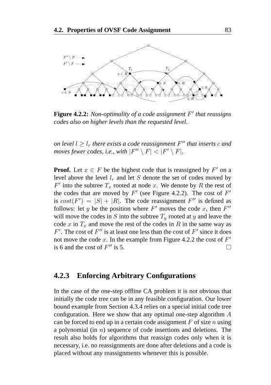
4.2. Properties of OVSF Code Assignment 83
TyTx
x ∈ R
∈ R
c ∈ S∈ S
∈ R
F ′ \ F
F ′′ \ F
∈ S
Figure 4.2.2: Non-optimality of a code assignment F ′ that reassignscodes also on higher levels than the requested level.
on level l ≥ lr there exists a code reassignment F ′′ that inserts c andmoves fewer codes, i.e., with |F ′′ \ F | < |F ′ \ F |.
Proof. Let x ∈ F be the highest code that is reassigned by F ′ on alevel above the level lr and let S denote the set of codes moved byF ′ into the subtree Tx rooted at node x. We denote by R the rest ofthe codes that are moved by F ′ (see Figure 4.2.2). The cost of F ′
is cost(F ′) = |S| + |R|. The code reassignment F ′′ is defined asfollows: let y be the position where F ′ moves the code x, then F ′′
will move the codes in S into the subtree Ty rooted at y and leave thecode x in Tx and move the rest of the codes in R in the same way asF ′. The cost of F ′′ is at least one less than the cost of F ′ since it doesnot move the code x. In the example from Figure 4.2.2 the cost of F ′
is 6 and the cost of F ′′ is 5.
4.2.3 Enforcing Arbitrary Configurations
In the case of the one-step offline CA problem it is not obvious thatinitially the code tree can be in any feasible configuration. Our lowerbound example from Section 4.3.4 relies on a special initial code treeconfiguration. Here we show that any optimal one-step algorithm Acan be forced to end up in a certain code assignment F of size n usinga polynomial (in n) sequence of code insertions and deletions. Theresult also holds for algorithms that reassign codes only when it isnecessary, i.e. no reassignments are done after deletions and a code isplaced without any reassignments whenever this is possible.

84 Chapter 4. OVSF Code Assignment
The idea of the construction is to force the algorithm into a codeassignment with full capacity (the whole bandwidth is assigned) F ′,with F ⊂ F ′, and then to delete the codes that are not present inF . The construction starts with an originally empty code assignmentF0. The following theorem states that algorithm A can be forced toproduce an arbitrary full capacity assignment F ′.
Theorem 4.4 Any one-step optimal algorithm A can be led to an ar-bitrary full capacity assignment F ′ with n′ assigned codes by a re-quest sequence of length m′ < 3n′.
Proof. The construction goes from the top levels towards the leaves:for the current level l we insert codes in all positions that are notblocked by codes on the levels above. Then all codes on level l thatare not in F ′ are deleted and the construction proceeds recursivelyto the lower levels until the assignment F ′ is obtained. The numberof insertions used in this process is bounded from above by the totalnumber of nodes of a binary tree (not necessarily complete) that hasas leaves the code positions in F ′. Since the size of F ′ is n′ we knowthat the number of nodes in such a binary tree is at most 2n′ − 1.The number of deletions is the number of insertions minus the size ofF ′. In conclusion the total number of insertions and deletions usedto force algorithm A to produce the code assignment F ′ is boundedfrom above by 3n′.
Now for arbitrary configurations we can state the following corol-lary.
Corollary 4.5 Any one-step optimal algorithm A can be forced toproduce a code assignment F of size n in a code tree of height h byusing m < 4n · h code insertions and deletions.
Proof. From Theorem 4.4 we know that algorithm A can be forced toproduce a full capacity assignment F ′ of size n′ using a sequence ofat most 3n′ code insertions and deletions. We are interested in the fullcapacity assignment F ′ that is a superset of F and has the minimalnumber of additional codes that are not in F . Each code in F causesat most h additional codes to fill the gaps in F to get the full capacityassignment F ′. This means the size of F ′ is bounded from aboveby n · h and can be constructed using at most 3n · h insertions and

4.2. Properties of OVSF Code Assignment 85
deletions. From F ′ to get to F we have to delete at most n · h codes.Altogether we need at most 4n · h code insertions and deletions.

86 Chapter 4. OVSF Code Assignment
4.3 One-Step Offline CA
4.3.1 Non-Optimality of Greedy Algorithms
The one-step offline CA problem was first presented in [64] and a cer-tain greedy algorithm, called DCA, was claimed to solve the problemoptimally. Here we analyze a more general class of greedy algorithms(that includes as a special case the algorithm DCA) for the one-stepoffline CA problem and prove their non-optimality.
A straight-forward greedy approach is to select for a code inser-tion a subtree with minimum cost that is not blocked by a code abovethe requested level, according to some cost function. All codes in theselected subtree must then be reassigned. So in every step a top-downgreedy algorithm chooses the maximum bandwidth code that has tobe reassigned, places it at the root of a minimum cost subtree, takesout the codes in that subtree and proceeds recursively. The DCA-algorithm in [64] works in this way. In [64] the authors propose dif-ferent cost functions, among which the “topology search” cost func-tion is claimed to solve the one-step offline CA optimally. Here weshow the following theorem:
Theorem 4.6 Any top-down greedy algorithm Atdg depending onlyon the current assignment of the considered subtree is not optimal.
As all proposed cost functions in [64] depend only on the currentassignment of the considered subtree, this theorem implies the non-optimality of the DCA-algorithm.
Proof. Our construction considers the subtrees in Figure 4.3.1 andthe assignment of a new code to the root of the tree T0. The rest ofthe subtrees that are not shown are supposed to be fully assigned withcodes on the leaf level, so that no optimal algorithm would considerto move codes into those subtrees. The tree T0 has a code with band-width 2k on level l and depending on the cost function has or doesnot have a code with bandwidth k on level l − 1. The subtree T1
contains k − 1 codes at leaf level and the rest of the subtree is empty.The subtrees T2 and T3 contain k codes at leaf level interleaved withk free leaves. From Corollary 4.5 we know that any optimal one stepalgorithm can be forced to produce such an assignment. This originalassignment rules out all cost functions that do not put the initial codeat the root of T0. We are left with two cases:

4.3. One-Step Offline CA 87
2kk
T0
T1
...
T2
...
T3
k-1,k+1
OPT
DCA
1
11
1
k-1k/2
k
01
l-1l
level
Figure 4.3.1: Example for the proof of Theorem 4.6.
case 1: The cost function evaluates T2 and T3 as cheaper than T1.In this case we let the subtree T0 contain only the code withbandwidth 2k. Algorithm Atdg reassigns the code with band-width 2k to the root of the subtree T2 or T3, which causes onemore reassignment than assigning it to the root of T1, hence thealgorithm fails to produce the optimal solution.
case 2: The cost function evaluates T1 as cheaper than T2 and T3. Inthis case we let the subtree T0 have both codes. Atdg movesthe code with bandwidth 2k to the root of T1 and the code withbandwidth k into the tree T2 or T3, see solid lines in Figure4.3.1. The number of reassigned codes is 3k/2 + 2. But theminimum number of reassignments is k + 3, achieved whenthe code with bandwidth k is moved in the empty part of T1
and the code with bandwidth 2k is moved to the root of T2 orT3, see dashed lines in Figure 4.3.1.
4.3.2 NP-Hardness
In this part we prove that the decision variant of the one-step offlineCA problem is NP-complete. The decision variant of the one-stepoffline CA problem asks whether a new code request can be satis-fied with at most cmax reassignments. The problem is obviously inNP since one can guess an optimal solution and it can be checked

88 Chapter 4. OVSF Code Assignment
q
triplettrees
receivertrees fill trees
· · · · · ·token tree
code requestfor this level
Figure 4.3.2: Initial code tree configuration for the reduction from a3DM instance.
in polynomial time if it is feasible and if it has cost less than cmax.We prove the NP-completeness by using a reduction from the three-dimensional matching problem (3DM), known to be NP-complete,that is defined in [42] as follows:
Problem 4.7 (3DM) Given a set M ⊆ X × Y × Z, where X,Yand Z are disjoint sets having the same number q of elements. DoesM contain a matching, i.e., a subset M ′ ⊆ M such that |M ′| = qand no two elements of M ′ agree in any coordinate?
To transform an 3DM instance into a code assignment instance wefirst index the elements of the ground sets X,Y,Z from 1 to q. Nextwe introduce the indicator vector of a triplet (xi, yj , zk) as a zero-onevector of length 3q that is all zero except at the indices i, q + j and2q+k. The idea of the reduction is to use the indicator vectors insteadof the triplets and to observe that the problem 3DM is equivalent tofinding a subset of q indicator vectors that represent triplets in M suchthat their sum is the all-one vector.
A 3DM instance is transformed into an initial feasible assignmentusing the code tree from Figure 4.3.2. The initial assignment consistsof a token tree having q codes that are forced by a new code assign-ment into the root of this tree to move into the roots of the triplet trees.The codes from the triplet trees are reassigned into the receiver trees.The fill trees complete the code tree. The choice of the q triplet treeswhere the codes from the token tree are moved reflects the choice ofthe corresponding triplets of a matching. The codes from the triplettrees find place in the receiver trees without additional reassignmentsif and only if their triplet trees represent a three-dimensional match-ing.

4.3. One-Step Offline CA 89
(a) The zero tree. (b) The one-tree.
(c) A layer, consisting of a one-tree and itssibling.
0000
0000
1
(d) Stacking lay-ers.
Figure 4.3.3: Encoding of zero and one.
The codes in the token tree are positioned arbitrarily on levellstart. The triplet trees are constructed from the indicator vectors andhave their roots on the same level lstart. For each of the 3q positionsof the indicator vector a triplet tree has four levels – together calleda layer – that encode either zero or one. We show this encoding inFigure 4.3.3 (a) and (b). Even though the zero and one encoding sub-trees in a certain layer contain the same number of codes and occupythe same bandwidth they are still different. Figures 4.3.3 (c) and (d)show how layers are stacked using sibling trees.
The receiver trees are supposed to receive all codes in the chosentriplet trees. These codes fit exactly in the free positions, if and onlyif the chosen triplets form a 3DM, i.e. if their indicator vectors sumup to the all-one vector. The fill trees are trees that are completely fulland have one more code than the receiver trees. They fill up the levellstart in the sibling-tree of the token tree.
An interesting question is whether this transformation from 3DMto the one-step offline CA can be done in polynomial time. This de-pends on the input encoding of our problem. To us, two encodingsseem natural:
• a zero-one vector that specifies for every node of the tree ifthere is a code or not,
• a sparse representation of the tree, consisting only of the posi-

90 Chapter 4. OVSF Code Assignment
tions of the assigned codes.
The transformation cannot be done in polynomial time for the firstinput encoding, because then the generated tree would have exponen-tially many leaves (exponential in q). For the second input encodingthe transformation is polynomial, because the total number of gen-erated codes is polynomial in q, which is polynomial in the inputsize of 3DM. Another indication that we should rather not expect anNP-completeness proof for the first input encoding, is the exact al-gorithm from Section 4.3.3 that would suggest nO(log n)-algorithmsfor all problems in NP .
We now state the crucial property of the construction in a lemma:
Lemma 4.8 Let M be an input for 3DM and φ the transformationdescribed above. Then M ∈ 3DM if and only if φ(M) can be donewith α = 21q2 + 2q + 1 reassignments.
The proof of Lemma 4.8 is based on counting arguments that be-come obvious from examining the code tree configuration used forthe reduction. It can be found in [28] and will appear also in M.Nunkesser’s thesis. We conclude this section with the following the-orem:
Theorem 4.9 The decision variant of the one-step offline CA is NP-complete for an input given by a list of positions of the assigned codesand the code insertion level.
4.3.3 Exact nO(h) Algorithm
In this section we solve the one-step offline CA problem optimallyusing a dynamic programming approach. The key idea of the result-ing algorithm is to store the right information in the nodes of the treeand to build it up in a bottom-up fashion.
We define the signature of a subtree Tv with root v to be anl(v) + 1-dimensional vector sv = (sv
0, . . . , svl(v)), in which sv
i is thenumber of codes in Tv on level i. An example with code assignmentand node signatures is shown in Figure 4.3.4. A signature s is feasibleif there exists a subtree Tv with a code assignment that has signatures. For every node v of the code tree we build a table in which all pos-sible feasible signatures of an arbitrary tree of height l(v) are stored

4.3. One-Step Offline CA 91
(2, 1, 1, 0)
(2, 1, 0) (0, 0, 1)
(0, 1) (2, 0) (0, 0) (0, 0)
(0) (0) (1) (1) (0) (0) (0) (0)
Figure 4.3.4: Node signatures.
together with their cost for Tv . The cost of a possible signature s forTv (usually s is different from the original signature sv of T v) is de-fined as the minimum number of codes in Tv that have to move awayfrom their old position in order to attain a tree T ′
v with signature s.To attain T ′
v it might be necessary to move codes into Tv from othersubtrees but we do not count these movements in the cost of s for Tv .
Given a code tree T with all these tables computed, one can com-pute the cost of any single code insertion on level l from the table atthe root node r: Let sr = (sr
0, . . . , srh) be the signature of the whole
code tree before insertion, then the cost of the insertion is the cost ofthe signature (sr
0, . . . , srl + 1, . . . , sr
h) in this table plus one (for theoriginal assignment).
The computation of the tables starts at the leaf level, where thecost of the one-dimensional signatures is trivially defined. At anynode v of level l(v) the cost c(v, s) of signature s for Tv is computedfrom the cost incurred in the node’s left subtree Tl plus the cost in-curred in its right subtree Tr plus the cost at v. The costs c(l, s′) andc(r, s′′) in the subtrees come from two feasible signatures with theproperty s = (s′0 + s′′0 , . . . , s′l(v)−1 + s′′l(v)−1, sl(v)). We use the no-tation s = (s′ + s′′, sl(v)) to represent the composition of signature susing the lower level signatures s′ and s′′. Any pair s′, s′′ of such sig-natures corresponds to a possible configuration after the code inser-tion. The best pair for node v gives c(v, s). Let sv = (sv
0, . . . , svl(v))
be the signature of Tv and s′, s′′ are chosen such that s = (s′+s′′, 0),

92 Chapter 4. OVSF Code Assignment
then the following holds:
c(v, s) =
⎧⎪⎨⎪⎩c(l, (0, . . . , 0)) + c(r, (0, . . . , 0)), sl(v) = 1mins′,s′′c(l, s′) + c(r, s′′), sl(v) = 0, sv
l(v) = 01, sl(v) = 0, sv
l(v) = 1.
The costs of all signatures s for v can be calculated simultane-ously by combining the two tables in the left and right children of v.For the running time observe that the number of feasible signatures isbounded by (n + 1)h because there cannot be more than n codes onany level. The time to combine two tables is O(n2h), thus the totalrunning time is bounded by O(2h · n2h).
Theorem 4.10 The one-step offline CA can be optimally solved intime O(2h · n2h) and space O(h · nh).
4.3.4 h-Approximation Algorithm
In this section we analyze a natural greedy algorithm for the one-stepoffline CA problem. The algorithm assigns the new code c0 to theroot of a subtree Tg at level l(c0) that contains the minimum numberof assigned codes between all subtrees available at this level. Bythe availability of a subtree at level l we mean that it is not blockedfrom above and the root of the subtree is free. We are interested onlyin these trees because we know from Lemma 4.3 that no codes areassigned into subtrees that are blocked by levels above the level of thecode. The codes from Tg are reassigned in a top-down fashion startingwith the highest level codes and continuing recursively with the lowerlevels until no more codes have to be reassigned. The pseudocode ofthe algorithm Agreedy is presented in Algorithm 4.11, where Γ(T t
g)represents the assigned codes in the subtree Tg at time t.
At every iteration step t algorithm Agreedy keeps track of the setCt of codes that have to be reassigned into the current tree T t. Ini-tially, C0 = c0 and T 0 = T .
In [64] a similar algorithm was presented as a heuristic for theone-step offline CA but without mentioning theoretical bounds on itsapproximation ratio. We prove that Agreedy has approximation ratioh and this bound is asymptotically tight.

4.3. One-Step Offline CA 93
Algorithm 4.11 Greedy algorithm Agreedy
begin1: C0 ← c0; T 0 ← T2: t ← 03: while Ct = ∅ do4: ct ← element with highest level in Ct
5: g ← the root of a subtree T tg of level l(ct) with
the fewest codes in it and no code on or above its root6: /* assign ct to position g */7: T t+1 ← (T t \ Γ(T t
g)) ∪ g8: Ct+1 ← (Ct ∪ Γ(T t
g)) \ ct9: t ← t + 1
10: end whileend Agreedy
First we show that Agreedy can be forced to use Ω(h) · OPTreassignments (see Figure 4.3.5), where OPT refers to the numberof reassignments an optimal algorithm needs. A new code c0 is as-signed by Agreedy to the root of Tg (which contains the least numberof codes). The two codes on level l − 1 from Tg are reassigned asshown in Figure 4.3.5, one code can be reassigned into Topt and theother one goes recursively into T1. In total, Agreedy does 2 · l + 1reassignments while the optimal algorithm assigns c0 into the root ofTopt and reassigns the three codes from the leaf level into the treesT1, T2, T3, requiring only 4 reassignments. Obviously, for this exam-ple Agreedy is not better than (2l+1)/4 times the optimal. In generall can be Ω(h).
To show the upper bound we compare the code movements of thegreedy algorithm Agreedy to the code movements of an optimal algo-rithm Aopt. The optimal algorithm Aopt assigns the new code c0 intothe root of the subtree Tx0 and the codes from this subtree are movedto other subtrees. We call the subtrees in the root of which Aopt re-assigns the codes opt-trees and we denote the set of these subtrees byTopt. By V (Topt) we denote the set of nodes in Topt. The opt-arcs arethe pairs (u, v) of source-destination nodes describing the code move-ments of Aopt. Figure 4.3.6 shows an example instance together withthe code movements done by Agreedy and an optimal algorithm Aopt.

94 Chapter 4. OVSF Code Assignment
l l−
1
l−
2
l−
3
l−
4
0
Tg
T1
T2
T3
Topt
c 0
...
Agreedy
Aopt
Figure 4.3.5: Lower bound example for Agreedy .

4.3. One-Step Offline CA 95
gc0
x0
an opt-arc greedy assignment
Figure 4.3.6: Greedy against optimal code reassignments, an exam-ple.
Our proof works as follows: we show that in every step t of al-gorithm Agreedy there is the possibility to assign the codes in Ct topositions inside the opt-trees. We express this possibility with a codemapping φt : Ct → V (Topt). The main property of the greedy algo-rithm is that in every step t it is possible to complete the assignmentof the codes in Ct by using φt to move them into the opt-trees andthe opt-arcs to move the codes from the opt-trees. The proof of The-orem 4.16 shows that this property ensures that Agreedy is not worsethan O(h) · OPT .
To make the proof technically precise we introduce the followingdefinitions. In the process of the algorithm some opt-arcs have to bechanged in order to ensure the existence of φt. These changed opt-arcs are represented by the αt-arcs.
Definition 4.12 Let Topt be the set of the opt-trees for a code inser-tion c0 and let T t (together with its code assignment F t) be the codetree after t steps of the algorithm Agreedy . An α-mapping at time tis a mapping αt : Mαt
→ V (Topt) for some Mαt⊆ F t, such that
∀v ∈ Mαt: l(v) = l(α(v)) and αt(Mαt
) ∪ (F t \ Mαt) is a code
assignment.
The set αt(Mαt) ∪ (F t \ Mαt
) represents the resulting code assign-ment after the reassignment of the codes Mαt
⊆ F t by αt.
Definition 4.13 Let T t be a code tree, x, y be positions in T t andαt be an α-mapping. We say that y depends on x in T t and αt, ifthere is a path from x to y using only tree-edges from a parent to achild and αt-arcs. By dept(x) we denote the set of all positions y thatdepend on x in T t and αt. We say that an αt arc (u, v) depends on xif u ∈ dept(x).

96 Chapter 4. OVSF Code Assignment
x
αt
αt
αtαt
αt
Figure 4.3.7: Dependency set of x (grayed subtrees).
In Figure 4.3.7 we show the dependency set dept(x) of a code x.
Definition 4.14 At time t a pair (φt, αt) of a code mapping φt :Ct → V (Topt) and an α-mapping αt is called an independent map-ping for T t, if the following properties hold:
1. ∀c ∈ Ct the levels of φt(c) and c are the same (i.e. l(c) =l(φt(c)).
2. ∀c ∈ Ct there is no code in T t at or above the roots of the treesin dept(φt(c)).
3. the code movements realized by φt and αt (i.e. the set φt(Ct)∪αt(Mαt
) ∪ (F t \ Mαt)) form a code assignment.
4. all nodes in the domain Mαtof αt are in dept(φt(Ct)) (i.e., no
unnecessary arcs are in αt).
Here for φt and αt we used their representation as an arc which isequivalent to the function representation. We abused the notation forthe dependency set of a node and we extended it to the dependencyset of a node set: dept(φt(Ct)) stands for the set
⋃c∈Ct
dept(φt(c)).From these definitions we can draw the following observations: Fortwo independent positions u, v ∈ T and for an independent mapping(φt, αt) we have dept(u) ∩ dept(v) = ∅, i.e. the αt-arcs of indepen-dent positions point into disjoint subtrees. If we have an independentmapping (φt, αt) for T t, then dept(φt(Ct)) is contained in opt-treesand every node in dept(φt(Ct)) can be reached through exactly one

4.3. One-Step Offline CA 97
path from Ct (using one φt-arc and an arbitrary sequence of tree-arcs, which always go from parent to child, and αt-arcs from a codec ∈ Γ(T t) to αt(c)).
We now state an important invariant of the greedy algorithm.
Lemma 4.15 For every set Ct and code tree T t in algorithm Agreedy
there exists an independent mapping (φt, αt).
Proof. The proof is done by induction on t and shows how to con-struct an independent mapping (φt+1, αt+1) from (φt, αt) by caseanalysis. The detailed proof can be found in [28] and will be includedin the thesis of M. Mihalak. Lemma 4.15 actually applies to all algorithms that work level-wisetop-down and choose a subtree T t
g for each code ct ∈ Ct arbitrarilywith the condition that there is no code on or above the node g.
The cost of the optimal algorithm can be expressed in two ways:(a) it is equal to the number of assigned codes in the opt-trees plusone; (b) it is equal to the number of opt-trees. In the following theo-rem we state the approximation ratio of the greedy algorithm.
Theorem 4.16 The algorithm Agreedy has approximation ratio h.
Proof. Since algorithm Agreedy works level-wise top-down all wehave to show is that when it reassigns the codes on level l it incurs acost of at most OPT . Consider the step t of Agreedy when the firstcode on level l from Ct has to be assigned and let there be ql codesof level l in Ct. We know from Lemma 4.3 and the fact that Agreedy
works level-wise top-down that in later steps there will be no othercodes of level l added to Ct+i. The greedy algorithm assigns all ql
codes of level l into subtrees of T t having the minimum number ofassigned codes. From Lemma 4.15 we know that there is an indepen-dent mapping (φt, αt), and hence φt maps the level l codes from Ct
into different independent positions in the opt-trees. Therefore, thecost of the φt mapping restricted to the level l codes from Ct is upperbounded by OPT (total cost of Aopt) and is at least the cost incurredby the greedy assignment of the ql codes on level l from Ct. Hence,on every level the greedy algorithm Agreedy incurs a cost (number ofcodes that are moved away from their position in the tree) that is atmost Aopt’s total cost.

98 Chapter 4. OVSF Code Assignment
ins : N at 0 del : N/2 at 0 ins : 1 at h − 1
A
Aopt
costA
costopt
N
N
0
0
N/4 + 1
1
del : N/4 at 0
. . .
. . .
Figure 4.4.1: Lower bound for the online CA problem.
4.4 Online CA
A practically more relevant version of the code assignment problem iswhere several code insertions and deletions have to be satisfied in anonline fashion. In this section we give a lower bound on the competi-tive ratio of any deterministic online algorithm, analyze several onlinestrategies and present a resource augmented algorithm with constantcompetitive ratio.
Theorem 4.17 No deterministic algorithm A for the online CA prob-lem can be better than 1.5-competitive.
Proof. Let A be any deterministic algorithm for the problem. First theadversary asks for N leaf insertions. The adversary Aopt makes theinsertions in such a way that later on it needs no additional reassign-ments. In the next step the adversary deletes N/2 codes (every sec-ond from the assignment produced by A) to get the situation in Figure4.4.1. Then a code request on level h−1 causes algorithm A to moveN/4 codes. We can proceed with the left subtree of fully assigned leaflevel codes recursively and repeat this process h−1 times. Thus, Aopt
needs N + h − 1 code assignments. Algorithm A needs N + T (N)code assignments, where T (N) = 1+N/4+T (N/2) and T (2) = 0.After reducing the recursive formula we get the following canonicalform: T (N) = h − 1 + N
2 (1 − 2/N). For costA ≤ c · costOPT we
must have c ≥ 3N/2+h−2N+h−1 −→N→∞ 3/2.

4.4. Online CA 99
4.4.1 Compact Representation Algorithm
The compact representation online strategy maintains the codes in thecode tree T sorted by level from left to right (higher level codes arealways to the right of lower level ones) and compact to the left on thesame level. For a given node/code v ∈ T we denote by l(v) its leveland by w(v) its prefix free path encoding (see Section 4.2). We usethe lexicographic ordering when comparing two nodes given by theirpath encoding. With U we denote the set of unblocked nodes of thetree. The compact representation algorithm maintains the followinginvariants:
Invariant 4.18 ∀ codes u, v ∈ F : l(u) < l(v) =⇒ w(u) < w(v).
Invariant 4.19 ∀ nodes u, v ∈ T : l(u) ≤ l(v)∧u ∈ F ∧v ∈ U =⇒w(u) < w(v).
In what follows we show that this algorithm is not worse thanO(h) times the optimum offline algorithm that knows the sequenceof requests in advance. We also show an example for which the al-gorithm is not asymptotically better than this bound, and hence it isO(h)-competitive.
Theorem 4.20 Algorithm Acompact satisfying the Invariants 4.18and 4.19 performs at most h code reassignments per insertion anddeletion.
Proof. When a request for inserting a code on level l is processedby the algorithm it can happen that there is no free space in the com-pact space allocated for this level. In this case a code from the righthand side neighboring level is moved to make space for the new codeand is recursively inserted on its own level. In the worst case thealgorithm has to reassign one code per level to satisfy the insertionrequest. When a code deletion request on level l is processed by thealgorithm it might happen that the Invariant 4.19 on the levels aboveis violated. Hence, on these levels a code has to be moved from rightto left to fill in the gap produced by the deletion. In the worst casethis can also involve one reassignment per level. Since the numberof levels occupied with codes is bounded from above by h the com-pact representation algorithm does at most h reassignments per codeinsertion/deletion request.

100 Chapter 4. OVSF Code Assignment
Figure 4.4.2: Code assignments for levels 0, 0, 1, 2, 3, 4, . . . , h − 1and four consecutive operations: 1. DELETE(h-1), 2. INSERT(0),3. DELETE(0), 4. INSERT(h-1).
Corollary 4.21 Algorithm Acompact satisfying invariants (4.18) and(4.19) is O(h)-competitive.
Proof. In the sequence σ = σ1, . . . , σm the number of deletions dmust be smaller or equal to the number i of insertions, which impliesd ≤ m/2. The cost of any optimal algorithm is then at least i ≥ m/2.On the other hand, Acompact incurs a cost of at most m · h, whichimplies that it is O(h)-competitive.
Theorem 4.22 Any algorithm AI satisfying invariant (4.18) is Ω(h)-competitive.
Proof. For the sequence of code insertions on levels 0, 0, 1, 2, 3, 4,. . . , h− 1 there is a unique code assignment that satisfies the invariant(4.18), see Figure 4.4.2. Now if the adversary requests the deletion ofthe code at level h−1 and insertion of a code on level 0 then AI has tomove every code on level l ≥ 1 to the right to create space for the codeassignment on level 0 and maintain the invariant (4.18). This takesh−1 code reassignments. Then the adversary requests the deletion ofthe third code on level zero and an insertion on level h− 1. Again, tomaintain the invariant (4.18), AI has to move every code on level l ≥1 to the left. This takes again h − 1 code reassignments. An optimalalgorithm can handle these four requests with two assignments, sinceit can assign the third code on level zero in the right subtree, whereAI assigns the code on level h−1. After repeating these four requestsk times, the total cost of the algorithm AI becomes costI = h + 1 +k · 2(h − 1), whereas Aopt has costOPT = h + 1 + k · 2. When kgoes to infinity, the ratio costA/costOPT becomes Ω(h).

4.4. Online CA 101
Figure 4.4.3: Requests that a greedy strategy cannot handle effi-ciently.
4.4.2 Greedy Online Strategies
An optimal deterministic algorithm Ag for the one-step offline CAproblem can be used as a greedy online strategy. As an optimal algo-rithm breaks ties in an unspecified way, the online-strategy can varyfor different optimal one-step offline algorithms.
Theorem 4.23 Any deterministic greedy online-strategy, i.e. a strat-egy that minimizes the number of reassignments for every insertion,is Ω(h) competitive.
Proof. Assume that Ag is a fixed, greedy online-strategy. First theadversary asks for N/2 code insertions on level 1. As Ag is de-terministic the adversary can now delete every second level-1 code,and ask for inserting N/2 level-0 codes. This leads to the assign-ment shown in Figure 4.4.3. Next the adversary deletes two codes atlevel l = 1 (as Ag is deterministic it is clear which codes to delete)and immediately asks for a code insertion on level l + 1. As it is one-step optimal (and up to symmetry unique) the algorithm Ag reassignstwo codes as shown in the figure. The optimal adversary arrangesthe level-1 codes in a way that it does not need any additional reas-signments. The adversary repeats this sequence along level 1 in thefirst round from left to right, then on level 2 in a second round, andcontinues towards the root. Altogether the greedy algorithm movesN/4 codes in the first round and assigns N/23 codes. In general, inevery round i the greedy strategy reassigns N/4 level-0 codes andassigns N/2i+2 level-i codes. Altogether the greedy strategy needsO(N)+ (N/4)Ω(h) = Ω(N ·h) reassignments, whereas the optimalstrategy needs only O(N) assignments.

102 Chapter 4. OVSF Code Assignment
Figure 4.4.4: Reassignment of one code reduces the number ofblocked codes from 3 to 2.
4.4.3 Minimizing the Number of Blocked Codes
The code assignment strategy that keeps the number of blocked codesminimal was mentioned and tested with simulations in [71]. Howeverno theoretical analysis about the competitiveness of the algorithm waspresented there. Here we give a precise, formal description of thealgorithm and analyze its competitiveness.
The algorithm satisfies the following invariant after every codeinsertion or deletion request (with the precondition that the invariantholds also initially):
Invariant 4.24 The number of blocked codes in T is minimum.
Figure 4.4.4 shows an initial code assignment that does not satisfythe Invariant 4.24. In this example the invariant can be established bymoving one code.
We prove that this algorithm is equivalent to the algorithm thatminimizes the number of gap trees on every level.
Definition 4.25 A gap tree is a maximal subtree of unblocked codes.The level of its root is the level of the gap tree. The vector q =(q0, . . . , qh) is the gap vector of the tree T , where qi specifies thenumber of gap trees on level i.
Figure 4.4.5 highlights the gap trees for an example code assignment.The implication of Invariant 4.24 is that there can be at most one gaptree on every level.
Lemma 4.26 Let F be a code assignment in the code tree T . Then Fblocks a minimum number of codes in T if and only if T has at mostone gap tree on every level.

4.4. Online CA 103
gap treesq = (1, 2, 1, 0, 0)
Figure 4.4.5: Gap trees and gap vector of a code assignment.
Proof. First we prove that it is necessary to have at most one gap treeon every level to minimize the number of blocked codes. If there aretwo gap trees Tu, Tv on a level l then by moving the codes from thesibling tree T ′
u of Tu into the gap tree Tv we create a gap tree at levell + 1 rooted at the parent of u and hence we reduce the number ofblocked codes by one. This shows that having at most one gap treeper level is a necessary condition to minimize the number of blockedcodes.
Next we prove the sufficiency of the condition. Suppose that Fleaves at most one gap tree on every level of T . The free bandwidthcapacity of T can be expressed as
cap =h∑
i=0
qi · 2i.
Since qi ∈ 0, 1, the gap vector is the binary representation of thenumber cap. Therefore the gap vector q is the same unique vector forall code assignments having at most one gap tree at every level andserving the same requests as F . The gap vector determines also thenumber of blocked codes:
# blocked codes =(2h+1 − 1) −h∑
i=0
qi(2i+1 − 1).

104 Chapter 4. OVSF Code Assignment
Algorithm 4.27 Algorithm, Agap(op, l, c)in: op - requested operation (insert/delete); l - level of the insertion;c - code to be deleted;parameter: T - code tree; q - gap vector of T ; h - height of Tbegin
1: if op = insert then2: assign new code into the smallest gap tree of level ≥ l3: else4: delete(c, T )5: q = gapvector(T )6: for (i = 0; i ≤ h; inc(i)) do7: if qi > 1 then8: reduce number of gap trees at level i by filling in one of
the gap trees with codes from the sibling of the other gaptree
9: q = gapvector(T )10: end if11: end for12: end ifend Agap
This shows that any code assignment having at most one gap tree perlevel and serving the same requests as F has the same number ofblocked codes as F .
In Algorithm 4.27 we show the pseudo code of Agap.
Lemma 4.28 The algorithm Agap always has a gap tree of sufficientheight to assign a code on level l and satisfies the Invariant 4.24.
Proof. First we show that the algorithm Agap satisfies the Invari-ant 4.24 by showing that the tree T after the algorithm returns hasat most one gap tree on every level. Consider an insertion into thesmallest gap tree of level l′ where the code fits. New gap trees canoccur only on levels j, l ≤ j < l′ and only within the gap tree onlevel l′. At most one new gap tree can occur on every level. Supposethat after creating a gap tree on level j, we have more than one gaptrees on this level. Then, since j < l′, we would assign the code intothis smaller gap tree, a contradiction (Figure 4.4.6). Therefore, after

4.4. Online CA 105
j j
l’
l...
Figure 4.4.6: Two gap trees on a lower level than l′ violate the mini-mality of the chosen gap tree.
an insertion there is at most one gap tree on every level.
After a code deletion the nodes of the subtree of that code becomeunblocked, i.e., they belong to some gap tree. At most one new gaptree can occur after a delete operation (and some gap trees may disap-pear). Thus, when the newly created gap tree is the second one on thelevel, we fill the gap trees and then we iteratively handle the newlycreated gap tree on a higher level. In this way the gap trees are movedup. Because we cannot have two gap trees on level h − 1, we end upwith a tree with at most one gap tree on each level.
From the precondition of the online CA problem we know thatthere is sufficient capacity to serve the request, i.e. cap ≥ 2l. We alsoknow that cap =
∑i qi2i and because qi ∈ 0, 1 for all i (q is the
unique binary representation of cap), there exists a gap tree on levelj ≥ l.
Algorithm Agap does not need any extra code movements afterinsertions and hence is optimal when only code insertions are con-sidered. However, when deletions are also allowed the algorithm isΩ(h)-competitive.
Theorem 4.29 Algorithm Agap is Ω(h)-competitive.
Proof. The request sequence from the proof of Theorem 4.23 showsthe Ω(h)-competitiveness of algorithm Agap.

106 Chapter 4. OVSF Code Assignment
4.4.4 Resource Augmented Online Algorithm
In this section we present an online-strategy called 2-gap that is al-lowed to use twice the amount of resource the offline adversary is us-ing. Resource augmented online strategies were introduced in 1995by Kalyanasundaram and Pruhs [53] for scheduling problems. Later,in 2000, it was presented as an online analysis technique in [54]. In aresource-augmented competitive analysis one compares the value ofthe solution found by the online algorithm when it is provided withmore resources to the value of the optimal offline adversary using theoriginal resources. In the case of the OVSF online code assignmentproblem the resource is the total assignable bandwidth. The strategy2-gap uses a tree T ′ of bandwidth 2b to accommodate codes whosetotal bandwidth is b. By the nature of the code assignment we cannotadd a smaller amount of additional resource, even though our onlinestrategy needs only 1.5 times the amount of the nominal bandwidth b.Here we prove that 2-gap uses only an amortized constant number ofreassignments per insertion or deletion.
The algorithm 2-gap is similar to the compact representation al-gorithm of Section 4.4.1 (where codes are ordered according to theirlevel, Invariant (4.18)), only that it allows for up to 2 gaps at eachlevel l (instead of only one for aligning), to the right of the assignedcodes on l. For inserting a code at level l the algorithm assigns it inthe leftmost gap on this level. If no such gap exists, the leftmost codeof the next higher level l + 1 is reassigned, creating 2 gaps on level l(one of them is filled immediately by the new code). The algorithmrepeats this procedure towards the root until no more codes have tobe reassigned. An insertion is rejected if the nominal bandwidth bis exceeded. For deleting a code c on level l the rightmost code onlevel l is moved into the place of c, keeping all codes at level l leftof the gaps of l. If this results in 3 consecutive gaps, the rightmostcode on level l + 1 is reassigned, in effect replacing two gaps of lby one of l + 1. The algorithm proceeds towards the root until nolevel has more than two gaps. More precisely, for every level the al-gorithm 2-gap keeps a range of codes (and gaps) that are assignedto this level. In every range there can be at most 2 gaps. If there isno space in the range for a new code or if there are too many gaps,the boundary between two consecutive levels is moved, affecting twoplaces on the lower level and one on the upper level. This notion ofa range is in particular important for levels without codes. The levels

4.4. Online CA 107
close to the root are handled differently, to avoid an excessive spaceusage. The root-code of T ′ has bandwidth 2b and it is never used.The bandwidth b code can only be used if no other code is used. Theb/2 codes are kept compactly to the right. In general there is someunused bandwidth between the highest level l ≤ b/4 codes and theb/2 codes. This unused bandwidth is considered as one gap on level lonly if the nominal capacity b would still allow a code on l, otherwiseit is not counted as a gap. For all other levels (≤ b/8 codes) we de-fine a potential-function that is equal to the number of levels withoutgaps together with the number of levels having 2 gaps. The reasonwhy we count these levels is because they can produce additional re-assignments in case of an insertion or deletion. With this potentialfunction it is sufficient to charge two reassignments to every insertionor deletion, one for placing the code (filling the gap), and one for thepotential function or for moving a b/4-bandwidth code. The initialconfiguration is the empty tree, where the leaf-level has two gaps, andall other levels have precisely one gap (only the close-to-root levelsare as described above).
We have to show that our algorithm manages to host codes aslong as the total bandwidth used does not exceed b. To do this, wecalculate the bandwidth wasted by gaps, which is at most 2( b
8 + b16 +
· · · ) ≤ b/2. Hence the total bandwidth used in T ′ is 3b/2 < 2b.
Theorem 4.30 Let σ be a sequence of m code insertions and dele-tions for a code-tree of height h, such that at no time the bandwidthis exceeded. Then the online-strategy 2-gap using a code-tree ofheight h + 1 performs at most 2m + 1 code reassignments.
Corollary 4.31 The online strategy 2-gap for resource augmentationby a factor of 2 is 4-competitive.
Proof. Any sequence of m operations contains at least m/2 insertoperations. Hence the optimal offline solution needs at least m/2 as-signments, and the above resource augmented online-algorithm usesat most 2m + 1 reassignments, leading to a competitive ratio of 4.
This approach might prove to be useful in practice, particularly ifthe code insertions only use half the available bandwidth.

108 Chapter 4. OVSF Code Assignment
4.5 Discussions and Open Problems
In this chapter we brought an algorithmically interesting problemfrom the mobile telecommunications field closer to the theoreticalcomputer science community. We analyzed several versions of theproblem, but our analysis does not close the OVSF code assignmentproblem. Some interesting open problems remain unanswered:
• Is there a constant approximation algorithm for the one-stepoffline CA problem?
• Can the gap between the lower bound of 1.5 and the upperbound of O(h) for the competitive ratio of the online CA beclosed?
Our paper [29] on OVSF code assignment published in 2004 raisedtwo other open questions:
• Is there an instance where the optimal general offline algorithmhas to reassign more than an amortized constant number ofcodes per insertion or deletion?
• What is the complexity of the general offline CA problem?
Since then these two questions were analyzed in [78] and lead to thefollowing results: the general offline CA problem is NP-completeand there exist instances of code trees for which any optimal offlinegreedy algorithm needs to reassign more than one code per an inser-tion/deletion request. Whether there are instances where more than anamortized constant number of reassignments are necessary remainsstill open.

Chapter 5
Joint Base StationScheduling
5.1 Introduction
We consider different combinatorial aspects of problems arising in thecontext of load balancing in time division networks. These problemsturn out to be related to interval scheduling problems and intervalgraphs.
The general setting is that mobile phone users are served by a setof base stations. For our considerations the user is the mobile device.In each time slot (round) of the time division multiplexing each basestation serves at most one user. Traditionally, each user is assignedto a single base station that serves the user until it leaves the cell ofthe base station or until its demand is satisfied. The amount of datathat a user receives depends on the strength of the signal it receivesfrom its assigned base station and on the interference, i.e. all signalpower it receives from other base stations. In [21], Das et al. proposea novel approach. In their approach clusters of base stations jointlydecide which users to be served in which round in order to increasenetwork performance. Intuitively, if in each round neighboring basestations try to serve pairs of users such that the mutual interferenceis low, this approach increases the throughput. We turn this approachinto a discrete scheduling problem in one and two dimensions (see
109
110 Chapter 5. Joint Base Station Scheduling
Figure 5.1.1), the Joint Base Station Scheduling (JBS) problem.
In one dimension (see Figure 5.1.1(a)) we are given a set of nusers as points u1, . . . , un on a line and we are given positionsb1, . . . , bm of m base stations. Note that such a setting could cor-respond to a scenario where the base stations and users are locatedalong a straight road. In our model, when a base station bj servesa user ui, this creates interference for other users in an interval oflength 2|bj − ui| around the midpoint bj . In any round a base stationis allowed to serve a user only if in that round no other base stationhas signal at that user. Hence, in each round each base station canserve at most one user. The goal is to serve all users in as few roundsas possible. In two dimensions users and base stations are representedas points in the plane. When base station bj serves user ui this cre-ates interference in a disk with radius ‖bj − ui‖2 and center bj (seeFigure 5.1.1(c)).
The one-dimensional problem is closely related to interval schedul-ing problems. The particular way how the interference phenomenaappears leads to directed intervals (arrows). For these, we allow theirtails to intersect (intersecting tails correspond to interference that doesnot affect the users at the heads of the arrows). We present results onthis special interval scheduling problem. Similarly, the problem isrelated to interval graphs, except that we have conflict graphs of ar-rows together with the conflict rules defined by the interference (ar-row graphs).
5.1.1 Related Work
Das et al. [21] propose an involved model for load balancing thattakes into account different fading effects and calculates the result-ing signal to noise ratios at the users for different schedules. In eachround only a subset of all base stations is used in order to keep the in-terference low. The decision on which base stations to use is taken bya central authority. The search for this subset is formulated as a (non-trivial) optimization problem that is solved by complete enumerationand that assumes complete knowledge of the channel conditions. Theauthors perform simulations on a hexagonal grid, propose other algo-rithms, and reach the conclusion that the approach has the potentialto increase throughput.
There is a rich literature on interval scheduling and selection prob-
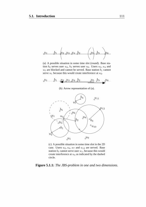
5.1. Introduction 111
b1 b2 b3u1 u2 u3 u4 u5 u6
(a) A possible situation in some time slot (round). Base sta-tion b2 serves user u2, b3 serves user u6. Users u3, u4 andu5 are blocked and cannot be served. Base station b1 cannotserve u1 because this would create interference at u2.
b1 b2 b3u1 u2 u3 u4 u5 u6
(b) Arrow representation of (a).
b1
b2 b3
b4
b5
u2
u4
u7
u12
u1
u3
u5
u6
u8
u9
u10
u11
(c) A possible situation in some time slot in the 2Dcase. Users u2, u4, u7 and u12 are served. Basestation b5 cannot serve user u1, because this wouldcreate interference at u4 as indicated by the dashedcircle.
Figure 5.1.1: The JBS-problem in one and two dimensions.

112 Chapter 5. Joint Base Station Scheduling
lems (see [32, 73] and the references given therein for an overview).Our problem is more similar to a setting with several machines whereone wants to minimize the number of machines required to scheduleall intervals. A version of this problem where intervals have to bescheduled within given time windows is studied in [19]. Inapprox-imability results for the variant with a discrete set of starting timesfor each interval are presented in [18].
5.1.2 Model and Notation
In this section we define the problems of interest. Throughout the pa-per we use standard graph-theoretic terminology, see e.g. [87]. Ourmodel of computation is the real RAM machine. The operands in-volved (positions on the line or in the plane) could be restricted also torational numbers, but to preserve the geometric properties of intervaland disk intersections we use real operands. In the one-dimensionalcase we are given the set B = b1, . . . , bm ⊂ R of base stationpositions and the set U = u1, . . . , un ⊂ R of user positions onthe line in left-to-right order. Conceptually, it is more convenient tothink of the interference region that is caused by some base station bj
serving a user ui as an interference arrow of length 2|bj − ui| withmidpoint bj pointing to the user, as shown in Figure 5.1.1(b). The in-terference arrow for the pair (ui, bj) has its head at ui and its midpointat bj . We denote the set of all arrows resulting from pairs P ⊆ U ×Bby A(P ). If it is clear from the context, we call the interference ar-rows just arrows. If more than one user is scheduled in the sameround then they are allowed to get signal only from their serving basestations, that is, no interference coming from other base stations is al-lowed. Thus, two arrows are compatible if no head is contained in theother arrow; otherwise, we say that they are in conflict. Formally, thehead ui of the arrow for (ui, bk) is contained in the arrow for (uj , bl)if ui is contained in the closed interval [bl−|uj −bl|, bl + |uj −bl|]. Ifwe want to emphasize which user is affected by the interference fromanother transmission, we use the term blocking, i.e., arrow ai blocksarrow aj if aj’s head is contained in ai.
As part of the input we are given only the base station and userpositions. The arrows that show which base station serves whichuser are part of the solution. For each user we have to decide whichbase station serves it. This corresponds to selecting an arrow for the

5.1. Introduction 113
user. At the same time, we have to decide in which round each se-lected arrow is scheduled under the side constraint that all arrows ineach round must be compatible. To distinguish between the differentrounds we have to label the arrows scheduled in these rounds withdifferent labels. The arrows scheduled in the same round should belabeled identically. For labeling the arrows we use colors that repre-sent the rounds.
For the two-dimensional JBS problem we have positions in R2
and interference disks d(bi, uj) with center bi and radius ‖bi − uj‖2
instead of arrows. We denote the set of interference disks for the userbase-station pairs from a set P by D(P ). Two interference disks arein conflict if the user that is served by one disk is contained in theother disk; otherwise, they are compatible. The problems can now bestated as follows:
1D-JBS
Input: User positions U = u1, . . . , un ⊂ R and base station posi-tions B = b1, . . . , bm ⊂ R.
Output: A set P of n user base-station pairs such that each useris in exactly one pair, and a coloring C : A(P ) → N of theset A(P ) of corresponding arrows such that any two arrowsai, aj ∈ A(P ), ai = aj , with C(ai) = C(aj) are compatible.
Objective: Minimize the number of colors used.
2D-JBS
Input: User positions U = u1, . . . , un ⊂ R2 and base stationpositions B = b1, . . . , bm ⊂ R2.
Output: A set P of n user base-station pairs such that each user isin exactly one pair, and a coloring C : D(P) → N of the setD(P) of corresponding disks such that any two disks di, dj ∈D(P), di = dj , with C(di) = C(dj) are compatible.
Objective: Minimize the number of colors used.
The two problems mentioned above are the same except the input in1D-JBS is given on a line and in 2D-JBS is given in the plane. Thearrows can be considered as one-dimensional disks.

114 Chapter 5. Joint Base Station Scheduling
For simplicity we will write ci instead of C(ai) in the rest of thechapter. From the problem definitions above it is clear that both the1D- and the 2D-JBS problems consist of a selection problem and acoloring problem. In the selection problem we want to select onebase station for each user in such a way that the arrows (disks) cor-responding to the resulting set P of user base-station pairs can becolored with as few colors as possible. We call a selection P feasibleif it contains exactly one user base-station pair for each user. Deter-mining the cost of a selection is then the coloring problem. This canalso be viewed as a problem in its own right, where given as input aset of arrows, the task is to schedule them in the minimum numberof rounds. The conflict graph G(A) of a set A of arrows is the graphin which every vertex corresponds to an arrow and there is an edgebetween two vertices if the corresponding arrows are in conflict. Wecall such conflict graphs of arrows arrow graphs. The arrow graphcoloring problem asks for a proper coloring of such a graph. It issimilar in spirit to the coloring of interval graphs. As we will see inSection 5.2.1, the arrow graph coloring problem can be solved in timeO(n log n). We finish this section with a simple lemma that leads toa definition:
Lemma 5.1 For each 1D-JBS instance there is an optimal solutionwith each user being served by the closest base station to its left orright.
Proof. This follows by a simple exchange argument: Take any op-timal solution that does not have this form. Then exchange the ar-row where a user is not served by the closest base station in someround against the arrow from the closest base station on the same side(which must be idle in that round). Shortening an arrow without mov-ing its head can only resolve conflicts. Thus, there is also an optimalsolution with the claimed property.
The two possible arrows by which a user can be served accordingto this lemma are called user arrows. It follows that for a feasibleselection one has to choose one user arrow from each pair of userarrows.

5.1. Introduction 115
5.1.3 Summary of Results
As we already mentioned in Chapter 4 the work presented in thischapter was done in collaboration with T. Erlebach, R. Jacob, M.Mihalak, M. Nunkesser and P. Widmayer. Extended abstracts of theseresults were presented in [30] and [31]. These results will also appearin M. Nunkesser’s and M. Mihalak’s dissertation. We explicitly spec-ify here the parts that were done together with the co-authors and theparts contributed by the author of this thesis. This somewhat forcedpartitioning is not meant to be any clear-cut between parts done bysome of the authors since all the authors were equally involved in thisresearch. However, all authors agreed to present all the results andemphasize more on those results where the corresponding author wasmore involved.
We prove that arrow graphs are perfect and can be colored opti-mally in O(n log n) time. For the one-dimensional JBS problem withevenly spaced base stations we give a polynomial-time dynamic pro-gramming algorithm. For another special case of the one-dimensionalJBS problem, where 3k users must be served by 3 base stations in krounds, we also give a polynomial-time optimal algorithm. From theperfectness of arrow graphs and the existence of a polynomial-timealgorithm for computing maximum weighted cliques in these graphs,we derive a 2-approximation algorithm for JBS based on an LP relax-ation and rounding. In the two-dimensional case deciding whether allusers can be served in one round is doable in polynomial time. Weanalyze an approximation algorithm for a constrained version of the2D-JBS problem, and present lower bounds on the quality of somenatural greedy algorithms for the general two-dimensional JBS prob-lem.
The following results are the contribution from the author of thisdissertation. For the general one-dimensional JBS problem, we showthat for any fixed k the question whether all users can be served in krounds can be solved in nO(k) time. For the 1D-JBS problem we showthat the 2-approximation result can be generalized to a more realisticmodel where the interference region extends beyond the receiver. Weshow that the k-decision version of 2D-JBS (where k ≥ 3) is NP-complete.

116 Chapter 5. Joint Base Station Scheduling
5.2 1D-JBS
As mentioned earlier, solving the 1D-JBS problem requires selectingan arrow for each user and coloring the resulting arrow graph withas few colors as possible. To understand when a selection of arrowsleads to an arrow graph with small chromatic number, we first studythe properties of arrow graphs in relation to existing graph classes.Next we analyze special cases of 1D-JBS that are solvable in polyno-mial time. At the end of this section we present a dynamic programthat solves the decision version of the 1D-JBS problem in time nO(k),where k is the number of rounds, and we show a 2-approximation al-gorithm. The big open problem remains the complexity of the general1D-JBS problem: Is it NP-complete or is it polynomially solvable?
5.2.1 Relation to Other Graph Classes
We will make use of properties of arrow graphs in the design of algo-rithms for 1D-JBS in the following sections. Therefore, let us brieflydiscuss the relationship between arrow graphs and other known graphclasses.1 Exact definitions and further information about the graphclasses mentioned in this section can be found in [12, 74].
Any interval graph is also an arrow graph where all arrows pointin the same direction. Thus, arrow graphs are a superclass of intervalgraphs.
An arrow graph can be represented as the intersection graph of tri-angles on two horizontal lines y = 0 and y = 1: Simply represent anarrow with left endpoint and right endpoint r that points to the right(left) as a triangle with corners (, 0), (r, 0), and (r, 1) (with corners(r, 1), (, 1), and (, 0) respectively). With this representation twotriangles intersect if and only if the corresponding arrows are in con-flict. See Figure 5.2.1 for an example. Intersection graphs of triangleswith endpoints on two parallel lines are known in the literature as PI∗
graphs. They are a subclass of trapezoid graphs, which are the inter-section graphs of trapezoids that have two sides on two fixed parallel
1The connections between arrow graphs and known graph classes such as PI∗graphs, trapezoid graphs, co-comparability graphs, AT-free graphs, and weakly chordalgraphs were observed by E. Kohler, J. Spinrad, R. McConnell, and R. Sritharan at theseminar “Robust and Approximative Algorithms on Particular Graph Classes”, held inDagstuhl Castle during May 24–28, 2004.

5.2. 1D-JBS 117
Figure 5.2.1: An arrow graph (top) and its representation as a PI∗
graph (bottom).
lines. Trapezoid graphs are in turn a subclass of co-comparabilitygraphs, a well-known class of perfect graphs. Therefore, the contain-ment in these known classes of perfect graphs implies arrow graphsare also perfect. Consequently, the size of a maximum clique in anarrow graph equals its chromatic number.
As arrow graphs are a subclass of trapezoid graphs, we can ap-ply known efficient algorithms for trapezoid graphs to arrow graphs.Felsner et al. [34] give algorithms with running-time O(n log n) forchromatic number, weighted independent set, weighted clique, andclique cover in trapezoid graphs with n vertices, provided that thetrapezoid representation is given. The coloring algorithm providedin [34] is very similar to the following greedy coloring algorithm.
We assume for simplicity that the arrows A = a1, . . . , an aregiven in left-to-right order of their left endpoints. This sorting canalso be seen as the first step of the greedy coloring algorithm. The al-gorithm scans the arrows from left to right in this sorted order. In stepi it checks whether there are colors that have already been used andthat can be assigned to ai without creating a conflict. If there are suchcandidate colors, it considers, for each such color c, the rightmostright endpoint rc among the arrows that have been assigned color cso far. To ai is assigned the color c for which rc is rightmost (breakingties arbitrarily). If there is no candidate color, the algorithm assignsa new color to ai. The optimality proof of this algorithm is givenin [30] and it is easy to see that the running time is O(n log n).
We sum up the discussed properties of arrow graphs in the fol-lowing theorem.
Theorem 5.2 Arrow graphs are perfect. In arrow graphs chromatic

118 Chapter 5. Joint Base Station Scheduling
number, weighted independent set, clique cover, and weighted cliquecan be solved in time O(n log n).
One can also show that arrow graphs are AT-free (i.e., do notcontain an asteroidal triple) and weakly chordal. For more detailson these graph classes the interested reader is referred to the text-book [12].
5.2.2 1D-JBS with Evenly Spaced Base Stations
As it usually happens most problems are hard to model and solvewhen all realistic parameters are considered. To gain more under-standing of the structure and the hardness of the problem first simpli-fied models are studied. The simplest and still interesting version ofthe 1D-JBS problem that we can solve in polynomial time is whenbase stations are spaced equidistant. Here we consider the specialcase of the 1D-JBS problem where the base stations are spaced atdistance d from their neighbors. The far-out user on the left (right)side is also not further than distance d from the first (last) base station.We consider the base stations in left-to-right order.
The m base stations partition the line into a set v0, . . . , vm ofintervals. In this special case and from Lemma 5.1 we have the prop-erty that no interference arrow intersects more than two intervals, i.e.the influence from a base station is limited to its direct left and rightneighboring base station. A solution (selection of arrows) is con-sidered non-crossing if there are no two users u and w in the sameinterval such that u is to the left of w, u is served from the right, andw from the left, in two different rounds.
Lemma 5.3 For instances of 1D-JBS with evenly spaced base sta-tions, there is always an optimal solution that is non-crossing.
Proof. Consider an optimal solution that violates the non-crossingproperty. Let u and w be two users such that u and w are in the sameinterval, u is to the left of w, and the optimal solution s serves u withthe right base station br in round t1 using arrow ar and w with the leftbase station bl in round t2 using arrow al; obviously, t1 = t2. We canmodify s such that in round t1 base station br serves w and in t2 basestation bl serves u. The modified solution is feasible because boththe left and the right involved arrows al and ar have become shorter,
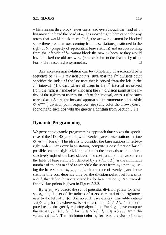
5.2. 1D-JBS 119
which means they block fewer users, and even though the head of al
has moved left and the head of ar has moved right there cannot be anyarrow that would block them. In t1 the arrow ar cannot be blockedsince there are no arrows coming from base stations positioned to theright of br (property of equidistant base stations) and arrows comingfrom the left side of br cannot block the new ar because they wouldhave blocked the old arrow ar (contradiction to the feasibility of s).For t2 the reasoning is symmetric.
Any non-crossing solution can be completely characterized by asequence of m − 1 division points, such that the ith division pointspecifies the index of the last user that is served from the left in theith interval. (The case where all users in the ith interval are servedfrom the right is handled by choosing the ith division point as the in-dex of the rightmost user to the left of the interval, or as 0 if no suchuser exists.) A straight forward approach is to enumerate all possibleO(nm−1) division point sequences (dps) and color the arrows corre-sponding to each dps with the greedy algorithm from Section 5.2.1.
Dynamic Programming
We present a dynamic programming approach that solves the specialcase of the 1D-JBS problem with evenly spaced base stations in timeO(m · n4 log n). The idea is to consider the base stations in left-to-right order. For every base station, compute a cost function for allpossible left and right division points in the intervals to the left re-spectively right of the base station. The cost function that we store inthe table of base station bi, denoted by χi(di−1, di), is the minimumnumber of rounds needed to schedule the users from u1 up to udi
us-ing the base stations b1, b2, . . . , bi. In the case of evenly spaced basestations this cost depends only on the division point positions di−1
and di that define the users served by the base station bi. An examplefor division points is given in Figure 5.2.2.
By Λ(vi) we denote the set of potential division points for inter-val vi, i.e., the set of the indices of users in vi and of the rightmostuser to the left of vi (or 0 if no such user exists). The table entriesχ1(d0, d1) for b1, where d0 is set to zero and d1 ∈ Λ(v1), are com-puted using the greedy coloring algorithm. For i ≥ 1, we computethe values χi+1(di, di+1) for di ∈ Λ(vi), di+1 ∈ Λ(vi+1) from thevalues χi(·, di). The minimum coloring for fixed division points di

120 Chapter 5. Joint Base Station Scheduling
v0 v1
b1 b2 bi−1 bi bi+1 bm
vi−1 vi vm
d0 d1 di−1 di di+1 dm
. . . . . .
Figure 5.2.2: Dynamic programming approach.
and di+1 at base station bi+1 is the maximum between the number ofcolors needed at bi, using the same di and choosing di−1 such thatχi(di−1, di) is minimized, and the coloring ci of the arrows intersect-ing the interval vi. In the case of evenly spaced base stations withno “far out” users this cost ci depends only on the division pointsdi−1, di and di+1 and we denote it by ci(di−1, di, di+1). The col-oring χi(di−1, di) is compatible with the coloring ci(di−1, di, di+1)up to redefinition of colors. The algorithm chooses the best divisionpoint di−1 to get:
χi+1(di, di+1) = mindi−1∈Λ(vi−1)
max χi(di−1, di), ci(di−1, di, di+1)
The running time is dominated by the calculation of the ci values.There are O(m · n3) such values, and each of them can be computedin time O(n log n) using the coloring algorithm. The optimal solu-tion is found by tracing back where the minimum was achieved fromχm(x, n). Here x is chosen among the users of the interval beforethe last base station such that χm(x, n) is minimum. For the trace-back it is necessary to store a pointer to the entry in the previous tablewhere the minimum was achieved in the computation of the χ val-ues. The traceback yields a sequence of division points that definesthe selection of arrows for an optimal schedule. The following the-orem summarizes our result for the 1D-JBS with evenly spaced basestations:
Theorem 5.4 The base station scheduling problem for evenly spacedbase stations without “far out” users can be solved in O(m · n4 log n)time by dynamic programming.
The running time is further bounded by O(m · u4max log umax),
where umax is the maximum number of users in one interval.

5.2. 1D-JBS 121
5.2.3 3k Users, 3 Base Stations in k Rounds
Here we analyze the following special case of the 1D-JBS problem:We are given 3 base stations b1, b2 and b3, and 3k users with k far outusers among them. Far out users are the users to the left of b1 or tothe right of b3 whose interference arrows contain b2. We want to findout whether the users can be served in k rounds or not.
This special setting forces every base station to serve a user inevery round if there is a k-schedule. A far out user has to be servedby its unique neighboring base station. Since the arrows of far outusers contain b2, all users between b1 and b2 are blocked when thefar out users of b1 are served. Hence they have to be served when thefar out users of b3 are served. Based on this observation every roundcontains one of the following types of arrow triplets:
Type 1: b3 serves a far out user, b2 serves a user between b1 and b2,and b1 serves a user that is not a far out user.
Type 2: b1 serves a far out user, b2 serves a user between b2 and b3,and b3 serves a user that is not a far out user.
For every user, it is uniquely determined whether it will be served ina round of Type 1 or Type 2.
We can schedule the users in the following way. Let k1 and k3 bethe number of far out users of b1 and b3 respectively with k = k1+k3.First, we serve the far out users of b3 in rounds 1, . . . , k3 in the orderof increasing distance from b3. Next, we match the resulting arrows ina best fit manner with arrows produced by b2 serving users betweenb1 and b2 (see Figure 5.2.3). For every round i = 1, 2, . . . , k3, wefind the user closest to b2 that can be served together with the corre-sponding far out user served by b3, and schedule the correspondingtransmission in that round. Using this selection strategy the size ofthe arrows of b2 grows with the number of the round in which theyare scheduled. Now we have to serve the remaining k3 users (thatare not far out users of b1) with b1. We use a best fit approach again,i.e., for every round i = 1, 2, . . . , k3, we schedule the user with max-imum distance from b1 (longest arrow) among the remaining users.The schedule for the remaining users that form the rounds of Type 2can be done similarly, starting with the far out users of b1.
Theorem 5.5 For the 1D-JBS problem with 3 base stations and 3k

122 Chapter 5. Joint Base Station Scheduling
u1 u2
b1
u3 u4 u5 u6 u7
b2
u8
b3
u9 u10 u11 u12
round 1
round 2
round 3
Figure 5.2.3: Far out users u10, u11 and u12 are served by b3 inrounds 1, 2 and 3, respectively. The arrows represent the Type 1rounds. Users u1, u8 and u9 will be scheduled in a round of Type 2(not shown).
users with k far out users deciding whether a k-schedule exists canbe done in O(n log n) time.
Proof. The proof can be found in [30] and will appear in the thesisof M. Mihalak. The proof shows that the greedy scheduling strategyfinds such a k-schedule in time O(n log n) if one exists.
5.2.4 Exact Algorithm for the k-Decision Problem
In this section we present an exact algorithm for the decision variantk-1D-JBS of the 1D-JBS problem: For given k and an instance of 1D-JBS, decide whether all users can be served in at most k rounds. Wepresent an algorithm for this problem that runs in O(m ·n2k+1 log n)time.
We use the result from Section 5.2.1 that arrow graphs are perfect.Thus, the size of the maximum clique of an arrow graph equals itschromatic number.
The idea of the algorithm, which we call Ak−JBS, is to dividethe problem into subproblems, one for each base station, and thencombine the partial solutions to a global one.
For base station bi, the corresponding subproblem Si considersonly arrows that intersect bi and arrows for which the alternative userarrow2 intersects bi. We denote this set of arrows by Ai. Si−1 and
2For every user there are only two user arrows that we need to consider(Lemma 5.1). If we consider one of them, the other one is the alternative user ar-row.

5.2. 1D-JBS 123
Si+1 are the neighbors of Si. A solution to Si consists of a feasibleselection of arrows from Ai of cost no more than k, i.e., the selec-tion can be colored with at most k colors. To find all such solutionswe enumerate all possible selections that can lead to a solution in krounds. For Si we store all such solutions s1
i , . . . , sIi in a table Ti.
We only need to consider selections in which at most 2k arrows inter-sect the base station bi. All other selections need more than k rounds,because they must contain more than k arrows pointing in the samedirection at bi. Therefore, the number of entries of Ti is bounded by∑2k
j=0
(nj
)= O(n2k). We need O(n log n) time to evaluate a sin-
gle selection with the coloring algorithm of Section 5.2.1. Selectionsthat cannot be colored with at most k colors are marked as irrelevantand ignored in the rest of the algorithm. We build up the global solu-tion by choosing a set of feasible selections s1, . . . , sm in which allneighbors are compatible, i.e., they agree on the selection of commonarrows. It is easy to see that in such a global solution all subsolutionsare pairwise compatible.
We can find a set of compatible neighbors by going through thetables in left-to-right order and marking every solution in each ta-ble as valid if there is a compatible, valid solution in the table ofits left neighbor, or as invalid otherwise. A solution si marked asvalid in table Ti thus indicates that there are solutions s1, . . . , si−1 inT1, . . . , Ti−1 that are compatible with it and pairwise compatible. Inthe leftmost table T1, every feasible solution is marked as valid. Whenthe marking has been done for the tables of base stations b1, . . . , bi−1,we can perform the marking in the table Ti for bi in time O(n2k+1)as follows. First, we go through all entries of the table Ti−1 and, foreach such entry, in time O(n) discard the part of the selection affect-ing pairs of user arrows that intersect only bi−1 but not bi, and enterthe remaining selection into an intermediate table Ti−1,i. The tableTi−1,i stores entries for all selections of arrows from pairs of user ar-rows intersecting both bi−1 and bi. An entry in Ti−1,i is marked asvalid if at least one valid entry from Ti−1 has given rise to the entry.Then, the entries of Ti are considered one by one. For each entry si
the algorithm looks up in time O(n) the unique entry in Ti−1,i thatis compatible with si. If the compatible entry from Ti−1,i is markedas valid then the entry in Ti is also marked as valid. If in the endthe table Tm contains a solution marked as valid, a set of pairwisecompatible solutions from all tables exists and can be retraced easily.

124 Chapter 5. Joint Base Station Scheduling
p
bi bi+1
12
34
5
Figure 5.2.4: Arrow types intersecting at a point p between basestations bi and bi+1.
The overall running time of the algorithm is O(m ·n2k+1 · log n).There is a solution to k-1D-JBS if and only if the algorithm finds sucha set of compatible neighbors.
Lemma 5.6 There exists a solution to k-1D-JBS if and only if Ak−JBS
finds a set of pairwise compatible solutions.
Proof. (⇒) Every arrow intersects at least one base station. A globalsolution directly provides us with a set of compatible subsolutionsΣopt = sopt
1 , . . . , soptm . Since the global solution has cost at most k,
so have the solutions of the subproblems. Hence, the created entrieswill appear in the tables of the algorithm and will be considered andmarked as valid. Thus, there is at least one set of compatible solutionsthat is discovered by the algorithm.
(⇐) We have to show that the global solution constructed fromthe partial ones has cost at most k. Suppose for a contradiction thatthere is a point p where the clique size is bigger than k and thereforebigger than the clique at bi (the left neighboring base station of p)and the clique at bi+1 (the right neighboring base station of p). Wedivide the arrows intersecting point p into 5 groups as in Figure 5.2.4.Arrows of type 1 (2) have their head between bi and bi+1 and theirtail to the left (right) of bi (bi+1). Arrows of type 3 (4) have theirtail between bi and bi+1 and their head to the left (right) of bi (bi+1).Finally, type 5 arrows intersect both bi and bi+1. For the clique at pto be bigger than that at bi some arrows not considered at bi have tocreate conflicts. The only such arrows (considered at bi+1 but not atbi) are of type 4. Observe that arrows of type 1, 2 and 5 are consid-ered both at the table for bi and at the table for bi+1. If their presence

5.2. 1D-JBS 125
increases the clique size at p, then no type 3 arrow can be in the maxi-mum clique at p (observe that arrows of type 3 and 4 are compatible).Therefore, the clique at p cannot be bigger than the clique at bi+1, acontradiction.
The analysis of algorithm Ak−JBS and the Lemma 5.6 lead to thefollowing theorem:
Theorem 5.7 Problem k-1D-JBS can be solved in O(m· n2k+1 log n)
time.
5.2.5 Approximation Algorithm
Even though we tried hard to find a polynomial time exact algorithmfor the general 1D-JBS problem we failed. We were also unable toshow that the problem would be NP-complete. What still remainedpromising was to find good approximation algorithms. In this sec-tion we present a 2-approximation algorithm for the 1D-JBS problembased on the well known Linear Program (LP) relaxation techniquetogether with a straight forward rounding strategy.
The Integer Linear Program (ILP) formulation is based on theproperties of arrow graphs summarized in Theorem 5.2. From thistheorem we know that arrow graphs are perfect and hence it is equiv-alent to ask for the minimum number of colors needed to color thearrow graph of a possible arrow selection or to ask for the maximumclique size of the arrow graph. Let A denote the set of all user arrowsof a given 1D-JBS instance and let Asel ⊆ A be a feasible selectionof arrows with the arrow graph G(Asel). We formulate the 1D-JBSproblem with the following ILP:
min k (5.2.1)
s.t.∑li∈C
li +∑ri∈C
ri ≤ k, ∀ cliques C in G(A) (5.2.2)
li + ri = 1, ∀i ∈ 1, . . . , |U | (5.2.3)
li, ri ∈ 0, 1, ∀i ∈ 1, . . . , |U | (5.2.4)
k ∈ N (5.2.5)
In the above formulation li and ri are binary indicator variablesspecifying whether user ui is served from the left or right neighboring

126 Chapter 5. Joint Base Station Scheduling
base station using the left or right user arrow. With constraints (5.2.2)we bound the size of the cliques in the arrow graph of the selected ar-rows from above (those that have their indicator variable set to 1). Theconstraints (5.2.3) are needed to make sure that all users are servedexactly with one user arrow. The objective is to minimize the maxi-mum clique size k, where k ∈ N.
We obtain the LP relaxation by allowing li, ri ∈ [0, 1] and k ≥0. An optimal solution to the LP relaxation can be rounded to aninteger solution using the following rounding strategy: li := li +0.5, ri := 1 − li. This rounding gives an integer solution that isnot worse than twice the original optimal fractional solution. This istrue because in the worst case all arrows in a maximum clique canget their weights (the value of their indicator variable) doubled. Weknow that the optimal integer solution is a feasible fractional solution.Hence, the optimal integer solution cannot be better than the optimalfractional solution. Thus, we have shown that the cost of the roundedsolution is at most twice the cost of the optimal integer solution.
One might think that maybe a more clever analysis can prove bet-ter upper bound for the rounded integer solution. Unfortunately this isnot the case because we show that indeed the rounded integer solutioncan get as bad as twice the optimal fractional solution. Figure 5.2.5gives an example where the cost of an optimal fractional solution isindeed smaller than the cost of an optimal integral solution by a fac-tor arbitrarily close to 2. In this example the basic construction I1
contains two base stations bl and br and one user u in between. Boththe solution of the ILP and the solution of the LP relaxation have cost1. I2 is constructed recursively by adding to I1 two (scaled) copiesof I1 in the tail positions of the arrows. In this case the cost of therelaxed LP is 1.5 and the integral cost is 2. The construction In, aftern recursive steps, is shown at the bottom of Figure 5.2.5. This con-struction is achieved by using I1 and putting two scaled In−1 settingsin the tail of the arrows from I1. The cost of the LP relaxation for In
is n+12 , whereas the cost of the ILP is n.
We have to show that indeed the LP relaxation can be solved inpolynomial time (with respect to n and m). The only bottleneck isthe number of constraints (5.2.2) that can become exponential in n.Figure 5.2.6 shows that this can really happen. In this example forevery choice of arrows from a compatible pair (a2i−1, a2i) we get aclique of size n/2, which is maximum. The 1D-JBS instance sup-

5.2. 1D-JBS 127
In−1
ubl br
lu = 0.5 ru = 0.5
I1 :
ubl br
I2 :
ubl br
In :
In−1
Figure 5.2.5: Lower bound example for the 2-approximation ratio ofthe LP relaxation technique.
a1
a3
an−1
a2
a4
an
b1 b2u1 u3 un−1 un u4 u2
Figure 5.2.6: Example for an arrow graph with exponential numberof maximum cliques.

128 Chapter 5. Joint Base Station Scheduling
porting these selected arrows has two base stations in the middle andn/2 users on each sides. Fortunately, we can still solve such an LP inpolynomial time with the ellipsoid method of Khachiyan [58] appliedin a setting similar to [45]. This method only requires a separation or-acle that provides us with a violated constraint for any values of li, ri,if one exists. It is easy to check for a violation of constraints (5.2.3)and (5.2.4). For constraints (5.2.2), we need to check if for given val-ues of li, ri the maximum weighted clique in G(A) is smaller than k.By Theorem 5.2 this can be done in time O(n log n). Summarizing,we get the following theorem:
Theorem 5.8 There is a polynomial-time 2-approximation algorithmfor the 1D-JBS problem.
5.2.6 Different Interference Models
Up to now we have analyzed the discrete interference model wherethe interference region has no effect beyond the targeted user. Onestep towards a more realistic model is to consider the interference re-gion, produced by a base station sending a signal to a user, to spanalso beyond the targeted user. We call the 1D-JBS problem usingthis more realistic interference model the modified 1D-JBS problem.For the 1-dimensional case this can be modeled by using interferencesegments with the user somewhere between the endpoints of this seg-ment (the small black circles on the segments in Figure 5.2.7) and thebase station in the middle of the segment. The conflict graph of suchinterference segments is another special case of trapezoid graphs. Foran example see Figure 5.2.7. The trapezoid representing the segment[a, b] (serving user u) from Figure 5.2.7 is built using the paralleledges [a′, u′] (the projection of the segment [a, u] onto the upper sup-porting line of the trapezoid) and [u′′, b′] (the projection of the seg-ment [u, b] onto the lower supporting line of the trapezoid).
We also get the trapezoid representation mentioned above if weconsider a segment with a user between its endpoints as two arrowspointing to the user one from left and one from right. Then the tri-angle transformation for arrows (from Section 5.2.1) results in thetrapezoid representation from Figure 5.2.7. Thus, for the modified1D-JBS using Theorem 5.8 we have the following result:
Corollary 5.9 There is a polynomial-time 2-approximation algorithm

5.2. 1D-JBS 129
a u b
a′ u′
u′′ b′
Figure 5.2.7: Example for interference segments.
for the modified 1D-JBS problem.
The proof is similar to the proof from Section 5.2.5, except that in-stead of arrow graphs we have another special case of trapezoid graphs.
130 Chapter 5. Joint Base Station Scheduling
5.3 2D-JBS
After analyzing several versions of the 1D-JBS problem we get closerto the real application from mobile communication and have a closerlook at the situation in the plane. In this section we analyze thetwo-dimensional version of the base station scheduling problem (2D-JBS). The decision variant k-2D-JBS of the problem asks whetherthe users can be served in at most k rounds for a given k and a given2D-JBS instance. We show that k-2D-JBS is NP-complete for anyk ≥ 3. For the case k = 1, we give a polynomial time algorithm.Then we present a constant-factor approximation algorithm for a con-strained version of 2D-JBS. At the end of the section, we show log-arithmic lower bounds on the approximation ratio of several naturalgreedy approaches.
5.3.1 NP-Completeness of the k-2D-JBS Problem
In this section, we show that the decision variant of the joint base sta-tion scheduling problem in the plane (k-2D-JBS) is NP-complete.We provide a reduction from the general graph k-colorability prob-lem. Our reduction follows the methodology presented in [44] forunit disk k-colorability. We present the realization of the auxiliarygraphs using 2D-JBS instances and show their correctness.
The general graph k-colorability problem is a well known NP-complete problem which we recall here as it was presented in [42].
Graph k-Colorability: Given a graph G = (V,E) and a positiveinteger k ≤ |V |. Is G k-colorable, i.e., does there exist a func-tion f : V → 1, 2, . . . , k such that f(u) = f(v) wheneveru, v ∈ E?
Given any graph G, it is possible to construct in polynomial timea corresponding 2D-JBS instance that can be scheduled in k roundsif and only if G is k-colorable. We use an embedding of G into theplane which allows us to replace the edges of G with suitable basestation chains with several users in a systematic fashion such that k-colorability is preserved. The output vertices of the auxiliary graphsrepresent the vertices of the original graph G.
In the following we recall the auxiliary graph structures from [44]used for the embedding and we show their realization using JBS in-

5.3. 2D-JBS 131
stances. In the resulting JBS instances we make frequent use ofcliques joined to single vertices (see Figure 5.3.1(a)). A clique ofsize k − 1 is realized by a disk with k − 1 users on the perimeterand one base station b1 in the middle of the disk. We call this diskthe inner disk of base station b1 and the users on its perimeter theinner users. A vertex uk connected to this clique is represented bya user on a bigger disk. We call this disk the outer disk of base sta-tion b1 and the user(s) on its perimeter the outer user(s). To forcethis base station b1 to serve users only inside the disk d(b1, uk) weplace an auxiliary base station b′1 with k users around it such that thedistance from b1 to any outer user of any other base station will begreater than the distance from b1 to any user of b′1 (see Figure 5.3.2).In the 2D-JBS instances implementing the auxiliary graph structurespresented later we assume that the user positions are given with realcoordinates. The constructions would work also with rational (eveninteger) coordinates in which case the inner users of a base stationare placed inside the inner disk rather then on its perimeter. In thecase of rational coordinates, the inner users of a base station bi stillcannot be served by other base stations than bi because of the aux-iliary base stations. For ease of presentation we will use real valuesfor the coordinates. To simplify the drawings in what follows forthe JBS instances we omit the auxiliary base stations and the usersaround them. Furthermore, we draw the cliques as disks labeled withtheir size (see Figure 5.3.1(b)). For the properties of the definitionsthat follow the factor 2 in the number of base stations and number ofusers comes from counting also the auxiliary base stations and theirusers. We now present the definitions of the auxiliary graph struc-tures from [44] and their realization by JBS instances together withtheir properties.
Definition 5.10 A k-wire of length l, denoted by W lk, consists of l+1
vertices Wv0 ,Wv1 , . . . ,Wvland the (k− 1)-cliques WC1, . . . ,WCl
(l in number) such that for each 1 ≤ i ≤ l all vertices of the cliqueWCi are connected to both Wvi−1 and Wvi
. The vertices Wv0 andWvl
are the output vertices of the k-wire (see Figure 5.3.3(a)).
The realization of the k-wire by a JBS instance is given in Fig-ure 5.3.4(a). In this and the following JBS instances we have to showthat the number of users remains polynomial as a function of the num-ber of vertices of the original graph G and that the transformation

132 Chapter 5. Joint Base Station Scheduling
b1
u1
u2
ui
uk−1
uk
b′1
(a) Realization with k users and onebase station.
uk k − 1
(b) Simplified drawing.
Figure 5.3.1: Example of a vertex connected to a k − 1-clique.
vi vi+1
di,i
di,i+1
bi bi+1
b′i b′i+1
Figure 5.3.2: Forcing base stations to serve users only inside theirouter disk.

5.3. 2D-JBS 133
Kk−1 Kk−1 Kk−1 Kk−1
Wv0 Wv1 Wv2Wv3 Wv4
WC1 WC2 WC3 WC4
(a) The k-wire W 4k .
Kk−1 Kk−1 Kk−1
Kv0 Kv1 Kv2 Kv3
KC1 KC2 KC3
Kv4
(b) The k-chain K3k .
Kk−1 Kk−1 Kk−1
Cv1 Cv2 Cv3
CC0 CC1 CC2
Kk−1 Kk−1 Kk−1
Cv4 Cv5 Cv6
CC3 CC4 CC5
Kk−1
CC6
o0 o1 o2
(c) The k-clone C3k of size 3.
Kk−2
Kk−2
Kk−2
Kk−2
C0
C4 C3
C2C1
v0
v3
v1
v2v4 v6
v7
v5
Kk−2
(d) The k-crossing Hk .
Figure 5.3.3: Auxiliary graph structures.

134 Chapter 5. Joint Base Station Scheduling
. . .k − 1 k − 1 k − 1 k − 1 k − 1
v0 vlv1 v2 vl−1
k − 1
vl−2
(a) The k-wire W lk realized by a JBS instance.
. . .k − 1 k − 1 k − 1 k − 1 k − 1
v0vl
v1 v2 vl−1
k − 1
vl−2
k − 1
vl+1
(b) The k-chain Klk realized by a JBS instance.
k − 1 k − 1 k − 1
k − 1
k − 1 k − 1 k − 1
k − 1
k − 1
k − 1
Cv1 Cv2 Cv3 Cv4 Cv5 Cv6 Cv7
o0 o1 o2
k − 1
Cv8
k − 1
Cv9
k − 1
Cv10
k − 1
Cv11
(c) The k-clone C5k of size 3 realized by a JBS instance.
Figure 5.3.4: Realization of the auxiliary graph structures by JBSinstances.

5.3. 2D-JBS 135
from G can be done in polynomial time. We also have to show thatthe assignment of the users to base stations is uniquely defined if wewant to preserve k-colorability.
Property 5.11 A JBS instance for a W lk has the following properties:
1. It has m = 2(l + 1) base stations and n = 2k · (l + 1) users.
2. It can be scheduled in k rounds, but not in k − 1.
3. Every k-scheduling assigns to every base station only its innerand outer users.
4. Every k-scheduling assigns the two output vertices v0 and vl tothe same round.
Proof. A W lk cannot be scheduled in less than k rounds since the
lower bound on the number of necessary rounds is nm = k. We
know that there is a valid k-schedule for a W lk since the schedule that
assigns to each base station its inner and outer users needs exactly krounds. Since the number of users n is k · m we know that all validk-schedules have to use all base stations in every round.
To prove that the only valid k-scheduling assigns only the corre-sponding inner and outer users to each base station we need the aux-iliary base stations and the k users around them. First, we prove thatevery base station (including the auxiliary ones) must serve its owninner users. Suppose that some base station bj serves an inner userof base station bi (i = j) in round l. In round l base station bi can-not serve any other inner user since they are all at the same distancearound bi and hence only one of them can be served in a round. In thesame round l, base station bi cannot serve any user that is farther awaythan its inner users because the interference disk would block the in-ner user that is served by base station bj . Hence base station bi has tostay idle in round l, which contradicts the validity of this schedule asa k-scheduling. We still have to prove that no base station serves theouter users of other base stations. Suppose that base station bi servesthe outer user of another base station. W.l.o.g. let this other base sta-tion be bi+1. The auxiliary base station b′i is placed in such a way thatthe distance di,i is less than the distance di,i+1 (see Figure 5.3.2) andthus the interference disk d(bi, vi+1) would block the auxiliary basestation b′i from serving its inner users. This contradicts the fact that ina valid k-scheduling every base station is active in every round.

136 Chapter 5. Joint Base Station Scheduling
The last property holds since the interference that the outer users(v0, . . . , vl) produce forces every valid k-schedule to schedule themin the same round.
Definition 5.12 A k-chain of length l, denoted by Klk, consists of
a W lk together with an additional vertex connected with one of the
output vertices. This new vertex and the vertex at the other end ofthe original k-wire are the output vertices of the k-chain (see Fig-ure 5.3.3(b)).
The realization of the k-chain using a JBS instance is given inFigure 5.3.4(b).
Property 5.13 A JBS instance for a Klk has the following properties:
1. It has m = 2(l + 2) base stations and n = 2k · (l + 2) users.
2. It can be scheduled in k rounds, but not in k − 1.
3. Every k-scheduling assigns to every base station only its innerand outer users.
4. Every k-scheduling assigns the two output vertices v0 and vl+1
to different rounds.
Proof. By the same argument as for the W lk we can prove the second
property. From the properties of a k-wire we know that every valid k-schedule schedules the outer users v0 . . . vl in the same round. User vl
cannot be served by the right-most base station because then the basestation to the left of it would have to stay idle in that round. Thus avalid k-schedule will assign to every base station only its inner andouter users. The user vl is in the interference region of the user vl+1,hence it forces every k-schedule to schedule them in different rounds.
By using k-wires together with k-chains we can transform the edgesof a graph into a 2D-JBS instance. The following auxiliary graphstructure is used to transform a high degree node into an independentset of vertices (output nodes) that copy the color of the original vertexand connect to the neighbors of the original vertex.

5.3. 2D-JBS 137
Definition 5.14 A k-clone of size s ≥ 2 and length l, denoted byCl
k, consists of the l(s − 1) vertices Cv1 , Cv2 , . . . , Cvl(s−1) , the (k −1)-cliques (1 + l(s − 1) in number) CC0, CC1, . . . , CCl(s−1) ands output vertices o0, o1, . . . , os−1. Each Cvi
, i = 1, . . . , l(s − 1)is connected to all vertices of CCi−1 and CCi. Furthermore, eachoutput vertex oi, i = 0, . . . , s−1 is connected to all vertices of CCl·i(see Figure 5.3.3(c)).
The realization of the k-clone C5k of size 3 using a JBS instance
is given in Figure 5.3.4(c).
Property 5.15 A JBS instance for a Clk of size s has the following
properties:
1. It has m = 2(s+(s− 1)l +1) base stations and n = 2k · (s+(s − 1)l + 1) users.
2. It can be scheduled in k rounds, but not in k − 1.
3. Every k-scheduling assigns to every base station only its innerand outer users.
4. Every k-scheduling assigns the output vertices o0 . . . os−1 tothe same round.
Proof. The proof follows similar arguments as the one presented fora k-wire. To avoid crossing edges when embedding the general graph into theplane we need the following special graph structure.
Definition 5.16 A k-crossing, denoted by Hk (k ≥ 3), is representedby the graph in Figure 5.3.3(d). The vertices v0, v1, v2, v3 are theoutput vertices of the k-crossing.
We can realize the k-crossing using the following helper gadgets:for a (k − 2)-clique connected to 4 vertices we can use the JBS in-stance from Figure 5.3.5(a). For a (k − 2)-clique connected to 3vertices we can use the same gadget having just 3 k-wires instead of4. For a high degree node like v4 or v0 (from Figure 5.3.3(d)) wecan use the JBS instance from Figure 5.3.5(b). The edges connect-ing the vertices can be realized with JBS instances for k-chains. Thek-chains can be bent, they do not have to be vertical or horizontal.

138 Chapter 5. Joint Base Station Scheduling
v4
v5
v6
v7
k − 1 cliquek − 2 clique
k-wire
(a) JBS instance for a k − 2 clique connected to 4 vertices.
vi
(b) JBS instance for a high degreenode vi.
Figure 5.3.5: Helper gadgets for realizing the k-crossing with JBSinstances.

5.3. 2D-JBS 139
Property 5.17 The JBS instance for a k-crossing Hk has the follow-ing properties:
1. It has m (constant) base stations and n = k · m users.
2. It can be scheduled in k-rounds, but not in k − 1.
3. Every k-scheduling assigns to every base station only its innerand outer users.
4. Every k-coloring (scheduling) f satisfies f(v0) = f(v2) andf(v1) = f(v3).
5. There exist k-colorings f1 and f2 s.t. f1(v0) = f1(v2) =f1(v1) = f1(v3) and f2(v0) = f2(v2) = f2(v1) = f2(v3).
Proof. The JBS instance for Hk is constructed in such a way that allbase stations are fully loaded with k users. Hence it is obvious that itcannot be scheduled in less than k rounds. Similarly to the proof forthe k-wire, one can show that the only valid k-scheduling serves withevery base station only its own inner and outer users. Since this JBSinstance is a realization of the original k-crossing auxiliary graph weknow that every k-coloring satisfies the last two properties. For easeof presentation we omitted the auxiliary base stations. One mightquestion if this construction really allows placing for every base sta-tion also the corresponding auxiliary base station. We do not providea formal proof of this. But intuitively and also as the Figure 5.3.5(a)shows there is free place next to the outer disk of every base stationto place the auxiliary base stations.
In what follows we give the main idea on how to embed a generalgraph G into the plane using the auxiliary graph structures presentedabove.High degree vertices vi are broken into an independent set of verticesvi,1 . . . vi,d (d ≥ 2 is the degree of vi). Each such vertex vi,j is thenconnected to one of the neighbors of vi. The vertices are placed ona line such that the modified vertices coming from the same originalvertex are placed next to one another. The original edges are replacedby horizontal and vertical lines connecting the corresponding vertices(or modified vertices). The properties that must hold in order to dothe replacements without conflicting with each other are:
• All edges consist of horizontal and vertical line-segments.

140 Chapter 5. Joint Base Station Scheduling
G :v1 v2 v5
v3v4
one possibe embedding of G
v1,1 v1,2 v2,1 v2,2 v2,3 v2,4 v3,1 v3,2 v4 v5
Figure 5.3.6: Example for the planar embedding.
• Between parallel line segments, vertices, and crossings certainminimal distances are preserved.
• These minimal distances ensure that at most two line segmentscross in one point.
• For each given graph this embedding can be computed in poly-nomial time.
As an example we show the embedding for an input graph G in Fig-ure 5.3.6. The replacement vertices for a high degree node can berealized with a k-clone, the crossings with a k-crossing, the verticaland horizontal line segments with k-wires and k-chains. A systematicway for doing these replacements using unit disk graphs is presentedin [44] and the same technique works here using JBS instances of theauxiliary graph structures.
Theorem 5.18 The k-2D-JBS problem is NP-complete for any fixedk ≥ 3.
Proof. Let G = (V,E) be any graph and k ≥ 3. The constructionof the corresponding embedding using JBS instances with its conflictgraph G = (V , E) can be done in polynomial time (polynomial inthe number of edges of G). All that remains to be shown is that
G is k-colorable ⇔ G is k-colorable. (5.3.1)

5.3. 2D-JBS 141
The proof is similar to the one given in [44] and is based on the prop-erties of the auxiliary graph structures.If G is k-colorable then using the embedding we get compatible col-ors for the output vertices of the auxiliary graph structures. Since theauxiliary graph structures are k-colorable in their own and knowingthat the output vertices with which they connect to other auxiliarygraph structures are compatible we get that G is also k-colorable.Knowing that G is k-colorable we identify in constant time the origi-nal vertices from G to which the output vertices of G correspond andcolor them correspondingly. This coloring is a valid k-coloring of Gsince G is a valid embedding of G.
A direct consequence of the reduction presented above is the fol-lowing corollary.
Corollary 5.19 The coloring step of the k-2D-JBS problem is NP-complete for any fixed k ≥ 3.
Proof. In the reduction presented for the k-2D-JBS problem, the se-lection of serving base stations for every user in the auxiliary graphsis uniquely determined by the construction. Hence the same reduc-tion also works for just the coloring part of the k-2D-JBS problem.
5.3.2 Base Station Assignment for One Round
In the previous section we showed that the coloring step of the k-2D-JBS problem is NP-hard. In this section, we look at the problemwhere for every user we know in which round it is scheduled andwe want to find a feasible disk assignment in every round, if one ex-ists. This assignment problem can be seen as the problem of decidingwhether a set of users U ′ ⊂ U can be scheduled in one round or not,where the subset U ′ is given as input parameter. We call this prob-lem the 1-round 2D-JBS (1-2D-JBS) problem. It turns out that thisproblem is solvable in polynomial time.
The following observation shows the property of an optimal diskassignment for the 1-2D-JBS problem and is valid also for the general2D-JBS problem.

142 Chapter 5. Joint Base Station Scheduling
Observation 5.20 Consider an empty disk d = d(b, u) for the useru ∈ U and base station b ∈ B, i.e. a disk centered at b containingonly user u. We claim that every optimal solution can use d to serveu without changing the disks selected for other users.
Proof. Consider that in an optimal schedule u is served by some basestation b′ = b. In the round when u is served, b has to be idle becauseu is the closest user to b and hence any disk centered at b reachingsome other user would block user u. Since d does not contain anyother user we can serve u with b instead of b′ in the same round with-out blocking anybody else.
For the 1-2D-JBS problem this observation implies that every op-timal assignment (if one exists) must be a set of empty disks.
We now present the algorithm A1-round that solves the 1-2D-JBSproblem optimally. In a preprocessing step we find all empty disksformed by base stations from B and users from U ′. If there is someuser without an empty disk then the algorithm stops because there isno feasible assignment that would schedule the users from U ′ in oneround. For every user the algorithm picks an arbitrary empty disk (weknow that every base station produces at most one empty disk 3) andwe know from Observation 5.20 that this empty disk cannot conflictwith the empty disks selected for the other users. When all users havetheir empty disks the algorithm stops and outputs the assignment.
Algorithm A1-round has polynomial running time. Using standardtechniques from computational geometry, e.g. [23], one can computea Voronoi diagram for the user points in O(n log n) time and then apoint location data structure so that the closest user of a base station(the preprocessing step of A1-round) can be determined in O(log n)time. Thus the running-time of A1-round is O((m + n) log n).
Lemma 5.21 The problem of deciding whether all users in a given2D-JBS instance can be scheduled in one round can be solved in timeO((n + m) log n), where m is the number of base stations and n isthe number of users.
Corollary 5.22 Given the sets U1, . . . , Ur of users scheduled in therounds 1, . . . , r in an optimal solution, the problem of assigning base
3There is no empty disk at b if there are 2 or more closest users at the same distancefrom b.

5.3. 2D-JBS 143
Figure 5.3.7: A cycle of length 5 in the conflict graph of interferencedisks (left). It is not clear, however, whether an optimal solution tothe selection problem will ever yield such a conflict graph; a differentselection for this instance yields a conflict graph with five isolatedvertices (right).
stations to the users such that we obtain a valid schedule of users Ui
in round i can be solved in O(r · (n + m) · log n) time.
5.3.3 Approximation Algorithms
We have seen in Section 5.3.1 that the decision version of 2D-JBS isNP-complete. Hence, the best we can do is to find good approxi-mation algorithms. In this section, we analyze greedy algorithms andshow tight bounds or just lower bounds on their approximation ra-tio. The linear programming relaxation technique presented for the1D-JBS problem in Section 5.2.5 doesn’t lead directly to an approx-imation algorithm, since the conflict graph of a set of interferencedisks is not perfect. (The conflict graph of interference disks in theplane can have odd cycles, see Figure 5.3.7.)
Bounded Geometric Constraints
Here, we consider a constrained version of the 2D-JBS problem. Inthe real life application of mobile communication networks it is oftenthe case that the maximum reach of a cell is limited by the maximumtransmitting power. It is also common sense to consider that basestations cannot be placed arbitrarily but a certain minimum distance

144 Chapter 5. Joint Base Station Scheduling
between them has to be maintained. These are the two geometricconstraints that we use in this section. Namely, the base stations areat least a distance ∆ from each other and have limited power to serve auser, i.e., every base station can serve only users that are at most Rmax
distance away from it. To make sure that under these constraints afeasible solution exists (i.e. all users can be served) we limit ourselvesto instances where every user can be reached by at least one basestation. We present a simple algorithm achieving an approximationratio which only depends on the parameters ∆ and Rmax.
Consider the following greedy approach A2D−appx: In the currentround the algorithm repeatedly picks an arbitrary user base-stationpair (u, b), where u is an unserved user, such that the transmissionfrom b to u can be added to this round without creating a conflict.If no such user base-station pair exists, the next round starts. Thealgorithm terminates when all users have been served.
The approximation ratio achieved by A2D−appx is given in thefollowing analysis. Assume that the algorithm schedules the usersin k rounds. Let u be a user served in round k, and let b be thebase station serving u. Since u was not served in the previous rounds1, 2, . . . , k − 1, we know that in each of these rounds, at least one ofthe following is true:
• b serves another user u′ = u.
• u is contained in an interference disk d(b′, u′) for some useru′ = u that is served in that round.
• b cannot transmit to u because the disk d(b, u) contains anotheruser u′ that is served in that round.
In any of these cases, a user u′ is served, and the distance betweenu and u′ is at most 2Rmax (since every interference disk has radiusat most Rmax). Therefore, the disk with radius 2Rmax centered at ucontains at least k users (including u). If B′ is the set of base stationsthat serve these k users in the optimal solution, these base stationsmust be located in a disk with radius 3Rmax centered at u. Sinceany two base stations are separated by a distance of ∆, we know thatdisks with radius ∆/2 centered at base stations are interior-disjoint.Furthermore, the disks with radius ∆/2 centered at the base stationsin B′ are all contained in a disk with radius 3Rmax + ∆/2 centered

5.3. 2D-JBS 145
at u. Therefore, the following inequality holds
|B′| ≤ (3Rmax + ∆/2)2π(∆/2)2π
=(6Rmax + ∆)2
∆2.
Hence the optimal solution needs at least k/|B′| rounds. This yieldsthe following theorem.
Theorem 5.23 There exists an approximation algorithm with approx-imation ratio (6Rmax+∆
∆ )2 for 2D-JBS in the setting where any twobase stations are at least ∆ away from each other and every basestation can serve only users within distance at most Rmax from it.
General 2D-JBS
When not too much is known about the structure of the problem oneway is to use some greedy strategies and analyze their worst casebehavior. For our 2D-JBS problem we first looked at the greedy al-gorithm that selects for every unserved user the smallest disk that canserve the user. The intuition behind this greedy choice is that by us-ing smaller disks fewer users are blocked and hence more users canbe served in the same round which hopefully leads to fewer rounds.Even though we couldn’t prove a tight bound on the approximationratio achieved by this algorithm we found a lower bound construction.This lower bound construction is presented here and is interesting be-cause two other greedy algorithms are fooled by this construction.
The greedy algorithms that we present proceed round by roundand in each round decide the subset of disks to be used based oncertain greedy rules.
maximum-independent-set, Amis: In every round this algorithmschedules the maximum possible subset of users not servedin previous rounds (i.e., it picks a maximum independent setin the conflict graph of all interference disks corresponding touser base-station pairs involving unserved users).
smallest-disk-first, Asdf : In every round this algorithm picks as nextdisk the one with the smallest radius, from the disks involvingunserved users.

146 Chapter 5. Joint Base Station Scheduling
. . .
b0b1
b2
bnu1
u2
un
Figure 5.3.8: Ω(n) lower bound construction for Asdf .
fewest-users-in-disk, Alb: In every round this algorithm picks asnext disk the one with the fewest unserved users in it (i.e. theleast blocking disk), from the disks involving unserved users.
Maximum independent set is NP-hard in general graphs and wedon’t know if it gets easier in our interference disk graphs. Still itis interesting to see how does algorithm Amis behave compared tothe other two greedy strategies.
For algorithm Asdf , the simple instance from Figure 5.3.8 showsthat this is not better than an Ω(n) approximation. This constructionhas one base station b0 in the middle and n users on a circle centeredat b0. There are n outer base stations b1, . . . , bn lying on a halflinedetermined by b0 and ui. The construction is done such that the dis-tance from bi to ui is greater than the distance from b0 to ui. Forthis instance algorithm Asdf would use n different rounds to servethe n users using the middle base station b0. An optimum algorithmcan serve the users in one time step by assigning ui to base stationbi. However, in this instance all users are placed on a circle aroundthe base station b0. As such a configuration seems to be a rare casein practice, this leads us to consider instances of 2D-JBS in generalposition, defined as follows.
Definition 5.24 A set of pairs of points (U,B) ⊂ R2 × R2 are ingeneral position if no two points from U lie on a circle centered atsome point in B.
For points in general position, the instance of Figure 5.3.9 wasshown to be an Ω(log n) lower bound construction for all three pre-
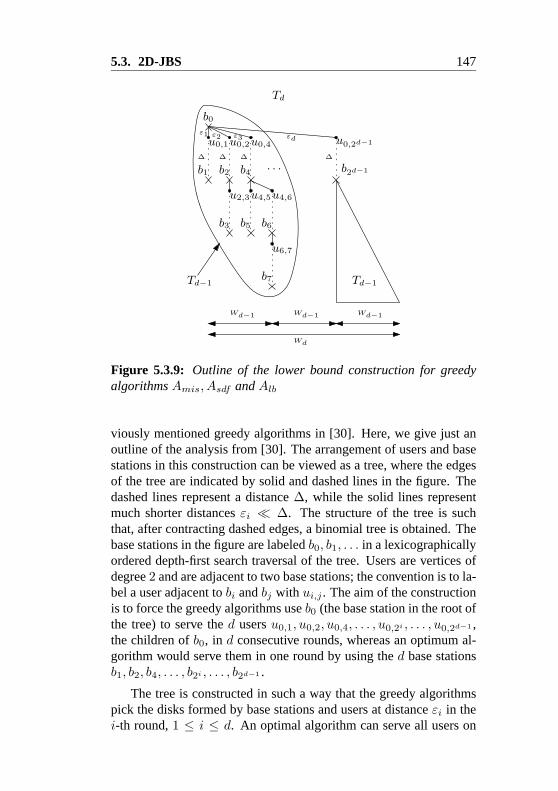
5.3. 2D-JBS 147
b0
b1 b2 b4
b3 b5 b6
b7
u0,1u0,2u0,4
u2,3u4,5u4,6
u6,7
ε1 ε2 ε3
∆ ∆ ∆
εd
∆
u0,2d−1
b2d−1
Td−1Td−1
Td
Wd−1 Wd−1 Wd−1
Wd
. . .
Figure 5.3.9: Outline of the lower bound construction for greedyalgorithms Amis, Asdf and Alb
viously mentioned greedy algorithms in [30]. Here, we give just anoutline of the analysis from [30]. The arrangement of users and basestations in this construction can be viewed as a tree, where the edgesof the tree are indicated by solid and dashed lines in the figure. Thedashed lines represent a distance ∆, while the solid lines representmuch shorter distances εi ∆. The structure of the tree is suchthat, after contracting dashed edges, a binomial tree is obtained. Thebase stations in the figure are labeled b0, b1, . . . in a lexicographicallyordered depth-first search traversal of the tree. Users are vertices ofdegree 2 and are adjacent to two base stations; the convention is to la-bel a user adjacent to bi and bj with ui,j . The aim of the constructionis to force the greedy algorithms use b0 (the base station in the root ofthe tree) to serve the d users u0,1, u0,2, u0,4, . . . , u0,2i , . . . , u0,2d−1 ,the children of b0, in d consecutive rounds, whereas an optimum al-gorithm would serve them in one round by using the d base stationsb1, b2, b4, . . . , b2i , . . . , b2d−1 .
The tree is constructed in such a way that the greedy algorithmspick the disks formed by base stations and users at distance εi in thei-th round, 1 ≤ i ≤ d. An optimal algorithm can serve all users on

148 Chapter 5. Joint Base Station Scheduling
some level in one round by using the base stations from below, atthe expense of blocking all users on level + 1. Thus, it can serveall users in two rounds by serving the odd levels in one round and theeven levels in the other. Consequently, the approximation ratio of thegreedy algorithms is Ω(d). The number nd of users in the tree Td canbe calculated by solving the simple recursion nd = 2nd−1 +1 (whichfollows from the recursive construction of the tree), where n1 = 1.This gives n = nd = 2d − 1 users and thus d = log (n + 1).
We formulate the lower bound for these greedy algorithms in thefollowing theorem (the proof can be found in [30]).
Theorem 5.25 There exist instances (U,B) of 2D-JBS in general po-sition for which the greedy algorithms Amis, Asdf and Alb have ap-proximation ratio Ω(log n), where n = |U |.
Note that algorithm Amis, which maximizes the number of servedusers in every round, achieves approximation ratio O(log n). This canbe shown by applying the standard analysis of the greedy set coveringalgorithm.

5.4. Conclusions and Open Problems 149
5.4 Conclusions and Open Problems
In this chapter we analyzed the 1D- and 2D-JBS problems that arise inthe context of coordinated scheduling in packet data systems. Theseproblems can be split into a selection and a coloring problem. In theone-dimensional case, we have shown that the coloring problem leadsto the class of arrow graphs, for which we have discussed its relationto other graph classes and algorithms. For the selection problem weproposed an approach based on LP relaxation with rounding. For the2D-problem, we have shown its NP-completeness.
The following problems remain still open:
• Is the 1D-JBS problem NP-complete or is there a polynomialtime algorithm that solves it?
• Are there constant approximation algorithms for the uncon-strained 2D-JBS problem?

150 Chapter 5. Joint Base Station Scheduling

Bibliography
[1] J. Adamek. Foundation of Coding. Wiley, 1991.
[2] F. Adashi, M. Sawahashi, and K. Okawa. Tree structured gen-eration of orthogonal spreading codes with different length forforward link of DS-CDMA mobile radio. Electronic Letters,33(1):27–28, January 1997.
[3] F. S. Al-Khaled. Optimal radio channel assignment through thenew binary dynamic simulated annealing algorithm. Interna-tional Journal of Communication Systems, (11):327–336, 1998.
[4] E. Amaldi, A. Capone, and F. Malucelli. Discrete modelsand algorithms for the capacitated location problems arising inUMTS network planning. Proceedings of the 5th internationalworkshop on Discrete algorithms and methods for mobile com-puting and communications, pages 1–8, 2001.
[5] R. Assarut, M. G. Husada, U. Yamamoto, and Y. Onozato.Data rate improvement with dynamic reassignment of spreadingcodes for DS-CDMA. Computer Communications, (25):1575–1583, 2002.
[6] R. Assarut, K. Kawanishi, R. Deshpande, U. Yamamoto, andY. Onozato. Performance evaluation of orthogonal variable-spreading-factor code assignment schemes in W-CDMA. ICC2002 conference, 2002.
[7] G. Ausiello, P. Crescenzi, G. Gambosi, V. Kann, A. Marchetti-Spaccamela, and M. Protasi. Complexity and Approximation.Springer, 1991.
151

152 Bibliography
[8] D. Beckmann and U. Killat. Frequency planning with respect tointerference minimization in cellular radio networks. Technicalreport, Vienna, Tech. Rep. COST259, 1999.
[9] D. Beckmann and U. Killat. A new strategy for the applicationof genetic algorithms to the channel-assignment problem. IEEETransactions on Vehicular Technology, 48(4):1261–1269, 1999.
[10] J. L. Bentley. Multidimensional divide-and-conquer. Commu-nications of the ACM, 23(4):214–229, 1980.
[11] M. Blum, R.W. Floyd, V. Pratt, R.L. Rivest, and R.E. Tarjan.Time bounds for selection. Journal of Computer and SystemSciences, 7, 1973.
[12] A. Brandstadt, V.B. Le, and J.P. Spinrad. Graph classes: A sur-vey. SIAM Monographs on Discrete Mathematics and Applica-tions. Society for Industrial and Applied Mathematics, Philadel-phia, PA, 1999.
[13] A.L. Buchsbaum and M.T. Goodrich. Three-Dimensional Lay-ers of Maxima. In Proceedings of the 10th Annual EuropeanSymposium on Algorithms (ESA’02), volume 2461, pages 257–269. Springer-Verlag, 2002.
[14] H. Cam. Nonblocking OVSF codes and enhancing network ca-pacity for 3G wireless and beyond systems. Intrenational Con-ference on Third Generation Wireless and Beyond, pages 148–153, Mai 2002.
[15] J.-C. Chen and W.-S. E. Chen. Implementation of an efficientchannelization code assignment algorithm in 3G WCDMA.2003.
[16] W. T. Chen and S. H. Fang. An efficient channelization codeassignment approach for W-CDMA. IEEE Conference on Wire-less LANs and Home Networks, 2002.
[17] W. T. Chen, Y. P. Wu, and H. C. Hsiao. A novel code assign-ment scheme for W-CDMA systems. Proc. of the 54th IEEEVehicular Technology Society Conference, 2:1182–1186, 2001.
[18] J. Chuzhoy and S. Naor. New hardness results for conges-tion minimization and machine scheduling. In Proceedings of

Bibliography 153
the 36th Annual ACM Symposium on the Theory of Computing(STOC’04), pages 28–34, 2004.
[19] M. Cielibak, T. Erlebach, F. Hennecke, B. Weber, and P. Wid-mayer. Scheduling jobs on a minimum number of machines. InProceedings of the 3rd IFIP International Conference on Theo-retical Computer Science, pages 217–230. Kluwer, 2004.
[20] S.A. Cook. The complexity of theorem-proving procedures.Proceedings of the 3rd Annual ACM Symposium on the Theoryof Computing (STOC’71), pages 151–158, 1971.
[21] S. Das, H. Viswanathan, and G. Rittenhouse. Dynamic load bal-ancing through coordinated scheduling in packet data systems.In Proceedings of Infocom’03, 2003.
[22] L. Davis. Handbook of Genetic Algorithms. New York: VanNostrand Reinhold, 1991.
[23] M. de Berg, M. van Kreveld, M. Overmars, andO. Schwarzkopf. Computational Geometry – Algorithmsand Applications. Springer, 2000.
[24] K. Deb, S. Agrawal, A. Pratap, and T. Meyarivan. A fast elitistnon-dominated sorting genetic algorithm for multi-objective op-timization: NSGA-II. in Parallel Problem Solving from Nature– PPSN VI, pages 849–858, 2000.
[25] K. Deb, A. Pratab, S. Agarwal, and T. Meyarivan. A fast andelitist multiobjective genetic algorithm: NSGA-II. IEEE Trans-actions on Evolutionary Computation, 6:182–197, April 2002.
[26] D.P. Dobkin and H. Edelsbrunner. Space searching for inter-secting objects. Journal of Algorithms, 8(5):348–361, 1987.
[27] M. Dorigo and T. Stutzle. Ant Colony Optimization. The MITPress, 2004.
[28] T. Erlebach, R. Jacob, M. Mihalak, M. Nunkesser, G. Szabo, andP. Widmayer. An algorithmic view on OVSF code assignment.TIK-Report 173, Computer Engineering and Networks Labora-tory (TIK), ETH Zurich, August 2003. Available electronicallyat ftp://ftp.tik.ee.ethz.ch/pub/publications/TIK-Report173.pdf.

154 Bibliography
[29] T. Erlebach, R. Jacob, M. Mihalak, M. Nunkesser, G. Szabo, andP. Widmayer. An algorithmic view on OVSF code assignment.in Proc. of the 21st Annual Symposium on Theoretical Aspectsof Computer Science, 2004.
[30] T. Erlebach, R. Jacob, M. Mihalak, M. Nunkesser, G. Szabo,and P. Widmayer. Joint base station scheduling. Technical Re-port 461, ETH Zrich Institute of Theoretical Computer Science,2004.
[31] T. Erlebach, R. Jacob, M. Mihalak, M. Nunkesser, G. Szabo,and P. Widmayer. Joint Base Station Scheduling. in Proc. ofthe 2nd International Workshop on Approximation and OnlineAlgorithms, 2004.
[32] T. Erlebach and F.C.R. Spieksma. Interval selection: Applica-tions, algorithms, and lower bounds. Algorithmica, 46:27–53,2001.
[33] R. Fantacci and S. Nannicini. Multiple access protocol for in-tegration of variable bit rate multimedia traffic in UMTS/IMT-2000 based on wideband CDMA. IEEE Journal on SelectedAreas in Communications, 18(8):1441–1454, August 2000.
[34] S. Felsner, R. Muller, and L. Wernisch. Trapezoid graphs andgeneralizations, geometry and algorithms. Discrete AppliedMathematics, 74:13–32, 1997.
[35] M. Fischetti, C. Lepschy, G. Minerva, G. Romanin-Jacur, andE. Toto. Frequency assignment in mobile radio systems usingbranch-and-cut techniques. European Journal of OperationalResearch, 123:241–255, 2000.
[36] L. C. P. Floriani and G. R. Mateus. An optimization model forthe bst location problem in outdoor cellular and pcs systems.in Proceedings of the 15th International Teletraffic Congress,1997.
[37] C. M. Fonseca and P. J. Fleming. Genetic algorithms for mul-tiobjective optimization: Formulation, discussion and general-ization. in Proc. of the Fifth Int. Conf. on Genetic Algorithms,pages 416–423, 1993.

Bibliography 155
[38] C. E. Fossa Jr. Dynamic Code Sharing Algorithms for IP Qual-ity of Service in Wideband CDMA 3G Wireless Networks. PhDthesis, Virginia Polytechnic Institute and State University, April2002.
[39] C. E. Fossa Jr and N. J. Davis IV. Dynamic code assignment im-proves channel utilization for bursty traffic in 3G wireless net-works. IEEE International Communications Conference, 2002.
[40] G.N. Frederickson and S. Rodger. A new approach to the dy-namic maintenance of maximal points in a plane. Discrete Com-putational Geometry, 5(4):365–374, 1990.
[41] M. Galota, C. Glasser, S. Reith, and H. Vollmer. A polynomial-time approximation scheme for base station positioning inUMTS networks. in Proceedings 5th Discrete Algorithms andMethods for Mobile Computing and Communications, pages52–59, 2000.
[42] M. R. Garey and D. S. Johnson. Computers and Intractability.Freeman, 1979.
[43] C. Glasser, S. Reith, and H. Vollmer. The complexity of basestation positioning in cellular networks. in ICALP SatelliteWorkshops, pages 167–178, 2000.
[44] A. Graf, M. Stumpf, and G. Weienfels. On coloring unit diskgraphs. Algorithmica, 20(3):277–293, March 1998.
[45] M. Grotschel, L. Lovasz, and A. Schrijver. The ellipsoidmethod and its consequences in combinatorial optimization.Combinatorica, 1:169–197, 1981.
[46] J.M. Hernando and F. Perez-Fontan. Introduction to Mo-bile Communications Engineering. Artech House Publishers,Boston/London, 1999.
[47] H. Holma and A. Toskala. WCDMA for UMTS. Wiley, 2001.
[48] J. Horn, N. Nafpliotis, and D. E. Goldberg. A niched paretoalgorithm for multiobjective optimization. in Proc. of the FirstIEEE Conf. on Evolutionary Computation, 1:82–87, 1994.

156 Bibliography
[49] R. Janardan. On the Dynamic Maintenance of Maximal Pointsin the Plane. Information Processing Letters, 40(2):59–64,1991.
[50] B. Jaumard, O. Marcotte, and C. Meyer. Mathematical mod-els and exact methods for channel assignment in cellular net-works. in Telecommunications Network Planning, chapter 13,pages 239–255, 1999.
[51] M.T. Jensen. Reducing the Run-Time Complexity of Multiob-jective EAs: The NSGA-II and Other Algorithms. IEEE Trans-actions on Evolutionary Computation, 7(5):503–515, October2003.
[52] J. Kalvenes and R. Gupta. Hierarchical cellular network designwith channel allocation. Informs Select Proceedings of the 2000Telecommunications Conference, 2000.
[53] B. Kalyanasundaram and K. Pruhs. Speed is as powerful asclairvoyance [scheduling problems]. Proceedings of the 36thIEEE Symposium on Foundations of Computer Science, pages214–221, 1995.
[54] B. Kalyanasundaram and K. Pruhs. Speed is as powerful asclairvoyance. J. ACM, 47(4):617–643, 2000.
[55] A. C. Kam, T. Minn, and K.-Y. Siu. Supporting rate guaranteeand fair access for bursty data traffic in W-CDMA. IEEE Jour-nal on Selected Areas in Communications, 19(11):2121–2130,November 2001.
[56] S. Kapoor. Dynamic Maintenance of Maxima of 2-d Point Sets.SIAM J. Comput., 29(6):1858–1877, 2000.
[57] R.M. Karp. Reducibility among combinatorial problems. inComplexity of Computer Computations, pages 85–103, 1972.
[58] L.G. Khachiyan. A polynomial algorithm in linear program-ming. Doklady Akademii Nauk SSSR, 244:1093–1096, 1979.
[59] H.T. Kung, F. Luccio, and F.P. Preparata. On finding the max-ima of a set of vectors. Journal of the ACM, 22(4):469–476,October 1975.

Bibliography 157
[60] J. Laiho, A. Wacker, and T. Novosad. Radio Network Planningand Optimisation for UMTS. Wiley, New York, 2002.
[61] L.A. Levin. Universal Sorting Problems. Problems of Informa-tion Transmission, 9:265–266, 1973.
[62] K. Mehlhorn and S. Naher. Dynamic Fractional Cascading. Al-gorithmica, 5:215–241, 1990.
[63] K. Mehlhorn and S. Naher. The LEDA platform of combinato-rial and geometric computing. 1999.
[64] T. Minn and K. Y. Siu. Dynamic assignment of orthogonalvariable-spreading-factor codes in W-CDMA. IEEE Journal onselected areas in communications, 18(8):1429–1440, 2000.
[65] L. Monier. Combinatorial Solutions of MultidimensionalDivide-and-Conquer Recurrences. Journal of Algorithms,1:60–74, 1980.
[66] M.H. Overmars and J. Van Leeuwen. Maintenance of Configu-rations in the Plane. Journal of Computer and System Sciences,23:166–204, 1981.
[67] C.H. Papadimitriou. Computational Complexity. Addison-Wesley, 1994.
[68] V. Pareto. Cours d’economie politique. 1896.
[69] B. J. Ritzel, J. W. Eheart, and S. Ranjithan. Using genetic al-gorithms to solve a multiple objective groundwater pollutioncontainment problem. Water Resources Research, 30(5):1589–1603, 1994.
[70] P. Ross, D. Corne, and H.-L. Fang. Improving evolutionarytimetabling with delta evaluation and directed mutation. in Par-allel Problem Solving from Nature – PPSN III, LNCS 866:556–565, 1994.
[71] A. N. Rouskas and D. N. Skoutas. OVSF codes assignmentand reassignment at the forward link of W-CDMA 3G systems.PIMRC 2002, 2002.

158 Bibliography
[72] J. D. Schaffer. Multiple objective optimization with vector eval-uated genetic algorithms. in Proc. of the First Int. Conf. on Ge-netic Algorithms, pages 93–100, 1985.
[73] F.C.R. Spieksma. On the approximability of an intervalscheduling problem. Journal of Scheduling, 2:215–227, 1999.
[74] J.P. Spinrad. Efficient Graph Representations, volume 19 ofField Institute Monographs. AMS, 2003.
[75] N. Srinivas and K. Deb. Multiobjective optimization using non-dominated sorting in genetic algorithms. Evolutionary Compu-tation, 2(3):221–248, 1995.
[76] G.L. Stuber. Principels of Mobile Communication. KluwerAcademic Publishers, Boston, 1996.
[77] G. Syswerda and J. Palmucci. The application of genetic algo-rithms to resource scheduling. in Proc. of the Fourth Int. Conf.on Genetic Algorithms, pages 502–508, 1991.
[78] M. Tomamichel. Algorithmische Aspekte von OVSF CodeAssignment mit Schwerpunkt auf Offline Code Assignmnent.Semester thesis, Computer Engineering and Networks Labora-tory (TIK), ETH Zurich, 2004.
[79] K. Tutschku, T. Leskien, and P. Tran-Gia. Traffic estimationand characterization for the design of mobile communicationnetworks. Technical report, University of Wurzburg Institute ofComputer Science, 1997.
[80] K. Tutschku, R. Mathar, and T. Niessen. Interference minimiza-tion in wireless communciation systems by optimal cell site se-lection. in Proceedings EPMCC’99, pages 208–213, 1999.
[81] P. van Emde Boas, R. Kaas, and E. Zijlstra. Design and Imple-mentation of an Efficient Priority Queue. Mathematical SystemsTheory, 10:99–127, 1977.
[82] J. van Leeuwen. Handbook of Theoretical Computer Science.Elsevier Science Publisher, Amsterdam, 1990.
[83] D. A. Van Veldhuizen and G. B. Lamont. Multiobjective opti-mization with messy genetic algorithms. in Proceedings of the

Bibliography 159
2000 ACM Symposium on Applied Computing, pages 470–476,2000.
[84] V.V. Vazirani. Approximation Algorithms. Springer, 2001.
[85] N. Weicker. Qualitative No Free Lunch Aussagen fur Evolu-tionare Algorithmen. Gottingen: Cuvillier, 2001.
[86] N. Weicker, G. Szabo, K. Weicker, and P. Widmayer. Evolu-tionary Multiobjective Optimization for Base Station Transmit-ter Placement with Frequency Assignment. IEEE Transactionson Evolutionary Computation, 7(2):189–203, 2003.
[87] D. West. Introduction to Graph Theory. Prentice Hall, 2ndedition, 2001.
[88] D. H. Wolpert and W. G. Macready. No free lunch theoremsfor optimization. IEEE Trans. on Evolutionary Computation,1(1):67–82, 1997.
[89] F.F. Yao. On finding the maximal elements in a set of plane vec-tors. Technical report, Computer Science Dep. Rep., Universityof Illinois at Urbana-Champaign, 1974.
[90] T. Yu and P. Bentley. Methods to evolve legal phenotypes.in Parallel Problem Solving from Nature – PPSN V, LNCS1498:280–291, 1998.
[91] X. Zhou and T. Nishizeki. Efficient algorithms for weightedcolorings of series-parallel graphs. in 12th International Sym-posium on Algorithms and Computation, pages 514–524, 2001.
[92] E. Zitzler, M. Laumanns, and L. Thiele. SPEA2: Improving thestrength pareto evolutionary algorithm for multiobjective opti-mization. in Proceedings of Evolutionary Methods for Design,Optimisation and Control, 2002.
[93] E. Zitzler and L. Thiele. Multiobjective evolutionary algo-rithms: A comparative case study and the strength Paretoapproach. IEEE Transactions on Evolutionary Computation,3(4):257–271, 1999.

160 Bibliography
[94] E. Zitzler and L. Thiele. Multiobjective evolutionary algo-rithms: A comparative case study and the strength pareto ap-proach. IEEE Transactions on Evolutionary Computation,3:257–271, November 1999.

Curriculum VitaeGabor Vilmos Szabo
born on December 19, 1976 in Zalau, Romania
1991–1995 High school in Zalau, Romania
1995–2000 Studies at the Technical University of Cluj-Napoca,RomaniaComputer ScienceDegree: Bachelor in Computer Science
2000–2005 PhD student at Swiss Federal Institute of Technol-ogy, SwitzerlandTheoretical Computer Science