optimization problems arising -...

Home Page

Title Page

Contents

JJ II

J I

of 31

Go Back

Full Screen

Close

Quit

Optimization Problems Arising

in Optics and Mechanics

Robert J. Vanderbei

October 1, 2004Center for Applied Mathematics

Cornell UniversityIthaca NY

Member: Princeton University/Ball Aerospace TPF Team

http://www.princeton.edu/∼rvdb

http://www.princeton.edu/~rvdb


Home Page

Title Page

Contents

JJ II

J I

of 31

Go Back

Full Screen

Close

Quit

1. Optimization

minimize f (x)subject to b ≤ h(x) ≤ b + r,

l ≤ x ≤ u

• Linear Programming (LP): f and h are linear.

• Convex Optimization: f is convex, each hi is concave, and r = ∞.

• Nonlinear Optimization: f and each hi is assumed to be twicedifferentiable

• Generally, we seek a local solution in the vicinity of a given startingpoint.

• If problem is convex (which includes LP), any local solution is au-tomatically a global solution.


Home Page

Title Page

Contents

JJ II

J I

of 31

Go Back

Full Screen

Close

Quit

2. The Big Question: Are We Alone?

• Are there Earth-likeplanets?

• Are they common?

• Is there life on some ofthem?


Home Page

Title Page

Contents

JJ II

J I

of 31

Go Back

Full Screen

Close

Quit

3. Exosolar Planets—Where We Are Now

There are more than 120 Exosolar planets known today.

They were discovered by detecting a sinusoidaldoppler shift in the parent star’s spectrum dueto gravitationally induced wobble.

This method works best for large Jupiter-sized planets with close-inorbits.

One of these planets, HD209458b, also transits its parent star onceevery 3.52 days. These transits have been detected photometrically asthe star’s light flux decreases by about 1.5% during a transit.

Recent transit spectroscopy of HD209458b shows it is a gas giant.


Home Page

Title Page

Contents

JJ II

J I

of 31

Go Back

Full Screen

Close

Quit

4. Future Exosolar Planet Missions

• 2006, Kepler a space-based telescope tomonitor 100,000 stars simultaneously look-ing for “transits”.

• 2007, Eclipse a space-based telescope to di-rectly image Jupiter-like planets.

• 2009, Space Interferometry Mission (SIM)will look for astrometric wobble.

• 2014, Darwin is a space-based cluster of 6 telescopes used as aninterferometer.

• 2014, Terrestrial Planet Finder (TPF) space-based telescope to di-rectly image Earth-like planets.


Home Page

Title Page

Contents

JJ II

J I

of 31

Go Back

Full Screen

Close

Quit

5. Terrestrial Planet Finder Telescope

• DETECT: Search 150-500 nearby (5-15 pc distant) Sun-like starsfor Earth-like planets.

• CHARACTERIZE: Determine basic physical properties and measure“biomarkers”, indicators of life or conditions suitable to support it.


Home Page

Title Page

Contents

JJ II

J I

of 31

Go Back

Full Screen

Close

Quit

6. Why Is It Hard?

• If the star is Sun-like and the planet is Earth-like, then the reflectedvisible light from the planet is 10−10 times as bright as the star.This is a difference of 25 magnitudes!

• If the star is 10 pc (33 ly) away and the planet is 1 AU from thestar, the angular separation is 0.1 arcseconds!

Originally, it was thought that this wouldrequire a space-based infrared nulling inter-ferometer (as shown).

However, a more recent idea is to use asingle large visible-light telescope with anelliptical mirror (4 m x 10 m) and a shapedpupil for diffraction control.


Home Page

Title Page

Contents

JJ II

J I

of 31

Go Back

Full Screen

Close

Quit

7. The Shaped Pupil Concept

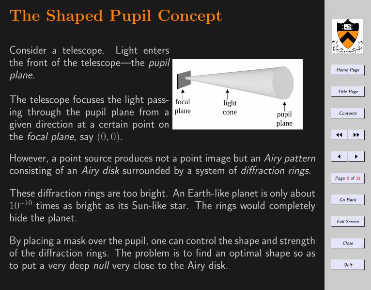
Consider a telescope. Light entersthe front of the telescope—the pupilplane.

The telescope focuses the light pass-ing through the pupil plane from agiven direction at a certain point onthe focal plane, say (0, 0).

focal plane

light cone pupil

plane

However, a point source produces not a point image but an Airy patternconsisting of an Airy disk surrounded by a system of diffraction rings.

These diffraction rings are too bright. An Earth-like planet is only about10−10 times as bright as its Sun-like star. The rings would completelyhide the planet.

By placing a mask over the pupil, one can control the shape and strengthof the diffraction rings. The problem is to find an optimal shape so asto put a very deep null very close to the Airy disk.


Home Page

Title Page

Contents

JJ II

J I

of 31

Go Back

Full Screen

Close

Quit

The Shaped Pupil Concept

Consider a telescope. Light entersthe front of the telescope—the pupilplane.

The telescope focuses the light pass-ing through the pupil plane from agiven direction at a certain point onthe focal plane, say (0, 0).

focal plane

light cone pupil

plane

However, a point source produces not a point image but an Airy patternconsisting of an Airy disk surrounded by a system of diffraction rings.

These diffraction rings are too bright. An Earth-like planet is only about10−10 times as bright as its Sun-like star. The rings would completelyhide the planet.

By placing a mask over the pupil, one can control the shape and strengthof the diffraction rings. The problem is to find an optimal shape so asto put a very deep null very close to the Airy disk.


Home Page

Title Page

Contents

JJ II

J I

of 31

Go Back

Full Screen

Close

Quit

8. The Airy Pattern

-30 -20 -10 0 10 20 30-140

-120

-100

-80

-60

-40

-20

0


Home Page

Title Page

Contents

JJ II

J I

of 31

Go Back

Full Screen

Close

Quit

9. The Princeton Team

David Spergel (Astrophysics, MacArthur genius, Time’s astrophysicistof the 21st century, ...)

Jeremy Kasdin (Aerospace Engineering, Gravity Probe-B chief systemsengineer)

Robert Vanderbei (the Optimization guy)

Other Princeton members: M. Littman, E. Turner, J. Gunn, M. Carr

And, other members from JPL, Ball Aerospace, and Harvard Center for Astrophysics


Home Page

Title Page

Contents

JJ II

J I

of 31

Go Back

Full Screen

Close

Quit

10. Electric Field

The image-plane electric field E() produced by an on-axis plane waveand an apodized aperture defined by an apodization function A() isgiven by

E(ξ, ζ) =

∫ 1/2

−1/2

∫ 1/2

−1/2ei(xξ+yζ)A(x, y)dydx

...

E(ρ) = 2π

∫ 1/2

0J0(rρ)A(r)rdr,

where J0 denotes the 0-th order Bessel function of the first kind.

The unitless pupil-plane “length” r is given as a multiple of the apertureD.

The unitless image-plane “length” ρ is given as a multiple of focal-length times wavelength over aperture (fλ/D) or, equivalently, as anangular measure on the sky, in which case it is a multiple of just λ/D.(Example: λ = 0.5µm and D = 10m implies λ/D = 10mas.)

The intensity is the square of the electric field.


Home Page

Title Page

Contents

JJ II

J I

of 31

Go Back

Full Screen

Close

Quit

11. Performance Metrics

Inner and Outer Working Angles

ρiwa ρowa

Contrast:E2(ρ)/E2(0)

Airy Throughput:∫ ρiwa

0E2(ρ)2πρdρ

(π(1/2)2)= 8

∫ ρiwa

0E2(ρ)ρdρ.


Home Page

Title Page

Contents

JJ II

J I

of 31

Go Back

Full Screen

Close

Quit

12. Clear Aperture—Airy Pattern

ρiwa = 1.24 TAiry = 84.2% Contrast = 10−2

-40 -30 -20 -10 0 10 20 30 40-140

-120

-100

-80

-60

-40

-20

0


Home Page

Title Page

Contents

JJ II

J I

of 31

Go Back

Full Screen

Close

Quit

13. Optimization

Find apodization function A() that solves:

maximize

∫ 1/2

0A(r)2πrdr

subject to −10−5E(0) ≤E(ρ)≤ 10−5E(0), ρiwa ≤ ρ ≤ ρowa,

0 ≤ A(r)≤ 1, 0 ≤ r ≤ 1/2,

Note similarity to FIR filter design and antenna array design problems.


Home Page

Title Page

Contents

JJ II

J I

of 31

Go Back

Full Screen

Close

Quit

Apodization

ρiwa = 4 TAiry = 9%

Excellent dark zone. Unmanufacturable.

-0.5 -0.4 -0.3 -0.2 -0.1 0 0.1 0.2 0.3 0.4 0.50

0.1

0.2

0.3

0.4

0.5

0.6

0.7

0.8

0.9

1

-60 -40 -20 0 20 40 60-180

-160

-140

-120

-100

-80

-60

-40

-20

0


Home Page

Title Page

Contents

JJ II

J I

of 31

Go Back

Full Screen

Close

Quit

14. Masks

Consider a binary apodization (i.e., a mask) consisting of an openinggiven by

A(x, y) =

{1 |y| ≤ a(x)0 else

We only consider masks that are symmetric with respect to both the xand y axes. Hence, the function a() is a nonnegative even function.

In such a situation, the electric field E(ξ, ζ) is given by

E(ξ, ζ) =

∫ 12

−12

∫ a(x)

−a(x)ei(xξ+yζ)dydx

= 4

∫ 12

0cos(xξ)

sin(a(x)ζ)

ζdx


Home Page

Title Page

Contents

JJ II

J I

of 31

Go Back

Full Screen

Close

Quit

15. Maximizing Throughput

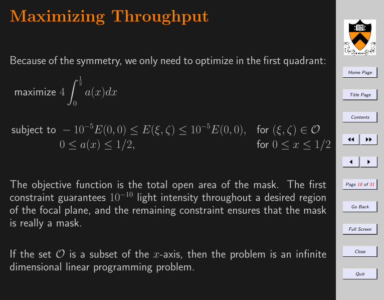
Because of the symmetry, we only need to optimize in the first quadrant:

maximize 4

∫ 12

0a(x)dx

subject to − 10−5E(0, 0) ≤ E(ξ, ζ) ≤ 10−5E(0, 0), for (ξ, ζ) ∈ O0 ≤ a(x) ≤ 1/2, for 0 ≤ x ≤ 1/2

The objective function is the total open area of the mask. The firstconstraint guarantees 10−10 light intensity throughout a desired regionof the focal plane, and the remaining constraint ensures that the maskis really a mask.

If the set O is a subset of the x-axis, then the problem is an infinitedimensional linear programming problem.


Home Page

Title Page

Contents

JJ II

J I

of 31

Go Back

Full Screen

Close

Quit

16. One Pupil w/ On-Axis Constraints

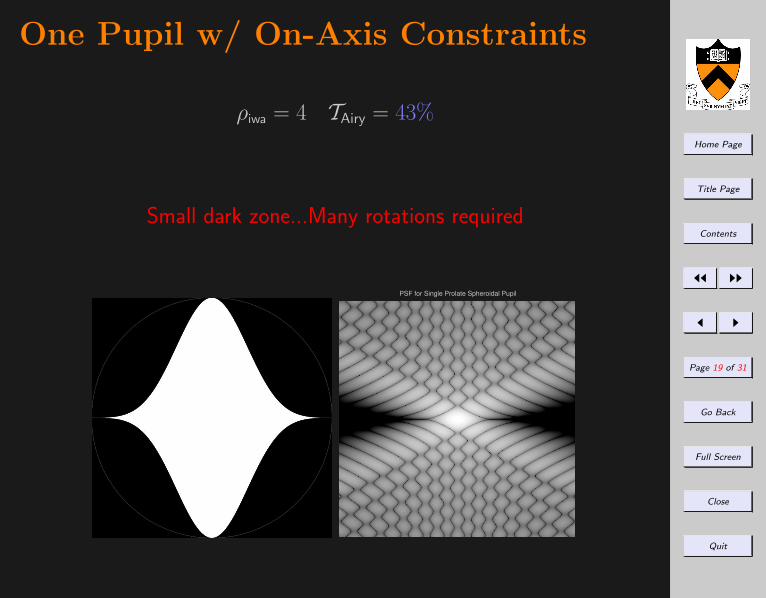
ρiwa = 4 TAiry = 43%

Small dark zone...Many rotations required

PSF for Single Prolate Spheroidal Pupil


Home Page

Title Page

Contents

JJ II

J I

of 31

Go Back

Full Screen

Close

Quit

17. Multiple Pupil Mask

ρiwa = 4

TAiry = 30%

Throughput relative to ellipse11% central obstr.

Easy to makeVery few rotations


Home Page

Title Page

Contents

JJ II

J I

of 31

Go Back

Full Screen

Close

Quit

18. Concentric Ring Masks

Recall that for circularly symmetric apodizations

E(ρ) = 2π

∫ 1/2

0J0(rρ)A(r)rdr,

where J0 denotes the 0-th order Bessel function of the first kind.

Let

A(r) =

{1 r2j ≤ r ≤ r2j+1, j = 0, 1, . . . ,m− 10 otherwise,

where0 ≤ r0 ≤ r1 ≤ · · · ≤ r2m−1 ≤ 1/2.

The integral can now be written as a sum of integrals and each of theseintegrals can be explicitly integrated to get:

E(ρ) =

m−1∑j=0

1

ρ

(r2j+1J1

(ρr2j+1

)− r2jJ1

(ρr2j

)).


Home Page

Title Page

Contents

JJ II

J I

of 31

Go Back

Full Screen

Close

Quit

Optimization Problem

maximizem−1∑j=0

π(r22j+1 − r2

2j)

subject to: − 10−5E(0) ≤ E(ρ) ≤ 10−5E(0), for ρ0 ≤ ρ ≤ ρ1

where E(ρ) is the function of the rj’s given on the previous slide.

This problem is a semiinfinite nonconvex optimization problem.


Home Page

Title Page

Contents

JJ II

J I

of 31

Go Back

Full Screen

Close

Quit

Concentric Ring Mask

ρiwa = 4 ρowa = 60

TAiry = 9%

Lay it on glass?No rotations

0 10 20 30 40 50 60 70 80 90 10010

-15

10-10

10-5

100


Home Page

Title Page

Contents

JJ II

J I

of 31

Go Back

Full Screen

Close

Quit

19. Optimization Success Story

From an April 12, 2004, letter from Charles Beichman:Dear TPF-SWG,

I am writing to inform you of exciting new developments for TPF. As part of the Presidents new visionfor NASA, the agency has been directed by the President to conduct advanced telescope searches forEarth-like planets and habitable environments around other stars. Dan Coulter, Mike Devirian, and Ihave been working with NASA Headquarters (Lia LaPiana, our program executive; Zlatan Tsvetanov,our program scientist; and Anne Kinney) to incorporate TPF into the new NASA vision. The resultof these deliberations has resulted in the following plan for TPF:

1. Reduce the number of architectures under study from four to two: (a) the moderate sizedcoronagraph, nominally the 4x6 m version now under study; and (b) the formation flying inter-ferometer presently being investigated with ESA. Studies of the other two options, the large, 10-12m, coronagraph and the structurally connected interferometer, would be documented and brought toa rapid close.

2. Pursue an approach that would result in the launch of BOTH systems within the next 10-15years. The primary reason for carrying out two missions is the power of observations at IR and visiblewavelength regions to determine the properties of detected planets and to make a reliable and robustdetermination of habitability and the presence of life.

3. Carry out a modest-sized coronagraphic mission, TPF-C, to be launched around 2014,to be followed by a formation-flying interferometer, TPF-I, to be conducted jointly with ESA andlaunched by the end of decade (2020). This ordering of missions is, of course, subject to the readinessof critical technologies and availability of funding. But in the estimation of NASA HQ and the project,the science, the technology, the political will, and the budgetary resources are in place to support thisplan.

...

The opportunity to move TPF forward as part of the new NASA vision has called for these rapid anddramatic actions. What has made these steps possible has been the hard work by the entire team,including the TPF-SWG, the two TPF architecture teams, and all the technologists at JPL and aroundthe country, which has demonstrated that NASA is ready to proceed with both TPF-C and TPF-Iand that the data from these two missions are critical to the success of the goals of TPF. We will bemaking more information available as soon as additional details become available. Thank you for allyour help in preparing TPF to take advantage of this opportunity.


Home Page

Title Page

Contents

JJ II

J I

of 31

Go Back

Full Screen

Close

Quit

20. Least Action Principle

Given: n bodies.

Let:mj denote the mass andzj(t) denote the position in R2 = C of body j at time t.

Action Functional:

A =

∫ 2π

0

∑j

mj

2‖zj‖2 +

∑j,k:k<j

mjmk

‖zj − zk‖

dt.


Home Page

Title Page

Contents

JJ II

J I

of 31

Go Back

Full Screen

Close

Quit

21. Equation of Motion

First Variation:

δA =

∫ 2π

0

∑α

∑j

mjzαj δz

α

j −∑

j,k:k<j

mjmk

(zαj − zα

k )(δzαj − δzα

k )

‖zj − zk‖3

dt

= −∫ 2π

0

∑j

∑α

mjzαj +

∑k:k 6=j

mjmk

zαj − zα

k

‖zj − zk‖3

δzαj dt

Setting first variation to zero, we get:

mjzαj = −

∑k:k 6=j

mjmk

zαj − zα

k

‖zj − zk‖3, j = 1, 2, . . . , n, α = 1, 2

Note: If mj = 0 for some j, then the first order optimality conditionreduces to 0 = 0, which is not the equation of motion for a masslessbody.


Home Page

Title Page

Contents

JJ II

J I

of 31

Go Back

Full Screen

Close

Quit

22. Periodic Solutions

We assume solutions can be expressed in the form

zj(t) =

∞∑k=−∞

γkeikt, γk ∈ C.

Writing with components zj(t) = (xj(t), yj(t)) and γk = (αk, βk), weget

x(t) = a0 +

∞∑k=1

(ac

k cos(kt) + ask sin(kt)

)y(t) = b0 +

∞∑k=1

(bck cos(kt) + bs

k sin(kt))

where

a0 = α0, ack = αk + α−k, as

k = β−k − βk,

b0 = β0, bck = βk + β−k, bs

k = αk − α−k.

The variables a0, ack, as

k, b0, bck, and bs

k are the decision variables in theoptimization model.


Home Page

Title Page

Contents

JJ II

J I

of 31

Go Back

Full Screen

Close

Quit

23. The ampl Model

param N := 3; # number of massesparam n := 15; # number of terms in Fourier series representationparam m := 100; # number of terms in numerical approx to integral

param theta {j in 0..m-1} := j*2*pi/m;

param a0 {i in 0..N-1} default 0; param b0 {i in 0..N-1} default 0;var as {i in 0..N-1, k in 1..n} := 0; var bs {i in 0..N-1, k in 1..n} := 0;var ac {i in 0..N-1, k in 1..n} := 0; var bc {i in 0..N-1, k in 1..n} := 0;

var x {i in 0..N-1, j in 0..m-1}= a0[i]+sum {k in 1..n} ( as[i,k]*sin(k*theta[j]) + ac[i,k]*cos(k*theta[j]) );

var y {i in 0..N-1, j in 0..m-1}= b0[i]+sum {k in 1..n} ( bs[i,k]*sin(k*theta[j]) + bc[i,k]*cos(k*theta[j]) );

var xdot {i in 0..N-1, j in 0..m-1}= if (j<m-1) then (x[i,j+1]-x[i,j])*m/(2*pi) else (x[i,0]-x[i,m-1])*m/(2*pi);

var ydot {i in 0..N-1, j in 0..m-1}= if (j<m-1) then (y[i,j+1]-y[i,j])*m/(2*pi) else (y[i,0]-y[i,m-1])*m/(2*pi);

var K {j in 0..m-1} = 0.5*sum {i in 0..N-1} (xdot[i,j]^2 + ydot[i,j]^2);

var P {j in 0..m-1}= - sum {i in 0..N-1, ii in 0..N-1: ii>i}

1/sqrt((x[i,j]-x[ii,j])^2 + (y[i,j]-y[ii,j])^2);

minimize A: (2*pi/m)*sum {j in 0..m-1} (K[j] - P[j]);


Home Page

Title Page

Contents

JJ II

J I

of 31

Go Back

Full Screen

Close

Quit

Continued...

let {i in 0..N-1, k in 1..n} as[i,k] := 1*(Uniform01()-0.5);let {i in 0..N-1, k in 1..n} ac[i,k] := 1*(Uniform01()-0.5);let {i in 0..N-1, k in n..n} bs[i,k] := 0.01*(Uniform01()-0.5);let {i in 0..N-1, k in n..n} bc[i,k] := 0.01*(Uniform01()-0.5);

solve;


Home Page

Title Page

Contents

JJ II

J I

of 31

Go Back

Full Screen

Close

Quit

24. Choreographies and the Ducati

The previous ampl model was used to find many choreographies (a laMoore and Montgomery/Chencinier) in the equimass n-body problemand the stable Ducati solution to the 3-body problem.

-1.5

-1

-0.5

0

0.5

1

1.5

-1.5 -1 -0.5 0 0.5 1 1.5

"after.out"


C:/user/rvdb/public_html/JAVA/astro/galaxy/periodicOrbits/papers/braid/braid3.ps

Home Page

Title Page

Contents

JJ II

J I

of 31

Go Back

Full Screen

Close

Quit

Contents1 Optimization 2

2 The Big Question: Are We Alone? 3

3 Exosolar Planets—Where We Are Now 4

4 Future Exosolar Planet Missions 5

5 Terrestrial Planet Finder Telescope 6

6 Why Is It Hard? 7

7 The Shaped Pupil Concept 8

8 The Airy Pattern 10

9 The Princeton Team 11

10 Electric Field 12

11 Performance Metrics 13

12 Clear Aperture—Airy Pattern 14

13 Optimization 15

14 Masks 17

15 Maximizing Throughput 18

16 One Pupil w/ On-Axis Constraints 19

17 Multiple Pupil Mask 20

18 Concentric Ring Masks 21

19 Optimization Success Story 24

20 Least Action Principle 25

21 Equation of Motion 26

22 Periodic Solutions 27

23 The ampl Model 28

24 Choreographies and the Ducati 30


optimization problems arising -...

Documents