optimization of fuel efficiency of a hybrid …€¦ · the aim of this project is to optimize the...
TRANSCRIPT

`
OPTIMIZATION OF FUEL EFFICIENCY OF A HYBRID ELECTRIC BUS
By
Govind Menon
Jonathan Verghese
Karan Shah
Shanker Krishnan
MAE 598-2015-11
Final Report
ABSTRACT
A bus is one of the most popular and widely used modes of public
transportation. It is also one of the main contributors of CO2 emissions. An
estimated 4400kg/person/year of CO2 is emitted by a bus in the United States of
America alone. From this it is imperative that a more eco-friendly version of the
bus is the need of the hour. Although the use of hybrid electric powertrains has
been comparatively more popular in the light motor vehicle category, the use
of such technology is not predominantly found in urban transit buses. We aim to
shorten this gap with this project.
The aim of this project is to optimize the hybrid electric system to minimize the
fuel consumption. The project involves optimization process of mainly 3
subsystems. These include a) the mechanical coupler, b) the optimal control
and c) the battery sizing, all of which play a crucial role in determining the
mileage of the bus. The modelling of this problem is done by collecting the drive
cycle data of a bus and doing the necessary modelling using MATLAB. The final
mpg value obtained is 7.5 which is noticeably better than a regular transit bus
which has a mpg value of 4.03(orange county drive cycle). The subsystem
optimization values from the mechanical coupler and the battery subsystem are
fed into the optimal control code to find the overall system optimization.

`
ACKNOWLEDGEMENT
This is a special acknowledgment to Dr. Yi Ren , Dr Emrah Bayrak and Dr . Panos
Y Papalambros whose technical paper on “Design of hybrid-electric vehicle
architectures using Auto-generation of feasible driving modes “helped us
complete the optimal control subsystem . We would like to specially thank Dr Yi
Ren for the help and guidance that he provided us.
`
TABLE OF CONTENTS
1. Design Problem Statement
2. Nomenclature
2.1 Nomenclature – A (Battery Subsystem)
2.2 Nomenclature – B (Mechanical Coupler Subsystem)
2.3 Nomenclature – C (Optimal Control Subsystem)
3. Battery Subsystem
3.1 Mathematical Model
3.2 Model Analysis
3.3 Optimization Study
3.4 Parametric Study
3.5 Discussion of Results
4. Mechanical Coupler Subsystem
4.1 Mathematical Model
4.2 Model Analysis
4.3 Optimization Study
4.4 Parametric Study
4.5 Discussion of Results
5. Optimal Control Subsystem
5.1 Mathematical Model
5.2 Model Analysis
5.3 Basic flow of the program
5.4 Optimization study
5.5 Discussion of Results
6. System Integration Study
7. References
8. Appendices
8.1 Appendix – A (Battery Subsystem
8.2 Appendix – B (Mechanical Coupler Subsystem)
8.3 Appendix – C (Optimal Control Subsystem)
8.4 Appendix – D (System Integration)

`
1. DESIGN PROBLEM STATEMENT
The objective of the project is to optimize of fuel efficiency for a hybrid electric
bus operating in urban driving conditions as per a specific urban drive cycle
observed. The hybrid electric bus taken into consideration has a parallel
architecture powered by a single internal combustion engine and single motor
configuration whose outputs are coupled by a mechanical coupler.
The global objective of optimization of the fuel efficiency is further sub-divided
into individual subsystems which are the battery subsystem, the mechanical
coupler subsystem and optimal control subsystem and they have their
respective objectives. The optimum results obtained from the individual
subsystems are integrated into a common objective function which depends on
the design variables and parameters from all the three subsystems to obtain the
optimal solution for the fuel efficiency of the hybrid electric bus.
The objective of the Battery subsystem is to maximize the power generated by
the battery. This leads to an overall increase in the electric energy and therefore
less fuel is consumed. The battery however has to be operated within its ideal
operating conditions. One way to increase the usage if the electric power
would be to just use a big battery but this in turn leads to an increase in weight
which causes an increase in fuel consumption of the bus. The battery will be
completely used in low power requirement situations and partially when the
power requirement increases and keeps maintaining the engine operation in an
efficient region. Another consideration would be to maintain the State of
Charge (SOC) of the battery within defined limits.
The Mechanical Coupler subsystem mainly focuses on minimizing the weight of
the mechanical coupler (W) by optimizing for the dimensions of the spur gears
used which directly depend on the torques supplied both by the motor and the
engine which are incorporated in a parallel architecture of the HEV bus as per
the specific drive cycle observed for current urban driving conditions for a city
bus. These variables directly impact the overall weight of the vehicle. Reducing
the volume and the weight of the mechanical coupler thereby impacts the fuel
efficiency (MPG) of the vehicle which meets the primary objective of the
project, i.e. to optimize the overall fuel efficiency of a Hybrid Electric Bus.
The optimal control subsystem aims at devising the optimal control strategy for
utilizing the Motor and the Internal Combustion engine in an effective way to
`
increase fuel efficiency and to meet the required T and characteristics as for
the best fuel efficiency to be achieved there has to be proper management of
the engine as well as the electric motor. The tradeoffs have to be made
between SOC, battery subsystem and G, FR with the mechanical coupler
subsystem. The first step in the optimizing process would be to generate a graph
of torque (T) vs. the Angular velocity () of the engine. This is done with the help
of the engine data. With the help of this data and the data form the drive cycle
Tm and m is generated for different values of T. With the data that has been
collected a graph between P and fuel cost is plotted and the optimum points
are determined. For the optimizing target to be achieved the SOC at the
beginning and the end must be at 80% and should be kept between prescribed
bounds at all times.

`
2. NOMENCLATURE
2.1 NOMENCLATURE – A (BATTERY SUBSYSTEM)
- Number of cells in series
- Number of cells in parallel
- Power generated by the battery
- Power generated by regenerative braking
- Minimum SOC
- Maximum SOC
- Mass of each cell
- Mass of the entire battery
- Open Circuit voltage
- Battery internal resistance
- Battery Capacity
- Nominal Cell voltage
- Maximum discharge rate of the cell
- Minimum discharge rate of the cell
- Maximum discharge current
- Minimum charging current
- Weight factor

`
2.1 NOMENCLATURE – B (MECHANICAL COUPLER SUBSYSTEM)
R = Pitch Radius of the output gear of the mechanical coupler, mm
r = Pitch Radii of the input gear coupled with the output shafts of the engine
and motor respectively, mm
W = Weight of the mechanical coupler, Kg
m = Module of the gears used, mm
b = Width of the gear teeth, mm
G = Gear ratio between the input gears and the output gear of the mechanical
coupler, dimensionless
ρ = Density of the material used for the gears and pinion, Kg/mm3
σbi = Bending stress induced on the input gear teeth, N/mm2
σbo = Bending stress induced on the output gear teeth, N/mm2
σTU = Maximum allowable bending stress for the input and output gear material,
N/mm2
σc = Contact Surface stress induced on the input and output gears teeth,
N/mm2
σendl = Endurance limit of the input and output gear material, N/mm2
E = Young’s Modulus of the material used for the gears, N/mm2
Φ = Pressure Angle of the gear teeth, Degrees
y = Lewis form factor for gear teeth, Dimensionless
g = Acceleration due to gravity, mm/s2
FR = Final drive ratio of the vehicle, dimensionless
Rw = Radius of the wheels, mm
`
2.3 NOMENCLATURE – C (OPTIMAL CONTROL SUBSYSTEM)
W = Kerb weight of the bus, Kg
Td =torque demand at the wheels , Nm
Te =torque provided by the engine , Nm
ωd=angular velocity demand , rad/s
ωd=Angular velocity of the engine , rad/s
FR =Final drive ratio
Ns =Number of cells in series
Np =Number of cells in parallel
P =power of battery , kW
`
3. BATTERY SUBSYSTEM – JONATHAN VERGHESE
3.1 Mathematical Model
Objective Function
The objective would be to utilize the battery as much as possible. So this results in
lesser fuel consumption. The power requirement can be determined by the drive
cycle.
Where P is the power requirement of the vehicle. Since this is always a number
we can neglect it from the objective function. Also another point to note is that
the only time that the battery is recharged during operation is during
regenerative braking.
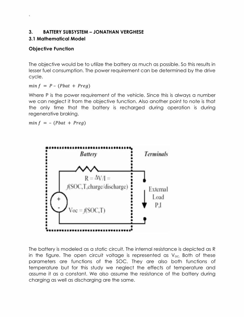
The battery is modeled as a static circuit. The internal resistance is depicted as R
in the figure. The open circuit voltage is represented as Voc. Both of these
parameters are functions of the SOC. They are also both functions of
temperature but for this study we neglect the effects of temperature and
assume it as a constant. We also assume the resistance of the battery during
charging as well as discharging are the same.

`
We can write the power generated in a single cell with the formula.
When we solve for the roots of this equation we get
√
√
Discharge rate of the battery is given by
Also as previously mentioned
Both are functions of SOC. These parameters can be found out using curve
fitting to experimental data for a 9v Prius NiMh battery cell. This consists of cells in
parallel, , which are together called a module and many modules are
connected in series. Cells in parallel determine the current requirement of the
pack and cells in series determine the voltage requirement.
Adapting the results of curve fitting from a previous project.
Assumptions
The are considered as functions of SOC and the temperature
effect are not taken into consideration.
The charging and discharging resistances are assumed to be equal.
During operation the only way the battery is charged is by regenerative
braking. This is because of the architecture of the hybrid powertrain.
`
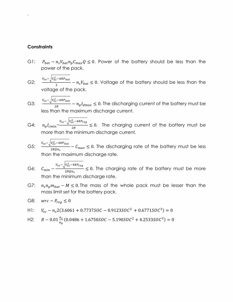
Constraints
G1: . Power of the battery should be less than the
power of the pack.
G2: √
. Voltage of the battery should be less than the
voltage of the pack.
G3: √
The discharging current of the battery must be
less than the maximum discharge current.
G4: − √
The charging current of the battery must be
more than the minimum discharge current.
G5: √
The discharging rate of the battery must be less
than the maximum discharge rate.
G6: √
The charging rate of the battery must be more
than the minimum discharge rate.
G7: The mass of the whole pack must be lesser than the
mass limit set for the battery pack.
G8:
H1:
H2:

`
Design Variables
- Number of cells in series
- Number of cells in parallel
- Power generated by the battery
- Power generated by regenerative braking
Design Parameters
- Minimum SOC
- Maximum SOC
- Mass of each cell
- Mass of the entire battery
- Open Circuit voltage
- Battery internal resistance
- Battery Capacity
- Nominal Cell voltage
- Maximum discharge rate of the cell
- Minimum discharge rate of the cell
- Maximum discharge current
- Minimum charging current
- Weight factor
The initial mathematical model prepared in the project proposal and the
progress report contained a few more constraints that were removed to
simplify the model. In the project proposal it was planned to conduct an
optimization study in two different fronts i.e. the pack level design and the
cell level design. The cell level design was to consider factors like anode and
cathode thickness, its porosity and number of layers. The objective function
that the problem was designed to minimize the volume of the cell. At the
pack level design the objective was to minimize the weight by varying the
module sizes depending upon requirements of the driving cycle. This problem
was changed to the current status as it had more relevance to the other

`
subsystems and the overall optimization of the system. The changing of the
objective to maximize the power generated by the

`
3.2 Model Analysis
Function Dependency Table
These functional dependency tables shows the relationship between the
variables and parameters with respect to the objective function and the
constraints.
1. With Variables
* *
G1 * * *
G2 * *
G3 * *
G4 * *
G5 * *
G6 * * *
G7 * *
G8 *
2. With Parameters
G1 * * *
G2 * * *
G3 * * *
G4 * * *
G5 * * * *
G6 * * * *
G7 * *
G8

`
Monotonicity Analysis
G1
G2
G3
G4
G5
G6
G7
G8
From the monotonicity analysis it seems that the problem seems well bounded.
According to MP1 every increasing variable must bounded below by a non-
increasing active constraint and every decreasing variable must be bounded
above by an increasing active constraint. In this case G1 is active for . G8 will
be active with respect to According to MP2 nonobjective variables should
be bounded from above and below by semi-active constraints and in this case
and are the nonobjective variables and they are bounded below and
above. These results could be validated with the help fmincon solver to observe
the activity of the constraints.
`
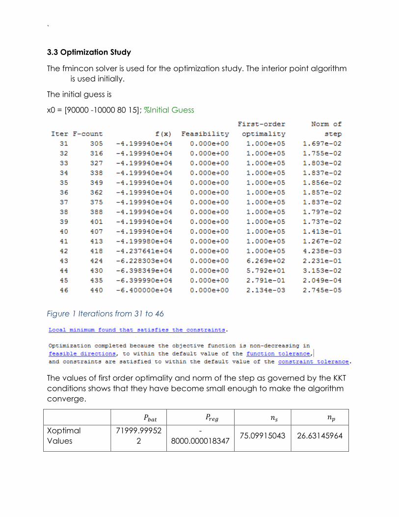
3.3 Optimization Study
The fmincon solver is used for the optimization study. The interior point algorithm
is used initially.
The initial guess is
x0 = [90000 -10000 80 15]; %Initial Guess
Figure 1 Iterations from 31 to 46
The values of first order optimality and norm of the step as governed by the KKT
conditions shows that they have become small enough to make the algorithm
converge.
Xoptimal
Values
71999.99952
2
-
8000.000018347 75.09915043 26.63145964

`
These are the optimal values obtained from fmincon. The power generated
calculated comes up to 72kW.
Figure 2 Plot for Function value with the iterations using the interior point
algorithm
Lagrange Multipliers At Lower Bound At Upper Bound
1.36770609803501e-05 0.000110438217930799
7.19755819592180e-06 5.75971242691069e-06
6.11699375500355e-06 0.000467108191695625
3.82739646333024e-06 0.00145627272933446
This table shows the Lagrange multipliers at the upper and lower bounds. All of
them are zero that means that none of the constraints are active.

`
Below are the values of the hessian at the optimal solution
0.000410 0.002307 0.053238 0.062735
0.002307 0.497961 0.019243 0.026689
0.053238 0.019243 75.50823 123.8445
0.062735 0.026689 123.8445 204.7913
As it can be seen, the hessian is positive definite that shows convexity of the
objective function in the constrained space.
Change in Design variables with change in the initial guess
Starting Point 1 Starting Point 2 Starting Point 3
75 67 73
27 30 28
72kW 72kW 72kW
8kW 8kW 8kW
This table shows how the design variables change with the change in starting
point. The values of the power from the battery and power obtained during
regeneration always converge to the same values but the values of number of
cells in series and parallel change.
This optimization problem was run using a few other algorithms to check validity
of results obtained and to provide a comparison between the different
algorithms to see the efficiency of each of them.
`
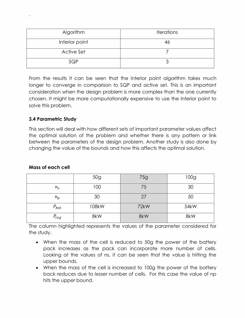
Algorithm Iterations
Interior point 46
Active Set 7
SQP 3
From the results it can be seen that the interior point algorithm takes much
longer to converge in comparison to SQP and active set. This is an important
consideration when the design problem is more complex than the one currently
chosen. It might be more computationally expensive to use the interior point to
solve this problem.
3.4 Parametric Study
This section will deal with how different sets of important parameter values affect
the optimal solution of the problem and whether there is any pattern or link
between the parameters of the design problem. Another study is also done by
changing the value of the bounds and how this affects the optimal solution.
Mass of each cell
50g 75g 100g
100 75 30
30 27 50
108kW 72kW 54kW
8kW 8kW 8kW
The column highlighted represents the values of the parameter considered for
the study.
When the mass of the cell is reduced to 50g the power of the battery
pack increases as the pack can incorporate more number of cells.
Looking at the values of ns, it can be seen that the value is hitting the
upper bounds.
When the mass of the cell is increased to 100g the power of the battery
back reduces due to lesser number of cells. For this case the value of np
hits the upper bound.

`
In one case the voltage of the battery is constrained and in another case the
capacity is constrained, as the number of cells in series affects the voltage of
the battery and the number of cells in parallel affect the battery capacity.
Mass of the battery pack
100kg 150kg 250kg
85* 75 100
13* 27 30
50kW* 72kW 110kW
8.1kW* 8kW 8kW
The column highlighted represents the values of the parameter considered for
the study.
For the case when the mass of the battery pack is 100kg the solution does
not converge.
For the case when the mass of the battery pack is 250kg the ns value hits
the upper bounds because more number of cells can be added and so
the voltage increases and therefore the power produced by the pack
increases.
Voltage of each cell
6V 7.2V 9V
67 75 97
30 27 21
60kW 72kW 83kW
8kW 8kW 8kW
The column highlighted represents the values of the parameter considered for
the study.
Understandably for the case when the voltage is 6V the power of the
pack has reduced.

`
For the case when the cell voltage is 9V a higher value of power is seen.
The number of cells have also increased leading to an increase in the max
operating voltage.
Capacity of each cell
3.3A-h 5A-h 10A-h
67* 75 100
30* 27 12
50kW* 72kW 50kW
8kW* 8kW 8kW
The column highlighted represents the values of the parameter considered for
the study.
For the case when the capacity of the cell is 3.3A-h the solution does not
converge.
When the capacity of the cell is 10A-h the ns value hits the upper bound.
The interesting observation in this parametric study is that unlike the other
studies power of the battery pack does not vary linearly with change in
capacity.
Varying the bounds of the
Trial 1 Trial 2 Trial 3
75 85 87*
27 24 23*
72kW 72kW 75kW*
8kW 8kW 8kW*

`
The column highlighted represents the values of the bounds considered for the
study.
Trial 1: lb = [50000 -12000 50 10]; %Lower bound of decision variables
ub = [150000 -3000 100 30]; %Upper bound of decision variables
Trial 2: lb = [25000 -12000 50 10]; %Lower bound of decision variables
ub = [250000 -3000 100 30]; %Upper bound of decision variables
Trial 3: lb = [75000 -12000 50 10]; %Lower bound of decision variables
ub = [100000 -3000 100 30]; %Upper bound of decision variables
In all the cases the remains almost the same but the values of and
change therefore affecting the values of max operating voltage and battery
capacity.
Varying the bounds of and
Trial 1 Trial 2 Trial 3
75 65 80
27 31 25
72kW 72kW 72kW
8kW 8kW 8kW
The column highlighted represents the values of the bounds considered for the
study.
Trial 1: lb = [50000 -12000 50 10]; %Lower bound of decision variables
ub = [150000 -3000 100 30]; %Upper bound of decision variables
Trial 2: lb = [50000 -12000 50 10]; %Lower bound of decision variables
ub = [150000 -3000 150 50]; %Upper bound of decision variables
Trial 3: lb = [50000 -12000 50 10]; %Lower bound of decision variables
ub = [150000 -3000 80 25]; %Upper bound of decision variables
In all the cases the remains the same but the values of and change
therefore affecting the values of max operating voltage and battery capacity.
What’s interesting is even after relaxing the bounds on the value decreases
and not increases but the value of on the other hand increases. The last case
as expected when the bounds were made tighter for the values hit the
upper bounds.
`
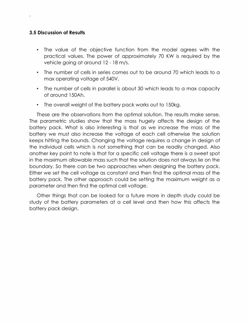
3.5 Discussion of Results
• The value of the objective function from the model agrees with the
practical values. The power of approximately 70 KW is required by the
vehicle going at around 12 - 18 m/s.
• The number of cells in series comes out to be around 70 which leads to a
max operating voltage of 540V.
• The number of cells in parallel is about 30 which leads to a max capacity
of around 150Ah.
• The overall weight of the battery pack works out to 150kg.
These are the observations from the optimal solution. The results make sense.
The parametric studies show that the mass hugely affects the design of the
battery pack. What is also interesting is that as we increase the mass of the
battery we must also increase the voltage of each cell otherwise the solution
keeps hitting the bounds. Changing the voltage requires a change in design of
the individual cells which is not something that can be readily changed. Also
another key point to note is that for a specific cell voltage there is a sweet spot
in the maximum allowable mass such that the solution does not always lie on the
boundary. So there can be two approaches when designing the battery pack.
Either we set the cell voltage as constant and then find the optimal mass of the
battery pack. The other approach could be setting the maximum weight as a
parameter and then find the optimal cell voltage.
Other things that can be looked for a future more in depth study could be
study of the battery parameters at a cell level and then how this affects the
battery pack design.

`
4. MECHANICAL COUPLER SUBSYSTEM – KARAN SHAH
4.1 MATHEMATICAL MODEL
OBJECTIVE FUNCTION
To minimize the weight of the mechanical coupler that transmits the maximum
power and the maximum torque to meet the demands of the Hybrid Electric Bus
which directly affects the fuel economy of the Hybrid Electric Bus based on the
urban driving conditions for a city bus.
Minimize W =
W.r.t b, r, G
Where,
W = Weight of the mechanical coupler, Kg
r = Pitch Radius of the input gear of the mechanical coupler, mm
b = Width of the gear teeth, mm
ρ = Density of the material used for the input and output gears, Kg/mm3
G = Gear ratio between the input gears and the output gear of the mechanical
coupler, dimensionless
Since, the weight of the mechanical coupler directly impacts the weight of the
vehicle which effectively affects the torque and speed demands of the vehicle.
The torques produced by the motor and the engine are coupled by the
mechanical coupler which results in a multiplied torque output due to the gear
ratio of the mechanical coupler. The fuel rate consumption can be determined
by the weight of the vehicle as per the speed and torque demands. Thus, the
fuel consumption can be calculated for a given weight of the mechanical
coupler and the optimized fuel efficiency can be obtained from the minimized
weight of the coupler.
CONSTRAINTS
1. The bending stress induced on the teeth of the input gear during meshing
should be lesser than or equal to the maximum allowable bending stress of the
material of the gears.
σbi ≤ σbmax
i.e. σbmax - σbi ≤ 0

`
2. The bending stress induced on the teeth of the output gear during
meshing should be lesser than or equal to the maximum allowable bending
stress of the material of the gears.
σbo ≤ σbmax
i.e. σbmax - σbo ≤ 0
3. The Contact Surface stress induced on the teeth of the input and output
gear during meshing should be lesser than or equal to the maximum endurance
limit of the material of the gears.
σcgt ≤ σendl
σcgt - σendl ≤ 0
√ ( √ √ )
√ √ √
4. The radii of the input gears of the mechanical coupler cannot be lesser
than or equal to zero.
r > 0
-r < 0
5. The Width of the teeth of the input gears and the output gear of the
mechanical coupler cannot be lesser than or equal to zero.
b > 0
-b < 0
6. The Gear ratio between the input gears and the output gear of the
mechanical coupler cannot be lesser than or equal to zero.
G > 1
G – 1 > 0
-G + 1 < 0
7. The design constraint, which is the ratio of the Width of the gear to its
radius is equal to the ratio of gear ratio to the sum of gear ratio and 1.
b/r = G/G + 1
b*(G + 1) – r*(G) = 0

`
DESIGN VARIABLES & PARAMETERS
Design Variables:
Radii of the input gears, r
Width of the gear, b
Gear Ratio between the gear train, G
Module of the gear, m (Usually, the value of m = 1)
Parameters:
Input Torque to the input gears, T
Maximum bending stress induced on the gear teeth, σbi, σbo
Maximum contact surface stress induced on the gear teeth, σcgt
Acceleration of the hybrid electric bus, a
Pressure angle, Φ
Module of the spur gears, m
Young’s Modulus of the gear material, E
Poisson’s Ratio of the gear material, μ
SUMMARY MODEL
Minimize the f(x) = Weight of the Mechanical Coupler, (W) of the Mechanical
Coupler, of a Hybrid Electric Bus under urban city driving conditions.
Minimize f(x) =
W.r.t. r, b, G
Subject to
G1
G2
G3 √ ( √ √ )
( ) √ √ √
G4 -r < 0
G5 -b < 0
G6 -G + 1 < 0
G7 b*(G + 1) – r*(G) = 0

`
EVOLUTION OF THE PROBLEM AND LIST OF ASSUMPTIONS
1. The optimization problem is formulated for minimization of weight of the
mechanical coupler transmission system for the hybrid electric bus. The
constraints are directly dependent on the input torque provided to the coupler.
Initially, the torque was taken as the maximum value demanded by the vehicle.
Over the span of the project, it was realized that the torque values varies and is
dependent on the acceleration of the vehicle. This was the major evolution that
occurred in the problem formulation of the optimization project.
2. The values for ρ, σbmax & σcmax will be obtained from standard mechanical
and material properties for the chosen material for the design of the gear train
of the mechanical coupler.
3. The values for m, Φ will be determined based on the type and size of the
final gears selected for the gear train of the mechanical coupler.
4. The geometry of the Spur Gears design is considered to be cylindrical for
ease of weight and volume calculations.
5. The gears are involute and cycloidal in geometry.
6. The pressure angle (Φ) of the gears is taken as 20°.
7. Module of the spur gears (m) is taken as 1 mm.
8. The thickness of the gear is assumed to be equal to the face width of the
gear teeth.
9. The thickness or the width (b) of the gears is taken as equal for both input
and output gears.
10. The material used for the gears is 4130 Chrome Moly Steel.
i. Material Properties of 4130 Chrome Moly Steel are as follows:
ii. Ultimate Tensile Strength ( = 620 N/mm2
iii. Endurance Limit (σendl) = 480 N/mm2
iv. Young’s Modulus (E) = 200000 N/mm2
v. Density (ρ) = 0.78 x 10⁻⁵ Kg/mm3
11. Both the input gears are identical in dimensions.
12. Both the input gears are running at identical RPM when operated
together.
13. Friction losses, heat losses, energy losses and the efficiency of the
transmission are neglected during the optimization process.
`
4.2 MODEL ANALYSIS
The mathematical model formulated to carry out the optimization of the
mechanical coupler of the Hybrid Electric Bus yields the following results on the
basis of monotonicity analysis.
The objective function f(x) = is monotonic with
respect to the design variables R, b, G.
The monotonicity table (refer to the appendix to view the monotonicity
analysis) obtained by applying the monotonicity principles to the objective
functions f(x) and also to the corresponding constraints of this optimization
mathematical model.
The monotonicity analysis of the mathematical model of the optimization
problem also shows that the problem is well constrained subjected to a number
of constraints.
The design variable r shows that it is an increasing function and is
constrained from the bottom. Therefore, the variable moves upwards in the
positive direction to obtain its optimal value.
The design variable b shows that it is an increasing function and is
constrained from the bottom. Therefore, the variable moves upwards in the
positive direction to obtain its optimal value.
The design variable G however, shows that it is a decreasing function and
is constrained from the above therefore, the variable moves downwards in the
negative direction to obtain its optimal value.
The objective functions and the constraints are bounded optimization problems
and since they are linear equations of first order, they are monotonic in nature
with respect to the design variables. The various assumptions as discussed in the
previous section of the report like, the shape, geometry and the profile of the
gears, the material properties, the maximum torque, the pressure angle were
substituted into the various formulae to simplify the constraint equations in order
to carry out the iterations of the optimization problem cost efficiently.
All the dimensions of the various parameters and variables used in the
optimization problem were manually scaled into a uniform system of units and
therefore, no scaling functions were used to scale the objective function and
the constraints.
The variables and parameters are all converted and scaled into the following
set of uniform dimension system based on the category they belong. Length,

`
mm; Weight, Kg; Stresses/Strengths, N/mm2; Density, Kg/mm3; Acceleration,
mm/s2
4.3 OPTIMIZATION STUDY
The following section of the report focusses on the optimization method used to
minimize the weight of the mechanical coupler and the results obtained from
the optimization problem.
The optimization problem has one objective function with three inequality
constraints and one equality constraint like explained earlier in this report. This
indicates that this is a constrained optimization problem with non-linear
constraints. Therefore, the optimization is carried out by the Optimization toolbox
in MATLAB using the ‘FMINCON – Constrained nonlinear minimization’ solver.
The ‘FMINCON’ solver uses 4 types of algorithms to carry out the optimization
process which are namely, Interior Point, SQP, Active Set, Trust Region Reflective
algorithms. The results obtained using these four algorithms will be compared to
find the optimized solution for the design variables which will in turn yield the
optimal weight of the mechanical coupler of the hybrid electric vehicle.
The optimization is carried out for three different starting points. Refer to the
appendix of this report to view the various plots and results for the design
variables and the weight of the coupler. The final results and a further analysis of
the results obtained are explained precisely below.
Radii of the input gears, r = 75 mm
Radius of the output gear, R = 150 mm
Width of the input gears, b = 45 mm
Gear Ratio of the mechanical coupler = 1.6
Weight of the mechanical coupler = 27.46 Kg
Command Window Output from MATLAB:
Diagnostic Information (Output using Optimization Toolbox)
Number of variables: 3
Functions
Objective: PROJFUN (See appendix for the objective function code)
Gradient: finite-differencing
Hessian: finite-differencing (or Quasi-Newton)

`
Nonlinear constraints: PROJNONLCON (See appendix for the Nonlinear
constraints code)
Nonlinear constraints gradient: finite-differencing
Constraints
Number of nonlinear inequality constraints: 3
Number of nonlinear equality constraints: 1
Number of linear inequality constraints: 0
Number of linear equality constraints: 0
Number of lower bound constraints: 0
Number of upper bound constraints: 0
Algorithm selected
Sequential quadratic programming
____________________________________________________________
End diagnostic information
Optimization completed: The relative first-order optimality measure, 6.290114e-
08,
is less than options.TolFun = 1.000000e-06, and the relative maximum constraint
violation, 2.000687e-14, is less than options.TolCon = 1.000000e-06.
Optimization Metric Options
relative first-order optimality = 6.29e-08 TolFun = 1e-06 (default)
relative max(constraint violation) = 2.00e-14 TolCon = 1e-06 (default)
OUTPUT USING THE ‘FMINCON’ SOLVER CODE
Local minimum found that satisfies the constraints.
Optimization completed because the objective function is non-decreasing in
feasible directions, to within the default value of the function tolerance, and
constraints are satisfied to within the default value of the constraint tolerance.
<stopping criteria details>
Active inequalities (to within options.TolCon = 1e-06):
lower upper ineqlin ineqnonlin

`
3
xopt =
45.4387 74.5094 1.5630
fval =
27.4648
exitflag =
1
output =
iterations: 9
funcCount: 40
lssteplength: 1
stepsize: 1.0177e-04
algorithm: 'medium-scale: SQP, Quasi-Newton, line-search'
firstorderopt: 6.8581e-07
constrviolation: 1.2810e-09
message: [1x783 char]
lambda =
lower: [3x1 double]
upper: [3x1 double]
eqlin: [0x1 double]
eqnonlin: 1.7423e-07
ineqlin: [0x1 double]
ineqnonlin: [3x1 double]
grad =
0.6044
0.7372
19.3237
hessian =
0.0234 0.0233 0.6550
0.0233 0.0299 0.7729
0.6550 0.7729 29.6534
`
ANALYSIS OF RESULTS
The results provided above explicitly explains various aspects of the optimization
process.
The third inequality constraint is active for this optimization problem which
is also justified from the monotonicity analysis of the optimization problem.
Therefore, since the constraint is active, there exists a positive Lagrange
multiplier as per the rules of nonlinear constrained optimization.
The value of the Lagrange multiplier is obtained as 1.7423e-07.
The results explains that the optimization completed as local minimum was
found which satisfies the constraints. Also, The relative first-order optimality
measure, 6.290114e-08, is less than options.TolFun = 1.000000e-06, and the
relative maximum constraint violation, 2.000687e-14, is less than options.TolCon =
1.000000e-06. This indicates that the results are numerically stable and within the
tolerance limits.
The same results are obtained when the Active Set Algorithm is used for
the optimization problem. Refer to the appendix of this report to view these
results. As per MATLAB, Active Set algorithm is based on the KKT conditions.
Since, the optimization completed as the local solution is found that satisfies the
constraints and is also within the tolerance limits. Therefore, it can be concluded
that the optimum solution is obtained that satisfies the KKT solutions.
The optimization is carried out by taking into consideration three different
starting point. For all the starting point combined with the various algorithms to
solve the optimization problem, the values for the design variables converge at
the same point which is the global optimal solution for the optimization problem.
Refer to the appendix of this report to view all the results.
The monotonicity results agrees with the numerical values obtained from
the result obtained. Both the design variables, i.e. the radii (r) and the width (b)
of the input gears are monotonically increasing variables while the gear ratio of
the coupler is monotonically decreasing function.
4.4 PARAMETRIC STUDY
The optimization model’s parametric study can be carried for the set of
parameters like material properties and acceleration of the hybrid electric bus
and the gear design parameters is explained below in the form of comparison
study between two different sets pf parameter values. The optimization is carried

`
out using the SQP Algorithm which is an efficient algorithm with a starting point
[1000 1000 10]
For a fixed set of parameters like:
i. Material = Grey Cast Iron; E = 160 GPa; Ultimate tensile Strength = 430 MPa;
Endurance Limit = 170 MPa, Density = 0.72 Kg/mm
Results obtained:
b = 84 mm; r = 137 mm; G = 2.4; W = 157 Kg;
Plot:
ii. Material = Carbon Steel; E = 190 GPa; Ultimate tensile Strength = 550 MPa;
Endurance Limit = 340 MPa, Density = 0.78 Kg/mm
Results Obtained:
b = 57; r = 91; G = 1.9; W = 51 Kg;

`
Plot:
iii. Material = 4130 Chome Moly Steel; E = 206 GPa; Ultimate tensile Strength =
620 MPa;
Endurance Limit = 480 MPa, Density = 0.78 Kg/mm
Results Obtained:
b = 45 mm; r = 75 mm; G = 1.6; W = 27.46 Kg;
Plot:
The iterations while carrying out the optimization for the weight of the
mechanical coupler showed the following trend. As the material properties
parameters increased in numerical value for the ultimate tensile strength,

`
Endurance limit and Young’s Modulus, the dimensions of the design variables
like radii and width of the input gear decreased however, the gear ratio of the
coupler also reduced. Therefore, this shows that there is a tradeoff between the
gear ratio and the dimensions of the input gears. The Weight of the coupler also
reduced as the material properties increased in the numerical value.
In simple words, the weight obtained when grey cast iron was used as a material
was the maximum in comparison to the weight obtained when carbon steel was
used as the material. The weight further reduced when the material used was
4130 Chrome Moly steel which has been used as the gear material for this
optimization project.
Therefore, the results can be generalized as the material which has the greater
Ultimate Tensile Strength, Endurance Limit and Young’s Modulus will have the
lowest weight when used as the gear material for the mechanical coupler.
The ranges for the parameters obtained from the above results are the
following:
Ultimate Tensile Strength range: 430 MPa – 1100 MPa
Endurance Limit range: 170 MPa – 550 MPa
Young’s Modulus range: 160 GPa – 210 GPa
Weight Range: 160 Kg – 16 Kg
Gear Ratio Range: 2.6 – 0.7
Note: A gear ratio lesser than 1 is not acceptable as the purpose of the
mechanical torque coupler is lost, as the output torque from the mechanical
torque coupler will be lower than the input torque provided to the coupler.
4.5 DISCUSSION OF RESULTS
The design implications that can be observed from the above obtained
results based on constrained optimization as well as parametric study is that, the
weight of the coupler is reduced as the material used for manufacturing the
spur gears has greater material and mechanical properties, i.e. weight of the
coupler is inversely proportional to the strength, toughness and elasticity of the
material.
The design rule identified from the solutions obtained is the for having an
optimum weight for a mechanical torque coupler, the ideal gear ratio between
the gear train should be in the range of 1.5 – 2.0. This implies that the output
gear of the coupler should have number of teeth and its pitch radius 1.5 - 2.0

`
times the number of teeth and the pitch radius of the input gear respectively.
Also, another identified rule as discussed in the previous implication is that
weight decreases as the material becomes stronger and tougher.
The results do make sense as the dimensions and the weight obtained can
be easily comparable to the existing gear trains that are manufactured for the
commercial hybrid electric buses.
The model limits the solutions as the constraints are to be satisfied since the
optimization problem is constrained optimization. Therefore, the solution to the
optimization model can be obtained only in the range of points that satisfy all
the constraints and provide the minimized weight for the mechanical coupler.

`
5. OPTIMAL CONTROL SUBSYSTEM – GOVIND V MENON / SHANKER KRISHNAN
5.1 MATHEMATICAL MODEL
OBJECTIVE
Optimal control subsystem controls what to use when. It determines whether the
bus should be powered by the engine or the motor at any given time interval in
the EPA drive cycle. The main aim of this subsystem is to integrate the other
systems which the optimal control and provide an optimum values of mpg by
incorporating the ECMS algorithm and Pareto curves
CONSTRAINTS
The main constraints involved in the optimal control are the Torque limits
of the motor and the engine. This is calculated by basically selecting the motor
and the engine and then generating torque limit curves.
The motor that was used was basically an I-SAM motor. The top torque
limits of the motor were determined from a speed of 650 rpm to 2700 rpm. The
remaining values of the torque limit was interpolated linearly to get the values of
the torque limit for ‘’W’’ ranging from 0-3300 rpm.
The values of Ns and Np are limited by the battery constraints which also
contribute to the weight (Kerb weight)
Td = Tm+ Te
(Total torque demand is equal to the torque of engine + torque of the motor)
Te min <= Te <= Te max
(Torque of the engine must lie between the maximum and minimum value)
Tm min<= Tm <= Tm max
(Torque of the motor must lie between the maximum and the minimum value)
e min <= e <= e max
(The angular velocity of the engine must lie between the maximum and the
minimum value)

`
m min <= e <= e max
(The angular velocity of motor must lie between the maximum and the minimum
value)
5 < F.R < 15
(The values of the final drive ratio is limited in the ration of 8-15)
15< Ns < 50 and 10 < Np < 30
ASSUMPTIONS
Some of the assumptions that were made in the optimal control algorithm are as
follows
It is assumed that the bus follows the exact EPA cycle and does not
deviate from it at all times
The SOC of the battery is set to a value of 60% at the beginning and at the
end
It is assumed that the bus is operating at a constant Kerb weight.
We assume the ideal case of the engine where we are not including the
efficiency of the engine. This basically means that we are not considering the
various factors like friction, fuel quality etc.
The values of the EPA drive cycle are set for a particular urban bus in
orange county and may not be the same elsewhere
The linear interpolation made during the various segments of the program
which may not be actually true in practical cases
The motor efficiency meaning is always taken as 95% of the calculated
efficiency
DESIGN VARIABLES AND PARAMETERS
The main design variables that are used are
1. m (rpm)
2. e (rpm)
3. Tm (Nm)
4. Te (Nm)
5. Td (Nm)
6. Ns , Np

`
DESIGN PARAMETERS
1. Final drive ratio ( FR )
2. Maximum Engine torque (Te max ) – 800 Nm
3. Maximum Engine angular velocity ( e max ) -1600 rpm
4. Maximum Motor output – 120 Kw – VOLVO I SAM electric motor
5. Motor Torque range ( Tm ) – 800/1200 Nm
5.2 MODEL ANALYSIS
Since the subsystem mainly deals with the programing part it does not have a
mathematical formula to indicate its working pattern
The main objective of the optimal control is to use the ECMS algorithm to
determine the maximum fuel efficiency and at the same time conserving the
battery use
Optimization is done by creating grids of look up tables of the fuel
efficiency and the power of the battery which are used to obtain the values of
the drive mode characteristics at a certain point
The maximum current consumed by the motor is set between two bounds
to prevent infeasible mode/operating points to appear in the look up table
The values of optimum point is developed using the equation
EC = Fuel + λ*Power of battery
The value of lambda is calculated using a simple root finding algorithm to
determine whether the SOC reaches the required values at the end of the
cycle.
5.3 BASIC FLOW OF THE PROGRAM
The optimal control subsystem is made up of various sub modules that
determine the characteristics of the engine and the motor at a particular time.
Based on these operating conditions the optimum mode is selected using the
`
ECMS algorithm. The main sub modules that are being considered for the
project are
1. Engine control
2. Motor control
3. Transmission control
4. Battery power control
Optimal control is centrally controlled by a main program which reads the
values from the EPA drive cycle and computes the values of the torque and the
speed required by the bus. This program requires the following inputs
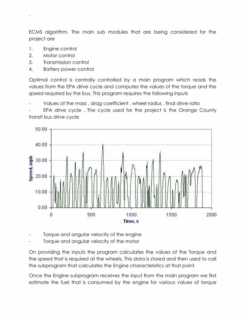
- Values of the mass , drag coefficient , wheel radius , final drive ratio
- EPA drive cycle . The cycle used for the project is the Orange County
transit bus drive cycle
- Torque and angular velocity of the engine
- Torque and angular velocity of the motor
On providing the inputs the program calculates the values of the Torque and
the speed that is required at the wheels. This data is stored and then used to call
the subprogram that calculates the Engine characteristics at that point.
Once the Engine subprogram receives the input from the main program we first
estimate the fuel that is consumed by the engine for various values of torque

`
and angular velocity. These values of the fuel consumption are stored in a grid
which is used as a look up grid later. On calculating the engine torque we can
understand the deficient torque which is required to power the bus at that point
of time.
This deficiency of the torque ids satisfied by the motor. The motor program is
used for this purpose. It calculates the amount of torque provided by the motor
and estimates the current that is required or used up by the motor at that point.
This value of current is used to determine the battery requirement and this leads
us to a Battery power grid.
Thus after running these subprograms we now have a grid f fuel consumption
and power of battery. These grids are used to create a Pareto curve. A Pareto
curve uses a Pareto front, what this does is that it helps making tradeoffs and
selecting the most feasible points among all the sets of points so that we do not
have to go through the entire grid.
Along with these subprograms there is a section of coding in the optimal control
that helps in the regenerative braking. This is based on the fact that every
downfall of the EPA drive cycle curve denotes a point where the brake is
applied or when the bus is decelerating. At these points the energy from the
motion is used to recharge the battery using a simple motor that acts as a
generator. This helps in improving the charge in the battery.
After we generate the Pareto curves for the entire drive cycle we perform the
ECMS on these points. The ECMS algorithm helps in selecting the optimum mode
that is required at each time step of the operation of the bus so that maximum
fuel efficiency is attained and at the same time the battery holds enough
charge. This is done based on the SOC values which are taken into
consideration while calculating the Equivalent consumption
`
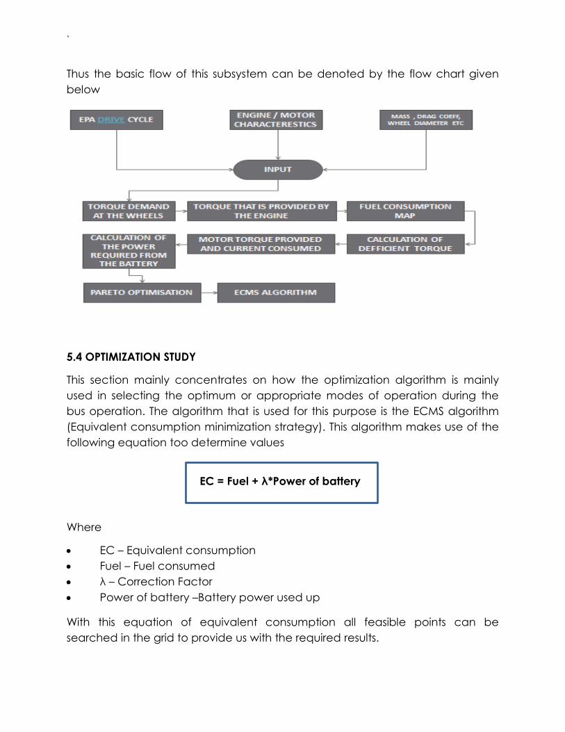
Thus the basic flow of this subsystem can be denoted by the flow chart given
below
5.4 OPTIMIZATION STUDY
This section mainly concentrates on how the optimization algorithm is mainly
used in selecting the optimum or appropriate modes of operation during the
bus operation. The algorithm that is used for this purpose is the ECMS algorithm
(Equivalent consumption minimization strategy). This algorithm makes use of the
following equation too determine values
EC = Fuel + λ*Power of battery
Where
EC – Equivalent consumption
Fuel – Fuel consumed
λ – Correction Factor
Power of battery –Battery power used up
With this equation of equivalent consumption all feasible points can be
searched in the grid to provide us with the required results.

`
During the drive cycle the values of the Equivalent consumption can be
calculated by using the fuel consumption and the batter power. At any
particular time the characteristics of the engine and the motor are determined
by minimizing the equivalent consumption and comparing those values with the
Pareto curves that provide us with the lookup tables.
The value of the correction factor λ is chosen based on the values of the SOC.
The correction factor λ chosen s considered to be correct if
|SOCi-SOCf |= 0 (within some tolerance)
The SOC values that are chosen for the this project are at 60% the values of
lambda are then calculated by a simple root finding algorithm leading us
different values of lambda until the end SOC value is accurate within ±4%
accuracy .
This process is repeated for all the values of times steps and the modes for each
vehicle speed and torque are determined which together give us the optimum
fuel efficiency of the bus. When the values of any of the parameters like FR ,
engine motor characteristics etc. change it leads to generation of new set of
pareto curves after which the ECMS algorithm is performed again

`
5.5 DISCUSSION OF RESULTS
The optimal control subprogram finally gives us the mileage (mpg) of the bus for
the given drive cycle. Several runs performed were performed in the optimal
control which produced the SOC curves.
The graph above denotes the SOC curve. This run gave an mpg of 1.3411.
The graph also shows that the battery use has been very negligible (about 0.5%).
This is a result of the battery capacity being too high than what was required for
the operation of the bus

`
The above graph is for another run of the optimal control wherein the
battery usage has reached 10%. The corresponding mpg values obtained for
this run was close to 6.1348.
The graph shows that there is more optimal usage of the battery as well as
the engine for powering the bus
Based on multiple runs of the optimal control the mpg using the 3 systems
combined was coming in the range of 5-7 mpg. This is almost 80% more efficient
than a common transit bus which uses diesel engine alone

`
6. SYSTEM INTERGRATION STUDY
The main objective of system integration is to obtain a maximum mpg value that
is optimum after considering the results obtained from the individual subsystems
The system integration is done by taking in the values from the all the three
subsystems and finding the optimum values based on these three system. It is
done by using the fmincon function in matlab
The inputs to this fmincon function are the following
- Ns , Np values
- FR values
The value of Ns determines the voltage
The value of Np determine the battery capacity
FR value determines coupler mass
All the three values also contribute to the total mass of the system and thus
varying these values will change the mass of the bus which in turn will affect the
mpg values.
The results that were obtained from the individual subsystems were
From the battery subsystem we get the values of Ns and Np
- Ns=75
- Np=27
The value of FR value from the torque coupler
- FR = 8
- Mass of coupler = 27.46 kg
On running the final code of the optimal control along with the other subsystems
the following results have been obtained for the transit bus operating in the
Orange county drive cycle using a given engine and motor characteristics
`
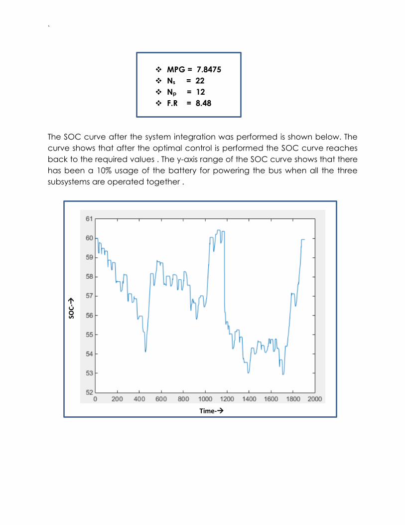
MPG = 7.8475
Ns = 22
Np = 12
F.R = 8.48
The SOC curve after the system integration was performed is shown below. The
curve shows that after the optimal control is performed the SOC curve reaches
back to the required values . The y-axis range of the SOC curve shows that there
has been a 10% usage of the battery for powering the bus when all the three
subsystems are operated together .
Time-
SOC
-

`
7. REFERENCES
BATTERY SUBSYSTEM
[1] Design and Optimization of Lithium-Ion Batteries for Electric-Vehicle
Applications by Nansi Xue, Wenbo Du, Thomas A. Greszler, Wei Shyy, Joaquim R.
R. A. Martins
[2] Modern Electric, Hybrid Electric, and Fuel Cell Vehicles: Fundamentals,
Theory, and Design, Second Edition by Mehrdad Ehsani, Yimin Gao, Ali Emadi.
[3] Overview Of Battery Models
http://www.thermoanalytics.com/docs/batteries.html
[4] Energy Management Strategy for a Parallel Hybrid Electric Truck Chan-Chiao
Lin, Jun-Mo Kang, J.W. Grizzle, and Huei Peng
[5] Optimal Design of Hybrid Electric Vehicle for Fuel Economy by Archit Ratogi
et al, University of Michigan, MEE 55-12-04
[6] Optimal Design of Hybrid Electric Vehicle by Shifang Li et al, University of
Michigan, MFG 555-2008-Winter
[7] Design of a Lithium-ion Battery Pack for PHEV using a Hybrid Optimization
method by Nansi Xue, Wenbo Du, Thomas A. Greszler, Wei Shyy, Joaquim R. R. A.
Martins, Ann Arbor, Michigan, USA
MECHANICAL COUPLER SUBSYSTEM
[1] A Textbook of Machine Design by R.S. Khurmi and J.K. Gupta.
[2] Practical Information on Gears by KOHARA GEAR INSTURY CO. LTD.
[3] Center Distance Minimization of A Single-Reduction, Single-Enveloping Worm
Gear Set; Ibrahim E. Cildir, University of Michigan,
[4] Design Optimization of the Spur Gear Set Anjali Gupta, U.I.E.T, Panjab
University Chandigarh, India.
[5] Spur Gear Optimization By Using Genetic Algorithm by Yallamti Murali
Mohan, T. Seshaiah, Department of Mechanical Engineering, QIS College of
Engineering Technology, Ongole, Andhra Pradesh
[6] Gear Tooth Strength Analysis by Dr. W.H. Dornfeld, Fairfield University
[7] Gear Design equations and formulae by Engineers Edgeinvolute Spur Gear
Design, IIT Madras, India

`
[8] ASM Aerospace Specification Metals Inc. for Material data about 4130
Chrome Moly Steel
http://asm.matweb.com/search/SpecificMaterial.asp?bassnum=m4130r
[9] MakeItFrom.com for material properties about Grey Cast Iron and Carbon
Steels
http://www.makeitfrom.com/
[10] The Engineering Toolbox website for material data, Ultimate tensile stress
and Endurance limit for various materials used in the project.
http://www.engineeringtoolbox.com/
OPTIMAL CONTROL SUBSYSTEM
[1] Design of hybrid-electric vehicle architectures using Auto-generation of
feasible driving modes by Alparslan Emrah Bayrak , Yi Ren , Panos Y.
Papalambros
[2] Equivalent fuel consumption optimal control of a series hybrid electric vehicle
by J-P Gao, G-M G Zhu, E G Strangas and F-C Sun
[3] Configuration Analysis for Power Split Hybrid Vehicles with Multiple Operating
Modes by Xiaowu Zhang Chiao-Ting Li Dongsuk Kum Huei Peng Jing Sun
[4] Modeling and Control of a Power-Split Hybrid Vehicle by Jinming Liu and Huei
Peng
`
8. APPENDICES
8.1 APPENDIX – A (BATTERY SUBSYSTEM)
MATLAB CODE
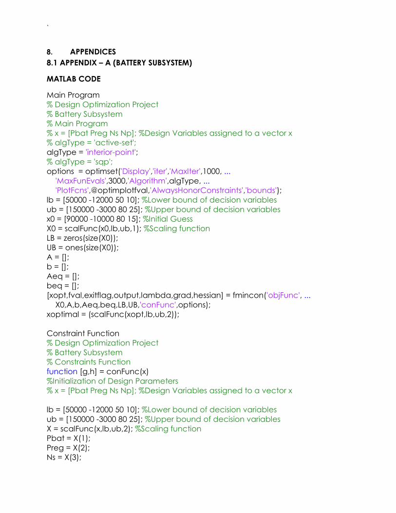
Main Program
% Design Optimization Project
% Battery Subsystem
% Main Program
% x = [Pbat Preg Ns Np]; %Design Variables assigned to a vector x
% algType = 'active-set';
algType = 'interior-point';
% algType = 'sqp';
options = optimset('Display','iter','MaxIter',1000, ...
'MaxFunEvals',3000,'Algorithm',algType, ...
'PlotFcns',@optimplotfval,'AlwaysHonorConstraints','bounds');
lb = [50000 -12000 50 10]; %Lower bound of decision variables
ub = [150000 -3000 80 25]; %Upper bound of decision variables
x0 = [90000 -10000 80 15]; %Initial Guess
X0 = scalFunc(x0,lb,ub,1); %Scaling function
LB = zeros(size(X0));
UB = ones(size(X0));
A = [];
b = [];
Aeq = [];
beq = [];
[xopt,fval,exitflag,output,lambda,grad,hessian] = fmincon('objFunc', ...
X0,A,b,Aeq,beq,LB,UB,'conFunc',options);
xoptimal = (scalFunc(xopt,lb,ub,2));
Constraint Function
% Design Optimization Project
% Battery Subsystem
% Constraints Function
function [g,h] = conFunc(x)
%Initialization of Design Parameters
% x = [Pbat Preg Ns Np]; %Design Variables assigned to a vector x
lb = [50000 -12000 50 10]; %Lower bound of decision variables
ub = [150000 -3000 80 25]; %Upper bound of decision variables
X = scalFunc(x,lb,ub,2); %Scaling function
Pbat = X(1);
Preg = X(2);
Ns = X(3);

`
Np = X(4);
Vbat = 7.2; %Nominal cell voltage
Cmax = 1; %Maximum cell discharge rate
Cmin = -1; %Minimum cell discharge rate
Icmin = -2; %Minimmum charging current
Idmax = 5.5; %Maximum discharge current
Q = 5; %Battery capacity
M = 150000; %Mass of the battery pack
mbat =75;
SOCmin = 0.3; %Minimum SOC fixed at 30%
SOCmax = 0.9; %Maximum SOC fixed at 90%
SOCrange = (SOCmin:0.1:SOCmax)';
% SOCrange = 0.3;
rc = -8000;
w = zeros(length(SOCrange),1);
w(SOCrange<=0.8) = 1;
id = (SOCrange>0.8&SOCrange<=0.9);
w(id) = 9-10*SOCrange(id);
Voc = Ns*2*(3.6061 + 0.7737*SOCrange - ...
0.9123*SOCrange.^2 + 0.6771*SOCrange.^3);
R = 0.01*(Ns/Np)*(0.0486 + 1.675*SOCrange ...
- 5.190*SOCrange.^2 + 4.2533*SOCrange.^2);
%Equality Contraints
h = [];
%Inequality Constraints
g = [Pbat - Ns*Vbat*Np*Cmax*Q ; (Voc - sqrt(Voc.^2 - 4*R*Pbat))/2 ...
- Ns*Vbat ; (Voc - sqrt(Voc.^2 - 4*R*Pbat))./(2*R) - Np*Idmax ; ...
Np*Icmin + (Voc - sqrt(Voc.^2 - 4*R*Preg))./(2*R) ; ...
(Voc - sqrt(Voc.^2 - 4*R*Pbat))./(2*R*Q*Ns) - Cmax ; Cmin - ...
(Voc - sqrt(Voc.^2 - 4*R*Preg))./(2*R*Q*Ns) ; Ns*Np*mbat - M ; ...
Preg - w*rc];
end
Objective Function
% Design Optimization Project
% Battery Subsystem
% Objective Function
function [f] = objFunc(x)
lb = [50000 -12000 50 10]; %Lower bound of decision variables
ub = [150000 -3000 80 25]; %Upper bound of decision variables
X = scalFunc(x,lb,ub,2); %Scaling function

`
f = -(X(1) + X(2)); %Objective function
end
Scaling Function
% Design Optimization Project
% Battery Subsystem
% Scaling Function
function X = scalFunc(x,l,u,type)
%This function scales the vector x that contains the design variables
%depending upon the bounds which are represente by l and u. Type is the
%flag variable where 1 is to scale and 2 is to unscale. This is done
%to maintain the vector of the same dimension
for i = 1:1:4
if type == 1
X(i) = (x(i) - l(i))/(u(i) - l(i));
else
X(i) = l(i) + x(i)*(u(i) - l(i));
end
end
Plots
Figure 3 Active Set Algorithm

`
Figure 4 SQP Algorithm
Figure 5 Curve Fitting for Voc wrt SOC

`
Figure 6 Curve Fitting for R wrt SOC
`
8.2 APPENDIX – B (MECHANICAL COUPLER SUBSYSTEM)
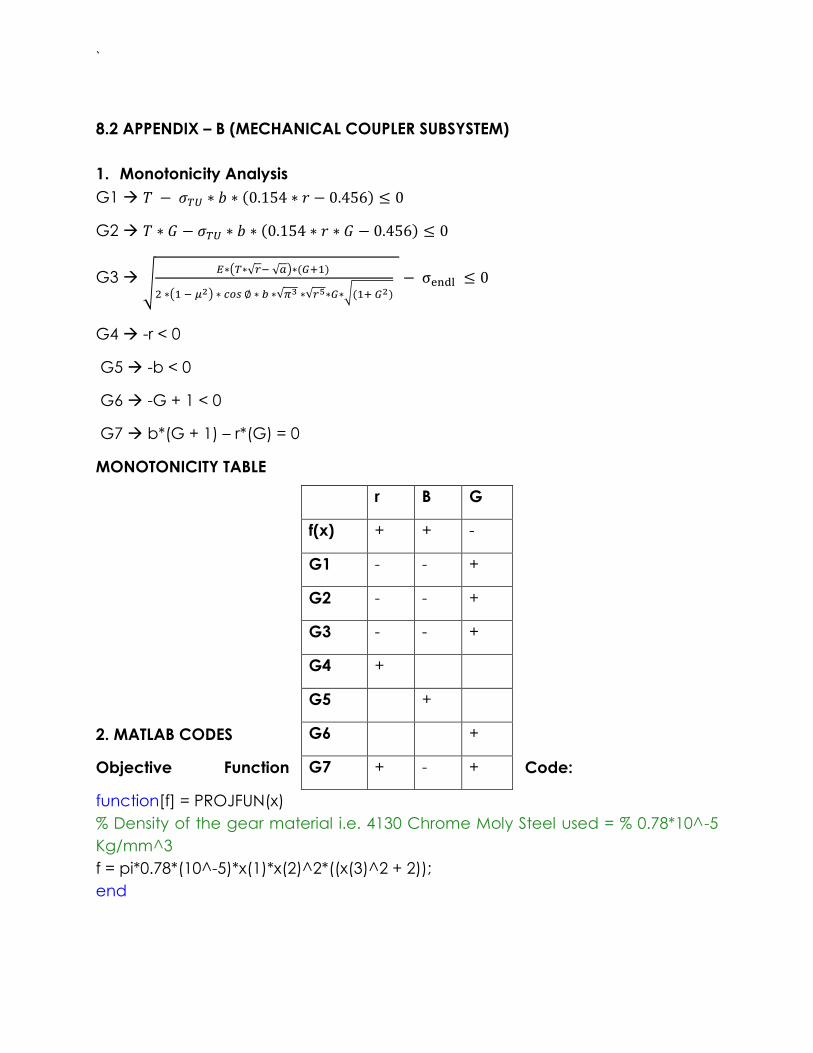
1. Monotonicity Analysis
G1
G2
G3 √ ( √ √ )
( ) √ √ √
G4 -r < 0
G5 -b < 0
G6 -G + 1 < 0
G7 b*(G + 1) – r*(G) = 0
MONOTONICITY TABLE
2. MATLAB CODES
Objective Function Code:
function[f] = PROJFUN(x)
% Density of the gear material i.e. 4130 Chrome Moly Steel used = % 0.78*10^-5
Kg/mm^3
f = pi*0.78*(10^-5)*x(1)*x(2)^2*((x(3)^2 + 2));
end
r B G
f(x) + + -
G1 - - +
G2 - - +
G3 - - +
G4 +
G5 +
G6 +
G7 + - +
`
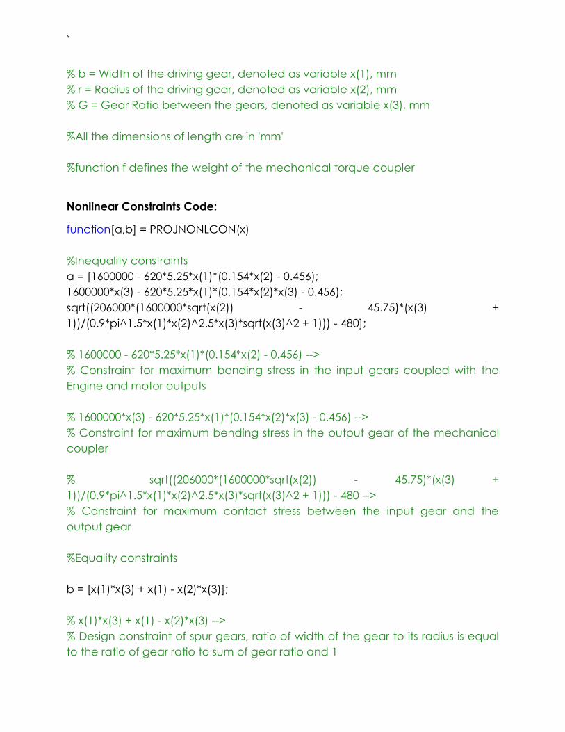
% b = Width of the driving gear, denoted as variable x(1), mm
% r = Radius of the driving gear, denoted as variable x(2), mm
% G = Gear Ratio between the gears, denoted as variable x(3), mm
%All the dimensions of length are in 'mm'
%function f defines the weight of the mechanical torque coupler
Nonlinear Constraints Code:
function[a,b] = PROJNONLCON(x)
%Inequality constraints
a = [1600000 - 620*5.25*x(1)*(0.154*x(2) - 0.456);
1600000*x(3) - 620*5.25*x(1)*(0.154*x(2)*x(3) - 0.456);
sqrt((206000*(1600000*sqrt(x(2)) - 45.75)*(x(3) +
1))/(0.9*pi^1.5*x(1)*x(2)^2.5*x(3)*sqrt(x(3)^2 + 1))) - 480];
% 1600000 - 620*5.25*x(1)*(0.154*x(2) - 0.456) -->
% Constraint for maximum bending stress in the input gears coupled with the
Engine and motor outputs
% 1600000*x(3) - 620*5.25*x(1)*(0.154*x(2)*x(3) - 0.456) -->
% Constraint for maximum bending stress in the output gear of the mechanical
coupler
% sqrt((206000*(1600000*sqrt(x(2)) - 45.75)*(x(3) +
1))/(0.9*pi^1.5*x(1)*x(2)^2.5*x(3)*sqrt(x(3)^2 + 1))) - 480 -->
% Constraint for maximum contact stress between the input gear and the
output gear
%Equality constraints
b = [x(1)*x(3) + x(1) - x(2)*x(3)];
% x(1)*x(3) + x(1) - x(2)*x(3) -->
% Design constraint of spur gears, ratio of width of the gear to its radius is equal
to the ratio of gear ratio to sum of gear ratio and 1

`
end
FMINCON SOLVER CODE:
function PROJOPT
clear all
clc
A=[ ];
b=[ ];
Aeq = [ ];
beq = [ ]; % matrix/vectors for defining linear constraints (not used)
lb = []; % lower bounds on the problem
ub = []; % upper bounds on the problem (not used)
xopt = fmincon('PROJFUN',[50,50,3],A,b,Aeq,beq,lb,ub,'PROJNONLCON');
[xopt,fval,exitflag,output,lambda,grad,hessian] =
fmincon('PROJFUN',[50,50,3],A,b,Aeq,beq,lb,ub,'PROJNONLCON');
fprintf('xopt = \n');disp(xopt)
fprintf('fval = \n');disp(fval)
fprintf('exitflag = \n');disp(exitflag)
fprintf('output = \n');disp(output)
fprintf('lambda = \n');disp(lambda)
fprintf('grad = \n');disp(grad)
fprintf('hessian = \n');disp(hessian)
% fprintf('lambda =');disp(lambda)
% fprintf('gradient =');disp(grad)
% fprintf('Hessian =');disp(hessian)
end
RESULTS AND PLOTS
1. Starting Point: [25 25 1]
i. Algorithm: Interior Point
Solution: b = 45.439; r = 74.509; G = 1.56; W = 27.4648

`
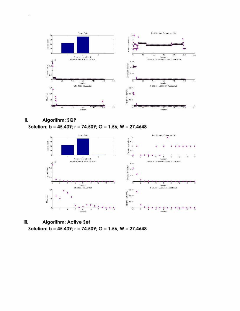
ii. Algorithm: SQP
Solution: b = 45.439; r = 74.509; G = 1.563; W = 27.4648
iii. Algorithm: Active Set
Solution: b = 45.439; r = 74.509; G = 1.56; W = 27.4648

`
2. Starting Point: [25 25 1]
i. Algorithm: Interior Point
Solution: b = 45.439; r = 74.509; G = 1.56; W = 27.4648
ii. Algorithm: SQP

`
Solution: b = 45.439; r = 74.509; G = 1.56; W = 27.4648
iii. Algorithm: Active Set
Solution: b = 45.439; r = 74.509; G = 1.56; W = 27.4648
3. Starting Point: [225 225 8]
i. Algorithm: Interior Point
Solution: b = 45.439; r = 74.509; G = 1.56; W = 27.4648
`
ii. Algorithm: SQP
Solution: b = 45.439; r = 74.509; G = 1.56; W = 27.4648
iii. Algorithm: Active Set
Solution: b = 45.439; r = 74.509; G = 1.56; W = 27.4648

`
CAD MODEL AND 2D DRAWINGS
3D CAD Model of the Optimized Input Gear

`
2D Drawings of the Input Gear
3D Model of the optimized Output Gear
`
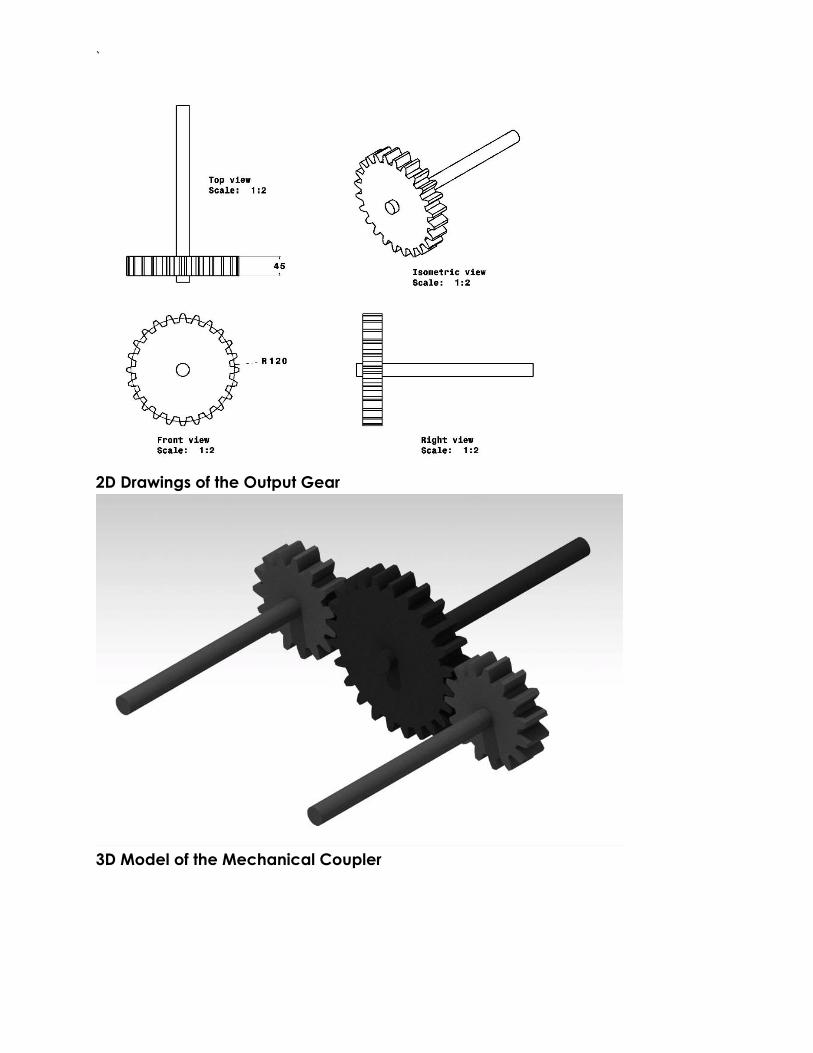
2D Drawings of the Output Gear
3D Model of the Mechanical Coupler
`
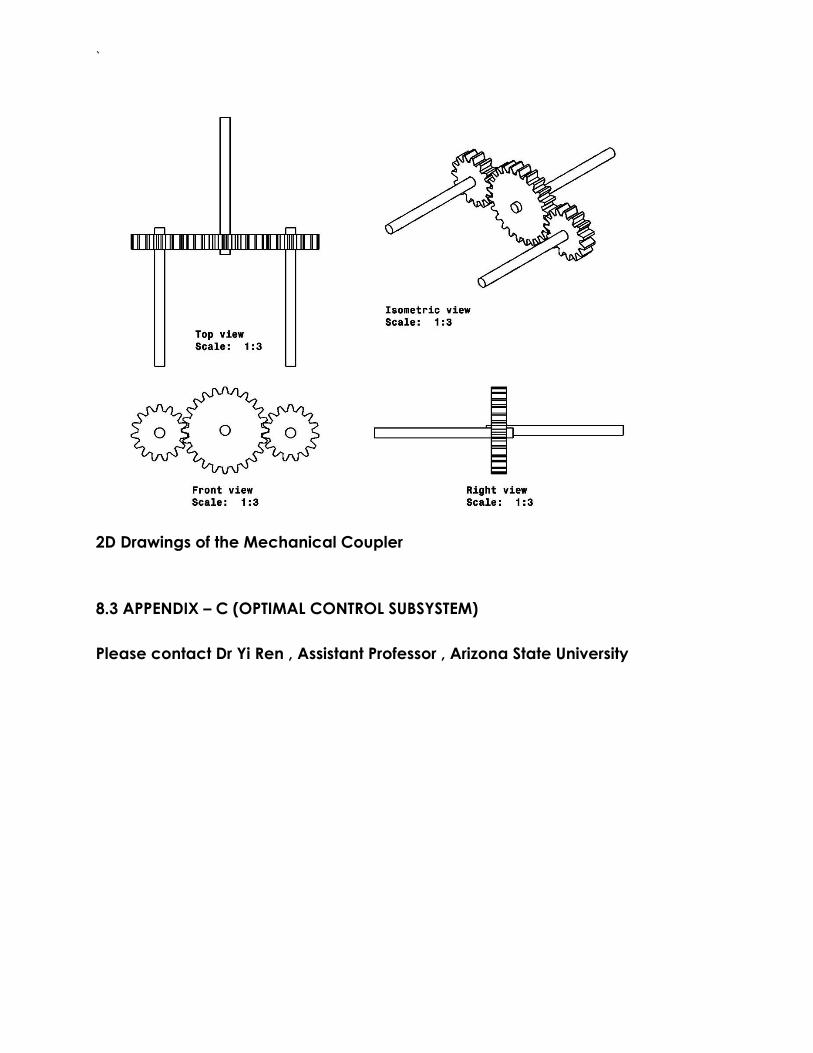
2D Drawings of the Mechanical Coupler
8.3 APPENDIX – C (OPTIMAL CONTROL SUBSYSTEM)
Please contact Dr Yi Ren , Assistant Professor , Arizona State University

`