UNLV Theses, Dissertations, Professional Papers, and Capstones

2009

Optimization of channel geometry in a protonexchange membrane (PEM) fuel cellJephanya KasukurthiUniversity of Nevada Las Vegas

Follow this and additional works at: http://digitalscholarship.unlv.edu/thesesdissertations

Part of the Energy Systems Commons, and the Oil, Gas, and Energy Commons

This Thesis is brought to you for free and open access by Digital Scholarship@UNLV. It has been accepted for inclusion in UNLV Theses, Dissertations,Professional Papers, and Capstones by an authorized administrator of Digital Scholarship@UNLV. For more information, please contactdigitalscholarship@unlv.edu.

Repository CitationKasukurthi, Jephanya, "Optimization of channel geometry in a proton exchange membrane (PEM) fuel cell" (2009). UNLV Theses,Dissertations, Professional Papers, and Capstones. 94.http://digitalscholarship.unlv.edu/thesesdissertations/94

OPTIMIZATION OF CHANNEL GEOMETRY IN A PROTON EXCHANGE

MEMBRANE (PEM) FUEL CELL

by

Jephanya Kasukurthi

Bachelor of Technology in Mechanical Engineering Acharya Nagarjuna University, India

2007

A thesis submitted in partial fulfillment

of the requirements for the

Master of Science Degree in Mechanical Engineering Department of Mechanical Engineering

Howard R. Hughes College of Engineering

Graduate College University of Nevada, Las Vegas

December 2009

ii

THE GRADUATE COLLEGE We recommend that the thesis prepared under our supervision by Jephanya Keerthi Swaroop Kasukurthi entitled Optimization of Channel Geometry in a Proton Exchange Membrane (PEM) Fuel Cell be accepted in partial fulfillment of the requirements for the degree of Master of Science Mechanical Engineering Yitung Chen, Committee Chair Robert Boehm, Committee Member Jianhu Nie, Committee Member Yahia Bagzhouz, Graduate Faculty Representative Ronald Smith, Ph. D., Vice President for Research and Graduate Studies and Dean of the Graduate College December 2009

iii

ABSTRACT

Optimization of Channel Geometry in a Proton Exchange Membrane (PEM) Fuel Cell

by

Jephanya Kasukurthi

Dr. Yitung Chen, Examination Committee Chair Professor of Department of Mechanical Engineering

University of Nevada, Las Vegas

Bipolar plates are the important components of the PEM fuel cell. The flow

distribution inside the bipolar plate should be uniform. Non-uniform flow distribution

inside the bipolar leads to poor performance of the fuel cell and wastage of expensive

catalyst. A single channel PEM fuel cell is taken and electrochemical analysis is carried

out on it. The results are compared with the available published experimental data

obtained by other research group, and they are found to be in good agreement. A baseline

design of the bipolar plate is taken and numerical analysis is carried out. The results show

that the flow distribution is non-uniform. The baseline design is changed to an improved

design to obtain a uniform flow. The improved design yielded a uniform flow. A single

channel is taken from the improved design of the bipolar plate and electrochemical

analysis is carried out on it. The geometry of the fuel cell channel is changed from

rectangular to square, semi-circle and triangular shapes and the performances of the fuel

cell are observed. The performance of the rectangular channel is found out to be the best,

and the performance of the triangular channel is poor compared to rectangular channel

design. The operating temperature of the fuel cell is varied and the results show that

increasing the fuel cell temperature from 323K to 353K increases the fuel cell

performance by 7.83%. Increasing the reaction temperature increases the thermal energy

iv

available in the system and all the molecules in the system move about and vibrate with

increased intensity increasing the rate of the reaction. The operating pressure of the fuel

cell is varied, and the performance of the fuel cell is observed. The performance of the

fuel increases by 2.35% when the pressure is increased by 2 atm on the anode side and 4

atm on the cathode side. The performance of the fuel cell increases due to a better supply

of reactants at higher pressures to active sites.

v

TABLE OF CONTENTS

ABSTRACT…… ............................................................................................................... iii LIST OF FIGURES .......................................................................................................... vii

LIST OF TABLES ............................................................................................................. ix

NOMENCLATURE ........................................................................................................... x

ACKNOWLEDGEMENTS ............................................................................................. xiii CHAPTER 1 INTRODUCTION ................................................................................... 1

1.1 Background ........................................................................................................ 1 1.2 Advantages and Disadvantages of a Fuel Cell .................................................... 2 1.3 Types of Fuel Cells ............................................................................................. 3 1.4 Basic Fuel Cell Operation ................................................................................... 6 1.5 PEMFC ............................................................................................................... 8 1.6 Performance of a Fuel Cell ................................................................................. 8 1.7 Literature Review.............................................................................................. 12 1.8 Research Objectives .......................................................................................... 19 1.9 Thesis Outline ................................................................................................... 19

CHAPTER 2 PEM FUEL CELL NUMERICAL MODEL VALIDATION ............... 20

2.1 Numerical model of PEM fuel cell .................................................................. 20 2.1.1 PEMFC Electrochemical Reactions ......................................................... 22 2.1.2 Charge Balances....................................................................................... 22 2.1.3 Mass Conservation Equations .................................................................. 25 2.1.4 Momentum Conservation Equations........................................................ 26 2.1.5 Species Conservation Equation................................................................ 26 2.1.6 Energy Conservation ................................................................................ 27

2.2 Numerical Model .............................................................................................. 28 2.2.1 Computational Domain ............................................................................ 28 2.2.2 Boundary Conditions ............................................................................... 31 2.2.3 PEMFC Model ......................................................................................... 32 2.2.4 Grid Independent Study ........................................................................... 36 2.2.5 PEMFC Model Validation ....................................................................... 36

CHAPTER 3 DESIGN OF UNIFORM FLOW BIPOLAR PLATE ........................... 40

3.1 Design Description............................................................................................ 40 3.2 Hydrodynamic Analysis.................................................................................... 44 3.3 Electrochemical Analysis.................................................................................. 49

CHAPTER 4 OPTIMIZATION OF PEMFC CHANNEL GEOMETRY ................... 54

4.1 Design Description............................................................................................ 54 4.2 Numerical Analysis ........................................................................................... 56

vi

4.3 Pressure Drop Calculation ................................................................................ 59 4.4 Temperature Variation ...................................................................................... 63 4.5 Pressure Variation ............................................................................................ 70

CHAPTER 5 CONCLUSIONS AND RECOMMENDATIONS ................................ 77

5.1 Conclusions ....................................................................................................... 77 5.2 Recommendations ............................................................................................. 78

REFERENCES… ............................................................................................................. 80 VITA………….. ............................................................................................................... 85

vii

LIST OF FIGURES

Fig. 1.1 Polarization curve of a fuel cell ........................................................................ 9 Fig. 2.1 Schematic view of PEMFC model ................................................................. 21 Fig. 2.2 Dimensions of single channel PEMFC ........................................................... 30 Fig. 2.3 Computational mesh ....................................................................................... 31 Fig. 2.4 Grid independent study ................................................................................... 36 Fig. 2.5 Comparison of the j-V curve of numerical model with experimental data .... 37 Fig. 2.6 Hydrogen mass fraction at the anode side ...................................................... 38 Fig. 2.7 Oxygen mass fraction at the cathode side ...................................................... 38 Fig. 2.8 Water mass fraction at the cathode side ......................................................... 39 Fig. 3.1 PEMFC baseline design.................................................................................. 41 Fig. 3.2 Dimensions of the baseline design of PEMFC ............................................... 41 Fig. 3.3(a) Computational mesh of the PEMFC .............................................................. 42 Fig. 3.3(b) Computational mesh of the channels and MEA ............................................ 43 Fig. 3.3(c) Mesh of bipolar plate and flow channels ....................................................... 43 Fig. 3.4 Flow distribution in the bipolar plate ............................................................. 44 Fig. 3.5 Improved design of PEMFC ........................................................................... 45 Fig. 3.6 Dimensions of improved design PEMFC ....................................................... 46 Fig. 3.7(a) Computational mesh of improved design PEMFC ....................................... 47 Fig. 3.7(b) Computational mesh of flow channels and the MEA .................................... 47 Fig. 3.7(c) Mesh of bipolar plate and channels ................................................................ 48 Fig. 3.8 Flow distribution inside the channels of the improved design of PEMFC ..... 49 Fig. 3.9 Computational domain ................................................................................... 50 Fig. 3.10 Temperature distribution along the cathode gas channel ............................... 50 Fig. 3.11 Temperature distribution along the anode gas channel .................................. 51 Fig. 3.12 Hydrogen mass fraction at the anode channel ............................................... 52 Fig. 3.13 Oxygen mass fraction at the cathode gas channel .......................................... 52 Fig. 3.14 Water mass fraction at the cathode gas channel ............................................. 53 Fig. 4.1 Rectangular channel ....................................................................................... 54 Fig. 4.2 Square channel ................................................................................................ 54 Fig. 4.3 Semi-circular channel ..................................................................................... 55 Fig. 4.4 Triangular channel .......................................................................................... 56 Fig. 4.5 j-V curves of different channel geometries .................................................... 57 Fig. 4.6 Power density curves of different channel geometries ................................... 59 Fig. 4.7 Aspect ratio calculation for different geometries ........................................... 61 Fig. 4.8 Velocity vector plot in the channel ................................................................. 62 Fig. 4.9 j-V curves of the rectangular channel at different temperatures ................... 64 Fig. 4.10 Power density curves of the rectangular channel at different temperatures . 65 Fig. 4.11 j-V curves of the square channel at different temperatures .......................... 66 Fig. 4.12 Power density curves of the square channel at different temperatures ......... 67 Fig. 4.13 j-V curves of the semi-circle channel at different temperatures ................... 65 Fig. 4.14 Power density curves of the semi-circle channel at different temperatures . 66 Fig. 4.15 j-V curves of the triangular channel at different temperatures ...................... 66 Fig. 4.16 Power density curves of triangular channel at different temperatures .......... 68 Fig. 4.17 j-V curves of the rectangular channel at various operating pressures ........... 70

viii

Fig. 4.18 Power density curves of rectangular channel at various operating pressures 71 Fig. 4.19 j-V curves of the square channel at various operating pressures .................... 71 Fig. 4.20 Power density curves of the square channel at various operating pressures .. 72 Fig. 4.21 j-V curves of the semi-circular channel at various operating pressures ......... 72 Fig. 4.22 Power density curves of semi-circular channel at various operating pressures........................................................................................................................................... 73 Fig. 4.23 j-V curves of the triangular channel at various operating pressures ............... 73 Fig. 4.24 Power density curves of triangular channel at various operating pressures .... 74

ix

LIST OF TABLES

Table. 2.1 Dimensions of single channel PEMFC model ............................................ 29 Table. 2.2 PEMFC parameters ..................................................................................... 33 Table. 4.1 Pressure drop comparison ........................................................................... 63 Table. 4.2 Slopes of the j-V curves at different temperatures ..................................... 68 Table. 4.3 Slopes of the j-V curves at different operating pressures ........................... 75

x

NOMENCLATURE

a water activity

mA , chA membrane area and channel cross section area (m2)

b Tafel slope

c molar concentration (g-mole/cm3)

ijD binary diffusivity (cm2/s)

0E standard potential under 25 oC, 1 atm

F Faraday constant (96487 C/mol)

0G∆ standard free energy (kJ/mol)

H∆ stored chemical energy (kJ/mol)

I , refI current (A) and reference current (A/m2)

j current density (A/m2)

solj , memj solid phase and membrane phase current density (A/m2)

refanj , ref

catj volumetric reference exchange current density (A/m2)

K absolute permeability (cm2)

rK relative permeability

effk effective heat conductivity (W/m-K)

2,HwM molecular weight of hydrogen (g/mol)

OHwM2, molecular weight of water (g/mol)

2,OwM molecule weight of oxygen (g/mol)

N molar flux vector (g-mol/cm2-s)

n unit vector

xi

cp capillary pressure (Pa)

2Hp ,2Op hydrogen and oxygen gas pressure (Pa)

R gas constant (8.314 J/K-mol)

tolR fuel cell total electric resistance (ohm)

wr condensation rate (kg/s)

s liquid water saturation

T absolute temperature (K)

iU velocity vector (m/s)

cellV fuel cell operating voltage (V)

ocV fuel cell open circuit voltage or ideal voltage (V)

w weight fraction

X , ix molar fraction and molar fraction of species i

aα , cα anode and cathode transfer coefficient

ε porosity

solσ , memσ solid and membrane field conductivity (Siemens)

σ surface tension (N/m2)

solφ , memφ solid phase and membrane field potential (V)

ϕ , iϕ fuel cell efficiency and ideal fuel cell efficiency

γ concentration dependence

masη mass transport limit loss potential (V)

ohmη ohmic loss potential (V)

xii

polη activation loss potential (V)

iρ density of component i (kg/m3)

aς , cς anode and cathode stoichiometric ratio

iµ viscosity of component i (kg/m-s)

lµ liquid water viscosity (kg/m-s)

xiii

ACKNOWLEDGEMENTS

I would like to express profound gratitude to my advisor, Dr. Yitung Chen, for his

invaluable support, encouragement, supervision and useful suggestions throughout this

research work. His moral support and continuous guidance enabled me to complete my

work successfully. This thesis would not have been possible without the kind support, the

trenchant critiques, the probing questions, and the remarkable patience of my thesis

advisor. I cannot thank him enough. I am also highly thankful to Dr. Jianhu Nie for his

valuable suggestions throughout this study.

I would like to thank Dr. Robert F Boehm and Dr. Yahia Baghzouz for their time to

review the thesis and for participation as defense committee members.

I am as ever, especially indebted to my parents, Dr. Ratna Raju and Mrs. Ruth

Vindhya Vasini Kasukurthi for their love and support throughout my life. I am also

thankful to my friends who made my life happy away from home

1

CHAPTER 1

INTRODUCTION

1.1 Background

Due to increasing pollution and depletion of the natural fuel resources an

alternative for the energy sources have to be found out, in this process of uncovering the

alternative fuel source, hydrogen energy has been found out [1]. The device which uses

hydrogen as the fuel called fuel cell has been discovered in this process. It is believed that

hydrogen can be a future solution to world’s energy needs. “Fuel cell” is a device that

combines hydrogen and oxygen to form water and electricity [1]. The produced energy

can be used for our day to day needs. Fuel cells have many advantages when compared

with the conventional devices. A Fuel cell has very high efficiency, and it is not limited

by Carnot cycle efficiency [2]. Fuel cells are quiet and pollution free.

The development of the fuel cell began long back. In 1838 C.F.Schonbein

developed “Fuel Cell theory” [3]. He conducted experiments and published results of

producing electrical current using hydrogen and chlorine or oxygen gas on the platinum

electrode and called this effect as “Polarization effect”. In 1839 William R. Grove

discovered “gas voltaic battery” [3]. He found that electrical energy is needed for

producing hydrogen and oxygen gases from water electrolysis process and proposed that

electrical energy can be produced from the reverse process. In 1889 L.Mond and C.

Langer proposed the terminology of fuel cell. In 1902 Reid proposed the “alkaline fuel

cell” concept [3]. In 1923 A. Schmidt proposed the “porous gas diffusion electrode”

concept. Many developments took place after that. In 1966 DuPont developed the

“Nafion” polymer or proton exchange membrane (PEM) [4]. In 1970 U.S. Department of

2

Energy developed molten carbonate fuel cell. In 1981 Westinghouse developed a solid

oxide fuel cell. In 2003, 17 countries formed an international partnership for hydrogen

economy (IPHE) to promote hydrogen energy and fuel cell technology research [4].

1.2 Advantages and Disadvantages of a Fuel Cell

A fuel cell is a device which combines hydrogen and oxygen to form water by

electrochemical reaction and in this process electricity is produced. The battery is the

electrochemical device we are familiar with. The chemicals stored in a battery are

converted into electricity and go dead after they are used. The fuel cell works until the

fuel is supplied continuously. There are many advantages for fuel cell. Fuel cell combines

many advantages of both engines and batteries [2]. Fuel cells are more efficient than

combustion engines because they produce electricity directly from chemical energy. Fuel

cells don’t have any moving parts, so they are silent and mechanically ideal. The fuel

cells are clean because they don’t emit harmful emissions. Fuel cells operate with higher

energy densities compared to batteries and can be quickly recharged by refueling. There

are some disadvantages of using fuel cells. Fuel cells are very expensive. The power

density of fuel is less when compared with combustion engines and batteries. The fuel for

the fuel cell is hydrogen. Hydrogen is not abundantly available, and the storage of

hydrogen is also not easy. The operation temperatures are not compatible. Fuel cells are

susceptible to environment poisons.

3

1.3 Types of Fuel Cells

There are five major types of fuel cells, differentiated from one another by their

electrolyte:

1. Phosphoric acid fuel cell (PAFC)

2. Proton exchange membrane or polymer electrolyte membrane fuel cell (PEMFC)

3. Alkaline fuel cell (AFC)

4. Molten carbonate fuel cell (MCFC)

5. Solid oxide fuel cell (SOFC)

In 1961, G. V. Elmore and H. A. Tanner revealed new promise in phosphoric acid

electrolytes in their paper “Intermediate Temperature Fuel Cells”, the stepping stone for

phosphoric acid fuel cells [4]. Phosphoric acid fuel cells (PAFC) use phosphoric acid as

the electrolyte and platinum as the catalyst. These fuel cells operate at a temperature

range of around 160-2000C. The efficiency of these fuel cells is around 37-42% [4]. The

advantage of these fuel cells is that they can tolerate a carbon monoxide concentration of

about 1.5%. Another advantage is that concentrated phosphoric acid electrolyte can

operate above the boiling point of water, a limitation on other acid electrolytes that

require water for conductivity. The application of these fuel cells is that they can be used

for a thermal–electrical cogeneration power plant.

Proton exchange membrane fuel cell (PEMFC) is also called the polymer

electrolyte membrane fuel cell. These fuel cells use proton conducting polymer

membrane as electrolyte. Proton exchange membrane fuel cells operate at very low

temperatures around 800C. PEMFC uses hydrogen as fuel and air as the oxidant and

produces water as the by-product. These fuel cells are very useful because they operate at

4

low temperatures and high power density. The efficiency of these fuel cells is around 43

– 58 % [4]. PEMFC uses platinum as the catalyst. These fuel cells can mainly be used for

transportation and automotive applications, so these fuel cells play a vital role for

reducing the pollution of atmosphere. Proton exchange membrane fuel cells operate at

very moderate temperatures, so they have low carbon monoxide tolerance which is a

problem of poisoning of the catalyst (i.e. platinum) of the fuel cell.

Alkaline fuel cells (AFC) were developed in mid 1960’s by NASA for the Apollo

and space shuttle programs [4]. Alkaline fuel cells use an electrolyte that is an aqueous

(water-based) solution of potassium hydroxide (KOH) retained in a porous stabilized

matrix. The concentration of KOH can be varied with the fuel cell operating temperature,

which ranges from 65°C to 220°C [4]. The charge carrier for an AFC is the hydroxyl ion

(OH-) that migrates from the cathode to the anode where it reacts with hydrogen to

produce water and electrons. These are the cheapest fuel cells to manufacture when

compared with other types of fuel cells. The disadvantage of these fuel cells is that they

are very sensitive to carbon dioxide that may be present in fuel or air. The carbon dioxide

reacts with the electrolyte, poisons it rapidly, and severely decreases the performance of

the fuel cell. Due to these reasons the alkaline fuel cells are confined to closed

environments such as space and undersea vehicles. Pure hydrogen and oxygen should be

used for running these fuel cells. Alkaline fuel cells are not considered for automobile

applications because of their sensitivity to poisoning.

Molten carbonate fuel cells (MCFC) are in the class of high temperature fuel

cells. These fuel cells operate around a temperature of around 6500C [4]. These fuel cells

use an electrolyte composed of a molten mixture of carbonate salts. When these salts are

5

heated around 6500C they melt and become conductive to carbonate ions (CO32-). These

ions flow from cathode to the anode where they combine with hydrogen to give water,

carbon dioxide and electrons. The advantage of this fuel cell is that internal reforming is

possible due to its high operating temperature. These fuel cells need significant time to

reach the high temperature and respond slowly to power demands so these are suitable for

constant power applications.

The solid oxide fuel cell (SOFC) is currently the highest temperature fuel cell in

development. SOFC operates in a temperature range of 6000C – 10000C [4]. Different

kinds of fuels can be used because of the operating temperature. To operate at such high

temperature these fuel cells use solid ceramic material (solid oxide) as the electrolyte

material which is conductive to oxygen ions (O2-). The charge carrier in the SOFC is the

oxygen ion (O2-). The operating efficiency of this fuel cell is highest, about 60% [4]. The

high temperature of these fuel cells enables them to tolerate impure fuels such as those

obtained from the gasification of coal or gasses from industrial processes. The startup

time for these fuel cells is the main drawback, these fuel cells require significant amount

of time to reach the operating temperature and respond slowly to the changes in

electricity demand. Therefore these fuel cells are considered to be a leading candidate for

high-power applications such as industrial and large-scale central-electricity generating-

stations. These fuel cells require expensive materials for construction due to their high

operating temperatures.

6

1.4 Basic Fuel Cell Operation

The electricity produced by a fuel cell increases with increase in reaction area. To

provide large reaction surfaces fuel cells are usually made as thin and planar structures.

One side of the planar structure of fuel cell is supplied with fuel and other side of the fuel

cell is supplied with oxidant. A thin layer called electrolyte separates the fuel and

electrodes and ensures that the two individual half reactions occur in isolation from one

another. The major steps involved in producing electricity in a fuel cell are [2]:

1. Reactant delivery

2. Electrochemical reaction

3. Ionic conduction through the electrolyte and electronic conduction through the

external circuit

4. Product removal from the fuel cell

Reactant transport: A fuel cell produces electricity when it is continuously supplied with

fuel and oxidant. This seems to be a simple task but it is a very complicated process.

When the fuel cell is operated at high current the demand for the reactants is very high.

The reactants should be supplied rapidly otherwise the fuel cell will starve. The delivery

of reactants can be effectively done by using the flow channels. The flow structures

significantly affect the performance of the fuel cell [2]. The flow structure plays a vital

role in the fuel cell performance because mass transport of the reactants can be controlled

by the flow structure.

Electrochemical reaction: Immediately after the delivery the reactants should undergo

electrochemical reaction. The current generated by the fuel cell depends on how fast the

electrochemical reactions take place [2]. The faster the electrochemical reactions the

7

more is the current produced. The current produced is more if the electrochemical

reaction is fast. High current from the fuel cell is desirable so catalysts are used to

increase the speed and efficiency of the electrochemical reactions. The fuel cell

performance vitally depends on choosing the right catalyst and carefully designing the

reaction zones.

Ionic and electronic conduction: The electrochemical reactions produce or consume ions

and electrons. Ions produced at one electrode must be consumed at the other electrode.

This is also same for electrons. To maintain charge balance the electrons and ions must

be transported from the place they are produced to the place they are consumed.

Electrons can be transported easily whereas the transportation of ions is a tough task

because ions are much larger and massive than electrons.

Product Removal: The fuel cells produce electricity with some by products for example

H2-O2 fuel cell generate water, hydrocarbon fuel cells generate carbon dioxide (CO2).

The byproducts formed from the electrochemical reactions should be removed from time

to time otherwise they will build up and eventually strangle the fuel cell and prevents

new fuel and oxidant from reacting. The product removal is not one of the major issues of

fuel cell designing but in PEMFC when the water is not removed it causes flooding of the

fuel cell.

8

1.5 PEMFC

PEM stands for polymer electrolyte membrane or proton exchange membrane. A

polymer membrane is present in the fuel cell so it is called a polymer electrolyte

membrane. The polymer membrane has unique capabilities. It is impermeable to gases

but it conducts protons so it is called a proton exchange membrane. The membrane is

coated with thin layers of catalyst on either side and sandwiched between two porous gas

diffusion layers (GDL) and these are collectively called as membrane electrode assembly

which is place between two bipolar plates which supply fuel and oxidant for

electrochemical reaction. The electrodes are manufactured with carbon cloth or carbon

fiber paper. The catalyst material is platinum supported on carbon [4]. Electrochemical

reaction takes place at the surface of the catalyst at the interface between the electrolyte

and the membrane. Hydrogen is fed to the fuel and it splits into protons and electrons.

The protons travel through the membrane where as the electrons travel through the

collectors and external circuit to produce electricity. The protons formed from the

hydrogen combine with the oxygen ions and produce water. The hydrogen side is

negative and it is called the anode, whereas the oxygen side of the fuel cell is positive and

it is called cathode.

1.6 Performance of a Fuel Cell

The performance of a fuel cell can be clearly identified from the graph of its

current-voltage characteristics. The graph is called current density-voltage (j-V) curve,

and it shows the voltage output of the fuel cell for a given current input. This curve is

also called the polarization curve which is shown in Fig 1.1. The x-axis shows current

9

density i.e. current has been normalized by fuel cell area. Current density is used because

a larger fuel cell can produce more electricity than a smaller fuel cell so that j-V curves

are normalized by fuel cell area to make results comparable.

Fig 1.1 Polarization curve of a fuel cell

An ideal fuel cell continues to supply current until it is supplied with sufficient

amount of fuel maintaining the constant thermodynamic voltage. The actual output of a

real fuel cell is less than the ideal voltage or thermodynamic voltage. The voltage output

of the fuel cell influences the total power produced. The power produced by the fuel cell

is the product of current and voltage, P = iV. The power density curve gives the power

density delivered by a fuel cell as a function of current density. The current supplied by a

fuel cell is directly proportional to the amount of fuel consumed (i.e., if the fuel cell

voltage decreases, the electric power produced by the fuel cell also decreases). By this

relation we can say that fuel cell voltage is a measure of fuel cell efficiency. It is very

important to maintain a constant voltage to have higher efficiency. It is very hard to

maintain constant voltage due to the irreversible losses. The more the current drawn from

10

the fuel cell, the more are the losses. There are three major types of fuel cell losses which

give the polarization curve the characteristic shape which can be seen in Fig.1.1. The

three major losses are [2]:

a) Activation loss

b) Ohmic loss

c) Concentration loss

a) Activation loss:

The voltage which is sacrificed to overcome the activation barrier is called as the

activation loss and it is represented as ηact. The Butler-Volmer equation is used to

describe how current and voltage are related in electrochemical systems. The Butler-

Volmer equation states that the current produced by an electrochemical reaction increases

exponentially with activation overvoltage. This explains that if we want more current

from the fuel cell we must pay a price in terms of lost voltage.

� � ����

���

���� �� ����⁄ �

���

���� ������� ����⁄ � (1-1)

where � is the voltage loss, � is the number of electrons transferred in the

electrochemical reaction, ��� and ��

� are the actual surface concentrations of the rate-

limiting species in the reaction, ���� and ��

�� are the product concentration values, ���

represents the exchange current density at a standard concentration, F is Faraday constant

and R and T are the gas constant and cell absolute temperature, α is the transfer

coefficient. The empirical relationship between the activation overvoltage and the current

density is given by the Tafel equation

���� � � � � log � (1-2)

11

where � is the constant, � is the Tafel slope, and j is the current density.

b) Ohmic loss:

The voltage expended in order to accomplish charge transport is called the ohmic

loss. It is represented as �#$%&�.

From Ohm’s law

�#$%&� � ()#$%&� � (�)*+*� � )&#�&�� (1-3)

where i is the current, and )*+*� and )&#�&� are the electronic and ionic resistances

offered by the fuel cell. The electronic and ionic resistances depend on the material of

the membrane.

c) Concentration loss:

The concentration loss is minimized by the careful optimization of mass transport

in the fuel cell electrodes and fuel cell flow structures. It is represented as ��#��.

��#�� � � ln-.

-.�- (1-4)

where c is a constant which can be approximately given as

� ���

���1 �

�

� (1-5)

�0 is the limiting current density which can be given as below

�0 � �12*33 ��4

5 (1-6)

2&-*33

� 6�.72&- (1-7)

12

where F is Faraday constant, 2&- is the binary diffusion coefficient (cm2/s), ε is the

porosity of the porous structure, Deff is the effective diffusivity, ��# is the concentration of

the reactants, n is the number of electrons transferred and 8 is the gas diffusion layer

thickness.

Fig.1.1 shows the polarization curve which has three regions activation, ohmic

and mass transport region which are influenced by the losses in the fuel cell. The

activation loss is predominant in the activation region of the polarization curve. The

electrode kinetics controls the activation region. The loss at the ohmic region of the

polarization curve is due to the ionic and electronic resistances provided by the fuel cell.

The concentration loss is most significant at the tail of the polarization curve (i.e., in the

mass transport region). This loss is due to the mass transport configuration of the fuel

cell.

1.7 Literature Review

The physics involved in a fuel cell are very complicated. There are many

processes simultaneously occurring in a PEM fuel cell. It is difficult to study every

process that is involved in a fuel cell. Different researchers have concentrated on different

aspects of fuel cell. The experimental setup for a fuel cell is very expensive so

computational fluid dynamics (CFD) modeling has played a major role in the fuel cell

research. The CFD model should be coupled with an electrochemical model to predict the

species transport and electrochemical reactions.

Large numbers of numerical models of fuel cells have been developed by many

researchers from the dawn of CFD. First the researchers have concentrated only on the

13

specific parts of the PEM fuel cell such as the bipolar plate, catalyst layer, gas diffusion

layer and membrane. Some years back there was limited computational power so only a

one- dimensional numerical model of PEM fuel was developed by Bernardi et al. [5] and

the results were compared with experimental results. Later, two-dimensional numerical

models were developed. The two-dimensional and one-dimensional models are only used

to estimate the fuel cell performance but not very accurate. After the increase in

computational power the three-dimensional models have been developed to analyze the

fuel cell operation.

The three-dimensional models can approximately predict the behavior of the PEM

fuel cell, but the processes involved in the fuel cell are very complicated so some

assumptions have to be considered to simplify the modeling of the fuel cell. Dutta et al.

[6] and Berning et al. [7] developed the three-dimensional models and have done research

on them. Berning et al. [7] have performed parametric study for 3-D model of the PEM

fuel cell and compared with experimental results obtained by Ticianelli et al. [8]. The

experimental results obtained by Ticianelli et al. [8] have been used by many researchers

to validate their numerical results. Djilali et al. [9], [10] discussed about the advanced

computational tools for designing PEM fuel cell in two papers. Mann et al. [11]

developed an electrochemical model of the PEM fuel cell and compared the results with a

commercial Ballard PEM fuel cell. Nguyen et al. [12] developed a three-dimensional

CFD model of a PEM fuel cell with serpentine flow field. They implemented a voltage-

to-current (VTC) algorithm that solves for the potential as well as the local activation

potential.

14

The PEM fuel cell consists of many parts such as bipolar plates, gas diffusion

layers, catalyst layers and membrane. Every part plays an important role in the operation

of the fuel cell. It is difficult to concentrate on every part so many researchers have

concentrated on one of the parts or an aspect of the fuel cell. The bipolar plate has many

functions such as supplying the fuel, draining out the byproduct water and collecting the

current produced. The design of the flow structure that is present in the bipolar plate

plays an important role in the performance of the fuel cell. There are many types of flow

field designs: (1) parallel channel, (2) serpentine channel, (3) parallel serpentine channel,

and (4) interdigitated channel. The fuel should be distributed uniformly otherwise there

will be poor performance and inefficient use of the very expensive catalyst.

The serpentine flow field is mostly commonly used for a PEM fuel cell. Dutta et

al. [13] developed a model to predict the mass flow between channels in a polymer

electrolyte membrane (PEM) fuel cell with a serpentine flow path. Kazim et al. [14]

developed a simple mathematical model to investigate the superiority of the interdigitated

flow field design over the parallel flow field. The results obtained from their study show

that the interdigitated flow field can double the maximum power density of a PEM fuel

cell when compared with the parallel flow field. The modeling results agreed well with

the experimental studies in their study. Park et al. [15] conducted numerical and

experimental study to investigate the cross flow in a PEM fuel cell.

Grigoriev et al. [16] dealt with numerical optimization of the dimensions of

channels and current transfer ribs of bipolar plates. The material of the bipolar plate also

plays an important role in the performance of the fuel cell. Wind et al. [17] have done the

research on using stainless steel as the material for the bipolar plate. Stainless steel with

15

thin coatings is suggested for the PEM fuel cell because the performance of the fuel cell

with graphite bipolar plates is same as that of the fuel cell with coated metallic bipolar

plates. Two types of carbon composite materials are developed by Cho et al. [18].

The membrane is the main component in PEM fuel cell. The fuel cell is named

from the membrane’s properties as proton exchange membrane or polymer electrolyte

membrane. The membrane must exhibit properties such as high proton conductivity and

low ionic conductivity, it should also act as a barrier to mixing of fuel and reactant gases,

and it must be chemically and mechanically stable in the fuel cell environment. The

membranes for PEM fuel cells are made of perflurocarbon-sulfonic acid ionomer (PSA).

The best known membrane material is Nafion® made by Dupont. The protonic

conductivity of a polymer membrane is strongly dependent on its membrane structure and

its water content. The protons from one side of the membrane are dragged to the other

side of the membrane with the help of water (called electroosmotic drag). Sgrecciaa et al.

[19] developed self-assembled nano composite organic–inorganic proton conducting

sulfonated poly-ether-ether-ketone (SPEEK)-based membranes for PEM fuel cells.

Different strategies have been explored by them to improve water retention and

morphological stability of sulfonated aromatic polymers. Mechanical and thermal

properties, water uptake, and proton conductivity of the new membrane material are

reported.

Yan et al. [20] conducted water balance experiments on the membrane of the fuel

cell and found out that the net drag coefficient of water through the membrane depended

on current density and humidification of feed gases. The diffusion of water across Nafion

membranes was also investigated by experimental water flux measurements. PEM

16

membrane requirements are discussed in terms of two different parameters: temperature

and relative humidity by Beuscher et al. [21]. Additional advancements will be necessary

to meet aggressive operating conditions of higher temperatures and/or lower humidities,

as well as longer operating lifetimes. In this paper, these challenges for fuel cell

membranes are considered. The effect of operating parameters on the proton conductivity

of PEM fuel cell membranes and the resulting effect on fuel cell performance are

examined using experimental observations. Numerical simulations are used to assess the

influence of water transport properties on the local hydration state of the membrane

inside the running fuel cell.

The gas diffusion layer (GDL) is one of the critical components acting both as the

functional as well as the support structure for membrane–electrode assembly in the

proton exchange membrane fuel cell (PEMFC). Cindrella et al. [22] have studied the

importance of the GDL of the PEMFC, reviewed the essential properties of the GDLs,

and considered the methods of achieving each one of them. The paper also discusses the

key parameters of the GDL such as structure, porosity, hydrophobicity, hydrophilicity,

gas permeability, transport properties, water management and the surface morphology.

They conducted extensive research and found out that it is very important to develop

highly functionalized GDL with self–adjusting characteristics of water retention and

water draining along with structural features to steadily supply the reactant gases to the

catalyst.

Niu et al. [23] developed a multiphase, multiple-relaxation-time lattice Boltzmann

model to study water-gas transport processes in the gas diffusion layer of a PEM fuel cell.

The model is based on the diffuse interface theory, and employs two distributions so that

17

multiphase flows with large density ratios and various viscosities can be handled. In this

paper water-gas transportation in a three-dimensional modeled GDL structure is

simulated and the transport properties including absolute and relative permeabilities are

calculated. Benziger et al. [24] studied how the water flows in a GDL of a PEM fuel cell.

They conducted experiments and measured how the water flows through the GDL. They

also found out how much pressure is required for the water transport through the GDL.

They studied the pores that are present in the GDL and found the optimum pressure that

is required to drain the water through the largest pores.

One of the most important parts of the PEM fuel cell is the catalyst layer. The

electrochemical reactions take place on the surface of the catalyst. This is because three

kinds of species participate in the electrochemical reactions namely gases, electrons and

protons. Therefore the reactions take place on a portion of the catalyst where all the three

species have access. The material used for the catalyst layer of PEM fuel cells is

platinum. Zhang et al. [25] in their paper discuss the impact of degradation of the

catalyst. This paper reviews the recent research on degradation and durability issues in

the catalyst layers. They also suggested many experimental methods and investigation

techniques for evaluating catalyst degradation.

Zhang et al. [26] performed quantitative analysis of catalyst layer degradation

with X-ray photoelectron spectroscopy (XPS). XPS is quantitative, surface-sensitive, and

able to distinguish different bonding environments or chemical states of fuel cell catalyst

layers. The above capabilities are used to explore the complex mechanisms of

degradation during fuel cell operation. Das et al. [27] developed a three–dimensional

agglomerate model for cathode catalyst layer of PEM fuel cell. A finite element

18

technique is used for the numerical simulation is developed. Three configurations of

agglomerate arrangements are simulated to investigate the oxygen transport process

through the cathode catalyst layer and its impact on the activation polarization.

Hartnig et al. [28] worked on investigation of water drop kinetics and

optimization of channel geometry for PEM fuel cell cathodes. The paper discussed about

employing different flow field channel geometries and compared by means of a

simplified parametric identification. The rectangular shaped channel with a width of 1

mm and a depth of 0.5 mm is found to exhibit best water removal properties at a

reasonable pressure drop. Kuo et al. [29] performed numerical simulations to evaluate the

convective heat transfer performance and velocity flow characteristics of gas flow

channel design to enhance the performance of PEM fuel cell. The flow channel geometry

is not changed but induced different types of interruptions for the gas channel. They

implemented different types of obstacles such as wave like, trapezoid like and ladder like

forms and straight channel. The numerical results obtained show that the channels with

interruptions like wave, trapezoid and ladder like geometries increase the gas flow

velocity in the channel and improve the catalysis reaction performance in the catalyst

layer.

Wang et al. [30] developed a three-dimensional numerical model to explore the

effects of the cathode flow channel configuration. They have found that the interdigitated

design has superior cell performance over the parallel design for all the conditions

considered. Their study considered the effects of the flow channel aspect ratio and flow

channel cross-sectional area. They also found that the optimal flow channel aspect ratio is

1 and optimal cross-sectional area is 1mm x 1mm for the best cell performance.

19

1.8 Research Objectives

• Create a single channel PEMFC numerical model with the nine zones of two

bipolar plates, two gas channels, two gas diffusion layers, two catalyst layers and

a membrane.

• Simulate the hydrodynamic, heat transfer and electrochemical phenomena and

obtain the fuel cell performance and validate the model using available published

experimental data.

• Design bipolar plates with uniform flow distribution and take a single channel and

carry out analysis on the single channel.

• Change the channel geometry of the fuel cell and compare the performance.

1.9 Thesis Outline

In this thesis, the channel geometry in a PEMFC is optimized and the

performance studied. Chapter 2 explains the PEMFC modeling and the fundamentals of

the electrochemistry involved in a fuel cell. The developed model is validated using a

three-dimensional single channel PEMFC case. Chapter 3 discusses about designing a

uniform flow bipolar plate for a PEMFC. Chapter 4 focuses on optimizing the channel

geometry in a PEMFC. Chapter 5 concludes the current research and provides some

future recommendations.

20

CHAPTER 2

PEM FUEL CELL NUMERICAL MODEL VALIDATION

2.1 Numerical Model of PEM Fuel Cell

A schematic view of the system considered is shown in Fig.2.1. A PEM fuel cell

consists of nine zones. They are two gas channels, two bipolar plates, two gas diffusion

layers, two catalyst layers and a membrane. The membrane is placed between two

catalyst layers and then these are sandwiched between the gas diffusion layers and this

assembly is placed between two bipolar plates. The bipolar plates consist of flow

channels which provide fuel and oxidant for electrochemical reaction to take place. The

fuel and oxidant diffuse from their respective sides through the gas diffusion layers and

reactions take place at the catalyst layers and break down into ions and electrons. The

electrons are collected and passed through an external circuit to produce electricity. The

hydrogen ions formed from the electrochemical reaction combine with oxygen ions

formed from the electrochemical reaction on the other side to form water. The chemical

reactions that take place in the fuel cell are:

At anode: 2H2 (g) 4H++ 4e- (2-1)

At cathode: 4H++4e-+O2 (g) 2H2O (l) (2-2)

Overall: 2H2 (g) +O2 (g) 2H2O (l) (2-3)

21

Fig 2.1 Schematic view of a typical PEMFC

The physics involved in a fuel are very complicated. To replicate a model of a

fuel cell it is required to understand the mass, momentum and energy transport,

electrochemical reactions and charge balance inside the fuel cell. To simplify the

numerical modeling some assumptions are considered. They are:

� Ideal gas mixtures

� Steady state operation

� Isotropic electrodes and membrane

� Negligible contact resistance of current collector and MEA

� Incompressible flow

22

2.1.1 PEMFC Electrochemical Reactions

The electrochemical reactions involve both a transfer of electrical charge and a

change in Gibbs energy. The rate of an electrochemical reaction is determined by an

activation barrier. The speed at which an electrochemical reaction proceeds is the rate at

which the electrons are released, which is the electrical current. Current density is the

current per unit area of the surface. According to Faraday’s law current density is

proportional to the charge transferred and consumption of reactant per unit area [2].

( � �19 (2-4)

where �:; :< � 9� ⁄ is the rate of the electrochemical reaction (mol/s), F is the Faraday’s

constant, n is the number of moles of electrons transferred during the electrochemical

reaction.

2.1.2 Charge Balances

The electronic charge balance in the anode and cathode current collectors is given

by

( ) 01 =∇−•∇ elecφσ (2-5)

where 1σ denotes the electronic conductivity of the current feeder and elecφ is its

electronic potential.

The charge balance for the membrane is given by

( ) 02 =∇−•∇ ionicφσ (2-6)

where 2σ is the ionic conductivity and ionicφ is the potential in the membrane.

23

The electrochemical reactions take place on the surface of the catalyst and the

protons are transferred through the membrane and the electrons are transferred back to

the anode current collector. The electrons reach the cathode current collector through an

external circuit. The charge balance is given by [31].

( ) ictaelec iS=∇−•∇ φσ1 (2-7)

( ) ictaion iS=∇−•∇ φσ 2 (2-8)

where ictaiS denotes the specific surface area aS times the charge transfer current

reaction densityicti .

To solve the equations the boundary conditions are specified as:

0=elecφ (anode) (2-9)

cellelec V=φ (cathode) (2-10)

Butler-Volmer charge transfer kinetics describe the charge transfer current

density. At the anode, hydrogen is reduced to form water, and the following charge

transfer kinetics equation thus applies [31]:

( )

−−−

=RT

F

RT

F

c

cxii

refH

tHacta

ηαηα 1expexp

.

,0.

2

2 (2-11)

where ctai . is the current density at the anode,ai ,0 is the anode exchange current density

(A/m2), 2Hx is the molar fraction of hydrogen, tc the total concentration of the species

(mol/m3), and refHc

,2 is the reference concentration (mol/m3). Furthermore, F is the

Faraday’s constant (96500 C/mol), R the gas constant (J/ (mol-K)), T is the temperature

(K) and η is the overvoltage (V).

24

For the cathode, the following applies [31]:

( )

−−−

=RT

F

RT

F

c

cxii

refO

tOcctc

ηαηα 1expexp

.,0.

2

2 (2-12)

where ctci . is the current density at the cathode side, ci ,0 is the cathode exchange current

density (A/m2), and 2Ox is the molar fraction of oxygen.

During the chemical reaction, the driving force is the overpotential between the

solid electronic phase elecφ and the ionic phaseionφ , which is also known as the activation

lossη . The overpotential is defined as:

eqionelec φφφη ∆−−= (2-13)

where eqφ∆ is the equilibrium potential difference (V).

At the cathode side, the cell voltage cellV is defined as:

polaeqceqcell VV −∆−∆= ,, φφ (2-14)

where polV is the polarization voltage. In this study, aeq ,φ∆ = 0 V and ceq ,φ∆ = 1 V and

polV are treated as the parameters. For ionic charge balance equations, applying adiabatic

boundary conditions at all external boundaries and for the interior boundaries, continuity

in current and potential apply by default.

25

2.1.3 Mass Conservation Equations

In the present numerical model the mass conservation equation has different

source terms in different cell zones. Generally, the mass conservation equation is

expressed as:

( ) massii SU =•∇ ρ (2-15)

where iρ is the density of species i, iU is the velocity vector of species i, and massS is

the source term. In the gas channel, as well as the gas diffusion layers and membrane, the

source term massS is set to zero. In the catalyst layer, there are hydrogen/oxygen

consumption and water formation. The mass sink and source rates depend on the

electrochemical reaction rates. Thus, they can be calculated by:

anHw

H iF

MS

22

2

,−= (2-16)

catOw

O iF

MS

42

2

,−= (2-17)

catOHw

OH iF

MS

22

2

,= (2-18)

where wM is the molecular weight.

2.1.4 Momentum Conservation Equations

In the porous media regions, such as the gas diffusion layer and membrane, the

momentum equation has to be modified as:

( )( )

( )( ) miiiiii SU

spUU

s+∇⋅∇

−+−∇=⋅∇

−µ

ερ

ε 1

1

1

1 (2-19)

26

where s is the liquid water saturation,ε is the porosity, iµ is gas viscosity (kg/m-s), ip

the pressure (Pa) . The source term mS is set to be zero at the gas channel and membrane

zones. In the diffusion layer and the catalyst layer, it is calculated based on the absolute

permeability K and relative permeability rK [32]:

ir

im U

KKS

⋅−=

µ (2-20)

For the liquid, rK is:

3sK r = (2-21)

For the gas phase, rK is:

( )31 sKr −= (2-22)

2.1.5 Species Conservation Equation

For the PEMFC, in order to model the multi-species transport, the Maxwell-Stefan

equation is a proper one to analyze those kinds of phenomena [33]:

( )∑

=

−−=∇N

jjiij

iji NxNx

cDx

1

1 (2-23)

wherec is the molar concentration (g-mole/cm3), N is the molar flux vector (g-

mole/cm2-s), ix and jx are the mole fractions of components i and j . To determine the

binary diffusivity ijD (cm2/s), the reference diffusivity has been used [34]:

( )

5.1

0

005.25.1 1

−=

T

T

p

pDsD ijij ε (2-24)

Here the reference diffusivity 0ijD is the property based on reference pressure 0p ,

101325 Pa, and reference temperature 0T , 300 K.

27

Fluid flow in porous media is model by Darcy’s law since the gas diffusion layer and

catalyst layer are assumed to be the homogeneous porous media.

i

i

pi p

KU ∇−=

µ (2-25)

where pK is permeability (m2) and iµ is gas viscosity (kg /m-s).

The species balance in the porous gas diffusion electrode can be solved by the

following equation:

( ) 0=

+

∇−+∇−•∇ ∑ Uw

p

pwxxDw ijjjiji ρρ (2-26)

where w is the weight fraction, ρ is the mixture density (kg/m3), which can be

calculated by:

p

RT

Mxi

iwi∑=

,

ρ (2-27)

where iwM , is the molecular weight, R is the gas constant, T is the absolute temperature

(K), ix is the mole fraction of component i , p is the pressure (Pa) .

2.1.6 Energy Conservation

During the electrochemical reaction, the heat source includes the ohmic heat and

reaction heat. In different zones, the heat source is different, such as in cathode catalyst,

the reaction heat is the primary part; while in membrane, ohmic heat is the main heat

source. The energy equation can be written as:

( ) ( ) Teff

ii STkTU +∇⋅∇=⋅∇ ρ (2-28)

28

where catcatananreactionohmT iihRIS ηη +++= 2 , effk is the effective heat conductivity

(W/m-K), I is the electric current (A), R is the electric resistance (ohm), reactionh is the

enthalpy (kJ/kg-K).

2.2 Numerical Model

The finite element method has been applied to simulate the transport phenomena

in the present model of PEMFC. In the finite element method, the computational domain

is discretized into a number of continuous finite elements. The partial differential

governing equations are integrated over each control volume into a set of discretized

equations. In the current simulations, the commercial software COMSOL® is used to

generate the computational mesh and also the simulations are done using this software.

For the heat transfer simulations the commercial software GAMBIT® is used to generate

the computational mesh and then loaded into the CFD software Fluent® for the analysis.

2.2.1 Computational Domain

To validate the present numerical model, a single channel of the PEMFC is

considered. The three-dimensional model of the single channel of the PEMFC consists of

nine zones which are anode current collector, cathode current collector, anode gas

channel, cathode gas channel, anode gas diffusion layer, cathode gas diffusion layer,

anode catalyst layer, cathode catalyst layer and membrane. The dimensions of the

numerical model are listed in Table 2.1 and are shown in Figure 2.2. The dimensions are

taken from the work published by Ticianelli et al. [8].

29

Table 2.1 Dimensions of single channel PEMFC model

Dimension

Value

Gas channel length 40 mm

Gas channel width 1.0 mm

Gas channel height 0.8 mm

Diffusion layer height 0.26 mm

Catalyst layer height 0.01 mm

Membrane height

0.23 mm

Current collector width

1.8 mm

Current collector height 1.0 mm

30

Fig 2.2 Dimensions of single channel PEMFC (Unit: mm)

From the above Fig 2.2, we can observe the dimensions of the single channel of

PEMFC. The catalyst layer is very thin and has a thickness of about 10 micron. The

membrane with the catalyst layers and gas diffusion layer collectively called as the

membrane electrode assembly. The catalyst layer is sandwiched between the membrane

and the GDL. In the actual fuel cell there will be a large number of channels, but for the

purpose of validation of the model one of the channels is considered.

31

Fig 2.3 Computational mesh

Fig 2.3 shows the optimized computational mesh with 885,300 cells and 892,350

nodes which is created using the Hypermesh® software. The grid independent study will

be discussed later. The mesh includes the nine zones which are mentioned above. The

mesh with hexahedral elements is created. The heat transfer simulations are performed

using the Fluent® software due to the memory problem encountered in the COMSOL®

software. The electrochemical simulations are performed using the COMSOL®

(FEMLAB) software.

2.2.2 Boundary Conditions

(1) Mass Inlet

In this present numerical model of single channel PEMFC there are two inlets

hydrogen inlet (anode) and air inlet (cathode). A velocity inlet boundary condition is

Fuel

Air

32

given for both the inlets. The flow of hydrogen and air is in opposite directions. The mass

flow rate at the anode is 6.0x10-7 kg/sec and the mass flow rate at the cathode is 5.0x10-6

kg/sec. The Reynolds number in the flow channel is 121.

The fuel is fed into the fuel cell as a mixture of gases. The gas mixture that is fed

through the anode inlet consists of hydrogen and water vapor. The gas mixture that is fed

through the cathode inlet consists of oxygen, water vapor and nitrogen. The mass fraction

for hydrogen is set as 0.4 and the mass fraction for water vapor in the anode fuel mixture

is set as 0.6. The mass fraction for oxygen is set as 0.15, the mass fraction of water vapor

is set as 0.48 for water vapor and the mass fraction of the nitrogen is set as 0.37 at the

cathode side.

(2) Thermal Boundary Conditions

The energy equation is solved to obtain the temperature distribution within the

PEM fuel cell. Heat is generated due to the electrochemical reactions that are taking place

at the surface of the catalyst layer and also due to the current flow in the membrane

electrode assembly. The coupled heat transfer is solved between the fluid zones and the

solid zones. The inlet fuel and air temperature are set as 323K, which is taken from the

published data of Ticianelli et al. [8]. The side walls of the fuel cell are considered as

adiabatic.

(3) Fluid Flow

The gas mixture is assumed as incompressible fluid. At the wall boundary, a non-

slip boundary condition is assumed. The inlet mass flow rate of the gas mixture is taken

from published data of Ticianelli et al. [8]. The outlet boundary condition is the pressure

outlet with 0 Pa gauge pressure.

33

2.2.3 PEMFC Model

The single channel PEMFC model is modeled in COMSOL® software. Only half

of the PEMFC single channel model is simulated as symmetric model to decrease the

computational time because of the memory problem of COMSOL® software. There are

many parameters which are should be given properly for simulation of the model.

Different researchers used different sets of parameters depending upon the materials and

operating conditions. To validate the PEMFC model, the parameters are properly set

according to the physical properties in the experimental work done by Ticianelli et al. [8],

the missing parameters from Ticianelli’s work have been taken from the published work

of Bernardi et al. [5]. The PEMFC parameters are listed in Table 2.2.

Table 2.2 PEMFC parameters

Parameter Value

Anode ref. current density 7105× A/m2

Anode ref. concentration 0.0564 kmol/m3

Anode concentration exponent 0.5

Anode exchange coefficient 2

34

Cathode ref. current density 120 A/m2

Cathode ref. concentration 31039.3 −× kmol/m3

Cathode concentration exponent 1

Exchange coefficient 1

Open-circuit voltage

1.15 V

Reference diffusivity hydrogen 51015.9 −× m2/s

Reference diffusivity oxygen

5102.2 −× m2/s

Reference diffusivity water 51056.2 −× m2/s

Reference diffusivity other species 5103 −× m2/s

Diffusion layer porosity 0.3

Diffusion layer viscous resistance 121068.5 × 1/m2

35

Catalyst layer porosity 0.28

Catalyst layer viscous resistance

121068.5 × 1/m2

Catalyst layer surface-to-volume ratio 200000 l/m

Membrane equivalent weight

1100 kg/kmol

MEA projected area 510096.6 −× m2

Absolute permeability K 111076.1 −× m2

Current collector/GDL/catalyst

conductivity

120 S/m

Membrane conductivity 17 S/m

Current collector/GDL/catalyst thermal

conductivity

150 W/m-K

Membrane thermal conductivity

0.95 W/m-K

36

2.2.4 Grid Independent Study

The grid independent study of the present numerical model is carried out by

increasing the mesh density. The results are plotted and shown in Fig 2.4. When the mesh

density is increased the numerical results of temperature reach a constant value. The

fourth case in the plot is taken to be the grid independent model. The y-axis shows the

temperature at cathode catalyst layer.

Fig 2.4 Grid independent study

2.2.5 PEMFC Model Validation

The single channel PEMFC model is numerically simulated using COMSOL®

software using all the parameters show in Table 2.2. The j-V curve for the present model

is generated and compared with the experimental results published by Ticianelli et al. [8].

Fig 2.5 shows the comparison of Ticianelli’s results with the PEMFC numerical model

4thcase

37

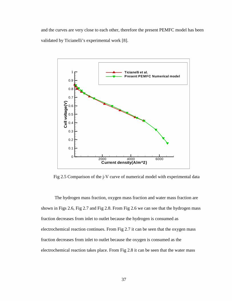
and the curves are very close to each other, therefore the present PEMFC model has been

validated by Ticianelli’s experimental work [8].

Fig 2.5 Comparison of the j-V curve of numerical model with experimental data

The hydrogen mass fraction, oxygen mass fraction and water mass fraction are

shown in Figs 2.6, Fig 2.7 and Fig 2.8. From Fig 2.6 we can see that the hydrogen mass

fraction decreases from inlet to outlet because the hydrogen is consumed as

electrochemical reaction continues. From Fig 2.7 it can be seen that the oxygen mass

fraction decreases from inlet to outlet because the oxygen is consumed as the

electrochemical reaction takes place. From Fig 2.8 it can be seen that the water mass

Current density(A/m^2)

Cel

lvol

tag

e(V

)

2000 4000 60000

0.1

0.2

0.3

0.4

0.5

0.6

0.7

0.8

0.9

1 Ticianelli et al.Present PEMFC Numerical model

38

fraction increases from inlet to outlet on the cathode side because water is produced from

the electrochemical reaction.

Fig 2.6 Hydrogen mass fraction at the anode side

Fig 2.7 Oxygen mass fraction at the cathode side

Fuel

Air

Fuel Air

39

Fig 2.8 Water mass fraction at the cathode side

Fuel

Air

40

CHAPTER 3

DESIGN OF UNIFORM FLOW BIPOLAR PLATE

In this chapter the baseline design of the bipolar plate is taken, and a numerical

analysis is carried out on it to study the velocity distributions. The flow distribution of the

bipolar plate is very important because, if the flow distribution is non-homogeneous there

will be a poor performance of the fuel cell and wastage of highly expensive catalyst. The

flow distribution of the baseline design is found to be non-homogeneous. The design of

the bipolar plate is changed to four inlets and four outlets so that the flow distribution

becomes more homogeneous.

3.1 Design Description

The baseline design of the PEMFC is shown in Fig 3.1. The model consists of

bipolar plates with thirteen channels each with one inlet and outlet. The whole model of

the PEMFC consists of nine parts: two gas channels, two bipolar plates, two gas diffusion

layers, two catalyst layers and a membrane. The parallel channel layout is implemented

for the channels of the bipolar plate. The header section is designed with rectangular

obstructions, so that the gases flow into the channels. The dimensions of the model are

shown in Fig 3.2. The CAD model was designed using the commercial software

SOLIDWORKS 2008®. The Initial Graphics Exchange Specification (IGES) file is

loaded into Hypermesh® software for meshing of the designed CAD model.

41

Fig 3.1 PEMFC baseline design

Fig 3.2 Dimensions of the baseline design of PEMFC (unit: mm)

Anode bipolar plate

Cathode bipolar plate

Anode Flow channels

Cathode Flow channels

Membrane

Cathode Catalyst

Anode Catalyst

Cathode GDL

Anode GDL

Fuel inlet

Air inlet

Fuel outlet

Fuel inlet

Fuel outlet

Air outlet

42

The designed baseline design of the PEMFC consists of two bipolar plates with

dimensions as shown in Fig 3.2. The thickness of the bipolar plate is 2 mm with 62 mm×

62 mm width and length. The channel width is 2 mm and the channel rib is 2 mm wide

and 1 mm in height. The rectangular obstruction in the header area is 2 mm× 0.5 mm × 1

mm. The inlet diameter is 4.5 mm. The thickness of the gas diffusion layers is 0.26 mm.

The thickness of membrane is 0.23 mm and the thickness of the catalyst layer is 0.01

mm. The gas diffusion layers, the catalyst layers and the membrane are 62 mm×62 mm

in width and length. The computational mesh is generated by using the powerful meshing

software Hypermesh ®. The generated mesh consists of 935,050 cells and 627,859 nodes

which is the optimized one. The computational mesh can be seen in Figs 3.3(a), (b), (c).

Hexahedral elements are used for the channels and tetrahedral elements are used at the

inlet and outlet of the bipolar plate.

Fig 3.3(a) Computational mesh of the PEMFC

43

Fig 3.3(b) Computational mesh of channels and the MEA

Fig 3.3(c) Mesh of bipolar plate and flow channels

44

3.2 Hydrodynamic Analysis

The commercial CFD software Fluent® is used as the computational tool for

numerical analysis. Only a hydrodynamic analysis with no heat transfer is carried out

on the above PEMFC and the electrochemical processes are not considered. The

PEMFC module in Fluent is not available, so only the hydrodynamic analysis is

carried out. The flow distributions in the bipolar plate are studied. The boundary

conditions are: (1) anode mass inlet: 6.0x10-7 kg/sec, (2) cathode mass inlet: 5.0x10-6

kg/sec and the inlet temperature is given as 50oC. The calculated result of flow

distribution can be found in Fig 3.4. Fig 3.4 shows that the flow distribution is not

uniform. The velocity is higher at the inlet and outlet and lower at the middle part of

the bipolar plate. The bar chart below shows the flow distribution in the bipolar plate

at the middle of the channel.

Fig 3.4 Flow distribution in the bipolar plate

45

The flow distribution in the baseline design of the bipolar plate is non-uniform

and this leads to the wastage of very expensive catalyst and also there will be a poor

performance of the fuel cell. The design of the bipolar plate should be changed, so that

the flow distribution is uniform. The design of the bipolar plate is changed with four

inlets and four outlets instead of one inlet and one outlet. The improved design of the

PEMFC can be seen in Fig 3.5. The dimensions of the PEMFC can be found in Fig 3.6.

Fig 3.5 Improved design of PEMFC

Anode bipolar plate

Cathode bipolar plate

Anode Flow channels

Cathode Flow channels

Membrane Cathode Catalyst

Anode Catalyst

Cathode GDL

Anode GDL

Fuel inlet

Air inlet

Fuel outlet

Air outlet

46

Fig 3.6 Dimensions of improved design PEMFC (unit: mm)

The dimensions can be seen clearly in Fig 3.6. The width of the bipolar plate is 60

mm and length 80 mm. There are four inlets and four outlets with 6 mm diameter each.

The header is designed with cylindrical obstructions which are 1.6 mm in diameter and 1

mm in height. The channels present in the bipolar plate are 2 mm in width and 1 mm in

height. The CAD model has been designed in the modeling software SOLIDWORKS

2008®. The IGES file was loaded into Hypermesh® software for meshing of the designed

CAD model. Three-dimensional computational mesh is generated using Hypermesh®

software. The computational mesh can be seen in Figs 3.7 (a), (b) and (c). The generated

mesh consists of 1,587,586 elements and 858,736 nodes which is the optimized one.

Hexahedral elements are used at the channels. Tetrahedral elements are used at the

header, inlets and outlets. The boundary conditions are the same as the baseline design.

47

Fig 3.7(a) Computational mesh of improved design PEMFC

Fig 3.7(b) Computational mesh of flow channels and the MEA

48

Fig 3.7(c) Mesh of bipolar plate and the channels

The CFD software Fluent® is used for numerical analysis of the PEMFC. Only

hydrodynamic analysis is carried out on the present model. The electrochemical

processes are not considered because the PEMFC module is not available in Fluent®

software. The flow distributions are investigated inside the bipolar plate. The flow

distributions inside the bipolar plate are seen in Fig 3.8. The flow distribution is almost

uniform in every channel. The uniform flow is favorable for the fuel cell performance.

The uniform flow distribution provides better adjustment of fuel supply which leads to

higher efficiency of the fuel cell. The uniform flow distribution gives a uniform

temperature distribution, uniform electrochemical reaction rate in catalyst layers, and

efficient usage of expensive catalyst.

49

Fig 3.8 Flow distribution inside the channels of the improved design of PEMFC

The flow distribution is very uniform in the channels of the bipolar plate. One of

the channels is taken to carry out the electrochemical analysis. COMSOL

MULTIPHYSICS 3.5a is used for electrochemical analysis. Due to the limitation on the

extensive memory requirement of COMSOL®, only a single channel shown in Fig 3.9 is

selected to simulate the behavior of the PEMFC. The same problem is faced by Xing et

al. [34], and the same thing was done by them. The half of the single channel of the

improved design PEMFC is taken and run as a symmetric model and the electrochemical

analysis is carried out. Fig 3.10 shows the temperature distribution along the cathode gas

channel. Fig 3.11 shows the temperature distribution along the anode gas channel. From

Figs 3.10 and 3.11 we can observe that the outlet temperature at cathode is more than that

of the anode because the electrochemical reaction produces exothermic heat which is

absorbed by the air at the cathode side. The heat from the cathode is absorbed by the

anode also by conduction.

50

Fig 3.9 Computational domain

Fig 3.10 Temperature distribution along the cathode gas channel

Elements: 2260 Nodes: 3312 Type: Hexahedral

Fuel velocity = 3.337 m/s Air velocity = 2.181 m/s Fuel and air inlet temperature = 323 K

51

Fig 3.11 Temperature distribution along the anode gas channel

3.3 Electrochemical Analysis

The electrochemical analysis is carried out using COMSOL MULTIPHYSICS

3.5a software and the mass fractions of hydrogen, oxygen and water at the anode and

cathode are shown in Figs 3.12, 3.13and 3.14. From Fig 3.12 we can observe that the

hydrogen mass fraction decreases from inlet to outlet at the anode channel. From Fig 3.13

it is seen that the oxygen mass fraction is decreased from inlet to outlet at the cathode

channel. From Fig 3.14 it can be seen that the water mass fraction increases from inlet to

outlet.

The mass fraction of hydrogen decreases from inlet to the outlet because

hydrogen is consumed by the electrochemical reaction along the length of the channel.

The mass fraction of oxygen decreases from inlet to outlet because the oxygen is used up

by the electrochemical reaction to produce electricity. The water mass fraction increases

from inlet to the outlet because the hydrogen and oxygen ions combine and form by-

product water which is produced at the cathode channel of the PEMFC.

Fuel velocity = 3.337 m/s Air velocity = 2.181 m/s Fuel and air inlet temperature = 323 K

52

Fig 3.12 Hydrogen mass fraction at the anode channel

Fig 3.13 Oxygen mass fraction at the cathode gas channel

Fuel

Air

Fuel

Air

Fuel

Air

53

Fig 3.14 Water mass fraction at the cathode gas channel

Fuel

Air

54

CHAPTER 4

OPTIMIZATION OF PEMFC CHANNEL GEOMETRY

In this chapter the geometry of the channel is changed from rectangular to square,

semi-circle and triangle, and the performances are determined. From the obtained

numerical results it is seen that the rectangular geometry is better than all of the

geometries. The triangular channel has the poorest performance of all the four channel

geometries. The numerical results for different geometries are found for various

temperatures and pressures.

4.1 Design Description

The geometry of the channel has been changed to different shapes. The shape of

the channel designed in Chapter 3 is rectangular. The shape of the channel is changed

from rectangular to square, semi-circle and triangular shapes. The shapes of the channels

can be seen in Figs 4.1, 4.2, 4.3 and 4.4. The width of the rectangular channel is 2 mm

and height is 1 mm.

Fig 4.1 Rectangular channel

Anode current collector

Cathode current collector

Membrane

Cathode catalyst layer

Cathode GDL

Anode GDL

Anode catalyst layer

Anode Flow channel

Cathode Flow channel

55

Fig 4.2 Square channel

Fig 4.3 Semi-circular channel

1.4 mm

1.4 mm

1 mm

56

Fig 4.4 Triangular channel 4.2 Numerical Analysis

The COMSOL MULTIPHYSICS 3.5a is used for electrochemical analysis of all

the channel geometries. The parameters and boundary conditions stated in Chapter 2 are

used for the numerical analysis. The rectangular, square, semi-circular and triangular

channels are numerically simulated and a j-V curve is plotted for each. The j-V curves

can be seen in Fig 4.5. From Fig 4.5 it can be observed that rectangular channel shows

better performance than that of every other channel. The performance of the rectangular

is 6.3% greater than the triangular channel.

1.5 mm 1.5 mm

1.5 mm

57

Fig 4.5 j-V curves of different channel geometries

The reason for the above behavior may be due to the area surrounding the

channel. The area surrounding the channel is determined and compared with the

performance. The area of the solid surface in contact with the fluid flow influences the

performance of the fuel cell. The larger the area the higher is the performance. The total

channel surface areas are: rectangular channel 240 mm2, square channel 224 mm2, semi-

circular channel 205.6 mm2, triangular channel 180 mm2. The rectangular channel has the

larger area when compared with other channels, so the performance of the rectangular

channel is better than all the channels. The current produced is directly proportional to

Current density(A/m^2)

Cel

lvol

tage

(V)

2000 4000 6000 80000

0.2

0.4

0.6

0.8

1

RectangularSquareSemi-circularTriangular

58

the area of interface [2]. Doubling the interfacial area available for the reaction should

double the rate of the reaction. The large area has better reaction rate, so there is an

increase in performance when the area is increased. The current density (current per unit

area) is more fundamental than current. The current density allows the reactivity of

different surfaces to be compared on a per-unit basis. Current density � is expressed in

units of amperes per square centimeter (A/m2):

� �&

= (4-1)

where A is the area and ( is the current (A)

In a similar fashion, the electrochemical reaction rates are also expressed on a per-

unit area basis. The per-unit area reaction rate is given the symbol >. Area-normalized

reaction rates are usually expressed in units of moles per square centimeter per time

(mol/cm2/s):

> ��

=

?@

?��

&

��=�

-

�� (4-2)

where F is the Faraday’s constant , A is the area and � is the number of moles of

electrons transferred during the electrochemical reaction. The above equations show the

importance of the area. The larger area is better for reactions. The main parameter,

current density, is related to area. Fig 4.6 shows the power density curves of different

channel geometries. The power density curves show that the maximum power is obtained

at a voltage of 0.6 V. The power density obtained from the rectangular channel is better

than all the channels.

59

Fig 4.6 Power density curves of different channel geometries

4.3 Pressure Drop Calculation

The pressure drop is very important in the design of channels. The pressure

difference between the inlet and outlet drives the fluid flow. Increasing the pressure drop

between the inlet and outlet will increase the mean gas velocity in the channel, improving

convection. The pressure drop is calculated analytically for different channels and

compared with the numerical results obtained. For circular flow channels, the

relationship between pressure drop and mean gas velocity may be calculated from the

relation [2]

?A

?B�

C

DEF (4-3)

where :G :H⁄ is the pressure gradient, D is the flow channel diameter, and the mean wall

shear stress EF may be calculated from a nondimensionalized number called the friction

factor,I [2]:

C e ll vo lta g e ( V )

Pow

erd

ensi

ty(

W/m

2̂)

0 .2 0 .3 0 .4 0 .5 0 .6 0 .7 0 .8 0 .9

5 0 0

1 0 0 0

1 5 0 0

2 0 0 0

2 5 0 0

3 0 0 0

R e cta n g u la rS q u a reS e m i-c irc u la rT ria n g u la r

60

I �JK

� LMNO⁄ (4-4)

where P is the fluid density �QR ST�⁄ and U is the mean flow velocity (m/s). It is found

that regardless of channel size or flow velocity, IRe = 16 for laminar flow in circular

channels. Furthermore, for circular channels [2]

) �MND

V (4-5)

Thus, by combining equations (4-3), (4-4) and (4-5) and the fact that IRe = 16,

the pressure drop and mean gas velocity may be related:

?A

?B�

TLN

DO (4-6)

Unfortunately, most fuel cell flow channels are rectangular instead of circular. For

rectangular channels equation (4-6) cannot be used. For rectangular channels, we must

use hydraulic diameter to compute the effective Reynolds number compared to a circular

channel [2]:

)$ �MNDW

V (4-7)

where

2$ � C=

��

CX�Y#ZZ�Z*��&#��+ �Y*�

A*Y&%*�*Y (4-8)

For rectangular channels, the relationship between )$, and I is more complex than for

circular channels. It can be approximated as [35]:

I)$ � 24�1 � 1.355_� � 1.9467_�O� 1.7012_�d

� 0.9564_�e� 0.2537_�f

� (4-9)

where _� is the aspect ratio of the channel cross section: _� � � �⁄ , where 2 � and 2 �

are the lengths of the channel sides. The aspect ratio _� for different channel geometries

can be obtained as shown in Fig 4.7.

61

Rectangle Square

Semi-circle Triangle Fig 4.7 Aspect ratio calculation for different geometries

a

b

a

b

a

b

a

b

62

The pressure drop in the channels is calculated analytically and compared with the

numerical results in Table 4.1. The numerical results approached the analytical value with

less than 5% error. The analytical calculations are carried out considering the flow in the

channel as fully developed, so the numerical results are overestimated compared to

analytical values.

Fig 4.8 Velocity vector plot in the gas channel

Fig 4.8 shows that the flow inside the channel is not fully developed. The

developing lengths on the anode side and cathode side are found to be 39.29 mm and

37.89 mm. The length of the channel should be increased to a length greater than the

developing length.

63

Table 4.1 Pressure drop comparison

Type of geometry

Pressure drop (Pa)

Analytical value

Numerical results

Error (%)

Rectangular Square Semi-circle Triangle

132.3 107.04 145.68 155.42

138.65 111.62 151.36 162.63

4.58 4.10 3.75 4.43

4.4 Temperature Variation

The operating temperature is changed from 323K to 338K and 353K and the

performance of the fuel cell is observed. The pressure on the cathode and anode side is 1

atm. The performance of the fuel cell increases with increase in temperature. The reason

behind this nature is that the kinetic performance focuses on increasing j0 (exchange

current density). To understand how j0 is increased we have to take a look how j0 is

defined. The j0 is defined by the equation (4-8) [2].

�� � �1g��I��∆ij ����⁄ (4-8)

where �� is the exchange current density, F is Faraday’s constant, � is the number of

moles of electrons, g�� is the reactant concentration, ∆k� is the activation barrier and T is

the temperature.

64

From the above equation we can observe that by increasing the temperature the

exchange current density can be increased, and thereby increasing the performance of the

fuel cell. By increasing the reaction temperature, we are increasing the thermal energy

available in the system. When the thermal energy in the system is increased all particles

in the system move about and vibrate with increased intensity. The higher level of

thermal activity increases the likelihood that given reactants will posses sufficient energy

to reach the activated state, thus increasing the rate of reaction [2]. Changing the

temperature has an exponential effect on ��. The j-V curves for the various channel

geometries at different temperatures are presented in Figs 4.9, 4.11, 4.13 and 4.15. The

power density curves are presented in Figs 4.10, 4.12, 4.14, 4.16.

Fig 4.9 j-V curves of the rectangular channel at different temperatures

C u rre n t d e n s ity ( A /m ^ 2 )

Cel

lvo

ltag

e(V

)

1 0 0 0 2 0 0 0 3 0 0 0 4 0 0 0 5 0 0 0 6 0 0 0 7 0 0 00

0 .1

0 .2

0 .3

0 .4

0 .5

0 .6

0 .7

0 .8

0 .9

1R e c ta n g le ( 3 5 3 K )R e c ta n g le ( 3 3 8 K )R e c ta n g le ( 3 2 3 K )Fuel velocity = 3.337 m/s

Air velocity = 2.181 m/s

65

Fig 4.10 Power density curves of the rectangular channel at different temperatures

Fig 4.11 j-V curves of the square channel at different temperatures

C e ll v o lta g e ( V )

Pow

erd

ensi

ty(A

/m^2

)

0 .2 0 .3 0 .4 0 .5 0 .6 0 .7 0 .8 0 .9

5 0 0

1 0 0 0

1 5 0 0

2 0 0 0

2 5 0 0

3 0 0 0

R e c ta n g le ( 3 5 3 K )R e c ta n g le ( 3 3 8 K )R e c ta n g le ( 3 2 3 K )

C u rre n t d e n s ity ( A /m ^ 2 )

Cel

lvo

ltag

e(V

)

1 0 0 0 2 0 0 0 3 0 0 0 4 0 0 0 5 0 0 0 6 0 0 0 7 0 0 00

0 .1

0 .2

0 .3

0 .4

0 .5

0 .6

0 .7

0 .8

0 .9

1 S q u a re ( 3 5 3 K )S q u a re ( 3 3 8 K )S q u a re ( 3 2 3 K )

Fuel velocity = 3.337 m/s Air velocity = 2.181 m/s

Fuel velocity = 3.405 m/s Air velocity = 2.225 m/s

66

Fig 4.12 Power density curves of the square channel at different temperatures

Fig 4.13 j-V curves of the semi-circular channel at different temperatures

C e l l v o l t a g e ( V )

Po

wer

des

ity(

W/m

^2)

0 . 2 0 . 3 0 . 4 0 . 5 0 . 6 0 . 7 0 . 8 0 . 9

5 0 0

1 0 0 0

1 5 0 0

2 0 0 0

2 5 0 0

3 0 0 0

S q u a r e ( 3 5 3 K )S q u a r e ( 3 3 8 K )S q u a r e ( 3 2 3 K )

C u r r e n t d e n s it y ( A / m ^ 2 )

Cel

lVol

tage

(V)

1 0 0 0 2 0 0 0 3 0 0 0 4 0 0 0 5 0 0 0 6 0 0 0 7 0 0 00

0 .1

0 .2

0 .3

0 .4

0 .5

0 .6

0 .7

0 .8

0 .9

1S e m i- c ir c le ( 3 5 3 K )S e m i- c ir c le ( 3 3 8 K )S e m i- c ir c le ( 3 2 3 K )

Fuel velocity = 3.405 m/s Air velocity = 2.225 m/s

Fuel velocity = 3.725 m/s Air velocity = 2.578 m/s

67

Fig 4.14 Power density curves of the semi-circular channel at different temperatures

Fig 4.15 j-V curves of the triangular channel at different temperatures

C e ll v o lta g e ( V )

Pow

erde

nsi

ty(

W/m

^2)

0 .2 0 .3 0 .4 0 .5 0 .6 0 .7 0 .8 0 .9

5 0 0

1 0 0 0

1 5 0 0

2 0 0 0

2 5 0 0

3 0 0 0

S e m i- c irc le ( 3 5 3 K )S e m i- c irc le ( 3 3 8 K )S e m i- c irc le ( 3 2 3 K )

C u r r e n t d e n s it y ( A / m ^ 2 )

Cel

lvo

ltag

e(V

)

1 0 0 0 2 0 0 0 3 0 0 0 4 0 0 0 5 0 0 0 6 0 0 0 7 0 0 00

0 .1

0 .2

0 .3

0 .4

0 .5

0 .6

0 .7

0 .8

0 .9

1 T r ia n g le ( 3 5 3 K )T r ia n g le ( 3 3 8 K )T r ia n g le ( 3 2 3 K )

Fuel velocity = 3.725 m/s Air velocity = 2.578 m/s

Fuel velocity = 4.235 m/s Air velocity = 2.773 m/s

68

Fig 4.16 Power density curves of the triangular channel at different temperatures

From the above Figs 4.9, 4.11, 4.13 and 4.15 we can observe that the slope of the

j-V curve changes with variation of temperature at the activation region. The slope of the

j-V curve doesn’t change in the ohmic region and in the concentration region. This is

because increase in temperature influences only the activation as explained above and

doesn’t influence the ohmic and concentration regions of the j-V curve. The slopes of the

above j-V curves are tabulated in Table 4.2. The solid line in Figs 4.9, 4.11, 4.13 and 4.15

represents the j-V curve at 353K (800C), the dashed line in Figs 4.9, 4.11, 4.13 and 4.15

represents the j-V curve at 338K (650C) and the dashed dot line in Figs 4.9, 4.11, 4.13

and 4.15 represents the j-V curve at 323K (500C).

c e ll v o lta g e ( V )

Pow

erde

nsity

(W

/m^2

)

0 .2 0 .3 0 .4 0 .5 0 .6 0 .7 0 .8 0 .9

5 0 0

1 0 0 0

1 5 0 0

2 0 0 0

2 5 0 0

3 0 0 0T ria n g le ( 3 5 3 K )T rin a g le ( 3 3 8 K )T ria n g le ( 3 2 3 K )

Fuel velocity = 4.235 m/s Air velocity = 2.773 m/s

69

Table 4.2 Slopes of the j-V curves at different temperatures

Shape of the channel

Temperatures (1)353K, (2)338K and (3)323K Slope

Activation region (400 – 1000 A/m2)

Ohmic region (2000 – 4200 A/m2)

Concentration region (5500 – 6400 A/m2)

Rectangle

1 6e-5 7.143e-5 1.92e-4

2 8e-5 7.143e-5 1.958e-4

3 10e-5 7.143e-5 2e-4

Square

1 6.315e-5 6.514e-5 1.75e-4

2 8.42e-5 6.514e-5 1.78e-4

3 10.53e-5 6.514e-5 1.792e-4

Semi-circle

1 6.67e-5 5.83e-5 1.555e-4

2 9.167e-5 5.83e-5 1.583e-4

3 11.67e-5 5.83e-5 1.61e-4

Triangle

1 7.5e-5 5.435e-5 1.52e-4

2 10e-5 5.435e-5 1.532e-4

3 13.33e-5 5.435e-5 1.553e-4

70

From Table 4.2 it can be observed that the value of the slopes remains constant in

the ohmic region but the slopes change drastically in the activation region. The less the

slope the better is the performance. Increasing the temperature decreases the activation

loss and therefore decreasing the slope of the j-V curve at the activation region.

4.5 Pressure Variation

The operating pressures of the fuel cell are varied from 1 atm on both anode and

cathode sides to 2 atm on the anode side and 4 atm on the cathode side, and the j-V

curves are calculated to check the performance of the fuel cell. The operating pressure is

again changed from 2 atm and 4 atm at the anode and cathode side to 3 atm and 5 atm at

the cathode side. Figs 4.17, 4.19, 4.21 and 4.23 represent the j-V curves of the different

channel geometries at different operating pressures. Figs 4.18, 4.20, 4.22 and 4.24

represent the power density curves of different channel geometries at different operating

pressures.

Fig 4.17 j-V curves of the rectangular channel at various operating pressures

C u r r e n t d e n s i t y ( A / m ^ 2 )

Cel

lvo

ltag

e(V

)

1 0 0 0 2 0 0 0 3 0 0 0 4 0 0 0 5 0 0 0 6 0 0 0 7 0 0 00

0 .1

0 .2

0 .3

0 .4

0 .5

0 .6

0 .7

0 .8

0 .9

1 R e c t a n g le ( A :3 a t m / C :5 a t m )R e c t a n g le ( A :2 a t m / C :4 a t m )R e c t a n g le ( A :1 a t m / C :1 a t m )

Fuel velocity = 3.337 m/s Air velocity = 2.181 m/s

71

Fig 4.18 Power density curves of the rectangular channel at various operating pressures

Fig 4.19 j-V curves of the square channel at various operating pressures

C e ll v o lta g e ( V )

Pow

erde

nsity

(W

/m^2

)

0 .2 0 .3 0 .4 0 .5 0 .6 0 . 7 0 .8 0 .9

5 0 0

1 0 0 0

1 5 0 0

2 0 0 0

2 5 0 0

3 0 0 0

R e c ta n g le ( A : 3 a tm /C : 5 a tm )R e c ta n g le ( A : 2 a tm / C : 4 a tm )R e c ta n g le ( A : 1 a tm / C : 1 a tm )

C u rre n t d e n s ity ( A /m ^ 2 )

Cel

lvo

ltag

e(V

)

1 0 0 0 2 0 0 0 3 0 0 0 4 0 0 0 5 0 0 0 6 0 0 0 7 0 0 00

0 .1

0 .2

0 .3

0 .4

0 .5

0 .6

0 .7

0 .8

0 .9

1S q u a re ( A :3 a tm / C :5 a tm )S q u a re ( A :2 a tm / C :4 a tm )S q u a re ( A :1 a tm / C :1 a tm )

Fuel velocity = 3.337 m/s Air velocity = 2.181 m/s

Fuel velocity = 3.405 m/s Air velocity = 2.225 m/s

72

Fig 4.20 Power density curves of the square channel at various operating pressures

Fig 4.21 j-V curves of the semi-circular channel at various operating pressures

C e ll v o lta g e ( V )

Pow

erde

nsi

ty(

W/m

^2)

0 .2 0 .3 0 .4 0 .5 0 .6 0 .7 0 .8 0 .9

5 0 0

1 0 0 0

1 5 0 0

2 0 0 0

2 5 0 0

3 0 0 0

S q u a re ( A : 3 a tm / C : 5 a tm )S q u a re ( A : 2 a tm / C : 4 a tm )S q u a re ( A : 1 a tm / C : 1 a tm )

C u rre n t d e n s ity ( A / m ^ 2 )

Cel

lvo

ltag

e(V

)

1 0 0 0 2 0 0 0 3 0 0 0 4 0 0 0 5 0 0 0 6 0 0 0 7 0 0 00

0 .1

0 .2

0 .3

0 .4

0 .5

0 .6

0 .7

0 .8

0 .9

1S e m i- c irc le ( A :3 a tm / C :5 a tm )S e m i- c irc le ( A :2 a tm / C :4 a tm )S e m i- c irc le ( A :1 a tm / C :1 a tm )

Fuel velocity = 3.405 m/s Air velocity = 2.225 m/s

Fuel velocity = 3.725 m/s Air velocity = 2.578 m/s

73

Fig 4.22 Power density curves of the semi-circular channel at various operating pressures

Fig 4.23 j-V curves of the triangular channel at various operating pressures

C e ll v o lta g e ( V )

Pow

erde

nsi

ty(

W/m

^2)

0 .2 0 .3 0 .4 0 .5 0 .6 0 .7 0 .8 0 .9

5 0 0

1 0 0 0

1 5 0 0

2 0 0 0

2 5 0 0

3 0 0 0

S e m i- c irc le ( A : 3 a tm / C : 5 a tm )S e m i- c irc le ( A : 2 a tm / C : 4 a tm )S e m i- c irc le ( A : 1 a tm / C : 1 a tm )

C u rre n t d e n s ity ( A /m ^ 2 )

Cel

lvo

ltag

e(V

)

1 0 0 0 2 0 0 0 3 0 0 0 4 0 0 0 5 0 0 0 6 0 0 0 7 0 0 00

0 .1

0 .2

0 .3

0 .4

0 .5

0 .6

0 .7

0 .8

0 .9

1T r ia n g le ( A :3 a tm / C :5 a tm )T r ia n g le ( A :2 a tm / C :4 a tm )T r ia n g le ( A :1 a tm / C :1 a tm )

Fuel velocity = 3.725 m/s Air velocity = 2.578 m/s

Fuel velocity = 4.235 m/s Air velocity = 2.773 m/s

74

Fig 4.24 Power density curves of the triangular channel at various operating pressures

Increasing the pressure has less effect on the performance of the fuel cell when

compared with increasing temperature. The solid line in Figs 4.17, 4.19, 4.21 and 4.23

represents the j-V curve of the fuel cell at an operating pressure of 3 atm on the anode

side and 5 atm on the cathode side. The dashed line Figs 4.17, 4.19, 4.21 and 4.23

represents the j-V curve of the fuel cell at an operating pressure of 2 atm on the anode

side and 4 atm on the cathode side. The dashed dot line in Figs 4.17, 4.19, 4.21 and 4.23

represents the j-V curve of the fuel cell at an operating pressure of 1 atm at both the

anode and cathode side. From Figs 4.17, 4.19, 4.21 and 4.23 it can be observed that the

performance increases with increasing the operating pressure. The slopes of the j-V

curves are tabulated in Table 4.3.

Table 4.3 Slopes of the j-V curves at different operating pressures

C e ll v o lta g e ( V )

Pow

erd

ensi

ty(

W/m

2̂)

0 .2 0 .3 0 .4 0 .5 0 .6 0 .7 0 .8 0 .9

5 0 0

1 0 0 0

1 5 0 0

2 0 0 0

2 5 0 0

T r ia n g le ( A : 3 a tm /C : 5 a tm )T r ia n g le ( A : 2 a tm /C : 4 a tm )T r ia n g le ( A : 1 a tm /C : 1 a tm )

Fuel velocity = 4.235 m/s Air velocity = 2.773 m/s

75

Shape of the channel

Pressures (1.A: 3atm/C: 5atm), (2.A: 2atm/C: 4atm) and (3.A: 1atm/C: 1atm) Slope

Activation region (400 – 1000 A/m2)

Ohmic region (2000 – 4200 A/m2)

Concentration region (5500 – 6400 A/m2)

Rectangle

1 8e-5 5.88e-5 1.23e-4

2 8.25e-5 5.88e-5 1.535e-4

3 8.45e-5 5.88e-5 1.78e-4

Square

1 9.375e-5 6.38e-5 1.18e-4

2 9.436e-5 6.38e-5 1.35e-4

3 9.532e-5 6.38e-5 1.462e-4

Semi-circle

1 10.05e-5 7.1e-5 1.15e-4

2 10.22e-5 7.1e-5 1.362e-4

3 10.35e-5 7.1e-5 1.523e-4

Triangle

1 11.23e-5 7.567e-5 1.083e-4

2 11.375e-5 7.567e-5 1.253e-4

3 11.489e-5 7.567e-5 1.476e-4

From Table 4.3 we can observe that slopes at the ohmic region remain the same

and the slopes at the concentration region changes. The slope of the j-V curves decreases

with increase in pressure. The less the slope the better is the performance. The

concentration loss is decreased when the pressure is increased, so there is change in the

76

slope of the j-V curve at the concentration region. The performance of the fuel cell may

be increased due to better supply of reactants at higher pressures to active sites near the

front surface of the electrodes, which is the predominant reaction zone at higher current

densities [8].

77

CHAPTER 5

CONCLUSIONS AND RECOMMENDATIONS

5.1 Conclusions

A single channel PEMFC is taken and validated by comparing the numerical

results with the published experimental data in the literature. The obtained results are in

good agreement with the available published experimental data. The validated parameters

are then applied to the future designs. An improved design of the bipolar plate is

developed for uniform flow. The flow channel geometry is changed to different shapes

and the performance is observed. The conclusions pertaining to this research work are

summarized as follows:

• Uniform flow distribution is obtained in the improved design of the bipolar plate.

The baseline design has non-uniform flow distribution, the velocity high at the

lateral channels and low at the center channels.

• The geometry of the channel is changed from the rectangular shape to square,

semi-circle and triangular shapes and the performance of the fuel cell is observed.

The rectangular channel has better performance when compared with the other

channels. The reason for this may be due to the area that is in contact with the

fluid flow. The triangular channel has the worst performance when compared with

other channels.

• The operating temperature of the fuel cell is varied and the performance is

observed. The performance of the fuel cell increases with increase in temperature.

This is because as the temperature is increased the exchange current density is

increased therefore increasing the performance of the fuel cell. Increasing the

78

reaction temperature increases the thermal energy available in the system and all

the molecules in the system move about and vibrate with increased intensity

increasing the rate of the reaction.

• The operating pressure of the fuel cell is varied and the resulting performance is

observed. The performance of the fuel cell increases with increase in operating

pressure. The increase in performance is very little when the pressure is increased.

The increase in performance may be because of a better supply of reactants at

higher pressures.

5.2 Recommendations

The electrochemical analysis is carried out using the COMSOL® software and due

to the limitation on extensive memory requirement of COMSOL® only a single channel is

selected to simulate the behavior of the PEMFC. Fuel cell module in Fluent can be used

for detailed study of the PEMFC with huge number of elements, so that more accurate

results can be obtained. If the fuel cell module in Fluent® is available a single PEMFC or

a stack can be numerically analyzed. The change in the flow channel geometry should be

studied in more detail. The performance of the whole fuel cell may be different from the

single channel analysis. No experimental work has been done on the current design of the

geometries of the channels. The experimental results can be used to validate the

numerical simulations performed. A real time experiment may be carried out to know the

exact behavior of each and every component of the fuel cell. The start up and shut down

processes involved in the PEMFC can be studied. The flow in the channel is not fully

developed. This led to overestimation of the numerical results when compared to

79

analytical results. The flow in the channel is not fully developed because the length of the

channel is less than the developing length of the flow. The length of the channel should

be increased to a length greater than the developing length to obtain fully developed flow

in the channel.

80

REFERENCES

1. www.fuelcells.org

2. Ryan. O’Hayre, Suk-Won Cha, Whitney Colella, Fritz B. Prinz “Fuel cell

fundamentals (2009)”, John Wiley & sons, Inc, ISBN 9780470258439, 2nd edition,

2009

3. http://inventors.about.com/od/fstartinventions/a/Fuel_Cells.htm

4. http://americanhistory.si.edu/fuelcells/

5. D.M. Bernardi, M.W. Verbrugge, “A mathematical model of the solid polymer-

electrolyte fuel cell,” Journal of Electrochemical Society 139 (9) (1992) 2477–2491.

6. S. Dutta, S. Shimpalee, J.W.Van Zee, “Three-dimensional numerical simulation of

straight channel PEM fuel cells,” Journal of Applied Electrochemistry. 30 (2000)

135–146

7. T. Berning, D.M. Lu, N. Djilali, “Three-dimensional computational analysis of

transport phenomena in a PEM fuel cell,” Journal of Power Sources 106 (2002) 284–

294.

8. E.A. Ticianelli, C.R. Derouin, A. Redondo and S. Srinivasan, “Methods to Advance

Technology of Proton Exchange Membrane Fuel Cells,” J. Electrochm. Soc. 135 (9)

(1988) 2209–2214.

9. P.C. Sui, S. Kumarb, N. Djilali “Advanced computational tools for PEM fuel cell

design Part 1. Development and base case simulations,” Journal of Power Sources

180 (2008) 410–422

81

10. P.C. Sui, S. Kumarb, N. Djilali “Advanced computational tools for PEM fuel cell

design Part 2. Development and base case simulations,” Journal of Power Sources

180 (2008) 423–432

11. R.F. Mann, J.C. Amphlett, M.A.I. H.M. Hooper, Jensen, B.A. Peppley, P.R.

Roberge, “Development and application of a generalized steady-state

electrochemical model for a PEM fuel cell,” Journal of Power Sources, 86, pp. 173-

180, 2000.

12. P.T. Nguyen, T. Berning, Djilali, “Computational model of a PEM fuel cell with

serpentine gas flow channels,” Journal of Power Sources, 130, pp. 149-157, 2004

13. S.Dutta , Sirivatch Shimpalee , J.W. Van Zee ” Numerical prediction of mass-

exchange between cathode and anode channels in a PEM fuel cell,” International

Journal of Heat and Mass Transfer 44 (2001) 2029-2042.

14. A.Kazim, H.T. Liu and P. Forges “Modelling of performance of PEM fuel cells with

conventional and interdigitated flow fields,” Journal of Applied Electrochemistry 29:

1409 -1416, 1999.

15. J. Park, X. Li, “An experimental and numerical investigation on the cross flow

through gas diffusion layer in a PEM fuel cell with a serpentine flow channel,”

Journal of Power Sources, 163, pp. 853- 863, 2007.

16. S.A. Grigoriev, A.A. Kalinnikov, V.N. Fateev, A.A. Wragg, “Numerical

optimization of bipolar plates and gas diffusion layers for PEM fuel cells,” Journal

of Applied Electrochemistry, 36, pp. 991-996, 2006.

17. J. Wind, R. Spah, W. Kaiser, G. Bohm “Metallic bipolar plates for PEM fuel cells,”

Journal of Power Sources 105 (2002) 256–260.

82

18. E.A. Cho, U.S. Jeon, H.Y. Ha, S.A. Hong, I.H. Oh, “Characteristics of composite

bipolar plates for polymer electrolyte membrane fuel cells,” Journal of Power

Sources, 125, pp. 178-182, 2004.

19. E. Sgrecciaa,d, M.L. Di Vona, S. Licoccia, M. Sganappa, M. Casciola, J.F. Chailan,

P. Knauth “Self-assembled nanocomposite organic–inorganic proton conducting

sulfonated poly-ether-ether-ketone (SPEEK)-based membranes: Optimized

mechanical, thermal and electrical properties,” Journal of Power Sources 192 (2009)

353–359.

20. Qiangu Yan , Hossein Toghiani , Junxiao Wu “Investigation of water transport

through membrane in a PEM fuel cell by water balance experiments”, Journal of

Power Sources 158 (2006) 316–325.

21. Beuscher U., Cleghorn S.J.C., Johnson W.B., “Challenges for PEM fuel cell

membranes”, International Journal of Energy Research, 29 (12), 1103-1112, 2005

22. L. Cindrella , A.M. Kannan, J.F. Lin, K. Saminathan, Y. Ho, C.W. Lin, J. Wertz

“Gas diffusion layer for proton exchange membrane fuel cells—A review,” Journal

of Power Sources 194 (2009) 146–160.

23. Xiao-Dong Niu, Toshihisa Munekata , Shi-Aki Hyodo, Kazuhiko Suga “An

investigation of water-gas transport processes in the gas-diffusion-layer of a PEM

fuel cell by a multiphase multiple-relaxation-time lattice Boltzmann model,” Journal

of Power Sources 172 (2007) 542–552.

24. Jay Benziger , James Nehlsen, David Blackwell, Tom Brennan, Johannah Itescu

“Water flow in the gas diffusion layer of PEM fuel cells” Journal of Membrane

Science 261 (2005) 98–106.

83

25. Shengsheng Zhang, Xiao-Zi Yuan, Jason Ng Cheng Hin, HaijiangWang, K.Andreas

Friedrich, Mathias Schulze. “A review of platinum-based catalyst layer degradation

in proton exchange membrane fuel cells” Journal of Power Sources 194 (2009) 588–

600

26. Feng-Yuan Zhang, Suresh G. Advani, Ajay K. Prasad, Mary E. Boggs, Shawn P.

Sullivan, Thomas P. Beebe Jr. “Quantitative characterization of catalyst layer

degradation in PEM fuel cells by X-ray photoelectron spectroscopy,”

Electrochimica Acta 54 (2009) 4025–4030.

27. Prodip K. Das, Xianguo Li , Zhong-Sheng Liu “A three-dimensional agglomerate

model for the cathode catalyst layer of PEM fuel cells,” Journal of Power Sources

179 (2008) 186–199.

28. Nawaz Akhtar, Arshad Qureshi, Joachim Scholta, Christoph Hartnig, Matthias

Messerschmidt, Werner Lehnert. “Investigation of water droplet kinetics and

optimization of channel geometry for PEM fuel cell cathodes” International Journal

of Hydrogen Energy 34 (2009) 3104-3111.

29. J.K. Kuo, C.K. Chen, “A novel Nylon-6-S316L fiber compound material for

injection molded PEM fuel cell bipolar plates,” Journal of Power Sources, 162 (1),

pp. 207-214, 2006.

30. Xiao-DongWang, Yuan-Yuan Duan,Wei-Mon Yan, Xiao-Feng Peng, “Effects of

flow channel geometry on cell performance for PEM fuel cells with parallel and

interdigitated flow fields,” Electrochimica Acta 53 (2008) 5334–5343

31. COMSOL MULTI-PHYSICS user guide

84

32. T.A. Zawodzinski, T.E. Springer, S. Gottesfeld, “Polymer electrolyte fuel cell

model,” Journal of the Electrochemical Society, v 138, n 8, Aug, 1991, p 2334-2342.

33. R.B. Bird, W.E. Stewart, and E.N. Lightfoot, Transport Phenomena, 2nd Edition,

John Wiley & Sons, Inc., 2002.

34. Xiu Qing Xing, KahWai Lum, Hee Joo Poh, Yan LingWu “Geometry optimization

for proton-exchange membrane fuel cells with sequential quadratic programming

method” , Journal of Power Sources 186 (2009) 10–21.

35. R.K shah and A.L London. Laminar flow forced convection in supplement 1 to

Advances in Heat Transfer, T.F. Irvine and J.P. Harnett (Eds.). Academic, New

York, 1978.

85

VITA

Graduate College University of Nevada, Las Vegas

Jephanya Kasukurthi

Degrees: Bachelor of technology, Mechanical Engineering, 2007 Acharya Nagarjuna University, India Selected publications:

[1] Jephanya Kasukurthi, K.M.Veepuri, J.H.Nie, Y.T. Chen, “Numerical Modeling of Velocity and Temperature Distributions in a Bipolar Plate of PEM Electrolysis Cell with Greatly Improved Flow Uniformity” ASME International Mechanical Engineering Congress and Exposition (IMECE2009-10519), November 13-19, 2009, Lake Buena Vista, Florida, USA

Thesis Title: Optimization of Channel Geometry in a PEM Fuel Cell

Thesis Examination Committee: Chairperson, Yitung Chen, Ph. D. Committee Member, Robert Boehm, Ph. D. Committee Member, Jianhu Nie, Ph. D. Graduate College Representative, Yahia Bagzhouz, Ph. D.