UNIVERSITY OF NAIROBI

SCHOOL OF ENGINEERING

DEPARTMENT OF ENVIRONMENTAL AND BIOSYSTEMS ENGINEERING

OPTIMIZATION OF BIOGAS PRODUCTION FROM BREWERY WASTEWATER

By

MURUNGA SYLVIA INJETE REECE

B TECH (Chem Eng, Moi U, 2007); MSc. (EBE, UoN, 2012)

Thesis submitted in partial fulfilment for the award of the Degree of Doctor of

Philosophy in Environmental and Biosystems Engineering of University of Nairobi

2017

i

DECLARATION

I declare that this is my original work and has not been presented for a degree in any other

University.

Name: Murunga Injete Reece Sylvia

Signature: Date:

This Thesis is submitted with our approval as university supervisors:

SUPERVISORS:

Name: Duncan Onyango Mbuge, PhD, UoN

Signature: Date:

Name: Ayub Njoroge Gitau, PhD, UoN

Signature: Date:

Name: Urbanus M. Mutwiwa, PhD, JKUAT

Signature: Date:

ii

DECLARATION OF ORIGINALITY

1) I understand what plagiarism is and I’m aware of the university policy in this regard

2) I declare that this thesis is my original work and has not been submitted elsewhere for

examination, award of a degree or publication. Where other works or my own work has

been used, this has properly been acknowledged and referenced in accordance with the

University of Nairobi’s requirements.

3) I have not sought or used the services of any professional agencies to produce this work

4) I have not allowed and shall not allow anyone to copy my work with the intention of

passing it off as his/her work

5) I understand that any false claim in respect of this work shall result in disciplinary action

in accordance with University of Nairobi anti-plagiarism policy

Signature

Date:

Name of student: Murunga Injete Reece Sylvia

Registration: F80 /99632 / 2015

College: College of Architecture and Engineering

Faculty/School/Institute: School of Engineering

Department: Environmental and Biosystems Engineering

iii

DEDICATION

This work is dedicated to my husband and kids, who encouraged and supported me all through

to this level of education. Above all to God, who provided strength, health and favour to enable

me see this output.

iv

ACKNOWLEDGEMENTS

I thank God for giving me the chance and strength to carry out the research and in preparation of

this thesis. I am deeply indebted to my supervisors, Dr. Duncan Mbuge, Prof. Ayub Gitau, and

Dr. Urbanus Mutwiwa for the guidance, encouragement and criticism that they provided

throughout the study period. I am greatly indebted for the funds and facilities awarded by Kenya

Industrial Research and Development Institute (KIRDI). I sincerely thank the, Chemical

Engineering Division (KIRDI) and the Institute of Biotechnology (IBR), JKUAT for provision of

technical expertise. In particular, I thank Mr. Richard Rotich from the Institute of Biotechnology

Research at JKUAT.

Finally, I thank my friends and family for their encouragement, sacrifice and support.

MAY GOD BLESS YOU ALL!

v

TABLE OF CONTENTS

DECLARATION............................................................................................................................ i

DECLARATION OF ORIGINALITY ....................................................................................... ii

DEDICATION.............................................................................................................................. iii

ACKNOWLEDGEMENTS ........................................................................................................ iv

TABLE OF CONTENTS ............................................................................................................. v

LIST OF TABLES ........................................................................................................................ x

LIST OF FIGURES ...................................................................................................................... x

LIST OF PLATES ...................................................................................................................... xii

LIST OF APPENDICES ........................................................................................................... xiii

LIST OF ABBREVIATIONS ................................................................................................... xiv

ABSTRACT ............................................................................................................................... xvii

CHAPTER ONE ........................................................................................................................... 1

1.0 INTRODUCTION.............................................................................................................. 1

1.1 Background Information .................................................................................................. 1

1.2 Statement of the problem ................................................................................................. 2

1.3 Justification ...................................................................................................................... 4

1.4 General objectives of the study ........................................................................................ 4

1.5 Research questions ........................................................................................................... 5

1.6 Scope of research ............................................................................................................. 5

vi

CHAPTER TWO .......................................................................................................................... 6

2.0 LITERATURE REVIEW ...................................................................................................... 6

2.1 Introduction ...................................................................................................................... 6

2.2 Brewing industry .............................................................................................................. 6

2.3 Biogas in Kenya ............................................................................................................... 9

2.4 Biogas production process ............................................................................................. 11

2.5. Anaerobic digestion........................................................................................................ 12

2.5.1 Hydrolysis ............................................................................................................... 15

2.5.2 Acidogenesis ........................................................................................................... 15

2.5.3 Acetogenesis ........................................................................................................... 17

2.5.4 Methanogenesis....................................................................................................... 17

2.6 Methanogens .................................................................................................................. 18

2.7 Factors affecting biogas production ............................................................................... 22

2.7.1 Nutrient concentration ............................................................................................ 22

2.7.2 pH ............................................................................................................................ 23

2.7.3 Temperature ............................................................................................................ 23

2.8 Isolation and characterization of bacteria....................................................................... 24

2.9 Modelling microbial growth ............................................................................................ 25

2.9.1 Microbial growth .................................................................................................... 25

2.9.2 Microbial growth models ........................................................................................ 30

vii

2.10 Overview of methodology adopted for the study ........................................................... 33

2.11 Summary of literature review ......................................................................................... 34

CHAPTER THREE .................................................................................................................... 36

3.0 MATERIALS AND METHODS .................................................................................... 36

3.1 Introduction .................................................................................................................... 36

3.2 Sample collection and preservation................................................................................ 36

3.3 Characterization of Brewery waste water and evaluation of its potential for Biogas

Production ......................................................................................................................... 37

3.3.1 Laboratory analysis ................................................................................................. 37

3.4 Isolation and Characterization of Methanogenic bacteria from brewery wastewater .... 39

3.4.1 Isolation of wastewater bacteria .............................................................................. 39

3.4.2 Morphological characterization. ............................................................................. 40

3.4.3 Biochemical characterization of isolated bacteria .................................................. 43

3.4.4 Identification of methanogenic bacteria .................................................................. 46

3.4.5 Molecular characterization ...................................................................................... 47

3.4.5.1 DNA Extraction ...................................................................................................... 47

3.4.5.2 DNA amplification.................................................................................................. 48

3.4.5.3 Restriction analysis of the PCR products................................................................ 49

3.4.5.4 Agarose gel electrophoresis .................................................................................... 49

3.4.5.5 Purification of PCR products .................................................................................. 50

viii

3.5 Optimization of biogas from isolated strains ................................................................. 50

3.5.1 Effect of temperature and pH on methane production ............................................ 50

3.5.2 Calibration of the equipment .................................................................................. 52

3.5.3 Monitoring growth rate of the isolates at 37°C ....................................................... 52

3.5.4 Mathematical model and non-linear regression analysis. ....................................... 53

3.6 Statistical analysis .......................................................................................................... 54

3.6.1 Sequencing and phylogenetic analysis.................................................................... 55

3.6.2 Model comparison .................................................................................................. 55

3.6.3 Model validation ..................................................................................................... 56

CHAPTER FOUR ....................................................................................................................... 57

4.0 RESULTS AND DISCUSSION ........................................................................................... 57

4.1 Introduction .................................................................................................................... 57

4.2 Characterization of Brewery waste water and evaluation of its potential for Biogas

Production ......................................................................................................................... 57

4.2.1 Variation in the sampling points in the industries .................................................. 57

4.2.2 Interaction between sampling point and the industry ............................................. 58

4.2.3 Hierarchical clustering of the physicochemical parameters ................................... 62

4.2.3 Biodegradability of untreated brewery waste water ............................................... 65

4.2.4 Model validation ..................................................................................................... 69

4.3.1 Morphological characterization of bacterial isolates .............................................. 70

ix

4.3.2 Biochemical tests of the isolates ............................................................................. 74

4.3.3 Molecular characterization ...................................................................................... 79

4.3.3.1 PCR amplification of 16s rDNA genes from isolates ............................................. 79

4.3.3.2 Restriction analysis ................................................................................................. 79

4.3.3.3 Phylogenetic analysis of the sequences .................................................................. 80

4.4 Optimization of biogas from isolated strains ................................................................. 88

4.4.1 Effect of temperature and pH on the quality of methane production ..................... 88

4.4.2 Growth curves of the isolates at 37ºC ..................................................................... 94

4.4.3 Comparing growth Models for predicting microbial growth. ................................. 96

4.5 Contribution to knowledge ........................................................................................... 106

CHAPTER FIVE ...................................................................................................................... 108

5.0 Conclusions and recommendations .............................................................................. 108

5.1 Conclusions .............................................................................................................. 108

5.2 Recommendations .................................................................................................... 109

REFERENCES .......................................................................................................................... 110

APPENDICES ........................................................................................................................ 128

x

LIST OF TABLES

Table 2-1: Properties of biogas............................................................................................... 12

Table 4-1: Means for the physicochemical parameters for sampling points ..................... 61

Table 4-2: Means for physicochemical parameters for the sampling point and industry 61

Table 4-3: Variability in wastewater quality ........................................................................ 65

Table 4-4: Pearsons correlation between the physicochemical parameters ...................... 68

Table 4-5: Pearsons correlation between the physicochemical parameters ...................... 69

Table 4-6: Fitted and experimental values for Biodegradability index .............................. 69

Table 4-7: Morphological characteristics of bacterial isolates obtained from brewery

waste water ............................................................................................................ 72

Table 4-8: Biochemical characteristics of bacterial isolates ................................................ 78

Table 4-9: BLAST analysis results of the isolates nearest neighbours in the data bank

and their percentage relatedness. ........................................................................ 83

Table 4-10: Means for quality of methane gas produced by different isolates .................... 91

Table 4-11: Estimated growth parameters and their 95%confidence limits of fit obtained

with growth curves for isolates32, 93b, 252, 171, 182 and 201a ............................. 97

x

LIST OF FIGURES

Figure 2-1: Generalized methane production process ........................................................... 14

Figure 2-2: Biodiversity of Methanogens ................................................................................ 21

Figure 2-3: Microbial growth curve ........................................................................................ 29

Figure 3-1: Sampling points ..................................................................................................... 37

Figure 4-1: Interaction between sampling point and industry for physicochemical

parameters ............................................................................................................. 59

Figure 4-2: Physicochemical parameter clustering for Industries 1 and 2.......................... 63

Figure 4-3: Heat map showing similarities between the sampling points and

physicochemical parameters ................................................................................ 64

Figure 4-4: Phylogenetic analysis of 16S rDNA gene sequences using the Maximum

Likelihood method based on the Tamura-Nei model (2007). ............................ 85

Figure 4-5: Effect of temperature and pH on the quality of the methane produced at OD

600 nm .................................................................................................................... 90

Figure 4-6: Effect of temperature and pH on the quantity of gas produced ....................... 92

Figure 4-7: Monitored growth of the isolates at temperature 37⁰C ..................................... 96

Figure 4-8: Growth curve for isolate 32 at 37C, pH 7.2 fitted with the Gompertz and

logistic model ......................................................................................................... 99

xi

Figure 4-9: Growth curve for isolate 93b at 37C, pH 7.2 fitted with the Gompertz and

logistic model ....................................................................................................... 101

Figure 4-10: Growth curve for isolate 171 at 37C, pH 7.2 fitted with the Gompertz and

logistic model ....................................................................................................... 102

Figure 4-11: Growth curve for isolate 252 at 37C, pH 7.2 fitted with the Gompertz and

logistic model ....................................................................................................... 103

Figure 4-12: Growth curve for isolate 182 at 37C, pH 7.2 fitted with the Gompertz and

logistic model ....................................................................................................... 104

Figure 4-13: Growth curve for isolate 201a at 37C, pH 7.2 fitted with the Gompertz and

logistic model ....................................................................................................... 105

xii

LIST OF PLATES

Plate 3-1: (1a) Autoclaved media on plates and tubes for inoculation. (1b) incubation in

anaerobic jar. (1c) Growth on plates. (1d) Pure strains sub-cultured in

Eppendorf tubes ........................................................................................................ 42

Plate 3-2: Morphological characterization under compound microscope depicting different

isolates ........................................................................................................................ 43

Plate 3-3: Experimental set up for biogas analysis in the bio-digester ................................. 52

Plate 4-1: (1a) Thyglycollate broth medium in anaerobic jar, turbidity and gas bubbles

showing growth. (1b) Thyglycollate broth medium with different growth

characteristics before sub-culturing on agar plates. (1c) Thyglycollate agar

medium with different colonies ............................................................................... 71

xiii

LIST OF APPENDICES

Appendix 1: Media preparation........................................................................................... 128

Appendix 2: DNA extraction reagents .................................................................................... 129

Appendix 3: Polymerase Chain Reaction standard operation procedure ........................... 131

Appendix 4: Gel electrophoresis .............................................................................................. 136

Appendix 5: Algorithm for Gompertz and Logistic models ................................................. 141

Appendix 6: A section of aligned sequences by Clustal W in Mega Software version 5 .... 142

Appendix 7: Definition of terms .............................................................................................. 143

xiv

LIST OF ABBREVIATIONS

AAS Atomic Absorption Spectrophotometer

AD Anaerobic digestion

AIC Alkaike Information Criterion

ARDRA Amplified Ribosomal DNA Restriction Analysis

AT Aerobic Thermophilic

APHA American Public Health Association

BI Biodegradability Index

BOD5 Biological Oxygen Demand

Bp Base pairs

C Carbon

CH4 Methane

C/N/P Carbon Nitrogen Phosphorus

CIP Clean in Place

CO2 Carbon dioxide

COD Chemical Oxygen Demand

DNA Deoxyribonucleic Acid

EAC East African Community

ECA East African Community

EDTA Ethylene diamine tetra-acetic Acid

xv

FAO Food Agricultural Organisation

GHG Greenhouse Gas

GOK Government of Kenya

IBR Institute of Biotechnology Research

JKUAT Jomo Kenyatta University of Agriculture and Technology

KIRDI Kenya Industrial Research and Development Institute

KOH Potassium Hydroxide

NEMA National Environmental Management Authority

NCBI National Centre of Biotechnology Information

O2 Oxygen

OD Optical Density

PCR Polymerase Chain Reaction

pH Hydrogen Potential

R2 Coefficient of determination

rDNA Ribosomal Deoxyribonucleic Acid

RSS Residual Sum of Squares

rRNA Ribosomal Ribonucleic Acid

SDS Sodium Dodecyl Sulphate

SIM Sulphur Indole Motility

xvi

SMA Specific Methanogenic Activity

TDS Total Dissolved Solids

TSI Triple Sugar Iron

TSS Total Suspended Solids

UV Ultra Violet

WWTP Waste Water Treatment Plant

xvii

ABSTRACT

The production of biogas from renewable resources is becoming a prominent feature of most

developed and developing countries of the world. Food industries produce byproducts which

contain high level of organic matter that could be converted into energy. Brewing is one such

industry. It consumes large volumes of water that often ends up in the waste stream. A study was

undertaken to optimize biogas production from brewery wastewater. The study characterized

brewery wastewater, investigated the methanogenic community as a step towards optimal biogas

production through isolation and identification using morphological, biochemical and molecular

techniques. The performance of these isolates with regard to methane production were also

studied and their population modeled to predict growth. Samples from brewing line, cleaning in

place line and mixing line from two brewing industries in Kenya were analyzed for BOD5, COD,

TDS, TSS, sodium, total nitrogen and phosphorous using standard method as per American

Public Health Association (APHA). There was a significant variation (p<0.001) in the

physicochemical parameters between the industries and a significant interaction (p<0.001)

between sampling point and the company. Analysis of the BOD to COD ratio showed the

Biodegradability Index (BI) to range from 0.039 to 0.567 for brewing line, 0.177 to 0.766 for

cleaning in place and 0.776 to 0.911 for mixing point, thus the wastewater was found to be easily

degradable at the mixing point for all the industries. A model on the effect of change in the

physicochemical parameters on the Biodegradability Index developed explained 73% of the

variations (R2=0.7339). Thirty-two isolates were obtained using brewer thyglycollate agar

medium. 65% of the isolates were found to be positive with Gram staining reaction, while 35%

were negative. The isolates were identified by method of polymerase chain reaction (PCR). Only

16 isolates could be placed in the phylogenetic tree, the others had too low an identity to allow

xviii

for sensible alignment. 81.25% belonged to the Bacillus genus, within the Firmicutes in the

domain bacteria with similarities between 70% and 100%. Among them were; Bacillus subtilis,

Bacillus licheniformis, Lactobacillus casei, Bacillus methylotrophicus and Lysinibacillus sp. The

genus Providencia, Ralstonia and Myroides each had 6.25% with similarities of 96%, 77%, and

98% respectively. The abilities of some of the isolates to ferment different sugars, hydrolyse

starch, liquefy gelatin, split amino acid tryptophan, produce catalase enzyme and hydrogen

sulphide gas suggests their involvement in biogas production. The two primary models provided

high goodness of fit (r2 > 0.93) for all growth curves for six isolates based on optical density, in

approximately 33.3% of the cases. However, Gompertz model was accepted in 75% of the

remaining cases based on the Alkaike Information Criterion (AIC) values and also supported by

the RSS and R2 values. The study has demonstrated that brewery waste water harbours diverse

bacteria with potential biogas production at operating temperatures of 35 ºC and 37 ºC for all the

pH ranges. The model provides knowledge to describe the growth of the methanogenic

community in a bio-digester as a function of time, hence maximum utilization of the exponential

phase of the microbial growth for production of biogas. This indicates the practicality of

applying Gompertz model to actual anaerobic digestion of brewery waste. The model predicted

the specific growth rate and lag time parameters for the microorganisms. The BI model

developed guides on physicochemical parameters to be maximized as a step towards optimal

biogas production and also to reduce environmental pollution.

Key words: biodegradable, brewery, wastewater, methanogenic bacteria, physicochemical,

pollution, anaerobic, Gompertz model, logistic model, environment, biogas, Kenya

1

CHAPTER ONE

1.0 INTRODUCTION

1.1 Background Information

Abundant availability of energy for domestic, agricultural and industrial purposes is the most

captivating features of any civilized communities (Sayibu and Ampadu, 2015). Energy is the

source of economic growth and its consumption reflects the state of development of a Nation.

Renewable energy utilizes natural resources with technologies ranging from solar power, wind

power, hydroelectricity, micro-hydro, biomass and biofuels. These sources are a feasible

alternative to the problems relating to imminent fossil fuel shortage, the complicity of setting up

hydroelectric and thermoelectric powers thus they are gaining significant attention. Increase in

energy demand due to growth in the worlds’ economies has resulted to change in energy

consumption patterns, which in turn, vary depending on the source and availability of the energy

source, conversion loss and end use efficiency (Martins das Neves et al., 2009). Most developed

and developing countries have shown interest in the production of biogas from renewable

resources. Biogas plays an important role in the domestic and agricultural life of the rural

dwellers for its application in cooking, crop drying and soil fertilizing (Samuel, 2013).

Biogas is produced when bacteria degrade biological materials in the absence of oxygen, during

anaerobic digestion (Weedermann et al., 2015) Anaerobic treatment involves breakdown of

organic matter in the absence of oxygen and the stabilization of these materials by converting

them to methane and carbon dioxide gases (Rabah et al., 2010). Biogas can be converted to heat

and/or electricity, and its purified derivative, biomethane, which are suitable for every function

2

for which fossil natural gas is used. Varieties of diverse microbes, including members of the

Eubacteria and Archaea degrade the complex molecules to a mixture of CH4 and CO2. The

composition of this microbial consortium depends on various environmental and internal factors

such as substrate ingredients, temperature, pH, mixing, or the geometry of the anaerobic digester

(Bayer et al., 2004; Cirne et al, 2007). The coexistence of different microbial populations as a

result of change in the reactor operational conditions provides unprecedented control over their

overall contribution to the degradation of the organic matter (Jalowiecki et al., 2016).

Investigation of microbial methanogens can assist in not only their classification but also in the

optimization of anaerobic digestion systems (Karakashev et al., 2005). There is therefore need

for molecular characterization to explore their full potential in biogas production.

Anaerobic digestion of waste from food and beverage industries can contribute positively to the

environmental management since it combines both waste removal and stabilization with net fuel

(Biogas) production. Effluent from food and beverage industries contain high level of organic

matter that could be converted into energy as supplement for fossils. The use of biogas is capable

of providing a special impetus in both rural and urban areas and the plant can be built using

materials which are locally available in most developing countries (Martins das Neves et al.,

2009). Therefore, the objective of the research was to optimize the production of biogas from

brewery waste water through modelling the biodegradability index and microbial growth.

1.2 Statement of the problem

The issue of global warming and climate change is strongly receiving public attention and has

become a major environmental concern both at National and International level. Culpable human

activities including agricultural expansion (especially livestock husbandry, rice cultivation),

3

industrial activities, fossil-fuel exploitation and use, and waste production and management

(landfills and animal wastes) contributes towards the increasing concentration of atmospheric

greenhouse gases. In addition, the use of the traditional biomass mainly wood fuel, exacerbates

the situation as the majority of Kenyans still live in rural areas where it is the leading source of

energy for both cooking and lighting. However, the potential of biomass has not been effectively

utilized in the provision of modern energy (Manyi-Loh et al., 2013). Continued over-dependence

on unsustainable wood fuel and other forms of biomass as the primary sources of energy to meet

household energy needs has contributed to uncontrolled harvesting of trees and shrubs with

negative impacts on the environment (Githiomi and Oduor, 2012). The increasing population,

developing science, technology and innovation, with a direct increase on human comfort and

needs, further, increases the need for burning fuel. The technology of production of biogas is

very important as it may combine the treatment of various organic wastes with the generation of

an energy carrier, methane (Kovács et al., 2013), the most versatile applications with direct

reduction in the production costs for processing industries. In contrast to the general biogas

production technology, the complexity of the microbial communities involved is not well

understood (Wirth et al., 2012). Brewery industry is one of the largest consumers of water which

ends up into the waste stream and require vast quantities of energy for its normal operations. The

amount of biogas produced by the breweries in Kenya is below the expected amount to power

production. For this reason studies were undertaken to evaluate the effect of physicochemical

parameters on the biodegradability index and to identify methanogenic microbial population and

their growth parameters, from brewery wastewater by use of primary models for optimal biogas

production.

4

1.3 Justification

There is need to constantly search for eco-friendly renewable energy which utilizes biological

materials. Food processing comprises the methods and techniques used to transform raw

ingredients into food; or to transform food into other forms for consumption by humans or

animals, either at home or in the food processing industries (Kaushik, et al., 2009). These

processes often produce large amounts of byproducts, which have been evaluated in many

studies for their potential utilization and their suitability for chemical and biological treatments.

Brewery industry is one such industry with consumption of large volumes of water that end up to

waste stream. This wastewater may be utilized in the production of energy. In industrial

applications of anaerobic digestion for biogas generation, the focus is to stabilize and capitalize

on biogas production. Thus the study builds on the analysis of the biodegradability index of the

brewery wastewater and primary microbial growth models developed by Benjamin Gomperzt in

1938 and Logistic by Pierre-François Verhulst in 1838, to describe the growth of the

methanogenic community in a bio-digester as a function of time, and to determine their growth

parameters, hence maximum utilization of the exponential phase of the microbial growth for

production of biogas.

1.4 General objectives of the study

To optimize biogas production from brewery wastewater

The specific objectives of the study were to:

a) Analyze the physicochemical characterization of the brewery wastewater

b) Isolate and characterize methanogenic anaerobic bacteria from brewery wastewater

5

c) Optimize biogas production from the isolated strains through modeling.

1.5 Research questions

a) Can methane producing bacteria be found in brewery environment?

b) Do the methanogens isolated differ from already known and isolated bacteria?

c) How does methanogen isolated contribute to the yield of biogas from anaerobic process?

1.6 Scope of research

The study focused on optimization of biogas production by the isolated and characterized

bacteria strains from brewery wastewater, through modelling.

6

CHAPTER TWO

2.0 LITERATURE REVIEW

2.1 Introduction

This chapter provides an overview of the biogas technology as an alternate renewable energy

source, by looking at the global context as well as the Kenyan situation. It begins with an overall

review of the brewing process, water use and waste generation. The chapter also provides

discussion on the biogas production process, methanogens, factors affecting biogas production

and techniques for isolation and characterization of bacteria. Finally, it provides a critical review

of microbial growth primary models have also been presented.

2.2 Brewing industry

Brewery has a significant economic value in the agro-food sector as one of the traditional

industries. Beer is produced through the fermentation of sugars derived from the saccharification

of starch from malted grains (such as barley, rice and wheat). It can be flavored using hops, herbs

or fruits. As one of the oldest beverages produced by humans, a wide variety of beer has been

cultivated and established and can vary in alcohol content, bitterness, pH, turbidity, color, and

most importantly, flavor (Goldammer, 2008).

Beer is the most consumed alcoholic beverage in the world, and third most popular beverage

after water and tea. Globally, a beer culture has been established and beer festivals, such as the

widely known Oktoberfest in Munich, Germany, are held in a number of countries. Generally,

7

Kenya leads in beer production in the East African Community (EAC) region with production

capacity of 2.8 million hectolitres for the year 2003, followed by Tanzania 2.1 million hectolitres

and Uganda 1.3 million hectolitres (Export Processing Zones, 2005).

Processing of beer involves both chemical and biochemical reactions which include mashing,

lautering, hops boiling, fermenting and maturation. In the mashing process, malts (germinated

and dried grains) are mixed with adjunct flavorings and liquor (pure water) and heated to allow

enzymes to break down starch into sugars. This process yields a mixture of malt and wort (sugar

water) called mash for the lauter tun. In the lauter tun, the mash is separated into clear liquid

wort and residual malt. Lautering consists of three steps: mashout, recirculation, and sparging.

During mashout, the temperature is raised to stop the enzymatic conversion of starches to

fermentable fluid. Recirculation consists of drawing off the wort from the bottom of the mash

and adding it to the top. After recirculation, water is trickled through the grain to extract the

sugars in the sparging process. Care has to be taken during sparging process, as wrong

temperature or pH during sparging can extract tannins from the grain husks, which results in an

unpleasant and extremely bitter taste. Once the mash is sparged, the resultant wort is sent to a

hops boiler where hops are added for flavor and boiled according to a recipe hops schedule based

on individual company. Eventually the wort is sent to a fermentor where the sugars undergo

fermentation, via the glycolysis which has the overall chemical reaction as illustrated in equation

[2-1].

[2-1]

The duration for fermentation depends on the desired final alcohol content of the beer. After

fermentation the beer is drained and moved into bright tanks where it is allowed to condition, and

8

additional flavorings may be added during the aging process. Additional carbonation may also be

added in the bright tanks. Once conditioning is completed, the yeast is filtered out, and the beer

is either pumped into kegs or to the bottling line where it’s generally exposed to a stream of hot

water to kill any remaining yeast or microbes and to fix the flavor profile.

For every 1,000 tons of beer produced, 137 to 173 tons of solid waste may be created in the form

of spent grain, trub from wort production and waste yeast (Caliskan et al., 2014). Water usage in

brewing industries varies widely among breweries and is dependent upon specific processes and

location. The main water using areas within the brewery include brewhouse, cellars, packaging

and utilities such as boiler house, cooling and amenities. Water use attributed to these areas

include the water used in the product, vessel washing, general washing and cleaning in place,

which are of considerable importance, in terms of composition of the effluent that end up to

waste stream (Zheng et al., 2015). In addition, the quantity and quality of the effluent can vary

significantly depending on the process employed. The effluent must be disposed off or safely

treated for reuse, which is often costly and problematic for most breweries, though water reuse in

this type of industry is not common, due to public perception and possible product quality

deterioration problems (Janhoappliedm et al., 2009). However, many brewers are still

investigating techniques to reduce water consumption during processing and an effective, low

cost effluent treatment method with possibilities for reuse (Simate et al., 2011).

Currently, only one out of the two main brewing industries in Kenya is engaged in anaerobic

digestion of the waste water with little biogas being produced. The other brewing industries

discharge their untreated waste water to the municipal line, which in turn increases its loading.

Efforts should be made towards providing waste water treatment options for these industries to

9

allow environmentally friendly disposal of their waste water with potential for bioenergy

production.

Effluent characteristics play an important role in the selection of treatment process of the waste

water (Rana et al., 2014; Ojoawo and Udayakumar, 2015). Biological oxygen demand (BOD5),

Chemical oxygen demand (COD), total suspended solids (TSS), total dissolved solids (TDS),

total nitrogen and phosphorous are some of the physicochemical parameters used to characterize

waste water. BOD5 measures the amount of oxygen required by bacteria for breaking down to

simpler substances, the decomposable organic matter present in any wastewater or treated

effluent. It is a measure of the concentration of organic matter present in any water. The greater

the decomposable matter present, the greater the oxygen demand and the greater the BOD5

values (Singh et al., 2012). COD is a measure of the oxygen required to oxidize all organic

material into carbon dioxide and water, and the values are always greater than BOD5. The BOD5

to COD ratio is commonly used as an indicator for biodegradability of the waste and is

dependent on the characteristics of the waste (Samudro and Mangkoedihardjo, 2010; Zaher and

Hammam, 2014). However, C/N/P is also an important parameter for the successful anaerobic

degradation of organic wastes.

2.3 Biogas in Kenya

With the increase in Kenyan population, developing science, technology and innovation, several

other national issues including but not limited to energy, food, environmental, water,

transportation, are also emerging. Although the Kenya wants to transform into a newly

industrialized middle income country, through its Vision 2030 program, she has only 2,150 MW

of generation capacity to serve her population of more than 43 million, which is a constrain to

10

accelerated economic growth (Owiro et al., 2015). The realization of the Kenyas’ overall

national development objectives of accelerated economic growth, through increased productivity

and enhanced agricultural and industrial production requires that quality energy services are

available in a sustainable, cost-effective and affordable manner to people (The Ministry of

Planning and Devolution, 2007). In order to uplift the broader adoption and use of renewable

energy technologies and thus enhance their role in the country’s energy supply matrix, Session

Paper 4 of 2004 on energy proposes that the Government of Kenya will design incentive

packages to promote private sector investments in renewable energy and other off-grid

generation.

At National level, biomass (mostly wood fuel) accounts for about 68% of the total primary

energy consumption, followed by petroleum at 22%, electricity at 9% and others at about less

than 1%. In rural areas, the reliance on biomass is over 80% (Ministry of Energy, 2016). Access

to affordable modern energy services is constrained by a combination of low consumer incomes

and high costs. The scattered nature of human settlements further escalates distribution costs and

reduces accessibility. The majority of Kenyans live in rural areas where traditional biomass

(mainly wood fuel) has remained the leading source of energy (both for cooking, and at times for

lighting) (Githiomi and Oduor, 2012). Biomass includes materials derived from plants, animals,

humans as well as their wastes. Other sources of biomass waste are food processing, agro-

industrial and industrial wastes. Similar cultivable and non-cultivable metabolically active

microbial population exists within these wastes, and depending on the waste characteristics they

can be transformed into energy/and or fuel by combustion, gasification, co-firing with other fuels

or through anaerobic digestion.(Manyi-Loh et al., 2013).

11

The potential of biomass has not been effectively utilized in the provision of modern energy for a

variety of reasons. One is the failure to exploit the opportunities for transforming wastes from

agricultural production and processing into locally produced modern energy. Another constraint

to shift from traditional to modern biomass energy utilization is high incidence of poverty.

Continued over-dependence on unsustainable wood fuel and other forms of biomass as the

primary sources of energy to meet household energy needs has contributed to uncontrolled

harvesting of trees and shrubs with negative impacts on the environment (deforestation).

Environmental degradation is further exacerbated by climate variability and unpredictable of

rainfall patterns (NEMA, 2011). In addition, continued consumption of traditional biomass fuels

contributes to poor health among users due to inhalation of excessive products of incomplete

combustion and smoke emissions in the poorly ventilated houses common in rural areas (Owiro

et al., 2015). Biogas is an energy technology that has the potential to counteract many adverse

health and environmental impacts.

Although this study focused on the brewery waste water, as a source of biogas production, there

are many other sources that can be exploited to produce biogas using methanogens (Fischer et

al., 2010).

2.4 Biogas production process

Biogas originates from bacteria in the process of bio-degradation of organic material under

anaerobic (without O2) conditions. The natural generation of biogas is an important part of the

biogeochemical carbon cycle. Methanogens (methane producing bacteria) are the last link in a

chain of micro-organisms which degrade organic material and return the decomposition

products to the environment, in this process biogas is generated, a source of renewable energy

12

(Budiyono and Kusworo, 2011). Biogas consists mainly of methane and carbon dioxide, but

also contains several impurities, with specific properties as listed in Table 2-1.

Table 2-1: Properties of biogas

Composition 55 - 70% Methane (CH4)

30 - 45% Carbon Dioxide (CO2) and Traces of Other Gases

Energy content

Fuel equivalent

Critical pressure

Critical temperature

Normal density

Smell

Molar Mass

6.0 – 6.5 kWh/m 3

0.60 – 0.65 L oil/m3

biogas

75 – 89 bar

− 82.5° C

1.2 kg/m3

Bad eggs (the smell of desulfurized biogas is hardly noticeable)

16.043 kg/kmol

Source: Modified from Martins das Neves et al., 2009

Biogas is a clean and environmental friendly as the method of production does not utilize oxygen

and it’s burnt to give energy as a product, thus reducing uncontrolled greenhouse gas emission

into the atmosphere (Clemens et al., 2006). The formation of biogas can occur either in natural

environment or controlled conditions in constructed biogas plants. Areas where biogas is formed

naturally include; swamps, marshes, river beds and rumen of herbivore animal. The same

microbial activities are achieved in both natural and controlled conditions.

2.5. Anaerobic digestion

Anaerobic digestion (AD) is best suited to convert organic wastes from agriculture, livestock,

industries, municipalities and other human activities into energy and fertilizer. It is the

13

degradation of organic materials by microorganisms in the absence of oxygen. It is a multi-step

biological process where the organic carbon is mainly converted to CO2 and CH4 (Angelidaki

and Ellegaard, 2003). Acid forming and the methane forming microorganisms vary broadly in

terms of structure, nutritional needs, growth kinetics, and sensitivity to environmental conditions.

Thus, failure to maintain the balance between these two groups of microorganisms is the primary

cause of reactor instability (Chen et al., 2008). The limiting step in anaerobic digestion is defined

as the step that causes process failure under imposed kinetic stress. In a continuous culture,

kinetic stress is defined as the imposition of a constantly reducing value of the solids retention

time until it is lower than the limiting value; hence resulting in a washout of the microorganism.

In literature, the rate -limiting for complex organic substrate is reported as the hydrolysis step

due to the formation of complex heterocyclic compounds which are considered to be toxic

byproducts or non-desirable volatile fatty acids (VFA) formed during hydrolysis step whereas

methanogenesis is the rate limiting step for easy biodegradable substrates (Adekunle and Okolie,

2015). In addition, the low growth rates and the susceptibility of the organisms to toxins

enhances the difficulties in the optimization of methanogenesis (Karakashev et al., 2005). The

process can be divided into four steps: hydrolysis, acidogenesis, acetogenesis and

methanogenesis.

14

Figure 2-1: Generalized methane production process

Source: Modified from Batstone et al., 2002

15

2.5.1 Hydrolysis

Hydrolysis is the first step in anaerobic digestion processes. During the hydrolysis step, complex

organic matters, such as carbohydrates, proteins and lipids are hydrolyzed into soluble organic

molecules such as sugars, amino acids and fatty acids by extracellular enzyme, i.e. cellulase,

amylase, protease or lipase (Parawira et al., 2005). Insoluble carbohydrates are hydrolyzed to

soluble and inert carbohydrates; proteins to amino acids and inert protein and lipids to fatty acids

and glycerol as illustrated in equation [2-2], [2-3] and [2-4]. Hydrolytic bacteria, which

hydrolyze the substrate with these extracellular enzymes, are facultative anaerobes, Figure 2-1.

Hydrolysis can be the rate-limiting step if the substrate contains large molecules (particulates)

with a low surface-to-volume ratio (Panico et al., 2014). For substrate that is readily degradable,

the rate-limiting step is acetogenesis and methanogenesis (Björnsson et al., 2001). When the

substrate is hydrolyzed, it becomes available for cell transport and can be degraded by

fermentative bacteria.

[2-2]

[2-3]

[2-4]

Where Xc and Xp represents the fraction of degradable carbohydrates and proteins.

2.5.2 Acidogenesis

In the acidogenesis, the soluble organic molecules from hydrolysis are utilized by fermentative

bacteria or anaerobic oxidizers (Garcia-Heras, 2003). These microorganisms are both obligate

and facultative anaerobes. In a stable anaerobic digester, the main degradation path way results

16

in acetate, carbon dioxide and hydrogen, Figure 2-1. The intermediates, such as volatile fatty

acids and alcohols, play a minor role. This degradation path way gives higher energy yield for

the microorganisms and the products can be utilized directly by methanogens. However, when

the concentration of hydrogen and formate is high, the fermentative bacteria will shift the path

way to produce more reduced metabolites (Angelidaki & Ellegaard, 2003). Soluble

carbohydrates are degraded to acetate (C2H4O2), propionate (C3H6O2), butyrate (C4H8O2),

equation [2-5]; oleate (C18H34O2) and glycerol (C3H8O3) reduces to biomass (C5H7NO2) and

propionate (C3H6O2), as illustrated in equations [2-6], [2-7] and [2-8]. The products from

acidogenesis step consist of approximately 51% acetate, 19% H2/CO2, and 30% reduced

products, such as higher VFA, alcohols or lactate (Weedermann et al., 2015). Acidogenesis step

is usually considered the fastest step in anaerobic digestion of complex organic matter (Yu et al.,

2013).

[2-5]

[2-6]

[2-7]

[2-8]

17

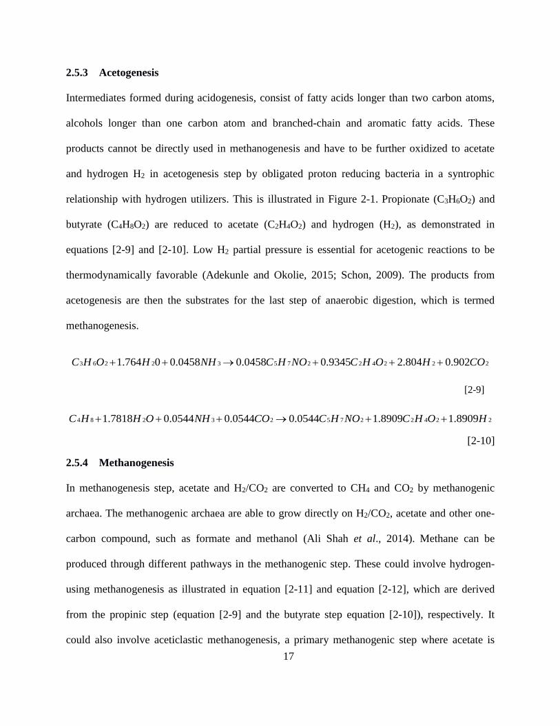
2.5.3 Acetogenesis

Intermediates formed during acidogenesis, consist of fatty acids longer than two carbon atoms,

alcohols longer than one carbon atom and branched-chain and aromatic fatty acids. These

products cannot be directly used in methanogenesis and have to be further oxidized to acetate

and hydrogen H2 in acetogenesis step by obligated proton reducing bacteria in a syntrophic

relationship with hydrogen utilizers. This is illustrated in Figure 2-1. Propionate (C3H6O2) and

butyrate (C4H8O2) are reduced to acetate (C2H4O2) and hydrogen (H2), as demonstrated in

equations [2-9] and [2-10]. Low H2 partial pressure is essential for acetogenic reactions to be

thermodynamically favorable (Adekunle and Okolie, 2015; Schon, 2009). The products from

acetogenesis are then the substrates for the last step of anaerobic digestion, which is termed

methanogenesis.

3 6 2 2 3 5 7 2 2 4 2 2 21.764 0 0.0458 0.0458 0.9345 2.804 0.902C H O H NH C H NO C H O H CO

[2-9]

4 8 2 3 2 5 7 2 2 4 2 21.7818 0.0544 0.0544 0.0544 1.8909 1.8909C H H O NH CO C H NO C H O H

[2-10]

2.5.4 Methanogenesis

In methanogenesis step, acetate and H2/CO2 are converted to CH4 and CO2 by methanogenic

archaea. The methanogenic archaea are able to grow directly on H2/CO2, acetate and other one-

carbon compound, such as formate and methanol (Ali Shah et al., 2014). Methane can be

produced through different pathways in the methanogenic step. These could involve hydrogen-

using methanogenesis as illustrated in equation [2-11] and equation [2-12], which are derived

from the propinic step (equation [2-9] and the butyrate step equation [2-10]), respectively. It

could also involve aceticlastic methanogenesis, a primary methanogenic step where acetate is

18

broken down to evolve CH4 and CO2 as illustrated in equation [2-13]. In the normal anaerobic

digesters, acetate is the precursor for up to 70% of total methane formation while the remaining

30% originates from H2/CO2 (Panico et al., 2014). Moreover, the inter-conversion between

hydrogen and acetate, catalyzed by homoacetogenic bacteria, also plays an important role in the

methane formation pathway. Homoacetogens can either oxidize or synthesize acetate depending

on the hydrogen concentration in the system (Kotsyurbenko, 2005). Hydrogenotrophic

methanogenesis functions better at high hydrogen partial pressure, while aceticlastic

methanogenesis is independent on hydrogen partial pressure. Protein and lipid conversion to

acetate involves sequential aceticlastic methanogenesis reactions as described by equation [2-13]

(Yu et al, 2013). At higher temperatures, the acetate oxidation pathway becomes more favorable

(Appels et al., 2008). Methane formation through acetate oxidation can contribute up to 14% of

total acetate conversion to methane under thermophilic conditions (60°C) (Weedermann et al.,

2015).

[2-11]

[2-12]

[2-13]

2.6 Methanogens

Methanogenic archaea are a phylogenetically diverse group of strictly anaerobic Euryarchaeota

with an energy metabolism that is restricted to the formation of methane from CO2 and H2,

formate, methanol, methylamines and/or acetate (Garcia et al., 2000). Methanogens can be

19

classified as Gram-positive or Gram-negative. They can also be motile (flagellated) or immotile

bacteria. Usually, methanogens are coccoid (spherical), spirillum or bacilli (rod) in shape.

Methanogens are classified into five orders (Figure 2-2) namely, Methanobacteriales,

Methanococcales, Methanosarcinales, Methanomicrobiales and Methanopyrales. Changes in

taxonomy and variation of the orthographic of the methanogens have contributes to different

names of the methanogens of the same species.

There has been development in the biotechnology of biogas production technology and microbial

community with recent studies on phylogenetic characterization of a biogas plant microbial

community integrating clone library 16S-rDNA sequences and metagenome sequence data

obtained by 454-pyrosequencing by Kröber et al., (2009). In his study, most of the bacterial 16S-

rDNA sequences could be assigned to the phylum Firmicutes with Clostridia as the most

abundant class and to the class Bacteroidetes, while the archaeal 16S-rDNA sequences were

clustered close to Methanoculleus bourgensis. A large fraction of 16S-rDNAmetagenome reads

could not be assigned to lower taxonomic ranks, demonstrating that numerous microorganisms in

the biogas plant are still unclassified or unknown. In addition, literature on the contribution of

each bacterial strain to the yield of biogas production is scanty, hence the knowledge gap.

A study by Sinbuathong et al., (2009) on the effect of sulfate on the methanogenic activity of a

bacterial culture was increased and reached optimum values of 0.128 g methane gas COD/(g

VSS x d) when biomass was in contact with sulfate at a ratio of 1:0.114 by weight. In a study on

the enhancing effect of aerobic thermophilic (AT) bacteria on the production of biogas from

anaerobically digested sewage sludge (Miah et al., 2005), it was concluded that addition of 5%

20

(v/v) AT1 bacterial culture closely related to Geobacillus thermodenitrificans increased biogas

production by 2.2 times relative to that from the sewage sludge.

21

Figure 2-2: Biodiversity of Methanogens

Source: Classification of methanogenic bacteria by Zuo et al., 2015

22

2.7 Factors affecting biogas production

Efficient utilization of brewery waste water offers an opportunity to produce renewable energy

and also reduce greenhouse gas (GHG) emissions. Anaerobic digestion is an essential process for

the production of biogas and the main parameters affecting methanogenic reactions in a

biodigester include but not limited to nutrient concentration, pH value and temperature among

others. These factors need to be controlled to allow maximum growth of the microorganisms

involved in the AD.

2.7.1 Nutrient concentration

Organic matters, which are broken down by microorganisms without oxygen, often produces

some quantities of methane. All biological process requires adequate nutrients supply

particularly Carbon and Nitrogen as well as other elements are also required in trace quantities.

The lack of specific elements required for microorganism growth will limit the production of

biogas (Sorathia et al., 2012). Carbohydrates supplies Carbon which is a source of energy, while the

proteins provide Nitrogen needed for the growth of microbial organisms. If the other operating conditions

are made favourable for the production of biogas and maximum biological activity, a Carbon to Nitrogen

ration of about 30:1 is reported to be ultimate for the raw materials with 2% Phosphorous fed into a

biodigestor. A higher carbon to nitrogen ratio will result in excess carbon still available after complete

consumption of the nitrogen starving some of the bacteria of this element, leading to the death and

returning nitrogen to the mixture, with the net effect of slowing the process. Excess of nitrogen at the end

of digestion, which stops when the carbon has been consumed, and reduce the quality of the sludge

produced. Thus, nutrients like C, P and N2 are to be maintained within the optimum range for accelerated

fermentation and biogas production (Fillaudeau et al., 2006; Macias-Corral et al., 2008).

23

2.7.2 pH

Hydrocarbons are easier to acidify and no pH-buffering ions are released as with the

degradation of proteins. Therefore, the pH-value decreases more easily. With the degradation

of carbohydrates, the partial pressure of hydrogen increases more easily, as with other

substances. This happens in combination with the formation of reduced acidic intermediate

products. The pH optimum of the methane-forming microorganism is at pH of 6.8-7.2.

Therefore, it is important to adjust the pH-value. Only Methanosarcina is able to withstand

lower pH values (pH of 6.5 and below). With the other bacteria, the metabolism is

considerably suppressed at pH <6.7 (Jayaraj et al., 2014).

2.7.3 Temperature

For maximum gas yield, different temperature ranges exist for which the mesophilic and

thermophilic bacteria are most active. Two optimum temperature levels have been established

the mesophilic level (35-40°C) and thermophilic level (50-65°C) (Jha et al., 2011), the choice

of which is determined by the natural climatic conditions where the biodigestor is located.

Most of the methanogenic microorganisms belong to the mesophilics. Only a few are

thermophilic. Methanogenics are generally sensitive to rapid changes of temperature.

Thermophilic methanogens are more temperature-sensitive than mesophilics. Even small

variations in temperature cause a substantial decrease in activity. Therefore, the temperature

should be kept exactly within a range of +/- 2°C. Under mesophilic operating conditions, the

inhibition of ammonium is reduced because of the lower content of inhibiting free ammonia.

It has to be established that the energy balance is better in the mesophilic range than in the

thermophilic range (Cioabla et al., 2012).

24

2.8 Isolation and characterization of bacteria

A wide range of media has been used to estimate the size of the bacterial community of waste

water treatment systems and to isolate representatives of these communities (Vieira and Nahas,

2005) although, only a small part of the total number of bacteria in the sample, are able to form

colonies on microbiological media (Davis et al., 2005).

There are many practical applications for identifying unknown bacteria. Primary identification

involves morphological and biochemical characterization among others. Morphological

characterization involves identification of bacteria using visible characteristics of the colony

e.g colour, although it’s not a reliable way to identify bacteria, as many different types of

bacteria have similar colony morphology. Biochemical characterization however is based on

the reaction of different microorganisms to biochemical test since each microorganism has a

unique DNA that is able to synthesize different protein enzymes that catalyze all of the various

chemical reactions. This, in turn, means that different species of bacteria must carry out

different and unique sets of biochemical reactions. Molecular techniques are equally important

in the analysis of microorganisms as they are effective and fast technology for identification of

microbial diversity in different environments (Clarridge, 2004). Genetic diversity can identify

individual organisms from some unique part of their DNA or RNA providing definitive

information on its biodiversity. In molecular techniques, bacteria are generally identified by

16S ribosomal DNA (rDNA) sequencing. It is a well-established method for studying

phylogeny and taxonomy of samples from various environments. 16S rDNA is the most

conserved gene in all cells and portions of this rDNA sequence from distantly-related

organisms are remarkably similar, indicating that, sequences from distantly related organisms

can be precisely aligned, hence ease in estimating rates of species divergence among bacteria

25

(Janda and Abbott, 2007). The 16S rDNA sequence has hyper variable regions, where

sequences have diverged over evolutionary time which are often flanked by strongly-conserved

regions. Primers are designed to bind to conserved regions and amplify variable regions. The

DNA sequence of the16S rDNA gene has been determined for an extremely large number of

species. Sequences from tens of thousands of clinical and environmental isolates are available

over the internet through the NCBI (National Centre for Biotechnology Information)

(www.ncbi.nlm.nih.gov). These sites also provide search algorithms to compare new sequences

to their database.

2.9 Modelling microbial growth

2.9.1 Microbial growth

A growing population of bacteria periodically doubles when grown in the laboratory under

favorable conditions. They grow in geometric progression of 20, 21, 22, 23 ......... 2n, where n is

the number of generations during the exponential phase. Exponential phase in reality only

forms part of the bacterial life cycle but does not represent the pattern of the normal growth of

bacteria in nature (Prescott, 2002).

When a fresh medium is inoculated with a given number of cells and the population growth is

monitored over a period of time. The growth curve is commonly expressed in terms of

microbial numbers, but can also be expressed in terms of optical density as an indirect

measurement. Optical density method uses absorbance measurement which is a rapid,

nondestructive, inexpensive, and relatively automated method to monitor bacterial growth, as

compared to many other techniques like classical viable count methods (Pla et al., 2015).

Plotting the population growth verses time data yields a typical bacterial growth curve which is

26

usually divided into the lag phase, exponential phase and the stationary phase as illustrated in

Figure 2-3 (Joanne et al., 2016).

Lag Phase.

In this phase, the population remains temporarily unchanged immediately after inoculation of

the cells into fresh medium. Although there is no apparent cell division occurring, the cells may

grow in volume or mass, synthesizing enzymes, proteins, RNA and increase in metabolic

activity. The length of the lag phase depends on various factors, including, without limitation

on the size of the inoculum, the time from physical damage or shock required to recover in the

transmission, time required for synthesis of essential coenzymes or division factors, and time

required for synthesis of new enzymes that are necessary to metabolize the substrates present in

the medium. The growth is approximately equal to zero, thus;

[2-14]

Exponential (log) phase.

The cells divide regularly by binary fission, and grow by geometric progression. They divide at

a constant rate depending upon the composition of the growth medium and the conditions of

incubation. The rate of exponential growth of a bacterial culture is expressed as generation time,

also known as the doubling time of the bacterial population. The growth can be represented as;

Where n represents the number of doublings occurred after some time interval.

Thus,

27

. [2-15]

Where; td is the doubling time in hours. It follows therefore that the number of cells present at

time t, in relation to the initial population is given as;

[2-16]

Where, n= represents the number of generation,

N=Final number of cells

N0=Initial number of cells

Substituting the value of n in equation [2-16] gives;

[2-17]

Similarly,

[2-18]

Taking logarithms,

Which is the same as,

[2-19]

Plotting the natural logarithm of the number of cells against time of incubation should yield as

28

straight line whose slope is equivalent to . Thus,

[2-20]

The specific growth rate constant (the rate of increase in the number of cells per unit time can be

given by;

, [2-21]

Where;

is the specific growth rate usually symbolically written as µ and the units are in

reciprocal hours (h-1).

Stationary phase.

Exponential growth cannot be continued forever in a batch culture (e.g. a closed system such as

a test tube or flask). Population growth is limited by a number of factors including but not

limited to exhaustion of available nutrients; accumulation of inhibitory metabolites or end

products; and exhaustion of space. During the stationary phase, if viable cells are being counted,

it cannot be determined whether some cells are dying and an equal number of cells are dividing,

or the population of cells has simply stopped growing and dividing. The stationary phase, like

the lag phase, is not necessarily a period of quiescence. Bacteria that produce secondary

metabolites, such as antibiotics, do so during the stationary phase of the growth cycle. It is

during the stationary phase that spore-forming bacteria have to induce or unmask the activity of

29

dozens of genes that may be involved in sporulation process.

Death phase.

If incubation continues after the population reaches stationary phase, a death phase follows, in

which the viable cell population declines. The death phase cannot be observed if counting is

done by turbidimetric measurements or microscopic counts. During the death phase, the number

of viable cells decreases geometrically (exponentially), essentially the reverse of growth during

the log phase.

Figure 2-3: Microbial growth curve

Source: Modified from Joanne et al., 2016

30

2.9.2 Microbial growth models

Microbial models are mathematical expressions that describe the number of microorganisms in a

given system, as a function of relevant intrinsic or extrinsic variables, generally on a

macroscopic scale. Modeling is an important tool for understanding microbial growth in the

processes such as safe food production, wastewater treatment, bioremediation, or microbe-

mediated and mining among others (Esser et a.l, 2015; Marks, 2008; Mitchell et al., 2004) and

could also be used as virtual laboratories to optimize experimental design (Pla et al, 2015). They

can be classified as primary, secondary or tertiary. Primary models describe how the number of

microorganisms in a population changes with time under specific conditions. Secondary models

relate the primary model parameters to environmental or intrinsic variables such as temperature

or pH. Tertiary models combine primary and secondary models with a computer interface

providing a complete prediction tool (Marks, 2008).

For the models to be constructed, growth has to be monitored and modelled. Several primary

growth models exist in the literature, such as the models by Gompertz, Richards, Stannard et al.,

Schnute, and the logistic model among others (Longhi et al., 2013; Zwietering et al.,1990). Table

2-2 shows their mathematical and modified forms, which gives biological meaning to the

parameters.

This mathematical equations and their modified biological form differ in “ease of use” and

number of parameters in the equation (DaSilva et al., 2012). Model selection seems to be biased

though, Gompertz, Richards, and logistic, are the most commonly used (Pla et al., 2015).

31

Table 2-2: Sigmoidal microbial growth models and their biological modified forms

MODEL MATHEMATICAL EQUATION MODIFIED EQUATION

Logistic

[1 exp( )]

ay

b cx

max4{1 exp[ ( ) 2]}

oA

y y

tA

Gompertz exp[ exp( )]y a b cx max .exp{ exp[ ( ) 1]}o

ey y A t

A

Richards

1( ){1 .exp[ ( )}y a k x

max 1 1{1 .exp(1 ).exp[ .(1 )(1 ).( )]}( )oy y A t

A

Stannard ( )

(1 ){1 exp[ ]} p

kxy a

p

max 1 1{1 .exp(1 ).exp[ .(1 )(1 ).( )]}( )oy y A t

A

Schnute 1

2 1

1 exp[ ( )] 1{ ( ). }

1 2 1 1 exp[ ( )]

b b b a ty y y

a b

y

(1 ) 1 .exp( . 1 ) 1( max )[ ]

1o

b b a b aty y

a b b

Source; Zwietering, 1990

Legend; a a, b, c are mathematical parameters, A is the asymptote of growth curve when population reaches maximum, μmax is the maximum of specific growth

rate, λ is the lag time

32

The models have different number of growth parameters defined by the growth curve thus there

may be existence of difference in the results obtained using different growth models (Zwietering

et al.,1990). The growth of bacterial usually goes through a phase in which the specific growth

rate (the tangent in the inflection point) starts at a value of zero and then accelerates to a maximal

value (µmax) in a certain period of time, resulting in a lag time (λ), (the x-axis intercept of the

tangent in the inflection point). The asymptote is the maximal log10 N value reached illustrated

as the point at which there is maximum population in Figure 2-3, resulting in sigmoidal curves.

The models with four parameters also contain a shape parameter (v).

The behaviour of different growth models have been compared in literature ranging from

different mathematical measures of goodness of fit and/or other statistical criteria (Pla et al.,

2015; Tsoularis and Wallace, 2002). Direct comparisons of specific growth parameters as

predicted by various models have also been explored with different conclusions, hence, there is

substantial disparity in literature on which is the best-fitting model for predicting microbial

growth (Longhi et al., 2013; Perni et al., 2005).The modified stannard equation appears to be the

same as the modified Richards equation (Table 2-2),with four growth parameters (A, µmax, λ and

ν).The ν, in the four parameter models represents the shape parameter which is difficult to

explain biologically, and are significantly better to use when a large number of datum points are

collected (Zwietering et al., 1990). However, three parameter models have more degrees of

freedom for the parameter estimates which can very useful when growth curves of small number

of measured points is used.

33

2.10 Overview of methodology adopted for the study

The accurate and definitive identification of microorganisms, including bacteria, is important

wastewater treatment, food safety, bioremediation, mining among others. Identification is based

upon the labelling of bacteria, parasites, and fungi with appropriate binomial names of Latin or

Greek origin (Janda and Abbott, 2002). Various techniques for bacteria identification exist

ranging from the rapid analysis to the use of molecular methods to provide genus and species

identification (Petti, 2007). Bacterial can be identification can using genotypic techniques based

on profiling an organism’s genetic material (primarily its DNA) and phenotypic techniques based

on profiling either an organism’s metabolic attributes or some aspect of its chemical

composition. Genotypic techniques have the advantage of being independent of the physiological

state of an organism unlike the phenotypic methods. Phenotypic techniques, however, can yield

more direct functional information that reveals what metabolic activities are taking place to aid

the survival, growth, and development of the organism (Emerson et al., 2008).

Genotypic microbial identification methods can be classified into two broad categories including

the pattern or fingerprint-based techniques and sequence-based techniques. Pattern-based

techniques typically use a systematic method to produce a series of fragments from an

organism’s chromosomal DNA. These fragments are then separated by size to generate a pro-

file, or fingerprint that is unique to that organism and its very close relatives. With enough of this

information, researchers can create a library, or database, of fingerprints from known organisms,

to which test organisms can be compared. When the profiles of two organisms match, they can

be considered very closely related, usually at the strain or species level. Sequence-based

techniques rely on determining the sequence of a specific stretch of DNA, usually, but not

always, associated with a specific gene (Mcdonald et al., 2012; Stackebrandt et al., 2012). The

34

degree of similarity, or match, between the two sequences is a measurement of how closely

related the two organisms are to one another. A number of computer algorithms have been

created that can compare multiple sequences to one another and build a phylogenetic tree based

on the results. Sequence-based techniques have proved effective in establishing broader

phylogenetic relationships among bacteria at the genus, family, order, and phylum levels,

whereas fingerprinting-based methods are good at distinguishing strain or species level

relationships but are less reliable for establishing relatedness above the species or genus level

(Emerson et al., 2008).

2.11 Summary of literature review

As the utmost common process for the biological treatment of wastewater and biogas production,

AD has gained significant importance, albeit problems such as low methane yield and process

instability, preventing this technique from being widely applied. This process requires

synergistic efforts of various microorganisms in various steps as discussed, where the products of

one step are utilized in the next one finally culminating in the production of biogas. Acid

forming and the methane forming microorganisms vary broadly in terms of structure, nutritional

needs, growth kinetics, and sensitivity to environmental conditions. Thus, failure to maintain the

balance between these two groups of microorganisms is the primary cause of reactor instability.

Among the important methanogenis processes within AD are the hydrogenotrophic

methanogenesis and aceticlastic methanogenesis, which, when they are inhibited, the digestion is

effectively blocked at acidogenesis. In addition, the low growth rates and the susceptibility of the

organisms to toxins increases the difficulties in the optimization of methanogenesis.

35

Methanogenic reactions are usually affected by various factors including microbial growth,

nutrient concentration, pH value and temperature among others. These factors need to be

controlled to allow maximum growth of the microorganisms involved in the AD. The growth of

microorganisms can be monitored over a period of time when a given number of cells have been

inoculated in afresh medium, and these growths have been modelled for different operations

using both primary and secondary models.

Investigation of methanogens can assist in not only the classification but also the optimization of

the AD systems. Thus, the study builds on the analysis of the biodegradability index of the

brewery waste water and primary microbial growth models developed by Gomperzt and Logistic

to describe the growth of the methanogenic community in a bio-digester as a function of time. In

industrial applications of anaerobic digestion for biogas generation, the focus is to stabilize and

capitalize on biogas production.

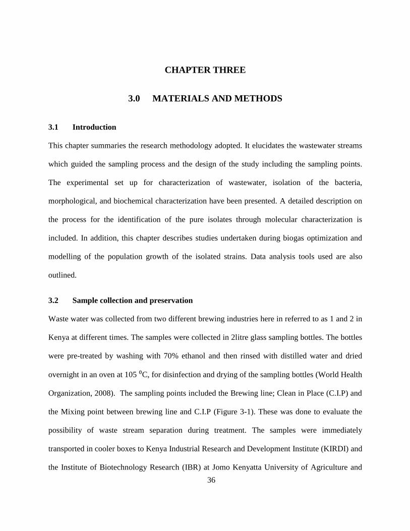
36

CHAPTER THREE

3.0 MATERIALS AND METHODS

3.1 Introduction

This chapter summaries the research methodology adopted. It elucidates the wastewater streams

which guided the sampling process and the design of the study including the sampling points.

The experimental set up for characterization of wastewater, isolation of the bacteria,

morphological, and biochemical characterization have been presented. A detailed description on

the process for the identification of the pure isolates through molecular characterization is

included. In addition, this chapter describes studies undertaken during biogas optimization and

modelling of the population growth of the isolated strains. Data analysis tools used are also

outlined.

3.2 Sample collection and preservation

Waste water was collected from two different brewing industries here in referred to as 1 and 2 in

Kenya at different times. The samples were collected in 2litre glass sampling bottles. The bottles

were pre-treated by washing with 70% ethanol and then rinsed with distilled water and dried

overnight in an oven at 105 ⁰C, for disinfection and drying of the sampling bottles (World Health

Organization, 2008). The sampling points included the Brewing line; Clean in Place (C.I.P) and

the Mixing point between brewing line and C.I.P (Figure 3-1). These was done to evaluate the

possibility of waste stream separation during treatment. The samples were immediately

transported in cooler boxes to Kenya Industrial Research and Development Institute (KIRDI) and

the Institute of Biotechnology Research (IBR) at Jomo Kenyatta University of Agriculture and

37

Technology (JKUAT) laboratories and stored at 4⁰C without further treatment, until they were

analyzed.

Rinsing and cleaning of

equipment

Flushing of filter

Keg washing

- Cleaning of packaging

material, floors

- Soap lubrication of

conveyors in packaging

area

Cooling water

CIP lineBrewing line

Mixing point

To WWTP

Sampling point

Figure 3-1: Sampling points

3.3 Characterization of Brewery waste water and evaluation of its potential for Biogas

Production

Analyses of the samples were all carried out at KIRDI Laboratories. The samples were analyzed

as per Standard Method for the examination of water and wastewater (APHA, 2005). The

physicochemical characteristics measured include: BOD5, COD, TDS, TSS, TS, sodium, Total

nitrogen and Total phosphorous.

3.3.1 Laboratory analysis

Total solids, Total dissolved solids (TDS), Total suspended solids

Total solids were determined by gravimetric method and then suspended solids were calculated

by using equation [3-1].

38

[3-1]

Biochemical Oxygen Demand (BOD)

BOD was estimated by preparing required volume of dilution water with the addition of nutrients

namely phosphate buffer, magnesium sulfate, calcium chloride and ferric chloride. The diluted

sample was transferred to BOD bottles. After determining initial DO, final DO was estimated of

the bottles kept for incubation period of five days. The bottles kept for DO determination and

blank were fixed by adding 2ml manganese sulfate (MnSO4), 2ml of alkali iodide azide

( ).

Chemical Oxygen Demand (COD)

COD determination was carried out with dichromate reflux method with the addition of 10 ml of

0.25 N potassium dichromate (K2Cr2O7) and 30 ml reagent in 20 ml

diluted sample. The mixture was refluxed for 2 hours and was cooled to room temperature. The

solution was then diluted to 150ml by using distilled water and excess K2Cr2O7 remained was

titrated with ferrous ammonium sulfate (FAS) using ferroin indicator. The COD values were

determined using equation [3-2]

[3-2]

Where A is the ml of FAS used for blank; B is the ml of FAS used for sample, N is the normality

of FAS and 8 is milli equivalent weight of oxygen

39

Total Nitrogen

The Nitrogen levels were determined using Kjeldahl method, developed by Johan Kjeldahl,

where the sample was weighed, digested, neutralized and the nitrogen estimated by titration.

Sodium

The sodium levels were determined using Atomic Absorption Spectrophotometer equipment

(AAS). Prior to measurement, the sample were digested in 1:1HCL on a sand bath. After

digestion, distilled water was used to take to mark and the sample subjected to AAS.

Phosphorous

The phosphorus levels were determined using UV spectrophotometer. Prior to measurement, the

samples were digested in 1:1 HCL on a sand bath. After digestion, distilled water was used to

take to mark and a complexing reagent (molybdate) added and color change observed. The

sample was then read on the instrument.

3.4 Isolation and Characterization of Methanogenic bacteria from brewery wastewater

To evaluate the microbial population of the brewery wastewater, methane producing bacteria

were isolated as a step towards optimization of biogas production. Both morphological and

molecular techniques were used during the identification of the isolates. Samples from Brewing

Industry 1 were used as inoculum.

3.4.1 Isolation of wastewater bacteria

Brewer thyglycollate media from Oxoid was used for cultivation of the anaerobic bacteria. It

consisted of 1.0 g lab-Lemco’ powder, 2.0 g yeast extract, 5.0 g peptone, 5.0 g glucose, 5.0 g

sodium chloride, 1.1 g sodium thioglycollate, 0.002 g methylene blue and 1.0 agar at pH 7.2 ±

40

0.2 per litre. Twenty grams of the medium was suspended in 1 litre of distilled water, brought to

boil, mixed well and allowed to stand until completely dissolved. 40 ml were dispersed into 100

ml screw cap glass test tubes and sterilised by autoclaving at 121°C for 15 minutes. One

millilitre of each sample was inoculated at the base of each test tube using a sterile syringe and

incubated at 37⁰C in an anaerobic jar. Observations for growth were made after every 12 hours.

Serial dilutions of 12 hours old bacteria culture in the ratios of 100, 10-1, 10-2, 10-3, 10-4, and 10-5

were transferred to petri-dishes containing brewer thyglycollate media with modification and

spread over the surface with a sterile glass spreading rod. Each dilution series was used to

inoculate a series of plates with two plates at each dilution level and incubated in an anaerobic

jar (Plate 3-1). Anaerobic jar was evacuated by placing a kindled candle, which quenches

immediately the left over oxygen. The jar was incubated for a period of 72 hours at 37°C. The

colonies that emerged on the plates were sub-cultured repeatedly on fresh plates to obtain pure

isolates.

3.4.2 Morphological characterization.

Preliminary characterization of the isolates involved the examination of colony morphology,

(Plate3-2 (1a-1d)). Culture features such as colour, pigmentation, elevation, shape, size and

growth form, of safranin-stained bacterial isolates were observed under the dissecting and

compound microscope using the slide procedure (Holt et al., 1994).

3.4.2.1 Gram staining of the isolated bacteria

Smears of bacteria cultures were prepared and heat-fixed. Slides were placed on the staining rack

and flooded with crystal violet and allowed to stand for 30 seconds. The slides were then rinsed

with water for 5 seconds followed by covering with Gram’s iodine mordant. They were then

41

allowed to stand for 1 minute and rinsed with water for 5 seconds. Decolonization was done with

95% ethanol for 15 to 30 seconds followed by rinsing with water for 5 seconds. Counterstaining

was done using Safranin for about 60 to 80 seconds and the slides were rinsed again with water

for 5 seconds.

Blot drying was carried out using a bibulous paper and examined using microscope at x100

under oil immersion (Srinivasan et al., 2012). Gram-positive organisms stained blue to purple;

Gram-negative organisms stained pink to red. Gram staining results were confirmed by using the

3% KOH test (Chandra and Mani, 2011). This test was performed by adding a drop of 3% KOH

on a slide. A loop full of the bacteria was introduced and mixed thoroughly. Positive results were

observed if the culture pulled along with the wire loop when raised up and negative results were

recorded if nothing was pulled along the wire loop.

42

Plate 3-1: (1a) Autoclaved media on plates and tubes for inoculation. (1b) incubation in

anaerobic jar. (1c) Growth on plates. (1d) Pure strains sub-cultured in

Eppendorf tubes

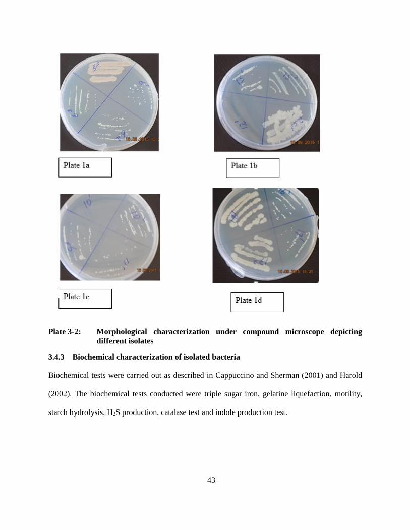
43

Plate 3-2: Morphological characterization under compound microscope depicting

different isolates

3.4.3 Biochemical characterization of isolated bacteria

Biochemical tests were carried out as described in Cappuccino and Sherman (2001) and Harold

(2002). The biochemical tests conducted were triple sugar iron, gelatine liquefaction, motility,

starch hydrolysis, H2S production, catalase test and indole production test.

44

3.4.3.1 Triple Sugar Iron Agar Test

Triple Sugar Iron contains three carbohydrates namely, glucose, sucrose and lactose. The media

also contains beef extract, yeast extract and peptones which are sources of Nitrogen, vitamins

and minerals. Agar and phenol red are also used to solidify the medium and pH indicator

respectively. The tubes containing molten agar were angled during preparation and using aseptic

technique, the TSI slant was inoculated by first stabbing the butt down to the bottom and then

streaking the surface of the slant with appropriate bacterium. The caps on the tubes were tightly

screwed not to permit access of air. Incubation was done anaerobically for 18 to 24 hours at 35°C

for changes in the butt and on the slant.

A change in the original colour of the medium (reddish-orange) to yellow indicates fermentation

of any of the carbohydrates, a red colour in both slant and butt indicates neither glucose, lactose

nor sucrose has been fermented. Presence of bubbles in the butt indicates the ability of the

bacteria to produce gas. Hydrogen sulfide production from thiosulfate is indicated by a

blackening of the butt as a result of the reaction of hydrogen sulfide with ferrous ammonium

sulfate to form a black ferrous sulfide.

3.4.3.2 Catalase test

Catalase test detects the activity of enzyme catalase that is present in most cytochrome-

containing aerobic bacteria. These microbes produce hydrogen peroxide during the aerobic

breakdown of sugars. The test was performed to determine the ability of the isolates to produce

catalase enzyme which microorganisms living in oxygenated environment use to neutralise

toxic forms of oxygen metabolites (hydrogen peroxide). Catalase enzyme neutralises the

bactericidal effects of hydrogen peroxide and thus protecting them. This enzyme catalyses the

45

breakdown of hydrogen peroxide into water et al and oxygen. Therefore, Catalase-negative

bacteria may be anaerobes, or they may be facultative anaerobes that only ferment and do not

respire using oxygen as a terminal electron acceptor (Manimegalai., 2014). Catalase test was

carried out by scooping a colony of a 24-hour culture, placing it on a glass slide and adding a

drop of 3% hydrogen peroxide solution. A positive reaction was indicated by the formation of

bubbles, while the absence of air bubbles indicated a negative catalase test.

3.4.3.3 Gelatine liquefaction/hydrolysis

Gelatine liquefaction detects the breakdown of gelatine to polypeptides and amino acids by

enzyme gelatinase. Gelatine protein is produced by hydrolysis of a component of the

connective tissues and tendons of animals known as collagen. Gelatine is solid at room

temperature but above 25oC it turns into liquid. When gelatinase hydrolyses this protein into

amino acids, it remains liquefied even at the low temperatures of an ice bath. The bacterial

isolates were inoculated onto nutrient broth supplemented with 12% gelatine and 1.5% agar, to

demonstrate hydrolytic activity of gelatinase. One uninnoculated tube was used as control for

each isolate. After incubation, cultures that remained liquefied totally or partially when placed

in refrigerator at 4 o C for 30 minutes were considered positive for gelatine hydrolysis.

3.4.3.4 Indole, Motility and Hydrogen sulphide production tests

The test identifies isolates with the ability to produce the enzymes tryptophanase that removes

the amino group from tryptophan to form Indole, pyruvic acid and ammonia, and cysteine

desulfurase, that produces pyruvate, ammonia and hydrogen sulphide from sulphur containing

amino acids. Indole reacts with Kovacs reagent (p-dimethylamino-benzaldehyde) to form a

46

deep red colour while the Iron in the medium reacts with hydrogen sulphide to produce a black

precipitate.

The isolates were inoculated in Sulphur-Indole Motility (SIM) agar media by stabbing method

in duplicate for replication, and then incubated at 37 oC for 48 hours. Two uninnoculated tubes

were used as controls. Kovac’s reagent was the added to each of the 48-hour culture. The

presence of a cherry red layer in the media indicated positive result for Indole production while

negative results were indicated by colour remaining brown. The presence of a black coloration

in the media after incubation indicated lack of hydrogen sulphide in the media. Lack of motility

was detected by the confinement of the bacteria along the line of inoculation.

3.4.3.5 Starch Hydrolysis

Using the wax pencil, starch agar plate was divided into two straight sections. Labelling was

done each with the bacterium to be inoculated. Using aseptic technique streaking was done

with the respective bacteria onto the plate in a straight line within the section. Incubation of the

plate for 24 to 48 hours at 37 o C was done. Drops of Gram’s iodine were placed on each of the

line streaked on the starch agar plate. If the area around the line of growth was clear, starch had

been hydrolysed, and the test was positive; if it was not clear or the entire medium turned blue,

starch has not been hydrolysed, and the test was negative.

3.4.4 Identification of methanogenic bacteria

Colonies of methanogenic bacteria were identified on Petri plates using Fluorescent test in which

a blue-green fluorescence, characteristic to this metabolic group of bacteria (Dhadse et al., 2012)

was observed and was distinct from the white-yellow fluorescence normally observed with non-

methanogenic bacteria. Pure isolates were subcultured on the plates and incubated anaerobically

47

in anaerobic jar at 37o C for three days. The cultures were then subjected to excitation by long

wave ultraviolet light at 312nm using Uvidoc BTS-20.M. The cultures that exhibited a bluish

green fluorescence were considered positive. To confirm this group, the isolates were sub-

cultured in brewer thyglycollate broth media and incubated anaerobically in batch digesters for 7

days in an mrc laboratory equipment water bath Bo-200. The gas produced was analysed using

Biogas 5000 analyser, with CH4 and CO2 accuracy of ±0.5% of measurement reading after

calibration.

3.4.5 Molecular characterization

Molecular characterization was used to confirm the identity of the isolates. Total bacterial DNA

was extracted according to the procedures described by Sambrook et al. (1982) and Magarvey et

al., (2004). Bacterial 16S rDNA genes of the pure isolates were amplified and used as a template

for amplification of 16S rDNA gene.

3.4.5.1 DNA Extraction

Genomic DNA was extracted from bacteria cells at exponential growth phase grown

anaerobically in Brewer Thyglycollate broth media. Prior to extraction, bacterial cells were

harvested from broth by centrifuging 1 ml of culture in a 1.5 ml Eppendorf tube at 13,000 rpm

for 10 minutes. The pellet was washed by re-suspending the cells in equal volume of TE buffer,

centrifuged for 5 minutes at 13,000 rpm and the supernatant discarded. The cells were re-

suspended in 200 µl of solution 1(A) [50 mM Tris pH 8, 50 mM EDTA pH 8 and 25% sucrose

solution), 20µl of lysozyme (20 mg/ml) and 10µl of RNase A (20 mg/ml) then mixed gently. The

mixture was then incubated at 37 oC for 1 hour. After 1hr, 600 µl of solution 2 (B) (10 mM Tris

pH 8, 5mM EDTA pH 8 and 1% sodium dodecyl sulphate] and 10 µl of proteinase K (20 mg/ml)

48

were added and mixed gently (appendix 2). The solution was incubated at 55 oC for 1 hr. The

DNA was extracted using equal volume of phenol chloroform (1:1) and mixed by inversion for 5

minutes, followed by centrifuging for 10 minutes at 10000 rpm. The aqueous layer was carefully

transferred into a 1.5 ml Eppendorf tube. This step was repeated twice before adding 500 µl of

chloroform: Isoamylalcohol (24:1). This step was to wash off the excess phenol.

The mixture was then mixed by inversion for 5 minutes followed by centrifuging at 10000 rpm

for 10 minutes and the supernatant carefully transferred into a clean Eppendorf tube. This step

was repeated twice. The DNA was precipitated by adding an equal volume of ice cold absolute

ethanol and 1/10 µl of sodium chloride and incubated overnight at -20o C. It was then centrifuged

at 13,000 rpm for 10 minutes and the supernatant discarded. 500 µl of 70% ethanol was added

and centrifuged at 13,000 rpm for 10 minutes. The supernatant was discarded carefully. The

pellets were then air-dried at room temperature and re-suspended in 100 µl of TE buffer and kept

at ̵ 20oC for future use. The DNA was visualised on a 1% agarose gel in 1XTBE buffer under

UV after staining with ethidium bromide.

3.4.5.2 DNA amplification

PCR amplification was performed using PeQlab advanced Primus 96 Hamburg thermal cycler

(Applied Biosystems), using universal primers pair combination of forward primer 8F forward

5’-AG (A/G) GTTTGATCCTGGCT-3’) and 1492R reverse, 5’-GGCTACCTTGTTACGACTT-

3’ according to the position in relation to Escherichia coli gene sequence (Bergmann et al.,

2010). DNA was amplified in a 50 µl mixture containing 0.30 µl of gene script Taq, 2.5 µl (10

pmol/ µl) of 8F forward primer, 2.5 µl (10 pmol/µl) of 1492R reverse primer, 10 µl of template

DNA (10 ng/µl), and 6.0 µl of dNTP’s mix (1.25 mM), 5.0 µl PCR 10 X buffer with mgcl2 and

49

23.7 µl of PCR water. Reaction mixtures were subjected to the following temperature cycling

profiles repeated for 32 cycles: Initial denaturation at 94°C for 5 min, denaturation at 94 °C for 1

min, primer annealing at 49 °C for 1 min, extension at 72 °C for 2 min and a final extension at 72

°C for 10 min (Roux, 1995). Agarose gel 1%, stained with ethidium bromide was used to

confirm amplified PCR products.

3.4.5.3 Restriction analysis of the PCR products

The preliminary genetic diversity was determined by amplified ribosomal DNA restriction

analysis (ARDRA) of 16S rDNA using a modified procedure (Desaint et al, 2000). Aliquot of 8

µl of the PCR product was digested in a final volume of 30µl for 12 hours at 37o C with 0.5 µl of

a restriction endonuclease (RsaI) according to the manufacturer’s specifications (Sigma Aldrich,

Steinheim, Germany). Digested DNA fragments were separated by electrophoresis in 1.5 (w/v)

agarose gels (Sigma Aldrich, Steinheim, Germany) for 2 hours at 80 V. The gel was stained with

ethidium bromide and DNA fragments visualised under UV illumination (BTS-20.M, EEC,

Taiwan). Similarity among strains was estimated from the proposition of shared restriction

fragments bands generated by RsaI digestion.

3.4.5.4 Agarose gel electrophoresis

Preparation of Agarose gel (w/v) at 1% was done by dissolving 1.0 g of agarose powder into100

ml of 1XTBE buffer. The gel solution was stirred, brought to boil in a microwave for 3 minutes

to completely dissolve the powder, the cooled gel solution was poured in a casting tray having

combs and left for sometimes to gel (polymerise). Ethidium bromide (3 µl) was incorporated in

the gel to facilitate visualisation of DNA under UV light. The PCR products (7 µl) was mixed

50

with 3 µl of loading dye (Bromophenol blue) and loaded into the well and subjected to

electrophoresis at 80 V for 45 minutes.

3.4.5.5 Purification of PCR products

The PCR products were purified using the QIAquick PCR purification Kit protocol (Qiagen,

Germany) according to manufacturer’s instructions. Five volumes of buffer PB (binding buffer)

(Qiagen, Germany) was added to one volume of the PCR sample and thoroughly mixed. The

mixture was then transferred to QIAquick spin column and then centrifuged for three minutes at

8000 g. The flow-through was discarded, and the QIAquick column placed back into the same

tubes. To wash the DNA, 740µl buffer PE (washing buffer) was added to the QIAquick column

twice and centrifuged for one minute. The flow-through was discarded and the column

centrifuged again for an additional one minute at 8000 g to remove residual ethanol from buffer

PE. The QIAquick column was placed in a 1.5 ml microcentrifuge and 30 l of buffer EB

(elution buffer) (10 mM Tris-Chloride, pH 8.5) added to elute DNA. The tubes were then

centrifuged for one minute, the spin column removed and DNA. The tubes were then centrifuged

for one minute at 8000 g, the spin column removed and DNA stored at ̵20o C.

3.5 Optimization of biogas from isolated strains

Optimization of the environmental conditions involved variations in temperature and pH. In

addition, modified biological equations from mathematical models were used to predict the

growth of the isolated methanogenic stains at a constant temperature of 37°C.

3.5.1 Effect of temperature and pH on methane production

Anaerobic digestion experiments to measure the methane produced were carried out using

Brewer Thyglycollate media (appendix 1), 250 ml vacuum flasks were used as batch digesters

51

and the temperatures studied included 30 ºC, 35 ºC, 37 ºC and 40 ºC, with a pH range of 6.0,7.2

and 8. The methane yields from each experimental setup, Plate 3-3, were measured with Biogas

5000 gas analyzer with CH4 and CO2 accuracy of ±0.5%of measurement reading after

calibration. Each experimental set up were done and recorded in triplicates. Both methane yield

and biogas quality (CH4, CO2, O2 and H2S,) were investigated and were recorded at the end of

the incubation period of seven days. The cumulative volume of the gas produced during the

incubation period was estimated by measuring the initial and final pressure in the 250 ml vacuum

flasks and applying the ideal gas law to calculate the volume as illustrated in equation [3-4]. The

Initial pressure was indicated on the KIF LAB Labotporp vacuum pump during air evacuation

and the final pressure was as indicated by barometer on the biogas analyzer 5000.

2 1( ) r agas

a r

P P V TV

P T

[3-4]

Where;

V gas = volume of cumulated gas produced (mL);

P1 = Initial pressure of the as indicated by the vacuum pump (kPa);

P2 = Final pressure after incubation period (kPa);

Pa = ambient pressure

Ta = ambient (Initial) temperature (K);

Tr = temperature of the reactor (vacuum flask) (K);

Vr = capacity of the vacuum flask (250mL).

52

Methane production (ml) =Total gas produced (ml) × percentage methane in the sample

Plate 3-3: Experimental set up for biogas analysis in the bio-digester

3.5.2 Calibration of the equipment

The BIOGAS 5000 gas analyzer was calibrated once every week, the Zero’ and ‘Span’. Zero

experiments. The Zero experiment was the point at which the gas analyzer was calibrated when

there was none of the methane gas present (in the open field). Span Zero was at the point at

which the gas analyser was calibrated when a known quantity of the methane gas was present

using cooking gas from Total Kenya. Zeroing of the gas analyser was undertaken at the start of

each week’s monitoring.

3.5.3 Monitoring growth rate of the isolates at 37°C

Growth can be defined as an increase in cellular constituents and may result in an increase in a

microorganism’s size, population number, or both (Prescott, 2002). Freshly cultured 12 hour old

53

cells of pure isolates were used in this experiment. 200µl of the cells were inoculated in a closed

culture vessel of 800µl brewer Thyglycollate single batch media after autoclaving at 121ºC. The

contents were then incubated in a Labtech dhaihan shaking incubator at 250 rpm. No fresh

medium was provided during incubation. The initial turbidity was observed by taking the OD

600 nm values using a spectrophotometer at time zero for all the isolates. Incubation was done at

37ºC and the OD values were taken at the time intervals of 0, 1, 2, 4, 6, 15, 18, 22, 24, and 28

hours respectively in triplicates. To reduce effect of cell multiplication during turbidity

determination, the samples were placed in a freezer until the readings were recorded.

3.5.4 Mathematical model and non-linear regression analysis.

Using non-linear regression in R programming language and Marquardt algorithm, microbial

population growth data were fitted to the modified logistic function and Gompertz function

(Table 2-2) as illustrated in equation [3-1] and [3-2] respectively.

4 maxlog10 ( ) log10

(1 exp[ ( ) 2])A

AN t No

t

[3-1]

max.log10 ( ) log10 exp{ exp[ ( ) 1]}

eN t No A t

A

[3-2]

Where A is given by equation [3-3]

maxlog10

NA

No [3-3]

µmax is as illustrated in equation [2-21], while and t represent the lag time and time of

incubation respectively.

54

Marquardt algorithm is a search method for minimizing the sum of the squares of the differences

between the predicted and measured values. The algorithm automatically calculates starting

values by searching for the steepest gradient of the curve as illustrated in equation [2-21]

between four datum points (estimation of µmax), by intersecting this line with the x axis

(estimation of λ), and by taking the final datum point as estimation for the asymptote (A) as

illustrated in equation [3-2] (Pla et al., 2015). The algorithm then calculates the set of parameters

with the lowest residual sum of squares (RSS) and their 95% confidence intervals. The fitting of

the growth models for Gompertz and Logistics are described in algorithm in appendix 3. The nls

function is used for nonlinear least squares fitting of these models.

3.6 Statistical analysis

All the tests were replicated three times. Data was analysed using SPSS version 21 and Genstat

12th edition. Analysis of the observations on the physicochemical parameters of the brewery

waste water were carried out to establish the variations in concentration of these parameters with

respect to different sampling points as illustrated in Figure (3-1) irrespective of the industry from

which the sample was taken. Analysis to determine the interaction between the sampling point

and the industry were also computed. In order to evaluate the similarities (or dissimilarities) of

the datasets based on the physicochemical parameters, hierarchical clustering using Bray-Curtis

dissimilarity was performed. The single linkage (nearest neighbor) based on Euclidean distances

was used to display the clusters combined at each stage and the distances at which this merger

takes place. Computation of hierarchical clustering and heat map of the datasets were carried out

using R programming language and Vegan package (R Development Core Team, 2011). A

Principal Component Analysis was used to assess the factor composed of the physicochemical

parameters measured that best explain the greatest variability in the brewery effluent quality

55

regardless of the industry. In addition, a model representing the relationship between the

biodegradability index and the other physicochemical parameters has also been developed.

3.6.1 Sequencing and phylogenetic analysis

Sequencing of purified PCR products was done by a commercial service provider, Macrogen

Nertherlands Branch, due to unavailability of the same service in the country, through ABI prism

big dye terminator. The 16S rRNA gene sequences were viewed and edited by Chromas pro

software (www.technelysium.com.au). Aligning of the sequences was achieved using CLASTAL

W 1.6 software, and was compared to the public databases through BLAST search program on

the National Center for Biotechnology Information (NCBI) Website

(http://blast.ncbi.nlm.nih.gov/Blast.cgi). Phylogenetic relationship was performed by the

Maximum likelihood method using Mega5 software (Appendix 3). To show the evolutionary

relationships of these taxa, the evolutionary history was inferred using the Neighbour-Joining

method (Tamura et al., 2007). Bootstrap analysis using Mega 5 software, was performed to

attach confidence estimates for the tree topologies. The tree was drawn to scale, with branch

lengths in the same units as those of the evolutionary distances used to infer the phylogenetic

tree. The evolutionary distances were computed using the maximum composite likelihood

method and were in the units of the number of base substitutions per site.

3.6.2 Model comparison

Data fits obtained by using the growth models were compared statistically by the use of Akaike

Information Criterion (AIC) (Kahm et al., 2010) based on information theory, r2,and RSS

(Longhi et al., 2013; Pla et al., 2015),with 95% confidence limits. The AIC is defined by

equation [3-3].

56

ln 2SS

AIC N KN

[3-3]

Where N represents the number of data points, K is the number of parameters fit by the

regression plus one, since regression is estimating the sum of squares as well as the values of the

parameters, and SS is the sum of square of the vertical distances of the points from the curve. An

AIC value can be positive or negative and the sign doesn’t have a meaning since it can be

changed using different units to express data. Models were compared by evaluating the

difference between the AIC values in which the model with the smallest AIC values was taken as

the most likely to be correct.

3.6.3 Model validation

The effect of the physicochemical parameters on the biodegradability index model was validated

by computing the R2 values.

57

CHAPTER FOUR

4.0 RESULTS AND DISCUSSION

4.1 Introduction

This chapter presents the physicochemical characteristics of the brewery waste water in which

the variations in the concentration levels of these parameters and their relationships have been

discussed. A model representing their effect on the biodegradability index has been presented.

Isolated strains of methanogenic bacteria from the brewery waste water have been characterized

and identified. The environmental effect on the biogas production have been analysed, the

optimal conditions established and primary models predicting the population growth presented.

To conclude, the chapter examines the study’s contribution to knowledge.

4.2 Characterization of Brewery waste water and evaluation of its potential for Biogas

Production

4.2.1 Variation in the sampling points in the industries

Table 4-1 shows the means of physicochemical parameters of the untreated brewery waste water

without considering the industry from which the sample was taken. Samples from the brewing

line had the highest concentrations for all the parameters measured except sodium concentrations

and were significantly different (p<0.001) in concentration levels from the rest of the sampling

points. The levels of COD were found to be very high with levels reaching 50,966 ±

20,146.67mg/l at brewing line. The BOD, Nitrogen, TS, TDS and TSS concentrations followed a

trend in which the brewing line had the highest concentrations followed by the mixing line and

lastly CIP. The concentrations for these parameters were found to be significantly different from

each other at p<0.001.

58

4.2.2 Interaction between sampling point and the industry

From Table 4-2, COD levels for Brewing line for Industry 1 had the highest value which was

significantly (p<0.001) different from those of Brewing line for Industry 2, CIP and Mixing lines

for both industries. COD levels for Industry 2 brewing and mixing lines were not significantly

different from each other; while the levels of CIP in both industries and Industry 2 mixing line

were found to be not significantly different from each other. BOD results indicate that there were

significant differences in values obtained, between the industries and sampling points, with the

exception of Brewing line for industry 1 and mixing line Industry 2, which were not significantly

different from each other. Generally, brewing line for industry 1 had the highest concentrations

in all the physicochemical parameters, (Figure 4-1), a part from sodium which was not

significantly different from other sampling lines in these industries with the exception of mixing

line in industry 2.

The brewery wastewater in this study was characterized by large variations in the parameters

mentioned in Table 4-1 and 4-2 and Figure 4-2. The high values of COD in the brewery

wastewater from the industries indicates heavy load of organic components (sugars, soluble

starch, ethanol and volatile fatty acids). The values of COD levels at the mixing line are

comparable to the obtained values in literature of 2000 mg/l to 6000 mg/l (Caliskan et al., 2014;

Simate et al., 2011). The discharge of this wastewater to the environment without any treatment

would contribute to a significant risk for public health and environmental pollution. High BOD

and COD levels could accelerate bacterial growth which consumes the oxygen levels when

discharged untreated into the river. The oxygen may be diminished to levels that are lethal for

most fish and many aquatic insects (Akpor et al., 2011).

59

Figure 4-1: Interaction between sampling point and industry for physicochemical

parameters

Nitrogen and Phosphorus levels were found to be high at the brewing lines for both industries

with industry 1 values being significantly different from that of brewing line for industry 2. The

high levels of Nitrogen and Phosphorous could be contributed by the difference in the raw

material used by these industries for instance barley or rice during brewing (Goldammer, 2008).

Fermentation and maturation step duration and variations in the amount of yeast present in the

effluent could also increase the nitrogen and Phosphorous levels as reported by Caliskan et al.,

2014. The differences in phosphorous levels could also be contributed by heavy use of

phosphorous containing chemicals used during cleaning and rinsing of brewing equipment and at

the keg washing stage. Degradation of nitrogen during anaerobic digestion results into the

production of ammonia which is considered toxic for the methanogens (Gerardi, 2003). The total

60

suspended solids were found to be 636 mg/l which was slightly higher than the literature values

of 600 mg/l.

61

Table 4-1: Means for the physicochemical parameters for sampling points

Sampling

point COD BOD Nitrogen Phosphorus Sodium Total solid TDS TSS

Brewing line 50966±20146.67 a 3403±53.52 a 196.23±53.52 a 81.54±33.94 a 17.7±3.35 b 19546±7120.59 a 14135±5891.45 a 5411±1235.4 a

CIP line 3610±541.51 b 1170±348.83 c 11.2±348.83 c 5.92±0.97 b 44.3±13.22 b 1216±126.78 c 1053±92.83 c 163±47.5 c

Mixing line 2167±61.46 c 2812±307.9 b 18.2±307.9 b 4.74±2.04 b 370.2±133.67 a 2157±261.63 b 1521±16.53 b 636±245.16 b

LSD 1035 64.1 3.498 3.407 35.93 142.2 157.5 251.1

CV% 4.4 2.1 3.7 8.8 19.8 1.5 2.2 9.6

p value <0.001 <0.001 <0.001 <0.001 <0.001 <0.001 <0.001 <0.001

Note: LSD means least significant difference; CV means coefficient of variance

Table 4-2: Means for physicochemical parameters for the sampling point and industry

Point &

Industry COD BOD Nitrogen Phosphorus Sodium Total solid TDS TSS

Brewing 1 96000±1154.7 a 3500±57.74 a 359.33±3.37 a 157.33±3.71 a 10.2±0.21 b 35467±156.78 a 27308±162.81 a 8159±275.33 a

Brewing 2 5931±34.06 b 3307±40.55 b 33.13±2.03 b 5.75±0.87 bc 25.2±0 b 3625±26.09 b 963±17.33 cd 2662±9.17 b

CIP 1 2133±66.67 c 390±0 e 11.2±0 c 8.1±0 b 73.9±0.08 b 1499±6.67 d 1249±64.92 bc 249±61.33 d

CIP 2 2200±115.47 c 1950±0 d 11.2±0 c 3.75±0 bc 14.7±0 b 933±15.25 e 857±17.98 d 76±3.06 d

Mixing 1 2400±38.68 c 2123±14.53 c 28±0 b 9.27±0.38 b 74.1±0.12 b 1572±4.93 d 1484±2.96 b 88±6.23 d

Mixing 2 4820±11.84 b 3500±0 a 8.4±0 c 0.2±0 c 666.3±40.39 a 2742±0 c 1558±0 b 1184±0 c

LSD 1463.7 90.6 4.946 4.818 50.81 201.1 222.7 355.1

CV% 4.4 2.1 3.7 8.8 19.8 1.5 2.2 9.6

Note: LSD means least significant difference; CV means coefficient of variance

62

4.2.3 Hierarchical clustering of the physicochemical parameters

From the six sampling points, the Clean in Place for industry 2 (CIP2), Mixing point for industry

1 (Mixing1) and Clean in Place for industry 1 (CIP1) were clustered in one group while Mixing

point for industry two (Mixing 2) and brewing line for industry 2 (Brewing 2) were shown to

form another group as illustrated in Figure 4-2. This implies that the sample points clustered

together have similar physicochemical attributes; hence the waste water from these streams could

be mixed prior to treatment without significantly affecting the treatment process. From the six

sampling points, brewing line for industry one (Brewing 1) was observed to be distantly related

from all the others. Thus the characteristics of waste water at this point have different

characteristics in terms of concentration levels from the rest. It could also be attributed to the

difference in processing method and raw materials employed by industry 1 in relation to industry

2. This was also supported by the heat map showing the similarities between the sampling points

and physicochemical parameters, Figure 4-3. From the heat map additional information can also

be extracted about the physicochemical parameters. In which case, total solids and TDS were in

one cluster while BOD and TSS were in another. This clustering of the physicochemical

parameters insinuates similar pattern of concentrations of the parameters across the sampling

points. The pattern of concentrations of Sodium, total Nitrogen and Phosphorus were shown to

be similar according to the heat map. COD on the other hand was observed to be an outlier from

other parameters as the values obtained for both industries were high, implying that this waste

water could be digested using anaerobic digestion (Metacalf & Eddy, 2004).

63

Figure 4-2: Physicochemical parameter clustering for Industries 1 and 2

64

Figure 4-3: Heat map showing similarities between the sampling points and

physicochemical parameters

The principal Component Analysis established that apart from Sodium and BOD, the rest of the

parameters had a high correlation with factor 1, Table 4-3. Sodium and BOD showed a high

correlation with factor 2. The amount of variability explained by the two principal components

was 94%, thus the waste water from these industries could best be described using Total nitrogen

content, total solids, Total phosphorus content, TDS, COD, BOD and TSS. These parameters

explain the water quality by 76.60%. Sodium and BOD content explained water quality by

16.00%.

65

Table 4-3: Variability in wastewater quality

Physicochemical

parameter

Component

Factor 1 Factor 2

Total Nitrogen .996

Total Solids .997

Phosphorous .989

TDS .991

COD .996

TSS .977

Sodium .877

BOD .502 .739

Eigen values 6.206 1.339

Proportional total 77.60% 16.00%

Extraction Method: Principal Component Analysis.

Rotation Method: Varimax with Kaiser Normalization.

4.2.3 Biodegradability of untreated brewery waste water

The study established the. BOD to COD ratio of the industries to be 0.039, 0.177, 0.911 for

Brewing line, CIP line and Mixing line respectively for industry 1 and 0.567, 0.766, 0.766 for

brewing line, CIP line and Mixing line respectively for industry 2. In all the two industries the

B.O.D to C.O.D ratio for the brewing line was found to be the least with the mixing point having

a range of 0.766 to 0.911. The low BOD to COD values obtained for the brewing line could be

66

attributed to high levels of C.O.D in this line contributed by heavy organic components, (Simate

et al., 2011).These are close to literature values obtained by Zheng et al., (2015) in which the

biodegradability of the influent waste water was found to be about 0.45. This waste water was

used as inoculum to cultivate bacterial species with potential for biogas production.

A bivariate correlational analysis was performed to evaluate the level of association between the

physicochemical parameters of the two industries. Although there was a 44.4% correlation

between COD and BOD as depicted in Table 4-4, it could not be considered credible as it was

not significant. Sodium level did not report a significant correlation with any of the water quality

variables evaluated in this study, depicting that an increase or decrease in sodium concentration

in the water would not correspond to a significant change in other variables and vice-versa. The

highest correlation was between total solids and COD (99.9%), depicting an almost perfect

positive relationship between the two parameters. Similarly, TDS and total solids had a strong

association (99.7%) and this relationship was significant at (p<0.001). The other variables also

had a highly significant association with other as shown in the table 4-4. BOD and TSS had a

58.6% association with each other and the association was significant at p=0.011.

A correlation analysis was also performed to evaluate the level of association between the BOD

to COD ratios and the other physicochemical parameters. It was found that an increase in the

Nitrogen, Sodium and total Solids levels in the waste water could result to a positive effect on

the BOD to COD ratio while an increase in the phosphorous levels would have a negative effect,

as per the general model described by equation [4-1].

0.533 0.033 0.025 0.00081 0.00024Y N P Na TS [4-1]

67

• Where Y= BOD to COD ratio, N, P, Na and TS represents Nitrogen, Phosphorous,

Sodium and total Solids respectively.

Since the effect of phosphorous to the ratio was not significant at p<0.05, the model was reduced

to equation [4-2]

0.533 0.033 0.00081 0.00024Y N Na TS [4-2]

68

Table 4-4: Pearsons correlation between the physicochemical parameters

COD BOD NITROGEN PHOSPHORUS SODIUM TOTALSOLID TDS TSS

COD Cor 1

Sig. (2-tailed)

BOD Cor .444 1

Sig. (2-tailed) .065

NITROGEN Cor .998** .433 1

Sig. (2-tailed) .000 .073

PHOSPHORUS Cor .997** .383 .998** 1

Sig. (2-tailed) .000 .117 .000

SODIUM Cor -.238 .339 -.287 -.290 1

Sig. (2-tailed) .341 .169 .248 .242

TOTALSOLID Cor .999** .460 .997** .994** -.231 1

Sig. (2-tailed) .000 .055 .000 .000 .357

TDS Cor .998** .417 .996** .997** -.236 .997** 1

Sig. (2-tailed) .000 .085 .000 .000 .345 .000

TSS Cor .960** .586* .957** .942** -.202 .967** .945** 1

Sig. (2-tailed) .000 .011 .000 .000 .421 .000 .000

**. Correlation is significant at the 0.01 level (2-tailed).

*. Correlation is significant at the 0.05 level (2-tailed).

Cor - Pearson correlation

69

Table 4-5: Pearsons correlation between the physicochemical parameters

NITROGE

N

PHOSPHOROU

S

SODIU

M

TOTAL

SOLIDS TDS TSS

BOD/CO

D

NITROGEN 1

PHOSPHOROU

S 0.99755 1

SODIUM -0.28716 -0.290347652 1

TOTAL

SOLIDS 0.997099 0.994301722 -0.2309 1

TDS 0.996403 0.997116136 -0.23644 0.997136852 1

TSS 0.956625 0.942072428 -0.20221 0.966731443

0.94462

1 1

BOD/COD -0.67728 -0.695369964

0.25059

6 -0.693196169 -0.68544

-

0.6896

7 1

4.2.4 Model validation

The model equation 4 was used to predict the BOD to COD values as tabulated in Table 4-6. The

sum of squared difference was obtained as 0.530 and a mean squared error of 0.029.The model

also explained 73% variations in the BOD5 to COD ratio (r2=0.7339).

Table 4-6: Fitted and experimental values for Biodegradability index

Experimental value Fitted value

0.03829787 -0.005915492

0.03469388 -0.089775058

0.03645833 0.180407143

0.17727273 0.406972006

0.17727273 0.402207690

0.19500000 0.406839400

0.85123632 0.890627948

0.89583333 0.915195173

0.90870124 0.925443116

0.55091820 0.480278422

0.55177112 0.642845197

0.56988703 0.793166274

0.88636364 0.605503210

0.81250000 0.593154731

0.97500000 0.597434555

0.72614108 0.6597434555

0.72916667 0.764026128

0.72299112 0.672167216

70

4.3 Isolation and characterisation of methanogenic anaerobic bacteria from brewery

wastewater

The incubation was carried out at 37o C and observations were made as from day two of growth

(Plate 4-1a-d). Isolation was done to explore the methanogenic community in the brewery

wastewater. The isolates were characterized in order to understand their identity as a step

towards optimization of biogas production. A total of thirty-one pure isolates were obtained from

Brewery waste water.

4.3.1 Morphological characterization of bacterial isolates

4.3.1.1 Colony and Cell morphology

Morphological characterization was based on classical macroscopic attributes of colour, form,

shape, and elevation of pure colonies. Most colonies were able to grow within 2-3 days of

incubation at 37°C. The colony morphology of the isolates obtained from Brewery wastewater

ranged from oval, entire, flat and filamentous. They were smooth or entire and the colour ranged

from white to cream to bluish (Table 4-7). 65% of the isolates were Gram positive while 35%

were Gram negative (Plate 4-2). All isolates were rod shaped.

71

Plate 4-1: (1a) Thyglycollate broth medium in anaerobic jar, turbidity and gas bubbles

showing growth. (1b) Thyglycollate broth medium with different growth

characteristics before sub-culturing on agar plates. (1c) Thyglycollate agar

medium with different colonies

72

Table 4-7: Morphological characteristics of bacterial isolates obtained from brewery

waste water

Isolate Colony characterization Cell characterization

Color Form Elevation Margin Gram

reaction

Arrangement

1 Cream Oval Flat Entire + Rods

2 Cream Oval Slightly raised Entire + Rods

31 Bluish/clear Oval Slightly raised Entire - Rods

32 Clear/Bluish Oval Slightly raised Entire - Rods

4 White Irregular Flat undulated - Rods

5 White Filamentous Flat Filiform - Rods

6 Cream Oval Raised Entire + Rods

7 Cream Oval Raised Entire + Rods

8 White Oval Flat Entire + Rods

92 Clear/bluish Oval Raised Entire + Rods

93a Clear/Bluish Oval Raised Entire + Rods

93b Clear/Bluish Oval Raised smooth - Rods

10 Bluish/clear Oval Slightly raised Entire + Rods

11 Bluish/clear Oval Raised Entire - Rods

12 Bluish/clear Oval Raised Entire - Rods

132 White Irregular Flat Undulated + Short rods

133 White Irregular Flat Undulated + Rods

14 White Irregular Flat Undulated - Rods

151 Cream Oval Raised Entire + Short rods

16 White Irregular Flat Lobate + Rods

171 Clear/Bluish Oval Raised Entire + Short rods

172 Clear/bluish Oval Raised Entire + Short rods

181 Cream Oval Raised Entire - Rods

182 Cream Oval Raised Entire + Rods

191 Clear/bluish Oval Raised Entire + Rods

201a Cream Oval Raised Entire + Rods

252 Cream Oval Raised Entire - Rods

261 Clear/bluish Oval Raised Entire - Rods

262 Clear/Bluish Oval Raised Entire + Rods

271 Clear/bluish Oval Raised Entire + Rods

282 Clear/bluish Oval Raised Entire + Rods

31 Clear/bluish Irregular Flat Undulated + Rods

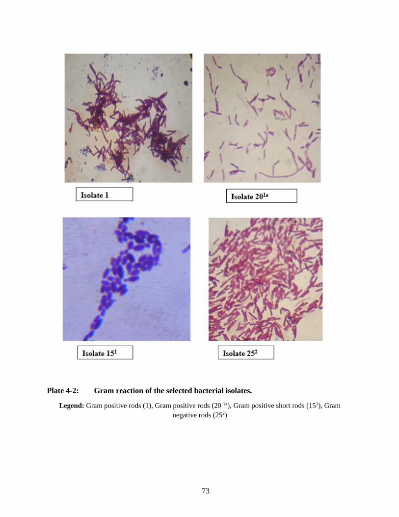
73

Plate 4-2: Gram reaction of the selected bacterial isolates.

Legend: Gram positive rods (1), Gram positive rods (20 1a), Gram positive short rods (151), Gram

negative rods (252)

74

4.3.2 Biochemical tests of the isolates

Results for the various biochemical assays namely, catalase test, fluorescent test, indole test,

starch hydrolysis, motility test, triple iron sugar utilization test, gelatine hydrolysis and hydrogen

sulphide gas production are shown on Table 4-8. Motility test done on SIM medium showed that

some of the isolates were motile with the presence of flagella. Isolates 5, 172, 181, 191and 252

were negative for motility test.

The ability of the isolates to excrete intracellular enzymes was determined through tests on

catalase reaction. Catalase test revealed that isolates 1, 5, 6, 8, 92, 11, 14, 151, 16, 172, 201a, 252

and 271 were positive with the ability for production of hydrogen peroxide as an end product of

oxidation of sugars.

All isolates were positive for Triple Iron Sugar utilization test indicating the ability of the

isolates to ferment glucose and produce a lot of mixed acids as end products of fermentation

(plate 4-3). The medium used, (triple sugar iron agar) is formulated to differentiate bacteria based

on the glucose, lactose and sucrose fermentation (Dhadse et al., 2012; Issazadeh et al., 2013).

The medium is prepared as a shallow agar slant with deep butt, this provides both the aerobic and

anaerobic growth environment. Therefore, the bacteria that are able to ferment glucose and

lactose and/or sucrose were able to turn the medium yellow throughout. Since lactose and

sucrose concentrations are more than that of glucose, both the butt and slant remained yellow

after 24 hours. An organism that does not ferment any of the carbohydrates but utilizes animal

proteins will alkalinize the medium and turn it red. If the organism can use the proteins

aerobically and anaerobically, both the slant and butt will appear red. An obligate aerobe will

turn only the slant red (Amon et al., 2007; Chen et al., 2008). The ability to produce hydrogen

75

sulphide gas is the main function of anaerobic respiration during biogas production (Norrell and

Messley, 1996).

Indole generation by reductive deamination from tryptophan via the intermediate molecule

indole pyruvic acid was tested for the isolates. Tryptophanase enzyme catalyzes the deamination

reaction, during which the amine (-NH2) group of the tryptophan molecule was removed and

final products of the reaction are indole, pyruvic acid, ammonia (NH3), hydrogen sulphide and

energy. The test was performed to show the ability of bacteria to split the amino acid tryptophan

to indole, pyruvic acid and ammonia with the help of tryptophanase enzyme. Positive for indole

test represented the bacterial isolates which were able to act on amino acids by causing

deamination and hydrolysis leading to the formation of pyruvic acid and ammonia. Pyruvic acid

and ammonia are precursors for methane and CO2 production, the main function of

methanogenic bacteria. The negative results showed that isolates were unable to produce indole

as a result of amino acid tryptophan breakdown attributed to lack of tryptophanase in the cell

(Rezwan et al., 2004). The presence of indole can be detected by the addition of Kovacs’ reagent

which reacts with the indole, producing a bright red compound on the surface of the medium. All

isolates were negative for this test but positive for hydrogen sulphide gas prodcution. The test is

important in differentiating members of family Enterobacteriaceae and genus bacillus (Prescott,

2002).

The starch molecule consists of two constituents: amylose, a straight chain polymer of 200 to

300 glucose units, and amylopectin, a larger branched polymer with phosphate groups. Thus,

bacteria that hydrolyze starch produce amylase enzyme that yield molecules of maltose, glucose

and dextrin. Most isolates were positive for the test except isolate 5, 10, 14, 151, 171, 261 and 262

were negative for the test (Table 4-8). 1, 4, 6, 133, 14, 151, 252, 261, and 31 were negative for

76

extracellular gelatinase enzyme. Starch hydrolysis test is used to differentiate bacteria based on

their ability to hydrolyze starch with the enzyme a-amylase or oligo-l, 6-glucosidase, starch is a

polysaccharide consisting of a- D-glucose subunits that exists in two forms amylose (straight

chain polymer) and amylopectin (a larger branched polymer with phosphate groups). Since

starch is too large to pass through bacterial membrane, these enzymes are needed to hydrolyze it

into smaller fragments of glucose molecules making it available for bacteria uptake (Harold,

2002). Therefore, when the bacteria that produce these enzymes are cultivated on starch agar,

they hydrolyze the starch around the area of growth. But since both starch and its sugar subunits

are invisible in the medium, iodine reagent is used to detect the presence or absence of starch in

the around the bacterial growth. Iodine reacts with starch and produces a blue or dark brown

color; therefore, any microbial starch hydrolysis was revealed as a clear zone surrounding the

growth (Cappuccino and Sherman, 2001; Joanne et al., 2016).

Gelatin is a collagenous protein a component of animal connective tissues. Gelatin hydrolysis is

a test that was used to detect the ability of the isolates to produce proteolytic enzyme (gelatinase)

which causes the breakdown of this complex protein derivative to polypeptides. These

polypeptides are further converted into single amino acids that bacteria can easily use for their

metabolic process. Therefore, that hydrolyzed gelatin indicated the presence of gelatinase

enzymes. This test is used to identify and differentiate different species of Bacillus, Clostridium,

Pseudomonas and family Enterobacteriaceae (Prescott, 2002).

The characterization of the bacterial isolates by fluorescent technique, depends on the response

of a target, detailing the fluorescence intensity as a function of both excitation and emission

wavelength, that is provided by an Excitation-Emission Matrix (EEM). An EEM is generated by

recording multiple emission spectra from the target as the excitation wavelength is incremented

77

across a broad range. All isolates showed positive fluorescence apart from 10 and 181 which

were negative.

Plate 4-3: Starch Hydrolysis test (1), Triple Sugar iron test (2) as part of biochemical

tests carried out.

Legend: C-control, -ve-negative, +ve- positive, S_P- slant positive, B_pP-butt partial positive, S+B_P- slant plus butt

positive

78

Table 4-8: Biochemical characteristics of bacterial isolates

TSI

Isolate# Starch Catalase Indole Motility Gelatin Butt Slant Fluorescence H2S

1 + + - + - ++ ++ + +

2 + - - + + ++ ++ ++ +

31 + - - + + ++ ++ ++ +

32 - + - + - ++ ++ + -

4 + + - - - ++ ++ + +

5 - + - - + ++ ++ + +

6 + + - + - +++ ++ ++ +

7 + + - + + ++ +++ + +

8 + + - + + ++ ++ + +

92 + + - + + ++ ++ + +

93a + + - + + + + + + + +

93b + + + + + + + + + + +

10 + + + + + +++ ++ - +

11 + + - + + ++ ++ ++ +

12 + - - + + ++ ++ + +

132 + - - - + ++ +++ + -

133 + - - + - +++ +++ ++ +

14 - + - + - ++ +++ + -

151 - + - - - ++ ++ + +

16 + + - + + ++ ++ + +

171 + - - + + +++ +++ +++ +

172 + + - - + ++ +++ ++ +

181 + + - + + ++ + - -

182 + - - + + + +++ + +

191 + - - - + + +++ + +

201a + + - + + ++ ++ ++ +

252 + + - - - +++ +++ + +

261 - - - + - ++ ++ ++ +

262 - - - + + ++ ++ +++ +

271 + + - + + ++ ++ ++ +

282 + - - + + ++ +++ + +

31 + - - + + ++ ++ ++ +

Key: (+) Positive/ less colour, (-) Negative, (++) partial colour (+++) intense colour and H2S: Hydrogen Sulphide gas.

79

4.3.3 Molecular characterization

4.3.3.1 PCR amplification of 16s rDNA genes from isolates

Genomic DNA was extracted from all the selected 31 isolates using the phenol/chloroform

method. Amplification of 16S rDNA gene with bacterial universal primers bac 8F and bac

1492R (Hogg and Lehane, 1999) yielded an amplification product of approximately 1500 bp as

shown in Plate 4-4. The amplicons were then stained with ethidium bromide and visualised

under UV light on 1 % agarose gel.

Plate 4-4: PCR amplified 16S rRNA products from representative isolates using

universal primers bac 8F and bac 1492R

Legend: Lanes 1(93b*), 2(133*), 3(181*), 4(252 *), 5(262*), 6(151*), 7(182*), 8(32*), 9(201a*), 10(171*) and (M*) M-

1500 bp Molecular marker size

*The figures within the brackets are the isolate numbers

4.3.3.2 Restriction analysis

The restriction enzyme analysis provided an initial clustering of strains into six groups with three

or more members with the same restriction profile. Fragment restriction using RsaI produced six

clusters of the isolates which were generated based on fragment sizes as illustrated in Plate 4-5.

80

Plate 4-5 Restriction products as generated by Rsa I digestion run in 1.5% (W/V)

agarose gel.

Legend: Lanes 1(181*), 2(262 *), 3(15*), 4(201a *), 5(171*), 6(133*), (C*) negative control and (M*) M-1500 bp

Molecular marker size

*The figures within the brackets are the isolate numbers

The amplification of ribosomal DNA restriction analysis (ARDRA) was carried out using this

enzyme. The restriction fragment Cluster profiles obtained from isolates showed patterns with

distinct similarities allowing distinguishing six different groups. These were isolates 1, 2, 3, 5

and 6; which were clustered together generating fragments ranges 300-400bp; isolates 3, 4, 5,

and 6 clustered to generate fragments ranges 400-500bp: isolate 4 generated fragment range 500-

600bp; isolates 4, 5 and 6 were clustered together generating fragments range 600–700bp. Isolate

3 had one restricted fragment of 800-900bp. Finally isolates 1 and 2 were clustered together

generating fragments range 900–1000bp. Sequences of PCR fragments from isolates were in

close agreement with the phylogenetic correlations predicted with the ARDRA approach.

ARDRA thus provided a quick assessment of the diversity in a strain collection.

4.3.3.3 Phylogenetic analysis of the sequences

Though a total of 20 isolates were sequenced, only 16 could be placed into the phylogenetic

trees. The rest were not placed into the tree either because of they had too low an identity to

allow for sensible alignment or they had sequence of less than 320 base pairs according to

81

Rezwan et al., 2004. The taxonomic classification of the isolates performed using morphological

characteristics, biochemical tests and 16S ribosomal RNA sequences of their genomic DNA

placed the isolates to the genera Bacillus, Lysinibacillus, Lactobacillus, Ralstonia, Myroides and

Providencia. Bacilli are described as aerobic or facultative anaerobic; rod shaped, Gram positive,

motile, flagellated bacteria that belongs to the division Firmicutes with varying ecological

diversity. They are most commonly found in soil, waste water, dust, milk and plant surfaces.

Different bacillus species have been described including bacillus subtilis, which supports plant

growth by producing antibiotics that kill other harmful microorganism that may harm the plant

(Lin et al., 2011) bacillus cereus, Bacillus licheniformis and Bacillus tequilensis have been

associated with food spoilage and poisoning.

BLAST analysis of the partial sequences (Table 3) showed that 81.25% were from the genus

Bacillus within the Firmicutes in the domain bacteria with similarities of between 70 and 100%.

Among these were Bacillus subtilis, Bacillus licheniformis, Lactobacillus casei and Bacillus

methylotrophicus. Five isolates from the bacillus group belonged to genus Lysinibacillus sp. with

percentage similarities between 95 and 97. Three isolates had 6.25% each and belonged to the

genera Ralstonia (isolate 32), Providencia (isolate 11) and Myroides (32) with similarities of 77,

96 and 98%, respectively.

Thirteen isolates were clustered into genus Bacillus sp., in the phylogenetic analysis with isolate

93b being closely related to B. subtilis (HQ844623) strain while isolates 201a, 171 and 7 closely

related to B. methylotrophicus (HQ831395). Isolate 10 was grouped together with Bacillus

tequilensis. Isolate 31 was clustered together with B. licheniformis (KJ206991) while isolates

132, 252, 15, 262 and 182 were closely related to Lysinibacillus sp. (KM187000). Isolate 191 was

clustered together with L. casei (KU324896). The study also showed that three isolates including

82

32, 181 and 4 closely related to Ralstonia pickettii (KT354249), Providencia rettgeri (GU193984)

and Myroides odoratimimus (KT597536), respectively as illustrated in Figure 4-4. Isolates 4,

171, 181, 182, 191, 201a, 252, 262 and 31 were isolated from brewing line sample while isolates 32,

7, 93b, 10, 13 and 151, were from the mixing point (Figure3-1).

From the detailed BLAST analysis, the genus Bacillus were found to be the most prominent

indicating a possibility of this group playing an important role in biogas production process as

discussed by Horváth et al., (2016); Kröber et al., (2009) and Li et al., (2013). This compares to

the results obtained by Rabah et al., (2010) using abattoir waste as the inoculum. The results are

also in line with that of Onwuliri et al., (2016) in which Bacillus, Yersinia, and Pseudomonas

species were found to be responsible for biogas production from cow dung. Bacilli are described

as aerobic or facultative anaerobic; rod shaped, Gram positive, motile, flagellated bacteria, either

catalase positive that belongs to the division Firmicutes with varying ecological diversity. They

are most commonly found in soil, wastewater, milk, dust, and plant surfaces.

Phylogenetic analysis of isolate 93b suggested that it was closely related to Bacillus subtilis with

94% rDNA sequence analysis similarity. The morphological and biochemical tests supported this

since the isolate was Gram positive rod, catalase, starch hydrolysis and sugar fermentation

positive and did produce hydrogen sulphide gas. Bacillus subtilis is widely used in the industrial

production of amino acids, recombinant proteins and fine chemicals (Straight et al., 2006). It is

also known for generation of bioenergy, production of industrial metabolites and bioremediation

(Novak et al., 2013; Porwal et al., 2015). Isolates 201a, 171 and 7 closely related to Bacillus

methylotrophicus with 97-98% rDNA sequence analysis similarity (Table 4-9).

83

Table 4-9: BLAST analysis results of the isolates nearest neighbours in the data bank and their percentage relatedness.

Isolate Next Neighbour Accession

Number % similarity

93b-(bac 8F) Bacillus subtilis strain AIMST 7.Os.2 HQ844623.1 94

Bacillus licheniformis strain BNR143 KT074465.1 94

Bacillus tequilensis strain HS10 KP743123.1 94

181-(bac 8F) Bacillus thuringiensis serovar indiana strain HD521 CP010106.1 100

Bacillus cereus strain S2-8 JF838294.1 100

Bacillus anthracis strain Ames_BA1004 CP009981.1 100

252-(bac 8F) Bacillus sp. MSB1-25E KT030900.1 96

Lysinibacillus fusiformis strain L13 KU179364.1 96

Lysinibacillus sphaericus strain C2-37c-8 JX517244.1 96

Lysinibacillus xylanilyticus strain 11W6RMR3-2 KT728728.1 96

262-(bac 8F) Lysinibacillus boronitolerans strain KnMuC3-2 KF032677.1 97

Lysinibacillus sp. BFE17K1 KM187000.1 97

15-(bac 8F) Lysinibacillus sp. DB14515 KP670240.1 97

Lysinibacillus xylanilyticus strain RD_AZIDI_12 KU597545.1 97

182-(bac 8F) Lysinibacillus xylanilyticus strain MA KT030900.1 95

Lysinibacillus fusiformis strain L13 KU179364.1 95

201a-(bac 8F) Bacillus amyloliquefaciens strain Y1 KJ616752.1 97

Bacillus methylotrophicus strain Nk5-1 HQ831395.1 97

Bacillus subtilis strain yxw4 KF278950.1 97

Bacillus methylotrophicus strain NMTD14 HQ844484.1 97

171-(bac 8F) Lysinibacillus boronitolerans strain KtTA1-2 KF025654.1 97

Lysinibacillus sp. Je33-2 HF563553.1 97

10-(bac 8F) Bacillus subtilis strain F111 HQ647257.1 98

Bacillus tequilensis strain ADIP3 KF732811.2 98

84

Geobacillus sp. CRRI-HN-1 JQ695928.1 98

32-(bac 8F) Ralstonia mannitolilytica strain 4903 KT933223.1 77

Ralstonia pickettii KT354249.1 77

Uncultured bacterium clone Ap.ba-F-DM-HN-1-46 KT354249.1 77

11-(bac 8F) Providencia rettgeri strain IITRP2 GU193984.1 96

Uncultured Providencia sp. clone F2jun.39 GQ417423.1 96

Uncultured bacterium clone PB16 GU166190.1 96

16-(bac 8F) Bacillus licheniformis strain RTS EF644417.1 95

Bacillus sp. J26 JF783986.1 95

Bacillus tequilensis strain EB-95 KU258071.1 95

Bacillus subtilis strain 1201 EU982509.1 95

191-(bac 8F) Lactobacillus casei strain L1 KM350161.1 95

Lactobacillus casei strain MSJ1 KU324896.1 95

Lactobacillus casei strain EM2 KM350160.1 95

32-(bac 8F) Myroides odoratimimus strain LZ1306-2-5 KT597536.1 98

Myroides odoratimimus strain YRL08 EU373415.1 98

7-(bac 8F) Bacillus amyloliquefaciens subsp. plantarum strain L09 JN700139.1 98

Bacillus methylotrophicus strain CR1 KP851947.1 98

Bacillus subtilis strain EPP2 2 JQ308548.1 98

31-(bac 8F) Bacillus licheniformis strain R2 KJ206991.1 70

Bacillus licheniformis strain SMR1 KF600749.1 70

Bacillus subtilis strain VJJS-01 DQ872516.1 70

85

Figure 4-4: Phylogenetic analysis of 16S rDNA gene sequences using the Maximum Likelihood

method based on the Tamura-Nei model (2007).

The tree is drawn to scale, with branch lengths measured in the number of substitutions per site. The analysis

involved 29 nucleotide sequences. The gene sequence of Trichoderma sp. (HQ630962.1) was used as an out-group.

Isolate 133 (8F)

Isolate 252 (8F)

Isolate 15 (8F)

Isolate 262 (8F)

Isolate 182 (8F)

Lysinibacillus sp.(KM187000)

Lysinibacillus xylanilyticus (KU597545)

Bacillus sp.(LN907825)

Ralstonia pickettii (KT354249)

Ralstonia mannitolilytica (KT933223)

Isolate 32 (8F)

Isolate 181 (8F)

Providencia rettgeri (GU193984)

Isolate 4 (8F)

Myroides odoratimimus (KT597536)

Isolate 191 (8F)

Lactobacillus casei (KU324896)

Bacillus licheniformis (KJ206991)

Isolate 31 (8F)

Isolate 10 (8F)

Bacillus tequilensis (KF732811)

Bacillus sp.(JF783986)

Bacillus methylotrophicus (HQ831395)

Isolate 201a (8F)

Isolate 171 (8F)

Isolate 7 (8F)

Isolate 93b (8F)

Bacillus subtilis (HQ844623)

Trichoderma sp.(HQ630962)

0.2

86

Phenotypic characteristics revealed that Bacillus methylotrophicus is Gram positive, rod shaped,

endospore former, catalase positive and motile (Table 4-7). Various methylotrophs have also

been described, including methanotrophs, some of which are obligate methane users, those that

use methanol and a few that are able to grow on carbon containing compounds (Dedysh et al.,

2005).

Morphological and biochemical signatures of isolate 10 indicated that it was highly closely

related to Bacillus tequilensis, with 98% rDNA sequence analysis similarity. It’s a Gram positive

motile rod, indole and catalase positive, liquefied gelatine, hydrolysed starch and fermented all

three sugars through TSI test. It was first isolated from 2000-year-old tomb but generally it’s

found in the soil and most environmental samples, (Gatson et al., 2006; Rooney et al., 2009).

Studies shows Bacillus tequilensis can produce an enzyme pectinase with many industrial

applications such as pre-treatment of waste water, (Shah et al., 2013). Isolate 31 was closely

related to Bacillus licheniformis with 16SrDNA sequence analysis of 70% and was Gram

positive, motile rod, catalase positive, aerobic or facultative anaerobic. Bacillus licheniformis,

has been associated with spoilage of food, under different clinical conditions (Ghani et al.,

2013). The rapid development of industrial enzymology and fermentation technology have

allowed the exploitation of this species for production of different enzymes.

Lysinibacilli are diverse group with different species, they are naturally found in various

environments including farming soil and factory wastewater. Many Lysinibacillus species have

been described including; Lysinibacillus boronitolerans, and also reclassified Bacillus sphaericus

and Bacillus fusiformis to the genus Lysinibacillus. Several other species have also been added

to this genus, Lysinibacillus parviboronicapiens, (Miwa et al., 2009). Sequence analysis by

87

BLAST search system on the NCBI website and phylogenetic analysis (Figure 1) showed that

the isolates 132, 252, 15, 262 and 182 was phylogenetically most closely related to Lysinibacillus

sp (KM187000) with 95-99% rDNA sequence similarity (Table4- 9). These isolates adhere to the

phenotypic and biochemical characteristics of Lysinibacillus sp which is Gram positive, rod

shaped motile or non-motile bacteria and were positive for starch hydrolysis, sugar fermentation

and were negative for indole production (Table 4-8).

Isolate 191 displayed the typical characteristics and biochemical properties similar to

Lactobacillus casei. It was Gram positive, non-motile, rod shaped catalase negative, and

facultative anaerobic. It is believed to be a normal inhabitant of the oral cavity and the digestive

tract in humans. It has been found to be also involved in the reduction of Chemical Oxygen

Demand and colour from dark effluent, (Shibu et al., 1999). Sequence analysis by BLAST search

systems on NCBI website showed that the isolate 191 was phylogenetically most closely related

to Lactobacillus casei with 95 % rDNA sequence similarity (Table 4-9). Ralstonia pickettii

belongs to family Burkholderiaceae and was first isolated from soil and water it can degrade

various chlorophenol compounds, aromatic hydrocarbons 2,4-dichlorophenoxyacetic acid and

pentacyclictriterpeniod compounds, (Seal et al., 1993).

The morphological and biochemical signatures for isolate 32 indicated that they are closely

related to Ralstonia pickettii. It was Gram negative and motile rod, starch hydrolysis, indole,

gelatin liquefaction and hydrogen sulphide production negative and catalase positive and

fermented sugars through TSI test. The 16S rDNA sequence analysis suggested the isolate 32 is

phylogenetically closely related to Ralstonia pickettii with 77% sequence similarity (Table 4-9).

88

Members of genus Providencia are Gram negative motile rods belonging to family

Enterobacteriaceae, they are positive for catalase and acid production from glucose fermentation,

without production of H2S gas. They are mostly isolated from water and clinical (urine, faeces,

blood, wounds and throat) human and animal samples, (Holt et al., 1994). Morphological and

biochemical characteristics showed that isolate 181 was closely related to Providencia rettgeri

being a Gram- negative, motile rods, catalase, starch hydrolysis positive and was negative for

indole and hydrogen sulphide gas production, (Table 4-8). Sequence analysis by BLAST search

systems on NCBI website showed that the isolate 181 was phylogenetically most closely related

to Providencia rettgeri with 96% rDNA sequence similarity (Table 4-9).

Myroides species, which are formerly classified as Flavobacteriun odoratum, are Gram-negative,

non-fermentative, obligately aerobic, yellow-pigmented, non-motile rods and are commonly

found in the soil and water. This genus of Myroides comprises of, Myroides odoratus and

Myroides odoratimimus, (Vancanneyt et al., 1996). Isolate 4 displayed the typical characteristics

and biochemical properties similar to Myroides odoratimimus. It was Gram negative, non-motile

and rod shaped, catalase, TSI, starch hydrolysis and hydrogen sulphide gas positive and was

negative for indole, gelatin liquefaction. It was closely related to Myroides odoratimimus with

98% rDNA sequence analysis similarity (Table 4-9).

4.4 Optimization of biogas from isolated strains

4.4.1 Effect of temperature and pH on the quality of methane production

The pH ranges of brewery wastewater is reported as 6.5 to 8.2 (Caliskan et al., 2014;

Janhoappliedm et al., 2009; Zheng et al., 2015). The study considered pH values of 6, 7.2 and 8

in order to investigate the effect of pH on the growth of the bacteria which has a direct impact on

89

the concentration of methane gas produced by the different isolates (Ward et al., 2008). The low

pH of 6 and temperature of 30°C, and high pH of 8 and temperature 40°C, may have inhibited

the growth of some isolates, resulting in low concentrations of the methane produced (Figure 4-

5). However, production of methane at low pH is essential for digestion to progress from the

anaerobic acid phase to the methane production phase. Presence of isolate 252, 262 and 201a

which were acid tolerant is consistent with literature (Ladapo and Barlaz, 1997). At pH 7.2, most

of the isolates were able to adjust and increase in numbers especially at temperatures between 35

and 37°C. The isolates observed floating in the digesters could indicate a possibility of death for

these isolates as they could not adapt easily to the high pH and temperature of 40°C.

Table 4-10 shows the means of the quality of methane gas produced by different isolates.

Generally, 88.9% of the isolates had the highest percentage quality of methane gas at the

temperature range of 35 ºC - 37 ºC for all the pH ranges. However, the quality produced by

isolate 151 at temperature 30 ºC and pH 8 was significantly different from that produced at higher

temperatures and low pH. This isolate was observed to have the highest concentration at this pH

and temperature and was significantly different (p<0.001) from that produced by the other

isolates as illustrated in Figures 4-5, 4-6, 4-7, 4-8 and 4-9. The results didn’t show any

significance difference in the volume of the gas generated for different temperatures, although

slight variations were observed with temperatures 30 ºC and 40 ºC recording the highest volume

of gas but low in quality. Similarly, temperatures 35 ºC and 37 ºC had the lowest volumes of gas

produced with better quality with high methane concentrations as indicated in Figure 4.6.

90

Figure 4-5: Effect of temperature and pH on the quality of the methane produced at OD

600 nm

91

Table 4-10: Means for quality of methane gas produced by different isolates

pH Temperature

(°C) 15^1 17^1 18^1 18^2 20^1a 25^2 26^2 3^2 9^3b

6.0 30 0.52±0.02cd 0.72±0.02d 0.29±0.07a 0.48±0.02c 0.33±0a 0.31±0b 0.41±0.03b 0.29±ab 0.24±0.02a

6.0 35 0.64±0.05d 0.93±0.03e 0.62±0.07c 0.67±0.07d 0.69±0.06d 0.5±0.03cd 0.79±0.03h 0.28±0a 0.74±0.01bc

6.0 37 0.38±0.01abc 1.12±0.02f 0.49±0.03b 0.42±0.03bc 0.58±0c 0.47±0.01c 0.29±0a 0.29±0.01ab 0.35±0a

6.0 40 0.33±0.01ab 0.34±0.01b 0.23±0a 0.26±0a 0.28±0a 0.3±0b 0.25±0a 0.33±0ab 0.29±0.01a

7.2 30 0.32±0.01ab 0.21±0a 0.33±0.01a 0.73±0d 0.48±0.02b 0.21±0a 0.44±0.06bc 0.38±0.01bc 0.43±0.04a

7.2 35 0.24±0.02a 0.33±0.01b 0.43±0.01b 1.12±0.03f 0.48±0.02b 0.21±0.01a 0.47±0.03bcd 0.43±0.01c 0.63±0.04b

7.2 37 0.44±0.02bc 0.51±0.08c 0.72±0.08d 1.15±0.03f 0.5±0b 0.78±0.01e 0.5±0cde 0.6±0d 0.62±0b

7.2 40 0.47±0.01bc 0.25±0.02ab 0.52±0bc 0.75±0.02d 1.3±0f 0.76±0.02e 0.51±0.04cde 0.59±0.09d 0.61±0.01b

8.0 30 0.86±0.14e 0.75±0.01d 1.1±0e 0.97±0.08e 0.55±0bc 0.55±0d 0.55±0.02def 0.52±0.03d 0.83±0.19c

8.0 35 0.45±0.01bc 2.3±0h 2.2±0f 0.77±0d 0.77±0e 0.52±0.03d 0.58±0ef 0.73±0e 2.3±0d

8.0 37 0.42±0bc 2.1±0g 1.08±0.01e 0.42±0bc 0.7±0de 0.51±0.01cd 0.66±0.02g 2.1±0f 0.7±0bc

8.0 40 0.37±0.02ab 0.71±0.05d 1.1±0e 0.34±0.02ab 0.5±0.03b 0.51±0.01cd 0.63±0fg 0.77±0e 0.77±0bc

LSD 0.133 0.093 0.104 0.107 0.069 0.045 0.080 0.092 0.189

CV% 17.1 6.3 7.8 9.2 6.6 5.5 9.2 7.8 14.4

Note: LSD means least significant difference; CV means coefficient of variance

92

0.0105

0.0110

0.0115

0.0120

0.0125

0.0130

0.0135

15^

1

17^

1

18^

1

18^

2

20^

1a

25^

2

26^

2

3^2

9^3

b

15^

1

17^

1

18^

1

18^

2

20^

1a

25^

2

26^

2

3^2

9^3

b

15^

1

17^

1

18^

1

18^

2

20^

1a

25^

2

26^

2

3^2

9^3

b

15^

1

17^

1

18^

1

18^

2

20^

1a

25^

2

26^

2

3^2

9^3

b

30 35 37 40

To

tal v

olu

me o

f g

as in

lit

res

Temperature in oC

6.0

7.2

8.0

Figure 4-6: Effect of temperature and pH on the quantity of gas produced

93

Figure 4-7: Methane quality at pH 6

Figure 4-8: Methane quality at pH 7.2

94

0.0

0.5

1.0

1.5

2.0

2.5

30 35 37 40

Met

han

e q

ual

ity i

n %

Temperature in oC

15^1

17^1

18^1

18^2

20^1a

25^2

26^2

3^2

9^3b

Figure 4-9: Methane quality at pH 8

4.4.2 Growth curves of the isolates at 37ºC

Figure 4-10 shows the sigmoidal shaped curves obtained for the isolates; 32, 93b, 151, 181,182,

201a, 171, 252 and 262. The curves clearly showed different stages of growth, including the lag

phase, exponential phase and the stationary phase. Variation in the lag time for the isolates was

observed for most of the isolates. The growth was not observed during the first 4 hours of

incubation, but increased with increase in incubation period until 6th hour for isolate 93b, and 182,

while isolates 201a, 171, 252, 181,262, 151, increased till the 15th hour, with isolate 32 reaching the

18th hour, after which the growth was either stagnant or decreased as shown in Figure 4-10.

The growth curve of a microbial culture for the nine isolates was used to analyse their population

growth. From the sigmoidal curve obtained Figure 4-10, the growth of most of the isolates could

not be detected during the first four hours. This could be attributed to the lag phase in which the

microorganisms were adapting to the new conditions having been inoculated in a fresh medium

95

and possibly the microorganisms have been injured and required time to recover (Klocke et al.,

2008; Kotsyurbenko, 2005). After the 4th hour the growth of these isolates could be compared to

the exponential phase in which case the growth increased with increase in incubation period. At

this stage the isolates are growing and dividing at the maximal rate possible as they have

adjusted to the new environment and that the microorganisms are dividing and doubling in

number at regular intervals. From Figure 4-10, the curves for most of the isolates rose smoothly

than discrete jumps indicating that the individual isolate divides at a slightly different time. The

population of the microorganism at this stage is uniform with regards to the chemical and

physical properties (Koch, 2001; Panikov, 1995) thus the maximum production of the methane

gas could be linked to this stage. To maximize methane production, the exponential phase could

be pro-longed by using continuous culture system, in which constant environmental conditions

are maintained through continual provision of nutrients and removal of wastes. In this system,

cells are supplied with nutrients and grow at a constant rate.

The decrease in the population growth observed could be attributed to nutrient limitation and

accumulation of toxic waste products, which seems to limit the growth of many anaerobic

cultures, (Cooper, 1991) although other factors could inhibit their growth.

96

8

8.5

9

9.5

10

10.5

0 1 2 4 6 15 18 22 24 28

Log N

(t)

Time (hours)

3^2

9^3b

15^1

17^1

18^1

18^2

20^1a

25^2

26^2

Figure 4-7: Monitored growth of the isolates at temperature 37⁰C

4.4.3 Comparing growth Models for predicting microbial growth.

Table 4-12 shows the growth parameters as estimated by the Gompertz and logistic models for

the growth curves of isolates 32, 93b, 252,171,182, and 201a, plotted with the log of N values as

shown in Figure 4-11. Both models provided the values that could be expected for growth

parameters of the selected six microorganism.

97

Table 4-11: Estimated growth parameters and their 95%confidence limits of fit obtained with growth curves for isolates32,

93b, 252, 171, 182 and 201a

Isolate Growth Model Initial Concentration (No) Asymptote

A(cells)

Growth

rate(µmax)cells h-1 Lag time (λ)( h)

Akaike information

criterion (AIC) r2 SSE

32 Gompertz 9.204 9.845 1.402 1.478 x 101 -46.783 0.998 0.002

(9.191 - 9.211) (9.832 - 9.854) (0.222 - 1) (13.717 - 14.715)

Logistic 9.204 9.845 0.9519 1.468 x 101 -46.982 0.985 0.014

(9.191 - 9.218) (9.829 - 9.854) (0.683 - 1.532) (14.545 - 14.809)

93b Gompertz 9.204 9.9 0.743 4.702 -26.253 0.986 0.016

(9.141 - 9.232) (9.863 - 9.933) (0.355 - 2.680) (3.763 - 4.725)

Logistic 9.204 9.9 1.548 5.468 -25.252 0.979 0.026

(9.158 - 9.227) (9.863 - 9.933) (0.397 - 1.890) (3.982 - 5.588)

252 Gompertz 9.204 9.916 7.05 x 10-1 4.719 -15.212 0.962 0.047

(9.144 - 9.252) (9.880 - 9.980) (0.257 - 2.217) (3.171 - 4.809)

Logistic 9.204 9.916 1.64 5.523 -15.212 0.944 0.087

(9.145 - 9.258) (9.876 - 9.979) (0.245 - 2.014) (3.183 - 5.620)

171 Gompertz 8.901 9.733 0.238 4.733 -29.625 0.993 0.011

(8.865 - 8.930) (9.704 - 9.759) (0.117 - 0.637) (3.648 - 5.599)

98

Logistic 8.903 9.733 0.971 5.693 -29.588 0.981 0.031

(8.865 - 8.935) (9.705 - 9.766) (0.167 - 1.939) (4.252 - 5.873)

182 Gompertz 8.903 9.904 0.977 4.765 -17.743 0.985 0.037

(8.799 - 8.955) (9.842 - 9.951) (0.534 - 2.549) (3.831 - 4.884)

Logistic 8.903 9.904 2.322 5.545 -17.742 0.983 0.038

(8.850 - 8.942) (9.841 - 9.951) (0.443 - 2.737) (3.976 - 5.647)

201a Gompertz 9.204 9.87 0.797 4.469 -20.101 0.973 0.029

(9.123 - 9.250) (9.836 - 9.916) (0.357 - 2.592) (3.760 - 4.782)

Logistic 9.204 9.87 1.567 5.366 -20.001 0.937 0.069

(9.133 - 9.241) (9.842 - 9.924) (0.364 - 2.036) (5.733 - 5.633)

99

Figure 4-8: Growth curve for isolate 32 at 37C, pH 7.2 fitted with the Gompertz and

logistic model

Both models provided a high goodness of fit (R2> 0.93) for all growth curves for three isolates,

in approximately 33% of the cases. The differences between the Gompertz and logistic models

were not significant, which is in line with the findings of Longhi et al., 2013. However,

Gompertz model was accepted in 75% of the remaining cases based on the AIC values and also

supported by the R2> 0.95 values and small RSS values (Table 4-12). For all the isolates,

Gompertz and Logistic models gave different estimates of the growth parameters. For isolate 32

the models could not accurately estimate the growth parameters, for instance the lag time was

Asymptote A

(Maximum population)

Lag time

100

over estimated to close to 14.78 hours by Gompertz and 14.68 hours for logistic model, Figure 4-

11. The estimated growth rate of 1.402 cells per hour by Gompertz model was outside the

confidence interval limits. However, logistic model was found to have a lower AIC value as

compared to Gompertz model, and the r2 value of 0.986 was also lower as compared to 0.998

given by the Gompertz model, although based on the AIC value, the logistic model is likely to be

correct.

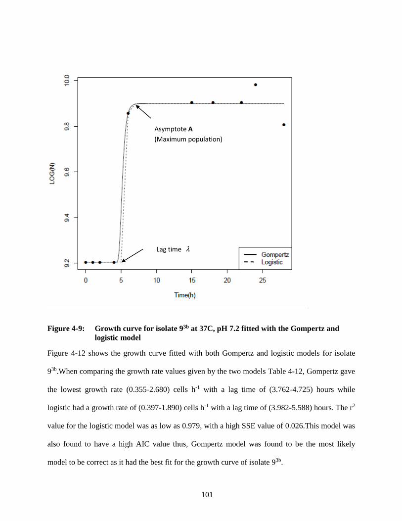
101

Figure 4-9: Growth curve for isolate 93b at 37C, pH 7.2 fitted with the Gompertz and

logistic model

Figure 4-12 shows the growth curve fitted with both Gompertz and logistic models for isolate

93b.When comparing the growth rate values given by the two models Table 4-12, Gompertz gave

the lowest growth rate (0.355-2.680) cells h-1 with a lag time of (3.762-4.725) hours while

logistic had a growth rate of (0.397-1.890) cells h-1 with a lag time of (3.982-5.588) hours. The r2

value for the logistic model was as low as 0.979, with a high SSE value of 0.026.This model was

also found to have a high AIC value thus, Gompertz model was found to be the most likely

model to be correct as it had the best fit for the growth curve of isolate 93b.

Lag time

Asymptote A

(Maximum population)

102

Figure 4-10: Growth curve for isolate 171 at 37C, pH 7.2 fitted with the Gompertz and

logistic model

Gompertz model had the lowest values for the estimated growth parameters as (0.117-0.637)

cells h-1 for growth rate and lag time of (3.648-5.599) hours as compared to (0.167-1.940) cells h-

1 and (4.252-5.873) hours respectively for logistic model.(Figure 4-13).The AIC value and RSS

value for this model were also observed to be lower. However, the r2 value for all the models

were below 0.995. Basing on the AIC value, the Gompertz model was found to be the most

likely to be correct.

Lag time

Asymptote A

(Maximum population)

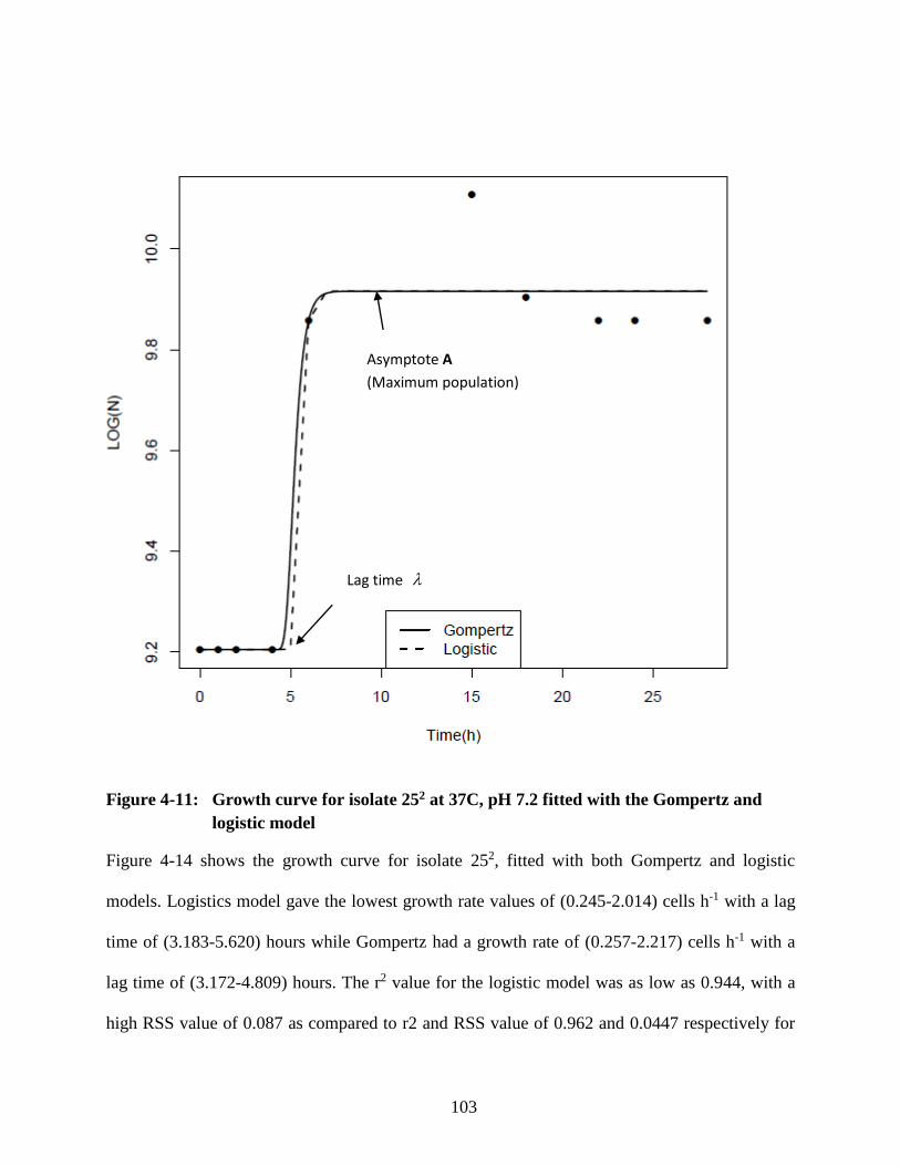
103

Figure 4-11: Growth curve for isolate 252 at 37C, pH 7.2 fitted with the Gompertz and

logistic model

Figure 4-14 shows the growth curve for isolate 252, fitted with both Gompertz and logistic

models. Logistics model gave the lowest growth rate values of (0.245-2.014) cells h-1 with a lag

time of (3.183-5.620) hours while Gompertz had a growth rate of (0.257-2.217) cells h-1 with a

lag time of (3.172-4.809) hours. The r2 value for the logistic model was as low as 0.944, with a

high RSS value of 0.087 as compared to r2 and RSS value of 0.962 and 0.0447 respectively for

Lag time

Asymptote A

(Maximum population)

104

the Gompertz model. Gompertz model however had a lower AIC value thus, it was found to be

the most likely model to be correct for isolate 252.

Figure 4-12: Growth curve for isolate 182 at 37C, pH 7.2 fitted with the Gompertz and

logistic model

Growth curve for isolate182, fitted with both Gompertz and logistic models Figure 4-15 above

displayed both Logistics model and Gompertz model to estimate relatively similar values for the

growth parameters, Figure 4-15 and Table 4-12.The RSS value of 0.037 for Gompertz and 0.038

for logistic were also observed with little or no difference. The same observation was made for

Lag time

Asymptote A

(Maximum population)

105

the AIC values, thus, both models were likely to be correct although their r2 values were below

0.995 (Table 4-12).

Figure 4-13: Growth curve for isolate 201a at 37C, pH 7.2 fitted with the Gompertz and

logistic model

Figure 4-16 shows the growth curve for isolate201a, fitted with both Gompertz and logistic

models. Gompertz model gave the lowest growth rate values of (0.357-2.592) cells h-1 with a lag

time of (3.760-4.782) hours while Logistic had a growth rate of (0.364-2.036) cells h-1 with a lag

time of (3.733-5.633) hours. The r2 value for the logistic model was as low as 0.937, with a high

RSS value of 0.069 as compared to r2 and RSS value of 0.973 and 0.0029 respectively for the

Lag time

Asymptote A

(Maximum population)

106

Gompertz model. Gompertz model however had a lower AIC value thus, it was found to be the

most likely model to be correct for isolate 201a.

Generally, data on growth curves are necessary to define and construct predictive models in

anaerobic digestion. For reduction of measured data to important growth parameters in microbial

growth, models play an important role as opposed to using linear regression. The lag stages,

slopes and constant growth stages for all the growth curves representing the growth of these

microorganism were in line with, lag, exponential and stationary growth phases as reported in

literature (Esser et al., 2015; Perni et al., 2005; Pla et al., 2015; Zwietering et al., 1990). The lag

time and growth rates for the microorganisms were also different although they were grown in

the same conditions, depicting different adaption times for different microorganisms (Koch,

2001; Panikov, 1995).This information could be useful in the determination of the sludge

retention time for the methanogenesis step in order to allow maximum contact of the feedstock

and the bacterial mass and to minimize transport problems related to toxins with respect to

substrate compounds, intermediate and end products (Y. Chen et al., 2008; Karakashev et al.,

2005).

4.5 Contribution to knowledge

Anaerobic digestion of bio-waste is the most predictable way to produce biogas with high

methane content, which has great potential to replace fossil fuel in various application. The

models presented provides knowledge to describe the growth of the isolated and identified

methanogenic community in a bio-digester as a function of time, hence maximum utilization of

the exponential phase of the microbial growth for production of biogas. This indicates the

practicality of applying Gompertz model to actual anaerobic digestion of brewery waste as a step

107

towards optimal methane production. The specific growth rate and lag time parameters were

obtained from the models. The BI model developed guides on physicochemical parameters to be

maximized to ensure proper levels of COD and BOD for both higher biodegradability ratio for

optimal biogas production and also reduce environmental pollution. The study also provides

information on the characteristics of the brewery wastewater before treatment, thus cautioning

direct discharge to the environment.

108

CHAPTER FIVE

5.0 Conclusions and recommendations

5.1 Conclusions

1. The untreated brewery wastewaters generally had high levels of COD of

50966±20146.67mg/l and BOD of 3403±53.52 mg/l in both industries. The variations

were prominent between industries. These industries have high organic loadings, thus the

demand for environmental investments is high but, the organic material available in

brewery wastes also has very high potential for bioenergy production allowing an

environmentally friendly disposal solution. However, pretreatment prior to the digestion

is necessary for improved biogas production. The low ratio of BOD to COD at the

brewing line and CIP line could have a negative effect on the biogas production thus

anaerobic digestion of the wastewater from these streams separately could be

uneconomical.

2. The study has demonstrated that brewery wastewater harbour diverse bacteria species

with potential biogas production. 31 isolates were obtained; 16 isolates were

characterized and identified. Biochemical properties of some isolates for instance ability

to ferment different sugars, hydrolysis starch, liquefy gelatin, split amino acid tryptophan,

produce catalase enzyme and hydrogen sulphide gas suggests their involvement in biogas

production. Molecular characterization of the bacterial isolates indicates that 50 %

belong to genus Bacillus within the Firmicutes in the domain bacteria, 32 % belong to the

genus Lysinibacillus sp. The genus Ralstonia and Myroides both had 6 % each. Ten (10)

isolates showed identity of 95 - 97 % similarity with the previously known sequences in

109

the GenBank database. Two (2) isolates showed identity of 70 -93 % similarity,

representing novel genera of organisms within brewery waste water.

3. Comparisons of the behavior of the two primary growth models (Gompertz and Logistic)

for different isolates at the same growth conditions showed that Gompertz model was the

best-fitting model. These results provided insight into predicting microbial growth using

proper primary growth predictive model, in anaerobic digestion as a step towards

optimizing methane production.

5.2 Recommendations

The obtained bacterial isolates could be adopted for commercial production of methane but for

full potential, further studies could be undertaken on:

1. Effect of seasonal changes on the quality of the brewery wastewater.

2. Continuous system as opposed to batch system with variation of the substrate

concentration.

3. Unique physiological characteristics of the isolates to be to explore the applicability

and full potential of the isolates.

110

REFERENCES

Adekunle, K. F., & Okolie, J. A. (2015). A Review of Biochemical Process of Anaerobic

Digestion. Scientific Research Publishing Inc., 6(March), 205–212.

http://doi.org/http://dx.doi.org/10.4236/abb.2015.63020

Akpor, O. B., Muchie, M. (2011). Environmental and public health implications of wastewater

quality. African Journal of Biotechnology, 10(13), 2379–2387.

http://doi.org/10.5897/AJB10.1797

Ali Shah, F., Mahmood, Q., Maroof Shah, M., Pervez, A., & Ahmad Asad, S. (2014). Microbial

ecology of anaerobic digesters: The key players of anaerobiosis. The Scientific World

Journal, 2014. http://doi.org/10.1155/2014/183752

Amon, T., Amon, B., Kryvoruchko, V., Machmüller, A., Hopfner-Sixt, K., Bodiroza, V., …

Zollitsch, W. (2007). Methane production through anaerobic digestion of various energy

crops grown in sustainable crop rotations. Bioresource Technology, 98(17), 3204–3212.

http://doi.org/10.1016/j.biortech.2006.07.007

Angelidaki, I., & Ellegaard, L. (2003). Codigestion of manure and organic wastes in centralized

biogas plants: status and future trends. Applied Biochemistry and Biotechnology, 109(1-3),

95–105. http://doi.org/10.1385/ABAB:109:1-3:95

APHA. (2005). Standard methods for the examination of water and wastewater (21st ed.).

Washington, DC.

Appels, L., Baeyens, J., Degrève, J., & Dewil, R. (2008). Principles and potential of the

anaerobic digestion of waste-activated sludge. Progress in Energy and Combustion Science,

111

34(6), 755–781. http://doi.org/10.1016/j.pecs.2008.06.002

Batstone, D. J., Vavilin, V., Keller, J., Angelidaki, I., Kalyuzhnyi, S. ., Pavlostathis, S. ., &

Rozzi, A. (2002). Anaerobic digestion model No 1. Water Science and Technology : A

Journal of the International Association on Water Pollution Research, 45(10).

Bayer, E. A., Belaich, J., Shoham, Y., & Lamed, R. (2004). THE CELLULOSOMES :

Multienzyme Machines for Degradation of Plant Cell Wall Polysaccharides. Ann.

Rev.Microbiol, 58, 521–554. http://doi.org/10.1146/annurev.micro.57.030502.091022

Bergmann, I., Mundt, K., Sontag, M., Baumstark, I., Nettmann, E., & Klocke, M. (2010).

Influence of DNA isolation on Q-PCR-based quantification of methanogenic Archaea in

biogas fermenters. Systematic and Applied Microbiology, 33(2), 78–84.

http://doi.org/10.1016/j.syapm.2009.11.004

Björnsson, L., Murto, M., Jantsch, T. G., & Mattiasson, B. (2001). Evaluation of new methods

for the monitoring of alkalinity, dissolved hydrogen and the microbial community in

anaerobic digestion. Water Research, 35(12), 2833–2840. http://doi.org/10.1016/S0043-

1354(00)00585-6

Budiyono, & Kusworo, T. D. (2011). Biogas Production From Cassava Starch Effluent Using

Microalgae As Biostabilisator. International Journal of Science and Engineering, 2(1), 4–8.

Caliskan, G., Giray, G., Gundogdu, T. K., & Azbar, N. (2014). Anaerobic Biodegradation of

Beer Production Wastewater at a Field Scale and Explotation of Bioenergy Potential of

Other Solid Wastes from Beer Production. International Journal of Renewable Energy and

Biofuels, 2014. http://doi.org/10.5171/2014.664594

112

Cappuccino, J. G., & Sherman, N. ›. (2001). Microbiology: A Laboratory Manual (6th ed.).

Benjamin Cummings.

Chandra, J., & Mani, S. (2011). A study of 2 rapid tests to differentiate Gram positive and Gram

negative aerobic bacteria. Medical and Allied Sciences, 1(2), 84–85.

Chen, C. L., Wu, J. H., & Liu, W. T. (2008). Identification of important microbial populations in

the mesophilic and thermophilic phenol-degrading methanogenic consortia. Water

Research, 42(8-9), 1963–1976. http://doi.org/10.1016/j.watres.2007.11.037

Chen, Y., Cheng, J. J., & Creamer, K. S. (2008). Inhibition of anaerobic digestion process: A

review. Bioresource Technology, 99(10), 4044–4064.

http://doi.org/10.1016/j.biortech.2007.01.057

Cioabla, A., Ionel, I., Dumitrel, G.-A., & Popescu, F. (2012). Comparative study on factors

affecting anaerobic digestion of agricultural vegetal residues. Biotechnology for Biofuels,

5(1), 39. http://doi.org/10.1186/1754-6834-5-39

Cirne, D. G., Lehtomäki, A., Björnsson, L., & Blackall, L. L. (2007). Hydrolysis and microbial

community analyses in two-stage anaerobic digestion of energy crops. Journal of Applied

Microbiology, 103(3), 516–527. http://doi.org/10.1111/j.1365-2672.2006.03270.x

Clarridge, E. J. (2004). Impact of 16S rRNA gene sequence analysis for identification of bacteria

on clinical microbiology and infectious diseases. Clin. Microbiol. Rev., 17(4), 840–862.

http://doi.org/10.1128/CMR.17.4.840

Clemens, J., Trimborn, M., Weiland, P., & Amon, B. (2006). Mitigation of greenhouse gas

emissions by anaerobic digestion of cattle slurry. Agriculture, Ecosystems and Environment,

113

112, 171–177. http://doi.org/10.1016/j.agee.2005.08.016

Cooper, S. (1991). Bacterial Growth and Division: Biochemistry and Regulation of Prokaryotic

and Eukaryotic Division Cycles (1st ed.). Elsevier.

DaSilva, L., Parveen, S., DePaola, A., Bowers, J., Brohawn, K., & Tamplin, M. L. (2012).

Development and validation of a predictive model for the growth of Vibrio vulnificus in

postharvest shellstock oysters. Applied and Environmental Microbiology, 78(6), 1675–

1681. http://doi.org/10.1128/AEM.07304-11

Davis, K. E. R., Joseph, S. J., Peter, H., & Janssen, P. H. (2005). Effects of Growth Medium ,

Inoculum Size , and Incubation Time on Culturability and Isolation of Soil Bacteria Effects

of Growth Medium , Inoculum Size , and Incubation Time on Culturability and Isolation of

Soil Bacteria. Applied and Environmental Microbiology, 71(2), 826–834.

http://doi.org/10.1128/AEM.71.2.826

Dedysh, S. N., Knief, C., & Dunfield, P. F. (2005). Methylocella Species Are Facultatively

Methanotrophic. Journal of Bacteriology, 187(13), 4665–4670.

http://doi.org/10.1128/JB.187.13.4665

Desaint, S., Hartmann, A., Parekh, N. R., & Fournier, J. C. (2000). Genetic diversity of

carbofuran-degrading soil bacteria. FEMS Microbiology Ecology, 34(2), 173–180.

http://doi.org/10.1016/S0168-6496(00)00092-1

Dhadse, S., Kankal, N. C., & Kumari, B. (2012). Study of diverse methanogenic and non-

methanogenic bacteria used for the enhancement of biogas production. International

Journal of Life Sciences Biotechnology and Pharma Research, 1(2), 176–191.

114

Emerson, D., Agulto, L., Liu, H., & Liu, L. (2008). Identifying and Characterizing Bacteria in an

Era of Genomics and Proteomics. Bioscience, 58(10), 925–936.

Esser, D. S., Leveau, J. H. J., & Meyer, K. M. (2015). Modeling microbial growth and dynamics.

Applied Microbiology and Biotechnology, 99(21), 8831–46. http://doi.org/10.1007/s00253-

015-6877-6

Export processing zones. (2005). Kenya beer industry. Retrieved from

http://www.epzakenya.com/UserFiles/files/BeerBarley sector profile.pdf

Fillaudeau, L., Blanpain-Avet, P., & Daufin, G. (2006). Water, wastewater and waste

management in brewing industries. Journal of Cleaner Production, 14(5), 463–471.

http://doi.org/10.1016/j.jclepro.2005.01.002

Fischer, E., Schmidt, T., Hora, S., Giersdorf, J., Stinner, W., & Scholwin, F. (2010). Agro-

Industrial Biogas in Kenya: Potentials, Estimates for tariffs,Policy and business

recommendations. German Biomas Research Centre.

Garcia, J. L., Patel, B. K., & Ollivier, B. (2000). Taxonomic, phylogenetic, and ecological

diversity of methanogenic Archaea. Anaerobe, 6(4), 205–226.

http://doi.org/10.1006/anae.2000.0345

Garcia-Heras, J. L. (2003). Reactor sizing, process kinetics and modelling of anaerobic digestion

of complex waste. In Mata-Alvarez (Ed.), Biomethanization of organic fraction of

municipal solid waste (First, pp. 111–140).

Gatson, J. W., Benz, B. F., Chandrasekaran, C., Satomi, M., Venkateswaran, K., Hart, M. E., &

Hart, M. E. (2006). Bacillus tequilensis sp . nov ., isolated from a 2000-year-old Mexican

115

shaft-tomb , is closely related to Bacillus subtilis. International Journal of Systematic and

Evolutionary Microbiology, 56, 1475–1484. http://doi.org/10.1099/ijs.0.63946-0

Gerardi, M. H. (2003). The Microbiology of Anaerobic Digesters. Vasa. John Wiley and sons,

Inc., Hoboken, New Jersey. http://doi.org/10.1002/0471468967

Ghani, M., Ansari, A., Afsheen, A., Zohra, R. R., & Siddiqui, N. N. (2013). Isolation and

characterization of different strains of Bacillus licheniformis for the production of

commercially significant enzymes. Pakistan Journal Pf Pharmaceautical Sciences.

Githiomi, J. K., & Oduor, N. (2012). Strategies for Sustainable Wood fuel Production in Kenya.

International Journal OF Appied Science and Technology, 2(10), 21–25.

Goldammer, T. (2008). The Brewers’ Handbook (2nd ed.). Apex. Retrieved from

http://www.amazon.com/The-Brewers-Handbook-Ted-Goldammer/dp/0967521203

Harold, J. B. (2002). Microbiological Applications: Laboratory Manual in General

Microbiology (8th ed.). McGraw-Hill Companies.

Hogg, J. C., & Lehane, M. J. (1999). Identification of bacterial species associated with the sheep

scab mite (Psoroptes ovis) by using amplified genes coding for 16S rRNA. Applied and

Environmental Microbiology, 65(9), 4227–4229.

Holt, G. J., KriegR.Noel, Sneath Peter, A. H., Staley James, T., & StanleyT, W. (1994).

BERGEYS MANUAL of Determinative Bacteriology, 9th Edition. (H. W. R, Ed.) (9th ed.).

Williams &Wilkins.

Horváth, I. S., Tabatabaei, M., Karimi, K., & Kumar, R. (2016). Recent updates on biogas

production-a review. Biofuel Reserch Journal, 10, 394–

116

402http://doi.org/10.18331/BRJ2016.3.2.4

Issazadeh, K., Nejati, P., Zare, F., & Laczai, O. (2013). Diversity of methanogenic bacteria in

ecological niches, 4(2), 36–42.

Jalowiecki, Ł., Malgorzata, J., Dorgeloh, E., Hegedusova, B., Ejhed, H., Magner, J., & Plaza, G.

(2016). Microbial Community Profiles in Wastewaters from Onsite Wastewater Treatment

Systems Technology. Plos One, 1–15. http://doi.org/10.1371/journal.pone.0147725

Janda, J. M., & Abbott, S. L. (2002). Guest commentary. Bacterial Identification for Publication :

When Is Enough Enough ? Journal of Clinical Microbiology, 40(6), 1887–1891.

http://doi.org/10.1128/JCM.40.6.1887

Janda, J. M., & Abbott, S. L. (2007). 16S rRNA gene sequencing for bacterial identification in

the diagnostic laboratory: Pluses, perils, and pitfalls. Journal of Clinical Microbiology,

45(9), 2761–2764. http://doi.org/10.1128/JCM.01228-07

Janhoappliedm, T., Wattanachira, S., & Pavasant, P. (2009). Characterization of Brewery

Wastewater with Spectrofluorometry Analysis. Journal of Environmental Management,

1184–1190. http://doi.org/10.1016/j.jenvman.2008.05.008

Jayaraj, S., Deepanraj, B., & Sivasubramanian, V. (2014). Study on the effect of ph on biogas

production from food waste by anaerobic digestion. 9th Annual Green Energy Conference

in Tianjin China (IGEC-IX), (August 2016).

Jha, A. K., Li, J., Nies, L., & Zhang, L. (2011). Research advances in dry anaerobic digestion

process of solid organic wastes. African Journal of Biotechnology, 10(65), 14242–14253.

http://doi.org/10.5897/AJB11.1277

117

Joanne, W., Sherwood, L., R, W., & Christophe, J. (2016). Prescott’s Microbiology (8th ed.).

McGrraw Hill Education.

Kahm, M. (2010). grofit: fitting biological growth curves with R. Journal of Statistical …, 33(7).

Retrieved from http://w.download.idg.pl/CRAN/web/packages/grofit/vignettes/grofit.pdf

Karakashev, D., Batstone, D. J., & Angelidaki, I. (2005). Influence of Environmental Conditions

on Methanogenic Compositions in Anaerobic Biogas Reactors. Applied and Environmental

Microbiology, 71(1), 331–338. http://doi.org/10.1128/AEM.71.1.331

Kaushik, G., Satya, S., & Naik, S. N. (2009). Food processing a tool to pesticide residue

dissipation A review. Food Research International, 42(1), 26–40.

http://doi.org/10.1016/j.foodres.2008.09.009

Klocke, M., Nettmann, E., Bergmann, I., Mundt, K., Souidi, K., Mumme, J., & Linke, B. (2008).

Characterization of the methanogenic Archaea within two-phase biogas reactor systems

operated with plant biomass. Systematic and Applied Microbiology, 31(3), 190–205.

http://doi.org/10.1016/j.syapm.2008.02.003

Koch, L. A. (2001). Bacterial Growth and Form (2nd ed.). Springer Netherlands.

Kotsyurbenko, O. R. (2005). Trophic interactions in the methanogenic microbial community of

low-temperature terrestrial ecosystems. FEMS Microbiology Ecology, 53(1), 3–13.

http://doi.org/10.1016/j.femsec.2004.12.009

Kovács, E., Wirth, R., Maróti, G., Bagi, Z., Rákhely, G., & Kovács, K. L. (2013). Biogas

Production from Protein-Rich Biomass : Fed-Batch Anaerobic Fermentation of Casein and

of Pig Blood and Associated Changes in Microbial Community Composition. PLoS ONE,

118

8(10), 1–18. http://doi.org/10.1371/journal.pone.0077265

Kröber, M., Bekel, T., Diaz, N. N., Goesmann, A., Jaenicke, S., Krause, L., … Schlüter, A.

(2009). Phylogenetic characterization of a biogas plant microbial community integrating

clone library 16S-rDNA sequences and metagenome sequence data obtained by 454-

pyrosequencing. Journal of Biotechnology, 142, 38–49.

http://doi.org/10.1016/j.jbiotec.2009.02.010

Ladapo, J. A., & Barlaz, M. A. (1997). Isolation and characterization of refuse methanogens.

Journal of Applied Microbiology, 82, 751–758.

Li, A., Chu, Y., Wang, X., Ren, L., Yu, J., Liu, X., … Zhang, L. (2013). A pyrosequencing-

based metagenomic study of methane-producing microbial community in solid-state biogas

reactor. Biotechnology for Biofuels, 6(3).

Lin, H. F., Chen, T. H., & Liu, S. Da. (2011). The antifungal mechanism of Bacillus subtilis

against Pestalotiopsis eugeniae and its development for commercial applications against

wax apple infection. African Journal of Microbiology Research, 5(14), 1723–1728.

http://doi.org/10.5897/AJMR10.169

Longhi, D. A., Dalcanton, F., Aragao, G. M. F. de, Carciofi, B. A. M., & Laurindo, J. B. (2013).

Assessing the prediction ability of different mathematical models for the growth of

Lactobacillus plantarum under non-isothermal conditions. Journal of Theoretical Biology,

335, 88–96. http://doi.org/10.1016/j.jtbi.2013.06.030

Macias-Corral, M., Samani, Z., Hanson, A., Smith, G., Funk, P., Yu, H., & Longworth, J. (2008).

Anaerobic digestion of municipal solid waste and agricultural waste and the effect of co-

119

digestion with dairy cow manure. Bioresource Technology, 99(17), 8288–8293.

http://doi.org/10.1016/j.biortech.2008.03.057

Magarvey, N. a, Keller, J. M., Bernan, V., Dworkin, M., Sherman, D. H., Magarvey, N. a, …

Sherman, D. H. (2004). Isolation and Characterization of Novel Marine-Derived

Actinomycete Taxa Rich in Bioactive Metabolites Isolation and Characterization of Novel

Marine-Derived Actinomycete Taxa Rich in Bioactive Metabolites †. Applied and

Environmental Microbiology, 70(12), 7520–7529. http://doi.org/10.1128/AEM.70.12.7520

Manyi-Loh, C. E., Mamphweli, S. N., Meyer, E. L., Okoh, A. I., Makaka, G., & Simon, M.

(2013). Microbial anaerobic digestion (bio-digesters) as an approach to the decontamination

of animal wastes in pollution control and the generation of renewable energy. International

Journal of Environmental Research and Public Health, 10(9), 4390–4417.

http://doi.org/10.3390/ijerph10094390

Marks, B. P. (2008). Status of microbial modeling in food process models. Comprehensive

Reviews in Food Science and Food Safety, 7(1), 137–143. http://doi.org/10.1111/j.1541-

4337.2007.00032.x

Martins das Neves, L. C., Converti, A., & Vessoni Penna, T. C. (2009). Biogas Production: New

Trends for Alternative Energy Sources in Rural and Urban Zones. Chemical Engineering &

Technology, 32(8), 1147–1153. http://doi.org/10.1002/ceat.200900051

Maulin, S. P. (2016). Advances in Recycling & Waste Management : Open Access Industrial

Wastewater Treatment : A Challenging Task in the Industrial Waste Management. Adv

Recycling Waste Management, 2(1), 1–11.

120

Mcdonald, D., Price, M. N., Goodrich, J., Nawrocki, E. P., Desantis, T. Z., Probst, A., …

Hugenholtz, P. (2012). An improved Greengenes taxonomy with explicit ranks for

ecological and evolutionary analyses of bacteria and archaea. The ISME Journal, 6(3), 610–

618. http://doi.org/10.1038/ismej.2011.139

Metacalf, & Eddy. (2004). wastewater Engineering Treatment and Reuse (4th ed.). Inc.

Ministry of Energy. (2016). Sustainable energy for all ( se4all ) kenya ’ s investment prospectus.

Mitchell, D. A., Von Meien, O. F., Krieger, N., & Dalsenter, F. D. H. (2004). A review of recent

developments in modeling of microbial growth kinetics and intraparticle phenomena in

solid-state fermentation. Biochemical Engineering Journal, 17(1), 15–26.

http://doi.org/10.1016/S1369-703X(03)00120-7

Miwa, H., Ahmed, I., Yokota, A., & Fujiwara, T. (2009). Lysinibacillus parviboronicapiens sp .

nov ., a low- boron-containing bacterium isolated from soil. International Journal of

Systematic and Evolutionary Microbiology, 59, 1427–1432.

http://doi.org/10.1099/ijs.0.65455-0

NEMA. (2011). KENYA State of the Environment and Outlook 2010. Supporting the Delivery of

Vision 2030. Summary For Decision Makers i.

http://doi.org/10.1016/j.ecolecon.2006.05.020

Norrell, A. S., & E.Messley, K. (1996). Microbiology Lab Manual: Principles and Applications.

Prentice Hall.

Novak, D., Franke-Whittle, I. H., Pirc, E. T., Jerman, V., Insam, H., Logar, R. M., & Stres, B.

(2013). Biotic and abiotic processes contribute to successful anaerobic degradation of

121

cyanide by UASB reactor biomass treating brewery waste water. Water Research, 47(11),

3644–3653. http://doi.org/10.1016/j.watres.2013.04.027

Ojoawo, S. O., & Udayakumar, G. (2015). Physico-Chemical Characterization of Dry-Weather-

Flow Wastewater and Assessment of Treatment Plants in Nitte and Environs. Civil and

Environmental Researchivil and Environmental Research, 7(3), 56–66.

Onwuliri, F. ., Onyimba, I. . ., & Nwaukwu, I. . . (2016). Generation of Biogas from Cow Dung.

Bioremediation and Biodegradation. http://doi.org/10.4172/2155-6199.S18-002

Owiro, D., Poquillon, G., Njonjo, S. K., & Odour, C. (2015). Situational Analysis of Energy

Industry , Policy and Strategy for Kenya. Institute of Economic Affairs.

Panico, A., D’Antonio, G., Esposito, G., Frunzo, L., Iodice, P., & Pirozzi, F. (2014). The effect

of substrate-bulk interaction on hydrolysis modeling in anaerobic digestion process.

Sustainability (Switzerland), 6(12), 8348–8363. http://doi.org/10.3390/su6128348

Panikov, S. N. (1995). Microbial Growth Kinetics. Springer Science & Business Media.

Parawira, W., Murto, M., Read, J. S., & Mattiasson, B. (2005). Profile of hydrolases and biogas

production during two-stage mesophilic anaerobic digestion of solid potato waste. Process

Biochemistry, 40(9), 2945–2952. http://doi.org/10.1016/j.procbio.2005.01.010

Perni, S., Andrew, P. W., & Shama, G. (2005). Estimating the maximum growth rate from

microbial growth curves: Definition is everything. Food Microbiology, 22(6), 491–495.

http://doi.org/10.1016/j.fm.2004.11.014

Petti, C. A. (2007). Detection and Identification of Microorganisms by Gene Amplification and

Sequencing. Clinical Infectious Diseases, 44, 1108–14. http://doi.org/10.1086/512818

122

Pla, M.-L., Oltra, S., Esteban, M. D., Andreu, S., & Palop, A. (2015). Comparison of Primary

Models to Predict Microbial Growth by the Plate Count and Absorbance Methods. BioMed

Research International, 2015. http://doi.org/10.1155/2015/365025

Porwal, H. J., Mane, A. V, & Velhal, S. G. (2015). Biodegradation of dairy ef fl uent by using

microbial isolates obtained from activated sludge. Water Resources and Industry, 9, 1–15.

http://doi.org/10.1016/j.wri.2014.11.002

Prescott, H. (2002). Laboratory exercises in microbiology. Laboratory exercises in microbiology

(5th ed.). McGrraw Hill companies. http://doi.org/10.1017/CBO9781107415324.004

Puyol, D., Batstone, D. J., Hülsen, T., Astals, S., Peces, M., & Krömer, J. O. (2017). Resource

Recovery from Wastewater by Biological Technologies : Opportunities , Challenges , and

Prospects. Frontiers in Microbiology, 7(January), 1–23.

http://doi.org/10.3389/fmicb.2016.02106

Rabah, A. ., Baki, A. ., Hassan, L. ., Musa, M., & Ibrahim, A. . (2010). Production of biogas

using abattoir waste at different retention time . Science Wold Journal, 5(4), 23–26.

Rabah, A., Baki, A., & Hassan, L. (2010). Production of biogas using abattoir waste at different

retention time. Science World, 5(4), 23–26. Retrieved from

http://www.cabdirect.org/abstracts/20113371068.html

Rana, Singh, R., Singh, P., Kandari, V., Singh, R., Dobhal, R., & Gupta, S. (2014). A review on

characterization and bioremediation of pharmaceutical industries ’ wastewater : an Indian

perspective. Applied Water Science. http://doi.org/10.1007/s13201-014-0225-3

Rezwan, F., Lan, R., & Reeves, P. R. (2004). Molecular Basis of the Indole-Negative Reaction in

123

Shigella Strains : Extensive Damages to the tna Operon by Insertion Sequences. Journal of

Bacteriology, 186(21), 7460–7465. http://doi.org/10.1128/JB.186.21.7460

Rooney, A. P., Price, N. P. J., Ehrhardt, C., Swezey, J. L., Bannan, J. D., & Rooney, A. P.

(2009). Phylogeny and molecular taxonomy of the Bacillus subtilis species complex and

description of Bacillus subtilis subsp . inaquosorum subsp . nov . International Journal of

Systematic and Evolutionary Microbiology, 59, 2429–2436.

http://doi.org/10.1099/ijs.0.009126-0

Roux, H. K. (1995). ll | ililManuai Optimization and Troubleshooting in PCR Manual

Supplement llll | ll.

Sambrook, J., Maniatis, T., & Fritsch, E. F. (1982). Molecular cloning : a laboratory manual.

Cold Spring Harbor Laboratory.

Samudro, G., & Mangkoedihardjo, S. (2010). Review on Bod , Cod and Bod / Cod Ratio : a

Triangle Zone for Toxic , Biodegradable and Stable Levels. International Of Academic

Research, 2(4), 235–239.

Samuel, O. (2013). Comparative Evaluation of Qualitative and Quantitative Biogas Production

Potential of Oil Palm Fronds and Co-digestion with Cow Dung, 3(4), 25–34.

Sayibu, S. W. (2015). Effectiveness of Biogas Production from Slaughter Waste using Two

Mixing Ratios ( Waste : Water Ratio of 1 : 1 and 1 : 2 ), 5(2).

Schon, M. (2009). Numerical Modelling of Anaerobic Digestion Processes in Agricultural

Biogas Plants Dissertation Anaerobic Digestion Processes in Agricultural Biogas Plants

Dissertation. Dissertação.

124

Seal, S. E., Jackson, L. A., Daniels, M. J., & Nr, N. (1993). Pseudomonas pickettii and the Blood

Disease Bacterium by partial 16s rRNA sequencing : construction of oligonucleotide

primers for sensitive detection by polymerase chain reaction. Journal of General

Microbiology, 139, 1587–1594.

Shah, K. P., Chandok, K. H., Rathore, P., Sharma, M. V., Yadav, M., & Nayarisseri, S. A.

(2013). Screening , Isolation and Identification of Polygalacturonase Producing Bacillus

tequilensis Strain EMBS083 Using 16S rRNA Gene Sequencing. European Journal of

Biological Sciences, 5(1), 9–13. http://doi.org/10.5829/idosi.ejbs.2013.5.1.7292

Shibu, A. R., Kumar, V., Wati, L., Chaudhary, K., Singh, D., & Nigam, P. (1999). A bioprocess

for the remediation of anaerobically digested molasses spentwash from biogas plant and

simultaneous production of lactic acid. Biopocess Engineering, 20, 337–341.

Simate, G. S., Cluett, J., Iyuke, S. E., Musapatika, E. T., Ndlovu, S., Walubita, L. F., & Alvarez,

A. E. (2011). The treatment of brewery wastewater for reuse : State of the art. Desalination,

273, 235–247. http://doi.org/10.1016/j.desal.2011.02.035

Singh, S. N., Srivastav, G., & Bhatt, A. (2012). Physicochemical Determination of Pollutants in

Wastewater in Dheradun. Current World Environmrnt, 7(1), 133–138.

Sorathia, H. S., Rathod, P. P., & Sorathiya, A. S. (2012). Bio-Gas Generation and Factors

Affecting the Bio-Gas Generation – a Review Study. International Journal of Advanced

Engineering Technology E, 3(3), 72–78.

Srinivasan, U., Ponnaluri, S., Villareal, L., Gillespie, B., Wen, A., Miles, A., … Foxman, B.

(2012). Gram Stains : A Resource for Retrospective Analysis of Bacterial Pathogens in

125

Clinical Studies. PLos ONE, 7(10), 1–7. http://doi.org/10.1371/journal.pone.0042898

Stackebrandt, E., Frederiksen, W., Garrity, G. M., Grimont, A. D., Ka, P., Maiden, M. C. J., …

Whitman, W. B. (2012). Report of the ad hoc committee for the re-evaluation of the species

definition in bacteriology. International Journal of Systematic and Evolutionary

Microbiology, 52, 1043–1047. http://doi.org/10.1099/ijs.0.02360-0.02360

Straight, P. D., Willey, J. M., & Kolter, R. (2006). Interactions between Streptomyces coelicolor

and Bacillus subtilis : Role of Surfactants in Raising Aerial Structures. Journal of

Bacteriology, 188(13), 4918–4925. http://doi.org/10.1128/JB.00162-06

Tamura, K., Dudley, J., Nei, M., & Kumar, S. (2007). MEGA5 : Molecular Evolutionary

Genetics Analysis (MEGA) software version 5.0. 24: Molecular Biology and Evolution, 24,

1596–1599. http://doi.org/10.1093/molbev/msm092

Tervahauta, T., Hoang, T., Hernandez, L., Zeeman, G., & Buisman, C. (2013). Prospects of

Source-Separation-Based Sanitation Concepts: A Model-Based Study. Water, 5, 1006–

1035. http://doi.org/10.3390/w5031006

The Ministry of Planning and Devolution. (2007). The Kenya Vision 2030. Government of the

Republic of Kenya, 32. Retrieved from

http://www.vision2030.go.ke/cms/vds/Popular_Version.pdf

Tsoularis, A., & Wallace, J. (2002). Analysis of logistic growth models. Mathematical

Biosciences, 179(1), 21–55. http://doi.org/10.1016/S0025-5564(02)00096-2

Vancanneyt, M., Segers, P., Torck, U., Hoste, B., Bernarddet, F. J., & Kersters, K. (1996).

Reclassification of Flavobacterium odoraturn ( Stutzer 1929 ) Strains to a New Genus ,

126

Myroides , as Myroides odoratus. International Journal of Systematic and Evolutionary

Microbiology, 46(4), 926–932.

Vieira, F. C. S., & Nahas, E. (2005). Comparison of microbial numbers in soils by using various

culture media and temperatures. Microbiological Research, 160(2), 197–202.

http://doi.org/10.1016/j.micres.2005.01.004

Ward, A. J., Hobbs, P. J., Holliman, P. J., & Jones, D. L. (2008). Optimisation of the anaerobic

digestion of agricultural resources. Bioresource Technology, 99(17), 7928–7940.

http://doi.org/10.1016/j.biortech.2008.02.044

Weedermann, M., Wolkowicz, G. S. K., & Sasara, J. (2015). Optimal biogas production in a

model for anaerobic digestion. Nonlinear Dynamics, 81(3), 1097–1112.

http://doi.org/10.1007/s11071-015-2051-z

Wirth, R., Kovács, E., Maróti, G., Bagi, Z., Rákhely, G., & Kovács, K. L. (2012).

Characterization of a biogas-producing microbial community by short-read next generation

DNA sequencing. Biotechnology for Biofuels, 5(41), 1–16.

World Health Organization. (2008). Training Manual G Ood L Aboratory P Ractice ( Glp ).

Special Programme for Research and Training in Tropical Diseases.

Yu, L., Wensel, P., Ma, J., & Chen, S. (2013). Mathematical Modeling in Anaerobic Digestion

(AD). Journal of Bioremediation & Biodegradation, S4(003), 12.

http://doi.org/10.4172/2155-6199.S4-003

Zaher, K., & Hammam, G. (2014). Correlation between Biochemical Oxygen Demand and

Chemical Oxygen Demand for Various Wastewater Treatment Plants in Egypt to Obtain the

127

Biodegradability Indices. International Journal of Sciences: Basic and Applied Research,

13(1), 42–48.

Zheng, T., Li, P., Wang, Q., Li, X., Ai, H., & Gan, K. (2015). Pilot-scale experiments on

brewery wastewater treatment and sludge reduction based on food chain predation.

Desalination and Water Treatment, 55(5), 1142–1151.

http://doi.org/10.1080/19443994.2014.923334

Zuo, G., Xu, Z., & Hao, B. (2015). Phylogeny and Taxonomy of Archaea: A Comparison of the

Whole-Genome-Based CVTree Approach with 16S rRNA Sequence Analysis. Life, 5, 949–

968. http://doi.org/10.3390/life5010949

Zwietering, M., Jongenburger, I., Rombouts, F., & van ’t Riet, K. (1990). Modeling of the

bacterial growth curve. Appl Environ Microb, 56(6), 1875–1881.

128

APPENDICES

Appendix 1: Media preparation

The nutrient composition of the Brewer Thyglycollate media is as follows;

Typical Formula* gm/litre

`Lab-Lemco’ powder 1.0

Yeast extract 2.0

Peptone 5.0

Glucose 5.0

Sodium chloride 5.0

Sodium thioglycollate 1.1

Methylene blue 0.002

Agar 1.0

pH 7.2 ± 0.2

Sulphur-indole mortility (sim) agar media

Preparation: 3.6% SIM, 4% Nacl, 1% Na2NO3.

Use; to test for the production of tryptophanase enzyme and the ability to produce hydrogen

sulphide from substrates, such as sulphur containing amino acids and organic sulphur

129

Appendix 2: DNA extraction reagents

Solution 1

50mM Tris pH 8.5

50mM EDTA pH 8.0

25% Sucrose solution

Solution 2

10mM Tris pH 8.5

5mM EDTA pH 8.0

1% SDS

Lysozyme 20 mg/ml

RNase A 20 mg/ml

Proteinase K 20 mg/ml

Phenol

Chloroform

Absolute ethanol.

3M NaCl

Isopropanol

Electrophoresis buffer Working Concentrated stock

130

TBE buffer 10 ×

Chemical Volume

Tris 108 g

Boric Acid 55 g

Na2EDTA.2H2O 9.3 g

Adjust the volume to 1 liter with ddH2O and divide into 500ml bottles

Running conditions: use 1× TBE as the running buffer. Pre run the gel at 40W for 30 minutes.

Load 2µl of sequencing reactions/well making sure to low out wells with a syringe first then Run

the gel at 60W for 1.5-2h interval.

EDTA 0.5 M pH 8.0

Dissolve 186.1 g of disodium ethylenediaminetetra-acetate (EDTA .2H2O Sigma ED2SS mw

372.2) in 800 ml of double distilled water. Stir vigorously and adjust the pH to 8.0 with sodium

hydroxide pellets (EDTA will not go into solution until the pH is near 8.0, so add some of the

pellets before trying to adjust the pH. Bring it to a final volume of 1000 ml. Divide into 100 ml

aliquots and autoclave.

Ethidium Bromide l0X

Dissolve 1.0 g of EtBr in a final volume of 100 ml double distilled water. Wrap the bottle in

aluminum foil and stir several hours to get a true solution. Store at 4°C.

131

To make the 1X stock used to stain gels take 10 ml of the 10× stock and bring to a final volume

of 100 ml using double distilled water. Wrap bottle in aluminum foil and store at room

temperature.

Proteinase K

To 1 ml of ddH2O add 20 mg of Proteinase K (Promega # 52066). This gives a 20mg /ml stock.

SDS 10%: Dissolve 100 g of electrophoresis-grade SDS in 800 ml double distilled water. Heat

the solution to dissolve. Bring to a final volume of 1000 ml using double distilled water. Do not

autoclave.

TE pH 7.4 or pH 8.0

Chemical Volume

1 M Tris pH 8.0 2 ml

0.5 M EDTA pH 8.0 400 µl

Bring it to a final volume of 100ml using double distilled and Autoclave.

Tris 1 M p H 7.4 :Dissolve 121.1 g of Tris base in 800 ml of double distilled water and adjust

the pH to 7.4 with concentrated hydrochloric acid. Bring the final volume to 1000 ml with

double distilled water. Divide into 100 ml bottles and autoclave.

Appendix 3: Polymerase Chain Reaction standard operation procedure

Principles

The polymerase Chain Reaction (PCR) is a method of oligonucleotide primer directed enzymatic

amplification of a specific DNA sequence of interest. This technique is capable of amplifying a

132

sequence 105 to 106–fold from Nano gram amount of template DNA within a large background

of irrelevant sequences (e.g. from total genomic DNA). A prerequisite for amplifying a sequence

using PCR is to have known, unique sequences flanking the segments of DNA to be amplified so

that specific oligonucleotides can be obtained. It is not necessary to know anything about the

intervening sequence between the primers.

The PCR product is amplified from the DNA template using a heat-stable DNA polymerase such

as that from Thermus aquaticus (Tag DNA polymerase) and using an automated thermo cycler to

put the reaction through 30 or more cycles of denaturing, annealing of primers, and

polymerization. After amplification by PCR, the products are separated by agarose gel

electrophoresis and are directly visualized by after staining with ethidium bromide. The use of

the so-called Multiplex PCR has been adopted in order to allow analysis of two or more targets

simultaneously.

Equipment Reagents:

A Thermo cycler.

A horizontal gel electrophoresis system.

Photographing equipment and UV transilluminator.

Sterile thin-wall 0.2ml Thermo cycler microfuge tubes (Eppendorf)

Pipette tips; 10 µl, 100 µl, 200 µl, 1000 µl.

Materials/Reagents:

Synthetic oligonucleotide primer pair flanking the sequence to be amplified, store at -20oC.

133

10X PCR Buffer (250 mM KCl, 50 mM Tris-HCL pH 8.3), store at 4oC or -20oC.

A stock solution with a concentration of 10mM for each dNTP: dATP, dTTP, dCTP and,

store at -20oC.

Tag DNA polymerase, store at -20oC.

MgCl2 (25 mM), store at -20oC.

Agarose, store at room temperature.

Ethidium Bromide (10mg/ml, store at 4oC.

Distilled water, DNase-RNase free.

Procedure

Template DNA isolation

Day 1

Grow cells at 37oC overnight in 2ml broth medium.

Day 2

Pellet cells from 500 µl of bacterial culture by centrifugation at 13,000 g for 30 seconds and

remove spent media. Resuspend pelleted cells in 500 µl of sterile distilled water.

Heat in a water bath at 95oC for 5 minutes.

Freeze at -80oC for 30 minutes then take for PCR.

Use 10µl of the sample (template DNA) for PCR.

134

The template can then be stared at 80o or -20oC until further analysis.

Polymerase chain reaction

PCR Amplification:

The protocol below is carried out in a 50 µl reaction volume.

Components Volume (50 µl) Final

Distilled water 38.8 Variable

10XPCR Buffer (with 1.5mm of MgCl2) 4.0 5 µl

dNTPs mix (1.25mM each nucleotide) 4.0 200µl

Primer 1 µl -Forward

1 µl - Reverse

0.1-1.0µl

Taq DNA polymerase (Gene script 0.2 1 Unit/µl

Genomic DNA template 1 1 µl

Because of the small volume involved, it is convenient to make a cocktail of the six ingredients

for each primer pair to be used. For instance, if 10 PCR reactions are to be performed from 10

different genomic DNA templates using one primer pair, then a cocktail may be made (including

a slight excess) for eleven reactions by mixing together each of the volumes above multiplied by

11 . Add a 49 µl aliquot of the cocktail to each tube. 1.0 µl of template DNA is then added to

each tube.

Steps:

135

Plan your experiment before adding any reagents (number of primer pairs to be used, number

of Template DNA).After doing so, make the appropriate cocktail/s and ensure complete

mixing by tapping the tube and quick spinning.

Pippete 49.0µl of the appropriate cocktail directly into the bottom of a sterile microeppendorf

tube for each reaction. The tubes should be labelled using a permanent marker.

Add 1.0 µl of the DNA directly into the drop of cocktail in each tube and ensure adequate

mixing. Quick spin to collect the reaction mixture in the bottom of the tube.

Place the tightly capped tubes in the temperature block and make sure each is firmly seated

by pressing on the tubes individually.

The PCR machine must now be programmed for the specific reaction conditions desired. Each

cycle in the polymerase chain reaction involves three steps (denaturing, primer annealing, and

Polymerization), and the products are amplified by performing many cycles one after the other

with the help of the automated thermal cycler. The Taq polymerase is heat stable, and remains

active despite the high denaturing temperature of each cycle. A representative set of reaction

condition for 32 cycles is:

Name Temperature Time

First Denaturation 94o C 5 Minutes

Denaturation 94oC 1 Minute

Annealing 49oC 1 Minute

136

Extension 72oC 5 Minutes

Final Extension 72oC 10 Minutes

5. Create or select a program from memory and proceed to ‘RUN’ the program. Refer to the

Thermo cycler manufacturer’s manual for detailed operating instructions.

6. After completion remove the tubes and ensure labelling markings are still clearly visible.

7. The reaction products are conveniently separated according to size by electrophoresis through

a 1.2% agarose gel (Appendix 3) at 80 Volts for 45 minutes-1hour, and visualized after staining

the gel with ethidium bromide.

Appendix 4: Gel electrophoresis

Gel electrophoresis is an important molecular biology tool. DNA sequencing, fingerprinting (or

“profiling”), and genetic engineering are based upon it. Gel electrophoresis separates DNA

fragments by their size or molecular weight. The agarose gel acts like a sieve, separating

different sized fragments while the electric current provides electrodes; the voltage determines

how fast the DNA will travel through the gel. Larger molecules or DNA fragments become

entangled in the gel and travel more slowly, while smaller one pass through more easily and

travel farther down the gel. Similar-sized DNA fragments travel at the same rate and form a tight

bunch called a “band”. The DNA in the gel must be stained in order to see the bands.

Preparing the gel

137

DNA gels are made of agarose, a highly purified agar, which is heated and dissolved in a buffer

solution. The agarose molecules form a matrix with pores between them. The more concentrated

the agarose, the smaller the pores. 100 ml of 1.2% agarose gels was used (1.2 grams of agarose

per 100ml of TBE buffer).

Procedure:

Weigh 1.2 grams of agarose powder and place it in a conical flask.

Add 100 ml of 1X TBE buffer into the flask. Swirl to mix the solution.

Place the flask in the microwave. Heat on the high until the solution is completely clear and

no small floating particles are visible (1-2 minutes). Swirl the flask frequently to mix the

solution and prevent the agarose from burning.

o Do not allow the agarose to boil over.

o Use hot mitts when handling the flask because it will be very hot.

o Evaporation during boiling may have caused a reduction in the volume thus increase

in concentration. Add water to compensate for the loss and maintain the

concentration.

o Cool the solution to 55 OC before pouring the gel into the plastic casting tray. Higher

temperatures will melt the plastic tray. Ethidium bromide can be added at this point to

a final concentration of 0.5 µg/ml; 2 µl of EtBr added per 100 ml of buffer.

138

Care! Ethidium bromide is an irritant, mutagen, toxic and may cause heritable genetic damage.

Always wear gloves when handling the powder, solutions and all gels that contain ethidium

bromide. Remember to clean working surface, gloves and equipment using 10% bleach solution.

Place the plastic comb in the slots on the side of the gel tray. The comb teeth should not

touch the bottom of the tray. Push any air bubbles to the side farthest from the wells.

Allow the agarose gel to cool until solidified. The gel will appear a cloudy white colour and

will feel cool to touch (about 20 min). Gels can be stored, wrapped in plastic wrap, in the

refrigerators for a few days.

Once the gel is completely solidified, lift the tray out of the chamber, turn it 90O, and replace

it in the chamber with first comb closest to the cathode side of the chamber. The running

position exposes the open ends of the agarose to the buffer. The standard agarose should

solidify completely in about 30 min.

Pour the buffer into the unit to fill chamber and completely cover and submerge the gel. A

“Fill Line” is located on each unit clearly mark the correct buffer level.

NB: Too little buffer may cause the gel to dry out during the run, while excess buffer may slow

down DNA migration in the gel.

Loading and Running an Agarose Gel

Remove the comb from the wells by pulling straight up on the comb. Be careful not to tear

the wells as you remove the comb.

Place the gel box with the wells closest to the negative (black) electrode.

139

Add 1X TBE buffer to fill the buffer tank and submerge the gel about ¼ inches.

Cut a piece of parafilm and place 2 µl of gel loading dye onto the waxy side for each sample

to be loaded. Dispense 10 µl of the sample and mix the solution by pipetting the dye up and

down into the sample. The gel loading dye contains glycerol that will make your DNA denser

so that it will sink into the wells. It also contains dye molecules that are smaller and travel

faster through the gel than the DNA molecules. The dye molecules provide a visual tracking

method so you know how far the DNA has travelled through the gel.

Pipette 5 µl (2 µl loading dye and 3 µl DNA ladder) as reference sample into the first well.

Keep the tip of the pipette ABOVE the well. The DNA will sink into the well because it has

been mixed with loading dye. If you puncture the bottom of the well your DNA run out

through the bottom of the gel into the buffer tank.

o Molecular biologists often use a size standard marker called a l kb DNA ladder. The

DNA ladder produces several different sized fragments and can be used to estimate

the size of an unknown DNA fragment.

You are now ready to load the next sample into the next well. Repeat step 4 until all of the

samples and controls, both positive and negative (blank without DNA), have been loaded

into the gel.

Close the top of the box. Plug the leads into the gel box. The black lead is the negative lead

and should be plugged in closest to the wells. The red lead is the positive lead and should be

plugged-in furthest from the wells.

140

Plug the other end of the leads into the power source and turn it on. Electrophoresis at 80-170

volts until the loading dye has travelled ½ to ¾ of the way down the gel (about 0.5-1 hour).

Turn off the power supply. Unplug the leads and power supply before opening the gel box.

Visualize the DNA on a long wave UV light box and photograph with Polaroid camera lens

aperture set at f/11 and exposure time of 30 milliseconds. Pull out the picture and allow

developing for one minute.

Photodocument the picture.

Calculations:

Calculate reagent’s concentration according to manufacturer’s specifications.

Interpretation and reporting of results

Read the gel picture for the efficient amplification of target sequence. The separated

macromolecules in each lane can be seen in a series of bands spread from one end of the gel to

the other. Target gene can be read against the standard molecular weight markers (DNA ladder).

The picture can then be documented in a file or record book.

141

Appendix 5: Algorithm for Gompertz and Logistic models

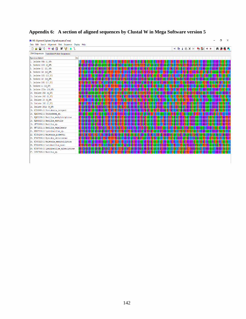
142

Appendix 6: A section of aligned sequences by Clustal W in Mega Software version 5

143

Appendix 7: Definition of terms

Anaerobic digestion It is the degradation of organic materials by microorganisms in the

absence of oxygen to CO2 and CH4.

Biochemical techniques Refers to a set of methods, assays and procedures to analyse the

substances found in living organisms and the chemical reactions

underlying life processes

Biodegradability It is the ability of materials to be capable of being disintegration by

bacteria, fungi, or other biological means.

BOD5 It is the amount of dissolved oxygen needed by aerobic biological

organisms to break down organic material present in a given water

sample at certain temperature over a five day period.

COD Is a measure of the capacity of water to consume oxygen during

the decomposition of organic matter and the oxidation of inorganic

chemicals such as Ammonia and nitrite.

Deoxyribonucleic acid (DNA) A self-replicating material present in nearly all living

organisms as the main constituent of chromosomes. It is the

carrier of genetic information.

DNA Sequencing Is the process of determining the sequences of nucleotide

bases (As, Ts, Cs and Gs)

144

Environment The surroundings or conditions in which a person, animal, or a

plant lives or operates.

Methanogens Microorganisms that produce methane as a metabolic byproduct in

anioxic conditions.

Molecular techniques Methods involving manipulation of DNA, RNA, protein, and lipids

Morphological techniques Analysis of the organisms with respect to the form, structure, and

their specific features.

Phylogenetic analysis Is the means of inferring or estimating relationships. The

evolutionary history inferred from phylogenetic analysis is usually

depicted as branching, tree like diagrams that represent an

estimated pedigree of the inherited relationships among molecules,

organisms or both.

Polymerase Chain Reaction (PCR) Is a method of oligonucleotide primer directed enzymatic

amplification of a specific DNA sequence of interest. It

amplifies a single copy or a few copies of a piece of DNA

across several orders of magnitude, generating thousands to

millions of copies of a particular DNA sequence.

Primers Is a strand of DNA bases that enables DNA to be replicated. They

are used primarily in Polymerase Chain Reaction and each primer

is single stranded DNA and is designed to match a specific piece of

template DNA. The specificity arises from the fact that each DNA

145

base can only pair with one other DNA base that is adenine (A)

pairs only with thymine (T) in DNA and uracil (U) in RNA, and

guanine (G) pairs only with cytosine (C). In order for copies to be

made, the primer must bind to the right piece of DNA and the

bases must match. If the matching occurs, then DNA polymerase

(the enzyme that copies the DNA) can bind and amplify the DNA.

If the primer does not match the DNA sequence, then the DNA

polymerase cannot bind and no copies will be made.