optimization. applications to image processing - sitio...
TRANSCRIPT

Optimization. Applications to image processing
Mila NIKOLOVA
CMLA (CNRS-UMR 8536)–ENS de Cachan, 61 av. du President Wilson, 94235 Cachan Cedex, [email protected]
http://www.cmla.ens-cachan.fr/∼nikolova/
Textbook : http://www.cmla.ens-cachan.fr/∼nikolova/Optim-MVD12.pdf
MONTEVIDEO, April 2012

1
Contents
. . . . . . . . . . . . . . . . . . . . . . . . . . . . . . . . . . . . . . . . . . . . . . . . . . . 1
1 Generalities 5
1.1 Optimization problems . . . . . . . . . . . . . . . . . . . . . . . . . . . . . . . . . . . 61.2 Analysis of the optimization problem . . . . . . . . . . . . . . . . . . . . . . . . . . . 10
1.2.1 Remainders . . . . . . . . . . . . . . . . . . . . . . . . . . . . . . . . . . . . . 101.2.2 Existence, uniqueness of the solution . . . . . . . . . . . . . . . . . . . . . . . 111.2.3 Equivalent optimization problems . . . . . . . . . . . . . . . . . . . . . . . . . 12
1.3 Optimization algorithms . . . . . . . . . . . . . . . . . . . . . . . . . . . . . . . . . . 171.3.1 Iterative minimization methods . . . . . . . . . . . . . . . . . . . . . . . . . . 171.3.2 Local convergence rate . . . . . . . . . . . . . . . . . . . . . . . . . . . . . . . 18
2 Unconstrained differentiable problems 21
2.1 Preliminaries (regularity of F ) . . . . . . . . . . . . . . . . . . . . . . . . . . . . . . . 212.2 One coordinate at a time (Gauss-Seidel) . . . . . . . . . . . . . . . . . . . . . . . . . 222.3 First-order (Gradient) methods . . . . . . . . . . . . . . . . . . . . . . . . . . . . . . 22
2.3.1 The steepest descent method . . . . . . . . . . . . . . . . . . . . . . . . . . . 232.3.2 Gradient with variable step-size . . . . . . . . . . . . . . . . . . . . . . . . . . 26
2.4 Line search . . . . . . . . . . . . . . . . . . . . . . . . . . . . . . . . . . . . . . . . . 272.4.1 Introduction . . . . . . . . . . . . . . . . . . . . . . . . . . . . . . . . . . . . . 272.4.2 Schematic algorithm for line-search . . . . . . . . . . . . . . . . . . . . . . . . 282.4.3 Modern line-search methods . . . . . . . . . . . . . . . . . . . . . . . . . . . . 29
2.5 Second-order methods . . . . . . . . . . . . . . . . . . . . . . . . . . . . . . . . . . . 322.5.1 Newton’s method . . . . . . . . . . . . . . . . . . . . . . . . . . . . . . . . . . 322.5.2 General quasi-Newton Methods . . . . . . . . . . . . . . . . . . . . . . . . . . 342.5.3 Generalized Weiszfeld’s method (1937) . . . . . . . . . . . . . . . . . . . . . . 362.5.4 Half-quadratic regularization . . . . . . . . . . . . . . . . . . . . . . . . . . . . 372.5.5 Standard quasi-Newton methods . . . . . . . . . . . . . . . . . . . . . . . . . 40
2.6 Conjugate gradient method (CG) . . . . . . . . . . . . . . . . . . . . . . . . . . . . . 422.6.1 Quadratic strongly convex functionals (Linear CG) . . . . . . . . . . . . . . . 422.6.2 Non-quadratic Functionals (non-linear CG) . . . . . . . . . . . . . . . . . . . . 432.6.3 Condition number and preconditioning . . . . . . . . . . . . . . . . . . . . . . 46
3 Constrained optimization 49
3.1 Preliminaries . . . . . . . . . . . . . . . . . . . . . . . . . . . . . . . . . . . . . . . . 493.2 Optimality conditions . . . . . . . . . . . . . . . . . . . . . . . . . . . . . . . . . . . . 49
3.2.1 Projection theorem . . . . . . . . . . . . . . . . . . . . . . . . . . . . . . . . . 503.3 General methods . . . . . . . . . . . . . . . . . . . . . . . . . . . . . . . . . . . . . . 51
3.3.1 Gauss-Seidel under Hyper-cube constraint . . . . . . . . . . . . . . . . . . . . 513.3.2 Gradient descent with projection and varying step-size . . . . . . . . . . . . . 513.3.3 Penalty . . . . . . . . . . . . . . . . . . . . . . . . . . . . . . . . . . . . . . . 54
3.4 Equality constraints . . . . . . . . . . . . . . . . . . . . . . . . . . . . . . . . . . . . . 563.4.1 Lagrange multipliers . . . . . . . . . . . . . . . . . . . . . . . . . . . . . . . . 56
CONTENTS 3
3.4.2 Application to linear systems . . . . . . . . . . . . . . . . . . . . . . . . . . . 583.5 Inequality constraints . . . . . . . . . . . . . . . . . . . . . . . . . . . . . . . . . . . . 60
3.5.1 Abstract optimality conditions . . . . . . . . . . . . . . . . . . . . . . . . . . . 603.5.2 Farkas-Minkowski (F-M) theorem . . . . . . . . . . . . . . . . . . . . . . . . . 613.5.3 Constraint qualification . . . . . . . . . . . . . . . . . . . . . . . . . . . . . . . 633.5.4 Kuhn & Tucker Relations . . . . . . . . . . . . . . . . . . . . . . . . . . . . . 64
3.6 Convex inequality constraint problems . . . . . . . . . . . . . . . . . . . . . . . . . . 653.6.1 Adaptation of previous results . . . . . . . . . . . . . . . . . . . . . . . . . . . 653.6.2 Duality . . . . . . . . . . . . . . . . . . . . . . . . . . . . . . . . . . . . . . . 673.6.3 Uzawa’s Method . . . . . . . . . . . . . . . . . . . . . . . . . . . . . . . . . . 72
3.7 Unifying framework and second-order conditions . . . . . . . . . . . . . . . . . . . . . 743.7.1 Karush-Kuhn-Tucker Conditions (1st order) . . . . . . . . . . . . . . . . . . . 743.7.2 Second order conditions . . . . . . . . . . . . . . . . . . . . . . . . . . . . . . 743.7.3 Standard forms (QP, LP) . . . . . . . . . . . . . . . . . . . . . . . . . . . . . 753.7.4 Interior point methods . . . . . . . . . . . . . . . . . . . . . . . . . . . . . . . 75
3.8 Nesterov’s approach . . . . . . . . . . . . . . . . . . . . . . . . . . . . . . . . . . . . . 76
4 Non differentiable problems 784.1 Specificities . . . . . . . . . . . . . . . . . . . . . . . . . . . . . . . . . . . . . . . . . 78
4.1.1 Examples . . . . . . . . . . . . . . . . . . . . . . . . . . . . . . . . . . . . . . 784.1.2 Kinks . . . . . . . . . . . . . . . . . . . . . . . . . . . . . . . . . . . . . . . . 79
4.2 Basic notions . . . . . . . . . . . . . . . . . . . . . . . . . . . . . . . . . . . . . . . . 804.2.1 Preliminaries . . . . . . . . . . . . . . . . . . . . . . . . . . . . . . . . . . . . 804.2.2 Directional derivatives . . . . . . . . . . . . . . . . . . . . . . . . . . . . . . . 814.2.3 Subdifferentials . . . . . . . . . . . . . . . . . . . . . . . . . . . . . . . . . . . 83
4.3 Optimality conditions . . . . . . . . . . . . . . . . . . . . . . . . . . . . . . . . . . . . 874.3.1 Unconstrained minimization problems . . . . . . . . . . . . . . . . . . . . . . . 874.3.2 General constrained minimization problems . . . . . . . . . . . . . . . . . . . 884.3.3 Minimality conditions under explicit constraints . . . . . . . . . . . . . . . . . 89
4.4 Minimization methods . . . . . . . . . . . . . . . . . . . . . . . . . . . . . . . . . . . 904.4.1 Subgradient methods . . . . . . . . . . . . . . . . . . . . . . . . . . . . . . . . 914.4.2 Some algorithms specially adapted to the shape of F . . . . . . . . . . . . . . 934.4.3 Variable-splitting combined with penalty techniques . . . . . . . . . . . . . . . 96
4.5 Splitting methods . . . . . . . . . . . . . . . . . . . . . . . . . . . . . . . . . . . . . . 984.5.1 Moreau’s decomposition and proximal calculus . . . . . . . . . . . . . . . . . . 994.5.2 Forward-Backward (FB) splitting . . . . . . . . . . . . . . . . . . . . . . . . . 1024.5.3 Douglas-Rachford splitting . . . . . . . . . . . . . . . . . . . . . . . . . . . . . 103
5 Appendix 106
Objectives: obtain a good knowledge of the most important optimization methods, provide tools to
help reading the literature, conceive and analyze new methods. At the implementation stage, numerical
methods are always on Rn.
Main References: [7, 14, 26, 44, 45, 46, 53, 69, 70, 72]
For remainders check Connexions: http://cnx.org/
CONTENTS 4
Notations and abbreviations
• Abbreviations:
– n.v.s.—normed vector space (V ).
– l.s.c.—lower semi-continuous (for a function).
– w.r.t.—with respect to
– resp.—respectively
• dim(.)—dimension.
• 〈. , .〉 inner product (≡ scalar product) on a n.v.s. V .
• �a� denotes the integer part of a ∈ R.
• O is an open subset (arbitrary).
• O(U) denotes an open subset of V containing U ⊂ V .
• int(U) stands for the interior of U .
• B(u, r) is the open ball centered at u with radius r. The relevant closed ball is B(u, r).
• N is the set of non negative integers.
• Rq+ = {v ∈ R
q : v[i] ≥ 0, 1 ≤ i ≤ q} for any positive integer q.
• R = R ∪ {+∞}.• (ei)
ni=1 is the canonical basis of Rn.
• For an n× n matrix B:
– BT is its transpose and BH its conjugate transpose.
– λi(B)—an eigenvalue of B.
– λmin(B) (resp. λmax(B))—the minimal (resp. the maximal) eigenvalue of B.
– Remind: the spectral radius of B isdef= max
1≤i≤n
∣∣λi(B)∣∣.
– B � 0—B is positive definite, B � 0—B is positive semi-definite.
• Id is the identity operator.
• diag(b[1], · · · , b[n]) is an n× n diagonal matrix whose diagonal entries are b[i], 1 ≤ i ≤ n.
• For f : V1 × V2 × · · ·Vm → Y where Vj, j ∈ {1, 2, · · · , m} and Y are n.v.s., Djf(u1, · · · , um)is the differential of f at u = (u1, · · · , um) with respect to uj.
• L(V ; Y ), for V and Y n.v.s., is the set of all linear continuous applications from V to Y .
• For A ∈ L(V ; Y ), its adjoint is A∗.
• Isom(V ; Y ) ⊂ L(V ; Y ) are all bijective applications that have a continuous inverse application.
• o-function—satisfies limt→∞ o(t)/t = 0
• O-function—satisfies limt→∞O(t)/t = K where K is a constant.
Chapter 1
Generalities
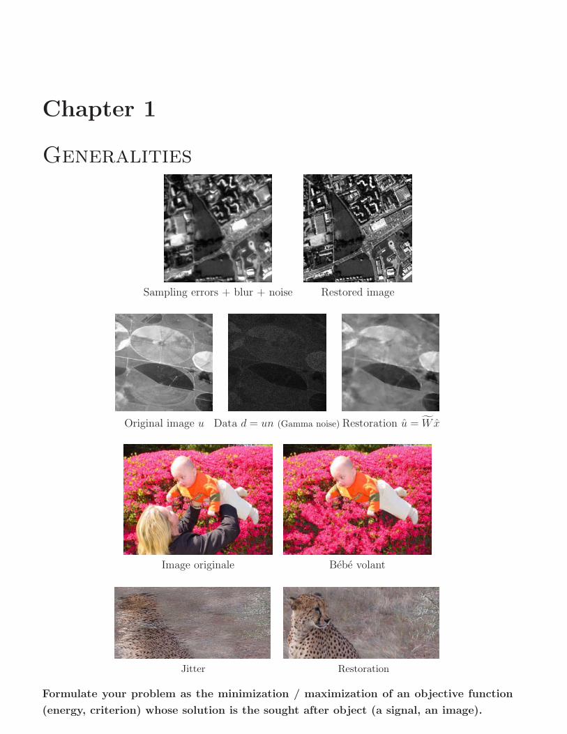
Sampling errors + blur + noise Restored image
Original image u Data d = un (Gamma noise) Restoration u = W x
Image originale Bebe volant
Jitter Restoration
Formulate your problem as the minimization / maximization of an objective function
(energy, criterion) whose solution is the sought after object (a signal, an image).
CHAPTER 1. GENERALITIES 6
1.1 Optimization problems
General Form : find a solution u ∈ V such that
(P ) u ∈ U and F (u) = infu∈U
F (u)
= − supu∈U
(− F (u))• F : V → R functional (objective function, criterion, energy) to minimize.
• V—real Hilbert space, if not explicitly specified.
• U ⊂ V constraint set, supposed nonempty and closed often convex.
Important cases:
equality constraints U = {u ∈ V : gi(u) = 0, i = 1, . . . , p}, p < n (1.1)
inequality constraints U = {u ∈ V : hi(u) ≤ 0, i = 1, . . . , q}, q ∈ N (1.2)
Minimizer u and minimum F (u).
Relative (local) minimum (resp. minimizer) and minimum global minimum (resp. minimizer).
Standard Form for quadratic functional:
F (u) =1
2B(u, u)− c(u), for B ∈ L(V × V ;R) and c ∈ L(V ;R), (1.3)
where B is bilinear and symmetric (i.e. B(u, v) = B(v, u), ∀u, v ∈ V ).
If V is equipped with an inner product 〈., .〉, we can write down (Riesz’s representation theorem)
F (u) =1
2〈Bu, u〉 − 〈c, u〉 (1.4)
If V = Rn in (1.4), B ∈ R
n×n is a symmetric matrix (i.e. B = BT ) and c ∈ Rn.
CHAPTER 1. GENERALITIES 7
Regularized objective functional on Rn
F (u) = Ψ(u) + βΦ(u) (1.5)
Φ(u) =∑i
ϕ(‖Diu‖) (1.6)
Diu—discrete approximation of the gradient or the Laplacian of the image or signal at i, or finite
differences, ‖.‖ is usually the �2 norm1, β > 0 parameter and ϕ : R+ → R+ increasing function, e.g.
ϕ(t) = tα, 1 ≤ α ≤ 2, ϕ(t) =√t2 + α, ϕ(t) = min{t2, α}, ϕ(t) = αt/(1 + αt), α > 0.
Ψ data-fitting term for data v ∈ Rm, usually A ∈ R
m×n and
Ψ(u) = ‖Au− v‖22, (1.7)
in some cases Ψ(u) = ‖Au− v‖1 or another function.
E.g. an image u of size p× q — rearranged into a n-length vector, n = pq:⎡⎢⎢⎢⎢⎢⎢⎢⎢⎢⎣
u[1] u[p+ 1] · · · · · · u[(q − 1)p+ 1]u[2] u[p+ 2] · · · · · · u[(q − 1)p+ 2]
· · ·...
... · · · u[i− 1] · · ·...
... · · · u[i− p] u[i] · · ·· · ·
u[p] u[2p] · · · · · · u[n]
⎤⎥⎥⎥⎥⎥⎥⎥⎥⎥⎦Often
‖Diu‖ =((u[i]− u[i−m])2 + (u[i]− u[i− 1])2
)1/2
(1.8)
or
‖Dku‖ =∣∣∣u[i]− u[i−m]
∣∣∣ and ‖Dk+1u‖ =∣∣∣u[i]− u[i− 1]
∣∣∣. (1.9)
If u is an one-dimensional signal, (1.8) and (1.9) amount to
‖Diu‖ =∣∣∣u[i]− u[i− 1]
∣∣∣, i = 2, · · · , n.
Di can also be any other linear mapping. If
Di = eTi , ∀i ∈ {1, · · · , n},
then
Φ(u) =∑i
ϕ( |u[i]| )
1For any p ∈ [1,+∞[, the �p norm of a vector v is defined by ‖v‖p =
(∑i
v[i]p
) 1p
and for p = +∞,
‖v‖∞ = maxi
∣∣v[i]∣∣.

CHAPTER 1. GENERALITIES 8
Illustration on the role of Φ
F (u) = ‖a ∗ u− v‖22 + β∑i
ϕ(‖Diu‖)
Original image Data v No Regularization
v = a � u+ n a—blurn—Normal noise SNR=20 dB β = 0 in (1.5)
ϕ(t) = tα ϕ(t) = t
Row 54 Row 54
Row 90 Row 90
ϕ(t) = αt2/(1 + αt2) ϕ(t) = αt/(1 + αt)
Row 54 Row 54
Row 90 Row 90
ϕ(t) = min{αt2, 1} ϕ(t) = 1− 1l(t=0)
Row 54 Row 54
Row 90 Row 90
Illustration on the role of Ψ
F (u) = ‖u− v‖22 + β‖Du‖1 F (u) = ‖u− v‖1 + β‖Du‖22 F (u) = ‖u− v‖22 + β‖Du‖22(a) Stair-casing (b) Exact data-fit (c)
D is a first-order difference operator, i.e. Diu = u[i]− u[i+ 1], 1 ≤ i ≤ p− 1. Data (- - -), Restored
signal (—). Constant pieces in (a) are emphasized using “∗” while data samples that are equal to
the relevant samples of the minimizer in (b) are emphasized using “◦”.
Table of Contents

CHAPTER 1. GENERALITIES 9
1. Generalities
2. Unconstrained differentiable problems
3. Constrained optimization
4. Non differentiable problems

CHAPTER 1. GENERALITIES 10
1.2 Analysis of the optimization problem
1.2.1 Remainders
Definition 1 Let F : V → ]−∞,+∞] where V is a real topological space.
- The domain of F is the set domF = {u ∈ V | F (u) < +∞}.
- The epigraph of F is the set epiF = {(u, λ) ∈ V × R | F (u) ≤ λ}.
Definition 2 A function F on a real n.v.s. V is proper if F : V → ] − ∞,+∞] and if it is not
identically equal to +∞.
Definition 3 F : V → R is coercive if lim‖u‖→∞
F (u) = +∞.
Definition 4 F : V → ]−∞,+∞] for V a real topological space
is lower semi-continuous (l.s.c.) if
∀λ ∈ R the set{u ∈ V | F (u) ≤ λ
}is is closed in V .
F is l.s.c.
If F is l.s.c., then −F is upper semi-continuous.
If F is continuous, then it is l.s.c. and upper semi-continuous.
Definition 5 (Convex subset) Let V be any real vector space. A subset U ⊂ V is convex if ∀u, v ∈ Uand θ ∈]0, 1[, we have θu+ (1− θ)v ∈ U .
u
v
u
v
U nonconvex U non strictly convex U strictly convex
Remind that F can be convex but not coercive.
Definition 6 (Convex function) Let V be any real vector space. A proper function F : U ⊂ V → R is
convex if ∀u, v ∈ U and θ ∈]0, 1[
F (θu+ (1− θ)v) ≤ θF (u) + (1− θ)F (v)
F is strictly convex when the inequality is strict whenever u �= v.
Property 1 Important properties [15, p. 8]:
- F is l.s.c. if and only if ∀u ∈ V and ∀ε > 0 there is a neighborhood O of u such that
F (v) ≥ F (u)− ε, ∀v ∈ O .
- If F is l.s.c.2 and uk → u as k →∞
lim infk→∞
F (uk) ≥ F (u).
2If F is upper semi-continuous and uk → u as k →∞ then lim supk→∞ F (uk) ≤ F (u).
CHAPTER 1. GENERALITIES 11
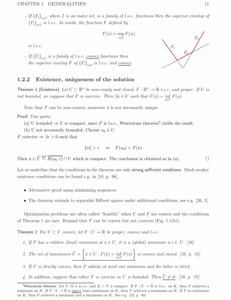
- If(Fi
)i∈I , where I is an index set, is a family of l.s.c. functions then the superior envelop of(
Fi
)i∈I is l.s.c. In words, the function F defined by
F (u) = supi∈I
Fi(u)
is l.s.c.
- If(Fi
)i∈I is a family of l.s.c. convex functions then
the superior envelop F of(Fi
)i∈I is l.s.c. and convex.
F1
F2
F3
1.2.2 Existence, uniqueness of the solution
Theorem 1 (Existence) Let U ⊂ Rn be non-empty and closed, F : Rn → R l.s.c. and proper. If U is
not bounded, we suppose that F is coercive. Then ∃u ∈ U such that F (u) = infu∈U
F (u).
Note that F can be non-convex; moreover u is not necessarily unique.
Proof. Two parts:
(a) U bounded ⇒ U is compact, since F is l.s.c., Weierstrass theorem3 yields the result.
(b) U not necessarily bounded. Choose u0 ∈ U .F coercive ⇒ ∃r > 0 such that
‖u‖ > r ⇒ F (u0) < F (u)
Then u ∈ U def= B(u0, r) ∩ U which is compact. The conclusion is obtained as in (a). �
Let us underline that the conditions in the theorem are only strong sufficient conditions. Much weaker
existence conditions can be found e.g. in [10, p. 96].
• Alternative proof using minimizing sequences.
• The theorem extends to separable Hilbert spaces under additional conditions, see e.g. [26, 5].
Optimization problems are often called “feasible” when U and F are convex and the conditions
of Theorem 1 are met. Remind that F can be convex but not coercive (Fig. 1.1(b)).
Theorem 2 For U ⊂ V convex, let F : U → R be proper, convex and l.s.c.
1. If F has a relative (local) minimum at u ∈ U , it is a (global) minimum w.r.t. U . [26]
2. The set of minimizers U =
{u ∈ U : F (u) = inf
u∈UF (u)
}is convex and closed. [38, p. 35]
3. If F is strictly convex, then F admits at most one minimum and the latter is strict.
4. In addition, suppose that either F is coercive or U is bounded. Then U �= ∅. [38, p. 35]
3Weierstrass theorem: Let V be a n.v.s. and K ⊂ V a compact. If F : V → R is l.s.c. on K, then F achieves aminimum on K. If F : V → R is upper semi continuous on K, then F achieves a maximum on K. If F is continuouson K, then F achieves a minimum and a maximum on K. See e.g. [52, p. 40]

CHAPTER 1. GENERALITIES 12
−1.72 6.86
0.21
2.94
two local
minimizers
u0
F (u)
u
No minimizer
1 8
F (u)
u
U = [1, 8]
(a)F nonconvex (b)F convex non coercive U = R (c)F convex non coercive U compact
1 8
U = [1, 8]
F (u)
u−1.89 1.89
0
F (u)
uminimizers3.51
0.38
F (u)
u
(d)F strongly convex, U compact (e)F non strictly convex (f)F strongly convex on R
Figure 1.1: Illustration of Definition 6 and Theorem 2. Minimizers are depicted with a thick point.
1.2.3 Equivalent optimization problems
Given an optimization problem defined by F : V → R and U ⊂ V ,
(P ) find u such that F (u) = infu∈U
F (u) ⇔ find u = arg infu∈U
F (u)
there are many different optimization problems that are in some way equivalent to (P ). For instance
• w = argminXF(w) where F : W → R, X ⊂W and there is f : W → V such that u = f(w);
• (u, b) = argminu∈U
maxb∈XF(u, b) where F : V ×W → R, U ⊂ V , X ⊂ W and u solves (P );
Some of these equivalent optimization problems are easier to solve than the original (P ). We shall
see such reformulations in what follows. The way enabling to recover them is in general an open
question. In many cases, such a reformulation (found by intuition and proven mathematically) is
valid only for a particular problem (P ).
There are several duality principles in optimization theory relating a problem expressed in terms
of vectors in an n.v.s. V to a problem expressed in terms of hyperplanes in the n.v.s.
Definition 7 A hyperplane (affine) is a set of the form
[h = α]def= {w ∈ V | 〈h, w〉 = α}
where h : V → R is a linear nonzero functional and α ∈ R is a constant.
A milestone is the Hahn-Banach theorem, stated below in its geometric form [15, 52].
Definition 8 Let U ⊂ V and K ⊂ V . The hyperplane [h = α] separates K and U
- nonstrictly if 〈h, w〉 � α, ∀w ∈ U and 〈h, w〉 � α, ∀w ∈ K;
CHAPTER 1. GENERALITIES 13
- strictly if there exists ε > 0 such that 〈h, w〉 − ε � α, ∀w ∈ U and 〈h, w〉+ ε � α, ∀w ∈ K.
Theorem 3 (Hahn-Banach theorem, geometric form) Let U ⊂ V and K ⊂ V be convex, nonempty and
disjoint sets.
(i) If U is open, there is a closed hyperplane4 [h = α] that separates K and U nonstrictly;
(ii) If U is closed and K is compact5, then there exists a closed hyperplane [h = α] that separates
K and U in a strict way.
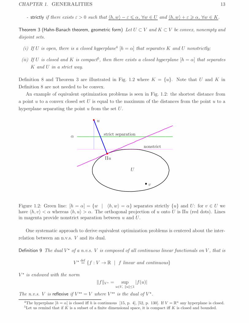
Definition 8 and Theorem 3 are illustrated in Fig. 1.2 where K = {u}. Note that U and K in
Definition 8 are not needed to be convex.
An example of equivalent optimization problems is seen in Fig. 1.2: the shortest distance from
a point u to a convex closed set U is equal to the maximum of the distances from the point u to a
hyperplane separating the point u from the set U .
strict separation
nonstrict
U
u
Πu
v
α
Figure 1.2: Green line: [h = α] = {w | 〈h, w〉 = α} separates strictly {u} and U : for v ∈ U wehave 〈h, v〉 < α whereas 〈h, u〉 > α. The orthogonal projection of u onto U is Πu (red dots). Linesin magenta provide nonstrict separation between u and U .
One systematic approach to derive equivalent optimization problems is centered about the inter-
relation between an n.v.s. V and its dual.
Definition 9 The dual V � of a n.v.s. V is composed of all continuous linear functionals on V , that is
V � def= {f : V → R | f linear and continuous}
V � is endowed with the norm
‖f‖V � = supu∈V, ‖u‖≤1
|f(u)|
The n.v.s. V is reflexive if V �� = V where V �� is the dual of V �.
4The hyperplane [h = α] is closed iff h is continuous [15, p. 4], [52, p. 130]. If V = Rn any hyperplane is closed.
5Let us remind that if K is a subset of a finite dimensional space, it is compact iff K is closed and bounded.

CHAPTER 1. GENERALITIES 14
If V = Rn then V � = R
n (see e.g. [52, p. 107]). The dual of the Hilbert space6 L2 (resp. �2) is
yet again L2 (resp. �2)—see e.g. [52, pp. 107-109]. Clearly, all these spaces are reflexive as well.
Definition 10 Let F defined on a real n.v.s. V be proper. The function F � : V � → R given by
F �(v)def= sup
u∈V
{ 〈u, v〉 − F (u)} (1.10)
is called the convex conjugate or the polar function of F .
The Fenchel-Young inequality:
u ∈ V, v ∈ V � ⇒ 〈u, v〉 ≤ F (u) + F �(v) (1.11)
0
epiFepiF
FF
uu
F (u�)F (u�)
−F �(v)−F �(v)
Figure 1.3: The convex conjugate at v determines an hyperplane that separates nonstrictly epiFand its complement in R
n.
The application v �→ 〈u, v〉 − F (u) is convex and continuous, hence l.s.c., for any fixed u ∈ V .
According to Property 1, F � is convex and l.s.c. (as being a superior convex envelop).
Example 1 Let f(u) =1
α|u|α where u ∈ R and α ∈]1,+∞[.
f �(v) = supu∈R
(uv − 1
α|u|α
)The term between the parentheses obviously has a unique global maximizer u. The latter meets
v = |u|α−1sign(u) hence sign(u) = sign(v). Then
u = |v| 1α−1 sign(v)
Set α� = αα−1
which is the same as1
α+
1
α�= 1 (1.12)
We have α� ∈]1,+∞[ and
f �(v) = |v| 1α−1 sign(v)v − 1
α|v| α
α−1 = |v| αα−1
(1− 1
α
)=
1
α�|v|α�
(1.13)
6Remind that Rn is a Hilbert space as well.
CHAPTER 1. GENERALITIES 15
Extension: For u ∈ Rn and α ∈]1,+∞[, let
F (u) =1
α‖u‖αα
Then v ∈ Rn and
F �(v) = supu∈Rn
(〈u, v〉 − 1
α‖u‖αα
)= sup
u∈Rn
n∑i=1
(u[i]v[i]− 1
α|u[i]|α
)=
n∑i=1
supu∈Rn
(u[i]v[i]− 1
α|u[i]|α
)=
n∑i=1
f �(v[i]) =
n∑i=1
1
α�|v[i]|α�
=1
α�‖v‖α�
α�
where f � is given by (1.13) and α� meets (1.13)
We can repeat the process in (1.10), thereby leading to the bi-conjugate F �� : V → R:
F ��(u)def= sup
v∈V �
{ 〈u, v〉 − F �(v)}
One can note that F ��(u) ≤ F (u), ∀u ∈ V .
Theorem 4 (Fenchel-Moreau) Let F , defined on a real n.v.s. V , be proper and convex. Then
F �� = F
For the proof, see [15, p. 10] or [73, 38].
The theorem below is an important tool to equivalently reformulate optimization problems.
Theorem 5 (Fenchel-Rockafellar) Let Φ and Ψ be convex on V . Assume that there exists u0 such that
Φ(u0) < +∞, Ψ(u0) < +∞ and Φ is continuous at u0. Then
infu∈V
(Φ(u) + Ψ(u)
)= max
v∈V �(−Φ�(−v)−Ψ�(v)
)
The proof can be found in [15, p. 11] or in [52, p. 201] (where the assumptions on Φ and Ψ are
slightly different).
Example 2 V is a real reflexive n.v.s. Let U ⊂ V and K ⊂ V � be convex compact nonempty subsets.
Ψ(u)def= sup
v∈K〈v, u〉 = max
v∈K〈v, u〉 ≤ max
v∈K‖v‖ ‖u‖ (1.14)
where Schwarz inequality was used. Note that we can replace sup with max in (1.14) because K is
compact and v �→ 〈v, u〉 is continuous (Weierstrass theorem). Clearly maxv∈K‖v‖ is finite and Ψ is
continuous and convex.

CHAPTER 1. GENERALITIES 16
• Let w ∈ V � \K. The set {w} being compact, Hahn-Banach theorem 3 tells us that there exists
h ∈ V �� = V enabling us to separate strictly {w} and K ⊂ V �, that is
〈v, h〉 < 〈w, h〉 , ∀v ∈ K
and the constant cdef= inf
v∈K( 〈w, h〉 − 〈v, h〉 ) meets c > 0. Then
〈w, h〉 − 〈v, h〉 ≥ c > 0, ∀ v ∈ K ⇔ 〈w, h〉 − supv∈K〈v, h〉 ≥ c > 0
Using that αh ∈ V for any α > 0, we have
Ψ�(w) = supu∈V
( 〈w, u〉 −Ψ(u)) ≥ sup
α>0
( 〈w, αh〉 −Ψ(αh))= sup
α>0
(α 〈w, h〉 − sup
v∈K〈v, αh〉 )
= supα>0
α( 〈w, h〉 − sup
v∈K〈v, h〉 ) ≥ c sup
α>0α = +∞. (1.15)
• Let now w ∈ K ⊂ V �. Then 〈w, u〉 −maxv∈K 〈v, u〉 ≤ 0, ∀u ∈ V , hence
Ψ�(w) = supu∈V
( 〈w, u〉 −Ψ(u))= sup
u∈V
( 〈w, u〉 −maxv∈K〈v, u〉 ) = 0 (1.16)
where the upper bound 0 is always reached for u = 0.
• Combining (1.15) and (1.16) shows that the convex conjugate of Ψ reads
Ψ�(v) =
{+∞ if v �∈ K0 if v ∈ K
• Set
Φ(u) =
{+∞ if u �∈ U0 if u ∈ U
By the definition of Ψ in (1.14) and the one of Φ, the Fenchel-Rockafellar Theorem 5 yields
minu∈U
(maxv∈K〈u, v〉 ) = min
u∈UΨ(u) = min
u∈V(Φ(u) + Ψ(u)
)= max
v∈V �
(− Φ�(−v)−Ψ�(v))
(1.17)
The maximum in the right side cannot be reached if v �∈ K because in this case −Ψ�(v) = −∞.
Hence maxv∈V �
(− Φ�(−v)−Ψ�(v))= max
v∈K(− Φ�(−v)). Furthermore
−Φ�(−v) = − supu∈U
(− 〈v, u〉 − Φ(u))= inf
u∈U( 〈v, u〉+ Φ(u)
)= inf
u∈U〈v, u〉 = min
u∈U〈v, u〉
It follows that
maxv∈V �
(−Ψ�(v)− Φ�(−v)) = maxv∈K
(minu∈U〈v, u〉 ) (1.18)
Combining (1.17) and (1.18) shows that minu∈U(maxv∈K 〈u, v〉
)= maxv∈K
(minu∈U 〈v, u〉
).
In Example 2 we have proven the fundamental Min-Max theorem used often in classical game
theory. The precise statement is given below.
Theorem 6 (Min-Max) Let V be a reflexive real n.v.s. Let U ⊂ V and K ⊂ V � be convex, compact
nonempty subsets. Then
minu∈U
maxv∈K〈u, v〉 = max
v∈Kminu∈U〈v, u〉

CHAPTER 1. GENERALITIES 17
1.3 Optimization algorithms
Usually the solution u is defined implicitly and cannot be computed in an explicit way, in one step.
1.3.1 Iterative minimization methods
Construct a sequence (uk)k∈N initialized by u0 converging to u—a solution of (P ):
uk+1 = G(uk), k = 0, 1, . . . , (1.19)
where G : V → U is called iterative scheme (often defined implicitly). The solution u can be
local (relative) if (P ) is nonconvex. The choice of u0 (= the initialization) can be crucial if (P ) is
nonconvex.
G is constructed using information on (P ), e.g. F (uk), ∇F (uk), gi(uk), hi(uk), ∇gi(uk) and
∇hi(uk) (or subgradients instead of ∇ for nonsmooth functions).
By (1.19), the iterates of G read
u1 = G(u0);
u2 = G(u1) = G ◦G(u0) def= G2(u0);
· · ·uk = G ◦ · · · ◦G︸ ︷︷ ︸ (u0)
def= Gk(u0) = G ◦Gk−1(u0)
k times
Key questions:
• Given an iterative method G, determine if there is convergence;
• If convergence, to what kind of accumulation point?
• Given two iterative methods G1 and G2 choose the faster one.
Definition 11 u is a fixed point for G if G(u) = u.
Let X be a metric space equipped with distance d.
Definition 12 G : X → X is a contraction if there exists γ ∈ (0, 1) such that
d(G(u1), G(u2)) ≤ γd(u1, u2), ∀u1, u2 ∈ X
⇒ G is Lipschitzian7 ⇒ uniformly continuous.
Theorem 7 (Fixed point theorem) Let X be complete and G : X → X a contraction.
Then G admits a unique fixed point, u = G(u). (see [77, p.141]).
Theorem 8 (Fixed point theorem-bis) Let X be complete and G : X → X be such that ∃k0 for which
Gk0 is a contraction. Then G admits a unique fixed point. (see [77, p.142]).
Note that in the latter case G is not necessarily a contraction.
7A function f : V → X is �-Lipschitz continuous if ∀(u, v) ∈ V × V , we have ‖f(u)− f(v)‖ ≤ � ‖f(u)− f(v)‖.
CHAPTER 1. GENERALITIES 18
1.3.2 Local convergence rate
In general, a nonlinear problem (P ) cannot be solved exactly in a finite number of iterations.
Goal: attach to G precise indicators of the asymptotic rate of convergence of uk towards u. Refs.
[70, 69, 26, 14]
Here V = Rn, ‖ · ‖ = ‖ · ‖2 and we simply assume that uk converges to u.
Q-convergence studies the quotient Qkdef=‖uk+1 − u‖‖uk − u‖ , k ∈ N.
Q = lim supk→∞
Qk
• If Q <∞ then ∀ε > 0 ∃k0 such that
‖uk+1 − u‖ ≤ (Q + ε)‖uk − u‖, ∀k ≥ k0.
≡ Bound on the error at iteration k+1 in terms of the error at iteration k. (Crucial if Q < 1.)
• 0 < Q < 1: Q-linear convergence;
• Q = 0: Q-superlinear convergence (called also superlinear convergence);
• In particular, Qk = O(‖uk − u‖2): Q-quadratic convergence.
• Compare how G1 and G2 converge towards the same u:
If Q(G1, u) < Q(G2, u) then G1 is faster than G2 in the sense of Q.
R-convergence studies the rate of the root Rkdef= ‖uk − u‖1/k, k ∈ N.
R = lim supk→∞
Rk
• 0 < R < 1: R-linear convergence; this means geometric or exponential convergence since
∀ε ∈ (0, 1−R) ∃k0 such that Rk ≤ (R + ε), ∀k ≥ k0 ⇐⇒ ‖uk − u‖ ≤ (R + ε)k
• R = 0: R-superlinear convergence.
• G1 is faster than G2 in the sense of R if R(G1, u) < R(G2, u)
Remark 1 Sublinear convergence if Qk → 1 or Rk → 1. Convergence is too slow, choose another G.
Theorem 9 Let ‖uk− u‖ ≤ vk where (vk)k∈N converges to 0 Q-superlinearly. Then (uk)k∈N converges
to u R-superlinearly.
Theorem 10 Let uk → u R-linearly. Then ∃ (vk)k∈N that tends to 0 Q-linearly such that ‖uk−u‖ ≤ vk.
Proofs of the last two theorems - see [14, p.15].
CHAPTER 1. GENERALITIES 19
Lemma 1 Let G : U ⊂ Rn → R
n, ‖.‖ be any norm on Rn, ∃B(u, δ) ⊂ U and ∃γ ∈ [0, 1) such that
‖G(u)− u‖ ≤ γ‖u− u‖, ∀u ∈ B(u, δ)
Then ∀u0 ∈ B(u, δ) the iterates given by (1.19) remain in B(u, δ) and converge to u.
Proof. Let u0 ∈ B(u, δ), then ‖u1 − u‖ = ‖G(u0)− u‖ ≤ γ‖u0 − u‖ < ‖u0 − u‖, hence u1 ∈ B(u, δ).
Using induction, uk ∈ B(u, δ) and ‖uk − u‖ ≤ γk‖u0 − u‖. Thus limk→∞ uk = u. �
Theorem 11 (Ostrowski) [70, p.300] Let G : U ⊂ Rn → R
n be differentiable at u ∈ int(U) and has
a fixed point G(u) = u ∈ U . If
σdef= max
1≤i≤n
∣∣λi(∇G(u))∣∣ < 1, (1.20)
then ∃O(u) such that ∀u0 ∈ O(u) we have uk ∈ O(u) and uk → u.
Proof. ∇G(u) is not necessarily symmetric and positive definite. Condition (1.20) says that
∀ε > 0 there is an induced matrix norm ‖.‖ on Rn×n such that8
‖∇G(u)‖ ≤ σ + ε. (1.21)
Let us choose ε such that
ε <1
2(1− σ).
The differentiability of G at u implies that ∃δ > 0 so that B(u, δ) ⊂ U and
‖G(u)−G(u)−∇G(u)(u− u)‖ ≤ ε‖u− u‖, ∀u ∈ B(u, δ) (1.22)
Using that G(u) = u, and combining (1.21) and (1.22), we get
‖G(u)− u‖ = ‖G(u)−G(u)−∇G(u)(u− u) +∇G(u)(u− u)‖≤ ‖G(u)−G(u)−∇G(u)(u− u)‖+ ‖∇G(u)‖ ‖u− u‖< (2ε+ σ)‖u− u‖ < ‖u− u‖, ∀u ∈ B(u, δ)
The conclusion follows from the observation that 2ε+ σ < 1 and Lemma 1. �
8Let B be an n× n real matrix. Its spectral radius is defined as its largest in absolute value eigenvalue,
σ(B)def= max
1≤i≤n
∣∣λi(B)∣∣.
Given a vector norm on Rn, say ‖.‖, the corresponding induced matrix norm on the space of all n× n matrices reads
‖B‖ def= sup{‖Bu‖ : u ∈ R
n, ‖u‖ ≤ 1}.Theorem 12 [26, p. 18]
(1) Let B be an n× n matrix and ‖ . ‖ any matrix norm. Then
σ(B) ≤‖ B ‖ .
(2) Given a matrix B and a number ε > 0, there exists at least one induced matrix norm ‖ . ‖ such that
‖ B ‖≤ σ(B) + ε.
CHAPTER 1. GENERALITIES 20
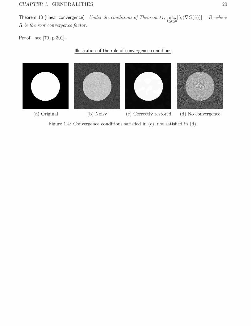
Theorem 13 (linear convergence) Under the conditions of Theorem 11, max1≤i≤n
|λi(∇G(u))| = R, where
R is the root convergence factor.
Proof—see [70, p.301].
Illustration of the role of convergence conditions
(a) Original (b) Noisy (c) Correctly restored (d) No convergence
Figure 1.4: Convergence conditions satisfied in (c), not satisfied in (d).
Chapter 2
Unconstrained differentiable problems
2.1 Preliminaries (regularity of F )
Remainders (see e.g. [78, 11, 26]):
1. For V and Y real n.v.s., f : V → Y if differentiable at u ∈ V if ∃Df(u) ∈ L(V, Y ) (linear
continuous application from V to Y ) such that
f(u+ v) = f(u) +Df(u)v + ‖v‖ε(v) where limv→0
ε(v) = 0.
2. If Y = R (i.e. f : V → R) and the norm on V is derived from an inner product 〈., .〉, thenL(V ;R) is identified to V (via a canonical isomorphism). Then ∇f(u) ∈ V—the gradient of
f at u is defined by
〈∇f(u), v〉 = Df(u)v, ∀v ∈ V.Note that if V = R
n we have Df(u) = (∇f(u))T .
3. Under the conditions given above in 2., if f is twice differentiable, we can identify the second
differential D2f and the Hessian ∇2f via D2f(u)(v, w) = 〈∇2f(u)v, w〉.
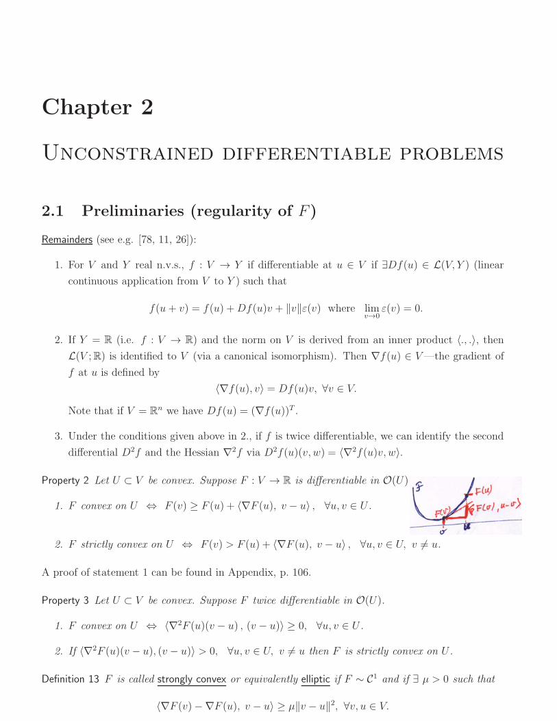
Property 2 Let U ⊂ V be convex. Suppose F : V → R is differentiable in O(U).
1. F convex on U ⇔ F (v) ≥ F (u) + 〈∇F (u), v − u〉 , ∀u, v ∈ U .
2. F strictly convex on U ⇔ F (v) > F (u) + 〈∇F (u), v − u〉 , ∀u, v ∈ U, v �= u.
A proof of statement 1 can be found in Appendix, p. 106.
Property 3 Let U ⊂ V be convex. Suppose F twice differentiable in O(U).
1. F convex on U ⇔ 〈∇2F (u)(v − u) , (v − u)〉 ≥ 0, ∀u, v ∈ U .
2. If 〈∇2F (u)(v − u), (v − u)〉 > 0, ∀u, v ∈ U, v �= u then F is strictly convex on U .
Definition 13 F is called strongly convex or equivalently elliptic if F ∼ C1 and if ∃ μ > 0 such that
〈∇F (v)−∇F (u), v − u〉 ≥ μ‖v − u‖2, ∀v, u ∈ V.
CHAPTER 2. UNCONSTRAINED DIFFERENTIABLE PROBLEMS 22
F in (1.4) is strongly convex if and only if B � 0.
Property 4 Suppose F : V → R is differentiable in V .
1. F : V → R strongly convex ⇒ F is strictly convex, coercive and
F (v)− F (u) ≥ 〈∇F (u), v − u〉+ μ
2‖v − u‖2, ∀v, u ∈ V .
2. Suppose F twice differentiable in V :
F strongly convex ⇔ 〈∇2F (u)v, v〉 ≥ μ‖v‖2, ∀v ∈ V .
Remark 2 If F : Rn → R is twice differentiable, then ∇2F (u) (known as the Hessian of F at u) is
an n× n symmetric matrix, ∀u ∈ Rn. Indeed,
(∇2F (u))[i, j] = ∂2F (u)
∂u[i]∂u[j]=(∇2F (u)
)[j, i].
2.2 One coordinate at a time (Gauss-Seidel)
We consider the minimization of a coercive proper convex function F : Rn → R.
For each k ∈ N, the algorithm involves n steps: for i = 1, . . . , n, uk+1[i] is updated according to
F (uk+1[1], . . . , uk+1[i− 1], uk+1[i], uk[i+ 1], . . . , uk[n])
= infρ∈R
F (uk+1[1], . . . , uk+1[i− 1], ρ, uk[i+ 1], . . . , uk[n])
Theorem 14 F is C1, strictly convex and coercive ⇒ (uk)k∈N converges to u. (see [44])
Remark 3 Differentiability is essential. E.g. apply the method to
F (u[1], u[2]) = u[1]2 + u[2]2 − 2(u[1] + u[2]
)+ 2
∣∣u[1]− u[2]∣∣ with u0 = (0, 0).
Note that infR2 F (u) = F (1, 1) = −2.
Remark 4 Extension for F (u) = ‖Au− v‖2 +∑λi|u[i]|, see [44].
2.3 First-order (Gradient) methods
They use F (u) and ∇F (u) and rely on F (uk − ρkdk) ≈ F (uk)− ρk 〈∇F (uk), dk〉. Different tasks:
• Choose a descent direction (−dk) - such that F (uk − ρdk) < F (uk) for ρ > 0 small enough;
• Line search : find ρk such that F (uk − ρkdk)− F (uk) < 0 is sufficiently negative.
• Stopping rule: introduce an error function which measures the quality of an approximate
solution u, e.g. choose a norm ‖.‖, τ > 0 (small enough) and test:
– Iterates: if ‖uk+1 − uk‖ ≤ τ , then stop ;
– Gradient: if ‖∇F (uk)‖ ≤ τ , then stop ;
– Objective: if F (uk)− F (uk+1) ≤ τ , then stop ;

CHAPTER 2. UNCONSTRAINED DIFFERENTIABLE PROBLEMS 23
or a combination of these.
Descent direction −dk for F at uk ⇔ F (uk − ρdk) < F (uk), ρ > 0 (small enough)
F differentiable:
〈∇F (uk), dk〉 > 0 ⇒ −dk is a descent direction for F at uk (2.1)
F convex and differentiable:
〈∇F (uk), dk〉 > 0 ⇔ −dk is a descent direction for F at uk (2.2)
F : R2 → R smooth strictly convex F : R2 → R smooth nonconvexone minimizer two minimizers
Proof. Using a first-order expansion,
F (uk − ρdk) = F (uk)− ρ 〈∇F (uk), dk〉+ ρ‖dk‖ ε(ρdk) (2.3)
where ε(ρdk)→ 0 as ρ→ 0 (2.4)
Then (2.3) can be rewritten as
F (uk)− F (uk − ρdk) = ρ(〈∇F (uk), dk〉 − ‖dk‖ ε(ρdk)
).
Consider that 〈∇F (uk), dk〉 > 0. By (2.4), there is ρ > 0 such that 〈∇F (uk), dk〉 > ‖dk‖ ε(ρdk),0 < ρ < ρ. Then −dk is a descent direction since F (uk)− F (uk − ρdk) > 0, 0 < ρ < ρ.
When F is convex, we know by Property 2-1 that F (uk − ρdk) ≥ F (uk) + 〈∇F (uk),−ρdk〉, i.e.
F (uk)− F (uk − ρdk) ≤ ρ 〈∇F (uk), dk〉 .
If 〈∇F (uk), dk〉 ≤ 0 then F (uk)− F (uk − ρdk) ≤ 0, hence −dk is not a descent direction. It follows
that for −dk to be a descent direction, it is necessary that 〈∇F (uk), dk〉 > 0. �
Note that some methods construct ρkdk in an automatic way.
2.3.1 The steepest descent method
Motivation : make F (uk)−F (uk+1) as large as possible. In (2.3) we have 〈∇F (uk), dk〉 ≤ ‖F (uk)‖ ‖dk‖(Schwarz inequality) where the equality is reached if dk ∝ ∇F (uk).
The steepest descent method = Gradient with optimal stepsize is defined by
F (uk − ρk∇F (uk)) = infρ∈R
F (uk − ρ∇F (uk)) (2.5)
uk+1 = uk − ρk∇F (uk), k ∈ N. (2.6)
CHAPTER 2. UNCONSTRAINED DIFFERENTIABLE PROBLEMS 24
Theorem 15 If F : Rn → R is strongly convex, (uk)k∈N given by (2.5)-(2.6) converges to the unique
minimizer u of F .
Proof. Suppose that ∇F (uk) �= 0 (otherwise u = uk). Proof in 5 steps.
(a) Denote
fk(ρ) = F(uk − ρ∇F (uk)
), ρ > 0.
fk is coercive, strictly convex, hence it admits a unique minimizer ρdef= ρ(uk) and the latter
solves the equation f ′k(ρ) = 0. Thus
f ′k(ρ) = −
⟨∇F (uk − ρ∇F (uk)) , ∇F (uk)⟩ = 0 (2.7)
Since
uk+1 = uk − ρ∇F (uk) ⇔ ∇F (uk) = 1
ρ(uk − uk+1) (2.8)
the left hand side of (2.8) inserted into (2.7) yields
〈∇F (uk+1),∇F (uk)〉 = 0, (2.9)
i.e. two consecutive directions are orthogonal, while the right hand side equation of (2.8) inserted
into (2.7) shows that
〈∇F (uk+1), uk − uk+1〉 = 0.
Using the last equation and the assumption that F is strongly convex,
F (uk)− F (uk+1) ≥ 〈∇F (uk+1), uk − uk+1〉+ μ
2‖uk − uk+1‖2 = μ
2‖uk − uk+1‖2 (2.10)
(b) Since(F (uk)
)k∈N is decreasing and bounded from below by F (u) we deduce that
(F (uk)
)k∈N
converges, hence
limk→∞
(F (uk)− F (uk+1)
)= 0
Inserting this result into (2.10) shows that 1
limk→∞‖uk − uk+1‖ = 0 (2.11)
(c) Using (2.9) allows us to write down
‖∇F (uk)‖2 = 〈∇F (uk),∇F (uk)〉 − 〈∇F (uk),∇F (uk+1)〉 = 〈∇F (uk),∇F (uk)−∇F (uk+1)〉
By Schwarz’s inequality,
‖∇F (uk)‖2 ≤ ‖∇F (uk)‖ ‖∇F (uk)−∇F (uk+1)‖
hence
‖∇F (uk)‖ ≤ ‖∇F (uk)−∇F (uk+1)‖ (2.12)
1Remind that (2.11) does not mean that the sequence (uk) converges!
Consider uk =∑k
i=01
k+1 . It is well known that (uk)k∈N diverges. Nevertheless, uk+1 − uk = 1k+2 → 0 as k →∞.

CHAPTER 2. UNCONSTRAINED DIFFERENTIABLE PROBLEMS 25
(d) The facts that(F (uk)
)k∈N is decreasing and that F is coercive implies that ∃ r > 0 such that
uk ∈ B(0, r), ∀k ∈ N. Since F ∼ C1, ∇F is uniformly continuous on the compact B(0, r). Using
(2.11), ∀ε > 0 there are η > 0 and k0 ∈ N such that
‖uk − uk+1‖ < η ⇒ ‖∇F (uk)−∇F (uk+1)‖ < ε, ∀k ≥ k0.
Consequently,
limk→∞‖∇F (uk)−∇F (uk+1)‖ = 0.
Combining this result with (2.12) shows that
limk→∞∇F (uk) = 0. (2.13)
(e) Using that F is strongly convex, that ∇F (u) = 0 and Schwarz’s inequality,
μ‖uk − u‖2 ≤ 〈∇F (uk)−∇F (u) , uk − u〉 = 〈∇F (uk) , uk − u〉 ≤ ‖∇F (uk)‖ ‖uk − u‖.Thus we have a bound on the error at iteration k
‖uk − u‖ ≤ 1
μ‖∇F (uk)‖ → 0 as k →∞
where the convergence result is due to (2.13). �
Remark 5 Note the role of the assumption that V = Rn is of finite dimension in this proof.
Quadratic strictly convex problem. Consider F : Rn → R of the form:
F (u) =1
2〈Bu, u〉 − 〈c, u〉 , B � 0, B = BT . (2.14)
Since B is symmetric and B � 0, hence F is strongly convex2.
∇F (u) = Bu− c (remind B = BT )
dk = ∇F (uk), k = 0, 1, · · ·f(ρ) = F
(uk − ρ∇F (uk)
)= F
(uk − ρ(Buk − c)
).
The steepest descent requires ρk such that f ′(ρk) = 0.
0 = f ′(ρk) = − ⟨∇F (uk − ρk∇F (uk)) , ∇F (uk)⟩= − ⟨
B(uk − ρk∇F (uk)
)− c , ∇F (uk)⟩= −〈(Buk − c)− ρkB∇F (uk) , ∇F (uk)〉= −〈∇F (uk)− ρkB∇F (uk) , ∇F (uk)〉= −‖∇F (uk)‖2 + ρk 〈B∇F (uk) , ∇F (uk)〉= −‖dk‖2 + ρk 〈Bdk , dk〉 ⇒ ρk =
‖dk‖2〈Bdk, dk〉
2Using that B � 0 and that B = BT , the lest eigenvalue of B, denoted by λmin, obeys λmin > 0. UsingDefinition 13,
〈∇F (v)−∇F (u), v − u〉 = (v − u)TB(v − u) ≥ λmin‖v − u‖22.
CHAPTER 2. UNCONSTRAINED DIFFERENTIABLE PROBLEMS 26
The full algorithm: for any k ∈ N, do
dk = Buk − cρk =
‖dk‖2〈Bdk, dk〉
uk+1 = uk − ρkdk
⇔ a method to solve a linear system Bu = c when B � 0 and BT = B.
Theorem 16 The statement of Theorem 15 holds true if F is C1, strictly convex and coercive.
Proof. (Sketch.) F (uk) is decreasing, bounded from below. Then ∃θ > 0 such that uk ∈B(0, θ), ∀k ∈ N, i.e. (uk)k∈N is bounded. Hence there exists a convergent subsequence
(ukj
)j∈N; let
us denote
u = limj→∞
ukj .
∇F being continuous and using (2.13), limj→∞∇F (ukj) = ∇F (u) = 0. Remind that F admits a
unique minimizer u and the latter satisfies ∇F (u) = 0. It follows that u = u. �
Note that we do not have any bound on the error ‖uk − u‖ as in the proof of Theorem 16.
• Q-linear convergence of(F (uk)− F (u)
)k∈N towards zero in a neighborhood of u, under addi-
tional conditions—see [14, p. 33].
• Steepest descent method can be very-very bad: the sequence of iterates is subject to zigzags, the
step-size can decrease consderably.
However, the steepest descent method serves as a basis for all the methods actually used.
Remark 6 Consider
F (u[1], u[2]) =1
2
(α1u[1]
2 + α2u[2]2), 0 < α1 < α2.
Clearly, u = 0 and
∇F (u) =[α1u[1]α2u[2]
]Initialize the steepest descent method with u0 �= 0. Iterations read
uk+1 = uk − ρ∇F (uk) =[uk[1]− ρα1uk[1]uk[2]− ρα2uk[2]
]In order to get uk+1 = 0 we need ρα1 = 1 and ρα2 = 1 which is impossible (α1 �= α2). Finding the
solution u = 0 needs an infinite number of iterations.
2.3.2 Gradient with variable step-size
V—Hilbert space, ‖u‖ = √〈u, u〉, ∀u ∈ V .uk+1 = uk − ρk ∇F (uk), ρk > 0, ∀k ∈ N (2.15)
Theorem 17 Let F : V → R be differentiable in V . Suppose ∃μ and ∃M such that 0 < μ < M , and

CHAPTER 2. UNCONSTRAINED DIFFERENTIABLE PROBLEMS 27
(i) 〈∇F (u)−∇F (v), u− v〉 ≥ μ‖u− v‖2, ∀(u, v) ∈ V 2 (i.e. F is strongly convex);
(ii) ‖∇F (u)−∇F (v)‖ ≤M‖u− v‖, ∀(u, v) ∈ V 2
Consider the iteration (2.15) where
whereμ
M2− ζ ≤ ρk ≤ μ
M2+ ζ, ∀k ∈ N
and ζ ∈]0,
μ
M2
[Then (uk)k∈N in (2.15) converges to the unique minimizer u of F and
‖uk+1 − u‖ ≤ γk‖u0 − u‖, where γ =
√ζ2M2 − μ2
M2+ 1 < 1.
Proof. See the proof of Theorem 30, p. 51 for ΠU = Id. �
If F is twice differentiable, condition (ii) becomes supu∈V
∥∥∇2F (u)∥∥ ≤M .
Remark 7 Denote by u the fixed point of
G(u) = u− ρ∇F (u).
∇G(u) = I − ρ∇2F (u). By Theorem 11, p. 19, convergence is ensured if maxi
∣∣∣λi(∇2F (u))∣∣∣ < 1
ρ.
Quadratic strictly convex problem (2.14), p. 25. Convergence is improved—it is ensured if
1
λmax(B)− ζ ≤ ρk ≤ 1
λmax(B)+ ζ with ζ ∈
]0,
1
λmax(B)
[.
Proof. See the proof of Proposition 16, p. 54.
2.4 Line search
2.4.1 Introduction
Merit function f : R→ R
f(ρ) = F (uk − ρdk), ρ > 0,
where −dk is a descent direction, e.g. dk = ∇F (uk) and in any case 〈∇F (uk), dk〉 > 0.
The goal is to choose ρ > 0 such that f is decreased enough.
Line search is of crucial importance since it is done at each iteration.
We fix at iteration k and drop indexes. Thus we write
f(ρ) = F (u− ρd), then f ′(ρ) = −〈∇F (u− ρd), d〉 .In particular,
f ′(0) = −〈∇F (u), d〉 < 0
since −d is a descent direction, see (2.1), p. 23.
Usually, line search is a subprogram where f can be evaluated only point-wise. In practice, ρ is
found by trials and errors.
General scheme with 3 possible exists:
CHAPTER 2. UNCONSTRAINED DIFFERENTIABLE PROBLEMS 28
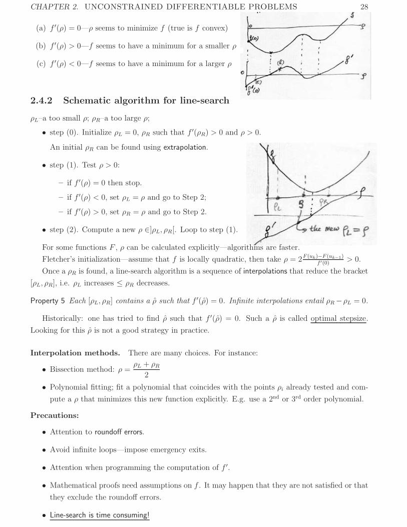
(a) f ′(ρ) = 0—ρ seems to minimize f (true is f convex)
(b) f ′(ρ) > 0—f seems to have a minimum for a smaller ρ
(c) f ′(ρ) < 0—f seems to have a minimum for a larger ρ
2.4.2 Schematic algorithm for line-search
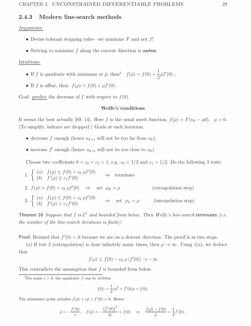
ρL–a too small ρ; ρR–a too large ρ;
• step (0). Initialize ρL = 0, ρR such that f ′(ρR) > 0 and ρ > 0.
An initial ρR can be found using extrapolation.
• step (1). Test ρ > 0:
– if f ′(ρ) = 0 then stop.
– if f ′(ρ) < 0, set ρL = ρ and go to Step 2;
– if f ′(ρ) > 0, set ρR = ρ and go to Step 2.
• step (2). Compute a new ρ ∈]ρL, ρR[. Loop to step (1).
For some functions F , ρ can be calculated explicitly—algorithms are faster.
Fletcher’s initialization—assume that f is locally quadratic, then take ρ = 2F (uk)−F (uk−1)
f ′(0) > 0.
Once a ρR is found, a line-search algorithm is a sequence of interpolations that reduce the bracket
[ρL, ρR], i.e. ρL increases ≤ ρR decreases.
Property 5 Each [ρL, ρR] contains a ρ such that f ′(ρ) = 0. Infinite interpolations entail ρR−ρL = 0.
Historically: one has tried to find ρ such that f ′(ρ) = 0. Such a ρ is called optimal stepsize.
Looking for this ρ is not a good strategy in practice.
Interpolation methods. There are many choices. For instance:
• Bissection method: ρ =ρL + ρR
2
• Polynomial fitting; fit a polynomial that coincides with the points ρi already tested and com-
pute a ρ that minimizes this new function explicitly. E.g. use a 2nd or 3rd order polynomial.
Precautions:
• Attention to roundoff errors.
• Avoid infinite loops—impose emergency exits.
• Attention when programming the computation of f ′.
• Mathematical proofs need assumptions on f . It may happen that they are not satisfied or that
they exclude the roundoff errors.
• Line-search is time consuming!
CHAPTER 2. UNCONSTRAINED DIFFERENTIABLE PROBLEMS 29
2.4.3 Modern line-search methods
Arguments:
• Devise tolerant stopping rules—we minimize F and not f !
• Striving to minimize f along the current direction is useless.
Intuitions:
• If f is quadratic with minimum at ρ, then3 f(ρ) = f(0) +1
2ρf ′(0) ;
• If f is affine, then f(ρ) = f(0) + ρf ′(0) .
Goal: predict the decrease of f with respect to f(0).
Wolfe’s conditions
It seems the best actually [69, 14]. Here f is the usual merit function, f(ρ) = F (uk − ρd), ρ > 0.
(To simplify, indexes are dropped.) Goals at each iteration:
• decrease f enough (hence uk+1 will not be too far from uk);
• increase f ′ enough (hence uk+1 will not be too close to uk).
Choose two coefficients 0 < c0 < c1 < 1, e.g. c0 < 1/2 and c1 > 1/2. Do the following 3 tests:
1.
{(a) f(ρ) ≤ f(0) + c0 ρf
′(0)(b) f ′(ρ) ≥ c1f
′(0)⇒ terminate
2. f(ρ) > f(0) + c0 ρf′(0) ⇒ set ρR = ρ (extrapolation step)
3.
{(a) f(ρ) ≤ f(0) + c0 ρf
′(0)(b) f ′(ρ) < c1f
′(0)⇒ set ρL = ρ (interpolation step)
Theorem 18 Suppose that f is C1 and bounded from below. Then Wolfe’s line-search terminates (i.e.
the number of the line-search iterations is finite).
Proof. Remind that f ′(0) < 0 because we are on a descent direction. The proof is in two steps.
(a) If test 2 (extrapolation) is done infinitely many times, then ρ → ∞. Using 1(a), we deduce
that
f(ρ) ≤ f(0)− c0 ρ |f ′(0)| → −∞This contradicts the assumption that f is bounded from below.
3For some c > 0, the quadratic f can be written
f(t) =1
2cρ2 + f ′(0)ρ+ f(0).
The minimizer point satisfies f(ρ) = cρ+ f ′(0) = 0. Hence
ρ = −f ′(0)c
, f(ρ) = −(f ′(0)
)22c
+ f(0) ⇒ f(ρ)− f(0)
ρ=
1
2f ′(0) .
CHAPTER 2. UNCONSTRAINED DIFFERENTIABLE PROBLEMS 30
Hence the number of extrapolations is finite.
(b) Suppose now that test 3 (interpolation) is done infinitely many times. Then the two sequences
{ρL} and {ρR} are adjacent and have a common limit ρ. Passing to the limit in 2 and 3(a) yields
f(ρ) = f(0) + c0 ρf′(0). (2.16)
By test 2, no ρR can be equal to ρ: indeed 2 means that ρR > ρ. Using that f ′(0) < 0 and (2.16),
test 2 can be put in the form
f(ρR) > f(0) + c0f′(0)
(ρ+ (ρR − ρ)
)= f(ρ)− c0 |f ′(0)| (ρR − ρ)
Hence
f(ρR)− f(ρ) > −c0 |f ′(0)| (ρR − ρ)Divide both sides by ρR − ρ > 0
f(ρR)− f(ρ)ρR − ρ > −c0 |f ′(0)|
For ρR ↘ ρ, the above inequality yields f ′(ρ) ≥ −c0|f ′(0)| > −c1|f ′(0)|. On the other hand, test
3(b) for ρL ↗ ρ entails f ′(ρ) ≤ −c1|f ′(0)|. The last two inequalities are contradictory.
It is impossible to repeat steps 1 and 3 alternatively neither. Hence the number of line-search
iterations is finite. �
Wolfe’s line search can be combined with any kind of descent direction −d. However, line searchis helpless if −dk is too orthogonal to ∇F (uk). The angle θk between the direction and the gradient
is crucial. Put
cos θk =〈∇F (uk), dk〉‖∇F (uk)‖ ‖dk‖ (2.17)
We can say that −dk is a “definite” descent direction if cos θk > 0 is large enough.
Theorem 19 If ∇F (u) is Lipschitz-continuous with constant � on {u : F (u) ≤ F (u0)} and the mini-
mization algorithm uses Wolfe’s rule, then
r(cos θk)2‖∇F (uk)‖2 ≤ F (uk)− F (uk+1), ∀k ∈ N, (2.18)
where the constant r > 0 is independent of k.
Proof. Note that condition 1 in Wolfe’s rule corresponds to a descent scenario. By the expression
for cos(θk) in (2.17) and using that uk+1 = uk − ρkdk we get
ρkf′(0) = −ρk 〈∇F (uk), dk〉 = − cos(θk)‖∇F (uk)‖ ‖ρkdk‖ = − cos(θk)‖∇F (uk)‖ ‖uk − uk+1‖ < 0.
Combining this result with condition 1(a) yields
0 < c0 ρk|f ′(0)| = c0 cos(θk)‖∇F (uk)‖ ‖uk − uk+1‖ ≤f(0)− f(ρk) = F (uk)− F (uk+1) (2.19)
Note that F (uk)− F (uk+1) is bounded from below by a positive number (descent is guaranteed by
test 1). Reminding that f(ρk) = F (uk − ρkdk) = F (uk+1), condition 1(b) reads
f ′(ρk) = −〈∇F (uk+1), dk〉 ≥ c1f′(0) = −c1 〈∇F (uk), dk〉
CHAPTER 2. UNCONSTRAINED DIFFERENTIABLE PROBLEMS 31
Add 〈∇F (uk), dk〉 to both sides of the above inequality:
−〈∇F (uk+1)−∇F (uk), dk〉 ≥ (1− c1) 〈∇F (uk), dk〉 .Using Schwarz’s inequality and the definition of cos(θk),
‖∇F (uk+1)−∇F (uk)‖ ‖dk‖ ≥ (1− c1) cos(θk)‖∇F (uk)‖ ‖dk‖.Division of both sides by ‖dk‖ �= 0 leads to
‖∇F (uk+1)−∇F (uk)‖ ≥ (1− c1) cos(θk)‖∇F (uk)‖Combining this result with the Lipschitz property, i.e. ‖∇F (uk+1)−∇F (uk)‖ ≤ �‖uk+1−uk‖, yields
�‖uk+1 − uk‖ ≥ ‖∇F (uk+1)−∇F (uk)‖ ≥ (1− c1) cos(θk)‖∇F (uk)‖Multiplying both sides by cos(θk)‖∇F (uk)‖ and using (2.19) for the underlined term below leads to
(1− c1)(cos(θk)
)2‖∇F (uk)‖2 ≤ �
c0
(c0 cos(θk)‖∇F (uk)‖ ‖uk+1 − uk‖
)≤ �
c0
(F (uk)− F (uk+1)
).
For
r =c0(1− c1)
�> 0
we obtain
r(cos(θk)
)2‖∇F (uk)‖2 ≤ F (uk)− F (uk+1).
The proof is complete. �
Why in the proof we use only test 1 ?
Theorem 20 Let F ∼ C1 be bounded from below. Assume that the iterative scheme is such that (2.18),
namely
r(cos θk)2‖∇F (uk)‖2 ≤ F (uk)− F (uk+1), ∀k ∈ N,
holds true for a constant r > 0 independent of k. If the series
∞∑k=0
(cos θk)2 diverges (2.20)
then limk→∞∇F (uk) = 0.
Proof. Since(F (uk)
)k∈N is decreasing and bounded from below, there is a finite number F ∈ R
such that F (uk) ≥ F , ∀k ∈ N. Then (2.18) yields
∞∑k=0
(cos θk)2‖∇F (uk)‖2 ≤ 1
r
∞∑k=0
(F (uk)− F (uk+1)
)=
1
r
(F (u0)− F (u1) + F (u1)− F (u2) + · · ·
)≤ 1
r
(F (u0)− F
)< +∞. (2.21)
If there was δ > 0 such that ‖∇F (uk)‖ ≥ δ, ∀k ≥ 0, then (2.20) would yield
∞∑k=0
(cos θk)2‖∇F (uk)‖2 ≥ δ2
∞∑k=0
(cos θk)2 →∞
which contradicts (2.21). Hence the conclusion. �
Property (2.20) depends on the way the direction is computed.
CHAPTER 2. UNCONSTRAINED DIFFERENTIABLE PROBLEMS 32
Remark 8 Wolfe’s rule needs to compute the value of f ′(ρ) = −〈∇F (uk − ρdk), dk〉 at each cycle of
the line-search. Computing ∇F (uk−ρdk) is costly when compared to the computation of F (uk−ρdk).Other line-search methods avoid the computation of ∇F (uk − ρdk).
Other Line-Searches
We can evoke e.g. the Goldstein and Price method and the Armijo’s method. More details: e.g.
[69, 14].
Armijo’s methods
Choose c ∈ (0, 1). Tests for ρ:
1. f(ρ) ≤ f(0) + cρf ′(0) ⇒ terminate;
2. f(ρ) > f(0) + cρf ′(0) ⇒ set ρR = ρ.
It is easy to see that this line-search terminates as well. The interest of the method is that it does
not need to compute f ′(ρ). It ensures that ρ is not too large. However, it can be dangerous since it
never increases ρ; thus it relies on the initial step-size ρ0.
In practice it often had appeared that taking a good constant step-size yields a faster convergence.
2.5 Second-order methods
Based on F (uk+1)− F (uk) ≈ 〈∇F (uk), uk+1 − uk〉+ 12〈∇2F (uk)(uk+1 − uk), uk+1 − uk〉
Crucial approach to derive a descent direction at each iteration of a scheme minimizing a smooth
objective F .
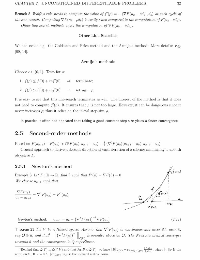
2.5.1 Newton’s method
Example 3 Let F : R→ R, find u such that F ′(u) = ∇F (u) = 0.
We choose uk+1 such that:
∇F (uk)uk − uk+1
= ∇2F (uk) = F′′(uk)
Newton’s method: uk+1 = uk −(∇2F (uk)
)−1∇F (uk) (2.22)
Theorem 21 Let V be a Hilbert space. Assume that ∇2F (uk) is continuous and invertible near u,
say O " u, and that4∥∥∥(∇2F (u)
)−1∥∥∥L(V )
is bounded above on O. The Newton’s method converges
towards u and the convergence is Q-superlinear.
4Remind that L(V ) ≡ L(V, V ) and that for B ∈ L(V ), we have ‖B‖L(V ) = supu∈V \{0}‖Bu‖V
‖u‖V, where ‖ · ‖V is the
norm on V . If V = Rn, ‖B‖L(V ) is just the induced matrix norm.
CHAPTER 2. UNCONSTRAINED DIFFERENTIABLE PROBLEMS 33
Proof. Using Taylor expansion for ∇F about uk:
0 = ∇F (u) = ∇F (uk) +∇2F (uk) (u− uk) + ‖u− uk‖ε(u− uk) = 0,
where ε(u− uk)→ 0 as ‖u− uk‖ → 0. By Newton’s method (2.22),
∇F (uk) +∇2F (uk) (uk+1 − uk) = 0
Subtracting this equation from the previous one yields
∇2F (uk) (u− uk+1) + ‖u− uk‖ε(u− uk) = 0.
Since ∇2F (uk) is invertible, the latter equation is equivalent to
u− uk+1 = −(∇2F (uk)
)−1‖u− uk‖ε(u− uk).
From the assumptions, the constant M below is finite:
Mdef= sup
u∈O(u)
∥∥∥(∇2F (u))−1
∥∥∥L(V )
.
Then
‖uk+1 − u‖ ≤M‖u − uk‖ε(u− uk)and Qk =
‖uk+1−u‖‖u−uk‖ ≤ Mε(u − uk) → 0 as ‖u − uk‖ → 0. Hence the Q-superlinearity of the
convergence. �
Comments
• Under the conditions of the theorem, if in addition F is C3 then convergence is Q-quadratic.
• Direction and step-size are automatically chosen (−(∇2F (uk))−1∇F (uk));
• If F is nonconvex, −(∇2F (uk))−1∇F (uk) may not be a descent direction, hence the u found
in this way is not necessarily a minimizer if F ;
• Convergence is very fast;
• Computing(∇2F (uk)
)−1can be difficult, i.e. solving the equation ∇2F (uk)z = ∇F (uk) with
respect to z can require a considerable computational effort;
Numerically it can be very unstable thus entailing a violent divergence;
• Preconditioning can help if ∇2F (uk) has a favorable structure, see [19];
• In practice—efficient to get a high-precision u if we are close enough to the sought-after u.
CHAPTER 2. UNCONSTRAINED DIFFERENTIABLE PROBLEMS 34
2.5.2 General quasi-Newton Methods
Approximation :(Hk(uk)
)−1 ≈(∇2F (uk)
)−1
uk+1 = uk −(Hk(uk)
)−1∇F (uk) (2.23)
Possible to keep H−1k (uk) constant for several consecutive iterations.
Sufficient conditions for convergence:
Theorem 22 F : U ⊂ V → R twice differentiable in O(U), V complete n.v.s. Suppose there exist
constants r > 0, M > 0 and γ ∈]0, 1[ such that Bdef= B(u0, r) ⊂ U and
1. supk∈N
supu∈B‖H−1
k (u)‖L(V ) ≤M
2. supk∈N
supu,v∈B
‖∇2F (u)−Hk(v)‖L(V ) ≤ γ
M
3. ‖∇F (u0)‖V ≤ r
M(1− γ)
Then the sequence generated by (2.23) satisfies:
(i) uk ∈ B, ∀k ∈ N;
(ii) limk→∞
uk → u; moreover, u is the unique zero of ∇F (u) on B;
(iii) The convergence is geometric with
‖uk − u‖V ≤ γk
(1− γ)‖u1 − u0‖V .
Proof. We will use that iteration (2.23) is equivalent to
Hk(uk)(uk+1 − uk
)+∇F (uk) = 0, ∀k ∈ N. (2.24)
There are several steps.
(a) We will show 3 preliminary results:
‖uk+1 − uk‖ ≤M‖∇F (uk)‖, ∀k ∈ N; (2.25)
uk+1 ∈ B, ∀k ∈ N ; (2.26)
‖∇F (uk+1)‖ ≤ γ
M‖uk+1 − uk‖. (2.27)
We start with k = 0. Iteration (2.23) yields (2.25) and (2.26) for k = 1:
‖u1 − u0‖ ≤‖H−10 (u0)‖ ‖∇F (u0)‖ ≤M ‖∇F (u0)‖ ≤M
r
M(1− γ) < r ⇒ u1 ∈ B
Using (2.24) for k = 0,
∇F (u1) = ∇F (u1)−∇F (u0)−H0(u0)(u1 − u0
)
CHAPTER 2. UNCONSTRAINED DIFFERENTIABLE PROBLEMS 35
Consider the application u �→ ∇F (u) − H0(u0)u. Its gradient is ∇2F (u) − H0(u0). By the
generalized mean-value theorem 5 and assumption 2 we obtain (2.27) for k = 1:
‖∇F (u1)−H0(u0)u1 −∇F (u0) +H0(u0)u0‖= ‖∇F (u1)‖ ≤ sup
u∈B‖∇2F (u)−H0(u0)‖ ‖u1 − u0‖
≤ γ
M‖u1 − u0‖.
Suppose that (2.25)-(2.27) hold till (k − 1) inclusive, which means we have
‖uk − uk−1‖ ≤M‖∇F (uk−1)‖uk ∈ B;
‖∇F (uk)‖ ≤ γ
M‖uk − uk−1‖
(2.28)
We check if these hold for k as well. Using (2.28) and assumption 1, iteration (2.23) yields
(2.25):
‖uk+1 − uk‖ ≤‖H−1k (uk)‖ ‖∇F (uk)‖ ≤M ‖∇F (uk)‖ ≤M
γ
M‖uk − uk−1‖ = γ‖uk − uk−1‖
Thus we have established that
‖uk+1 − uk‖ ≤ γ‖uk − uk−1‖ ≤ · · · ≤ γk‖u1 − u0‖ (2.29)
Using the triangular inequality, (2.25) for k = 0 and assumption 3, we get (2.26) for the
actual k:
‖uk+1 − u0‖ ≤ ‖uk+1 − uk‖+ ‖uk − uk−1‖+ · · ·+ ‖u1 − u0‖ =k∑
i=0
‖ui+1 − ui‖
≤(
k∑i=0
γi
)‖u1 − u0‖ ≤
( ∞∑i=0
γi
)‖u1 − u0‖ = 1
1− γ ‖u1 − u0‖
≤ M‖∇F (u0)‖1− γ ≤ r ⇒ uk+1 ∈ B.
Using (2.24) yet again
∇F (uk+1) = ∇F (uk+1)−∇F (uk)−Hk(uk)(uk+1 − uk
)Applying in a similar way the generalized mean-value theorem to the application u �→ ∇F (u)−Hk(uk)u and using assumption 2 entails (2.27):
‖∇F (uk+1)‖ ≤ supu∈B‖∇2F (u)−Hk(uk)‖ ‖uk+1 − uk‖≤ γ
M‖uk+1 − uk‖.
5Generalized mean-value theorem. Let f : U ⊂ V → W and a ∈ U , b ∈ U such that the segment [a, b] ∈ U .Assume f is continuous on [a, b] and differentiable on ]a, b[. Then
‖f(b)− f(a)‖W ≤ supu∈]a,b[
‖∇f(u)‖L(V,W )‖b− a‖V
CHAPTER 2. UNCONSTRAINED DIFFERENTIABLE PROBLEMS 36
(b) Let us prove the existence of a zero of ∇F in B. Using (2.29), ∀k ∈ N, ∀j ∈ N we have
‖uk+j−uk‖ ≤j−1∑i=0
‖uk+i+1−uk+i‖ ≤j−1∑i=0
γk+i‖u1−u0‖ ≤ γk‖u1−u0‖∞∑i=0
γi =γk
1− γ ‖u1−u0‖,(2.30)
hence (uk)k∈N is a Cauchy sequence. The latter, combined with the fact that B ⊂ V is complete
shows that ∃ u ∈ B such that limk→∞
uk = u.
(c) Since ∇F is continuous on O(U) ⊃ B and using (2.27), we obtain the existence result:
‖∇F (u)‖ = limk→∞‖∇F (uk)‖ ≤ γ
Mlimk→∞‖uk+1 − uk‖ = 0
(d) Uniqueness of u in B.
Suppose ∃u ∈ B, u �= u such that ∇F (u) = 0 = ∇F (u). We can hence write
u− u = −H−10 (u0)
(∇F (u)−∇F (u)−H0(u0) (u− u)
)‖u− u‖ ≤ ‖H−1
0 (u0)‖ supu∈B‖∇2F (u)−H0(u0)‖ ‖u− u‖ ≤M
γ
M‖u− u‖< ‖u− u‖
This is impossible, hence u is unique in B.
(e) Geometric convergence: using (2.30),
‖u− uk‖ = limj→∞‖uk+j − uk‖ ≤ γk
1− γ ‖u1 − u0‖. �
Iteration (2.23) is quite general. In particular, Newton’s method (2.22) corresponds to Hk(uk) =
∇2F (uk) while (variable) stepsize Gradient descent to Hk(uk) =1ρkI.
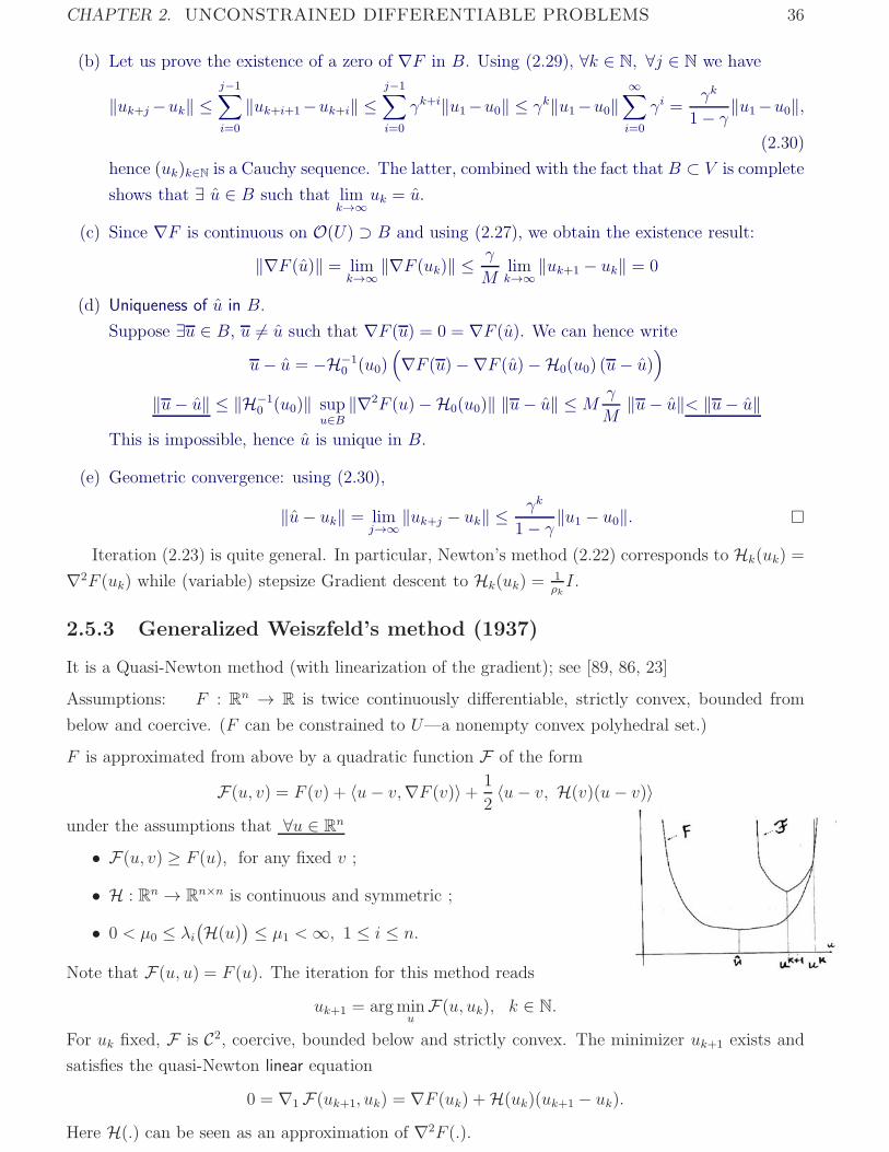
2.5.3 Generalized Weiszfeld’s method (1937)
It is a Quasi-Newton method (with linearization of the gradient); see [89, 86, 23]
Assumptions: F : Rn → R is twice continuously differentiable, strictly convex, bounded from
below and coercive. (F can be constrained to U—a nonempty convex polyhedral set.)
F is approximated from above by a quadratic function F of the form
F(u, v) = F (v) + 〈u− v,∇F (v)〉+ 1
2〈u− v, H(v)(u− v)〉
under the assumptions that ∀u ∈ Rn
• F(u, v) ≥ F (u), for any fixed v ;
• H : Rn → Rn×n is continuous and symmetric ;
• 0 < μ0 ≤ λi(H(u)) ≤ μ1 <∞, 1 ≤ i ≤ n.
Note that F(u, u) = F (u). The iteration for this method reads
uk+1 = argminuF(u, uk), k ∈ N.
For uk fixed, F is C2, coercive, bounded below and strictly convex. The minimizer uk+1 exists and
satisfies the quasi-Newton linear equation
0 = ∇1F(uk+1, uk) = ∇F (uk) +H(uk)(uk+1 − uk).Here H(.) can be seen as an approximation of ∇2F (.).

CHAPTER 2. UNCONSTRAINED DIFFERENTIABLE PROBLEMS 37
2.5.4 Half-quadratic regularization
Minimize F : Rn → R of the form
F (u) = ‖Au− v‖22 + β
r∑i=1
ϕ(‖Diu‖2), (2.31)
where Di ∈ Rs×n for s ∈ {1, 2}: s = 2—e.g. discrete gradients, see (1.8) and s = 1—e.g. finite
differences, see (1.9), p. 7. Let us denote
Ddef=
⎡⎢⎢⎢⎣D1
D2...Dr
⎤⎥⎥⎥⎦ ∈ Rrs×n. Assumption: ker(ATA) ∩ ker(DTD) = {0}.
Furthermore, ϕ : R+ → R is a convex edge-preserving potential function (see [7]), e.g.
ϕ ϕ′ ϕ′′√t2 + α
t√α + t2
α
(√α + t2)3
α log
(cosh
(t
α
))tanh
(t
α
) (1− tanh2
(t
α
))1
α
|t| − α log
(1 +|t|α
)t
α + |t|α
(α+ |t|)2{t2/2 if |t| ≤ α,α|t| − α2/2 if |t| > α,
{t if |t| ≤ α,αsign(t) if |t| > α,
{1 if |t| ≤ α,0 if |t| > α,
|t|α, 1 < α ≤ 2 α|t|α−1sign(t) α(α− 1)|t|α−2
where α > 0 is a parameter. Note that F is differentiable.
However ϕ′ is (nearly) bounded, so ϕ′′ is close to zero on large regions; if A is not well conditioned
(a common case in practice), ∇2F has nearly null regions and convergence of usual methods can be
extremely slow. Newton’s method reads uk+1 = uk − (∇2F (uk)))−1∇F (uk). E.g., for s = 1 we have
Diu ∈ R, so ‖Diu‖2 = |Diu| and
∇2F (u) = 2ATA+ βr∑
i=1
ϕ′′(|Diu|)DTi Di.
For the class of F considered here, ∇2F (u) has typically a bad condition number so (∇2F (u)−1) is
difficult (unstable) or impossible to obtain numerically. Newton’s method is practically unfeasible.
Half-quadratic regularization, two forms multiplicative (“×”) and additive (“+”) introduced in [42]
and [43], respectively. Main idea: using an auxiliary variable b, construct an augmented criterion
F(u, b) which is quadratic in u and separable in b, such that
(u, b) = argminu,bF(u, b) ⇒ u = argmin
uF (u)
Alternate minimization: ∀k ∈ N,
⎧⎪⎨⎪⎩uk+1 = argmin
uF(u, bk)
bk+1[i] = argminbF(uk+1, b), 1 ≤ i ≤ r .
The construction of these augmented criteria rely on Theorem 4 (Fenchel-Moreau, p. 15).
CHAPTER 2. UNCONSTRAINED DIFFERENTIABLE PROBLEMS 38
Multiplicative form.
Usual assumptions on ϕ in order to guarantee global convergence:
(a) t→ ϕ(t) is convex and increasing on R+, ϕ �≡ 0 and ϕ(0) = 0
(b) t→ ϕ(√t) is concave on R+,
(c) ϕ is C1 on R+ and ϕ′(0) = 0,(d) ϕ′′(0+) > 0,(e) lim
t→∞ϕ(t)/t2 = 0.
Proposition 1 We have
ψ(b) = supt∈R
{−12bt2 + ϕ(t)
}⇔ ϕ(t) = min
b≥0
(1
2t2b+ ψ(b)
)(2.32)
Moreover, bdef=
{ϕ′(t)t
if t > 0
ϕ′′(0+) if t = 0is the unique point yielding ϕ(t) = 1
2t2b+ ψ(b).
The proof of the proposition is outlined in Appendix, p. 106.
Based on Proposition 1 we minimize w.r.t. (u, b) an F of the form given below
F(u, b) = ‖Au− v‖22 + βr∑
i=1
(b[i]
2‖Diu‖22 + ψ(b[i])
)and iterates read, for k ∈ N:
uk+1 = (H(bk))−1 2ATv, H(b) = 2ATA+ β
r∑i=1
b[i]DTi Di
bk+1[i] =ϕ′(‖Diuk+1‖2)‖Diuk+1‖2 , 1 ≤ i ≤ r.
Comments
• References [24, 34, 47, 7, 68, 1].
• Interpretation : bk edge variable (≈ 0 if “discontinuity”)
• uk can be computed efficiently using CG (see § 2.6).
• F is nonconvex w.r.t. (u, b). However, under (a)-(e) the minimum is unique and convergence
is ensured, uk → u (see [68, 1]).
• Quasi-Newton : uk+1 = uk − (H(uk))−1∇F (uk), H(u) = H
((ϕ′(‖Diu‖2)‖Diu‖2
)r
i=1
)� 0
Compare with H in Newton.
• Iterates amount to the relaxed fixed point iteration described next. In order to solve the equation
∇F (u) = 0, we write
∇F (u) = L(u)u− zwhere z is independent of u. At each iteration k, one finds uk+1 by solving the linear problem
L(uk)uk+1 = z
In words, ∇F is linearized at each iteration (see [67] for the proof).
CHAPTER 2. UNCONSTRAINED DIFFERENTIABLE PROBLEMS 39
Additive form.
Usual assumptions on ϕ to ensure convergence:
(a) t→ ϕ(t) is convex and increasing on R+, ϕ �≡ 0 and ϕ(0) = 0(b) t→ t2/2− ϕ(t) is convex,(c) ϕ′(0) = 0,(d) lim
t→∞ϕ(t)/t2 < 1/2.
Notice that ϕ is differentiable on R+. Indeed, (a) implies that ϕ′(t−) ≤ ϕ′(t+), for all t. If for some t
the latter inequality is strict, (b) cannot be satisfied. If follows that ϕ′(t−) = ϕ′(t+) = ϕ′(t).
In order to avoid additional notations, we write ϕ(‖.‖) and ψ(‖.‖) next.Proposition 2 For ‖.‖ = ‖.‖2 and b ∈ R
s, t ∈ Rs, s ∈ {1, 2}, we have the equivalence:
ψ(‖b‖) = maxt∈Rs
{−12‖b− t‖2 + ϕ(‖t‖)
}⇔ ϕ(‖t‖) = min
b∈Rs
(1
2‖t− b‖2 + ψ(‖b‖)
)(2.33)
Moreover, bdef= t− ϕ′(‖t‖) t
‖t‖ is the unique point yielding ϕ(‖t‖) = 12‖t− b‖2 + ψ(‖b‖).
Proof. By (b) and (d),(12‖t‖2 − ϕ(‖t‖)) is convex and coercive, so the maximum of ψ is reached.
The formula for ψ in (2.33) is equivalent to
ψ(‖b‖) + 1
2‖b‖2 = max
t∈Rs
{〈b, t〉 −
(1
2‖t‖2 − ϕ(‖t‖)
)}(2.34)
The term on the left is the convex conjugate of 12‖t‖2−ϕ(‖t‖), see (1.10), p. 14. The latter term being
convex continuous and �≡ ∞, using convex bi-conjugacy (Theorem 4, p. 15), (2.34) is equivalent to
1
2‖t‖2 − ϕ(‖t‖) = sup
b∈Rs
{〈b, t〉 −
(ψ(‖b‖) + 1
2‖b‖2
)}(2.35)
Noticing that the supremum in (2.35) is reached, (2.35) is equivalent to
ϕ(‖t‖) = minb∈Rs
{−〈b, t〉+
(ψ(‖b‖) + 1
2‖b‖2
)+
1
2‖t‖2
}= min
b∈Rs
(1
2‖t− b‖2 + ψ(‖b‖)
)Hence (2.33) is proven.
Using (2.33), the maximum of ψ and the minimum of ϕ are reached by a pair (t, b) such that
b− t+ ϕ′(‖t‖) t
‖t‖ = 0.
For t fixed, the solution for b, denoted b is unique and is as stated in the proposition. �
Based on Proposition 2, we consider
F(u, b) = ‖Au− v‖22 + βr∑
i=1
(1
2‖Diu− bi‖2s + ψ(bi)
), bi ∈ R
s (2.36)
and the iterations read, ∀k ∈ N,
uk+1 = H−1
(2ATv + β
r∑i=1
DTi bik
), H = 2ATA + β
r∑i=1
DTi Di
bik+1= Diuk − ϕ′(‖Diuk‖2) Diuk
‖Diuk‖2 , 1 ≤ i ≤ r.
CHAPTER 2. UNCONSTRAINED DIFFERENTIABLE PROBLEMS 40
Comments
• References: [8, 47, 68, 1].
• Quasi-Newton : uk+1 = uk −H−1∇F (u) (compare with ∇2F )
• Convergence: uk → u.
Comparison between the two forms. See [68].
• “ × ′′-form: less iterations but each iteration is expensive;
• “ + ′′-form: more iterations but each iteration is cheaper and it is possible to precondition H.
• For both forms, convergence is faster than Gradient, DFP and BFGC (§ 2.5.5), and non-linear
CG (§ 2.6.2) for functions of the form (2.31).
2.5.5 Standard quasi-Newton methods
References: [14, 54, 69]. Here F : Rn → R with ‖u‖ = √〈u, u〉, ∀u ∈ Rn.
Hk ≈ ∇2F (uk) � 0 and Mk ≈(∇2F (uk)
)−1 � 0, ∀k ∈ N.
Δkdef= uk+1 − uk
gkdef= ∇F (uk+1)−∇F (uk)
Definition 14 Quasi-Newton (or secant) equation:
Mk+1gk = Δk (2.37)
Interpretation: the mean value H of ∇2F between uk and uk+1 satisfies gk = HΔk. So (2.37) forces
Mk+1 to have the same action as H−1 on gk (subspace of dimension one).
There are infinitely many quasi-Newton matrices satisfying Definition 14.
General quasi-Newton scheme
0. Fix u0, tolerance ε � 0, M0 � 0 such that M0 =MT0 . If ‖∇F (u0)‖ ≤ ε stop, else go to 1.
For k = 1, 2, . . ., do:
1. dk =Mk∇F (uk)
2. Line search along −dk to find ρk (e.g. Wolfe, ρ0 = 1)
3. uk+1 = uk − ρkdk4. if ‖∇F (uk+1)‖ ≤ ε stop else go to step 5
5. Mk+1 =Mk + Ck � 0 so that Mk+1 =MTk+1 and (2.37) holds; then loop to step 1
Ck � 0 is a correction matrix. For stability and simplicity, it should be “minimal” in some sense.
Various choices for Ck can be done.
CHAPTER 2. UNCONSTRAINED DIFFERENTIABLE PROBLEMS 41
DFP (Davidon-Fletcher-Powel)
Historically the first (1959). Apply the General quasi-Newton scheme along with
Mk+1 = Mk + Ck
Ck =ΔkΔ
Tk
gTk Δk
− Mkgk gTkMk
gTkMkgk
Each of the matrices composing Ck is of rank ≤ 1, hence rankCk ≤ 2, ∀k ∈ N. Note that Ck = CTk .
Mk+1 is symmetric and satisfies the quasi-Newton equation (2.37):
Mk+1gk =Mkgk +ΔkΔT
k gkgTk Δk
−MkgkgTkMkgkgTkMkgk
=Mkgk +Δk −Mkgk = Δk
BFGC (Broyden-Fletcher-Goldfarb-Shanno)
Proposed in 1970. Apply the General quasi-Newton scheme along with
Mk+1 = Mk + Ck
Ck = −ΔkgTkMk +MkgkΔ
Tk
gTk Δk
+
(1 +
gTkMkgkgTk Δk
)ΔkΔ
Tk
gTk Δk
Obviously Mk+1 satisfies (2.37) as well. BFGC is often preferred to DFP.
Comment: One can approximate ∇2F using Hk+1 = Hk+ Ck where Hk must satisfy the so called
“dual” quasi-Newton equation, Hk+1Δk = gk, ∀k (see [14, p. 55]).
Theorem 23 Let M0 � 0 (resp. H0 � 0). Then gTk Δk > 0 is a necessary and sufficient condition for
DFP and BFGS formulae to give Mk � 0 (resp. Hk � 0), ∀k ∈ N.
Proof—see [14, p. 56.]
Remark 9 It can be shown that DFP and BFGC formulae are mutually dual. See [14, p. 56].
Theorem 24 Let F be convex, bounded from below and ∇F Lipschitzian on {u : F (u) ≤ F (u0)}.Then the BFGS algorithm with Wolfe’s line-search and M0 � 0, M0 =MT
0 yields
lim infk→∞
|∇F (uk)| = 0.
Proof—see [14, p. 58.]
• Locally - Q superlinear convergence;
• Drawback: we have to store n× n matrices;
• DFP, BFGC available in Matlab Optimization toolbox.
Recently the BFGS minimization method was extended in [49] to handle nonsmooth, not necessarily
convex problems. The Matlab package HANSO developed by the authors is freely available6.
6http://www.cs.nyu.edu/overton/software/hanso/
CHAPTER 2. UNCONSTRAINED DIFFERENTIABLE PROBLEMS 42
2.6 Conjugate gradient method (CG)
Due to Hestenes and Stiefel, 1952, still contains a lot of material for research.
Preconditioned CG is an important technique to solve large systems of equations.
2.6.1 Quadratic strongly convex functionals (Linear CG)
For B = BT and B � 0, powerful method to minimize F given below for n very large
F (u) =1
2〈Bu, u〉 − 〈c, u〉 , u ∈ R
n
or equivalently to solve Bu = c. (Remind that B � 0 implies λmin(B) > 0.) Then F is strongly
convex. By the definition of F , we have a very useful relation:
∇F (u− v) = B(u− v)− c = ∇F (u)− Bv, ∀u, v ∈ Rn. (2.38)
Main idea : at each iteration, compute uk+1 such that
F (uk+1) = infu∈uk+Hk
F (u)
Hk = Span{∇F (ui), 0 ≤ i ≤ k}
uk+1 minimizes F over an affine subspace (and not only along one direction, as in Gradient methods.)
Theorem 25 The CG method converges after n iterations at most and it provides the unique exact
minimiser u obeying F (u) = minu∈Rn
F (u).
Proof. Define the subspace
Hk =
{g(α) =
k∑i=0
α[i]∇F (ui) : α[i] ∈ R, 0 ≤ i ≤ k
}(2.39)
Hk is a closed convex set. Set f(α)def= F
(uk − g(α)
). Note that f is convex and coercive.
F (uk+1) = infα∈Rk+1
F(uk − g(α)
)= inf
α∈Rk+1f(α) = f(αk).
αk is the unique solution of ∇f(α) = 0. By (2.39), ∂g(α)/∂α[i] = ∇F (ui). Then∂f(α)
∂α[i]= 0 = −〈∇F (uk − g(α)) ,∇F (ui)〉 = −〈∇F (uk+1) ,∇F (ui)〉 , 0 ≤ i ≤ k. (2.40)
Hence for 0 ≤ k ≤ n− 1 we have
〈∇F (uk+1) ,∇F (ui)〉 = 0, 0 ≤ i ≤ k (2.41)
⇒ 〈∇F (uk+1) , u〉 = 0, ∀u ∈ Hk (2.42)
It follows that{∇F (ui)} are linearly independent. Conclusions about convergence:
• If ∇F (uk) = 0 then u = uk (terminate).

CHAPTER 2. UNCONSTRAINED DIFFERENTIABLE PROBLEMS 43
• If ∇F (uk) �= 0 then dimHk = k + 1.
Suppose that ∇F (un−1) �= 0, then Hn−1 = Rn. By (2.42),
〈∇F (un), u〉 = 0, ∀u ∈ Rn ⇒ ∇F (un) = 0 ⇒ u = un.
The proof is complete. �
Remark 10 In practice, numerical errors can require a higher number of iterations.
The derivation of the CG algorithm is outlined in Appendix on p. 107
CG Algorithm:
0. Initialization: d−1 = 0, ‖∇F (u−1)‖ = 1 and u0 ∈ Rn. Then for k = 0, 1, 2, · · · do:
1. if ∇F (uk) = 0 then terminate; else go to step 2
2. ξk =‖∇F (uk)‖2‖∇F (uk−1)‖2 (where ∇F (uk) = Buk − c, ∀k)
3. dk = ∇F (uk) + ξk dk−1 (by step 0, we have d0 = ∇F (u0))
4. ρk =〈∇F (uk), dk〉〈Bdk, dk〉 (where B = ∇2F (uk), ∀k)
5. uk+1 = uk − ρkdk; then loop to step 1.
Main Properties :
• ∀k, 〈∇F (uk+1),∇F (ui)〉 = 0 if 0 ≤ i ≤ k
• ∀k, 〈Bdk+1, di〉 = 0 if 0 ≤ i ≤ k— directions are conjugated w.r.t. ∇2F = B
• since B � 0 it follows that (dk)nk=1 are linearly independent where n ≤ n is such that
∇F (un) = 0.
• CG does orthogonalization: DTBD is diagonal where D = [d1, . . . , dn] (the directions).
Theorem 26 If B has only r different eigenvalues, then the CG method converges after r iterations
at most.
Proof—see [69]. Hence faster convergence if the eigenvalues of B are “concentrated”.
2.6.2 Non-quadratic Functionals (non-linear CG)
References: [69, 14]
Nonlinear variants of the CG are well studied and have proved to be quite successful in practice.
However, in general there is no guarantee to converge in a finite number of iterations.
Main idea: cumulate past information when choosing the new descent direction.

CHAPTER 2. UNCONSTRAINED DIFFERENTIABLE PROBLEMS 44
Fletcher-Reeves method (FR)
step 0. Initialization: d−1 = 0, ‖∇F (u−1)‖ = 1 and u0 ∈ Rn.
∀k ∈ N:
1. Compute ∇F (uk); if ‖∇F (uk)‖ ≤ ε then stop, otherwise go to step 2
2. ξk =‖∇F (uk)‖2‖∇F (uk−1)‖2
3. dk = ∇F (uk) + ξk dk−1
4. Test: if 〈∇F (uk), dk〉 < 0 (−dk is not a descent direction) set dk = −∇F (uk)
5. Line-search along −dk to obtain ρk > 0
6. uk+1 = uk − ρkdk, then loop to step 1.
C. Comments (see [14, p. 72])
• The new direction dk still involves memory from previous directions (”Markovian property”).
• Conjugacy has little meaning in the non-quadratic case.
• FR is heavily based on the locally quadratic shape of F (only step 4 is new w.r.t. CG).
• If the line-search is exact, the new direction −dk is a descent direction.
Polak-Ribiere (PR) method
Remark 11 There are many variants of the FR method that differ from each other mainly in the
choice of the parameter ξk. An important variant is the PR method.
By the mean-value formula there is ρ ∈]0, ρk−1] such that along the line Span(dk−1) we have
∇F (uk) = ∇F (uk−1)− ρk−1Bk dk−1 (2.43)
for Bk = ∇2F (uk−1 − ρdk−1) (2.44)
Note that Bk = BTk .
Main idea: choose a ξk in the FR method that conjugates dk and dk−1 w.r.t. Bk, i.e. that yields
〈Bkdk−1 , dk〉 = 0.
However, Bk is unknown. By way of compromise, the result given below will be used.
Lemma 2 Let Bk be given by (2.43)-(2.44) and consider the FR methods where
(i) ξk =〈∇F (uk)−∇F (uk−1),∇F (uk)〉
‖∇F (uk−1)‖2 (the PR formula)
(ii) ρk−1 and ρk−2 are optimal.

CHAPTER 2. UNCONSTRAINED DIFFERENTIABLE PROBLEMS 45
Then 〈Bkdk−1 , dk〉 = 0.
Proof. By (2.43), we have −Bk dk−1 =1ρk(∇F (uk)−∇F (uk−1)). Then we can write
〈−Bkdk−1,∇F (uk)〉〈Bkdk−1, dk−1〉 =
⟨(∇F (uk)−∇F (uk−1)),∇F (uk)
⟩⟨(−∇F (uk) +∇F (uk−1)), dk−1
⟩ =
⟨(∇F (uk)−∇F (uk−1)),∇F (uk)
⟩−〈∇F (uk), dk−1〉+ 〈∇F (uk−1), dk−1〉
If ρk−1 is optimal, i.e. if F (uk−1 − ρkdk−1) = infρ F (uk−1 − ρdk−1), then
〈∇F (uk−1 − ρk−1dk−1), dk−1〉 = 0 = 〈∇F (uk), dk−1〉
Then〈−Bkdk−1,∇F (uk)〉〈Bkdk−1, dk−1〉 =
⟨(∇F (uk)−∇F (uk−1)),∇F (uk)
⟩〈∇F (uk−1), dk−1〉
If ρk−2 is optimal as well, in the same way we have 〈∇F (uk−1), dk−2〉 = 0. Using this result and the
formula for dk−1 according to step 3 in PR, the denominator on the right hand side is
〈∇F (uk−1), dk−1〉 = 〈∇F (uk−1),∇F (uk−1) + ξk−1dk−2〉 = ‖∇F (uk−1)‖2.
It follows that 〈−Bkdk−1,∇F (uk)〉〈Bkdk−1, dk−1〉 = ξk
for ξk as in the Lemma. Using the expression for ξk established above, we find:
〈Bkdk−1 , dk〉 = 〈Bkdk−1 , ∇F (uk) + ξkdk−1〉 = 〈Bkdk−1 , ∇F (uk)〉+ ξk 〈Bkdk−1 , dk−1〉= 〈Bkdk−1 , ∇F (uk)〉 − 〈Bkdk−1,∇F (uk)〉
〈Bkdk−1, dk−1〉 〈Bkdk−1 , dk−1〉 = 0.
Hence the result. �
PR method
Apply the FR method, p. 44, where ξk in step 2 is replaced by the PR formula
ξk =〈∇F (uk)−∇F (uk−1),∇F (uk)〉
‖∇F (uk−1)‖2 .
Comparison between FR and PR (see [14, p. 75])
• FR converges globally (F convex, coercive).
• There is a counter-example where PR does not converge
• PR converges if F is locally strongly convex
• PR converges much faster than FR (so the latter is rarely used in practice)
• Relation with quasi-Newton

CHAPTER 2. UNCONSTRAINED DIFFERENTIABLE PROBLEMS 46
2.6.3 Condition number and preconditioning
Example 4 Consider the linear system (example due to R.S.Wilson):
Au = v
where
A =
⎡⎢⎢⎣10 7 8 77 5 6 58 6 10 97 5 9 10
⎤⎥⎥⎦v = [32, 23, 33, 31 ]T ⇒ u = A−1v = [1, 1, 1, 1 ]T
v = [32.1, 22.9, 33.1, 30.9]T ⇒ u = A−1v = [9.2,−12.6, 4.5,−1.1]T
Definition 15 The condition number of an n× n matrix A, denoted by cond(A), is defined by
cond(A)def=
(max1≤i≤n
∣∣λi(A)∣∣min1≤i≤n
∣∣λi(A)∣∣)1/2
.
Solving Au = v under perturbations corresponds to A(u+δu) = v+δv, then‖δu‖‖u‖ ≤ cond(A)
‖δv‖‖v‖ .
Preconditioning of circulant matrices
An n× n matrix C is said to be circulant if its (j+1)th row is a cyclic right shift of the jth row,
0 ≤ j ≤ n− 1:
C =
⎡⎢⎢⎢⎢⎢⎣c0 cn−1 cn−2 . . . c2 c1c1 c0 cn−1 . . . c2... c1 c0
. . .. . .
...
cn−2. . .
. . . cn−1
cn−1 cn−2 cn−1 . . . c1 c0
⎤⎥⎥⎥⎥⎥⎦Note that C is determined by n components only, ci for 0 ≤ i ≤ n− 1.
Circulant matrices are diagonalized by the discrete Fourier matrix F (see e.g. [33, p. 73]):
F[p, q] =1√nexp
(2πi pq
n
), 0 ≤ p, q ≤ n− 1, i
def=√−1
We have
FCFH = Λ = diag(λ1(C), · · · , λn(C)), where λp(C) =
n−1∑j=0
cj exp
(2πi jp
n
), p = 0, . . . , n− 1
where FH is the conjugate transpose of F. Λ(C) can be obtained in O(n logn) operations using the
fast Fourier transform (FFT) of the first column of C.
Note that F−1 = FH . Solving
Cu = v
amounts to solve
Λu = v where v = Fv; then u = FH u.
CHAPTER 2. UNCONSTRAINED DIFFERENTIABLE PROBLEMS 47
Here Fv and FH u are computed using the FFT and the inverse FFT, respectively.
For preconditioning of block-circulant matrices with applications to image restoration, see [43],
focus on p. 938.
Preconditioning
The speed of algorithms can be substantially improved using preconditioning.
References: [81, 19, 69, 20].
Instead of solving Bu = c, we solve the preconditioned system
P−1Bu = P−1c,
where the n×n matrix P is called the preconditioner. The latter is chosen according to the following
criteria:
• P should be constructed within O(n logn) operations;
• Pv = w should be solved in O(n logn) operations;
• The eigenvalues of P−1B should be clustered (i.e. well concentrated near 1);
• If B � 0 then P−1B � 0.
Toeplitz Systems
An n × n Toeplitz matrix A is defined using 2n − 1 scalars, say ap, 1 − n ≤ p ≤ n − 1. It is
constant along its diagonals:
A =
⎡⎢⎢⎢⎢⎢⎣a0 a−1 . . . a−n+2 a−n+1
a1 a0 a−1 . . . a−n+2... a1 a0
. . ....
an−2. . .
. . . a−1
an−1 an−2 . . . a1 a0
⎤⎥⎥⎥⎥⎥⎦ (2.45)
Toeplitz matrices are important since they arise in deblurring, recursive filtering, auto-regressive
(AR) modeling and many others.
Circulant preconditioners
We emphasize that the use of circulant matrices as preconditioners for Toeplitz systems allows the
use of FFT throughout the computations, and FFT is highly parallelizable and has been efficiently
implemented on multiprocessors.
Given an integer n, we denote by Cn the set of all circulant n× n matrices.
Below we sketch several classical circulant preconditioners.
• Strang’s preconditioner [80]
It is the first circulant preconditioner that was proposed in the literature. P is defined by to
be the matrix that copies the central diagonals of A and reflects them around to complete the
circulant requirement. For A given by (2.45), the diagonals pj of the Strang preconditioner
P = [pm−�]0≤m,�<n are given by
pj =
⎧⎨⎩aj 0 < j ≤ �n/2�aj−n �n/2� < j < npn+j 0 < −j < n

CHAPTER 2. UNCONSTRAINED DIFFERENTIABLE PROBLEMS 48
P (of size n× n) satisfies 7
‖P −A‖1 = minC∈Cn‖C − A‖1 and ‖P −A‖∞ = min
C∈Cn‖C −A‖∞.
• T. Chan’s preconditioner for A as in (2.45) [21]
For A as in (2.45), P is defined by
‖P − A‖F = minC∈Cn‖C − A‖F
where ‖.‖F denotes the Frobenius norm8. The jth diagonals of P are shown to be equal to
pj =
{(n−j)aj+jaj−n
n0 ≤ j < n
pn+j 0 < −j < n
• Preconditioners by embedding [17]
For A as in (2.45), let B be such that the matrix below is 2n× 2n circulant:[A BH
B A
]R. Chan’s circulant preconditioner P is defined as P = A+B.
• Preconditioners by minimization of norms
Tyrtyshnikov’s circulant preconditioner is defined by
‖Id− P−1A‖F = minC∈Cn‖Id− C−1A‖F .
It has some nice properties and is called the superoptimal circulant preconditioner. See [84].
• Other circulant preconditioners are derived from kernel functions.
Various types of preconditioners are known for different classes of matrices.
7Remind that for an n× n matrix B with elements B[i, j] (i for row, j for column)
‖B‖1 = max1≤j≤n
n∑i=1
∣∣B[i, j]∣∣
‖B‖∞ = max1≤i≤n
n∑j=1
∣∣B[i, j]∣∣
8The Frobenius norm of an n× n matrix B is defined by
‖B‖F =
⎛⎝ n∑i=1
n∑j=1
∣∣B[i, j]∣∣2⎞⎠1/2
.

Chapter 3
Constrained optimization
3.1 Preliminaries
References : [25, 26, 14], also [44, 55, 72].
3.2 Optimality conditions
Theorem 27 (Euler (in)equalities) Let V be a real n.v.s., U ⊂ V convex, F : O(U) → R proper (see
the definition on p. 10) and differentiable at u ∈ U .1. If F admits at u a minimum w.r.t. U , then
〈∇F (u), u− u〉 ≥ 0, ∀u ∈ U (3.1)
2. Assume in addition that F is convex. Necessary and sufficient condition (NSC) for a minimum:
F (u) = minu∈U
F (u) ⇔ (3.1) holds.
Moreover, if F is strictly convex, the minimizer u is unique.
3. If U is open, then : (3.1) ⇐⇒ ∇F (u) = 0.
Proof. We have F (u) ≤ F (u+ v) for any v satisfying u+ v ∈ U . Consider an arbitrary v such that
u = u+ v ∈ U.
Since U is convex,
θ ∈ [0, 1] ⇒ θu+ (1− θ)u = θ(u+ v) + (1− θ)u = u+ θv ∈ U.
The first-order expansion of F about u+ θv reads
F (u+ θv)− F (u) = θ 〈∇F (u) , v〉+ θ‖v‖ε(θv). (3.2)
Suppose that 〈∇F (u) , v〉 < 0 and note that v is fixed. Since ε(θv) → 0 as θ → 0, we can find θ
small enough such that 〈∇F (u) , v〉+ ‖v‖ ∣∣ε(θv)∣∣ < 0, hence F (u) > F (u+ θv) by (3.2), i.e. there
is no minimum at u. It follows that necessarily
〈∇F (u) , u− u〉 = 〈∇F (u) , v〉� 0.
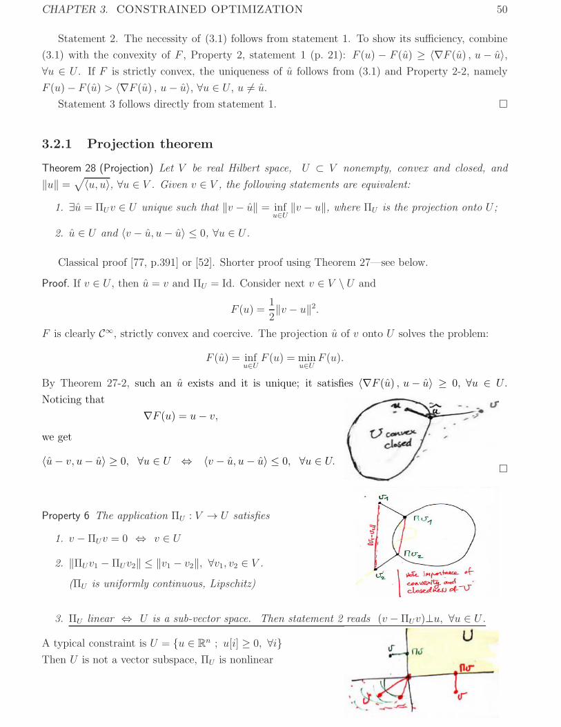
CHAPTER 3. CONSTRAINED OPTIMIZATION 50
Statement 2. The necessity of (3.1) follows from statement 1. To show its sufficiency, combine
(3.1) with the convexity of F , Property 2, statement 1 (p. 21): F (u) − F (u) ≥ 〈∇F (u) , u− u〉,∀u ∈ U . If F is strictly convex, the uniqueness of u follows from (3.1) and Property 2-2, namely
F (u)− F (u) > 〈∇F (u) , u− u〉, ∀u ∈ U , u �= u.
Statement 3 follows directly from statement 1. �
3.2.1 Projection theorem
Theorem 28 (Projection) Let V be real Hilbert space, U ⊂ V nonempty, convex and closed, and
‖u‖ = √〈u, u〉, ∀u ∈ V . Given v ∈ V , the following statements are equivalent:
1. ∃u = ΠUv ∈ U unique such that ‖v − u‖ = infu∈U‖v − u‖, where ΠU is the projection onto U ;
2. u ∈ U and 〈v − u, u− u〉 ≤ 0, ∀u ∈ U .
Classical proof [77, p.391] or [52]. Shorter proof using Theorem 27—see below.
Proof. If v ∈ U , then u = v and ΠU = Id. Consider next v ∈ V \ U and
F (u) =1
2‖v − u‖2.
F is clearly C∞, strictly convex and coercive. The projection u of v onto U solves the problem:
F (u) = infu∈U
F (u) = minu∈U
F (u).
By Theorem 27-2, such an u exists and it is unique; it satisfies 〈∇F (u) , u− u〉 ≥ 0, ∀u ∈ U .
Noticing that
∇F (u) = u− v,we get
〈u− v, u− u〉 ≥ 0, ∀u ∈ U ⇔ 〈v − u, u− u〉 ≤ 0, ∀u ∈ U. �
Property 6 The application ΠU : V → U satisfies
1. v − ΠUv = 0 ⇔ v ∈ U
2. ‖ΠUv1 − ΠUv2‖ ≤ ‖v1 − v2‖, ∀v1, v2 ∈ V .
(ΠU is uniformly continuous, Lipschitz)
3. ΠU linear ⇔ U is a sub-vector space. Then statement 2 reads (v − ΠUv)⊥u, ∀u ∈ U .
A typical constraint is U = {u ∈ Rn ; u[i] ≥ 0, ∀i}
Then U is not a vector subspace, ΠU is nonlinear
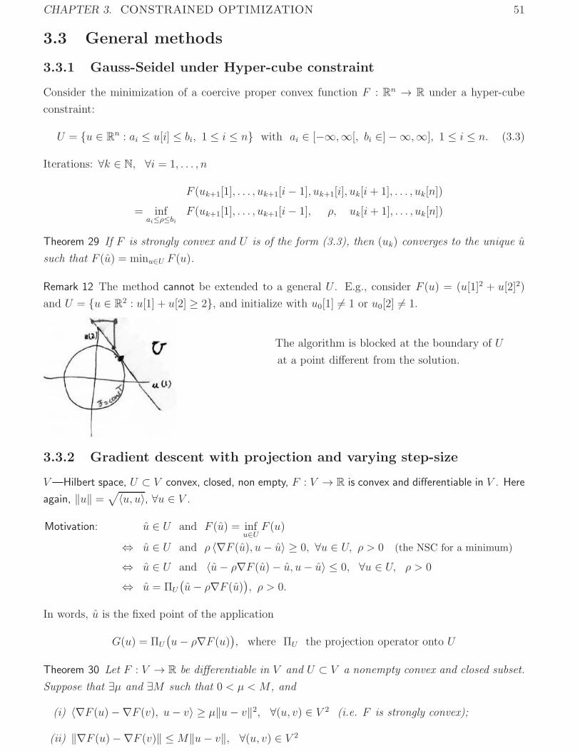
CHAPTER 3. CONSTRAINED OPTIMIZATION 51
3.3 General methods
3.3.1 Gauss-Seidel under Hyper-cube constraint
Consider the minimization of a coercive proper convex function F : Rn → R under a hyper-cube
constraint:
U = {u ∈ Rn : ai ≤ u[i] ≤ bi, 1 ≤ i ≤ n} with ai ∈ [−∞,∞[, bi ∈]−∞,∞], 1 ≤ i ≤ n. (3.3)
Iterations: ∀k ∈ N, ∀i = 1, . . . , n
F (uk+1[1], . . . , uk+1[i− 1], uk+1[i], uk[i+ 1], . . . , uk[n])
= infai≤ρ≤bi
F (uk+1[1], . . . , uk+1[i− 1], ρ, uk[i+ 1], . . . , uk[n])
Theorem 29 If F is strongly convex and U is of the form (3.3), then (uk) converges to the unique u
such that F (u) = minu∈U F (u).
Remark 12 The method cannot be extended to a general U . E.g., consider F (u) = (u[1]2 + u[2]2)
and U = {u ∈ R2 : u[1] + u[2] ≥ 2}, and initialize with u0[1] �= 1 or u0[2] �= 1.
The algorithm is blocked at the boundary of U
at a point different from the solution.
3.3.2 Gradient descent with projection and varying step-size
V—Hilbert space, U ⊂ V convex, closed, non empty, F : V → R is convex and differentiable in V . Here
again, ‖u‖ = √〈u, u〉, ∀u ∈ V .Motivation: u ∈ U and F (u) = inf
u∈UF (u)
⇔ u ∈ U and ρ 〈∇F (u), u− u〉 ≥ 0, ∀u ∈ U, ρ > 0 (the NSC for a minimum)
⇔ u ∈ U and 〈u− ρ∇F (u)− u, u− u〉 ≤ 0, ∀u ∈ U, ρ > 0
⇔ u = ΠU
(u− ρ∇F (u)), ρ > 0.
In words, u is the fixed point of the application
G(u) = ΠU
(u− ρ∇F (u)), where ΠU the projection operator onto U
Theorem 30 Let F : V → R be differentiable in V and U ⊂ V a nonempty convex and closed subset.
Suppose that ∃μ and ∃M such that 0 < μ < M , and
(i) 〈∇F (u)−∇F (v), u− v〉 ≥ μ‖u− v‖2, ∀(u, v) ∈ V 2 (i.e. F is strongly convex);
(ii) ‖∇F (u)−∇F (v)‖ ≤M‖u− v‖, ∀(u, v) ∈ V 2
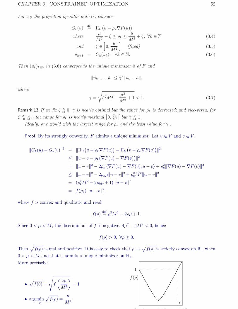
CHAPTER 3. CONSTRAINED OPTIMIZATION 52
For ΠU the projection operator onto U , consider
Gk(u)def= ΠU
(u− ρk∇F (u)
)where
μ
M2− ζ ≤ ρk ≤ μ
M2+ ζ, ∀k ∈ N (3.4)
and ζ ∈]0,
μ
M2
[(fixed) (3.5)
uk+1 = Gk(uk), ∀k ∈ N. (3.6)
Then (uk)k∈N in (3.6) converges to the unique minimizer u of F and
‖uk+1 − u‖ ≤ γk‖u0 − u‖,
where
γ =
√ζ2M2 − μ2
M2+ 1 < 1. (3.7)
Remark 13 If we fix ζ � 0, γ is nearly optimal but the range for ρk is decreased; and vice-versa, for
ζ � μM2 , the range for ρk is nearly maximal
]0, 2μ
M2
[but γ � 1.
Ideally, one would wish the largest range for ρk and the least value for γ...
Proof. By its strongly convexity, F admits a unique minimizer. Let u ∈ V and v ∈ V .
‖Gk(u)−Gk(v)‖2 = ‖ΠU
(u− ρk∇F (u)
)−ΠU
(v − ρk∇F (v)
)‖2≤ ‖u− v − ρk
(∇F (u)−∇F (v))‖2= ‖u− v‖2 − 2ρk 〈∇F (u)−∇F (v), u− v〉+ ρ2k‖∇F (u)−∇F (v)‖2≤ ‖u− v‖2 − 2ρkμ‖u− v‖2 + ρ2kM
2‖u− v‖2= (ρ2kM
2 − 2ρkμ+ 1) ‖u− v‖2= f(ρk) ‖u− v‖2,
where f is convex and quadratic and read
f(ρ)def= ρ2M2 − 2ρμ+ 1.
Since 0 < μ < M , the discriminant of f is negative, 4μ2 − 4M2 < 0, hence
f(ρ) > 0, ∀ρ ≥ 0.
Then√f(ρ) is real and positive. It is easy to check that ρ→√
f(ρ) is strictly convex on R+ when
0 < μ < M and that it admits a unique minimizer on R+.
More precisely:
f(ρ)
2 /M2/M2(0 0)
1 √f(ρ)
ρ
•√f(0) =
√f
(2μ
M2
)= 1
• argminρ
√f(ρ) =
μ
M2
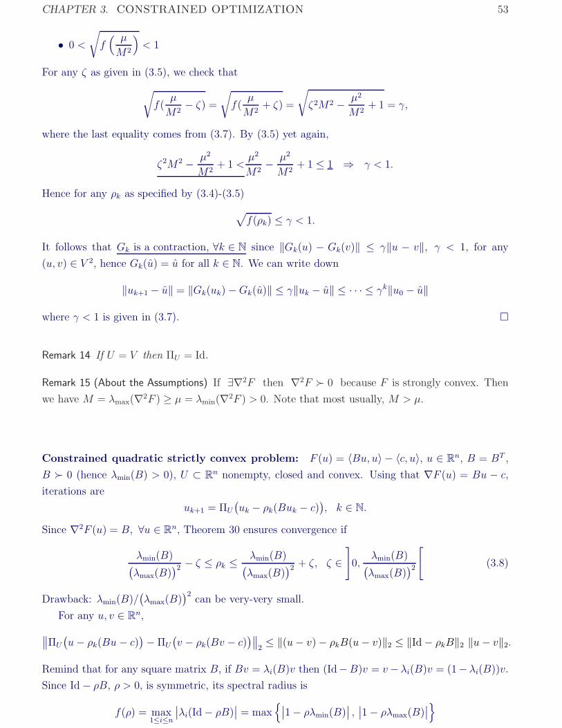
CHAPTER 3. CONSTRAINED OPTIMIZATION 53
• 0 <
√f( μ
M2
)< 1
For any ζ as given in (3.5), we check that√f(
μ
M2− ζ) =
√f(
μ
M2+ ζ) =
√ζ2M2 − μ2
M2+ 1 = γ,
where the last equality comes from (3.7). By (3.5) yet again,
ζ2M2 − μ2
M2+ 1 <
μ2
M2− μ2
M2+ 1 ≤ 1 ⇒ γ < 1.
Hence for any ρk as specified by (3.4)-(3.5)√f(ρk) ≤ γ < 1.
It follows that Gk is a contraction, ∀k ∈ N since ‖Gk(u) − Gk(v)‖ ≤ γ‖u − v‖, γ < 1, for any
(u, v) ∈ V 2, hence Gk(u) = u for all k ∈ N. We can write down
‖uk+1 − u‖ = ‖Gk(uk)−Gk(u)‖ ≤ γ‖uk − u‖ ≤ · · · ≤ γk‖u0 − u‖
where γ < 1 is given in (3.7). �
Remark 14 If U = V then ΠU = Id.
Remark 15 (About the Assumptions) If ∃∇2F then ∇2F � 0 because F is strongly convex. Then
we have M = λmax(∇2F ) ≥ μ = λmin(∇2F ) > 0. Note that most usually, M > μ.
Constrained quadratic strictly convex problem: F (u) = 〈Bu, u〉 − 〈c, u〉, u ∈ Rn, B = BT ,
B � 0 (hence λmin(B) > 0), U ⊂ Rn nonempty, closed and convex. Using that ∇F (u) = Bu − c,
iterations are
uk+1 = ΠU
(uk − ρk(Buk − c)
), k ∈ N.
Since ∇2F (u) = B, ∀u ∈ Rn, Theorem 30 ensures convergence if
λmin(B)(λmax(B)
)2 − ζ ≤ ρk ≤ λmin(B)(λmax(B)
)2 + ζ, ζ ∈]0,
λmin(B)(λmax(B)
)2[
(3.8)
Drawback: λmin(B)/(λmax(B)
)2can be very-very small.
For any u, v ∈ Rn,∥∥ΠU
(u− ρk(Bu− c)
)− ΠU
(v − ρk(Bv − c)
)∥∥2≤ ‖(u− v)− ρkB(u− v)‖2 ≤ ‖Id− ρkB‖2 ‖u− v‖2.
Remind that for any square matrix B, if Bv = λi(B)v then (Id−B)v = v− λi(B)v = (1− λi(B))v.
Since Id− ρB, ρ > 0, is symmetric, its spectral radius is
f(ρ) = max1≤i≤n
∣∣λi(Id− ρB)∣∣ = max
{∣∣1− ρλmin(B)∣∣ , ∣∣1− ρλmax(B)
∣∣}
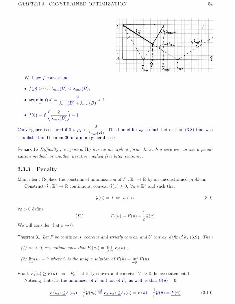
CHAPTER 3. CONSTRAINED OPTIMIZATION 54
We have f convex and
• f(ρ) > 0 if λmin(B) < λmax(B);
• argminρf(ρ) =
2
λmin(B) + λmax(B)< 1
• f(0) = f
(2
λmax(B)
)= 1
Convergence is ensured if 0 < ρk <2
λmax(B). This bound for ρk is much better than (3.8) that was
established in Theorem 30 in a more general case.
Remark 16 Difficulty : in general ΠU has no an explicit form. In such a case we can use a penal-
ization method, or another iterative method (see later sections).
3.3.3 Penalty
Main idea : Replace the constrained minimization of F : Rn → R by an unconstrained problem.
Construct G : Rn → R continuous, convex, G(u) ≥ 0, ∀u ∈ Rn and such that
G(u) = 0 ⇔ u ∈ U (3.9)
∀ε > 0 define
(Pε) Fε(u) = F (u) +1
εG(u)
We will consider that ε→ 0.
Theorem 31 Let F be continuous, coercive and strictly convex, and U convex, defined by (3.9). Then
(1) ∀ε > 0, ∃uε unique such that Fε(uε) = infu∈Rn
Fε(u) ;
(2) limε→0
uε = u where u is the unique solution of F (u) = infu∈U
F (u).
Proof. Fε(u) ≥ F (u) ⇒ Fε is strictly convex and coercive, ∀ε > 0, hence statement 1.
Noticing that u is the minimizer of F and not of Fε, as well as that G(u) = 0,
F (uε) ≤F (uε) + 1
εG(uε) def
= Fε(uε) ≤Fε(u) = F (u) +1
εG(u) = F (u) (3.10)
CHAPTER 3. CONSTRAINED OPTIMIZATION 55
Since Fε is coercive, (uε)ε>0 is bounded. Hence there is a convergent subsequence (uεk)k∈N, say
limk→∞
uεk = u (3.11)
Using (3.10)
F (uεk) ≤ Fεk(uεk) ≤ F (u) (3.12)
Since F is continuous,
F (u) = limk→∞
F (uεk)≤ F (u) (3.13)
By the expression for (Pε) and (3.12),
0 ≤ G(uεk) = εk(Fεk(uεk)− F (uεk)
) ≤ εk(F (u)− F (uεk)
) ≤ εkK,
where K is un upper bound for F (u) − F (uεk), independent of k. By the continuity of G, (3.11)yields
limk→∞G(uεk) = G(u),
and reminding that εk → 0 as k →∞,
limk→∞G(uεk) ≤ lim
k→∞εkK = 0
The last two results show that G(u) = 0, hence u ∈ U . Using (3.13) and the fact that F has a
unique minimizer in U show that
u = u ⇒ limε→0
uε = u.
The proof is complete. �
Convex programming Problem : U given by (1.2), i.e.
U = {u ∈ Rn | hi(u) ≤ 0, 1 ≤ i ≤ q}
with hi : Rn → R, i = 1, . . . , q convex functions. Consider
G(u) =
q∑i=1
gi(u),
gi(u) = max{hi(u), 0}
G clearly satisfies the requirements for continuity, convexity and (3.9). Let us check the last point
(3.9). If for all 1 ≤ i ≤ q we have hi(u) ≤ 0, i.e. u ∈ U , then gi(u) = 0 for all 1 ≤ i ≤ q and thus
G(u) = 0. Note that G(u) � 0 for all u ∈ Rn. If u �∈ U , there is at least one index i such that
hi(u) > 0 which leads to gi(u) > 0 and G(u) > 0. Thus G(u) = 0 shows that u ∈ U .
Comments Note that G is not necessarily differentiable.
Difficulty : construct “good” functions G (differentiable, convex). This constitutes the main
limitation of penalization methods.
CHAPTER 3. CONSTRAINED OPTIMIZATION 56
3.4 Equality constraints
3.4.1 Lagrange multipliers
Here V1, V2 and Y are n.v.s. Optimality conditions are based on the Implicit functions theorem.
Theorem 32 (Implicit functions theorem) Let G : O ⊂ V1 × V2 → Y be C1 in O, where V2 and Y are
complete (i.e. Banach spaces). Suppose that u = (u1, u2) ∈ O and v ∈ Y are such that G(u1, u2) = v
and D2 G(u1, u2) ∈ Isom(V2 ; Y ).
Then ∃O1 ⊂ V1, ∃O2 ⊂ V2 such that (u1, u2) ∈ O1 × O2 ⊂ O and there is a unique continuous
function g : O1 ⊂ V1 → V2, called an implicit function, such that
{(u1, u2) ∈ O1 ×O2 : G(u1, u2) = v} = {( u1, u2) ∈ O1 × V2 : u2 = g(u1)}.
Moreover g is differentiable at u1 and
Dg(u1) = − (D2G(u1, u2))−1D1G(u1, u2). (3.14)
Proof. See [11, p. 30], [78, p. 176]
As to differentiability (note that g is differentiable at u1):
G(u1, g(u1))− v = 0 ∈ Y, ∀u1 ∈ O1.
Differentiation of both sides of this identity w.r.t. u1 = u1 yields
D1G(u1, g(u1)) +D2G(u1, g(u1))Dg(u1) = 0.
Hence (3.14).
Example 5 V1 = V2 = R, G(u1, u2) = u21 − u2 = 0 = v ∈ Y = R. Then D2G(u) = −1 ∈ Isom(R,R)
and u2 = g(u1) = u21. Thus G(u1, u2) = 0 = G(u1, g(u1)), ∀u1 ∈ R.
Theorem 33 (Necessary condition for a constrained minimum) Let O ⊂ V = V1 × V2 be open where V1
and V2 are real n.v.s., and V2 be complete. Consider that G : O → V2 is C1 and set
U = {u ∈ O : G(u1, u2) = 0}.
Suppose that F : V → R is differentiable at u ∈ U and that D2G(u) ∈ Isom(V2, V2). If F has a
relative minimum w.r.t. U at u, then there is an application λ(u) ∈ L(V2,R) such that
DF (u) + λ(u)DG(u) = 0. (3.15)
CHAPTER 3. CONSTRAINED OPTIMIZATION 57
Proof. By the Implicit Functions Theorem 32, there are two open sets O1 ∈ V1 and O2 ∈ V2, withu ∈ O1 ×O2 ⊂ O, and a continuous application g : O1 → O2 such that
(O1 ×O2) ∩ U = {(u1, u2) ∈ (O1 × V2) | u2 = g(u1)}
and
Dg(u1) = −(D2G(u))−1D1G(u). (3.16)
Define
F(u1) def= F
(u1, g(u1)
), ∀u1 ∈ O1.
Then F(u1) = infu1∈O1
F(u1) entails F (u) = infu∈U
F (u) for u =(u1, g(u1)
). Since O1 is open, u1 satisfies
0 = DF(u1) = D1F(u1, g(u1)
)+D2F
(u1, g(u1)
)Dg(u1)
= D1F(u1, g(u1)
)−D2F(u1, g(u1)
)(D2G(u))−1D1G(u),
where the last equality comes from (3.16). Using that u =(u1, g(u1)
), we can hence write down
D1F (u) = D2F (u) (D2G(u))−1D1G(u)D2F (u) = D2F (u) (D2G(u))−1D2G(u)
where the second equality is just an identity. We obtain (3.15) by setting
λ(u) = −D2F (u) (D2G(u))−1.
Since D2F (u) ∈ L(V2 ;R) and (D2G(u))−1 ∈ L(V2 ;V2), we have λ(u) ∈ L(V2 ;R). �
The most usual case arising in practice is considered in the next theorem.
Theorem 34 Let O ⊂ Rn be open and gi : O → R, 1 ≤ i ≤ p be C1-functions in O.
U = {u ∈ O : gi(u) = 0, 1 ≤ i ≤ p} ⊂ O
Let Dgi(u) ∈ L(Rn,R), 1 ≤ i ≤ p be linearly independent and F : O → R differentiable at u. If
u ∈ U solves the problem infu∈U
F (u) then there exist p real numbers λi(u) ∈ R, 1 ≤ i ≤ p, uniquely
defined, such that
DF (u) +
p∑i=1
λi(u) Dgi(u) = 0. (3.17)
λi(u), 1 ≤ i ≤ p are called the Lagrange multipliers.
The problem considered in the last theorem is a particular case of Theorem 33.
Proof. Put G def= (g1, · · · , gp). Then
DG(u) =⎡⎣ Dg1(u)
· · ·Dgp(u)
⎤⎦ =
⎡⎢⎣∂g1∂u1
· · · ∂g1∂up
· · · ∂g1∂un
· · ·∂gp∂u1
· · · ∂gp∂up
· · · ∂gp∂un
⎤⎥⎦
CHAPTER 3. CONSTRAINED OPTIMIZATION 58
Since Dgi(u) are linearly independent, rank(DG(u)) = p ≤ n, so we can assume that the first p× psubmatrix of DG(u) is invertible. If p = n, u is uniquely determined by G. Consider next that p < n.
Let {e1, · · · en} be the canonical basis of Rn. Define
V1def= Span{ep+1, · · · , en}
V2def= Span{e1, · · · , ep}
Redefine G in the following way:
G : V1 × V2 → V2
(u1, u2) → G(u) =p∑
i=1
gi(u)ei.
Since the first p × p submatrix of DG(u) is invertible, D2G(u) ∈ Isom(V2, V2). Noticing that the
elements of V2 belong to Rp, Theorem 33 shows that there exists λ(u) ∈ R
p (i.e. real numbers λi(u),
1 ≤ i ≤ p) such that
DF (u) + λ(u)DG(u) = 0 ⇔ DF (u) +
p∑i=1
λi(u)Dgi(u) = 0
The uniqueness of λ(u) is due to the fact that rank(DG(u)) = p. �
Remark 17 Since F : O ∈ Rn → R and gi : O ∈ R
n → R, 1 ≤ i ≤ p, we can identify differentials
with gradients using the scalar product on R�, � ∈ {p, n}. Then (3.17) can be rewritten as
∇F (u) +p∑
i=1
λi(u) ∇gi(u) = 0. (3.18)
The numbers λi(u), i ∈ {1, 2, · · · , p} are called Lagrange multipliers relevant to a constraint
extremum (minimum or maximum) of F in U .
To resume: u ∈ Rn, λ ∈ R
p hence n+ p unknowns{ ∇F (u) +∑pi=1 λi∇gi(u) = 0 n equations
gi(u) = 0, 1 ≤ i ≤ p p equations
System of n+ p (nonlinear) equations.
These are necessary conditions. Complete the resolution of the problem by analyzing if u indeed
is a minimizer. In particular, if F is convex and continuous, and if U is convex and {∇gi} linearlyindependent on V , then (3.18) yields the minimum of F .
3.4.2 Application to linear systems
Quadratic function under affine constraints
For B ∈ Rn×n, B = BT , B � 0, and c ∈ R
n, consider
minimize F (u) =1
2〈Bu, u〉 − 〈c, u〉 subject to u ∈ U
where U = {u ∈ Rn : Au = v} with A ∈ R
p×n, rankA = p < n. (3.19)
(3.18) yieldsBu+ ATλ = c
Au = v(3.20)

CHAPTER 3. CONSTRAINED OPTIMIZATION 59
Projection onto U in (3.19) The projection u = ΠU(w) of w ∈ (Rn \ U) onto U satisfies
u = argminu∈U
1
2‖u− w‖2 = argmin
u∈U
(1
2〈u, u〉 − 〈w, u〉
).
(3.20) yieldsu+ ATλ = wAu = v
Hence
Au+ AATλ = Aw ⇒ λ = (AAT )−1A(w − u) = (AAT )−1(Aw − v)Since AAT is invertible (see (3.19)), we get
u+ ATλ = u+ AT (AAT )−1(Aw − v) = w
We deduce
u = ΠU(w) =(I − AT (AAT )−1A
)w + AT (AAT )−1v (3.21)
• If p = 1, then A ∈ R1×n is a row-vector, v ∈ R and AAT = ‖A‖22.
• If v = 0, then U = kerA is a vector sub-space and ΠU is linear
ΠU = I −AT (AAT )−1A (3.22)
“Solving” a linear system: Au = v ∈ Rm where u ∈ R
n
• rankA = m ≤ n : F (u) = ‖u‖2, U = {u ∈ Rn : Au = v}
u = AT (AAT )−1v (the minimum norm solution). Compare with (3.22).
• rankA = n ≤ m : F (u) = ‖Au− v‖2, U = Rn
u = (ATA)−1ATv (the least-squares (LS) solution)
Generalized inverse, pseudoinverse — if A has linearly dependent rows or columns
SVD (singular value decomposition) of A ∈ Rm×n :
A = Q1ΣQ2
• Q1QT1 = QT
1Q1 = Im, Q2QT2 = QT
2Q2 = In (orthonormal matrices)
• the columns of Q1 = eigenvectors of AAT
• the columns of Q2 = eigenvectors of de ATA
• Σ, m × n, diagonal, Σ[i, i], 1 ≤ i ≤ r singular values =√eigenvalues �= 0 of AAT and ATA,
r = rankA
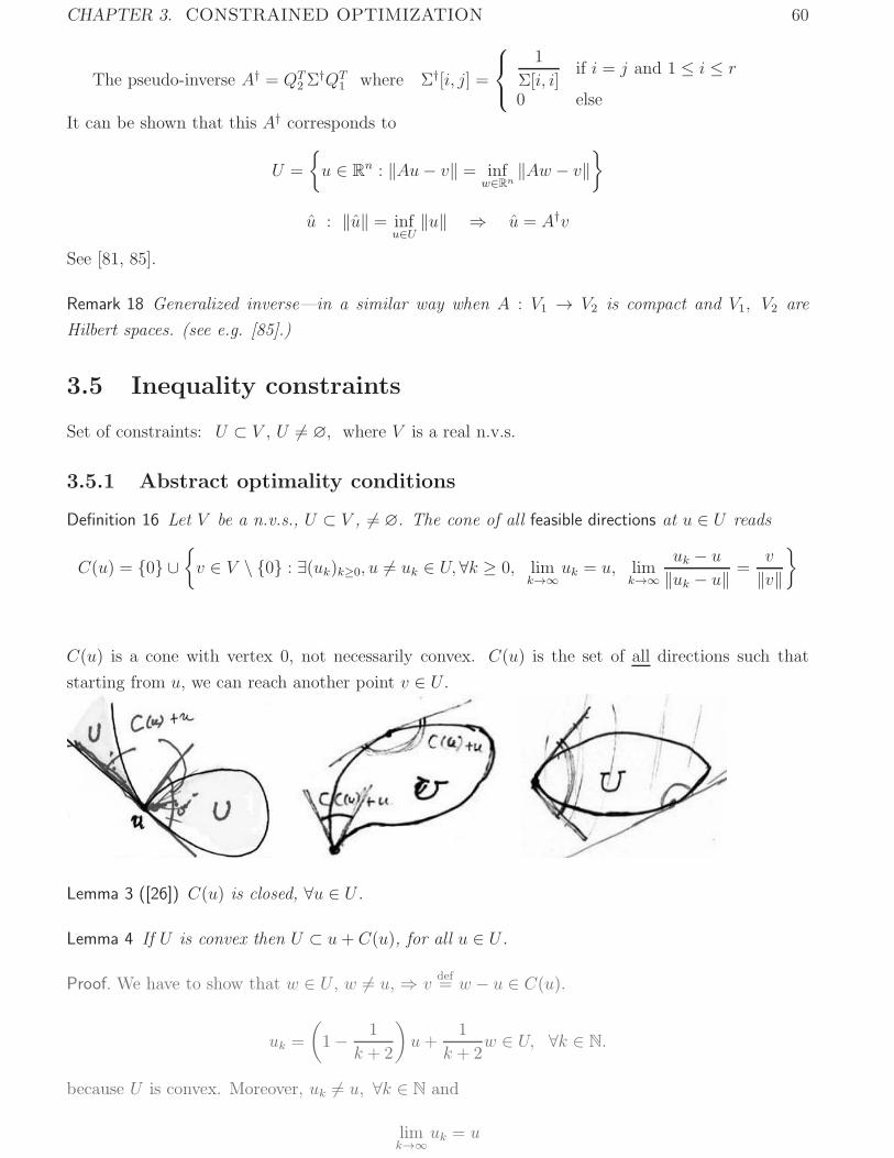
CHAPTER 3. CONSTRAINED OPTIMIZATION 60
The pseudo-inverse A† = QT2Σ
†QT1 where Σ†[i, j] =
⎧⎨⎩1
Σ[i, i]if i = j and 1 ≤ i ≤ r
0 else
It can be shown that this A† corresponds to
U =
{u ∈ R
n : ‖Au− v‖ = infw∈Rn
‖Aw − v‖}
u : ‖u‖ = infu∈U‖u‖ ⇒ u = A†v
See [81, 85].
Remark 18 Generalized inverse—in a similar way when A : V1 → V2 is compact and V1, V2 are
Hilbert spaces. (see e.g. [85].)
3.5 Inequality constraints
Set of constraints: U ⊂ V , U �= ∅, where V is a real n.v.s.
3.5.1 Abstract optimality conditions
Definition 16 Let V be a n.v.s., U ⊂ V , �= ∅. The cone of all feasible directions at u ∈ U reads
C(u) = {0} ∪{v ∈ V \ {0} : ∃(uk)k≥0, u �= uk ∈ U, ∀k ≥ 0, lim
k→∞uk = u, lim
k→∞uk − u‖uk − u‖ =
v
‖v‖}
C(u) is a cone with vertex 0, not necessarily convex. C(u) is the set of all directions such that
starting from u, we can reach another point v ∈ U .
Lemma 3 ([26]) C(u) is closed, ∀u ∈ U .
Lemma 4 If U is convex then U ⊂ u+ C(u), for all u ∈ U .
Proof. We have to show that w ∈ U , w �= u, ⇒ vdef= w − u ∈ C(u).
uk =
(1− 1
k + 2
)u+
1
k + 2w ∈ U, ∀k ∈ N.
because U is convex. Moreover, uk �= u, ∀k ∈ N and
limk→∞
uk = u
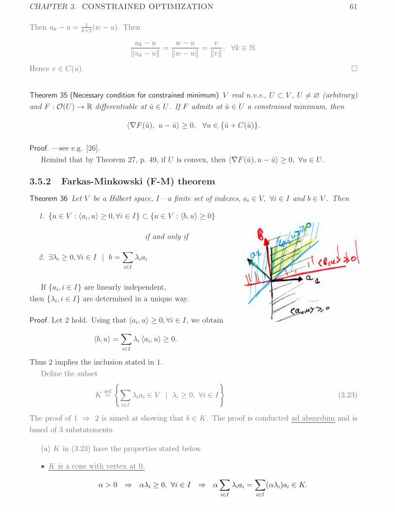
CHAPTER 3. CONSTRAINED OPTIMIZATION 61
Then uk − u = 1k+2
(w − u). Thenuk − u‖uk − u‖ =
w − u‖w − u‖ =
v
‖v‖ , ∀k ∈ N.
Hence v ∈ C(u). �
Theorem 35 (Necessary condition for constrained minimum) V real n.v.s., U ⊂ V , U �= ∅ (arbitrary)
and F : O(U)→ R differentiable at u ∈ U . If F admits at u ∈ U a constrained minimum, then
〈∇F (u), u− u〉 ≥ 0, ∀u ∈ {u+ C(u)}.
Proof. —see e.g. [26].
Remind that by Theorem 27, p. 49, if U is convex, then 〈∇F (u), u− u〉 ≥ 0, ∀u ∈ U .
3.5.2 Farkas-Minkowski (F-M) theorem
Theorem 36 Let V be a Hilbert space, I—a finite set of indexes, ai ∈ V, ∀i ∈ I and b ∈ V . Then
1. {u ∈ V : 〈ai, u〉 ≥ 0, ∀i ∈ I} ⊂ {u ∈ V : 〈b, u〉 ≥ 0}
if and only if
2. ∃λi ≥ 0, ∀i ∈ I | b =∑i∈I
λiai
If {ai, i ∈ I} are linearly independent,
then {λi, i ∈ I} are determined in a unique way.
Proof. Let 2 hold. Using that 〈ai, u〉 ≥ 0, ∀i ∈ I, we obtain
〈b, u〉 =∑i∈I
λi 〈ai, u〉 ≥ 0.
Thus 2 implies the inclusion stated in 1.
Define the subset
Kdef=
{∑i∈I
λiai ∈ V | λi ≥ 0, ∀i ∈ I}
(3.23)
The proof of 1 ⇒ 2 is aimed at showing that b ∈ K. The proof is conducted ad absurdum and is
based of 3 substatements.
(a) K in (3.23) have the properties stated below.
• K is a cone with vertex at 0.
α > 0 ⇒ αλi ≥ 0, ∀i ∈ I ⇒ α∑i∈I
λiai =∑i∈I
(αλi)ai ∈ K.

CHAPTER 3. CONSTRAINED OPTIMIZATION 62
• K is convex.
Let 0 < θ < 1, λi ≥ 0, ∀i ∈ I and μi ≥ 0, ∀i ∈ I.
θ∑i∈I
λiai + (1− θ)∑i∈I
μiai =∑i∈I
(θλi + (1− θ)μi
)ai ∈ K
because θλi + (1− θ)μi ≥ 0.
• K is closed in V .
– Suppose that {ai, i ∈ I} are linearly independent. Set A = Span{ai : i ∈ I}—a finite
dimensional vector subspace (hence closed). Consider an arbitrary (vj)j∈N ⊂ K. For any
j ∈ N, there is a unique set {λj[i] ≥ 0, i ∈ I} so that
vj =∑i∈I
λj[i]ai ∈ K ∩ A.
Let limj→∞
vj = v ∈ V then v ∈ V ∩A which is equivalent to
limj→∞
vj =∑i∈I
(limj→∞
λj[i]
)ai ∈ K ∩A.
Hence K is closed in V .
– Let {ai, i ∈ I} be linearly dependent. Then K is a finite union of cones corresponding
to linearly independent subsets of {ai}. These cones are closed, hence K is closed.
(b) Let K ⊂ V be convex, closed and K �= ∅. Let b ∈ V \ K. Using the Hahn-Banach theorem 3,
∃h ∈ V and ∃α ∈ R such that
〈u, h〉 > α, ∀u ∈ K,〈b, h〉 < α.
By the Projection Theorem 28 (p. 50), there is a unique c ∈ K such that
‖b− c‖ = infu∈K‖b− u‖ > 0 (> 0 because b �∈ K)
c ∈ V satisfies
〈u− c, b− c〉 ≤ 0, ∀u ∈ K. (3.24)
Then
‖c− b‖2 > 0 ⇔ ‖c‖2 − 〈c, b〉 − 〈c, b〉+ ‖b‖2 > 0
⇔ ‖c‖2 − 〈c, b〉 > 〈c, b〉 − ‖b‖2 ⇔ 〈c, c− b〉 > 〈b, c− b〉
Set h = c− b and α such that
〈c, c− b〉 = 〈c, h〉 > α > 〈b, h〉 = 〈b, c− b〉
From (3.24)
〈u− c, h〉 ≥ 0 ⇒ 〈u, h〉 ≥ 〈c, h〉> α, ∀u ∈ K.
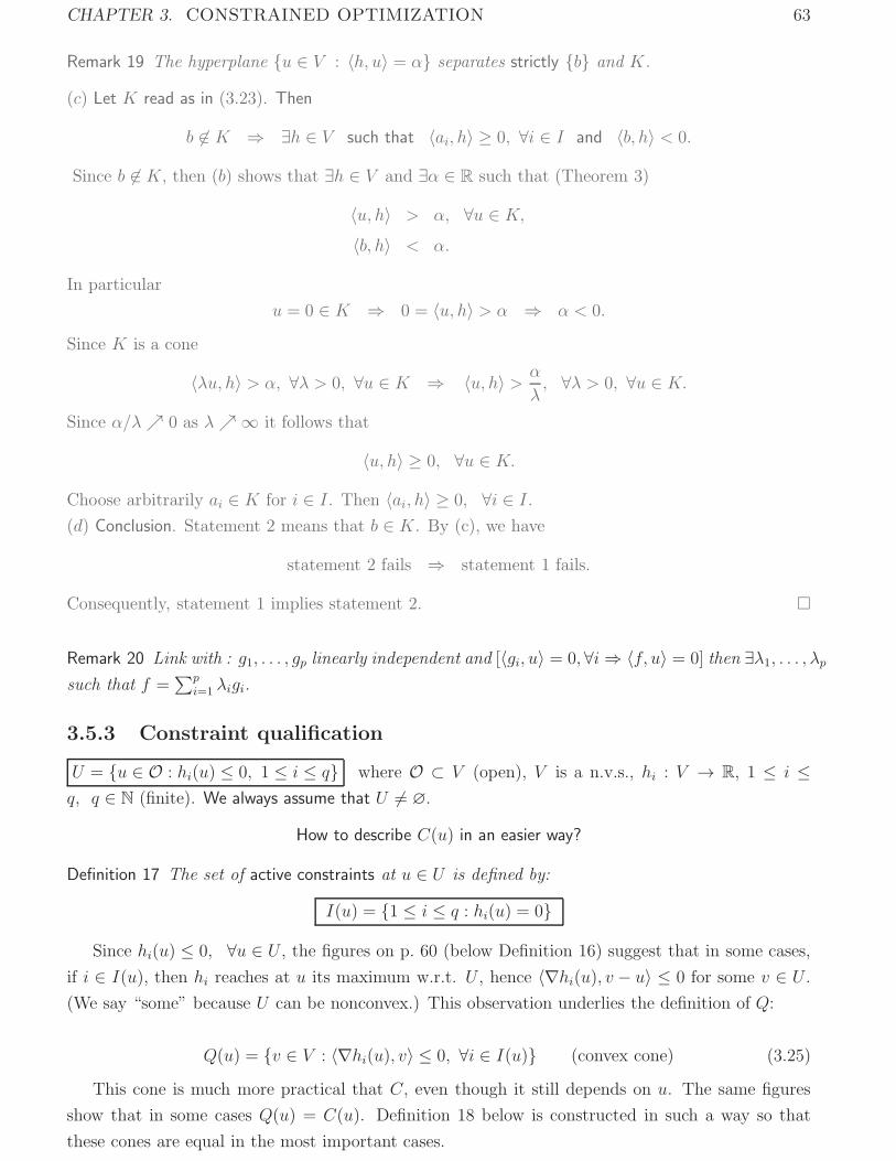
CHAPTER 3. CONSTRAINED OPTIMIZATION 63
Remark 19 The hyperplane {u ∈ V : 〈h, u〉 = α} separates strictly {b} and K.
(c) Let K read as in (3.23). Then
b �∈ K ⇒ ∃h ∈ V such that 〈ai, h〉 ≥ 0, ∀i ∈ I and 〈b, h〉 < 0.
Since b �∈ K, then (b) shows that ∃h ∈ V and ∃α ∈ R such that (Theorem 3)
〈u, h〉 > α, ∀u ∈ K,〈b, h〉 < α.
In particular
u = 0 ∈ K ⇒ 0 = 〈u, h〉 > α ⇒ α < 0.
Since K is a cone
〈λu, h〉 > α, ∀λ > 0, ∀u ∈ K ⇒ 〈u, h〉 > α
λ, ∀λ > 0, ∀u ∈ K.
Since α/λ↗ 0 as λ↗∞ it follows that
〈u, h〉 ≥ 0, ∀u ∈ K.
Choose arbitrarily ai ∈ K for i ∈ I. Then 〈ai, h〉 ≥ 0, ∀i ∈ I.(d) Conclusion. Statement 2 means that b ∈ K. By (c), we have
statement 2 fails ⇒ statement 1 fails.
Consequently, statement 1 implies statement 2. �
Remark 20 Link with : g1, . . . , gp linearly independent and [〈gi, u〉 = 0, ∀i⇒ 〈f, u〉 = 0] then ∃λ1, . . . , λpsuch that f =
∑pi=1 λigi.
3.5.3 Constraint qualification
U = {u ∈ O : hi(u) ≤ 0, 1 ≤ i ≤ q} where O ⊂ V (open), V is a n.v.s., hi : V → R, 1 ≤ i ≤q, q ∈ N (finite). We always assume that U �= ∅.
How to describe C(u) in an easier way?
Definition 17 The set of active constraints at u ∈ U is defined by:
I(u) = {1 ≤ i ≤ q : hi(u) = 0}
Since hi(u) ≤ 0, ∀u ∈ U , the figures on p. 60 (below Definition 16) suggest that in some cases,
if i ∈ I(u), then hi reaches at u its maximum w.r.t. U , hence 〈∇hi(u), v − u〉 ≤ 0 for some v ∈ U .(We say “some” because U can be nonconvex.) This observation underlies the definition of Q:
Q(u) = {v ∈ V : 〈∇hi(u), v〉 ≤ 0, ∀i ∈ I(u)} (convex cone) (3.25)
This cone is much more practical that C, even though it still depends on u. The same figures
show that in some cases Q(u) = C(u). Definition 18 below is constructed in such a way so that
these cones are equal in the most important cases.

CHAPTER 3. CONSTRAINED OPTIMIZATION 64
Definition 18 The constraints are qualified at u ∈ U if one of the following conditions hold:
• ∃w ∈ V \ {0} such that ∀i ∈ I(u), 〈∇hi(u), w〉 ≤ 0, where the inequality is strict if hi is
not affine;
• hi is affine, ∀i ∈ I(u).
Naturally, Q(u) = V if I(u) = ∅.
Lemma 5 ([26]) Let hi for i ∈ I(u) be differentiable at u ⇒ C(u) ⊂ Q(u)
Theorem 37 ([26]) Assume that
(i) hi differentiable at u, ∀i ∈ I(u)(ii) hi continuous at u, ∀i ∈ I \ I(u)(iii) Constraints are qualified at u
⇒ C(u) = Q(u)
Example 6 U = {v ∈ Rn : 〈ai, v〉 ≤ bi, 1 ≤ i ≤ q} �= ∅ (then the constraints are qualified ∀v ∈ U)
and we have C(u) = Q(u) = {v ∈ Rn : 〈ai, v〉 ≤ 0, ∀i ∈ I(u)}
3.5.4 Kuhn & Tucker Relations
Putting together all previous results leads to one of the most important statements in Optimization
theorey—the Kuhn-Tucker (KT) relations, stated below.
Theorem 38 (Necessary conditions for a minimum) V—Hilbert space, O ⊂ V open, hi : O → R, ∀i
U = {u ∈ O : hi(u) ≤ 0, 1 ≤ i ≤ q} (3.26)
(i) hi differentiable at u, ∀i ∈ I(u)(ii) hi continuous at u, ∀i ∈ I \ I(u)(iii) Constraints are qualified at u ∈ U(iv) F : O → R differentiable at u(v) F has a relative minimum at u w.r.t. U
Then
∃λi(u) ≥ 0, 1 ≤ i ≤ q such that ∇F (u) +q∑
i=1
λi(u)∇hi(u) = 0,
q∑i=1
λi(u)hi(u) = 0 . (3.27)
λi(u) are called Generalized Lagrange Multipliers
Proof. Assumptions (i), (ii) and (iii) are as in Theorem 37, hence
C(u) = Q(u).
By Theorem 35 (p. 61), or equivalently by Theorem 27 (p. 49)—since Q(u) is convex,
〈∇F (u), v〉 ≥ 0, ∀v def= u− u ∈ Q(u) . (3.28)
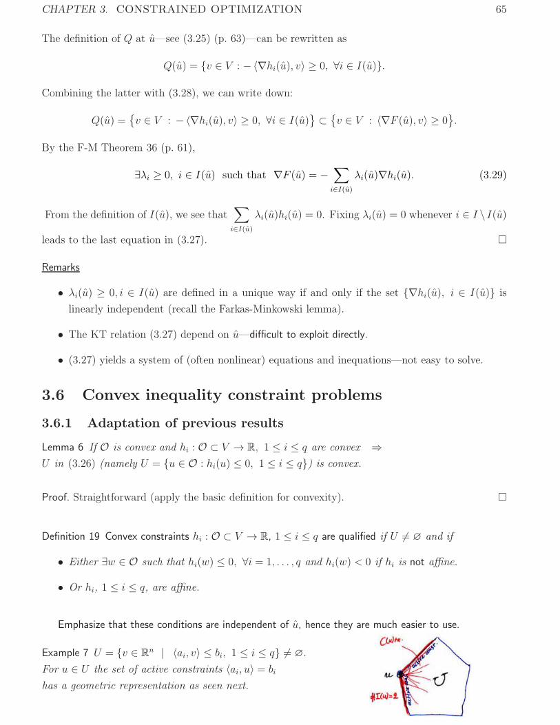
CHAPTER 3. CONSTRAINED OPTIMIZATION 65
The definition of Q at u—see (3.25) (p. 63)—can be rewritten as
Q(u) = {v ∈ V : −〈∇hi(u), v〉 ≥ 0, ∀i ∈ I(u)}.
Combining the latter with (3.28), we can write down:
Q(u) ={v ∈ V : −〈∇hi(u), v〉 ≥ 0, ∀i ∈ I(u)} ⊂ {
v ∈ V : 〈∇F (u), v〉 ≥ 0}.
By the F-M Theorem 36 (p. 61),
∃λi ≥ 0, i ∈ I(u) such that ∇F (u) = −∑i∈I(u)
λi(u)∇hi(u). (3.29)
From the definition of I(u), we see that∑i∈I(u)
λi(u)hi(u) = 0. Fixing λi(u) = 0 whenever i ∈ I \ I(u)
leads to the last equation in (3.27). �
Remarks
• λi(u) ≥ 0, i ∈ I(u) are defined in a unique way if and only if the set {∇hi(u), i ∈ I(u)} is
linearly independent (recall the Farkas-Minkowski lemma).
• The KT relation (3.27) depend on u—difficult to exploit directly.
• (3.27) yields a system of (often nonlinear) equations and inequations—not easy to solve.
3.6 Convex inequality constraint problems
3.6.1 Adaptation of previous results
Lemma 6 If O is convex and hi : O ⊂ V → R, 1 ≤ i ≤ q are convex ⇒U in (3.26) (namely U = {u ∈ O : hi(u) ≤ 0, 1 ≤ i ≤ q}) is convex.
Proof. Straightforward (apply the basic definition for convexity). �
Definition 19 Convex constraints hi : O ⊂ V → R, 1 ≤ i ≤ q are qualified if U �= ∅ and if
• Either ∃w ∈ O such that hi(w) ≤ 0, ∀i = 1, . . . , q and hi(w) < 0 if hi is not affine.
• Or hi, 1 ≤ i ≤ q, are affine.
Emphasize that these conditions are independent of u, hence they are much easier to use.
Example 7 U = {v ∈ Rn | 〈ai, v〉 ≤ bi, 1 ≤ i ≤ q} �= ∅.
For u ∈ U the set of active constraints 〈ai, u〉 = bi
has a geometric representation as seen next.
CHAPTER 3. CONSTRAINED OPTIMIZATION 66
Theorem 39 (Necessary and sufficient conditions for a minimum on U) Let V be a Hilbert space, O ⊂V (open) and U ⊃ O convex. Suppose u ∈ U and that
(i) F : O ⊂ V → R and hi : O ⊂ V → R, 1 ≤ i ≤ q are differentiable at u;
(ii) hi : V → R, 1 ≤ i ≤ q, are convex;
(iii) Convex constraints qualification holds (Definition 19).
Then we have the following statements:
1. If F admits at u ∈ U a relative minimum w.r.t. U , then
∃ {λi(u) ∈ R+ : 1 ≤ i ≤ q} such that
∇F (u) +q∑
i=1
λi(u)∇hi(u) = 0 and (3.30)
q∑i=1
λi(u)hi(u) = 0 . (3.31)
2. If F is convex on U and (3.30)-(3.31) holds then F has at u a constrained minimum w.r.t. U .
Proof. To prove 1, we have to show that if the constraints are qualified in the convex sense (Definition
19) then they are qualified in the general sense (Definition 18, p. 64), for any u ∈ U , which will
allows us to apply the KT Theorem 38.
• Let w �= u, w ∈ U , satisfy Definition 19. Set v = w − u. Using that hi(u) = 0, ∀i ∈ I(u), andthat hi are convex (see Property 2-1, p. 21),
i ∈ I(u) ⇒ 〈∇hi(u), v〉 = hi(u) + 〈∇hi(u), w − u〉 ≤ hi(w).
By Definition 19, we know that hi(w) ≤ 0 and that hi(w) < 0 is hi is not affine. Then
〈∇hi(u), w − u〉 = 〈∇hi(u), v〉 ≤ 0 ,
where the inequality is strict if hi is not affine. Hence Definition 18 is satisfied for v.
• Let u = w ∈ U . Since hi(u) < 0 is impossible for any i ∈ I(u), Definition 19 means that all hi
for i ∈ I(u) are affine. Then Definition 18 is trivially satisfied.
Statement 1 is a straightforward consequence of the KT relations (Theorem 38, p. 64).
To prove statement 2, we have to check that F (u) ≤ F (u), ∀u ∈ U . Let u ∈ U (arbitrary). The
convexity of hi (Property 2-1) and the definition of U yield the two inequalities below:
i ∈ I(u) ⇒ 〈∇hi(u), u− u〉 ≤ hi(u)− hi(u) ≤ 0, ∀u ∈ U.
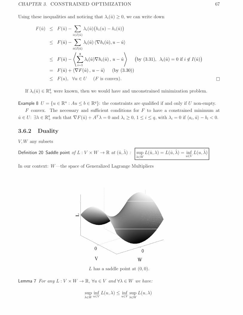
CHAPTER 3. CONSTRAINED OPTIMIZATION 67
Using these inequalities and noticing that λi(u) ≥ 0, we can write down
F (u) ≤ F (u)−∑i∈I(u)
λi(u)(hi(u)− hi(u)
)≤ F (u)−
∑i∈I(u)
λi(u) 〈∇hi(u), u− u〉
≤ F (u)−⟨
q∑i=1
λi(u)∇hi(u) , u− u⟩ (
by (3.31), λi(u) = 0 if i �∈ I(u))= F (u) + 〈∇F (u) , u− u〉 (by (3.30))
≤ F (u), ∀u ∈ U (F is convex). �
If λi(u) ∈ Rq+ were known, then we would have and unconstrained minimization problem.
Example 8 U = {u ∈ Rn : Au ≤ b ∈ R
q}: the constraints are qualified if and only if U non-empty.
F convex. The necessary and sufficient conditions for F to have a constrained minimum at
u ∈ U : ∃λ ∈ Rq+ such that ∇F (u) + ATλ = 0 and λi ≥ 0, 1 ≤ i ≤ q, with λi = 0 if 〈ai, u〉 − bi < 0.
3.6.2 Duality
V,W any subsets
Definition 20 Saddle point of L : V ×W → R at (u, λ) : supλ∈W
L(u, λ) = L(u, λ) = infu∈V
L(u, λ)
In our context: W—the space of Generalized Lagrange Multipliers
L has a saddle point at (0, 0).
Lemma 7 For any L : V ×W → R, ∀u ∈ V and ∀λ ∈ W we have:
supλ∈W
infu∈V
L(u, λ) ≤ infu∈V
supλ∈W
L(u, λ)
CHAPTER 3. CONSTRAINED OPTIMIZATION 68
Proof. Take u ∈ V , λ ∈ W arbitrary.
infu∈V
L(u, λ) ≤ L(u, λ) ≤ supλ∈W
L(u, λ), ∀u ∈ V
infu∈V
L(u, λ) ≤ infu∈V
supλ∈W
L(u, λ)def= K
infu∈V
L(u, λ) ≤ K, ∀λ ∈ W ⇒ supλ∈W
infu∈V
L(u, λ) ≤ K = infu∈V
supλ∈W
L(u, λ)
The proof is complete. �
Theorem 40 Let (u, λ) be a saddle-point for L : V ×W → R. Then
supλ∈W
infu∈V
L(u, λ) = L(u, λ) = infu∈V
supλ∈W
L(u, λ).
Proof.
infu∈V
(supλ∈W
L(u, λ))≤ sup
λ∈WL(u, λ)
Def.Saddle Pt.= inf
u∈VL(u, λ) ≤ sup
λ∈Winfu∈V
L(u, λ).
Compare with Lemma 7 (p. 67) to conclude. �
Remind:
(P ) find u such that F (u) = minu∈U
F (u) where U = {u : hi(u) ≤ 0, 1 ≤ i ≤ q}
The Lagrangian associated to (P ): L(u, λ) = F (u) +
q∑i=1
λi hi(u)
Theorem 41 Let F : V → R and hi : V → R, 1 ≤ i ≤ q, where V is a Hilbert space.
1. (u, λ) ∈ V × Rq+ is a saddle-point of L ⇒ u ∈ U solves (P)
2. Let u ∈ U solve (P). Suppose also that
⎧⎨⎩− F and hi, 1 ≤ i ≤ q are differentiable at u− F and hi, 1 ≤ i ≤ q are convex− constraints are qualified (convex sense)
⇒ ∃λ ∈ Rq+ such that (u, λ) is a saddle point of L
Proof. By L(u, λ) ≤ L(u, λ), ∀λ ∈ Rq+,
L(u, λ)− L(u, λ) ≤ 0, ∀λ ∈ Rq+.
By the definition of L the latter reads
F (u) +
q∑i=1
λihi(u)− F (u)−q∑
i=1
λihi(u) ≤ 0, ∀λ ∈ Rq+
⇔q∑
i=1
(λi − λi
)hi(u) ≤ 0, ∀λ ∈ R
q+. (3.32)
Since λ ∈ Rq+, for any i ∈ {1, · · · , q} apply (3.32) with
λi →∞, λj = λj , j �= i ⇒ hi(u) ≤ 0.
Then hi(u) ≤ 0, 1 ≤ i ≤ q, hence u ∈ U.
CHAPTER 3. CONSTRAINED OPTIMIZATION 69
• Let λi = 0, 1 ≤ i ≤ q(3.32), u∈U
=⇒q∑
i=1
λihi(u) ≥ 0
•[hi(u) ≤ 0 and λi ≥ 0
], 1 ≤ i ≤ q ⇒
q∑i=1
λihi(u) ≤ 0
⇒q∑
i=1
λihi(u) = 0.
Using that L(u, λ) ≤ L(u, λ), ∀u ∈ U
F (u) = F (u) +
q∑i=1
λihi(u) = L(u, λ) ≤ L(u, λ)
= F (u) +
q∑i=1
λihi(u) ≤ F (u), ∀u ∈ U (remind λihi(u) ≤ 0, ∀u ∈ U)
Hence statement 1.
Let u solve (P ). By KT theorem (see (3.30)-(3.31), p. 66), ∃ λ ∈ Rq+ such that
∇F (u) +q∑
i=1
λi∇hi(u) = 0 and
q∑i=1
λihi(u) = 0︸ ︷︷ ︸ . (3.33)
We have to check that (u, λ) is a saddle point of L.
∀λ ∈ Rq+, L(u, λ) = F (u) +
q∑i=1
λihi(u)�F (u) = F (u) +
q∑i=1
λihi(u)︸ ︷︷ ︸ = L(u, λ).
u→ F (u) +
q∑i=1
λihi(u) = L(u, λ) is convex and reaches its minimum at u. Hence
L(u, λ) = F (u) +
q∑i=1
λihi(u)� L(u, λ) = F (u) +
q∑i=1
λihi(u), ∀u ∈ U.
Hence (u, λ) is a saddle point of L. �
For λ ∈ Rq+ (called the dual variable) we define uλ ∈ V (Hilbert space) and K : Rq
+ → R by:
(Pλ) uλ ∈ V | L(uλ, λ) = infu∈V
L(u, λ)
K(λ)def= L(uλ, λ). (3.34)
Dual Problem:
(P ∗) λ ∈ Rq+ | K(λ) = sup
λ∈Rq+
K(λ)
Lemma 8 Assume that
(i) hi : V → R, i = 1, . . . , q, are continuous;
CHAPTER 3. CONSTRAINED OPTIMIZATION 70
(ii) ∀λ ∈ Rq+ (Pλ) admits a unique solution uλ;
(iii) λ→ uλ is continuous on Rq+
Then K in (3.34) is differentiable and 〈∇K(λ), η〉 =q∑
i=1
ηi hi(uλ), ∀η ∈ Rq.
Proof. Restate (Pλ):
K(λ) = infu∈V
L(u, λ) = L(uλ, λ).
Let λ, λ+ η ∈ Rq+. We have:
(a) L(uλ, λ) ≤ L(uλ+η, λ) and (b) L(uλ+η, λ+ η) ≤ L(uλ, λ+ η)
(a) ⇒ K(λ) ≤ F (uλ+η) +
q∑i=1
(λi + ηi)hi(uλ+η)−q∑
i=1
ηihi(uλ+η) = K(λ+ η)−q∑
i=1
ηihi(uλ+η).
(b) ⇒ K(λ+ η) ≤ F (uλ) +
q∑i=1
λihi(uλ) +
q∑i=1
ηihi(uλ) = K(λ) +
q∑i=1
ηihi(uλ).
⇒q∑
i=1
ηihi(uλ+η) ≤ K(λ+ η)−K(λ) ≤q∑
i=1
ηihi(uλ).
Then ∃ θ ∈ [0, 1] such that
K(λ + η)−K(λ) = (1− θ)q∑
i=1
ηihi(uλ) + θ
q∑i=1
ηihi(uλ+η)
=
q∑i=1
ηihi(uλ) + θ
q∑i=1
ηi
(hi(uλ+η)− hi(uλ)
)Since λ→ uλ is continuous and hi, 1 ≤ i ≤ q are continuous, for any λ ∈ R
q+ we can write down
K(λ+ η)−K(λ) =
q∑i=1
ηihi(uλ) + ‖η‖ε(η) where limη→0
ε(η) = 0
It follows that K is differentiable and that 〈∇K(λ), η〉 =q∑
i=1
ηi hi(uλ). �
Theorem 42 Two “reciprocal” statements.
1. Assume that⎧⎪⎪⎨⎪⎪⎩(i) hi : V → R, i = 1, . . . , q, are continuous;(ii) ∀λ ∈ R
q+ (Pλ) admits a unique solution uλ;
(iii) λ→ uλ is continuous on Rq+;
(iv) λ ∈ Rq+ solves (P ∗)
⇒ uλ solves (P)
2. Assume that⎧⎪⎪⎨⎪⎪⎩(i) (P) admits a solution u;(ii) F : V → R and hi : V → R, 1 ≤ i ≤ q are convex;(iii) F and hi, 1 ≤ i ≤ q, are differentiable at u;(iv) (convex) constraints are qualified.
⇒ (P ∗) admits a solution

CHAPTER 3. CONSTRAINED OPTIMIZATION 71
Proof. Statement 1. Let λ solve (P ∗). Then
K(λ) = L(uλ, λ) = infu∈V
L(u, λ)
K is differentiable (Lemma 8 (p. 69)) and has at λ a maximum w.r.t. Rq+ (convex set), hence⟨
∇K(λ), λ− λ⟩�0, ∀λ ∈ R
q+.
This, combined with Lemma 8, yields⟨∇K(λ), λ
⟩=
q∑i=1
λihi(uλ) ≤q∑
i=1
λihi(uλ) =⟨∇K(λ), λ
⟩, ∀λ ∈ R
q+.
⇒ L(uλ, λ)︸ ︷︷ ︸ = F (uλ) +
q∑i=1
λihi(uλ) ≤︸︷︷︸F (uλ) + q∑i=1
λihi(uλ) = L(uλ, λ)︸ ︷︷ ︸, ∀λ ∈ Rq+︸ ︷︷ ︸ .
⇒ supλ∈Rq
+
L(uλ, λ) = L(uλ, λ).
Consequently (uλ, λ) is a saddle point of L. By Theorem 41-1 (p. 68), uλ solves (P ).
Statement 2. Using Theorem 41-2 (p. 68), ∃λ ∈ Rq+ such that (u, λ) is a saddle point of L.
L(u, λ) = infu∈V
L(u, λ) = supλ∈Rq
+
L(u, λ) ⇔ K(λ) = supλ∈Rq
+
L(u, λ).
The proof is complete. �
Quadratic function under affine constraints
F (u) = 12〈Bu, u〉 − 〈c, u〉, B ∈ R
n×n B � 0, BT = B, c ∈ Rn and
U = {u ∈ Rn : Au ≤ b ∈ R
q}, rankA = q < n (3.35)
hence U is non-empty ⇒ convex constraints qualified.
L(u, λ) =1
2〈Bu, u〉 − 〈c, u〉+ 〈Au− b, λ〉
u→ L(u, λ) is differentiable, strictly convex and coercive, hence (Pλ) (p. 69) has a unique solution
uλ, ∀λ ∈ Rq+. It solves ∇1L(u, λ) = 0:
0 = ∇1L(uλ, λ) = Buλ − c+ ATλ ⇒ uλ = B−1(c−ATλ)
K(λ) = L(uλ, λ) = −12
⟨AB−1ATλ, λ
⟩+⟨AB−1c− b, λ⟩− 1
2
⟨B−1c, c
⟩(P ∗), p. 69, namely K(λ) = max
λ∈Rq+
K(λ) admits at least one solution. If rankA = q, the solution of
(P ∗) is unique and reads
λ = (AB−1AT )−1(AB−1c− b) ⇒ u = B−1(c− AT λ) .
CHAPTER 3. CONSTRAINED OPTIMIZATION 72
3.6.3 Uzawa’s Method
Compute λ = a solution of (P ∗)
Maximization of K using gradient with projection:
λk+1 = Π+ (λk + ρ∇K(λk)) “+ρ > 0” because we maximize
(Π+λ)[i] = max{λ[i], 0}, 1 ≤ i ≤ q, ∀λ ∈ Rq
∇K(λk)[i] = hi(uλk), 1 ≤ i ≤ q
ukdef= uλk
= infu∈V
L(u, λk)
Alternate Optimization (uk, λk) ∈ V × Rq+. For k ∈ N
uk = arg infu∈V
{F (u) +
q∑i=1
λk[i] hi(u)
}λk+1[i] = max {0, λk[i] + ρ hi(uk)} , 1 ≤ i ≤ q
Theorem 43 Assume that
(i) F : Rn → R is strongly convex with constant μ > 0
(ii) U = {u ∈ Rn : Au ≤ b} �= ∅, A ∈ R
q×n, b ∈ Rq
(iii) 0 < ρ <2μ
‖A‖22Then
limk→∞
uk = u (the unique solution of (P ))
If moreover rankA = q ⇒ limk→∞
λk = λ (the unique solution of (P ∗))
Emphasize that (uk) converges even if (λk) diverges.
Remind: ‖A‖2 = supu‖Au‖2‖u‖2 , ‖.‖ Euclidean norm ‖u‖2 =
√〈u, u〉.Proof. Denote by h : Rn → R
q the function
h(u)def= Au− b ∈ R
q. (3.36)
Then the constraint set U reads
U ={u ∈ R
n | (h(u))[i] ≤ 0, 1 ≤ i ≤ q}.
For λ ∈ Rq+,
L(u, λ) = F (u) + 〈λ, h(u)〉 = F (u) + 〈λ, Au− b〉Then ∃λ ∈ R
q+ such that (u, λ) is a saddle point of L. The latter is defined by the system
∇F (u) + AT λ = 0 (3.37)⟨h(u), λ− λ
⟩≤ 0, ∀λ ∈ R
q+. (3.38)
CHAPTER 3. CONSTRAINED OPTIMIZATION 73
For any ρ > 0, (3.38) is equivalent to⟨λ− (
λ+ ρ h(u)), λ− λ
⟩≥ 0, ∀λ ∈ R
q+.
By the Projection theorem, λ is the projection of λ+ ρh(u) on Rq+, i.e.
λ = Π+
(λ + ρ h(u)
).
Iterates solve the system for k ∈ N:
∇F (uk) + ATλk = 0
λk+1 = Π+
(λk + ρ h(uk)
).
∇F (uk)−∇F (u) + AT (λk − λ) = 0 ⇔ AT (λk − λ) = −(∇F (uk)−∇F (u)) (3.39)
Convergence of uk:
‖λk+1 − λ‖22 = ‖Π+
(λk + ρ h(uk)
)− Π+
(λ+ ρ h(u)
)‖22≤ ‖λk − λ+ ρA(uk − u)‖22 by (3.36): h(uk)− h(u) = A(uk − u)= ‖λk − λ‖22 + 2ρ
⟨AT (λk − λ) , uk − u
⟩+ ρ2 ‖A(uk − u)‖22
= ‖λk − λ‖22 − 2ρ 〈∇F (uk)−∇F (u) , uk − u〉+ ρ2 ‖A(uk − u)‖22 (using (3.39))
≤ ‖λk − λ‖22 − ρ2μ ‖uk − u‖22 + ρ2 ‖A‖22 ‖uk − u‖22 (F is strongly convex, see (i))
= ‖λk − λ‖22 − ρ(2μ− ρ ‖A‖22
) ‖uk − u‖22Note that by (iii), we have 2μ − ρ ‖A‖22 > 0. It follows that ‖λk+1 − λ‖2 ≤ ‖λk − λ‖2, hence(‖λk+1 − λ‖2
)k∈N
is decreasing. Being bounded from below,(‖λk+1 − λ‖2
)k∈N
converges (not
necessarily to 0), that is
limk→∞
(‖λk+1 − λ‖22 − ‖λk − λ‖22
)= 0
Then
0 ≤ ρ(2μ− ρ ‖A‖22
) ‖uk − u‖2 ≤ ‖λk − λ‖22 − ‖λk+1 − λ‖22 → 0 as k →∞.Consequently, ‖uk − u‖2 → 0 as k →∞.
Possible convergence for λk
(λk)k≥0 bounded (because ‖λk − λ‖ decreasing) ⇒ ∃ subsequence λk′ → λ′ such that
∇F(u) + AT λ′ = limk′→∞
(∇F(uk′) + ATλk
′)
If rankA = q, then:[Range(A) = R
q ⇔ kerAT = {0}]
hence ∇F(u) + AT λ = 0 has a unique solution. �
Remark 21 The method of Uzawa amounts to projected gradient maximization with respect to λ
(solving the dual problem).

CHAPTER 3. CONSTRAINED OPTIMIZATION 74
3.7 Unifying framework and second-order conditions
Find u such that F (u) = infu∈U
F (u) where
U =
{u ∈ R
n :gi(u) = 0, 1 ≤ i ≤ phi(u) ≤ 0, 1 ≤ i ≤ q
}�= ∅
Associated Lagrangian:
L(u, λ, μ) = F (u) +
p∑i=1
λi gi(u) +
q∑i=1
μi hi(u), μi ≥ 0, 1 ≤ μ ≤ q.
3.7.1 Karush-Kuhn-Tucker Conditions (1st order)
Theorem 44 (KKT) Let u ∈ U be a solution (local) of infu∈U
F (u) and
1. F : Rn → R, {gi} and {hi} be C1 on O(u)
2. {∇gi(u), 1 ≤ i ≤ p & ∇hi(u), i ∈ I(u)} linearly independent
⇒ ∃ λ ∈ Rp and μ ∈ R
q+ such that for
∇uL(u, λ, μ) = 0
1 ≤ i ≤ p : gi(u) = 0 and λigi(u) = 01 ≤ i ≤ q : hi(u) ≤ 0, μi ≥ 0 and μihi(u) = 0
μihi(u) = 0, 1 ≤ i ≤ q and μi > 0, ∀i ∈ I(u) - complementarity conditions (facilities for numerical
methods)
λ, μ uniqueness by assumption 2.
3.7.2 Second order conditions
(Verify if u is a minimum indeed)
Critical cone C =
{v ∈ C(u) : 〈∇gi(u), v〉 = 0, 1 ≤ i ≤ p
〈∇hi(u), v〉 = 0, if i ∈ I(u) and μi > 0
}Theorem 45 (CN) Suppose that F : Rn → R, {gi} and {hi} are C2 on O(u) and that all conditions
of Theorem 44 hold.
(CN) Then ∇2uuL(u, λ, μ)(v, v) � 0, ∀v ∈ C.
(CS) If in addition ∇2uuL(u, λ, μ)(v, v) � 0, ∀v ∈ C \ {0} then u = strict (local) minimum of
infu∈U F (u).
Lagrangian convex (non-negative curvature) for all directions in C.
CHAPTER 3. CONSTRAINED OPTIMIZATION 75
3.7.3 Standard forms (QP, LP)
A. Linear programming (LP) We are given: c ∈ Rn, A ∈ R
p×n, b ∈ Rp, C ∈ R
q×n and f ∈ Rq.
Assumption: the constraint set is nonempty and it is not reduced to one point.
min 〈c, u〉 subject to
{Au− b = 0 ∈ R
p
Cu− f ≤ 0 ∈ Rq
L(u, λ, μ) = 〈c, u〉+ 〈λ,Au− b〉 + 〈μ, Cu− f〉. Dual problem (KKT):
c + ATλ+ CTμ = 0
Au− b = 0
〈μ, Cu− f〉 = 0
μ ≥ 0
B. Quadratic programming (QP) We are given: B ∈ Rn×n with B � 0 and BT = B, A ∈ R
p×n,
b ∈ Rp, C ∈ R
q×n and f ∈ Rq. The same assumption as in LP.
F (u) =1
2〈Bu, u〉 − 〈c, u〉 subject to
{Au− b = 0 ∈ R
p
Cu− f ≤ 0 ∈ Rq
There is exactly one solution.
Associated Lagrangian
L(u, λ, μ) = 12〈Bu, u〉 − 〈c, u〉+ 〈λ,Au− b〉 + 〈μ, Cu− f〉. Dual problem (KKT), similarly.
N.B. Various algorithms to solve LP or QP can be found on the web. Otherwise, see next subsec-
tion.
3.7.4 Interior point methods
Constraints yield numerical difficulties. (When a constraint is satisfied, it can be difficult to realize
a good decrease at the next iteration.)
Interior point methods—main idea: satisfy constraints non-strictly. Constraints are satisfied
asymptotically. At each iteration one realizes an important step along the direction given by ∇2F
even though calculations are more tricky.
Actually interior point methods are considered among the most powerful methods in presence of
constraints (both linear or non-linear). See [69] (chapters 14 and 19) or [90] (chapter 1).
Sketch of example: minimize F : Rn → R subject to Au ≤ b, b ∈ Rq.
Set y = b−Au then y ≥ 0.
Notations: 1l = [1, . . . , 1]T , Y = diag(y1, . . . , yq), Λ = diag(λ1, . . . , λq)
We need to solve:
S(u, y, λ)def=
⎡⎣ ∇F (u) + ATλAu− b+ y
Y Λ1l
⎤⎦ = 0 subject to y ≥ 0, λ ≥ 0.
Note that Y Λ1l = 0 is the complementarity condition.
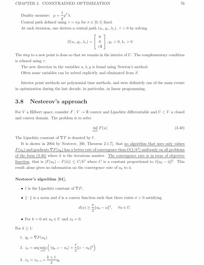
CHAPTER 3. CONSTRAINED OPTIMIZATION 76
Duality measure: μ =1
qyTλ.
Central path defined using τ = σμ for σ ∈ [0, 1] fixed.
At each iteration, one derives a central path (uτ , yτ , λτ ), τ > 0 by solving
S(uτ , yτ , λτ) =
⎡⎣ 00τ1l
⎤⎦ , yτ > 0, λτ > 0
The step to a new point is done so that we remain in the interior of U . The complementary condition
is relaxed using τ .
The new direction in the variables u, λ, y is found using Newton’s method.
Often some variables can be solved explicitly and eliminated from S.
Interior point methods are polynomial time methods, and were definitely one of the main events
in optimization during the last decade, in particular, in linear programming.
3.8 Nesterov’s approach
For V a Hilbert space, consider F : V → R convex and Lipschitz differentiable and U ⊂ V a closed
and convex domain. The problem is to solve
infu∈U
F (u) (3.40)
The Lipschitz constant of ∇F is denoted by �.
It is shown in 2004 by Nesterov, [60, Theorem 2.1.7], that no algorithm that uses only values
F (uk) and gradients∇F (uk) has a better rate of convergence than O(1/k2) uniformly on all problems
of the form (3.40) where k is the iterations number. The convergence rate is in term of objective
function, that is |F (uk) − F (u)| ≤ C/k2 where C is a constant proportional to �‖u0 − u‖2. This
result alone gives no information on the convergence rate of uk to u.
Nestorov’s algorithm [61].
• � is the Lipschitz constant of ∇F ;
• ‖ · ‖ is a norm and d is a convex function such that there exists σ > 0 satisfying
d(u) ≥ σ
2‖u0 − u‖2, ∀u ∈ U.
• For k = 0 set u0 ∈ U and x0 = 0.
For k ≥ 1:
1. ηk = ∇F (uk)
2. zk = argminz∈U
(〈ηk, z − uk〉+ �
2‖z − uk‖2
)3. xk = xk−1 +
k + 1
2ηk
CHAPTER 3. CONSTRAINED OPTIMIZATION 77
4. wk = argminw∈U
(�d(w)
σ+ 〈xk, w〉
)
5. uk+1 =2
k + 3wk +
k + 1
k + 3zk
Proposition 3 ([61]) This algorithm satisfies
0 ≤ F (uk)− F (u) ≤ 4�d(u)
σ(k + 1)(k + 2)
The rationale: similarly to CG, one computes the direction at iteration k by using the information
in{∇F (uk−1), · · · ,∇F (u0)
}.
For details and applications in image processing, see [9] and [88].
Y. Nesterov proposes an accelerated algorithm in [59] where the estimation of the Lipschitz
constant is adaptive and improved.
Other solvers—see next chapter.
Chapter 4
Non differentiable problems
Textbooks: [38, 73, 45, 46, 93, 14]. If not specified, V is a real Hilbert space again.
4.1 Specificities
4.1.1 Examples
Non-differentiable functions frequently arise in practice.
Minimax problems
Minimize F (u) = maxi∈I ϕi(u) where I is a finite set of indexes and ∀i ∈ I, ϕi is convex and smooth.
Regularized objective functionals on Rn
The minimizers of functionals of the form F (u) = Ψ(u) + βΦ(u) (remind (1.5)-(1.6), p. 7, and the
explanations that follow) are very popular to define a restored image or signal. They are often
used in learning theory, in approximation and in many other fields. Nonsmooth F have attracted a
particular attention because of the specific properties of their solutions.
• Non-differentiable regularization term
Φ(u) =∑i
ϕ(‖Diu‖), with ϕ′(0+) > 0
Note that ϕ′(0+) > 0 entails that Φ is nonsmooth.
– For ϕ(t) = t and Di the discrete approximation of the gradient of u at i, along with
‖.‖ = ‖.‖2 = Total Variation (TV) regularization [76];
For ϕ(t) = t and Di ∈ R1×n = median pixel regularization (approximate TV) [13];
– Other non-differentiable (nonconvex) potential functions ϕ:
∗ ϕ(t) = t
α+ t, see [42, 43] :
∗ ϕ(t) = tα, α ∈]0, 1[– If u = the coefficients of the decomposition of the image in a wavelet basis or a frame
and Di = ei, ∀i, then u = shrinkage estimation of the coefficients [35, 58, 12, 6]). See
Examples 9 (p. 79) and 8 (p. 99).
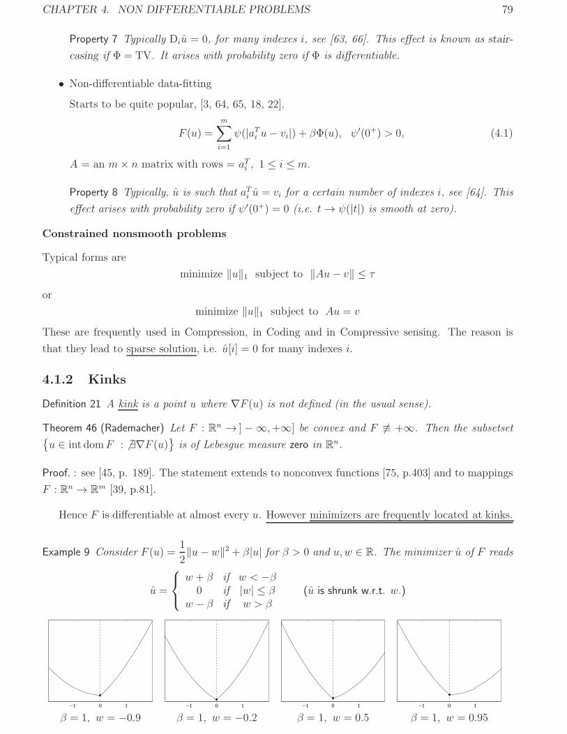
CHAPTER 4. NON DIFFERENTIABLE PROBLEMS 79
Property 7 Typically Diu = 0, for many indexes i, see [63, 66]. This effect is known as stair-
casing if Φ = TV. It arises with probability zero if Φ is differentiable.
• Non-differentiable data-fitting
Starts to be quite popular, [3, 64, 65, 18, 22].
F (u) =
m∑i=1
ψ(|aTi u− vi|) + βΦ(u), ψ′(0+) > 0, (4.1)
A = an m× n matrix with rows = aTi , 1 ≤ i ≤ m.
Property 8 Typically, u is such that aTi u = vi for a certain number of indexes i, see [64]. This
effect arises with probability zero if ψ′(0+) = 0 (i.e. t→ ψ(|t|) is smooth at zero).
Constrained nonsmooth problems
Typical forms are
minimize ‖u‖1 subject to ‖Au− v‖ ≤ τ
or
minimize ‖u‖1 subject to Au = v
These are frequently used in Compression, in Coding and in Compressive sensing. The reason is
that they lead to sparse solution, i.e. u[i] = 0 for many indexes i.
4.1.2 Kinks
Definition 21 A kink is a point u where ∇F (u) is not defined (in the usual sense).
Theorem 46 (Rademacher) Let F : Rn → ] −∞,+∞] be convex and F �≡ +∞. Then the subsetset{u ∈ int domF : � ∃∇F (u)} is of Lebesgue measure zero in R
n.
Proof. : see [45, p. 189]. The statement extends to nonconvex functions [75, p.403] and to mappings
F : Rn → Rm [39, p.81].
Hence F is differentiable at almost every u. However minimizers are frequently located at kinks.
Example 9 Consider F (u) =1
2‖u− w‖2 + β|u| for β > 0 and u, w ∈ R. The minimizer u of F reads
u =
⎧⎨⎩w + β if w < −β
0 if |w| ≤ βw − β if w > β
(u is shrunk w.r.t. w.)
−1 0 1 −1 0 1 −1 0 1 −1 0 1
β = 1, w = −0.9 β = 1, w = −0.2 β = 1, w = 0.5 β = 1, w = 0.95
CHAPTER 4. NON DIFFERENTIABLE PROBLEMS 80
4.2 Basic notionsDefinition 22 Γ0(V ) is the class of all l.s.c. convex proper functions on V (a real Hilbert space) .
(Remind Definitions 2, 4 and 6 on p. 10.)
4.2.1 Preliminaries
Definition 23 f : V → R ∪ {+∞}, is said to be positively homogeneous if f(νu) = νf(u), ∀ν >
0, ∀u ∈ V .
Definition 24 f : V → R ∪ {+∞}, is said to be sublinear if it is convex and positively homogeneous.
Lemma 9 f is positively homogeneous
⇐⇒ f(νu) ≤ νf(u), ∀ν > 0, ∀u ∈ V
Proof. (⇒) is obvious. Next—(⇐). Let f(νu) ≤ νf(u), ∀ν > 0, ∀u ∈ V . Since νu ∈ V and ν−1 > 0
f(u) = f(ν−1νu) ≤ ν−1f(νu) ⇔ νf(u) ≤ f(νu), ∀ν > 0, ∀u ∈ V
hence f(νu) = νf(u), ∀ν > 0, ∀u ∈ V . �
Proposition 4 f is sublinear ⇔ f(νu+ μv) ≤ νf(u) + μf(v), ∀(u, v) ∈ V 2, ∀ν > 0, ∀μ > 0
Proof. (⇒) Set η = ν + μ. Using the convexity of f for 1− μ
η=ν
η> 0,
f(νu+ μv)︸ ︷︷ ︸ = f
(η
(ν
ηu+
μ
ηv
))= ηf
(ν
ηu+
μ
ηv
)≤︸︷︷︸ η
(ν
ηf(u) +
μ
ηf(v)
)= νf(u) + μf(v)︸ ︷︷ ︸
(4.2)
(⇐) Taking μ+ ν = 1 in (4.2) shows that f is convex. Furthermore
f(νu)︸ ︷︷ ︸ = f(ν2u+
ν
2u)≤︸︷︷︸ 2ν2f(u) = νf(u)︸ ︷︷ ︸ .
f is positively homogeneous by Lemma 9. �
Sublinearity is stronger than convexity—it does not require μ + ν = 1—and weaker than
linearity—it requires that μ > 0, ν > 0.
Definition 25 Suppose that U ⊂ V is nonempty.
• Support function σU (u) = sups∈U〈s, u〉 ∈ R ∪ {∞}
• Indicator function ιU(u) ={
0 if u ∈ U+∞ if u �∈ U
• Distance from u ∈ V to U : dU(u) = infv∈U ‖u− v‖.
CHAPTER 4. NON DIFFERENTIABLE PROBLEMS 81
We denote by f � : V � → R the convex conjugate of the function f : V → R (see (1.10), p. 14).
When U �= ∅ is convex and closed, we have
ι�U(u) = supv∈V
( 〈u, v〉 − ιU(v)) = supv∈U〈u, v〉 = σU(u) and σ�
U(v) = ι��U (v) = ιU(v) (4.3)
where the second part results from Theorem 4 (p. 15).
Proposition 5 (p. 19, [38]) σU is l.s.c. and sub-linear. Moreover
σU (u) <∞ ∀u ∈ V ⇔ U ⊂ V is bounded.
Proposition 6 (p. 12, [38]) Let f be a proper convex function on a real n.v.s. V . The statements
below are equivalent:
1. ∃ O ⊂ V over which F is bounded above;
2. int domF �= ∅ and F is locally Lipschitz there.
Note that this is the kind of functions we deal with in practical optimization problems.
4.2.2 Directional derivatives
Lemma 10 Let F : V → R be convex, where V is a n.v.s. The function
t→ F (u+ tv)− F (u)t
, t ∈ R+
is increasing.
Proof. For any t > 0, choose an arbitrary τ ≥ 0. Set
αdef=
τ
t+ τ, then 1− α =
t
t+ τ
We check that
αu+ (1− α)(u+ (t+ τ)v) =τ
t + τu+
t
t+ τu+
t
t + τ(t+ τ)v = u+ tv
Hence
F (αu+ (1− α)(u+ (t+ τ)v)= F (u+ tv).
Using the last result and the convexity of F yield
F (u+ tv)︸ ︷︷ ︸ = F (αu+ (1− α)(u+ (t + τ)v)
≤︸︷︷︸ τ
t+ τF (u) +
t
t+ τF(u+ (t+ τ)v
)= F (u) +
t
t + τ
(F(u+ (t+ τ)v
)− F (u))︸ ︷︷ ︸It follows that
F (u+ tv)− F (u)t
≤ F(u+ (t + τ)v
)− F (u)t + τ
, ∀t > 0, ∀τ ∈ R+ .
Hence the result. �
CHAPTER 4. NON DIFFERENTIABLE PROBLEMS 82
Definition 26 Let F : V → R be convex and proper. The (one-sided) directional derivative of F at
u ∈ V along the direction of v ∈ V reads
δF (u)(v) = limt↘0
F (u+ tv)− F (u)t
, ∀u ∈ V (4.4)
= inft>0
F (u+ tv)− F (u)t
, ∀u ∈ V (4.5)
Whenever F is convex and proper, the limit in (4.4) always exists (see [38, p. 23]). The definition
in (4.4) is equivalent to (4.5) since by Lemma 10 (p. 81), the function t→ F (u+tv)−F (u)t
, t ∈ R+ goes
to its unique infimum when t↘ 0.
Remark 22 For nonconvex functions, defined on more general spaces, directional derivatives can be
defined only using (4.4); they do exist whenever the limit in (4.4) do exist.
δF (u)(v) is the right-hand side derivative. The left-hand side derivative is −δF (u)(−v).
F convex ⇒ − δF (u)(−v) ≤ δF (u)(v).
When F is differentiable at u in the usual sense, δF (u)(v) = 〈∇F (u), v〉, ∀v ∈ V .
Proposition 7 Let F : V → R be convex and proper. For any u ∈ V fixed, v → δF (u)(v) is sublinear.
Proof. By Definition 26—(4.4), it is obvious that v → δF (u)(v) is positively homogeneous, i.e.
δF (u)(λv) = λδF (u)(v), ∀λ > 0. Let us check that it is convex. Choose μ > 0 and ν > 0 such that
μ+ ν = 1, and v ∈ V and w ∈ V .
F(u+ t(μv + νw)
)− F (u) = F(μ(u+ tv) + ν(u+ tw)
)− (μF (u) + νF (u)
), ∀t > 0
≤ μ(F (u+ tv)− F (u))+ ν
(F (u+ tw)− F (u)), ∀t > 0.
Divide by t > 0
F(u+ t(μv + νw)
)− F (u)t
≤ μF (u+ tv)− F (u)
t+ ν
F (u+ tw)− F (u)t
, ∀t > 0.
For t↘ 0 we get δF (u)(μv + νw) ≤ μδF (u)(v) + νδF (u)(w). �
Proposition 8 If F ∈ Γ0(V ) is Lipschitz with constant � > 0 on B(u, ρ), ρ > 0 then
‖z − u‖ ≤ ρ ⇒ |δF (z)(v)− δF (z)(w)| ≤ �‖v − w‖, ∀v, w ∈ V.
Proof. Let ε > 0 be such that if 0 < t < ε then z + tv ∈ B(u, ρ) and z + tw ∈ B(u, ρ). Then
∣∣F (z + tv)− F (z + tw)∣∣ ≤ t�‖v − w‖, ∀t ∈]0, ε[
⇔ ∣∣F (z + tv)− F (z)− (F (z + tw)− F (z))∣∣ ≤ t�‖v − w‖, ∀t ∈]0, ε[
⇔∣∣∣∣F (z + tv)− F (z)
t− F (z + tw)− F (z)
t
∣∣∣∣ ≤ �‖v − w‖, ∀t ∈]0, ε[.
Taking the limit when t↘ 0 yields the result. �
CHAPTER 4. NON DIFFERENTIABLE PROBLEMS 83
Proposition 9 (1st-order approximation) Let F : Rn → R be convex and proper, with Lipschitz constant
� > 0 and u ∈ Rn. Then ∀ε > 0, ∃ρ > 0 such that
‖v‖ < ρ ⇒ |F (u+ v)− F (u)− δF (u)(v)| ≤ ε‖v‖.
Proof. By contradiction: let ∃ε > 0 and (vk)k∈N with
tkdef= ‖vk‖ ≤ 1
k + 1
such that ∣∣F (u+ vk)− F (u)− δF (u)(vk)∣∣ > εtk = ε‖vk‖, ∀k ∈ N.
‖vk‖tk
= 1, ∀k ∈ N ⇒ vktk∈ {w ∈ R
n : ‖w‖ = 1} (compact set), ∀k ∈ N ⇒ ∃vkj such that
limj→∞
vkjtkj
= v, ‖v‖ = 1 (4.6)
For � > 0 a local Lipschitz constant of F we have
εtkj <∣∣F (u+ vkj)− F (u)− δF (u)(vkj)
∣∣≤ ∣∣F (u+ vkj)− F (u+ tkjv)
∣∣+ ∣∣F (u+ tkjv)− F (u)− δF (u)(tkjv)∣∣+ ∣∣δF (u)(tkjv)− δF (u)(vkj)∣∣
≤ 2�‖vkj − tkjv‖+∣∣F (u+ tkjv)− F (u)− tkjδF (u)(v)
∣∣Note that by Lemma 8 (p. 82) we have
∣∣δF (u)(tkjv)− δF (u)(vkj)∣∣ ≤ �‖tkjv − vkj‖, which is used to
get the last inequality.
Using that limj→∞
tkj = 0 along with the definition of δF in (4.4) (p. 82) and (4.6)
ε ≤ 2� limj→∞
∥∥∥∥vkjtkj − v∥∥∥∥+ lim
j→∞
∣∣∣∣F (u+ tkjv)− F (u)tkj
− δF (u)(v)∣∣∣∣ = 0.
This contradicts the assumption that ε > 0. �
4.2.3 Subdifferentials
For a given space V , the class of all subsets of V is denoted by 2V .
Definition 27 Let F : V → R be convex and proper. The subdifferential of F is the set-valued operator
∂F : V → 2V whose value at u ∈ V is
∂F (u) = {g ∈ V : 〈g, v〉 ≤ δF (u)(v), ∀v ∈ V } (4.7)
= {g ∈ V : F (z) ≥ F (u) + 〈g, z − u〉 , ∀z ∈ V } (4.8)
A subgradient of F at u is a selection g ∈ V such that g ∈ ∂F (u).
If F is differentiable at u then ∂F (u) = {∇F (u)}.
Lemma 11 The two formulations for ∂F in (4.7) and in (4.8), Definition 27, are equivalent.
CHAPTER 4. NON DIFFERENTIABLE PROBLEMS 84
Proof. Since by Lemma 10, the function t → F (u+tv)−F (u)t
, t ∈ R+, has its infimum for t ↘ 0, using
the definition for δF in (4.5), we can write
∂F (u) = {g ∈ V : 〈g, v〉 ≤ δF (u)(v), ∀v ∈ V } =
{g ∈ V : 〈g, v〉 ≤ F (u+ tv)− F (u)
t, ∀v ∈ V, ∀t > 0
}(use z = u+ tv ⇔ v = (z − u)/t) =
{g ∈ V :
1
t〈g, z − u〉 ≤ F (z)− F (u)
t, ∀z ∈ V, ∀t > 0
}= {g ∈ V : 〈g, z − u〉 ≤ F (z)− F (u), ∀z ∈ V }
The conclusion follows from the observation that when (u, v) describe V 2 and t describes R+, then
z = u+ tv describes V . �
Observe that by the definition of ∂F in (4.7) (p. 83),
δF (u)(v) = sup{ 〈g, v〉 : g ∈ ∂F (u)} = σ∂F (u)(v)
where σ is the support function (see Definition 25, p. 80). Moreover,
−δF (u)(−v) ≤ 〈g, v〉 ≤ δF (u)(v), ∀(g, v) ∈ (∂F (u)× V )
Property 9 If F ∈ Γ0(V ), then ∂F is a maximal monotone mapping, i.e.
• it is monotone:
∀u1, u2 ∈ V ⇒ 〈g2 − g1, u2 − u1〉 ≥ 0, ∀g1 ∈ ∂F (u1), g2 ∈ ∂F (u2)
• and maximal: g1 ∈ ∂F (u1) ⇒ g2 ∈ ∂F (u2) whenever the above condition holds.
Property 10 (p. 277, [56]) Let F ∈ Γ0(V ). Then the set {∂F (u)} is closed and convex.
Proposition 10 (p. 263, [87]) Let G ∈ Rm×n and F : Rn → R read
F (u) = ‖Gu‖2
Then
∂F (u) =
⎧⎪⎪⎨⎪⎪⎩GTGu
‖Gu‖2 if Gu �= 0
{GTh | ‖h‖2 ≤ 1, h ∈ R
m}
if Gu = 0
(4.9)
Proof. Form the definition of the subdifferential (see Definition 27)
∂F (u) ={g ∈ R
n | ‖Gz‖2 − ‖Gu‖2 ≥ 〈g, z − u〉 , ∀z ∈ Rn}
(4.10)
If Gu �= 0 then F is differentiable at u and ∂F (u) = {∇F (u)}, hence the result 1.
1Let fdef= ‖u‖2 =
(∑i u[i]
2). Then
u �= 0 ⇒ ∇f(u) = u
‖u‖2We have F = f ◦G. For Gu �= 0, noticing that ∇Gu = GT , chain rule entails the first equation in (4.9).
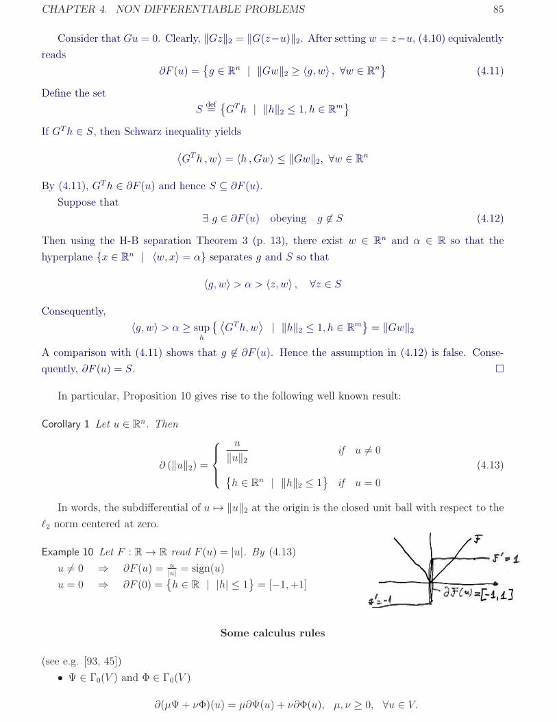
CHAPTER 4. NON DIFFERENTIABLE PROBLEMS 85
Consider that Gu = 0. Clearly, ‖Gz‖2 = ‖G(z−u)‖2. After setting w = z−u, (4.10) equivalentlyreads
∂F (u) ={g ∈ R
n | ‖Gw‖2 ≥ 〈g, w〉 , ∀w ∈ Rn}
(4.11)
Define the set
Sdef=
{GTh | ‖h‖2 ≤ 1, h ∈ R
m}
If GTh ∈ S, then Schwarz inequality yields⟨GTh , w
⟩= 〈h ,Gw〉 ≤ ‖Gw‖2, ∀w ∈ R
n
By (4.11), GTh ∈ ∂F (u) and hence S ⊆ ∂F (u).
Suppose that
∃ g ∈ ∂F (u) obeying g �∈ S (4.12)
Then using the H-B separation Theorem 3 (p. 13), there exist w ∈ Rn and α ∈ R so that the
hyperplane {x ∈ Rn | 〈w, x〉 = α} separates g and S so that
〈g, w〉 > α > 〈z, w〉 , ∀z ∈ S
Consequently,
〈g, w〉 > α ≥ suph
{ ⟨GTh, w
⟩ | ‖h‖2 ≤ 1, h ∈ Rm}= ‖Gw‖2
A comparison with (4.11) shows that g �∈ ∂F (u). Hence the assumption in (4.12) is false. Conse-
quently, ∂F (u) = S. �
In particular, Proposition 10 gives rise to the following well known result:
Corollary 1 Let u ∈ Rn. Then
∂ (‖u‖2) =
⎧⎪⎨⎪⎩u
‖u‖2 if u �= 0
{h ∈ R
n | ‖h‖2 ≤ 1}
if u = 0
(4.13)
In words, the subdifferential of u �→ ‖u‖2 at the origin is the closed unit ball with respect to the
�2 norm centered at zero.
Example 10 Let F : R→ R read F (u) = |u|. By (4.13)
u �= 0 ⇒ ∂F (u) = u|u| = sign(u)
u = 0 ⇒ ∂F (0) ={h ∈ R | |h| ≤ 1
}= [−1,+1]
Some calculus rules
(see e.g. [93, 45])
• Ψ ∈ Γ0(V ) and Φ ∈ Γ0(V )
∂(μΨ+ νΦ)(u) = μ∂Ψ(u) + ν∂Φ(u), μ, ν ≥ 0, ∀u ∈ V.
CHAPTER 4. NON DIFFERENTIABLE PROBLEMS 86
• Ψ ∈ Γ0(V ) and Φ ∈ Γ0(V )
∂(Ψ(u) + Φ(v)
)= ∂Ψ(u)× ∂Φ(v), ∀u ∈ V, ∀v ∈ V.
• A : V →W bounded linear operator, A∗ its adjoint, b ∈ W and F ∈ Γ0(W )
∂(F ◦ (Au+ b)
)(u) = A∗ ◦ ∂F (Au+ b)
• Ψ ∈ Γ0(W ), Φ ∈ Γ0(V ), A : V →W bounded linear operator, 0 ∈ int(dom(Ψ−A(domΦ)
)∂(Ψ ◦ A+ Φ) = A∗ ◦ (∂Ψ) ◦ A+ ∂Φ
• Let U ⊂ V be nonempty, convex and closed. For any u ∈ V \U we have ∂dU (u) =
{u−ΠUu
dU(u)
}.
Duality relations
Theorem 47 Let F ∈ Γ0(V ) and F � : V � → R be its convex conjugate (see (1.10), p. 14). Then
v ∈ ∂F (u) ⇔ F (u) + F �(v) = 〈u, v〉 ⇔ u ∈ ∂F �(v) (4.14)
Proof By (4.8) and using that F = F �� (see Theorem 4, p. 15):
v ∈ ∂F (u)︸ ︷︷ ︸ ⇔ F (z) ≥ F (u) + 〈v, z − u〉 , ∀z ∈ V⇔ 〈v, z〉 − F (z) ≤ 〈v, u〉 − F (u), ∀z ∈ V⇔ F �(v) = sup
z∈V
{〈v, z〉 − F (z)
}= 〈v, u〉 − F (u),
⇔ F �(v) = 〈v, u〉 − F (u)⇔︸︷︷︸ F (u) + F �(v) = 〈u, v〉︸ ︷︷ ︸⇔ F �(v) + F ��(u) = 〈u, v〉 ⇔ u ∈ ∂F �(v)︸ ︷︷ ︸ �
Corollary 2 We posit the conditions of Theorem 47. Then
∂F (u) = {v ∈ V : F (u) + F ∗(v) = 〈u, v〉} .
Continuity properties of the subdifferential of F ∈ Γ0(Rn)
Theorem 48 (Mean-value theorem.) Let F : Rn → R be convex and proper. If u �= v then ∃θ ∈ (0, 1)
and ∃g ∈ ∂F (θv + (1− θ)u) such that
F (v)− F (u) = 〈g, v − u〉
Proof—see [45, p.257].
Property 11 ([45]) ∂F (u) is compact for any u ∈ Rn.
Property 12 ( p.282, [45]) u→ ∂F (u) is locally bounded: B ⊂ Rn bounded ⇒ ∂F (B) ⊂ R
n bounded.
CHAPTER 4. NON DIFFERENTIABLE PROBLEMS 87
Moreover [p. 282, [45]]:
• B ⊂ Rn compact ⇒ ∂F (B) compact.
• B ⊂ Rn compact and connected ⇒ ∂F (B) compact and connected.
• B ⊂ Rn convex — in general ∂F (B) is not convex.
Theorem 49 (Continuity) ∂F is outer semi-continuous at any u ∈ Rn :
∀ε > 0∃ρ > 0 : ‖u− v‖ ≤ ρ ⇒ ∂F (v) ⊂ ∂F (u) +B(0, ε).
Proof—see [45, p.283]
Corollary 3 (p. 283 [45]) For F : Rn → R convex, the function u → δF (u)(v) is upper semi-
continuous:
u ∈ Rn ⇒ δF (u)(v) = lim sup
z→uδF (z)(v), ∀v ∈ R
n.
4.3 Optimality conditions
4.3.1 Unconstrained minimization problems
Theorem 50 (Necessary and Sufficient condition for a minimum) Let F ∈ Γ0(V ), then
F (v) ≥ F (u), ∀v ∈ V ⇔ 0 ∈ ∂F (u) ⇔ δF (u)(v) ≥ 0, ∀v ∈ V.
Proof. Using Definition 27, (4.8) (p. 83)
g = 0 ∈ ∂F (u) ⇔ F (v) ≥ F (u) + 〈0, v − u〉 , ∀v ∈ V ⇔ F (v) ≥ F (u), ∀v ∈ V
Using Definition 27, (4.7), namely ∂F (u) = {g ∈ V : 〈g, v〉 ≤ δF (u)(v), ∀v ∈ V },
g = 0 ∈ ∂F (u) ⇔ 0 ≤ δF (u)(v), ∀v ∈ V
The proof is complete. �
Denote the set of minimizers of F by
U = {u∣∣u ∈ (∂F )−1(0)} (4.15)
The set U is closed and convex.
Remark 23 If F is strictly convex and coercive, then U = {u}, i.e. the minimizer is unique.
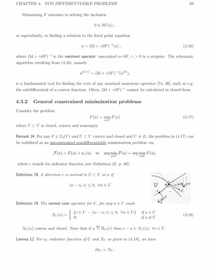
CHAPTER 4. NON DIFFERENTIABLE PROBLEMS 88
Minimizing F amounts to solving the inclusion
0 ∈ ∂F (u) ,
or equivalently, to finding a solution to the fixed point equation
u = (Id + γ∂F )−1(u) , (4.16)
where (Id + γ∂F )−1 is the resolvent operator associated to ∂F , γ > 0 is a stepsize. The schematic
algorithm resulting from (4.16), namely
u(k+1) = (Id + γ∂F )−1(u(k)),
is a fundamental tool for finding the root of any maximal monotone operator [74, 36], such as e.g.
the subdifferential of a convex function. Often, (Id + γ∂F )−1 cannot be calculated in closed-form.
4.3.2 General constrained minimization problems
Consider the problem
F (u) = minu∈U
F (u) (4.17)
where U ⊂ V is closed, convex and nonempty.
Remark 24 For any F ∈ Γ0(V ) and U ⊂ V convex and closed and U �= ∅, the problem in (4.17) can
be redefined as an unconstrained nondifferentiable minimization problem via
F(u) = F (u) + ιU(u) ⇔ argminu∈VF(u) = argmin
u∈UF (u).
where ι stands for indicator function (see Definition 25, p. 80).
Definition 28 A direction v is normal to U ⊂ V at u if
〈w − u, v〉 ≤ 0, ∀w ∈ U
Definition 29 The normal cone operator for U , for any u ∈ U reads
NU (u) =
{ {v ∈ V : 〈w − u, v〉 ≤ 0, ∀w ∈ U} if u ∈ U∅ if u �∈ U (4.18)
NU(u) convex and closed. Note that if udef= ΠU(v) then v − u ∈ NU(u), ∀v ∈ V.
Lemma 12 For ιU indicator function of U and NU as given in (4.18), we have
∂ιU = NU .
CHAPTER 4. NON DIFFERENTIABLE PROBLEMS 89
Proof. By Corollary 2 (p. 86) and using that ι∗U(v) = supz∈U 〈z, v〉 = σU (v). For σU (v) remind
Definition 25 on p. 80 and (4.3) on p. 81.
∂ιU(u) = {v ∈ V : ιU(u) + ι∗U(v) = 〈u, v〉} = {v ∈ V : ιU(u) + supz∈U〈z, v〉 = 〈u, v〉}
If u �∈ U , obviously ∂ιU(u) = ∅. Consider next that u ∈ U in which case ιU(u) = 0. We obtain:
∂ιU(u) = {v ∈ V : supz∈U〈z, v〉 = 〈u, v〉}
= {v ∈ V : 〈z, v〉 ≤ 〈u, v〉 , ∀z ∈ U} �
Theorem 51 Let F ∈ Γ0(V ) and U ⊂ V be closed, convex and nonempty. Then
F (u) = minu∈U
F (u) ⇔ δF (u)(v − u) ≥ 0, ∀v ∈ U ⇔ 0 ∈ ∂F (u) +NU(u)
Proof. ∀v ∈ U and t ∈]0, 1] we have u+ t(v − u) ∈ U .
F (u) = minu∈U
F (u) ⇔ F(u+ t(v − u)) ≥ F (u), ∀t ∈]0, 1], ∀v ∈ U
⇔ F(u+ t(v − u))− F (u)
t≥ 0, ∀t ∈]0, 1], ∀v ∈ U
⇔ inft∈]0,1]
F(u+ t(v − u))− F (u)
t≥ 0, ∀t ∈]0, 1], ∀v ∈ U
⇔ δF (u)(v − u) ≥ 0, ∀v ∈ U. (4.19)
By Lemma 12 (p. 88) we get
∂F (u) +NU(u) = ∂F (u) + ∂ιU(u) = ∂(F (u) + ιU(u)
).
Using Theorem 50 (p. 87) and Remark 24 (p. 88),
F (u) = minu∈U
F (u) ⇔ 0 ∈ ∂(F (u) + ιU(u)) = ∂F (u) +NU(u)
which establishes the last equivalence in the theorem. �
Remark 25 If U = V , the condition of Theorem 51 reads: δF (u)(v) ≥ 0, ∀v ∈ V .
4.3.3 Minimality conditions under explicit constraints
Consider problem (4.17), namely F (u) = minu∈U
F (u), for hi ∈ Γ0(Rn), 1 ≤ i ≤ q
U =
{u ∈ R
n :〈ai, u〉 = bi, 1 ≤ i ≤ p (Au = b ∈ R
p)hi(u) ≤ 0, 1 ≤ i ≤ q
}�= ∅ (4.20)
The set of active constraints at u reads I(u)def= {i : hi(u) = 0}
Theorem 52 ([45], Theorem 2.1.4 (p. 305) and Proposition 2.2.1 (p. 308).) Consider U as in (4.20)
and F ∈ Γ0(Rn) Then the following statements are equivalent:
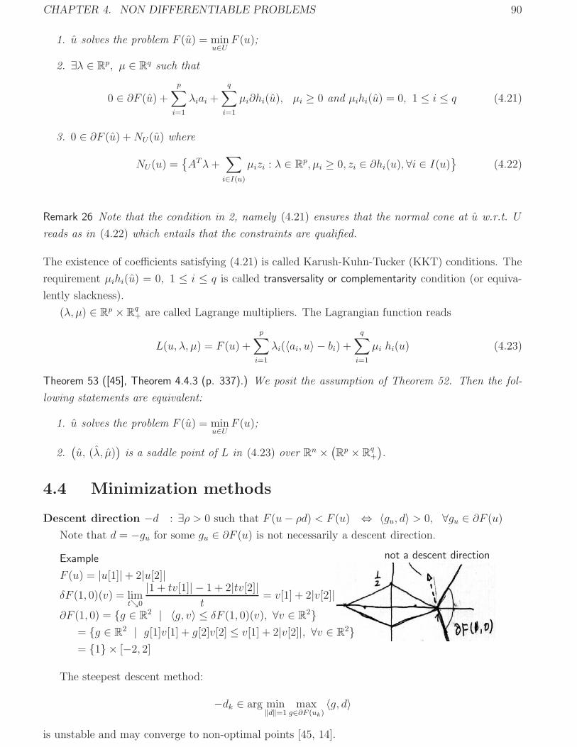
CHAPTER 4. NON DIFFERENTIABLE PROBLEMS 90
1. u solves the problem F (u) = minu∈U
F (u);
2. ∃λ ∈ Rp, μ ∈ R
q such that
0 ∈ ∂F (u) +p∑
i=1
λiai +
q∑i=1
μi∂hi(u), μi ≥ 0 and μihi(u) = 0, 1 ≤ i ≤ q (4.21)
3. 0 ∈ ∂F (u) +NU(u) where
NU(u) ={ATλ+
∑i∈I(u)
μizi : λ ∈ Rp, μi ≥ 0, zi ∈ ∂hi(u), ∀i ∈ I(u)
}(4.22)
Remark 26 Note that the condition in 2, namely (4.21) ensures that the normal cone at u w.r.t. U
reads as in (4.22) which entails that the constraints are qualified.
The existence of coefficients satisfying (4.21) is called Karush-Kuhn-Tucker (KKT) conditions. The
requirement μihi(u) = 0, 1 ≤ i ≤ q is called transversality or complementarity condition (or equiva-
lently slackness).
(λ, μ) ∈ Rp × R
q+ are called Lagrange multipliers. The Lagrangian function reads
L(u, λ, μ) = F (u) +
p∑i=1
λi(〈ai, u〉 − bi) +q∑
i=1
μi hi(u) (4.23)
Theorem 53 ([45], Theorem 4.4.3 (p. 337).) We posit the assumption of Theorem 52. Then the fol-
lowing statements are equivalent:
1. u solves the problem F (u) = minu∈U
F (u);
2.(u, (λ, μ)
)is a saddle point of L in (4.23) over R
n × (R
p × Rq+
).
4.4 Minimization methods
Descent direction −d : ∃ρ > 0 such that F (u− ρd) < F (u) ⇔ 〈gu, d〉 > 0, ∀gu ∈ ∂F (u)Note that d = −gu for some gu ∈ ∂F (u) is not necessarily a descent direction.
not a descent directionExample
F (u) = |u[1]|+ 2|u[2]|δF (1, 0)(v) = lim
t↘0
|1 + tv[1]| − 1 + 2|tv[2]|t
= v[1] + 2|v[2]|∂F (1, 0) = {g ∈ R
2 | 〈g, v〉 ≤ δF (1, 0)(v), ∀v ∈ R2}
= {g ∈ R2 | g[1]v[1] + g[2]v[2] ≤ v[1] + 2|v[2]|, ∀v ∈ R
2}= {1} × [−2, 2]
The steepest descent method:
−dk ∈ arg min‖d‖=1
maxg∈∂F (uk)
〈g, d〉
is unstable and may converge to non-optimal points [45, 14].

CHAPTER 4. NON DIFFERENTIABLE PROBLEMS 91
Some difficulties inherent to the minimization of non-smooth functions
• Usually one cannot compute ∂F (u), but only some elements g ∈ ∂F (u).
• Stopping rule: 0 ∈ ∂F (uk) is difficult to implement.
An approximation like ‖gk‖ ≤ ε can never be satisfied.
• uk → u, gu ∈ ∂F (u) �⇒ ∃{gk ∈ ∂F (uk)} → gu
• Minimizing a smooth approximation of F may generate large numerical errors while the prop-
erties of the minimizer of F and the one of its smoothed version are usually very different.
• Specialized minimization algorithms are needed.
4.4.1 Subgradient methods
Subgradient projections are significantly easier to implement than exact projections and have been
used for solving a wide range of problems.
Subgradient algorithm with projection
Minimize F : Rn → R subject to the constraint set U (closed, convex, nonempty, possibly = Rn)
For k ∈ N
1. if 0 ∈ ∂F (uk), stop (difficult to verify); else
2. obtain gk ∈ ∂F (uk) (easy in general);
3. (possible) line-search to find ρk > 0;
4. uk+1 = ΠU
(uk − ρk gk
‖gk‖)
Remark 27 −dk = − gk‖gk‖ is not necessarily a descent direction. This entails oscillations of the value
(F (uk))k∈N.
Theorem 54 Suppose that F : Rn → R is convex and reaches its minimum at u ∈ Rn. If (ρk)k≥0
satisfies ∑k
ρk = +∞ and∑k
ρ2k < +∞ ⇒ limk→∞
uk = u. (4.24)
Proof: see [79, 14].
By (4.24), ρk converges fast to 0 which means that the convergence of uk is slow (sub-linear).
(E.g., ρk = 1/(k + 1) for k ∈ N.)

CHAPTER 4. NON DIFFERENTIABLE PROBLEMS 92
An adaptive level-set method for constrained nonsmooth minimization
Following Combettes in [28]
(P ) find u such that F ( u) = minu∈U
F (u)def= μ
where F : Rn → R is convex and proper and U ⊂ Rn is closed, convex and �= ∅.
The lower level set of F at height μ ∈ R:
L(μ)def= {u ∈ R
n : F (u) ≤ μ} is convex and closed.
Note that L(μ) = ∅ if μ < μ.
For μ ∈ R, u ∈ Rn and gu ∈ ∂F (u) define the half-space
H(u, gu, μ) = {v ∈ Rn : 〈gu, u− v〉 ≥ F (u)− μ} .
Let z ∈ L(μ), then F (z) ≤ μ. From the definition of ∂F in (4.8), 〈gu, u− z〉 ≥ F (u)− F (z) ≥F (u)− μ. Then z ∈ H(u, gu, μ), hence
L(μ) ⊂ H(u, gu, μ)
The subgradient projection of u onto H(u, gu, μ) reads (see [27])
Πguμ (u) =
⎧⎪⎪⎨⎪⎪⎩u if F (u) ≤ μ or 0 = g ∈ ∂F (u)
u+μ− F (u)‖gu‖2 gu otherwise
Indeed,⟨gu, u−Πg
μ(u)⟩= F (u)− μ.
If μ is known—Polyak’s method (cf. [79]):
u0 ∈ U, ∀k ∈ N ∂uk
def= gk ∈ ∂F (uk), uk+1 = ΠU ◦ Πgk
μ (uk)k→∞−→ u.
In general μ is unknown. Idea: estimate μ adaptively. Adaptive level-set approach:
u0 ∈ U, ∀k ∈ N gk ∈ ∂F (uk), uk+1 = ΠU ◦ Πgkμk(uk) (4.25)
where (μk)k∈N is a sequence of level estimates.
Let μ is un upper bound of μ.
Theorem 55 ([48]) Let μ ≥ μ and u0 ∈ U . Let uk, k ∈ N be generated by (4.25) with μk ↘ μ when
k →∞. Then limk→∞
uk ∈ L(μ) ∩ U .
Theorem 56 ([2]) Suppose μ ≤ μ and u0 ∈ U . Let uk, k ∈ N be generated by (4.25) with μk = μ,
∀k ∈ N. Then ∀ε ∈]0,∞[, ∃n ∈ N such that F (un) ≤ μ+ (μ− μ) + ε.
These theorems show that if a reasonably tight estimate of μ is available then (P ) can be solved
approximately by (4.25).
Comments on the algorithm proposed in [28]:

CHAPTER 4. NON DIFFERENTIABLE PROBLEMS 93
• Adaptive refinement of the estimated levels μk;
• Explicit criterion to detect infeasibility (μk < μ)
Implementable Algorithm
Determine U = U ∩ U such that u ∈ U . Fix ε > 0, 0 < λ < 1
0. u0 ∈ U , η0 > λε and μ0 = F (u0).
1. Set ρk = 0, y = uk and γ ≥ d(y, U) ; if ηk ≤ λε, stop
2. Obtain gk ∈ ∂F (uk) ; if gk = 0, stop.
3. μk = μk − ηk
4.
⎧⎪⎨⎪⎩v = uk + (μk − F (uk)) gk
‖gk‖2uk+1 = ΠU(v)ρk+1 = ρk + ‖v − uk‖2 + ‖uk+1 − v‖2
5. θ =‖y − uk+1‖
2γ − ‖y − uk+1‖ ,{ρk+1 > θ �→ 6ρk+1 ≤ θ �→ 7
6. ηk+1 = ληk, μk+1 = μk, uk+1 = uk �→ 1
7. ηk+1 = ηk, μk+1 = min{F (uk+1), μk} �→ 2
We need to determine an U as tight as possible in order to get a better convergence rate. Note
that μk ≥ μk+1 ≥ μ. Step 5 = test to check if μk < μ (in which case L(μk) = ∅). If so, one decreases
η in 6. Otherwise, one updates μ in 7.
Remark 27 still holds true, i.e. F (uk)k∈N oscillates. The choice of step-size ρk is improved with
respect to (4.24).
4.4.2 Some algorithms specially adapted to the shape of F
Given the form of F one can often design specific (well adapted) optimization algorithms. There
are numerous examples in the literature. We present some outstanding samples.
TV minimization (Chambolle 2004)
Reference:[16]
Minimize F (u) = 12‖u− v‖22 + βTV(u) where
TV(u) = sup{∫
u(x)divξ(x)dx : ξ ∈ C1c (Ω,R2), |ξ(x)| ≤ 1, ∀x ∈ Ω}
(4.26)
Let u ∈ Rn×n and v ∈ R
n×n. Notations:
• ∇—discrete equivalent for ∇• Div—discrete equivalent for div, defined by Div = −∇∗ : (Rn×n)
2 → Rn×n, ∇∗ is the adjoint of ∇
CHAPTER 4. NON DIFFERENTIABLE PROBLEMS 94
∇ and Div are matrix operators as described below.
(∇u)[i, j] =[u[i+ 1, j]− u[i, j]u[i, j + 1]− u[i, j]
], 1 ≤ i, j ≤ n
with boundary conditions u[n+ 1, i] = u[n, i], u[i, n+ 1] = u[i, n]
Div is hence defined by 〈−Divξ, u〉Rn×n =
⟨ξ, ∇u
⟩Rn×n×Rn×n
. One checks easily that
(Div(ξ))[i, j] =(ξ1[i, j]− ξ1[i− 1, j]
)+(ξ2[i, j]− ξ2[i, j − 1]
), 1 ≤ i, j ≤ n,
boundary conditions: ξ1[0, i] = ξ1[n, i] = ξ2[i, 0] = ξ2[i, n] = 0.
Define
K ={Divξ | ξ ∈ (
Rn×n
)2, ‖(ξ[i, j])‖2 ≤ 1, 1 ≤ i, j ≤ n
} ⊂ Rn×n (4.27)
where ξ[i, j] = (ξ1[i, j], ξ2[i, j]). Let us emphasize that K is convex and closed2.
The discrete equivalent of the TV regularization in (4.26) reads
TV(u) = sup{ 〈u, w〉 : w ∈ K}
= supw∈K〈u, w〉 = σK(u)
Its convex conjugate (see (1.10), p. 14)
TV∗(w) = supu
(〈u, w〉 − TV(u)) = ιK(w)
where we use σ∗K = ιK , see (4.3) (p. 81). Since TV ∈ Γ0(R
n×n), using Fenchel-Moreau Theorem 4
(p. 15), TV(u) = TV∗∗(u).
Using that
∂F (u) = u− v + β∂TV(u),
Theorem 50 (p. 87) implies that F has a minimum at u if and only if
0 ∈ ∂F (u) ⇔ 0 ∈ u− v + β∂TV(u) ⇔ v − uβ∈ ∂TV(u)
(Use Theorem 47 p. 86)⇔ u ∈ ∂TV∗(v − uβ
)⇔ 0 ∈ − u
β+
1
β∂TV∗(w) where w
def=v − uβ
⇔ v
β∈ v
β− u
β+
1
β∂TV∗(w) ⇔ v
β∈ w +
1
β∂TV∗(w)
⇔ 0 ∈ w − v
β+
1
β∂TV∗(w)
⇔ w minimizes the function F below
F(w) = minw∈Rn×n
{1
2
∥∥∥∥w − v
β
∥∥∥∥2
+1
βTV∗(w)
}= min
w∈K
{1
2
∥∥∥∥w − v
β
∥∥∥∥2
2
}⇔
w = ΠK
(v
β
)⇔ u = v − βΠK
(v
β
)(4.28)
2The set K is composed out of “oscillatory” components.

CHAPTER 4. NON DIFFERENTIABLE PROBLEMS 95
where ΠK is the orthogonal projection onto K. To calculate u, we need to find Divξ that solves the
nonlinear projection onto ΠK :
min
{∥∥∥∥Div ξ − v
β
∥∥∥∥2
: ξ ∈ (Rn×n)2, ‖ξ[i, j]‖22 − 1 ≤ 0, 1 ≤ i, j ≤ n
}
KT optimality conditions (Theorem 39, p. 66) ⇒ see [16] for details.
Algorithm:
ξk+1[i, j] =ξk[i, j] + ρ
(∇(Div ξk − v/β
))[i, j]
1 + ρ∣∣∣ (∇(Div ξk − v/β
))[i, j]
∣∣∣Theorem 57 (p. 91, [16]) For ρ ≤ 1/8, convergence of Div ξk to w = ΠK(v/β) as k →∞.
This algorithm amounts to a special instance of Bermudez and Moreno’s Algorithm (1979), see
Aujol 2009 [9]. Hence convergence for ρ ≤ 1/4.
One coordinate at a time when the non-differentiable term is separable
Consider
F (u) = Ψ(u) +
n∑i=1
βiϕi(|u[i]|), βi ≥ 0, ϕi′(0+) > 0, ∀1 ≤ i ≤ n (4.29)
Remark 28 Note that (4.1), namely F (u) =
n∑i=1
ψ(| 〈ai, u〉 − vi|) + βΦ(u), ψ′(0) > 0 can be rewritten
in the form of (4.29), provided that {ai, 1 ≤ i ≤ n} is linearly independent. Let A ∈ Rn×n be the
matrix whose columns are ai, 1 ≤ i ≤ n. Using the change of variables z = Au− v, we consider
F(z) = 1
β
n∑i=1
ψ(|zi|) + Φ(A−1(z − v))
Theorem 58 Let F : Rn → R in (4.29) be convex, proper and coercive, Ψ ∼ C1 be convex, βi ≥ 0
and ϕi : R+ → R be convex, C1 and ϕ′i(0) > 0, 1 ≤ i ≤ n. Suppose that Ψ satisfies only one of the
conditions below:
1. Ψ is coercive;
2. ∀ρ > 0, ∃η > 0 such that ‖u‖ ≤ ρ, |t| ≤ ρ ⇒ Ψ(u+ tei)−Ψ(u) ≥ t∂Ψ(u)
∂ui+ t2η, 1 ≤ i ≤ n.
Then the one coordinate at a time method given in §2.2 (p. 22) converges to a minimizer u of F .
Proof. : under condition 1, see [44]; under condition 2, see [65].
Comments
• Condition 2 is quite loose since it does not require that Ψ is globally coercive.
• The method cannot be extended to Φ non separable.
CHAPTER 4. NON DIFFERENTIABLE PROBLEMS 96
Algorithm.
∀k ∈ N, each iteration k has n steps:
1 ≤ i ≤ n, compute
ξ =∂
∂u[i]Ψ(u(k)[1], . . . , u(k)[i− 1], 0, u(k−1)[i+ 1], . . . , u(k−1)[n]
);
if |ξ| ≤ βiϕ′i(0
+) ⇒ u(k)[i] = 0; (�)
else u[i](k) solves the equation on R \ {0}βiϕ
′i(u
(k)[i]) +∂
∂u[i]Ψ(u(k)[1], . . . , u(k)[i− 1], u(k)[i], u(k−1)[i+ 1], . . . , u(k−1)[n]
)= 0,
where sign(u(k)[i]
)= −sign(ξ)
The components located at kinks are found exactly in (�). Note that for t �= 0, we have ddtϕi(|t|) =
ϕ′i(|t|)sign(t). In particular, for ϕi(t) = |t|, we have good simplifications: ϕ′
i(0+) = 1 and ϕ′
i(t) =
sign(t) if t �= 0.
Useful reformulation
For any w ∈ Rn we consider the decomposition
w = w+ − w− where w+[i] ≥ 0, w−[i] ≥ 0, 1 ≤ i ≤ n
Then
Minimize ‖w‖1 ⇔ minimize∑i
(w+[i] + w−[i]
)subject to w+[i] ≥ 0, w−[i] ≥ 0, 1 ≤ i ≤ n.
Can be used to minimize TV(u) ≈ ‖Du‖1, see [4, 40].
4.4.3 Variable-splitting combined with penalty techniques
We will describe the approach in the context of an objective function F : Rn → R of the form
F (u) = ‖Au− v‖22 + β∑i
‖Diu‖2 = ‖Au− v‖22 + βTV(u) (4.30)
where for any i, Diu ∈ R2 is the discrete approximation of the gradient of u at i. The second
summand is hence the nonsmooth TV regularization [76].
The idea of variable-splitting and penalty techniques in optimization is as follows: with each
nonsmooth term ‖Diu‖2 an auxiliary variable bi ∈ R2 is associated in order to transfer Diu out of
the nondifferentiable term ‖ · ‖2, and the difference between bi and Diu is penalized. The resultant
approximation to (4.30) is
F(u, b) = ‖Au− v‖22 + λ∑i
‖bi − Diu‖22 + β∑i
‖bi‖2 (4.31)
with a sufficiently large penalty parameter λ. This quadratic penalty approach can be traced back
as early as Courant [32] in 1943. It is well known that the solution of (4.31) converges to that of
CHAPTER 4. NON DIFFERENTIABLE PROBLEMS 97
(4.30) as λ→∞. The motivation for this formulation is that, while either one of the two variables
u and b is fixed, minimizing the function with respect to the other has a closed-form formula with
low computational complexity. Indeed, F is quadratic in u and separable in b. A connection with
the additive form of half-quadratic regularization, see (2.36) on p. 39, was investigated in [87]. For
λ fixed, an alternating minimization scheme is applied to F :
uk+1 = arg minu∈Rn
{‖Auk − v‖22 + λ
∑i
‖bik − Diuk‖22}
(4.32)
bik+1= argmin
{λ‖bi − Diuk+1‖22 + β‖bi‖2
}, ∀i (4.33)
Finding uk+1 in (4.32) amounts to solve a linear problem. According to the content of A, fast solvers
have been exhibited (see e.g. [62]).
The computation of bik+1in (4.33) can be done in an exact and fast way using multidimensional
shrinkage suggested in [87] and proven in [91], presented next.
Lemma 13 ([91], p. 577) For α > 0, β > 0 and v ∈ Rn, where n is any positive integer, set
f(u) =α
2‖u− v‖22 + β‖u‖2
The unique minimizer of f is given by
u = max
{‖v‖2 − β
α, 0
}v
‖v‖2 (4.34)
where the convention 0 · (0/0) = 0 is followed.
Proof. Since f is strictly convex, bounded below, and coercive, it has unique minimizer u. Using
Corollary 1 (p. 85), the subdifferential of f reads
∂f(u) = α(u− v) + β
⎧⎪⎨⎪⎩u
‖u‖2 if u �= 0
{h ∈ R
n | ‖h‖2 ≤ 1}
if u = 0
According to the optimality conditions, 0 ∈ ∂f(u), hence⎧⎪⎪⎨⎪⎪⎩α(u− v) + β
u
‖u‖2 = 0 if u �= 0
αv ∈ {h ∈ R
n | ‖h‖2 ≤ β}
if u = 0
From the second condition, it is obvious that
u = 0 ⇔ ‖v‖2 ≤ β
α(4.35)
Consider next that u �= 0. Thenu
‖u‖2
(‖u‖2 + β
α
)= v
It follows that there exists a positive constant c such that u = cv. The latter obeys
v
(c +
β
α‖v‖2 − 1
)= 0 ⇒ c = 1− β
α‖v‖2
CHAPTER 4. NON DIFFERENTIABLE PROBLEMS 98
Note that c > 0 if and only if ‖v‖2 > βα. Hence
u =
(1− β
α‖v‖2
)v =
(‖v‖2 − β
α
)v
‖v‖2 ⇔ ‖v‖2 − β
α> 0 (4.36)
Combining (4.35) and (4.36) leads to (4.34). �
Using Lemma 13, each bik+1in (4.33) read
bik+1= max
{‖Diuk+1‖2 − β
2λ, 0
}Diuk+1
‖Diuk+1‖2A convergence analysis of the relevant numerical scheme is provided in [87]. In the same reference,
it is exhibited how to apply the continuation on λ (i.e. the increasing of λ) in order to improve the
convergence.
Remark 29 If n = 1 in Lemma 13, that is
f(u) =α
2(u− v)2 + β|u|, u ∈ R
then (4.34) amounts to the soft-shrinkage operator
u = max
{|v| − β
α, 0
}sign(v) =
{0 if |v| ≤ β
α
v − βαsign(v) if |v| > β
α
Remind also Example 9 on p. 79.
Similar ideas have recently been used to minimize F (u) = ‖Au − v‖1 + β∑
i ‖Diu‖2 where Di
are quite general matrices in [92] for multichannel image restoration.
4.5 Splitting methods
Let V be a Hilbert space3 and Ψ ∈ Γ0(V ) and Φ ∈ Γ0(V ) Consider the problem
find u = argminuF (u), F (u) = Ψ(u) + Φ(u).
The astuteness of splitting methods for F = Ψ+ Φ is to use separately
proxγΨ = (Id + γ∂Ψ)−1 and proxγΦ = (Id + γ∂Φ)−1
Usually these are much easier to obtain than the resolvent for F , namely proxγF = (Id + γ∂F )−1.
Even though the literature is abundant, these can basically be systematized into three main
classes:
• forward-backward, see [41, 82, 83];
• Douglas/Peaceman-Rachford, see [51];
• double-backward (little-used), see [50, 71].
A recent theoretical overview of all these methods can be found in [29, 37]. They are essentially
based on proximal calculus.
3Hence V = V �.
CHAPTER 4. NON DIFFERENTIABLE PROBLEMS 99
4.5.1 Moreau’s decomposition and proximal calculus
Proximity operators were inaugurated in [57] as a generalization of convex projection operators.
Proposition 11 (p. 278, [56].) Let f ∈ Γ0(V ). For any v ∈ V , the function Pf : V → R below
Pf (u) =1
2‖v − u‖2 + f(u) (4.37)
admits a unique minimizer.
Definition 30 The unique minimizer in Proposition 11 is denoted by
proxf v = argminu∈VPf (u). (4.38)
proxf is the proximity operator for f .
Remark 30 From (4.37) and (4.38), the optimality conditions (Theorem 50, p. 87) yield
u = proxf v ⇔ 0 ∈ ∂Pf (u) ⇔ 0 ∈ u−v+∂f(u) ⇔ v − u ∈ ∂f(u) ⇔ u = (Id+∂f)−1(v) (4.39)
⇔ (Id + ∂f)−1 = proxf
Example 11 Several examples of proxf for f ∈ Γ0(V ):
1. f(u) = 〈a, u〉 − β, a ∈ V , β ∈ R. Then proxf v = v − a (a translation)
2. U ⊂ V is closed, convex and �= ∅. f(u) = ιU(u) then proxιU v = ΠU(v)
3. f(u) = β‖u‖22, β ≥ 0. Then proxf v =1
1 + 2βv
4. f(u) = β‖u‖2, β ≥ 0. Then proxf v = max{‖v‖2 − β, 0} v
‖v‖2 (see Lemma 13, p. 97)
5. f(u) = Ψ(−u) then proxfv = −proxΨ(−v)
6. f(u) = Ψ(u− z), z ∈ V . Then proxf v = z + proxΨ (v − z)
7. f(u) = Ψ(u/β), β ∈ R \ {0}. Then proxf v = βproxΨ/β2 (v/β).
8. f(u) =n∑
i=1
βi∣∣u[i]− z[i]∣∣, βi ≥ 0, ∀i. Then
(proxf v
)[i] = z[i] + T βi
(v[i]− z[i]), ∀i, where
∀β > 0, T β(t)def=
{0 if |t| < βt− βsign(t) otherwise
T β is a soft shrinkage operator
See Remark 29 on p. 98 and Example 9 on p. 79.
9. proxβTVv = v − βΠK(vβ) where K is given in (4.27), p. 94; see (4.28).
Some important properties
Relationship with the classical Projection Theorem:
CHAPTER 4. NON DIFFERENTIABLE PROBLEMS 100
Theorem 59 ([56], p. 280.) Let f ∈ Γ0(V ) and f � ∈ Γ0(V ) be its convex conjugate. For any u, v, w ∈V we have the equivalence
w = u+ v and f(u) + f �(v) = 〈u, v〉 ⇔ u = proxf w, v = proxf� w.
Meaning: Link with the Projection theorem.
Proof. Two parts.
(⇒) By the definition of the convex conjugate4 f �(v) = supz∈V( 〈z, v〉 − f(z)), we have
〈u, v〉 − f(u) = f �(v) ≥ 〈z, v〉 − f(z), ∀z ∈ V ⇒ f(z)− f(u) ≥ 〈z − u, v〉 , ∀z ∈ V (4.40)
Pf(z)− Pf (u)︸ ︷︷ ︸ =1
2‖z − w‖2 + f(z)− 1
2‖u− w‖2 − f(u), ∀z ∈ V
=1
2‖z − u− v‖2 − 1
2‖v‖2 + f(z)− f(u), ∀z ∈ V set v = w − u
≥︸︷︷︸ 1
2‖z − u− v‖2 − 1
2‖v‖2 + 〈z − u, v〉 , ∀z ∈ V (by (4.40))
=1
2‖z − u‖2 − 〈z − u, v〉+ 1
2‖v‖2 − 1
2‖v‖2 + 〈z − u, v〉 , ∀z ∈ V
=1
2‖z − u‖2 ≥ 0︸ ︷︷ ︸, ∀z ∈ V.
It follows that u is the unique point such that Pf (u) < Pf (z), ∀z ∈ V, z �= u. Hence u = proxf w.
In a similar way one establishes that v = proxf� w.
(⇐) Since u = proxf w for w ∈ V , we know that u is the unique minimizer of Pf on V for this w
(see Proposition 11 on p. 99). Hence
Pf
(t(z − u) + u
)=
1
2‖t(z − u) + u− w‖2 + f
(t(z − u) + u
)≥ 1
2‖u− w‖2 + f(u) = Pf (u) =
1
2‖v‖2 + f(u), ∀z ∈ V, t ∈ R
where we set
v = w − uRearranging the obtained inequality yields
1
2‖v‖2 − 1
2‖t(z − u)− v‖2 + f(u) ≤ f
(t(z − u) + u
), ∀z ∈ V, t ∈ R.
Noticing that 12‖v‖2− 1
2‖t(z−u)− v‖2 = −1
2t2‖z−u‖2+ t 〈z − u, v〉, the last inequality entails that
−12t2‖z − u‖2 + t 〈z − u, v〉+ f(u) ≤ f
(t(z − u) + u
), ∀z ∈ V, t ∈ R. (4.41)
Remind that t(z − u) + u = tz + (1− t)u. Since f is convex, for t ∈]0, 1[ we have
f(t(z − u) + u
) ≤ tf(z) + (1− t)f(u) = f(u) + t(f(z)− f(u)), ∀t ∈]0, 1[, ∀z ∈ V.
4This definition was already given in (1.10) on p. 14.
CHAPTER 4. NON DIFFERENTIABLE PROBLEMS 101
Inserting the last inequality into (4.41) leads to
−12t2‖z − u‖2 + t 〈z − u, v〉+ f(u) ≤ t
(f(z)− f(u))+ f(u), ∀t ∈]0, 1[, ∀z ∈ V,
⇔ −12t2‖z − u‖2 + t 〈z − u, v〉 ≤ t
(f(z)− f(u)), ∀t ∈]0, 1[, ∀z ∈ V,
⇔ −12t‖z − u‖2 + 〈z − u, v〉 ≤ f(z)− f(u), ∀t ∈]0, 1[, ∀z ∈ V,
⇔ 〈z, v〉 − f(z) ≤ 〈u, v〉 − f(u) + 1
2t‖z − u‖2, ∀t ∈]0, 1[, ∀z ∈ V.
Letting t→ 0 yields
〈z, v〉 − f(z) ≤ 〈u, v〉 − f(u), ∀z ∈ V.Then
supz∈V
( 〈z, v〉 − f(z)) = f �(v) = 〈u, v〉 − f(u)
Taking v = v = w − u achieves the proof. �
In words, it was proven that ∀w ∈ V , for a given f ∈ Γ0(V ), we have a unique decomposition
w = proxfw + proxf�w
Definition 31 An operator T : V → V is
1. nonexpansive if ‖Tu− Tv‖ ≤ ‖u− v‖, ∀u ∈ V, ∀v ∈ V
2. firmly nonexpansive if ‖Tu− Tv‖2 ≤ 〈Tu− Tv, u− v〉 , ∀u ∈ V, ∀v ∈ V
Hence a firmly nonexpansive operator is always nonexpansive.
Lemma 14 If T : V → V is firmly nonexpansive, then the operator (Id − T ) : V → V is firmly
nonexpansive.
Proof. Using that T is firmly nonexpansive, we obtain that ∀u ∈ V, ∀v ∈ V
‖(Id− T )u− (Id− T )v‖2 − 〈(Id− T )u− (Id− T )v, u− v〉= ‖u− v − (Tu− Tv)‖2 − 〈u− v − (Tu− Tv), u− v〉= ‖Tu− Tv‖2 + ‖u− v‖2 − 2 〈Tu− Tv, u− v〉+ 〈Tu− Tv, u− v〉 − ‖u− v‖2= ‖Tu− Tv‖2 − 〈Tu− Tv, u− v〉 ≤ 0,
where the last inequality comes from Definition 31-2. Hence the result. �
Proposition 12 ([31], Lemma 2.4.) For f ∈ Γ0(V ), proxf and (Id− proxf ) are firmly nonexapnsive
Proposition 13 Let f ∈ Γ0(V ). The operator proxf is monotonous in the sense that⟨proxfw − proxfz , proxf�w − proxf�z
⟩ ≥ 0, ∀w ∈ V, ∀z ∈ V.
CHAPTER 4. NON DIFFERENTIABLE PROBLEMS 102
Proof. For w ∈ V and z ∈ V set
u = proxfw u′ = proxfz
v = proxf�w v′ = proxf�z
Noticing that by Theorem 59 we have
f(u) + f �(v) = 〈u, v〉 and f(u′) + f �(v′) = 〈u′, v′〉 (4.42)
and that by Fenchel-Young inequality (1.11) (p. 14)
f �(v′) ≥ 〈u, v′〉 − f(u) and f(u′) ≥ 〈v, u′〉 − f �(v) (4.43)
we obtain ⟨proxfw − proxfz , proxf�w − proxf�z
⟩= 〈u− u′, v − v′〉
= 〈u, v〉+ 〈u′, v′〉 − 〈u, v′〉 − 〈u′, v〉use (4.42) = f(u) + f �(v) + f(u′)︸ ︷︷ ︸+ f �(v′)︸ ︷︷ ︸−〈u, v′〉 − 〈u′, v〉use (4.43) ≥︸︷︷︸ f(u) + f �(v) + 〈u, v′〉 − f(u) + 〈v, u′〉 − f �(v)− 〈u, v′〉 − 〈u′, v〉 = 0.
The proof is complete. �
4.5.2 Forward-Backward (FB) splitting
Forward-backward can be seen as a generalization of the classical gradient projection method for
constrained convex optimization. One must assume that either Ψ or Φ is differentiable.
Proposition 14 ([31], Proposition 3.1.) Assume that Ψ ∈ Γ0(V ), Φ ∈ Γ0(V ), where V is a Hilbert
space, that Ψ is differentiable and that F = Ψ+ Φ is coercive. Let γ ∈]0,+∞[. Then
F (u) = minu∈V
F (u) ⇔ u = proxγΦ(u− γ∇Ψ(u)
).
Moreover, u is unique if either Ψ of Φ is strictly convex.
Proof. A sequence of equivalences:
F (u) = minu∈V
F (u) ⇔ 0 ∈ ∂(Ψ + Φ)(u) = ∂Ψ(u) + ∂Φ(u) = ∂Φ(u) + {∇Ψ(u)}⇔ −∇Ψ(u) ∈ ∂Φ(u) ⇔ − γ∇Ψ(u) ∈ γ∂Φ(u)⇔ (
u− γ∇Ψ(u))− u ∈ γ∂Φ(u) (use (4.39), p. 99 identify
(u− γ∇Ψ(u)
)with v)
⇔ u = proxγΦ(u− γ∇Ψ(u)
)F is strictly convex if either Ψ of Φ is so, in which case u is unique. �
FB splitting relies on the fixed-point equation
u = proxγΦ(u− γ∇Ψ(u)
)

CHAPTER 4. NON DIFFERENTIABLE PROBLEMS 103
The basic iteration consists in two steps:
uk+ 12
= uk − γ∇Ψ(uk) (forward, explicit)
uk+1 = proxγΦ
(uk+ 1
2
)(backward, implicit)
Formally, the second step amounts to solving an inclusion, hence its implicit nature.
A practical algorithm proposed by Combettes and Wajs in [31] is a more general iteration where
γ is iteration-dependent, errors are allowed in the evaluation of the operators proxγΦ and ∇Ψ and a
relaxation sequence (λk)k∈N is introduced. Admission of errors allows some tolerance in the numerical
implementation of the algorithm, while the iteration-dependent parameters (γk)k∈N and (λk)k∈N can
improve its convergence speed.
Theorem 60 ([31], Theorem 3.4.) Assume that Ψ ∈ Γ0(V ), Φ ∈ Γ0(V ), where V is a Hilbert space,
that Ψ is differentiable with a 1/β-Lipschitz gradient, β ∈]0,∞[, and that F = Ψ + Φ is coercive.
Let the sequences (γk)k∈N ⊂ R+, (λk)k∈N ⊂ R+, (ak)k∈N ⊂ V and (bk)k∈N ⊂ V satisfy
• 0 < infk∈N
γk ≤ supk∈N
γk < 2β;
• 0 < infk∈N
λk ≤ supk∈N
λk ≤ 1;
•∑k∈N‖ak‖ < +∞ and
∑k∈N‖bk‖ < +∞.
Consider the iteration:
uk+1 = uk + λk
(proxγkΦ
(uk − γk(∇Ψ(uk) + bk
)+ ak − uk
), k ∈ N.
Then
1. (uk)k∈N converges weakly to u ∈ U .
2. (uk)k∈N converges strongly to u ∈ U if one of the following conditions hold:
• intU �= ∅;
• either Ψ or Φ satisfy the condition below on U :
f ∈ Γ0(V ); ∀(vk)k∈N, ∀(wk)k∈N belonging to V and v ∈ V and v ∈ ∂f(w) ∈ V we have[wk ⇀ w, vk ⇀ v, vk ∈ ∂f(wk), ∀k ∈ N
] ⇒ w is a strong cluster point of (wk)k∈N.
Let us emphasize that if V = Rn, convergence is always strong.
4.5.3 Douglas-Rachford splitting
Douglas-Rachford splitting, generalized and formalized in [51], is a much more general class of
monotone operator splitting methods. A crucial property of the Douglas-Rachford splitting scheme
is its high robustness to numerical errors that may occur when computing the proximity operators
proxΨ and proxΦ, see [29].
CHAPTER 4. NON DIFFERENTIABLE PROBLEMS 104
Proposition 15 ([30], Proposition 18.) Assume that Ψ ∈ Γ0(V ), Φ ∈ Γ0(V ) and that F = Ψ + Φ is
coercive. Let γ ∈]0,+∞[. Then
F (u) = minu∈V
F (u) ⇔ u = proxγΦz where z =((2proxγΨ − Id) ◦ (2proxγΦ − Id)
)(z).
Moreover, u is unique if either Ψ or Φ is strictly convex.
Given a function f , the expression (2proxf − Id) is also called reflection operator.
Proof. Since F is coercive, U �= ∅. The following chain of equivalences yields the result.
F (u) = infu∈V
F (u) ⇔ 0 ∈ ∂F (u) ⇔ 0 ∈ (∂Ψ + ∂Φ)(u) ⇔ 0 ∈ γ∂Ψ(u) + γ∂Φ(u)
⇔ ∃z ∈ V :
⎧⎨⎩u− z ∈ γ∂Ψ(u) ⇔ 2u− z ∈ (Id + γ∂Ψ)(u)
z − u ∈ γ∂Φ(u) ⇔ z ∈ (Id + γ∂Φ)(u) ⇔ u = (Id + γ∂Φ)−1(z) (a)
⇔ ∃z ∈ V :
⎧⎨⎩2(Id + γ∂Φ)−1(z)− z ∈ (Id + γ∂Ψ)(u) (use (a) for u)
u = (Id + γ∂Φ)−1(z)
⇔ ∃z ∈ V :
⎧⎨⎩(2(Id + γ∂Φ)−1 − Id
)z ∈ (Id + γ∂Ψ)(u)
u = (Id + γ∂Φ)−1(z)
⇔ ∃z ∈ V :
⎧⎨⎩u =(Id + γ∂Ψ)−1 ◦ (2(Id + γ∂Φ)−1 − Id
)(z) = proxγΨ ◦
(2proxγΦ − Id
)(z) (b)
u = proxγΦz (c)
⇔ ∃z ∈ V :
⎧⎨⎩z = 2u− (2u− z) = 2proxγΨ ◦
(2proxγΦ − Id
)(z)− (2proxγΦ − Id)(z)
u = proxγΦz (above: insert (b) for the first 2u and (c) for the second term)
⇔ ∃z ∈ V :
⎧⎨⎩z = (2proxγΨ − Id) ◦ (2proxγΦ − Id
)z
u = proxγΦz
F is coercive by assumption. When either Ψ of Φ is strictly convex, F is strictly convex as well.
Hence F admits a unique minimizer u. �
Thus DR splitting is based on the fixed point equation
z = (2proxγΨ − Id) ◦ (2proxγΦ − Id)(z)
and F reaches its minimum at u = proxγΦz where z is the fixed point of the equation above.
Remark 31 Note that the roles of Φ and Ψ can be interchanged since they share the same assumptions.
CHAPTER 4. NON DIFFERENTIABLE PROBLEMS 105
Given a fixed scalar γ > 0 and a sequence λk ∈ (0, 2), this class of methods can be expressed via
the following recursion written in a compact form
z(k+1) =
((1− λk
2
)Id +
λk2(2proxγΨ − Id) ◦ (2proxγΦ − Id)
)z(k)
A robust DR algorithm is proposed by Combettes and Pesquet in [30].
Theorem 61 ([30], Theorem 20.) Assume that Ψ ∈ Γ0(V ), Φ ∈ Γ0(V ) and that F = Ψ+Φ is coercive
and γ ∈]0,∞[. Let the sequences (λk)k∈N ⊂ R+, (ak)k∈N ⊂ V and (bk)k∈N ⊂ V satisfy
(i) 0 < λk < 2, ∀k ∈ N and∑k∈N
λk(2− λk) = +∞;
(ii)∑k∈N
λk(‖ak‖+ ‖bk‖) < +∞.
Consider the iteration for k ∈ N:
zk+ 12
= (2proxγΦ − Id)zk + bk
zk+1 = zk + λk
(proxγΨ(2zk+ 1
2− zk) + ak − zk+ 1
2
)Then (zk)k∈N converges weakly to a point z ∈ V and
u = proxγΦz = argminu∈V
F (u).
When V is of finite dimension, e.g. V = Rn, the sequence (zk)k∈N converges strongly.
The sequences ak and bk model the numerical errors when computing the proximity operators.
They are under control using (ii). Conversely, if the convergence rate can be established, one can
easily derive a rule on the number of inner iterations at each outer iteration k such that (ii) is
verified.
This algorithm naturally inherits the splitting property of the Douglas-Rachford iteration, in the
sense that the operators proxγΨ and proxγΦ are used in separate steps. Note that the algorithm
allows for the inexact implementation of these two proximal steps via the incorporation of the error
terms ak and bk. Moreover, a variable relaxation parameter λk enables an additional flexibility.
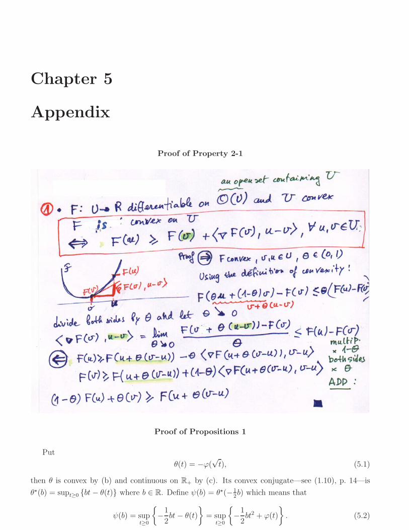
Chapter 5
Appendix
Proof of Property 2-1
Proof of Propositions 1
Put
θ(t) = −ϕ(√t), (5.1)
then θ is convex by (b) and continuous on R+ by (c). Its convex conjugate—see (1.10), p. 14—is
θ�(b) = supt≥0 {bt− θ(t)} where b ∈ R. Define ψ(b) = θ�(−12b) which means that
ψ(b) = supt≥0
{−12bt− θ(t)
}= sup
t≥0
{−12bt2 + ϕ(t)
}. (5.2)
CHAPTER 5. APPENDIX 107
By Theorem 4, p. 15, we have (θ�)� = θ. Calculating (θ�)� at t2 and using (5.1) yields
−ϕ(t) = θ(t2) = supb≤0
{bt2 − θ�(b)} = sup
b≥0
{−12bt2 − ψ(b)
}.
Since θ(t) ≤ 0 on R+, we have θ�(b) = +∞ if b > 0 and then the supremum of b → bt2 − θ�(b) in
the middle expression above necessarily corresponds to b ≤ 0. Finally,
ϕ(t) = infb≥0
{1
2bt2 + ψ(b)
}. (5.3)
The statement ϕ⇒ ψ comes from the fact that (θ�)� = θ.
Next we focus on the possibility to achieve the supremum in ψ jointly with the infimum in ϕ.
For any b > 0, define fb : R+ → R by fb(t) = 12bt + θ(t), then (5.2) yields ψ(b) = − inft≥0 fb(t).
Observe that fb is convex by (b) with fb(0) = 0 by (a) and limt→∞ fb(t) = +∞ by (e), hence fb has
a unique minimum reached at a t ≥ 0. According to (5.2), ψ(b) = −12bt2 + ϕ(t), then equivalently
the infimum in (5.3) is reached for b since ϕ(t) = 12bt2 + ψ(b). Notice that θ′(t) = −ϕ′(
√t)
2√t
and that
f ′b(t) = 1
2b+θ′(t) is increasing on R+ by (b). If f ′
b(0+) ≥ 0, i.e. if b ≥ ϕ′′(0+), fb reaches its minimum
at t = 0. Otherwise, its minimum is reached for a t > 0 such that f ′b(t) = 0, i.e. b = −2θ′(t). In
this case, t→ −12bt2 + ϕ(t) in the last expression of (5.2) reaches its supremum for a t that satisfies
b = −2θ′(t2). Hence b is as given in the proposition.
Derivation of the CG algorithm
Assume that ∇F (uk) �= 0, then the optimal g(αk) �= 0 for αk ∈ Rk+1 is the unique point defined by
(2.40). Then for all iterates 0 ≤ j ≤ k, we have g(αj) �= 0. We will express g(αj) in the form
g(αj) = ρjdj =
j∑i=0
αj [i]∇F (ui), 0 ≤ j ≤ k, dj ∈ Rn, ρj ∈ R (5.4)
Since g(αj) �= 0, we have dj �= 0 and ρj �= 0, 0 ≤ j ≤ k. We will choose dj in such a way that
successive directions are easy to compute. Iterates read
uj+1 = uj − ρjdj = uj −j∑
i=0
αj[i]∇F (ui), 0 ≤ j ≤ k (5.5)
(a) A major result. Combining (2.38) and (5.5),
∇F (uj+1) = ∇F (uj − ρjdj) = ∇F (uj)− ρjBdj , 0 ≤ j ≤ k. (5.6)
For k ≥ 1, combining (2.41) and (5.6) yields
0 = 〈∇F (uj+1),∇F (ui)〉 = 〈∇F (uj),∇F (ui)〉−ρj 〈Bdj,∇F (ui)〉 = −ρj〈Bdj,∇F (ui)〉, 0 ≤ i < j ≤ k.
By (5.12), dj is a linear combination of ∇F (ui), 0 ≤ i ≤ j; this, joined to (2.41) yields
〈Bdj, di〉 = 0, 0 ≤ i < j ≤ k. (5.7)

CHAPTER 5. APPENDIX 108
We will say that the directions dj and di are conjugated with respect to B. Since B � 0, this result
shows as well that dj and di, 0 ≤ i < j ≤ k are linearly independent. Till iteration k + 1, (5.4) can
be put into a matrix form:
[ρ0d0
... ρ1d1... · · · ... ρkdk
]=[∇F (u0) ... ∇F (u1) ... · · · ... ∇F (uk)
]⎡⎢⎢⎢⎣α0[0] α1[0] · · · αk[0]
α1[1] · · · αk[1]. . .
...αk[k]
⎤⎥⎥⎥⎦The linear independence of
(ρidi
)ji=0
and(∇F (ui))ji=0
for any 0 ≤ j ≤ k implies
αj [j] �= 0, 0 ≤ j ≤ k. (5.8)
(b) Calculus of successive directions. By (5.6) we see that
−ρjBdj = ∇F (uj+1)−∇F (uj), 0 ≤ j ≤ k.
Using this results, the fact that B = BT , along with (5.7) yields
0 = 〈Bdk, dj〉 = 〈dk, Bdj〉 = 〈ρkdk,−ρjBdj〉 =⟨ρkdk,∇F (uj+1)−∇F (uj)
⟩, 0 ≤ j ≤ k − 1.
Introducing ρkdk according to (5.4) in the last term above entails
0 =
⟨k∑
i=0
αk[i]∇F (ui),∇F (uj+1)−∇F (uj)⟩, 0 ≤ j ≤ k − 1. (5.9)
Using that αj[j] �= 0—see (5.8)—and that ρj �= 0 in (5.4), for all 0 ≤ j ≤ k, the constants below are
well defined:
γj[i] =αj [i]
ρjαj [j], 1 ≤ i ≤ j ≤ k. (5.10)
Using (5.5)
dk =k∑
i=0
αk[i]∇F (ui) = αk[k]
(k−1∑i=0
αk[i]
αk[k]∇F (ui) +∇F (uk)
)Then (5.9) is equivalent to
0 =
⟨k−1∑i=0
γk[i]∇F (ui) +∇F (uk) , ∇F (uj+1)−∇F (uj)⟩, 0 ≤ j ≤ k − 1.
Using (2.41), this equation yields:
j = k − 1 : −γk[k − 1] ‖∇F (uk−1)‖2 + ‖∇F (uk‖2 = 0
0 ≤ j ≤ k − 2 : −γk[j] ‖∇F (uj)‖2 + γk[j + 1] ‖∇F (uj+1)‖2 = 0
It is easy to check that the solution is
γk[j] =‖∇F (uk‖2‖∇F (uj)‖2 , 0 ≤ j ≤ k − 1. (5.11)
Note that with the help of γj[i] in (5.10), dj in (5.4) can equivalently written down as
dj =
j∑i=0
γj[i]∇F (ui), 0 ≤ j ≤ k, (5.12)
CHAPTER 5. APPENDIX 109
provided that ρj solves the problem minρF (uj − ρdj), 0 ≤ j ≤ k. From (5.11) and (5.12),
dk =
k−1∑i=0
γk[i]∇F (ui) +∇F (uk) =k−1∑i=0
‖∇F (uk‖2‖∇F (ui)‖2∇F (ui) +∇F (uk)
= ∇F (uk) + ‖∇F (uk‖2‖∇F (uk−1)‖2
(k−2∑i=0
‖∇F (uk−1‖2‖∇F (ui)‖2 ∇F (ui) +∇F (uk−1)
)
= ∇F (uk) + ‖∇F (uk‖2‖∇F (uk−1)‖2dk−1.
The latter result provides a simple way to compute the new dk using the previous dk−1:
d0 = ∇F (u0) and di = ∇F (ui) + ‖∇F (ui‖2‖∇F (ui−1)‖2di−1, 1 ≤ i ≤ k.
(c) The optimal ρk for dk. The optimal step-size ρk is the unique solution of the problem
F (uk − ρkdk) = infρ∈R
F (uk − ρdk).
ρk is hence the unique minimizer of f as given below,
f(ρ) =1
2〈B(uk − ρdk), (uk − ρdk)〉 − 〈c, (uk − ρdk)〉 .
hence the unique solution of
0 = f ′(ρ) = ρ 〈Bdk, dk〉 − 〈Buk, dk〉+ 〈c, dk〉 = ρ 〈Bdk, dk〉 − 〈∇F (uk), dk〉
reads
ρk =〈∇F (uk), dk〉〈Bdk, dk〉 .
All ingredients of the algorithm are established.
Bibliography
[1] M. Allain, J. Idier, and Y. Goussard, On global and local convergence of half-quadratic algo-rithms, IEEE Transactions on Image Processing, 15 (2006), pp. 1130–1142.
[2] E. Allen, R. Helgason, J. Kennington, and S. B., A generalization of polyaks convergenceresult for subgradient optimization, Math. Progr., 37 (1987).
[3] S. Alliney, Digital filters as absolute norm regularizers, IEEE Transactions on Signal Processing,SP-40 (1992), pp. 1548–1562.
[4] S. Alliney and S. A. Ruzinsky, An algorithm for the minimization of mixed l1 and l2 norms withapplication to Bayesian estimation, IEEE Transactions on Signal Processing, SP-42 (1994), pp. 618–627.
[5] L. Ambrosio, N. Fusco, and D. Pallara, Functions of Bounded Variation and Free DiscontinuityProblems, Oxford Mathematical Monographs, Oxford University Press, 2000.
[6] A. Antoniadis and J. Fan, Regularization of wavelet approximations, Journal of Acoustical SocietyAmerica, 96 (2001), pp. 939–967.
[7] G. Aubert and P. Kornprobst, Mathematical problems in image processing, Springer-Verlag,Berlin, 2 ed., 2006.
[8] G. Aubert and L. Vese, A variational method in image recovery, SIAM Journal on NumericalAnalysis, 34 (1997), pp. 1948–1979.
[9] J.-F. Aujol, Some first-order algorithms for total variation based image restoration, Journal of Math-ematical Imaging and Vision, 34 (2009), pp. 307–327.
[10] A. Auslender and M. Teboulle, Asymptotic Cones and Functions in Optimization and VariationalInequalities, Springer, New York, 2003.
[11] A. Avez, Calcul differentiel, Masson, 1991.
[12] M. Belge, M. Kilmer, and E. Miller, Wavelet domain image restoration with adaptive edge-preserving regularization, IEEE Transactions on Image Processing, 9 (2000), pp. 597–608.
[13] J. E. Besag, Digital image processing : Towards Bayesian image analysis, Journal of Applied Statis-tics, 16 (1989), pp. 395–407.
[14] J. F. Bonnans, J.-C. Gilbert, C. Lemarechal, and C. A. Sagastizabal, Numerical optimiza-tion (theoretical and practical aspects), Springer, Berlin ; New York NY ; Hong Kong, 2003.
[15] H. Brezis, Analyse fonctionnelle, Collection mathematiques appliquees pour la maıtrise, Masson,Paris, 1992.
[16] A. Chambolle, An algorithm for total variation minimization and application, Journal of Mathemat-ical Imaging and Vision, 20 (2004).
[17] R. Chan, Circulant preconditioners for hermitian toeplitz systems, SIAM J. Matrix Anal. Appl.,(1989), pp. 542–550.
BIBLIOGRAPHY 111
[18] R. Chan, C. Hu, and M. Nikolova, An iterative procedure for removing random-valued impulsenoise, IEEE Signal Processing Letters, 11 (2004), pp. 921–924.
[19] R. Chan and M. Ng, Conjugate gradient methods for toeplitz systems, SIAM Review, 38 (1996),pp. 427–482.
[20] R. H.-F. Chan and X.-Q. Jin, An Introduction to Iterative Toeplitz Solvers, Cambridge UniversityPress, 2011.
[21] T. Chan, An optimal circulant preconditioner for toeplitz systems, SIAM J. Sci. Stat. Comput.,(1988), pp. 766–771.
[22] T. Chan and S. Esedoglu, Aspects of total variation regularized l1 function approximation, SIAMJournal on Applied Mathematics, 65 (2005), pp. 1817–1837.
[23] T. Chan and P. Mulet, On the convergence of the lagged diffusivity fixed point method in totalvariation image restoration, SIAM Journal on Numerical Analysis, 36 (1999), pp. 354–367.
[24] P. Charbonnier, L. Blanc-Feraud, G. Aubert, and M. Barlaud, Deterministic edge-preserving regularization in computed imaging, IEEE Transactions on Image Processing, 6 (1997),pp. 298–311.
[25] P. G. Ciarlet, Introduction to Numerical Linear Algebra and Optimization, Cambridge UniversityPress, 1989.
[26] P. G. Ciarlet, Introduction a l’analyse numerique matricielle et a l’optimisation, Collectionmathematiques appliquees pour la maıtrise, Dunod, Paris, 5e ed., 2000.
[27] P. Combettes, Convex set theoretic image recovery by extrapolated iterations of parallel subgradientprojections, IEEE Transactions on Image Processing, 6 (1997), pp. 493–506.
[28] P. Combettes and J. Luo, An adaptive level set method for nondifferentiable constrained imagerecovery, IEEE Transactions on Image Processing, 11 (2002), pp. 1295–1304.
[29] P. L. Combettes, Solving monotone inclusions via compositions of nonexpansive averaged operators,Optimization, 53 (2004).
[30] P. L. Combettes and J.-C. Pesquet, A Douglas-Rachford splittting approach to nonsmooth convexvariational signal recovery, IEEE Journal of Selected Topics in Signal Processing, 1 (2007), pp. 564–574.
[31] P. L. Combettes and V. R. Wajs, Signal recovery by proximal forward-backward splitting, SIAMMultiscale Model. Simul., 4 (2005), pp. 1168–1200.
[32] R. Courant, Variational methods for the solution of problems with equilibrium and vibration, Bull.Amer. Math. Soc., (1943), pp. 1–23.
[33] P. Davis, Circulant matrices, John Wiley, New York, 3 ed., 1979.
[34] A. H. Delaney and Y. Bresler, Globally convergent edge-preserving regularized reconstruction: anapplication to limited-angle tomography, IEEE Transactions on Image Processing, 7 (1998), pp. 204–221.
[35] D. Donoho, I. Johnstone, J. Hoch, and A. Stern, Maximum entropy and the nearly blackobject, Journal of the Royal Statistical Society B, 54 (1992), pp. 41–81.
[36] J. Eckstein and D. P. Bertsekas, On the Douglas-Rachford splitting method and the proximalpoint algorithm for maximal monotone operators, Math. Programming: Series A and B, 55 (1992),pp. 293–318.
[37] J. Eckstein and B. F. Svaiter, A family of projective splitting methods for the sum of two maximalmonotone operators, Math. Program., Ser. B, 111 (2008).

BIBLIOGRAPHY 112
[38] I. Ekeland and R. Temam, Convex Analysis and Variational Problems, SIAM, Amsterdam: NorthHolland, 1976.
[39] L. C. Evans and R. F. Gariepy, Measure theory and fine properties of functions, Studies in Ad-vanced Mathematics, CRC Press, Roca Baton, FL, 1992.
[40] H. Fu, M. Ng, Michael K.and Nikolova, and J. L. Barlow, Efficient minimization methodsof mixed �1 − �l and �2 − �1 norms for image restoration, SIAM Journal on Scientific Computing, 27(2005), pp. 1881–1902.
[41] D. Gabay, Applications of the method of multipliers to variational inequalities, M. Fortin andR. Glowinski, editors, North-Holland, Amsterdam, 1983.
[42] D. Geman and G. Reynolds, Constrained restoration and recovery of discontinuities, IEEE Trans-actions on Pattern Analysis and Machine Intelligence, PAMI-14 (1992), pp. 367–383.
[43] D. Geman and C. Yang, Nonlinear image recovery with half-quadratic regularization, IEEE Trans-actions on Image Processing, IP-4 (1995), pp. 932–946.
[44] R. Glowinski, J. Lions, and R. Tremolieres, Analyse numerique des inequations variationnelles,vol. 1, Dunod, Paris, 1 ed., 1976.
[45] J.-B. Hiriart-Urruty and C. Lemarechal, Convex analysis and Minimization Algorithms, vol.I, Springer-Verlag, Berlin, 1996.
[46] , Convex analysis and Minimization Algorithms, vol. II, Springer-Verlag, Berlin, 1996.
[47] J. Idier, Convex half-quadratic criteria and auxiliary interacting variables for image restoration, IEEETransactions on Image Processing, 10 (2001), pp. 1001–1009.
[48] S. Kim, H. Ahn, and S. C. Cho, Variable target value subgradient method, Math. Progr., 49 (1991).
[49] A. Lewis and M. Overton, Nonsmooth optimization via quasi-newton methods, Math. Program-ming, online 2012.
[50] P.-L. Lions, Une methode iterative de resolution d’une inequation variationnelle, Israel Journal ofMathematics, 31 (1978), pp. 204–208.
[51] P.-L. Lions and B. Mercier, Splitting algorithms for the sum of two nonlinear operators, SIAMJournal on Numerical Analysis, 16 (1979), pp. 964–979.
[52] D. Luenberger, Optimization by Vector Space Methods, Wiley, J., New York, 1 ed., 1969.
[53] , Introduction to Linear and Nonlinear Programming, Addison-Wesley, New York, 1 ed., 1973.
[54] D. Luenberger and Y. Ye, Linear and Nonlinear Programming, Springer, New York, 3 ed., 2008.
[55] M. Minoux, Programmation mathematique. Theorie et algorithmes, T.1, Dunod, Paris, 1983.
[56] J.-J. Moreau, Proximite et dualite dans un espace hilbertien, Bulletin de la S. M. F.
[57] , Fonctions convexes duales et points proximaux dans un espace hilbertien, CRAS Ser. A Math.,255 (1962), pp. 2897–2899.
[58] P. Moulin and J. Liu, Analysis of multiresolution image denoising schemes using generalized Gaus-sian and complexity priors, IEEE Transactions on Image Processing, 45 (1999), pp. 909–919.
[59] Y. Nesterov, Gradient methods for minimizing composite objective function, tech. report, Universitecatholique de Louvain, Center for Operations Research and Econometrics (CORE), CORE DiscussionPapers 2007076, Sep. 2007.
[60] , Introductory Lectures on Convex Optimization: a Basic Course, Kluwer Academic, Dordrecht,2004.
BIBLIOGRAPHY 113
[61] , Smooth minimization of non-smooth functions, Math. Program. (A), 1 (2005), pp. 127–152.
[62] M. Ng, R. Chan, and W. Tang, A fast algorithm for deblurring models with neumann boundaryconditions, SIAM Journal on Scientific Computing, (1999).
[63] M. Nikolova, Local strong homogeneity of a regularized estimator, SIAM Journal on Applied Math-ematics, 61 (2000), pp. 633–658.
[64] , Minimizers of cost-functions involving nonsmooth data-fidelity terms. Application to the pro-cessing of outliers, SIAM Journal on Numerical Analysis, 40 (2002), pp. 965–994.
[65] , A variational approach to remove outliers and impulse noise, Journal of Mathematical Imagingand Vision, 20 (2004).
[66] , Weakly constrained minimization. Application to the estimation of images and signals involvingconstant regions, Journal of Mathematical Imaging and Vision, 21 (2004), pp. 155–175.
[67] M. Nikolova and R. Chan, The equivalence of half-quadratic minimization and the gradient lin-earization iteration, IEEE Transactions on Image Processing, 16 (2007), pp. 1623–1627.
[68] M. Nikolova and M. Ng, Analysis of half-quadratic minimization methods for signal and imagerecovery, SIAM Journal on Scientific Computing, 27 (2005), pp. 937–966.
[69] J. Nocedal and S. Wright, Numerical Optimization, Springer, New York, 1999.
[70] J. Ortega and W. Rheinboldt, Iterative Solution of Nonlinear Equations in Several Variables,Academic Press, New York, 1970.
[71] G. B. Passty, Ergodic convergence to a zero of the sum of monotone operators in hilbert space,Journal of Mathematical Analysis and Applications, 72 (1979).
[72] W. Press, S. Teukolsky, W. Vetterling, and B. Flannery, Numerical recipes, the art ofscientific computing, Cambridge Univ. Press, New York, 1992.
[73] R. T. Rockafellar, Convex Analysis, Princeton University Press, 1970.
[74] R. T. Rockafellar,Monotone operators and the proximal point algorithm, SIAM Journal on Controland Optimization, 14 (1976), pp. 877–898.
[75] R. T. Rockafellar and J. B. Wets, Variational analysis, Springer-Verlag, New York, 1997.
[76] L. Rudin, S. Osher, and C. Fatemi, Nonlinear total variation based noise removal algorithm,Physica, 60 D (1992), pp. 259–268.
[77] L. Schwartz, Analyse: Topologoe generale et analyse fonctionnelle, Hermann, Paris, 1993.
[78] , Analyse II. Calcul differentiel et equations differentielles, vol. 2 of Enseignement des sciences,Hermann, Paris, 1997.
[79] N. Z. Shor, Minimization Methods for Non-Differentiable Functions, vol. 3, Springer-Verlag, 1985.
[80] G. Strang, A proposal for toeplitz matrix calculations, Stud. Appl. Math., 74 (1986).
[81] G. Strang, Linear Algebra and its Applications, Brooks / Cole, 3 ed., 1988.
[82] P. Tseng, Applications of a splitting algorithm to decomposition in convex programming and varia-tional inequalities, SIAM Journal on Control and Optimization, 29 (1991), pp. 119–138.
[83] , A modified forward-backward splitting method for maximal monotone mappings, SIAM Journalon Control and Optimization, 38 (2000), pp. 431–446.
[84] E. Tyrtyshnikov, Optimal and superoptimal circulant preconditioners, SIAM J. Matrix Anal. Appl,(1992), pp. 459–473.
BIBLIOGRAPHY 114
[85] C. Vogel, Computational Methods for Inverse Problems, Frontiers in Applied Mathematics Series,Number 23, SIAM, 2002.
[86] H. E. Voss and U. Eckhardt, Linear convergence of generalized Weiszfeld’s method, Computing,25 (1980).
[87] Y. Wang, J. Yang, W. Yin, and Y. Zhang, A new alternating minimization algorithm for totalvariation image reconstruction, SIAM Journal on Imaging Sciences, 1 (2008), pp. 248–272.
[88] P. Weiss, L. Blanc-Feraud, and G. Aubert, Efficient schemes for total variation minimizationunder constraints in image processing, SIAM Journal on Scientifigc Computing, (2009).
[89] E. Weiszfeld, Sur le point pour lequel la somme des distances de n points donnes est minimum,Tohoku Math. J, (1937), pp. 355–386.
[90] S. Wright, Primal-Dual Interior-Point Methods, SIAM Publications, Philadelphia, 1997.
[91] J. Yang, W. Yin, Y. Zhang, and Y. Wang, A fast algorithm for edge-preserving variationalmultichannel image restoration, SIAM Journal on Imaging Sciences, 2 (2009), pp. 569–592.
[92] J. Yang, Y. Zhang, and W. Yin, An efficient TVL1 algorithm for deblurring multichannel imagescorrupted by impulsive noise, SIAM Journal on Scientific Computing, 31 (2009), pp. 2842–2865.
[93] C. Zalinescu, Convex analyzis in general vector spaces, World Scientific, River Edge, N.J., 2002.