optimization and management of materials in earthwork
TRANSCRIPT

Optimization and Management of Materials in Earthwork Construction
Final ReportApril 2010
Sponsored bythe Iowa Highway Research Board(IHRB Project TR-501)and the Iowa Department of Transportation(InTrans Project 04-162)

About the Institute for Transportation
The mission of the Institute for Transportation (InTrans) at Iowa State University is to develop and implement innovative methods, materials, and technologies for improving transportation efficiency, safety, reliability, and sustainability while improving the learning environment of students, faculty, and staff in transportation-related fields.
Iowa State University Disclaimer Notice
The contents of this report reflect the views of the authors, who are responsible for the facts and the accuracy of the information presented herein. The opinions, findings and conclusions expressed in this publication are those of the authors and not necessarily those of the sponsors.
The sponsors assume no liability for the contents or use of the information contained in this document. This report does not constitute a standard, specification, or regulation.
The sponsors do not endorse products or manufacturers. Trademarks or manufacturers’ names appear in this report only because they are considered essential to the objective of the document.
Iowa State University Non-discrimination Statement
Iowa State University does not discriminate on the basis of race, color, age, religion, national origin, sexual orientation, gender identity, sex, marital status, disability, or status as a U.S. veteran. Inquiries can be directed to the Director of Equal Opportunity and Diversity, (515) 294-7612.
Iowa Department of Transportation Statements
Federal and state laws prohibit employment and/or public accommodation discrimination on the basis of age, color, creed, disability, gender identity, national origin, pregnancy, race, religion, sex, sexual orientation or veteran’s status. If you believe you have been discriminated against, please contact the Iowa Civil Rights Commission at 800-457-4416 or Iowa Department of Transportation’s affirmative action officer. If you need accommodations because of a disability to access the Iowa Department of Transportation’s services, contact the agency’s affirmative action officer at 800-262-0003.
The preparation of this (report, document, etc.) was financed in part through funds provided by the Iowa Department of Transportation through its “Agreement for the Management of Research Conducted by Iowa State University for the Iowa Department of Transportation,” and its amendments.
The opinions, findings, and conclusions expressed in this publication are those of the authors and not necessarily those of the Iowa Department of Transportation.

Technical Report Documentation Page
1. Report No. 2. Government Accession No. 3. Recipient’s Catalog No. IHRB Project TR-501
4. Title and Subtitle 5. Report Date Optimization and Management of Materials in Earthwork Construction April 2010
6. Performing Organization Code
7. Author(s) 8. Performing Organization Report No. Longjie Hong, Vernon R. Schaefer, Radhey S. Sharma, and David J. White InTrans Project 04-162 9. Performing Organization Name and Address 10. Work Unit No. (TRAIS) Institute for Transportation Iowa State University 2711 South Loop Drive, Suite 4700 Ames, IA 50010-8664
11. Contract or Grant No.
12. Sponsoring Organization Name and Address 13. Type of Report and Period Covered Iowa Highway Research Board Iowa Department of Transportation 800 Lincoln Way Ames, IA 50010
Final Report 14. Sponsoring Agency Code
15. Supplementary Notes Visit www.intrans.iastate.edu for color PDF files of this and other research reports. 16. Abstract As a result of forensic investigations of problems across Iowa, a research study was developed aimed at providing solutions to identified problems through better management and optimization of the available pavement geotechnical materials and through ground improvement, soil reinforcement, and other soil treatment techniques. The overall goal was worked out through simple laboratory experiments, such as particle size analysis, plasticity tests, compaction tests, permeability tests, and strength tests. A review of the problems suggested three areas of study: pavement cracking due to improper management of pavement geotechnical materials, permeability of mixed-subgrade soils, and settlement of soil above the pipe due to improper compaction of the backfill. This resulted in the following three areas of study:
• The optimization and management of earthwork materials through general soil mixing of various select and unsuitable soils and a specific example of optimization of materials in earthwork construction by soil mixing
• An investigation of the saturated permeability of compacted glacial till in relation to validation and prediction with the Enhanced Integrated Climatic Model (EICM)
• A field investigation and numerical modeling of culvert settlement For each area of study, a literature review was conducted, research data were collected and analyzed, and important findings and conclusions were drawn. It was found that optimum mixtures of select and unsuitable soils can be defined that allow the use of unsuitable materials in embankment and subgrade locations. An improved model of saturated hydraulic conductivity was proposed for use with glacial soils from Iowa. The use of proper trench backfill compaction or the use of flowable mortar will reduce the potential for developing a bump above culverts.
17. Key Words 18. Distribution Statement culverts—geo-materials—select soils—unsuitable soils No restrictions. 19. Security Classification (of this report)
20. Security Classification (of this page)
21. No. of Pages 22. Price
Unclassified. Unclassified. 124 NA
Form DOT F 1700.7 (8-72) Reproduction of completed page authorized

OPTIMIZATION AND MANAGEMENT OF MATERIALS IN EARTHWORK CONSTRUCTION
Final Report April 2010
Principal Investigator
Radhey S. Sharma Professor of Civil Engineering
West Virginia University
Co-Principal Investigators Vernon R. Schaefer
Professor of Civil Engineering Iowa State University
David J. White
Associate Professor of Civil Engineering Iowa State University
Research Assistant
Longjie Hong
Authors Longjie Hong, Vernon R. Schaefer, Radhey S. Sharma, and David J. White
Sponsored by the Iowa Highway Research Board
(IHRB Project TR-501)
Preparation of this report was financed in part through funds provided by the Iowa Department of Transportation
through its research management agreement with the Institute for Transportation,
InTrans Project 04-162.
A report from Institute for Transportation
Iowa State University 2711 South Loop Drive, Suite 4700
Ames, IA 50010-8664 Phone: 515-294-8103
www.intrans.iastate.edu

v
TABLE OF CONTENTS
ACKNOWLEDGMENTS ............................................................................................................ XI
EXECUTIVE SUMMARY ........................................................................................................ XIII
INTRODUCTION ...........................................................................................................................1 Objectives and Scope ...........................................................................................................2 Report Organization .............................................................................................................2 Optimization and Management of Earthwork Materials through Soil Mixing ....................2 Permeability of Compacted Glacial Till Related to Validation and Prediction with the Enhanced Integrated Climatic Model (EICM) .....................................................................3 Field Investigation and Numerical Modeling of Culvert Settlement ...................................3
OPTIMIZATION OF MATERIALS IN EARTHWORK CONSTRUCTION—PROPORTIONING OF FOUNDATION/SUBGRADE MATERIALS ..............................5 Introduction ..........................................................................................................................5 General Mixing Experimental Investigations ......................................................................7 General Mixing Results and Discussion ..............................................................................8 General Mixing Conclusions and Recommendations ........................................................33 Site-Specific Example: Fairfield Bypass, Jefferson County ..............................................36 Site-Specific Materials .......................................................................................................37 Site-Specific Results and Discussion .................................................................................38 Site-Specific Conclusions and Recommendations ............................................................46
SATURATED PERMEABILITY OF COMPACTED GLACIAL TILL IN IOWA .....................48 Introduction ........................................................................................................................48 Background ........................................................................................................................48 Materials and Methods .......................................................................................................52 Test Results and Discussion ..............................................................................................55 Conclusions ........................................................................................................................77
FIELD INVESTIGATION OF SETTLEMENT ADJACENT TO HIGHWAY CULVERTS .....78 Introduction ........................................................................................................................78 Background ........................................................................................................................79 Forensic Investigation ........................................................................................................83 Laboratory Testing .............................................................................................................85 Numerical Analysis of Pavement Settlement ....................................................................96 Conclusions and Recommendations ................................................................................104
GENERAL CONCLUSIONS AND RECOMMENDATIONS FOR FURTHER STUDY ........105 General Conclusions ........................................................................................................105 Recommendations for Further Study ...............................................................................106
REFERENCES ............................................................................................................................107

vii
LIST OF FIGURES
Figure 1. Locations of the sites ........................................................................................................7 Figure 2. Grain size distribution of select and unsuitable soils .....................................................11 Figure 3. Casagrande plasticity chart for the mixtures and unsuitable soils .................................12 Figure 4(a). Compaction curves for mixture of soils 1 and 3 ........................................................13 Figure 4(b). Compaction curves for mixture of soils 6 and 3 ........................................................14 Figure 4(c). Compaction curves for mixture of soils 8 and 3 ........................................................14 Figure 4(d). Compaction curves for mixture of soils 9 and 3 ........................................................15 Figure 4(e). Compaction curves for mixture of soils 10 and 3 ......................................................15 Figure 4(f). Compaction curves for mixture of soils 11 and 3 ......................................................16 Figure 4(g). Compaction curves for mixture of soils 1 and 12 ......................................................16 Figure 4(h). Compaction curves for mixture of soils 6 and 12 ......................................................17 Figure 4(i). Compaction curves for mixture of soils 8 and 12 .......................................................17 Figure 4(j). Compaction curves for mixture of soils 9 and 12 .......................................................18 Figure 4(k). Compaction curves for mixture of soils 10 and 12 ....................................................18 Figure 4(l). Compaction curves for mixture of soils 11 and 12 .....................................................19 Figure 5(a). Dry density vs. moisture content for mixture of soils 1 and 3 ...................................20 Figure 5(b). Dry density vs. moisture content for mixture of soils 6 and 3 ...................................20 Figure 5(c). Dry density vs. moisture content for mixture of soils 8 and 3 ...................................21 Figure 5(d). Dry density vs. moisture content for mixture of soils 9 and 3 ...................................21 Figure 5(e). Dry density vs. moisture content for mixture of soils 10 and 3 .................................22 Figure 5(f). Dry density vs. moisture content for mixture of soils 11 and 3 .................................22 Figure 5(g). Dry density vs. moisture content for mixture of soils 1 and 12 .................................23 Figure 5(h). Dry density vs. moisture content for mixture of soils 6 and 12 .................................23 Figure 5(i). Dry density vs. moisture content for mixture of soils 8 and 12 ..................................24 Figure 5(j). Dry density vs. moisture content for mixture of soils 9 and 12 ..................................24 Figure 5(k). Dry density vs. moisture content for mixture of soils 10 and 12 ...............................25 Figure 5(l). Dry density vs. moisture content for mixture of soils 11 and 12 ................................25 Figure 6. Relationship of proctor density and optimum moisture content ....................................26 Figure 7(a). UCS vs. moisture content for mixture soils 1 and 3 ..................................................27 Figure 7(b). UCS vs. moisture content for mixture soils 6 and 3 ..................................................27 Figure 7(c). UCS vs. moisture content for mixture soils 8 and 3 ..................................................28 Figure 7(d). UCS vs. moisture content for mixture soils 9 and 3 ..................................................28 Figure 7(e). UCS vs. moisture content for mixture soils 10 and 3 ................................................29 Figure 7(f). UCS vs. moisture content for mixture soils 11 and 3 .................................................29 Figure 7(g). UCS vs. moisture content for mixture soils 1 and 12 ................................................30 Figure 7(h). UCS vs. moisture content for mixture soils 6 and 12 ................................................30 Figure 7(i). UCS vs. moisture content for mixture soils 8 and 12 .................................................31 Figure 7(j). UCS vs. moisture content for mixture soils 9 and 12 .................................................31 Figure 7(k). UCS vs. moisture content for mixture soils 10 and 12 ..............................................32 Figure 7(l). UCS vs. moisture content for mixture soils 11 and 12 ...............................................32 Figure 8. Type MGM 250 soil mixer (Gutzwiller 2006) ...............................................................37 Figure 9. Grain size distribution of select and unsuitable soils .....................................................40 Figure 10. Casagrande plasticity chart of select, unsuitable, and blends ......................................41 Figure 11. Compaction curves of soil no. 1, no. 2, no. 3, and no. 4 ..............................................42 Figure 12(a). Compaction curves of no. 4 and no. 1 blends ..........................................................42

viii
Figure 12(b). Compaction curves of no. 4 and no. 2 blends ..........................................................43 Figure 12(c). Compaction curves of no. 4 and no. 3 blends ..........................................................43 Figure 13. Maximum dry density vs. optimum moisture content ..................................................44 Figure 14(a). UCS of no. 4 and no. 1 blends .................................................................................45 Figure 14(b). UCS of no. 4 and no. 2 blends .................................................................................45 Figure 14(c). UCS of no. 4 and no. 3 blends .................................................................................46 Figure 15. Permeability and water content, compaction characteristics relationship of
compacted clays after Lambe (1958) (a) Jamaica Sandy clay and (b) Siburua clay .........51 Figure 16. Effect of air-drying on permeability of compacted soil ...............................................57 Figure 17. Compaction, permeability behavior of soil no. A ........................................................58 Figure 18. Compaction, permeability behavior of soil no. B ........................................................59 Figure 19. Compaction, permeability behavior of soil no. C ........................................................60 Figure 20. Compaction, permeability behavior of soil no. D ........................................................61 Figure 21. Compaction, permeability behavior of soil no. E .........................................................62 Figure 22. Permeability versus void ratio relationship for Soil No. A ..........................................64 Figure 23. Permeability versus void ratio relationship for soil no. B ............................................65 Figure 24. Permeability versus void ratio relationship for soil no. C ............................................66 Figure 25. Permeability versus void ratio relationship for soil no. D ............................................67 Figure 26. Permeability versus void ratio relationship for soil no. E ............................................68 Figure 27. Permeability versus compaction variables for soil no. A .............................................69 Figure 28. Permeability versus compaction variables for soil no. B .............................................70 Figure 29. Permeability versus compaction variables for soil no. C .............................................70 Figure 30. Permeability versus compaction variables for soil no. D .............................................71 Figure 31. Permeability versus compaction variables for soil no. E .............................................71 Figure 32. Permeability versus compaction variables for all five soils .........................................72 Figure 33. A versus PI*P200 for all five Iowa cohesive select soils ...............................................72 Figure 34. α versus LL for all five Iowa cohesive select soils ......................................................73 Figure 35. Comparison of NCHRP 1-37A calculated permeability and measured
permeability .......................................................................................................................74 Figure 36. log K vs. PI*P200 ...........................................................................................................74 Figure 37. Cross-section of pavement ...........................................................................................79 Figure 38. The effect of soil settlement on (a) rigid and (b) flexible pipes (US Army 1959) .......79 Figure 39. Proposed treatment of materials surrounding the pipe
(Iowa DOT specification 2001) .........................................................................................79 Figure 40. Locations of three investigated sites ............................................................................83 Figure 41. Topographic profile at mile post 195, Highway 18, Iowa ............................................84 Figure 42. Pavement surface distortion, Highway 18 east (mile post 195), Iowa .........................85 Figure 43. Schematic boring locations on Highway 330S .............................................................90 Figure 44. Moisture content profile of the embankment ...............................................................90 Figure 45. Stress-strain curves and pore pressure curve for BH1 .................................................91 Figure 46. Stress-strain curves and pore pressure curve for BH2 .................................................92 Figure 47. Stress path for BH1 ......................................................................................................93 Figure 48. Stress path for BH2 ......................................................................................................93 Figure 49. Pouring the flowable mortar .........................................................................................95 Figure 50. Strength after 24 hours .................................................................................................96 Figure 51(a). Settlement contour of pipe buried in soil (2 m wide trench) ...................................98 Figure 51(b). Settlement contour of pipe buried in soil (4 m wide trench) ...................................99

ix
Figure 51(c). Settlement contour of pipe buried in gravel and flowable mortar (2 m wide trench)100 Figure 51(d). Settlement contour of pipe buried in gravel and flowable mortar (4 m wide trench)101 Figure 51(e). Settlement contour of pipe buried in gravel (2 m wide trench) .............................102 Figure 51(f). Settlement contour of pipe buried in gravel (4 m wide trench) ..............................103

x
LIST OF TABLES
Table 1. Current Iowa DOT specification for cohesive soil classification into “select,” “suitable,” and “unsuitable” categories (IDOT 2001) .........................................................6
Table 2. Index properties and classifications of individual soil ....................................................10 Table 3. Different proportions of materials for mix design ...........................................................11 Table 4(a). Summary of properties of select-unsuitable (unsuitable soil no. 12) mixtures ...........34 Table 4(b). Summary of properties of select-unsuitable (unsuitable soil no. 3) mixtures .............35 Table 5. Summary of properties of select and unsuitable soils .....................................................39 Table 6. Summary of properties of select and unsuitable blends ..................................................39 Table 7. Index properties of select soil used in permeability test ..................................................53 Table 8. Recommended laboratory hydraulic gradients for various hydraulic conductivities
(ASTM D5084 2000d) .......................................................................................................55 Table 9. Permeability test results for soil no. A .............................................................................56 Table 10. Permeability parameters for five cohesive select soils in Iowa .....................................69 Table 11. Regression constants of five cohesive select soils from Iowa .......................................69 Table 12. Comparison of measured permeability to NCHRP 1-37A empirical equations ............73 Table 13. Comparison of measured permeability to Benson and Trast’s regression model
(1995) .................................................................................................................................76 Table 14. Validation of permeability model equations (9) and (10) .............................................76 Table 15. Flowable fill specifications (Hegarty et al. 1998) .........................................................81 Table 16. Flowable fill mix design ................................................................................................82 Table 17. Locations of investigated sites .......................................................................................84 Table 18(a). Boring logs of Highway 330S—borehole 1 ..............................................................87 Table 18(b). Boring logs of Highway 330S—borehole 2 ..............................................................88 Table 18(c). Boring logs of Highway 330S—borehole 3 ..............................................................89 Table 19. CU triaxial tests summary .............................................................................................94 Table 20. Summary of consolidation tests .....................................................................................94 Table 21. Summary of the flowable mortar strength of different mixes .......................................95 Table 22. Summary of the materials properties in Sigma/W analysis ...........................................97 Table 23. Typical elastic moduli of soil (EM 1110-1-1904 1990) ................................................97

xi
ACKNOWLEDGMENTS
The Iowa Highway Research Board and the Iowa Department of Transportation sponsored this project under contract TR-501. The opinions, findings, conclusions, and recommendations expressed in this report are those of the authors and do not necessarily reflect the views of the sponsors.

xiii
EXECUTIVE SUMMARY
Natural earth materials play an important role in the design and construction of geotechnical systems. Different earth materials, such as soil and rock, have been used in the construction of various geotechnical systems, including foundations, retaining walls, embankments, road and airfield pavements, box culverts, and bridge abutments. The choice of particular geo-materials for a construction project depends on the type and purpose of the geotechnical system itself. Some geo-materials, such as peat, muck, expansive/swelling soils, and collapsible soils, however, cannot be used in any type of construction because the severity of post-construction damage they may cause can be disconcerting. Often, site soils are unacceptable for the intended function and must be improved or replaced with better quality materials.
As a result of forensic investigations of problems across Iowa, a research study was developed aimed at providing solutions to identified problems through a better management and optimization of the available pavement geotechnical materials and through ground improvement, soil reinforcement, and other soil treatment techniques. The overall goal was worked out through simple laboratory experiments, such as particle size analysis, plasticity tests, compaction, permeability, and strength tests. A review of the problems suggested three areas of study: pavement cracking due to improper management of pavement geotechnical materials, permeability of mixed-subgrade soils, and settlement of soil above the pipe due to improper compaction of the backfill. This resulted in the following three areas of study:
1. The optimization and management of earthwork materials through general soil mixing of various select and unsuitable soils and a specific example of optimization of materials in earthwork construction by soil mixing.
2. An investigation of the saturated permeability of compacted glacial till relation to validation and prediction with the Enhanced Integrated Climatic Model (EICM).
3. A field investigation and numerical modeling of culvert settlement.
For each area of study, a literature review was conducted, research data were collected and analyzed, and important findings and conclusions were drawn. It was found that optimum mixtures of select and unsuitable soils can be defined that allow the use of unsuitable materials in embankment and subgrade locations. An improved model of saturated hydraulic conductivity was proposed for use with glacial soils from Iowa. The use of proper trench backfill compaction or the use of flowable mortar will reduce the potential for developing a bump above culverts.

1
INTRODUCTION
All kinds of natural earth materials play an important role in the design and construction of geotechnical systems. Different earth materials, such as soil and rock, have been used in the construction of various geotechnical systems, including foundations, retaining walls, embankments, road and airfield pavements, box culverts, and bridge abutments. The choice of particular geo-materials for a construction project depends on the type and purpose of the geotechnical system itself. Some geo-materials, such as peat, muck, expansive/swelling soils, and collapsible soils, however, cannot be used in any type of construction because the severity of post-construction damage they may cause can be disconcerting. Often site soils are unacceptable for the intended function and must be replaced with better quality materials or improved. One method of improvement is to mix high-quality site materials with lesser quality site materials to provide an acceptable soil material.
A field investigation of some embankments, subgrades, and pavements in the state of Iowa revealed different kinds of site-specific problems, such as pavement cracking and pipe distress. These problems have been identified as the following during field investigation:
• Cracking of pavements in longitudinal and transverse directions • Rutting of pavements, which is due to poor construction • Poor compaction of the backfill material (sand and rock backfill) of the drain pipe,
leading to uneven settlement of pavements • Bumps experienced by vehicles on points where drain pipes lie due to depression
Most of the pavements have been found to develop some amount of depression where drain pipes lie, causing vehicles to experience an inconvenient bump. These problems are related to the poorly compacted backfill (crushed lime stone) of the pipe. The settlement of the backfill material under the traffic loads causes bumps on the pavement surface and distresses to the drain pipes buried in the sand backfill. These distresses might lead to cracking pipes, resulting in water leakage into the subsoil.
Soil permeability is a key parameter for the stability of subgrade soils. Permeability governs engineering problems, such as the flow of water through or around embankment and the consolidation of embankment soils under applied loads. Permeability is also of great importance in connection with problems of seepage, settlement, and stability of embankment and pavement structures.
A review of the problems suggested that they could be divided primarily into the following three groups:
• Pavement cracking due to improper management of pavement geotechnical materials • Settlement of soil above the pipe due to improper compaction of the backfill • Permeability of mixed-subgrade soils

2
Objectives and Scope
The research project aims at providing solutions to these problems through a better management and optimization of the available pavement geotechnical materials and through ground improvement, soil reinforcement, and other soil treatment techniques. The overall goal was worked out through simple laboratory experiments, such as particle size analysis, plasticity tests, compaction, permeability, and strength tests. The geotechnical applications and the various properties of the material serve as a basis for predicting its engineering performance and its suitability.
One of the primary objectives and plans of this research was to evaluate the engineering properties of embankment materials by mixing different soils, such as the select and unsuitable soils in different proportions. Grain-size distribution, plasticity, compaction characteristics, permeability, and shear strength characteristics were determined for various mixes. Based on the amount of improvement in the engineering behavior, the optimum mix was selected and suggested for the field conditions. Other objectives were to evaluate the permeability of mixed materials and to evaluate the use of flowable mortar in place of conventional backfill material around a drainage pipe.
Report Organization
This report consists of three sections describing the three areas of research:
1. The optimization and management of earthwork materials through general soil mixing of various select and unsuitable soils and a specific example of optimization of materials in earthwork construction by soil mixing.
2. An investigation of the saturated permeability of compacted glacial till relation to validation and prediction with the Enhanced Integrated Climatic Model (EICM).
3. A field investigation and numerical modeling of culvert settlement.
Each section has a literature review, research data, important findings, and conclusions. The report is concluded with a summary of the main findings of the research, suggestions for future research, and references. A brief introduction of each section is presented next.
Optimization and Management of Earthwork Materials through Soil Mixing
Three materials available for earthwork construction are, based on their suitability, classified as select, suitable, and unsuitable soils. Unsuitable soils are some expansive/swelling or collapsible soils with low density and low strength, which should be disposed of at least 3 feet (1 meter) below subgrade elevation. As the large amount of money involved in carrying out the remedial measures is a limitation, it is agreed that management and optimization of the available materials be focused on by mixing the materials among themselves in various proportions and observing the response. Because of the availability and the fact that unsuitable soils are much cheaper than select soils, making use of unsuitable soils can reduce the cost of earthwork construction. In this research, two unsuitable soils were mixed with six select soils at various proportions (unsuitable: select = 25%:75%, 50%:50%, and 75%:25%) to investigate how the engineering properties can be improved at different select-unsuitable ratios. Experimental results indicate that maximum dry

3
density and unconfined compression strength both increase while the optimum moisture content decreases linearly with increasing select proportion. Moreover, regression analysis shows that maximum dry density decreases linearly with increasing optimum moisture content. To reduce the cost of earthwork construction, a mixture of select-unsuitable at a ratio of 3:1 can still be used as select soil and be placed on the top two feet (0.6 meter) of the subgrade.
The site-specific example was from the Highway 34 bypass near Fairfield, Jefferson County, Iowa. The typical stratigraphy of this area is, from top to bottom, clay pan, a loess, paleosol (gumbotil), and Kansan glacial till layer. The clay pan and gumbotil have high swell potential, while loess is a collapsible material. The glacial till layer was classified as a select soil. Due to the large amount of unsuitable soils along the route, the potential for soil mixing of select and unsuitable soil for improvement of the unsuitable soil was studied. The change in the engineering properties (such as plasticity index, unconfined compressive strength, compaction characteristics etc.) of select-unsuitable blends with various mixing proportions is presented.
Permeability of Compacted Glacial Till Related to Validation and Prediction with the Enhanced Integrated Climatic Model (EICM)
Moisture and temperature are two environmental variables that affect the performance of pavement structure and subgrade. These variables have been incorporated in the Mechanistic-Empirical Pavement Design Guide through a sophisticated climatic modeling tool called the Enhanced Integrated Climatic Model (EICM). Permeability of the subgrade soil is a required input for this model. One of the major tasks undertaken in developing the EICM is the development of improved estimates of saturated hydraulic conductivity, ksat, based on soil index properties such as fine contents, P200, effective diameter, D60, and plasticity index, PI. This estimation is used when field and laboratory data are not available and has been proved to have a good agreement with an extended database. However, EICM model has some limitations; it can only predict the permeability of compacted soils at optimum moisture contents under standard Proctor compaction. To expand this empirical model for practical purpose, a more comprehensive model was developed in this study.
Field Investigation and Numerical Modeling of Culvert Settlement
Culverts are commonly built to deal with the highway drainage needs. However, settlement adjacent to highway culvert has been found shortly after the new highway is open to the traffic. Although it is not perceptible to the naked eyes, it is noticeable in a vehicle driving though these locations. To address this issue, an investigation of the causes of the problem and the development of a solution was undertaken.
Settlement is a common problem with the use of culverts and is often due to poorly compacted sand backfill and rock backfill (crushed limestone) materials. It can also result from settlement of the culvert in soft foundation material, displacement of soft material, or piping along the culvert. The settlement of backfill materials causes bumps on the pavement surface and distress to the drain pipes buried in the sand backfill. This distress might lead to cracking of pipes, resulting in leakage of water into the subsoil. If the subsoil consists of problematic soils, such as expansive soils or loess collapsible soils, seeping of water into these soils could trigger further intricate problems of volume changes detrimental to the engineering performance of pavements.

4
Although there is considerable information available on the design and construction of new culverts, there is little information in the literature on how to repair culvert problems and even less on how to rehabilitate, strengthen, or retrofit upgrade culverts. Initiating any kind of remedial measures requires a thorough investigation of the soil profile and properties of different soils in different strata. The objectives of this study were to investigate culvert settlement problems in Iowa, review the remediation methods in the literature, and study the select and flowable mortar as backfill options.

5
OPTIMIZATION OF MATERIALS IN EARTHWORK CONSTRUCTION—PROPORTIONING OF FOUNDATION/SUBGRADE MATERIALS
Introduction
Earth materials in the form of soil and rock have been used in the construction of various geotechnical systems, including foundations, retaining walls, embankments, and road and airfield pavements. Performance of the system depends on both the properties of the soil and how the soil is processed (compacted). In general, most soils can be processed such that their engineering properties will be acceptable. Certain geo-materials, such as peat, muck, expansive/swelling soils and collapsible soils, however, need to be used carefully in any type of construction because the severity of post-construction damage they may cause can be disconcerting. In Iowa, for application to roadway construction, a rapid performance-based classification system, the Iowa Empirical Performance Classification (EPC), is used to classify soils into three groups: select, suitable, and unsuitable (White et al. 2002). The choice of particular geo-materials for construction depends on the type and purpose of the geotechnical system itself. Select soils are those placed directly under the pavement structure (0 to 0.6 m) as subgrade. The normal select materials are clay loam, loam, or sand. Select soils contain either predominantly sand or a mixture of sand, silt, and clay (Iowa DOT Specification 2001). Because of the composition of a select soil, the density and the shear strength are much higher when they are properly compacted. Suitable soils are placed under select soils (0.6 to 1.5 m) and are usually in the zone of seasonal freeze/thaw and wetting and drying cycles. Unsuitable soils are buried beneath the suitable soils (1.0 to 1.5 m below top of subgrade). These soils are materials that cannot be consolidated properly in the embankment, including highly plastic clays or highly compressible frost-prone silts. It should be noted that if there is excessive unsuitable, it needs to be removed before construction. Table 1 shows current Iowa Department of Transportation (Iowa DOT) specifications for “select,” “suitable,” and “unsuitable” soils.
Based on their limited availability, select soils are generally more expensive to use than unsuitable soils, while unsuitable soils usually have to be wasted, thus increasing costs when they are encountered on a project site. To improve the engineering properties of the soils and reduce the cost of construction, mixing unsuitable soils with select soils has been proposed in this research. Engineering properties of the blends have been evaluated and compared with those of the natural unblended materials. This technique of optimization of the available geotechnical materials, it is hoped, would serve the purpose because proportioning and mixing different embankment fill materials would improve the engineering properties of the blends. Hence, the pavement constructed on these blends would possibly give a better engineering performance.
Currently, soil mixed with various chemicals, such as cement, lime, and fly ash, has been used in the field (Hunter 1988; Winterkorn et al. 1991; Petry and Little 1992; Rollings et al. 1999; Acosta et al. 2003; Hoyos et al. 2004; and Phani Kumar and Sharma 2004). Of the various additives used for stabilizing soils, lime, fly ash (Chen 1988; Rao 1984; Sankar 1989; Cokca 2001), and calcium chloride (Desai and Oza 1997) have shown promise because they reduced the amount of volume change and improved the strength characteristics. Most nonexpansive clays pose the problem of large compression and low shear strength at high water contents. The engineering behavior of nonexpansive clays also showed improvement upon stabilization with

6
additives like lime, cement, and fly ash (Broms and Boman 1977; Chen 1988; Kaniraj and Havanagi 2001).
Table 1. Current Iowa DOT specification for cohesive soil classification into “select,” “suitable,” and “unsuitable” categories (IDOT 2001)
Select soils Suitable soils Unsuitable soils Must meet all conditions – typically used in top 0.6m of subgrade
Must meet all conditions – used throughout fill except for top 0.6m of subgrade
Requirements for use at different depths
1. 45 percent or less silt size fraction (0.075 - 0.002 mm)
a. 1500 kg/m3 or greater density (AASHTO T99 Proctor density)
Slope dressing only - peat or muck - soil with plastic limit ≥ 35 - A-7-5 or A-5 having density < 1350
kg/m3 2. 1750 kg/m3 or
greater density (AASHTO T99 Proctor density
b. Group Index < 30 (AASHTO M 145 - 91)
• Disposal 1 m below top of subgrade - All soils other than A-7-5 or A-5
having density <1500 kg/m3 - All soils other than A-7-5 or A-5
containing < 3.0% carbon 3. Plasticity index
>10 • Disposal 1 m below top of subgrade
- A-7-6 (30 or greater) - Residual clays overlying bedrock
regardless of classification 4. A-6 or A-7-6
soils of glacial origin
• Disposal 1.5 m below top of subgrade with alternate layers of suitable soils
- shale - A-7-5 or A-5 soils having density from
1350 kg/m3 to 1500 kg/m3 Note: (I) Select soils need to meet all requirements 1 through 4; (II) Suitable soils need to conform to both (a) and (b)
In recent years, natural poor soils mixed with granular materials have been used in construction of base, subbase, and surface courses of paved facilities. Leelanitkul (1989) studied the properties of an existing active clay by adding various proportions of fine sand and found that a 20% sand admixture can adequately improve the properties of the active clay for highway embankment construction. Granular stabilization can obtain a well-proportioned mixture of particles with continuous gradation (well-graded) and the desired plasticity. The granular constituents form a bearing skeleton, while fine portions can provide effective cohesion and cementation. However, more frequently, the natural soils will lack some constituents needed to form a continuous bearing skeleton or to provide the necessary cohesion and cementation. In these cases, the desired mixture can be compounded by addition of proper proportions of the granular materials or fines.

7
The results of a general mixing study of 13 soils from 5 sites in Iowa as well as the results from a specific site in which the general principles were applied to the specific site soils (Fairfield Bypass, Jefferson County) are presented. The engineering property (such as plasticity index, unconfined compressive strength, compaction characteristics, etc.) changes of select-unsuitable blends with various mixing proportions are presented. An optimal mix design to ensure a select blend is also provided.
General Mixing Experimental Investigations
Materials
Thirteen soils were collected from five different sites within the state of Iowa: Highway 2 near Sidney, Highway 218 near Charles, Highway 20 near Webster, Highway 30 near Le Grand, and Highway 60 near Hospers. At all of these sites, highway embankment construction projects were in progress. The soils were collected from the embankment or nearby borrow pits. The locations of these sites are shown in Figure 1.
Figure 1. Locations of the sites
Tests Conducted
Laboratory gradation tests, Atterberg limits, compaction, and unconfined compression strength tests were performed in two series. In the first series, these tests were conducted to classify the 13 native soils into select, suitable and unsuitable according to the Iowa EPC. In the second series, the same tests were conducted on each select-unsuitable soil mixture in various proportions.

8
Gradation tests were conducted in general accordance to the ASTM D2487 “Standard Practice for Classification of Soils for Engineering Purposes.” Air-dry soil (500 g) was pulverized and washed through a No. 200 sieve. The soil retained on the sieve was oven-dried and sieved through No. 10, 20, 40, 60, 80, 100, and 200 sieves. The 50 g of soil passing No. 200 sieve was collected and soaked in 125 ml of dispersing agent (40g/l of sodium hexametaphosphate) for 16 hours prior to a hydrometer test. A 152H hydrometer was used for all hydrometer tests.
Atterberg limits tests were performed according to ASTM D4318 “Standard Test Methods for Liquid Limit, Plastic Limit, and Plasticity Index of Soils.” For the mixtures, select soils passing through the No. 40 sieve were mixed at various proportions with unsuitable soils passing through the No. 40 sieve.
Compaction tests were performed on 2 x 2 in. (0.05 x 0.05 m) cylindrical samples (O’Flaherty et al. 1963). A standard Proctor compaction sample is made in a 1/30 ft3 (0.028 m3) cylinder mold using three layers that are each compacted by 25 blows of the 5.5 lb (2.48 kg) rammer dropped 12 inches (0.305 m) for an energy input of 12375 ft-lb/ft3 (59,942 m-kg/m3). Another compaction test, the ISU 2 x 2 in. (0.05 x 0.05 m) compaction test method, utilizes specimens 2 inches (0.05 m) in diameter by 2 inches (0.05 m) (approximately) high compacted by 10 blows of the 5 lb (2.25 kg) hammer dropped 12 inches (0.305 m) for an energy input of 13751 ft-lb/ft3 (66,606 m-kg/m3), which only requires about one-tenth of the material and one-third of the time needed for standard Proctor specimens. However, maximum dry density and optimum moisture content obtained from two test methods are very close. It has been proven that the ISU 2 x 2 in. (0.305 x 0.305 m) compaction apparatus can be used in lieu of the standard Proctor compaction test to increase productivity.
Unconfined compression strength tests were performed on 2 x 4 in. (2 inches [0.05 m] diameter, 4 inches [0.10 m] height) cylindrical samples at different moisture contents in accordance to ASTM D 2166-00 “Standard Test Method for Unconfined Compressive Strength of Cohesive Soil.” Soil was placed in two layers and the compaction energy was doubled compared to the energy for the 2 x 2 in. (0.05 x 0.05 m) samples.
For the 2 x 2 in. (0.05 x 0.05 m) and 2 x 4 in. (0.05 x 0.10 m) samples, air-dried select soils passing through the No. 4 sieve were mixed at various proportions with unsuitable soils passing through the No. 4 sieve. The required weight of the soil was determined based on the placement dry unit weight, water content, and the volume of the specimen. The required amount of water was added to the dry soil and thoroughly mixed.
General Mixing Results and Discussion
Properties of Individual Soil
The index properties of these 13 native soils and their classification are summarized in Table 2. As shown in Table 2, six native soils are classified as select soils (no. 1, 6, 8, 9, 10, and 11), five are suitable (no. 2, 4, 5, 7, and 13), and the other two are unsuitable (no. 3 and 12), according to EPC classification procedures. The gradation curves of the six select soils and two unsuitable soils are shown in Figure 2.

9
The six select soils are all well-graded glacial tills with coarse-grain proportions and silt and clay content ranging from 30% to 46%, 37% to 56%, and 10% to 21%, respectively. Soil no. 6, 10, and 11 are yellow in color, while no. 1, 8, and 9 are black. They all have a relatively high maximum Proctor density and low optimum moisture content. The maximum dry densities and optimum moisture contents of these six select soils range from 1,857 to 2,030 kg/m3 and from 10% to 14%, respectively. The liquid limits of these 13 soils range from 25 to 41, and plasticity indices range from 10 to 21.
The unsuitable soils both have high silt contents. Soil no. 12 was collected from Hospers (northwestern Iowa), and it was dark black in color with high silt content (88%) and very little coarse-grain material (about 4% sand and gravel) and clay particles (8% clay). It also has a considerable amount of organic matters (peat and muck). It had low maximum dry density (1495 kg/m3) and unconfined compression strength (187 kPa) at optimum moisture content of 22%. Soil no. 3 was collected from Sydney, and it was grey in color with high silt content (88%) and no coarse constituent. Its Atterberg limits fell in the low/medium plasticity zone. This soil is frost susceptible and should be buried at least 1 m below the top of the subgrade. The maximum dry density, optimum moisture content, and unconfined compression strength of soil no. 3 are 1,730 kg/m3, 19%, and 302 kPa, respectively. Soil no. 3 is a better material than no. 12, but they both are classified as unsuitable soils.
Except for soil no. 12, all other soils were low-medium plasticity and classified as CL by the Unified Soil Classification System (USCS) and A-6 by AASHTO.

Tab
le 2
. Ind
ex p
rope
rtie
s and
cla
ssifi
catio
ns o
f ind
ivid
ual s
oil
No.
G
s LL
PI
%
G
rave
l %
Sa
nd
%
Silt
%
Cla
yPr
octo
r Dry
D
ensi
ty
Opt
imum
w
%
GI
q u
(kPa
) EP
C
clas
sific
atio
n U
SCS
clas
sific
atio
n A
ASH
TO
clas
sific
atio
n 1
2.62
35
17
11
25
45
19
18
82
12
9 42
9 Se
lect
C
L A
-6
2 2.
67
39
21
0 1
81
18
1746
17
21
341
Suita
ble
CL
A-6
3
2.58
34
12
0
0 88
12
17
30
19
1330
2 U
nsui
tabl
e C
L A
-6
4 2.
57
32
15
2 30
60
8
1872
12
8
487
Suita
ble
CL
A-6
5
2.70
33
13
1
30
58
11
1904
12
7
618
Suita
ble
CL
A-6
6
2.70
26
13
1
46
37
17
2030
10
4
356
Sele
ct
CL
A-6
7
2.65
40
16
0
5 78
17
17
46
17
1734
8 Su
itabl
e C
L A
-6
8 2.
69
35
16
3 27
56
14
19
38
12
9 33
6 Se
lect
C
L A
-6
9 2.
74
34
16
5 29
56
10
18
87
13
8 56
1 Se
lect
C
L A
-6
10
2.84
25
10
2
44
40
14
1997
11
2
507
Sele
ct
CL
A-6
11
2.
71
33
15
3 31
45
21
18
57
14
7 44
4 Se
lect
C
L A
-6
12
2.66
41
12
0
4 88
9
1495
22
14
187
Uns
uita
ble
OL
A-4
13
2.
63
41
21
0 23
46
31
17
96
15
1531
4 Su
itabl
e C
L A
-6
Not
e: q
u w
as m
easu
red
at o
ptim
um m
oist
ure
cont
ent.
10

11
Soil #1,6,8,9,10,11: Select
Soil #3: Unsuitable
Soil #12: Unsuitable
No.200
No.200
0
10
20
30
40
50
60
70
80
90
100
0.00010.0010.010.1110100Particle diameter(mm)
Perc
ent f
iner
(%)
Figure 2. Grain size distribution of select and unsuitable soils
Proportioning and Mixing
When extensive quantities of unsuitable materials are encountered on a project site, the cost of removal and disposal of these materials can be quite high. An alternative is to manage and optimize the available materials by mixing the unsuitable materials with better materials in various proportions and observing the response. When select material is available from the project site or from a nearby borrow pit, the select material can be mixed with the unsuitable soil. The mix should be moisture-conditioned for uniform and easy compaction and compacted layer by layer until the required elevation is attained. Sheepsfoot rollers can be used for the compaction. Before actually deciding on the type of the mix to be used in the field, the physical and engineering properties of different mixes need to be investigated. One of the aims of this research project is to make use of mixing select and unsuitable soils and to determine different engineering properties. In this test program, each select soil (no. 1, 6, 8, 9, 10, or 11) is mixed with each unsuitable soil (no. 3 or 12) at different mixing proportions, as shown in Table 3. Five suitable soils were not used in mixing.
Table 3. Different proportions of materials for mix design
Material Proportions (%) Select 0 25 50 75 100
Unsuitable 100 75 50 25 0

12
Index Properties of Mixtures
Figure 3 is the Casagrande plasticity chart for all of the mixtures at various proportions. Most of the soils are located in the CL zone (low/medium plasticity to medium plasticity). The soil index properties for two unsuitable soils are also shown in this chart. Because the variation of the liquid limit and plasticity index is small (25 to 41 and 10 to 21, respectively), it is hard to tell the trend of how the Atterberg limits of these mixtures change with the mixing proportions. However, conclusions can be drawn that the index properties of unsuitable soils have been changed after mixing with select soils.
"U" L
ine:
PI=0
.9(LL
-8)
"A" L
ine: P
I=
PICL-ML
CL or O
L
ML or OL
0.73(L
L-20
)
7
CH or O
HMH or OH
0
10
20
30
40
50
60
0 10 20 30 40 50 60 70 80 90 100
Liquid Limit, LL (%)
Plas
ticity
Inde
x, P
I (%
)
Unsuitable soil
Figure 3. Casagrande plasticity chart for the mixtures and unsuitable soils
Compaction Characteristics
Figure 4 presents Proctor density curves at five mix proportions. Each density curve in Figure 4 represents the variation of dry density with moisture content at a specified ratio of the select-unsuitable mixture. For example, in Figure 4(a), select soil no. 1 was mixed with unsuitable soil no. 3 at proportions 100% and 0%, 75% and 25%, 50% and 50%, 25% and 75%, and 0% and 100%. At least five samples were prepared at different moisture contents for each compaction curve. The zero-air lines of unsuitable soil and select soil are also plotted in Figure 4. The upper most curve in Figure 4(a) is the result of the compaction test from soil no. 1, which is a select soil (proportion of select:unsuitable = 100%:0%), while the lowermost curve represents the density curve for unsuitable soil no. 3 (proportion of select:unsuitable = 0%:100%). These results indicate that select soil alone has the highest value of dry density at the lowest value of optimum moisture content. As the percent of unsuitable increases in the mixture, optimum
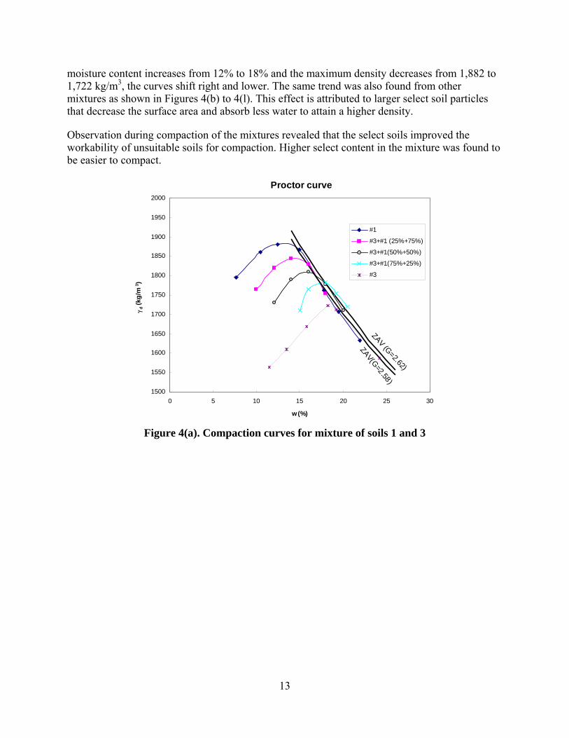
13
moisture content increases from 12% to 18% and the maximum density decreases from 1,882 to 1,722 kg/m3, the curves shift right and lower. The same trend was also found from other mixtures as shown in Figures 4(b) to 4(l). This effect is attributed to larger select soil particles that decrease the surface area and absorb less water to attain a higher density.
Observation during compaction of the mixtures revealed that the select soils improved the workability of unsuitable soils for compaction. Higher select content in the mixture was found to be easier to compact.
Proctor curve
ZAV(G=2.58)
ZAV (G=2.62)
1500
1550
1600
1650
1700
1750
1800
1850
1900
1950
2000
0 5 10 15 20 25 30
w(%)
γ d (k
g/m
3 )
#1
#3+#1 (25%+75%)
#3+#1(50%+50%)
#3+#1(75%+25%)
#3
Figure 4(a). Compaction curves for mixture of soils 1 and 3

14
Proctor curve
ZAV(G=2.58)
ZAV(G=2.7)
1500
1600
1700
1800
1900
2000
2100
2200
0 5 10 15 20 25 30
w(%)
γ d (k
g/m
3 )
#6
#3+#6 (25%+75%)
#3+#6(50%+50%)
#3+#6(75%+25%)
#3
Figure 4(b). Compaction curves for mixture of soils 6 and 3
Proctor curve
ZAV(G=2.58)
ZAV(G=2.69)
1500
1600
1700
1800
1900
2000
2100
0 5 10 15 20 25 30
w(%)
γ d (k
g/m
3 )
#8
#3+#8 (25%+75%)
#3+#8(50%+50%)
#3+#8(75%+25%)
#3
Figure 4(c). Compaction curves for mixture of soils 8 and 3

15
Proctor curve
ZAV(G=2.58)
ZAV(G=2.74)
1500
1550
1600
1650
1700
1750
1800
1850
1900
1950
2000
0 5 10 15 20 25 30
w(%)
γ d (k
g/m
3 )
#9
#3+#9 (25%+75%)
#3+#9(50%+50%)
#3+#9(75%+25%)
#3
Figure 4(d). Compaction curves for mixture of soils 9 and 3
Proctor curve
ZAV(G=2.58)
ZAV(G=2.84)
1500
1600
1700
1800
1900
2000
2100
2200
2300
0 5 10 15 20 25 30
w(%)
γ d (k
g/m
3 )
#10
#3+#10 (25%+75%)
#3+#10(50%+50%)
#3+#10(75%+25%)
#3
Figure 4(e). Compaction curves for mixture of soils 10 and 3

16
Proctor curve
ZAV(G=2.58)
ZAV(G=2.71)
1500
1550
1600
1650
1700
1750
1800
1850
1900
1950
2000
0 5 10 15 20 25 30
w(%)
γ d (k
g/m
3 )
#11
#3+#11 (25%+75%)
#3+#11(50%+50%)
#3+#11(75%+25%)
#3
Figure 4(f). Compaction curves for mixture of soils 11 and 3
Proctor curve
ZAV(G=2.66)ZAV(G=2.62)
1300
1400
1500
1600
1700
1800
1900
2000
2100
0 5 10 15 20 25 30 35
w(%)
γ d (k
g/m
3 )
#1
#12+#1 (25%+75%)
#12+#1(50%+50%)
#12+#1(75%+25%)
#12
Figure 4(g). Compaction curves for mixture of soils 1 and 12

17
Proctor curve
ZAV(G=2.66)
ZAV(G=2.7)
1300
1400
1500
1600
1700
1800
1900
2000
2100
2200
0 5 10 15 20 25 30 35
w(%)
γ d (k
g/m
3 )
#6
#12+#6 (25%+75%)
#12+#6(50%+50%)
#12+#6(75%+25%)
#12
Figure 4(h). Compaction curves for mixture of soils 6 and 12
Proctor curve
ZAV(G=2.66)
ZAV(G=2.69)
1300
1400
1500
1600
1700
1800
1900
2000
2100
0 5 10 15 20 25 30 35
w(%)
γ d (k
g/m
3 )
#8
#12+#8 (25%+75%)
#12+#8(50%+50%)
#12+#8(75%+25%)
#12
Figure 4(i). Compaction curves for mixture of soils 8 and 12

18
Proctor curve
ZAV(G=2.66)
ZAV(G=2.74)
1300
1400
1500
1600
1700
1800
1900
2000
0 5 10 15 20 25 30 35
w(%)
γ d (k
g/m
3 )
#9
#12+#9 (25%+75%)
#12+#9(50%+50%)
#12+#9(75%+25%)
#12
Figure 4(j). Compaction curves for mixture of soils 9 and 12
Proctor curve
ZAV(G=2.66)
ZAV(G=2.84)
1300
1400
1500
1600
1700
1800
1900
2000
2100
2200
2300
0 5 10 15 20 25 30 35
w(%)
γ d (k
g/m
3 )
#10
#12+#10 (25%+75%)
#12+#10(50%+50%)
#12+#10(75%+25%)
#12
Figure 4(k). Compaction curves for mixture of soils 10 and 12

19
Proctor curve
ZAV(G=2.66)
ZAV(G=2.71)
1300
1400
1500
1600
1700
1800
1900
2000
0 5 10 15 20 25 30 35
w(%)
γ d (k
g/m
3 )
#11
#12+#11 (25%+75%)
#12+#11(50%+50%)
#12+#11(75%+25%)
#12
Figure 4(l). Compaction curves for mixture of soils 11 and 12
Maximum Proctor Density and Optimum Moisture Content
Figure 5 presents maximum Proctor density and optimum moisture content for various select-unsuitable mixtures. These figures show that as the proportion of unsuitable soil increases, the maximum dry density decreases and the optimum moisture content increases linearly. These results are attributed to the presence of larger select particles in the soil constituent. The larger select particles decrease the surface area of the soil and absorb less water. The select-unsuitable mixtures with higher content of the select soil exhibit higher values of the maximum dry density. This effect is attributed to the dense packing of soil particles because the workability in performing the compaction is significantly improved for the select-unsuitable mixture with higher amounts of select content.

20
#3+#1
γdmax
wopt
1700
1720
1740
1760
1780
1800
1820
1840
1860
1880
1900
0 20 40 60 80 100
Unsuitable (%)
γ d (k
g/m
3 )
0
2
4
6
8
10
12
14
16
18
20
w (%
)
Figure 5(a). Dry density vs. moisture content for mixture of soils 1 and 3
#3+#6
γdmax
wopt
1700
1750
1800
1850
1900
1950
2000
2050
0 20 40 60 80 100
Unsuitable (%)
γd (k
g/m
3 )
0
2
4
6
8
10
12
14
16
18
20
w(%
)
Figure 5(b). Dry density vs. moisture content for mixture of soils 6 and 3

21
#3+#8
γdmax
wopt
1700
1750
1800
1850
1900
1950
0 20 40 60 80 100
Unsuitable (%)
γd (k
g/m
3 )
0
2
4
6
8
10
12
14
16
18
20
w(%
)
Figure 5(c). Dry density vs. moisture content for mixture of soils 8 and 3
#3+#9
γdmax
wopt
1680
1700
1720
1740
1760
1780
1800
1820
1840
1860
1880
1900
0 20 40 60 80 100
Unsuitable (%)
γd (k
g/m
3 )
0
2
4
6
8
10
12
14
16
18
20
w(%
)
Figure 5(d). Dry density vs. moisture content for mixture of soils 9 and 3

22
#3+#10
γdmax
wopt
1700
1750
1800
1850
1900
1950
2000
2050
0 20 40 60 80 100
Unsuitable (%)
γd (k
g/m
3 )
0
2
4
6
8
10
12
14
16
18
20
w(%
)
Figure 5(e). Dry density vs. moisture content for mixture of soils 10 and 3
#3+#11
γdmax
wopt
1680
1700
1720
1740
1760
1780
1800
1820
1840
1860
1880
0 20 40 60 80 100
Unsuitable (%)
γd (k
g/m
3 )
0
2
4
6
8
10
12
14
16
18
20
w(%
)
Figure 5(f). Dry density vs. moisture content for mixture of soils 11 and 3

23
#12+#1
γdmax
wopt
0
200
400
600
800
1000
1200
1400
1600
1800
2000
0 20 40 60 80 100
Unsuitable (%)
γd (k
g/m
3 )
0
5
10
15
20
25
w(%
)
Figure 5(g). Dry density vs. moisture content for mixture of soils 1 and 12
#12+#6
γdmax
wopt
0
500
1000
1500
2000
2500
0 20 40 60 80 100
Unsuitable (%)
γd (k
g/m
3 )
0
5
10
15
20
25
w(%
)
Figure 5(h). Dry density vs. moisture content for mixture of soils 6 and 12

24
#12+#8
γdmax
wopt
0
500
1000
1500
2000
2500
0 20 40 60 80 100
Unsuitable (%)
γd (k
g/m
3 )
0
5
10
15
20
25
w(%
)
Figure 5(i). Dry density vs. moisture content for mixture of soils 8 and 12
#12+#9
γdmax
wopt
0
200
400
600
800
1000
1200
1400
1600
1800
2000
0 20 40 60 80 100
Unsuitable (%)
γ d (k
g/m
3 )
0
5
10
15
20
25
w(%
)
Figure 5(j). Dry density vs. moisture content for mixture of soils 9 and 12

25
#12+#10
γdmax
wopt
0
500
1000
1500
2000
2500
0 20 40 60 80 100
Unsuitable (%)
γd (k
g/m
3 )
0
5
10
15
20
25
w(%
)
Figure 5(k). Dry density vs. moisture content for mixture of soils 10 and 12
#12+#11
γdmax
wopt
0
200
400
600
800
1000
1200
1400
1600
1800
2000
0 20 40 60 80 100
Unsuitable (%)
γ d (k
g/m
3 )
0
5
10
15
20
25
w(%
)
Figure 5(l). Dry density vs. moisture content for mixture of soils 11 and 12

26
Blotz et al. (1998) developed an empirical method to estimate maximum dry density (γdmax) and optimum moisture (wopt) content of compacted clays from liquid limit (LL). It was found a linear relationship exists between γdmax, wopt, and LL at any compactive effort. Figure 6 presents the relationship between optimum moisture content and maximum dry density of all mixtures. The compactive effort used for each sample was equal. A trend line is added to the data points and it shows that maximum density decreases linearly with increasing optimum moisture content, with R2 of 0.93. The relationship between maximum Proctor density (γdmax) and optimum moisture content (wopt) can be expressed by:
γdmax (kg/m3) = -39.961 wopt +2410.7 (1)
y = -39.961x + 2410.7R2 = 0.9321
1450
1550
1650
1750
1850
1950
2050
10 15 20 25
Optimum MC (%)
Proc
tor d
ensi
ty (k
g/m
3 )
Figure 6. Relationship of proctor density and optimum moisture content
Strength of Mixtures
Figure 7 presents unconfined compression strength results at different moisture contents for each select-unsuitable mixture. When the moisture content is high, soil is very soft. From Figure 7(j), it can be seen that at moisture contents as high as 33%, soil no. 12 has an unconfined compression strength of 23 kPa. This compression strength is the lowest strength of all soils including mixtures and occurs at a compressive strain of 16%. While the maximum unconfined compression strength of these mixtures is 651 kPa, which is the strength of soil no. 9 at 10% moisture content, this soil is very strong and brittle fails at a compressive strain as low as 5%. Figure 7 shows a trend that as the moisture content increases, unconfined compression strength decreases. However, at very dry conditions (w% < 10%), the unconfined compression strength

27
may increase with increasing moisture content. From Figure 7, it can also be seen that the maximum unconfined compression strength occurs at moisture content less than optimum moisture content of Proctor compaction. For example, Figure 7(a) shows that soil no. 1 has maximum unconfined compression strength of 531 kPa at 10% moisture content, which is less than 12% optimum moisture content.
0
100
200
300
400
500
600
0 5 10 15 20 25 30
w(%)
qu (k
Pa)
#1
#3+#1 (25%+75%)
#3+#1(50%+50%)
#3+#1(75%+25%)
#3
Figure 7(a). UCS vs. moisture content for mixture soils 1 and 3
0
100
200
300
400
500
600
0 5 10 15 20 25 30
w(%)
qu (k
Pa)
#6
#3+#6 (25%+75%)
#3+#6(50%+50%)
#3+#6(75%+25%)
#3
Figure 7(b). UCS vs. moisture content for mixture soils 6 and 3

28
0
100
200
300
400
500
600
0 5 10 15 20 25 30
w(%)
qu (k
Pa)
#8
#3+#8 (25%+75%)
#3+#8(50%+50%)
#3+#8(75%+25%)
#3
Figure 7(c). UCS vs. moisture content for mixture soils 8 and 3
0
100
200
300
400
500
600
700
0 5 10 15 20 25 30
w(%)
qu (k
Pa)
#9
#3+#9 (25%+75%)
#3+#9(50%+50%)
#3+#9(75%+25%)
#3
Figure 7(d). UCS vs. moisture content for mixture soils 9 and 3

29
0
100
200
300
400
500
600
700
0 5 10 15 20 25 30
w(%)
qu (k
Pa)
#10
#3+#10 (25%+75%)
#3+#10(50%+50%)
#3+#10(75%+25%)
#3
Figure 7(e). UCS vs. moisture content for mixture soils 10 and 3
0
100
200
300
400
500
600
0 5 10 15 20 25 30
w(%)
qu (k
Pa)
#11
#3+#11 (25%+75%)
#3+#11(50%+50%)
#3+#11(75%+25%)
#3
Figure 7(f). UCS vs. moisture content for mixture soils 11 and 3

30
0
100
200
300
400
500
600
0 5 10 15 20 25 30 35
w(%)
qu (k
Pa)
#1
#12+#1 (25%+75%)
#12+#1(50%+50%)
#12+#1(75%+25%)
#12
Figure 7(g). UCS vs. moisture content for mixture soils 1 and 12
0
100
200
300
400
500
600
0 5 10 15 20 25 30 35
w(%)
qu (k
Pa)
#6
#12+#6 (25%+75%)
#12+#6(50%+50%)
#12+#6(75%+25%)
#12
Figure 7(h). UCS vs. moisture content for mixture soils 6 and 12

31
0
100
200
300
400
500
600
0 5 10 15 20 25 30 35
w(%)
qu (k
Pa)
#8
#12+#8 (25%+75%)
#12+#8(50%+50%)
#12+#8(75%+25%)
#12
Figure 7(i). UCS vs. moisture content for mixture soils 8 and 12
0
100
200
300
400
500
600
700
0 5 10 15 20 25 30 35
w(%)
qu (k
Pa)
#9
#12+#9 (25%+75%)
#12+#9(50%+50%)
#12+#9(75%+25%)
#12
Figure 7(j). UCS vs. moisture content for mixture soils 9 and 12

32
0
100
200
300
400
500
600
700
0 5 10 15 20 25 30 35
w(%)
qu (k
Pa)
#10
#12+#10 (25%+75%)
#12+#10(50%+50%)
#12+#10(75%+25%)
#12
Figure 7(k). UCS vs. moisture content for mixture soils 10 and 12
0
100
200
300
400
500
600
0 5 10 15 20 25 30 35
w(%)
qu (k
Pa)
#11
#12+#11 (25%+75%)
#12+#11(50%+50%)
#12+#11(75%+25%)
#12
Figure 7(l). UCS vs. moisture content for mixture soils 11 and 12
Classification of Mixtures
Table 4 summarizes the index properties, compaction test results, unconfined compression test results, and classification of all mixtures. From the table, it can be seen that some of the mixtures still can be classified as select soil when the proportion of unsuitable is low (25% unsuitable). When percent unsuitable is as high as 75%, the mixture is either a suitable or an unsuitable soil. All the mixtures are poorer materials than select soil alone. However, to reduce the cost of

33
construction, it is recommended that a mixture of select-unsuitable soils at a ratio of 3:1 be used as the top 0.6 m of subgrade.
General Mixing Conclusions and Recommendations
Improving the properties of unsuitable soils by mixing them with select soils were evaluated at various proportions of select-unsuitable soil mixtures: 0%:100%, 25%:75%, 50%:50%, and 100%:0%. Several conclusions were drawn from the results of this phase of the study.
1. The Atterberg limits variation of these soils is very small, with liquid limit and plasticity index ranging from 25 to 41 and 10 to 21, respectively. It is hard to see how the Atterberg limits change as percent unsuitable is increased. It is recommended that more unsuitable soils with high plasticity and more granular select soils be collected in the future research.
2. Experimental results indicate that maximum dry density and unconfined compression strength both increase while the optimum moisture content decreases linearly with increasing select proportion. The maximum dry density decreases linearly with increasing optimum moisture content.
3. When moisture content is greater than about 10%, unconfined compression strength decreases with increasing moisture content. When moisture content is less than 10%, however, the soil is brittle and may have a higher strength at higher moisture content.
4. The select-unsuitable mixture is a poorer material than select soil alone. However, from the test results, a 75% select and 25% unsuitable mixture can still be classified as a select soil. To reduce the cost of construction, a mixture of select-unsuitable soils at a ratio of 3:1 can still be used as the top 0.6 m of subgrade.

Tab
le 4
(a).
Sum
mar
y of
pro
pert
ies o
f sel
ect-
unsu
itabl
e (u
nsui
tabl
e so
il no
. 12)
mix
ture
s
Mix
ed so
il LL
PL
PI
%
G
rave
l %
Sa
nd
%
Silt
%
Cla
y Pr
octo
r de
nsity
O
ptim
um
w%
G
I EP
C
clas
sific
atio
n G
s qu
(k
Pa)
E50
(k
Pa)
%
Uns
uita
ble
6 26
13
13
1
46
37
17
2030
10
4
Sele
ct
2.70
35
6 99
00
0 12
&6(
25%
+75%
) 30
14
16
1
36
50
13
1866
15
7
Sele
ct
2.69
41
1 13
733
25
12&
6(50
%+5
0%)
33
18
15
1 25
63
11
17
72
15
10
Sele
ct
2.68
31
6 79
00
50
12&
6(75
%+2
5%)
37
20
17
0 15
75
10
15
91
19
14
Suita
ble
2.67
20
9 59
43
75
12
41
29
12
0 4
88
9 14
95
22
14
Uns
uita
ble
2.66
18
7 58
13
100
1 35
18
17
11
25
45
19
18
82
12
9 Se
lect
2.
62
429
9350
0
12&
1(25
%+7
5%)
37
19
18
8 20
56
16
18
33
15
11
Sele
ct
2.63
39
0 97
50
25
12&
1(50
%+5
0%)
37
23
14
6 14
67
14
17
33
17
11
Suita
ble
2.64
34
1 89
47
50
12&
1(75
%+2
5%)
39
24
15
3 9
77
11
1629
18
14
Su
itabl
e 2.
65
325
1012
5 75
12
41
29
12
0
4 88
9
1495
22
14
U
nsui
tabl
e 2.
66
187
5813
10
0 8
35
19
16
3 27
56
14
19
38
12
9 Se
lect
2.
69
336
1050
0 0
12&
8(25
%+7
5%)
37
21
16
2 21
64
13
18
30
14
11
Sele
ct
2.68
29
0 91
20
25
12&
8(50
%+5
0%)
38
24
14
2 15
72
11
17
30
17
12
Suita
ble
2.68
25
4 83
40
50
12&
8(75
%+2
5%)
39
25
14
1 9
80
10
1603
20
14
U
nsui
tabl
e 2.
67
210
7855
75
12
41
29
12
0
4 88
9
1495
22
14
U
nsui
tabl
e 2.
66
187
5813
10
0 9
34
18
16
5 29
56
10
18
87
13
8 Se
lect
2.
74
561
1873
0 0
12&
9(25
%+7
5%)
35
19
16
4 23
64
10
17
90
15
10
Sele
ct
2.72
46
8 16
220
25
12&
9(50
%+5
0%)
38
23
15
3 16
72
9
1675
17
12
Su
itabl
e 2.
70
378
1310
0 50
12
&9(
75%
+25%
) 39
24
15
1
10
80
9 16
50
19
14
Suita
ble
2.68
30
0 84
00
75
12
41
29
12
0 4
88
9 14
95
22
14
Uns
uita
ble
2.66
18
7 58
13
100
10
25
16
10
2 44
40
14
19
97
11
2 Se
lect
2.
84
507
1814
0 0
12&
10(2
5%+7
5%)
29
16
14
2 34
52
13
18
89
13
6 Su
itabl
e 2.
80
429
1592
6 25
12
&10
(50%
+50%
) 34
21
13
1
24
64
11
1761
17
9
Uns
uita
ble
2.75
32
1 80
50
50
12&
10(7
5%+2
5%)
37
25
13
1 14
76
10
16
42
19
11
Uns
uita
ble
2.71
32
9 10
312
75
12
41
29
12
0 4
88
9 14
95
22
14
Uns
uita
ble
2.66
18
7 58
13
100
11
33
18
15
3 31
45
21
18
57
14
7 Se
lect
2.
71
444
1306
0 0
12&
11(2
5%+7
5%)
34
18
16
2 24
56
18
17
68
15
10
Sele
ct
2.70
43
4 12
400
25
12&
11(5
0%+5
0%)
37
21
16
2 17
67
15
16
82
17
12
Suita
ble
2.69
36
5 11
375
50
12&
11(7
5%+2
5%)
38
24
14
1 10
77
12
15
93
20
13
Suita
ble
2.67
23
6 53
64
75
12
41
29
12
0 4
88
9 14
95
22
14
Uns
uita
ble
2.66
18
7 58
13
100
34

Tab
le 4
(b).
Sum
mar
y of
pro
pert
ies o
f sel
ect-
unsu
itabl
e (u
nsui
tabl
e so
il no
. 3) m
ixtu
res
2 39
18
21
0
1 81
18
17
46
17
21
Suita
ble
2.67
34
1 94
44
0 3&
2(25
%+7
5%)
35
22
13
0 1
83
16
1742
17
14
U
nsui
tabl
e 2.
65
303
7550
25
3&
2(50
%+5
0%)
37
26
11
0 1
85
15
1720
17
13
U
nsui
tabl
e 2.
63
315
9813
50
3&
2(75
%+2
5%)
34
24
10
0 0
86
14
1689
18
12
U
nsui
tabl
e 2.
60
252
7412
75
3
34
22
12
0 0
88
12
1730
19
13
U
nsui
tabl
e 2.
58
302
7500
10
0 11
33
18
15
3
31
45
21
1857
14
7
Sele
ct
2.71
44
4 13
060
0 3&
11(2
5%+7
5%)
34
17
17
2 23
56
18
18
09
15
11
Sele
ct
2.68
34
9 95
11
25
3&11
(50%
+50%
) 35
19
16
2
15
67
16
1770
17
12
Su
itabl
e 2.
65
265
7389
50
3&
11(7
5%+2
5%)
34
20
14
1 8
77
14
1696
17
13
U
nsui
tabl
e 2.
61
260
9286
75
3
34
22
12
0 0
88
12
1730
19
13
U
nsui
tabl
e 2.
58
302
7500
10
0 10
25
16
10
2
44
40
14
1997
11
2
Sele
ct
2.84
50
7 18
140
0 3&
10(2
5%+7
5%)
27
17
10
2 33
52
14
19
28
12
4 Su
itabl
e 2.
78
409
1360
0 25
3&
10(5
0%+5
0%)
29
16
13
1 22
64
13
18
18
15
8 U
nsui
tabl
e 2.
71
301
8780
50
3&
10(7
5%+2
5%)
32
19
13
1 11
76
13
17
24
18
11
Uns
uita
ble
2.65
22
6 60
11
75
3 34
22
12
0
0 88
12
17
30
19
13
Uns
uita
ble
2.58
30
2 75
00
100
9 34
18
16
5
29
56
10
1887
13
8
Sele
ct
2.74
56
1 18
730
0 3&
9(25
%+7
5%)
33
19
14
4 22
64
11
18
87
12
9 Su
itabl
e 2.
70
454
1816
0 25
3&
9(50
%+5
0%)
35
19
16
3 15
72
11
18
07
15
12
Suita
ble
2.66
31
2 10
540
50
3&9(
75%
+25%
) 34
17
17
1
7 80
12
17
08
17
15
Suita
ble
2.62
23
0 66
86
75
3 34
22
12
0
0 88
12
17
30
19
13
Uns
uita
ble
2.58
30
2 75
00
100
6 26
13
13
1
46
37
17
2030
10
4
Sele
ct
2.70
35
6 99
00
0 3&
6(25
%+7
5%)
28
15
13
0 34
50
15
19
53
13
6 Su
itabl
e 2.
67
435
1644
0 25
3&
6(50
%+5
0%)
31
17
14
0 23
63
14
18
52
15
9 U
nsui
tabl
e 2.
64
325
9205
50
3&
6(75
%+2
5%)
34
20
14
0 11
75
13
18
00
17
12
Uns
uita
ble
2.61
31
0 78
90
75
3 34
22
12
0
0 88
12
17
30
19
13
Uns
uita
ble
2.58
30
2 75
00
100
1 35
18
17
11
25
45
19
18
82
12
9 Se
lect
2.
62
429
9350
0
3&1(
25%
+75%
) 34
18
16
8
19
56
17
1844
14
10
Se
lect
2.
61
380
8890
25
3&
1(50
%+5
0%)
30
17
13
6 13
67
16
18
10
16
9 U
nsui
tabl
e 2.
60
360
8630
50
3&
1(75
%+2
5%)
35
24
11
3 6
77
14
1782
18
11
U
nsui
tabl
e 2.
59
345
7980
75
3
34
22
12
0 0
88
12
1730
19
13
U
nsui
tabl
e 2.
58
302
7500
10
0 8
35
19
16
3 27
56
14
19
38
12
9 Se
lect
2.
69
336
1050
0 0
3&8(
25%
+75%
) 34
18
16
2
20
64
14
1888
14
11
Se
lect
2.
66
330
9730
25
3&
8(50
%+5
0%)
33
17
16
2 13
72
13
18
25
16
12
Suita
ble
2.64
31
5 88
10
50
3&8(
75%
+25%
) 36
21
15
1
7 80
13
17
70
18
14
Suita
ble
2.61
32
0 94
30
75
3 34
22
12
0
0 88
12
17
30
19
13
Uns
uita
ble
2.58
30
2 75
00
100
35

36
Site-Specific Example: Fairfield Bypass, Jefferson County
Presently, when soils are deemed unsuitable for a particular engineering purpose (e.g., fill, subgrade), the soils can be removed and wasted or the soils’ engineering properties can be improved through mechanical compaction or chemical stabilization. When a project site has a considerable amount of unsuitable soils, it becomes costly to have to waste all the unsuitable materials. Additionally, borrowing materials from other sources may prove to be more expensive than using local available materials (Winterkorn et al. 1991). Some soils are not amenable to sufficient improvement using compaction alone. Chemical stabilization of soils is accomplished by mixing them with various chemicals, such as cement, lime, and fly ash. It has been shown that mixing soils with these chemicals can improve certain properties of soil to make the soil serve adequately an intended engineering purpose. For example, a soil-cement mixture can reduce the volume change tendency and plasticity and increase load-bearing capacity of the soil. However, high plasticity clays require larger amount of cements, which may not be economically viable. The liquid limit, plasiticity index, and percent passing No. 200 sieve generally are limited to 40%, 18%, and 35%, respectively (Winterkorn et al. 1991). In recent years, natural poor soils mixed with granular materials are also used in construction of base, subbase, and surface courses of paved facilities. Leelani (1989) studied the properties of an existing active clay by adding various proportions of a fine sand and found that a 20% sand admixture can improve the properties of the active clay adequately for highway embankment construction. Granular stabilization can obtain a well-proportioned mixture of particles with continuous gradation (well-graded) and the desired plasticity. The granular constituents form a bearing skeleton, while fine portions can provide effective cohesion and cementation. However, generally, the natural soils will lack some constituents needed to form a continuous bearing skeleton or to provide the necessary cohesion and cementation. In these cases, the desired blend can be compounded by adding proper proportions of the granular materials or fines (Winterkorn et al. 1991). One method to optimize and manage these available materials is to selectively mix the on-site soils—for example, mixing select soils with unsuitable soils. In the field, the blending of soils is accomplished by a pulvamixer or equivalent. Figure 8 shows a Multi-Terrain Mixer generally used for soil mixing (Gutzwiller 2006). The mix should be prewetted to specified moisture content and thoroughly mixed by a mixer to a homogeneous, friable mixture that is free from all clods or lumps. Compaction begins immediately after the mixing is completed. The mixtures are compacted layer by layer to the specified density until the required elevation is attained. Compaction is achieved using a vibratory padfoot roller for granular materials and sheepsfoot roller for cohesive soils.
The soils used in this study were from a proposed bypass for Highway 34 around the city of Fairfield, Jefferson County, Iowa. The proposed bypass was approximately 10 miles in length and consisted of numerous cuts and fills some 5 to 6 meters in height. The soils along the route consisted of clay pan, loess, paleosol (gumbotil), and Kansan glacial till layer (NRCS 1992). The clay pan and gumbotil have high swell potential, while the loess is potentially collapsible, resulting in unsuitable ratings for these soils. The glacial till layer was classified as a select soil. Due to the large amount of unsuitable soils along the route, the potential for soil mixing of select and unsuitable soil for improving the unsuitable soil was studied.

37
Figure 8. Type MGM 250 soil mixer (Gutzwiller 2006)
This section presents how the engineering properties (such as plasticity index, unconfined compressive strength, compaction characteristics, etc.) of select-unsuitable blends change with various mixing proportions. Based on the test results, recommendations of proportions of select-unsuitable blends are provided.
Site-Specific Materials
Soils were collected from the site using a drill rig down to a depth of 5.7 m. Bag samples of each soil layer were collected from the auger, as well as three-inch Shelby tube samples. Based on the texture and color of the soils, the soil profile was divided into four layers, 0 to 1.5 m (clay pan), 1.5 to 2.7 m (loess), 2.7 to 4.2 m (weathered gumbotil), and 4.2 to 5.7 m (sandy Kansan glacial till) and named soil no. 1 to no. 4, respectively.
Laboratory gradation tests, Atterberg limits, compaction, and unconfined compression strength tests were performed on the four soils in two series. In the first series, these tests are conducted to classify the four soils into select, suitable, and unsuitable. In the second series, the same tests were conducted on select-unsuitable blends at various proportions.
Gradation tests were conducted in accordance to ASTM D 2487 “Standard Practice for Classification of Soils for Engineering Purposes” (ASTM 2003). Atterberg limits tests were performed according to ASTM D 4318 “Standard Test Methods for Liquid Limit, Plastic Limit, and Plasticity Index of Soils” (ASTM 2003). For the mixtures, select soils passing through the No. 40 sieve were mixed with unsuitable soils passing through the No. 40 sieve at various proportions.
Compaction tests were performed on 2 x 2 in. cylindrical samples in accordance with O’Flaherty et al. (1963). A standard Proctor compaction sample is made in a 1/30 ft3 cylinder mold using three layers that are each compacted by 25 blows of the 5.5 lb rammer dropped 12 inches for an energy input of 12,375 ft-lb/ft3. Another test, the ISU 2 x 2 in. compaction test method, utilizes specimens 2 inches in diameter by 2 inches high that are compacted by 10 blows of the 5 lb

38
hammer dropped 12 inches for an energy input of 13,751 ft-lb/ft3, which requires only about one-tenth of the material and one-third of the time needed for standard Proctor specimens. However, the maximum dry density and optimum moisture content obtained from the two test methods are very close. O’Flaherty et al. (1963) have shown that the ISU 2 x 2 in. compaction apparatus can be used in lieu of the standard Proctor compaction test to increase productivity.
Unconfined compression strength tests were performed on 2 x 4 in. cylindrical samples at different moisture contents in accordance with ASTM D 2166-00 “Test Method for Unconfined Compressive Strength of Cohesive Soil” (ASTM 2003). Soil was put in two layers and the compaction energy was doubled compared to 2 x 2 in. samples.
For the compaction and unconfined compression test samples, air-dried select soils passing through a No. 4 sieve were mixed with unsuitable soils passing through a No. 4 sieve at various proportions. The required weight of the soil was determined based on the dry unit weight, water content, and the volume of the specimen. The required amount of water was added to the dry soil and thoroughly mixed. The blends were allowed to hydrate for 24 hours prior to testing.
Site-Specific Results and Discussion
In Situ and Mixed Soils
The full-depth profiles of soil index properties and classifications are summarized in Table 5. Figure 9 shows the grain size distribution of the four soils. As indicated in Table 5 and Figure 9, the fines contents decrease from 98% of the top layer (0 to 1.5 m) to 64% of the bottom layer (4.2 to 5.7 m). Soils no. 1 and 3 are fat clays and potentially expansive, and their liquid limit and plasticity index are much higher than those of the other two layers. Soils no. 1 and 3 are classified as CH (A-7-5), while soils no. 2 and 4 are classified as CL (A-6). Compaction test results indicate that soils no. 1 and 3 have relatively high optimum moisture contents and low dry densities compared to soils no. 2 and 4. Soils no. 1 and 3 are weaker soils, as indicated by high Group Index (GI) and low unconfined compressive strength. According to Iowa DOT classification, soils no. 1, 2, and 3 are classified as unsuitable soils, while no. 4 is classified as select soil. The select soil contains considerably more sand than the three unsuitable soils.
To determine the amount of mixing to be used in the field, the physical and engineering properties of different mixes were investigated. In this test program, the select soil (no. 4) was mixed with each unsuitable soil (no. 1, 2, and 3) at 75:25, 50:50, and 25:75 proportions. The engineering properties are summarized in Table 6.

Tab
le 5
. Sum
mar
y of
pro
pert
ies o
f sel
ect a
nd u
nsui
tabl
e so
ils
Soil
Dep
th
(m)
LL
PL
PI
%
Gra
vel
%
Sand
%
Si
lt %
C
lay
Proc
tor
dens
ity
(kg/
m3 )
Opt
imum
w
%
Gro
up
inde
x G
I q u
(k
Pa)
USC
S /A
SSH
TOID
OT
clas
sific
atio
n1
(cla
y pa
n)
0-1.
5
53
27
26
0
2
58
40
1716
19
.0
30
376
C
H/A
-7-6
Uns
uita
ble
2 (lo
ess)
1.
5-2.
7
30.6
18
.4
12.2
0
9
64
27
18
56
14.0
10
36
6
CL/
A-6
U
nsui
tabl
e
3 (g
umbo
) 2.
7-4.
2 58
.5
25.9
32
.6
0
11
43
46
1668
21
.0
32
295
C
H/A
-7-6
Uns
uita
ble
4 (g
laci
al ti
ll)
4.2-
5.7
39
17
.4
21.6
0
36
34
30
19
12
13.0
11
40
6
CL/
A-6
Se
lect
Not
e: q
u was
mea
sure
d at
opt
imum
moi
stur
e co
nten
t. U
: Uns
uita
ble,
S: S
elec
t.
Tab
le 6
. Sum
mar
y of
pro
pert
ies o
f sel
ect a
nd u
nsui
tabl
e bl
ends
So
il B
lend
U:S
LL
PL
PI
%
G
rave
l%
Sa
nd
%
Silt
%
Cla
y
Proc
tor
dens
ity
(kg/
m3 )
Opt
imum
w
%
Gro
up
inde
x G
I q u
(k
Pa)
USC
S /A
SSH
TOID
OT
clas
sific
atio
n
75:2
5 47
23
24
0
10
52
38
17
65
17.5
23
37
1
CL/
A-7
-6Su
itabl
e
1 an
d 4
50:5
0 44
22
22
0
19
46
35
18
16
15.7
18
38
1
CL/
A-7
-6Su
itabl
e
25:7
5 40
19
21
0
27
40
33
18
61
14.1
14
39
3
CL/
A-6
Se
lect
75
:25
33
19.5
13
.5
0
15
57
28
1861
14
.1
11
369
CL/
A-6
U
nsui
tabl
e
2 an
d 4
50:5
0 34
.5
17.1
17
.4
0
22
49
29
1866
13
.7
12
375
CL/
A-6
Su
itabl
e
25:7
5 37
18
19
0
29
42
29
18
93
13.2
12
39
0 C
L/A
-6
Sele
ct
75
:25
48
24
24
0
17
41
42
1693
19
.2
21
401
CL/
A-7
-6Su
itabl
e
3 an
d 4
50:5
0 45
.4
22.5
22
.9
0
23
39
38
1747
17
.3
17
359
CL/
A-7
-6Su
itabl
e
25:7
5 40
21
20
0
29
37
34
18
19
15.5
13
40
0 C
L/A
-6
Sele
ct
Not
e: q
u was
mea
sure
d at
opt
imum
moi
stur
e co
nten
t. U
: Uns
uita
ble,
S: S
elec
t.
39

40
Gravel Sand ClaySilt
0
10
20
30
40
50
60
70
80
90
100
0.00010.0010.010.1110
Particle diameter(mm)
Perc
ent f
iner
(%)
#1(Unsuitable)#2 (Unsuitable)
#3 (Unsuitable)#4 (Select)
Figure 9. Grain size distribution of select and unsuitable soils
Index Properties of Mixtures
Index properties of all the mixed soils were determined at the various blends. The Casagrande plasticity chart for all the soils and blends at various proportions is shown in Figure 10. As can be seen in the figure, all the blends are located in the CL zone (low/medium plasticity to medium plasticity) and between the endpoints of individual select and unsuitable soils. As the select proportion increases, the liquid limit and plasticity index of the blends move closer to those of the select soil. Mixing with select soil reduces the plasticity and swelling potential dramatically, especially for blends of no. 4 mixed with no. 3.

41
"U" L
ine: PI
=0.9(
LL-8)
"A" L
ine: PI=
Note:S=Select, U=UnsuitableMixing Proportion: S:U4 CL-ML
CL or O
L
ML or OL
0.73(LL-20
)
7
CH or O
H
MH or OH
#3(U)
#1(U)
#4(S)
#2 (U)
1:31:1
3:1
1:3
1:13:1
3:11:1
1:3
0
10
20
30
40
50
60
0 10 20 30 40 50 60 70 80 90 100Liquid Limit, LL (%)
Plas
ticity
Inde
x, P
I (%
)Individual soilBlend 3&4Blend 1&4Blend 2&4
Figure 10. Casagrande plasticity chart of select, unsuitable, and blends
Compaction Characteristics
Figure 11 shows the Proctor curves of the four in situ soils. From this figure, it can be seen that soils no. 1 and 3 have much lower dry unit weights than the select soil, indicative of their higher plasticity. Soil no. 2 has a compaction curve very similar to the select soil (no. 4). Figure 12 presents the spectrum of Proctor density curves at five mix proportions. Each density curve in Figure 12 represents the variation of dry unit weight with moisture content at a specified ratio of the select-unsuitable blend. At least five samples were prepared at different moisture contents for each compaction curve. The zero-air line is also plotted in Figure 12. The uppermost curve in Figure 12(a) is the result of the compaction test from no. 4, which is a select soil (proportion of select:unsuitable = 100%:0%), while the lowermost curve represents the density curve for unsuitable soil no. 1 (proportion of select:unsuitable = 0%:100%). It indicates that select soil alone has highest value of dry density at the lowest value of moisture content. As the percent of unsuitable increases in the mixture, optimum moisture content increases from 13% to 19%, maximum density decreases from 1,912 to 1,716 kg/m3, and the curves shift right and below. The same trend was also found from other blends, as shown in Figures 12(b) and 12(c). This effect is attributed to larger select soil particles that decrease the surface area and absorb less water to attain a higher density. The line of optimum in Figure 12 is approximately linear, which indicates a linear relationship exists between maximum dry density/optimum moisture content and mixing proportion.

42
Observations during the compaction tests indicate that the select soils improved the workability of unsuitable soils for compaction. Higher select content in the mixture was found to be easier to compact.
ZAV (Gs = 2.65)
1500
1600
1700
1800
1900
2000
5 10 15 20 25 30
Moisture Content (%)
Dry
Uni
t Wei
ght (
kg/m
3 )
94
99
104
109
114
119
124
Dry
Uni
t Wei
ght (
pcf)
#1(Unsuitable)
#2 Unsuitable
#3 Unsuitable
#4 Select
ZAV
Figure 11. Compaction curves of soil no. 1, no. 2, no. 3, and no. 4
ZAV (Gs = 2.65)
Line of Opt.
1500
1600
1700
1800
1900
2000
5 10 15 20 25 30Moisture Content (%)
Dry
Uni
t Wei
ght (
kg/m
3 )
94
99
104
109
114
119
124
Dry
Uni
t Wei
ght (
pcf)
#1(Unsuitable)#1+#4 (75%+25%)#1+#4(50%+50%)#1+#4(25%+75%)#4(Select)ZAVLine of Opt.
Figure 12(a). Compaction curves of no. 4 and no. 1 blends

43
ZAV (Gs = 2.65)
Line of Opt.
1700
1800
1900
2000
5 10 15 20 25 30Moisture Content (%)
Dry
Uni
t Wei
ght (
kg/m
3 )
106
108
110
112
114
116
118
120
122
124
Dry
Uni
t Wei
ght (
pcf)
#2(Unsuitable)
#2+#4 (75%+25%)
#2+#4(50%+50%)
#2+#4(25%+75%)
#4(Select)
ZAV
Line of Opt.
Figure 12(b). Compaction curves of no. 4 and no. 2 blends
ZAV (Gs = 2.65)
Line of Opt.
1500
1600
1700
1800
1900
2000
5 10 15 20 25 30
Moisture Content (%)
Dry
Uni
t Wei
ght (
kg/m
3 )
94
99
104
109
114
119
124
Dry
Uni
t Wei
ght (
pcf)
#3(Unsuitable)
#3+#4 (75%+25%)
#3+#4(50%+50%)
#3+#4(25%+75%)
#4(Select)
ZAV
Line of Opt.
Figure 12(c). Compaction curves of no. 4 and no. 3 blends

44
Maximum Proctor Density and Optimum Moisture Content
Blotz et al. (1998) developed an empirical method to estimate maximum dry density (γdmax) and optimum moisture (wopt) content of compacted clays from liquid limit (LL). It was found a linear relationship exists between γdmax, wopt, and LL at any compactive effort. Figure 13 presents the relationship between optimum moisture content and maximum dry density of all blends. A trend line is added to the data points and shows that maximum density decreases linearly with increasing optimum moisture content, with an R2 of 0.98. The relationship between maximum Proctor density (γdmax) and optimum moisture content (wopt) can be expressed by:
γdmax (kg/m3) = -30.284 wopt +2288.5 (2)
y = -30.284x + 2288.5R2 = 0.9836
1600
1650
1700
1750
1800
1850
1900
1950
0 5 10 15 20 25
Optimum Moisture Content w (%)
Proc
tor D
ensi
ty (k
g/m
3 )
Figure 13. Maximum dry density vs. optimum moisture content
Strength of Mixture
Figure 14 presents unconfined compression strength (UCS) vs. moisture content for each select-unsuitable blend. The unconfined compression strength ranges from 100 kPa to 555 kPa and decreases with increasing moisture content even as the dry density increases. The peak strength occurs at approximately 2% to 5% dry of optimum. Meanwhile, at a specified moisture content w%, when the select proportion increases, the UCS of the blend increases. The UCS of the select soil and that of the unsuitable soil are at the endpoints of the spectrum. From Figure 14 the UCS of the blend can be determined by mixing proportion and compaction moisture content.

45
Line of Optimum
0
100
200
300
400
500
600
5 10 15 20 25
Moisture Content (%)
Unc
onfin
ed C
ompr
essi
on S
tren
gth
qu
(kPa
)#4(Select)
#1+#4(25%+75%)
#1+#4(50%+50%)
#1+#4(75%+25%)
#1(Unsuitable)
Opt w %
Figure 14(a). UCS of no. 4 and no. 1 blends
Line of Optimum
0
100
200
300
400
500
600
5 10 15 20
Moisture Content (%)
Unc
onfin
ed C
ompr
essi
on S
treng
th q
u (kP
a)
#4(Select)
#2+#4(25%+75%)
#2+#4(50%+50%)
#2+#4(75%+25%)
#2(Unsuitable)
Opt w %
Figure 14(b). UCS of no. 4 and no. 2 blends

46
Line of Optimum
0
100
200
300
400
500
600
5 10 15 20 25 30Moisture Content (%)
Unc
onfin
ed C
ompr
essi
on S
treng
th q
u (kP
a)
#4(Select)
#3+#4(25%+75%)
#3+#4(50%+50%)
#3+#4(75%+25%)
#3(Unsuitable)
Opt w%
Figure 14(c). UCS of no. 4 and no. 3 blends
Classification of Blends
Table 6 summarizes the index properties, compaction test results, unconfined compression test results, and classification of all blends. From the table, it can be seen that some of the mixtures can still be classified as select soil when the proportion of unsuitable is low (25% unsuitable). Using 50:50 mixtures results in a suitable soil classification for the soils tested in this study. When the percent unsuitable is as high as 75%, the mixture is either a suitable soil or an unsuitable soil. Only in the case of soil no. 2, the loess, does the mixture result in an unsuitable classification. All the mixtures are poorer materials than select soil alone. These results provide a means of extending the use of on-site soils using soil mixing. Based on the results shown, 50:50 blends and 25:75 unsuitable to suitable soil blends provide acceptable soils for most purposes. Thus, rather than wasting site soils that are deemed unsuitable, the soils can be used in conjunction with select soils to increase the use of on-site soils and decrease the amount of off-site borrow.
Site-Specific Conclusions and Recommendations
Improving the properties of unsuitable soils by mixing them with select soils were evaluated at various proportions of select-unsuitable soil mixtures: 0%:100%, 25%:75%, 50%:50%, and 100%:0%. Several conclusions were drawn from the results of this study.
1. Mixing with select soil can improve the index properties of unsuitable soil by reducing the liquid limit and plasticity index.
2. Experimental results indicate that maximum dry density and UCS both increase while the optimum moisture content decreases linearly with increasing select proportion.
3. The UCS of the select-unsuitable blends decreases with increasing moisture content.

47
4. Select blends can be obtained by mixing up to 25% of an unsuitable soil with 75% select soil.
5. Suitable blends can be obtained by mixing 50% of unsuitable soil with 50% of select soil.
6. At 75% unsuitable with 25% select, some soils will be classified as suitable and some as unsuitable.
7. For the soils tested in this study, the addition of unsuitable soils to a select soil in the range of 25 to 50% provides acceptable soils for placement in embankment applications.

48
SATURATED PERMEABILITY OF COMPACTED GLACIAL TILL IN IOWA
Introduction
The performance of a pavement structure is dependent upon the stability and deformation resistance of the underlying subgrade. Subgrade performance in turn is a function of the permeability of the subgrade materials. Excess moisture in the subgrade soil can lead to degradation of material quality, strength reduction, deformation increase, and loss of bond between pavement layers. As a result, subgrade permeability has been incorporated into the Mechanistic-Empirical Pavement Design Guide through a sophisticated climatic modeling tool, the EICM (NCHRP 1-37A 2002). One of the major tasks undertaken in developing the EICM is the development of improved estimates of saturated hydraulic conductivity ksat based on soil index properties, such as fine contents, P200; effective diameter, D60; and plasticity index, PI. This estimation is used when field and laboratory data are not available and has been shown to have a good agreement with an extended database. However, the EICM model has some limitations in that it can only predict the permeability of compacted soils at optimum moisture contents under standard Proctor compaction (Zapata and Houston 2008). To expand this empirical model for practical purposes, a more comprehensive model is presented in this paper.
The in situ soil permeability is difficult to measure accurately (Daniel 1989). Laboratory permeability tests also have limitations: (1) representative samples are not easy to obtain in the sense that samples prepared in the laboratory represent only soil matrix, primary conductivity characteristics but not structural defects such as fissures, desiccation cracks, etc. (Daniel 1989) and (2) laboratory tests often take a long time (Mitchell et al. 1965). Thus, it is of interest to predict the permeability from some simple laboratory tests for practical purposes. Since permeability is the measure of the ease with which fluid flows through porous material, certain relationships can be expected to exist between permeability and grain-size distribution, void ratio, and compaction characteristics, etc. Estimating permeability from these parameters takes less time and is less expensive than field testing. A number of factors influence the permeability of clay, such as particle size, void ratio, composition, fabric, and degree of saturation (Lambe and Whitman 1969). This number of factors makes the prediction of permeability more complicated unless some of the parameters are selected such that they are constant. In this study, the composition was held constant through the use of a set of cohesive select soils comprised of glacial till. The soils chosen were a subset of a larger number of soils studied in a soil mixing project to improve the engineering performance of soils deemed unsuitable for use in embankment construction as pavement subgrade. A number of permeability tests were performed on these soils that will be used at each layer of embankment. Permeability tests were conducted on these soils to (1) study permeability behavior of compacted cohesive select soils in Iowa, (2) provide a predictive method for permeability of the embankment soils, and (3) verify and compare this method to the EICM model.
Background
The permeability of soil is governed by many factors. For coarse-grained soils, the permeability was studied and related to grain-size distribution by Hazen (1892). Hazen was the first to correlate the permeability of coarse-grained soil to the representative grain sizes.

49
Other investigators (e.g., Krumbein and Monk 1942; Harleman et al. 1963; Masch and Denny 1966; and Wiebenga et al. 1970) also presented correlations between permeability and grain size of soil. Details on some of these methods and their applications and limitations have been reviewed by Egboka and Uma (1986) and Uma et al. (1989). The common aspect of these studies is the determination of an empirical statistical relationship between permeability and some index parameter, such as the geometric mean, mode, standard deviation (dispersion), or effective diameter, etc.
For fine-grained soils, the mechanism controlling permeability is more complex. The permeability is controlled by variables that may be classified as mechanical and physicochemical (Mesri and Olson 1970). The mechanical variables of main interest are the size, shape, and the geometrical arrangement of the clay particles. The physicochemical variables exert great influence on the permeability by controlling the tendency of the clay to disperse or to form aggregates. The more flocculated the soil is, the higher the permeability because there are more large channels available for flow in a flocculated soil (Lambe and Whitman 1969).
Physicochemical variables are difficult to measure. However, they can be correlated to some soil index parameters. Samarasinghe et al. (1982) studied the permeability of remoulded fine-grained soils and found that at any void ratio, the permeability of soils is best correlated with shrinkage index, irrespective of the liquid and plastic limits. According to Taylor (1948), the relationship between the hydraulic conductivity and the void ratio could be expressed as:
⎥⎦
⎤⎢⎣
⎡+
=e
eCkx
1, (3)
where C can be correlated to shrinkage limit and x is a constant depending on soil type. For normally consolidated soils, x is about 3 to 5, while for overconsolidated and compacted soils, this value is much greater, in the range of 10 to 30 (Samarasinghe et al. 1982).
The model shown in equation (3)has been found valid for a large number of soils (Franzini 1951; Lambe and Whitman 1969; Taylor 1948). Sridharan and Nagaraj (2005) studied this model by a number of tests and found that x = 4 and C = 2.5 x 10⁻⁴ (IS)-3.69, where IS is shrinkage index = LL-SL.
In the Mechanistic-Empirical Pavement Design Guide, the saturated permeability of compacted soil at optimum moisture content is estimated based on the percent finer than the No. 200 sieve (P200), D60, and the plasticity index (PI) as follows:
If 0 ≤ P200PI < 1, then
]2891.11)2(log2816.7)2(log1275.1[ 602
601011.118 −+++−= DDsat xk (ft/hr) (4)
Valid for D60 < 0.75 in. If D60 > 0.75in, set D60 = 0.75 mm. If P200PI ≥ 1, then
]56.6)(0929.0)(0004.0[ 2002
2001011.118 −−= PIPPIPsat xk (ft/hr), (5)

50
where P200 = percent finer than No. 200 sieve, PI = plasticity index, D60 = grain size corresponding to 60% passing by weight (mm), and ksat = saturated permeability (ft/hr).
These empirical equations correlate the saturated permeability directly to D60, P200, and PI. The mechanical variables are characterized by D60 and P200, while physicochemical variables are reflected by PI. However, these equations are only applicable to soils under conditions of standard Proctor compaction at optimum moisture content.
As is well known, the permeability of compacted clay is also influenced by compaction method and molding moisture content. To take the compaction effort into account, Lambe (1958) investigated the relationship between the soil permeability and compaction effort characteristics on Jamaica sandy clay and Siburua clay, with the experimental results shown in Figure 15. It was found that when soil compacted dry of optimum, the permeability decreased with increasing molding moisture content. The permeability was about one to two orders of magnitude lower when 2% more water was added to the soil. The lowest permeability occurred when the soil was compacted at about 2% wet of optimum. Then, the permeability increased slightly with increasing moisture content.
Harrop-Williams (1985) derived an empirical equation to predict the permeability of soil from compaction variables and found the relationship presented in the form
xAk α+=ln , (6)
where k = permeability of compacted soil and A, α = regression constants and
)ln(dw
d
GwG
xγγ
γ−
= , (7)
where dγ = dry unit weight of compacted soil, wγ = unit weight of water, and G = specific gravity of soil.

51
10- 7
10- 6
10- 5
12 13 14 15 16 17 18 19
Perm
eabi
lity
(cm
/sec
)
S=100%
110
114
118
122
126
12 13 14 15 16 17 18 19Wat er Cont ent ( %)
( a)
Dry
Unit
Wei
ght
(lb/
cuft
)
10- 9
10- 8
7 9 11 13 15 17 19 21
Perm
eabi
lity
(cm
/sec
)S=80%
S=90%
S=100%
112
116
120
124
128
132
7 9 11 13 15 17 19 21Wat er Cont ent ( %)
( b)
Dry
Unit
Wei
ght
(lb/
cuft
)
Figure 15. Permeability and water content, compaction characteristics relationship of
compacted clays after Lambe (1958) (a) Jamaica Sandy clay and (b) Siburua clay
Equations (6) and (7) incorporate molding moisture content and dry density of compacted clay to predict permeability. Harrop-Williams (1985) stated that the regression constants A and α are related to soil type, method, and level of compaction. The typical value of A and α are -20 and -5, respectively.
Benson and Trast (1995) studied 13 compacted soils and found that the most significant factors affecting hydraulic conductivity are (in decreasing order of importance) (1) initial saturation, (2) compactive effort, (3) plasticity index, and (4) clay content. They developed a regression equation to estimate hydraulic conductivity, as shown in equation (8):
ε+++−−−= ECPISK i 91.0022.0054.0087.015ln , (8)
where K is hydraulic conductivity in m/s; C is clay content in percent; PI is plasticity index; E is the compactive effort index assigned as -1, 0, and 1 for modified, standard, and reduced Proctor compactive efforts; Si is initial degree of saturation; and ε is a random error term.

52
Materials and Methods
Five cohesive select soils of glacial origin from Iowa were used in the permeability tests. These soils were selected from a group of 13 soils that were extensively studied for soil mixing. The soil information and index properties are listed in Table 7.
Gradation tests were conducted in accordance to ASTM D 2487 “Standard Practice for Classification of Soils for Engineering Purposes” (ASTM 2000a). Atterberg limits tests were performed according to ASTM D 4318 “Standard Test Methods for Liquid Limit, Plastic Limit, and Plasticity Index of Soils” (ASTM 2000b). The standard Proctor compaction tests were performed according to ASTM 698-78 “Standard Test Methods for Moisture-Density Relations of Soils and Soil-Aggregate Mixtures Using 5.5-lb (2.49-kg) Rammer and 12-in. (305-mm) Drop” (ASTM 2000c). Prior to compaction, soils were air-dried and pulverized to sizes smaller than the No. 4 US sieve (4.75 mm). Specimens were compacted at five to nine different molding moisture contents, from dry to wet of optimum moisture content.
Hydraulic Conductivity Tests
Permeability tests were performed using a Tri-Flex 2 Permeability Test System. It is designed to have modular expansion capability, with the Master Control Panel capable of testing one sample while acting as a controller for up to two Tri-Flex 2 Auxiliary Control Panels. In this research, only one Auxiliary Control Panel was used. Three samples were tested simultaneously, each with its own pressure settings. For detailed information, refer to the Tri-Flex 2 Permeability Test System Owner’s Manual provided by ELE (Tri-Flex2 Permeability Test System 2003).

Tab
le 7
. Ind
ex p
rope
rtie
s of s
elec
t soi
l use
d in
per
mea
bilit
y te
st
Soil
No.
G
s L
L
PL
PI
%
Gra
ve l %
Sa
nd%
Si
lt%
C
lay
Proc
tor
dens
ity
(kg/
m3 )
Opt
imum
w
%
Deg
ree
of
Satu
ratio
n at
O
ptim
um w
%
Cla
ssifi
catio
nU
SCS,
A
ASH
TO
So
urce
A
2.7
26
13
13
1 46
37
17
19
51
11
57
CL,
A6
HW
20,
Web
ster
C
ount
y B
2.69
35
19
16
3
27
56
14
1855
14
20
C
L, A
6 H
W30
, Le
G
rand
e
C
2.74
34
18
16
5
29
56
10
1893
13
22
C
L, A
6 H
W30
, Le
G
rand
e
D
2.84
25
15
10
2
44
40
14
1969
11
.6
35
CL,
A6
HW
30,
Le
Gra
nde
E 2.
71
33
18
15
3 33
45
21
18
16
16
45
CL,
A6
HW
60,
Hop
ster
53

54
The hydraulic conductivity tests on remolded samples were tested in the triaxial cell under effective stresses and back pressures equivalent to the in situ condition according to ASTM Designation D 5084 “Standard Test Method for Measurement of Hydraulic Conductivity of Saturated Porous Materials Using a Flexible Wall Permeameter” (ASTM 2000d). Constant head tests were selected because it is easy to measure both the inflow and outflow of water and thus check the accuracy of the permeability measurement. Triaxial samples with 2.8 inches diameter and 5.6 inches high were prepared using standard Proctor compaction effort at various moisture contents (about 6% below optimum to 8% above optimum). Samples were cured in the moisture room for one week before tests. A vacuum was applied until the constant head tank and the burettes were deaired. Moreover, air was purged from porous stones and cell lines by applying a small pressure to flow the system until a steady state was reached. After samples were setup in the triaxial cell and the triaxial cell was filled with deaired water, the saturation procedure commenced. This procedure used the application of the same upper and lower backpressures, which are a few psi (one psi in this research) lower than that of the lateral pressure. Backpressure was applied in a five psi increment, alternating with corresponding increments of lateral pressure, until 95% degree of saturation was achieved (ASTM 2000d). During the saturation, the saturation percentage was measured by “B” value test by connecting a spare drainage line to an electrical pore pressure transducer and readout system. “B” value was calculated as the percentage of increase in pore pressure to the increase in cell pressure. It took about 24 hours to 48 hours for sample saturation. The permeability test was conducted after saturation was complete. A head differential was imposed across the specimen by applying unequal total heads at the top and bottom of the specimen. On the Tri-Flex 2 system, this was accomplished by adjusting the pressures applied to the upper and lower burette channels. The hydraulic gradients, i, used in the tests ranged from 10 up to 50, depending on the permeability of the sample (ASTM 2000d). Table 8 shows the selection of hydraulic gradient recommended by ASTM D5084.
The elevated hydraulic gradient was desired to reduce the test durations required to achieve equilibrium between effluent and influent. The permeability was calculated based on the following equation (Tri-Flex 2 Permeability Test System 2003).
sec),( 21 cm
AtPLttV
KB
= , (9)
where V(t1, t2) = volume of flow from t1 to t2 (cm3), L = length of sample (cm), PB = bias pressure psi x 70.37 cm/psi (cm – H2O), A = area of sample (cm2), and t = time from t1 to t2 (sec).
The permeability tests lasted one to two days until the measured permeability remained constant. At least four readings for each sample were taken, and the averaged value was reported as the permeability for each specimen.

55
Table 8. Recommended laboratory hydraulic gradients for various hydraulic conductivities (ASTM D5084 2000d)
Hydraulic Conductivity (m/s) Recommended Maximum Hydraulic Gradient i
1x10⁻⁵ to 1x10⁻⁶ 2
1x10⁻⁶ to 1x10⁻⁷ 5
1x10⁻⁷ to 1x10⁻⁸ 10
1x10⁻⁸ to 1x10⁻⁹ 20
Less than 1x10⁻⁹ 30
Test Results and Discussion
Discussions based on the permeability test results are provided in the following sections. These sections are ordered in such a manner (1) to verify the permeability test results are reliable, (2) to verify if the permeability behavior of theses soils complies with the literature, and (3) to develop a predictive equation for these soils and compare with the EICM model.
Reproducibility of Test Results
Hydraulic conductivity tests often give highly variable results, thus making it difficult to report values for K in a reliable manner. Identical samples of a single soil were prepared to investigate the reproducibility of the permeability test results. The soil used in these tests was soil no. A at moisture contents 7.6%, 9.5%, 11.5%, 13.4%, and 15.6%. Three to six samples were identically prepared at each moisture content. The averaged permeability values and deviation were computed and listed in Table 9.
From the results in Table 9, it can be seen that the permeability of soil no. A is in the order of 10-
10 to 10-8 m/sec. Test results vary for identically prepared samples. As can be seen from the results in Table 9, the reproducibility in permeability for a given water content is quite good. In fact, the largest variation ranges from 1.5 times the average to 0.5 times the average, which is much less than one order of magnitude. The variation of the hydraulic conductivity is largest when the moisture content is 15.6%, but it is still within 50% of the averaged value. For other moisture contents, the variation of permeability falls within 25% of the averaged value. The relatively large scatter in data for samples at a moisture content of 15.6% may be due to the clay clods formed during mixing (Stephen and Daniel 1985) since the size of clay clods increases with increasing moisture content. The variation of the size of clay clods in samples compacted wet of optimum is large. Other errors may also occur due to sample preparation (samples are not exactly identical) and test procedures, such as test duration. Although readings were taken after the flow was constant, the hydraulic conductivity tended to decrease slightly with time. However, this difference was small and can be ignored. Overall, on the basis of these tests results, the reproducibility of permeability tests is good.

56
Table 9. Permeability test results for soil no. A
Sample Moisture content w (%)
Permeability K (m/sec)
Average K (m/sec)
Deviation from Average(%)
1 7.6
5.42E-08 7.23E-08
-25 2 7.52E-08 4 3 8.75E-08 21 1
9.5 3.45E-08
3.53E-08 -2
2 3.45E-08 -2 3 3.68E-08 4 1
11.5
3.66E-09
3.61E-09
2 2 4.10E-09 14 3 4.02E-09 11 4 2.43E-09 -33 5 4.35E-09 21 6 3.08E-09 -15 1
13.4
6.99E-10
6.93E-10
1 2 6.69E-10 -3 3 7.44E-10 7 4 6.62E-10 -5 1
15.6
1.95E-09
1.31E-09
49 2 1.73E-09 32 3 6.32E-10 -52 4 9.21E-10 -29
Effect of Air-Drying after Compaction
The permeability of compacted soil in the field may be different due to moisture content change even though the dry density is the same. Previous work shows that wet-dry cycles affect the permeability (Lin et al. 2000). The permeability may change dramatically due to swell-shrinkage of soil. Stephen and Daniel (1985) found that permeability increased due to desiccation cracks that formed a few hours after samples were air-conditioned with a temperature of 78ºC. These cracks closed when the testing effective stress was as high as 8 psi. On the other hand, Mitchell et al. (1965) found that the permeability of samples cured in the moist room for a period of time is about an order of magnitude higher than those tested immediately after being extruded from the mold, especially when the samples are compacted wet of optimum. To evaluate the effect of moisture on permeability of compacted soil, two sets of identical samples of soil no. A compacted at various moisture contents were tested. One set of compacted samples was air-dried before testing, with the samples exposed to the air until the weight was constant, while the other set of samples was tested immediately after removal from the compaction mold. The measured permeabilities were plotted as a function of moisture content, as shown in Figure 16.

57
w opt
1.00E-10
1.00E-09
1.00E-08
1.00E-07
1.00E-06
0 5 10 15 20 25
w(%)
K (m
/sec
)Wet
Air-dried
Figure 16. Effect of air-drying on permeability of compacted soil
From the results in Figure 16, it can be seen that the air-dried samples have lower permeability than the permeability of wet samples. The permeability of air-dried samples ranges from about 56% to 95% of that of wet samples. When the samples are dry of optimum, air-drying has little effect on the results. The effect of air-drying slightly increases the difference between air-dried and wet permeability results when the samples are wet of optimum. However, the decrease of permeability due to air-drying is not significant. This observation is different from that by Stephen and Daniel (1985) who reported that permeability was increased due to desiccation of samples. No cracks formed after the samples were air-dried. The decrease in permeability might be due to the shrinkage of soil after air-drying.
Effect of Compaction Moisture Content on Permeability
Permeability tests were performed to investigate the effect of compaction moisture content on permeability of soils no. A, B, C, D, and E. Samples were compacted at various moisture contents from about 5% dry of optimum to 8% wet of optimum. Drier samples than that range of moisture contents show cracks after being removed from the mold, while wetter samples experience local shear failure around the hammer during compaction. Standard Proctor compaction effort was selected due to its use in Iowa subgrade construction. Figures 17 to 21 show the dry density, the strength, and the permeability as a function of moisture content for these soils.
From Figures 17 to 21, it can be seen that the permeability of compacted soil decreases with moisture content when it is dry, while the permeability increases slightly with moisture content when the soil gets wetter. The results are similar to those found by many other investigators such as Lambe (1958), Seed and Chan (1959), and Mitchell et al. (1965). The minimum permeability occurs at a moisture content of about 2% to 4% wet of optimum. The difference in permeability

58
between dry of optimum and wet of optimum is about two to three orders of magnitude. The lower permeability of samples compacted wet of optimum is often attributed to a more dispersed structure that leads to lower permeability (Seed and Chan 1959).
The strength curves show a trend that the maximum strength occurs at about 2% to 4% dry of optimum. Strength decreases as the moisture content increases when the samples were compacted wet of optimum. When compacted dry of optimum, moisture content has less effect on strength (Mitchell et al. 1965).
1.E-10
1.E-09
1.E-08
1.E-07
1.E-06
0 5 10 15 20 25 30
W%
Perm
eabi
lity
(m/s
ec)
Maximum ♦d = 123pcf
Optimum w%=11.5%
Zero-Air-Void Curve (Gs =2.7)
qu
100
105
110
115
120
125
130
0 5 10 15 20 25 30
Moisture Content (%)
Dry
Uni
t Wei
ght (
pcf)
0
10
20
30
40
50
60
70
80
90
Unc
onfin
ed C
ompr
essi
ve S
tren
gth
qu(p
si)
Figure 17. Compaction, permeability behavior of soil no. A

59
1.E-09
1.E-08
1.E-07
1.E-06
0 5 10 15 20 25 30
W%
Perm
eabi
lity
(m/s
ec)
Maximum d = 116pcf
Optimum w%=14%
Zero-Air-Void Curve (Gs =2.69)
qu
105
107
109
111
113
115
117
119
0 5 10 15 20 25 30
Moisture Content (%)
Dry
Uni
t Wei
ght (
pcf)
0
10
20
30
40
50
60
70
80
Unc
onfin
ed C
ompr
essi
ve S
tren
gth
qu(p
si)
Figure 18. Compaction, permeability behavior of soil no. B

60
1.E-09
1.E-08
1.E-07
1.E-06
0 5 10 15 20 25 30
W%
Perm
eabi
lity
(m/s
ec)
Maximum d = 118pcf
Optimum w%=13%
Zero-Air-Void Curve (Gs =2.74)
qu
105
110
115
120
125
0 5 10 15 20 25 30
Moisture Content (%)
Dry
Uni
t Wei
ght (
pcf)
0
10
20
30
40
50
60
70
80
90
100
Unc
onfie
d C
ompr
essi
ve S
tren
gth
qu(p
si)
Figure 19. Compaction, permeability behavior of soil no. C

61
1.E-09
1.E-08
1.E-07
1.E-06
0 5 10 15 20 25 30
W%
Perm
eabi
lity
(m/s
ec)
Maximum ÷d = 122pcf
Optimum w%=11.6%
Zero-Air-Void Curve (Gs =2.84)
qu
110
112
114
116
118
120
122
124
126
128
0 5 10 15 20 25 30
Moisture Content (%)
Dry
Uni
t Wei
ght (
pcf)
0
10
20
30
40
50
60
70
80
90
100
Unc
onfin
ed C
ompr
essi
ve S
tren
gth
qu(p
si)
Figure 20. Compaction, permeability behavior of soil no. D
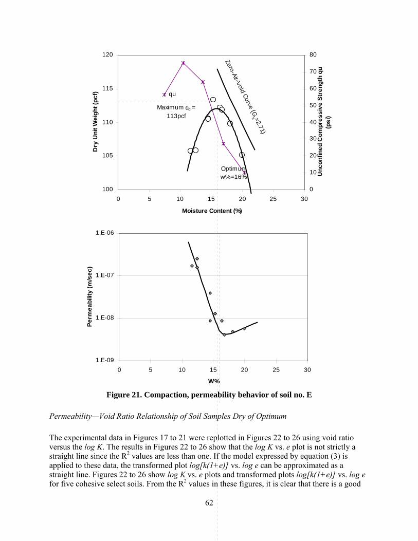
62
1.E-09
1.E-08
1.E-07
1.E-06
0 5 10 15 20 25 30
W%
Perm
eabi
lity
(m/s
ec)
Maximum 0d = 113pcf
Optimum w%=16%
Zero-Air-Void Curve (Gs =2.71)
qu
100
105
110
115
120
0 5 10 15 20 25 30
Moisture Content (%)
Dry
Uni
t Wei
ght (
pcf)
0
10
20
30
40
50
60
70
80
Unc
onfin
ed C
ompr
essi
ve S
tren
gth
qu(p
si)
Figure 21. Compaction, permeability behavior of soil no. E
Permeability—Void Ratio Relationship of Soil Samples Dry of Optimum
The experimental data in Figures 17 to 21 were replotted in Figures 22 to 26 using void ratio versus the log K. The results in Figures 22 to 26 show that the log K vs. e plot is not strictly a straight line since the R2 values are less than one. If the model expressed by equation (3) is applied to these data, the transformed plot log[k(1+e)] vs. log e can be approximated as a straight line. Figures 22 to 26 show log K vs. e plots and transformed plots log[k(1+e)] vs. log e for five cohesive select soils. From the R2 values in these figures, it is clear that there is a good

63
correlation between log[k(1+e)] and log e when the samples are compacted dry of optimum. However, the correlation on the wet side is very poor. The C and x values in the model
⎥⎦
⎤⎢⎣
⎡+
=e
eCkx
1 (equation [3]) can be obtained directly from these figures: x is the slope of the
straight line and C is the intercept. Table 10 summarizes these parameters.
From the data in Table 10, it can be seen that the exponent x ranges from about 11 to 22, which is similar to values determined for overconsolidated clay (Samarasinghe et al. 1982) and is much greater than that of normally consolidated clay, as presented by Sridharan and Nagaraj (2005). The exponent x on the wet side is much different than the values for normally consolidated clay, likely due to the low R2 values obtained.
Permeability—Compaction Variables Relationship
Using the empirical model suggested by Harrop-Williams (1985) as shown in equation (6), the ln k – x curves are plotted in Figures 27 to 32. The regression constants A and α were obtained from these figures and are shown in Table 11.
From Table 11, it can be seen that constant A ranges from -18.58 to -21.16 and α ranges from -4.97 to -7.1 with a relatively high correlation coefficient R2 (0.88 - 0.96), meaning 88% to 96% of the variance in permeability is explained by this model. The variation of these two constants is small because the five soils are all glacial till and their compaction methods are the same. By applying Harrop-Williams’s model to all the five soils, the regression constants for these Iowa cohesive select soils are obtained with A equal to -20 and α equal to -5.63. These constants are very similar to those suggested by Harrop-Williams (1985) (A = -19.873, α = -5.19) for compacted clay.
As suggested by Harrop-Williams (1985), A and α depend primarily on the soil type and level of compaction. In this study, the level of compaction is the same for all soils so that the soil type is the only factor that influences A and α. As discussed previously, the permeability of fine-grained soils is influenced by specific surface area, which can be correlated to some soil index properties, such as liquid limit, plasticity limit, plasticity index, and fine contents. These correlations were investigated, and it was found that strong correlations exist between constant A and P200*PI and α and LL. Figures 33 and 34 show the plots A versus P200*PI, and α versus LL, respectively. From Figures 33 and 34, it is clear that there is a good correlation of A with P200*PI (R2 = 0.95), and α with LL (R2 = 0.80).
These results indicate that a model using the liquid limit and the percent finer than the No. 200 sieve can estimate the permeability of these compacted clays.

64
y = 0.0062x14.755
R2 = 0.938
1.00E-09
1.00E-08
1.00E-07
1.00E-060 0.1 0.2 0.3 0.4 0.5 0.6
Void ratio e
Perm
eabi
lity
(m/s
ec)
y = 15.056x - 1.9432R2 = 0.9403
y = -2.0786x - 9.4268R2 = 0.1435
-9.5
-9
-8.5
-8
-7.5
-7
-6.5
-6
-5.5
-5-0.45 -0.4 -0.35 -0.3 -0.25 -0.2
loge
log[
k(1+
e)]
Dry sideWet side
Figure 22. Permeability versus void ratio relationship for Soil No. A

65
y = 0.1529x19.353
R2 = 0.9574
1.00E-08
1.00E-07
1.00E-060.44 0.46 0.48 0.5 0.52 0.54
e
Perm
eabi
lity
(m/s
ec)
y = 19.683x - 0.5398R2 = 0.9589
y = -7.52x - 10.006R2 = 0.5697
-8.5
-8
-7.5
-7
-6.5
-6
-5.5
-5-0.4 -0.35 -0.3 -0.25 -0.2 -0.15 -0.1
loge
log[
k(1+
e)]
Dry side
Wet Side
Figure 23. Permeability versus void ratio relationship for soil no. B

66
y = 0.2118x21.331
R2 = 0.9386
1.00E-09
1.00E-08
1.00E-07
1.00E-060 0.1 0.2 0.3 0.4 0.5 0.6
e
Perm
eabi
lity
(m/s
ec)
y = 21.663x - 0.3976R2 = 0.9404
y = 2.3861x - 7.1339R2 = 0.9453
-8.5
-8
-7.5
-7
-6.5
-6
-5.5
-5-0.4 -0.35 -0.3 -0.25 -0.2 -0.15 -0.1
loge
log[
k(1+
e)]
Dry side
Wet Side
Figure 24. Permeability versus void ratio relationship for soil no. C

67
y = 8E-05x10.242
R2 = 0.8341
1.00E-08
1.00E-07
1.00E-060 0.1 0.2 0.3 0.4 0.5 0.6 0.7
e
Perm
eabi
lity
(m/s
ec)
y = 10.582x - 3.7926R2 = 0.8429
y = 0.1973x - 7.7208R2 = 0.0264
-8
-7.5
-7
-6.5
-6
-5.5
-5-0.4 -0.35 -0.3 -0.25 -0.2
loge
log[
k(1+
e)]
Dry side
Wet side
Figure 25. Permeability versus void ratio relationship for soil no. D

68
y = 0.0004x15.562
R2 = 0.8739
1.00E-09
1.00E-08
1.00E-07
1.00E-060 0.1 0.2 0.3 0.4 0.5 0.6 0.7
e
Perm
eabi
lity
(m/s
ec)
y = 15.918x - 3.0642R2 = 0.8787
y = -0.0777x - 8.0834R2 = 0.0004
-8.5
-8
-7.5
-7
-6.5
-6
-5.5
-5-0.32 -0.3 -0.28 -0.26 -0.24 -0.22 -0.2
log e
log[
k(1+
e)]
Dry side
Wet side
Figure 26. Permeability versus void ratio relationship for soil no. E

69
Table 10. Permeability parameters for five cohesive select soils in Iowa
Soil No.
Optimum w%
Maximum dry unit weight
γd(pcf)
Dry side Wet side
x C (m/s) x C (m/s)
A 11.5 122 15.06 1.14E-02 -2.08 3.74E-10 B 14 116 19.68 0.29 -7.52 9.86E-11 C 13 118 21.66 4.00E-01 2.39 7.35E-08 D 11.6 122 10.58 1.61E-04 0.20 1.90E-08 E 16 113 15.92 8.63E-04 -0.08 8.25E-09
Table 11. Regression constants of five cohesive select soils from Iowa
Soil No.
optimum w %
Maximum dry unit weight γd
(pcf)
Variables
LL PL PI P200 (%) PI*P200A α R2
A 11.5 122 -21.16 -6.24 0.92 26 13 13 54.06 7.03 B 14 116 -18.58 -4.97 0.88 35 19 16 70.21 11.23 C 13 118 -19.42 -5.14 0.88 34 18 16 65.87 10.54
y = -6.2413x - 21.157R2 = 0.9222
-25
-20
-15
-10
-5
0-1.2 -1 -0.8 -0.6 -0.4 -0.2 0
x
lnK
Figure 27. Permeability versus compaction variables for soil no. A

70
y = -4.9731x - 18.582R2 = 0.8838
-25
-20
-15
-10
-5
0-1 -0.8 -0.6 -0.4 -0.2 0
x
lnK
Figure 28. Permeability versus compaction variables for soil no. B
y = -5.1403x - 19.42R2 = 0.8843
-25
-20
-15
-10
-5
0-1 -0.8 -0.6 -0.4 -0.2 0
x
lnK
Figure 29. Permeability versus compaction variables for soil no. C
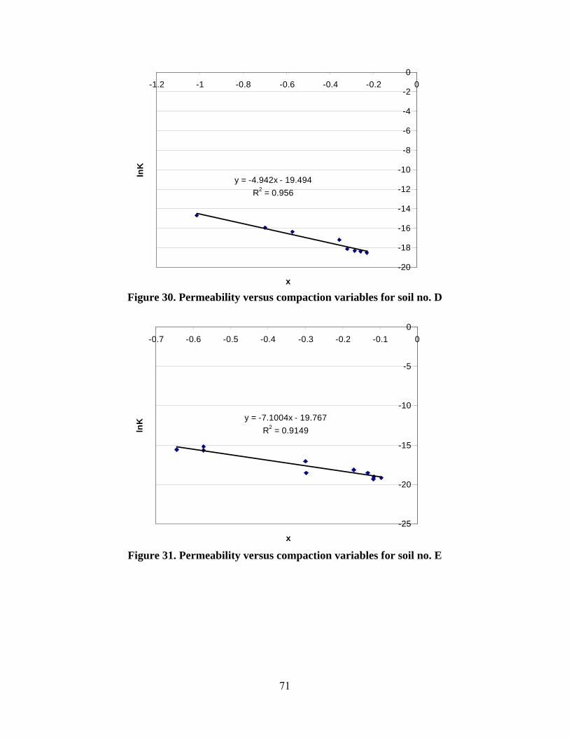
71
y = -4.942x - 19.494R2 = 0.956
-20
-18
-16
-14
-12
-10
-8
-6
-4
-2
0-1.2 -1 -0.8 -0.6 -0.4 -0.2 0
x
lnK
Figure 30. Permeability versus compaction variables for soil no. D
y = -7.1004x - 19.767R2 = 0.9149
-25
-20
-15
-10
-5
0-0.7 -0.6 -0.5 -0.4 -0.3 -0.2 -0.1 0
x
lnK
Figure 31. Permeability versus compaction variables for soil no. E

72
y = -5.6317x - 20.004R2 = 0.7214
-25
-20
-15
-10
-5
0-1.2 -1 -0.8 -0.6 -0.4 -0.2 0
x
lnK
Figure 32. Permeability versus compaction variables for all five soils
y = 0. 2393x2 - 3. 7782x - 6. 1767R2 = 0. 9472
- 21. 5
- 21. 0
- 20. 5
- 20. 0
- 19. 5
- 19. 0
- 18. 5
- 18. 00 2 4 6 8 10 12
PI * P200
A
Figure 33. A versus PI*P200 for all five Iowa cohesive select soils

73
y = 0. 1286x2 - 7. 6792x + 106. 55R2 = 0. 8045
- 9. 0
- 8. 0
- 7. 0
- 6. 0
- 5. 0
- 4. 0
- 3. 0
- 2. 0
- 1. 0
0. 00 10 20 30 40
LL
α
Figure 34. α versus LL for all five Iowa cohesive select soils
Comparison of Measured Permeability to NCHRP 1-37A Empirical Equations
As mentioned previously, equations (4) and (5) are incorporated in the EICM model to estimate the saturated permeability of compacted soil at optimum moisture content. The soil parameters used in these equations are P200, PI, and D60. To evaluate these equations, the ksat was calculated and compared to the measured values, as shown in Table 12 and Figure 35.
Table 12. Comparison of measured permeability to NCHRP 1-37A empirical equations
Soil No. D60 (mm) PI P200
calculated ksat (ft/hr) (from
eq. (3))
calculated kc (m/sec) (from
eq. (3)) Measured km (m/sec) kc/km
A 0.13 13 54 7.58E-06 6.42E-10 3.61E-09 0.18 B 0.06 16 70 3.33E-06 2.82E-10 3.33E-08 0.01 C 0.06 16 66 3.77E-06 3.19E-10 7.33E-09 0.04 D 0.1 10 54 1.05E-05 8.91E-10 1.31E-08 0.07 E 0.04 15 66 4.28E-06 3.63E-10 8.73E-09 0.04

74
1E- 10
1E- 09
1E- 08
1E- 07
1E- 06
1E- 05
1E- 04
1E- 03
1E- 02
1E- 01
1E+001 2 3 4 5
Perm
eabi
lity
k (
m/se
c)
Measur edPer meabi l i t y( m/ sec)Cal cul at edPer meabi l i t y( m/ sec)
Figure 35. Comparison of NCHRP 1-37A calculated permeability and measured
permeability
It can be seen from Figure 35 that the difference of measured and calculated permeability using equations (4) and (5) is between 1 to 2 orders of magnitude. One of the objectives of this study is to find an improved model to estimate permeability. A regression analysis from measured permeability and PI*P200 is given in Figure 36.
y = 0. 0946x2 - 1. 5209x + 1. 6472R2 = 0. 882
- 5. 0
- 4. 5
- 4. 0
- 3. 5
- 3. 0
- 2. 50 2 4 6 8 10 12
PI *P200
logK
(ft
/hr)
Figure 36. log K vs. PI*P200

75
Figure 36 shows that permeability of compacted soils can be expressed by PI*P200. Since PI*P200 is greater than one, the regression model is provided in a similar form to equation (5):
]65.1)(52.1)(095.0[ 2002
20010 +−= PIPPIPsatk (ft/hr). (10)
Although equation (10) has a similar form as equation (5), the permeability value obtained from each equation has one to two orders of magnitude difference, which indicates that ksat may as well depend on other factors.
According to Benson and Trast (1995), the initial saturation (Si) and compaction effort (E) are more important factors than P200 and PI. Therefore, Si and E were studied in this research. Equation (8) incorporated both factors and is applied. The comparison of calculated k from equation (8) and measured k is summarized in Table 13, which shows that if the initial degree of saturation is included in the model, the difference between calculated permeability and measured permeability is within one order of magnitude.
Overall, if PI, P200, LL, and compaction variables, such as γd and w%, are all incorporated in the model, according to equation (4) and Figures 33 and 34, permeability can be expressed as follows:
)ln(]6.106*68.7)(*13.0[2.6)*(78.3)*(24.0ln 2200
2200
dw
d
GwG
LLLLPPIPPIkγγ
γ−
+−+−−= . (11)
Equation (11) provides a general prediction model for permeability of compacted clay.
For Iowa cohesive select soils, A is about -20, α is about -5.63. This model can be simplified as follows:
)ln(63.520lndw
d
GwG
kγγ
γ−
−−= , (12)
where k = permeability of compacted soil (m/s), PI = plasticity index, P200 = percent finer than
No. 200 sieve, dγ = dry unit weight of compacted soil, wγ = unit weight of water, and G = specific gravity of soil.
To validate equations (11) and (12), all the test data is presented in Table 14.
It can be seen from Table 14 that the new model predicts the permeability very well; the ratio of predicted permeability and the measured permeability ranges from 0.16 to 1.78. Compared to equation (5), equation (11) is a more comprehensive model in that it incorporates the index properties (PI, P200, and LL), compaction characteristics, and initial degree of saturation (which is implied by moisture content, specific gravity, and dry unit weight). For Iowa soil, the permeability of select soil can be predicted by equation (12), even in the absence of the index properties.

Tab
le 1
3. C
ompa
riso
n of
mea
sure
d pe
rmea
bilit
y to
Ben
son
and
Tra
st’s
reg
ress
ion
mod
el (1
995)
Soil
No.
D
60
(mm
) PI
P 2
00
S i
calc
ulat
ed k
c (m
/sec
) (fr
om
eq. (
7))
Mea
sure
d k m
(m/s
ec)
k c/k
m
A
0.13
13
54
57
1.
39E-
9 3.
61E-
09
0.38
B
0.
06
16
70
20
6.5E
-8
3.33
E-08
1.
26
C
0.06
16
66
22
3.
23E-
8 7.
33E-
09
4.41
D
0.
1 10
54
35
1.
11E-
8 1.
31E-
08
0.85
E
0.04
15
66
45
4.
61E-
9 8.
73E-
09
0.53
T
able
14.
Val
idat
ion
of p
erm
eabi
lity
mod
el e
quat
ions
(9) a
nd (1
0)
Soil
No.
O
ptim
um
W%
Max
imum
dr
y
unit
wei
ght
γ d (p
cf)
G
LL
PLPI
P 2
00
(%)
PI*P
20
0
calc
ulat
ed
k c
(m/s
ec)
usin
g eq
(9)
calc
ulat
ed
k c
(m/s
ec)
usin
g eq
(10)
Mea
sure
d k m
(m
/sec
)
k c/k
m
eq(8
) k c
/km
eq
(9)
A
11.5
12
2 2.
7026
13
13
54
.1
7
2.37
E-09
6.
44E-
09
3.61
E-09
0.
66
1.78
B
14
116
2.69
35
19
16
70.2
11
.2
1.71
E-08
5.
35E-
09
3.33
E-08
0.
51
0.16
C
13
118
2.74
34
18
16
65.9
10
.5
1.01
E-08
7.
50E-
09
7.33
E-09
1.
38
1.02
D
11.6
12
2 2.
8425
15
10
54
.1
5.4
1.
11E-
08
1.22
E-08
1.
31E-
08
0.85
0.
93
E 16
11
3 2.
7133
18
15
66
.5
10
4.04
E-09
4.
37E-
09
8.73
E-09
0.
46
0.50
76

77
Conclusions
The permeability of five compacted cohesive select soils from Iowa were evaluated. Several conclusions were drawn from the results of this study.
1. Permeability test is reproducible, provided that the variance of test results is between 49% below the averaged value and 52% above the averaged value. The higher the moisture content, the higher the variance.
2. Air-dried samples have lower permeability than that of wet samples tested right after extruded from compaction mold. The permeability of air-dried samples is from about 56% to 95% of that of wet samples. Air-drying has less effect on the results when the samples are compacted dry of optimum than when they are compacted wet of optimum.
3. Permeability of compacted soil decreases with moisture content when it is dry, while the permeability increases slightly with moisture content when the soil gets wetter. The lowest permeability occurs at a moisture content of about 2% to 4% wet of optimum.
4. There is a good correlation between log[k(1+e)] and log e when the samples are compacted dry of optimum. However, the correlation in the wet side is very poor. When equation (3) applies, the x value ranges from 11 to 22 for overconsolidated clays.
5. Permeability can be predicted using Harrop-Williams (1985) model (equation [6]), where A ranges from -18.58 to -21.16 and α ranges from -4.97 to -7.1 for Iowa cohesive soils.
6. The difference between the measured permeability and the calculated permeability using EICM model is one to two orders of magnitude.
7. Equations (11) and (12) provide a more comprehensive model based on the Harrop-Williams (1985) model to predict compacted soil permeability, which incorporated PI, LL, P200, w%, and γdry.

78
FIELD INVESTIGATION OF SETTLEMENT ADJACENT TO HIGHWAY CULVERTS
Introduction
Culverts are commonly installed to deal with the highway drainage needs. Installation of a culvert generally necessitates an excavation in natural or fill materials, with subsequent compaction of soil materials to fill back in the excavated materials. Unfortunately, settlement adjacent to highway culverts has often been found shortly after the road is open to traffic. Although not perceptible to the naked eye, the settlement near a culvert is noticeable in a vehicle driving though these locations. To address this issue, an investigation of the causes of the problem and the development of a solution was undertaken.
Settlement is a common problem following culvert installation and is often due to poorly compacted sand and rock backfill (crushed lime stone) materials. Displacement of soft material or piping along the culvert can cause significant damage to the culvert. Poorly compacted backfilled soils are subject to substantial volume reduction once saturated (Selig 1990). This phenomenon is called collapse compression. Collapse occurs because the backfill soils lose capillary tension when they become saturated, causing the soil particles to settle into a denser packing. Selig (1990) noted that collapse compression strain decreases as the degree of compaction increases and diminished to an insignificant amount once the compaction reaches 85% to 90% of standard Proctor unit weight. The settlement of backfill materials causes bumps on the pavement surface and distress to the drain pipes buried in the sand backfill. This distress might lead to cracking of pipes, resulting in leakage of water into the subsoil. If the subsoil consists of problematic soils, such as expansive or collapsible loess soils, seeping of water into these soils could trigger further intricate problems of volume changes that are detrimental to the engineering performance of pavements. Although there is considerable information available on the design and construction of new culverts, there is little information in the literature on how to repair culvert problems and even less on how to rehabilitate, strengthen, or retrofit upgrade culverts. Initiating any kind of remedial measures requires a thorough investigation of the soil profile and properties of different soils in different strata.
Figure 37 shows the general nature of the problem. The two-foot diameter pipe under the poorly compacted rockfill is subjected to distress owing to the settlement of the rockfill under traffic loads. The effect of soil settlement is shown in Figure 38. Field investigation indicates that settlement occurs near the pavement surface right above the pipe. Settlement of backfill material and movement of the structure can have serious structural consequences in pipes, such as misalignment or rupture of the pipe system. A stable soil envelope around pipes is necessary for side support that will reduce settlement of rigid pipe. Figure 39 shows the remediation alternatives. It is proposed that, to ward off large amounts of settlement, the backfill above the center of pipe is replaced by flowable mortar, the major components of which are fly ash, cement, sand, and water.
The objectives of this portion of the study were to (1) investigate culvert settlement problems in Iowa, (2) review the remediation methods in the literature, and (3) study the select and flowable mortar as backfill options.

79
Paver
Gr ader
2% 2%
2%2%
PCC
Rock10.5-13.5''
6''
Select (Good sand, glacial till)
0-3'' (Shallow)>3'' (Deep)
Pi pe Figure 37. Cross-section of pavement
(a) Rigid pipe (b) Flexible pipe
Figure 38. The effect of soil settlement on (a) rigid and (b) flexible pipes (US Army 1959)
Sand or rock
Flowable mortar
(a) Shallow Pipe
Pipe
300 lbs Fly ash100 lbs Cement2700 lbs Sand70 gals of water
Sand or rock without mortar
(b) Deep Pipe
Pipe
Figure 39. Proposed treatment of materials surrounding the pipe (Iowa DOT specification
2001)
Background
The pipe (culvert) and the soil surrounding it work as an integral system, which means that weakness in the surrounding soil affects the performance of the drainage pipe. Thus, the quality of backfill materials is of vital importance to the pipeline safety regarding bearing capacity and settlement issues. For culvert systems, compacted, well-graded, angular, granular backfill materials provide the best structural support. These backfill materials comprise primarily selected soils restricted to A-1, A-2, and A-3 classifications and are compacted to a density of more than 90% of standard Proctor maximum dry unit weight (US Army 1959). However, the

80
use of conventional backfill materials is hard to meet the compaction criteria due to site restriction, soil conditions, equipment limitation, and workmanship, especially in the area right next to the pipe and below the spring line. Therefore, materials that can be compacted easily or possess a high stability to resist the deformation from the repeated loading have recently been used. These materials are granular backfill, concrete sand, well-graded crushed stone, recycled portland cement concrete, flowable mortar, etc.
The following factors are considered when selecting a backfill material: ease of compaction, labor requirements, degree of inspection, and cost (US Army 1959). Granular backfill or sand and flowable mortar would be the best choices. Currently, flowable mortar is becoming more and more popularly used as pipeline backfill (ACI Report 229R-94 1994). As the American Concrete Institute (ACI) Report 229R-94 (1994) outlines, this material possesses some potential advantages over conventional soil fill. A literature review of this material is provided in the following section.
Controlled Low-Strength Material
Flowable mortar is also called “Controlled Low Strength Material-Controlled Density Fill” (CLSM-CDF) by ACI Committee 229 (ACI Report 229R-94 1994). It is a low-strength material mixed to a wet, flowable slurry and used as an economical fill or backfill material. In the case of CLSM-CDF, the material components, when mixed and placed, must possess the following properties: flowability, removability, strength, and a competitive price. (ACI Report 229R-94 1994) The basic components for CLSM-CDF are portland cement, fine aggregate, fly ash, and water.
Portland Cement
Type I or Type II portland cement that conforms to ASTM C 150 (ASTM 1995) is usually used. The amount is approximately 3% of the total mixture’s weight. The purpose of the cement is to provide cohesion and strength control in the mixtures. For typical backfills where future removability is anticipated, the compressive strength (c’) should be less than 100 psi at 28 days (ACI Report 229R-94 1994).
Fine Aggregate
The fine aggregate, known as filler, makes up the major portion (72%) of a typical CLSM-CDF mixture. This material was utilized because of its availability and it proved to be an excellent CLSM-CDF filler. The filler should possess adequate gradation similar to the requirement as set forth in ASTM C 33 (ASTM 1995) to insure proper flowability. Another filler material consideration is the material’s particle angularity. Naturally, a material containing particles with sharp edges will result in less desirable flow characteristics. Aggregates, such as pea gravel with sand, sand with 10% silt, and quarry waste products, have been proved to be working well in CLSM.

81
Fly Ash
Fly ash used in portland cement concrete usually complies with ASTM C 618 (ASTM 1995). Fly ash makes up approximately 8% of a typical CLSM-CDF mixture (ACI Report 229R-94 1994). The majority of the CLSM research has been conducted using Class F fly ash (ACI Report 229R-94 1994). In addition to finding a suitable use for an industrial by-product, fly ash used in CLSM mixtures also provides several benefits, such as better workability, lower cost, reduced hydration heat, reduced shrinkage upon drying, and greater strength gain beyond the first 28 days (Sargand et al. 2001).
Water
Water is used in a CLSM mixture for flowability and hydration. Water increases in CLSM mixtures do not affect its compressive strength. However, water reductions below the design level will increase the compressive strength. A typical CLSM-CDF mixture would consist of approximately 17% water.
Flowable Fill Design
The purpose of flowable fill is to provide a structural substitute for compacted granular soil. As such, it needs sufficiently low strength to allow for future excavation while providing adequate support for the pipe (Hitch et al. 2002). Discussions with producers of flowable fill and literature research yielded the flowable fill specifications shown in Table 15. The recommended starting point for lab investigations for CLSM mix design for strengths of 100 psi or less is shown in Table 16.
Flowability
CLSM is able to flow into places that are hard to reach (haunches) or in narrow trenches where space limited, thus eliminating all labor requirements for placement. Flowability tests were conducted on all trial batches by placing a freshly mixed sample of CLSM in a 75 mm diameter (3 in.) by 150 mm (6 in.) high open-ended tube and quickly lifting the tube vertically, allowing the CLSM sample to slump into a circular mound. The circular sample spread was then measured. A minimum acceptable spread of 200 mm (8 in.) and no segregation of water were adopted acceptance criteria based on guide specifications of the Texas Aggregates and Concrete Association. To achieve this number, a water/solid ratio of 0.4 to 0.6 can be used for flowability design.
Table 15. Flowable fill specifications (Hegarty et al. 1998)
Property Value Unit weight 142 pcf (2275 kg/m3) Slump (max) 9 in. (22.8 cm)
Water/cement ratio 0.68 28-Day compressive strength (max) 100 psi (70310 kg/m2)

82
Table 16. Flowable fill mix design
Property Value Portland cement (Type I) ASTM C150 100 lbs/yd3 (59.32 kg/m3)
Fly ash, ASTM C618 Class F 300 lbs/yd3 (177.96 kg/m3) Aggregate, ASTM C33 2600 lbs/yd3 (1542.32 kg/m3)
Water 584 lbs/yd3 (346.43 kg/m3) Unit weight 127.8 pcf (2050 kg/m3)
Compressive strength: 14 days 60 psi (0.41 MPa) Compressive strength: 28 days 60 psi (0.41 MPa) Compressive strength: 90 days 160 psi(1.10 MPa)
California Bearing Ratio (CBR), %: 0.1 in. 19.7 California Bearing Ratio (CBR), %: 0.2 in. 23.7 Removability
If the CLSM is to be excavated in the future, removability must be considered. As stated in ASTM D 4832 (ASTM 1995), the only structural requirement for the flowable mortar is that its minimum compressive strength is slightly higher than the surrounding soil; 50 psi is a typical value. However, to ensure removability, unconfined compressive strength of less than 100 psi is required.
Advantages of CLSM Compared to Conventional Backfills
First, CLSM does not form void spaces during placement like soils and will not settle under loads. CLSM’s load-carrying capacity is higher than compacted soils, and its relatively low long-term strength (50 to 100 psi) makes it easy to remove in the future. Second, using CLSM is cost-effective because its placement procedure is less labor intensive. Brewer et al. (1991) made an illustrative comparison based on the material prices in Ohio and found that for a roadway trench with the dimensions of 3 ft wide, 6 ft deep, and 40 ft long, the total cost of the CLSM and conventional backfill is about equal. However, every one-foot reduction in trench width in this example represents a backfill cost reduction of $255.64 when using CLSM (Brewer et al. 1991). The trench width is reduced because conventional compaction requires additional access width around the culvert, and CLSM does not require significant testing and inspection during placement, both of which reduce labor cost.
The end use of the CLSM mixture must be known to design the proper mixture. For example, if removability is not to be a factor, then the compressive strength 100 psi or more would not be a factor. Similarly, if the mixture was to be pumped, then flowability could be reduced.
Flowable Mortar in Iowa
Iowa DOT specifications for highway and bridge construction have specified that flowable mortar can be used as backfill material around culvert pipes. The materials, including cement, fly ash, fine aggregate, and admixtures, must meet the following requirements: cement should be type I (ASTM C 150), fly ash should be either Class F or Class C (AASHTO M295), and fine

83
aggregate should be natural sand with the gradation of 100% passing ¾ inch and 0%-10% passing No. 200 sieve.
Flowable mortar is being used by the Iowa DOT for culvert backfill with the following requirements: granular backfill for half the height of the culvert and flowable mortar for a maximum of five feet above the culvert. The granular backfill ensures that the culvert does not float and acts as a filter to keep from plugging the drainage system. The required subgrade treatment must be between the pavement and the flowable mortar.
Forensic Investigation
The pavement surface of Highway 18 (mile post 195), Highway 218 (mile post 211), and Highway 330 (mile post 12) were investigated in this research (see Figure 40). The locations of these sites are listed in Table 17. When driving through these sites, bumps could be felt on the pavement surface above the pipe. Due to limited time, a pavement surface topographic profile was taken only for Highway 18 and was plotted in Figure 41. The investigation revealed bumps across the lanes on the pavement surface. The “bump” shown in Figure 41 is about 0.2 in. deep and it is 20 to 30 ft away from the pipe. Figure 42 shows the pipe location and the pavement surface. Highway 330S was selected for a detailed investigation because it had maximum settlement of 0.5 in. Soil samples were collected for laboratory testing. One-dimensional consolidation tests and consolidated undrained triaxial tests (CU) were performed. For comparison, flowable mortar strength was obtained from Mr. John Vu from the Iowa DOT (Vu, personal communication 2005).
Figure 40. Locations of three investigated sites

84
Table 17. Locations of investigated sites
No. Highway Mile post County 1 HW18E 195.65 Cerro Gordo (near Mason City) 2 HW18E 195.73 Cerro Gordo (near Mason City) 3 HW18E Cerro Gordo (near Mason City) 4 HW18E Cerro Gordo (near Mason City) 5 HW18E Cerro Gordo (near Mason City) 6 HW218N 211.65 Bremer (Waverly City) 7 HW330S 12.15 Marshall 8 HW330S 12.4 Marshall 9 HW330S 12.9 Marshall 10 HW330S 13.05 Marshall 11 HW330S 13.3 Marshall
8.5
8.55
8.6
8.65
8.7
8.75
0 10 20 30 40 50 60distance from Point#4 (ft)
Elev
atio
n fro
m th
e bo
ttom
of c
uver
t (in
.) Elevation (ft) (before)
Elevation (ft) (after)
Figure 41. Topographic profile at mile post 195, Highway 18, Iowa

85
Figure 42. Pavement surface distortion, Highway 18 east (mile post 195), Iowa
Laboratory Testing
Soil parameters that are usually considered in the design of pipe are soil type, soil density, moisture content, modulus of elasticity, coefficient of lateral earth pressure, friction angle, etc. Shelby tube samples were collected from three bore holes of the embankment at Highway 330, mile post 13.30. Borehole 1 is 2.5 meters south of the culvert; samples were collected up to a depth of 13 ft (4 m). Borehole 2 is right above the culvert; samples were collected up to a depth of 7 ft (2.2 m), which is the top of pipe. Borehole 3 is 5 meters north of the culvert and drilled down to 15.4 ft (4.7 m). The boring logs are provided in Table 18; the boring location is schematically shown in Figure 43.
Moisture Content, Compaction, and UCS
It can be seen from Figure 44 that the moisture content is consistent at about 20%-25% of BH1 and BH3, while it is much dryer at BH2 at the range of 13%-18%.
The moisture content at compaction greatly affects the compaction density and unconfined compressive strength of select soils. A 2% moisture content difference can lead to about 50 kg/m3 compaction density change. The select materials have an averaged unconfined compressive strength of about 400 kPa at optimum moisture content. The difference in strength over 2% moisture content is quite significant (more than 100 kPa). The information confirms the importance of moisture content during compaction. According to the specifications 2102.04 (Iowa DOT Specification 2001), the moisture content limits for select soil is from 2.5% dry of optimum to no upper limit during compaction. Since there is no upper limit during compaction, it is sometimes believed that the contractor may compact the select when it is too wet, which is
Drainage pipe

86
hard to compact adequately and will result in the low strength of backfill. The stability decreases very quickly once the moisture content exceeds the optimum. The soil is so unstable that it should be obvious that the roller would not walk-out. Because there currently is no upper limit on moisture content for the select soils, the specifications should be changed to ensure proper moisture content during compaction Also, this change would help field staff enforce the discing and drying before compaction. This is essential to obtain good density and stability.
Consolidated-Undrained Triaxial Tests (CU)
For comparison purposes, CU tests were conducted in general accordance to ASTM D 4767-95 “Standard Test Method for Consolidated-Undrained Triaxial Compression Test for Cohesive Soils” (ASTM 1995). Three samples were tested for each bore hole at different confining pressures (25, 45, and 65 kPa for BH1; 15, 30, and 45 kPa for BH2) to access the shear strengths of the soils. The confining pressures are equal to the effective overburden pressure in the field. The specimen was initially fully consolidated to an isotropic confining pressure. A loading rate of 0.05 in. (approximately 1% axial strain) per minute was used in performing the tests. This led to testing times of approximately 20 minutes because the tests were continued to 20% axial strain. Peak deviator stress was used as the failure criterion if the peak was reached at 10% axial strain or less. If the peak did not occur below 10% axial strain, the deviator stress at 10% axial strain was used as the failure criterion. Figures 45 and 46 show the stress-strain and pore water pressure characteristics. During the compression, the pore pressure increased and then decreased to below the original value. It shows that the soils are overconsolidated—contracted (pore pressure increased) at the beginning of compression and then dilated (pore pressure decreased).The strength ranges from 115 to 221 kPa, which is much lower than the averaged unconfined compressive strength (400 kPa) at optimum moisture contents. It is believed that the soil around the pipe was not compacted at optimum moisture content. The stress path of these two bore holes materials is shown in Figures 47 and 48. It is evident from Figures 47 and 48 that, at the confining pressures at which the soils were tested, the soils exhibited both cohesion and friction angle. Confining pressure (σ3), peak deviator stress ([σ1-σ3]f), cohesion (c), and friction angles (φ) are summarized in Table 19.

Tab
le 1
8(a)
. Bor
ing
logs
of H
ighw
ay 3
30S—
bore
hole
1
Bor
ing
Log
Proj
ect:
O
ptim
izat
ion
and
Man
agem
ent o
f Ear
thw
ork
Mat
eria
ls (C
ulve
rt, a
t H
W33
0S, M
P 13
.30.
2.5
m so
uth
of th
e cu
lver
t) B
orin
g N
o.:
1
Rep
ort
Dat
e:
6/12
/200
6 St
art:
10
:00a
m, 6
/12/
2006
Loc
atio
n:
Fairf
ield
, Jef
fers
on, I
A
Fini
sh:
3:00
pm, 6
/12/
2006
Log
ged
By:
Lo
ngjie
Hon
g E
quip
men
t T
ype:
D
rill R
ig
Dri
lling
C
rew
: Sc
haef
er, B
rian,
Lon
gjie
Sa
mpl
ing
Met
hods
: 1.
She
lby
Tube
-2.8
inch
dia
met
er, 2
.5ft
segm
ent
Dep
th b
elow
su
rfac
e (in
) G
raph
ical
Log
Sh
elby
Tub
e#
Top
Dep
th,
(in)
Leng
th, (
in)
Bot
tom
D
epth
, (in
) M
ater
ial D
escr
iptio
n γt
(kN
/m3 )
σv (k
Pa)
σ3 (k
Pa)
Moi
stur
e C
onte
nt
(%)
33
To
p B
otto
m
64
1
33
31
64
2 tri
axia
l sam
ples
, 1
cons
olid
atio
n sa
mpl
e 20
.85
17.5
33
.9
25.0
20
.8
86
2
63
23
86
2 tri
axia
l sam
ples
, 1
cons
olid
atio
n sa
mpl
e 18
.37
29.4
40
.1
35.0
21
.9
116
3
86
30
116
3 tri
axia
l sam
ples
, 1
cons
olid
atio
n sa
mpl
e 19
.05
41.6
56
.1
45.0
22
.4
144
4
116
28
144
3 tri
axia
l sam
ples
, 19
56
.0
69.5
55
.0
22.4
158
5
114
44
158
2 tri
axia
l sam
ples
, 1
cons
olid
atio
n sa
mpl
e 19
.57
56.7
78
.5
65.0
22
87

Tab
le 1
8(b)
. Bor
ing
logs
of H
ighw
ay 3
30S—
bore
hole
2
Bor
ing
Log
Proj
ect:
O
ptim
izat
ion
and
Man
agem
ent o
f Ear
thw
ork
Mat
eria
ls (C
ulve
rt, a
t H
W33
0S, M
P 13
.30.
abo
ve th
e cu
lver
t) B
orin
g N
o.:
2
Rep
ort
Dat
e:
6/12
/200
6 St
art:
10
:00a
m, 6
/12/
2006
Loc
atio
n:
Fairf
ield
, Jef
fers
on, I
A
Fini
sh:
3:00
pm, 6
/12/
2006
Log
ged
By:
Lo
ngjie
Hon
g E
quip
men
t T
ype:
D
rill R
ig
Dri
lling
C
rew
: Sc
haef
er, B
rian,
Lon
gjie
Sa
mpl
ing
Met
hods
: 1.
She
lby
Tube
-2.8
inch
dia
met
er, 2
.5ft
segm
ent
Dep
th b
elow
su
rfac
e (in
) G
raph
ical
Log
Sh
elby
Tub
e#
Top
Dep
th,
(in)
Leng
th, (
in)
Bot
tom
D
epth
, (in
) M
ater
ial D
escr
iptio
n γt
(kN
/m3 )
σv (k
Pa)
σ3 (k
Pa)
Moi
stur
e C
onte
nt
(%)
24
To
p B
otto
m
31
1
24
7 31
1
cons
olid
atio
n sa
mpl
e 20
.93
12.8
16
.5
15.0
14
64
2
31
33
64
2 tri
axia
l sam
ples
, 1
cons
olid
atio
n sa
mpl
e 20
15
.7
32.5
25
.0
17.2
85
3
64
21
85
3 tri
axia
l sam
ples
, 1
cons
olid
atio
n sa
mpl
e 19
.96
32.4
43
.1
35.0
19
.2
88

Tab
le 1
8(c)
. Bor
ing
logs
of H
ighw
ay 3
30S—
bore
hole
3
Bor
ing
Log
Proj
ect:
O
ptim
izat
ion
and
Man
agem
ent o
f Ear
thw
ork
Mat
eria
ls (C
ulve
rt, a
t H
W33
0S, M
P 13
.30.
5m
nor
th o
f the
cul
vert
175
inch
es so
uth
of
stat
ion
1861
) B
orin
g N
o.:
3
Rep
ort
Dat
e:
6/12
/200
6 St
art:
10
:00a
m, 6
/12/
2006
Loc
atio
n:
Fairf
ield
, Jef
fers
on, I
A
Fini
sh:
3:00
pm, 6
/12/
2006
Log
ged
By:
Lo
ngjie
Hon
g E
quip
men
t T
ype:
D
rill R
ig
Dri
lling
C
rew
: Sc
haef
er, B
rian,
Lon
gjie
Sa
mpl
ing
Met
hods
: 1.
She
lby
Tube
-2.8
inch
dia
met
er, 2
.5ft
segm
ent
Dep
th b
elow
su
rfac
e (in
) G
raph
ical
Log
Sh
elby
Tub
e#
Top
Dep
th,
(in)
Leng
th, (
in)
Bot
tom
D
epth
, (in
) M
ater
ial D
escr
iptio
n γt
(kN
/m3 )
σv (k
Pa)
σ3 (k
Pa)
Moi
stur
e C
onte
nt
(%)
24
To
p B
otto
m
46
1
24
22
46
2 tri
axia
l sam
ples
, 2
cons
olid
atio
n sa
mpl
e 20
12
.2
23.4
20
.0
23
56
2
40
16
56
2 tri
axia
l sam
ples
, 1
cons
olid
atio
n sa
mpl
e 20
.3
20.6
28
.9
25.0
22
.5
78
3
64
14
78
2 tri
axia
l sam
ples
, 20
32
.5
39.6
35
.0
23.3
114
4
94
20
114
3 tri
axia
l sam
ples
, 1
cons
olid
atio
n sa
mpl
e 19
.58
46.7
56
.7
50.0
22
.2
146
5
120
26
146
4 tri
axia
l sam
ples
, 1
cons
olid
atio
n sa
mpl
e 19
.53
59.5
72
.4
65.0
23
.2
185
6
160
25
185
4 tri
axia
l sam
ples
, 1
cons
olid
atio
n sa
mpl
e 19
.66
79.9
92
.4
80
21.9
89

90
BH3
BH2
BH1
North
South
Traffic
Pipe
gravel shoulder
5m
2.5m
Figure 43. Schematic boring locations on Highway 330S
HW330, MP13. 30
0
50
100
150
200
0 5 10 15 20 25w%
Dept
h (i
n.)
BH1BH2BH3
Figure 44. Moisture content profile of the embankment

91
σ'3=25kPa
σ'3=65kPa
σ'3=45kPa
0
50
100
150
200
250
0 5 10 15 20 25
ε(%)
σ 1- σ
3(kPa
)
σ'3=45kPa
σ'3=65kPa
σ'3=25kPa
-100
-80
-60
-40
-20
0
20
40
60
0 5 10 15 20 25
ε(%)
u(kP
a)
Figure 45. Stress-strain curves and pore pressure curve for BH1

92
σ'3=30kPa
σ'3=45kPa
σ'3=15kPa
0
20
40
60
80
100
120
140
160
0 5 10 15 20 25
ε(%)
σ 1- σ
3(kPa
)
σ'3=30kPa
σ'3=15kPa
σ'3=45kPa
-40
-30
-20
-10
0
10
20
30
40
0 5 10 15 20 25
ε(%)
u(kP
a)
Figure 46. Stress-strain curves and pore pressure curve for BH2

93
c=12.9 kPaφ = 34.70
45 kPa
65 kPa
25 kPa
y = 0.5691x + 10.611R2 = 1
0
10
20
30
40
50
60
70
80
90
100
110
120
-20 0 20 40 60 80 100 120 140 160 180 200 220
p, p' (kPa)
q (k
Pa)
TSP
ESP
Figure 47. Stress path for BH1
30 kPa15 kPa
45 kPa
y = 0.3375x + 34.501R2 = 0.9888
c = 37kPa, φ =200
0
10
20
30
40
50
60
70
80
90
0 20 40 60 80 100 120 140 160p, p' (kPa)
q (k
Pa)
TSP
ESP
Figure 48. Stress path for BH2

94
Table 19. CU triaxial tests summary
Bore Hole σ3 (kPa) (σ1-σ3)f (kPa) c (kPa) φ (0)
BH1 25 115
13 35 45 168 65 221
BH2 15 123
37 20 30 132 45 151
Consolidation Tests
Consolidation tests were conducted according to ASTM D 2435-96 “Standard Test Method for One-Dimensional Consolidation Properties of Soils” (ASTM 1995). The purpose of these tests was to obtain the parameters for settlement analysis. The results are presented in Table 20. From Table 20, it is noted that the soils are normally consolidated or slightly overconsolidated, with an OCR of 1 to 8. The coefficient of consolidation, Cv, ranges from 2 to 13 (x10-3 cm2/sec).
Table 20. Summary of consolidation tests
Boring No.
Shelby Tube
Sample No.
Depth (m)
pc' (kPa)
Compression Index Cc
γt (kN/m3) overburden pressure p'
(kPa)
Coefficient of Consolidation Cv (x10-3 cm2/sec)
OCR
BH1
ST1 1.23 85 0.14 21 26 3.4 3 ST2 1.89 60 0.173 18 35 12.9 2 ST3 2.57 78 0.103 19 49 2.9 2 ST5 3.45 75 0.127 20 68 3.3 1
BH2 ST1 0.7 110 0.139 21 15 8.3 8
BH3 ST2 1.22 110 0.136 20 25 2.9 4 ST5 3.38 70 0.147 20 66 2.5 1 ST6 4.38 88 0.196 20 86 4.7 1
Flowable Mortar Tests
Article 2506.02 (Iowa DOT specification 2001) allows up to 70 gallons of water per cubic yard of flowable mortar. The amount of water in the mix will be an important factor for fluidity and strength of the mix. In order to obtain the compressive strength that would be close to that of the cohesive select soil, a few mix designs were evaluated by John Vu (Pipe backfill report 2005). Samples were cast in the plastic molds with holes at the bottom, and then the molds were set on a layer of granular backfill to determine the compressive strength. The strength for three different mixes is summarized in Table 21.

95
Table 21. Summary of the flowable mortar strength of different mixes
Age, days Mix Design 1 Mix Design 2 Mix Design 3 67 gal. (psi) 45 gal. (psi) 55 gal. (psi)
5 101 140 161 7 107 174 252 14 158 333 388 28 259 723 613
Mix Design 1
This mix design meets Iowa DOT requirement for both critical and noncritical applications with a time of efflux of 11 seconds when 67 gallons of water per cubic yard was used to backfill the pipe from the spring-line to the top of the pipe. There was no problem with the efflux time for this mix. It flowed very well. Figure 49 shows the construction of pipe using flowable mortar as backfill.
Figure 50 shows that the flowable mortar was strong enough after 24 hours to support the inspector’s weight. The stability reading measured with the Clegg Hammer showed that the strength was equal to a layer of six inches of crushed stone.
Figure 49. Pouring the flowable mortar
Mix Design 2
This flowable mix design did not flow. The efflux time was not tested, but it was very obvious that it would not flow through the testing cone. It was also noted that the strength was too high. For an open trench application, fluidity is not a problem. However, the strength is now a concern.

96
Figure 50. Strength after 24 hours
Mix Design 3
In order to determine what the minimum amount of water in the mix should be, another flowable mortar mix with 55 gallons was used. This mix, when tested for the efflux, did not flow at all. As before, flowable mortar cylinders were cast for compressive strength.
The compressive strength for this mix was still too high when compared with the UCS data for the cohesive select soil. The recommendation for the flowable mix design is the current design in the Iowa DOT specifications. There are two main reasons for this recommendation. The first reason is the lower strength, and the second reason is the fluidity and the ability to penetrate into the granular backfill layer. It will solve the “dip” problem and not create a “bump” problem.
Cost
The average cost per location as designed is about $2,100. However, depending on the contractor’s operation, the cost may be higher. For example, when the contractor placed the pipe in the cut situation, the contractor cut the trench wide enough to use the pipe bedding machine. If the contractor gets paid for only the plan quantity for granular backfill (GB) and flowable mortar (FM), the contractor may use some of the material that was excavated to backfill the trench. This may lead to a settlement problem.
Numerical Analysis of Pavement Settlement
Settlement analysis was performed using Sigma/W provided by Geo-Slope. (Geo-Slope 2007) The purpose of this analysis was to analyze the amount and shape of settlement on pavement surfaces using different backfill materials, including conventional backfill soils, sand and gravel, and flowable mortar. Comparisons were made based on the analysis.

97
Input parameters are listed in Table 22. The elastic modulus of soil was obtained by taking the slope of stress strain curves in Figures 47 and 48. The averaged value was about 10 MPa, which was in the range of soft clay, as shown in Table 23. The elastic modulus of gravel (96 MPa) was taken directly from Table 23. The elastic modulus of flowable mortar was obtained from equation (13) (ACI 318-07 2007).
'5.1 043.0 ccc fwE = , (13)
where Ec = modulus of elasticity (MPa), wc = unit weight of flowable mortar (kg/m3), and fc’ = compressive strength of flowable mortar (MPa).
Table 22. Summary of the materials properties in Sigma/W analysis
Materials Elastic modulus E (MPa) unit weight γ (kN/m3) Soil 10 20
Flowable mortar 8400 21 Gravel 100 21
Table 23. Typical elastic moduli of soil (EM 1110-1-1904 1990)
Soil Es, MPa (tsf)
Clay
Very soft clay 0.48-4.8 (5-50) Soft clay 4.8-19.2 (50-200)
Medium clay 19.2-48 (200-500) Stiff clay, silty clay 48-96 (500-1000)
Sandy clay 24-192 (250-2000) Clay shale 96-192 (1000-2000)
Sand
Loose sand 9.6-24 (100-250) Dense sand 24-96 (250-1000)
Dense sand and gravel 96-192 (1000-2000) Silty sand 24-192 (250-2000)
Based on the tested compressive strength of flowable mortar shown in Table 21, which is 613 psi (4.23 MPa) from flowable mortar mix design 3, and the unit weight of flowable mortar of 130 pcf (2085 kg/m3), the Ec is 8,420 MPa.
From the field investigation, the pipe was buried 7 feet (2.1 m) deep from the surface and was 2 feet (0.6 m) in diameter. The model was set in Sigma/W for three different materials: soil, gravel, and flowable mortar. Based on the Iowa DOT specifications, granular backfill was placed to half the height of the culvert and flowable mortar was set to a maximum of 5 feet (1.5 m) above the culvert.
The trench width was about 6.6 ft (2 m). A soil matrix of 4 m wide was also analyzed in order to see the “dip” problem. From the parametric study, the width of the trench has no effect on the settlement result (see Figure 51[a] and [b]).

98
The edges of the trench were assumed to be fixed in the x direction and free in the y direction. From 4 m deep below the pavement surface, soils were assumed to be fixed in both directions. Analysis results are shown in Figure 51.
It is noted from Figure 51 that the surface settlement is about 1.4 in. (0.035 m) for soil backfill, while it is only about half (0.018 m) for flowable mortar or gravel backfill (0.02 m). The settlement contour also shows that there is a “bump” on the pavement surface for soil backfill, but that the “bump” does not exist for flowable mortar or gravel backfill.
2 feet (0.6 m)
7 feet (2.1 m)
settlement contour
1.4 inches (0.035 m)
Soil
Soil
Metres0.5 1.0 1.5 2.0 2.5 3.0 3.5
-0.5
0.0
0.5
1.0
1.5
2.0
2.5
3.0
3.5
4.0
Figure 51(a). Settlement contour of pipe buried in soil (2 m wide trench)

99
2 feet (0.6 m)
7 feet (2.1 m)
settlement contour
Soi l
1.4 inches (0.035 m)
Metres-0.5 0.0 0.5 1.0 1.5 2.0 2.5 3.0 3.5 4.0
-0.5
0.0
0.5
1.0
1.5
2.0
2.5
3.0
3.5
4.0
Figure 51(b). Settlement contour of pipe buried in soil (4 m wide trench)

100
2 feet (0.6 m)
7 feet (2.1 m)
settlement contour
Gravel
Soil
Soil
Flowable mortar
0.7 in (0.018m)
Metres0.5 1.0 1.5 2.0 2.5 3.0 3.5
-0.5
0.0
0.5
1.0
1.5
2.0
2.5
3.0
3.5
4.0
Figure 51(c). Settlement contour of pipe buried in gravel and flowable mortar (2 m wide
trench)

101
2 feet (0.6 m)
7 feet (2.1 m)
settlement contour
Flowable mortar
0.7 inches (0.018 m)
Gravel
Soil
Soil
Metres-0.5 0.0 0.5 1.0 1.5 2.0 2.5 3.0 3.5 4.0
-0.5
0.0
0.5
1.0
1.5
2.0
2.5
3.0
3.5
4.0
Figure 51(d). Settlement contour of pipe buried in gravel and flowable mortar (4 m wide
trench)

102
2 feet (0.6 m)
7 feet (2.1 m)
settlement contour
Gravel
0.8 inches (0.02 m)
Soil
Soil
Metres0.5 1.0 1.5 2.0 2.5 3.0 3.5
-0.5
0.0
0.5
1.0
1.5
2.0
2.5
3.0
3.5
4.0
Figure 51(e). Settlement contour of pipe buried in gravel (2 m wide trench)

103
2 feet (0.6 m)
7 feet (2.1 m)
settlement contour
0.8 inches (0.02 m)
Gravel
Soil
Soil
Metres-0.5 0.0 0.5 1.0 1.5 2.0 2.5 3.0 3.5 4.0
-0.5
0.0
0.5
1.0
1.5
2.0
2.5
3.0
3.5
4.0
Figure 51(f). Settlement contour of pipe buried in gravel (4 m wide trench)

104
Conclusions and Recommendations
Conclusions from the study of select backfill materials and flowable mortars are drawn as follows:
1. Moisture content greatly affects the compaction density and strength of select backfill. Improper compaction moisture content can lead to low strength and density, thus causing the dip problem of pipe.
2. If the compaction is done properly, the minimum unconfined compressive strength of the good clay select should be around 700 kPa (100 psi) shortly after compaction. However, this select is not readily available throughout the entire state. The averaged tested strength of select materials is about 400 kPa (58 psi), which may be too low for backfilling purpose.
3. Based on the numerical analysis, the use of flowable mortar as an approach backfill material appears to be a simple and reasonably cost-effective method to reduce the potential for developing the bump above the drainage pipe.
4. Because there is no completed project on flowable mortar backfilling options, there is no information available to evaluate the pavement performance. Thus, it is recommended that a follow-up be done to monitor the performance.
5. Currently, there is no upper limit on moisture content for select; this specification should be reviewed to ensure good density and stability.

105
GENERAL CONCLUSIONS AND RECOMMENDATIONS FOR FURTHER STUDY
This study was focused on developing information and solutions for managing geotechnical materials through characterization of soil mixing of select and unsuitable soils, an enhanced method for predicting the permeability of compacted soils in Iowa, and the understanding of settlement around culverts. Laboratory testing, field testing, and numerical modeling were conducted to help study the problems and propose solutions. Based on the test results and analysis, the most important conclusions and recommendations drawn from the research are as follows.
General Conclusions
1. Mixing with select soil can improve the index properties of unsuitable soil by reducing liquid limit and plasticity index.
2. Experimental results indicate that maximum dry density and UCS both increase, while the optimum moisture content decreases linearly with increasing select proportion.
3. The UCS of the select-unsuitable blends decreases with increasing moisture content. 4. Select blends can be obtained by mixing up to 25% of an unsuitable soil with 75%
select soil. 5. Suitable blends can be obtained by mixing 50% of unsuitable soil with 50% of select
soil. 6. At 75% unsuitable with 25% select, some soils will be classified as suitable and some
as unsuitable. 7. For the soils tested in this study, the addition of unsuitable soils to a select soil in the
range of 25% to 50% provides acceptable soils for placement in embankment applications.
8. Permeability test is reproducible, provided that the variance of test results are between 49% below averaged value and 52% above averaged value. The higher the moisture content, the higher the variance.
9. Air-dried samples have lower permeability than that of wet samples tested right after they are extruded from compaction mold. The permeability of air-dried samples is from about 56% to 95% of that of wet samples. Air-drying has less effect on the results when the samples are compacted dry of optimum than when they are compacted wet of optimum.
10. Permeability of compacted soil decreases with moisture content when it is dry, while the permeability increases slightly with moisture content when the soil gets wetter. The lowest permeability occurs at moisture content of about 2% to 4% wet of optimum.
11. There is a good correlation between log[k(1+e)] and log e when the samples are compacted dry of optimum. However, the correlation in the wet side is very poor. When equation (3) applies, the x value ranges from 11 to 22 for overconsolidated clays.
12. A new model of predicting permeability was developed based on the Harrop-Williams (1985) model. The difference between predicted permeability and measured permeability is less than 50%.

106
13. Moisture content greatly affects the compaction density and strength of select backfill. Improper compaction moisture content can lead to low strength and density, thus causing the dip problem of pipe.
14. If the compaction is done properly, the minimum UCS of the good clay select should be around 700 kPa (100 psi) shortly after compaction. However, this select is not readily available throughout the entire state. The averaged tested strength of select materials is about 400 kPa (58 psi), which may be too low for backfilling purpose.
15. Based on the numerical analysis, the use of flowable mortar as an approach backfill material appears to be a simple and reasonably cost-effective method to reduce the potential for developing the bump above the drainage pipe.
Recommendations for Further Study
1. The Atterberg limits variation of these soils is small, with liquid limit and plasticity index ranging from 25 to 41 and 10 to 21, respectively. As a result, it is difficult to discern how the Atterberg limits change as the percent unsuitable is increased. It is recommended that more unsuitable soils with higher plasticity and more granular select soils be collected and mixed to further study the mixing results.
2. The difference between measured permeability and the calculated permeability using the EICM model suggests that compaction energy of the soil sample is different. The proposed model may be improved by considering the relationship between compaction energy and soil permeability.
3. Due to the lack of a completed project on the flowable mortar backfilling option, there was no information available with which to evaluate the pavement performance. Thus, it is recommended that a follow-up study be conducted monitoring a completed flowable mortar backfilled project.

107
REFERENCES
Acosta, H., Edil, T., and Benson, C. 2003. “Soil stabilization and drying using fly ash.” Geo Engineering Rep. No. 03-03, Dept. of Civil and Environmental Engineering, Univ. of Wisconsin-Madison, Madison, Wis.
American Concrete Institute (ACI). 1994. “Controlled Low Strength Materials (CLSM).” ACI 229R-94 Report, ACI Committee 229, Concrete International, Detroit, MI.
American Concrete Institute (ACI). 2007. Building Code Requirements for Structural Concrete and Commentary (Includes Errata), ACI 318-07 American Concrete Institute Code.
ASTM. 1995. Annual Book of ASTM Standards, Vol. 04.08. ASTM. 2000a. Standard D2487, “Standard Test Method for Classification of Soils for
Engineering Purposes.” ASTM. 2000b. Standard D4318, “Standard Test Method for Liquid Limit, Plastic Limit, and
Plasticity Index of Soils.” ASTM. 2000c. Standard 698-78, “Standard Test Methods for Moisture-Density Relations of
Soils and Soil-Aggregate Mixtures Using 5.5-lb (2.49-kg) Rammer and 12-in. (305-mm) Drop.”
ASTM. 2000d. Standard Designation D 5084, “Standard Test Method for Measurement of Hydraulic Conductivity of Saturated Porous Materials Using a Flexible Wall Permeameter.”
ASTM. 2003, Annual Book of ASTM Standards, Vol. 04.08. Barton, M.E. Cresswell, A. and Brown, R. 2001. “Measuring the Effect of Mixed Grading on the
Maximum Dry Density of Sands.” American Society for Testing and Materials. Benson, C.H. and Trast, J.M., 1995. “Hydraulic conductivity of thirteen compacted clays.”
Journal of Clays and Clay Minerals, Vol. 43, No. 6, pp. 669-681. Blotz, L.R., Benson, C.H., and Boutwell, G.P. 1998. “Estimating Optimum Water Content and
Maximum Dry Unit Weight for Compacted Clays.” ASCE Journal of Geotechnical and Geoenvironmental Engineering. Vol. 124, No. 9, pp.907-912.
Brewer, W.E., and Hurd, J.O. (1991). “Controlled Low Strength Material – Controlled Density Fill (CLSM-CDF) as a Backfill Around Flexible Structures.” Proceedings of the Second National Conference on Structural Performance of Pipes, Edited by S. M. Sargand, G. F. Mitchell, and J. O. Hurd, A. A. Balkema Publishers, Netherlands, pp. 25-34.
Broms, B., and Boman, P.,1977. “Stabilization of soil with lime–soil columns.” Design Handbook, 2nd Ed., Royal Institute of Technology, Stockholm, Sweden.
Carrier, W. D., 2003. “Goodbye, Hazen; Hello, Kozeny-Carman.” Technical Note, Journal of Geotechnical and Geoenvironmental Engineering, Vol. 129, No. 11, pp. 1054-1056.
Chen, F. H.,1988. Foundations on expansive soils, 2nd Ed., Elsevier Scientific, Amsterdam, The Netherlands.
Cokca, E.,2001. “Use of class C fly ash for the stabilization of an expansive soil.” ASCE Journal of Geotechnical and Geoenvironmental Engineering. Vol. 127, No. 7, pp.568–573.
Daniel, D. E, 1989, “In Situ Hydraulic Conductivity Tests for Compacted Clay.” Journal of Geotechnical Engineering, Vol. 115, No. 9, pp.1205-1226.
Desai, I. D., and Oza, B. N.,1997. “Influence of anhydrous calcium chloride on shear strength of expansive soils.” Proc., 1st Int. Symp. On Expansive Soils, HBTI, Kanpur, India.
Egboka, C.E. and K.O. Uma. 1986. “Comparative analysis of transmissivity and hydraulic conductivity values from the Ajali aquifer system of Nigeria.” Journal of Hydrology, Vol.3, pp. 185-196.

108
Engineering Manual 1110-1-1904, 1990. U.S. Army Corps of Engineers. Feda, J. and Boha, J. 1999. “Soft Soil improvement by mixing with sand or cement.”
Geotechnical Engineering for Transportation infrastructure. Franzini, J. B., “Porosity Factors for Case of Laminar Flow Through Granular Media,”
Transactions, American Geophysical Union, Washington D.C., Vol. 32, No.3, 1951, pp. 443-446.
Geo-Slope, 2007. Stress-Deformation Modeling with SIGMA/W 2007, 2nd Edition, Geo-Slope International, Ltd. Calgary, Alberta, Canada T2P-2Y5.
Gutzwiller D. Co, 2006. http://www.d-gutzwiller.com/equipment/public-works-agricole-equipment.htm.
Harleman D. R. F., Melhorn, P. F., and Rumer, R. R., 1963. “Dispersion-Permeability Correlation in Porous Media.” ASCE, Vol.89 (NY), pp. 67-85.
Harrop-Williams, K., 1985. “Clay Liner Permeability: Evaluation and Variation.” Journal of Geotechnical and Geoenvironmental Engineering, Vol. 111, No. 10, pp. 1211-1225.
Hazen, A., 1892. “Some Physical Properties of Sands and Gravels, with Special Reference to Their Use in Filtration.” 24th Annual Rep., Massachusetts State Board of Health, Pub. Doc. No. 34, pp. 539-556.
Hegarty J. R. and Eaton S. J.,1998. “Flowable fill promotes trench safety and supports drainage pipe buried 60 ft (18.3 m) under new runway.” The Design and Application of Controlled Low-Strength Materials -Flowable fill.
Hitch J.L., Howard, A.K. and Baas, W.P. 2002. “Innovations in controlled low-strength material (flowable fill).” Symposium on Innovations in Controlled Low-Strength Material (Flowable Fill).
Hopkins, T.C. and Beckham, T.L. 2000. “Influence of clay fraction and moisture on the behavior of soil-aggregate mixtures.” Unbound Aggregates in Road Construction, pp.21-28.
Hoyos, L. R., Puppala, A. J., and Chainuwat, P. ,2004. “Dynamic properties of chemically stabilized sulfate rich clay.” ASCE Journal of Geotechnical and Geoenvironmental Engineering. Vol. 130, No. 2. pp.153–162.
Huang, Y. H., 2004. Pavement Analysis and Design. Second Edition, Department of Civil Engineering, University of Kentucky, Lexington, KY.
Hunter, D.,1988. “Lime-induced heave in sulfate-bearing clay soils.” ASCE Journal of Geotechnical and Geoenvironmental Engineering. Vol. 114, No. 2. pp.150-167.
Iowa Department of Transportation. 2001. Standard Specification for Highway and Bridge Construction.
Kaniraj, S. R. and Havanagi, V. G.,2001. “Behavior of cementstabilized fiber-reinforced fly ash–soil mixtures.” Infant Ment. Health J., Vol. 127, No. 7, pp.574–584.
Krumbein, W. C., and Monk G. D., 1942. “Permeability as a Function of the Size Parameters of Unconsolidated Sand.” Trans. Of Am. Inst. of Mining and Metallurgical Engrg., 151, pp. 153-163.
Lambe, T. W., 1958. “The Engineering Behavior of Compacted Clay.” Journal of the Soil Mechanics and Foundations Division, ASCE, Vol. 84, No. SM2, pp. 1655-1-1655-35.
Lambe, T.W., and Whitman, R.V., 1969. “Soil Permeability and Filter Requirements.” Soil Mechanics, pp. 289.
Leelanitkul, S. 1989. “Improving Properties of Active Clay by Sand Admixtures.” Foundation Engineering, pp. 381-391.
Lin, L. C., and Benson, C. H., 2000. “Effect of Wet-Dry Cycling on Swelling and Hydraulic Conductivity of GCLs.” Journal of Geotechnical and Geoenvironmental Engineering, Vol. 126, No. 1, pp. 40-49.

109
Masch, F. D., and Denny, K. T., 1966. “Grain-Size Distribution and Its Effect on the Permeability of Unconsolidated Sands.” Water Resource Research, Vol. 2, pp. 665-677.
Mesri, G., and Olson. R.R., 1971. “Mechanisms Controlling the Permeability of Clays.” Clays and Clay Minerals, 19, pp. 151-158.
Mitchell, J. K., Hooper, D. R., and Campanella, R. G., 1965. “Permeability of Compacted Clay.” Journal of the Soil Mechanics and Foundations Division, ASCE, Vol. 91, No. SM4, pp. 41-65.
National Resource Conservation Service. 1992. Soil Survey of Jefferson County, Iowa, Soil Survey Reports.
NCHRP 1-37A, 2002. “Development of the 2002 Guide for the Design of New and Rehabilitated Pavement Structures.” National Cooperative Highway Research Program. Transportation Research Board, Washington, D.C.
O’Flaherty, C.A., Edgar, C.E. and Davidson, D.T, 1963. “The Iowa State Compaction Apparatus: A Small Sample Apparatus for Use in Obtaining Density and Strength Measurements of Soils and Soil-Additives.” 42nd Highway Research Board Meeting, Washington, D.C.
Petry, M. T., and Little, N. D.,1992. “Update on sulfate-induced heave in treated clays: problematic sulphate levels.” Transportation Research Record. 1362, Transportation Research Board, Washington D.C., pp.51–55.
Office of the Chief of Engineering, US Army, Draft July 1959. “Effects of Loads on Storm Drains and Culverts.”
Phani kumar, B. R., and Sharma, R. S. 2004. “Effect of fly ash on engineering properties of expansive soils.” ASCE Journal of Geotechnical and Geoenvironmental Engineering. Vol. 130, No. 7, pp.764–767.
Rao, A. S. 1984. “A study of swelling characteristics and behavior of expansive soils.” Ph.D. thesis, Kakatiya Univ., Warangal, India.
Rollings, R. S., Burkes, J. P., and Rollings, M. P. 1999. “Sulfate attack on cement-stabilized sand.” ASCE Journal of Geotechnical and Geoenvironmental Engineering. Vol. 125, No. 5. pp.364-372.
Samarasinghe, A. M., Huang, Y. H., and Drnevich, V. P., 1982. “Permeability and Consolidation of Normally Consolidated Soils.” Journal of Geotechnical Engineering Division, Proceedings of the American Society of Civil Engineers, ASCE, Vol. 108, No. GT6, pp. 835-850.
Sankar, N. B. 1989. “Use of lime-soil piles for in-situ stabilization of black cotton soils.” Proc., Indian Geotechnical Conf., Vol. 1, pp.149–153.
Sargand S.M., Masada T. and Schehl D.J. 2001. “Soil pressure measured at various fill heights above deeply buried thermoplastic pipe.” Transportation Research Record 1770, p 227-235
Seed, H. B., and Chan, C. K., 1959. “ Structure and Strength Characteristics of Compacted Clays.” Journal of the Soil Mechanics and Foundations Division, ASCE, Vol. 85, No. SM5, Proceeding Paper 2216.
Selig, E.T.,1990. “Soil properties for plastic pipe installations.” ASTM Special Technical Publication, n 1093, p 141-158.
Spangler, M.G. and Handy, R.L. 1973. Soil Engineering (Third Edition), Intext Educational Publishers, New York.
Spangler, M.G. and. Handy, R.L 1982. “Proportioning of Materials.” Soil Engineering, Fourth Edition.

110
Sridharan, A., and Nagaraj, H. B. 2005 “Hydraulic Conductivity of Remolded Fine-Grained Soils Versus Index Properties.” Geotechnical and Geological Engineering. No. 23, pp. 43-60.
Stephen, S. B., and Daniel, D. E., 1985. “Hydraulic Conductivity Tests on Compacted Clay.” Journal of Geotechnical and Geoenvironmental Engineering, Vol. 111, No. 4, pp. 465-478.
Taylor, D. W., 1948. “Fundamental of Soil Mechanics.” John Wiley and Sons, New York. Tri-Flex2 Permeability Test System, 2003, Owner’s Manual. Uma, K. O., Egboka, B. C. E., and Onuoha, K. M. 1989. “New Statistical Grain-Size Method for
Evaluating the Hydraulic Conductivity of Sandy Aquifers.” Journal of Hydrology, Vol. 108, pp. 343-366.
Vu, J. 2005. “Pipe backfill report.” Internal Iowa Department of Transportation Report. White, D. J. and Bergeson, K. L. 2002. “Empirical Performance Classification for Cohesive
Embankment Soils.” ASTM Geotechnical Testing Journal, GTJODJ, 25(1), pp.70-77. Wiebenga, W. A., Ellis, W. R., and Levi, L. 1970. “Empirical Relations in Properties of
Unconsolidated Quartz Sands and Silts Pertaining to Water Flow.” Water Resource Research, Vol. 6, pp. 1154-1161.
Winterkorn, H.F., Nat., P., and Pamukcu, S. 1991. Soil Stabilization and Grouting. Foundation Engineering Handbook. 2nd Edition, VanNostrand Reinhold, N.Y., NY.
Zapata, C.E. and Houston, W.N. 2008. “Calibration and Validation of the Enhanced Integrated Climatic Model for Pavement Design.” NCHRP Report 602, National Cooperative Highway Research Program. Transportation Research Board, Washington, D.C., 62 pp.