optimization and applications of echo state networks with

Optimization and Applications ofEcho State Networks with LeakyIntegrator Neurons

Herbert Jaeger, Mantas Lukosevicius, Dan Popovici

International University BremenSchool of Engineering and Science28759 Bremen, Germany

E-Mail: {h.jaeger,m.lukosevicius,d.popovici}@iu-bremen.dehttp: // www. iu-bremen. de/

Udo Siewert

Planet intelligent systems GmbHResidence Park 1-7D-19065 Raben Steinfeld, Germany

E-Mail: [email protected]: // www. planet. de/

Abstract

Standardly echo state networks (ESNs) are built from simple additive unitswith a sigmoid activation function. Here we investigate ESNs whose reservoirunits are leaky integrator units. Units of this type have individual state dy-namics, which can be exploited in various ways to accommodate the networkto the temporal characteristics of a learning task. We present stability con-ditions, introduce and investigate a stochastic gradient descent method forthe optimization of the global learning parameters (input and output feed-back scalings, leaking rate, spectral radius), and demonstrate the usefulnessof leaky integrator ESNs for (i) learning very slow dynamical systems andre-playing the learnt system at different speeds, (ii) classifying of relatively

mailto:[email protected]



http://www.iu-bremen.de/


http://www.planet.de/

slow and noisy time series (the Japanese Vowel dataset – here we obtain azero test error rate), and (iii) recognizing strongly time-warped dynamicalpatterns.

2

1 Introduction

The idea that gave birth to the twin pair of echo state networks (ESNs)(Jaeger, 2001) and liquid state machines (LSMs) (Maass, Natschlaeger, &Markram, 2002) is simple. Use a large, random, recurrent neural network asan excitable medium – the “reservoir” or “liquid”, – which under the influ-ence of input signals u(t) creates a high-dimensional collection of nonlinearlytransformed versions xi(t) – the activations of its neurons – of u(t), fromwhich a desired output signal y(t) can be combined. This simple idea leadsto likewise simple offline (Jaeger, 2001) and online (Jaeger, 2003) learning al-gorithms, sometimes amazingly accurate models (Jaeger & Haas, 2004), andmay also be realized in vertebrate brains (Stanley, Li, & Dan, 1999; Mauk &Buonomano, 2004).

It is still largely unknown what properties of the reservoir are responsiblefor which strengths or weaknesses of an ESN for a particular task. Clearly,reservoirs differing in size, connectivity structure, type of neuron, or othercharacteristics will behave differently when put to different learning tasks. Acloser analytical investigation and/or optimization schemes of reservoir dy-namics has attracted the attention of several authors (Schiller & Steil, 2005;M.C., Xu, & Principe, accepted 2006; Schmidhuber, Gomez, Wierstra, &Gagliolo, 2006, in press; Zant, Becanovic, Ishii, Kobialka, & Ploger, 2004).A door-opener result for a deeper understanding of reservoirs/liquids in ourview is the work of Maass, Joshi, and Sontag (2006) who show that LSMswith possibly nonlinear output readout functions can approximate dynam-ical systems of nth order arbitrarily well, if the liquid is augmented by nadditional units which are trained on suitable auxiliary signals. Finally, itdeserves to be mentioned that in theoretical neuroscience the question of howbiological networks can process temporal information has been approached ina fashion that is related in spirit to ESNs/LSMs. Precise timing phenomenacan be explained as emerging from the network dynamics as such, withoutthe necessity of special timing mechanisms like clocks or delay lines (Mauk& Buonomano, 2004). Buonomano (2005) presents an unsupervised learn-ing rule for randomly connected, spiking neural networks that results in theemergence of neurons representing a continuum of differently timed stimulusresponses, while preserving global network stability.

In this paper we add to this growing body of “reservoir research” and takea closer look at ESNs whose reservoir is made from leaky integrator neurons.Leaky integrator ESNs were in passing introduced in (Jaeger, 2001) and(Jaeger, 2002b); fragments of what will be reported here appeared first in atechnical report (Lukosevicius, Popovici, Jaeger, & Siewert, 2006).

This article is composed as follows. In Section 2 we provide the system

1

equations and point out basic stability conditions – amounting to algebraiccriteria for the echo state property (Jaeger, 2001) in leaky integrator ESNs.Leaky integrator ESNs have one more global control parameter than the stan-dard sigmoid unit ESNs have: in addition to the input and output feedbackscaling, and the spectral radius of the reservoir weight matrix, a leaking ratehas to be optimized. Section 3 explores the impact of these global controls onlearning performance and introduces a stochastic gradient descent methodfor finding the optimal settings. The remainder is devoted to three case stud-ies. Firstly, managing very slow timescales by adjusting the leaky neurons’time constants is demonstrated with the “figure eight” problem (Section 4).This is an autonomous pattern generation task which also presents interest-ing dynamical stability challenges. Secondly, we treat the “Japanese Vowel”dataset. Using leaky integrator neurons and some tricks of the trade wewere able to achieve for the first time a zero test misclassification rate onthis benchmark (Section 5). Finally, in Section 6 we demonstrate how leakyintegrator ESNs can be designed which are inherently time warping invariant.

For all computations reported in this article we used Matlab. The Matlabcode concerning the global parameter optimization method and the JapaneseVowel studies is available online at http://www.faculty.iu-bremen.de/

hjaeger/pubs.html.

2 Basic mathematical properties

2.1 System equations

We consider ESNs with K inputs, N reservoir neurons and L output neurons.Let u = u(t) denote the K-dimensional external input, x = x(t) the N -dimensional reservoir activation state, y = y(t) the L-dimensional outputvector, Win, W, Wout and Wfb the input / internal / output / outputfeedback connection weight matrices of sizes N × K, N × N , L × (K + N)and N × L, respectively. Then the continuous-time dynamics of a leakyintegrator ESN is given by

x =1

c

(−a x + f(Winu + Wx + Wfby)

), (1)

y = g(Wout[x ; u]), (2)

where c > 0 is a time constant global to the ESN, a > 0 is the reservoirneuron’s leaking rate (we assume a uniform leaking rate for simplicity), fis a sigmoid function (we will use tanh), g is the output activation function(usually the identity or a sigmoid) and [ ; ] denotes vector concatenation.

2

http://www.faculty.iu-bremen.de/hjaeger/pubs.html

http://www.faculty.iu-bremen.de/hjaeger/pubs.html

Using an Euler discretization with stepsize δ of this equation we obtain thefollowing discrete network update equation for dealing with a given discrete-time sampled input u(n δ):

x(n + 1) = (1− aδ

c) x(n) +

+δ

cf(Winu((n + 1)δ) + Wx(n) + Wfby(n)), (3)

y(n) = g(Wout[x(n) ; u(nδ)]). (4)

2.2 Stability: the echo state property

The Euler discretization leads to a faithful rendering of the continuous-timesystem (1) only for small δ. When δ becomes too large, the discrete approx-imation deteriorates or even can become unstable. There are several notionsof stability which are relevant for ESNs. In Section 4 we will be concernedwith the attractor stability of ESNs trained as pattern generators; but herewe will start with a more basic stability property of ESNs, namely the echostate property. Several equivalent formulations of this property are given in(Jaeger, 2001). According to one of these formulations, an ESN has the echostate property if it washes out initial conditions at a rate that is independentof the input, for any input sequence that comes from a compact value set:

Definition 1 An ESN with reservoir states x(n) has the echo state propertyif for any compact C ⊂ RK, there exists a null sequence (δh)h=0,1,2,... such thatfor any input sequence (u(n))n=0,1,2,... ⊆ C it holds that ‖x(h)− x′(h)‖ ≤ δh

for any two starting states x(0),x′(0) and h ≥ 0.

For leaky integrator ESNs, a sufficient and a necessary condition for theecho state property are known, which we cite here from an early techreport(Jaeger, 2001).

Proposition 1 Assume a leaky integrator ESN according to equation (3),where the sigmoid f is the tanh function and (i) the output activation func-tion g is bounded (for instance, it is tanh), or (ii) there are no output feed-backs, that is, Wfb = 0. Let σmax be the maximal singular value of W. Thenif |1− δ

c(a− σmax)| < 1 (where σmax is the largest singular value of W), the

ESN has the echo state property.

The proof (a streamlined version of the proof given in (Jaeger, 2001)) is givenin the Appendix. A tighter sufficient condition for the echo state propertyin standard sigmoid ESNs has been given in (Buehner & Young, 2006); itremains to be transferred to leaky-integrator ESNs.

3

Proposition 2 Assume a leaky integrator ESN according to equation (3),where the sigmoid f is the tanh function. Then if the matrix W = δ

cW +

(1−a δc) I (where I is the identity matrix) has a spectral radius |λ|max exceeding

1, the ESN does not have the echo state property.

The proof is a straightforward demonstration that the linearized ESN withzero input is instable around the zero state when |λ|max > 1, see (Jaeger,2001). In practice it has always been sufficient to ensure the necessary con-dition |λ|max(W) < 1 for obtaining stable leaky integrator ESNs. We call thequantity |λ|max(W) the effective spectral radius of a leaky integrator neuron.

One further natural constraint on system parameters is imposed by theintuitions behind the concept of leakage:

aδ

c≤ 1, (5)

since a neuron should not in a single update leak more excitation than it has.

3 Optimizing the global parameters

In this section we discuss practical issues around the optimization of thevarious global parameters that occur in (3). By “optimization” we mainlyrefer to the goal of achieving a minimal training error. Achieving a minimaltest error is delegated to cross-validation schemes which need a method forminimizing the training error as a substep.

We first observe that optimizing δ is by and large a non-issue. Rawtraining data will almost always be available in a discrete-time version with agiven sampling period δ0. Changing this given δ0 means over- or subsampling.Oversampling might be indicated only in special cases, for instance, when thegiven data are noisy and when δ0 is rather coarse and when a guided guessof the noiseless form of u(t) is available – then one may use these intuitionsto first smoothen the noise out of u(t) with a tailored interpolation scheme,and then oversample to escape from the coarseness of δ0; an example wherethis is common practice is the well-known Laser dataset from the SantaFe competition. A more frequently considered option will be subsamplingwith the aim of saving computation time in training and model exploitation.Opting for δ1 = kδ0, a network updated by (3) with δ1 will generate in then-th update cycle a reservoir state x(n) which will be close to the statex(kn) of a network updated with δ0 – at least as long as the coarseningfrom δ0 to δ1 does not discard valuable information from the inputs, and aslong as the coarser discretization from (1) to (3) does not incur a significant

4

discretization error. Since the learnt output weights depend only on thepairings of reservoir states with teacher outputs, they will be similar in bothcases. Thus, the question whether one subsamples is mainly a question ofcomputational resource management and of whether no (or only negligible)relevant information from the training data gets lost. Beyond this, the qualityof the ESN model should remain unaffected. We will therefore assume in thefollowing that a suitable δ has been fixed beforehand, and we will write u(n)instead of u(nδ) to indicate that the input sequence is considered a given,purely discrete sequence. This allows us to condense δ/c into a compoundgain γ, giving

x(n + 1) = (1− aγ) x(n) +

+γ f(Winu(n + 1) + Wx(n) + Wfby(n)), (6)

y(n) = g(Wout[x(n) ; u(n)]) (7)

as a basis for our further considerations. Next we find that γ need not beoptimized. For every ESN set up according to (6) and (7) there exists analternative ESN with exactly the same output, which has γ = 1. This canbe seen as follows. Let E be an ESN with weights Win,W,Wfb, leakingrate a and gain γ. Dividing both sides of (6) by γ, introducing a = aγ andrewriting Wx(n) to (γW) 1

γx(n) gives

1

γx(n + 1) = (1− a)

1

γx(n) +

+f(Winu(n + 1) + (γW)1

γx(n) + Wfby(n)), (8)

which gives the discrete update dynamics for an ESN E having internalweights W = γW and γ = 1, such that this dynamics is identical to theupdate dynamics of E except for a scaling factor 1/γ of the states. If wescale the first N components of Wout by γ, obtaining Wout, the resultingoutput sequence

y(n) = g(Wout[1

γx(n) ; u(n)]) (9)

is identical to that from (4). Thus we may without loss of generality use theupdate equation

x(n + 1) = (1− a) x(n) +

+f(Winu(n + 1) + (γW)x(n) + Wfby(n)), (10)

5

or equivalently, if we agree that W have unit spectral radius and that theinput and feedback weight matrices Win,Wfb are normalized to entries ofunit maximal absolute size,

x(n + 1) = (1− a) x(n) + (11)

+f(sinWinu(n + 1) + (ρW)x(n) + sfbWfby(n) + sνν(n + 1)),

y(n) = g(Wout[x(n) ; u(n)]) (12)

where ρ is now the spectral radius of the reservoir weight matrix and sin, sfb

are the scalings of the input and the output feedback. We have also addeda state noise term ν in (11), where we assume that ν(n + 1) is a suitablynormalized noise vector (we use uniform noise ranging in [-0.5, 0.5], butGaussian noise with unit variance would be another natural choice). Thescalar sν scales the noise. This noise term is going to play an important role.Equations (11) and (12) establish the platform for all our further investiga-tions. Considering these equations, we are faced with the task to optimizesix global parameters for minimal training error: (i) reservoir size N , (ii) in-put scaling sin, (iii) output feedback scaling sfb, (iv) reservoir weight matrixspectral radius ρ, (v) leaking rate a, and (vi) noise scaling sν .

Stability of ESNs may become problematic when there is output feedback.Output feedback is mandatory for pattern-generating ESNs, and we willbe confronted with this issue in Section 4. The bulk of RNN applicationshowever is non-generative but purely input-driven (e.g., dynamic patternrecognition, time series prediction, filtering or control), and ESN models forsuch applications should, according to our experience, be set up withoutoutput feedback.

Among these six global parameters, the reservoir size N plays a role whichis different from the roles of the others. Optimizing N means to negotiatea compromise between model bias and model variance. The other globalcontrols shape the dynamical properties of the ESN reservoir. One could say,N determines the model capacity, and the others the model characteristic.With respect to N , we usually start out from the rule of thumb that theN should be about one tenth of the length of the training sequence. If thetraining data are deterministic or come from a very low-noise process, we feelcomfortable with using larger N – for instance, when learning to predict achaotic process from almost noise-free training data (Jaeger & Haas, 2004),we used a 1,000 unit reservoir with 2,000 time steps of training data. Fine-tuning N is then done by cross-validation.

Having decided on N in this roundabout fashion, we proceed to optimizethe parameters (ii) – (vi). This is a nonlinear, five-dimensional minimization

6

problem, where the target function is the training error. In the past noinformed, automated search method was available, so we always tuned theglobal learning controls by manual search. This works to the extent thatthe experimenter has good intuitions about how the reservoir dynamics isshaped by these controls. In our experience with student projects, it becamehowever clear that persons lacking a long-time experience with ESNs oftensettle on quite suboptimal global controls. Furthermore, in online adaptiveusages of ESNs an automated optimization scheme would also be welcome.

We now develop such a method. It will be based on a stochastic gradientdescent, where the controls (ii) – (v) follow the downhill gradient of thetraining error. The noiselevel sν will play an important role in stabilizingthis gradient descent; it is not itself a target of optimization. To set thestage, we first recapitulate the stochastic gradient optimization of the outputweights with the least mean square (LMS) algorithm (Farhang-Boroujeny,1998) known from linear signal processing. Let (u(n),d(n))n≥1 be a right-infinite signal with input u(n) and a (teacher) output d(n). The objectiveis to adapt the output weights Wout online using time-dependent weightsWout(n) such that the network output y(n) follows d(n). Introducing theerror and squared error

ε(n) = d(n)− y(n), E(n) =1

2‖ε(n)‖2. (13)

the LMS rule adapts the output weights by

Wout(n + 1) = Wout(n) + λ ε(n)[x(n− 1);u(n)]T, (14)

where λ is a small adaptation rate and ·T denotes the vector/matrix trans-pose. This equation builds on the fact that

∂E(n + 1)

∂Wout= ε(n + 1)[x(n− 1);u(n)]T, (15)

so the update (14) can be understood as an instantaneous attempt to reducethe current output error by adapting the weights.

In order to optimize the global controls a, ρ, sin and sfb by a similarstochastic gradient descent, we must calculate ∂E(n + 1)/∂p, where p is oneof a, ρ, sin, or sfb.

Using 0u = (0, . . . , 0)T (where ·T denotes vector/matrix transpose; asmany 0’s as there are input dimensions) for a shorter notation, the chainrule yields for all p ∈ {a, ρ, sin, sfb}

∂E(n + 1)

∂p= −εT(n + 1)Wout(n + 1)[

∂x(n + 1)

∂p; 0u], (16)

7

Thus we have to compute the various ∂x(n)/∂p. Again invoking the chainrule, and observing (12) (where we assume linear output units with g = id),and putting X(n) = sinWinu(n)+(ρW)x(n−1)+sfbWfby(n−1), we obtain

∂x(n)

∂a= (1− a)

∂x(n− 1)

∂a− x(n− 1) + f ′(X(n)) . ∗

. ∗(

ρW∂x(n− 1)

∂a+

+sfbWfbWout(n− 1)[∂x(n− 2)

∂a; 0u]

)(17)

∂x(n)

∂ρ= (1− a)

∂x(n− 1)

∂ρ+ f ′(X(n)) . ∗

. ∗(

ρW∂x(n− 1)

∂ρ+ Wx(n− 1)+


∂ρ; 0u]

)(18)

∂x(n)

∂sin= (1− a)

∂x(n)

∂sin+ f ′(X(n)) . ∗

. ∗(

ρW∂x(n− 1)

∂sin+ Winu(n)+


∂sin; 0u]

)(19)

∂x(n)

∂sfb= (1− a)

∂x(n− 1)

∂sfb+ f ′(X(n)) . ∗

. ∗(

ρW∂x(n− 1)

∂sfb+ Wfby(n− 1)+


∂sfb; 0u]

)(20)

where .∗ denotes component-wise multiplication of two vectors. These equa-tions simplify when there is no output feedback:

8

∂x(n)

∂a= (1− a)

∂x(n− 1)

∂a− x(n− 1) + f ′(X(n)) . ∗

. ∗(

ρW∂x(n− 1)

∂a

)(21)

∂x(n)

∂ρ= (1− a)

∂x(n− 1)

∂ρ+ f ′(X(n)) . ∗

. ∗(

ρW∂x(n− 1)

∂ρ+ Wx(n− 1)

)(22)

∂x(n)

∂sin= (1− a)

∂x(n)

∂sin+ f ′(X(n)) . ∗

. ∗(

ρW∂x(n− 1)

∂sin+ Winu(n)

)(23)

Equations (17)-(20) (or (21)-(23) when there are no output feedbacks) pro-vide a recursive scheme to compute ∂x(n)/∂p from ∂x(n− 1)/∂p and ∂x(n− 2)/∂p,or respectively from ∂x(n− 1)/∂p only in the absence of output feedback.At startup times 1 and 2, the missing derivatives are initialized by arbitraryvalues (we set them to zero).

Inserting the expressions ∂x(n)/∂p into (16) finally gives us the desired(recursive) stochastic parameter updates:

p(n + 1) = p(n)− κ∂E(n + 1)

∂p, (24)

where κ is an adaptation rate. We remark in passing that when the tanh isused for the activation function f , its derivative is given by

f ′(x) = tanh′(x) =4

2 + exp(2x) + exp(−2x). (25)

One caveat is that the parameter updates must be prevented to lead the ESNaway from the echo state property. Specifically, note that ρ and a togetherdetermine the effective spectral radius |λ|max of the reservoir, which is thespectral radius of the matrix ρW + (1 − a)I (Proposition 2; recall that weagreed here on W having unit spectral radius). From experience we knowthat the echo state property is given if |λ|max < 1. A simple algebra argumentshows that |λ|max ≤ ρ+1−a; the bound tightens to an equality iff the largesteigenvalue of W is its spectral radius. Thus the echo state property is for allpractical purposes guaranteed when

ρ ≤ a. (26)

9

This is easy to enforce while the online adaptation proceeds. We proceed toexplain the practical usage of our stochastic update equations. First notethat one has to carry out a simultaneous optimization of the output weightsWout and the controls (ii) – (v), i.e., perform an error gradient descent inthe combined output weight and control parameter space. We have testedtwo variants:

A. Stochastic output weight update. The updates (24) are executed to-gether with the stochastic output weight updates (14). Whether in atime step one first updates the weights and then the parameters, orvice versa, should not matter. We updated the weights second, buthaven’t tried otherwise.

B. Pseudo-batch output weight update. The output weights are up-dated much more rarely than the control parameters, which are up-dated at every time step using (24). At every T -th cycle, the out-put weights are recomputed with the known batch learning algorithm.Specifically, at times m = T n + 1, ..., (T + 1) n harvest the states[x(m) ; u(m)] row-wise into a T × (N + K) buffer matrix A and theteacher outputs d(m) into a T×1 matrix B. At time (T +1) n computenew output weights by linear regression of the teachers on the statesvia Wout((T + 1)n) = (A+ B)T. When state noise ν(n) is used, weadded it to A after harvesting the states, which are however updatedwithout noise in order not to disturb the adaptation of the parametersp.

We found that method B gave faster convergence with an increased risk ofinstability and generally preferred it. Method A may be the better choice inautomated online adaptation applications.

To initialize the procedure, we fixed some reasonable starting values p(0)for our four global parameters and computed initial output weights Wout(0)by the standard batch method, using controls p(0) and a short training sub-sequence.

In our numerical experiments, certain difficulties became apparent whichshed an interesting light on ESNs in general. For the sake of discussion,let us consider a concrete task. A one-dimensional input sequence u(n) =sin(n) + sin(0.51 ∗ n) + sin(0.22 ∗ n) + sin(0.1002 ∗ n) + sin(0.05343 ∗ n) wasprepared, a sum of essentially incommensurate sines with periods rangingfrom about 6 to about 120 discrete time steps. This sequence was scaled to arange in [0,1]. The desired output was d(n) = u(n− 5), that is, the task wasa delay-5 short-term recall task. A small ESN with N = 10 was employed.

10

Due to its sigmoid units in the reservoir, such a small ESN would not be ableto recall with delay 5 a white noise signal; for any reasonable performanceon the multiple sines input the network has to exploit the regularity in thedata.

To get a first impression of the impact of global control parameters onthe training error, we fixed sin at a value of 0.3, and trained the ESN offlinewith zero state noise (sν = 0) on a 500 step training sequence (plus 200 stepsinitial washout). We did this exhaustively for all values of 0 ≤ ρ ≤ a ≤ 1in increments of 1/40. Figure 1 shows the NRMSEs and the mean absoluteoutput weight sizes obtained in each cell in the 41 × 41 grid of this a-ρ-cross-section in parameter space.

white = max = 1.01 (or n.d.)

0 0.5 10

0.2

0.4

0.6

0.8

1black = min = 0.01

black = min = 0.21white = max = 1.87e+010 (or n.d.)

0 0.5 10

0.2

0.4

0.6

0.8

1

Figure 1: NRMSE (left) and absolute mean output weights (right) obtainedin the multiple sines recall task with different values of a (x-axis) and ρ (y-axis). The shades of gray represent the decadic logarithm of the NRMSEsand weight sizes, such that black corresponds to the minimal value in thediagram and white to the maximal value. The upper triangle in each panelis blank because here the effective spectral radius exceeds one, and no modelwas trained. For details see text.

Several features of these plots deserve a comment. First, the NRMSElandscape in this very simple task has at least three local minima. Second,these minima are obtained at values for a < 1, that is, the leaky integrationmechanism is, in fact, useful. Third, the best NRMSEs fall into regions oflarge output weights (order of 1,000 and above). Large output weights are asa rule undesirable for ESNs. They typically imply a poor generalization totest data unless the latter come from exactly the same (deterministic) sourceas the training data.

Large output weights – or rather, the fragility of model performance inthe face of perturbations which they usually imply – also are prone to createdifficulties for a gradient descent approch to optimize the global controls p.The danger lies in the fact that small changes of p, given large output weights

11

Wout(n), will likely lead to great changes in E(n + 1). In geometrical terms,the curvatures ∂2E(n)/∂p2(n) is large and thereby dictates small adaptationrates κ to ensure stability.

To illustrate this, we fixed sinref = 0.3, sfb

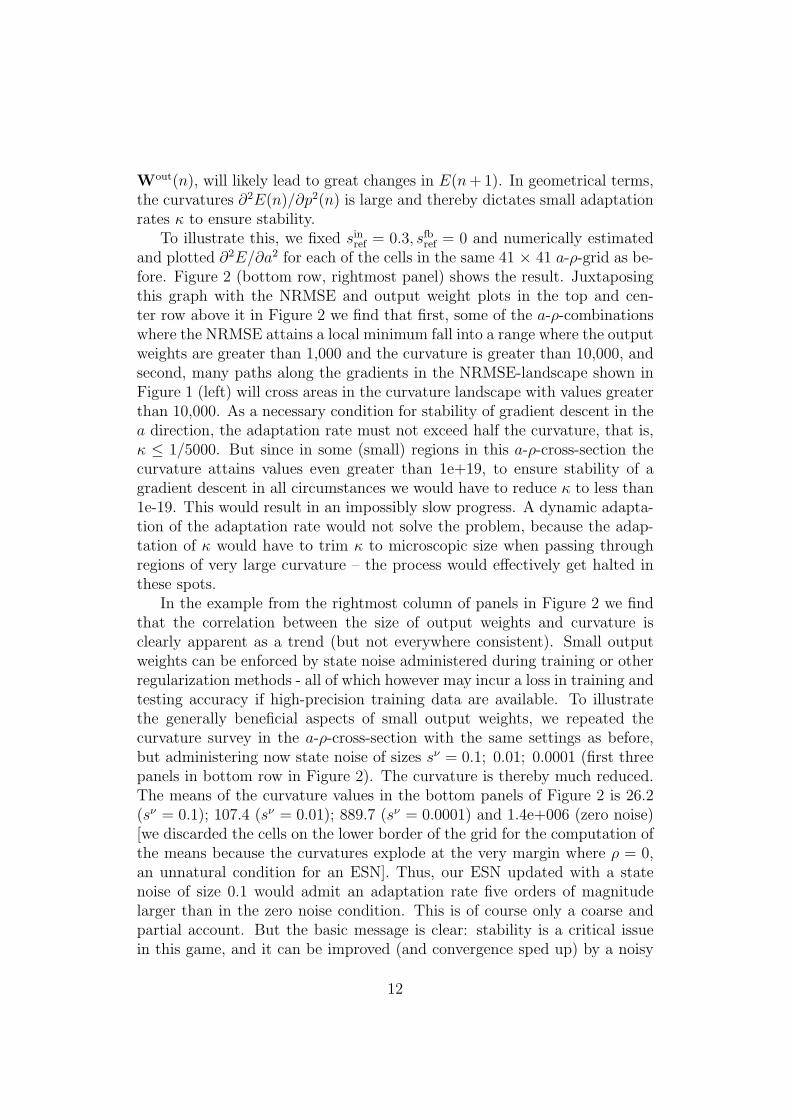
ref = 0 and numerically estimatedand plotted ∂2E/∂a2 for each of the cells in the same 41 × 41 a-ρ-grid as be-fore. Figure 2 (bottom row, rightmost panel) shows the result. Juxtaposingthis graph with the NRMSE and output weight plots in the top and cen-ter row above it in Figure 2 we find that first, some of the a-ρ-combinationswhere the NRMSE attains a local minimum fall into a range where the outputweights are greater than 1,000 and the curvature is greater than 10,000, andsecond, many paths along the gradients in the NRMSE-landscape shown inFigure 1 (left) will cross areas in the curvature landscape with values greaterthan 10,000. As a necessary condition for stability of gradient descent in thea direction, the adaptation rate must not exceed half the curvature, that is,κ ≤ 1/5000. But since in some (small) regions in this a-ρ-cross-section thecurvature attains values even greater than 1e+19, to ensure stability of agradient descent in all circumstances we would have to reduce κ to less than1e-19. This would result in an impossibly slow progress. A dynamic adapta-tion of the adaptation rate would not solve the problem, because the adap-tation of κ would have to trim κ to microscopic size when passing throughregions of very large curvature – the process would effectively get halted inthese spots.

In the example from the rightmost column of panels in Figure 2 we findthat the correlation between the size of output weights and curvature isclearly apparent as a trend (but not everywhere consistent). Small outputweights can be enforced by state noise administered during training or otherregularization methods - all of which however may incur a loss in training andtesting accuracy if high-precision training data are available. To illustratethe generally beneficial aspects of small output weights, we repeated thecurvature survey in the a-ρ-cross-section with the same settings as before,but administering now state noise of sizes sν = 0.1; 0.01; 0.0001 (first threepanels in bottom row in Figure 2). The curvature is thereby much reduced.The means of the curvature values in the bottom panels of Figure 2 is 26.2(sν = 0.1); 107.4 (sν = 0.01); 889.7 (sν = 0.0001) and 1.4e+006 (zero noise)[we discarded the cells on the lower border of the grid for the computation ofthe means because the curvatures explode at the very margin where ρ = 0,an unnatural condition for an ESN]. Thus, our ESN updated with a statenoise of size 0.1 would admit an adaptation rate five orders of magnitudelarger than in the zero noise condition. This is of course only a coarse andpartial account. But the basic message is clear: stability is a critical issuein this game, and it can be improved (and convergence sped up) by a noisy

12

black = min = 0.55


0 0.5 10

0.2

0.4

0.6

0.8

1black = min = 0.21


0 0.5 10

0.2

0.4

0.6

0.8

1black = min = 0.026


0 0.5 10

0.2

0.4

0.6

0.8



0 0.5 10

0.2

0.4

0.6

0.8

1

black = min = 0.092

white = max = 0.63(or n.d.)

0 0.5 10

0.2

0.4

0.6

0.8

1black = min = 0.36


0 0.5 10

0.2

0.4

0.6

0.8

1black = min = 0.55

white = max = 509 (or n.d.)

0 0.5 10

0.2

0.4

0.6

0.8

1black = min = 0.21white = max = 1.87e+010 (or n.d.)

0 0.5 10

0.2

0.4

0.6

0.8

1

black = min = 0.00046

white = cutoff = 100 (or n.d.)

0 0.5 10

0.2

0.4

0.6

0.8



0 0.5 10

0.2

0.4

0.6

0.8

1black = min = 1.02 max = 259960

0 0.5 10

0.2

0.4

0.6

0.8

1


black = min = 0.34max = 1.5e+19

white = cutoff = 1e+006 (or n.d.)

0 0.5 10

0.2

0.4

0.6

0.8

1

Figure 2: The multiple Sines recall task. In each panel, the x-axis is a andthe y-axis is ρ. In each row of panels, from left to right the panels correspondto state noise levels of size 0.1, 0.01, 0.0001 and 0.0. Top row: NRMSE reliefswith traces of the gradient descent algorithm at work. Center row: averageabsolute output weight sizes. Bottom row: curvatures ∂2E/∂a2. Tiny whitespeckles in some curvature plots result from rounding noise close to zero -should be black. Elevations in all surface plots are in logarithmic (base 10)scale. Several surface plots have clipped maximum height, see inset texts.

state update (or other regularizing methods that yield small output weights).In order to assess the practicality of the proposed stochastic gradient

descent method, and at the same time the impact of state noise on the modelaccuracy and the location of optimal parameters p, we ran the method fromthree starting values a/ρ = 0.33/0.2; 0.8/0.2; 0.66/0.2, in the versionwith no output feedback. To obtain meaningful graphical renderings of theresults in the a-ρ-plane, we froze sin at a value of 0.3, which was found tobe close to the optimal value in preliminary experiments. We used the “B”version of output weight adaptation. We ran the method with four statenoise levels of sν = 0.1; 0.01; 0.0001; 0.0. The corresponding adaptationrates were κ = 0.002; 0.002; 0.0002; 0.0001, and the sampling periods T forthe recomputation of the output weights were T = 1, 000; 1, 000; 100; 50.The reason for choosing smaller T in the lower-noise conditions is that the

13

output weights have to keep track of the parameter adaptation more closelydue to the greater curvature of the parameter error gradients. The methodwas run for a duration of 200,000; 200,000; 1,000,000; 1,000,000 steps in thefour conditions.

The top row in Figure 2 shows the resulting developments of a(n) andρ(n). The center row panels in the figure show the corresponding “weight-scapes”, i.e. the average absolute output weights obtained for the variousa-ρ-combinations. Progress of gradient descent is much faster in the twohigh-noise conditions (mind the different runtimes of 200,000 vs. 1 Mio steps).Attempts to speed up the low-noise trials by increasing κ led to instability.We monitored the NRMSE development of each of the gradient traces (notshown here); they all were noisily decreasing (as it should be) except for theleftmost trace in the noise-0.0001-panel. When this particular trace takesits final right turn, away from what clearly would be the downhill direction,the NRMSE starts to increase and the output weights sizes start to fluctuategreatly - a sign of impending instability.

The stochastic developments of a(n) and ρ(n) in the top row of Figure 2clearly does not follow the gradient indicated by the grayscale landscape. Thereason is that the grayshade level plots are computed by running the standardoffline learning algorithm for ESNs for each grid cell on a fixed training se-quence, whereas the gradient descent traces compute ESN output weights asthey move along, via the method “B” described above, from reservoir statesthat have been collected while the parameter adaptation proceeded. Thatis, the output weights which the gradient descent method uses are derivedfrom somewhat noisier reservoir states than the NRMSE level plots, becausein addition to the administered state noise there was parameter adaptationnoise (a remedy suggested by a reviewer would be to alternate between pe-riods where parameters p are not adjusted and states without adaptationnoise are collected for updating the output weights, and periods where pa-rameters p are stochastically adjusted with fixed output weights – we did nottry this because it would double the computational load). Furthermore, theoutput weight updates at intervals of T always “come late” with respect tothe a and ρ updates, using reservoir states which were obtained with earlier aand ρ. Thus all we should expect to learn from these graphics is whether theasymptotic values of a and ρ coincide with the minima of the error landscape– which is the case for the high-noise condition but increasingly becomes falsewith reduced noise.The compound theme of noise or other regularizers, stability, generalizationcapabilities, and size of output weights calls for further investigations. It isin our view one of the most important goals for ESN research to understandhow reservoirs can be designed or pre-trained, depending on the learning

14

task, such that small output weights will be obtained without adding statenoise or invoking other regularizers.

4 The lazy figure eight

In this section we will train a leaky integrator ESN to generate a slow “figureeight” pattern in two output neurons, and we will dynamically change thetime constant in the ESN equations to slow down and speed up the generatedpattern.

The “figure 8” generation task is a perennial exercise for RNNs (for ex-ample, see (Pearlmutter, 1995) (Zegers & Sundareshan, 2003) and referencestherein). The task appears not very complicated, because a “figure 8” can beinterpreted as the superposition of a sine (for the x direction) and a cosine ofhalf the sine’s frequency (for the y direction). However, a closer inspectionof this seemingly innocent task will reveal surprisingly challenging stabilityproblems.

Since in this section we will be speeding up and slowing down a performingESN, we use the network equation (6) as a basis. The gain γ will eventuallybe employed to set the “performance speed” of the trained ESN. Since ourfigure eight pattern will be generated on a very slow timescale, we will referto it as the “lazy eight” (L8) task.

As a teacher signal, we used a discrete-time version of the L8 trajectorywhich is centered on the origin, upright, and scaled to fill the [−1, 1] range inboth coordinate directions. One full ride along the eight uses 200 samplingpoints. Thus this signal is periodic of length 200. Periodic signals of ruggedshape and modest length (up to about 50 time points) have been trained onstandard ESNs (Jaeger, 2001) with success, but longer, smoothly and slowlychanging targets like a 200-point “lazy” eight we could never master withstandard ESNs. While low training errors can easily be achieved, the trainednets are apparently always instable when they are run in autonomous pattergeneration mode. Here is one sufficient explanation of this phenomenon(there may be more). When a standard, sigmoid-unit reservoir is drivenby a slow input signal (from the perspective of the reservoir, the feedbackfrom the output just is a kind of input), it is “adiabatically” following atrajectory along fixed point attractors of its dynamics which are defined bythe current input. If the input would freeze at a particular value, the networkstate would also freeze at the current values (reminiscent of the equilibriumpoint theory of biological motor control (Hinder & Milner, 2003).) Thisimplies that such a network cannot cope with situations like in the centercrossing of the figure 8, because, in sloppy terms, it can’t remember where it

15

came from and thus does not know where to go. Indeed, when one tries tomake a sigmoid-unit network, which had been trained on figure eight data, togenerate that trajectory autonomously, it typically goes haywire immediatelywhen it reaches the crossing point.

If in contrast we drive a leaky integrator reservoir that has a small gainγ with a slow input signal, its slow dynamics is not a forced equilibriumdynamics, but instead can memorize long-past history in its current state,so at least one reason for the failure of standard ESNs on such tasks is nolonger relevant.

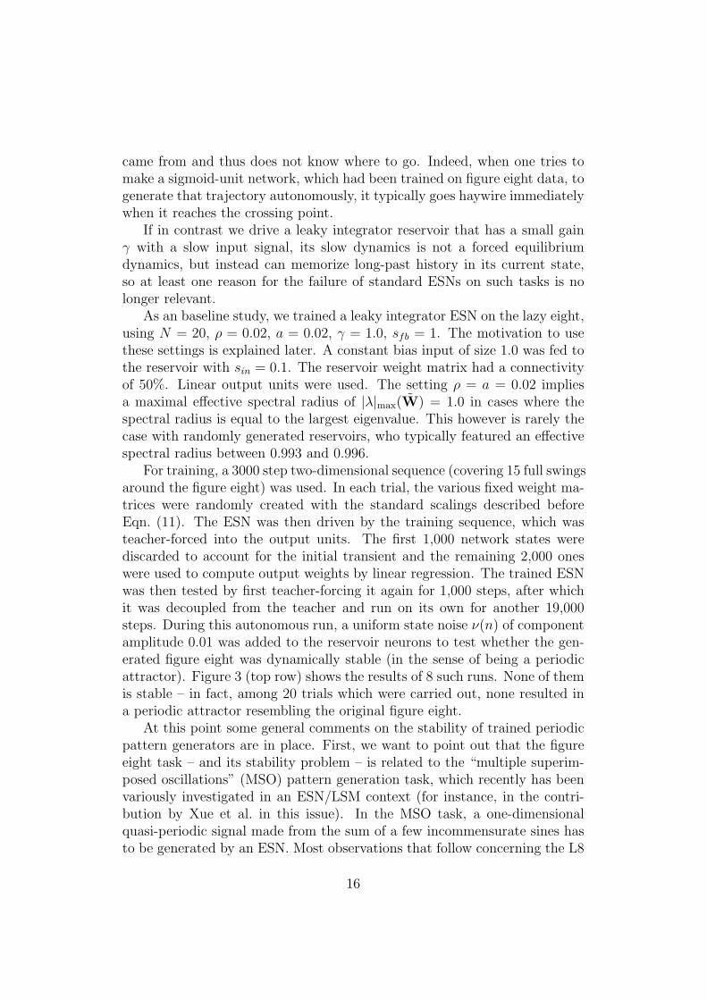
As an baseline study, we trained a leaky integrator ESN on the lazy eight,using N = 20, ρ = 0.02, a = 0.02, γ = 1.0, sfb = 1. The motivation to usethese settings is explained later. A constant bias input of size 1.0 was fed tothe reservoir with sin = 0.1. The reservoir weight matrix had a connectivityof 50%. Linear output units were used. The setting ρ = a = 0.02 impliesa maximal effective spectral radius of |λ|max(W) = 1.0 in cases where thespectral radius is equal to the largest eigenvalue. This however is rarely thecase with randomly generated reservoirs, who typically featured an effectivespectral radius between 0.993 and 0.996.

For training, a 3000 step two-dimensional sequence (covering 15 full swingsaround the figure eight) was used. In each trial, the various fixed weight ma-trices were randomly created with the standard scalings described beforeEqn. (11). The ESN was then driven by the training sequence, which wasteacher-forced into the output units. The first 1,000 network states werediscarded to account for the initial transient and the remaining 2,000 oneswere used to compute output weights by linear regression. The trained ESNwas then tested by first teacher-forcing it again for 1,000 steps, after whichit was decoupled from the teacher and run on its own for another 19,000steps. During this autonomous run, a uniform state noise ν(n) of componentamplitude 0.01 was added to the reservoir neurons to test whether the gen-erated figure eight was dynamically stable (in the sense of being a periodicattractor). Figure 3 (top row) shows the results of 8 such runs. None of themis stable – in fact, among 20 trials which were carried out, none resulted ina periodic attractor resembling the original figure eight.

At this point some general comments on the stability of trained periodicpattern generators are in place. First, we want to point out that the figureeight task – and its stability problem – is related to the “multiple superim-posed oscillations” (MSO) pattern generation task, which recently has beenvariously investigated in an ESN/LSM context (for instance, in the contri-bution by Xue et al. in this issue). In the MSO task, a one-dimensionalquasi-periodic signal made from the sum of a few incommensurate sines hasto be generated by an ESN. Most observations that follow concerning the L8

16

Figure 3: Lazy 8 test performance. Top row: baseline study, no precau-tions against instability taken. Center row: output weights computed with aridge regression regularizer. Bottom row: yield of the “noise immunization”method. Each panel shows a plot window of [−1.5, 1.5] in x and y direc-tion (stretched for plotting). The network-generated trajectory is shown asa solid black line; the gray figure 8 in the background marks the locationof the teacher eight. The three plots in each column each resulted from thesame ESN which was trained in different ways.

task pertain to the MSO task as well.Second, generating signals which are superpositions of sines is of course

simple for linear dynamical systems. It presents no difficulty to train a lin-ear ESN reservoir on the L8 or the MSO task; one will obtain training errorsclose to machine precision as long as one has at least two reservoir neuronsper sine component. When the trained network is run as a generator, one willwitness an extremely precise autonomous continuation of the target signalafter the network has been started by a short teacher-forced phase. The im-pression of perfection is however deceptive. In a linear system, the generatedsine components are not stably phase-coupled, and individually they are notasymptotically stable oscillations. In the presence of perturbations, both the

17

amplitude and the relative phase of the sine components of the generated sig-nal will go off on a random walk. This inherent lack of asymptotic stabilityis not what one would require from a pattern generation mechanism. In anESN context this implies that one has to use nonlinear reservoir dynamics(or, at least, nonlinear output units).

Third, when training nonlinear reservoir ESNs on the L8 or MSO task,one can still obtain extremely low training errors, and autonomous continu-ations of the target signal which initially look perfect. We confess that wehave ourselves been fooled by ESN generated L8 trajectories which lookedperfect for thousands of update cycles. However, when we tested our net-works for longer timespans, the process invariably at some point went havoc.Figure 4 gives an example. We suspect (and know in some cases) that asimilarly deceptive initial well-behaviour may have led other investigators ofRNN-based pattern generators to false positive beliefs about their network’sperformance.

0 1000 2000 3000 4000 5000 6000 7000 8000 9000

−5

0

5

−5 0 5−5

0

5

Figure 4: Typical behavior of naively trained L8 ESN models. The plot leftshows one of the two output signals (thick gray line: correct; thin black:network production; x-axis: update cycles) in free-running generation mode.After an initial period where the network-produced signal is all but identicalto the target, the system’s instability becomes eventually manifest by a tran-sition into an attractor unrelated to the task. Here the ultimate attractorhas an appealing butterfly shape (panel right).

Fourth, once one grows apprehensive of the stability issue, one starts tosuspect that in fact here there is a rather nontrivial challenge. On the onehand, we need a nonlinear generating system to achieve asymptotic stabil-ity. On the other hand, we cannot straightforwardly devise of the nonlineargenerator as a compound made of coupled nonlinear generators of the compo-nent sines. Coupling nonlinear oscillators of different frequencies is a delicatemaneuvre which is prone to spur interesting, but unwanted, dynamical side-effects. In other words, while the MSO and L8 signals can be seen as additivesuperpositions of sines (in a linear systems view), nonlinear oscillators do not

18

lend themselves to non-interfering “additive” couplings.In this situation, we investigated two strategies to obtain stable L8 gen-

erators. For one, following a suggestion from J. Steil we computed the out-put weights with a strong Tikhonov regularization (aka ridge regression, see(Hastie, Tibshirani, & Friedman, 2001)), using

Wout =((STS + α2I)−1 STT

)T, (27)

where S is the matrix containing the network-and-input vectors harvestedduring training in its rows, T contains the corresponding teacher vectors inits rows, and α is the regularization coefficient. For α = 0 one gets a standardlinear regression (by the Wiener-Hopf solution). We used a rather large valueof α = 1.

Our other strategy used noise to “immunize” the two component oscil-lators against interference with each other. According to this strategy, theoutput weights for the two output units were trained separately, each need-ing one run through the training data. For training the first output unit,a two-dimensional figure eight signal was prepared, which in the first com-ponent was just the original teacher d1(n), but in the second componentwas a mixture (1 − q) d2(n) + q ν(n) of the correct second figure eight sig-nal d2(n) with a noise signal ν(n). The noise signal ν(n) was created asa random permutation of the correct second signal and thus had an iden-tical average amplitude composition. The resulting two-dimensional signal(d1(n), (1 − q) d2(n) + q ν(n))T was teacher-forced on the two output unitsduring the state harvesting period. The collected states were used to com-pute output weights only for the first output unit. Then the respective rolesof the two outputs were reversed, noise was added to the first teacher andweights for the second set of output weights computed. We used a noisefraction of q = 0.2. The intuition behind this approach is that when the firstset of output weights is learnt, it is learnt from reservoir states in which theeffects of feedback from the competing second output are blurred by noise,and vice versa.

Figure 3 (center and bottom rows) illustrates the effect of these two strate-gies. We have not carried out a painstaking optimization of stability undereither strategy, and we tested only 20 randomly created ESNs. Therefore,we can only make some qualitative observations:

• Under both strategies roughly half of the 20 runs (8 and 13, respec-tively) resulted in stable generators (with state noise 0.01 for testingstability; a weaker noise might have determined a larger number ofstable runs).

19

• The ridge regression method, when it worked successfully, resulted inmore accurate renderings of the target signal than the “noise immu-nization” method.

• It is not always clear when to classify a trained generator as a successfulsolution. Deviations from the target come in many forms which appar-ently reflect different dynamical mechanisms, as can be seen from theexamples in the bottom row of Figure 3. In view of this diversity, crite-ria for accepting or rejecting a solution will depend on the applicationcontext.

To conclude this thread, we give the average training errors and averageabsolute output weight sizes for the three training setups in the followingtable.

train NRMSE stddev av. output weights stddevnaive 0.00046 0.00035 0.77 0.48regularized 0.0041 0.0019 0.039 0.010immunized 0.15 0.050 0.36 0.23

While we know how to quantify output accuracy (by MSE) in a way that lendsitself to algorithmic optimization, we do not possess a similar quantifiablecriterium for long-term stability which can be computed with comparableease, enabling us to compute a stochastic gradient online. The control pa-rameter settings sin = 0.1, sfb = 1.0, ρ = a = 0.02 were decided by a coarsemanual search using the “noise immunization” scheme. The optimizationcriterium here was long-term stability (checked by running trials), not pre-cision of short-term testing productions. While the settings for sin and sfb

appeared not to matter too much, variation in ρ and a had important ef-fects; we only came close to anything looking stable once we used very smallvalues for these two parameters. Interestingly, very small values for theseparameters also are optimal for small training MSE and testing MSE (thelatter computed only from 300-step iterated predictions without state noiseto prevent the inherent instabilities to become prominent). Figure 5 illus-trates how the training and testing error and related quantities vary witha and ρ. The main observations are that (i) throughout almost the entirea-ρ-range, small to very small NRMSEs are obtained; (ii) a clear optimimumin training and testing accuracy is located close to zero values of a and ρ– thus the values ρ = a = 0.02 which were found by aiming for stabilityalso reflect high accuracy settings; (iii) the most accurate values of a and ρcorrespond to the smallest output weights, and (iv) the curvature which isan impediment for the gradient-descent optimization schemes from Section

20

3 rises to high values as a and ρ approach their optimum region – whichwould effectivly preclude using gradient descent for localizing these optima.This combination of small output weights, high accuracy and at the sametime, high curvature, is at odds with the intuitions we developed in Section3, calling for further research.

black = min = 1.173e−005


0 0.5 10

0.2

0.4

0.6

0.8

1black = min = 1.57e−006


0 0.5 10

0.2

0.4

0.6

0.8

1black = min = 0.0188


0 0.5 10

0.2

0.4

0.6

0.8

1black = min = 0.0321

0 0.5 10

0.2

0.4

0.6

0.8

1


Figure 5: Various a-ρ-plots, similar to the plots in Section 3, for one ofthe 20-unit lazy 8 ESNs, trained with the “noise immunization” scheme.Other controls were fixed at sin = 0.1, sfb = 1.0. From left to right: (i)training NRMSE, (ii) testing NRMSE, (iii) average absolute output weights,(iv) curvature as in the bottom row of Figure 2. Grayscale coding reflectslogarithmic surface heights.

Affording the convenience of a time scale parameter γ, we finally triedout to speed up and slow down one of the “noise immunization” trainednetworks. Figure 6 (left) shows the x and y outputs obtained in a test run(with again a teacher-forced ramp-up of length 1,000, not plotted) where theoriginal γ = 1 was first slowly reduced to γ = 0.02, then held at that valuefor steps 3000 ≤ n ≤ 7000, then again increased to γ = 1.0 at n = 8500and finally to γ = 2.0 at n = 10000. The slowdown and speedup works inprinciple, but the accuracy of the resulting pattern suffers, as can be seen inFigure 6 (right). Speeding up beyond γ = 3.0 made the network lose anyvisible track of the figure 8 attractor altogether (not shown).

An inspection of Figure 6 reveals that the amplitude of the output sig-nals diminishes when γ drops, and rises again with γ beyond the correctamplitude. Our explanation rests on a generic phenomenon in discretizingdynamics with the Euler approximation: if the stepsize is increased, curva-ture of the approximated trajectories decreases. In the case of our ESNs,this means that with larger gains γ (equivalent to larger Euler stepsize) areservoir neuron’s trajectory will flatten out, and so will the generated net-work output, i.e., oscillation amplitudes grow. Using higher-order methodsfor discretizing the network dynamics would be a remedy, but the additionalimplementation and computational cost may make this inattractive.

21

−1

0

1

0 2000 4000 6000 8000 10000

−1

0

1

−2 0 2

−1

0

1

−2 0 2−2

−1

0

1

2

Figure 6: Lazy 8 slowdown/speedup performance. Left: the two generatedoutput signals (x-axis is update cycles). Center: the output figure eightgenerated by the original ESN with a constant γ = 1.0. Right: the 2-dimfigure eight plot obtained from the time-warped output signals.

5 The “Japanese Vowels” dataset

5.1 Data and task description

The “Japanese Vowels” (JV) dataset1 is a frequently used benchmark fortime series classification. The data record utterances of nine Japanese malespeakers of the vowel /ae/. Each utterance is represented by 12 LPC cep-strum coefficients. There are 30 utterances per speaker in the training set,totaling to 270 samples, and a total of 370 test samples lengths distributedunevenly over the speakers (ranging from 24 to 88 samples). The utterancesample lengths range from 7 to 29. Figure 7 gives an impression. The taskis to classify the speakers of the test samples. Various techniques have beenapplied to this problem (Kudo, Toyama, & Shimbo, 1999) (Geurts, 2001)(Barber, 2003) (Strickert, 2004). The last listed obtained the most accu-rate model known to us, a self-organizing “merge neural gas” neural networkwith 1000 neurons, yielding an error rate of 1.6% on the test data, whichcorresponds to 6 misclassifications.

5.2 Setup of experiment

We devoted a considerable effort to the JV problem. Bringing down thetest error rate to zero forced us to sharpen our intuitions about setting upESNs for classifying isolated short time series. In this subsection we not onlydescribe the setup that we finally found best, but also share our experience

1Obtainable from http://kdd.ics.uci.edu/, donated by Mineichi Kudo, JunToyama, and Masaru Shimbo

22

http://kdd.ics.uci.edu/

5 10 15 20 25

−1

0

1

2

5 10 15 20 25

−1

0

1

2

5 10 15 20 25

−1

0

1

2

5 10 15 20 25

−1

0

1

2

5 10 15 20 25

−1

0

1

2

5 10 15 20 25

−1

0

1

2

5 10 15 20 25

−1

0

1

2

5 10 15 20 25

−1

0

1

2

5 10 15 20 25

−1

0

1

2

Figure 7: Illustrative samples from the “Japanese Vowels” dataset. Threerecordings from three speakers are shown (one speaker per row). Horizontalaxis: discrete time, vertical axis: LPC cepstrum coefficients.

about setups that came out as inferior – hoping that this may save otherusers of ESNs unnecessary work.

5.2.1 Small and sharp or large and soft?

There are numerous reasonable-looking ways how one can linearly transformthe information from the input-excited reservoir into outputs representingclass hypotheses. We tried out four major variations. To provide notationfor a discussion, assume that the ith input sequence has length li, resulting inli state vectors si(1), . . . , si(li) when the reservoir is driven with this samplesequence. Here si(n) = [xi(n);ui(n)] is the extended state vector, of dimen-sion N + K, obtained by joining the reservoir state vector with the inputvector; by default we extend reservoir states with input vectors to feed theoutput units (see equation 4). From the information contained in the statessi(1), . . . , si(li) we need to somehow compute 9 class hypotheses (hi

m)m=1,...,9,giving values between 0 and 1 after inputting the ith sample to the ESN. Let(di

m)m=1,...,9 i=1,...,270 be the desired training values for the 9 output signals,that is, di

m = 1 if the ith training sample comes from the mth class, anddi

m = 0 otherwise. We tested the following alternatives to compute him:

1. Use 9 output units (ym)m=1,...,9, connect each of them to the input and

23

reservoir units by an 1 × (N + K) sized output weight vector wm,and compute wm by linear regression of the targets (di

m) on all si(n),where i = 1, . . . , 270; n = 1, . . . , li. Upon driving the trained ESN witha sequence i of length li, average each network output unit signal byputting hi

m = (∑

1≤n≤liym(n))/li. A refinement of this method, which

gave markedly better results in the JV task, is to drop a fixed numberof initial states from the extended state sequences used in training andtesting, in order to wash out the ESNs initial zero state. – Advan-tage: Simple and intuitive; would lend itself to tasks where the targettime series are not isolated but embedded in a longer background se-quence. Disadvantage: Output weights reflect a compromise betweenearly and late time points in a sequence; this will require large ESNsto enable a linear separation of classification-relevant state informa-tion from different time points. Findings: Best results (of about 2 testmisclassifications) achieved with networks of size 1,000 (about 9,000trained parameters) with regularization by state noise (Jaeger, 2002b);no clear difference between standard and leaky integrator ESNs.

2. Like before, but use only the last extended state from each sample.That is, compute wm by linear regression of the targets di

m on all si(li),where i = 1, . . . , 270. Put hi

m = ym(li). Rationale: due to the ESNsshort-term-memory capacity (Jaeger, 2002a), there is hope that thelast extended state incorporates information from earlier points in thesequence. – Advantage: Even simpler and in tune with the short-termmemory functionality of ESNs; would lend itself to usage in embed-ded target detection and classification (the situation we will encounterin section 6). Disadvantage: When there are time series of markedlydifferent lengths to cope with (which is here the case), the short-termmemory behavior of the ESN would either have to be adjusted to eachsample according to its length, or one runs danger of optimal reflec-tion of past information in the last state only for a particular length.Findings: The poorest-performing design in this list. The lowest testmisclassification numbers we could achieve were about 8 with 50-unit,leaky integrator ESNs (about 540 trainable parameters). Adjusting theshort-term memory characteristics of ESNs to sequence length by usingleaky-integrator ESNs whose gain γ was scaled inversely proportionalto the sequence length li (such that the ESN ran proportionally sloweron longer sequences) only slightly improved the training and testingclassification errors.

3. Choose a small integer D, partition each state sequence si(n) into D

24

subsequences of equal length, take the last state si(nj) from each of theD subsequences (nj = j∗li/D, j = 1, . . . , D, interpolate between statesif D is no divisor of li). This gives D extended states per sample, whichreflect a few equally spaced snapshots of the state development whenthe ESN reads a sample. Compose D collections of states for computingD sets of regression weights, where the jth collection (j = 1, . . . , D)contains the states si(nj), i = 1, . . . , 270. Use these regressions weightsto obtain for each test sample D auxiliary hypotheses hi

mj, where m =1, . . . , 9; j = 1, . . . , D. Each hi

mj is the vote of the “jth section expert”for class m. Combine these into hi

m by averaging over j. Advantage:Even small networks (order of 20 units) are capable of achieving zerotraining error, so we can hope for good models with rather few trainedparameters (e.g., D ∗ (N + K) ∗ 9 ≈ 900 for D = 3, N = 20). Thisseems promising. Disadvantage: Not transferable to embedded targetsequences. Prone to overfitting. Findings: This is the method by whichwe were first able to achieve zero training error easily. We did notexplore this method in more detail but quickly went to the techniquedescribed next, which is even sharper in the sense of needing still fewertrainable parameters for zero training error.

4. Use D segment-end-states si(nj) per sample, as before. For each train-ing sample i, concatenate them into a single joined state vector si =[si(n1); . . . ; s

i(nD)]. Use these 270 vectors to compute 9 regressionweight vectors for the 9 classes, which directly give the hi

m values.Advantage: Even smaller networks (order of 10 units) are capable ofachieving zero training error, so we can get very small models whichare sharp on the training set. Disadvantage: Same as before. Find-ings: Because this design is so sharp on the training set, but runsinto overfitting, we trimmed the reservoir size down to a mere 4 units.These tiny networks (number of trainable df’s: D ∗ (N + K) ∗ 9 ≈ 460for D = 3, N = 4) achieved the best test error rate under this de-sign option, with a bit less than 6 misclassifications, which amounts tothe current best from the literature (Strickert, 2004). Standard ESNsunder this design yielded about 1.5 times more test misclassificationsthan leaky-integrator ESNs. We attribute this to the in-built smooth-ing afforded by the integration (check Figure 7 to appreciate the jitterin the data), and to the slow timescale (relative to sample length) ofthe dominating feature dynamics, to which leaky integrator ESNs canadapt better than standard ESNs. Although the performance did notcome close to the 2 misclassifications we obtained with the first strat-egy in this list, we found this design very promising because it worked

25

already very well with tiny networks. However, something was stillmissing.

5.2.2 Combining classifiers

We spent much time on optimizing single ESNs in various setups, but neverwere able to consistently get better than 2 misclassifications. The break-through came when we joined several of the “design No. 4” networks into acombined classifier.

There are many reasonable ways of how the class hypotheses generated byindividual classifiers may be combined. Following the tentative advice givenin (Kittler, Hatef, Duin, & Matas, 1998) (Duin, 2002), we opted for the meanof the individual votes. This combination method has been found to workwell in the cited literature in cases where the individual classifiers are of thesame type and are weak, in the sense of exploiting only (random) subspaceinformation from the input data. In this scenario, vote combination by takingthe mean has been suggested because (our interpretation) it averages out thevote fluctuations that are due to the single classifiers’ biases, – hoping thatbecause the individual classifiers are of the same type, but are basing theirhypotheses on individually, randomly constituted features, the “vote cloud”centers close to the correct hypothesis.

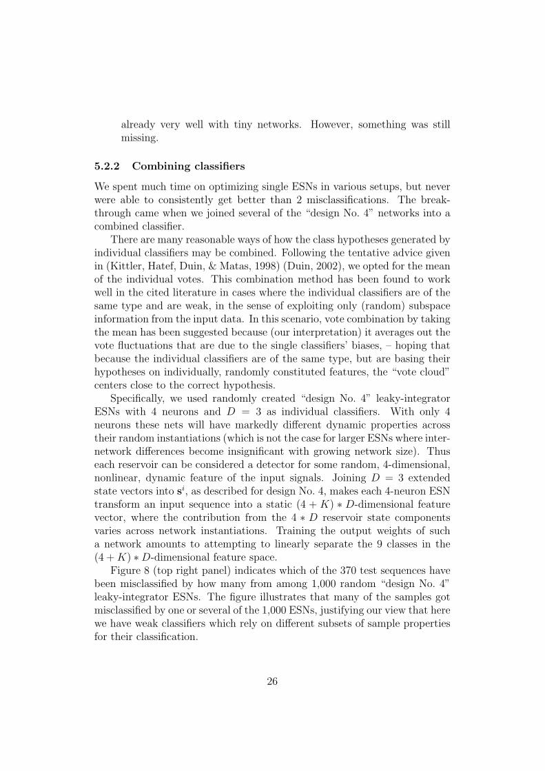
Specifically, we used randomly created “design No. 4” leaky-integratorESNs with 4 neurons and D = 3 as individual classifiers. With only 4neurons these nets will have markedly different dynamic properties acrosstheir random instantiations (which is not the case for larger ESNs where inter-network differences become insignificant with growing network size). Thuseach reservoir can be considered a detector for some random, 4-dimensional,nonlinear, dynamic feature of the input signals. Joining D = 3 extendedstate vectors into si, as described for design No. 4, makes each 4-neuron ESNtransform an input sequence into a static (4 + K) ∗ D-dimensional featurevector, where the contribution from the 4 ∗ D reservoir state componentsvaries across network instantiations. Training the output weights of sucha network amounts to attempting to linearly separate the 9 classes in the(4 + K) ∗D-dimensional feature space.

Figure 8 (top right panel) indicates which of the 370 test sequences havebeen misclassified by how many from among 1,000 random “design No. 4”leaky-integrator ESNs. The figure illustrates that many of the samples gotmisclassified by one or several of the 1,000 ESNs, justifying our view that herewe have weak classifiers which rely on different subsets of sample propertiesfor their classification.

26

5.2.3 Data preparation

We slightly transformed the raw JV data, by subtracting from each of the 12inputs the minimum value this channel took throughout all training samples.We did so because some of the inputs had a considerable systematic offset.Feeding such a signal in its raw version would amount to adding a strongbias constant to this channel, which would effectively shift the sigmoids fof reservoir units away from their centered position toward their saturationrange.

In addition to the 12 cepstrum coefficients, we always fed a constant biasinput of size 0.1. Furthermore, the input from a training or testing sequencei was augmented by one further constant Cli = li/lmaxTrain, where lmaxTrain

was the maximum among all sequence lengths in the training set. This inputis indicative of the length of the ith sequence, a piece of information that israther characteristic of some of the classes (compare Figure 7). Altogetherthis gave us 14-dimensional input vectors.

5.2.4 Optimizing global parameters

We used the network update equation (11) for this case study and thus hadto optimize the global parameters N , a, ρ, sin, and sν . Because our gradientdescent optimization does not yet cover nonstationary, short time series, wehad to resort to manual experimentation to optimize these. To say the truth,we relied very much on our general confidence that ESN performance is quiterobust with respect to changes in global control parameters, and investedsome care only in the optimization of the leaking rate a, whereas the otherparameters were settled in a rather offhand fashion.

To use a network size of N = 4 was an ad-hoc decision after observingthat individual nets with N = 10 exhibited significant overfitting. We didnot try any other network size below 10.

The input scaling was kept at a value of sin = 1.5 from the preliminaryexperiments which we briefly pointed out before. Likewise, the spectral ra-dius was just kept from our preliminary attempts with single-ESN modelsat a value of ρ = 0.2 . We did not insert any state noise (that is, we usedsν = 0) because stability was not at stake in the absence of output feedback;because the data were noisy in themselves; and because the output weightswe obtained were moderately sized (typical absolute sizes averaged between1 and 10, with a large variation between individual ESNs).

In order to find a good value for a, we carried out a tenfold cross-validationon the training data for various values of a, for 25 independently created 4-unit ESNs. Figure 8 (top left) shows the findings for a = 0.1, 0.15, . . . , 0.5.

27

Error bars indicate the NRMSE standard deviation across the 25 individualESNs. This outcome made us choose a value of a = 0.2. As we will see,this NRMSE is very nonlinearly connected to the ultimate classification per-formance, and small improvements in NRMSE may give a large benefit inclassification accuracy.

5.2.5 Details of network configuration

We used output units with the tanh squashing function. We linearly trans-formed the 0-1-teacher values by 0 7→ −0.8, 1 7→ 0.8 to exploit the rangeof this squashing function (for NRMSE calculations and plots we undid thistransformation wherever network output values were concerned). The reser-voir and input connection weight matrices were fully connected, with entriesdrawn from a uniform distribution over [−1, 1]. The reservoir weight matrixW was subsequently scaled to a spectral radius of 1, to be scaled by ρ = 0.2in our update equation (11). In each run of a network with a training ortesting sample, the initial network state was zero.

0.1 0.2 0.3 0.4 0.50.31

0.32

0.33

0.34

a

NR

MS

E

0 100 200 300 4000

1

2

3

test sample Nr

log 10

(Nr

of m

iscl

ass.

+ 1

)

1 5 10 20 50 100 200 50010000.2

0.25

0.3

0.35

0.4

Nr of combined classifiers

NR

MS

E

NRMSE trainNRMSE test

1 5 10 20 50 100 200 5001000−2

0

2

4

6

Nr of combined classifiers

Nr

of m

iscl

ass. MisClass train

MisClass test

Figure 8: Diagnostics of the JV task. Top left: cross-validation NRMSE foroptimizing the leaking rate a. Top right: Distribution of misclassified testsamples, summed over 1,000 individual nets. y-scaling is logarithmic to basee. Bottom left: average NRMSE for varying Nrs of combined ESNs. Errorbars indicate stddev. Bottom right: Average test misclassifications. Again,error bars indicate stddev. For details see text.

28

5.3 Results

We trained 1,000 4-neuron ESNs individually on the training data, thenpartitioned the trained networks into sets of size 1, 2, 5, 10, 20, 50, 100,200, 500, 1000, obtaining 1,000 individual classifiers, 500 classifiers whichcombined 2 ESNs, etc., up to one combined classifer made from all 1,000ESNs.

Figure 8 comprises the performance we observed for these classifiers. Theaverage number of test misclassifications for individual ESNs was about 5.4with a surprisingly small standard deviation. It dropped below 1.0 when 20ESNs were combined, then steadily went down further until zero misclas-sifications was reached by the collectives sized 500 and 1,000. The meantraining misclassification number was always exactly 1 except for the indi-vidual ESNs. An inspection of data revealed that it was always the sametraining sample (incidentally, the last of the 270) which was misclassified.

6 Time warping invariant echo state networks

Time warping of input patterns is a common problem when recognizing hu-man generated input or dealing with data artificially transformed into timeseries. The most widely used technique for dealing with time-warped patternsis probably dynamic time warping (DTW) (Itakura, 1975) and its modifica-tions. It is based on finding the cheapest (w.r.t. some cost function) mappingbetween the observed signal and a prototype pattern. The price of the map-ping is then taken as a classification criterion. Another common approachto time-warped recognition uses hidden Markov models (HMMs) (Rabiner,1990). The core idea here is that HMMs can “idle” in a hidden state and thusadapt to changes in the speed of an input signal. An interesting approachof combining HMMs and neural networks is proposed in (Levin, Pieraccini,& Bocchieri, 1992), where neurons that time-warp their input to match it toits weights optimally are introduced.

A simple way of directly applying RNNs for time-warped time series clas-sification was presented in Sun, Chen, and Lee (1993). We take up the basicidea from that work to derive an effective method for dynamic recognition oftime-warped patterns, based on leaky-integrator ESNs.

29

6.1 Time warping invariance

Intuitively, time warping can be understood as variations in the “speed” of aprocess. For discrete-time signals obtained by sampling from a continuous-time series it can alternatively be understood as variation in the samplingrate. By definition two signals α(t) and β(t) are connected by an approximatecontinuous time warping (τ1, τ2), if τ1, τ2 are strictly increasing functions on[0, T ], and α(τ1(t)) ∼= β(τ2(t)) for 0 ≤ t ≤ T . We can choose one signal, sayα(t), as a reference and all signals that are connected with it by some timewarping (e.g. β(t)) call (time-)warped versions of α(t). We will also refer toa time warping (τ1, τ2) as a single time warping (function) τ(t) = τ2(τ

−11 (t))

which connects the two time series by β(t) = α(τ(t)).We will deal with the problem of recognition (detection plus classification)

of time-warped patterns in a background signal, and follow the approachoriginally proposed in (Sun et al., 1993). This method does not look for a timewarping that could map an observed signal to a target pattern. Time warpinginvariance is achieved by normalizing time dependence of the state variableswith respect to the length of trajectory of the input signal in its phase space.In other words, the input signal is considered in a “pseudo-time” domain,where “time span” between two subsequent pseudo time steps is proportionalto the metric distance in the input signal between these time steps. As aconsequence, input signals will be changing with a constant metric rate inthis “pseudo-time” domain. In continuous time, for a k-dimensional inputsignal u(t), u : R+ → Rk we can define such a time warping τ ′u : R+ → R+

by

dτ ′u(t)/dt = b · ‖du(t)/dt‖ , (28)

where b is a constant factor. Note, that the time warping function τ ′u de-pends on the signal u which it is warping. Then the signal warped by τ ′u(i.e. in the “pseudo-time” domain) becomes u(τ ′u(t)), and as a consequence‖du(τ ′u(t))/dt‖ = 1/b, i.e. the k-dimensional input vector u(τ ′u(t)) changeswith a constant metric rate equal to 1/b in this domain. Furthermore, if twosignals u1(t) and u2(t) are connected by a time warping τ , then time warpingthem with τ ′u1

and τ ′u2respectively results in u1(τ

′u1

(t)) = u2(τ′u2

(t)), whichis what we mean by time warping invariance (see Figure 9 for the graphicalinterpretation of the k = 1 case).

A continuous-time processing device governed by an ODE with a timeconstant c could be made invariant against time warping in its input signalu(t), if for any given input it could vary its processing speed according to τ ′u(t)by changing the time constant c in the equations describing its dynamics.This is an alternative to time-un-warping the input signal u(t) itself. Leaky

30

0 20 40 60 80 100 120−0.2

−0.1

0

0.1

0.2

time n

u(n)

No time warping, l = 0

0 20 40 60 80 100 120−0.2

−0.1

0

0.1

0.2

"pseudotime" τ’u(n)

u(τ’ u(n

))

↓ time warping invariant interpretation ↓

0 20 40 60 80 100 120−0.2

−0.1

0

0.1

0.2

time n

u(n)

Time warping l = 0.7

0 20 40 60 80 100 120−0.2

−0.1

0

0.1

0.2

"pseudotime" τ’u(n)

u(τ’ u(n

))

↓ time warping invariant interpretation ↓

≠

≈

Figure 9: A time warping invariant interpretation of two one-dimensional sig-nals connected by a time warping. Top left: reference signal with l = 0. Topright: a version of the same with l = 0.7. Bottom panels: transformationsfrom the top panel sequences into the “pseudotime” domain τ ′u(n) accordingto (28). We can observe that for one-dimensional signals the transformationto warping-invariant pseudo-time causes a significant loss of information –the signal u(τ ′u(n)) can be fully described by the sequence of values at localminimums and maximums of u(n).

integrator neurons offer their service at this point. Considering first thecontinuous-time version of leaky-integrator neurons (equation (1)), we woulduse the inverse time constant 1/c to speed up and slow down the network,by making it time-varying according to (28). Concretely, we would set

c(t) = (b · ‖du(t)/dt‖)−1 (29)

If we have discrete sampled input u(n), we use the discrete-time approxima-tion from equation (6) and make the gain γ time-varying by

γ(n) = b · ‖u(n)− u(n− 1)‖ . (30)

6.2 Data, learning task, and ESN setup

We prepared continuous-time time series of various dimensions, consistingof a red-noise background signal into which many copies of a short target

31

pattern were smoothly embedded. The task is to recognize the target pat-tern in the presence of various degrees of time warping applied to the inputsequences.

Specifically, a red-noise background signal g(t) was obtained by filteringout 60% of the higher frequencies from a [−0.5, 0.5]k uniformly distributedwhite noise signal. A short target sequence p(t) of duration Tp with a sim-ilar frequency makeup was generated and smoothly embedded into g(t) atrandom locations, using suitable soft windowing techniques for the embed-ding to make sure that no novel (high) frequency components were created inthe process (details in Lukosevicius et al. (2006)). This embedding yieldedcontinuous-time input signals u(t) which were subsequently sampled andtime-warped to obtain discrete-time inputs u(n).

The (1-dimensional) desired output signal d(t) was constructed by placingnarrow Gaussians on a background zero signal, at the times where the targetpatterns end. The height of the Gaussians is scaled to 1. Figure 10 gives animpression of our data.

0 50 100 150 200 250 300 350 400−0.2

−0.1

0

0.1

0.2No time warping, l = 0

0 50 100 150 200 250 300 350 400−0.2

−0.1

0

0.1

0.2

n

Time warping l = 0.7 yteacher(n) u(n)

Figure 10: A fragment of a one-dimensional input and corresponding teachersignal without and with time warping.

Discrete time time-warped observations u(n) of the process u(t) weredrawn as u(n) = u(τ(n)), where τ : N → R+ fulfilled both time warping anddiscretization functions. Both u(t) and the corresponding teacher d(t) werediscretized/time-warped together. More specifically, we used

τ(n) = (n + 10 · l sin(0.1n)), (31)

where l ∈ [0, 1] is the level of time warping: τ(n) is a straight line (no timewarping) when l = 0, and is a nondecreasing function as long as l ≤ 1. In the

32

extreme case of l = 1, time “stands still” at some points in the trajectory. Inthe obtained signals u(n) the pattern duration Tp on average correspondedto 20 time steps.

The learning task for the ESN is to predict d(n) from u(n). In eachnetwork-training-testing trial, the warping level l on the training data wasthe same as on the test data. Training sequences were of length 3,000, ofwhich the first 1,000 were discarded before computing the output weights inorder to wash out initial network transients. For testing, sequences of length500 were used throughout.

We used leaky-integrator ESNs with 50 units. The reservoir weight matrixwas randomly created with a connectivity of 20%; nonzero weights weredrawn from a uniform distribution centered on 0 and then globally rescaled toyield a reservoir weight matrix W with unit spectral radius. We augmentedinputs u(n) by an additional constant bias signal of size 0.01, yielding aK = k + 1 dimensional input overall. Input weights were randomly sampledfrom a uniform distribution over [−1, 1]. There were no output feedbacks.

The spectral radius ρ and the leaking rate a were manually optimized tovalues of ρ = 0.3, a = 0.3 on inputs without time-warping. Likewise, on datawithout time-warping we determined by manual search an optimal referencevalue for the gain of γ0 = 1.2.

Turning to time-warped data, for each time series we set the constantb from (28) such that on average a gain of 〈γ(n)〉 = 1.2 would result fromrunning the ESN with a dynamic gain according to (30), that is, for a giveninput sequence we put

b = 1.2/〈‖u(n)− u(n− 1)‖〉. (32)

This results in the following update equation:

x(n + 1) = (1− aγ(n)) x(n) + γ(n) f(Winu(n + 1) + Wx(n)), (33)

where γ(n) = b · ‖u(n)− u(n− 1)‖. As a safety catch, the range of γ(n) wasbounded by a hard limit to satisfy the constraint from equation (5), that is,γ(n) was limited to values of at most 1/a.

6.3 Results

We compared the performance of three types of ESNs: (i) leaky integra-tor ESNs with fixed γ = 1.2; (ii) time-warping-invariant ESNs (TWIESNs)according to equation (28); and for comparison we also constructed (iii) aversion of a leaky integrator ESNs which unwarped the signals in an optimal

33

way, using the information (which in real life is unavailable) of the time warp-ing τ : this ESN version has γ(n) externally set to min(b[τ(n)−τ(n−1)], 1/a).Let us call this type of networks, “oracle” ESNs.

For each run, we computed two performance criteria: the NRMSE of net-work output vs. d(n), and the ratio of q of correctly recognized targets. Todetermine q, each connected interval of n for which y(n) > h correspondsto one claimed target recognition. Any such event is considered a correctrecognition if the intervals of n where y(n) > h and yteacher(n) > h overlap.The value of h was optimized by maximizing q over the training data. Then,q is evaluated as Nr. of correct recognitions / (Nr. of targets in test sequence+ Nr. of claimed recognitions − Nr. of correct recognitions). Figure 11 sum-marizes the findings for k = 1, 3, 10, 30. Each plot renders the average valuesfrom 100 runs with independently created ESNs.

The main observations are the following.

• If k and l are small, the fixed leaky integrator ESNs do better thanTWIESNs. This can be explained by the loss of temporal informationinduced by the transformation to pseudotime.

• If k or l is large, TWIESNs outperform fixed leaky integrator ESNs, andindeed come close to oracle ESNs when k is 10 or larger. This meansthat the purely temporal information contributes little to the recog-nizability of patterns, as opposed to the “structural” (time-scaling-invariant) information in the input sequences. Since in real-life appli-cations where time warping is an issue (for instance, speech or hand-writing recognition), inputs are typically feature vectors of sizes beyond10, our approach seems to hold some promise.

• NRMSE and recognition rate q remain almost, but not quite constantfor TWIESNs as l varies from zero to one. Naively, one should expectthat q is not affected at all by l, because TWIESNs should “see” inden-tical pseudo-time series across all l, as in the bottom panels of Figure9. Indeed, this is not exactly the case: when γ(n) becomes large, thereservoir dynamics is not an exact sped-up version of a slower dynam-ics, due to inaccuracies of the Euler discretization. This explains thesystematic, slight increase in NRMSE as l grows. A remedy wouldbe to use higher-order discrete approximations of the continuous-timeleaky integrator dynamics from (1), for instance Runge-Kutta approx-imations.

34

0 0.2 0.4 0.6 0.8 10.4

0.6

0.8

1

1.2

1.4

Nor

mal

ized

MS

E

k = 1

0 0.2 0.4 0.6 0.8 10

0.2

0.4

0.6

0.8

Qua

lity

of r

ecog

nitio

n q

0 0.2 0.4 0.6 0.8 10.2

0.4

0.6

0.8

1k = 3

0 0.2 0.4 0.6 0.8 10

0.2

0.4

0.6

0.8

1

0 0.2 0.4 0.6 0.8 10.2

0.4

0.6

0.8

1

Nor

mal

ized

MS

E

k = 10

0 0.2 0.4 0.6 0.8 10.2

0.4

0.6

0.8

1

Level of time warping l

Qua

lity

of r

ecog

nitio

n q

0 0.2 0.4 0.6 0.8 10.2

0.4

0.6

0.8

1k = 30

0 0.2 0.4 0.6 0.8 1

0.7

0.8

0.9

1

Level of time warping l

classical ESN TWIESN explicit time "unwarping"

Figure 11: Performance of fixed-γ ESNs (dashed), oracle ESNs (dotted) andTWIESNs (solid), for input dimensions k = 1, 3, 10 and 30, and differentlevels of time warping l (x-axes). Bold lines: test performance, thin lines:performance on training data. For details see text.

7 Conclusion

Leaky integrator ESNs are only slightly more complicated to implement andto use than standard ESNs and appear to us as quite flexible devices whentimescale phenomena are involved, where standard ESNs run into difficul-ties. Caution is however advised when simple Euler approximations to thecontinuous-time leaky integrator dynamics are used.

Two questions were encountered which we consider to be of longer-lastingimportance:

• Find computationally efficient ways to optimize the global scaling pa-rameters of ESNs. Specifically, naive stochastic gradient descent ap-proaches, as introduced in this paper, suffer from poor stability prop-

35

erties, which renders them impractical in many cases.

• Analyse conditions and provide practical training schemes that ensurestability of ESNs trained as complex pattern generators.

Finally we want to point out a question which we think would concern anymodeling approach to nonlinear dynamics, whether based on RNNs or not.Humans can to some extent adjust the speed (and amplitude) of generatedmotor (or vocal) trajectories. For instance, they can speak faster or slower,or perform a gesture at different velocity. What could an underlying neu-ral mechanism be? We can’t think of a biologically plausible mechanism bywhich biological brains could dynamically adjust the physical time constantsof their neurons in a quick, adaptive, and homogeneous fashion, in the waywe can adjust γ in our equations. However, biological brains can apparentlyadjust gains of neural connection pathways. It would be an interesting chal-lenge for theoretical neuroscience to devise of dynamical or RNN mechanismsby which trajectories can be sped up or slowed down, not by directly changingtime constants but instead by changing connection (coupling) gains.

A Proof of proposition 1

For any two states x(n),x′(n) the following holds:

‖x(n)− x′(n)‖ =

= ‖(1− aδ

c)(x(n)− x′(n)) +

+δ

c

(f(Winu(n + 1) + Wx(n))− f(Winu(n + 1) + Wx′(n))

)‖

≤ (1− aδ

c)‖x(n)− x′(n)‖+

+δ

c‖f(Winu(n + 1) + Wx(n))− f(Winu(n + 1) + Wx′(n))‖

≤ (1− aδ

c)‖x(n)− x′(n)‖+

δ

c‖Wx(n)−Wx′(n)‖

≤ (1− δ

c(a− σmax)) ‖x(n)− x′(n)‖

Thus, |1 − δc

(a − σmax)| is a global Lipschitz rate by which any two statesapproach each other in a network update.

36

Acknowledgments

The work on time warping invariant ESNs reported here was supported bystudent contract grants for ML and DP from Planet intelligent systemsGmbH, Raben Steinfeld, Germany. The authors would also like to thankfive (!) anonymous reviewers of the NIPS 2005 conference, who helped toimprove the presentation of Section 6, which once was a NIPS submission.The treatment of the lazy eight task owes much to discussions with J. Steil,R. Linsker, J. Principe and B. Schrauwen. The authors also express theirgratitude toward two anonymous reviewers of the Neural Networks Journalfor detailed and helpful commentaries. International patents for the basicESN architecture and training algorithms have been claimed by FraunhoferIAIS www.iais.fraunhofer.de.

References

Barber, D. (2003). Dynamic Bayesian networks with deterministic latent ta-bles. In Proc. NIPS 2003. (http://www.anc.ed.ac.uk/∼dbarber/publi-cations/barber nips dethidden.pdf)

Buehner, M., & Young, P. (2006). A tighter bound for the echo state property.IEEE Transactions on Neural Networks, 17 (3), 820- 824.

Buonomano, D. V. (2005). A learning rule for the emergenceof stable dynamics and timing in recurrent networks. Jour-nal of Neurophysiology, 94, 2275-2283. (http://www.neuro-bio.ucla.edu/∼dbuono/BuonoJNphy05.pdf)

Duin, R. P. W. (2002). The combining classifier: To train or notto train? In R. Kasturi, D. Laurendeau, & C. Suen (Eds.),Proceedings 16th International Conference on Pattern Recognition(ICPR16), vol. II (p. 765-770). IEEE Computer Society Press.(http://ict.ewi.tudelft.nl/∼duin/papers/icpr 02 trainedcc.pdf)

Farhang-Boroujeny, B. (1998). Adaptive filters: Theory and applications.Wiley.

Geurts, P. (2001). Pattern extraction for time series classification.In L. De Raedt & A. Siebes (Eds.), Proc. PKDD 2001 (p. 115-127). (http://www.montefiore.ulg.ac.be/∼geurts/publications/geurts-pkdd2001.pdf)

37

www.iais.fraunhofer.de

Hastie, T., Tibshirani, R., & Friedman, J. (2001). The elements of statisticallearning. Springer Verlag.

Hinder, M. R., & Milner, T. E. (2003). The case for an internal dynam-ics model versus equilibrium point control in human movement. J.Physiol., 549 (3), 953-963. (http://www.sfu.ca/∼tmilner/953.pdf)

Itakura, F. (1975). Minimum prediction residual principle applied to speechrecognition. IEEE Transactions on Acoustics, Speech and Signal Pro-cessing, 23 (1), 67–72.

Jaeger, H. (2001). The ”echo state” approach to analysing and training recur-rent neural networks (GMD Report No. 148). GMD - German NationalResearch Institute for Computer Science. (http://www.faculty.iu-bremen.de/hjaeger/pubs/EchoStatesTechRep.pdf)

Jaeger, H. (2002a). Short term memory in echo state networks(GMD-Report No. 152). GMD - German National Research Insti-tute for Computer Science. (http://www.faculty.iu-bremen.de/hjae-ger/pubs/STMEchoStatesTechRep.pdf.)

Jaeger, H. (2002b). Tutorial on training recurrent neural networks, cover-ing BPPT, RTRL, EKF and the echo state network approach (GMDReport No. 159). Fraunhofer Institute AIS. (http://www.faculty.iu-bremen.de/hjaeger/pubs/ESNTutorial.pdf)

Jaeger, H. (2003). Adaptive nonlinear system identification with echostate networks. In S. Becker, S. Thrun, & K. Obermayer (Eds.),Advances in Neural Information Processing Systems 15 (p. 593-600).MIT Press, Cambridge, MA. (http://www.faculty.iu-bremen.de/hjae-ger/pubs/esn NIPS02)

Jaeger, H., & Haas, H. (2004). Harnessing nonlinearity: Predict-ing chaotic systems and saving energy in wireless communica-tion. Science, 304, 78-80. (http://www.faculty.iu-bremen.de/hjae-ger/pubs/ESNScience04.pdf)

Kittler, J., Hatef, M., Duin, R., & Matas, J. (1998). On combin-ing classifiers. IEEE Transactions on Pattern Analysis and Ma-chine Intelligence, 20 (3), 226-239. (http://ict.ewi.tudelft.nl/∼duin/pa-pers/pami 98 ccomb.pdf)

38

Kudo, M., Toyama, J., & Shimbo, M. (1999). Multidimensional curve clas-sification using passing-through regions. Pattern Recognition Letters,20 (11), 1103-1111.

Levin, E., Pieraccini, R., & Bocchieri, E. (1992). Time-warping network:A hybrid framework for speech recognition. In Advances in NeuralInformation Processing Systems 4, [NIPS Conference] (pp. 151–158).

Lukosevicius, M., Popovici, D., Jaeger, H., & Siewert, U. (2006). Timewarping invariant echo state networks (IUB Technical Report No. 2).International University Bremen. (http://www.iu-bremen.de/im-peria/md/content/groups/research/techreports/twiesn iubtechre-port.pdf.)

Maass, W., Joshi, P., & Sontag, E. (2006). Computational aspects offeedback in neural circuits. PLOS Computational Biology, in press.(http://www.igi.tugraz.at/maass/psfiles/168 v6web.pdf)

Maass, W., Natschlaeger, T., & Markram, H. (2002). Real-time com-puting without stable states: A new framework for neural computa-tion based on perturbations. Neural Computation, 14 (11), 2531-2560.(http://www.cis.tugraz.at/igi/maass/psfiles/LSM-v106.pdf)

Mauk, M., & Buonomano, D. (2004). The neural basis of temporal process-ing. Annu. Rev. Neurosci., 27, 307-340.

M.C., Xu, D., & Principe, J. (accepted 2006). Analysis and design of echostate networks for function approximation. Neural Computation, toappear.

Pearlmutter, B. (1995). Gradient calculation for dynamic recurrent neuralnetworks: a survey. IEEE Trans. on Neural Networks, 6 (5), 1212-1228.(http://www.bcl.hamilton.ie/∼bap/papers/ieee-dynnn-draft.ps.gz)

Rabiner, L. (1990). A tutorial on hidden Markov models and selected appli-cations in speech recognition. In A. Waibel & K.-F. Lee (Eds.), Read-ings in speech recognition (p. 267-296). Morgan Kaufmann, San Mateo.(Reprinted from Proceedings of the IEEE 77 (2), 257-286 (1989))

Schiller, U., & Steil, J. J. (2005). Analyzing the weight dynam-ics of recurrent learning algorithms. Neurocomputing, 63C, 5-23.(http://www.techfak.uni-bielefeld.de/∼jsteil/publications.html)

39

Schmidhuber, J., Gomez, F., Wierstra, D., & Gagliolo, M. (2006, in press).Training recurrent networks by evolino. Neural Computation.

Stanley, G., Li, F., & Dan, Y. (1999). Reconstruction of natural scenes fromensemble responses in the lateral genicualate nucleus. J. Neurosci.,19 (18), 8036-8042. (http://people.deas.harvard.edu/∼gstanley/publi-cations/stanley dan 1999.pdf)

Strickert, M. (2004). Self-organizing neural networks for sequenceprocessing. Phd thesis, Univ. of Osnabruck, Dpt. of Com-puter Science. (http://elib.ub.uni-osnabrueck.de/publications/diss/E-Diss384 thesis.pdf)

Sun, G.-Z., Chen, H.-H., & Lee, Y.-C. (1993). Time warping invariant neuralnetworks. In Advances in Neural Information Processing Systems 5,[NIPS Conference] (pp. 180–187). San Francisco, CA, USA: MorganKaufmann Publishers Inc.

Zant, T. van der, Becanovic, V., Ishii, K., Kobialka, H.-U., & Ploger,P. (2004). Finding good echo state networks to control an un-derwater robot using evolutionary computations. In CD-ROM Proc.IAV 2004 - The 5th Symposium on Intelligent Autonomous Ve-hicles. (http://www.ais.fraunhofer.de/∼vlatko/Publications/Fin-ding good esn FINAL PhotoCopyReady.pdf)

Zegers, P., & Sundareshan, M. K. (2003). Trajectory generation and mod-ulation using dynamic neural networks. IEEE Transactions on NeuralNetworks, 14 (3), 520 - 533.

40

optimization and applications of echo state networks with

Documents