optimisation of chromatography for downstream …discovery.ucl.ac.uk/1334599/1/1334599.pdf ·...
TRANSCRIPT

UNIVERSITY COLLEGE LONDON
Optimisation of
Chromatography for
Downstream Protein
Processing
Eleftheria Polykarpou
A thesis submitted in fulfillment for the
degree of Doctor of Philosophy
in the
Department of Biochemical Engineering
November 2011

Declaration of Authorship
I, Eleftheria Polykarpou, declare that this thesis titled, ‘Optimisation
of Chromatography for Downstream Protein Processing’ and the work
presented in it are my own. I confirm that:
� This work was done wholly while in candidature for a research
degree at University College London.
� Where any part of this thesis has previously been submitted for
a degree or any other qualification at this University or any other
institution, this has been clearly stated.
� Where I have consulted the published work of others, this is al-
ways clearly attributed.
� Where I have quoted from the work of others, the source is al-
ways given. With the exception of such quotations, this thesis is
entirely my own work.
� I have acknowledged all main sources of help.
� Where the thesis is based on work done by myself jointly with
others, I have made clear exactly what was done by others and
what I have contributed myself.
Signed:
Date:
1

Στη µητ ερα µoυ και τoν πατ ερα µoυ
2

Acknowledgements
I would like to express my deepest gratitude for the help and guidance
received by my supervisors Paul A. Dalby and Lazaros G. Papageor-
giou, especially acknowledging our regular discussions with Lazaros G.
Papageorgiou, without whom this work could not have culminated in
such a result.
I am certainly indebted to many people who have helped in various
ways throughout; Giovanna for introducing me to PhD life, Melanie
for her valuable help in learning to speak LaTeX and Spanish, Sunil
Chhatre for his help in understanding the theory of chromatography in
depth, Songsong for his expertise in GAMS, Nouri Samsatli for guiding
me through using gPROMS, and many others who I’ve collaborated
with over the last few years.
Especially those with which I have had the privilege to interact past
working constraints and become good friends with, hold a most signif-
icant optimising factor of PhD life in London. “Los pinches” Alberto,
Miguel and Shane offered amazing times along beer sessions in ULU,
and of course Giovanna, Melanie and Chandni made every day so much
more than just a working environment. And the later intakes of the
PPSE (former CAPE) room Di, Mozhdeh, Ozlem and Shirin, unex-
pectedly maintained the warmth of having endless discussions about
science, life and other diversely interesting issues. Thank you all for
being great friends.
Avgoustine, Mitso and Niki, thank you for the many beautiful moments
shared together during our time in London (under the same roof or sail
at times) and last but not least, Apostoli for sharing and completing
yet another experience!
This work was carried out, under the Innovative Manufacturing Re-
search Council and their financial assistance is greatly acknowledged.
3

On ne peut vivre que le present...

Abstract
Downstream bioprocessing and especially chromatographic steps, com-
monly used for the purification of multicomponent systems, are signif-
icant cost drivers in the production of therapeutic proteins. Lately,
there has been an increased interest in the development of systematic
methods where operating conditions are defined and chromatographic
trains are selected.
Several models have been developed previously, where chromatographic
trains were selected under the assumption of 100 % recovery of the
desired product. Removing this assumption gives the opportunity not
only to select chromatographic trains but also determine the timeline
in which the product is selected.
Initially, a mixed integer non-linear (MINLP) programming mathemat-
ical model was developed to tackle that problem and was tested using
three illustrative examples. Later on, this model was linearised by ap-
plying piecewise linear approximation techniques and computational ef-
ficiency was improved. Next, an alternative MILP model was developed
by discretising the recovery levels of the product and computational ef-
ficiency improved even by 100-fold. Finally, the equilibrium dispersive
model was used in a simple 4-protein mixture and the MINLP model
was validated.
This research represents a significant step towards efficient downstream
process operation and synthesis.

Contents
Declaration of Authorship 1
Acknowledgements 3
Abstract 5
List of Figures 10
List of Tables 12
Symbols 14
1 Introduction and theoretical background 18
1.1 Scope . . . . . . . . . . . . . . . . . . . . . . . . . . . . 18
1.2 Biopharmaceutical industry . . . . . . . . . . . . . . . . 19
1.3 Typical flowsheet . . . . . . . . . . . . . . . . . . . . . . 21
1.4 Chromatography . . . . . . . . . . . . . . . . . . . . . . 22
1.4.1 History of chromatography . . . . . . . . . . . . . 22
1.4.2 How does chromatography work? . . . . . . . . . 23
1.5 Types of chromatographic separation . . . . . . . . . . . 25
1.5.1 Nature of mobile and stationary phase . . . . . . 25
1.5.2 Scale of operation . . . . . . . . . . . . . . . . . . 25
1.5.3 Modes of operation . . . . . . . . . . . . . . . . . 26
1.6 Principles of separation . . . . . . . . . . . . . . . . . . . 29
1.7 Aims and objectives . . . . . . . . . . . . . . . . . . . . 36
1.8 Outline of the thesis . . . . . . . . . . . . . . . . . . . . 36
2 Literature Review 38
2.1 Drivers for change . . . . . . . . . . . . . . . . . . . . . . 38
6

2.2 Operation of chromatographic processes . . . . . . . . . 39
2.2.1 Protein structure approaches . . . . . . . . . . . . 41
2.2.2 Mechanistic approaches . . . . . . . . . . . . . . . 41
2.2.3 Graphical approaches . . . . . . . . . . . . . . . . 43
2.2.4 Black-box approaches . . . . . . . . . . . . . . . . 44
2.3 Synthesis of chromatographic processes . . . . . . . . . . 44
2.3.1 High-throughput experimentation . . . . . . . . . 44
2.3.2 Heuristics or knowledge-based approaches . . . . 45
2.3.3 Optimisation-based approaches . . . . . . . . . . 46
2.4 Simultaneous process operation and synthesis . . . . . . 47
2.5 Summary . . . . . . . . . . . . . . . . . . . . . . . . . . 47
3 An MINLP formulation for purification process synthe-sis 49
3.1 Introduction . . . . . . . . . . . . . . . . . . . . . . . . . 49
3.2 Problem statement . . . . . . . . . . . . . . . . . . . . . 50
3.3 Basis for the chromatographic separation model . . . . . 51
3.4 Mathematical model . . . . . . . . . . . . . . . . . . . . 56
3.5 Solution approach . . . . . . . . . . . . . . . . . . . . . . 63
3.6 Results and discussion . . . . . . . . . . . . . . . . . . . 64
3.6.1 Example 1 . . . . . . . . . . . . . . . . . . . . . . 64
3.6.2 Example 2 . . . . . . . . . . . . . . . . . . . . . . 65
3.6.3 Example 3 . . . . . . . . . . . . . . . . . . . . . . 67
3.6.4 Comparative results . . . . . . . . . . . . . . . . 69
3.7 Conclusions . . . . . . . . . . . . . . . . . . . . . . . . . 71
4 An MILP formulation for the synthesis of protein pu-rification processes 72
4.1 Introduction . . . . . . . . . . . . . . . . . . . . . . . . . 72
4.2 Mathematical model . . . . . . . . . . . . . . . . . . . . 73
4.2.1 Chromatographic separation model . . . . . . . . 73
4.2.2 Material balance transformation . . . . . . . . . . 76
4.2.2.1 Piecewise linear approximations . . . . . 77
4.3 System definition . . . . . . . . . . . . . . . . . . . . . . 81
4.4 Results and discussion . . . . . . . . . . . . . . . . . . . 82
4.4.1 Example 1 . . . . . . . . . . . . . . . . . . . . . . 82
4.4.2 Example 2 . . . . . . . . . . . . . . . . . . . . . . 83
4.4.3 Example 3 . . . . . . . . . . . . . . . . . . . . . . 84
4.4.4 Comparative results . . . . . . . . . . . . . . . . 85
4.5 Conclusions . . . . . . . . . . . . . . . . . . . . . . . . . 86
5 An alternative MILP formulation for the synthesis ofprotein purification processes 89
5.1 Introduction . . . . . . . . . . . . . . . . . . . . . . . . . 89
5.2 Mathematical Models . . . . . . . . . . . . . . . . . . . . 90
5.2.1 Model 1 . . . . . . . . . . . . . . . . . . . . . . . 90
5.2.2 Model 2 . . . . . . . . . . . . . . . . . . . . . . . 92
5.2.3 Discretisation method . . . . . . . . . . . . . . . 94
5.3 Results and discussion . . . . . . . . . . . . . . . . . . . 95
5.3.1 Examples . . . . . . . . . . . . . . . . . . . . . . 95
5.3.2 Scenario 1: xsi,dp = 0 . . . . . . . . . . . . . . . . 96
5.3.3 Scenario 1: xsi,dp = free . . . . . . . . . . . . . . 96
5.3.4 Comparative results and computational statistics 97
5.4 Conclusions . . . . . . . . . . . . . . . . . . . . . . . . . 100
6 Computational experimentation using gPROMS 102
6.1 Introduction . . . . . . . . . . . . . . . . . . . . . . . . . 102
6.1.1 Plate model . . . . . . . . . . . . . . . . . . . . . 103
6.1.2 Rate models . . . . . . . . . . . . . . . . . . . . . 103
6.1.2.1 Ideal model . . . . . . . . . . . . . . . . 104
6.1.2.2 Equilibrium-dispersive model . . . . . . 104
6.1.2.3 General rate model . . . . . . . . . . . . 107
6.1.3 Comparing chromatographic models . . . . . . . . 107
6.2 Model selection . . . . . . . . . . . . . . . . . . . . . . . 108
6.3 Case study and numerical simulation . . . . . . . . . . . 110
6.4 Results and Discussion . . . . . . . . . . . . . . . . . . . 112
6.4.1 GAMS . . . . . . . . . . . . . . . . . . . . . . . . 112
6.4.2 gPROMS . . . . . . . . . . . . . . . . . . . . . . 112
6.5 Conclusions . . . . . . . . . . . . . . . . . . . . . . . . . 117
7 Conclusions and future directions 118
7.1 Contributions of the thesis . . . . . . . . . . . . . . . . . 118
7.2 Recommendations for future work . . . . . . . . . . . . . 119
7.2.1 Additional chromatographic processes . . . . . . . 120
7.2.2 Model enhancement . . . . . . . . . . . . . . . . . 120
7.2.3 Economic evaluation . . . . . . . . . . . . . . . . 121
7.2.4 Experimental validation . . . . . . . . . . . . . . 121
7.2.5 Mathematical correlation predictions . . . . . . . 121
7.3 Summary and main contributions . . . . . . . . . . . . . 122
A Calculated KDip and DFip for MINLP model 123

B Piecewise linear approximation 129
C Calculation of concentration factors 132
C.1 Discretisation of peak width . . . . . . . . . . . . . . . . 134
D Simulation results from gPROMS 135
Bibliography 140
List of Communications 153

List of Figures
1.1 Global pharmaceutical market statistics as adapted by [1] 20
1.2 Flowsheet of a typical biochemical process . . . . . . . . 22
1.3 Chromatographic separation of a two component mixture 24
1.4 Elution chromatography . . . . . . . . . . . . . . . . . . 27
1.5 Types of elution chromatography . . . . . . . . . . . . . 28
1.6 Displacement chromatography . . . . . . . . . . . . . . . 29
1.7 Frontal chromatography . . . . . . . . . . . . . . . . . . 30
1.8 Mechanism of ion exchange chromatography (a) Anionexchange (b) Cation exchange . . . . . . . . . . . . . . . 32
1.9 Mechanism of hydrophobic interaction and reversed-phasechromatography . . . . . . . . . . . . . . . . . . . . . . . 33
1.10 Mechanism of size exclusion chromatography . . . . . . . 34
1.11 Mechanism of affinity chromatography . . . . . . . . . . 35
2.1 Key performance parameters . . . . . . . . . . . . . . . . 40
3.1 Graphical representation of deviation factor DFip . . . . 52
3.2 Graphical explanation of cut-points . . . . . . . . . . . . 53
3.3 Representation of chromatographic peaks for the targetprotein . . . . . . . . . . . . . . . . . . . . . . . . . . . . 54
3.4 Typical protein elution problem using data from [2] . . . 57
3.5 Representation of binary variables for the target proteinindicated by Equation 3.12 . . . . . . . . . . . . . . . . . 58
3.6 Representation of binary variables for the contaminants . 61
3.7 Optimal flowsheet for purification of protein mixture inexample 1 . . . . . . . . . . . . . . . . . . . . . . . . . . 65
3.8 Optimal flowsheet for purification of protein mixture inexample 2 . . . . . . . . . . . . . . . . . . . . . . . . . . 67
3.9 Optimal flowsheet for purification of protein mixture inexample 3 . . . . . . . . . . . . . . . . . . . . . . . . . . 69
4.1 Linearisation 1: Areas Asip, Afip vs. Cutting pointsxsi,dp, xfi,dp for IEX . . . . . . . . . . . . . . . . . . . . 79
10
4.2 Linearisation 2: lnCFip vs. Concentration factor CFip . . 80
4.3 Linearisation 3: ξp vs.∑
i lnCFip . . . . . . . . . . . . . 81
4.4 Optimal flowsheet for purification of protein mixture (ex-ample 1) . . . . . . . . . . . . . . . . . . . . . . . . . . . 83
4.5 Solution of example 1 . . . . . . . . . . . . . . . . . . . . 84
4.6 Optimal flowsheet for purification of protein mixture (ex-ample 2) . . . . . . . . . . . . . . . . . . . . . . . . . . . 85
4.7 Optimal flowsheet for purification of protein mixture (ex-ample 3) . . . . . . . . . . . . . . . . . . . . . . . . . . . 86
4.8 Comparison between MINLP presented in Chapter 3 andproposed MILP . . . . . . . . . . . . . . . . . . . . . . . 87
5.1 Representation of areas . . . . . . . . . . . . . . . . . . . 93
5.2 Representation of a chromatogram with discrete recoverylevels . . . . . . . . . . . . . . . . . . . . . . . . . . . . . 95
5.3 Comparison between MINLP [3] and proposed MILPs . . 101
6.1 Mass flow in the multicolumn system . . . . . . . . . . . 109
6.2 Graphical representation of a chromatogram and timeintegrals . . . . . . . . . . . . . . . . . . . . . . . . . . . 110
6.3 gPROMS output for two-step simulation . . . . . . . . . 114
6.4 gPROMS output on purity . . . . . . . . . . . . . . . . . 115
6.5 gPROMS output on recovery . . . . . . . . . . . . . . . 116
D.1 Elution profiles in bed 1 . . . . . . . . . . . . . . . . . . 136
D.2 Elution profiles in bed 2 . . . . . . . . . . . . . . . . . . 137
D.3 Elution profiles in bed 3 . . . . . . . . . . . . . . . . . . 138
D.4 Elution profiles in bed 4 . . . . . . . . . . . . . . . . . . 139

List of Tables
1.1 Chromatographically purified therapeutics [4] . . . . . . 20
1.2 Definitions of the scale of chromatographic separations . 26
1.3 Summary of principles of separation . . . . . . . . . . . . 31
3.1 Physicochemical properties of protein mixture in exam-ple 1 . . . . . . . . . . . . . . . . . . . . . . . . . . . . . 64
3.2 Physicochemical properties of protein mixture in exam-ple 2 . . . . . . . . . . . . . . . . . . . . . . . . . . . . . 66
3.3 Physicochemical properties of protein mixture in exam-ple 3 . . . . . . . . . . . . . . . . . . . . . . . . . . . . . 68
3.4 Summary of Computational Statistics . . . . . . . . . . . 68
3.5 Comparative results using different MINLP solvers . . . 70
4.1 Computational statistics . . . . . . . . . . . . . . . . . . 87
5.1 Solutions for all models and for xsi,dp = 0 . . . . . . . . . 98
5.2 Solutions for all models and for xsi,dp = free . . . . . . . 99
5.3 Comparative results for all models for both xsi,dp = 0and xsi,dp = free . . . . . . . . . . . . . . . . . . . . . . 100
6.1 Column parameters used for the simulation . . . . . . . . 111
6.2 Langmuir parameters used for the simulation . . . . . . . 111
6.3 Parameters used in GAMS . . . . . . . . . . . . . . . . . 111
6.4 Cut-points resulting from GAMS models . . . . . . . . . 112
6.5 Purities and recoveries achieved by gPROMS . . . . . . . 113
A.1 Dimensionless retention times in example 1 . . . . . . . . 123
A.2 Deviation factors in example 1 . . . . . . . . . . . . . . . 124
A.3 Dimensionless retention times in example 2 . . . . . . . . 125
A.4 Deviation factors in example 2 . . . . . . . . . . . . . . . 126
A.5 Dimensionless retention times in example 3 . . . . . . . . 127
A.6 Deviation factors in example 3 . . . . . . . . . . . . . . . 128
C.1 Discretisation of peak width using 5 integrals . . . . . . . 134
12
C.2 Discretisation of peak width using 10 integrals . . . . . . 134

Symbols
Indices
p(1, 2, ..., P ) proteins
i(1, 2, ..., I) chromatographic techniques
dp desired protein
j(1, 2, ..., J) number of points for PWLA1
k(1, 2, ..., K) number of points for PWLA2
l(1, 2, ..., L) number of points for PWLA3
ls(1, 2, ..., LS) starting recovery level
lf(1, 2, ..., LS) finishing recovery level
Parameters
KDip retention time
Pip characteristic physicochemical property
Qip net charge
MWip molecular weight
Hp hydrophobicity
DFip deviation factor
σi peak width
M big number
mop initial mass of protein p
SP specified purity
fr yield fraction
xlip abscissa for PWLA1
Alip ordinate for PWLA1
αik abscissa for PWLA2
14

βik ordinate for PWLA2
γl abscissa for PWLA3
δl ordinate for PWLA3
CFi,p,ls,lf concentration factor
Asi,p,ls area related to starting recovery point ls
Afi,p,lf area related to finishing recovery point lf
F phase ratio
u inersitial velocity
Fc eluent flowrate
εB bed voidage
D column diameter
Daxip axial dispersion coefficient for protein p at chromato-
graphic bed i and
αip adsorption equilibria constant
βip adsorption equilibria constant
εB particle porosity
kaip adsorption rate constant
kdip desorption rate constant
Λp adsorption saturation capacity
Rip recovery
Pip purity
Continuous Variables
xsip operating starting point
xfip operating finishing point
CFip concentration factor
¯xsip shifted starting cut-point
¯xfip shifted finishing cut-point
∆sip correction variable when xsip is before chromatographic
peak
∆fip correction variable when xfip is before chromatographic
peak

∆sip correction variable when xsip is after chromatographic
peak
∆fip correction variable when xfip is after chromatographic
peak
mip mass of protein p after each chromatographic step i
m1i−1,p mass of protein p when chromatographic step i− 1 has
been selected
m2i−1,p mass of protein p when chromatographic step i− 1 has
not been selected
¯CFip auxiliary variable
¯lnCFip auxiliary variable
ξip auxiliary variable
Asip area that lies below xsip
Afip area that lies below xfip
λsipj SOS2 variable
λfipj SOS2 variable
µipk SOS2 variable
slip slack variable
νpl SOS2 variable
m1i−1,p,ls,lf mass of protein p when chromatographic step i− 1 has
been selected
mf 1i−1,p,lf mass of protein p that lies below finishing cut point lf
when chromatographic step i− 1 has been selected
ms1i−1,p,ls mass of protein p that lies below starting cut point ls
when chromatographic step i− 1 has been selected
Cip mass of protein p in the mobile phase at each chromato-
graphic bed i
Csip mass of protein p in the stationary phase and at each
chromatographic bed i
Binary Variables
Ei 1 if chromatographic step i is selected, 0 otherwise

zsip 1 if xsip is after the chromatographic peak, 0 otherwise
zfip 1 if xfip is after the chromatographic peak, 0 otherwise
wsip 1 if xsip is outside and after the chromatographic peak,
0 otherwise
wfip 1 if xfip is outside and after the chromatographic peak,
0 otherwise
ysip 1 if xsip is outside and before the chromatographic peak,
0 otherwise
yfip 1 if xfip is outside and before the chromatographic peak,
0 otherwise
λi,ls,lf 1 if chromatographic step i is selected at starting recov-
ery level ls and finishing recovery level lf , 0 otherwise
µi,lf 1 if chromatographic step i is selected at finishing recov-
ery level lf , 0 otherwise
λi,ls 1 if chromatographic step i is selected at starting recov-
ery level ls, 0 otherwise

Chapter 1
Introduction and theoretical
background
1.1 Scope
In the last decade, there has been an increasing pressure in the biophar-
maceutical sector for the design of flexible and cost-effective processes.
In an attempt to overcome the purification bottleneck, the present work
applied optimisation-based techniques on the purification stage of a typ-
ical biopharmaceutical process.
Chromatography has been “the work horse” of the purification stage,
but still remains the major cost source, hence its optimisation holds
a key role in reducing manufacturing cost. Chromatographic purifica-
tion processes are complex processes and must be well understood for
their effective design and optimisation. In this context, a rational ap-
proach on modelling and optimisation, as a driving force for enhanced
purification processes, was the prime focus of this work.
18

Introduction and theoretical background 19
1.2 Biopharmaceutical industry
Biopharmaceutical industry represents a vibrant industry with the in-
troduction of 13 new products in 2010. In 2009, recombinant therapeu-
tic proteins along with monoclonal antibodies (mAb) based products
resulted in a global market value of $99 billion [5], while the global
pharmaceutical market is expected to grow 5-7%, in 2011, according to
IMS Health [6].
Worldwide pharmaceutical sales increased by more than double between
2000 and 2009, as illustrated in Figure 1.1. Pharmaceutical includes
small molecules along with antibodies, peptides, vaccines and thera-
peutic proteins. The USA alone accounts for 37%, of the market and is
still the world’s biggest single market with the European Union follow-
ing in its footsteps. Europe’s major five, UK, Germany, France, Spain
and Italy, accounted for over 60%, of all European pharmaceutical sales
in 2009 [1, 7].
In general, biopharmaceuticals have a few advantages over pharma-
ceuticals (small molecules). During the last years and given the devel-
opment in fermentation and methods for discovering new products, bio-
pharmaceuticals have proven to be more profitable than small molecules.
More importantly, biopharmaceuticals can achieve a degree of speci-
ficity that is impossible for small molecules [8].
Recombinant proteins, which include antibodies, vaccines and thera-
peutic proteins have a wide range of both diagnostic and therapeutic
applications. They have been introduced in a variety of disease ther-
apies including various types of cancer, and chronic diseases such as
diabetes. A summary of such products that are isolated by chromato-
graphic techniques is presented in Table 1.1 [4].
The increasing trends of the market, coupled with the fact that chro-
matography still remains the major bottleneck of the downstream stage

Introduction and theoretical background 20
0
100
200
300
400
500
600
700
800
900
2000 2007 2008 2009
in USD million
365
717781 808
Japan 11%
USA 37%
Europe 31%
Other 21%
Shares 2009
Figure 1.1: Global pharmaceutical market statistics as adaptedby [1]
Table 1.1: Chromatographically purified therapeutics [4]
Product Use
Albumin plasma substitutionEpidermal growth factor (EGF) wound healingErythropoetin anemia in dialysis patientsFactor VIII hemophiliaHuman growth hormone growth disordersInsulin diabetesInterferons, Interleukin-2 cancer treatmentMonoclonal antibodies (mAb) cancer treatment and diagnosisSuperoxide dismutase (SOD) myocardial infarction therapyTissue plasminogen activator (tPA) dissolution of blood clotsTumor necrosis factor (TNF) cancer treatment and diagnosis
Introduction and theoretical background 21
of biopharmaceutical process indicate the need for a better process de-
sign and optimisation of the key manufacturing steps.
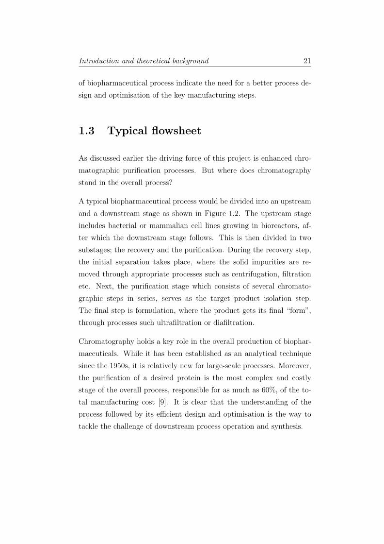
1.3 Typical flowsheet
As discussed earlier the driving force of this project is enhanced chro-
matographic purification processes. But where does chromatography
stand in the overall process?
A typical biopharmaceutical process would be divided into an upstream
and a downstream stage as shown in Figure 1.2. The upstream stage
includes bacterial or mammalian cell lines growing in bioreactors, af-
ter which the downstream stage follows. This is then divided in two
substages; the recovery and the purification. During the recovery step,
the initial separation takes place, where the solid impurities are re-
moved through appropriate processes such as centrifugation, filtration
etc. Next, the purification stage which consists of several chromato-
graphic steps in series, serves as the target product isolation step.
The final step is formulation, where the product gets its final “form”,
through processes such ultrafiltration or diafiltration.
Chromatography holds a key role in the overall production of biophar-
maceuticals. While it has been established as an analytical technique
since the 1950s, it is relatively new for large-scale processes. Moreover,
the purification of a desired protein is the most complex and costly
stage of the overall process, responsible for as much as 60%, of the to-
tal manufacturing cost [9]. It is clear that the understanding of the
process followed by its efficient design and optimisation is the way to
tackle the challenge of downstream process operation and synthesis.

Introduction and theoretical background 22
Bioreaction
Centrifugation / Filtration
Capture chromatography
Intermediate chromatography
Polishing chromatography
Ultrafiltration / Diafiltration
Upstream
Downstream
Recovery
Purification
Formulation
<<
<<
Figure 1.2: Flowsheet of a typical biochemical process
1.4 Chromatography
Ettre [10] defines chromatography as “a physical method of separation
in which the components to be separated are distributed between two
phases, one of which is stationary (stationary phase) while the other
(mobile phase) moves in a definite direction” .
1.4.1 History of chromatography
The first scientific evidence demonstrating chromatographic phenomena
was reported at the end of the 19th century. It was not until 1906, how-
ever, that marked the beginning of the era of column chromatography.
At that time, Mikhail Tswett, a Russian botanist, published his work
on the separation of chloroplast pigments in leaf extracts [11]. Through

Introduction and theoretical background 23
his experiments, Tswett identified that adsorption was the mechanism
responsible for separation. It was then that the potential of chromatog-
raphy, as a means of identifying compounds by properties other than
their colour was realised. Tswett is considered to be “the father of
chromatography”, firstly because he coined the term chromatography,
coming from the combination of two Greek words “χρωµα”, meaning
colour, and “γραφειν”, meaning to write, and secondly because he was
the first one who scientifically described the process [12].
In the 1940s, Martins and Synge proposed liquid-liquid partition chro-
matography using as a chromatographic stationary phase silica gel
loaded with water. Martin suggested the potential use of a gaseous
mobile phase [13] but only published this work a decade later [14]. In
1949, Maclean and Hall introduced the first effective form of thin-layer
chromatography (TLC) that was later on extensively developed and
became an extremely effective separation technique with a wide field of
applications [15].
After James and Martin introduced the idea of a gaseous mobile phase,
gas-liquid chromatography (GLC) was rapidly developed as it was a
simple and inexpensive process. Despite its wide range of application,
GLC had several problems, therefore attention was turned to the de-
velopment of liquid chromatography (LC) [15].
Modern liquid chromatography was introduced in the late 1960s-1970s.
Nowadays, liquid chromatography incorporates special column packings
and fully automated equipment. High performance liquid chromatog-
raphy (HPLC) can now achieve faster and sharper separations [16].
1.4.2 How does chromatography work?
As a process of separation, it aims at converting a mixture into its
different components, usually by passing it through an adsorbent sur-
face [17]. In Figure 1.3, a schematic of the chromatographic process is

Introduction and theoretical background 24
demonstrated. A sample feed is introduced in the inlet and each com-
ponent in the mixture migrates at a different rate along the column.
The components with the lower affinity to the stationary phase will
travel faster, therefore elute first from the column. As shown in Figure
1.3, component 2 has a higher affinity for the stationary phase and is
adsorbed, while the less adsorbed part of the mixture (component 1)
is carried along by the mobile phase, until its elution. Emergence of
the outlet is monitored by a detector and the components are collected
in sequence producing an output signal; a chromatogram. Eventually,
each component leaves the column and passes through the detector.
The time between injection and elution, in which each component is
retained in the column, is the retention time, a characteristic for each
component.
Figure 1.3: Chromatographic separation of a two component mix-ture

Introduction and theoretical background 25
1.5 Types of chromatographic separation
There are many different types of chromatography, classified according
to the nature of the mobile and stationary phases, the scale of opera-
tions and operation modes.
1.5.1 Nature of mobile and stationary phase
There are two main classes of chromatography depending on the na-
ture of the mobile and stationary phases: gas chromatography (GC)
and liquid chromatography (LC). In gas chromatography, the mobile
phase is commonly a gas. The stationary phase can be a solid or liquid
adsorbent distributed over the column’s surface. In liquid chromatog-
raphy, the mobile phase is a liquid and the stationary phase consists
of small particles that are usually porous [18]. In this thesis, the focus
is on liquid column chromatography, mainly used in biopharmaceutical
processes.
1.5.2 Scale of operation
Depending on the scale of operation, liquid chromatography can be di-
vided into ultra scale down, analytical, laboratory scale and process
chromatography as summarised in Table 1.2. In ultra scale down the
volumes are in the µg-range and can be used early in the process devel-
opment. In the analytical scale, the volumes are in the µg-range and
the aim is to identify the components of the sample. The laboratory
scale or preparative chromatography is in the g-scale, used for both
analytical and production purposes depending on the process. Finally,
in the production or process chromatography, the volumes are in the
kg-range and the objective is to purify the target component in order
to manufacture a drug.

Introduction and theoretical background 26
Table 1.2: Definitions of the scale of chromatographic separations
Scale Purpose Product Column dimensionsquantity (l x d), mm
Ultra Scale Down Information for µg 12 x 4process synthesis
Analytical Information for µg 250 x 4.6mixture’s composition
Laboratory Substance isolation g 250-300 x 10-100
Process Preparation of kg 300 x 1000purified material
1.5.3 Modes of operation
There are three modes in which column chromatography can be op-
erated: elution, displacement and frontal, as defined by Tiselius [19].
There are also some intermediate modes of operation such gradient elu-
tion, recycling, simulated moving bed etc. In the following section the
three main modes will be discussed along with some intermediate modes
that are used in process chromatography.
Elution Chromatography
In elution chromatography the sample is introduced into the column,
followed by the mobile phase (see Figure 1.4). The sample components
migrate at different rates, hence elute in a series of peaks. As each
component in the mixture migrates at a different rate along the column,
the mixture separates. The rate of migration of each component of the
mixture depends on interactions between the component and both the
mobile and stationary phases.
Elution chromatography can be carried out under three different con-
ditions depending on the mobile phase composition as shown in Figure
1.5:

Introduction and theoretical background 27
Protein A
Protein B
Elution
Figure 1.4: Elution chromatography
• Isocratic elution: In isocratic elution the mobile composition of
the mobile phase is kept constant throughout the elution process
1.5(a).
• Gradient elution: In gradient elution the composition of the mo-
bile phase is increased gradually during the elution process 1.5(b).
• Step elution: The composition of the mobile phase changes peri-
odically 1.5(c).
The most common mode of operation in process chromatography is the
gradient elution (linearly increased) [18].

Introduction and theoretical background 28
(a) Isocratic elution (b) Gradient elution
(c) Step elution
Figure 1.5: Types of elution chromatography
Displacement Chromatography
In displacement chromatography, the sample mixture is fed into the
column and all the compounds in the mixture must compete for the
immediately available adsorption sites. The displacer (a substance with
high affinity to the stationary phase) first displaces the compound with
the strongest adsorption site (protein A in Figure 1.6). Subsequently,
this component will now become the displacer for the next one. Each
component is displaced progressively by the previous one until they
all pass through the column. This mode of operation is not used in
analytical and preparative scale chromatography. In process scale, it
is rarely used mainly because of the lack of suitable protein displacers
[20].

Introduction and theoretical background 29
Protein A & B
Protein A
Protein B
Displacer
Displacement
Figure 1.6: Displacement chromatography
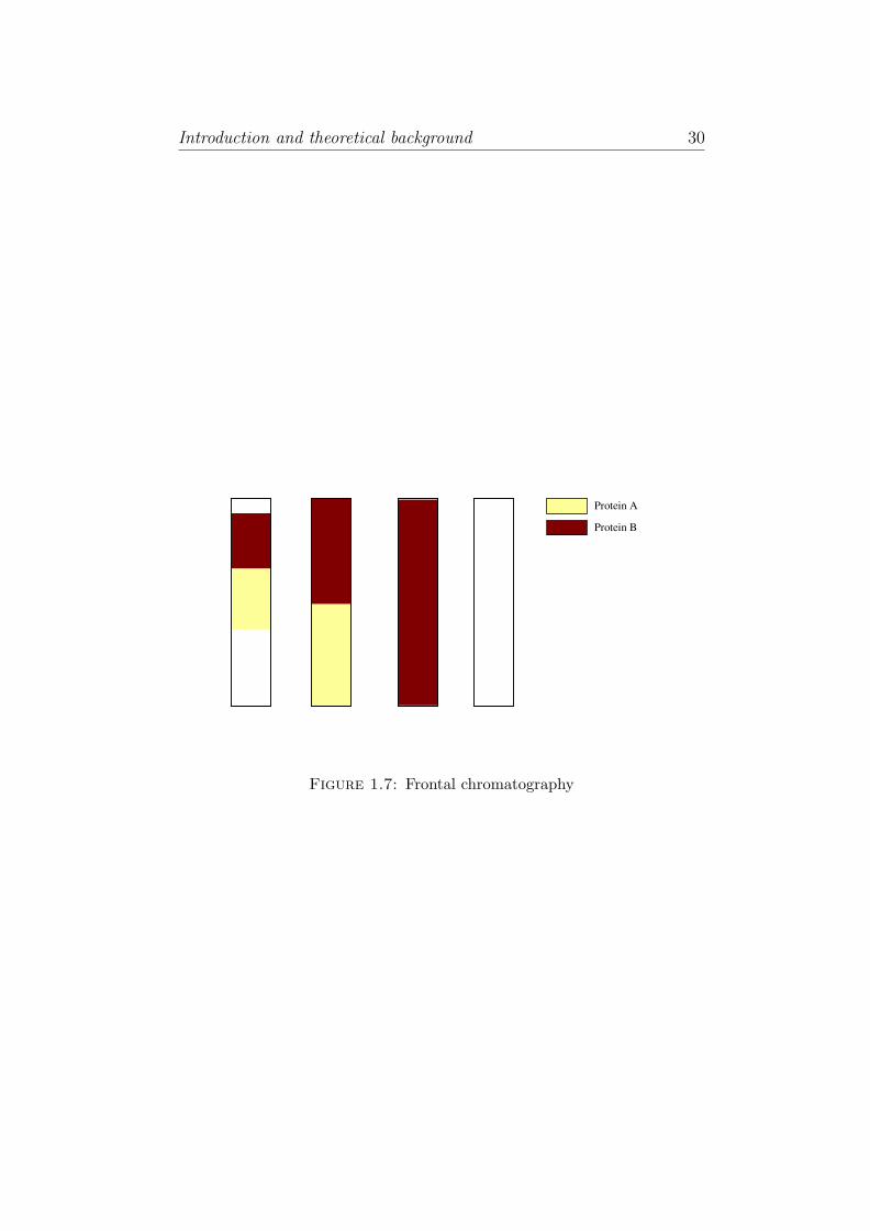
Frontal Chromatography
In this type of chromatography, the sample is fed continuously into the
column. First the mobile phase is collected at the end of the column
and subsequently the components are held with a rate of increasing
affinity to the stationary phase. As shown in Figure 1.7, protein A is
held least strongly in the stationary phase, hence elutes first from the
column, followed by protein B. Frontal analysis is not used for analytical
applications.
1.6 Principles of separation
In this section, the different principles of separation encountered in
chromatographic operations are discussed. Six main categories of such
chromatography are described: ion exchange chromatography (IEX),
hydrophobic interaction chromatography (HIC), reversed phase chro-
matography (RPC), affinity chromatography (AC), size exclusion chro-
matography (SEC) and mixed mode chromatography (MMC). A sum-
mary of the different separation principles is presented in Table 1.3.
Introduction and theoretical background 30
Protein A
Protein B
Frontal
Figure 1.7: Frontal chromatography

Introduction and theoretical background 31
Table
1.3
:Su
mm
ary
ofpr
inci
ples
ofse
para
tion
Typ
eof
chro
mato
gra
phy
Separa
tion
pri
nci
ple
Use
Ion
exch
ange
Surf
ace
char
geR
emov
alof
char
ged
conta
min
ants
Sam
ple
conce
ntr
atio
n
Hydro
phob
icin
tera
ctio
nH
ydro
phob
icit
yR
emov
alof
hydro
phob
icco
nta
min
ants
Sam
ple
conce
ntr
atio
n
Rev
erse
d-p
has
eH
ydro
phob
icit
ySam
ple
conce
ntr
atio
nan
ddes
alti
ng
ofp
epti
des
Rem
oval
ofhydro
phob
icco
nta
min
ants
Sep
arat
ion
ofco
mple
xp
epti
de
sam
ple
s
Affi
nit
yB
iolo
gica
lfu
nct
ion
One
step
puri
fica
tion
ofta
rget
mol
ecule
sfr
omco
mple
xsa
mple
sP
uri
fica
tion
ofta
gged
reco
mbin
ant
pro
tein
sG
roup
separ
atio
ns
Rem
oval
ofsp
ecifi
cco
nta
min
ants
Siz
eex
clusi
onM
olec
ula
rsi
zean
dsh
ape
Sam
ple
condit
ionin
g(d
esal
ting,
buff
erex
chan
ge)
Rem
oval
oflo
wM
ror
hig
hM
rco
nta
min
ants
Sep
arat
ion
ofco
mple
xsa
mple
s
Mix
edm
ode
Dep
ends
onth
ety
pe
Sep
arat
ion
ofen
zym
es,
hum
anse
rum
pro
tein
san
dpla
nt
pro
tein
sV
acci
ne
puri
fica
tion
pro
cess
es

Introduction and theoretical background 32
Ion Exchange Chromatography (IEC): A reversible adsorption
process takes place, in which exchange of ions occurs between the aque-
ous mobile phase and the charged surface of the stationary phase, as
shown in Figure 1.8.
-
-
-
-
-
-
-
--
-
-
+
+
+
+
+
+
+ +
+
+
+
+
+
++
+++ ++
-
+
+
+
+
+
+
+
++
+
+
-
-
-
-
-
-
- -
-
-
-
-
-
--
--- --
+
Figure 1.8: Mechanism of ion exchange chromatography(a) Anion exchange (b) Cation exchange
The stationary phase is usually an insoluble polymeric matrix that is
permeable to ionic solutes. The mechanism responsible for separation is
ion-exchange of solute ions X and mobile phase ions Y with the charged
groups R of the stationary phase [18].
X− +R+Y − = Y − +R+X− (anion exchange) (1.1)
X+ +R−Y + = Y + +R−X+ (cation exchange) (1.2)
The stronger the component ion X interacts with the exchanger ion, the
stronger it is retained in the column. For cation exchange chromatog-
raphy positively charged ions are separated, while for anion exchange
chromatography negatively charged ions are separated. As ion exchange

Introduction and theoretical background 33
chromatography can be carried out with a mobile phase close to phys-
iological conditions, it is a very important technique used for protein
separation.
Hydrophobic Interaction Chromatography (HIC): The interac-
tion between the hydrophobic regions of the solutes’ surface and the
non-polar ligands of the stationary phase is the driving force in this
type of chromatography. As shown in Figure 1.9, the compound with
prominent hydrophobic site binds stronger while the one of low hy-
drophobicity does not bind.
Hydrophobic groups attached to the matrix
High hydrophobicity compound
Medium hydrophobicity compound
Low hydrophobicity compound
Figure 1.9: Mechanism of hydrophobic interaction and reversed-phase chromatography
The basic principle of HIC is similar to that of the reverse phase chro-
matography (RPC), only the conditions are milder, hence it is a tech-
nique appropriate for protein purification. Hydrophobic interaction
chromatography can be very selective. This technique can be used for
the separation of components with similar size and charge, since small
differences in surface hydrophobicities between the solutes can be used
as an efficient means of separation.

Introduction and theoretical background 34
Reverse-phase Chromatography (RPC): Reverse-phase chromatog-
raphy involves a hydrophobic stationary phase and the separation prin-
ciple is similar to the one of HIC as shown in Figure 1.9. The difference
between HIC and RPC is that in RPC, the medium is highly substi-
tuted with hydrocarbon chains. This makes the RPC very hydrophobic,
hence the proteins can adsorb even when diluted in water, while in HIC
the need of salt is necessary in order to achieve adsorption. The adsorp-
tion in RPC is so strong that requires eluents to achieve desorption [21].
These eluents can affect the protein stability, hence this technique is not
preferred for protein purification where biological activity is important.
Size exclusion chromatography (SEC):
In size exclusion chromatography or gel filtration, the bed is packed
with a porous gel which separates the compounds of a mixture depend-
ing on their difference in molecular mass and shape. The larger com-
pounds elute first since they can not enter the pores. Smaller molecules
permeate the pores and move through the column slowly.
High molecular mass compound
Low molecular mass compound
Figure 1.10: Mechanism of size exclusion chromatography

Introduction and theoretical background 35
Affinity Chromatography (AC):
In affinity chromatography, the matrix is coupled with a ligand which
has the ability to bind the target molecule as shown in Figure 1.11.
The adsorption mechanism is the result of molecular recognition. For
example, an enzyme might preferentially bind to ligand sites on the
matrix that mimic the natural substrate of the enzyme. Solutes that
do not have substrate-binding sites that are structurally related to the
matrix ligand sites will be poorly bound, if at all, on to the matrix. The
unbound molecules flow through the column while the components that
bind are subsequently eluted.
Binding site
Molecules with complementary binding sites
Molecules without complementary binding sites
Figure 1.11: Mechanism of affinity chromatography
Mixed Mode Chromatography (MMC):
In this type of chromatography, different separation principles are ap-
plied in order to resolve a mixture to its components. Some exam-
ples of mixed mode chromatography are hydrophobic charge interaction
chromatography (HCIC) and hydroxyapatite chromatography (HC).
In HCIC, adsorption is based on mild hydrophobic interaction and is

Introduction and theoretical background 36
achieved without addition of salts but by reduction of pH. In HC, neg-
atively charged carboxyl groups and positively charged amino groups
of the mobile phase interact with the stationary phase involving posi-
tively charged calcium ions and negatively charged phosphate ions re-
spectively, hence HC can be considered as mixed-mode ion exchange
chromatography. HCIC is usually applied to mixtures where the com-
ponents have very similar isoelectric points and HC is commonly used
for viral removal [22].
1.7 Aims and objectives
Albeit chromatography has been used for the last five decades, more
efficient operation and design remain within the current scope of im-
provement. Chromatography has always been of significant interest for
industry because of its complexity and high capital and operating costs
involved [23]. It still accounts for up to 60 % of the total manufacturing
cost of the final product [24]. Further development of chromatographic
operations represents one of the most significant challenges for the bio-
pharmaceutical industry.
Motivated by the necessity of enhanced chromatographic processes, the
aim of this work was to develop models based on mathematical program-
ming techniques in order to enhance downstream processing.
1.8 Outline of the thesis
The rest of the thesis is divided in five chapters. Chapter 2 discusses the
literature in downstream process operation and synthesis. An overview
of the different methods, models and techniques are analysed.

Introduction and theoretical background 37
Chapter 3 addresses the problem of synthesis of downstream protein
processing that incorporates product losses. The problem is formu-
lated as a mixed integer non-linear programming (MINLP) framework
and integrates the selection of optimum number of chromatographic
techniques along with the timeline when the product is collected.
Chapter 4 describes the development of a mixed integer linear program-
ming (MILP) model for tackling the same problem as that described
in Chapter 3, by modifying the MINLP model through piecewise linear
approximations of the non-linear functions, in order to improve com-
putational efficiency.
An alternative MILP model using discrete recovery levels is introduced
in Chapter 5. The methodology for all the developed models is illus-
trated through their application on three examples containing up to 21
candidate alternative steps and 13 proteins.
In Chapter 6, a model based on first principles was developed in order
to validate the optimisation models described in the previous chapters.
The example used was a four-protein mixture in a purification flowsheet
containing two chromatographic columns.
Finally, Chapter 7 summarises the main contributions of the thesis and
provides suggestions for future work.

Chapter 2
Literature Review
2.1 Drivers for change
Process chromatography has been a prime tool of industry for the last
decades. Its development within the last 20 years resulted into a large
rise of revenues for the major healthcare companies [25]. Although
alternative bioseperation technologies are making their way into the
market, process chromatography will remain a high resolution process
for industry in the years to come [26].
Advances in cell cultures that have resulted in increased titers along
with the strict requirements for purification of today’s therapeutics have
shifted most of the burden to downstream processing [27–29]. As a
result, manufacturers are exploring multiple ways for achieving more
systematic purification processes [30, 31].
This emphasises the need for new tools and strategies that can pro-
vide solutions for the challenges faced in downstream processing design
[32]. This is also encouraged by the Food and Drug Administration
(FDA) [33]. To overcome the bottleneck of downstream processes in a
multiproduct biopharmaceutical facility, different decisions need to be
taken at different levels. The first level of decision is related to design
38
Literature Review 39
and operation, where process alternatives are evaluated and operating
conditions are determined. The second level is related to scheduling
where sequence and timing of the selected unit operations are decided.
Simultaneously describing process conditions, process alternatives and
plant scheduling would be the ideal strategy. Although there have been
efforts for the simultaneous process synthesis, operation and schedul-
ing of a biopharmaceutical process, as it will be described in section
2.4, to date, there are no adequate methodologies for efficient protein
purification process design and synthesis.
This work focuses on the first level of decisions and more specifically
on process synthesis and operating conditions. Below, a brief litera-
ture review on recent work determining both operating conditions and
chromatographic trains will be discussed.
2.2 Operation of chromatographic processes
In traditional methods for operating chromatographic techniques, the
focus has been to deal with each step individually. Investigating the
performance and robustness of a chromatographic column has been a
significant part of research. As discussed in Chapter 1, many different
modes of operation and principles of separation exist, therefore there
was a large spectrum of possibilities to investigate. An overview of
alternative approaches is presented below.
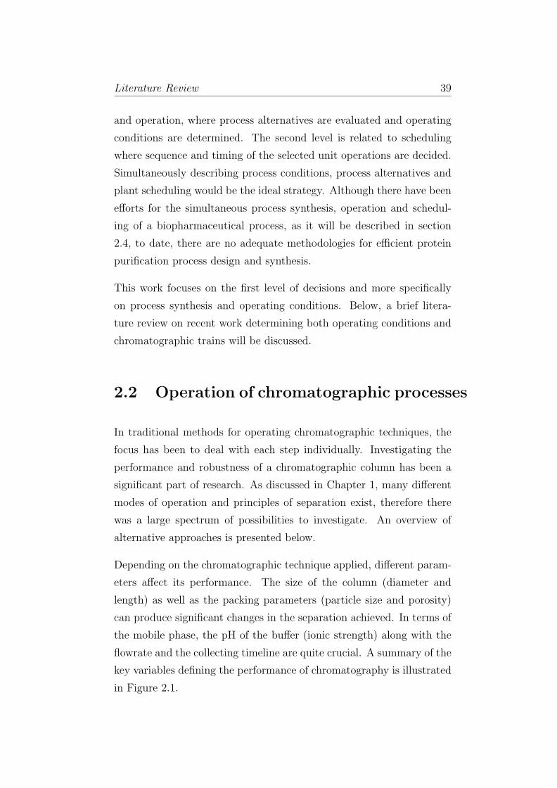
Depending on the chromatographic technique applied, different param-
eters affect its performance. The size of the column (diameter and
length) as well as the packing parameters (particle size and porosity)
can produce significant changes in the separation achieved. In terms of
the mobile phase, the pH of the buffer (ionic strength) along with the
flowrate and the collecting timeline are quite crucial. A summary of the
key variables defining the performance of chromatography is illustrated
in Figure 2.1.

Literature Review 40
Performance
Resin properties Column geometry
Mobile phase
properties
Particle
size
Matrix
porosity
Column
length
Column
diameter
Ionic
strength
Flowrate
Collecting
timeline
Figure 2.1: Key performance parameters
Apart from the parameters mentioned above, depending on the princi-
ple of separation applied, there are some specific key parameters affect-
ing the column performance. For example, in ion exchange chromatog-
raphy some of the key design variables are: the pH and the charge
strength [34]. For hydrophobic interaction chromatography, the polar
solvent and the type of hydrophobic ligand can have a significant im-
pact in the column performance [35]. Since, ion exchange chromatog-
raphy and hydrophobic interaction are two of the most widely used
chromatographic techniques for protein purification in the biopharma-
ceutical industry [36, 37], a great part of the research has focused in
these two techniques.
Different approaches have been used, in order to evaluate the perfor-
mance and robustness of a chromatographic process within a single

Literature Review 41
column. These approaches can be divided into the following cate-
gories: protein structure approaches, mechanistic approaches, graphical
approaches and black box approaches.
2.2.1 Protein structure approaches
In these approaches, the 3-D structure of the protein is taken into ac-
count as well as its orientation when in contact with a a binding sur-
face. Hubbuch and coworkers [38] initially focused on understanding
the binding mechanism between protein and resin and then studied the
effect of ionic strength and mobile phase pH on the binding orientation
of lysozyme in different IEX resins [39].
Later, they used experimental data on adsorption of lysozyme in dif-
ferent ion exchange resins and developed a more detailed model that
proved how significant is the effect of the ligand density in the adso-
prtion behavior of lysozyme [40].
2.2.2 Mechanistic approaches
In mechanistic approaches, the phenomena that take place in the col-
umn are taken into account. Mass transfer through diffusion and con-
vection have been mathematically described by many researchers. Mod-
elling chromatographic processes has been a complex task, largely due
to the complexity of the process itself and the interactions between the
compounds to be separated. Significant research work focused on tack-
ling this challenge. Initially, modelling chromatography has resulted in
improved understanding of the physical phenomena that take place in
the column. Enhanced understanding resulted in the prediction of the
system behaviour and the better design configuration and operation of
the process.
The selection of the appropriate model is an important issue and many
research groups have worked in developing new models and evaluating

Literature Review 42
existing ones. There are several mathematical models based on first
principles that have widely been studied in the literature. The most
common ones are: plate model and rate models (ideal model, equilib-
rium dispersive model, general rate model). These models are discussed
and analysed in detail in Chapter 6.
Many research groups have evaluated different modelling approaches,
applying them to both ion exchange and hydrophobic interaction chro-
matography [41–44]. Although plate model has worked fine in some
cases [45] and has even been used for an industrial practical application
[46], it is still not the preferred one mainly because of the lack of flexi-
bility for complex mixtures where protein interactions have a significant
role.
On the contrary, the rate model takes into account adsorption kinetics
therefore is capable of describing these interactions but is computa-
tionally demanding. Rate models have been extensively used in the
literature [44, 47, 48], with the equilibrium dispersive model being the
common choice, mainly because it provides a good enough description
of the phenomena taking place in the column without a priori require-
ments of many parameters and is relatively easier to implement and
solve computationally than the general rate model.
In most cases, the developed models were used in order to predict the
best operating conditions of a single chromatographic column. This was
achieved by changing some of the crucial parameters such as flowrate
or ionic strength gradient for IEX, followed by some sort of qualitative
or quantitative evaluation of the separation achieved.
Karlsson et al [41], used the general rate model to simulate a three
protein mixture in an ion-exchange chromatography step and investi-
gate the impact of loading time and gradient in the elution. Orellana
et al [48] also used the general rate model to simulate a three protein
mixture in IEX. They were interested in the effect of flowrate and the
initial protein concentration on the retention time.

Literature Review 43
Degerman and coworkers [49], used the general rate model and evalu-
ated the critical process parameters by using the worst case scenario
method where purity was lowest possible for the purification of im-
munoglobulinG through ion exchange chromatography. The worst case
approach was also used by Jakobsson et al [50], where they tried to
evaluate the robustness of an ion exchange chromatography step for a
two-protein mixture.
2.2.3 Graphical approaches
The output of a chromatographic process is a chromatogram. How-
ever, it is not easy to extract the sensitivity of a chromatogram under
different operating conditions [51]. For this reason, several graphical
approaches have been developed by various research groups in order
to describe the reaction of a chromatographic stage when changing the
operating conditions.
Ngiam et al [51] calculated chromatographic performance by using frac-
tionation diagrams to represent recovery trade-offs for a three-component
mixture in size exclusion chromatography.
Multivariate statistical analysis is another graphical approach used by
Tichener-Hooker and co-workers, where a small set of experimental sep-
arations can be enough to investigate a wide range of separation char-
acteristics and variables affecting chromatographic performance [52].
The necessity to look at chromatographic techniques as a whole and pro-
duce an optimal set of operating conditions led Tichener-Hooker and
coworkers [23] to apply some graphical approaches for a three-protein
mixture by three consecutive chromatographic techniques. Later, from
the same group the tie-line method was used to decrease the window
of operation for a three protein mixture through two consecutive chro-
matographic techniques, in order to quantify the trade-offs between
purity and recovery [53].

Literature Review 44
2.2.4 Black-box approaches
In this type of approaches, there is no need to take into account the
physical phenomena that take place in the column. Such typical meth-
ods include partial least squares (PLS), artificial neural networks (ANN)
and support vector regression (SVR). Cramer and his group have done
a lot of research in this field on both IEX and HIC where they used
structural descriptors along with statistical evaluation of experiments
to predict protein retention behaviour [54–56] and HIC [57–59].
A disadvantage of all the methods described above is that the system
configuration is known a priori, hence only the operating conditions are
being evaluated, although the determination of the number of steps is
a major challenge for the biopharmaceutical industry.
2.3 Synthesis of chromatographic processes
A typical biochemical process usually involves several chromatographic
steps so as to achieve a final product according to confined specifica-
tions. However, biopharmaceutical companies usually operate in sub-
optimal conditions and for this reason, many efforts have focused on
developing systematic methods, for the efficient design of process chro-
matography.
Some of the strategies are based on high throughput experimentation,
knowledge-based approaches and algorithmic or optimisation-based tech-
niques as discussed below.
2.3.1 High-throughput experimentation
In this strategy, conventional or high-throughput screening is conducted,
where some of the key design variables are investigated in order to get

Literature Review 45
the optimal values [60, 61]. This requires a large number of measure-
ments, nevertheless there is no guarantee that the final solution will be
the best one. Trial and error methods were quite common even in the
industrial scale [43]. In order to create some rational tools for process
design, researchers started looking for more systematic methodologies
[62].
2.3.2 Heuristics or knowledge-based approaches
First efforts started in the late 80s and employed heuristics (rules of
thumb) in designing purification processes [36, 63–70]. These methods
were based on insights and available knowledge [71]. The aim has always
been to produce a product with the highest possible purity and yield
using the minimal resources (cost). In order to rationalise the method-
ology researchers employed sets of rational rules that would ensure the
required specifications. An example of these rules was presented by
Asenjo and coworkers [69], reproduced below.
• Rule 1: Decide on separation process based on different physico-
chemical properties.
• Rule 2: First remove the impurities in abundance.
• Rule 3: Choose those processes that will exploit the differences
in the physicochemical properties of the product and impurities
in the most efficient manner.
• Rule 4: Use a high-resolution step as early as possible.
• Rule 5: Do the most arduous step last.
Further efforts employed expert knowledge and systematic approaches
to select unit operations in order to synthesise economically favourable
processes, based on the ability of chromatographic techniques to exploit
differences in physicochemical properties of the compounds within the
Literature Review 46
mixture [71–75]. These methods inherently hold the drawback of being
qualitative and cannot guarantee that the proposed solution is the best
due to the size of the design space. Nonetheless they hold the advantage
of reducing the search space to a level where quantitative analysis can
be employed.
2.3.3 Optimisation-based approaches
In recent years, advances in mathematical programming techniques,
solvers and computer power laid the foundation for the use of algorith-
mic and optimisation based techniques.
Early efforts were based on physicochemical properties to screen pu-
rification unit operations together with a mixed-integer non-linear pro-
gramming (MINLP) problem for the final process synthesis [76, 77].
Later on, several authors reported mathematical models based on mixed-
integer linear programming (MILP). In [2, 78], two MILP models were
developed, utilising physicochemical properties of all the components in
the mixture, in order to synthesise the optimal flowsheet for a specified
purity and recovery.
In addition, these have been combined with the physicochemical prop-
erties of amino acids to predict the behaviour and design of peptide-
fusion tags that alter the purification of proteins [79–82]. Such optimi-
sation methods can be very powerful when combined with systematic
approaches to obtain the necessary input parameters, as they signifi-
cantly reduce the design search space [32, 83].
Under the assumption of complete product recovery, several optimisa-
tion models have been developed [78, 80]. However, the flexibility of also
selecting the times of product collection (peak cut-points) provides the
opportunity to capture the trade-offs between product quality (purity)
and quantity. Previous work partially tackled this challenge allowing
discrete percentage levels of product collection [84, 85].

Literature Review 47
2.4 Simultaneous process operation and
synthesis
One important challenge in chromatography is to simultaneously de-
scribe process conditions, process alternatives and plant scheduling.
Samsatli et al [86–88] proposed a two-stage approach, where the first
stage was related to the conditions of the unit operations of a multi-
product plant and the second to the scheduling of the process. The
only structural decisions made in the first stage are related to the num-
ber of fermentors working in parallel while the purification process was
predetermined.
Later, Asenjo and coworkers [89–91] tried tackling the same problem
for a plant aiming to produce four recombinant proteins including hu-
man insulin, hepatitis B vaccine, chymosin and cryophilic protease. In
this approach, time and size factors were used to evaluate the different
design configurations. Decisions involved the number of fermentors and
chromatographic columns working in parallel as well as storage tanks.
More recently, Asenjo and coworkers [92] proposed a methodology where
a two stage approach was used; in the first stage the sequence of chro-
matographic steps is determined and then the operating conditions
(flowrate, ionic strength gradient) are optimised.
2.5 Summary
As seen in the pages above, chromatography has been and still remains a
focus of many researchers around the world. Running chromatographic
steps in the best possible way in order to achieve optimal separation
is a challenge to be tackled. Different approaches were used in order
to achieve the same target; optimal separation. For defining the oper-
ating conditions, the approaches vary from detailed and analytical to
black-box methods. For chromatographic process synthesis, methods

Literature Review 48
were proposed starting from experience and rules of thumb to algorith-
mic and optimisation-based approaches. In this work, we will focus on
optimisation-based methods in order to tackle the challenge of chro-
matographic synthesis and operation.
This work extends a work done by Pinto and coworkers [78], where chro-
matographic trains were synthesised with the assumption of complete
recovery of the product. This work removes the assumption of com-
plete recovery and apart from process synthesis, it also encompasses on
selecting the timeline at which the product is collected, hence this work
essentially incorporates simultaneous process operation and synthesis.
Chapter 3
An MINLP formulation for
purification process synthesis
In this chapter, a novel approach based on mathematical programming
is proposed and a mathematical model for the design of protein pu-
rification processes is presented, along with the fundamental basics of
our model and the solution approach utilised for the specific chromato-
graphic separation problem.
3.1 Introduction
As mentioned in Chapter 1 enhanced downstream process synthesis
holds a key in reducing the manufacturing cost. To achieve that there
are a few suggested strategies such as decreasing the number of steps,
avoiding complex steps and reducing raw material costs. As shown in
[93], many companies adopt molecule specific approaches based on a
particular impurity challenge and can select from a set of candidate
chromatographic steps. Many criteria have to be met for cost effective-
ness, while always meeting stringent purity specifications. Particularly
challenging in this context is the optimum selection of a process se-
quence from the available chromatographic steps.
49

An MINLP formulation for purification process synthesis 50
3.2 Problem statement
The overall problem for the synthesis of the purification processing can
be stated as follows.
Given:
• a mixture of proteins (p: 1,...,P) with known physicochemical
properties (charge and hydrophobicity);
• a set of available chromatographic techniques (i: 1,...,I), each
performing a separation by exploiting a specific physicochemical
property;
• specifications for the desired protein (dp) in terms of minimum
purity and recovery levels.
Determine:
• the flowsheet of the purification process
• operating starting and finishing cut-points (xsi,dp, xfi,dp)
So as to optimise the overall number of chromatographic steps taking
into account product losses.
The model is based solely on the approximation of the chromatographic
peaks by isosceles triangles and uses as inputs the physicochemical prop-
erties of the proteins in the complex mixture as shown in [2], [78].
The main features and basis of the chromatographic operations are ex-
plained in the following section.
An MINLP formulation for purification process synthesis 51
3.3 Basis for the chromatographic separa-
tion model
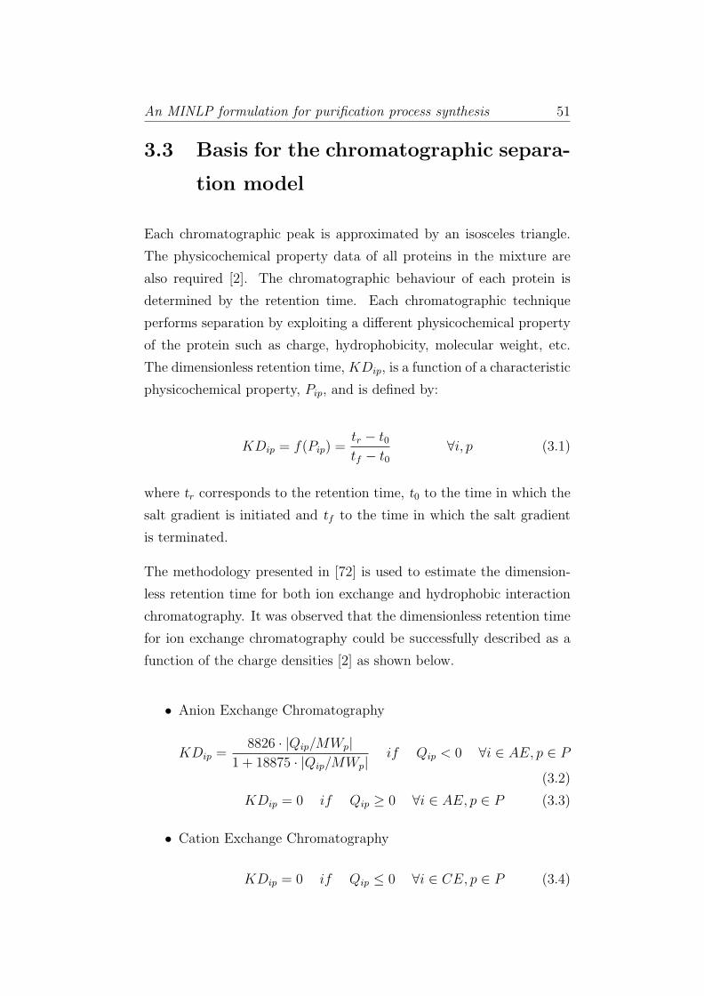
Each chromatographic peak is approximated by an isosceles triangle.
The physicochemical property data of all proteins in the mixture are
also required [2]. The chromatographic behaviour of each protein is
determined by the retention time. Each chromatographic technique
performs separation by exploiting a different physicochemical property
of the protein such as charge, hydrophobicity, molecular weight, etc.
The dimensionless retention time, KDip, is a function of a characteristic
physicochemical property, Pip, and is defined by:
KDip = f(Pip) =tr − t0tf − t0
∀i, p (3.1)
where tr corresponds to the retention time, t0 to the time in which the
salt gradient is initiated and tf to the time in which the salt gradient
is terminated.
The methodology presented in [72] is used to estimate the dimension-
less retention time for both ion exchange and hydrophobic interaction
chromatography. It was observed that the dimensionless retention time
for ion exchange chromatography could be successfully described as a
function of the charge densities [2] as shown below.
• Anion Exchange Chromatography
KDip =8826 · |Qip/MWp|
1 + 18875 · |Qip/MWp|if Qip < 0 ∀i ∈ AE, p ∈ P
(3.2)
KDip = 0 if Qip ≥ 0 ∀i ∈ AE, p ∈ P (3.3)
• Cation Exchange Chromatography
KDip = 0 if Qip ≤ 0 ∀i ∈ CE, p ∈ P (3.4)

An MINLP formulation for purification process synthesis 52
KDip =7424 · |Qip/MWp|
1 + 20231 · |Qip/MWp|if Qip > 0 ∀i ∈ CE, p ∈ P
(3.5)
For hydrophobic interaction chromatography, the dimensionless reten-
tion time was given through a quadratic function of hydrophobicity
[94]:
KDip = −12.14 ·H2p + 12.07 ·Hp − 1.74 ∀i ∈ HI, p ∈ P (3.6)
Concentration factors, CFip, indicate the efficiency of each chromato-
graphic technique and is a function of the deviation factor, DFip, the
peak width, σi, which will be explained below. CFip for the various
chromatographic steps are calculated based on the distance between the
chromatographic peaks of the desired product and that of the contam-
inant [2]. Deviation factors, DFip, are defined as the distance between
two peaks (see Figure 3.1), one of them being that of the target protein.
dp
σι
DFιp
p2
Figure 3.1: Graphical representation of deviation factor DFip
DFip = KDip −KDi,dp ∀i, p (3.7)

An MINLP formulation for purification process synthesis 53
As mentioned before, product losses along the purification process are
possible, thus the assumption of 100 % recovery of the product is re-
moved. In order to achieve that, starting xsi,dp and finishing xfi,dp
cut-points are applied. A graphical explanation of how the cut-points
behave depending on the recovery is presented in Figure 3.2.
time
p4 dp p2 p1p3
(a) 100%, recovery of the target protein
time
p4 dp p2 p1p3
(b) <100%, recovery of the target protein
Figure 3.2: Graphical explanation of cut-points

An MINLP formulation for purification process synthesis 54
In Figure 3.2(a), the cut points are located at the borders of the peak
width, while in Figure 3.2(b), the cut-points can be located across the
peak width line depending on the required recovery.
A brief breakdown of the different cases that may arise depending on
the position of these cut-points is described below. In Figure 3.3, the
triangles refer to the target protein and the shaded areas represent the
remaining amount of the target protein within the mixture after the
chromatographic technique has been applied.
(c) (b) (a)
xfi,dp
xsi,dp σι
xfi,dp
xsi,dp σι
xfi,dp
xsi,dp σι
Figure 3.3: Representation of chromatographic peaks for the tar-get protein
The mathematical expressions presented below represent the three cases
presented in Figure 3.3. The chromatograms are approximated by
isosceles triangles assuming constant shapes. Furthermore, the peak
width has been averaged for each chromatographic technique. The peak
width parameter σi only depends on the type of chromatographic op-
eration and was calculated by averaging over several proteins. For ion
exchange, the value for the peak width is σi=0.15 and for hydrophobic
interaction σi=0.22 [2]. Note that both KDip and σi are both dimen-
sionless or have units of time.

An MINLP formulation for purification process synthesis 55
• xsi,dp, xfi,dp < σi
2
CFi,dp =2 ·(xf 2
i,dp − xs2i,dp
)σ2i
(3.8)
• xsi,dp < σi
2, xfi,dp >
σi
2
CFi,dp = 1− 2 · [(xsi,dp)2 + (σi − xfi,dp)2]
σ2i
(3.9)
• xsi,dp, xfi,dp > σi
2
CFi,dp =2 · [(σi − xsi,dp)2 − (σi − xfi,dp)2]
σ2i
(3.10)
It is important to note that three different cases may arise depending on
the relative positions of the cut-points. In the first case, Figure (3.3a)
both cut-points are applied before the chromatogram has reached its
peak and the other extreme case Figure (3.3c) is valid when both cut-
points are applied after the chromatogram has reached its peak. Finally,
the remaining case shown in Figure (3.3b) is when the starting point
is applied before the chromatogram reaches its peak and the finishing
point is applied after the chromatogram reaches its peak.
For the contaminants, the concentration factor is calculated similarly,
but in this case the concentration factor is also a function of the devi-
ation factor. Many different cases may arise depending on the relative
positions of the triangles and the cut-points as well.
Below, we can see a graphical representation of how the different chro-
matograms can be allocated depending on their peak distance. Re-
tention time data available in [2] were used to create the actual chro-
matograms. In Figure 3.4, we can see a visual representation of how
the different proteins elute in different times and how this results in a
typical separation problem. In all figures, the solid line triangle refers
to the target protein and the rest are considered as contaminants. As

An MINLP formulation for purification process synthesis 56
shown, in some cases, peaks of target protein and contaminants can al-
most completely overlap (difficult to separate) Figures (3.4(a), 3.4(f))
or in other cases the two peaks are far from each other (easy to separate)
Figures (3.4(c), 3.4(d)).
3.4 Mathematical model
The mathematical model for the optimisation of the selection of the
chromatographic steps for the purification of proteins is described next.
Objective Function
An objective function that selects the minimum number of chromato-
graphic steps is defined as follows:
Minimise S =∑i
Ei (3.11)
where Ei is a binary variable, activated when a chromatographic tech-
nique i is selected.
Target Protein Constraints
This set of constraints determines the concentration factors for the tar-
get protein. Binary variables, zsip and zfip, are introduced for starting
and finishing cut-points, respectively. In Figure 3.5, a graphical repre-
sentation of how these variables are activated is presented. Each binary
variable indicates whether the relevant cut-point is located before or af-
ter the chromatogram peak.

An MINLP formulation for purification process synthesis 57
−0.1 −0.05 0 0.05 0.1 0.15 0.2 0.250
0.1
0.2
0.3
0.4
0.5
0.6
0.7dpp2p3p4
(a)
−0.1 −0.05 0 0.05 0.1 0.15 0.2 0.25 0.3 0.350
0.1
0.2
0.3
0.4
0.5
0.6
0.7dpp2p3p4
(b)
−0.1 −0.05 0 0.05 0.1 0.15 0.2 0.25 0.3 0.350
0.1
0.2
0.3
0.4
0.5
0.6
0.7dpp2p3p4
(c)
−0.1 −0.05 0 0.05 0.1 0.15 0.2 0.25 0.3 0.350
0.1
0.2
0.3
0.4
0.5
0.6
0.7dpp2p3p4
(d)
−0.05 0 0.05 0.1 0.15 0.2 0.25 0.30
0.1
0.2
0.3
0.4
0.5
0.6
0.7dpp2p3p4
(e)
0.25 0.3 0.35 0.4 0.45 0.5 0.55 0.6 0.65 0.7 0.750
0.1
0.2
0.3
0.4
0.5
0.6
0.7dpp2p3p4
(f)
Figure 3.4: Typical protein elution problem using data from [2]

An MINLP formulation for purification process synthesis 58
Figure 3.5: Representation of binary variables for the target pro-tein indicated by Equation 3.12
Depending on the values of these binary variables, Equation 3.12 can
cover all possible cases that were demonstrated in Figure 3.3.
CFip = 2 · (xfip)2
σ2i
· (1− zfip) +
[1− 2 · (σi − xfip)2
σ2i
]· zfip
−2 · (xsip)2
σ2i
·(1−zsip)−[1− 2 · (σi − xsip)2
σ2i
]·zsip ∀i, p = dp
(3.12)
Equations 3.13 and 3.14 determine the position within the target pro-
tein’s range for both xsip and xfip. If the cut-point is after the chro-
matogram’s peak (> σi/2), the corresponding binary variable is equal
to one otherwise (< σi/2) is forced to zero.
σi2· zsip ≤ xsip ≤
σi2
+M · zsip ∀i, p = dp (3.13)
σi2· zfip ≤ xfip ≤
σi2
+M · zfip ∀i, p = dp (3.14)
Finally, Constraint 3.15 is a logical constraint that indicates that the
starting cut-point, xsip, should always be before the finishing cut-point,
xfip.
xsip ≤ xfip ∀i, p = dp (3.15)

An MINLP formulation for purification process synthesis 59
Contaminant Protein Constraints
Similarly to the target protein, a set of constraints also applies for
determining concentration factors, CFip, for all contaminants in the
mixture.
All possible cases that may arise depending on the relative position of
the triangles can be calculated by using shifted starting and finishing
cut-points as shown in Equations 3.16 and 3.17. For the shifted cut-
points, the concentration factors of the contaminants CFip also depend
on the deviation factors DFip.
xsip = xsi,dp −DFip ∀i, p 6= dp (3.16)
xfip = xfi,dp −DFip ∀i, p 6= dp (3.17)
If the shifted cut-point is after the chromatogram’s peak (> σi/2), the
corresponding binary variable zsip or zfip is equal to one otherwise
(< σi/2) is forced to zero by constraints 3.18 and 3.19.
σi2−M · (1− zsip) ≤ xsip ≤
σi2
+M · zsip ∀i, p 6= dp (3.18)
σi2−M · (1− zfip) ≤ xfip ≤
σi2
+M · zfip ∀i, p 6= dp (3.19)
Correction variables ∆sip, ∆fip, ∆sip, ∆fip defined in Equations 3.20
- 3.23, along with additional binary variables ysip, yfip, wsip, wfip are
introduced for the shifted starting and finishing cut-points, xsip and
xfip, respectively. These variables are introduced as in many cases the
shifted cut-points are outside the contaminant’s peak width.
∆sip ≡ max (xsip, 0) ∀i, p 6= dp (3.20)
∆fip ≡ max (xfip, 0) ∀i, p 6= dp (3.21)
∆sip ≡ min (xsip, σi) ∀i, p 6= dp (3.22)
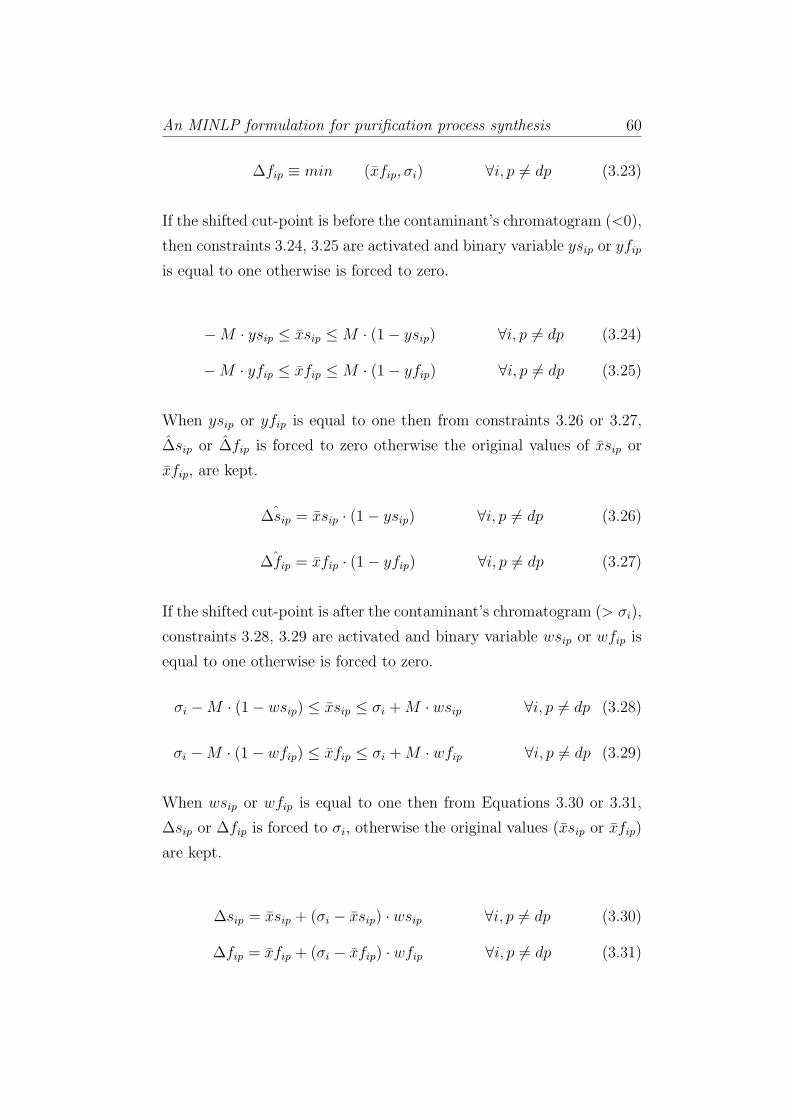
An MINLP formulation for purification process synthesis 60
∆fip ≡ min (xfip, σi) ∀i, p 6= dp (3.23)
If the shifted cut-point is before the contaminant’s chromatogram (<0),
then constraints 3.24, 3.25 are activated and binary variable ysip or yfip
is equal to one otherwise is forced to zero.
−M · ysip ≤ xsip ≤M · (1− ysip) ∀i, p 6= dp (3.24)
−M · yfip ≤ xfip ≤M · (1− yfip) ∀i, p 6= dp (3.25)
When ysip or yfip is equal to one then from constraints 3.26 or 3.27,
∆sip or ∆fip is forced to zero otherwise the original values of xsip or
xfip, are kept.
ˆ∆sip = xsip · (1− ysip) ∀i, p 6= dp (3.26)
ˆ∆fip = xfip · (1− yfip) ∀i, p 6= dp (3.27)
If the shifted cut-point is after the contaminant’s chromatogram (> σi),
constraints 3.28, 3.29 are activated and binary variable wsip or wfip is
equal to one otherwise is forced to zero.
σi −M · (1− wsip) ≤ xsip ≤ σi +M · wsip ∀i, p 6= dp (3.28)
σi −M · (1− wfip) ≤ xfip ≤ σi +M · wfip ∀i, p 6= dp (3.29)
When wsip or wfip is equal to one then from Equations 3.30 or 3.31,
∆sip or ∆fip is forced to σi, otherwise the original values (xsip or xfip)
are kept.
∆sip = xsip + (σi − xsip) · wsip ∀i, p 6= dp (3.30)
∆fip = xfip + (σi − xfip) · wfip ∀i, p 6= dp (3.31)

An MINLP formulation for purification process synthesis 61
In Equation 3.32, the concentration factor for each contaminant is cal-
culated by:
CFip = 2 · (∆fip)2
σ2i
· (1− zfip) +
[1− 2 · (σi −∆fip)
2
σ2i
]· zfip
−2· (∆sip)2
σ2i
·(1−zsip)−[1− 2 · (σi −∆sip)
2
σ2i
]·zsip ∀i, p 6= dp
(3.32)
A graphical representation of how the new binary variables are activated
is shown in Figure 3.6.
Figure 3.6: Representation of binary variables for the contami-nants
Process Synthesis Constraints
The following set of constraints enforces the mass of each protein, mip,
in the mixture t be reduced when the chromatographic technique i has
been selected [2]. Constraint 3.33 indicates the mass of each protein
after the first chromatographic step has been applied, where mop is the
initial mass of each protein. If chromatographic step i is selected (Ei=1
)then the mass of all the proteins in the mixture is forced to be reduced,
otherwise it remains the same. Constraints 3.34 - 3.37 are active for all
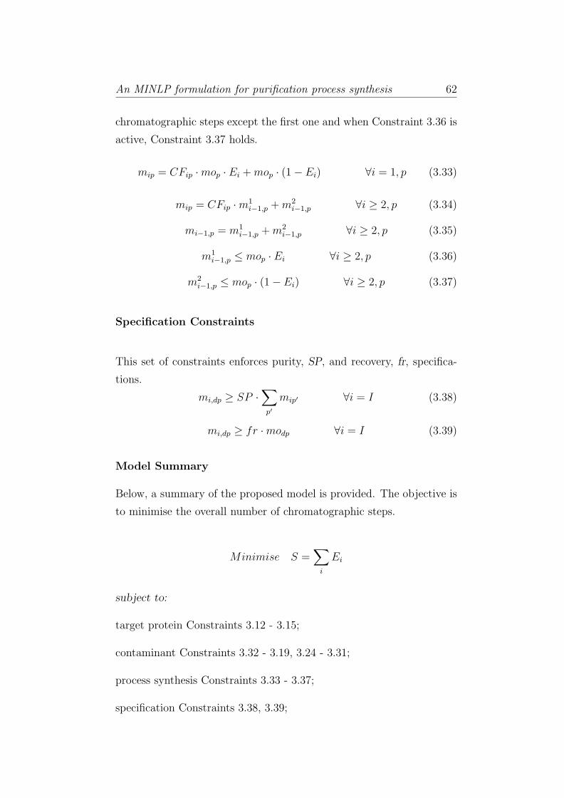
An MINLP formulation for purification process synthesis 62
chromatographic steps except the first one and when Constraint 3.36 is
active, Constraint 3.37 holds.
mip = CFip ·mop · Ei +mop · (1− Ei) ∀i = 1, p (3.33)
mip = CFip ·m1i−1,p +m2
i−1,p ∀i ≥ 2, p (3.34)
mi−1,p = m1i−1,p +m2
i−1,p ∀i ≥ 2, p (3.35)
m1i−1,p ≤ mop · Ei ∀i ≥ 2, p (3.36)
m2i−1,p ≤ mop · (1− Ei) ∀i ≥ 2, p (3.37)
Specification Constraints
This set of constraints enforces purity, SP, and recovery, fr, specifica-
tions.
mi,dp ≥ SP ·∑p′
mip′ ∀i = I (3.38)
mi,dp ≥ fr ·modp ∀i = I (3.39)
Model Summary
Below, a summary of the proposed model is provided. The objective is
to minimise the overall number of chromatographic steps.
Minimise S =∑i
Ei
subject to:
target protein Constraints 3.12 - 3.15;
contaminant Constraints 3.32 - 3.19, 3.24 - 3.31;
process synthesis Constraints 3.33 - 3.37;
specification Constraints 3.38, 3.39;

An MINLP formulation for purification process synthesis 63
domain Constraints: Ei, zsip, zfip, wsip, wfip, ysip, yfip ∈ {0, 1}mip, m
1ip, m
2ip ≥ 0 ∀i, p
3.5 Solution approach
The overall problem is formulated as mixed integer non-linear program-
ming (MINLP) model. The resulting optimisation model is non-convex
and the nonlinearities arise in:
• Equations 3.12 and 3.32, for the calculation of the concentration
factors for both the target protein and the contaminants,
• Equations 3.26 - 3.27 and 3.30 - 3.31 for the estimation of the
correction variables,
• Equations 3.33 - 3.34 for the calculation of the mass of all the
proteins in in the mixture.
Trying to solve the monolithic MINLP resulted in many of the cases in
no solution or into very large CPU times, therefore a two-stage solution
is proposed to identify the optimal flowsheet of the purification process.
Stage 1: Solve screening MILP [78] that does not take into account
product losses, to determine candidate chromatographic steps.
Stage 2: Solve proposed MINLP with losses over the reduced set of
alternatives determined by stage 1.
Note that the screening MILP model is used over the full set of candi-
date chromatographic steps. Its result is a reduced set of candidates,
but not the minimum number of chromatographic steps to achieve prod-
uct specifications. The minimum number of chromatographic steps is
only determined after stage 2 of the solution procedure, where product
losses are taken into account.

An MINLP formulation for purification process synthesis 64
3.6 Results and discussion
The methodology was tested with three examples modelled in GAMS
22.8 [95]. Solutions were obtained using different MINLP solvers on a
Dell Desktop Core Duo 3.25 GB RAM 3.16z,GHz machine.
3.6.1 Example 1
This first example is based on experimental data taken from [2] in-
volving serum from bovine albumin which is the desired product (dp),
ovalbumin (p2), soybean trypsin inhibitor (p3) and thaumatin (p4). The
physicochemical properties as well as the initial protein concentration
of the mixture are given in Table 3.1. In summary, there are 11 candi-
date chromatographic steps: anion exchange chromatography (AE) at
pH4, AE at pH5, AE at pH6, AE at pH7, AE at pH8, cation exchange
chromatography (CE) at pH4, CE at pH5, CE at pH6, CE at pH7,
CE at pH8 and hydrophobic interaction (HI). In Tables A.1 and A.2 in
Appendix A, the calculated dimensionless retention times, KDip and
deviation factors, DFip are presented.
Table 3.1: Physicochemical properties of protein mixture in ex-ample 1
Qip (C/molecule) ×10−17
Protein mop MW p Hp pH4 pH5 pH6 pH7 pH8(mg/ml) (Da)
dp 2 67000 0.86 1.03 -0.14 -1.16 -1.68 -2.05p1 2 43800 0.54 1.40 -0.76 -1.65 -2.20 -2.36p2 2 24500 0.90 1.22 -0.76 -1.54 -2.17 -2.13p3 2 22200 0.89 1.94 1.90 1.98 -1.87 0.91
Initially, the screening MILP was solved for 98 % purity and no losses,
resulting in a reduced set of 3 candidates (AE7, AE8, HI). Then, the
MINLP model was solved for both purity and recovery set to 98 %. The
optimal solution, shown in Figure 3.7, achieves a purity of 98.1 % and

An MINLP formulation for purification process synthesis 65
1st Step
P
R
O
D
U
C
T
0.250 0.657 0.981A E
pH 7.0
2nd Step
H IProtein
Mixture1 0.997 0.980
xs= 0.006
xf= 0.149
xs= 0
xf= 0.2
Figure 3.7: Optimal flowsheet for purification of protein mixturein example 1
98 % recovery, involving two chromatographic steps: AE at pH7 and
HI. In all flowsheets, the number above the arrow refers to purity and
the one below to recovery.
3.6.2 Example 2
This example utilises data available in [2]. The mixture includes target
protein β − 1, 3 glucanase from Bacillus Subtilis and 8 contaminants.
Physicochemical properties along with initial concentrations of the pro-
tein mixture are available in Table 3.2. Overall, we have 21 candidate
chromatographic steps. Besides the ones presented in example 1, we
have additional steps: anion exchange chromatography (AE) at pH4.5,
AE at pH5.5, AE at pH6.5, AE at pH7.5, AE at pH8.5, cation exchange
chromatography (CE) at pH4, CE at pH5, CE at pH6.5, CE at pH7.5,
CE at pH8.5. In Tables A.3 and A.4 in Appendix A, the calculated
dimensionless retention times, KDip, and deviation factors, DFip, are
given.

An MINLP formulation for purification process synthesis 66
Table
3.2
:P
hysi
coch
emic
alpr
oper
ties
ofpr
otei
nm
ixtu
rein
exam
ple
2
Qip
(C/m
olec
ule
)×
10−
17
Pro
tein
mop
MW
pHp
pH
4pH
4.5
pH
5pH
5.5
pH
6pH
6.5
pH
7pH
7.5
pH
8pH
8.5
(mg/
ml)
(Da)
dp
0.62
3100
00
1.46
0.09
-0.6
2-0
.66
-1.0
2-1
.82
-2.3
3-2
.52
-2.5
2-3
.51
p1
0.42
6250
00
1.46
0.09
-1.0
6-0
.98
1.17
-1.7
1-2
.79
-3.5
2-3
.32
-3.3
2p2
0.25
4060
00
1.46
0.09
-0.5
5-0
.22
-0.2
2-0
.26
-0.7
3-1
.26
-1.8
2-3
.51
p3
0.25
6960
00
1.46
0.09
-0.5
5-0
.22
-0.2
2-0
.26
-0.7
3-1
.26
-1.8
2-3
.51
p4
0.09
4060
00
1.46
3.14
1.46
0.28
-0.4
7-0
.89
-1.0
6-1
.08
-1.0
4-1
.01
p5
0.09
6960
00
1.46
3.14
1.46
0.28
-0.4
7-0
.89
-1.0
6-1
.08
-1.0
4-1
.01
p6
2.74
4100
01.
51.
460.
930.
26-0
.35
-0.8
7-1
.31
-1.6
5-1
.9-2
.04
-2.0
6p7
2.74
3290
01.
51.
460.
090
-1.7
-2.7
-2.9
-3.5
1-3
.51
-3.5
1-3
.51
p8
0.25
3550
00.
21.
460.
09-0
.55
-0.2
2-0
.22
-0.2
6-1
.26
-1.8
2-1
.82
-3.5
1
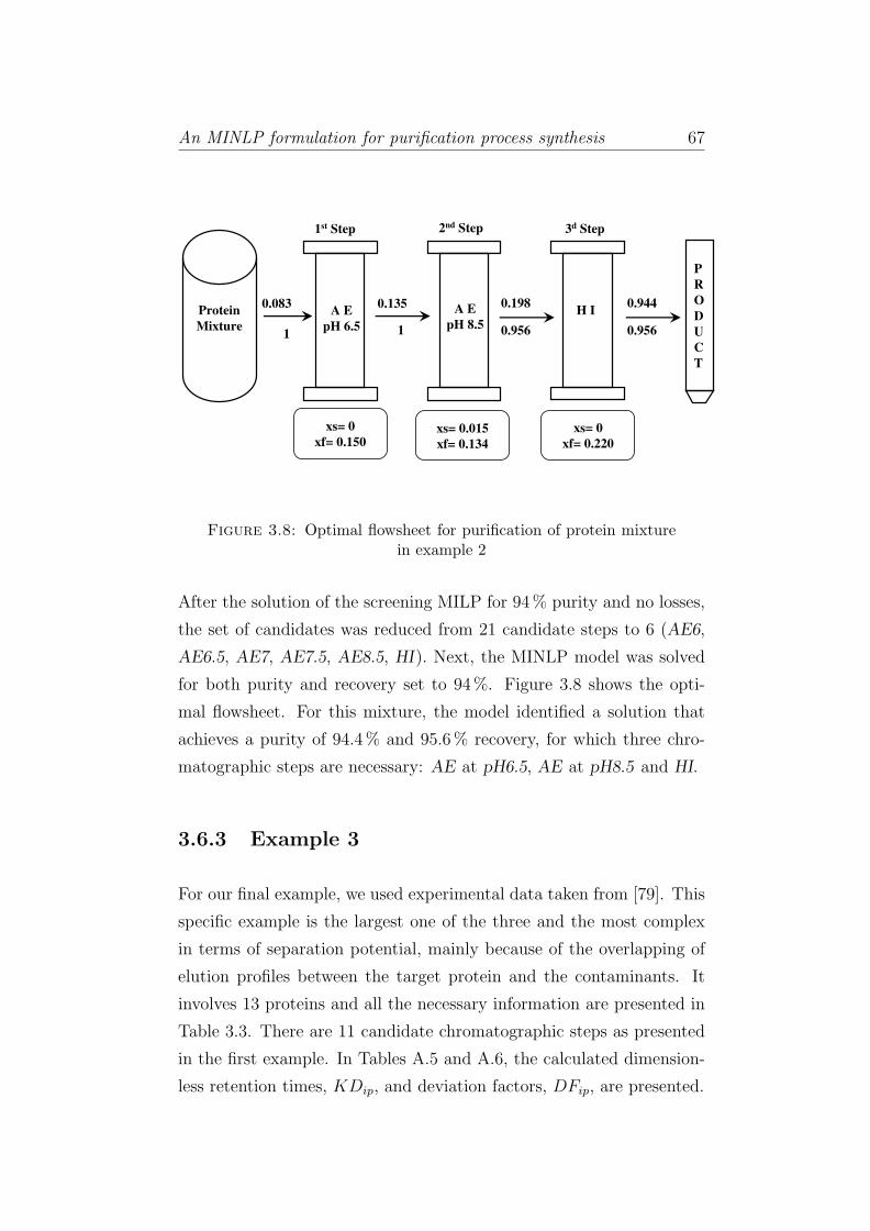
An MINLP formulation for purification process synthesis 67
P
R
O
D
U
C
T
0.083 0.135 0.198A E
pH 6.5
3d Step
H IProtein
Mixture1 1 0.956
xs= 0
xf= 0.150
1st Step 2nd Step
A E
pH 8.5
0.944
0.956
xs= 0
xf= 0.220
xs= 0.015
xf= 0.134
Figure 3.8: Optimal flowsheet for purification of protein mixturein example 2
After the solution of the screening MILP for 94 % purity and no losses,
the set of candidates was reduced from 21 candidate steps to 6 (AE6,
AE6.5, AE7, AE7.5, AE8.5, HI). Next, the MINLP model was solved
for both purity and recovery set to 94 %. Figure 3.8 shows the opti-
mal flowsheet. For this mixture, the model identified a solution that
achieves a purity of 94.4 % and 95.6 % recovery, for which three chro-
matographic steps are necessary: AE at pH6.5, AE at pH8.5 and HI.
3.6.3 Example 3
For our final example, we used experimental data taken from [79]. This
specific example is the largest one of the three and the most complex
in terms of separation potential, mainly because of the overlapping of
elution profiles between the target protein and the contaminants. It
involves 13 proteins and all the necessary information are presented in
Table 3.3. There are 11 candidate chromatographic steps as presented
in the first example. In Tables A.5 and A.6, the calculated dimension-
less retention times, KDip, and deviation factors, DFip, are presented.

An MINLP formulation for purification process synthesis 68
Table 3.3: Physicochemical properties of protein mixture in ex-ample 3
Qip (C/molecule) ×10−17
Protein mop MW p Hp pH4 pH5 pH6 pH7 pH8(mg/ml) (Da)
dp 2 77000 0.28 2.04 1.06 -0.37 -0.81 -1.13p1 2 22000 0.27 1.60 1.57 1.56 1.55 0.75p2 2 23600 0.31 2.15 1.46 1.17 0.78 0.38p3 2 13500 0.23 1.83 0.65 0.26 -0.20 -0.33p4 2 43800 0.28 1.16 -0.63 -1.36 -1.82 -1.95p5 2 15900 0.27 2.89 2.81 2.8 2.64 2.07p6 2 14400 0.32 -0.46 -0.47 -0.63 -1.21 -1.25p7 2 17500 0.21 0.45 -0.62 -0.79 -1.26 -1.7p8 2 50000 0.27 -0.12 -0.32 -0.76 -0.91 -1.04p9 2 12100 0.18 1.46 0.62 -1.02 -1.33 -1.52p10 2 25500 0.30 1.01 -0.63 -1.27 -1.59 -1.76p11 2 26000 0.28 2.96 1.26 0.92 0.54 0.01p12 2 19900 0.25 0.93 0.33 -0.12 -0.34 -0.5
The screening MILP was solved for 93 % purity and no losses, resulting
to a reduced set of 5 candidates (AE6, AE7, CE4, CE5, HI). Then the
MINLP model was solved for a purity of 93 % and a recovery of 90 %.
The optimal solution is presented in Figure 3.9. Three chromatographic
steps are required: AE at pH7, CE at pH4 and HI to achieve a purity
of 93 % and 90 % recovery.
Table 3.4 presents computational statistics for the three examples stud-
ied using the proposed MINLP model and applying the two-stage solu-
tion approach described earlier.
Table 3.4: Summary of Computational Statistics
Example Constraints Discrete/Continuous CPU timeVariables (s)
1 237 63/101 3.12 1188 306/499 2773 1454 375/605 505

An MINLP formulation for purification process synthesis 69
P
R
O
D
U
C
T
0.08 0.213 0.605A E
pH 7.0
3d Step
H IProtein
Mixture1 0.965 0.943
xs= 0.015
xf= 0.137
1st Step 2nd Step
C E
pH 4.0
0.93
0.90
xs= 0.008
xf= 0.188
xs= 0.011
xf= 0.139
Figure 3.9: Optimal flowsheet for purification of protein mixturein example 3
3.6.4 Comparative results
Several MINLP solvers were tested for all three examples. Default
settings were used for all solvers tested. As presented in Table 3.5,
BARON appeared to be the most appropriate solver for the proposed
MINLP model. Although LindoGlobal obtained a solution for all three
examples, the CPU time was significantly higher while worse solution
was provided for example 2. BARON took only 505 seconds to solve
example 3, while LindoGlobal was able to find the same solution in
2595 sec. Moreover, SBB was not able to provide any solution for
examples 2 and 3. Finally, CoinBonmin produced no result for the last
two example and took more than 500 seconds to solve the second one,
while DICOPT could not obtain a solution for any of them.

An MINLP formulation for purification process synthesis 70
Table
3.5
:C
ompa
rati
vere
sult
sus
ing
diffe
rent
MIN
LP
solv
ers
Sol
ver
CP
Uti
me
(s)
Num
ber
ofSte
ps
Fin
alP
uri
ty(%
)F
inal
Rec
over
y(%
)
Exam
ple
1B
AR
ON
3.1
298
.198
Coi
nB
onm
in11
8.5
298
.398
.2D
ICO
PT
Sol
ver
Fai
lure
(Ite
rati
onL
imit
)L
indoG
lobal
1.58
298
98SB
B3.
12
99.1
98E
xam
ple
2B
AR
ON
277
394
.894
.8C
oinB
onm
inN
oSol
uti
onR
eturn
edD
ICO
PT
Sol
ver
Fai
lure
(Ite
rati
onlim
it)
Lin
doG
lobal
2595
494
94SB
BSol
ver
Fai
lure
(Node
lim
it)
Exam
ple
3B
AR
ON
505
393
90C
oinB
onm
inN
oSol
uti
onR
eturn
edD
ICO
PT
Sol
ver
Fai
lure
(Ite
rati
onlim
it)
Lin
doG
lobal
1177
393
90SB
BSol
ver
Fai
lure
(Node
lim
it)

An MINLP formulation for purification process synthesis 71
3.7 Conclusions
In this Chapter, an optimisation framework was presented for the syn-
thesis of chromatographic steps for the purification of protein mixtures.
The effect of product losses was explicitly accounted for, which consists
a novel feature of the work. The overall problem was formulated as an
MINLP model and a two-stage solution approach was proposed. Three
examples of protein mixtures were tested to demonstrate the efficiency
of the proposed methodology.
Solution robustness and computational requirements are still issues that
require further attention. Along these line, the next two Chapters at-
tempt to address these issues by investigating alternative frameworks
base on MILP models.

Chapter 4
An MILP formulation for the
synthesis of protein
purification processes
In this chapter, the mathematical model described in Chapter 3 is
linearised in an effort to improve computational efficiency. First, we
present the model for chromatographic separation, followed by the op-
timisation model where all the constraints are explained in detail. Fi-
nally, the model is tested by using the same examples presented in
Chapter 3 and the results are compared with the ones of the MINLP
model
4.1 Introduction
In the previous Chapters, the importance of synthesising and operating
chromatographic processes in the best possible way was highlighted .
In an effort to tackle that challenge, we developed a model based on
mathematical programming. Trying to solve the monolithic MINLP
model resulted in no solution and this is why a two-stage solution was
developed.
72

An MILP formulation for the synthesis of protein purificationprocesses 73
After that the model was solved over a reduced set of candidate steps
but still resulted in large CPU times, especially for the larger examples.
For this reason, a new model is proposed in this Chapter. Using piece-
wise linear approximations, the non-linear functions that are present in
the model described in Chapter 3 were approximated as necessary with-
out compromising the quality of the solution. In the following section,
we present the mathematical model developed.
4.2 Mathematical model
In this section, an MILP model is proposed that is based on the MINLP
model introduced in Chapter 3. The model comprises two parts. Ini-
tially, the chromatographic separation model is presented along with
the methodology and the actual equations that are the background for
the optimisation model. Finally, the material balances for the selection
of the optimum flowsheet are defined.
The objective function is to minimise the overall number of steps from
a set of alternatives.
Objective Function:
Min S =∑i
Ei (4.1)
Binary variable Ei is activated when the chromatographic step i is
selected.
4.2.1 Chromatographic separation model
As shown in the previous Chapter, the chromatographic peaks are usu-
ally approximated by the use of isosceles triangles[2, 74]. The first pa-
rameter defined is the dimensionless retention time, KDip, which was

An MILP formulation for the synthesis of protein purificationprocesses 74
experimentally determined to be a function of a characteristic physic-
ochemical property, Pip. The dimensionless retention time is charac-
teristic for each protein p and each chromatographic technique i. The
methodology presented in [72] was used to estimate the dimensionless
retention time for both ion exchange (IEX) and hydrophobic interaction
chromatography (HIC). It was observed that the dimensionless reten-
tion time for IEX could successfully be described as a function of the
charge densities (Qip/MWp) for the operating conditions considered, as
presented in Equations 3.2 - 3.5.
For HIC, the dimensionless retention time can be described through a
quadratic function of hydrophobicity based on the methodology pro-
posed by [94] as shown in equation 3.6.
Although each protein p needs a different amount of time to elute from
a different column/technique i, this information alone is not enough to
quantify the efficiency of each chromatographic step. To do that the
distance between peaks has to be considered. Deviation factors, DFip,
are defined as the distance between two peaks as shown in figure 3.1,
one of them being the target protein’s peak as shown in [2].
As mentioned earlier the chromatograms are approximated by isosceles
triangles. The peak width parameter, σi, is assumed to be dependant on
the type of chromatographic operation and was calculated by averaging
over several proteins [2], [73]. For ion exchange, the value for the peak
width is σi=0.15 and for hydrophobic interaction σi=0.22 [2].
Finally, the efficiency of each chromatographic technique can be quan-
tified by the concentration factor, CFip. The concentration factor is
practically the ratio of the mass before and after each chromatographic
technique i. As described in [78] the concentration factor, CFip, is usu-
ally a function of DFip and σi. For this model though, some percentage
of product losses is allowed. For this to be quantified, two extra vari-
ables are introduced. Starting cut-point, xsi,dp, is the starting time for
collecting the product and finishing cut-point, xfi,dp, is the ending time

An MILP formulation for the synthesis of protein purificationprocesses 75
for collecting our product (target protein). In order to calculate CFip,
both xsi,dp and xfi,dp have to be determined first.
The mathematical expressions presented below represent the CFi,dp cal-
culations for the target protein. A graphical representation is illus-
trated in Figure 3.3 where the triangles refer to the target protein and
the shaded areas represent the remaining amount of the target protein
within the mixture after chromatographic technique i has been applied.
It is important to note that three different cases may arise depending
on the relative positions of the cut-points.
For the contaminants, depending on xsi,dp, xfi,dp and DFip, new vari-
ables called shifted cut-points are introduced and defined below. The
concentration factor is calculated based on the methodology shown in
Equations 3.8 - 3.10, but in this case CFip is also a function of DFip
because of the shifted cut-points defined in Equations 4.2, 4.3.
xsip = xsi,dp −DFip ∀i, p 6= dp (4.2)
xf ip = xfi,dp −DFip ∀i, p 6= dp (4.3)
Next, the material balances for each protein in the mixture are nec-
essary. mip is the mass of each protein p after each chromatographic
technique i and is calculated in the following set of constraints where
moip is the initial mass of each protein p in the mixture and m1ip, m
2ip
denote the masses after selection and no-selection of technique i [79],
[3].
mip = CFip ·mop · Ei +mop · (1− Ei) ∀i = 1, p
mip = CFip ·m1i−1,p +m2
i−1,p ∀i ≥ 2, p
mi−1,p = m1i−1,p +m2
i−1,p ∀i ≥ 2, p
m1i−1,p ≤ mop · Ei ∀i ≥ 2, p
m2i−1,p ≤ mop · (1− Ei) ∀i ≥ 2, p (4.4)

An MILP formulation for the synthesis of protein purificationprocesses 76
Finally, the purity and recovery specifications are enforced by Con-
straints 4.5 and 4.6.
mi,dp ≥ sp ·∑p′
mip′ ∀i = I (4.5)
mi,dp ≥ fr ·modp ∀i = I (4.6)
4.2.2 Material balance transformation
The material balances shown in equation 4.4 use nonlinear terms given
that the concentration factors are variables and depend on the selection
of cut-points, xsi,dp, xfi,dp. In order to linearise this set of constraints,
a strategy similar to that proposed by [81] is followed. The final con-
centration for each protein in the mixture is given by the following
relationship.
mIp = mop ·∏i
CFip ∀p (4.7)
where CFip is a new auxiliary variable defined by:
CFip = CFip if Ei = 1 ∀i, p
CFip = 1 if Ei = 0 ∀i, p (4.8)
Thus, variable CFip can be expressed as an exponential form:
CFip = e(lnCFip)·Ei ∀i, p (4.9)
Therefore, by combining Equations 4.7 and 4.9, the mass of each protein
p at the last chromatographic step I can be calculated as shown in

An MILP formulation for the synthesis of protein purificationprocesses 77
equation 4.10.
mIp = mop · e
∑i
lnCFip · Ei∀p (4.10)
Adopting that,
lnCFip ≡ lnCFip · Ei ∀i, p (4.11)
the final mass balance is given by equation 4.12.
mIp = mop · ξp, where ξp = e
∑i
lnCFip∀p (4.12)
This is still a nonlinear equation, but now all the nonlinear terms are
present in a single term, hence can be linearly approximated. In the
next section, various piecewise linear approximations are described in
order to remove all nonlinear terms in the model, to represent CFip,
lnCFip and ξp.
4.2.2.1 Piecewise linear approximations
There are three non-linear parts in the model as it is now. The first
one is relating the cut-points xsi,dp, xfi,dp with the areas that lie below
them, hence concentration factors calculations. The second one relates
CFip with lnCFip and the last one lnCFip with ξp. In total, three
piecewise linear approximations are required.
For all required linearisations, the approach presented in [96] was em-
ployed in order to obtain the optimal points that approximate the rel-
evant non-linear functions. A summary of the procedure is provided
in Appendix B, where a set of points within the non-linear function is
given, so that the resulting piecewise linear function is composed of all
linear segments between the selected points.

An MILP formulation for the synthesis of protein purificationprocesses 78
Moving on to the first linearisation, cut-points xsi,dp, xfi,dp are related
with the areas that lie below them and represent the mass of the protein
collected at that specific cut-point. The relevant constraints are shown
below.
xsip =∑j
xlij · λsipj ∀i, p (4.13)
Asip =∑j
Alij · λsipj ∀i, p (4.14)
∑j
λsipj = 1 ∀i, p (4.15)
xfip =∑j
xlij · λfipj ∀i, p (4.16)
Afip =∑j
Alij · λfipj ∀i, p (4.17)
∑j
λfipj = 1 ∀i, p (4.18)
In Equations 4.13 - 4.15 and 4.16 - 4.18, the starting and finishing
cut-points are calculated along with the areas that lie below them.
Parameters xlij and Alij define the piecewise linear points used, with
xlij being the abscissa and Alij the ordinate. Variables λsip, λfip are
of SOS2 type, so that at most two adjacent of them can be non-zero at
the same time.
A representation of that function for IEX is shown in Figure 4.1. For
HIC the only difference is due to the fact that σi is equal to 0.22.
The actual non-linear function is shown with the solid line, while the
piecewise linear approximation is denoted by dotted line connecting
diamond points.
Having calculated the cut-points and the areas that lie below them,
the concentration factor has to also be calculated as well. But as de-
scribed above for the mass balances, we need lnCFip. The function

An MILP formulation for the synthesis of protein purificationprocesses 79
0
0.1
0.2
0.3
0.4
0.5
0.6
0.7
0.8
0.9
1
0 0.02 0.04 0.06 0.08 0.1 0.12 0.14
Cutting points (xs i,dp , xs i,dp )
Are
a (A
s ip,
Af i
p)
Figure 4.1: Linearisation 1: Areas Asip, Afip vs. Cutting pointsxsi,dp, xfi,dp for IEX
relating CFip and lnCFip is graphically shown in Figure 4.2 and the
mathematical expression is described by Equations 4.19 - 4.23.
lnCFip =∑k
βik · µipk + slip ∀i, p (4.19)
∑j
Alij · λfipj −∑j
Alij · λsipj =∑k
αik · µipk ∀i, p (4.20)
∑k
µipk = 1 ∀i, p (4.21)
slip ≤ −ln(D) · (1− Ei) ∀i, p (4.22)
− ln(D) · Ei ≥ lnCFip ≥ ln(D) · Ei ∀i, p (4.23)
where D is a small number.
Parameters βik and αik define the piecewise linear approximations used,
with αik being the abscissa and βik the ordinate. Variables µipk are of a
SOS2 type. In Equation 4.20, the first term refers to the area that lies

An MILP formulation for the synthesis of protein purificationprocesses 80
-6.5
-5.5
-4.5
-3.5
-2.5
-1.5
-0.5 0 0.1 0.2 0.3 0.4 0.5 0.6 0.7 0.8 0.9 1
CF ipln
CF
ip
Figure 4.2: Linearisation 2: lnCFip vs. Concentration factor CFip
below the finishing cut-point, the second term to the area that lies below
the starting cut-point and the difference is concentration factor, CFip.
Finally, slack variables, slip, are imposed so that lnCFip is equal to zero
when no separation takes place (i.e. Ei = 0) through Constraints 4.22
and 4.23.
From equation 4.12, the final concentrations of all proteins in the mix-
ture are calculated. This nonlinear equation can be linearised in a
similar way as described above. Parameters γl and δl are the values of
the ordinate and abscissa, respectively, and along with SOS2 variables,
νpl, define the exponential piecewise linear approximation (see figure
4.3) described by:
∑i
lnCFip =∑l
γl · νpl ∀p (4.24)
ξp =∑l
δl · νpl ∀p (4.25)

An MILP formulation for the synthesis of protein purificationprocesses 81
0
0.1
0.2
0.3
0.4
0.5
0.6
0.7
0.8
0.9
1
-10 -9 -8 -7 -6 -5 -4 -3 -2 -1 0
ΣlnCF ip
ξp
Figure 4.3: Linearisation 3: ξp vs.∑
i lnCFip∑l
νpl = 1 ∀p (4.26)
4.3 System definition
Below, a summary of the mathematical proposed model is presented.
The objective is to minimise the overall number of chromatographic
steps.
Min S =∑i
Ei
subject to:
• Equations 4.2 - 4.3 for the calculation of the shifted cut-points
• Equations 4.13 - 4.18, where cut-points xsi,dp, xfi,dp along with
the areas Asip, Afip are calculated.
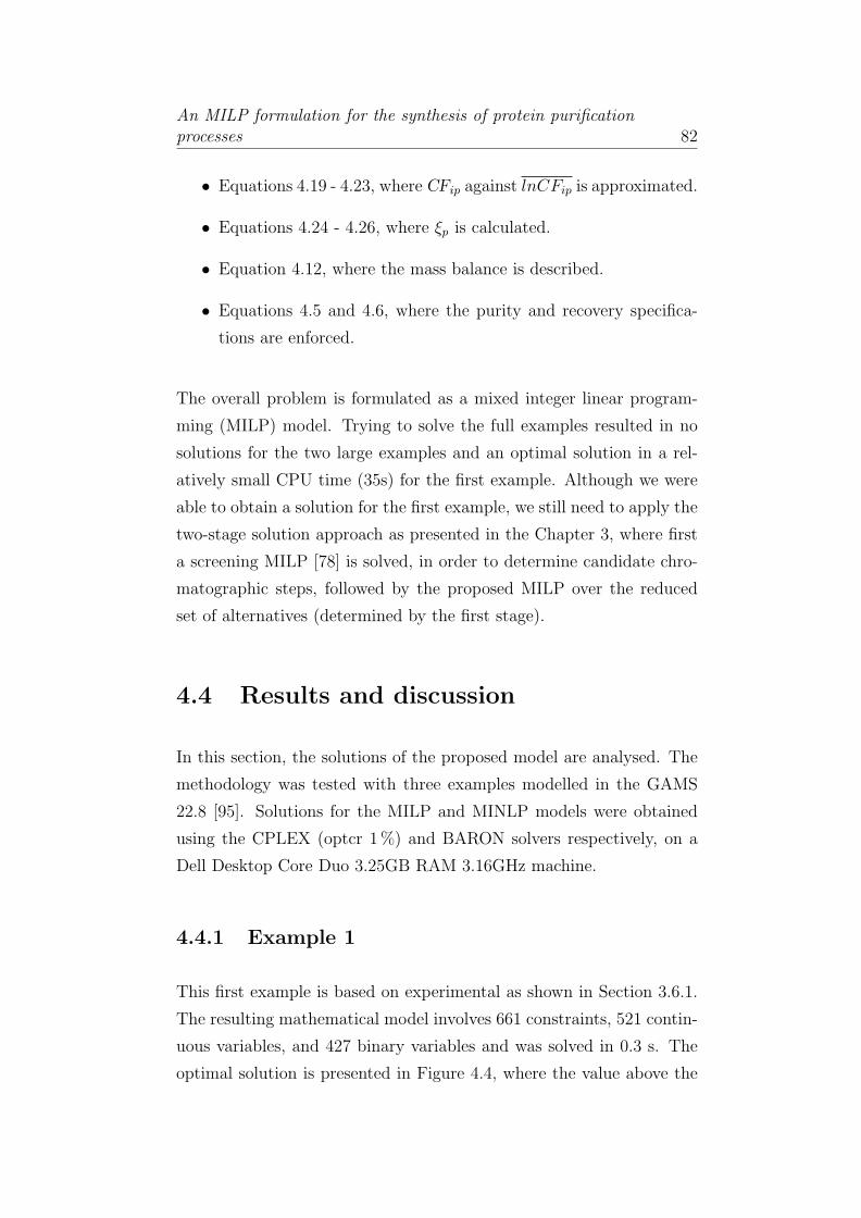
An MILP formulation for the synthesis of protein purificationprocesses 82
• Equations 4.19 - 4.23, where CFip against lnCFip is approximated.
• Equations 4.24 - 4.26, where ξp is calculated.
• Equation 4.12, where the mass balance is described.
• Equations 4.5 and 4.6, where the purity and recovery specifica-
tions are enforced.
The overall problem is formulated as a mixed integer linear program-
ming (MILP) model. Trying to solve the full examples resulted in no
solutions for the two large examples and an optimal solution in a rel-
atively small CPU time (35s) for the first example. Although we were
able to obtain a solution for the first example, we still need to apply the
two-stage solution approach as presented in the Chapter 3, where first
a screening MILP [78] is solved, in order to determine candidate chro-
matographic steps, followed by the proposed MILP over the reduced
set of alternatives (determined by the first stage).
4.4 Results and discussion
In this section, the solutions of the proposed model are analysed. The
methodology was tested with three examples modelled in the GAMS
22.8 [95]. Solutions for the MILP and MINLP models were obtained
using the CPLEX (optcr 1 %) and BARON solvers respectively, on a
Dell Desktop Core Duo 3.25GB RAM 3.16GHz machine.
4.4.1 Example 1
This first example is based on experimental as shown in Section 3.6.1.
The resulting mathematical model involves 661 constraints, 521 contin-
uous variables, and 427 binary variables and was solved in 0.3 s. The
optimal solution is presented in Figure 4.4, where the value above the

An MILP formulation for the synthesis of protein purificationprocesses 83
1st Step
0.25 0.983 AE pH 7.0
H I
1 0.980
Product 2nd Step Protein Mixture
Figure 4.4: Optimal flowsheet for purification of protein mixture(example 1)
arrow denotes the purity, and below refers to the recovery achieved. The
model was able to identify a solution that achieves purity sp = 0.983
and recovery fr = 0.98 for the target protein, for which two steps are
required: AE7, HI. The cut-points for AE7 were: xsAE7,dp = 0.004 and
xfAE7,dp = 0.143 and for HI: xsHI,dp = 0.002 and xfHI,dp = 0.220. In
Figure 4.5, the actual cut-points selected from the model are presented
on the chromatograms.
4.4.2 Example 2
This example utilises data available on [2] as shown in Section 3.6.2.
This example involves 2835 constraints, 2224 continuous variables, and
1824 binary variables and was solved in 4.2 s. The optimal solution is
presented in Figure 4.6, where a purity of sp = 0.951 and a recovery
of fr = 0.94 is achieved after three steps: AE6.5, AE8.5, HI. The cut-
points for AE6.5 were: xsAE6.5,dp = 0.012 and xfAE6.5,dp = 0.147 , for
AE8.5 were: xsAE8.5,dp = 0.013 and xfAE8.5,dp = 0.150 and for HI:
xsHI,dp = 0 and xfHI,dp = 0.198.
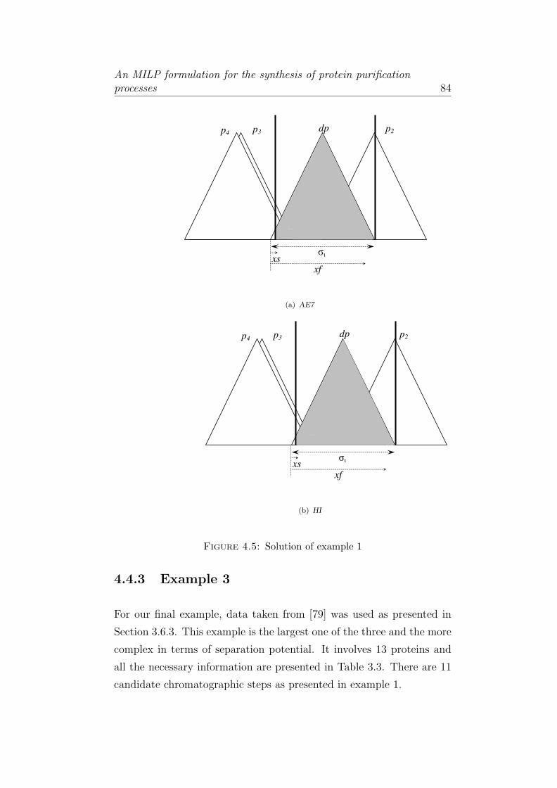
An MILP formulation for the synthesis of protein purificationprocesses 84
xs
p3
p2
p4
xf
dp
σι
(a) AE7
xs
p3
p2
p4
xf
dp
σι
(b) HI
Figure 4.5: Solution of example 1
4.4.3 Example 3
For our final example, data taken from [79] was used as presented in
Section 3.6.3. This example is the largest one of the three and the more
complex in terms of separation potential. It involves 13 proteins and
all the necessary information are presented in Table 3.3. There are 11
candidate chromatographic steps as presented in example 1.

An MILP formulation for the synthesis of protein purificationprocesses 85
1st Step
0.083 0.951 AE pH 6.5
1 0.940
AE pH 8.5
2nd Step
3d Step
HI
Product Protein Mixture
xs = 0.012
xf = 0.147
xs = 0.013
xf = 0.150
xs = 0
xf = 0.198
Figure 4.6: Optimal flowsheet for purification of protein mixture(example 2)
It takes 7.3 s to obtain the optimal solution and includes 3451 con-
straints, 2215 continuous variables, and 2705 binary variables. The
optimal solution achieved, is presented in Figure 4.7. Two steps are
required: AE7, CE4, HI in order to achieve a purity of sp = 0.937
and a recovery of fr = 0.903 for the target protein. The cut-points
for AE7 were: xsAE7,dp = 0.013 and xfAE7,dp = 0.134 , for CE4 were:
xsCE4,dp = 0.007 and xfCE4,dp = 0.133 and for HI: xsHI,dp = 0.013 and
xfHI,dp = 0.212.
4.4.4 Comparative results
In an effort to demonstrate the benefits of the proposed model, a com-
parison with the MINLP approach introduced in Chapter 3 is under-
taken. The MILP model was solved for five, ten and fifteen internal
knots for the piecewise linear approximation. All computational results
are summarised in Table 4.1, For all examples, ten internal knots were
sufficient to obtain the optimal solutions which was the same as the
ones determined by the MINLP described in Chapter 3. Using five
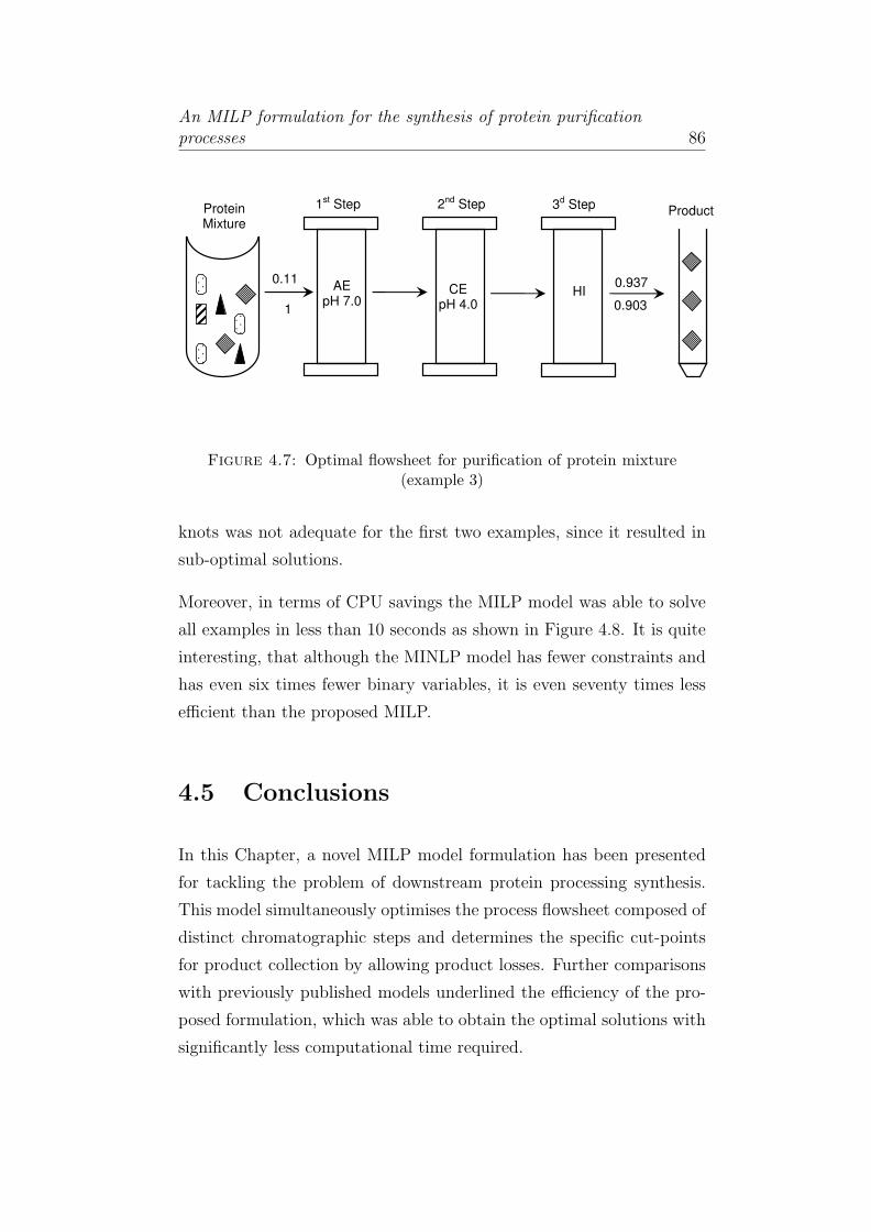
An MILP formulation for the synthesis of protein purificationprocesses 86
1st Step
0.11 0.937 AE pH 7.0
1 0.903
CE pH 4.0
2nd Step
3d Step
HI
Product Protein Mixture
Figure 4.7: Optimal flowsheet for purification of protein mixture(example 3)
knots was not adequate for the first two examples, since it resulted in
sub-optimal solutions.
Moreover, in terms of CPU savings the MILP model was able to solve
all examples in less than 10 seconds as shown in Figure 4.8. It is quite
interesting, that although the MINLP model has fewer constraints and
has even six times fewer binary variables, it is even seventy times less
efficient than the proposed MILP.
4.5 Conclusions
In this Chapter, a novel MILP model formulation has been presented
for tackling the problem of downstream protein processing synthesis.
This model simultaneously optimises the process flowsheet composed of
distinct chromatographic steps and determines the specific cut-points
for product collection by allowing product losses. Further comparisons
with previously published models underlined the efficiency of the pro-
posed formulation, which was able to obtain the optimal solutions with
significantly less computational time required.

An MILP formulation for the synthesis of protein purificationprocesses 87
Table 4.1: Computational statistics
example model NoCa NoCV/NoBV b CPU obj.(s) value
1
MINLPc 237 101/63 2.7 2MILPd 461 321/227 0.1 3MILPe 661 521/427 0.3 2MILPf 861 721/627 0.5 2MINLPc 1188 499/306 249 3MILPd 1980 1369/969 0.9 5
2 MILPe 2835 2224/1824 4.2 3MILPf 3690 3079/2679 5.2 3MINLPc 1454 605/375 501 3MILPd 2411 1665/1175 2.7 4
3 MILPe 3451 2705/2215 7.3 3MILPf 4491 3745/3255 117 3
a No of Constraintsb No of Continuous Variables/ No of Binary Variablesc Chapter 3d/e/f 5 knots/10 knots/15 knots
Example 1Example 2
Example 3
MILP
MINLP0
100
200
300
400
500
501
249
2.7
0.34.2
7.3
CP
U (
sec)
Figure 4.8: Comparison between MINLP presented in Chapter 3and proposed MILP

An MILP formulation for the synthesis of protein purificationprocesses 88
Even though there has been a significant improvement in computational
efficiency, still the model can not cope with the large examples that
include up to 13 protein and 21 candidate steps. In the next Chapter
an alternative approach is used in order to improve solution robustness
and avoid the two-stage solution approcah that was used here.

Chapter 5
An alternative MILP
formulation for the synthesis
of protein purification
processes
In this Chapter, we present an alternative MILP model for downstream
process synthesis. Instead of using piecewise linear approximation as
in the previous Chapter, we now use discrete recovery levels for the
product.
5.1 Introduction
In the previous Chapter we approximated the non-linearities that were
present in the model and although the efficiency of the model improved
significantly, the two-stage solution was not avoided for the larger ex-
amples. The objective was to be able to apply the developed models in
large mixtures that contain up to 20 contaminants.
89

An alternative MILP formulation for the synthesis of proteinpurification processes 90
The use of discrete recovery levels gives us the opportunity to take
advantage of the simplicity of the resulting linear models presented
below and obtain the optimal flowsheet in very small CPU times.
The basic assumption of the model is that each chromatographic peak
can be represented by an isosceles triangle. Again, the only necessary
input for this model are the mathematical correlations that relate the
retention time with the relevant physicochemical properties, respon-
sible for separation. The core for the modelling of chromatographic
separations remains the same as described in detail in Chapter 3.
5.2 Mathematical Models
In this section two alternative models will be described for solving the
problem of downstream protein processing.
5.2.1 Model 1
The objective function is to minimise the total number of steps from a
set of alternatives. Binary variable, Ei, is activated when a chromato-
graphic step i is selected.
Objective Function:
Min S =∑i
Ei (5.1)
The mass of each protein that remains after the first step is indicated by
equation 5.2. If the first technique is selected at starting recovery level,
ls, and finishing recovery level, lf, then the mass of protein p is reduced,
otherwise it is equal to the initial mass. Calculation of concentration
factors, CFip, is shown in Appendix C.

An alternative MILP formulation for the synthesis of proteinpurification processes 91
m1p =∑ls
∑lf
CF1,p,ls,lf ·λ1,ls,lf ·mop + (1−∑ls
∑lf
λ1,ls,lf ) ·mop ∀p
(5.2)
Similarly, in the following constraints, the mass of each protein for
i ≥ 2 is calculated. If step i is selected at starting recovery level ls
and finishing recovery level lf, the mass of protein p is calculated by
equation 5.3.
mip =∑ls
∑lf
CFi,p,ls,lf ·m1i−1,p,ls,lf +m2
i−1,p ∀p, i ≥ 2 (5.3)
If step i is selected, m1i−1,p,ls,lf is activated, otherwise m2
i−1,p is valid.
mi−1,p =∑ls
∑lf
m1i−1,p,ls,lf +m2
i−1,p ∀p, i ≥ 2 (5.4)
m1i−1,p,ls,lf ≤ mop · λi,ls,lf ∀p, i ≥ 2 (5.5)
m2i−1,p ≤ mop · (1−
∑ls
∑lf
λi,ls,lf ) ∀p, i ≥ 2 (5.6)
The following constraint ensures that for each i only one starting re-
covery level ls and one finishing recovery level lf are activated, if step
i is selected. ∑ls
∑lf
λi,ls,lf ≤ Ei ∀i (5.7)
In the two final constraints, purity, sp, and recovery, fr, specifications
are enforced.
mi,dp ≥ sp ·∑p′
mip′ ∀i = I (5.8)
mi,dp ≥ fr ·modp ∀i = I (5.9)

An alternative MILP formulation for the synthesis of proteinpurification processes 92
5.2.2 Model 2
The objective function is to minimise the overall number of steps from
a set of alternatives. Binary variable Ei is activated when a chromato-
graphic step i is selected.
Objective Function:
Min S =∑i
Ei (5.10)
The mass of each protein that remains after the first step is indicated
by equation 5.11. If the first technique is selected at starting recovery
level ls and finishing recovery level lf, then the mass of protein p is
reduced, otherwise it is equal to initial mass. As1,p,ls is the area that
lies below the starting cut point and Af1,p,lf is the area that lies below
the finishing cut point.
An example case on how the areas are related with the concentration
factors is shown in Figure 5.1. The first triangle considers the case
where only starting cut-point is considered and the shaded are repre-
sents the amount of contaminant remaining after the chromatographic
technique has been applied (Asi,p,ls). The second triangle represents the
case that only finishing cut-point is considered (Afi,p,lf ) and the final
case is where their difference is taken into account (Afi,p,lf−Asi,p,ls).Calculation of Asi,p,ls, Afi,p,lf along with concentration factors CFip is
shown in Appendix C.
m1p =
[∑lf
Af1,p,lf · µ1,lf −∑ls
As1,p,ls · λ1,ls
]·mop+(1−Ei)·mop ∀p
(5.11)
In the following constraint, the mass of each protein for i ≥ 2 is cal-
culated. If step i is selected at starting recovery level ls and finishing

An alternative MILP formulation for the synthesis of proteinpurification processes 93
(c) (a)
xsi,dp σι
xfi,dp
xsi,dp σι
(b)
xfi,dp
σι
Figure 5.1: Representation of areas
recovery level lf, the mass of protein p is calculated by Equation 5.12
where the first and second term of Equation 5.12 are active. These two
terms are similar to first term of Equation 5.3. The third term repre-
sents the case in which chromatographic step i has not been chosen,
hence protein is not reduced.
mip =∑lf
Afi,p,lf ·mf 1i−1,p,lf−
∑ls
Asi,p,ls ·ms1i−1,p,ls+m
2i−1,p ∀p, i ≥ 2
(5.12)
Similarly, in Equation 5.13 the mass of each protein p is calculated at
step i-1.
mi−1,p =∑lf
mf 1i−1,p,lf−
∑ls
ms1i−1,p,ls+m
2i−1,p ∀p, i ≥ 2 (5.13)
In equations 5.14 - 5.16, we have the calculation of terms mf 1i−1,p,lf ,
ms1i−1,p,ls, m
2i−1,p,lf which are activated depending on the selection of
chromatographic step i.

An alternative MILP formulation for the synthesis of proteinpurification processes 94
mf 1i−1,p,lf ≤ mop · µi,lf ∀p, i ≥ 2 (5.14)
ms1i−1,p,ls ≤ mop · λi,ls ∀p, i ≥ 2 (5.15)
m2i−1,p ≤ mop · (1− Ei) ∀p, i ≥ 2 (5.16)
The following two constraints ensure that binary variables µi,lf and λi,ls
are active only when a chromatographic step i is selected (Ei = 1).
∑lf
µi,lf ≤ Ei ∀i (5.17)
∑ls
λi,ls ≤ Ei ∀i (5.18)
In the two final constraints, purity, sp, and recovery, fr, specifications
are enforced.
mi,dp ≥ fp ·∑p′
mip′ ∀i = I (5.19)
mi,dp ≥ fr ·mop ∀i = I (5.20)
5.2.3 Discretisation method
As mentioned above the important item for these models is the discrete
recovery levels. In Figure 5.2, a chromatogram is represented by an
isosceles triangle and the peak width is discretised in a number of levels.
Given the recovery level selected the relevant concentration factor will
be calculated as presented in Appendix C.
In an effort to decide how many discrete levels should be provided in
advance, for both cut points xsi,dp, xfi,dp 5 and 10 recovery levels were
considered. (xsi,dp can vary from 0 to σi/10 and (xfi,dp can vary from
σi/2 to σi. The values used for the discretisation of both starting and
finishing cut-points are presented in Appendix C.
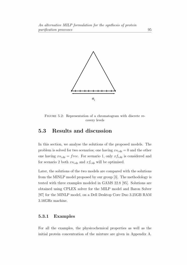
An alternative MILP formulation for the synthesis of proteinpurification processes 95
σi
Figure 5.2: Representation of a chromatogram with discrete re-covery levels
5.3 Results and discussion
In this section, we analyse the solutions of the proposed models. The
problem is solved for two scenarios; one having xsi,dp = 0 and the other
one having xsi,dp = free. For scenario 1, only xfi,dp is considered and
for scenario 2 both xsi,dp and xfi,dp will be optimised.
Later, the solutions of the two models are compared with the solutions
from the MINLP model proposed by our group [3]. The methodology is
tested with three examples modeled in GAMS 22.8 [95]. Solutions are
obtained using CPLEX solver for the MILP model and Baron Solver
[97] for the MINLP model, on a Dell Desktop Core Duo 3.25GB RAM
3.16GHz machine.
5.3.1 Examples
For all the examples, the physicochemical properties as well as the
initial protein concentration of the mixture are given in Appendix A.

An alternative MILP formulation for the synthesis of proteinpurification processes 96
All examples are based on literature data and they are the same ones
presented in the previous two chapters.
5.3.2 Scenario 1: xsi,dp = 0
In Table 5.1 the solutions from all examples and for xsip=0 are pre-
sented. First, the MINLP model described in Chapter 3 is presented
followed by the two MILP models proposed here. Both MILP models
were solved using 5 and 10 discrete points.
For example 1 and 2, solution obtained from the MINLP model agreed
with the ones from the MILP models. An interesting observation from
Table 5.1 is that for some cases, models 1 and 2 do not select the same
steps and this can happen because there is more than one solution that
can achieve the purity and recovery levels required (degeneracy).
For example 3, the MINLP selects 3 steps to achieve the requirements
while none of the MILP models can do that. To further investigate
this, example 3 was solved using 15, 20 and 25 discrete points for both
xsi,dp and xfi,dp. For 25 discrete points, 3 steps (AE8, CE4, HI) were
necessary to achieve a purity of fr = 0.931 and a recovery of fr = 0.90.
5.3.3 Scenario 1: xsi,dp = free
For this scenario, starting cut-point xsip is not fixed, but is a decision
variable. As expected, the purification flowsheet is improved with fewer
steps required as clearly presented in Table 5.2.
The most significant result was reported in example 2, where the num-
ber of steps is reduced from five to two. For this case, just 5 discrete
points were enough to achieve the same solutions as these obtained from
the MINLP.

An alternative MILP formulation for the synthesis of proteinpurification processes 97
5.3.4 Comparative results and computational statis-
tics
In this section, the proposed models are compared with the MINLP
model presented in Chapter 3 in terms of size and CPU time. In Table
5.3, CPU times are presented for all examples using the two proposed
MILPs for the scenarios described above and the MINLP.
In Figure 5.3, the CPU times along with computational statistics are
presented. For the MILP models the full size example is solved, while for
the MINLP the reduced problem is solved and yet the MINLP requires
the most of CPU time to obtain the solution. Moreover, the MINLP has
less binary and continuous variables but still takes more CPU time to
determine the optimal solution. Comparing the first MILP with second,
it is obvious that the second one is more efficient in computational time.
Binary and continuous variables along with the number of constraints
decrease significantly in the second MILP model proposed, hence CPU
time decreases as well.
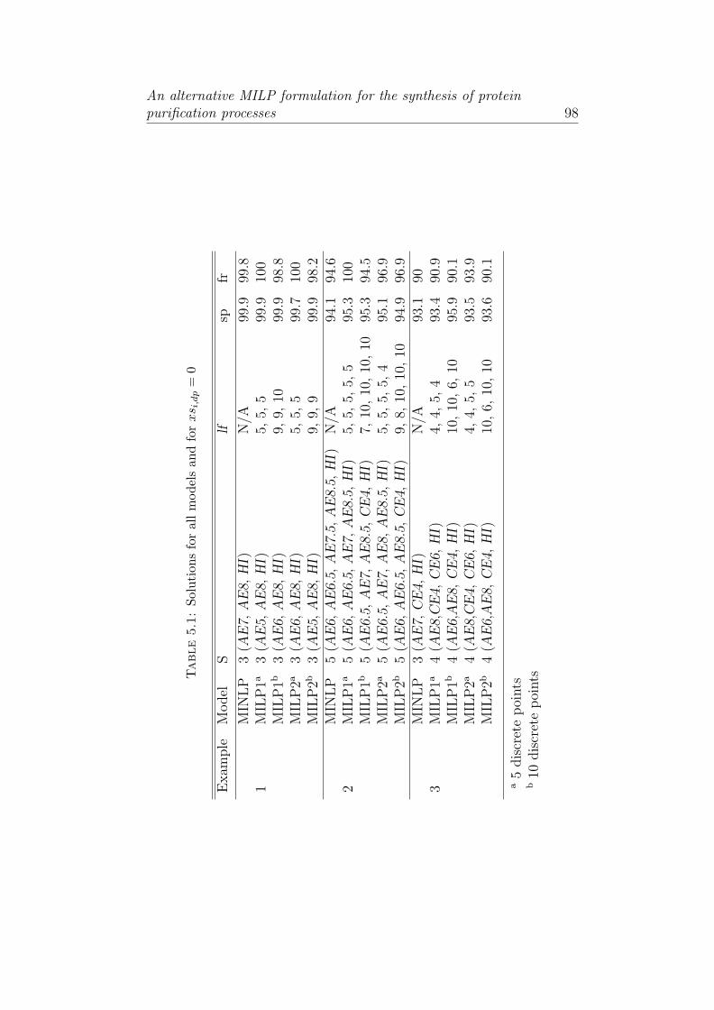
An alternative MILP formulation for the synthesis of proteinpurification processes 98
Table
5.1
:So
luti
ons
for
all
mod
els
and
forxs i,dp
=0
Exam
ple
Model
Slf
spfr
1M
INL
P3
(AE
7,A
E8,
HI)
N/A
99.9
99.8
MIL
P1a
3(A
E5,
AE
8,H
I)5,
5,5
99.9
100
MIL
P1b
3(A
E6,
AE
8,H
I)9,
9,10
99.9
98.8
MIL
P2a
3(A
E6,
AE
8,H
I)5,
5,5
99.7
100
MIL
P2b
3(A
E5,
AE
8,H
I)9,
9,9
99.9
98.2
2M
INL
P5
(AE
6,A
E6.
5,A
E7.
5,A
E8.
5,H
I)N
/A94
.194
.6M
ILP
1a5
(AE
6,A
E6.
5,A
E7,
AE
8.5,
HI)
5,5,
5,5,
595
.310
0M
ILP
1b5
(AE
6.5,
AE
7,A
E8.
5,C
E4,
HI)
7,10
,10
,10
,10
95.3
94.5
MIL
P2a
5(A
E6.
5,A
E7,
AE
8,A
E8.
5,H
I)5,
5,5,
5,4
95.1
96.9
MIL
P2b
5(A
E6,
AE
6.5,
AE
8.5,
CE
4,H
I)9,
8,10
,10
,10
94.9
96.9
3M
INL
P3
(AE
7,C
E4,
HI)
N/A
93.1
90M
ILP
1a4
(AE
8,C
E4,
CE
6,H
I)4,
4,5,
493
.490
.9M
ILP
1b4
(AE
6,A
E8,
CE
4,H
I)10
,10
,6,
1095
.990
.1M
ILP
2a4
(AE
8,C
E4,
CE
6,H
I)4,
4,5,
593
.593
.9M
ILP
2b4
(AE
6,A
E8,
CE
4,H
I)10
,6,
10,
1093
.690
.1
a5
dis
cret
ep
oints
b10
dis
cret
ep
oints

An alternative MILP formulation for the synthesis of proteinpurification processes 99
Table
5.2
:So
luti
ons
for
all
mod
els
and
forxs i,dp
=free
Exam
ple
Model
Sls
lfsp
fr
1M
INL
P2
(AE
7,H
I)N
/AN
/A98
.998
MIL
P1a
2(A
E7,
HI)
3,1
5,5
98.1
99.5
MIL
P1b
2(A
E7,
HI)
3,1
9,10
9899
.3M
ILP
2a2
(AE
7,H
I)3,
35,
598
.199
MIL
P2b
2(A
E7,
HI)
3,2
9,10
98.1
99.3
2M
INL
P3
(AE
6.5,
AE
8.5,
HI)
N/A
N/A
94.4
94.6
MIL
P1a
3(A
E6.
5,A
E8.
5,H
I)5,
3,1
4,5,
595
.494
.3M
ILP
1b3
(AE
6.5,
AE
8.5,
HI)
8,10
,10
8,10
,10
9694
.3M
ILP
2a3
(AE
6.5,
AE
8.5,
HI)
1,5,
69,
10,
1194
.394
.3M
ILP
2b3
(AE
6.5,
AE
8.5,
HI)
1,5,
69,
10,
1194
.394
.3
3M
INL
P3
(AE
8,C
E4,
HI)
N/A
N/A
93.1
90M
ILP
1a3
(AE
8,C
E4,
HI)
2,3,
24,
4,5
93.2
93.2
MIL
P1b
3(A
E8,
CE
4,H
I)5,
4,5
7,8,
994
.690
.6M
ILP
2a3
(AE
7,C
E4,
HI)
5,5,
14,
4,5
93.2
90M
ILP
2b3
(AE
8,C
E4,
HI)
2,4,
88,
7,10
93.1
90.1
a5
dis
cret
ep
oints
b10
dis
cret
ep
oints

An alternative MILP formulation for the synthesis of proteinpurification processes 100
Table 5.3: Comparative results for all models for both xsi,dp = 0and xsi,dp = free
xsi,dp = 0 xsi,dp = free
Example Model S CPU S CPU NoBV/NoCV/NoCa
(s) (s)
1MINLP 3 9 2 3.1 63/101/237MILP1b 3 0.2 2 0.5 286/1074/1138MILP1c 3 1.7 2 1.2 1111/4074/4138MILP2b 3 0.2 2 0.1 121/485/600MILP2c 3 1.1 2 0.7 231/885/989
2MINLP 5 233 3 277 306/499/1188MILP1b 5 2.3 3 16 536/4859/5073MILP1c 5 10.3 3 661 2111/18370/18573MILP2b 5 3.9 3 14.2 231/2170/2574MILP2c 5 15.2 3 2.2 441/3970/4374
3MINLP 3 285 3 505 375/605/1454MILP1b 4 0.5 3 5.4 1437/4286/3513MILP1c 4 7.4 3 201 1111/13263/3667MILP2b 4 0.5 3 1.6 121/1574/1858MILP2c 4 1.7 3 3.7 231/2874/3169
a Number of binary variables/ continuous variables/ constraintsb 5 discrete pointsc 10 discrete points
5.4 Conclusions
In this Chapter, two novel novel MILP model formulations have been
presented for tackling the problem of downstream protein processing
synthesis. This model simultaneously optimises the process flowsheet
composed of distinct chromatographic steps and determines the specific
cut-points for product collection by allowing product losses. Further
comparisons with previously published models underlined the efficiency
of the proposed formulation, which was able to obtain the optimal so-
lutions with significantly less computational time required.

An alternative MILP formulation for the synthesis of proteinpurification processes 101
Example 1Example 2
Example 3
MILP1
MILP2
MINLP
0
100
200
300
400
500
CP
U (
sec)
Figure 5.3: Comparison between MINLP [3] and proposed MILPs

Chapter 6
Computational
experimentation using
gPROMS
In this Chapter, the main mechanistic methodologies for chromato-
graphic processes will be discussed, followed by the specific model im-
plemented in gPROMS, along with the results obtained in an effort to
validate findings obtained in previous Chapters.
6.1 Introduction
As already mentioned, chromatography is a powerful separation method
that has been used for decades, initially as an analytical method and
later on as a purification method for complex mixtures. It is evidents
from Chapter 2 that a significant amount of research has been done in
an effort to synthesise and operate chromatographic steps in the best
possible way.
To do that, many researchers focused on mechanistic methods, where
the phenomena that take place into the column are considered. This
102

Computational experimentation using gPROMS 103
has not been a simple task since the process itself is quite complex,
but mainly because of the interactions between proteins within the
mixture. Several mathematical models are available in the literature
and are generally classified into two categories: plate models and rate
models. These models can be very powerful given that the necessary
parameters are known. In the next section, the main types of plate and
rate models are reviewed.
6.1.1 Plate model
This is the simplest model for chromatography and is based in the
assumption that the column is divided into a number of separate layers,
called theoretical plates. The concept of theoretical plates was first used
in distillation processes but was soon adapted by Martin and Synge [13].
Later on, other researchers [62, 98] used this type of model to optimise
ion exchange chromatography. The limitations of the plate model are
that it does not take into account adsorption kinetics, therefore can
not describe a multicomponent mixture where protein interactions are
significant.
6.1.2 Rate models
Rate models consider non-equilibrium conditions in the column and
take into account the contributions of mass transfer mechanisms. There
are many variations of the rate model such as the ideal model, the equi-
librium dispersive model, the transport dispersive model, the lumped
kinetic and the general rate model [99]. In the next section, some of
these models are discussed in detail.

Computational experimentation using gPROMS 104
6.1.2.1 Ideal model
The ideal model is the simplest model, where the chromatographic col-
umn is considered as one dimensional, hence the bed is considered ra-
dially homogeneous. Moreover, the mobile and stationary phase are
always in equilibrium [100]. The mass balance for each component p in
each bed i is described in Equation 6.1.
∂Cip∂t
+ F · ∂Csip∂t
+ u · ∂Cip∂x
= 0 ∀i, p (6.1)
where the first term is the rate of accumulation of component p in
step i within the particle, the second term is the rate of accumulation
of component p in step i in the mobile phase, the third is the rate
transport through convection, F is the phase ratio, u is the intersitial
velocity, calculated by the following equation.
u =4 · FcεB ·D2
(6.2)
where Fc is the eluent flowrate, εB is the bed voidage and D is the
column diameter.
This model is still used but mainly for single columns or binary mix-
tures, mainly because it can accommodate protein interactions in com-
plex mixtures [42, 101].
6.1.2.2 Equilibrium-dispersive model
In this case, the mass transfer is fast but not infinitely fast, therefore
contributions due to non-linear equilibrium can be described by an ap-
parent axial dispersion coefficient term Daxip [100]. The mass balance
for each component p in each bed i is described in Equation 6.3.

Computational experimentation using gPROMS 105
Moreover the equilibrium dispersive model is based on the following
assumptions:
• Packed bed is assumed to be isothermal and uniformly packed.
• Radial velocity is negligible.
• Concentration profiles are assumed to be one-dimensional.
• Diffusion coefficients of solutes in both mobile and stationary
phase are considered.
• Adsorption equilibrium is supposed to be instantaneous and can
be described by the axial dispersion term [100].
∂Cip∂t
+ F · ∂Csip∂t
+ u · ∂Cip∂x
= Daxip ·∂2Cip∂x2
∀i, p (6.3)
where last term is the rate of transport by axial dispersion and Daxip
is the axial dispersion coefficient.
The equilibrium dispersive model is widely used in literature [47, 102,
103]. Teoh et al. [47], applied this model for a high performance liquid
chromatography of an aromatic mixture of four components. Vaquez-
Alvarez et al. [102], employed the same model for an ion exchange
chromatography of a four protein mixture and Marcus et al. [103] for
the separation of protein monomers from dimers.
Adsorption equilibria
The adsorption mechanism that describes the phenomena present in-
side the chromatographic column is mathematically expressed by an
isotherm relationship. In the following paragraphs, some examples of
isotherms are discussed.

Computational experimentation using gPROMS 106
Linear adsorption isotherm
This is the simplest theoretical isotherm used in the modelling of liq-
uid chromatography. In this type of isotherm, the components in the
mixture behave independently of each other. The solute concentration
in the stationary phase, Csip, is related to the one of the mobile phase,
Cip, with a constant, αip. The mathematical form for this isotherm is
presented in Equation 6.4.
Csip = aip · Cip ∀i, p (6.4)
Langmuir isotherm
This is the most widely used theoretical isotherm employed for mod-
elling of chromatographic processes. The components are assumed to
be adsorbed on fixed number of sites and each site may accept only one
compound. There is no interaction between adsorbed compounds and
a local equilibrium is assumed between the stationary and the mobile
phase [100, 104].
The mathematical form for this isotherm is presented in Equation 6.5.
Csip =aip · Cip
1 + bip · Cip∀i, p (6.5)
where aip and bip are coefficient for each component p and each bed i.
Competitive Langmuir isotherm
When there is a multicomponent mixture, the amount of each com-
ponent adsorbed at equilibrium is smaller than if that component was
alone. The mathematical form for this isotherm is presented in Equa-
tion 6.6.
Csip =aip · Cip
1 +∑p′bip′ · Cip′
∀i, p (6.6)

Computational experimentation using gPROMS 107
6.1.2.3 General rate model
The general rate model is the most complex one because it takes into
account all the phenomena that may influence the column such axial
dispersion, external mass transfer, intraparticle diffusion and the ad-
sorption kinetics. It is the most comprehensive model in literature,
however it requires the determination of many parameters a priori. It
consists of two partial differential equations. The first one is Equa-
tion 6.3 and the second one is the following equations where the mass
balance for each component p in the pore phase is given.
εp ·∂Cpip∂t
+ (1− εp) ·∂Csip∂t
= εp ·Daxip ·[
1
r2
∂
∂r
(r2 · ∂Cpip
∂r
)]∀i, p
(6.7)
where the first term is the rate of accumulation in the pore liquid, the
second the rate of accumulation on the solid surface and the right hand
side is related to the rate of radial diffusion. εp is the particle porosity.
For the second term of Equation 6.7 we need to calculate the rate of
adsorption and this is why we need the following equation.
∂Cpsip∂t
= kap · (Λp −∑p
Cpsip) · Cpip − kdp · Cpsip ∀i, p (6.8)
where kap and kdp are the adsorption and desorption rate constants for
each component p, Λp −∑
pCpsip are the available free sites, where Λp
is the adsorption saturation capacity for each component p.
6.1.3 Comparing chromatographic models
Plate and rate models were described in detail in the sections above.
The plate model is able to predict elution profiles and was popular

Computational experimentation using gPROMS 108
when computational efficiency was limited. However, even at that time
it was clear that the plate model had limited capabilities because of
its simplicity. On the contrary rate models are very comprehensive
models that can thoroughly describe the phenomena taking place in
the column. In the two extremes, we have the ideal model and general
rate model with the first one being simplistic and the last one being to
detailed and difficult to accommodate because of the requirements in
input parameters. The equilibrium dispersive model will be employed
because it provides a sufficient understanding of the process and does
not require so many parameters.
6.2 Model selection
After reviewing the several available mathematical models the decision
was to use the equilibrium dispersive model. It has been proven to
be efficient and less demanding in terms of necessary input parameters
[44]. This type of model has been widely used in literature [47], [102]
and was first described by Bellot and Condoret in 1991 [105].
The first equation is the material balance (Equation 6.3) as described
earlier, along with the Langmuir isotherm as described in Equation 6.5.
The initial and boundary conditions are given from Equations 6.9 -
6.11.
Initial Condition
Cip|t0,x = 0 ∀i, p, x ∈ (0, L) (6.9)
Boundary Conditions
∂Cip∂x
∣∣∣x=L
= 0 ∀i, p (6.10)

Computational experimentation using gPROMS 109
Cip|x=0 = Cinip ∀i (6.11)
where for the first chromatographic step i=1 Cinip = Cfeed and Cin
i =
Cout(i− 1) ∀ i > 1.
Since the system we are considering is a multicolumn one, the output of
each chromatographic step becomes the input of the next. A graphical
explanation of that is presented in Figure 6.1.
STEP i-1Cfeed
STEP i STEP i+1Cout = CfeedCout = Cfeed
Figure 6.1: Mass flow in the multicolumn system
A shown in Figure 6.1 a new variable is introduced, Coutip , which is the
amount of protein that is collected at the specific integral and is defined
by Equation 6.12.
Coutip =
∫ tfinish
tstart
Cip|x=Ldt (6.12)
In Figure 6.2, the necessary intervals are presented. T1 is the interval
where the column is fed with the mixture, followed by T2 in which no
action takes place, but at its end the starting cut-point presented in
Chapter 3 occurs and finally T3 which is the collection interval and at
its end is where finishing cut-point occurs.
Finally, the purity and recovery are calculated by Equations 6.13 and
6.14.
Calculation of purity
Rip =Coutip
Cinip
∀i, p = dp (6.13)

Computational experimentation using gPROMS 110
tfeed tstart tfinish
T1
T2 T
3
Figure 6.2: Graphical representation of a chromatogram and timeintegrals
Calculation of recovery
Pip =Couti,p∑
p′ Coutip′∀i (6.14)
6.3 Case study and numerical simulation
The case study considered is four-protein mixture and four candidate
chromatographic steps. The data used for this model are shown in
Tables 6.1 and 6.2. In the first table the data related to the column are
presented. The values are the same as the ones from Teoh’s paper [47].In
Table 6.2 the Langmuir parameters, αip, βip, and the axial dispersion
coefficients, Daxip are presented.
The system of equations described above was implemented using gPROMS
[106]. The axial domain was discretized using 3rd order orthogonal col-
location with 200 uniform elements (OCFEM). After running the sim-
ulation for each chromatographic step individually, the retention times

Computational experimentation using gPROMS 111
Table 6.1: Column parameters used for the simulation
Column Length 0.25 mPhase ratio 0.38Inertial velocity 0.027 m/s
Table 6.2: Langmuir parameters used for the simulation
αip βip Daxip αip βip DaxipBed 1 Bed 2
target protein 1100 0.09 5.1E-5 700 0.08 5.2E-5contaminant 1 700 0.1 5.0E-5 1000 0.07 4.8E-5contaminant 2 1300 0.08 5.2E-5 1350 0.09 4.9E-5contaminant 3 1400 0.07 5.3E-5 1400 0.1 5.0E-5
Bed 3 Bed 4target protein 850 0.07 9.0E-5 950 0.09 9.0E-5contaminant 1 750 0.1 8.0E-5 1050 0.08 8.0E-5contaminant 2 950 0.08 6.0E-5 850 0.1 6.0E-5contaminant 3 1050 0.1 5.0E-5 1150 0.08 5.0E-5
for each component p as well as the relative peak width, σi, were cal-
culated and the values are given in Table 6.3. Moreover, the output of
gPROMS simulation for the individual columns are presented in Ap-
pendix D. In all four Figures, the chromatogram in red is the target
protein and the ones in black, green and blue are considered to be the
contaminants.
Table 6.3: Parameters used in GAMS
trip σip trip σip
Bed 1 Bed 2target protein 3760 2910 2390 1970contaminant 1 2390 1930 3420 2620contaminant 2 4440 3420 4620 3440contaminant 3 4780 3670 4780 3590
Bed 3 Bed 4target protein 2840 2970 3170 3270contaminant 1 2514 2530 3530 3620contaminant 2 3230 2750 2890 2500contaminant 3 3590 2780 3930 3010

Computational experimentation using gPROMS 112
Using the data presented above, we were able to run the MINLP and
MILP models presented in Chapter 3, 4 and 5. Purity and recovery
requirements are set to 99 % and 97 % respectively.
6.4 Results and Discussion
6.4.1 GAMS
The MINLP model described in Chapter 3 along with the MILP models
described in Chapters 4 and 5 were implemented in GAMS and solved,
for a purity of sp = 0.99 and a recovery of fr = 0.97. For all models the
chromatographic steps selected were: Bed1 and Bed2. The cut-points
for all the models are presented in table 6.4.
Table 6.4: Cut-points resulting from GAMS models
Bed 1 Bed 2
xsBed1,dp xfBed1,dp xsBed2,dp xfBed2,dpMINLP Section 3.4 230 2855 0 1788MILP1 Section 4.2 291 2910 0 1879MILP2 Section 5.2.2 290 2910 0 1880
These cut-points were used as part of schedule in gPROMS simulation
for validation.
6.4.2 gPROMS
After implementing these scheduling times in gPROMS, the purity and
the recovery achieved are presented in table 6.5.
The output of gPROMS is presented in Figure 6.3 but only for the
MINLP model, where the first graph shows the first bed. As expected,
there are all four proteins in the mixture and after the cut-points are
applied then in the second bed, only the target protein and one of

Computational experimentation using gPROMS 113
Table 6.5: Purities and recoveries achieved by gPROMS
Purity Recovery
MINLP Section 3.4 99.5 % 96 %MILP1 Section 4.2 99 % 97 %MILP2 Section 5.2.2 99 % 97 %
the contaminants are left, because the other two contaminants were
discarded during the first step.
Below, the final two figures present how does purity and recovery change
during time. In Figure 6.4, the black line represents the first bed and the
red line the second bed. Initially the purity is very high and gradually
decreases until it reaches 33 %. This happens because at the beginning
as it is shown in Figure 6.3, only the target protein is collected, therefore
the purity is high, but then the contaminants start occuring and the
purity drops. In the second bed, the purity again starts from a high
values because the target protein is the first protein to elute from the
column and remains high because the contaminant still in the mixture
is never collected. Similarly, in Figure 6.5, we have a gradual increase
of the recovery of the target protein until it reaches the final 96 %.

Computational experimentation using gPROMS 114
(a) Bed 1
(b) Bed 2
Figure 6.3: gPROMS output for two-step simulation

Computational experimentation using gPROMS 115
Fig
ure
6.4
:gP
RO
MS
outp
uton
puri
ty

Computational experimentation using gPROMS 116
Fig
ure
6.5
:gP
RO
MS
outp
uton
reco
very

Computational experimentation using gPROMS 117
6.5 Conclusions
In this Chapter, the main mechanistic models available in literature
were reviewed and the equilibrium dispersive model was selected for the
validation process of the models described in Chapter 3, 4, 5. After, the
selected model was used to implement a case study in gPROMS and
the results were used as the input in all developed models described in
Chapter 3, 4, 5. After the selected steps and the respective cut-points
were determined from GAMS, the models were simulated in gPROMS
and the purity and recovery were calculated and validated. Values of
both purity and recovery have a maximum error of 1 %.
Chapter 7
Conclusions and future
directions
The aim of this thesis was to investigate different methodologies in
order to enhance operation and synthesis of chromatographic purifica-
tion processes. Towards that goal, a number of mathematical models
were developed and their results were presented in the previous chap-
ters. In the following section, the main contributions of the thesis are
summarised followed by new directions for future work.
7.1 Contributions of the thesis
This thesis focused on the optimisation of downstream processes in
biopharmaceutical plants. In Chapter 1, some basic background infor-
mation were presented for the biopharmaceutical industry in today’s
market, followed by the description of a typical flowsheet. Chromatog-
raphy was targeted as the bottleneck of downstream processing and
the main source of cost and was the focus of this work. Next, a brief
history of how chromatography has evolved in the last decades from an
analytical process to a full scale industrial process, followed.
118

Conclusions and Future Work 119
In Chapter 2, current approaches in the area of of downstream process
synthesis and operation were highlighted. Based on some previsously
developed work [78, 79] for the synthesis of purification processes, we
then presented an MINLP approach that can take into account prod-
uct losses and minimises the number of chromatographic steps in the
purification process. This framework not only optimises the flowsheet
but also selects the timeline in which the product is selected, there-
fore operating conditions can also be manipulated for the benefit of the
process. This MINLP model was solved using a two-stage process and
tested through three illustrative examples.
Next, in Chapter 4, and by applying piecewise linear approximation,
the MINLP model was linearised in order to improve computational
efficiency. With this new model, we were able to avoid the two-stage
procedure for the first example, but not for the two larger examples.
Nevertheless, quality of the solution was indicative of a successful ap-
proximation.
Later on, in Chapter 5, two models were developed using discrete re-
covery levels for the target protein. These models were also tested with
the same three examples and they were able to cope with the full prob-
lem size up to 21 candidate steps and 13-protein mixtures. Finally,
in Chapter 6, models based on first principles were reviewed and the
equilibrium dispersive model was implemented in the simulation plat-
form gPROMS [106]. Purities and recoveries were compared with the
ones from the mathematical models from GAMS and the error did not
exceed 1%.
7.2 Recommendations for future work
There are a number of possible future directions related to the synthesis
and operation of chromatographic processes:

Conclusions and Future Work 120
7.2.1 Additional chromatographic processes
One obvious direction would be the addition of more chromatographic
steps. In Chapter 1, we spoke about the different principles of separa-
tion. Apart from ion-exchange chromatography (IEX) and hydropho-
bic interaction (HIC) which are used in this thesis, size exclusion (SE),
affinity chromatography (AC) and mixed mode (MMC)could be con-
sidered. The only constraint for this suggestion is the lack of experi-
mental data and the relevant mathematical correlations. For IEX, we
have the mathematical correlation relating retention time with charge
and molecular weight. For AC and MMC, these correlations are quite
a challenge mainly because in the first case the adsorption mechanism
is the result of molecular recognition which is not easy to be quantified
and for the second case because one of the two separation principles will
be more significant than the other and again this needs to be somehow
quantified.
7.2.2 Model enhancement
Another direction would be to extend the model itself. As mentioned
in Chapter 2, the overall aim is to model the whole biopharmaceutical
process in order to predict operating conditions, different configurations
and scheduling. Taking small steps, we could try and incorporate some
operating parameters that affect chromatographic performance, such
as flowrate or ionic strength. Again the constraint is that there are no
direct correlations that relate retention time with flowrate.
Since the focus of this project was downstream processes, an idea would
be to include processes such as of filtration, centrifugation as part of the
flowsheet and try to optimise the flowsheet by minimising the number
of units.

Conclusions and Future Work 121
7.2.3 Economic evaluation
This can be incorporated either in the objective function by just adding
an approximate cost of each purification step, but it can be also done
in great detail using cost of goods (COG) strategies, where resin cost,
buffer cost, column cost and resin lifetime are taken into account. This
can have a significant improvement in the optimisation by improving
the accuracy of the results.
7.2.4 Experimental validation
In this thesis, we used computational experimentation in order to vali-
date the mathematical models developed. The ideal methodology would
be to actually run the experiments for the examples we are using, by
running them though the specific chromatographic columns that have
been selected and compare the purities and recoveries achieved. These
are straightforward experiments using a liquid chromatography method
that is available.
7.2.5 Mathematical correlation predictions
The input of the developed model is the mathematical correlations that
have been experimentally derived, by running liquid chromatography
to determine the retention time and by relating that to charge, molec-
ular weight and hydrophobicity. These correlations have been derived
mainly by the use of partial least square methods. Given that new ex-
perimental data can become available more sophisticated methods such
as support vector regression or neural networks can be applied to cre-
ate a database of mathematical correlations that can predict retention
times given the parameters responsible for separation and possibly the
column specifics.

Conclusions and Future Work 122
7.3 Summary and main contributions
This thesis has developed and presented a number of optimisation-based
models for the synthesis and operation of chromatographic processes.
Three illustrative examples have been used to verify the models. The
main contributions from this thesis are:
• a mixed integer non-linear programming mathematical model for
minimising the number of chromatographic steps and determining
the timeline at which the product is collected;
• three mixed integer linear programming mathematical models
solving the same problem; and
• validation of the models through computational experimentation
using gPROMS.

Appendix A
Calculated KDip and DFip for
MINLP model
Below, six tables follow, containing all the calculations for dimensionless
retention times KDip and deviation factors DFip, for all three examples.
KDip and DFip were calculated based on equations 3.2-3.6 and 3.7
respectively, as presented in section 3.3.
Table A.1: Dimensionless retention times in example 1
KDip dp p1 p2 p3
AE4 0 0 0 0AE5 0.015 0.1 0.154 0AE6 0.1 0.174 0.233 0AE7 0.132 0.206 0.272 0AE8 0.152 0.215 0.270 0CE4 0.073 0.124 0.161 0.209CE5 0 0 0 0.208CE6 0 0 0 0.211CE7 0 0 0 0.206CE8 0 0 0 0.144HI 0.427 0.64 0.4 0.407
123
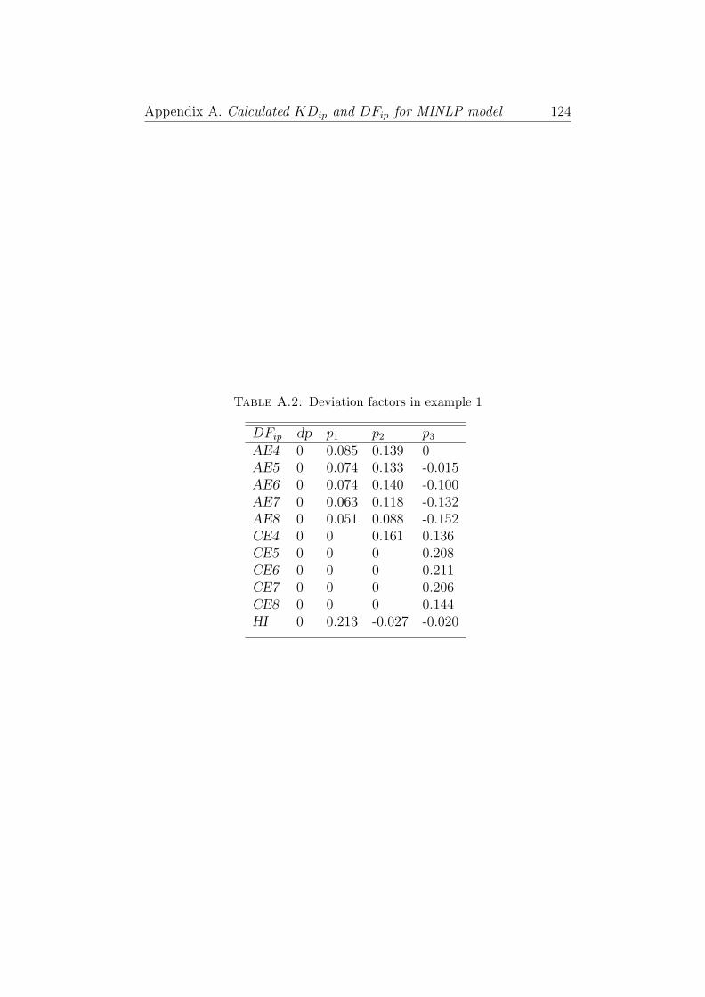
Appendix A. Calculated KDip and DFip for MINLP model 124
Table A.2: Deviation factors in example 1
DFip dp p1 p2 p3
AE4 0 0.085 0.139 0AE5 0 0.074 0.133 -0.015AE6 0 0.074 0.140 -0.100AE7 0 0.063 0.118 -0.132AE8 0 0.051 0.088 -0.152CE4 0 0 0.161 0.136CE5 0 0 0 0.208CE6 0 0 0 0.211CE7 0 0 0 0.206CE8 0 0 0 0.144HI 0 0.213 -0.027 -0.020
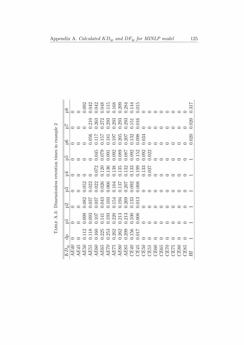
Appendix A. Calculated KDip and DFip for MINLP model 125
Table
A.3
:D
imen
sion
less
rete
ntio
nti
mes
inex
ampl
e2
KDip
dp
p1
p2
p3
p4
p5
p6
p7
p8
AE
400
00
00
00
00
AE
450
00
00
00
00
AE
500.
112
0.09
90.
082
0.05
20
00
00.
092
AE
550.
118
0.09
30.
037
0.02
20
00.
056
0.21
00.
042
AE
600.
160
0.10
70.
037
0.02
20.
072
0.04
50.
117
0.26
30.
042
AE
650.
225
0.14
10.
043
0.02
60.
120
0.07
90.
157
0.27
20.
048
AE
700.
253
0.19
30.
103
0.06
60.
136
0.09
10.
181
0.29
30.
115
AE
750.
262
0.22
00.
154
0.10
40.
138
0.09
20.
197
0.29
30.
168
AE
800.
262
0.21
30.
194
0.13
70.
135
0.08
90.
205
0.29
30.
209
AE
850.
299
0.21
30.
269
0.20
70.
132
0.08
70.
207
0.29
30.
284
CE
400.
156
0.10
00.
133
0.09
20.
133
0.09
20.
132
0.15
10.
144
CE
450.
017
0.00
80.
013
0.00
80.
199
0.15
20.
098
0.01
60.
015
CE
500
00
00.
133
0.09
20.
034
00
CE
550
00
00.
037
0.02
20
00
CE
600
00
00
00
00
CE
650
00
00
00
00
CE
700
00
00
00
00
CE
750
00
00
00
00
CE
800
00
00
00
00
CE
850
00
00
00
00
HI
11
11
11
0.02
00.
020
0.31
7

Appendix A. Calculated KDip and DFip for MINLP model 126
Table
A.4
:D
evia
tion
fact
ors
inex
ampl
e2
KDip
dp
p1
p2
p3
p4
p5
p6
p7
p8
AE
400
00
00
00
00
AE
450
00
00
00
00
AE
500
-0.0
13-0
.03
-0.0
6-0
.112
-0.1
12-0
.112
-0.1
12-0
.020
AE
550
-0.0
25-0
.081
-0.0
96-0
.118
-0.1
18-0
.062
0.09
2-0
.076
AE
600
-0.0
53-0
.123
-0.1
38-0
.088
-0.1
15-0
.043
0.10
3-0
.118
AE
650
-0.0
84-0
.182
-0.1
99-0
.105
-0.1
46-0
.068
0.04
7-0
.177
AE
700
-0.0
6-0
.150
-0.1
87-0
.117
-0.1
62-0
.072
0.04
0-0
.138
AE
750
-0.0
42-0
.108
-0.1
58-0
.124
-0.1
70-0
.065
0.03
1-0
.094
AE
800
-0.0
49-0
.068
-0.1
25-0
.127
-0.1
73-0
.057
0.03
1-0
.053
AE
850
-0.0
86-0
.03
-0.0
92-0
.167
-0.2
12-0
.092
-0.0
06-0
.015
CE
400
-0.0
56-0
.023
-0.0
64-0
.023
-0.0
64-0
.024
-0.0
05-0
.012
CE
450
-0.0
09-0
.004
-0.0
090.
182
0.13
50.
081
-0.0
01-0
.002
CE
500
00
00.
133
0.09
2-0
.034
00
CE
550
00
00.
037
0.02
20
00
CE
600
00
00
00
00
CE
650
00
00
00
00
CE
700
00
00
00
00
CE
750
00
00
00
00
CE
800
00
00
00
00
CE
850
00
00
00
00
HI
00
00
00
-0.9
8-0
.98
-0.6
83

Appendix A. Calculated KDip and DFip for MINLP model 127
Table
A.5
:D
imen
sion
less
rete
ntio
nti
mes
inex
ampl
e3
KDip
dp
p1
p2
p3
p4
p5
p6
p7
p8
p9
p10
p11
p12
AE
400
00
00
00.
176
00.
020
00
00
AE
500
00
00.
100
00.
178
0.18
80.
050
00.
149
00
AE
600.
039
00
00.
173
00.
212
0.21
50.
104
0.28
70.
227
00.
048
AE
700.
077
00
0.10
20.
206
00.
287
0.27
00.
120
0.31
60.
253
00.
114
AE
800.
101
00
0.14
80.
214
00.
291
0.30
30.
132
0.32
90.
265
00.
150
CE
400.
128
0.21
80.
238
0.26
90.
128
0.28
90.
000
0.12
60
0.26
00.
163
0.25
60.
178
CE
500.
080
0.21
60.
204
0.18
10
0.28
70
00
0.18
70
0.18
20.
092
CE
600
0.21
50.
184
0.10
30
0.28
70
00
00
0.15
30
CE
700
0.21
50.
147
00
0.28
30
00
00
0.10
90
CE
800
0.14
90.
090
00
0.26
60
00
00
0.00
30
HI
0.70
20.
629
0.81
80.
392
0.70
10.
655
0.87
10.
290
0.64
90.
075
0.78
00.
682
0.50
3

Appendix A. Calculated KDip and DFip for MINLP model 128
Table
A.6
:D
evia
tion
fact
ors
inex
ampl
e3
DFip
dp
p1
p2
p3
p4
p5
p6
p7
p8
p9
p10
p11
p12
AE
400
00
00
00.
176
00.
020
00
00
AE
500
00
00.
100
00.
178
0.18
80.
050
00.
149
00
AE
600
-0.0
39-0
.039
-0.0
390.
134
-0.0
390.
173
0.17
60.
065
0.24
80.
188
-0.0
390.
009
AE
700
-0.0
77-0
.077
0.02
50.
129
-0.0
770.
210
0.19
30.
043
0.23
90.
176
-0.0
770.
037
AE
800
-0.1
01-0
.101
0.04
70.
113
-0.1
010.
190
0.20
20.
031
0.22
80.
164
-0.1
010.
049
CE
400
0.09
00.
110
0.14
10
0.16
1-0
.128
-0.0
02-0
.128
0.13
20.
035
0.12
80.
050
CE
500
0.13
60.
124
0.10
1-0
.080
0.20
7-0
.080
-0.0
80-0
.080
0.10
7-0
.080
0.10
20.
012
CE
600
0.21
50.
184
0.10
30
0.28
70
00
00
0.15
30
CE
700
0.21
50.
147
00
0.28
30
00
00
0.10
90
CE
800
0.14
90.
090
00
0.26
60
00
00
0.00
30
HI
0-0
.073
0.11
6-0
.310
-0.0
01-0
.047
0.16
9-0
.412
-0.0
53-0
.627
0.07
8-0
.020
-0.1
99

Appendix B
Piecewise linear
approximation
Below there is a description of the optimal approximations of single-
dimensional nonlinear functions by piecewise linear functions as de-
scribed by [96]. The approach uses a discrete representation of the
non-linear function described by pairs (xi, fi), i ∈ Q = 1, 2, ...nQ, where
Q is the predefined sampling set. Binary variable Wij is equal to 1 if
i ∈ Q and j ∈ Q are two consecutive points, otherwise is 0. N is the
number of knots given a priori.
At most one one polynomial piece of the approximating function may
begin and one piece may end in each of the points in Q.
∑j∈Qj>i
Wij ≤ 1 ∀i ∈ Q|i > 1 (B.1)
∑i∈Qj>i
Wij ≤ 1 ∀j ∈ Q|j > nQ (B.2)
The first and last points of Q are necessarily part of the knots.
129

Appendix B. Piecewise linear approximation 130
∑j∈Qj>i
Wij = 1 ∀i = 1 (B.3)
∑i∈Qj>i
Wij = 1 ∀j = nQ (B.4)
Any knot has to be both the start and the end of a polynomial piece of
the approximating function and the end of another (except of the first
and last ones).
∑i∈Qk>i
Wik =∑i∈Qj>k
Wkj ∀k > 2...nQ − 1 (B.5)
The approximating function is predefined to have N internal knots.
∑i∈Q
∑j∈Qj>i
Wij = N − 1 (B.6)
The values of the approximating function are defined by the following
set of constraints.
fPk =∑i∈Qi<k
∑j∈Qj>k
[(xk − xi) · fj + (xj − xk) · fi](xj − xi)
·Wij ∀k ∈ Q
(B.7)
To measure the quality of the approximation, the 1-norm of distance
between the vectors describing the original function and the piecewise
linear approximation. The objective function is to minimise this norm
and is given by the following constraints.

Appendix B. Piecewise linear approximation 131
Z =∑i∈Q
zi (B.8)
zi ≥ (fi − fPi )∀i ∈ Q (B.9)
zi ≥ −(fi − fPi )∀i ∈ Q (B.10)

Appendix C
Calculation of concentration
factors
STEP 1: Generation of cut-points, xsi,dp, xfi,dp
STEP 2: Calculation of shifted cut-points xsip.
xsip = xsi,dp −DFip ∀i, p 6= dp (C.1)
xf ip = xfi,dp −DFip ∀i, p 6= dp (C.2)
STEP 3: Correction of shifted cut points xsip.
• If xsip < 0 → ∆sip = 0 & xfip < 0 → ∆fip = 0
• If xsip > σi → ∆sip = σi & xfip > σi → ∆fip = σi
• If 0 ≤ xsip ≤ σi & 0 ≤ xfip ≤ σi → ∆fip = xfip
132
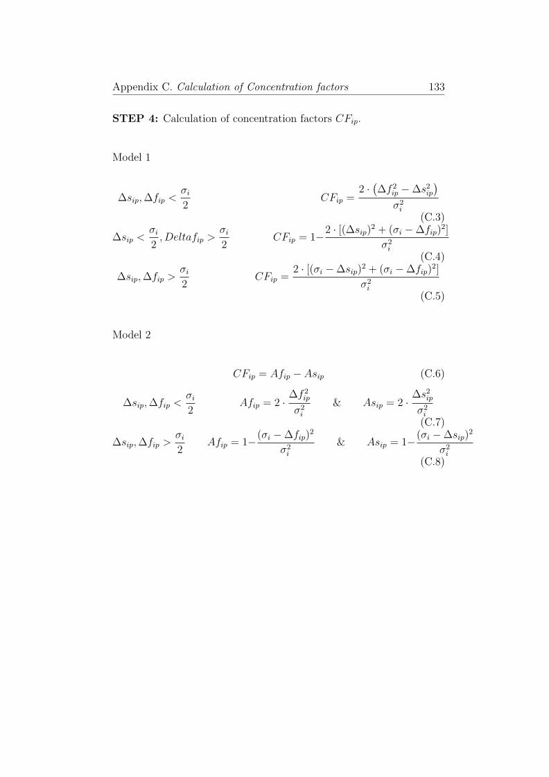
Appendix C. Calculation of Concentration factors 133
STEP 4: Calculation of concentration factors CFip.
Model 1
∆sip,∆fip <σi2
CFip =2 ·(∆f 2
ip −∆s2ip
)σ2i
(C.3)
∆sip <σi2, Deltafip >
σi2
CFip = 1−2 · [(∆sip)2 + (σi −∆fip)2]
σ2i
(C.4)
∆sip,∆fip >σi2
CFip =2 · [(σi −∆sip)
2 + (σi −∆fip)2]
σ2i
(C.5)
Model 2
CFip = Afip − Asip (C.6)
∆sip,∆fip <σi2
Afip = 2 ·∆f 2
ip
σ2i
& Asip = 2 ·∆s2
ip
σ2i
(C.7)
∆sip,∆fip >σi2
Afip = 1−(σi −∆fip)2
σ2i
& Asip = 1−(σi −∆sip)2
σ2i
(C.8)
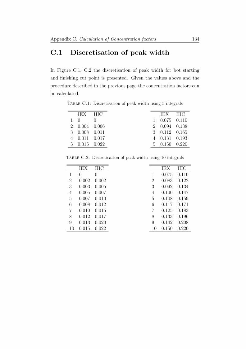
Appendix C. Calculation of Concentration factors 134
C.1 Discretisation of peak width
In Figure C.1, C.2 the discretisation of peak width for bot starting
and finishing cut point is presented. Given the values above and the
procedure described in the previous page the concentration factors can
be calculated.
Table C.1: Discretisation of peak width using 5 integrals
IEX HIC1 0 02 0.004 0.0063 0.008 0.0114 0.011 0.0175 0.015 0.022
IEX HIC1 0.075 0.1102 0.094 0.1383 0.112 0.1654 0.131 0.1935 0.150 0.220
Table C.2: Discretisation of peak width using 10 integrals
IEX HIC1 0 02 0.002 0.0023 0.003 0.0054 0.005 0.0075 0.007 0.0106 0.008 0.0127 0.010 0.0158 0.012 0.0179 0.013 0.02010 0.015 0.022
IEX HIC1 0.075 0.1102 0.083 0.1223 0.092 0.1344 0.100 0.1475 0.108 0.1596 0.117 0.1717 0.125 0.1838 0.133 0.1969 0.142 0.20810 0.150 0.220

Appendix D
Simulation results from
gPROMS
The following figures, show the simulation results from gPROMS. In
all cases the curve with the red colour is the target protein and the rest
are the contaminants. The x axis is the time in seconds and the y axis
is the concentration of each component p in g/l.
To obtain these figures we used the parameters presented in Table 6.2.
135
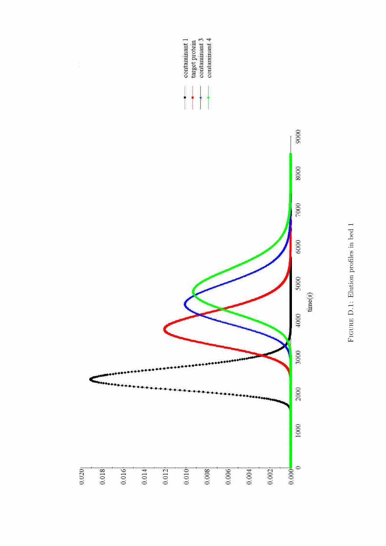
Appendix D. Simulation results from gproms 136
Fig
ure
D.1
:E
luti
onpr
ofile
sin
bed
1

Appendix D. Simulation results from gproms 137
Fig
ure
D.2
:E
luti
onpr
ofile
sin
bed
2

Appendix D. Simulation results from gproms 138
Fig
ure
D.3
:E
luti
onpr
ofile
sin
bed
3
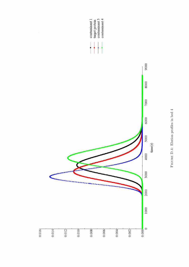
Appendix D. Simulation results from gproms 139
Fig
ure
D.4
:E
luti
onpr
ofile
sin
bed
4

Bibliography
[1] IMS Health. The global pharmaceurical market, 2011. URL
http://www.vfa.de/en/statistics/pharmaceuticalmarket/.
[2] E. Vasquez-Alvarez, M. E. Lienqueo, and J. M. Pinto. Opti-
mal synthesis of protein purification processes. Biotechnology
Progress, 17:685–696, 2001.
[3] E. M. Polykarpou, P. A. Dalby, and L. G. L. G. Papageorgiou. An
MINLP Formulation for the Synthesis of Chromatographic Pro-
tein Purification Processes with Product Loss. In European Sym-
posium on Computer Aided Process Engineering-19, volume 26 of
Computer-Aided Chemical Engineering, pages 1057–1062, 2009.
[4] G. Jagschies. Process-scale chromatography, 2000.
[5] G. Walsh. Biopharmaceutical benchmarks 2010. Nature biotech-
nology, 28(9):917 – 924, 2010.
[6] IMS Health. Ims health forecasts global pharmaceutical mar-
ket growth of 5-7 percent in 2011, 2010. URL http://www.
imshealth.com/portal/site/imshealth/.
[7] B. Munos. Lessons from 60 years of pharmaceutical innovation.
Nature Reviews Drug Discovery, 8:959–968, 2009.
[8] Steven J Projan, Davinder Gill, Zhijian Lu, and Steven H Her-
rmann. Small molecules for small minds? The case for biologic
pharmaceuticals. Expert Opinion on Biological Therapy, 4:1345–
1350, 2004.
140

Bibliography 141
[9] S. Ahuja. Handbook of BioSeparations. Academic Press, 2000.
[10] L. S. Ettre. Nomenclature for Chromatography. Pure and Applied
Chemistry, 65(4):819–872, 1993.
[11] Kirk-Othmer. Encyclopedia of Chemical Technology, volume 2.
John Wiley and Sons, Inc., 5th edition, 2007.
[12] H. M. McNair and J. M. Miller. Basic Gas Chromatography. John
Wiley and Sons, Inc., 1998.
[13] J. P. Martin and R. L. M. Synge. A new form of Chromatogram
employing two liquid phases 1. A theory of Chromatography 2.
Application to the micro-determination of the higher monoamino-
acids in proteins. Biochemical Journal, 35:1358–1368, 1941.
[14] A. T. James and J. P. Martin. Gas liquid partition chromatogra-
phy: the separation and micro-estimation of volatile fatty acids
from formic acid to dodecanoic acid. Biochemical Journal, 50:
679–690, 1952.
[15] R. P. W. Scott. Contemporary Liquid Chromatography. John
Wiley and Sons, Inc., 1976.
[16] P. A. Schweitzer. Handbook of Separation for Chemical Engineers.
McGraw-Hill, Inc., 1996.
[17] J. J. McKetta. Encyclopedia of Chemical Processing and Design,
volume 8. Marcel Dekker, Inc., 1976.
[18] J. M. Coulson and J. F. Richardson. Chemical Engineer-
ing Volume 2: Particle Technology and Separation Processes.
Butterworth-Heinemann, 4th edition, 1991.
[19] A. Tiselius. Displacement development in adsorption analysis.
Stockholm Almqvist Wiksell Berlin Natura, 16A(18):1–18, 1943.
[20] R. Freitag and J. Breier. Displacement chromatography in
biotechnological downstream processing. Journal of chromatog-
raphy A, 691:101 – 112, 1995.

Bibliography 142
[21] A. Jungbauer. Chromatographic media for bioseparation. Journal
of Chromatography A, 1065(1):3–12, 2005.
[22] Pall Corporation. Mixed-mode chromatography selection guide,
2011. URL http://www.pall.com/.
[23] S. H. Ngiam, D. G. Bracewell, Y. Zhou, and N. J. Titchener-
Hooker. Quantifying process tradeoffs in the operation of chro-
matographic sequences. Biotechnology Progress, 19(4):1315–1322,
2003.
[24] C. R. Lowe, A. R. Lowe, and G. Gupta. New developments in
affinity chromatography with potential application in the produc-
tion of biopharmaceuticals. Journal of Biochemical and Biophys-
ical methods, 49:561–574, 2001.
[25] J. Curling. Process chromatography: Five decades of innovation.
Biopharm International, 20:10–19, 2007.
[26] T. M. Przybycien, N. S. Pujar, and L. M Steele. Alternative
bioseparation operations: life beyond packed-bed chromatogra-
phy. Current Opinion in Biotechnology, 15:469–478, 2004.
[27] G. Larsson, S. B. Jorgensen, M. N. Pons, B. Sonnleitner, A. Ti-
jsterman, and N. J. Titchener-Hooker. Minireview: Biochemical
engineering science. Journal of Biotechnology, 59(1-2):3–9, 1997.
[28] J. Thommes and M. Etzel. Alternatives to chromatographic sep-
arations. Biotechnology Progress, 23(1):42–45, 2007.
[29] B. Kelley. Industrialization of mab production technology the
bioprocessing industry at a crossroads. mAbs, 1(5):443–452, 2009.
[30] D. Low, R. O’Leary, and N. S. Pujar. Future of antibody pu-
rification. Journal of Chromatography B, 848(1):48 – 63, 2007.
Polyclonal and Monoclonal Antibody Production, Purification,
Process and Product Analytics.

Bibliography 143
[31] J. A. Asenjo and B. A. Andrews. Challenges and trends in biosep-
arations. Journal of Chemical Technology and Biotechnology, 83
(2):117–120, 2008.
[32] B. K. Nfor, T. Ahamed, G. W. K. van Dedem, L. A. M. van der
Wielen, E. J. A. X. van de Sandt, M. H. M. Eppink, and M. Ot-
tens. Design strategies for integrated protein purification pro-
cesses: challenges, progress and outlook. Journal of Chemical
Technology and Biotechnology, 83(2):124–132, 2008.
[33] FDA. International Committee on Harmonization Q8: Pharma-
ceutical Development FDA, 2009.
[34] A. Jungbauer and O. Kaltenbrunner. Fundamental questions
in optimizing ion-exchange chromatography of proteins using
computer-aided process design. Biotechnology and Bioengineer-
ing, 52(2):223–236, 1996.
[35] A. Mahn, M. E. Lienqueo, and J. C. Salgado. Methods of calcu-
lating protein hydrophobicity and their application in developing
correlations to predict hydrophobic interaction chromatography
retention. Journal of Chromatography A, 1216(10):1838–1844,
2009.
[36] J. Bonnerjea, S. Oh, M. Hoare, and P. Dunnill. Protein purifica-
tion: The right step at the right time. Biotechnology, 4:954–958,
1986.
[37] J. C. Salgado, I. Rapaport, and J. A. Asenjo. Predicting the be-
haviour of proteins in hydrophobic interaction chromatography 2.
using a statistical description of their surface amino acid distri-
bution. Journal of Chromatography A, 1107:120–129, 2006.
[38] F. Dismer and J. Hubbuch. A novel approach to characterize the
binding orientation of lysozyme on ion-exchange resins. Journal
of Chromatography A, 1149(2):312 – 320, 2007.

Bibliography 144
[39] F. Dismer, M. Petzold, and J. Hubbuch. Effects of ionic strength
and mobile phase ph on the binding orientation of lysozyme on
different ion-exchange adsorbents. Journal of Chromatography
A, 1194(1):11–21, 2008. 27th International Symposium on the
Separation of Proteins, Peptides and Polynucleotides.
[40] F. Dismer and J. Hubbuch. 3d structure-based protein retention
prediction for ion-exchange chromatography. Journal of Chro-
matography A, 1217(8):1343–1353, 2010.
[41] D. Karlsson, N. Jakobsson, A. Axelsson, and B. Nilsson. Model-
based optimization of a preparative ion-exchange step for anti-
body purification. Journal of Chromatography A, 1055(1-2):29 –
39, 2004.
[42] H. Weiqiang, Z. Xiangmin, and H. Fengli. Analysis of the ideal
model for a single component in preparative gradient elution chro-
matography. Analytical Chemistry, 79(6):2507–2517, 2007.
[43] J. M. Mollerup, T. B. Hansen, Steffen Kidal, Lars Sejergaard, and
Arne Staby. Development, modelling, optimisation and scale-up
of chromatographic purification of a therapeutic protein. Fluid
Phase Equilibria, 261(1-2):133 – 139, 2007.
[44] S. Chan, N. Titchener-Hooker, D. G. Bracewell, and E. Sorensen.
A systematic approach for modeling chromatographic process-
esapplication to protein purification. AIChE Journal, 54(4):965–
977, 2008.
[45] C. Shene, A. Lucero, B. A. Andrews, and J. A. Asenjo. Math-
ematical modeling of elution curves for a protein mixture in ion
exchange chromatography and for the optimal selection of op-
erational conditions. Biotechnology and Bioengineering, 95(4):
704–713, 2006.
[46] O. Kaltenbrunner, O. Giaverini, D. Woehle, and J. A. Asenjo. Ap-
plication of chromatographic theory for process characterization
Bibliography 145
towards validation of an ion-exchange operation. Biotechnology
and Bioengineering, 98(1):201–210, 2007.
[47] H. K. Teoh, M. Turner, N. Titchener-Hooker, and E. Sorensen.
Experimental verification and optimisation of a detailed dynamic
high performance liquid chromatography column model. Com-
puters and Chemical Engineering, 25(4-6):893 – 903, 2001.
[48] C. A. Orellana, C. Shene, and J. A. Asenjo. Mathematical mod-
eling of elution curves for a protein mixture in ion exchange chro-
matography applied to high protein concentration. Biotechnology
and Bioengineering, 104(3):572–581, 2009.
[49] M. Degerman, N. Jakobsson, and B. Nilsson. Designing robust
preparative purification processes with high performance. Chem-
ical Engineering and Technology, 31(6), 2008.
[50] N. Jakobsson, M. Degerman, E. Stenborg, and B. Nilsson. Model
based robustness analysis of an ion-exchange chromatography
step. Journal of Chromatography A, 1138(1-2):109 – 119, 2007.
[51] S. H. Ngiam, Y. H. Zhou, M. K. Turner, and N. J. Titchener-
Hooker. Graphical method for the calculation of chromatographic
performance in representing the trade-off between purity and re-
covery. Journal of Chromatography A, 937(1-2):1–11, 2001.
[52] S. Edwards-Parton, N. F. Thornhill, D. G. Bracewell, J. M. Lid-
dell, and N. J. Titchener-Hooker. Principal component score mod-
eling for the rapid description of chromatographic separations.
Biotechnology Progress, 24(1):202–208, 2008.
[53] R. S. Salisbury, D. G Bracewell, and N. J. Titchener-Hooker. A
methodology for the graphical determination of operating condi-
tions of chromatographic sequences incorporating the trade-offs
between purity and yield. Journal of Chemical Technology and
Biotechnology, 81(11):1803–1813, 2006.

Bibliography 146
[54] C. B. Mazza, N. Sukumar, C. M. Breneman, and S. M. Cramer.
Prediction of protein retention in ion-exchange systems using
molecular descriptors obtained from crystal structure. Analyti-
cal Chemistry, 73(22):5457–5461, 2001.
[55] M. Song, C. M. Breneman, J. Bi, N. Sukumar, K. P. Bennett,
S. M. Cramer, and N. Tugcu. Prediction of protein retention
times in anion-exchange chromatography systems using support
vector regression. Journal of Chemical Information and Computer
Sciences, 42(6):1347–1357, 2002.
[56] A. Ladiwala, K. Rege, C. M. Breneman, and S. M. Cramer. Inves-
tigation of mobile phase salt type effects on protein retention and
selectivity in cation-exchange systems using quantitative struc-
ture retention relationship models. Langmuir, 19(20):8443–8454,
2003.
[57] A. Ladiwala, F. Xia, Q. Luo, C. M. Breneman, and S. M. Cramer.
Investigation of protein retention and selectivity in hic systems us-
ing quantitative structure retention relationship models. Biotech-
nology and Bioengineering, 93(5):836–850, 2006.
[58] J. Chen, T. Yang, Q. Luo, C. M. Breneman, and S. M. Cramer.
Investigation of protein retention in hydrophobic interaction chro-
matographic (hic) systems using the preferential interaction the-
ory and quantitative structure property relationship models. Re-
active and Functional Polymers, 67(12):1561–1569, 2007.
[59] J. Chen, T. Yang, and S. M. Cramer. Prediction of protein reten-
tion times in gradient hydrophobic interaction chromatographic
systems. Journal of Chromatography A, 1177(2):207–214, 2008.
[60] M. Wiendahl, P. S. Wierling, J. Nielsen, D. F. Christensen,
J. Krarup, A. Staby, and J. Hubbuch. High throughput screen-
ing for the design and optimization of chromatographic processes
miniaturization, automation and parallelization of breakthrough

Bibliography 147
and elution studies. Chemical Engineering and Technology, 31(6):
893–903, 2008.
[61] S. Chhatre and N. J. Titchener-Hooker. Review: Microscale
methods for high-throughput chromatography development in the
pharmaceutical industry. Journal of Chemical Technology and
Biotechnology, 84(7):927–940, 2009.
[62] A. Jungbauer. Insights into the chromatography of proteins pro-
vided by mathematical modeling. Current Opinion in Biotech-
nology, 7(2):210–218, 1996.
[63] C. Ostlund. Large-scale purification of monoclonal antibodies.
Trends Biotechnology, 4:288–293, 1986.
[64] J. A. Asenjo, L. Herrera, and B. Byrne. Development of an ex-
pert system for selection and synthesis of protein purification pro-
cesses. Journal of Biotechnology, 11:275–298, 1989.
[65] S. M. Wheelwright. The design of downstream processes for large-
scale protein purification. Journal of Biotechnology, 11:89–102,
1989.
[66] J. A. Asenjo. Selection of operations in separation processes.
Bioprocess Technology, 9:3–16, 1990.
[67] H. Eriksson, K. Sandahl, G. Forslund, and B. Gsterlund.
Knowledge-based planning for protein purification. Chemomet-
rics and Intelligent Laboratory Systems: Laboratory Information
Management, 13:173–184, 1991.
[68] E. W. Leser and J. A. Asenjo. Rational design of purification
processes for recombinant proteins. Journal of Chromatography
B: Biomedical Sciences and Applications, 584(1):43 – 57, 1992.
[69] E. Watanabe, S. Tsoka J. A., and Asenjo. Selection of chromato-
graphic protein purification operations based on physicochemical
propertiesa. Annals of the New York Academy of Sciences, 721
(1):348–364, 1994.

Bibliography 148
[70] E. W. Leser and J. A. Asenjo. The rational selection of purifi-
cation processes for proteins: An expert system for downstream
processing designa. Annals of the New York Academy of Sciences,
721(1):337–347, 1994.
[71] N. Nishida, G. Stephanopoulos, and A. W. Westerberg. A review
of process synthesis. AIChE Journal, 27:321–351, 1981.
[72] M. E. Lienqueo. Desarollo de un sistema experto para la selection
racional de processos de purification de proteinas:optimizacion de
criterios se seleccion de sequenciase. PhD thesis, Universidad De
Chile Facultad de Ciencias Fisicas y matematicas departamento
de Ingeniera Quimica, 1999.
[73] M. E. Lienqueo, E. W. Leser, and J. A. Asenjo. An expert system
for the selection and synthesis of multi-step protein separation
processes. Computers Chemical Engineering, 20:189–194, 1996.
[74] M. E. Lienqueo and J. A. Asenjo. Use of expert systems for
the synthesis of downstream protein processes. Computers and
Chemical Engineering, 24:2339–2350, 2000.
[75] J. A. Asenjo and B. A. Andrews. Is there a rational method to
purify proteins? from expert systems to proteomics. Journal of
Molecular Recognition, 17(3):236–247, 2004.
[76] M. A. Steffens, E. S. Fraga, and I. D. L. Bogle. Synthesis of
bioprocesses using physical propertie data. Biotechnology and
Bioengineering, 68(2):218–230, 1999.
[77] M. A. Steffens, E. S. Fraga, and I. D. L. Bogle. Synthesis of
purification tags for optimal downstream processing. Computers
and Chemical Engineering, 24:717–720, 2000.
[78] E. Vasquez-Alvarez and J. M. Pinto. Efficient milp formulation
for the optimal synthesis of chromatographic protein purification
processes. Journal of Biotechnology, 110:295–311, 2004.

Bibliography 149
[79] E. Simeonidis, J. M. Pinto, M. E. Lienqueo, S. Tsoka, and L. G.
Papageorgiou. Minlp models for the synthesis of optimal peptide
tags and downstream protein processing. Biotechnology Progress,
21:875–884, 2005.
[80] M. E. Lienqueo, J. C. Salgado, O. Giaverini, and J. A. Asenjo.
Computer-aided design to select optimal polypeptide tags to as-
sist the purification of recombinant proteins. Separation and Pu-
rification Technology, 65(1):86–94, 2009.
[81] J. M. Natali, J. M. Pinto, and L. G. Papageorgiou. Efficient milp
formulations for the simultaneous optimal peptide tag design and
downstream processing synthesis. AIChE Journal, 55:2303–2317,
2009.
[82] M. E. Lienqueo, J. C. Salgado, O. Giaverini, and J. A. Asenjo.
Computer-aided design to select optimal polypeptide tags to as-
sist the purification of recombinant proteins. Separation and Pu-
rification Technology, 65(1):86 – 94, 2009. Advances in Bioparti-
tioning and Purification.
[83] B. K. Nfor, P. D. E. M. Verhaert, L. A. M. van der Wielen,
J. Hubbuch, and M. Ottens. Rational and systematic protein
purification process development: the next generation. Trends in
Biotechnology, 27(12):673–679, 2009.
[84] E. Vasquez-Alvarez and J. M. Pinto. Mixed integer optimiza-
tion models for the Synthesis of Protein Purification Processes
with product loss. In European Symposium on Computer Aided
Process Engineering-12, volume 10 of Computer-Aided Chemical
Engineering, pages 373–378, 2002.
[85] E. Vasquez-Alvarez and J. M. Pinto. A mixed integer linear pro-
gramming model for the optimal synthesis of protein purification
processes with product loss. Chemical and Biochemical Engineer-
ing Quarterly, 17(1):77–84, 2003.

Bibliography 150
[86] N. J. Samsatli and N. Shah. Optimal integrated design of bio-
chemical processes. Computers and Chemical Engineering, 20(1):
310–320, 1996. European Symposium on Computer Aided Pro-
cess Engineering-6.
[87] N. J. Samsatli and N. Shah. An optimization based design pro-
cedure for biochemical processes: Part i: Preliminary design and
operation. Food and Bioproducts Processing, 74(4):221–231, 1996.
[88] N. J. Samsatli and N. Shah. An optimization based design proce-
dure for biochemical processes: Part ii: Detailed scheduling. Food
and Bioproducts Processing, 74(4):232–242, 1996.
[89] J. M. Montagna, A. R. Vecchietti, O. A. Iribarren, J. M. Pinto,
and J. A. Asenjo. Optimal design of protein production plants
with time and size factor process models. Biotechnology Progress,
16(2):228–237, 2000.
[90] J. A. Asenjo, J. M. Montagna, A. R. Vecchietti, O. A. Iribarren,
and J. M. Pinto. Strategies for the simultaneous optimization
of the structure and the process variables of a protein production
plant. Computers and Chemical Engineering, 24(9-10):2277–2290,
2000.
[91] J. M. Pinto, J. M. Montagna, A. R. Vecchietti, O. A. Iribarren,
and J. A. Asenjo. Process performance models in the optimization
of multiproduct protein production plants. Biotechnology and
Bioengineering, 74(6):451–465, 2001.
[92] J. A. Asenjo and B. A. Andrews. Protein purification using chro-
matography: selection of type, modelling and optimization of
operating conditions. Journal of Molecular Recognition, 22(2):
65–76, 2009.
[93] A. A. Shukla and J. Thommes. Recent advances in large-scale
production of monoclonal antibodies and related proteins. Trends
in Biotechnology, 28(5):253 – 261, 2010.

Bibliography 151
[94] M. E. Lienqueo, A. Mahn, and J. A. Asenjo. Mathematical cor-
relations for predicting protein retention times in hydrophobic
interaction chromatography. Journal of Chromatography A, 978
(1-2):71 – 79, 2002.
[95] A. Brooke, D. Kendrick, A. Meeraus, and Raman. GAMS - A
User’s Guide. GAMS Development Corporation, 2008.
[96] J. M. Natali and J. M. Pinto. Piecewise polynomial interpolations
and approximations of one-dimensional functions through mixed
integer linear programming. Optimization Methods & Software,
24:783–803, 2009.
[97] M. Tawarmalani and N. V. Sahinidis. A polyhedral branch-and-
cut approach to global optimization. Mathematical Programming,
103:225–249, 2005.
[98] A. Jungbauer and O. Kaltenbrunner. Fundamental questions
in optimizing ion-exchange chromatography of proteins using
computer-aided process design. Biotechnology and Bioengineer-
ing, 52(2):223–236, 1996.
[99] G. Guiochon. Preparative liquid chromatography. Journal of
Chromatography A, 965(1-2):129 – 161, 2002.
[100] G. Guiochon and S. G. Shirazi. Fundamentals of Preparative and
Nonlinear Chromatography. Academic Press, Boston, 4th edition,
1994.
[101] F. Gritti and G. Guiochon. The ultimate band compression factor
in gradient elution chromatography. Journal of Chromatography
A, 1178(1-2):79 – 91, 2008.
[102] E. Vasquez-Alvarez and J. M. Pinto. Dynamic liquid chromatog-
raphy column models in protein separation processes. In 4th
Mercosur Congress on Process Systems Engineering, pages 1–10,
2005.

Bibliography 152
[103] M. Almqvist. Modeling and calibration of preparative chromatog-
raphy in gproms separations of protein monomers from dimers,
2009.
[104] J. C. Bellot and J. S. Condoret. Modelling of liquid chromatog-
raphy equilibria. Process Biochemistry, 28(6):365 – 376, 1993.
[105] J. C. Bellot and J. S. Condoret. Liquid chromatography mod-
elling: a review. Process Biochemistry, 26(6):363 – 376, 1991.
[106] Process Systems Enterprise. gproms, 1997-2001. URL http:
//www.psenterprise.com/gproms.

List of Communications
1. Eleftheria M. Polykarpou, Paul Dalby, Lazaros G. Papageorgiou
Optimisation of Chromatography for the purification of Mutant
Proteins, IMRC Meeting 2009, London, UK (05/2009)
2. Eleftheria M. Polykarpou, Paul Dalby, Lazaros G. Papageorgiou
An MINLP Formulation for the Synthesis of Chromatographic
Protein Purification Processes with Product Loss
Computer Aided Chemical Engineering, ESCAPE19, Volume
26, 2009, Pages 1057-1062
3. Eleftheria M. Polykarpou, Paul Dalby, Lazaros G. Papageorgiou
Synthesis of chromatographic protein purification processes us-
ing optimisation techniques, EURO XXIV, Lisbon, Portugal
(06/2010)
4. Eleftheria M. Polykarpou, Paul Dalby, Lazaros G. Papageorgiou
Synthesis of Downstream Processes: Optimal selection of Chro-
matographic Sequences, Recovery of Biological Products XIV,
Lake Tahoe, CA, USA (08/2010)
5. Eleftheria M. Polykarpou, Paul Dalby, Lazaros G. Papageorgiou
Synthesis of Downstream Processes: Optimal Selection of Chro-
matographic Sequences, CPSE Consortium, London, UK (12/2010)
6. Eleftheria M. Polykarpou, Paul Dalby, Lazaros G. Papageorgiou
Optimal Synthesis of Chromatographic Trains for Downstream
Protein Processing, Biotechnology Progress Journal (Accepted)
153
Bibliography 154
7. Eleftheria M. Polykarpou, Paul Dalby, Lazaros G. Papageorgiou
An MILP formulation for the synthesis of protein purification pro-
cesses, Chemical Engineering Research and Design Jour-
nal (Under review)
8. Eleftheria M. Polykarpou, Paul Dalby, Lazaros G. Papageorgiou
Novel efficient optimisation systems for purification process syn-
thesis, Biochemical Engineering Journal (Under review)