Optimal Traffic Sharing in GERAN

Salvador Luna-Ramırez, Matıas Toril, Mariano Fernandez-Navarro∗and Volker Wille†

October 15, 2009

Abstract

In a mobile communications network, the uneven spatial distribution of traffic demand canbe dealt with by redefining cell service areas. When resizing cells, network operators often aimat equalizing call blocking rates throughout the network in the hope that this will maximizethe total carried traffic in the network. In this paper, an analytical teletraffic model for thetraffic sharing problem in GSM-EDGE Radio Access Network (GERAN) is presented. Fromthis model, a closed-form expression is derived for the optimal traffic sharing criterion betweencells. Using this expression, it can be shown that balancing call blocking rate between adjacentcells is not the optimal strategy. Results show that using the optimal traffic sharing criterioninstead of balancing blocking rates across the network can increase network capacity, evenunder restrictions in the cell resizing process.

1 Introduction

In recent years, the success of mobile communication services has led to an exponential increase oftraffic in cellular networks. Thus, traffic engineering has become one of the main areas of interestfor cellular network operators. For circuit-switched traffic, the availability of well-established trafficmodels allows proper dimensioning of traffic resources during network design. However, as networkevolves, the matching between the spatial distribution of traffic demand and network resourcesbecomes poorer. Therefore, continuous adaptation of network resources is needed. As capitalexpenditures are limited, the addition of new resources is kept to a minimum. In this situation,traffic management remains the only solution to keep network performance within pre-specifiedlevels.

Managing circuit-switched traffic in a cellular network mainly consists of selecting the base sta-tion to which every mobile station is attached. In GSM-EDGE Radio Access Network (GERAN),this is performed by three Radio Resource Management (RRM) procedures: cell re-selection, calladmission control and handover, [1]. Fast traffic fluctuations are dealt with by advanced RRMfeatures, such as dynamic load sharing, [2], and dynamic half-rate coding, [3]. However, these pro-cedures are unable to solve localized congestion problems caused by spatial concentration of trafficdemand, as shown in [4]. In the long term, these problems are solved by re-planning strategies,such as the extension of transceivers or cell splitting. However, in the short term, the adaptationof cell service areas is the only solution for cells that cannot be upgraded quickly. Cell resizingis performed by modifying base station transmit power, [5], antenna uptilting/downtilting, [6], oradjusting RRM parameter settings, [7][8][9]. Before applying these techniques, the operator has todefine the desired traffic share between network cells, for which an analytical network model canbe used.

Several analytical teletraffic models have been proposed in the literature for Time-FrequencyDivision Multiple Access (TDMA/FDMA) cellular networks. Hong and Rappaport, [10], proposed

∗This and previous authors are on the staff of Communications Engineering Dept., University of Malaga, Malaga,Spain, {sluna,mtoril,mariano}@ic.uma.es

†Performance Services, Nokia Siemens Networks, Huntingdon, UK, volker.wille@nsn.com

1

their classical Markov chain model with Poisson fresh call and handover arrivals and exponentialservice times to evaluate the performance of prioritizing and queueing handover requests. Guerin,[11], extended the model to consider queueing of both fresh call and handover requests. Laterstudies improved the model by considering more general distributions of channel holding time,[12][13][14], correlated arrivals, [15][16], retrials, [17][18], multiple services, [19][20][21], and multiplenetwork layers, [22][23]. These models have been extended to other radio access technologies,namely Code Division Multiple Access (CDMA), [24][25], and Orthogonal Frequency DivisionMultiple Access (OFDMA), [26].

Most of the previous references use queueing models to evaluate the performance of novelRRM algorithms. However, only a few references use these models to find an optimal networkparameter configuration for re-planning purposes, [27][28][29][30][31]. In [27], the design of a multi-tier network is solved as an optimization problem, whose goal is to minimize total system cost andthe decision variables are the cell sizes and the number of channels per tier. In [28], the minimumnumber of channels per traffic class in a channel reservation scheme is obtained based on ananalytical model of a multi-service scenario. More related to this paper, [29] and [30] formulate thetraffic sharing between adjacent cells as a classical optimization problem. In their approach, thegoal is to minimize call blocking in the network and the decision variables are the handover margins,defined on a per-adjacency basis. For this purpose, the spatial traffic distribution is estimatedfrom measurement reports and mobile positioning data, respectively. In [31], an analytical modelof WCDMA cell capacity is used to minimize the total downlink interference in a real scenario bytuning sector azimuths and antenna tilts. However, none of these references propose a closed-formexpression of the optimal solution for the traffic sharing problem. Thus, in these studies, the bestsolution is found by heuristic search methods, without any proof of optimality.

In this paper, a novel method for determining the best traffic share between cells in a GERANsystem is presented. The proposed method computes the optimal spatial distribution of traffic,given a certain distribution of network resources. The main decision variables are the trafficdemand originated by fresh calls and handovers in each cell. Two queueing models are presented,corresponding to the cases when traffic is reallocated by tuning parameters in the call admissioncontrol or the handover algorithm. For both models, a closed-form expression of the optimal trafficsharing criterion is derived based on the properties of the Erlang-B formula. The analysis showsthat the common rule of balancing call blocking rates between adjacent cells is not the optimalstrategy. Performance assessment is carried out in a set of realistic test cases. During the tests, theproposed exact method is compared with approaches currently used by network operators. Themain contribution of this paper is a novel criterion for balancing circuit-switched traffic betweenadjacent cells, which can easily be integrated in automatic network optimization tools.

The rest of the paper is organized as follows. Section 2 formulates the traffic sharing problemin the two network models considered, Section 3 presents the performance of several traffic sharingcriteria in different scenarios and Section 4 presents the main conclusions of the study.

2 Problem Formulation

This section outlines the problem of determining the optimal spatial traffic distribution when re-planning an existing TDMA/FDMA cellular network. For this purpose, two different networkmodels are presented. A first naive model considers the case of re-distributing traffic demand bytuning parameters in the call admission control algorithm. Then, a more refined model considersthe more realistic case of re-distributing traffic by tuning handover parameters under constraintson the traffic re-allocation process.

2.1 Naive Model

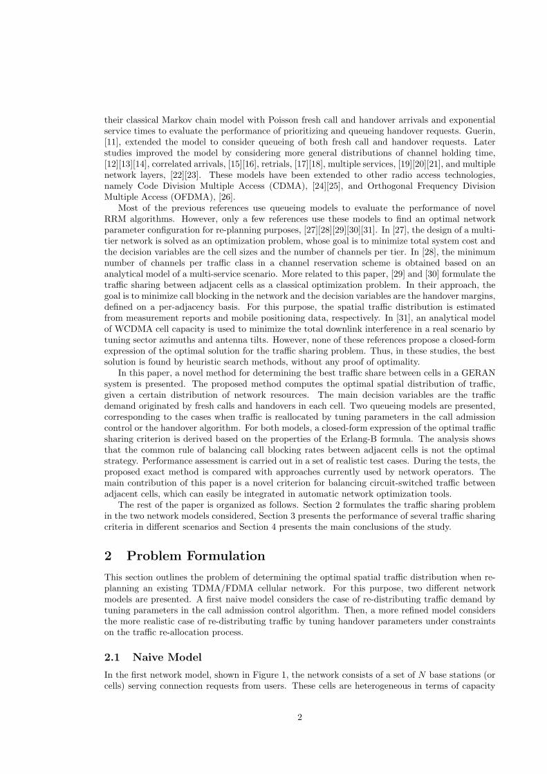
In the first network model, shown in Figure 1, the network consists of a set of N base stations (orcells) serving connection requests from users. These cells are heterogeneous in terms of capacity

2

1 1( , )E cµλ2 2( , )E cµλ( , )N NE cµλ

1 1( , )N NE cλµ

−−

11 ( , )N i ibT iA E cµ µλ λ

=

= ⋅∑Figure 1: A naive model of the traffic sharing problem.

(i.e., each cell i has a different number of channels, ci). User demand is modeled by a unique flow ofcalls that can be freely distributed among cells (i.e., full overlapping between all cells is assumed).The call arrival process is a time-invariant Poisson process with overall rate λT . The service timeis an exponentially distributed random variable with parameter µ = 1/MCD, where MCD is themean call duration. Thus, the total offered traffic in the network is AT = λT /µ = λT ·MCD. Theassignment of a user to a cell is performed during connection set-up by the Call Admission Control(CAC) algorithm and maintained throughout the call. Since there is no possibility of handlingover a call between cells, the channel holding time in a cell coincides with the call duration, andthe service rate per channel is identical in all network cells, i.e., µi = µ = 1/MCD. Finally, it isassumed that a call attempt is lost if all channels in the cell are busy.

Most of the previous assumptions are widely used in the literature. The considered call arrivaland holding time distributions are standard for voice traffic in telecommunication systems, whetherfixed, [32], or mobile, [33]. The loss assumption is applicable to systems with access control andwithout queueing or retrials (e.g., [10][25][26]). The permanent association of the mobile to thecell where the call is initiated, equivalent to not modeling user mobility, has also been used inmany studies (e.g., [33][34]). Such an assumption is reasonable if cell size is large compared to thedistance traveled by the user during the call. More debatable is the condition of full overlappingbetween cells, as will be discussed later.

Under these assumptions, the call blocking probability in a cell is given by the Erlang-B formula

E(Ai, ci) =

Aici

ci!ci∑

j=1

Aij

j!

, (1)

where Ai and ci are the offered traffic and the number of channels in cell i, respectively. The totalblocked traffic in the network is the sum of blocked traffic in each cell, computed as

AbT =N∑i=1

Abi =N∑i=1

Ai E(Ai, ci) . (2)

In this work, the decision of assigning a connection to a cell does not depend on the currentstate of the system (as in RRM), but it is taken during the planning stage by defining cell serviceareas. Hence, the goal of traffic sharing is to find the best partitioning of traffic demand amongcells so that the total blocked traffic is minimized. The underlying optimization problem can beformulated as

3

Minimize

N∑i=1

Ai E(Ai, ci) (3)

subject to

N∑i=1

Ai = AT , (4)

Ai ≥ 0 ∀ i = 1 : N . (5)

This formulation ensures a minimum total blocked traffic, given that the total offered traffic in thenetwork is AT and all offered traffic values in cells are non-negative.

In the Appendix, it is shown that the solution to (3)-(5) is the one satisfying that

E(Ai, ci) +Ai∂E(Ai, ci)

∂Ai= E(Aj , cj) +Aj

∂E(Aj , cj)

∂Aj∀ i, j = 1 : N . (6)

The previous equation shows that the total blocked traffic is minimized when the indicatorE(Ai, ci)+

Ai · ∂E(Ai,ci)∂Ai

is the same for all cells. Such an indicator, hereafter referred to as incremental blockingprobability, adds a term to the blocking probability, E(Ai, ci). This conclusion seems contrary tothe common practice of equalizing network blocking throughout the network. In a homogeneousnetwork, all cells have the same number of channels (i.e., ci = cj) and, for symmetry reasons, (6)has a trivial solution Ai = Aj . In these conditions, equalizing any traffic indicator leads to theoptimal solution. However, when cells have different capacity, it is proved in the appendix thatbalancing blocking probabilities (i.e., first term on both sides of (6)) does not lead to the optimalsolution.

An intuitive interpretation of the incremental blocking probability, IBP , can be given by usingthat, [35],

∂E(Ai, ci)

∂Ai= E(Ai, ci)

[ciAi

− 1 + E(Ai, ci)

]. (7)

Thus,

IBP (Ai, ci) = E(Ai, ci) +AiE(Ai, ci)

[ciAi

− 1 + E(Ai, ci)

](8)

= E(Ai, ci) [1 + ci −Ai(1− E(Ai, ci))] .

By noting that {ci−Ai(1−E(Ai, ci))} is the average number of free channels in a cell with offeredtraffic Ai and ci channels, Nfc(Ai, ci), (8) is re-written as

IBP (Ai, ci) = E(Ai, ci) [1 +Nfc(Ai, ci)] . (9)

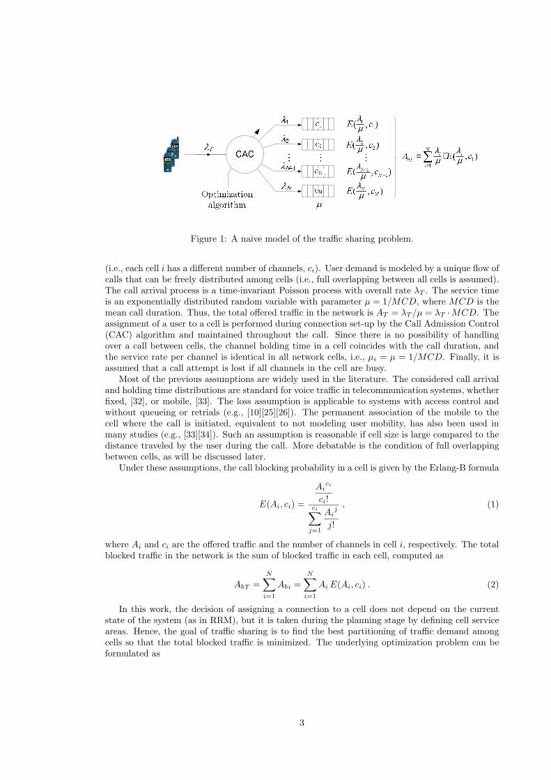
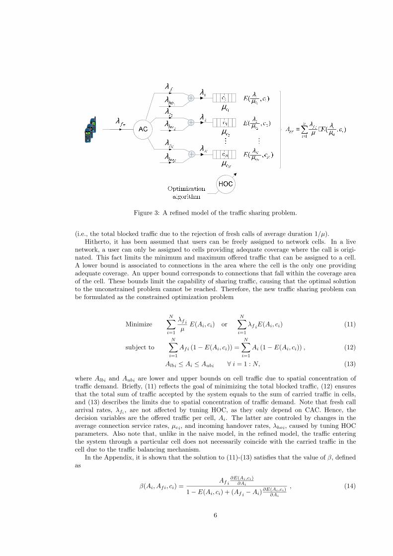
Figure 2 shows the incremental blocking probability in a cell with increasing offered traffic fordifferent number of channels. It is observed that the incremental blocking probability is a non-decreasing function of the offered traffic. Thus, it is clear that, in cells with a different numberof channels, the same value of incremental blocking indicator is reached with different values ofoffered traffic. It should be pointed out that the values of ci in the figure reflect the number oftraffic channels (i.e., time slots) in a cell with 1, 2, 3 and 4 transceivers in a live GERAN network.

2.2 Refined Model

The naive model assumes that: a) users can be freely assigned to cells in the network, b) theassignment of users to cells is performed during call set-up and not modified later, and c) allcells can provide adequate coverage during the entire call. Under these assumptions, the desired

4

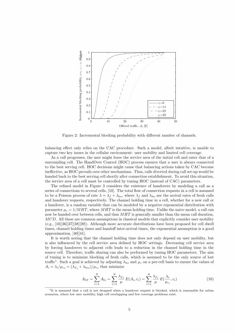
Figure 2: Incremental blocking probability with different number of channels.

balancing effect only relies on the CAC procedure. Such a model, albeit intuitive, is unable tocapture two key issues in the cellular environment: user mobility and limited cell coverage.

As a call progresses, the user might leave the service area of the initial cell and enter that of asurrounding cell. The HandOver Control (HOC) process ensures that a user is always connectedto the best serving cell. HOC decisions might cause that balancing actions taken by CAC becomeineffective, as HOC prevails over other mechanisms. Thus, calls diverted during call set-up would behanded back to the best serving cell shortly after connection establishment. To avoid this situation,the service area of a cell must be controlled by tuning HOC (instead of CAC) parameters.

The refined model in Figure 3 considers the existence of handovers by modeling a call as aseries of connections to several cells, [10]. The total flow of connection requests in a cell is assumedto be a Poisson process of rate λ = λf + λho, where λf and λho are the arrival rates of fresh callsand handover requests, respectively. The channel holding time in a cell, whether for a new call ora handover, is a random variable that can be modeled by a negative exponential distribution withparameter µc = 1/MHT , where MHT is the mean holding time. Unlike the naive model, a call cannow be handed over between cells, and thus MHT is generally smaller than the mean call duration,MCD. All these are common assumptions in classical models that explicitly consider user mobility(e.g., [10][36][37][38][39]). Although more accurate distributions have been proposed for cell dwelltimes, channel holding times and handoff inter-arrival times, the exponential assumption is a goodapproximation, [40][41].

It is worth noting that the channel holding time does not only depend on user mobility, butis also influenced by the cell service area defined by HOC settings. Decreasing cell service areaby forcing handovers to adjacent cells leads to a reduction in the channel holding time in thesource cell. Therefore, traffic sharing can also be performed by tuning HOC parameters. The aimof tuning is to minimize blocking of fresh calls, which is assumed to be the only source of losttraffic1. Such a goal is achieved by adjusting λho and µc on a per-cell basis to ensure the values ofAi = λi/µci = (λf i + λhoi)/µci that minimize

AbT =N∑i=1

Abi =N∑i=1

λf i

µE(Ai, ci) =

N∑i=1

λf i

µE(

λi

µci

, ci) (10)

1It is assumed that a call is not dropped when a handover request is blocked, which is reasonable for urbanscenarios, where low user mobility, high cell overlapping and few coverage problems exist.

5

1 11( , )cE cµλ 1 ( , )icN f i ib iT iA E cµµ

λ λ=

= ⋅∑1fλ 2fλ fNλ

2hoλ

1hoλ Nhoλ

1λ 2λ Nλ

Tfλ1cµ 2cµ Ncµ

2 22( , )cE cµλ( , )N NNcE cµλ

Figure 3: A refined model of the traffic sharing problem.

(i.e., the total blocked traffic due to the rejection of fresh calls of average duration 1/µ).Hitherto, it has been assumed that users can be freely assigned to network cells. In a live

network, a user can only be assigned to cells providing adequate coverage where the call is origi-nated. This fact limits the minimum and maximum offered traffic that can be assigned to a cell.A lower bound is associated to connections in the area where the cell is the only one providingadequate coverage. An upper bound corresponds to connections that fall within the coverage areaof the cell. These bounds limit the capability of sharing traffic, causing that the optimal solutionto the unconstrained problem cannot be reached. Therefore, the new traffic sharing problem canbe formulated as the constrained optimization problem

Minimize

N∑i=1

λf i

µE(Ai, ci) or

N∑i=1

λf iE(Ai, ci) (11)

subject to

N∑i=1

Afi (1− E(Ai, ci)) =

N∑i=1

Ai (1− E(Ai, ci)) , (12)

Albi ≤ Ai ≤ Aubi ∀ i = 1 : N, (13)

where Albi and Aubi are lower and upper bounds on cell traffic due to spatial concentration oftraffic demand. Briefly, (11) reflects the goal of minimizing the total blocked traffic, (12) ensuresthat the total sum of traffic accepted by the system equals to the sum of carried traffic in cells,and (13) describes the limits due to spatial concentration of traffic demand. Note that fresh callarrival rates, λfi , are not affected by tuning HOC, as they only depend on CAC. Hence, thedecision variables are the offered traffic per cell, Ai. The latter are controled by changes in theaverage connection service rates, µci, and incoming handover rates, λhoi, caused by tuning HOCparameters. Also note that, unlike in the naive model, in the refined model, the traffic enteringthe system through a particular cell does not necessarily coincide with the carried traffic in thecell due to the traffic balancing mechanism.

In the Appendix, it is shown that the solution to (11)-(13) satisfies that the value of β, definedas

β(Ai, Afi, ci) =Af i

∂E(Ai,ci)∂Ai

1− E(Ai, ci) + (Af i −Ai)∂E(Ai,ci)

∂Ai

, (14)

6

is the same ∀ i. More precisely, the optimal solution is the one satisfying that

β(Ai, Afi, ci) = β(Aj , Afj , cj) , (15)

for all cells i, j where constraint (13) is inactive2, and

β(Au, Afu, cu)|Au=Aub≤ β(Ai, Afi, ci) ≤ β(Al, Afl, cl)|Al=Alb

(16)

for all cells l and u where constraint (13) is active due to the lower or upper bound, respectively.Basically, (15) shows that, in the absence of traffic constraints, the best performance in the refinedmodel is achieved by equalizing the indicator β across the network. Likewise, (16) suggests that, inthose cells where one of the traffic bounds is reached, traffic has to be fixed to the limit value andthe traffic excess (or defect) must be re-distributed among the remaining cells. This fact justifiesthat sharing the traffic between adjacent cells leads to the optimal solution even in the presenceof constraints on the offered traffic per cell.

3 Performance Analysis

In the previous section, the optimal traffic sharing criteria for two teletraffic models of a cellularnetwork have been presented. The following experiments quantify the benefit of the exact approachwhen compared to current heuristic approaches. For clarity, the analysis set-up is first introducedand results are then presented.

3.1 Analysis Set-up

Assessment is carried out over four test scenarios of increasing complexity. The first three scenariosconsist of 3 GERAN cells of uneven capacity. In the example, the number of channels per cell is29, 6 and 6, corresponding to 4, 1 and 1 transceivers, respectively. Scenario 1 considers the naivemodel, i.e., static users, full cell overlapping and, consequently, no constraints on traffic sharing.Scenario 2 considers the refined model with no constraints on traffic sharing, where user mobilityis taken into account, but full cell overlapping is still assumed (i.e., Albi=0, Aubi=∞). Thus, theimpact of user mobility can be quantified. Scenario 3 considers the refined model with limits tothe offered traffic in cells to evaluate the impact of limited cell coverage and spatial concentrationof traffic demand. Scenario 4 extends the analysis to a real case built from data taken from a livenetwork. This scenario corresponds to the cells served by a real base station controller. Unlikeprevious scenarios, cell traffic bounds, Albi and Aubi , are computed on a cell-by-cell basis fromgeometric considerations, as will be explained later.

Four traffic sharing strategies are tested. All methods aim to equalize some performance in-dicator across the network, differing in the particular indicator balanced. The first three are

heuristic methods that equalize the average traffic load, Li =Ai(1−E(Ai,ci))

ci, the blocking proba-

bility, E(Ai, ci), or the blocked traffic, AfiE(Ai, ci), respectively. These methods are hereafterreferred to as Load Balancing (LB), Blocking Probability Balancing (BPB) and Blocked TrafficBalancing (BTB), respectively. While LB is used by most traffic balancing algorithms for real-time purposes, [42][43], BPB is often used by network operators when optimizing their networks,[4][9]. The fourth method, referred to as Optimal Balancing (OB), considers the optimal sharingcriterion in each model (i.e., (6) for the naive model and (15)-(16) for the refined model).

To evaluate performance, the traffic share among cells is computed for each strategy. Foroptimal sharing (i.e., OB), this is performed by solving (3)-(5) and (11)-(13) analytically. Forheuristic strategies (i.e., LB, BPB and BTB), the balancing problem is formulated as the non-linear least squares problem

2An inequality constraint is inactive (or not binding) when the equality does not hold.

7

MinimizeN−1∑i=1

(I (Ai, ci)− I (Ai+1, ci+1))2 (17)

subject toN∑i=1

Ai = AT , (18)

for the naive model and

Minimize

N−1∑i=1

(I (Ai, ci)− I (Ai+1, ci+1))2 (19)

subject to

N∑i=1

Afi(1− E(Ai, ci)) =

N∑i=1

Ai(1− E(Ai, ci)) , (20)

Albi ≤ Ai ≤ Aubi ∀ i = 1 : N, (21)

for the refined model, where I(Ai, ci) is the value of the balanced indicator (i.e., average traffic load,blocking probability or blocked traffic) in cell i, expressed as a function of Ai and ci. Optimizationmodels are solved by the fsolve and fmincon functions in MATLAB Optimization Toolbox, [44].When possible, the Jacobian matrix is provided to the scripts to speed up computations. Duringassessment, the total blocked traffic, AbT , and the overall blocking rate, AbT

AT, are the main figures

of merit. A measure of network capacity for each strategy is computed as the total offered trafficin the scenario for an overall blocking probability of 2%. To quantify the loss of network capacityfor not implementing optimal sharing, traffic values are normalized by that of OB to give a relativecapacity figure

Cm =AT |GoS=2%, m

AT |GoS=2%, OB

, (22)

where AT |GoS=2%, m is the network capacity obtained by method m for a Grade of Service (GOS)of 2%. Finally, to quantify the impact of constraints on traffic sharing, capacity values in theconstrained case are normalized by that of OB in the unconstrained case, as

Cm,const =AT |GoS=2%, m, const

AT |GoS=2%, OB, unconst

, (23)

where AT |GoS=2%,m,const is the network capacity obtained by method m with constraints on theoffered traffic per cell.

3.2 Analysis Results

3.2.1 Scenario 1: Naive model

The first scenario considers the naive model with 3 cells of uneven capacity. The first experimentevaluates the performance of traffic sharing strategies for a fixed value of total offered traffic.Specifically, AT=30E(rlang), which leads to an overall offered traffic load ρ = AT

c1+c2+c3= 30

29+6+6 =0.73. Table 1 presents the results of the different strategies in separate columns. Each row in thetable presents the value of a teletraffic indicator. From top to bottom, the rows show total offeredtraffic (AT ), offered traffic (A), average traffic load (L), blocking probability (E), blocked traffic(A ·E), incremental blocking probability (E+A · ∇E) and total blocked traffic (AbT ). Indicatorsin bold are represented by vectors with the values in the three cells. Obviously, the second andthird components in every vector have the same value, as those cells have the same capacity in this

8

Method LB BPB BTB OB

[Balancing Criterion] [Li] [E(Ai, ci)] [Ai · E(Ai, ci)] [E(Ai, ci)+Ai∂E(Ai,ci)

∂Ai]

AT [E] 30

A [E] [19.88 5.06 5.06] [24 3 3] [21.64 4.18 4.18] [23 3.50 3.50]

L [0.67 0.67 0.67] [0.78 0.47 0.47 ] [0.73 0.61 0.61] [0.76 0.54 0.54]

E [%] [1.21 19.61 19.61] [5.22 5.22 5.22] [2.52 13.03 13.03] [3.95 8.24 8.24]

A ·E [E] [0.24 0.99 0,99] [1.25 0.16 0,16] [0.54 0.54 0.54] [0.91 0.29 0.29]

E+A · ∇E [0.13 0.58 0.58 ] [0.38 0.22 0.22 ] [0.22 0.44 0.44] [0.31 0.31 0.31]

AbT [E] 2.224 1.567 1.634 1.486

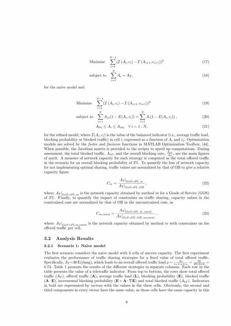
Table 1: Results of traffic sharing strategies in Scenario 1.

Figure 4: Overall blocking rate for different traffic sharing strategies in Scenario 1.

scenario (i.e., c2 = c3 = 6). Likewise, all three cells show the same value of the indicator equalizedin each strategy (i.e., L in LB, E in BPB, A ·E in BTB and E+A · ∇E in OB). For clarity, thesecases are highlighted in grey.

From the table, it is clear that the minimum total blocked traffic (i.e., AbT , last row) is obtainedby equalizing the incremental blocking probability (i.e., OB method, last column). Nonetheless, itis observed that large imbalances of the latter indicator still give adequate blocking performance.For instance, the BPB method (3rd column) causes that the incremental blocking probability (7th

row) in cells 2 and 3 is 43% smaller than in cell 1, i.e., [0.38 0.22 0.22]. Despite this imbalance,AbT only increases by 5.5% compared to the optimal strategy, i.e., 1.567 versus 1.486. In contrast,a 50% increase of blocked traffic is obtained by equalizing the average traffic load, i.e., 2.224 versus1.486. It is worth mentioning that, unexpectedly, equalizing the blocked traffic in cells is worsethan equalizing the blocking probability in terms of total blocked traffic.

The previous conclusions are valid, regardless of the total offered traffic, AT . Figure 4 showsthe evolution of the overall blocking rate with total offered traffic for all strategies. As expected,OB obtains the minimum blocked traffic (and, consequently, the maximum carried traffic) for allvalues of traffic demand. BPB and BTB achieve nearly the same blocking as OB, whereas LBperforms much worse.

From Figure 4, the total offered traffic for an overall blocking rate of 2% in each strategycan easily be found. This value is used as a measure of network capacity. Analysis shows that,in this scenario, the network capacity of BTB, BPB and LB relative to OB is CBTB = 0.99,

9

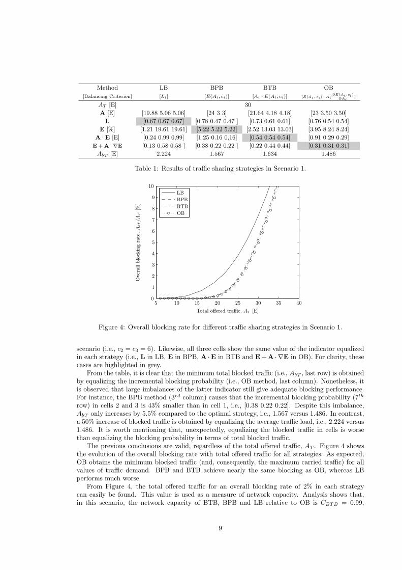
Figure 5: Overall blocking rate for different traffic sharing strategies in Scenario 2.

CBPB = 0.98 and CLB = 0.81, respectively. These results confirm that, in the naive model, BTBand BPB give near-optimal performance, while LB performs much worse. A closer analysis showsthat the gradient of the objective function in (3) in the direction imposed by constraint (4) is smallnear the optimum. Thus, significant changes in the traffic distribution cause limited performancedifferences.

3.2.2 Scenario 2: Refined model, unconstrained solution

The second scenario considers the refined model, where HOC can freely control the offered trafficdemand to each cell, Ai, given that the fresh call arrival rate in each cell, λfi , is fixed. Forsimplicity, a uniform spatial user distribution is assumed, i.e., λfi = λT /N .

Figure 5 shows the overall blocking rate of the different strategies with increasing offered trafficin the new scenario. In the figure, it is observed that BPB is still the best heuristic method, whileLB still performs the worst. More importantly, larger performance differences are now observedbetween methods. Specifically, the relative network capacity for BPB, BTB and LB is now 0.967,0.967 and 0.65, respectively. In other words, the improvement of network capacity achieved by OBis 3.3% compared to the best heuristic method. It can be concluded that, in the refined model, thebenefit of the exact approach becomes slightly more evident. Note that, under the assumption ofuniform spatial distribution (i.e., Af i = Af j), BPB and BTB lead to the same solution, since their

balance conditions (i.e., E(Ai, ci) = E(Aj , cj) and AfiE(Ai, ci) = AfjE(Aj , cj), respectively) areequivalent.

3.2.3 Scenario 3: Refined model, constrained solution

In previous scenarios, it has been assumed that the optimal traffic share can always be reachedby tuning HOC parameters. However, this is not true in live networks, where not all users canbe handed over to all cells. To account for this limitation, in the third scenario, lower and upperbounds, Albi and Aubi, are included on the offered traffic in cells. Such constraints reduce thefeasible solution space, causing that the optimal solution to the unconstrained problem might notbe reached.

To evaluate the impact of constraints on methods, bounds are gradually relaxed in the scenario.For clarity, bounds for all cells are controlled by a single parameter, ∆, referred to as deviationparameter, as

10

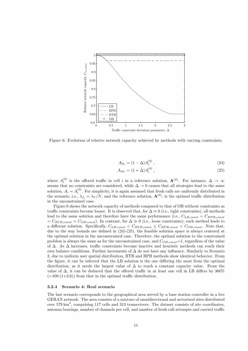
Figure 6: Evolution of relative network capacity achieved by methods with varying constraints.

Albi = (1−∆)A(0)i , (24)

Aubi = (1 +∆)A(0)i , (25)

where A(0)i is the offered traffic in cell i in a reference solution, A(0). For instance, ∆ → ∞

means that no constraints are considered, while ∆ → 0 causes that all strategies lead to the same

solution, Ai = A(0)i . For simplicity, it is again assumed that fresh calls are uniformly distributed in

the scenario, i.e., λfi = λT /N , and the reference solution, A(0), is the optimal traffic distributionin the unconstrained case.

Figure 6 shows the network capacity of methods compared to that of OB without constraints astraffic constraints become looser. It is observed that, for ∆ ≈ 0 (i.e., tight constraints), all methodslead to the same solution and therefore have the same performance (i.e., CLB,const = CBPB,const

= CBTB,const = COB,const). In contrast, for ∆ ≫ 0 (i.e., loose constraints), each method leads toa different solution. Specifically, CLB,const < CBTB,const ≤ CBPB,const < COB,const. Note that,due to the way bounds are defined in (24)-(25), the feasible solution space is always centered atthe optimal solution in the unconstrained case. Therefore, the optimal solution to the constrainedproblem is always the same as for the unconstrained case, and COB,const=1, regardless of the valueof ∆. As ∆ increases, traffic constraints become inactive and heuristic methods can reach theirown balance conditions. Further increments of ∆ do not have any influence. Similarly to Scenario2, due to uniform user spatial distribution, BTB and BPB methods show identical behavior. Fromthe figure, it can be inferred that the LB solution is the one differing the most from the optimaldistribution, as it needs the largest value of ∆ to reach a constant capacity value. From thevalue of ∆, it can be deduced that the offered traffic in at least one cell in LB differs by 360%(=100·(1+2.6)) from that in the optimal traffic distribution.

3.2.4 Scenario 4: Real scenario

The last scenario corresponds to the geographical area served by a base station controller in a liveGERAN network. The area consists of a mixture of omnidirectional and sectorized sites distributedover 579 km2, comprising 117 cells and 313 transceivers. The dataset consists of site coordinates,antenna bearings, number of channels per cell, and number of fresh call attempts and carried traffic

11

per cell in 10 days. The number of channels per cell in the scenario varies from 6 to 44, and so dothe offered and carried traffic per cell.

The main differences with previous scenarios are: a) the uneven spatial distribution of users(and, consequently, of fresh calls), and b) the consideration of uneven traffic bounds in cells. Thespatial distribution of traffic demand due to fresh calls is defined relative to the total traffic demandin the scenario and maintained when increasing the latter to estimate network capacity. Thus,

λf i = µAT ri , (26)

where ri is the ratio of traffic demand in cell i, which is derived from network measurements.Bounds on offered traffic are calculated on a per-cell basis based on geometric considerations. Asalready mentioned, the upper bound, Aubi , is the offered traffic in the coverage area of cell i, whilethe lower bound, Albi , is the offered traffic in the area only covered by cell i. In this work, thecoverage area of a cell is defined by a coverage radius, rcvg, and a maximum angle off the antennabearing, θcvg (i.e., half of the catchment angle). For simplicity, it is assumed that rcvg is the same

for all cells, θcvg = 3602m

◦for m-sectorized sites and θcvg = 180◦ for omnidirectional sites. In the

analysis, rcvg ranges from 1 to 20 km.To compute offered traffic bounds, the spatial distribution of fresh traffic is needed. For this

purpose, cell service areas are derived from network configuration. First, the dominance area ofsites is computed from site coordinates by Voronoi tessellation, [45]. For omnidirectional sites, cellservice area is the site dominance area. In sectorized sites, cell service area is built by dividingthe site dominance area into as many subareas as sectors based on antenna bearings. Finally, thespatial traffic distribution is built by mapping traffic measurements onto polygons representing cellservice areas. Figure 7 illustrates an example of how traffic bounds are calculated in the scenario.In the figure, site location and antenna bearings are given by a symbol ’≻’, while cell service andcoverage areas are represented by solid and dashed lines, respectively. Figure 7 (a) shows themaximum service area of a cell in light grey. Note that the shaded area coincides with the coveragearea of the cell. Figure 7 (b) shows the minimum service area of the cell in dark grey. From thefigures, it can easily be deduced that

Aubi = AT

ri +∑j =i

rjai ∩ sjsj

, (27)

Albi = AT ri

si −

si ∩

∪j =i

aj

, (28)

where ai is the coverage area of cell i, si is the service area of cell i, and ’∪’ and ’∩’ operators arethe union and intersection of areas. Note that both traffic bounds are defined relative to the totaloffered traffic in the scenario, AT .

As in other scenarios, network capacity for each strategy is computed by gradually increasingAT until GoS exceeds 2%. For each value of AT , the fresh call arrival rate per cell is calculatedas in (26). Then, for each value of rcvg, cell traffic bounds are computed as in (27)-(28). Figure8 shows the relative capacity of methods as rcvg increases in the real scenario. In the figure, itis observed that OB is always the best method. For rcvg = 1km, all methods perform the samedue to the tight constraints. For the more realistic value of rcvg = 5km, COB,const = 0.925,CLB,const = 0.912, CBPB,const = 0.904 and CBTB,const = 0.859. Hence, in a real scenario, theoptimal network capacity only decreases by 7.5% when considering traffic constraints. Even withthese constraints, network capacity is increased by 2% when using OB instead of BPB. Similarresults are obtained for larger values of cell coverage radius. Unexpectedly, LB performs better thanBPB and BTB for small values of rcvg. A more detailed analysis shows that, with rcvg < 5 km, theLB solution is close to the OB solution in this particular scenario. As rcvg increases, LB and BPB

12

d1 d2 d3

d8 d7

d9 d5 d6 d4

d12 d11

d10 d14

d13 d17 d15

d16 d21 d22 d20

d19 d18 rcvg

d1 d2 d3

d8 d7 d9 d5 d6 d4 d12 d11 d10

d14 d13 d17 d15 d16

d21 d22 d20 d19 d18

(a) Maximum service area (b) Minimum service area (dark grey)

Figure 7: Limits of service area of a cell.

Figure 8: Relative capacity of methods in the real scenario.

become the worst methods, and BTB approaches to OB. Specifically, for rcvg → ∞, COB,const = 1,CBTB,const = 0.997, CLB,const = 0.977 and CBPB,const = 0.971. Note that, in this case, BPB isthe worst method.

Obviously, performance figures might vary depending on the spatial distribution of users andchannels per cell (i.e., ri and ci). To quantify the impact of varying these parameters, a sensitivityanalysis was carried out in the real scenario following a Monte Carlo method. Thus, 100 realizationsof user and channel distribution were generated by randomly selecting values for ri and ci, whileensuring that

∑ri = 1 in each sample and maintaining the total number of channels in the

scenario. As a result, the capacity gain of OB versus BPB varied from 2% to 21%, averaging 10%.This result shows that the value of 2% reported above for the real scenario can be considered aconservative value.

13

4 Conclusions

In this paper, the problem of finding the best traffic share between cells in an existing GERANsystem has been studied. Two analytical teletraffic models of the network have been presented.Both models consider the network as a loss system consisting of multiple cells, but differ in themechanism used to re-distribute traffic: call access control or handover. In both models, a closed-form expression for the optimality criterion has been derived by solving a classical optimizationproblem. Preliminary analysis shows that equalizing blocking rates across the network, as operatorscurrently do, is not the optimal strategy. A comprehensive analysis in different scenarios has shownthat using the optimal sharing criterion instead of balancing blocking rates can increase networkcapacity in a realistic scenario by up to 3%. Such figure, albeit small, is not negligible in terms ofoperator revenues. More important, the benefit is obtained without changing network equipment,which is key in mature technologies such as GERAN.

The selection of a proper time scale for re-allocating traffic demand is an important issue. Anytraffic sharing method based on the optimal criterion relies on robust estimates of traffic indicators,such as the average fresh offered and carried traffic. Time scale must therefore be large enough toget reliable measurements (i.e., hours). Thus, the proposed criterion is conceived to tune handoverparameters by the network management system, which can only be performed at most on an hourlybasis. It should be pointed out that an hourly measurement might not be valid for the followinghours due to traffic fluctuations in a day. Such an issue can be circumvented by tuning networkparameters based on measurements at the same hour of the previous days, as in [9].

Another issue is how to extend the presented analytical framework to other services andradio access technologies. The proposed system model has been conceived for voice traffic inTDMA/FDMA systems. The model can be extended to multiple services by the multi-rate Er-lang loss model, for which effective methods exist to compute the blocking probability and itsderivatives, [46][47]. Such a model is insensitive to the service time distribution and can considera mixture of not only poissonian but also smoother or more bursty traffic, [48]. However, servicesmust still have full accessibility to resources and no queueing, which is rarely the case of interactiveand background packet-data services. For these services, the goal of minimizing blocked traffic canbe substituted by that of minimizing delay probability (i.e., change Erlang-B by Erlang-C formulain (10)). For CDMA systems, the multi-rate Erlang loss model with state-dependent blockingprobabilities can reflect how cell capacity depends on neighbor cell interference, [24][25]. A similarapproach can be used in OFDM-TDMA systems, where adaptive modulation and coding cause thatthe bandwidth allocated to each user is not deterministic, but dependent on channel conditions,[26]. In all these models, a new optimal balance equation, equivalent to (15), could be derived bythe approach in the appendix. However, a closed-form expression of the indicator to be balancedmight be difficult to obtain.

Appendix

In this appendix, the optimality conditions for the two problem models described in Section 2 arederived.

Naive Model

The problem in (3)-(5) has N independent variables, an objective function consisting of a sum ofN non-linear terms, a linear equality constraint and N inequality constraints.

The convexity of the objective function in (3) with respect to Ai can be intuitively shown fromthe properties of the traffic overflowing term, AiE(Ai, ci), which is known to be a convex functionof Ai, [49]. Thus, the objective function consists of a sum of convex functions, which is also aconvex function. Likewise, the feasible region defined by constraints (4) and (5) is a convex set3,

3In a convex set, the midpoint of any two points in the set is also a member of the set.

14

because it is the intersection of two convex sets. As both the objective function and the feasibleregion are convex, the problem is convex. Hence, any local minimum to the problem is a globalminimum.

The problem can be re-formulated as an unconstrained optimization problem. Firstly, it isassumed that constraint (5) is inactive at the optimum. Note that, once Ai is zero, furtherdecrements have no effect on the overflowing term, AiE(Ai, ci), but cause an increase of the otherdecision variables to maintain (4), which increases the value of the objective function. Hence, (5)can be eliminated without affecting the optimal solution. Secondly, (4) is eliminated by solvingfor one of the decision variables (e.g., AN ) and substituting in (3). As a result, the problem isre-formulated as

Minimize

N−1∑i=1

Ai E(Ai, ci) +

(AT −

N−1∑i=1

Ai

)E

(AT −

N−1∑i=1

Ai, cN

). (29)

In such an unconstrained problem, the optimal solution must satisfy the stationary condition

∇AbT =

(∂AbT

∂A1,∂AbT

∂A2, · · · , ∂AbT

∂AN−1

)= 0 (30)

(i.e., the gradient of the objective function in the optimum must be 0). The latter equation canbe developed further by derivating (29) with respect to the decision variables, Aj . This operationresults in a set of (N -1) equations

∂AbT

∂Aj= E(Aj , cj) +Aj

∂E(Aj , cj)

∂Aj− E

(AT −

N−1∑i=1

Ai, cN

)

+

(AT −

N−1∑i=1

Ai

) ∂E

(AT −

N−1∑i=1

Ai, cN

)∂Aj

= 0 ∀ j = 1 : (N − 1), (31)

which can be re-written as

E(Aj , cj) +Aj∂E(Aj , cj)

∂Aj= E

(AT −

N−1∑i=1

Ai, cN

)

−

(AT −

N−1∑i=1

Ai

) ∂E

(AT −

N−1∑i=1

Ai, cN

)∂Aj

∀ j = 1 : (N − 1).

(32)

For symmetry reasons,

∂E

(AT −

N−1∑i=1

Ai, cN

)∂Aj

=

∂E

(AT −

N−1∑i=1

Ai, cN

)∂Ak

∀ j, k (33)

and the right-hand side of (32) is equal ∀ j = 1 : (N − 1). Thus, the left-hand side of (32) is alsoequal ∀ j = 1 : (N − 1) and the optimality conditions can be re-formulated as

E(Ai, ci) +Ai∂E(Ai, ci)

∂Ai= E(Aj , cj) +Aj

∂E(Aj , cj)

∂Aj∀ i, j = 1 : N (34)

and

15

N∑i=1

Ai = AT . (35)

Note that, in the latter equations, i and j have been extended to N for symmetry reasons (i.e.,the solution should be the same, regardless of the eliminated decision variable). Likewise, (35) isneeded to avoid the trivial solution of (34) A1 = A2 = · · · = AN = 0.

¿From (34), it can be concluded that balancing the blocking probability, E(Ai, ci), would notlead to the optimal solution, unless the second terms on both sides of the equality were also equalin these conditions. To discard the latter, (34) can be developed by using the definition of theincremental blocking probability in (9). Thus, (34) is converted into

E(Ai, ci) [1 +Nfc(Ai, ci)] = E(Aj , cj) [1 +Nfc(Aj , cj)] . (36)

It is well known that the average number of free channels (or, conversely, the average numberof busy channels) is not the same for two cells with the same blocking probability but differentnumber of channels. Hence, it is clear that forcing E(Ai, ci) = E(Aj , cj) does not ensure thatNfc(Ai, ci) = Nfc(Aj , cj), and it can be concluded that balancing the blocking probability doesnot lead to the optimal solution.

Refined Model

The above-described approach cannot be used to solve (11)-(13), since (13) cannot be eliminatedas these constraints may be active at the optimum. Hence, the problem must be solved as an opti-mization problem with inequality constraints, for which theKarush-Kuhn-Tucker (KKT)multipliermethod, [50], can be used. The KKT method builds the Lagrangian function as a combination ofthe objective and constraints functions. For (11)-(13), the Lagrangian is

Φ(A, ϕ,u, z) =N∑i=1

Af iE(Ai, ci) + ϕN∑i=1

(Af i −Ai)(1− E(Ai, ci))

+N∑i=1

ui(Albi −Ai) +N∑i=1

zi(Ai −Aubi), ui, zi ≥ 0 , (37)

where ϕ, ui and zi are the Lagrange multipliers associated to (12) and (13), [51].The Lagrangian has the nice property that its stationary points are potential solutions to

the constrained problem. Consequently, the optimality conditions can be derived by setting thegradient of the Lagrangian equal to zero. In a problem with inequalities, these necessary conditionsare referred to as KKT conditions. If the problem is convex, as the one considered here, KKTconditions are also sufficient for optimality. For (11)-(13), the KKT conditions are

Af i

∂E(Ai, ci)

∂Ai− ϕ

(1− E(Ai, ci) + (Af i −Ai)

∂E(Ai, ci)

∂Ai

)− ui + zi = 0 , (38)

ui(Albi −Ai) = 0 , (39)

zi(Ai −Aubi) = 0 , (40)

N∑i=1

(Afi −Ai)(1− E(Ai, ci)) = 0 , (41)

ui, zi ≥ 0 , (42)

∀ i = 1 : N . In (38), it has been used that Af i does not depend on Ai when computing theLagrangian partial derivative. Note that Ai is modified by tuning HOC settings, while Af i is fixedby CAC parameters, which remain unchanged.

16

The solution to (38)-(42) is the optimal solution, since the problem is convex. Unfortunately,these set of equations does not give any information about the values of ϕ, ui and zi. Alternatively,(38), (39), (40) and (42) can be re-formulated in a more convenient way. For convenience, let β bedefined as

β(Ai, Afi , ci) =Afi

∂E(Ai,ci)∂Ai

1− E(Ai, ci) + (Af i −Ai)∂E(Ai,ci)

∂Ai

. (43)

From (39) and (40), it can be deduced that ui and zi must be zero when Ai is different fromAlb and Aub, respectively. Thus, the values of ui and zi reflect whether the inequality constraints(13) are active or not in the optimal solution. In addition, it can easily be deduced (although not

shown here) that(1− E(Ai, ci) + (Af i −Ai)

∂E(Ai,ci)∂Ai

)≥ 0. Therefore, it follows from (38) and

(43) that:

a) If Alb < Ai < Aub then ui = zi = 0, and

β(Ai, Afi, ci) = ϕ. (44)

b) If Ai = Alb then ui ≥ 0, zi = 0, and

β(Ai, Afi, ci) = ϕ+ui

1− E(Ai, ci) + (Af i −Ai)∂E(Ai,ci)

∂Ai

≥ ϕ. (45)

c) If Ai = Aub then ui = 0, zi ≥ 0, and

β(Ai, Afi, ci) = ϕ− zi

1− E(Ai, ci) + (Af i −Ai)∂E(Ai,ci)

∂Ai

≤ ϕ. (46)

As ϕ is a constant, it can be deduced from (44) that

β(Ai, Afi, ci) = β(Aj , Afj , cj) (47)

∀ i, j where constraint (13) is inactive (i.e., Albi < Ai < Aubi). Likewise, from (45) and (46), itfollows that

β(Au, Afu, cu)|Au=Aubu≤ β(Ai, Afi, ci) ≤ β(Al, Afl, cl)|Al=Albl

(48)

∀ l, u where constraint (13) is active due to the lower and upper bound, respectively. Thus, theKKT conditions in (38)-(42) can be substituted by (47), (48) and (41).

References

[1] “Radio access network; Radio subsystem link control,” 3rd Generation Partnership Project(3GPP), TR 45.008, Nov 2001.

[2] J. Karlsson and B. Eklund, “A cellular mobile telephone system with load sharing - Anenhancement of directed retry,” IEEE Transactions on Communications, vol. 37, no. 5, pp.530–535, May 1989.

[3] M. Toril, R. Ferrer, S. Pedraza, V. Wille, and J. J. Escobar, “Optimization of half-rate codecassignment in GERAN,” Wireless Personal Communications, vol. 34, no. 3, pp. 321 – 331,Aug 2005.

17

[4] M. Toril and V. Wille, “Optimization of handover parameters for traffic sharing in GERAN,”Wireless Personal Communications, vol. 47, no. 3, pp. 315–336, Nov 2008.

[5] J. Kojima and K. Mizoe, “Radio mobile communication system wherein probability of loss ofcalls is reduced without a surplus of base station equipment,” U.S. Patent 4435840, Mar 1984.

[6] V. Wille, M. Toril, and R. Barco, “Impact of antenna downtilting on network performance inGERAN systems,” IEEE Communications Letters, vol. 9, no. 7, pp. 598–600, Jul 2005.

[7] M. Toril, S. Pedraza, R. Ferrer, and V. Wille, “Optimization of signal level thresholds in mobilenetworks,” in Proc. 55th IEEE Vehicular Technology Conference (VTC), vol. 4, February 2002.

[8] N. Papaoulakis, D. Nikitopoulos, and S. Kyriazakos, “Practical radio resource managementtechniques for increased mobile network performance,” in 12th IST Mobile and Wireless Com-munications Summit, Jun 2003.

[9] V. Wille, S. Pedraza, M. Toril, R. Ferrer, and J. Escobar, “Trial results from adaptive hand-over boundary modification in GERAN,” Electronics Letters, vol. 39, no. 4, pp. 405–407, Feb2003.

[10] D. Hong and S. S. Rappaport, “Traffic model and performance analysis for cellular mobile radiotelephone systems with prioritized and nonprioritized handoff procedures,” IEEE Transactionson Vehicular Technology, vol. 35, no. 3, pp. 77–92, Aug 1986.

[11] R. Guerin, “Queueing-blocking system with two arrival streams and guard channels,” IEEETransactions on Communications, vol. 36, no. 2, pp. 153–163, Feb 1988.

[12] S. S. Rappaport, “Blocking, hand-off and traffic performance for cellular communications withmixed platforms,” IEEE Journal on Selected Areas in Communications, vol. 140, pp. 389–401,Oct 1993.

[13] P. V. Orlik and S. S. Rappaport, “A model for teletraffic performance and channel holdingtime characterization in wireless cellular communication with general session and dwell timedistributions,” IEEE Journal on Selected Areas in Communications, vol. 16, no. 5, pp. 788–803, Jun 1998.

[14] S. Louvros, J. Pylarinos, and S. Kotsopoulos, “Mean waiting time analysis in finite storagequeues for wireless cellular networks,” Wireless Personal Communications, vol. 40, no. 2, pp.145–155, Jan 2007.

[15] S. Rappaport, “The multiple-call hand-off problem in high-capacity cellular communicationssystems,” in Proc. IEEE 40th Vehicular Technology Conference (VTC), May 1990, pp. 287–294.

[16] W. Li and A. S. Alfa, “A PCS network with correlated arrival process and splitted-ratingchannels,” IEEE Journal on Selected Areas in Communications, vol. 17, no. 7, pp. 1318–1325,Jul 1999.

[17] P. Tran-Gia and M. Mandjes, “Modeling of customer retrial phenomenon in cellular mobilenetworks,” IEEE Journal on Selected Areas in Communications, vol. 15, no. 8, pp. 1406–1414,Oct 1997.

[18] A. S. Alfa and W. Li, “PCS networks with correlated arrival process and retrial phenomenon,”IEEE Transactions on Wireless Communications, vol. 1, no. 4, pp. 630–637, Oct 2002.

[19] Y. Fang, “Thinning schemes for call admission control in wireless networks,” IEEE Transac-tions on Computers, vol. 52, no. 5, pp. 685–687, May 2003.

18

[20] J. Wang, Q. Zeng, and D. Agrawal, “Performance analysis of a preemptive and priority reser-vation handoff algorithm for integrated service-based wireless mobile networks,” IEEE Trans-actions on Mobile Computing, vol. 2, no. 1, pp. 65–75, Jan–Mar 2003.

[21] I.-R. Chen, O. Yilmaz, and I.-L. Yen, “Admission control algorithms for revenue optimizationwith QoS guarantees in mobile wireless networks,”Wireless Personal Communications, vol. 38,no. 3, pp. 357–376, Aug 2006.

[22] S. Rappaport and L.-R. Hu, “Microcellular communication systems with hierarchical macrocelloverlays: traffic performance models and analysis,” Proceedings of the IEEE, vol. 82, no. 9,pp. 1383–1397, Sep 1994.

[23] P. Fitzpatrick, C. S. Lee, and B. Warfield, “Teletraffic performance of mobile radio networkswith hierarchical cells and overflow,” IEEE Journal on Selected Areas in Communications,vol. 15, no. 8, pp. 1549–1557, August 1997.

[24] D. Staehle and A. Mader, “An analytic approximation of the uplink capacity in a UMTSnetwork with heterogeneous traffic,” in 18th International Teletraffic Congress (ITC), Sep2003, pp. 81–91.

[25] V. Iversen, V. Benetis, N. Ha, V. Ha, and S. Stepanov, “Evaluation of multi-service CDMAnetworks with soft blocking,” in Proc. 16th International Teletraffic Congress (ITC) SpecialistSeminar, Sep 2004, pp. 212–216.

[26] H. Wang and V. Iversen, “Erlang capacity of multi-class TDMA systems with adaptive modu-lation and coding,” in Proc. IEEE International Conference on Communications (ICC), May2008, pp. 115–119.

[27] A. Ganz, C. Krishna, D. Tang, and Z. Haas, “On optimal design of multitier wireless cellularsystems,” IEEE Communications Magazine, vol. 35, no. 2, pp. 88–93, Feb 1997.

[28] H. Chen, Q.-A. Zeng, and D. P. Agrawal, “A novel analytical model for optimal channelpartitioning in the next generation integrated wireless and mobile networks,” in Proc. of the5th ACM international workshop on Modeling analysis and simulation of wireless and mobilesystems (MSWiM), Sep 2002, pp. 120–127.

[29] C. Chandra, T. Jeanes, and W. Leung, “Determination of optimal handover boundaries ina cellular network based on traffic distribution analysis of mobile measurement reports,” inProc. IEEE 47th Vehicular Technology Conference (VTC), vol. 1, May 1997, pp. 305–309.

[30] J. Steuer and K. Jobmann, “The use of mobile positioning supported traffic density measure-ments to assist load balancing methods based on adaptive cell sizing,” in Proc. 13th IEEE Int.Symp. on Personal Indoor and Mobile Radio Communications (PIMRC), vol. 3, Jul 2002, pp.339–343.

[31] A. Eisenblatter and H.-F. Geerdes, “Capacity optimization for UMTS: Bounds and bench-marks for interference reduction,” in Proc. IEEE 19th Int. Symp. on Personal, Indoor andMobile Radio Communications (PIMRC), Sep 2008, pp. 607–610.

[32] V. Frost and B. Melamed, “Traffic modeling for telecommunications networks,” IEEE Com-munications Magazine, vol. 32, no. 3, pp. 70–81, Mar 1994.

[33] D. Everitt, “Traffic engineering of the radio interface for cellular mobile networks,” Proceedingsof the IEEE, vol. 82, no. 9, pp. 1371–1382, Sep 1994.

[34] J. Evans and D. Everitt, “On the teletraffic capacity of CDMA cellular networks,” IEEETransactions on Vehicular Technology, vol. 48, no. 1, pp. 153–165, Jan 1999.

19

[35] D. L. Jagerman, “Some properties of the erlang loss function,” Bell System Technical Journal,vol. 53, no. 3, pp. 525–551, Mar 1974.

[36] G. Foschini, B. Gopinath, and Z. Miljanic, “Channel cost of mobility,” IEEE Transactions onVehicular Technology, vol. 42, no. 4, pp. 414–424, Nov 1993.

[37] T. Yum and K. Yeung, “Blocking and handoff performance analysis of directed retry in cellularmobile systems,” IEEE Transactions on Vehicular Technology, vol. 44, no. 3, pp. 645–650, Aug1995.

[38] H. Heredia-Ureta, F. Cruz-Perez, and L. Ortigoza-Guerrero, “Capacity optimization in mul-tiservice mobile wireless networks with multiple fractional channel reservation,” IEEE Trans-actions on Vehicular Technology, vol. 52, no. 6, pp. 1519–1539, Nov 2003.

[39] V. Pla, J. Martınez, and V. Casares-giner, “Efficient computation of optimal capacity in mul-tiservice mobile wireless networks,” in Traffic and Performance Engineering for HeterogeneousNetworks, D. Kouvatsos, Ed. River Publishers, 2009.

[40] F. Khan and D. Zeghlache, “Effect of cell residence time distribution on the performance ofcellular mobile networks,” in Proc. IEEE 47th Vehicular Technology Conference (VTC), vol. 2,May 1997, pp. 949–953.

[41] P. V. Orlik and S. S. Rappaport, “On the handoff arrival process in cellular communications,”Wireless Networks, vol. 7, no. 2, pp. 147–157, Mar/Apr 2001.

[42] J. Wigard, T. Nielsen, P. Michaelsen, and P. Morgensen, “On a handover algorithm in aPCS1900/GSM/DCS1800 network,” in Proc. IEEE 49th Vehicular Technology Conference(VTC), vol. 3, Jul 1999, pp. 2510–2514.

[43] S. Kourtis and R. Tafazolli, “Downlink shared channel: an effective way for delivering Internetservices in UMTS,” in Proc. 3rd Int. Conf. 3G Mobile Communication Technologies, May 2002,pp. 479–483.

[44] MATLAB Optimization Toolbox 4, User’s Guide, The MathWorks, 2008.

[45] F. Aurenhammer, “Voronoi diagrams - A survey of a fundamental geometric data structure,”ACM Computing Surveys, vol. 23, no. 3, pp. 345–405, 1991.

[46] V. Iversen, S. N. Stepanov, and V. Kostrov, “The derivation of stable recursion for multi-service models,” in Proc. Next Generation Teletraffic and Wired-Wireless Advanced Network-ing (NEW2AN), Feb 2004, pp. 254–259.

[47] V. B. Iversen and S. N. Stepanov, “Derivatives of blocking probabilities for multi-serviceloss systems and their applications,” in Proc. Next Generation Teletraffic and Wired-WirelessAdvanced Networking (NEW2AN), Sep 2007, pp. 260–268.

[48] L. Delbrouck, “On the steady-state distribution in a service facility carrying mixtures oftraffic with different peakedness factors and capacity requirements,” IEEE Transactions onCommunications, vol. 31, no. 11, pp. 1209–1211, Nov 1983.

[49] K. Krishnan, “The convexity of loss rate in an Erlang loss system and sojourn in an Erlang de-lay system with respect to arrival and service rates,” IEEE Transactions on Communications,vol. 38, no. 9, pp. 1314–1316, Sep 1990.

[50] S. Rao, Engineering Optimization: Theory and Practice. 3rd edition. John Wiley & Sons,1996.

[51] S. M. Stefanov, “Convex separable minimization subject to bounded variables,” ComputationalOptimization and Applications, vol. 18, no. 1, pp. 27–48, Jan 2001.

20