optimal thermal storage operation strategies with heat
TRANSCRIPT

Hyunsoo Kim
Optimal thermal storage operation strategies with heat pumps
and solar collector
Master’s Thesis
Aalto University
School of Engineering
Department of Mechanical Engineering
Espoo 17.02.2017
Supervisor: Professor Kalevi Ekman
Instructor: Professor Risto Kosonen
Doctor Jyrki Kajaste
Author Hyunsoo Kim
Title of thesis Optimal thermal storage operation strategies with heat pumps and solar
collector
Department Mechanical Engineering
Professorship Product development
Thesis supervisor Professor Kalevi Ekman
Thesis advisor(s) / Thesis examiner(s)) Professor Risto Kosonen, Dr. Jyrki Kajaste
Date 17.02.2017 Number of pages 110+3 Language English
Energy consumption inside of building plays a key role occupying as 30-40% by the data of United Nations Statics Division (UNSD). Energy efficient building with light, medium and massive type discusses for designing the high efficient system component inside of building model. Control strategy between two tanks and solar collector completes the task by the Matlab codes and building simulation software. Result compares with the Pareto Efficiency curve for achieving the energy saving component and low cost operation. In this thesis, to achieve the goal of energy strategy and get the higher efficiencies of building energy, most common building type of single family house (light, medium and massive type) is suggested to renovate the energy system of the house. The domestic hot water consumption and space heating heat demand is the main target to satisfy the energy need in the house, two geothermal heat pumps and two thermal tanks with one solar collector studies for the respond of the energy requirement. Simulation software, IDA ICE (version 4.7.1) employs for the energy-utilized data set and Matlab studies for the control and the optimization result. IDA ICE can generate one tank model with one heat pump and solar collector, in the scope of the two tanks and two heat pumps model, one tank model is made separately only for the usage of domestic hot water consumption and the other is made only for the space heating. After producing two tanks model separately named as high temperature tank and low temperature tank, both combine with the Matlab software for the control strategy and optimization. To make the result after the control of the system components, energy balance equation and Artificial neural network (ANN) introduces. ANN is required for making the structure of the heat demand of solar collector and heat pump. Multi objective optimization presents and non-dominant sorting genetic algorithm (NSGA II) shows the Pareto Front of the result. Pareto Front is the optimal selection of the tank size and solar collector area by using the two different objective functions. One is annual heat pump energy usage and the other is operating cost of components considering Life Cycle Cost (LCC). Validation conducts with one tank model. One tank model in medium type of building is chosen for validation and comparing the result with the IDA and MOBO (Multi-Objective Building Performance Optimization) together. MOBO is optimization software possible to find suitable decision variables in the huge number of possible combinations, which let achieve defined conflicting objective functions and satisfy specified constraint functions. Validation turns out tank model with Matlab and ANN with NSGA II generates same pace of IDA ICE and MOBO combination later on.
Keywords: Ground source heat pump, energy simulation, multi objective optimization,
IDA-ICE, Solar collector, artificial neural network, NSGA II
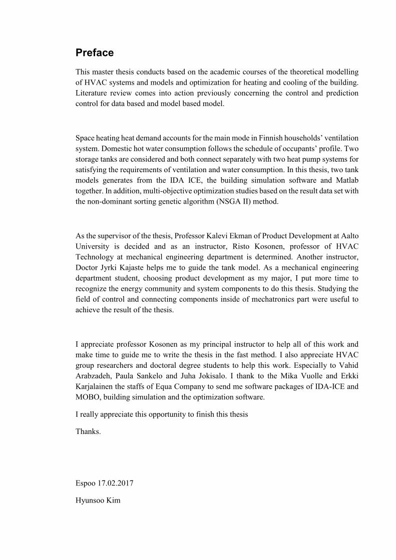
Preface
This master thesis conducts based on the academic courses of the theoretical modelling
of HVAC systems and models and optimization for heating and cooling of the building.
Literature review comes into action previously concerning the control and prediction
control for data based and model based model.
Space heating heat demand accounts for the main mode in Finnish households’ ventilation
system. Domestic hot water consumption follows the schedule of occupants’ profile. Two
storage tanks are considered and both connect separately with two heat pump systems for
satisfying the requirements of ventilation and water consumption. In this thesis, two tank
models generates from the IDA ICE, the building simulation software and Matlab
together. In addition, multi-objective optimization studies based on the result data set with
the non-dominant sorting genetic algorithm (NSGA II) method.
As the supervisor of the thesis, Professor Kalevi Ekman of Product Development at Aalto
University is decided and as an instructor, Risto Kosonen, professor of HVAC
Technology at mechanical engineering department is determined. Another instructor,
Doctor Jyrki Kajaste helps me to guide the tank model. As a mechanical engineering
department student, choosing product development as my major, I put more time to
recognize the energy community and system components to do this thesis. Studying the
field of control and connecting components inside of mechatronics part were useful to
achieve the result of the thesis.
I appreciate professor Kosonen as my principal instructor to help all of this work and
make time to guide me to write the thesis in the fast method. I also appreciate HVAC
group researchers and doctoral degree students to help this work. Especially to Vahid
Arabzadeh, Paula Sankelo and Juha Jokisalo. I thank to the Mika Vuolle and Erkki
Karjalainen the staffs of Equa Company to send me software packages of IDA-ICE and
MOBO, building simulation and the optimization software.
I really appreciate this opportunity to finish this thesis
Thanks.
Espoo 17.02.2017
Hyunsoo Kim
Table of Contents
Tiivistelmä
Abstract
Preface
Table of Contents ............................................................................................................... I
Nomenclature ................................................................................................................... II
Abbreviations .................................................................................................................. III
1. Introduction ................................................................................................................... 1
1.1. Background ............................................................................................................ 1
1.2. Research objective and outline............................................................................... 3
1.3. Structure of Thesis ................................................................................................. 4
2. Energy breakdown of single famly house ..................................................................... 6
2.1. Background ........................................................................................................ 6
2.1.1 Single Family house model in the Finnish Building Types ............................ 9
2.1.2 Description of case study for two tanks with solar collector model ............. 11
2.2. ESBO plant set up and simulation .................................................................... 17
3. Structure of HVAC energy system .............................................................................. 28
3.1 Modelling of the system components ................................................................... 28
3.1.1 Air Handling Unit ........................................................................................... 31
3.1.2 Ground Source Heat Pump.............................................................................. 35
3.1.3 High temperature storage tank........................................................................ 38
3.1.4 Low temperature storage tank ........................................................................ 40
3.1.5 Solar Collector ............................................................................................... 41
4. Control strategy method for energy system ................................................................ 44
4.1 Simulation Based Control system ......................................................................... 44
4.1.1 Low temperature storage tank control............................................................. 47
4.1.2 High temperature storage tank control ............................................................ 50
4.1.3 Solar collector and low temperature storage tank control ............................... 51
4.2 Artificial Neural Network (ANN) for the structure of the decision variables ...... 52
5. Cost optimal solution method in energy building ....................................................... 54
5.1 General explanation of Life Cycle Cost ................................................................ 54
5.2 Multi Objective optimiztion method ..................................................................... 56
5.2.1 Non Dominant Sorting Genetic Algorithm II (NSGA II) ............................... 57

6. Validation and Discussion ........................................................................................... 60
7. Result ........................................................................................................................... 61
7.1 Control strategy result ........................................................................................... 62
7.1.1 The result of low temperature tank control strategy ....................................... 64
7.1.2 The result of high temperature tank control strategy ...................................... 71
7.1.3 The result of solar collector control strategy................................................... 74
7.2 Artificial neural network result ............................................................................. 76
7.3 Multi Objective optimization result ...................................................................... 84
7.3.1 Cost of energy components ............................................................................. 84
7.3.2 Optimal selection of two tanks and solar collector ......................................... 85
8. Conclusions ................................................................................................................. 90
References ....................................................................................................................... 93
Appendixes ...................................................................................................................... 97
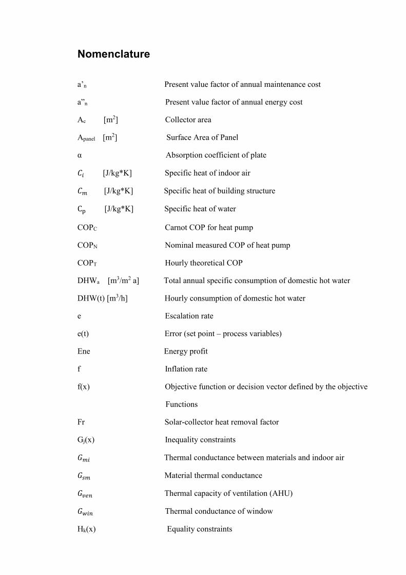
Nomenclature
a’n Present value factor of annual maintenance cost
a”n Present value factor of annual energy cost
Ac [m2] Collector area
Apanel [m2] Surface Area of Panel
α Absorption coefficient of plate
𝐶𝑖 [J/kg*K] Specific heat of indoor air
𝐶𝑚 [J/kg*K] Specific heat of building structure
Cp [J/kg*K] Specific heat of water
COPC Carnot COP for heat pump
COPN Nominal measured COP of heat pump
COPT Hourly theoretical COP
DHWa [m3/m2 a] Total annual specific consumption of domestic hot water
DHW(t) [m3/h] Hourly consumption of domestic hot water
e Escalation rate
e(t) Error (set point – process variables)
Ene Energy profit
f Inflation rate
f(x) Objective function or decision vector defined by the objective
Functions
Fr Solar-collector heat removal factor
Gj(x) Inequality constraints
𝐺𝑚𝑖 Thermal conductance between materials and indoor air
𝐺𝑠𝑚 Material thermal conductance
𝐺𝑣𝑒𝑛 Thermal capacity of ventilation (AHU)
𝐺𝑤𝑖𝑛 Thermal conductance of window
Hk(x) Equality constraints

h radiation [W/m2K] Heat Transfer coefficient
i Nominal interest rate
I [W/m2] Solar radiation density to solar collectors
Inv Investment cost for the sum of thermal solar-collector and
Tank price
Ki Integral gain, tuning parameter
Kp Proportional gain, tuning parameter
M Maintenance cost
ms Mass flow of air
n Holding period of investment
Qout Heating power of heat pump
��AHU Heat Power in the AHU
��Convection Heat Power from convection (φ𝑐)
��Domestic Heat Power inside of building
��equipment Internal heat gain from equipment
QHeating Internal heat gain from the coil of Air handling unit (AHU)
��Heatpump2 Heat power from the heat pump connected to the low
Temperature tank
��Low temperature tank Heat power from the low temperature tank
��machine Internal heat gain from machine
��materials + air Heat Power between materials and air
��materials Heat transfer in the material of the wall
��people Internal heat gain from people
��radiation Heat Power from radiation (φ𝑟)
��Solar collector Heat gain from the solar collector
��window Heat Power from window
��zone Heat Power in the building

r Real interest rate
re Escalated real interest rate
ρ Density of air
s Complex frequency
Ta Ambient temperature
Ta1 Temperature inside of AHU coil
Tc Collector average temperature
Tcon Condenser temperature
Teva Evaporator temperature
Tfi Flat-panel inlet fluid temperature inside of solar collector (K)
Tfo Flat-panel outlet fluid temperature inside of solar collector (K)
Ti Indoor temperature
Tm Temperature of the material node in the building structure
Tmix Temperature in the mixing box
To Temperature of outdoor air
Ts Temperature of ventilation (AHU) supply air node
Tr Room Temperature
Tpanel air Air temperature faced to the surface of the panel
Tsurface Surface temperature of the panel
Twin Supply air temperature of AHU
Twout Exhaust air temperature of AHU
U [W/m2K] Tank heat loss conductance
UL [W/m2] Solar collector heat loss coefficient
Welectric Electricity consumption of heat pump
φℎ𝑐 Space heating heat load
𝜏 Variable of integration
ηAHU Efficiency of AHU
Abbreviation
ANN Artificial Neural Network
BREEAM Building Research Establishment Environmental
Assessment Method
CAV Constant Air Volume
CHP Combined Heat and Power
CLO Clothing insulation
COP Coefficient of Performance
DH District Heating
DHW Domestic Hot Water
EA Evolutionary Algorithm
EC European Commission
EED Energy Efficiency Directive
EER Energy Efficiency Ratio
EPA Environmental Protection Agency
EPBD Energy Performance of Buildings Directive
EPC Energy Performance Certificate
ETS Emission-Trading System
g-value Total solar transmittance
GA Genetic Algorithm
GBC Green Building Council
GHG Green House Gas
GSHP Ground Source Heat Pump (Geothermal heat pump)
GUI Graphical User Interface
HEPAC Heating, Plumbing and Air Conditioning
HVAC Heating, Ventilation and Air Conditioning
IC Investment Cost
IDA ICE IDA Indoor Climate and Energy
IEA International Energy Agency
IFC Industry Foundation Classes
LEED Leadership in Energy and Environmental Design
LCC Life-Cycle Cost
MET Metabolic Equivalent
MOBO Multi-Objective Building Performance Optimization
NBCF National Building Code of Finland
NER300 New Entrant Reserve 300
NSGAII Non-Dominant Sorting Genetic Algorithm II
nZEB Nearly Zero Energy Building
PI Proportional integral
PMV Predicted Mean Vote
PPD Predicted Percentage of Dissatisfied
REHVA Federation of European Heating, Ventilation and Air
Conditioning Associations
SBO Simulation-Based Optimization
SPF Seasonal Performance Factor
SEER Seasonal Energy Efficiency Ratio
UNDP United Nations Development Program
UNEP United Nations Environment Program
VAV Variable Air Vol

1. Introduction
1.1 Background
European commission occupies the executive body of European Union (EU),
implementing decisions upholding the EU treats. In 2015, European commission leads
the project of the Energy Union to manage the stable supply of energy in European
market. The Energy Union is the modification of previous proposals of energy policies.
Previous European energy policies are composed of short term and long-term energy
strategies. Short term explains targets and strategies for 2020, 2030 and the long term is
to meet the gas reduction target through economic analysis that measures how to cost
effectively achieve decarbonization by 2050.
Energy strategy 2020 and 2030 (2030 energy strategy) aims to reduce greenhouse gas by
40% and contribute to renewable energy for amounts of 27% by the year of 2020 and
2030. Strategy 2050 (Energy Roadmap 2050) is achieving the 80% to 95% reduction in
greenhouse gasses compared to 1990 levels by the year of 2050. Moreover, this Energy
Union is implementing previous energy policies and meeting the decarbonization needs
of integrated European energy market for energy security, solidarity and trust. In
European energy market, energy efficiency and securing reliable energy in affordable
prices is the main challenge. To get the energy policies reliable, European Union keeps
three main goals; security of supply, competitiveness and sustainability for energy supply.
Security of supply is how to cope with unstable energy crisis depending on the Russia or
other neighbor countries’ states because of political issues. To disable unstable political
and economic situations, not only focusing one country for energy trading, but
diversifying supplier countries is necessary for the whole EU member countries. EU
energy import dependency accounts for 54% for all fuels. (Energy Roadmap 2050) To
cope with this, applying usable renewable energy as district heating is also another
method to respond the security of supply. Energy competitiveness and sustainability is
solutions to get the securities and stabilities as installing gas and oil pipelines and getting
the safe investment source for energy requirements. Adopting higher technologies to get
the better energy efficiencies is another method to pursue the energy competitiveness and
sustainability. To achieve three main goals, practical methods can negotiate. Main
strategy is reducing greenhouse gas, increasing higher energy efficiency and getting more
energy from renewables.
Finland has good energy source with biomass in this case. By the United Nations
Environment Program (UNEP), bioenergy accounts for 20 % of primary energy
consumption in Finland and 10 % of electricity demand. (Sustainable Buildings and
Climate initiative) By the International Energy Agency (IEA), Finland occupies the
highest energy consumption per capita among other countries. As other highly
industrialized countries conduct, energy efficiencies inside of industry is also main target
to achieve. Smart grid or district heating system inside of local city and the whole country
can belong to this target.
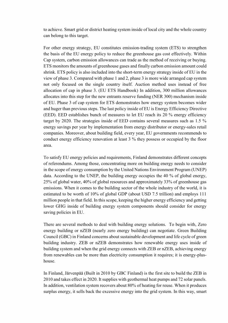
For other energy strategy, EU constitutes emission-trading system (ETS) to strengthen
the basis of the EU energy policy to reduce the greenhouse gas cost effectively. Within
Cap system, carbon emission allowances can trade as the method of receiving or buying.
ETS monitors the amounts of greenhouse gases and finally carbon emission amount could
shrink. ETS policy is also included into the short-term energy strategy inside of EU in the
view of phase 3. Compared with phase 1 and 2, phase 3 is more wide arranged cap system
not only focused on the single country itself. Auction method uses instead of free
allocation of cap in phase 3. (EU ETS Handbook) In addition, 300 million allowances
allocates into this step for the new entrants reserve funding (NER 300) mechanism inside
of EU. Phase 3 of cap system for ETS demonstrates how energy system becomes wider
and huger than previous steps. The last policy inside of EU is Energy Efficiency Directive
(EED). EED establishes bunch of measures to let EU reach its 20 % energy efficiency
target by 2020. The strategies inside of EED contains several measures such as 1.5 %
energy savings per year by implementation from energy distributor or energy-sales retail
companies. Moreover, about building field, every year, EU governments recommends to
conduct energy efficiency renovation at least 3 % they possess or occupied by the floor
area.
To satisfy EU energy policies and requirements, Finland demonstrates different concepts
of referendums. Among those, concentrating more on building energy needs to consider
in the scope of energy consumption by the United Nations Environment Program (UNEP)
data. According to the UNEP, the building energy occupies the 40 % of global energy,
25% of global water, 40% of global resources and approximately 33% of greenhouse gas
emissions. When it comes to the building sector of the whole industry of the world, it is
estimated to be worth of 10% of global GDP (about USD 7.5 trillion) and employs 111
million people in that field. In this scope, keeping the higher energy efficiency and getting
lower GHG inside of building energy system components should consider for energy
saving policies in EU.
There are several methods to deal with building energy solutions. To begin with, Zero
energy building or nZEB (nearly zero energy building) can negotiate. Green Building
Council (GBC) in Finland concerns about sustainable development and life cycle of green
building industry. ZEB or nZEB demonstrates how renewable energy uses inside of
building system and when the grid energy connects with ZEB or nZEB, achieving energy
from renewables can be more than electricity consumption it requires; it is energy-plus-
house.
In Finland, Järvenpää (Built in 2010 by GBC Finland) is the first site to build the ZEB in
2010 and takes effect in 2020. It supplies with geothermal heat pumps and 72 solar panels.
In addition, ventilation system recovers about 80% of heating for reuse. When it produces
surplus energy, it sells back the excessive energy into the grid system. In this way, smart

grid lets neighbor buildings connected for selling surplus energy and buying deficient
energy respectively.
In the scope of energy network system, two methods generally regards. For the electricity
network, smart grid system links among buildings with power station. Furthermore, for
the heat network system, it considers district heating, when natural gas piping usually
applies into the district heating network. In Finland, almost 80% of district heating
production based on Combined Heat and Power Generation (CHP) is equipped. In the
same time, one-third of electricity obtained from CHP generation operates and it is the
biggest figure inside of Europe by Finnish Energy (Finnish Energy, combined heat and
power generation). CHP plant usually builds up and applies in the Nordic countries for
energy efficiencies. While for other EU countries, CHP plant amounts for only around
10% of the whole electricity production, Finland occupies the most in energy producing
method. Because CHP employs leftover heat after electricity generation, into other heat
usage through hot water system. Thus, it is more energy efficient and useful than other
plant, which lets used-energy, go into the cooling tower or flue gas.
In this thesis, energy system inside of house considers to connect with district heating and
grid system when energy offers from CHP plant in Finland. However, in most cases,
energy system and components inside of building are zoomed in more than explaining
the grid system and district-heating network connected through the energy components.
For the energy components set up, higher energy efficient system components equipped
with present Finnish building demonstrates with two heat pumps and solar collector
before describing space heating and domestic hot water system. Sample building regards
as single-family house in simulation software and this house installs inside of Helsinki
Area in Finland. For the lower carbon society, energy policies and strategies in EU could
consider for building model. Less energy consumption inside building model can lead to
the energy saving in the whole industry.
1.2 Research objective and outline
The objective of this thesis is to study optimal design and control of thermal solar storage
system with two tanks model and get the optimal size of two thermal tanks and the area
of solar collector. This building model acknowledges connecting with the grid and
districting heating network; heat pump components connects to the grid and district
heating network communicates with the thermal solar collector on the roof of the house.
Purchasing the electricity from the grid does not calculate inside of the system, less
consumption of electricity from heat pump recommends for choosing the suitable size of
tanks and solar collector in the view of optimization. Keeping less electricity usage and
the higher efficiency of energy system is the main goal of this thesis.
Energy efficient building designs with two ground source heat pumps with two thermal
tanks and one solar collector. Building model generates from the simulation software IDA

ICE (version 4.7.1). Control and the optimization completes with Matlab using the Life
Cycle Cost (LCC) considering fluctuating economic parameter.
To get the optimal size of thermal tanks and solar collector, heat demand from the
radiating system, which directly connected to the AHU and generally used for space
heating heat demand and hot water consumption for the occupants is considered. Space
heating usually works from the Air Handling Unit and hydraulic system called radiator.
In Finland, heating the building during winter season is more important than cooling in
summer season. Compared with Energy Efficiency Ratio (EER) with air conditioning
performance system, reckoning Coefficient of performance (COP) on, especially heating
COP of heat pump demonstrates for calculating electricity consumption. Energy system
only considers sensible heat not regarding latent heat. Domestic hot water is consumption
of water usage depending on the occupants’ behavior. This building considered as single-
family house, high temperature tank connects for offering domestic hot water for the
whole building. Before offering hot water through high temperature tank, lower
temperature tank uses for preheating and space heating.
In this way, two tanks are connected each other and separately employed for space heating
and usage of domestic water consumption. Achieving thermal comfort, energy saving and
energy efficiencies with the lowest price is important goal to conduct. After making the
building model, heat demands gathered from the IDA ICE software and connection of
two-tank model completes from the Matlab software for the control modelling. Two tank
models generated from the schematic beforehand demonstrates to explain the different
heat demand and functions between low temperature tank and high temperature tank. For
control is dependent on the temperature for each tank model and building model,
schematic of single family house with energy system components are required.
Optimization shows how two objective function works for satisfying the less electricity
consumption in geothermal heat pumps and high efficiency of the building model using
solar collector in the system.
1.3 Structure of thesis
High-energy efficient type of building relies on the heating or cooling performance inside
of system components. Improving the heating or cooling performance along with
substantial energy savings could conduct by activating energy efficiency measures.
Electricity consumption of the heating, ventilation and air-conditioning(HVAC) system
occupies the most part, 40% of the whole building energy usage in the residential and
commercial building by the US. Energy Information Administration data. Thesis employs
three types of building to get the effect of insulation and selects suitable energy
components for higher building efficiencies and cost of components.
Literature review accomplishes beforehand starting thesis work. In most cases literature
review was checked that how predictive control with model based and data based control
can be done in other articles. Those categorize with different types of predictive control
method. This literature review was helpful in the view of control chapter before
conducting optimization.
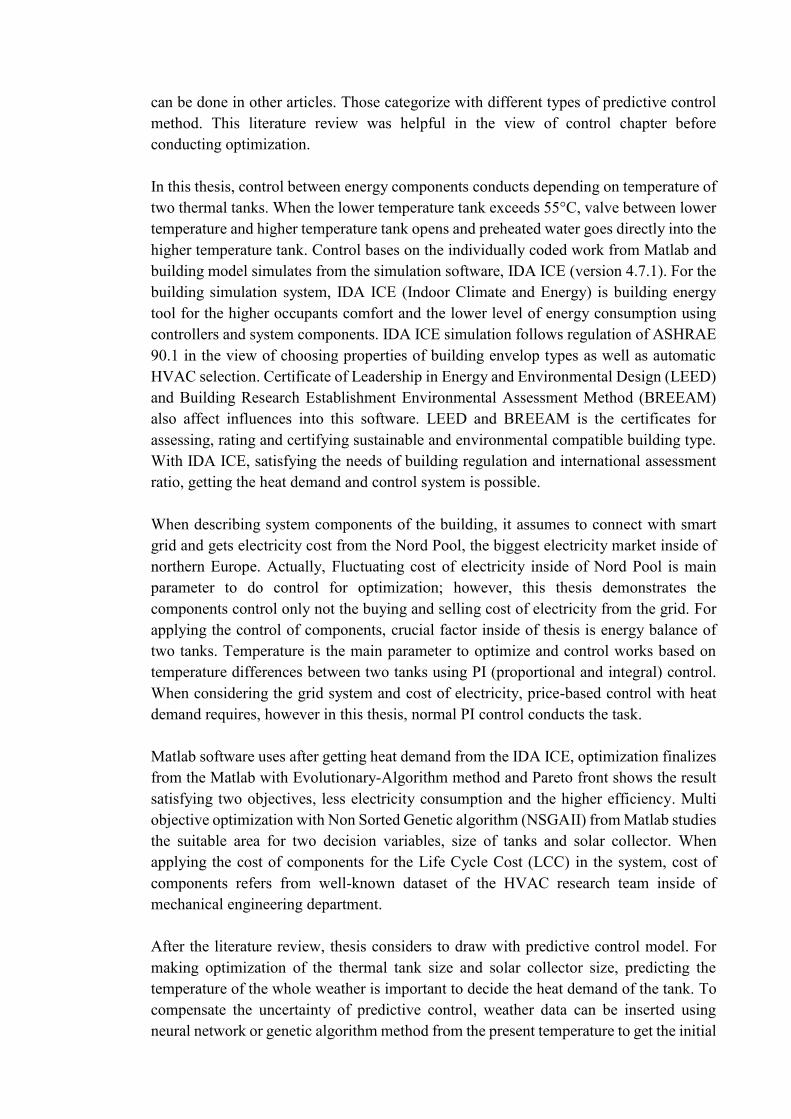
In this thesis, control between energy components conducts depending on temperature of
two thermal tanks. When the lower temperature tank exceeds 55°C, valve between lower
temperature and higher temperature tank opens and preheated water goes directly into the
higher temperature tank. Control bases on the individually coded work from Matlab and
building model simulates from the simulation software, IDA ICE (version 4.7.1). For the
building simulation system, IDA ICE (Indoor Climate and Energy) is building energy
tool for the higher occupants comfort and the lower level of energy consumption using
controllers and system components. IDA ICE simulation follows regulation of ASHRAE
90.1 in the view of choosing properties of building envelop types as well as automatic
HVAC selection. Certificate of Leadership in Energy and Environmental Design (LEED)
and Building Research Establishment Environmental Assessment Method (BREEAM)
also affect influences into this software. LEED and BREEAM is the certificates for
assessing, rating and certifying sustainable and environmental compatible building type.
With IDA ICE, satisfying the needs of building regulation and international assessment
ratio, getting the heat demand and control system is possible.
When describing system components of the building, it assumes to connect with smart
grid and gets electricity cost from the Nord Pool, the biggest electricity market inside of
northern Europe. Actually, Fluctuating cost of electricity inside of Nord Pool is main
parameter to do control for optimization; however, this thesis demonstrates the
components control only not the buying and selling cost of electricity from the grid. For
applying the control of components, crucial factor inside of thesis is energy balance of
two tanks. Temperature is the main parameter to optimize and control works based on
temperature differences between two tanks using PI (proportional and integral) control.
When considering the grid system and cost of electricity, price-based control with heat
demand requires, however in this thesis, normal PI control conducts the task.
Matlab software uses after getting heat demand from the IDA ICE, optimization finalizes
from the Matlab with Evolutionary-Algorithm method and Pareto front shows the result
satisfying two objectives, less electricity consumption and the higher efficiency. Multi
objective optimization with Non Sorted Genetic algorithm (NSGAII) from Matlab studies
the suitable area for two decision variables, size of tanks and solar collector. When
applying the cost of components for the Life Cycle Cost (LCC) in the system, cost of
components refers from well-known dataset of the HVAC research team inside of
mechanical engineering department.
After the literature review, thesis considers to draw with predictive control model. For
making optimization of the thermal tank size and solar collector size, predicting the
temperature of the whole weather is important to decide the heat demand of the tank. To
compensate the uncertainty of predictive control, weather data can be inserted using
neural network or genetic algorithm method from the present temperature to get the initial
input data for the predictive model. However, in this thesis, only temperature is main
parameter and it considers energy balance briefly for the more accurate data output and
validating the result. When optimizing the multi objective model, accurate weather input
data is important than conceptual weather input, thus present weather data is employed
as the form of vector to lead the correct output. For the present weather data, Helsinki-
Vantaa weather is used and IDA software operates for the one-year working input data.
Building model is single-family house with first and second floors. Occupancy behaviors
and lighting data refers from the minimum requirements of Finnish building with code
C3, thermal insulation code for the Finnish building. Three different type of building
operates for getting the heat demand result from the simulation software. Lightweight,
medium weight and massive passive weight building are employed and thermal
insulations used inside of building envelop are different depending on types.
For the more accurate data result, validation conducts with IDA ICE and MOBO (Multi-
Objective Building Performance Optimization) software. Validation result compares with
generated one tank model with IDA ICE and Matlab together. Validation result
demonstrates similar trend of output and it verifies this two tanks model.
2. Energy breakdown of single family house
2.1 Background
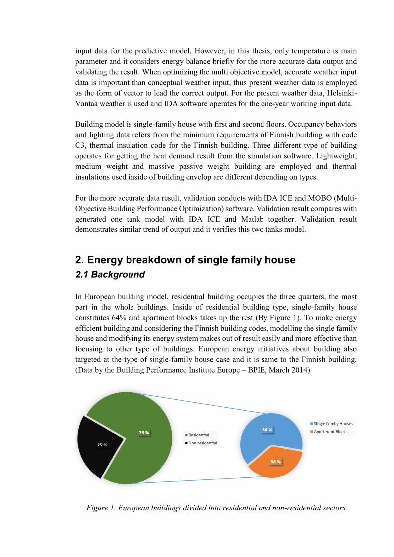
In European building model, residential building occupies the three quarters, the most
part in the whole buildings. Inside of residential building type, single-family house
constitutes 64% and apartment blocks takes up the rest (By Figure 1). To make energy
efficient building and considering the Finnish building codes, modelling the single family
house and modifying its energy system makes out of result easily and more effective than
focusing to other type of buildings. European energy initiatives about building also
targeted at the type of single-family house case and it is same to the Finnish building.
(Data by the Building Performance Institute Europe – BPIE, March 2014)
Figure 1. European buildings divided into residential and non-residential sectors
Finnish houses are more restricted about the density of population compared with other
European houses even though its high quality of living conditions. Amounts of dwelling
(2.9million) exceeds the number of households (2.6million) and the common size of
average household is 2.05 person. Another pattern is one or two consisting households
manage 75% of Finnish dwellings. (By the Hannonen et al.) For this pattern, optimizing
the building components of single-family house is more required than any other building
type. In this thesis, following the trend of building types in European countries and
Finland, it employs single-family house as the model of the house. Especially it choses
Finnish current building with two-story house for modelling and optimization.
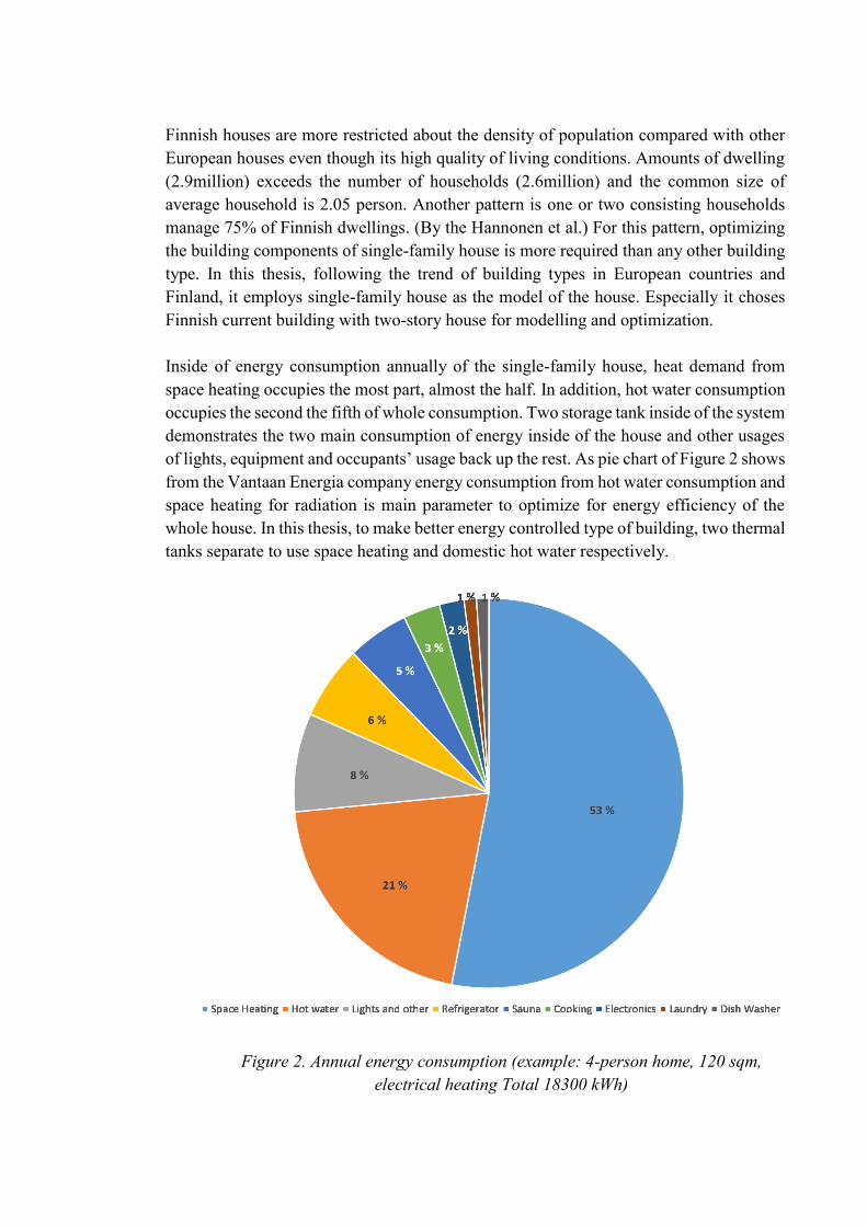
Inside of energy consumption annually of the single-family house, heat demand from
space heating occupies the most part, almost the half. In addition, hot water consumption
occupies the second the fifth of whole consumption. Two storage tank inside of the system
demonstrates the two main consumption of energy inside of the house and other usages
of lights, equipment and occupants’ usage back up the rest. As pie chart of Figure 2 shows
from the Vantaan Energia company energy consumption from hot water consumption and
space heating for radiation is main parameter to optimize for energy efficiency of the
whole house. In this thesis, to make better energy controlled type of building, two thermal
tanks separate to use space heating and domestic hot water respectively.
Figure 2. Annual energy consumption (example: 4-person home, 120 sqm,
electrical heating Total 18300 kWh)
By the pie chart of this result, domestic hot water and space heating occupies in the most
case for annual energy consumption of the house. Space heating is heating method in the
limited room with radiator or employing floor-heating method. Domestic hot water is
water consumption method from the cold water supply to the hot water offering for the
kitchen or bathroom. It can also use as radiating system or boiler, pipeline between the
hot and cold waters are different.
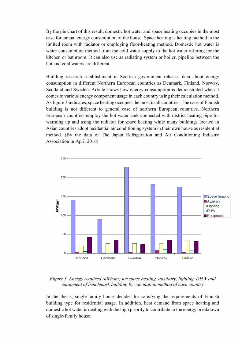
Building research establishment in Scottish government releases data about energy
consumption in different Northern European countries as Denmark, Finland, Norway,
Scotland and Sweden. Article shows how energy consumption is demonstrated when it
comes to various energy component usage in each country using their calculation method.
As figure 3 indicates, space heating occupies the most in all countries. The case of Finnish
building is not different to general case of northern European countries. Northern
European countries employ the hot water tank connected with district heating pipe for
warming up and using the radiator for space heating while many buildings located in
Asian countries adopt residential air conditioning system in their own house as residential
method. (By the data of The Japan Refrigeration and Air Conditioning Industry
Association in April 2016)
Figure 3. Energy required (kWh/m²) for space heating, auxiliary, lighting, DHW and
equipment of benchmark building by calculation method of each country
In the thesis, single-family house decides for satisfying the requirements of Finnish
building type for residential usage. In addition, heat demand from space heating and
domestic hot water is dealing with the high priority to contribute to the energy breakdown
of single-family house.
Influence of energy efficiency from the background of Kyoto protocol, Finnish energy
and climate strategy aims to reduce the greenhouse gas emission. Technical regulations
and instructions from the Ministry of the Environment degree arranged seven different
sections from Finnish building code. In the view of energy efficiency of building, D3
regulation decides clause from 2012 for building regulations and guidelines while D5 is
the calculation of energy consumption and heat loss of the building and the last C4 code
generates for the thermal insulation instructions. As this regulation defines, D section is
applied by the data from ‘HEPAC (Heating, Plumbing and Air Conditioning)’and energy
management. E indicator (so called E-value) is key driver to permit the energy
consumption of the building and D5 stipulates with grid system. D3 is general guideline
for the Finnish building and decides the ventilation efficiency and supply air rate to the
building when different type of building applies. Temperature to keep constant for
ventilation decides by the building guideline in the D section. Efficiency of building
envelope is different by the insulation material to use, C4 states in the
Ympäristöministeriö, 2012, the Finnish building code.
2.1.1 Single Family house model in the Finnish Building Types
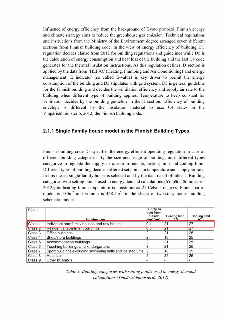
Finnish building code D3 specifies the energy efficient operating regulation in case of
different building categories. By the size and usage of building, nine different types
categorize to regulate the supply air rate from outside, heating limit and cooling limit.
Different types of building decides different set points in temperature and supply air rate.
In this thesis, single-family house is selected and by the data result of table 1. Building
categories with setting points used in energy demand calculations (Ympäristöministeriö,
2012); its heating limit temperature is constraint as 21-Celsius degrees. Floor area of
model is 180m2 and volume is 468.1m3, in the shape of two-story house building
schematic model.
Table 1. Building categories with setting points used in energy demand
calculations (Ympäristöministeriö, 2012)
Class
Building type
Supply air rate from outside
(dm3/sm2) Heating limit
(C°) Cooling limit
(C°)
Class 1 Individual one-family houses and row houses 0.4 21 27
Class 2 Residential apartment buildings 0.5 21 27
Class 3 Office buildings 2 21 25
Class 4 Shop/store buildings 2 18 25
Class 5 Accommodation buildings 2 21 25
Class 6 Teaching buildings and kindergartens 3 21 25
Class 7 Sport buildings excluding swimming halls and ice stadiums 2 18 25
Class 8 Hospitals 4 22 25
Class 9 Other buildings - - -

When applying building model for getting the heat demand, indoor temperature considers
keeping as 21 Celsius degrees. Building in Finland with ground source heat pumps need
heating radiating system more than cooling system, thus building temperature considers
keeping as 21 degree and heating energy demand estimates for generating energy demand
of the building.
For the building envelope, this model of the house more focuses on the Finnish weather.
Finnish building is usually well isolated with insulations. Long term harsh winter season
affects enormous impact on Finnish building wall thickness and material in the building
type of Finland. (Subba et all 2015). To cope with harsh Finnish winter case, different
type of building envelope decides by the material and wall thickness following the Finnish
building code C4. Light weight, middle weight and massive passive weight of buildings
are decided and most of them have different insulations inside (Table 2) from the
comparison of 1960 Finnish building type with standard 2010 type in Alimohammadi et
al. 2014.
In the type of lightweight, materials are wood frame construction. Medium weight
building type is similar to the lightweight except of roof construction; concrete materials
employs into this structure. In addition, the massive weight building type, most of them
are concrete and equipped well for the long winter season in Finland. In this thesis, light
weight, medium and massive thermal mass buildings are used from the SAGA (Smart
Control Architecture for Smart grids 2012-2016) project, 2010 standard type for the
modelling and optimization in the type of single family house.
Table 2. Properties of different type of buildings in Standard 2010
For simulation from the SAGA project Aalto University (Alimohammadi et al. 2014)
Type of building
structures
Elements of
construction
Material composition (thickness of the layer)
/external structures from inside to outside
Overall
thickness(mm)
Light
External wall Gypsum (13 mm), wooden frame + mineral wool (540 mm), wind shield board (9 mm) 562
Internal wall Gypsum (13 mm), wooden frame (40 mm), gypsum (13 mm) 66
Roof Gypsum (13 mm), wooden frame + mineral wool (150 mm), mineral wool (375 mm), water proof sheet (10 mm) 548
Base floor Wood (14 mm), wooden frame + mineral wool (436 mm), wind shield board (9 mm) 459
Intermediate
floor Wood (15 mm), particle board (22 mm), wooden frame (150 mm), gypsum(13 mm) 200
Medium
External wall Gypsum (13 mm), wooden frame + mineral wool (540 mm), wind shield board (9 mm) 562
Internal wall Gypsum (13 mm), wooden frame (40 mm), gypsum (13 mm) 66
Roof Gypsum (13 mm), wooden frame + mineral wool (150 mm), mineral wool (375 mm), water proof sheet (10 mm) 548
Base floor Wood (14 mm), light weight concrete (15 mm), concrete (100 mm), EPS thermal insulation (480 mm) 459
Intermediate floor
Wood (15 mm), particle board (22 mm), wooden frame (150 mm), gypsum(13 mm) 200
Massive
External wall Light weight concrete block (130 mm), polyurethane (340 mm), light weight concrete block (90 mm) 560
Internal wall Light weight concrete block (100 mm) 100
Roof Filler (5 mm), concrete (100 mm), mineral wool (490 mm), water proof sheet (10 mm) 605
Base floor Wood (14 mm), light weight concrete (15 mm), concrete (100 mm), EPS thermal insulation (480 mm) 609
Intermediate
floor Wood (15 mm), light weight concrete (15 mm), concrete (100 mm), filler (5 mm) 135

In the single-family house modelling, two thermal tanks study for domestic hot water and
space heating. It employs low temperature tank for radiating the building envelope inside
the house and high temperature tank for tenants’ hot water consumption. Low temperature
tank requires more energy demand than domestic hot water tank for preheating the tank
and warming up the building envelope. To compensate energy needs for low temperature
tank, solar thermal installed on the roof of the house connects to the low temperature tank
operating the system. The sum of energy need from the building envelope and inner room
is same as the heat demand supplied from the Air Handling Unit on the ceiling of the
indoor building for radiating the whole system.
2.1.2 Description of case study for two tanks with solar collector model
Energy system inside of building model in the thesis is composed of two geothermal heat
pumps with thermal tanks and solar collector. From the modelling of the system, it
employs low temperature thermal tank for radiating the building inside and high
temperature thermal tank for hot water consumption. To make energy system more
efficient, appropriate heating, ventilation and air conditioning (HVAC) is the key factor
to keep the comfortable, healthy living and working environment inside of house.
Electricity consumption inside of the HVAC system occupies the 40% of the whole
building electricity consumption by the U.S.Green building Council (USGBC).
Improving the cooling and heating performance of the building with energy saving can
be achieved by implementing energy efficiency methods. Most suitable method is
focusing on the high-energy efficient HVAC system and choosing the suitable size of
components for the cost reduction and energy efficiency. In this thesis, it chooses
optimized size of tanks and solar collector to make current building as the better-adjusted
energy system.
In the building simulation software IDA ICE, it only generates one tank model with solar
collector. For higher energy-efficient building, two-tank model operating separately in
the use of domestic hot water and space heating is required. Schematic of building model
demonstrates how two tanks operate individually for the usage of domestic hot water
consumption and radiating. To control two tanks, temperature is main parameter and heat
balance should calculate before conducting the control and optimization. Self-coded
Matlab software shall finalize the control and optimization.
In the view of the satisfaction for the heat demand of different types of building, air
handling unit system connected to the low temperature tank and building together
supplies the whole energy into the building from the tank model. Inside of building model,
temperature difference and heat transfer discusses before getting heat demand. Building
model assumes to connect with air handling unit directly, outdoor air temperature contacts
to the wall of the building and air-handling unit directly. It shows below schematics as

figure 4. Figure 4 demonstrates how indoor air temperature and temperature of structure
decides by outdoor temperature and heat capacity factors.
To make room keeping temperature as 21˚C, heat supply from air handling unit is
regarded as same as gained heat from the whole building in the way of energy balance.
Inside of the building, gained thermal loads divide as two parts. One is convection thermal
loads and the other is radiation thermal loads in the view of space heating. Whole energy
transfer inside of room derives from the low temperature tank and it transfers energy into
the Air Handling unit and building.
ToGwi
Gsm
Ti
GvenTs
Φc (convection)
Φr (radiatio
n)
CmAmTm
Gmi
Gmi
Tm
To
Φhc
Gwi
To
Gmi
Tm
Ti
Gsm
Cm
Ci
φc
φrφhc
Figure 4. Equivalent electro circuit representing the heat transfer in the
specified building boundary system
The whole heat demand of the building is same as the heat transfer from the low
temperature tank to the Air Handling unit. When energy transfer occurs from the low
temperature tank to the Air Handling unit, energy passes through material of the wall,
shell of window and air between wall and indoor air. How heat transfer occurs through
the wall and window shows in the schematic of figure 4. Left picture demonstrates
direction of heat transfer from the outside to the inside of the building with the method of
conduction, convection and radiation. Right picture shows detail heat transfer by electro
circuit in the restricted building boundary of single-family house in the way of
conduction.

Heat gain from the zone (equation 1) is summation heat between wall insulation and air,
wall materials and air conduction inside of the room.
�� zone = �� AHU = �� materials + air + �� materials + �� domestic + �� window + �� convection + �� radiation
(1)
where
��zone Heat Power in the building
��AHU Heat Power in the AHU
��materials + air Heat Power between materials and air
��materials Heat transfer in the material of the wall
��domestic Heat Power inside of building
��window Heat Power from window
��convection Heat Power from convection
��radiation Heat Power from radiation
Heat gain from convection (equation 2) is the total sum of the gained heat from equipment,
occupants’ behavior and machine.
��convection = ��equipment + ��people + ��machine (2)
where
��convection Convection heat load (φ𝑐)
��equipment Internal heat gain from equipment
��people Internal heat gain from people
��machine Internal heat gain from machine
Radiating heat gain (equation 3) is energy demand from the space heating and this one
connects with the low temperature tank of the above energy system mentioned before.
Radiation energy describes to get from equation 3. Area of radiator and temperature
between panel and surface decides for the heat demand of radiation by the Tähti et al.
��radiation = Σ ℎradiation *Apanel *(Tpanel air - Tsurface) (3)
where
��radiation Heat power from radiation (φ𝑟)
ℎradiation Heat Transfer coefficient (Wm-2K-1)
Apanel Surface Area of panel
Tpanel air Air temperature faced to the surface of the panel
Tsurface Surface temperature of the panel
Temperature of inside of the building calculates considering the material temperature
between the building walls. Equation (4) shows how material temperature is decided by
the radiation heat load and the heat gain from the outside temperature, material
temperature and indoor temperature.
𝐶𝑚𝑑𝑇𝑚
𝑑𝑖 = 𝐺𝑠𝑚(𝑇𝑜 - 𝑇𝑚) + 𝐺𝑚𝑖(𝑇𝑖 - 𝑇𝑚) + φ𝑟 (4)
where
𝐶𝑚 Heat capacity of building structure
𝐺𝑠𝑚 Material thermal conductance
𝐺𝑚𝑖 Thermal conductance between materials and indoor air
𝑇𝑜 Temperature of outdoor node
𝑇𝑚 Temperature of material node
φ𝑟 Radiation heat load
Equation (5) demonstrates the amounts of space heating heat load is required in the view
of balance equation for the indoor heat gain.
𝐶𝑖𝑑𝑇𝑖
𝑑𝑡 = 𝐺𝑣𝑒𝑛(𝑇𝑠 - 𝑇𝑖) + 𝐺𝑤𝑖(𝑇𝑜 - 𝑇𝑖) + 𝐺𝑚𝑖(𝑇𝑚 - 𝑇𝑖) + φ𝑐 + 𝝋𝒉𝒄 (5)
where
𝐶𝑖 Heat capacity of indoor air
𝐺𝑣𝑒𝑛 Thermal capacity of ventilation (AHU)
𝐺𝑤𝑖𝑛 Thermal conductance of window
𝐺𝑚𝑖 Thermal conductance between materials and indoor air
𝑇𝑠 Temperature of ventilation (AHU) supply air node
𝑇𝑚 Temperature of material node
𝑇𝑖 Temperature of indoor air
φ𝑐 Convection heat load
φℎ𝑐 Space heating heat load
Indoor temperature of the house should keep as 21˚C. It decides indoor temperature for
24 hours without space heating heat load, by the initial temperature in the way of Euler
implicit method and indoor temperature fluctuates by the conductance of window, AHU,
conductance between material and air and the convection heat load. To make indoor
temperature constant, space heating with ventilation system is required. Formulae (6)
demonstrates how indoor temperature keeps constant while every time step tries with
Euler Implicit method. Time step is 1 hour and new approximation (unknown variable)
is dependent on the previous indoor temperature node. By iterating initial temperature
value, it generates 8760 samples in the end. It is one-year data when IDA simulation
adopts.
𝑇𝑖𝑛 =
𝐶𝑖
𝛥𝑡𝑇𝑖
𝑛−1+ 𝐺𝑣𝑒𝑛∗𝑇𝑠 + 𝐺𝑤𝑖∗𝑇𝑜 + 𝐺𝑚𝑖∗𝑇𝑚+ φ𝑐+ 𝝋𝒉𝒄
𝐶𝑖
𝛥𝑡+𝐺𝑣𝑒𝑛+𝐺𝑤𝑖+𝐺𝑚𝑖
(6)
where
n number of iteration
Temperature of material node shows with thermal conductance of material node,
conductance between material and air, radiation heat load and previous temperature of
material node with Euler implicit method. (Equation 7)
𝑇𝑚𝑛 =
𝐶𝑚
𝛥𝑡𝑇𝑚
𝑛−1+ 𝐺𝑠𝑚∗𝑇𝑜 + 𝐺𝑚𝑖∗𝑇𝑖−1 + φ𝑟
𝐶𝑚
𝛥𝑡+𝐺𝑠𝑚+𝐺𝑚𝑖
(7)
Euler method presents, when equation (6) and (7) combines, space heating heat load
decides by this sum up.
φhc = (Gven + Gwi + Gmi)*Ti – Gwi*To – Gven*Ts – Gmi*Tm - φc (8)

Space heating is dependent on the indoor temperature, outdoor temperature and
convection heat load. As discussed previous, convection heat load is the gross sum of
gained inner heat from equipment, machine and tenants’ behaviors of the building model.
To calculate heat load from the simulation software, it is necessary to draw house model
and make a separate zone by different rooms and spaces inside. Figure 5 demonstrates
how different materials applies into the walls by visualization. Floor area of 180m2,
volume of 468.1 m3 model adopts to this single-family house.
Figure 5. Visualization of two story building in the form of single-family when passive
massive material adopts.
Lightweight, medium weigh and passive massive weight of materials applies into the wall
of the building for insulation. In this figure, passive massive materials are studied thus
concrete are used for thick wall structure. To make inner temperature of building keep
constant, minimum usage of electricity in heat pump for space heating is required for the
efficient method of energy system. Energy efficiency system with two heat pumps and
two thermal tanks with solar collector can design inside of simulation software. Single-
family house CAD file is imported as IFC (Industrial Foundation Classes) format into the
IDA software for exact zoning the building and getting the heat demand data from each
space. Inside of the whole building, spaces merge and zone as three different places for
accurate calculation.
After operating building model, heat demand from the space-heating tank and domestic
hot water tank works separately and connected through the Matlab code. Space heating
heat demand is dependent on the equation (8) by the temperature of time step from the
Euler Method. Domestic hot water is following the profile schedule of the occupants
inside. When applying this work, energy balance uses for exact calculation. Inside of IDA
ICE software, usually one thermal tank with one heat pump generates with solar collector
system. For operating two heat pumps with two thermal tanks, operating three samples
simultaneously as parallel method and combining them is required to get the result data.
When initial data is decided, using default platform called Early Stage Building
Optimization (ESBO) Plant; energy system is set and operated with components.
2.2 ESBO plant set up and simulation
IDA ICE is building simulation software for indoor climate and energy. It is specified
version of General IDA software and contains more indoor individual zone control for
the complete building envelope. When IDA ICE simulation software employs, it receives
initial input data from users. Users can choose or make their own weather vector by
outdoor temperature, humidity, wind speed and radiation and temperature from solar
energy. From version 4.5, IDA ICE shows new wizard interface called ESBO (early stage
building optimization) and updated room wizard. Installed wizard, ESBO plant mainly
uses for generating the building model with energy components.
ESBO plant is building-optimization simulation program with different geometry of
building drawing. Various insulation and envelopes adopts to the building connecting
solar thermal and tank system. External and internal walls, roof and floor materials are
object to passive massive, medium and lightweight building envelope. Selecting materials
for insulation of building, connecting central system with ESBO plant is required. ESBO
plant materializes the drawing and type of building importing CAD objects and images.
Building information models (BIM), CAD and vector graphic files can execute for
operating IDA ICE building model. BIM contains properties of the house and 3D
geometries as zoning rooms, window and building body. It automatically generates the
data objects from mapping the IFC dialog. Two story building in single-family house type
creates from the SAGA project by the Alimohammadi et al. 2016. As figure 6
demonstrates below. After adopting the template building drawing from IFC mapping,
merging the zone is necessary to install two-story single-family house for 3D model.

Figure 6. IFC imported file of single-family house of 2nd story building type
After that by the ESBO plant, components choose in the plant set up and used inside of
the building energy system. However, this is one tank model with solar collector thus,
installing two different type of building, one for the domestic hot water and the other for
the radiating is demanding. Getting the heat demand and combining two tanks with one
tank model comes into action with Matlab software. Row vector from the utilized energy
puts to use to finalize the tank model and this conducts by the individually defined codes
in the Matlab software.
Generally, solar thermal and photovoltaic connects to the single-family house with hot
storage tank and heat pump component. In this thesis, ground source heat pump applies
to combine with the tank. Coefficient of Performance (COP) of the heat pump is four, but
it can be different in condensing temperature and evaporating temperature. (By Yrjölä et
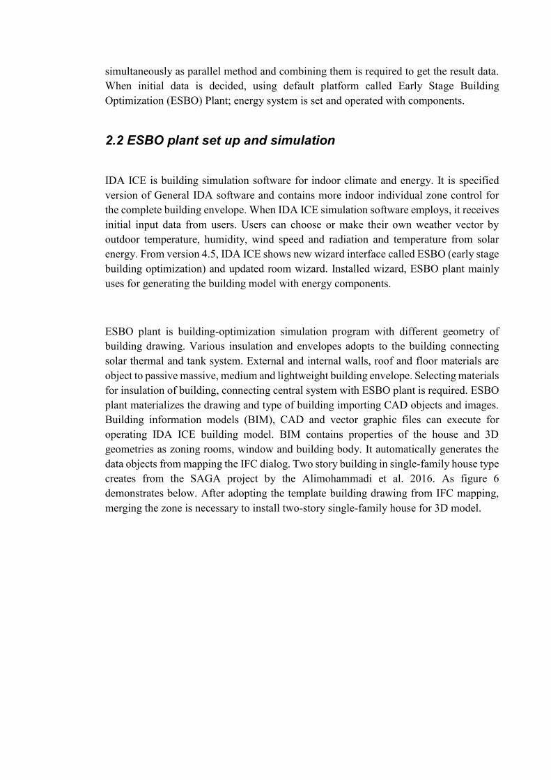
al.) Indoor climate condition regulates as basic setting for making the room temperature
and air quality constant (Figure 7). Keeping indoor temperature constant is main initial
input for the heat balance and in the view of getting the energy transfer from the tank and
solar collector to the room of the single-family house.
Figure 7. Indoor room condition with temperature and CO2 for thermal comfort
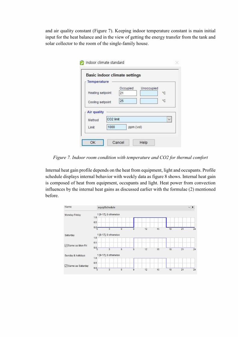
Internal heat gain profile depends on the heat from equipment, light and occupants. Profile
schedule displays internal behavior with weekly data as figure 8 shows. Internal heat gain
is composed of heat from equipment, occupants and light. Heat power from convection
influences by the internal heat gains as discussed earlier with the formulae (2) mentioned
before.

Figure 8. Schedule of Equipment, occupants and light from the internal heat gain
profile
Selecting energy components and simulating with ESBO plant is required for getting the
heat demand of the system. In ESBO plant, one tank model generally introduces
connecting with space heating and domestic hot water consumption usage as Figure 9
demonstrates.

Figure 9. ESBO plant for the domestic hot water and space heating connection
with one tank and solar collector
In this thesis, smart grid system considers connecting for buying and selling the electricity
usage of the building, however photovoltaic is not applied. Instead, solar thermal is
considered to be connected to the district heating and adopted for the compensating the
heat pump operation when solar radiation and energy works. Solar thermal area changes
from 1m2 to 10m2 for the optimization, while its installation angel keeps as 45 ° fixed and
its orientation defines as 0 ° as Figure 10 demonstrates.

Figure 10. Schematic of solar thermal in ESBO plant
Hot storage assumes to be the tank component in the shape of cylinder for linking pipe of
the water consumption usage and radiation. Hot storage has eight layers and stratified
tank system applies for the exact temperature calculation. Layer of the tank varies from
one to the 50, in this thesis, eight layers assumes and temperature variation happens in
different layers. Insulation U value for the tank is 0.3W/m2 °C and shape factor
(height/diameter) of the cylindrical tank is five. This is initial input value for the energy
computation.
In the heat pump components, brine to water heat pump applies as ground source heat
pump and its type is reciprocating type with COP of the four like Figure 11 shows.
Minimum evaporator temperature and condensing temperature is set as -50°C and 70°C
respectively while brine evaporator temperature and hot water condensing temperature
regulates as each 8°C individually. Water type brine uses in the heat pump and the
auxiliary heater is equipped with the tank for running the boiler with pump system.
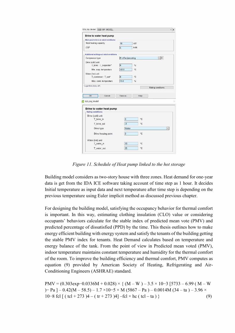
Figure 11. Schedule of Heat pump linked to the hot storage
Building model considers as two-story house with three zones. Heat demand for one-year
data is get from the IDA ICE software taking account of time step as 1 hour. It decides
Initial temperature as input data and next temperature after time step is depending on the
previous temperature using Euler implicit method as discussed previous chapter.
For designing the building model, satisfying the occupancy behavior for thermal comfort
is important. In this way, estimating clothing insulation (CLO) value or considering
occupants’ behaviors calculate for the stable index of predicted mean vote (PMV) and
predicted percentage of dissatisfied (PPD) by the time. This thesis outlines how to make
energy efficient building with energy system and satisfy the tenants of the building getting
the stable PMV index for tenants. Heat Demand calculates based on temperature and
energy balance of the tank. From the point of view in Predicted mean voted (PMV),
indoor temperature maintains constant temperature and humidity for the thermal comfort
of the room. To improve the building efficiency and thermal comfort, PMV computes as
equation (9) provided by American Society of Heating, Refrigerating and Air-
Conditioning Engineers (ASHRAE) standard.
PMV = (0.303exp−0.0336M + 0.028) × { (M – W ) – 3.5 × 10⁻³ [5733 – 6.99 ( M – W
)− Pa ] – 0.42(M – 58.5) – 1.7 ×10⁻⁵ × M (5867 – Pa ) – 0.0014M (34 – ta ) – 3.96 ×
10−8 fcl [ ( tcl + 273 )4 – ( tr + 273 )4] –fcl × hc ( tcl – ta ) } (9)
where
M Metabolism rate
W External Work
Pa Partial water vapor pressure
ta Air temperature
fcl Thermal resistance of clothing
tcl Surface temperature of clothing
hc Convective heat transfer coefficient
tr Radiant temperature
ta Air temperature
The recommended acceptable PMV range for thermal comfort from ASHRAE 55 is
between -0.5 and +0.5 for an interior space. From the view point of PMV, air temperature,
radiant temperature, relative humidity and air velocity stays inside of comfort bounds and
control system contributes to the scope of the comfort level.
In the IDA ICE, PI (Proportional Integral) controller adopts to respond temperature
control of the simulation. Control system works based on the temperature sensor and PI
controller system connected to the tanks and solar collector. Sensor and controller holds
up the temperature signal to be in accepted range for the thermal comfort of the building
envelope. PI controller is control loop feedback mechanism generally used in building
control and optimization. Error value calculates measuring the difference from the set
point of the temperature and processed variables, then calibrates it with proportional and
integral method. Formulae (10) demonstrates manipulated variables from the sum up of
proportional and integral terms. (11) is the transfer function in the Laplace domain of PI
control.
u(t) = Kpe(t) + Ki∫ 𝑒(𝑡
0𝜏) (10)
L(s) = Kp+Ki/s (11)
where
Kp Proportional gain, tuning parameter
Ki Integral gain, tuning parameter
e(t) Error (set point – process variables)
t time

𝜏 Variable of integration
s Complex frequency
Inside of IDA ICE, temperature set completes by the set point as figure 12 shows.
Minimum and maximum temperature is set and in the heating mode, Proportional control
works with radiator and in the cooling mode, PI controller runs in the actual device for
the steady state of temperature in the fluctuation situation.
Figure 12. Set point collections with PI control method inside of IDA ICE
In the hot tank storage, temperature for radiation and space heating is determined
approximately 45°C and temperature for domestic hot water consumption is set as 60°C.
When it comes to the IDA ICE hot storage tank, its temperature variation inside of
stratified tank has eight layers with different temperature range.

In this thesis, two thermal tank model with two ground source heat pumps are discussed
different from general IDA ICE tank system. Typical system for IDA ICE is one tank
model linked to one heat pump with solar collector or PV system. To satisfy the need of
two storage tanks, one tank manages the space heating inside of building envelope and
the other runs the domestic hot water consumption heat demand of the house. Thesis
determines how to connect two tanks with Matlab coded simulation and shall check the
result with multi-objective optimization method.
Lower temperature tank with solar collector operates in the beginning. Moreover, lower
temperature tank without solar collector operates in the next step. Both cases contain only
space heating case not considering hot water consumption. In this case, only building
radiation finalizes with space heating method however, hot water consumption is zero. In
addition, the last, higher temperature tank is operating with domestic hot water
consumption not thinking about radiating the building work. After these three samples
are operating with parallel method, optimization also to be considered depending on area
of solar collector and size of tanks. Size of hot storage tank is changing from 0.5 m3 to 2
m3 with step of 0.5 m3 during the size of solar collector goes from 1 m2 to 10 m2 with step
as 1m2. Lower temperature tank without solar collector and higher temperature tank only
for the domestic hot water model generates four samples respectively and lower
temperature tank with solar collector model has 40 samples. Thus, after conducting
parallel method 48 samples generate the result. When building type is three different type;
lightweight, medium weight and massive weight, 144 samples are finally get from the
simulating the building model from the IDA ICE software.
HEAT Pump 1
SolarCollector
BuildingLT
HT
LT Te
To
TsTi
Cold water(7˚C )
TwinTwout
HEAT Pump 2
21˚C
High Temperature tank
Low Temperature tank
Building control
Figure 13. Schematic of the whole energy system of components
In the two tanks, low temperature tank uses for space heating and high temperature tank
employs as hot water consumption. Two tanks employ different temperature individually;
IDA ICE operates low temperature and high temperature tank separately for this thesis.
When PI controller for the room fixes to make indoor temperature keeping as 21 ˚C, low
temperature tank supplies heat for Air Handling Unit to supply energy demand for the
building model. Figure 13 demonstrates how two-thermal storage tanks with heat pumps
are operating and connected. For this running, temperature of three main control system
is required; low temperature tank, high temperature tank with solar collector and building
inner temperature with Air Handling Unit. High temperature tank keeps temperature as
60°C and low temperature tank keeps as 45°C connected to the solar collector. In addition,
the temperature of building keeps temperature as constant for the thermal comfort by the
Finnish building code law. Low temperature tank receives cold water from the pipeline
and heat pump connected to the low temperature tank operates to keep the signified
temperature with controller.
When the temperature of the low temperature tank raises up to the predicted temperature
range, gate valve between the low temperature tank and the high temperature tank opens
for the flow of the water for the heat transfer from the preheating tank to the domestic hot
water tank. Tank considers as eight layered stratified storage; temperature of the low
temperature tank is the parameter to decide for control and monitoring when to open the
valve system between two tanks. With the heat pump and tank, pump system installs with
gate valve for manipulating the exact COP for running. Moreover, three-way valve
installs between the solar collector and Air handling unit (AHU) for controlling the flow
rate for the coil and fin tube inside of solar collector and AHU. Air handling unit (AHU)
system adopts the fin tube coil for the liquid flow in the view of temperature going and
coming into the AHU for the heat transfer to the building. Low temperature tank is used
for the radiating the building room with space heating method through the AHU. High
temperature tank connects from the low temperature tank to the building and heat pump
linked to the high temperature tank works for the domestic hot water supply for the
building occupants. Low temperature tank activates the heat pump when solar collector
cannot satisfy to work enough for letting the temperature keep as 45°C. Low temperature
tank connects to the Air Handling Unit system and Air handling unit (AHU) supplies heat
to the building from the tank using temperature control exchanging water flow from the
pipeline. In this way, three main control system runs normally setting the various
temperature of the building in constant states. For this system, how to control the lower
temperature tank decides the how the room temperature is keeping constant.
Whole schematic of energy system components is described in the below figure 14 as
explained previous. Control system between solar thermal and low temperature tank
works depending on the outdoor weather data with solar radiation and temperature. In
low temperature tank, solar thermal energy generation compensates the operating the heat
pump connected to the tank system and less electricity consumption is required with
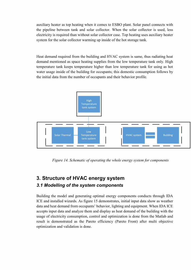
auxiliary heater as top heating when it comes to ESBO plant. Solar panel connects with
the pipeline between tank and solar collector. When the solar collector is used, less
electricity is required than without solar collector case. Top heating uses auxiliary heater
system for the solar collector warming up inside of the hot storage tank.
Heat demand required from the building and HVAC system is same, thus radiating heat
demand mentioned as space heating supplies from the low temperature tank only. High
temperature tank keeps temperature higher than low temperature tank for using as hot
water usage inside of the building for occupants; this domestic consumption follows by
the initial data from the number of occupants and their behavior profile.
High Temperature tank system
Low Temperature tank system
HVAC system BuildingSolar Thermal
Figure 14. Schematic of operating the whole energy system for components
3. Structure of HVAC energy system
3.1 Modelling of the system components
Building the model and generating optimal energy components conducts through IDA
ICE and installed wizards. As figure 15 demonstrates, initial input data show as weather
data and heat demand from occupants’ behavior, lighting and equipment. When IDA ICE
accepts input data and analyze them and display as heat demand of the building with the
usage of electricity consumption, control and optimization is done from the Matlab and
result is demonstrated as the Pareto efficiency (Pareto Front) after multi objective
optimization and validation is done.

Weather data
Energy simulation analysis (IDA ICE)
Occupantsbehavior
Light
Euqipment
Optimal chanrging schedule
(low temperature tank / solar collector)
Optimizing size of thermal tanks and
solar collectorValidation
Space heating Heat demand
Domestic hot water
Heat demand
Heat demand
Cost saving
Figure 15. Work process with simulation and optimizing software
This study is based on fulfilling the energy demand of residential single-family house
with two-story house. It assumes that building is generally considered to be connected
two-ground source heat pump models with solar collector and Air Handling Unit (AHU)
to ventilate the whole building envelop. For warming up the building envelope, two
geothermal heat pumps connect separately to each thermal tank. One thermal tank uses
for space heating and connected to the AHU for radiator system. Another thermal tank
employs to use hot water inside of the building. In Finnish building, hot water uses for
making the building warm and following the occupants’ usage profile. The former
thermal tank is applied to the preheating and useful for the radiation system for the
building envelope. Radiating the building envelope inside requires different heat demand
by the building type, massive passive, medium and lightweight.
AHU lets the inside of single family house warm up as space heating method and keeps
temperature as 21°C satisfying heating demand of the inside building depending on
occupancy behaviors and outdoor temperature. Hot temperature tank connects with heat
pump model 1 and sends domestic hot water into the building while preheating tank plugs
into the heat pump 2. Low temperature tank connects with solar collector and AHU
separately and high temperature tank works for offering domestic hot water in the
building by the schedule. Temperature control conducts through the whole system
connected to the building and valve and water flow control is dependent on the
temperature control in each case. Figure 16 explains the temperature control for the low
temperature tank with solar thermal, high temperature tank and air handling unit with
building cases.
HEAT Pump 1
SolarCollector
BuildingLT
HT
LT Te
To
TsTi
Cold water(7˚C )
TwinTwout
HEAT Pump 2
75˚C
55˚C
35˚C
55˚C
40˚C
50˚C
45˚C
60˚C
55˚C
30˚C40˚C
21˚C
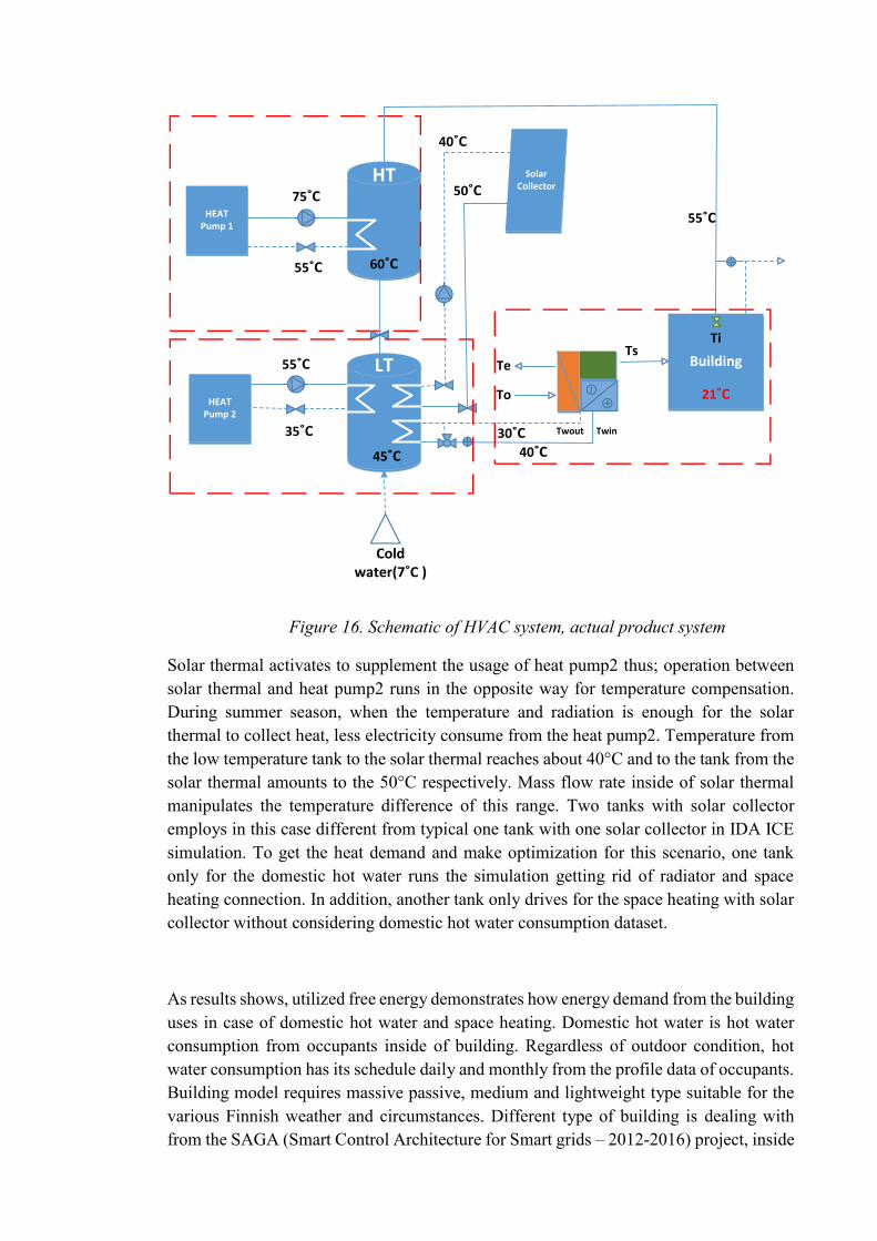
Figure 16. Schematic of HVAC system, actual product system
Solar thermal activates to supplement the usage of heat pump2 thus; operation between
solar thermal and heat pump2 runs in the opposite way for temperature compensation.
During summer season, when the temperature and radiation is enough for the solar
thermal to collect heat, less electricity consume from the heat pump2. Temperature from
the low temperature tank to the solar thermal reaches about 40°C and to the tank from the
solar thermal amounts to the 50°C respectively. Mass flow rate inside of solar thermal
manipulates the temperature difference of this range. Two tanks with solar collector
employs in this case different from typical one tank with one solar collector in IDA ICE
simulation. To get the heat demand and make optimization for this scenario, one tank
only for the domestic hot water runs the simulation getting rid of radiator and space
heating connection. In addition, another tank only drives for the space heating with solar
collector without considering domestic hot water consumption dataset.
As results shows, utilized free energy demonstrates how energy demand from the building
uses in case of domestic hot water and space heating. Domestic hot water is hot water
consumption from occupants inside of building. Regardless of outdoor condition, hot
water consumption has its schedule daily and monthly from the profile data of occupants.
Building model requires massive passive, medium and lightweight type suitable for the
various Finnish weather and circumstances. Different type of building is dealing with
from the SAGA (Smart Control Architecture for Smart grids – 2012-2016) project, inside
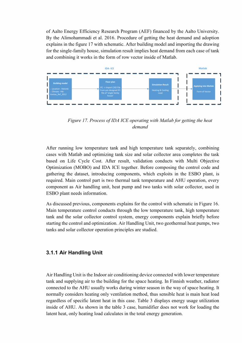
of Aalto Energy Efficiency Research Program (AEF) financed by the Aalto University.
By the Alimohammadi et al. 2016. Procedure of getting the heat demand and adoption
explains in the figure 17 with schematic. After building model and importing the drawing
for the single-family house, simulation result implies heat demand from each case of tank
and combining it works in the form of row vector inside of Matlab.
Building model
-. Location : Helsinki-. Climate : Hki- Vantaa_Ref_2012
Floor plan
IFC -> Import CAD FileFrom pre designed IFC
file of ’single family house’
Simulation Result
Heating & Cooling Load
Applying into Matlab
Form of Vector
IDA- ICE Matlab
Figure 17. Process of IDA ICE operating with Matlab for getting the heat
demand
After running low temperature tank and high temperature tank separately, combining
cases with Matlab and optimizing tank size and solar collector area completes the task
based on Life Cycle Cost. After result, validation conducts with Multi Objective
Optimization (MOBO) and IDA ICE together. Before composing the control code and
gathering the dataset, introducing components, which exploits in the ESBO plant, is
required. Main control part is two thermal tank temperature and AHU operation, every
component as Air handling unit, heat pump and two tanks with solar collector, used in
ESBO plant needs information.
As discussed previous, components explains for the control with schematic in Figure 16.
Main temperature control conducts through the low temperature tank, high temperature
tank and the solar collector control system, energy components explain briefly before
starting the control and optimization. Air Handling Unit, two geothermal heat pumps, two
tanks and solar collector operation principles are studied.
3.1.1 Air Handling Unit
Air Handling Unit is the Indoor air conditioning device connected with lower temperature
tank and supplying air to the building for the space heating. In Finnish weather, radiator
connected to the AHU usually works during winter season in the way of space heating. It
normally considers heating only ventilation method, thus sensible heat is main heat load
regardless of specific latent heat in this case. Table 3 displays energy usage utilization
inside of AHU. As shown in the table 3 case, humidifier does not work for loading the
latent heat, only heating load calculates in the total energy generation.

Table 3. Energy generation inside of Air Handling Unit
The structure of air handling unit demonstrates in figure 18. This AHU is two-floored
AHU with heat recovery system for the higher energy efficiency. Usually AHU has
supply and return fan, humidifier, filter, motor to operate, heating and cooling coil for
energy transfer. When the rotary heat recovery implies into the AHU, AHU saves energy
and becomes more economical than normal one floored type. Heat recovery adopts the
enthalpy transfer method considering sensible and latent heat together passing the airflow
through the air-handling unit. Moisturized Asian countries accept sensible and latent heat
recovery; this study only considers sensible heat load for the AHU operation.
Figure 18. Inner structure of Air Handling Unit
AHU regards to connect with the radiating system in the room and low temperature tank
in the system together. When low temperature tank reaches the temperature 45°C, it
supplies water to the AHU opening the 3-way valve and temperature from the AHU

receives energy and transfers it to the building envelope supplying the airflow. This
describes in figure 19.
AHUTwin
Twout 30˚C
40˚C
LT
Figure 19. Air Handling Unit temperature variation from and to the tank model
In the view of heating mode energy generation, AHU does not consider the moisturized
energy transfer; sensible heat demand equation completes in this research. Efficiency of
AHU demonstrates depending on the temperature of inlet and outlet from the AHU.
ηAHU = (Twin – Twout) / (Twin- Ta1) (12)
where
ηAHU Efficiency of AHU
𝑇𝑤𝑖𝑛 Supply air temperature of AHU
𝑇𝑤𝑜𝑢𝑡 Exhaust air temperature of AHU
Ta1 Temperature inside of AHU coil
𝐺𝑣𝑒𝑛 Thermal capacity of ventilation (W/K)
Thermal conductance of ventilation is depending on mass flow, density and air capacity.
Gven = ms ∗ρ*Cp (13)
where
ms Mass flow of air
ρ Density of air
C Specific heat capacity of air

Heat demand from the AHU only considers sensible heat requirement of the room in the
building model. Written again, this room is heating only. Energy balance for room
calculates based on the sensible energy balance formulae.
Qroom_sensible = msC ∗(Tr − Ts) (14)
where
Tr Room Temperature
Ts Surface temperature
ms Mass flow of air
C Specific air capacity
When mixing box used, temperature for the mixing box decides depending on the outdoor
temperature and room temperature.
Tmix = (1 − r)To + rTr (15)
where
r Mixing ratio
Tmix Temperature in the mixing box
To Outdoor temperature
Tr Room Temperature
Energy balance for heating coil shows by the mixing temperature and surface
temperature.
QHeating = msCp(Ts − TM) (16)
When the indoor temperature retains as 21°C constant, heat load from the AHU displays
formulae as this.
ΦAHU=Gven*(Ts-(To+ηAHU*(Ti-To))) (17)
When it adopts to use IDA simulation software, set point temperature of AHU is 18°C
for the constant building temperature as figure 20. This is default value and can
manipulate manually. Temperature inside of AHU with the outdoor temperature, AHU

air flows and energy generation checks in the IDA simulation. Cooling and heating coil
turn on and off by the usage of measuring in case of sensible heat and latent heat demand.
Figure 20. Set point temperature and connection inside of AHU
Heat demand from AHU is same as the room heat demand in the building envelope when
it uses radiator as discussed previous model.
3.1.2 Ground Source Heat Pump
Heat pump is the device to transfer heat from absorbing at the heat source to the heat sink
spontaneously. Reversed Carnot cycle (Refrigeration Cycle) uses to explain the heat
pump similar as the air conditioning model. In the Mollier diagram, so called P-H
(Pressure - Enthalpy) diagram, heat pump absorbs energy from the evaporator and loses
energy in the heat sink generally called condenser. When heat absorption occurs
evaporator, electricity consumption happens with heat pump operation and heat sink
happens in the condensation. As the figure 21 demonstrates for the Refrigeration cycle,
p1 is the high pressure for condensation and p2 is the lower pressure for evaporation. Heat
is absorbed from a->b and work with compressor at b->c and condensation happens when
pressure achieves to the p1. d-> a is the process throttling and enthalpy is set as same.

This procedure is simple refrigeration cycle and air conditioning system applies to this.
However, for the HVAC system, usually heat pump considers to employ the refrigeration
cycle so called reversed Carnot achieves.
Figure 21. Refrigeration cycle with pressure and enthalpy
Four types of Heat pumps applies into the Finnish HVAC system. Ground source
(Geothermal), Air to water, exhaust air and air-to-air heat pumps are those. Most energy
efficient and highly electricity consumption saving and cost effective product is ground
source heat pump, although total investment cost for ground source heat pump requires
the most compared with other heat pump types. Table 4 from the SULPU (Finnish heat
pump association) in 2013 compares prices and saving electricity by the different types
of heat pump models.
Heat Pump
Type
Saving
kWh/a
Saving(1)
€ /a
Investment(2)
€
Ground Source 14 000 - 17 000 1 800 - 2 200 14 000 - 20 000
Air - Water 8 000 - 13 000 1 000 - 1 700 8 000 - 12 000
Exahust Air 3 000 - 7 000 400 - 800 6 000 - 10 000(3)
Air - Air 2 000 - 7 000 250 - 800 1 500 - 2 500
Table 4. Cost and energy saving by the heat pump types (by SULPU data in
2013)
In the table, savings and investment cost are determined and reference from price
explains.

1) Electricity and oil 0.13 €/kWh (electricity 13 c/kWh and oil 1.1 €/l with 80% annual
operating efficiency)
2) Investment cost including installation, excluding heat delivery system
3) Including ventilation device, excluding channel installations Explanation of GSHP and
two heat pump type connected separately.
According to the US EPA (United States Environmental Protection Agency), geothermal
heat pumps can reduce energy consumption up to 44% compared with air-source heat
pumps and up to 72% compared with electric resistance heating. Heat pump selects as the
energy efficient source and usually occupies 5 % of the whole energy system by the statics
of Finland, Finnish Energy association in 2013. Using higher energy efficient heat pump
contributes to the better thermal effectiveness of the system. This explains how the
geothermal heat pump selects to make the better energy saving system in this research.
Coefficient of performance in the low temperature tank decides by the ratio between the
heating power of the ground source heat pump and its electricity consumption as below
equation.
COPN = Qout
Welectric (18)
where
Qout Heating power of heat pump
Welectric Electricity consumption of heat pump
This measured COP is get from the one test point and this is assumed to be constant
throughout the entire experimental period (one year in the simulation), to adopt the dataset
inside simulation software, hourly theoretical COP is required.
Theoretical COP comes from the temperature difference inside of reverse Carnot cycle
and generally describes with temperature between the condenser and evaporator when it
uses single type heat pump not the cascade nor combined case. It explains maximum
Carnot COP or refrigeration COP as equation (27) presents by the Laitinen et al.(2014).
COPc(t) = Tcon
Tcon−Teva (19)

where
Tcon Condenser temperature (K)
Teva Evaporator temperature (K)
The hourly computed practical temperature difference for the ground source heat pump
of theoretical COPT defines as formulae (28) by one-hour time step.
COPT =THSy
THSy−THSo (20)
where
THSy Building heating system temperature, K
THSo Heating source temperature, K
In the geothermal heat pump, THSy studies as the temperature of the fluid leaving the heat
collection circuit and entering the evaporator and it usually computes with the hot tank
inlet and outlet temperature connected with the heat pump.
In this thesis, Coefficient of performance (COP) with ground source heat pump is
determined from the heat pump (Mitsubishi and Nibe) of SAGA (Smart Control
Architecture for Smart grids – 2012-2016) project by the Niemelä et al. 2015. Heat pumps
in general have the COP of 4.2 to 4.6, which places it behind cogeneration with a COP of
9. In the IDA ICE of this work, COP of 4 reciprocating geothermal heat pump is chosen
to link with thermal tanks.
3.1.3 High temperature storage tank
High temperature tank assumes to supply heat to the hot water consumption in the house.
It considers as high temperature tank and temperature range approaches from 55°C to
65°C. Tank is stratified fluid type with connecting domestic hot water pipe and heat pump
with electric heater. Figure 22 demonstrates the energy balance from the tank to the house
with heat balance schematic.

HT
Figure 22. Heat flow of the high temperature tank
When balance equation completes in the tank model, formulae is get from the Dwivedi et
al. in 2009.
��s*Cp*𝑑𝑇𝑠
𝑑𝑡 = Qheatpump1 – Qdomestic – U*A*(Ts-Ta) (21)
where
Qheatpump1 Heat power from the heat pump connected by the high
temperature tank
Qdomestic Heat load transferred to the hot water consumption
U Tank heat loss conductance (W/m2K).
A Area of the thermal tank (m2 )
Ts Instantaneous temperature of the tank (K)
Ta Ambient temperature of the tank (K)
ms Mass of water in the storage tank (kg)
CP Heat capacity of water (J/kg*K)
Heat pump generates the heat power regularly connected to the thermal tank system.
When the domestic hot water consumption load is satisfied, size of the hot water tank can
optimize depending on this equation.

3.1.4 Low temperature storage tank
Low temperature tank operates between the temperature 40°C and 50°C. It links with
high temperature tank, solar collector, ground source heat pump and AHU system for the
space heating. It is supposed to open the valve between the two thermal tanks and high
temperature tank receives water path when the temperature of low temperature tank reaches
around 45°C. Solar collector gathers solar radiation and temperature during the whole
year and lets the heat pump electricity consumption less to operate the low temperature
tank in the static condition for the accepted temperature range. Figure 23 demonstrates
the heat balance of the tank in schematic.
Figure 23. Heat balance of the low temperature tank
As figure shows, low temperature tank energy balance is dependent on the heat power
from the heatpump2, high temperature tank, solar collector and AHU. When it comes to
the formulae, equation (22) shows its relations.
��Low temperature tank = ��s*Cp*𝑑𝑇𝑠
𝑑𝑡 = ��heatpump2 + ��solar collector – U*A*(Ts-Ta) – ��AHU (22)
where
��Low temperature tank Heat power from the low temperature tank
��heatpump2 Heat power from the heat pump connected to the low
temperature tank

��solar collector Heat gain from the solar collector
��AHU Heat load transferred as radiation for space heating
U Tank heat loss conductance (W/m2K).
A Area of the thermal tank (m2 )
Ts Instantaneous temperature of the tank (K)
Ta Ambient temperature of the tank (K)
ms Mass of water in the storage tank (kg)
CP Heat capacity of water (J/kg*K)
In the low temperature tank model, heat loss in the tank is different by the time and it can
be get as iterative method by the hourly time step heat-demand data calculating as row
vector. Solar collector can reduce the electricity consumption of the heat pump and this
leads to the energy saving especially during the summer season.
3.1.5 Solar Collector
Solar collector is key component for the thermal tank system with solar heating. Solar
thermal transforms solar energy as radiation permeates into the heat in the liquid inside
of the collector. Generally, two main types of solar collector employs; Flat plate collectors
and concentrating collectors. In the flat plate collector, solar absorbing surface in the plate
is almost same size as the overall collector area, while concentrating collector employs
small area of collector with mirror reflection to gather the solar energy. In this thesis, flat
plate collector employs and it usually studies in the single-family house of the Finland.

Figure 24. Flat plate solar collector whole structure
Figure 24 explains the whole structure of flat plate solar collector with inlet and outlet
temperature with fluid. When the solar radiation (W/ m2) is absorbed to the flat plate of
solar thermal, solar thermal gathers it by the surface area of the collector (m2). When the
surface area of the collector receives it, transmittance coefficient through the glazing and
absorption coefficient for plate considers solar rays to let it arrive and penetrate into the
transparent cover of the collector. Collector heat input (��i) regards as equation (23).
��i = I(τ α)Ac (23)
where
I Solar radiation density to solar collectors (W/m2)
α Absorption coefficient of plate
τ Transmittance coefficient of glazing
Ac Collector area (m2)
As the solar thermal absorbs solar heat, temperature inside the collector raises higher than
the ambient temperature surrounded, it loses energy to the atmosphere as radiation and
convection heat load by the overall transfer coefficient. Useful energy gain (��u) from the
solar collector presents formulae (24) with the whole energy gained from the collector
and removal of this heat loss.
��u = ��i - ��o = I(τ α)Ac - UL(Tc – Ta) (24)
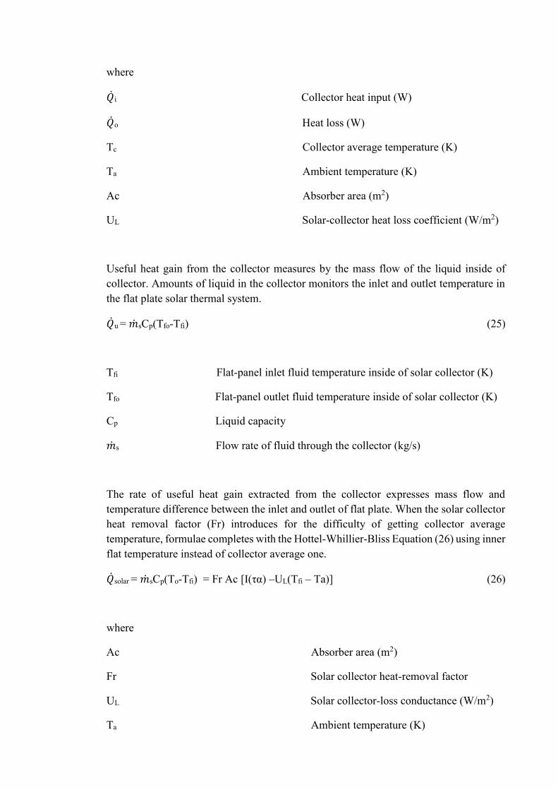
where
��i Collector heat input (W)
��o Heat loss (W)
Tc Collector average temperature (K)
Ta Ambient temperature (K)
Ac Absorber area (m2)
UL Solar-collector heat loss coefficient (W/m2)
Useful heat gain from the collector measures by the mass flow of the liquid inside of
collector. Amounts of liquid in the collector monitors the inlet and outlet temperature in
the flat plate solar thermal system.
��u = ��sCp(Tfo-Tfi) (25)
Tfi Flat-panel inlet fluid temperature inside of solar collector (K)
Tfo Flat-panel outlet fluid temperature inside of solar collector (K)
Cp Liquid capacity
��s Flow rate of fluid through the collector (kg/s)
The rate of useful heat gain extracted from the collector expresses mass flow and
temperature difference between the inlet and outlet of flat plate. When the solar collector
heat removal factor (Fr) introduces for the difficulty of getting collector average
temperature, formulae completes with the Hottel-Whillier-Bliss Equation (26) using inner
flat temperature instead of collector average one.
��solar = ��sCp(To-Tfi) = Fr Ac [I(τα) –UL(Tfi – Ta)] (26)
where
Ac Absorber area (m2)
Fr Solar collector heat-removal factor
UL Solar collector-loss conductance (W/m2)
Ta Ambient temperature (K)

Collector efficiency can describe with the ratio of the useful energy gain (��u) and the
incident solar energy reckoning time-period.
η = ∫ ��𝑢 d𝑡
𝐴 ∫ 𝐼 d𝑡 =
Fr Ac [I(τα) –UL(Tfi – Ta)]
𝐴𝐼 (27)
Hottel-Whillier-Bliss Equation employs the equation; it completes the formulae as (27).
To calculate steady state solar collector for useful energy, gain with function of fluid inlet
temperature and ambient temperature, mass flow rate of the water inside of collector is
key parameter. It is optimization decision variables for the higher efficiency of the whole
system. Solar collector works based on the demand of low temperature tank. When the
solar radiation is enough to load the heat gain into the thermal tank, minimum electricity
consumption is required in the heat pump model of the low temperature tank. Simulation
software generates the temperature-varying model in this case to generate the cost
effective model for controlling the system.
4. Control strategy method for energy system
4.1 Simulation Based Control system
Heat load requirement from the building model as space heating is depending on the
control of the low storage tank and solar collector response. Domestic hot water
consumption in the single-family house is based on the charging schedule of the hot water
tank. In the control point of view, control system requires three main components. Two
thermal tank models and control strategy between low temperature tank and solar
collector. Figure 25 expresses temperature control between two tanks.
When the temperature of the low storage tank exceeds the satisfying temperature of 45°C,
water flows to the high temperature tank until it approaches to the 60°C. Low temperature
tank and high temperature tank applies individual geothermal heat pump, it works based
on the heat demand of the tank system. To optimize the size of tanks and solar collector,
three models generates for control and optimization. The system with high temperature
tank only for domestic hot water consumption, system with low temperature tank only
with solar collector for space heating and the system with low temperature tank only
without solar collector system are included; those are named as split type models.

LT
40˚C<T<50˚C
HT
50˚C<T
SolarCollector
Figure 25. Control strategy between two tanks and solar collector
IDA simulation only generates the one tank with solar collector model, this split type
models combine after getting separate head demand from IDA simulation separately.
Massive, medium and light type of buildings are generated for domestic hot water only,
space heating only with solar collector and space heating only without solar collector. All
type of buildings’ control strategy completes with three split models.
From the formulae (21) and (22), high temperature tank ( ��High temperature tank) and low
temperature tank (��Low temperature tank) is equivalent with the ��domestic water only and �� space heating
only with solar respectively. Split type model is required for controlling the two tank models,
��High temperature tank considers only working for the hot water consumption and the ��Low
temperature tank is for space heating with solar collector system. Written again, formulae
completes with (28) and (29).
��High temperature tank = ��domestic water only = ��s*Cp*𝑑𝑇𝑠
𝑑𝑡 = Qheatpump1 – Qdomestic – U*A*(Ts-Ta)
(28)
��Low temperature tank = �� space heating only with solar = ��s*Cp*𝑑𝑇𝑠
𝑑𝑡 = ��heatpump2 + ��solar collector -
U*A*(Ts-Ta) - ��AHU (29)
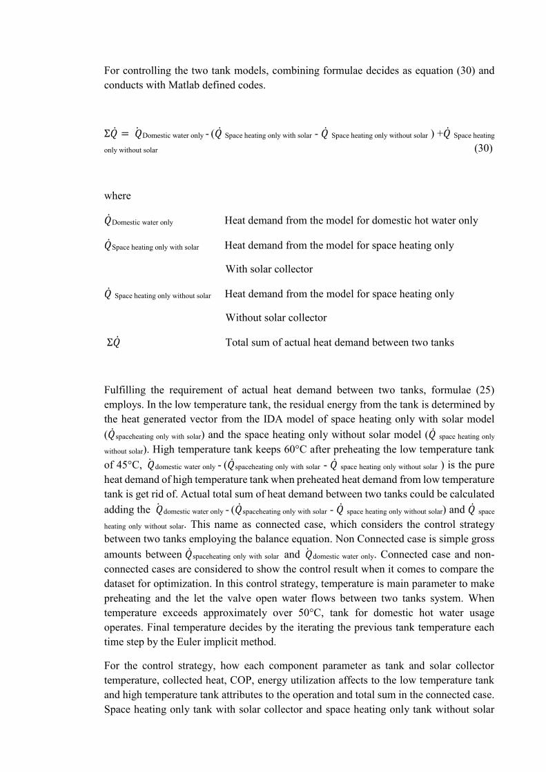
For controlling the two tank models, combining formulae decides as equation (30) and
conducts with Matlab defined codes.
Ʃ�� = ��Domestic water only - (𝑄 Space heating only with solar - �� Space heating only without solar ) +�� Space heating
only without solar (30)
where
��Domestic water only Heat demand from the model for domestic hot water only
��Space heating only with solar Heat demand from the model for space heating only
With solar collector
�� Space heating only without solar Heat demand from the model for space heating only
Without solar collector
Ʃ�� Total sum of actual heat demand between two tanks
Fulfilling the requirement of actual heat demand between two tanks, formulae (25)
employs. In the low temperature tank, the residual energy from the tank is determined by
the heat generated vector from the IDA model of space heating only with solar model
(��spaceheating only with solar) and the space heating only without solar model (�� space heating only
without solar). High temperature tank keeps 60°C after preheating the low temperature tank
of 45°C, ��domestic water only - (��spaceheating only with solar - �� space heating only without solar ) is the pure
heat demand of high temperature tank when preheated heat demand from low temperature
tank is get rid of. Actual total sum of heat demand between two tanks could be calculated
adding the ��domestic water only - (��spaceheating only with solar - �� space heating only without solar) and �� space
heating only without solar. This name as connected case, which considers the control strategy
between two tanks employing the balance equation. Non Connected case is simple gross
amounts between ��spaceheating only with solar and ��domestic water only. Connected case and non-
connected cases are considered to show the control result when it comes to compare the
dataset for optimization. In this control strategy, temperature is main parameter to make
preheating and the let the valve open water flows between two tanks system. When
temperature exceeds approximately over 50°C, tank for domestic hot water usage
operates. Final temperature decides by the iterating the previous tank temperature each
time step by the Euler implicit method.
For the control strategy, how each component parameter as tank and solar collector
temperature, collected heat, COP, energy utilization affects to the low temperature tank
and high temperature tank attributes to the operation and total sum in the connected case.
Space heating only tank with solar collector and space heating only tank without solar

collector is considered as low temperature tank control, domestic hot water only tank is
high temperature tank control and the last, control between solar collector and low
temperature tank shall be explained.
4.1.1 Low temperature storage tank control
Low-temperature tank control has two simulation models. One is space heating only tank
model with solar collector and the other is space heating only tank model without solar
collector. For setting up, in the IDA ICE ESBO plant, getting rid of connection pipe of
domestic hot water usage and setting schedule of domestic hot water consumption profile
as zero value is main task. For the space heating only with solar collector model in figure
26, solar collector setting temperature is dependent on the PI control and it manipulates
as 5°C. In addition, the thermostat temperature for the variable set point, it decides as 95
°C as maximum.
Figure 26. Space heating only tank with solar collector model

In case of the space heating only without solar collector model in figure 27, solar collector
pipe connection deletes as red box shows. In addition, domestic hot water consumption
usage is not available same as Figure 26.
Figure 27. Space heating only tank without solar collector model
Figure 28 is the ground heat exchanger in the ESBO plant, adopting borehole and pipe
type. As presented, heat exchanger directly links to the ground source heat pump and
mass flow, thus heat collected in the exchanger is object to the heat pump power operation
and working hour. Space- heating only with solar collector or without solar collector
model demonstrates energy generation and mass flow in the result section to show the
correlation with heat pump operation.
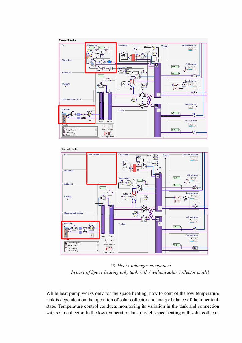
28. Heat exchanger component
In case of Space heating only tank with / without solar collector model
While heat pump works only for the space heating, how to control the low temperature
tank is dependent on the operation of solar collector and energy balance of the inner tank
state. Temperature control conducts monitoring its variation in the tank and connection
with solar collector. In the low temperature tank model, space heating with solar collector

and space heating without solar collector samples gather separately in massive medium
and light building models; tank size changes from 0.5 m3 to 2 m3 , solar collector area
comes from 1 m2 to 10 m2. Thus, 40 samples for space heating with solar collector and 4
samples for solar collector without solar collector model. Three different building
insulation types are included, 132 samples generate for control strategy and optimization
later on.
4.1.2 High temperature storage tank control
High temperature tank only works for the hot water consumption. From the normal IDA
one tank simulation, getting rid of space heating radiator and AHU is essential to generate
the domestic hot water only model. From the whole envelope of the building model,
central Air handling unit deletes blocking to offer the radiation into the building as figure
29 shows.
Figure 29. Insulation of the whole spaces and domestic hot water only model
generation
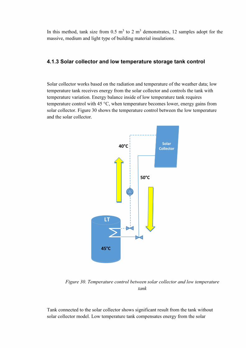
In this method, tank size from 0.5 m3 to 2 m3 demonstrates, 12 samples adopt for the
massive, medium and light type of building material insulations.
4.1.3 Solar collector and low temperature storage tank control
Solar collector works based on the radiation and temperature of the weather data; low
temperature tank receives energy from the solar collector and controls the tank with
temperature variation. Energy balance inside of low temperature tank requires
temperature control with 45 °C, when temperature becomes lower, energy gains from
solar collector. Figure 30 shows the temperature control between the low temperature
and the solar collector.
SolarCollector
LT
40°C
50°C
45°C
Figure 30. Temperature control between solar collector and low temperature
tank
Tank connected to the solar collector shows significant result from the tank without
solar collector model. Low temperature tank compensates energy from the solar
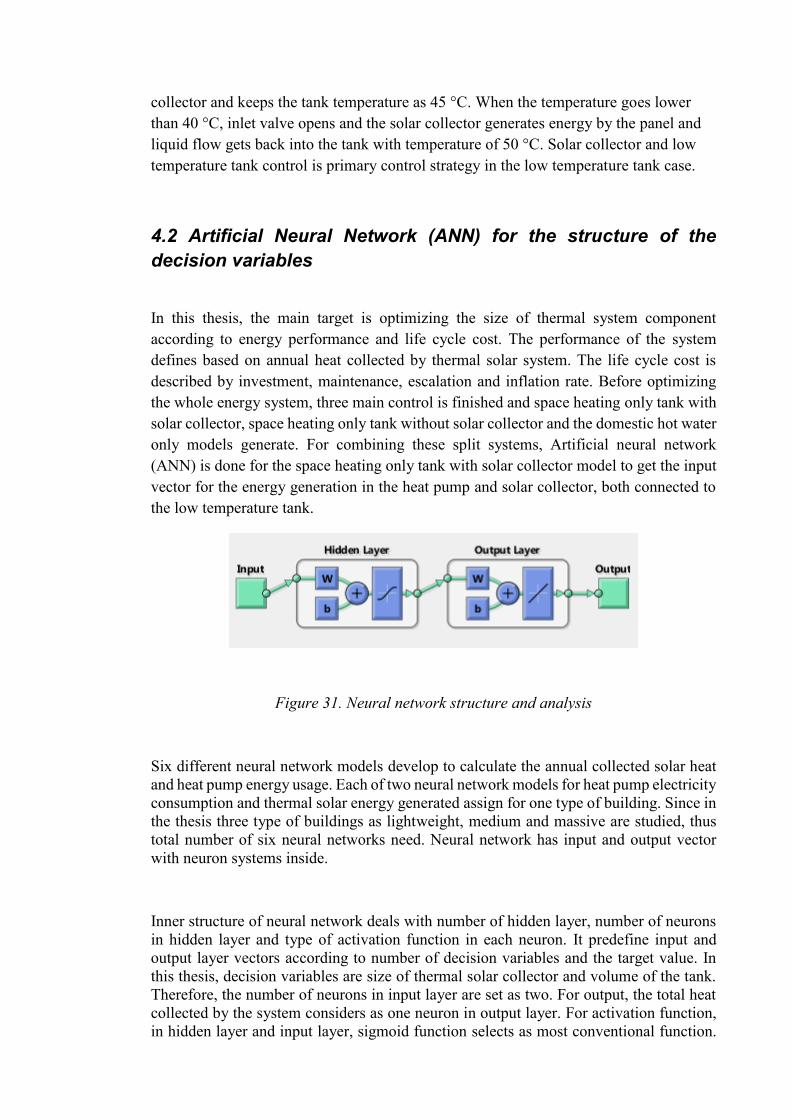
collector and keeps the tank temperature as 45 °C. When the temperature goes lower
than 40 °C, inlet valve opens and the solar collector generates energy by the panel and
liquid flow gets back into the tank with temperature of 50 °C. Solar collector and low
temperature tank control is primary control strategy in the low temperature tank case.
4.2 Artificial Neural Network (ANN) for the structure of the
decision variables
In this thesis, the main target is optimizing the size of thermal system component
according to energy performance and life cycle cost. The performance of the system
defines based on annual heat collected by thermal solar system. The life cycle cost is
described by investment, maintenance, escalation and inflation rate. Before optimizing
the whole energy system, three main control is finished and space heating only tank with
solar collector, space heating only tank without solar collector and the domestic hot water
only models generate. For combining these split systems, Artificial neural network
(ANN) is done for the space heating only tank with solar collector model to get the input
vector for the energy generation in the heat pump and solar collector, both connected to
the low temperature tank.
Figure 31. Neural network structure and analysis
Six different neural network models develop to calculate the annual collected solar heat
and heat pump energy usage. Each of two neural network models for heat pump electricity
consumption and thermal solar energy generated assign for one type of building. Since in
the thesis three type of buildings as lightweight, medium and massive are studied, thus
total number of six neural networks need. Neural network has input and output vector
with neuron systems inside.
Inner structure of neural network deals with number of hidden layer, number of neurons
in hidden layer and type of activation function in each neuron. It predefine input and
output layer vectors according to number of decision variables and the target value. In
this thesis, decision variables are size of thermal solar collector and volume of the tank.
Therefore, the number of neurons in input layer are set as two. For output, the total heat
collected by the system considers as one neuron in output layer. For activation function,
in hidden layer and input layer, sigmoid function selects as most conventional function.

In output layer, sign function form the results of neural network. The main task for finding
the right structure of neural network does not have specific rule. The number of hidden
layer and corresponding neurons define with try and error process following the
Levenberg–Marquardt algorithm (LMA). It means it checks different number of hidden
layer and neurons with training data set and that structure which gives the lowest shall
select as final structure.
Network initializes by setting all its weights to be random number between -1 and +1.
Forward pass calculation processes from the target to get the actual value. Error of each
neuron is essentially Target – Actual Output. This error is then mathematically to change
the weight and bias in such way that error goes smaller. The error of network evaluates
with mean square error and correlation between output and reference data. The mean
square error deals with general accuracy of model and correlation describes how the
output and reference data have similar trend. For instance, correlation 0 means no
correlation and 1 means high performance of model. Training data set in this thesis
include 40 samples for each type of building in the space heating only tank with solar
collector model case. 70% of training data set is used in training and the rest of 15% each
samples are implemented in validation and testing the model.
Figure 32 demonstrates how IDA simulates energy generation and artificial neural
network operates for the parameters of heat pump and solar collector. Obtaining the
utilized energy from the IDA simulation and applies to the form of input layer inside of
ANN contributes to make the new structure for the optimization (NSGAII) in the scope
of the suitable solutions in decision variables.

Solar collector
Heat pump
Energy Generation (IDA-ICE)
Solar collector
Heat pump
ArtificialNeural Network
( Matlab)
NSGAII
Reference data Training the ANN models
Life cycle cost calculation
Optimal solutions
Fitness function 1
Fitness function 2
Figure 32. How ANN works based on IDA and Matlab
Contribution to the Multi objective optimization
Fitness function from the ANN and function from the Life Cycle Cost (LCC) decides as
the objective functions to organize the multi objective optimization. From the whole 144
samples considering light, medium and massive building type, each type of building
model generates 48 samples as discussed previous. Domestic hot water only tank has 4
samples (Tank size : 0.5m3, 1m3, 1.5m3, 2m3), space heating only without solar collector
also gets 4 (Tank size : 0.5m3, 1m3, 1.5m3, 2m3), while space heating only model with
solar collector produces 40 samples (4 tank samples with 10 amounts of solar collector
area). ANN structure is studied for the space heating only tank with solar collector using
the IDA simulation, as the reference data for other datasets are simple except of space
heating only with solar collector tank models.
5. Cost optimal solution method in energy building
Deciding the fitness functions to get the optimal size of solar collector and tank relates
with the Life Cycle Cost (LCC) of components and less electricity consumption in the
geothermal heat pumps. Cost of components and electricity usage in the heat pumps
work as objective functions respectively inside of optimization in the way of Non
Sorting Genetic Algorithm II (NSGA II). The definition of life cycle cost and the multi-

objective optimization methods are studied and the result comes out with the coded
Matlab software.
5.1 General explanation of Life Cycle Cost
For life cycle cost (LCC) analysis the main parameter considers as investment cost,
maintenance cost and profit from energy. The life span for the LCC analysis defines as
20 years so no cost for renovation assigns. The main components for LCC calculation are
hot water storage tank and thermal solar panel. The prices of these components extracts
based on Finnish market data. The price for thermal solar collector includes cost of
installation, panel, pump, pipes, control system and expansion chamber. The price for hot
water storage tank covers the installation, tank and heat exchangers. The required
parameters for LCC analysis presents in table 7. These parameters are interest rate and
inflation factor. Based on mentioned factors the following parameters computes with
below formulae.
Real interest rate calculates by equation (31).
( )
(1 )
i fr
f
(31)
where
i Nominal interest rate
f Inflation rate
Escalated real interest rate presents by equation (32).
( )
(1 )e
r er
e
(32)
where
r Real interest rate
e Escalation rate
Present value factor of annual maintenance cost defines by equation (33).
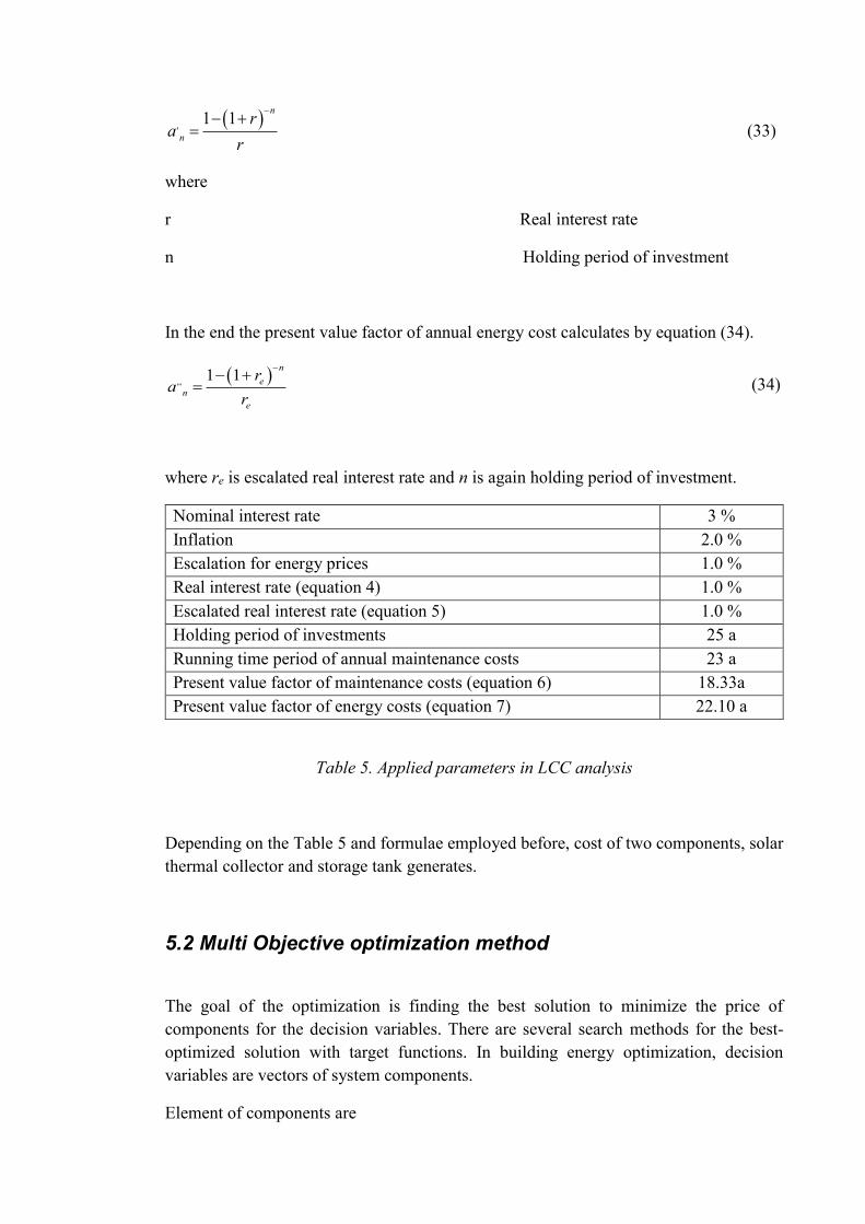
,1 1
n
n
ra
r
(33)
where
r Real interest rate
n Holding period of investment
In the end the present value factor of annual energy cost calculates by equation (34).
,,1 1
n
e
n
e
ra
r
(34)
where re is escalated real interest rate and n is again holding period of investment.
Nominal interest rate 3 %
Inflation 2.0 %
Escalation for energy prices 1.0 %
Real interest rate (equation 4) 1.0 %
Escalated real interest rate (equation 5) 1.0 %
Holding period of investments 25 a
Running time period of annual maintenance costs 23 a
Present value factor of maintenance costs (equation 6) 18.33a
Present value factor of energy costs (equation 7) 22.10 a
Table 5. Applied parameters in LCC analysis
Depending on the Table 5 and formulae employed before, cost of two components, solar
thermal collector and storage tank generates.
5.2 Multi Objective optimization method
The goal of the optimization is finding the best solution to minimize the price of
components for the decision variables. There are several search methods for the best-
optimized solution with target functions. In building energy optimization, decision
variables are vectors of system components.
Element of components are
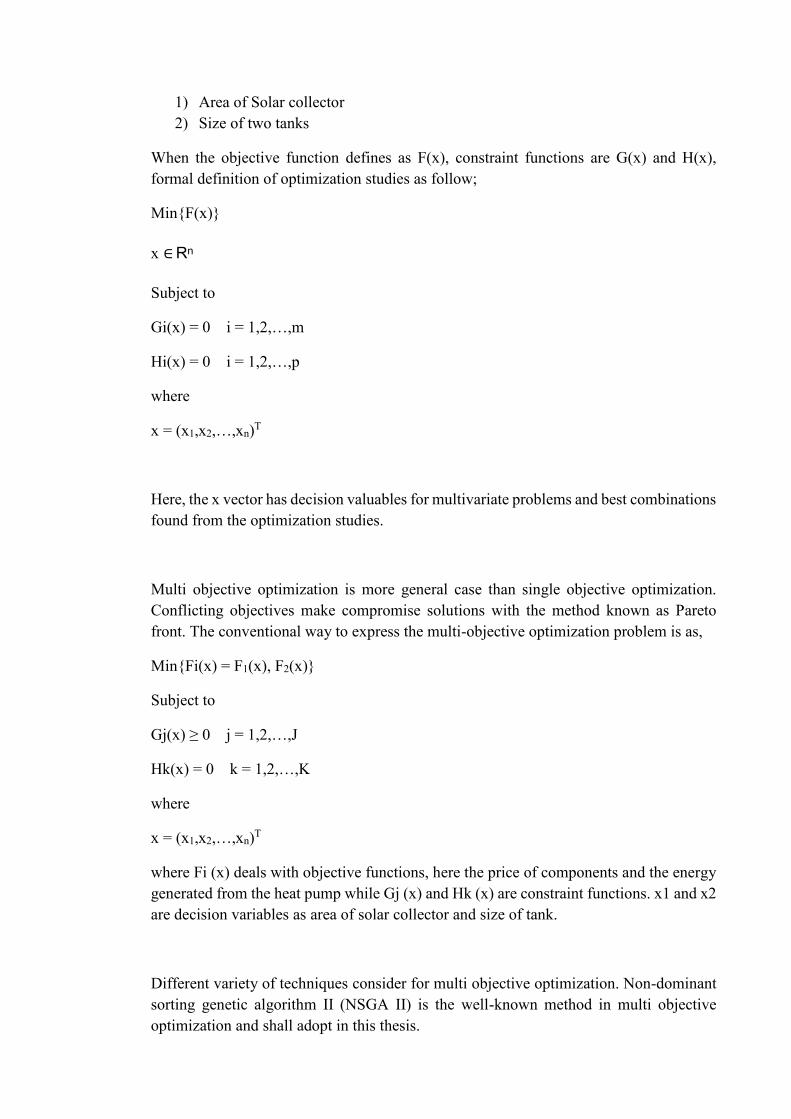
1) Area of Solar collector
2) Size of two tanks
When the objective function defines as F(x), constraint functions are G(x) and H(x),
formal definition of optimization studies as follow;
Min{F(x)}
x ∈ Rn
Subject to
Gi(x) = 0 i = 1,2,…,m
Hi(x) = 0 i = 1,2,…,p
where
x = (x1,x2,…,xn)T
Here, the x vector has decision valuables for multivariate problems and best combinations
found from the optimization studies.
Multi objective optimization is more general case than single objective optimization.
Conflicting objectives make compromise solutions with the method known as Pareto
front. The conventional way to express the multi-objective optimization problem is as,
Min{Fi(x) = F1(x), F2(x)}
Subject to
Gj(x) ≥ 0 j = 1,2,…,J
Hk(x) = 0 k = 1,2,…,K
where
x = (x1,x2,…,xn)T
where Fi (x) deals with objective functions, here the price of components and the energy
generated from the heat pump while Gj (x) and Hk (x) are constraint functions. x1 and x2
are decision variables as area of solar collector and size of tank.
Different variety of techniques consider for multi objective optimization. Non-dominant
sorting genetic algorithm II (NSGA II) is the well-known method in multi objective
optimization and shall adopt in this thesis.

5.2.1 Non Dominant Sorting Genetic Algorithm II (NSGA II)
The genetic algorithm (GA) is a search technique used in computing to find true or
approximate solution for optimization and search problems. GA categorizes as global
search heuristics. GA is a particular class of evolutionary algorithm that use techniques
inspired by evolutionary biology such as inheritance, mutation, selection, and crossover
(also called recombination). The evolution usually starts from a population of randomly
generated individuals and happens in generations. In each generation, the fitness function
of every individual in the population evaluates and multiple individuals selects from the
current population and modifies to form a new population. The new population uses in
the next iteration of the algorithm. The algorithm terminates when either a maximum
number of generations has produced, or a satisfactory fitness level has reached for the
population.
GA name indeed is an emphasis on motivation of genetic optimization algorithm based
on improving the individuals by manipulating of their genotype. GA is one of the most
popular technique in evolutionary computation research. In genetic algorithm the
candidate solution is presented as string and each position in the string is considered to
represent a particular feature of an individual. In better words, the value stored in that
position represents how that feature is expressed in the solution. Thus, variation of the
members of the string are expected to improve the solution. The changes in candidates is
applied by means of cross over and mutation. In cross over two strings are used as parents
and new individuals are formed by swapping a sub-sequence between the two strings
while in mutation the single member of the string is replaced with new one as figure 33.

Figure 33. Crossover and mutation operators in Genetic Algorithm
(From PHP coded site about GA, www.abrandao.com)
By applying these operators, great variety develops to solve design optimization problems
including discrete design parameters and then real parameter optimization problems. In
genetic algorithm after defining number of variables (number of cells in solution strings)
and determining the upper and lower boundaries for each variable, number of members
in population defines. Then for two main operators as cross over and mutation, the
percentage of probability describes to show how often each operators shall perform.
There are two basic parameters of GA as crossover probability and mutation probability.
If there is no crossover, offspring is exact copy of parents. If there is a crossover, offspring
makes from parts of parents' chromosome. The crossover probability could vary from
100%, which means all offspring makes by crossover to 0%, which means whole new
generation makes from exact copies of chromosomes from old population. In terms of
mutation if mutation probability assigns as 100%, whole chromosome changes, if it
defines as 0%, then nothing is changed. Mutation should prevent the changing of
procedure of GA into local extreme.
NSGAII extends version of genetic algorithm for multi objective problems. This method
uses the same tools for improving the population in each generation as cross over and
mutation. Nevertheless, in NSGAII two new concept applies to handle multi objective
problems. The first one is non-dominated sorting which based on given ranking to each
member of population defined non-dominated members. The next one is crowding
distance, which in simple word defines the distance between optimal solutions in Pareto
front to cover as much as possible as all optimal search space. These two concepts show
in figure 34.

Figure 34. Application of crowding distance and non-dominant sorting in NSGAII
In Figure 34, the black nodes are the set of non-dominated members of the ongoing
generation. It means that in compared with white nodes; black nodes have better value in
both defined objective functions. Also by using the crowding distance, the density of best
solution (black nodes) are defined in the way that solutions are located in proper distance
and cover all Pareto region.
6. Validation and Discussion
Control strategy and optimization conducts with two tank models with two heat pumps.
Before getting the result dataset, validating the model with one tank simulation with
optimization software is required. Two neural networks train with simulation based on
IDA ICE medium type of building in the one tank model at ESBO plant. The multi
objective optimization carries out by using these neural networks to find the set of optimal
solutions. The achieved results compare with multi objective optimization with using the
IDA-ICE and MOBO (Palonen et.al. 2013).
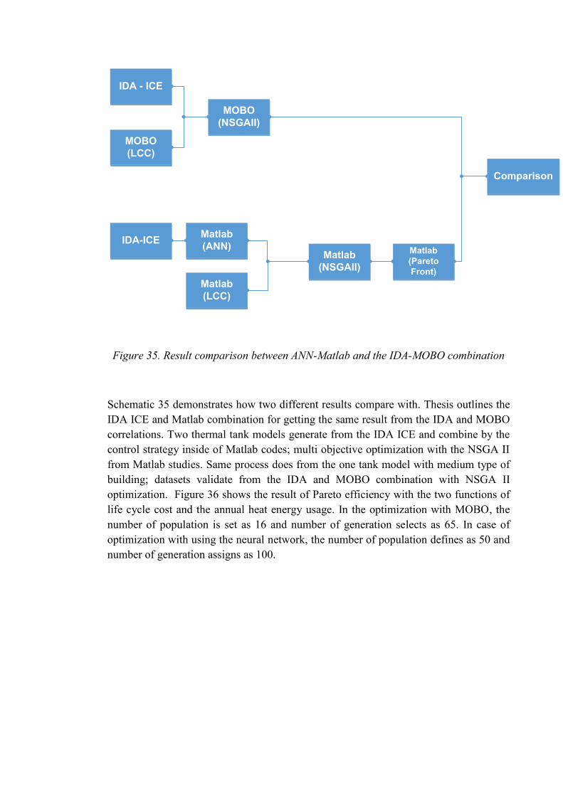
IDA - ICE
MOBO
(LCC)
MOBO
(NSGAII)
IDA-ICEMatlab
(ANN)
Matlab
(LCC)
Matlab
(NSGAII)
Matlab
(Pareto
Front)
Comparison
Figure 35. Result comparison between ANN-Matlab and the IDA-MOBO combination
Schematic 35 demonstrates how two different results compare with. Thesis outlines the
IDA ICE and Matlab combination for getting the same result from the IDA and MOBO
correlations. Two thermal tank models generate from the IDA ICE and combine by the
control strategy inside of Matlab codes; multi objective optimization with the NSGA II
from Matlab studies. Same process does from the one tank model with medium type of
building; datasets validate from the IDA and MOBO combination with NSGA II
optimization. Figure 36 shows the result of Pareto efficiency with the two functions of
life cycle cost and the annual heat energy usage. In the optimization with MOBO, the
number of population is set as 16 and number of generation selects as 65. In case of
optimization with using the neural network, the number of population defines as 50 and
number of generation assigns as 100.

Figure 36. Pareto Front result comparison between the ANN-Matlab and MOBO-IDA
Pattern between two methods correspond in the same pace, the suggested method is
reliable for finding the optimal solution.
7. Result
Generating the space heating only tank with solar collector, space heating only without
solar collector and domestic hot water models adopt to the artificial neural network and
optimization. Optimization result studies with Non Sorting dominant genetic algorithm
method using multi- objective optimization case. Cost of the solar collector and heat
pumps decides by the Life Cycle Cost (LCC) function and the energy generation of heat
pump usage compares for the optimal selection of the suitable tank. Furthermore, solar
collector sizes decide by the Pareto efficiency curve. When solar collector compensates
the heat pump usage, energy utilization inside of heat pump shrinks to the minimum.
The goal of this thesis is satisfying the two objective functions mentioned above. NSGA
II uses dataset from the artificial neural network (ANN) and control code defined for
connecting low temperature and high temperature tank. Influence of economic
parameter as interest rate changes from 3% to 9% when it comes to the LCC calculation
and plotting.

7.1 Control strategy result
Simulation employs two-tank system connected into the heat pumps separately. Usually,
normal one tank model shows temperature variation as figure 37. There are 8 layers inside
of tank and 1st layer at the bottom of the tank (figure 38) is connected to the space heating
temperature for the radiating the building envelope. 8th layered temperature inside of
stratified tank (figure 39) is used for the domestic hot water consumption of the house. It
is generally higher than the temperature for space heating.
Figure 37. Temperature variation inside of stratified tank

Figure 38. Temperature variation for 1st layer of hot storage tank
Figure 39. Temperature variation for 8th layer of hot storage tank

Figure 38 and 39 demonstrates temperature control happens when the low temperature
tank reaches 45°C and the high temperature tank approaches to the 60°C. Space heating
only with solar collector, space heating only without solar collector and domestic hot
water only models show different states when low temperature and high temperature
tank is applied.
7.1.1 The result of low temperature tank control strategy
Low-temperature tank links with the solar collector and AHU together for radiating
building envelope and getting compensate energy from the solar collector. Air handling
unit keeps the temperature of the room as 21°C constantly, thus the thermal comfort for
occupants’ behavior depends on heating load temperature satisfaction. To make the room
temperature constant, supply air maintains the specific temperature value inside of AHU.
Figure 40 shows how the supply air temperature is keeping stable when outdoor and
return air to the AHU fluctuates by the year.
Figure 40. Temperature variation of return and supply air inside of AHU
Depending on outdoor temperature
By the different outdoor temperature, inner building temperature should retain constant
all the time thus radiators inside of room in the building maintains energy balance with
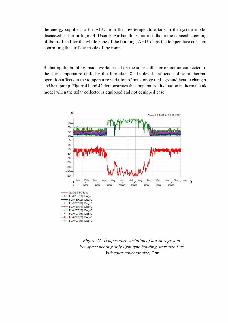
the energy supplied to the AHU from the low temperature tank in the system model
discussed earlier in figure 4. Usually Air handling unit installs on the concealed ceiling
of the roof and for the whole zone of the building, AHU keeps the temperature constant
controlling the air flow inside of the room.
Radiating the building inside works based on the solar collector operation connected to
the low temperature tank, by the formulae (8). In detail, influence of solar thermal
operation affects to the temperature variation of hot storage tank, ground heat exchanger
and heat pump. Figure 41 and 42 demonstrates the temperature fluctuation in thermal tank
model when the solar collector is equipped and not equipped case.
Figure 41. Temperature variation of hot storage tank
For space heating only light type building, tank size 1 m3
With solar collector size, 7 m2
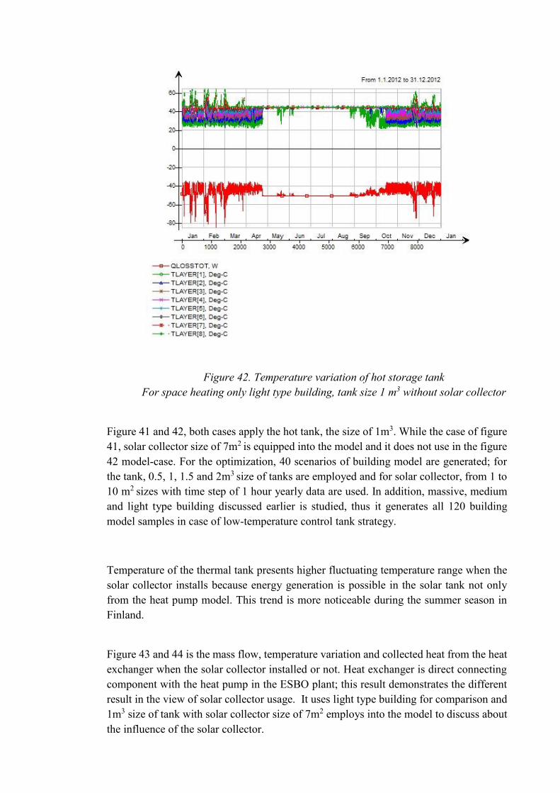
Figure 42. Temperature variation of hot storage tank
For space heating only light type building, tank size 1 m3 without solar collector
Figure 41 and 42, both cases apply the hot tank, the size of 1m3. While the case of figure
41, solar collector size of 7m2 is equipped into the model and it does not use in the figure
42 model-case. For the optimization, 40 scenarios of building model are generated; for
the tank, 0.5, 1, 1.5 and 2m3 size of tanks are employed and for solar collector, from 1 to
10 m2 sizes with time step of 1 hour yearly data are used. In addition, massive, medium
and light type building discussed earlier is studied, thus it generates all 120 building
model samples in case of low-temperature control tank strategy.
Temperature of the thermal tank presents higher fluctuating temperature range when the
solar collector installs because energy generation is possible in the solar tank not only
from the heat pump model. This trend is more noticeable during the summer season in
Finland.
Figure 43 and 44 is the mass flow, temperature variation and collected heat from the heat
exchanger when the solar collector installed or not. Heat exchanger is direct connecting
component with the heat pump in the ESBO plant; this result demonstrates the different
result in the view of solar collector usage. It uses light type building for comparison and
1m3 size of tank with solar collector size of 7m2 employs into the model to discuss about
the influence of the solar collector.
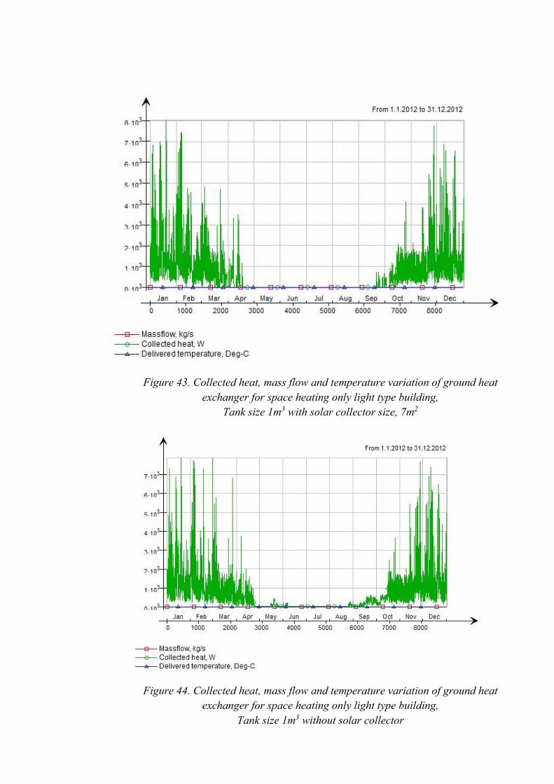
Figure 43. Collected heat, mass flow and temperature variation of ground heat
exchanger for space heating only light type building,
Tank size 1m3 with solar collector size, 7m2
Figure 44. Collected heat, mass flow and temperature variation of ground heat
exchanger for space heating only light type building,
Tank size 1m3 without solar collector

As it shows in the graph, tank connected to the solar collector gathers less heat from the
heat exchanger, because solar collector works to make the tank temperature higher, heat
exchanger connected to the heat pump generates less energy. This can check in the heat
pump electricity consumption when the solar collector is on or off state.
Figure 45 and 46 shows how the electricity consumption fluctuates by the solar collector
installation. This case also applies the light building with tank size of 1m3 and solar
collector size of 7m2. When the solar collector is used, heat pump spends less energy and
in the summer season, it becomes almost zero compared with heat pump model without
solar collector.
When it comes to the Coefficient of Performance (COP), the effect of solar thermal is
notable as figure 47 and figure 48 displays. It also demonstrates that in case of two storage
tanks, solar collector better adopts to the low temperature tank for space heating than high
temperature tank for domestic hot water usage. As it shows in one tank model, in the
stratified tank, COP of the heat pump becomes higher with the solar collector because
solar collector offers the heat transfer to the tank and occupies the lower temperature
portion of the tank; heat pump only works for the high temperature layer of the tank.

Figure 45. Heat pump electricity consumption
For space heating only light type building,
Tank size 1 m3 solar collector size, 7 m2
Figure 46. Heat pump electricity consumption
For space heating only light type building, tank size 1 m3 without solar collector

Figure 47. Coefficient of Performance (COP) variation of heat pump
For space heating only light type building, tank size 1 m3
Solar collector size,7 m2
Figure 48. Coefficient of Performance (COP) variation of heat pump
For space heating only light type building, tank size 1 m3 without solar collector

Solar collector effect can check more in the table 5 comparing with two energy utilization
results.
Table 6. Utilized energy from the system for space heating only model
In the light type building,
Tank size 1m3 with 7m2solar collector / without solar collector
Higher COP, more heat collected and less energy usage in the space heating with solar
collector model studies that control strategy in the low temperature tank is dependent on
the simulation result of solar collector operation and low temperature inner state in the
energy balance side. Space heating only models generate 132 samples in this case, result
shall adopt in control and optimization combining domestic hot water only tank model.
7.1.2 The result of high temperature tank control strategy
High temperature tank control follows domestic hot water only tank case. From the
standard IDA one tank model, it deletes the function of AHU and solar collector. It only
tags along the domestic hot water usage profile from occupants by the tank size;
temperature fluctuation inside of thermal tank decides in figure 49. Compared with
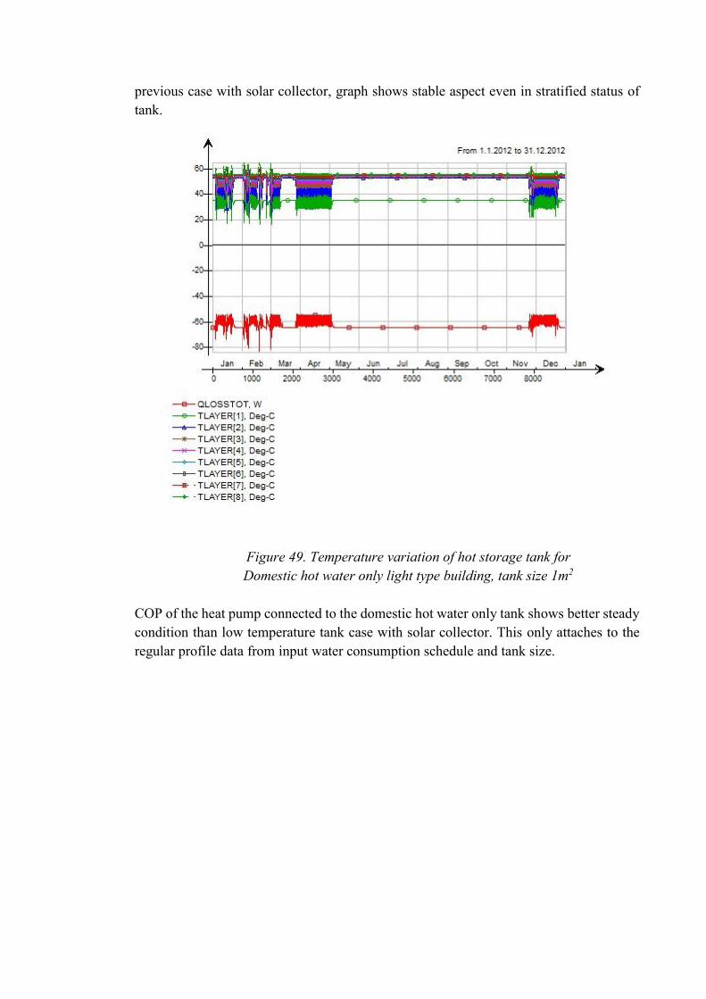
previous case with solar collector, graph shows stable aspect even in stratified status of
tank.
Figure 49. Temperature variation of hot storage tank for
Domestic hot water only light type building, tank size 1m2
COP of the heat pump connected to the domestic hot water only tank shows better steady
condition than low temperature tank case with solar collector. This only attaches to the
regular profile data from input water consumption schedule and tank size.
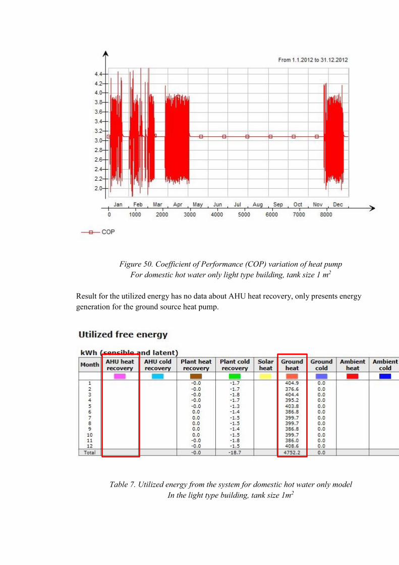
Figure 50. Coefficient of Performance (COP) variation of heat pump
For domestic hot water only light type building, tank size 1 m2
Result for the utilized energy has no data about AHU heat recovery, only presents energy
generation for the ground source heat pump.
Table 7. Utilized energy from the system for domestic hot water only model
In the light type building, tank size 1m2

For combining the result and producing optimization, 4 each domestic hot water only case
(0.5m3, 1m3, 1.5m3, 2m3) in the light weight, medium and massive passive type of
building is considered. 12 amounts of samples for three-insulation type of buildings can
generate.
7.1.3 The result of solar collector control strategy
Solar collector balances up the energy generation of the heat pump as it discussed
previous. Hence, solar collector and low temperature tank control demonstrates directly
how the heat collected from the solar collector works for compensating the energy
utilization of the heat pump. Figure 51 is the heat collected from the solar collector in the
light building type when the size of solar collector is 7m2. This result can compare with
low temperature tank collected heat and temperature variation discussed in previous
chapter.
Figure 51. Heat collected from the solar thermal for
Space heating only light type building,
Tank size 1 m3 with solar collector size, 7 m2
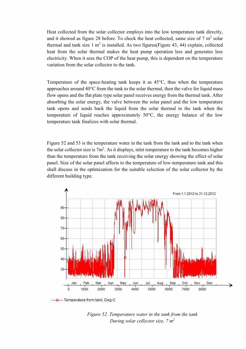
Heat collected from the solar collector employs into the low temperature tank directly,
and it showed as figure 28 before. To check the heat collected, same size of 7 m2 solar
thermal and tank size 1 m3 is installed. As two figures(Figure 43, 44) explain, collected
heat from the solar thermal makes the heat pump operation less and generates less
electricity. When it sees the COP of the heat pump, this is dependent on the temperature
variation from the solar collector to the tank.
Temperature of the space-heating tank keeps it as 45°C, thus when the temperature
approaches around 40°C from the tank to the solar thermal, then the valve for liquid mass
flow opens and the flat plate type solar panel receives energy from the thermal tank. After
absorbing the solar energy, the valve between the solar panel and the low temperature
tank opens and sends back the liquid from the solar thermal to the tank when the
temperature of liquid reaches approximately 50°C, the energy balance of the low
temperature tank finalizes with solar thermal.
Figure 52 and 53 is the temperature water in the tank from the tank and to the tank when
the solar collector size is 7m2. As it displays, inlet temperature to the tank becomes higher
than the temperature from the tank receiving the solar energy showing the effect of solar
panel. Size of the solar panel affects to the temperature of low-temperature tank and this
shall discuss in the optimization for the suitable selection of the solar collector by the
different building type.
Figure 52. Temperature water in the tank from the tank
During solar collector size, 7 m2

Figure 53. Temperature water in the tank to the tank
During solar collector size, 7 m2
7.2 Artificial neural network result
The results from the ANN shows error histogram and regression plot from figure 54 to
figure 65 as heat pump and solar collector energy generation by the type of building
envelope. Figure 54 and 55 is the error histogram and regression plot result for the neural
network in the lightweight building when the input vector decides as ground source heat
pump energy generated. In the figure 54, blue bars represent training data, the green bars
show validation data, and the red bars are testing data while the ideal zero error, so called
mean square error (MSE) is orange line. Histogram signifies the outliers, which are apart
from the major dataset, here shows as -95.57 in training when most cases fall between -
17.3 to 28.36. Checking the outlier data is good way to monitor the whole dataset if the
outlier data is valid point. If outliers are valid but unlike the rest of dataset as Figure 54,
network is extrapolating for these points. Another method is making more hidden neurons
and training trials repeatedly. In this plot, hidden neuron layer of 10 is used.
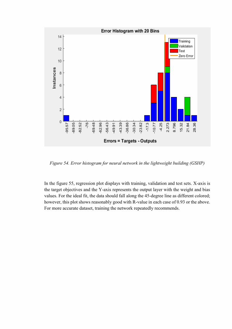
Figure 54. Error histogram for neural network in the lightweight building (GSHP)
In the figure 55, regression plot displays with training, validation and test sets. X-axis is
the target objectives and the Y-axis represents the output layer with the weight and bias
values. For the ideal fit, the data should fall along the 45-degree line as different colored;
however, this plot shows reasonably good with R-value in each case of 0.93 or the above.
For more accurate dataset, training the network repeatedly recommends.

Figure 55. Regression plot for neural network in the lightweight building (GSHP)
Solar collector heat generated vector also checks after making Artificial Neural Network.
Figure 56 and 57 is the error histogram and regression plot result for the neural network
in the lightweight building when the input vector decides as solar thermal collector energy
generated. As discussed previous, histogram outlines the boundary for the training,
validation and test dataset compared with the zero error line (Mean Square Error).
Regression plot also falls near to the ideal 45° slope from the ground line.
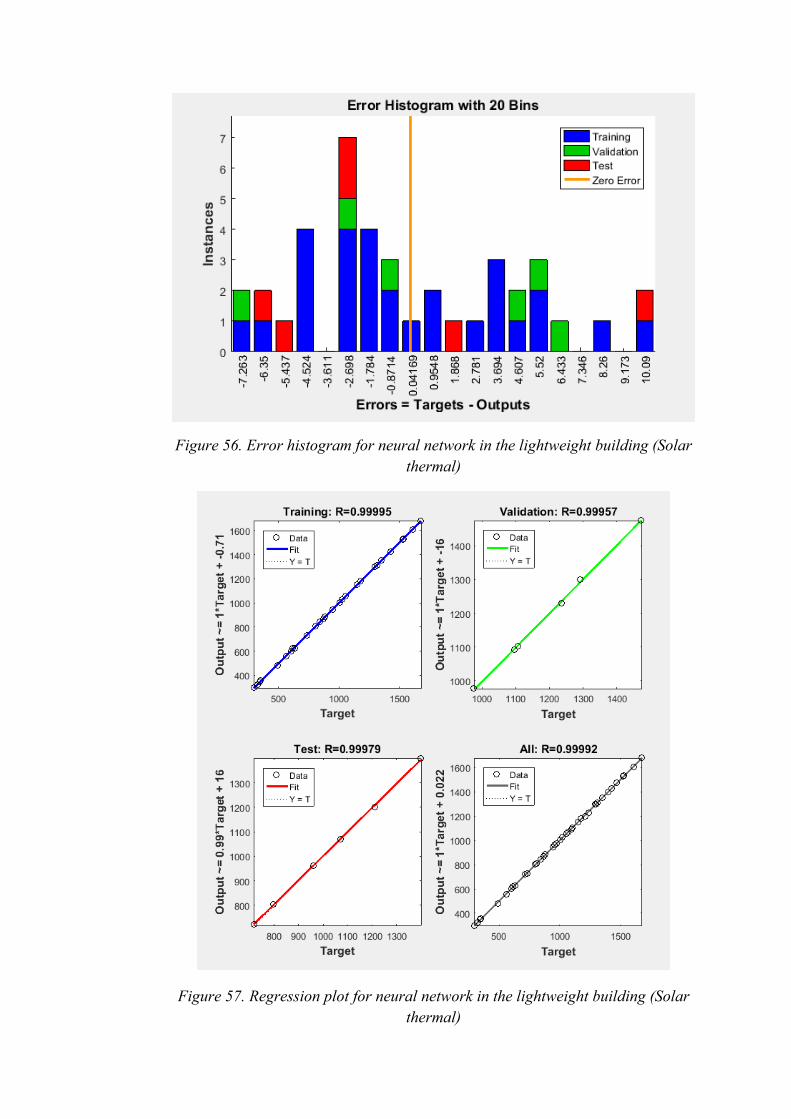
Figure 56. Error histogram for neural network in the lightweight building (Solar
thermal)
Figure 57. Regression plot for neural network in the lightweight building (Solar
thermal)
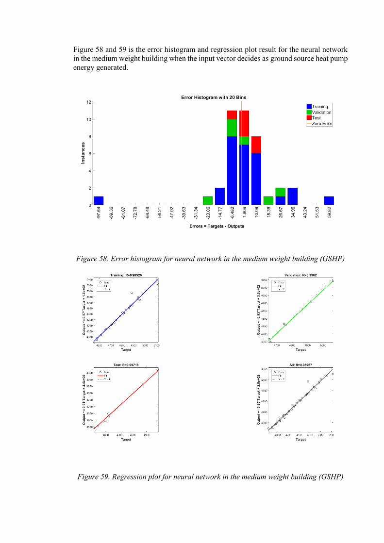
Figure 58 and 59 is the error histogram and regression plot result for the neural network
in the medium weight building when the input vector decides as ground source heat pump
energy generated.
Figure 58. Error histogram for neural network in the medium weight building (GSHP)
Figure 59. Regression plot for neural network in the medium weight building (GSHP)
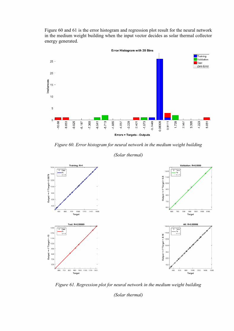
Figure 60 and 61 is the error histogram and regression plot result for the neural network
in the medium weight building when the input vector decides as solar thermal collector
energy generated.
Figure 60. Error histogram for neural network in the medium weight building
(Solar thermal)
Figure 61. Regression plot for neural network in the medium weight building
(Solar thermal)

Figure 62 and 63 is the error histogram and regression plot result for the neural network
in the massive weight building when the input vector decides as ground source heat pump
energy generated.
Figure 62. Error histogram for neural network in the massive weight building (GSHP)
Figure 63. Regression plot for neural network in the massive weight building (GSHP)
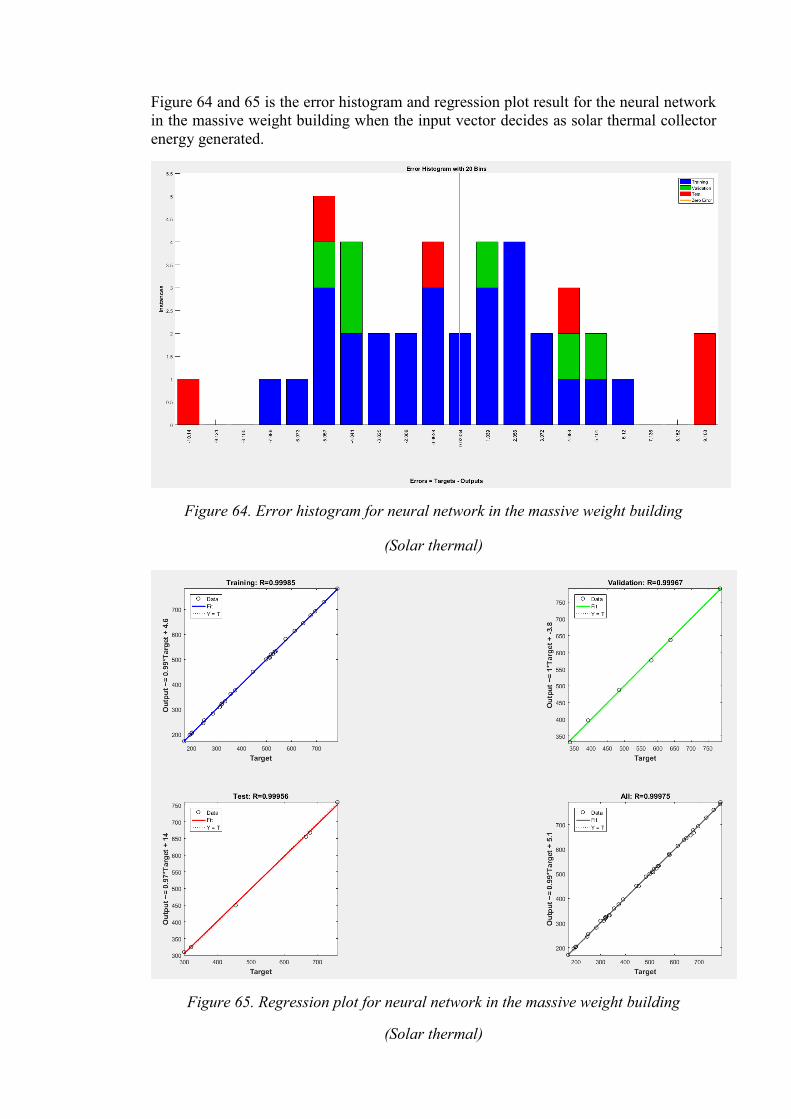
Figure 64 and 65 is the error histogram and regression plot result for the neural network
in the massive weight building when the input vector decides as solar thermal collector
energy generated.
Figure 64. Error histogram for neural network in the massive weight building
(Solar thermal)
Figure 65. Regression plot for neural network in the massive weight building
(Solar thermal)

The selected networks have the simpler structure and at the same time the best
performance. The simple structure is important, since the higher number of hidden layers
and neurons lead the model to over fitting. In over fitting because of high number of
hidden layer and corresponding neurons, the model estimates the reference data, which
are available in training set. Nevertheless, the model is not able to estimate those cases
out of training data set. To make the above graph of error histogram and regression plot
satisfying the reasonable result in the view of performance and avoiding overfitting,
histogram result is checked to make bars enter similar to the mean square error line, while
regression plot R value falls less behind 0.93 value. ANN result from the solar collector
input layer shows less error than when it comes to the input layer signifies as the heat
pump, general target output of solar collector energy generation is less than the heat pump
electricity consumption. Compared with the light and medium type of building, massive
building shows less error because building shape is passive type good for insulation and
better for storing the energy thus less energy generation is required from the target input
layer fulfilling the zero-energy building case.
7.3 Multi Objective optimization result
7.3.1 Cost of energy components
The price for components shows as values in table 8. This information is a part of wide
price data set gathered by HVAC technology research group. For the electricity, the price
considers as 11 (c/kWh) which includes those factors in Table 8.
Finish VAT Electricity tax
(c/kWh)
Company
margin
(c/kWh)
Distribution
cost
(c/kWh)
Feed-in tariff
(c/kWh)
24% 2.79372 0.3 3.98 8.35
Table 8. Electricity price based on information of 2012
For thermal solar panel the unit price is 609 (€/m2). This price is average of available
information from HP4NZEB in Aalto price data. The information in HP4NZEB estimates
based on real projects. For the tank, the price extracts according to information of
AKVATERM Company for thermal tank type series as Table 9 demonstrates.

Height
(m)
Diameter
(m)
Volume
(m3)
Price
(€)
Unit price
(€/m3)
2.050 0.650 0.68 1819.00 2675.36
2.050 0.800 1.03 2199.00 2135.12
2.050 0.950 1.45 2305.00 1587.09
2.100 1.050 1.82 2579.00 1419.00
2.150 1.250 2.64 3285.00 1245.68
2.250 1.400 3.46 3649.00 1054.06
2.250 1.500 3.97 3339.00 840.20
2.300 1.600 4.62 3539.00 765.67
2.350 1.800 5.98 4799.00 802.91
Table 9. Price of the hot water storage tank
In the end the LCC can present as
𝐿𝐶𝐶20 = 𝐼𝑛𝑣 + 𝑀 − 𝐸𝑛𝑒 (35)
where
𝐼𝑛𝑣 Investment cost for the summation of thermal solar collector
With tank price
M Maintenance Cost (when investment cost is 3%)
Ene Energy profit{(𝐴𝑛𝑛𝑢𝑎𝑙 𝑠𝑜𝑙𝑎𝑟 ℎ𝑒𝑎𝑡 𝑐𝑜𝑙𝑙𝑒𝑐𝑡𝑒𝑑) ∗ (0.011)}
7.3.2 Optimal selection of two tanks and solar collector
The results of thermal solar system for three types of building presents in previous
sections with control part. By the control equation (30), connected case considers and it
compares with the non-connected case. Connected case is, when two-tank model assumes
as the one tank system and get the balance equation between them. Non-connected case
is simple the sum of heat demand for the domestic hot water only tank and space heating
only tank model without solar collector. The multi objective optimization carries out for
minimizing the energy consumption of ground source heat pump and life cycle cost in
light, medium and massive type of building.

The results for non-connected and connected cases shows in Figures 66 and 67 with
Pareto Front.
Figure 66. Pareto front for different types of building (Non-connected case)

Figure 67. Pareto front for different types of building (Connected case)
The results show that the electricity consumption and cost of the system for massive type
building is significantly lower in compared with two other building types. This trend is
same in both states of connected and non-connected cases. Furthermore, connected case
demonstrates the wide range of selection for the suitable solar collector and tank. It also
shows higher energy efficiency compared with non-connected case. This shall discuss as
effect of solar collector.
For studying the effect of economic parameters on optimal results, the interest rate
changes from 3% to 9%. The effect of the varying the interest rate is studied on state of
connecting two storage tanks for massive and lightweight buildings to check the
significant differences. The results shows in figure 68 and 69.

Figure 68. Life cycle cost result considering economic parameter in Light type building
Figure 69. Life cycle cost result considering economic parameter in
Massive type building
The results demonstrate that by increasing the interest rate, the life cycle cost reduces and
system efficiency goes higher (less electricity usage). In case of massive building, the
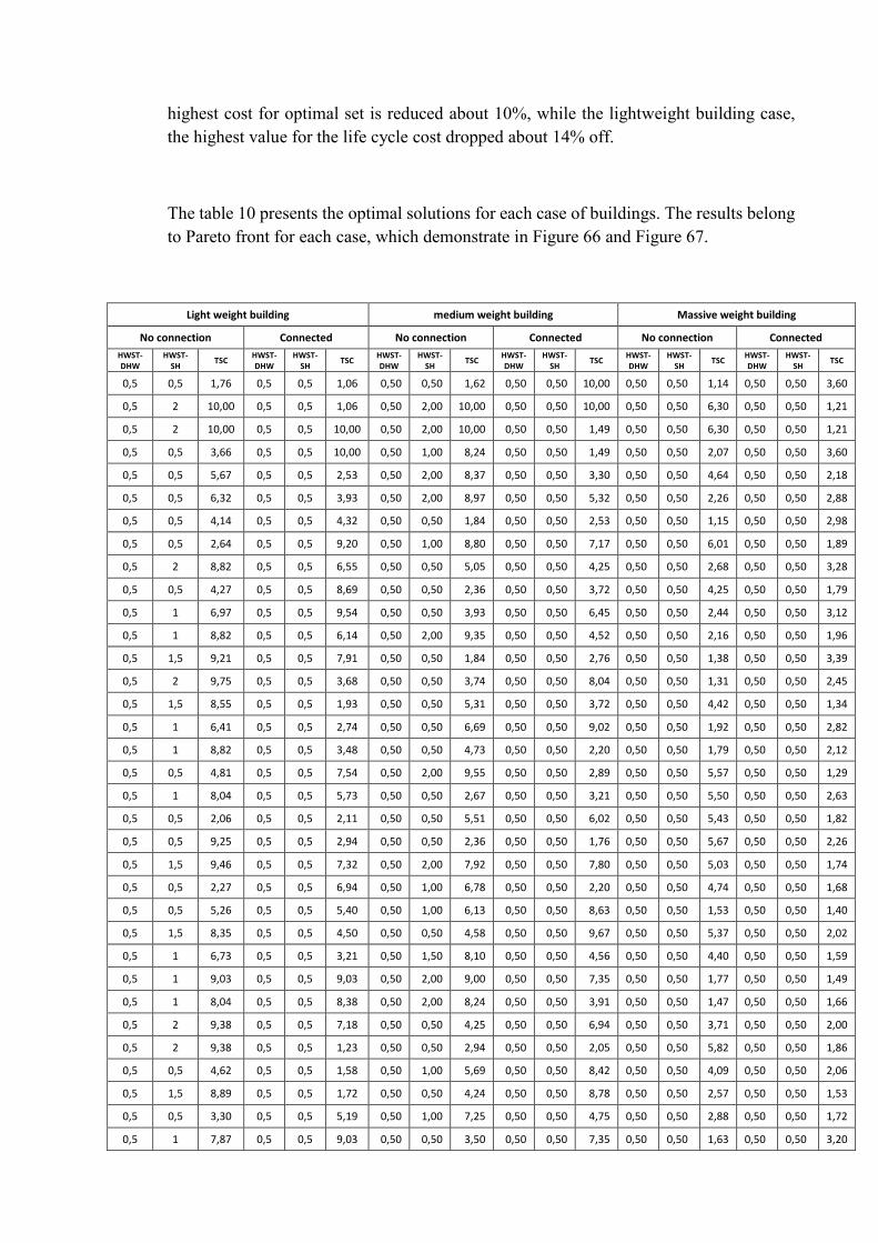
highest cost for optimal set is reduced about 10%, while the lightweight building case,
the highest value for the life cycle cost dropped about 14% off.
The table 10 presents the optimal solutions for each case of buildings. The results belong
to Pareto front for each case, which demonstrate in Figure 66 and Figure 67.
Light weight building medium weight building Massive weight building
No connection Connected No connection Connected No connection Connected
HWST-DHW
HWST-SH
TSC HWST-DHW
HWST-SH
TSC HWST-DHW
HWST-SH
TSC HWST-DHW
HWST-SH
TSC HWST-DHW
HWST-SH
TSC HWST-DHW
HWST-SH
TSC
0,5 0,5 1,76 0,5 0,5 1,06 0,50 0,50 1,62 0,50 0,50 10,00 0,50 0,50 1,14 0,50 0,50 3,60
0,5 2 10,00 0,5 0,5 1,06 0,50 2,00 10,00 0,50 0,50 10,00 0,50 0,50 6,30 0,50 0,50 1,21
0,5 2 10,00 0,5 0,5 10,00 0,50 2,00 10,00 0,50 0,50 1,49 0,50 0,50 6,30 0,50 0,50 1,21
0,5 0,5 3,66 0,5 0,5 10,00 0,50 1,00 8,24 0,50 0,50 1,49 0,50 0,50 2,07 0,50 0,50 3,60
0,5 0,5 5,67 0,5 0,5 2,53 0,50 2,00 8,37 0,50 0,50 3,30 0,50 0,50 4,64 0,50 0,50 2,18
0,5 0,5 6,32 0,5 0,5 3,93 0,50 2,00 8,97 0,50 0,50 5,32 0,50 0,50 2,26 0,50 0,50 2,88
0,5 0,5 4,14 0,5 0,5 4,32 0,50 0,50 1,84 0,50 0,50 2,53 0,50 0,50 1,15 0,50 0,50 2,98
0,5 0,5 2,64 0,5 0,5 9,20 0,50 1,00 8,80 0,50 0,50 7,17 0,50 0,50 6,01 0,50 0,50 1,89
0,5 2 8,82 0,5 0,5 6,55 0,50 0,50 5,05 0,50 0,50 4,25 0,50 0,50 2,68 0,50 0,50 3,28
0,5 0,5 4,27 0,5 0,5 8,69 0,50 0,50 2,36 0,50 0,50 3,72 0,50 0,50 4,25 0,50 0,50 1,79
0,5 1 6,97 0,5 0,5 9,54 0,50 0,50 3,93 0,50 0,50 6,45 0,50 0,50 2,44 0,50 0,50 3,12
0,5 1 8,82 0,5 0,5 6,14 0,50 2,00 9,35 0,50 0,50 4,52 0,50 0,50 2,16 0,50 0,50 1,96
0,5 1,5 9,21 0,5 0,5 7,91 0,50 0,50 1,84 0,50 0,50 2,76 0,50 0,50 1,38 0,50 0,50 3,39
0,5 2 9,75 0,5 0,5 3,68 0,50 0,50 3,74 0,50 0,50 8,04 0,50 0,50 1,31 0,50 0,50 2,45
0,5 1,5 8,55 0,5 0,5 1,93 0,50 0,50 5,31 0,50 0,50 3,72 0,50 0,50 4,42 0,50 0,50 1,34
0,5 1 6,41 0,5 0,5 2,74 0,50 0,50 6,69 0,50 0,50 9,02 0,50 0,50 1,92 0,50 0,50 2,82
0,5 1 8,82 0,5 0,5 3,48 0,50 0,50 4,73 0,50 0,50 2,20 0,50 0,50 1,79 0,50 0,50 2,12
0,5 0,5 4,81 0,5 0,5 7,54 0,50 2,00 9,55 0,50 0,50 2,89 0,50 0,50 5,57 0,50 0,50 1,29
0,5 1 8,04 0,5 0,5 5,73 0,50 0,50 2,67 0,50 0,50 3,21 0,50 0,50 5,50 0,50 0,50 2,63
0,5 0,5 2,06 0,5 0,5 2,11 0,50 0,50 5,51 0,50 0,50 6,02 0,50 0,50 5,43 0,50 0,50 1,82
0,5 0,5 9,25 0,5 0,5 2,94 0,50 0,50 2,36 0,50 0,50 1,76 0,50 0,50 5,67 0,50 0,50 2,26
0,5 1,5 9,46 0,5 0,5 7,32 0,50 2,00 7,92 0,50 0,50 7,80 0,50 0,50 5,03 0,50 0,50 1,74
0,5 0,5 2,27 0,5 0,5 6,94 0,50 1,00 6,78 0,50 0,50 2,20 0,50 0,50 4,74 0,50 0,50 1,68
0,5 0,5 5,26 0,5 0,5 5,40 0,50 1,00 6,13 0,50 0,50 8,63 0,50 0,50 1,53 0,50 0,50 1,40
0,5 1,5 8,35 0,5 0,5 4,50 0,50 0,50 4,58 0,50 0,50 9,67 0,50 0,50 5,37 0,50 0,50 2,02
0,5 1 6,73 0,5 0,5 3,21 0,50 1,50 8,10 0,50 0,50 4,56 0,50 0,50 4,40 0,50 0,50 1,59
0,5 1 9,03 0,5 0,5 9,03 0,50 2,00 9,00 0,50 0,50 7,35 0,50 0,50 1,77 0,50 0,50 1,49
0,5 1 8,04 0,5 0,5 8,38 0,50 2,00 8,24 0,50 0,50 3,91 0,50 0,50 1,47 0,50 0,50 1,66
0,5 2 9,38 0,5 0,5 7,18 0,50 0,50 4,25 0,50 0,50 6,94 0,50 0,50 3,71 0,50 0,50 2,00
0,5 2 9,38 0,5 0,5 1,23 0,50 0,50 2,94 0,50 0,50 2,05 0,50 0,50 5,82 0,50 0,50 1,86
0,5 0,5 4,62 0,5 0,5 1,58 0,50 1,00 5,69 0,50 0,50 8,42 0,50 0,50 4,09 0,50 0,50 2,06
0,5 1,5 8,89 0,5 0,5 1,72 0,50 0,50 4,24 0,50 0,50 8,78 0,50 0,50 2,57 0,50 0,50 1,53
0,5 0,5 3,30 0,5 0,5 5,19 0,50 1,00 7,25 0,50 0,50 4,75 0,50 0,50 2,88 0,50 0,50 1,72
0,5 1 7,87 0,5 0,5 9,03 0,50 0,50 3,50 0,50 0,50 7,35 0,50 0,50 1,63 0,50 0,50 3,20
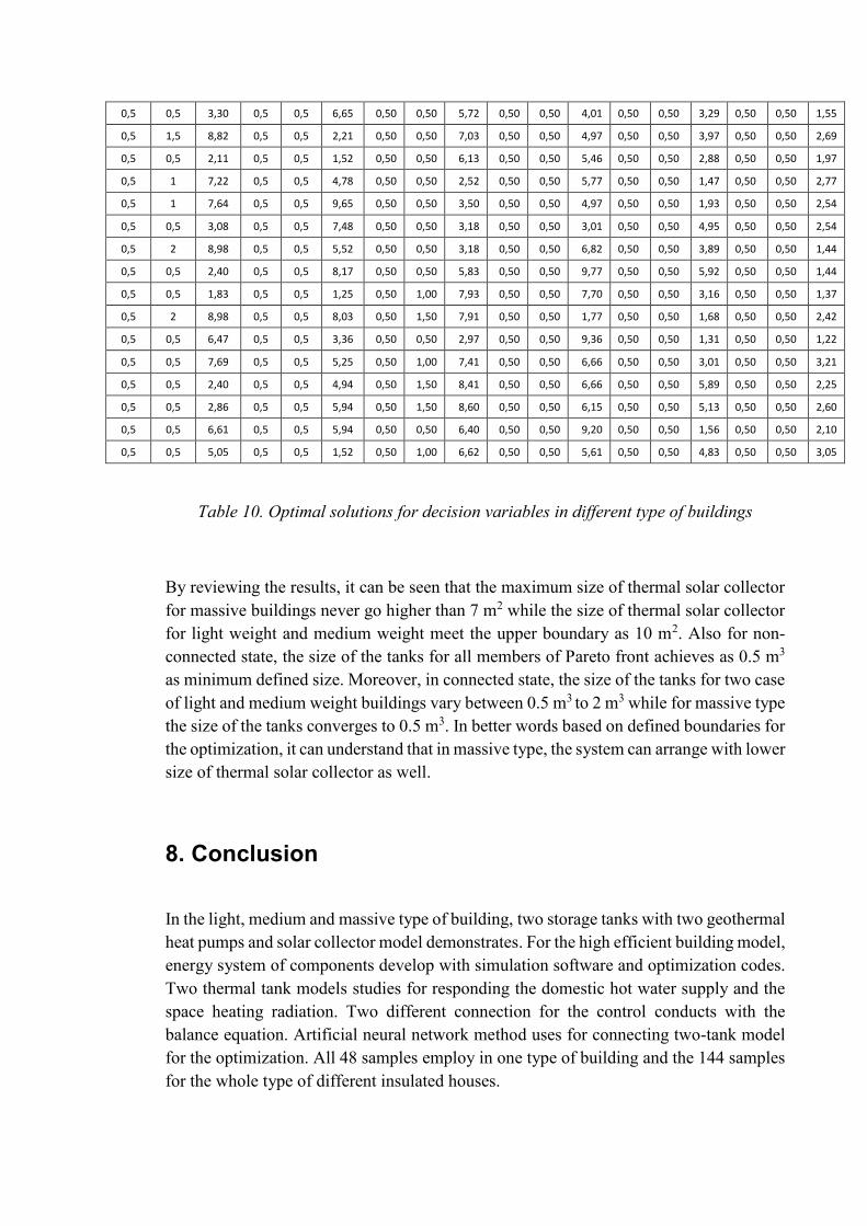
0,5 0,5 3,30 0,5 0,5 6,65 0,50 0,50 5,72 0,50 0,50 4,01 0,50 0,50 3,29 0,50 0,50 1,55
0,5 1,5 8,82 0,5 0,5 2,21 0,50 0,50 7,03 0,50 0,50 4,97 0,50 0,50 3,97 0,50 0,50 2,69
0,5 0,5 2,11 0,5 0,5 1,52 0,50 0,50 6,13 0,50 0,50 5,46 0,50 0,50 2,88 0,50 0,50 1,97
0,5 1 7,22 0,5 0,5 4,78 0,50 0,50 2,52 0,50 0,50 5,77 0,50 0,50 1,47 0,50 0,50 2,77
0,5 1 7,64 0,5 0,5 9,65 0,50 0,50 3,50 0,50 0,50 4,97 0,50 0,50 1,93 0,50 0,50 2,54
0,5 0,5 3,08 0,5 0,5 7,48 0,50 0,50 3,18 0,50 0,50 3,01 0,50 0,50 4,95 0,50 0,50 2,54
0,5 2 8,98 0,5 0,5 5,52 0,50 0,50 3,18 0,50 0,50 6,82 0,50 0,50 3,89 0,50 0,50 1,44
0,5 0,5 2,40 0,5 0,5 8,17 0,50 0,50 5,83 0,50 0,50 9,77 0,50 0,50 5,92 0,50 0,50 1,44
0,5 0,5 1,83 0,5 0,5 1,25 0,50 1,00 7,93 0,50 0,50 7,70 0,50 0,50 3,16 0,50 0,50 1,37
0,5 2 8,98 0,5 0,5 8,03 0,50 1,50 7,91 0,50 0,50 1,77 0,50 0,50 1,68 0,50 0,50 2,42
0,5 0,5 6,47 0,5 0,5 3,36 0,50 0,50 2,97 0,50 0,50 9,36 0,50 0,50 1,31 0,50 0,50 1,22
0,5 0,5 7,69 0,5 0,5 5,25 0,50 1,00 7,41 0,50 0,50 6,66 0,50 0,50 3,01 0,50 0,50 3,21
0,5 0,5 2,40 0,5 0,5 4,94 0,50 1,50 8,41 0,50 0,50 6,66 0,50 0,50 5,89 0,50 0,50 2,25
0,5 0,5 2,86 0,5 0,5 5,94 0,50 1,50 8,60 0,50 0,50 6,15 0,50 0,50 5,13 0,50 0,50 2,60
0,5 0,5 6,61 0,5 0,5 5,94 0,50 0,50 6,40 0,50 0,50 9,20 0,50 0,50 1,56 0,50 0,50 2,10
0,5 0,5 5,05 0,5 0,5 1,52 0,50 1,00 6,62 0,50 0,50 5,61 0,50 0,50 4,83 0,50 0,50 3,05
Table 10. Optimal solutions for decision variables in different type of buildings
By reviewing the results, it can be seen that the maximum size of thermal solar collector
for massive buildings never go higher than 7 m2 while the size of thermal solar collector
for light weight and medium weight meet the upper boundary as 10 m2. Also for non-
connected state, the size of the tanks for all members of Pareto front achieves as 0.5 m3
as minimum defined size. Moreover, in connected state, the size of the tanks for two case
of light and medium weight buildings vary between 0.5 m3 to 2 m3 while for massive type
the size of the tanks converges to 0.5 m3. In better words based on defined boundaries for
the optimization, it can understand that in massive type, the system can arrange with lower
size of thermal solar collector as well.
8. Conclusion
In the light, medium and massive type of building, two storage tanks with two geothermal
heat pumps and solar collector model demonstrates. For the high efficient building model,
energy system of components develop with simulation software and optimization codes.
Two thermal tank models studies for responding the domestic hot water supply and the
space heating radiation. Two different connection for the control conducts with the
balance equation. Artificial neural network method uses for connecting two-tank model
for the optimization. All 48 samples employ in one type of building and the 144 samples
for the whole type of different insulated houses.
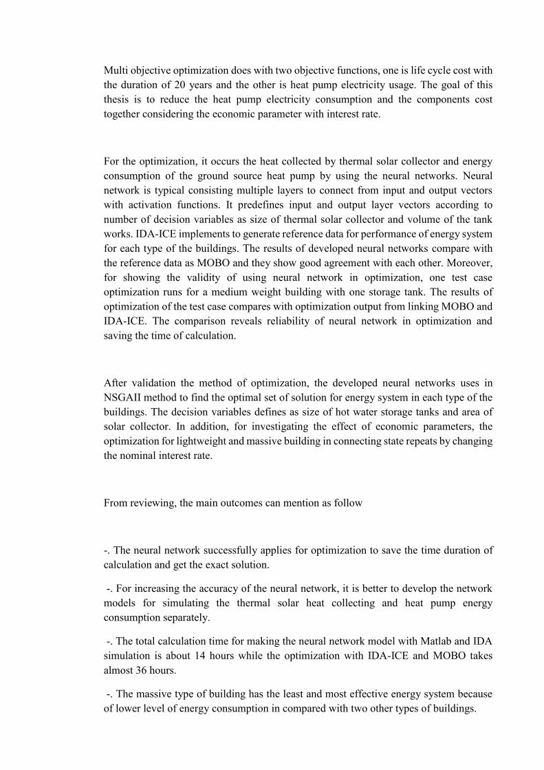
Multi objective optimization does with two objective functions, one is life cycle cost with
the duration of 20 years and the other is heat pump electricity usage. The goal of this
thesis is to reduce the heat pump electricity consumption and the components cost
together considering the economic parameter with interest rate.
For the optimization, it occurs the heat collected by thermal solar collector and energy
consumption of the ground source heat pump by using the neural networks. Neural
network is typical consisting multiple layers to connect from input and output vectors
with activation functions. It predefines input and output layer vectors according to
number of decision variables as size of thermal solar collector and volume of the tank
works. IDA-ICE implements to generate reference data for performance of energy system
for each type of the buildings. The results of developed neural networks compare with
the reference data as MOBO and they show good agreement with each other. Moreover,
for showing the validity of using neural network in optimization, one test case
optimization runs for a medium weight building with one storage tank. The results of
optimization of the test case compares with optimization output from linking MOBO and
IDA-ICE. The comparison reveals reliability of neural network in optimization and
saving the time of calculation.
After validation the method of optimization, the developed neural networks uses in
NSGAII method to find the optimal set of solution for energy system in each type of the
buildings. The decision variables defines as size of hot water storage tanks and area of
solar collector. In addition, for investigating the effect of economic parameters, the
optimization for lightweight and massive building in connecting state repeats by changing
the nominal interest rate.
From reviewing, the main outcomes can mention as follow
-. The neural network successfully applies for optimization to save the time duration of
calculation and get the exact solution.
-. For increasing the accuracy of the neural network, it is better to develop the network
models for simulating the thermal solar heat collecting and heat pump energy
consumption separately.
-. The total calculation time for making the neural network model with Matlab and IDA
simulation is about 14 hours while the optimization with IDA-ICE and MOBO takes
almost 36 hours.
-. The massive type of building has the least and most effective energy system because
of lower level of energy consumption in compared with two other types of buildings.

-. In non-connected state, the size of tanks in all types of buildings converged to
minimum defined size as 0.5 m3. The size of solar collector in non -connected state is
higher for lightweight and medium weight buildings.
-. In connected state the efficiency of energy system and life cycle cost for all buildings
types are improved. In connected state, the optimal size of warm tank is bigger than hot
tank. It is because of using of warm tanks for two targets as responding to space heating
demand and pre heating the hot tank.
-. Electricity price is fixed and only component costs considers to make the optimal
selection.
-. Different interest rates considering various economic parameters for the LCC
calculation demonstrates that by increasing the nominal interest rate, the feasibility of
optimal solution increases.
-. More than one tank model can easily apply to the IDA simulation using balance
equation.
References
COMMUNICATION FROM THE COMMISSION TO THE EUROPEAN
PARLIAMENT, THE COUNCIL, THE EUROPEAN ECONOMIC AND SOCIAL
COMMITTEE AND THE COMMITTEE OF THE REGIONS A policy framework for
climate and energy in the period from 2020 to 2030.
European Commission - Energy Roadmap 2050, Luxembourg: Publications Office of
the European Union. Available at:
https://ec.europa.eu/energy/sites/ener/files/documents/2012_energy_roadmap_2050_en
_0.pdf
United Nations Environment Program, environment for development. Available at:
http://www.unep.org/sbci/AboutSBCI/Background.asp
US energy Information administration. Available at : http://www.eia.gov/
EU ETS Handbook. Available at :
http://ec.europa.eu/clima/publications/docs/ets_handbook_en.pdf
Strategy for energy renovation of buildings: The route to energy efficient buildings in
tomorrow’s Denmark : available at
https://ec.europa.eu/energy/sites/ener/files/documents/2014_article4_en_denmark.pdf
David Shearer, Dr Brian Anderson, Building Research Establishment, International
comparison of energy standards in building regulations for non-domestic buildings:
Denmark, Finland, Norway, Scotland, and Sweden by the Scotish government. Avaialbe
at : http://www.gov.scot/resource/doc/217736/0113670.pdf
K.Imessad, N.Ait Messaoudene, M.Belhamel. Performance of the BARRA-Costantini
passive heating system under Algerian climate conditions
Bioenergy in Finland, Energy for sustainable development. Available at:
www.unep.org/GC/GCSS-IX/Documents/FINLAND-bioenergy.pdf
Advantages of heating with wood. From tulikivi company. Avaialbe at :
http://www.tulikivi.com/en/tulikivi/Advantages_of_heating_with_wood
Zero Energy House, Järvenpää in 2010 by GBC. Available at : http://figbc.fi/en/building-
sector/zero-energy-house-jarvenpaa/
Finnish Energy, Combines Heat and Power Generation. Available at :
http://energia.fi/en/energy-and-environment/district-heat-and-district-cooling/combined-
heat-and-power-generation
Building retro by Charles Lockwood in 2009. Available at :
https://www.esbnyc.com/sites/default/files/uli_building_retro_fits.pdf
Buildings Performance Institute Europe (BPIE), ‘Gaining knowledge of the EU building
stock’ Oliver Rapf, BPIE 30 March 2014, Beijing, EU China Trade Project II.

Suresh B. Sadineni, Srikanth Madala, Robert F. Boehm. Passive building energy savings:
A review of building envelope components, Renewable and Sustainable Energy Reviews
15 (2011) 3617–3631
Illikainen Kimmo, Sirviö Anu ’Sustainable Buildings for the High North. Existing
buildings – technologies and challenges for residential and commercial use’ 7.10.2015
Avaialbe at : http://www.oamk.fi/epooki/2015/high-north-project-existing-buildings/
Abhishek Subba, ‘Hygrothermal Behavior of Finnish Building Exterior Walls’ Degree
Programme in Construction Engineering. HAMK University of applied science. Avaialbe
at : http://www.theseus.fi/bitstream/handle/10024/87107/final+-
+Hygrothermal+behavior+of+finnish+building+exterior+walls-
Abhishek+SubbaV2.pdf;jsessionid=435D80F21F3D71EB6621E7C83934978A?sequen
ce=1
FIN3 Building code D3: Energy efficiency of new buildings 1st April 2016, Available at:
http://www.measures-odyssee-mure.eu/public/mure_pdf/household/FIN3.PDF
National Building code of Finland. Avaiable at : http://www.ym.fi/en-
us/Land_use_and_building/Legislation_and_instructions/The_National_Building_Code
_of_Finland
Decree of Ministry of the Environment on thermal insulation in a building, issued in
Helsinki on 30 October 2002. Available at :
https://www.edilex.fi/data/rakentamismaaraykset/c3e_2003.pdf
FIN3 Building code D3: Energy efficiency of new buildings. Available at :
http://www.measures-odyssee-mure.eu/public/mure_pdf/household/FIN3.PDF
Hiroki Matsumoto, Yoshio Iwai, Hiroshi Ishiguro. ‘Estimation of Thermal Comfort by
Measuring Clo Value without Contact’ MVA2011 IAPR Conference on Machine Vision
Applications, June 13-15, 2011, Nara, JAPAN. Graduate School of Engineering Science,
Osaka University.
Contact to : [email protected]
Hyesim Han a, Jinsook Lee b, Jonghun Kim a, Cheolyong Jang a, Hakgeun Jeong a
‘Thermal Comfort Control Based on a Simplified Predicted Mean Vote index’ Volume
61, 2014, Pages 970-974. International Conference on Applied Energy, ICAE2014
Pouya Samania, Vítor Lealb, Adélio Mendesc, Nuno Correiad ‘Comparison of passive
cooling techniques in improving thermal comfort of occupants of a pre-fabricated
building’ Energy and Buildings. Volume 120, 15 May 2016, Pages 30–44
Esco Tähti, Howard Goodfellow ‘Industrial Ventilation Design Guidebook’ Department
of Chemical Engineering and Applied Chemistry University of Toronto.
Marko Hannanonen. ‘A Field theory of house prices: An Empirical Study of the Helsinki
submarket
’ ISBN 978-952-6613-36-9
‘World Air Conditioner Demand by Region’ The Japan Refrigeration and Air
Conditioning Industry Association, April 2016. Available at : http://www.jraia.or.jp

M. Ciampi, F. Leccese, G. Tuoni Ventilated facades energy performance in summer
cooling of buildings Solar Energy, 75 (6) (2003), pp. 491–502
Syed Ihtsham ul Haq Gilani ‘Thermal Comfort Analysis of PMV Model Prediction in Air
Conditioned and Naturally Ventilated Buildings’ Energy Procedia Volume 75, August
2015, Pages 1373-1379 Clean, Efficient and Affordable Energy for a Sustainable Future:
The 7th International Conference on Applied Energy (ICAE2015)
The Finnish Heat Pump Association (SULPU) available at :
http://www.sulpu.fi/documents/184029/189661/Heat%20Pump%20basics.pdf
"Choosing and Installing Geothermal Heat Pumps". Energy.gov. Retrieved 30 September
2014.
Lowe, Robert (2011). "Combined heat and power considered as a virtual steam cycle heat
pump". Energy Policy. 39 (9): 5528–5534. doi:10.1016/j.enpol.2011.05.007. ISSN 0301-
4215.
Mitsubishi electric heat pump CAHV-P500YA-HPB. Available at :
https://heating.mitsubishielectric.co.uk/KnowledgeBase/Public/CAHV%20PI%20Sheet.
Laitinen, A., Tuominen, P., Holopainen, R., Tuomaala, P., Jokisalo, J., Eskola, L. and
Sirén, K. 2013. Renewable energy production of Finnish heat pumps. VTT. Available
at :
http://www.vtt.fi/inf/pdf/technology/2014/T164.pdf
Vijay Dwivedi (Reg. No. 200858672). ‘Thermal Modelling and Control of Domestic
Hot water Tank’ from the department of Mechanical Engineering in the University of
Strathclyde, Master of Science in Energy Systems and the Environment
Fabio Struckmann.’Analysis of a Flat plate Solar Collector’ Dept of Energy Science,
Faculty of Engineering in Lund University. 2008 MVK 160 Heat and Mass Transport.
May 08.2008. Lund Sweden.
Duffie J. A., Beckman W. A., 2006, Solar Engineering of Thermal Processes, John Wiley
and Sons, USA.
Alimohammadisagvand B, Alam S, Ali M, Degefa M, Jokisalo J, Siren K. Influence of
energy demand response actions on thermal comfort and energy cost in electrically heated
residential houses. Indoor Built Environ 2015.
http://dx.doi.org/10.1177/1420326X15608514.
Jukka Yrjölä * and Eetu Laaksonen; Domestic Hot Water Production with Ground Source
Heat Pump in Apartment buildings, p5. Energies 2015, 8, 8447-8466, ISSN 1996-1073,
Avaialbe at : www.mdpi.com/journal/energies
Henry Nasution, Azhar Abdul Aziz, Zulkarnain abdul Latiff. PI control Application for
building Air Conditioning System. Jurnal Teknologi 25 March 2015. Contact at :
HP4NZEB company. Available at : http://gnf.fi/fi/gnf/hp4nzeb-lampopumppukonseptit-
lahes-nollaenergiarakentamisessa/

AKVATERM company. Available at : http://www.akvaterm.fi/fin/Akvaterm.1.html
Matti Palonen, Mohmed Hamdy and Ala Hasan; proceedings of BS2013: 13th
Conference of international Building Performance Simulation Association, Chambery
France August 26-28 ‘MOBO A NEW SOFTWARE FOR MULTI-OBJECTIVE
BUILDING PERFORMANCE OPTIMIZATION’ Aalto University, VTT Technical
Research Centre of Finland, Espoo, Finland

Appendixes
Appendix 1. Detailed descriptions of the structure materials and characteristic features
Appendix 2. Technical specifications of the ground source heat pump systems used in
simulations
Appendix 3. Technical specifications of the solar thermal system used in the simulations.
Appendix 4. Technical descriptions of the energy system model in the IDA-ICE ESBO
plant.
Appendix 5. Life Cycle Cost analysis used in the optimization result.

Appendix 1. Detailed descriptions of the structure
materials and characteristic features
Light Weight Building
External wall (LW2010)
Structure
D,
m
λ,
W/mK
ρ,
kg/m³
cp,
J/kgK
R,
m²K/W
1 Gypsum (s) 0.013 0.22 970 1090 0.059
2 Frame cc600 0.247 0.044 56 1720 5.614
3 Wind Shield Board (s) 0.009 0.22 970 1090 0.041
Total U-value 0.17 W/m²K
Internal wall (LW)
Structure
D,
m
λ,
W/mK
ρ,
kg/m³
cp,
J/kgK
R,
m²K/W
1 Gypsum (s) 0.013 0.22 970 1090 0.059
2 Frame cc600 0.05 0.044 56 1720 1.137
3 Gypsum (s) 0.013 0.22 970 1090 0.059
Total U-value 0.702 W/m²K
Internal Floors (LW)
Structure
D,
m
λ,
W/mK
ρ,
kg/m³
cp,
J/kgK
R,
m²K/W
1 Parquet (s) 0.015 0.14 460 2300 0.107
2 Particle board (s) 0.022 0.13 1000 1300 0.169
3 Frame cc600 0.1 0.044 56 1720 2.273
4 Gypsum (s) 0.013 0.22 970 1090 0.059
Total U-value 0.3599 W/m²K

Roof (LW2010)
Structure
D,
m
λ,
W/mK
ρ,
kg/m³
cp,
J/kgK
R,
m²K/W
1 Mineral Wool 0.264 0.035 20 750 7.543
2 Frame cc600 0.15 0.044 56 1720 3.409
3 Gypsum (s) 0.013 0.22 970 1090 0.059
Total U-value 0.08944 W/m²K
External Floor (LW2010)
Structure
D,
m
λ,
W/mK
ρ,
kg/m³
cp,
J/kgK
R,
m²K/W
1 Parquet 0.014 0.14 460 2300 0.1
2 Frame cc600 0.475 0.044 56 1720 10.795
3 Wind shield board (s) 0.009 0.22 970 1090 0.041
Total U-value 0.09004 W/m²K

Medium Weight Building
External wall (M2010)
Structure
D,
m
λ,
W/mK
ρ,
kg/m³
cp,
J/kgK
R,
m²K/W
1 Lightweight concrete (s) 0.13 0.24 650 1000 0.542
2 Polyurethane thermal 0.24 0.05 70 1500 4.8
3 Lightweight concrete (s) 0.09 0.24 650 1000 0.375
Total U-value 0.1699 W/m²K
Internal wall (M)
Structure
D,
m
λ,
W/mK
ρ,
kg/m³
cp,
J/kgK
R,
m²K/W
1 Lightweight concrete (s) 0.1 0.24 650 1000 0.417
Total U-value 1.705 W/m²K
Internal Floors (M)
Structure
D,
m
λ,
W/mK
ρ,
kg/m³
cp,
J/kgK
R,
m²K/W
1 Parquet (s) 0.015 0.14 460 2300 0.107
2 Lightweight concrete (s) 0.015 0.135 500 100 0.111
3 Concrete (s) 0.1 1.7 2300 880 0.059
4 Filler (s) 0.005 0.9 1700 1000 0.0056
Total U-value 2.209 W/m²K
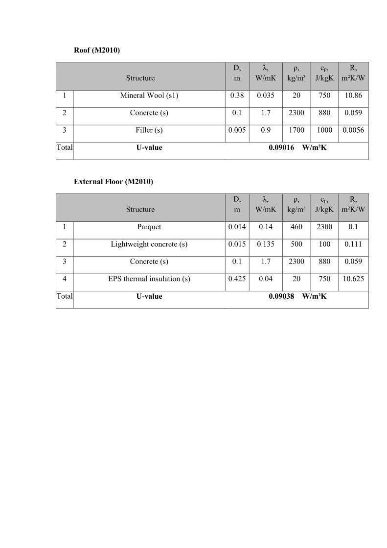
Roof (M2010)
Structure
D,
m
λ,
W/mK
ρ,
kg/m³
cp,
J/kgK
R,
m²K/W
1 Mineral Wool (s1) 0.38 0.035 20 750 10.86
2 Concrete (s) 0.1 1.7 2300 880 0.059
3 Filler (s) 0.005 0.9 1700 1000 0.0056
Total U-value 0.09016 W/m²K
External Floor (M2010)
Structure
D,
m
λ,
W/mK
ρ,
kg/m³
cp,
J/kgK
R,
m²K/W
1 Parquet 0.014 0.14 460 2300 0.1
2 Lightweight concrete (s) 0.015 0.135 500 100 0.111
3 Concrete (s) 0.1 1.7 2300 880 0.059
4 EPS thermal insulation (s) 0.425 0.04 20 750 10.625
Total U-value 0.09038 W/m²K

Massive Weight Building
External wall (MWPas)
Structure
D,
m
λ,
W/mK
ρ,
kg/m³
cp,
J/kgK
R,
m²K/W
1 Gypsum (s) 0.013 0.22 970 1090 0.059
2 Frame cc600 0.54 0.044 56 1720 12.27
3 Wind Shield Board (s) 0.009 0.22 970 1090 0.041
Total U-value 0.07973 W/m²K
Internal wall (LW)
Structure
D,
m
λ,
W/mK
ρ,
kg/m³
cp,
J/kgK
R,
m²K/W
1 Gypsum (s) 0.013 0.22 970 1090 0.059
2 Frame cc600 0.05 0.044 56 1720 1.137
3 Gypsum (s) 0.013 0.22 970 1090 0.059
Total U-value 0.702 W/m²K
Internal Floors (LW)
Structure
D,
m
λ,
W/mK
ρ,
kg/m³
cp,
J/kgK
R,
m²K/W
1 Parquet (s) 0.015 0.14 460 2300 0.107
2 Particle board (s) 0.022 0.13 1000 1300 0.169
3 Frame cc600 0.1 0.044 56 1720 2.273
4 Gypsum (s) 0.013 0.22 970 1090 0.059
Total U-value 0.3599 W/m²K
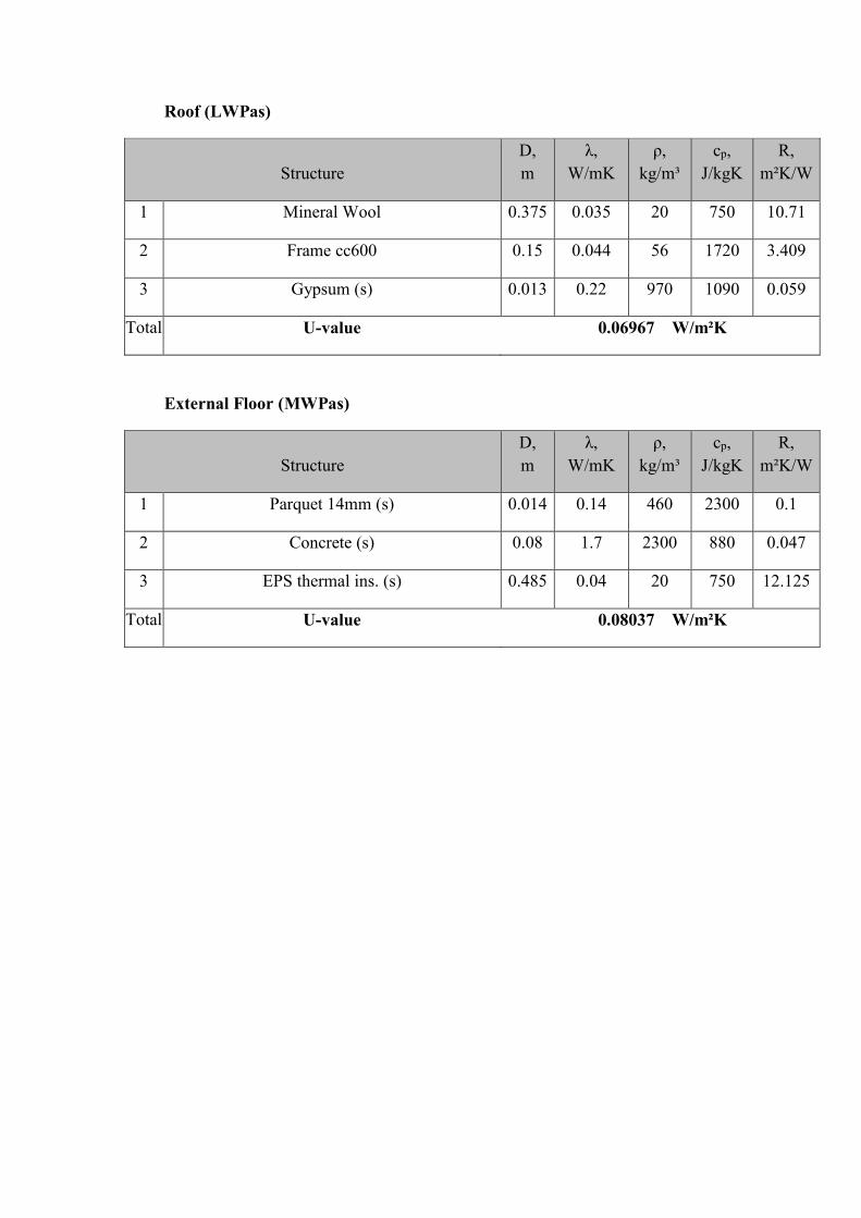
Roof (LWPas)
Structure
D,
m
λ,
W/mK
ρ,
kg/m³
cp,
J/kgK
R,
m²K/W
1 Mineral Wool 0.375 0.035 20 750 10.71
2 Frame cc600 0.15 0.044 56 1720 3.409
3 Gypsum (s) 0.013 0.22 970 1090 0.059
Total U-value 0.06967 W/m²K
External Floor (MWPas)
Structure
D,
m
λ,
W/mK
ρ,
kg/m³
cp,
J/kgK
R,
m²K/W
1 Parquet 14mm (s) 0.014 0.14 460 2300 0.1
2 Concrete (s) 0.08 1.7 2300 880 0.047
3 EPS thermal ins. (s) 0.485 0.04 20 750 12.125
Total U-value 0.08037 W/m²K
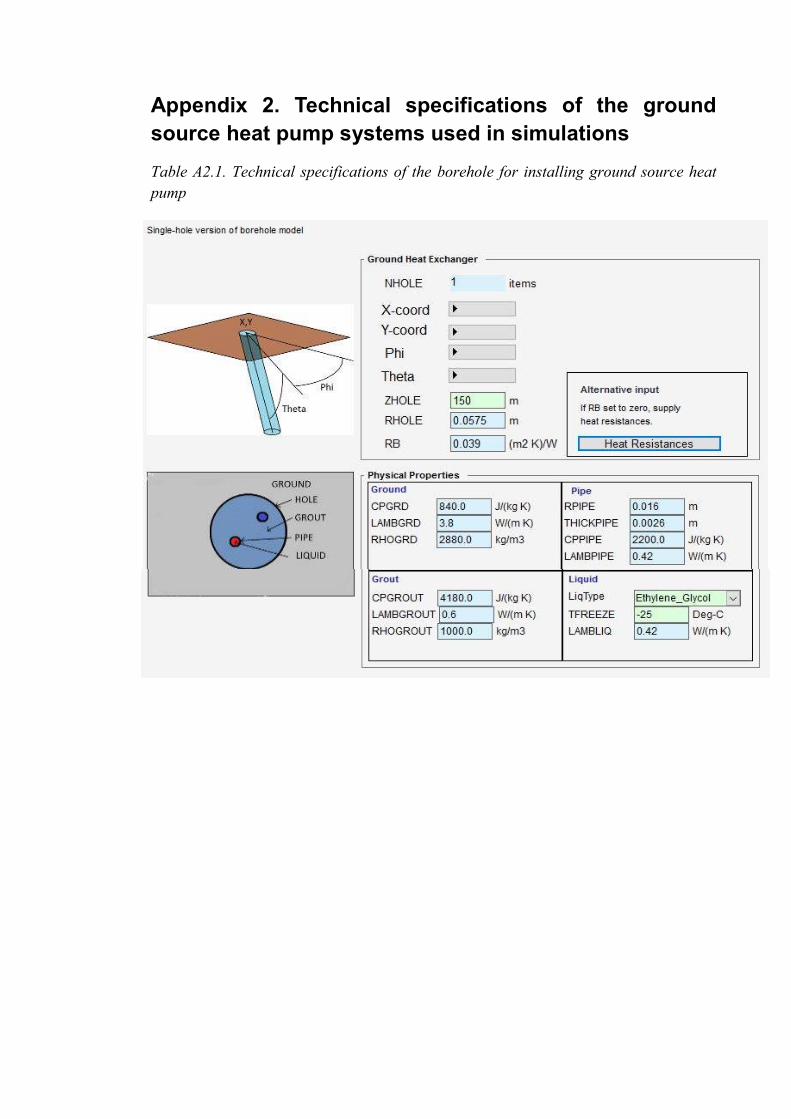
Appendix 2. Technical specifications of the ground
source heat pump systems used in simulations
Table A2.1. Technical specifications of the borehole for installing ground source heat
pump
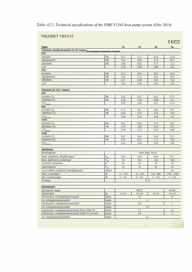
Table A2.2. Technical specifications of the NIBE F1345 heat pump system (Nibe 2014).
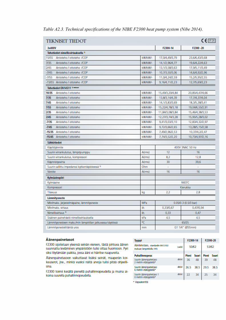
Table A2.3. Technical specifications of the NIBE F2300 heat pump system (Nibe 2014).

Table A2.4. Technical specifications of the Mitsubishi CAHV P500YA-HPB heat pump
system (Mitsubishi electric).
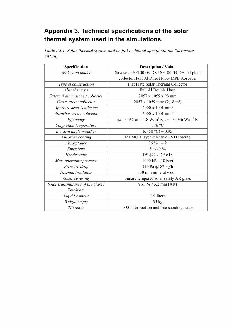
Appendix 3. Technical specifications of the solar
thermal system used in the simulations.
Table A3.1. Solar thermal system and its full technical specifications (Savosolar
2014b).
Specification Description / Value
Make and model Savosolar SF100-03-DS / SF100-03-DE flat plate
collector, Full Al Direct Flow MPE Absorber
Type of construction Flat Plate Solar Thermal Collector
Absorber type Full Al Double Harp
External dimensions / collector 2057 x 1059 x 98 mm
Gross area / collector 2057 x 1059 mm2 (2,18 m2)
Aperture area / collector 2000 x 1001 mm2
Absorber area / collector 2000 x 1001 mm2
Efficiency η0 = 0,92, a1 = 1,8 W/m2 K, a2 = 0,036 W/m2 K
Stagnation temperature 176 °C
Incident angle modifier K (50 °C) = 0,95
Absorber coating MEMO 3 layer selective PVD coating
Absorptance 96 % +/- 2
Emissivity 5 +/- 2 %
Header tube DS ϕ22 / DE ϕ18
Max. operating pressure 1000 kPa (10 bar)
Pressure drop 910 Pa @ 82 kg/h
Thermal insulation 50 mm mineral wool
Glass covering Sunarc tempered solar safety AR glass
Solar transmittance of the glass /
Thickness
96,1 % / 3,2 mm (AR)
Liquid content 1,9 liters
Weight empty 35 kg
Tilt angle 0-90° for rooftop and free standing setup

Figure A3.2. Dimensions of the solar thermal collectors (Savosolar 2014b).
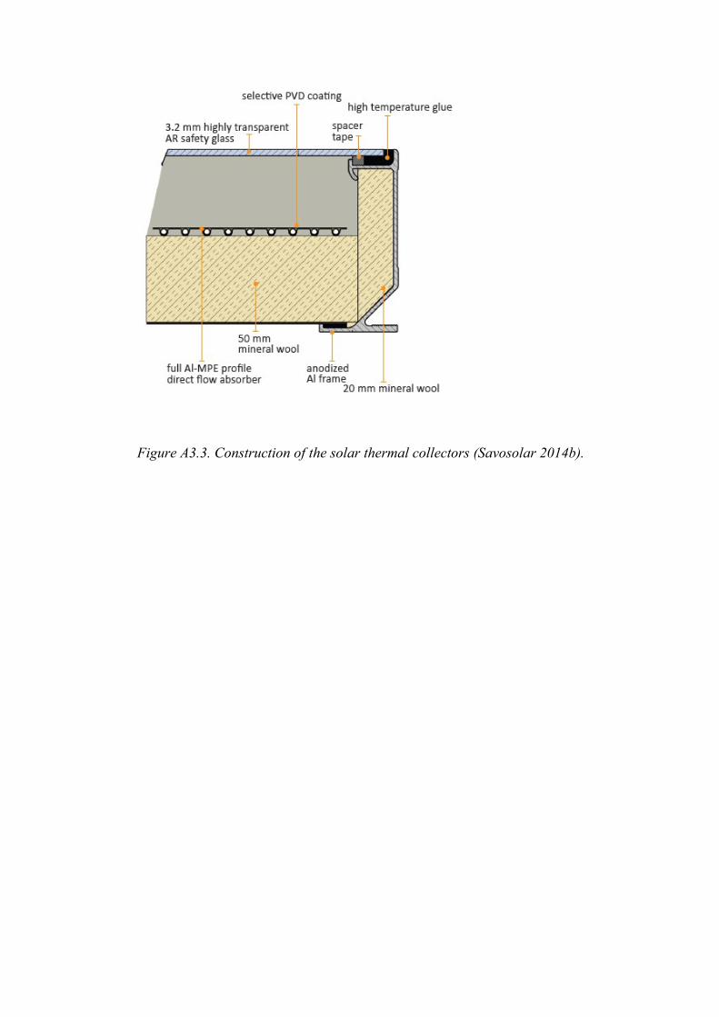
Figure A3.3. Construction of the solar thermal collectors (Savosolar 2014b).
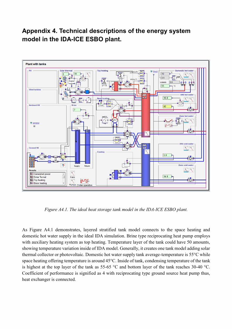
Appendix 4. Technical descriptions of the energy system
model in the IDA-ICE ESBO plant.
Figure A4.1. The ideal heat storage tank model in the IDA-ICE ESBO plant.
As Figure A4.1 demonstrates, layered stratified tank model connects to the space heating and
domestic hot water supply in the ideal IDA simulation. Brine type reciprocating heat pump employs
with auxiliary heating system as top heating. Temperature layer of the tank could have 50 amounts,
showing temperature variation inside of IDA model. Generally, it creates one tank model adding solar
thermal collector or photovoltaic. Domestic hot water supply tank average-temperature is 55°C while
space heating offering temperature is around 45°C. Inside of tank, condensing temperature of the tank
is highest at the top layer of the tank as 55-65 °C and bottom layer of the tank reaches 30-40 °C.
Coefficient of performance is signified as 4 with reciprocating type ground source heat pump thus,
heat exchanger is connected.

Appendix 5. Life Cycle Cost analysis used in the optimization
result.
Table A5.1 Electricity price based on information of 2012 by HVAC research team in Aalto Univ.
Finish VAT Electricity tax
(c/kWh)
Company margin
(c/kWh)
Distribution cost
(c/kWh)
Feed-in tariff
(c/kWh)
24% 2.79372 0.3 3.98 8.35
Table A5.2 Price of the hot water storage tank
Height
(m)
Diameter
(m)
Volume
(m3)
Price
(€)
Unit price
(€/m3)
2.050 0.650 0.68 1819.00 2675.36
2.050 0.800 1.03 2199.00 2135.12
2.050 0.950 1.45 2305.00 1587.09
2.100 1.050 1.82 2579.00 1419.00
2.150 1.250 2.64 3285.00 1245.68
2.250 1.400 3.46 3649.00 1054.06
2.250 1.500 3.97 3339.00 840.20
2.300 1.600 4.62 3539.00 765.67
2.350 1.800 5.98 4799.00 802.91