optimal stochastic control, stochastic …touzi/fields-ln.pdfstochastic control, namely stochastic...
TRANSCRIPT
OPTIMAL STOCHASTIC CONTROL,
STOCHASTIC TARGET PROBLEMS,
AND BACKWARD SDE
Nizar [email protected]
Ecole Polytechnique ParisDepartement de Mathematiques Appliquees
Chapter 12 by Agnes TOURIN
May 2010

2
Contents
1 Conditional Expectation and Linear Parabolic PDEs 111.1 Stochastic differential equations . . . . . . . . . . . . . . . . . . . 111.2 Markov solutions of SDEs . . . . . . . . . . . . . . . . . . . . . . 161.3 Connection with linear partial differential equations . . . . . . . 16
1.3.1 Generator . . . . . . . . . . . . . . . . . . . . . . . . . . . 161.3.2 Cauchy problem and the Feynman-Kac representation . . 171.3.3 Representation of the Dirichlet problem . . . . . . . . . . 19
1.4 The Black-Scholes model . . . . . . . . . . . . . . . . . . . . . . . 201.4.1 The continuous-time financial market . . . . . . . . . . . 201.4.2 Portfolio and wealth process . . . . . . . . . . . . . . . . . 211.4.3 Admissible portfolios and no-arbitrage . . . . . . . . . . . 221.4.4 Super-hedging and no-arbitrage bounds . . . . . . . . . . 231.4.5 The no-arbitrage valuation formula . . . . . . . . . . . . . 241.4.6 PDE characterization of the Black-Scholes price . . . . . . 24
2 Stochastic Control and Dynamic Programming 272.1 Stochastic control problems in standard form . . . . . . . . . . . 272.2 The dynamic programming principle . . . . . . . . . . . . . . . . 30
2.2.1 A weak dynamic programming principle . . . . . . . . . . 302.2.2 Dynamic programming without measurable selection . . . 32
2.3 The dynamic programming equation . . . . . . . . . . . . . . . . 352.4 On the regularity of the value function . . . . . . . . . . . . . . . 38
2.4.1 Continuity of the value function for bounded controls . . 382.4.2 A deterministic control problem with non-smooth value
function . . . . . . . . . . . . . . . . . . . . . . . . . . . . 402.4.3 A stochastic control problem with non-smooth value func-
tion . . . . . . . . . . . . . . . . . . . . . . . . . . . . . . 41
3 Optimal Stopping and Dynamic Programming 433.1 Optimal stopping problems . . . . . . . . . . . . . . . . . . . . . 433.2 The dynamic programming principle . . . . . . . . . . . . . . . . 453.3 The dynamic programming equation . . . . . . . . . . . . . . . . 463.4 Regularity of the value function . . . . . . . . . . . . . . . . . . . 49
3.4.1 Finite horizon optimal stopping . . . . . . . . . . . . . . . 49
3

4
3.4.2 Infinite horizon optimal stopping . . . . . . . . . . . . . . 503.4.3 An optimal stopping problem with nonsmooth value . . . 53
4 Solving Control Problems by Verification 554.1 The verification argument for stochastic control problems . . . . 554.2 Examples of control problems with explicit solutions . . . . . . . 58
4.2.1 Optimal portfolio allocation . . . . . . . . . . . . . . . . . 584.2.2 Law of iterated logarithm for double stochastic integrals . 60
4.3 The verification argument for optimal stopping problems . . . . . 634.4 Examples of optimal stopping problems with explicit solutions . 65
4.4.1 Pertual American options . . . . . . . . . . . . . . . . . . 654.4.2 Finite horizon American options . . . . . . . . . . . . . . 66
5 Introduction to Viscosity Solutions 695.1 Intuition behind viscosity solutions . . . . . . . . . . . . . . . . . 695.2 Definition of viscosity solutions . . . . . . . . . . . . . . . . . . . 705.3 First properties . . . . . . . . . . . . . . . . . . . . . . . . . . . . 715.4 Comparison result and uniqueness . . . . . . . . . . . . . . . . . 74
5.4.1 Comparison of classical solutions in a bounded domain . . 755.4.2 Semijets definition of viscosity solutions . . . . . . . . . . 755.4.3 The Crandall-Ishii’s lemma . . . . . . . . . . . . . . . . . 765.4.4 Comparison of viscosity solutions in a bounded domain . 78
5.5 Comparison in unbounded domains . . . . . . . . . . . . . . . . . 805.6 Useful applications . . . . . . . . . . . . . . . . . . . . . . . . . . 835.7 Proof of the Crandall-Ishii’s lemma . . . . . . . . . . . . . . . . . 84
6 Dynamic Programming Equation in the Viscosity Sense 896.1 DPE for stochastic control problems . . . . . . . . . . . . . . . . 896.2 DPE for optimal stopping problems . . . . . . . . . . . . . . . . 956.3 A comparison result for obstacle problems . . . . . . . . . . . . . 97
7 Stochastic Target Problems 997.1 Stochastic target problems . . . . . . . . . . . . . . . . . . . . . . 99
7.1.1 Formulation . . . . . . . . . . . . . . . . . . . . . . . . . . 997.1.2 Geometric dynamic programming principle . . . . . . . . 1007.1.3 The dynamic programming equation . . . . . . . . . . . . 1027.1.4 Application: hedging under portfolio constraints . . . . . 107
7.2 Stochastic target problem with controlled probability of success . 1097.2.1 Reduction to a stochastic target problem . . . . . . . . . 1107.2.2 The dynamic programming equation . . . . . . . . . . . . 1117.2.3 Application: quantile hedging in the Black-Scholes model 112
8 Second Order Stochastic Target Problems 1198.1 Superhedging under Gamma constraints . . . . . . . . . . . . . . 119
8.1.1 Problem formulation . . . . . . . . . . . . . . . . . . . . . 1208.1.2 Hedging under upper Gamma constraint . . . . . . . . . . 122

5
8.1.3 Including the lower bound on the Gamma . . . . . . . . . 127
8.2 Second order target problem . . . . . . . . . . . . . . . . . . . . . 129
8.2.1 Problem formulation . . . . . . . . . . . . . . . . . . . . . 129
8.2.2 The geometric dynamic programming . . . . . . . . . . . 131
8.2.3 The dynamic programming equation . . . . . . . . . . . . 131
8.3 Superhedging under illiquidity cost . . . . . . . . . . . . . . . . . 138
9 Backward SDEs and Stochastic Control 141
9.1 Motivation and examples . . . . . . . . . . . . . . . . . . . . . . 141
9.1.1 The stochastic Pontryagin maximum principle . . . . . . 142
9.1.2 BSDEs and stochastic target problems . . . . . . . . . . . 144
9.1.3 BSDEs and finance . . . . . . . . . . . . . . . . . . . . . . 144
9.2 Wellposedness of BSDEs . . . . . . . . . . . . . . . . . . . . . . . 145
9.2.1 Martingale representation for zero generator . . . . . . . . 146
9.2.2 BSDEs with affine generator . . . . . . . . . . . . . . . . 146
9.2.3 The main existence and uniqueness result . . . . . . . . . 147
9.3 Comparison and stability . . . . . . . . . . . . . . . . . . . . . . 149
9.4 BSDEs and stochastic control . . . . . . . . . . . . . . . . . . . . 151
9.5 BSDEs and semilinear PDEs . . . . . . . . . . . . . . . . . . . . 153
9.6 Appendix: essential supremum . . . . . . . . . . . . . . . . . . . 154
10 Quadratic backward SDEs 157
10.1 A priori estimates and uniqueness . . . . . . . . . . . . . . . . . . 157
10.1.1 A priori estimates for bounded Y . . . . . . . . . . . . . . 158
10.1.2 Some propeties of BMO martingales . . . . . . . . . . . . 159
10.1.3 Uniqueness . . . . . . . . . . . . . . . . . . . . . . . . . . 159
10.2 Existence . . . . . . . . . . . . . . . . . . . . . . . . . . . . . . . 161
10.2.1 Existence for small final condition . . . . . . . . . . . . . 161
10.2.2 Existence for bounded final condition . . . . . . . . . . . 163
10.3 Portfolio optimization under constraints . . . . . . . . . . . . . . 166
10.3.1 Problem formulation . . . . . . . . . . . . . . . . . . . . . 166
10.3.2 BSDE characterization . . . . . . . . . . . . . . . . . . . . 168
10.4 Interacting investors with performance concern . . . . . . . . . . 172
10.4.1 The Nash equilibrium problem . . . . . . . . . . . . . . . 172
10.4.2 The individual optimization problem . . . . . . . . . . . . 172
10.4.3 The case of linear constraints . . . . . . . . . . . . . . . . 174
10.4.4 Nash equilibrium under deterministic coefficients . . . . . 176
11 Probabilistic numerical methods for nonlinear PDEs 179
11.1 Discretization . . . . . . . . . . . . . . . . . . . . . . . . . . . . . 180
11.2 Convergence of the discrete-time approximation . . . . . . . . . . 182
11.3 Consistency, monotonicity and stability . . . . . . . . . . . . . . 184
11.4 The Barles-Souganidis monotone scheme . . . . . . . . . . . . . . 186

6
12 Introduction to Finite differences methods 18912.1 Overview of the Barles-Souganidis framework . . . . . . . . . . . 19012.2 First examples . . . . . . . . . . . . . . . . . . . . . . . . . . . . 192
12.2.1 The heat equation: the classic explicit and implicit schemes19212.2.2 The Black-Scholes-Merton PDE . . . . . . . . . . . . . . . 194
12.3 A nonlinear example: The Passport Option . . . . . . . . . . . . 19412.3.1 Problem formulation . . . . . . . . . . . . . . . . . . . . . 19412.3.2 Finite Difference approximation . . . . . . . . . . . . . . . 19512.3.3 Howard algorithm . . . . . . . . . . . . . . . . . . . . . . 197
12.4 The Bonnans-Zidani [7] approximation . . . . . . . . . . . . . . . 19712.5 Working in a finite domain . . . . . . . . . . . . . . . . . . . . . 19812.6 Variational Inequalities and splitting methods . . . . . . . . . . . 199
12.6.1 The American option . . . . . . . . . . . . . . . . . . . . 199

Introduction
These notes have been prepared for the graduate course tought at the FieldsInstitute, Toronto, during the Thematic program on quantitative finance whichwas held from January to June, 2010.
I would like to thank all participants to these lectures. It was a pleasure forme to share my experience on this subject with the excellent audience that wasoffered by this special research semester. In particular, their remarks and com-ments helped to improve parts of this document, and to correct some mistakes.
My special thanks go to Bruno Bouchard, Mete Soner and Agnes Tourinwho accepted to act as guest lecturers within this course. These notes havealso benefitted from the discussions with them, and some parts are based on myprevious work with Bruno and Mete.
These notes benefitted from careful reading by Matheus Grasselli and TomSalisbury. I greatly appreciate their help and hope there are not many mistakesleft.
I would like to express all my thanks to Matheus Grasselli, Tom Hurd, TomSalisbury, and Sebastian Jaimungal for the warm hospitality at the Fields Insti-tute, and their regular attendance to my lectures.
These lectures present the modern approach to stochastic control problemswith a special emphasis on the application in financial mathematics. For ped-agogical reason, we restrict the scope of the course to the control of diffusionprocesses, thus ignoring the presence of jumps.
We first review the main tools from stochastic analysis: Brownian motionand the corresponding stochastic integration theory. This already introducesto the first connection with partial differential equations (PDE). Indeed, byIto’s formula, a linear PDE pops up as the infinitesimal counterpart of thetower property. Conversely, given a nicely behaved smooth solution, the so-called Feynman-Kac formula provides a stochastic representation in terms of aconditional expectation.
We then introduce the class of standard stochastic control problems whereone wishes to maximize the expected value of some gain functional. The firstmain task is to derive an original weak dynamic programming principle whichavoids the heavy measurable selection arguments in typical proofs of the dy-namic programming principle when no a priori regularity of the value function
7

8 CHAPTER 0. INTRODUCTION
is known. The infinitesimal counterpart of the dynamic programming princi-ple is now a nonlinear PDE which is called dynamic programming equation,or Hamilton-Jacobi-Bellman equation. The hope is that the dynamic program-ming equation provides a complete characterization of the problem, once com-plemented with appropriate boundary conditions. However, this requires strongsmoothness conditions, which can be seen to be violated in simple examples.
A parallel picture can be drawn for optimal stopping problems and, in fact,for the more general control and stopping problems. In these notes we do nottreat such mixed control problem, and we rather analyze separately these twoclasses of control problems. Here again, we derive the dynamic programmingprinciple, and the corresponding dynamic programming equation under strongsmoothness conditions. In the present case, the dynamic programming equationtakes the form of the obstacle problem in PDEs.
When the dynamic programming equation happens to have an explicit smoothsolution, the verification argument allows to verify whether this candidate in-deed coincides with the value function of the control problem. The verificationargument provides as a by-product an access to the optimal control, i.e. thesolution of the problem. But of course, such lucky cases are rare, and one shouldnot count on solving any stochastic control problem by verification.
In the absence of any general a priori regularity of the value function, thenext development of the theory is based on viscosity solutions. This beautifulnotion was introduced by Crandal and Lions, and provides a weak notion ofsolutions to second order degenerate elliptic PDEs. We review the main toolsfrom viscosity solutions which are needed in stochastic control. In particular,we provide a difficulty-incremental presentation of the comparison result (i.e.maximum principle) which implies uniqueness.
We next show that the weak dynamic programming equation implies that thevalue function is a viscosity solution of the corresponding dynamic programmingequation in a wide generality. In particular, we do not assume that the controlsare bounded. We emphasize that in the present setting, there is no aprioriregularity of the value function needed to derive the dynamic programmingequation: we only need it to be locally bounded ! Given the general uniquenessresults, viscosity solutions provide a powerful tool for the characterization ofstochastic control and optimal stopping problems.
The remaining part of the lectures focus on the more recent literature onstochastic control, namely stochastic target problems. These problems are moti-vated by the superhedging problem in financial mathematics. Various extensionshave been studied in the literature. We focus on a particular setting where theproofs are simplified while highlighting the main ideas.
The use of viscosity solutions is crucial for the treatment of stochastic targetproblems. Indeed, deriving any a priori regularity seems to be a very difficulttask. Moreover, by writing formally the corresponding dynamic programmingequation and guessing an explicit solution (in some lucky case), there is noknown direct verification argument as in standard stochastic control problems.Our approach is then based on a dynamic programming principle suited to thisclass of problems, and called geometric dynamic programming principle, due to

9
a further extension of stochastic target problems to front propagation problemsin differential geometry. The geometric programming principle allows to obtaina dynamic programming equation in the sense of viscosity solutions. We providesome examples where the analysis of the dynamic programming equation leadsto a complete solution of the problem.
We also present an interesting extension to stochastic target problems withcontrolled probability of success. A remarkable trick allows to reduce theseproblems to standard stochastic target problems. By using this methodology,we show how one can solve explicitly the problem of quantile hedging whichwas previously solved by Follmer and Leukert [21] by duality methods in thestandard linear case in financial mathematics.
A further extension of stochastic target problems consists in involving thequadratic variation of the control process in the controlled state dynamics.These problems are motivated by examples from financial mathematics relatedto market illiquidity, and are called second order stochastic target problems. Wefollow the same line of arguments by formulating a suitable geometric dynamicprogramming principle, and deriving the corresponding dynamic programmingequation in the sense of viscosity solutions. The main new difficuly here is todeal with the short time asymptotics of double stochastic integrals.
The final part of the lectures explores a special type of stochastic targetproblems in the non-Markov framework. This leads to the theory of backwardstochastic differential equations (BSDE) which was introduced by Pardoux andPeng [33]. Here, in contrast to stochastic target problems, we insist on theexistence of a solution to the stochastic target problem. We provide the mainexistence, uniqueness, stability and comparison results. We also establish theconnection with stochastic control problems. We finally show the connectionwith semilinear PDEs in the Markov case.
The extension of the theory of BSDEs to the case where the generator isquadratic in the control variable is very important in view of the applicationsto portfolio optimization problems. However, the existence and uniqueness cannot be addressed as simply as in the Lipschitz case. The first existence anduniqueness results were established by Kobylanski [27] by adapting to the non-Markov framework techniques developed in the PDE literature. Instead of thishilghly technical argument, we report the beautiful argument recently developedby Tevzadze [39], and provide applications in financial mathematics.
The final chapter is dedicated to numerical methods for nonlinear PDEs.We provide a complete proof of convergence based on the Barles-Souganidismotone scheme method. The latter is a beautiful and simple argument whichexploits the stability of viscosity solutions. Stronger results are provided in thesemilinear case by using techniques from BSDEs.
Finally, I should like to expressall my love to my family:
Christine, our sons Ali and Heni, and our doughter Lilia,who accompanied me during this visit to Toronto,

10 CHAPTER 0. INTRODUCTION
all my thanks to them for their patience while I was preparing these notes,and all my apologies for my absence even when I was physically present...

Chapter 1
Conditional Expectationand Linear ParabolicPDEs
Throughout this chapter, (Ω,F ,F, P ) is a filtered probability space with filtra-tion F = Ft, t ≥ 0 satisfying the usual conditions. Let W = Wt, t ≥ 0 bea Brownian motion valued in Rd, defined on (Ω,F ,F, P ).
Throughout this chapter, a maturity T > 0 will be fixed. By H2, we denotethe collection of all progressively measurble processes φ with appropriate (finite)
dimension such that E[∫ T
0|φt|2dt
]<∞.
1.1 Stochastic differential equations
In this section, we recall the basic tools from stochastic differential equations
dXt = bt(Xt)dt+ σt(Xt)dWt, t ∈ [0, T ], (1.1)
where T > 0 is a given maturity date. Here, b and σ are F⊗B(Rn)-progressivelymeasurable functions from [0, T ] × Ω × Rn to Rn and MR(n, d), respectively.In particular, for every fixed x ∈ Rn, the processes bt(x), σt(x), t ∈ [0, T ] areF−progressively measurable.
Definition 1.1. A strong solution of (1.1) is an F−progressively measurable
process X such that∫ T
0(|bt(Xt)|+ |σt(Xt)|2)dt <∞, a.s. and
Xt = X0 +
∫ t
0
bs(Xs)ds+
∫ t
0
σs(Xs)dWs, t ∈ [0, T ].
Let us mention that there is a notion of weak solutions which relaxes someconditions from the above definition in order to allow for more general stochas-tic differential equations. Weak solutions, as opposed to strong solutions, are
11

12 CHAPTER 1. CONDITIONAL EXPECTATION AND LINEAR PDEs
defined on some probabilistic structure (which becomes part of the solution),and not necessarily on (Ω,F ,F,P,W ). Thus, for a weak solution we search for aprobability structure (Ω, F , F, P, W ) and a process X such that the requirementof the above definition holds true. Obviously, any strong solution is a weaksolution, but the opposite claim is false.
The main existence and uniqueness result is the following.
Theorem 1.2. Let X0 ∈ L2 be a r.v. independent of W . Assume that theprocesses b.(0) and σ.(0) are in H2, and that for some K > 0:
|bt(x)− bt(y)|+ |σt(x)− σt(y)| ≤ K|x− y| for all t ∈ [0, T ], x, y ∈ Rn.
Then, for all T > 0, there exists a unique strong solution of (1.1) in H2. More-over,
E[supt≤T|Xt|2
]≤ C
(1 + E|X0|2
)eCT , (1.2)
for some constant C = C(T,K) depending on T and K.
Proof. We first establish the existence and uniqueness result, then we prove theestimate (1.2).Step 1 For a constant c > 0, to be fixed later, we introduce the norm
‖φ‖H2c
:= E
[∫ T
0
e−ct|φt|2dt
]1/2
for every φ ∈ H2.
Clearly , the norms ‖.‖H2 and ‖.‖H2c
on the Hilbert space H2 are equivalent.Consider the map U on H2 by:
U(X)t := X0 +
∫ t
0
bs(Xs)ds+
∫ t
0
σs(Xs)dWs, 0 ≤ t ≤ T.
By the Lipschitz property of b and σ in the x−variable and the fact thatb.(0), σ.(0) ∈ H2, it follows that this map is well defined on H2. In orderto prove existence and uniqueness of a solution for (1.1), we shall prove thatU(X) ∈ H2 for all X ∈ H2 and that U is a contracting mapping with respect tothe norm ‖.‖H2
cfor a convenient choice of the constant c > 0.
1- We first prove that U(X) ∈ H2 for all X ∈ H2. To see this, we decompose:
‖U(X)‖2H2 ≤ 3T‖X0‖2L2 + 3TE
[∫ T
0
∣∣∣∣∫ t
0
bs(Xs)ds
∣∣∣∣2 dt]
+3E
[∫ T
0
∣∣∣∣∫ t
0
σs(Xs)dWs
∣∣∣∣2 dt]
By the Lipschitz-continuity of b and σ in x, uniformly in t, we have |bt(x)|2 ≤K(1 + |bt(0)|2 + |x|2) for some constant K. We then estimate the second term

1.1. Stochastic differential equations 13
by:
E
[∫ T
0
∣∣∣∣∫ t
0
bs(Xs)ds
∣∣∣∣2 dt]≤ KTE
[∫ T
0
(1 + |bt(0)|2 + |Xs|2)ds
]<∞,
since X ∈ H2, and b(., 0) ∈ L2([0, T ]).As, for the third term, we use the Doob maximal inequality together with
the fact that |σt(x)|2 ≤ K(1 + |σt(0)|2 + |x|2), a consequence of the Lipschitzproperty on σ:
E
[∫ T
0
∣∣∣∣∫ t
0
σs(Xs)dWs
∣∣∣∣2 dt]≤ TE
[maxt≤T
∣∣∣∣∫ t
0
σs(Xs)dWs
∣∣∣∣2 dt]
≤ 4TE
[∫ T
0
|σs(Xs)|2ds
]
≤ 4TKE
[∫ T
0
(1 + |σs(0)|2 + |Xs|2)ds
]<∞.
2- To see that U is a contracting mapping for the norm ‖.‖H2c, for some convenient
choice of c > 0, we consider two process X,Y ∈ H2 with X0 = Y0, and weestimate that:
E |U(X)t − U(Y )t|2
≤ 2E∣∣∣∣∫ t
0
(bs(Xs)− bs(Ys)) ds∣∣∣∣2 + 2E
∣∣∣∣∫ t
0
(σs(Xs)− σs(Ys)) dWs
∣∣∣∣2= 2E
∣∣∣∣∫ t
0
(bs(Xs)− bs(Ys)) ds∣∣∣∣2 + 2E
∫ t
0
|σs(Xs)− σs(Ys)|2 ds
≤ 2tE∫ t
0
|bs(Xs)− bs(Ys)|2 ds+ 2E∫ t
0
|σs(Xs)− σs(Ys)|2 ds
≤ 2(T + 1)K
∫ t
0
E |Xs − Ys|2 ds.
Hence, ‖U(X)− U(Y )‖c ≤2K(T + 1)
c‖X − Y ‖c, and therefore U is a contract-
ing mapping for sufficiently large c.Step 2 We next prove the estimate (1.2). We shall alleviate the notation writ-ing bs := bs(Xs) and σs := σs(Xs). We directly estimate:
E[supu≤t|Xu|2
]= E
[supu≤t
∣∣∣∣X0 +
∫ u
0
bsds+
∫ u
0
σsdWs
∣∣∣∣2]
≤ 3
(E|X0|2 + tE
[∫ t
0
|bs|2ds]
+ E
[supu≤t
∣∣∣∣∫ u
0
σsdWs
∣∣∣∣2])
≤ 3
(E|X0|2 + tE
[∫ t
0
|bs|2ds]
+ 4E[∫ t
0
|σs|2ds])
14 CHAPTER 1. CONDITIONAL EXPECTATION AND LINEAR PDEs
where we used the Doob’s maximal inequality. Since b and σ are Lipschitz-continuous in x, uniformly in t and ω, this provides:
E[supu≤t|Xu|2
]≤ C(K,T )
(1 + E|X0|2 +
∫ t
0
E[supu≤s|Xu|2
]ds
)and we conclude by using the Gronwall lemma. ♦
The following exercise shows that the Lipschitz-continuity condition on thecoefficients b and σ can be relaxed. We observe that further relaxation of thisassumption is possible in the one-dimensional case, see e.g. Karatzas and Shreve[24].
Exercise 1.3. In the context of this section, assume that the coefficients µand σ are locally Lipschitz and linearly growing in x, uniformly in (t, ω). By alocalization argument, prove that strong existence and uniqueness holds for thestochastic differential equation (1.1).
In addition to the estimate (1.2) of Theorem 1.2, we have the followingflow continuity results of the solution of the SDE. In order to emphasize thedependence on the initial date, we denote by Xt,x
s , s ≥ t the solution of theSDE (1.1) with initial condition Xt,x
t = x.
Theorem 1.4. Let the conditions of Theorem 1.2 hold true, and consider some(t, x) ∈ [0, T )× Rn with t ≤ t′ ≤ T .(i) There is a constant C such that:
E[
supt≤s≤t′
∣∣Xt,xs −Xt,x′
s |2∣∣] ≤ CeCt
′|x− x′|2. (1.3)
(ii) Assume further that B := supt<t′≤T (t′ − t)−1E∫ t′t
(|br(0)|2 + |σr(0)|2
)dr <
∞. Then for all t′ ∈ [t, T ]:
E[
supt′≤s≤T
∣∣Xt,xs −Xt′,x
s |2∣∣] ≤ CeCT (B + |x|2)|t′ − t|. (1.4)
Proof. (i) To simplify the notations, we set Xs := Xt,xs and X ′s := Xt,x′
s for alls ∈ [t, T ]. We also denote δx := x− x′, δX := X −X ′, δb := b(X)− b(X ′) andδσ := σ(X)− σ(X ′). We first decompose:
|δXs|2 ≤ 3
(|δx|2 +
∣∣∣ ∫ s
t
δbudu∣∣∣2 +
∣∣∣ ∫ s
t
δσudWu
∣∣∣2)≤ 3
(|δx|2 + (s− t)
∫ s
t
∣∣δbu∣∣2du+
∫ s
t
δσudWu
∣∣∣2) .

1.1. Stochastic differential equations 15
Then, it follows from the Doob maximal inequality and the Lipschitz propertyof the coefficients b and σ that:
h(t′) := E[
supt≤s≤t′
|δXs|2]≤ 3
(|δx|2 + (s− t)
∫ s
t
E∣∣δbu∣∣2du+ 4
∫ s
t
E∣∣δσu∣∣2du)
≤ 3
(|δx|2 +K2(t′ + 4)
∫ s
t
E|δXu|2du)
≤ 3
(|δx|2 +K2(t′ + 4)
∫ s
t
h(u)du
).
Then the required estimate follows from the Gronwall inequality.
(ii) We next prove (1.4). We again simplify the notation by setting Xs := Xt,xs ,
s ∈ [t, T ], and X ′s := Xt′,xs , s ∈ [t′, T ]. We also denote δt := t′−t, δX := X−X ′,
δb := b(X)−b(X ′) and δσ := σ(X)−σ(X ′). Then following the same argumentsas in the previous step, we obtain for all u ∈ [t′, T ]:
h(u) := E[
supt′≤s≤u
|δXs|2]≤ 3
(E|Xt′ − x|2 +K2(T + 4)
∫ u
t′E|δXr|2dr
)≤ 3
(E|Xt′ − x|2 +K2(T + 4)
∫ u
t′h(r)dr
)(1.5)
Observe that
E|Xt′ − x|2 ≤ 2
(E∣∣∣ ∫ t′
t
br(Xr)dr∣∣∣2 + E
∣∣∣ ∫ t′
t
σr(Xr)dr∣∣∣2)
≤ 2
(T
∫ t′
t
E|br(Xr)|2dr +
∫ t′
t
E|σr(Xr)|2dr
)
≤ 6(T + 1)
∫ t′
t
(K2E|Xr − x|2 + |x|2 + E|br(0)|2
)dr
≤ 6(T + 1)(
(t′ − t)(|x|2 +B) +K2
∫ t′
t
E|Xr − x|2dr).
By the Gronwall inequality, this shows that
E|Xt′ − x|2 ≤ C(|x|2 +B)|t′ − t|eC(t′−t).
Plugging this estimate in (1.5), we see that:
h(u) ≤ 3
(C(|x|2 +B)|t′ − t|eC(t′ − t) +K2(T + 4)
∫ u
t′h(r)dr
), (1.6)
and the required estimate follows from the Gronwall inequality. ♦

16 CHAPTER 1. CONDITIONAL EXPECTATION AND LINEAR PDEs
1.2 Markov solutions of SDEs
In this section, we restrict the coefficients b and σ to be deterministic functionsof (t, x). In this context, we write
bt(x) = b(t, x), σt(x) = σ(t, x) for t ∈ [0, T ], x ∈ Rn,
where b and σ are continuous functions, Lipschitz in x uniformly in t. Let Xt,x.
denote the solution of the stochastic differential equation
Xt,xs = x+
∫ s
t
b(u,Xt,x
u
)du+
∫ s
t
σ(u,Xt,x
u
)dWu s ≥ t
The two following properties are obvious:
• Clearly, Xt,xs = F (t, x, s, (W. −Wt)t≤u≤s) for some deterministic function
F .
• For t ≤ u ≤ s: Xt,xs = X
u,Xt,xus . This follows from the pathwise uniqueness,
and holds also when u is a stopping time.
With these observations, we have the following Markov property for the solutionsof stochastic differential equations.
Proposition 1.5. (Markov property) For all 0 ≤ t ≤ s:
E [Φ (Xu, t ≤ u ≤ s) |Ft] = E [Φ (Xu, t ≤ u ≤ s) |Xt]
for all bounded function Φ : C([t, s]) −→ R.
1.3 Connection with linear partial differentialequations
1.3.1 Generator
Let Xt,xs , s ≥ t be the unique strong solution of
Xt,xs = x+
∫ s
t
b(u,Xt,xu )du+
∫ s
t
σ(u,Xt,xu )dWu, s ≥ t,
where µ and σ satisfy the required condition for existence and uniqueness of astrong solution.
For a function f : Rn −→ R, we define the function Af by
Af(t, x) = limh→0
E[f(Xt,xt+h)]− f(x)
hif the limit exists.
Clearly, Af is well-defined for all bounded C2− function with bounded deriva-tives and
Af(t, x) = b(t, x) ·Df(x) +1
2Tr[σσT(t, x)D2f(x)
], (1.7)

1.3. Connection with PDE 17
where Df and D2f denote the gradient and Hessian of f , respectively. (Exercise!). The linear differential operator A is called the generator of X. It turns outthat the process X can be completely characterized by its generator or, moreprecisely, by the generator and the corresponding domain of definition.
As the following result shows, the generator provides an intimate connectionbetween conditional expectations and linear partial differential equations.
Proposition 1.6. Assume that the function (t, x) 7−→ v(t, x) := E[g(Xt,x
T
]is
C1,2 ([0, T )× Rn). Then v solves the partial differential equation:
∂v
∂t+Av = 0 and v(T, .) = g.
Proof. Given (t, x), let τ1 := T ∧ infs > t : |Xt,xs − x| ≥ 1. By the law of
iterated expectation together with the Markov property of the process X, itfollows that
v(t, x) = E[v(s ∧ τ1, Xt,x
s∧τ1)].
Since v ∈ C1,2([0, T ),Rn), we may apply Ito’s formula, and we obtain by takingexpectations:
0 = E[∫ s∧τ1
t
(∂v
∂t+Av
)(u,Xt,x
u )du
]+E
[∫ s∧τ1
t
∂v
∂x(u,Xt,x
s ) · σ(u,Xt,xu )dWu
]= E
[∫ s∧τ1
t
(∂v
∂t+Av
)(u,Xt,x
u )du
],
where the last equality follows from the boundedness of (u,Xt,xu ) on [t, s∧τ1]. We
now send s t, and the required result follows from the dominated convergencetheorem. ♦
1.3.2 Cauchy problem and the Feynman-Kac representa-tion
In this section, we consider the following linear partial differential equation
∂v∂t +Av − k(t, x)v + f(t, x) = 0, (t, x) ∈ [0, T )× Rdv(T, .) = g
(1.8)
where A is the generator (1.7), g is a given function from Rd to R, k and f arefunctions from [0, T ] × Rd to R, b and σ are functions from [0, T ] × Rd to Rdand and MR(d, d), respectively. This is the so-called Cauchy problem.
For example, when k = f ≡ 0, b ≡ 0, and σ is the identity matrix, the abovepartial differential equation reduces to the heat equation.

18 CHAPTER 1. CONDITIONAL EXPECTATION AND LINEAR PDEs
Our objective is to provide a representation of this purely deterministic prob-lem by means of stochastic differential equations. We then assume that b andσ satisfy the conditions of Theorem 1.2, namely that
b, σ Lipschitz in x uniformly in t,
∫ T
0
(|b(t, 0)|2 + |σ(t, 0)|2
)dt <∞.(1.9)
Theorem 1.7. Let the coefficients b, σ be continuous and satisfy (1.9). Assumefurther that the function k is uniformly bounded from below, and f has quadraticgrowth in x uniformly in t. Let v be a C1,2
([0, T ),Rd
)solution of (1.8) with
quadratic growth in x uniformly in t. Then
v(t, x) = E
[∫ T
t
βt,xs f(s,Xt,xs )ds+ βt,xT g
(Xt,xT
)], t ≤ T, x ∈ Rd ,
where Xt,xs , s ≥ t is the solution of the SDE 1.1 with initial data Xt,x
t = x,
and βt,xs := e−∫ stk(u,Xt,xu )du for t ≤ s ≤ T .
Proof. We first introduce the sequence of stopping times
τn := T ∧ infs > t :
∣∣Xt,xs − x
∣∣ ≥ n ,and we oberve that τn −→ T P−a.s. Since v is smooth, it follows from Ito’sformula that for t ≤ s < T :
d(βt,xs v
(s,Xt,x
s
))= βt,xs
(−kv +
∂v
∂t+Av
)(s,Xt,x
s
)ds
+βt,xs∂v
∂x
(s,Xt,x
s
)· σ(s,Xt,x
s
)dWs
= βt,xs
(−f(s,Xt,x
s )ds+∂v
∂x
(s,Xt,x
s
)· σ(s,Xt,x
s
)dWs
),
by the PDE satisfied by v in (1.8). Then:
E[βt,xτn v
(τn, X
t,xτn
)]− v(t, x)
= E[∫ τn
t
βt,xs
(−f(s,Xs)ds+
∂v
∂x
(s,Xt,x
s
)· σ(s,Xt,x
s
)dWs
)].
Now observe that the integrands in the stochastic integral is bounded by def-inition of the stopping time τn, the smoothness of v, and the continuity of σ.Then the stochastic integral has zero mean, and we deduce that
v(t, x) = E[∫ τn
t
βt,xs f(s,Xt,x
s
)ds+ βt,xτn v
(τn, X
t,xτn
)]. (1.10)

1.3. Connection with PDE 19
Since τn −→ T and the Brownian motion has continuous sample paths P−a.s.it follows from the continuity of v that, P−a.s.∫ τn
t
βt,xs f(s,Xt,x
s
)ds+ βt,xτn v
(τn, X
t,xτn
)n→∞−→
∫ T
t
βt,xs f(s,Xt,x
s
)ds+ βt,xT v
(T,Xt,x
T
)=
∫ T
t
βt,xs f(s,Xt,x
s
)ds+ βt,xT g
(Xt,xT
) (1.11)
by the terminal condition satisfied by v in (1.8). Moreover, since k is boundedfrom below and the functions f and v have quadratic growth in x uniformly int, we have∣∣∣∣∫ τn
t
βt,xs f(s,Xt,x
s
)ds+ βt,xτn v
(τn, X
t,xτn
)∣∣∣∣ ≤ C
(1 + max
t≤T|Xt|2
).
By the estimate stated in the existence and uniqueness theorem 1.2, the latterbound is integrable, and we deduce from the dominated convergence theoremthat the convergence in (1.11) holds in L1(P), proving the required result bytaking limits in (1.10). ♦
The above Feynman-Kac representation formula has an important numericalimplication. Indeed it opens the door to the use of Monte Carlo methods in orderto obtain a numerical approximation of the solution of the partial differentialequation (1.8). For sake of simplicity, we provide the main idea in the casef = k = 0. Let
(X(1), . . . , X(k)
)be an iid sample drawn in the distribution of
Xt,xT , and compute the mean:
vk(t, x) :=1
k
k∑i=1
g(X(i)
).
By the Law of Large Numbers, it follows that vk(t, x) −→ v(t, x) P−a.s. More-over the error estimate is provided by the Central Limit Theorem:
√k (vk(t, x)− v(t, x))
k→∞−→ N(0,Var
[g(Xt,xT
)])in distribution,
and is remarkably independent of the dimension d of the variable X !
1.3.3 Representation of the Dirichlet problem
Let D be an open subset of Rd. The Dirichlet problem is to find a function usolving:
Au− ku+ f = 0 on D and u = g on ∂D, (1.12)

20 CHAPTER 1. CONDITIONAL EXPECTATION AND LINEAR PDEs
where ∂D denotes the boundary of D, and A is the generator of the processX0,x defined as the unique strong solution of the stochastic differential equation
X0,xt = x+
∫ t
0
µ(s,X0,xs )ds+
∫ t
0
σ(s,X0,xs )dWs, t ≥ 0.
Similarly to the the representation result of the Cauchy problem obtained inTheorem 1.7, we have the following representation result for the Dirichlet prob-lem.
Theorem 1.8. Let u be a C2−solution of the Dirichlet problem (1.12). Assumethat k is nonnegative, and
E[τxD] <∞, x ∈ Rd, where τxD := inft ≥ 0 : X0,x
t 6∈ D.
Then, we have the representation:
u(x) = E
[g(X0,xτxD
)e−∫ τxD0 k(Xs)ds +
∫ τxD
0
f(X0,xt
)e−∫ t0k(Xs)dsdt
].
Exercise 1.9. Provide a proof of Theorem 1.8 by imitating the arguments inthe proof of Theorem 1.7.
1.4 The Black-Scholes model
1.4.1 The continuous-time financial market
Let T be a finite horizon, and (Ω,F ,P) be a complete probability space sup-porting a Brownian motion W = (W 1
t , . . . ,Wdt ), 0 ≤ t ≤ T with values in Rd.
We denote by F = FW = Ft, 0 ≤ t ≤ T the canonical augmented filtration ofW , i.e. the canonical filtration augmented by zero measure sets of FT .
We consider a financial market consisting of d+ 1 assets :
(i) The first asset S0 is locally riskless, and is defined by
S0t = exp
(∫ t
0
rudu
), 0 ≤ t ≤ T,
where rt, t ∈ [0, T ] is a non-negative adapted processes with∫ T
0rtdt <∞ a.s.,
and represents the instantaneous interest rate.
(ii) The d remaining assets Si, i = 1, . . . , d, are risky assets with priceprocesses defined by the dynamics
dSitSit
= µitdt+
d∑j=1
σi,jt dW jt , t ∈ [0, T ],

1.3. Connection with PDE 21
for 1 ≤ i ≤ d, where µ, σ are F−adapted processes with∫ T
0|µit|dt+
∫ T0|σi,jt |2dt <
∞ for all i, j = 1, . . . , d. It is convenient to use the matrix notations to representthe dynamics of the price vector S = (S1, . . . , Sd):
dSt = St ? (µtdt+ σtdWt) , t ∈ [0, T ],
where, for two vectors x, y ∈ Rd, we denote x ? y the vector of Rd with compo-nents (x ? y)i = xiyi, i = 1, . . . , d, and µ, σ are the Rd−vector with componentsµi’s, and the MR(d, d)−matrix with entries σi,j .
We assume that the MR(d, d)−matrix σt is invertible for every t ∈ [0, T ]a.s., and we introduce the process
λt := σ−1t (µt − rt1) , 0 ≤ t ≤ T,
called the risk premium process. Here 1 is the vector of ones in Rd. We shallfrequently make use of the discounted processes
St :=StS0t
= St exp
(−∫ t
0
rudu
),
Using the above matrix notations, the dynamics of the process S are given by
dSt = St ?((µt − rt1)dt+ σtdWt
)= St ? σt (λtdt+ dWt) .
1.4.2 Portfolio and wealth process
A portfolio strategy is an F−adapted process π = πt, 0 ≤ t ≤ T with valuesin Rd. For 1 ≤ i ≤ n and 0 ≤ t ≤ T , πit is the amount (in Euros) invested inthe risky asset Si.
We next recall the self-financing condition in the present framework. Let Xπt
denote the portfolio value, or wealth, process at time t induced by the portfoliostrategy π. Then, the amount invested in the non-risky asset is Xπ
t −∑ni=1 π
it
= Xπt − πt · 1.
Under the self-financing condition, the dynamics of the wealth process isgiven by
dXπt =
n∑i=1
πitSit
dSit +Xπt − πt · 1S0t
dS0t .
Let Xπ be the discounted wealth process
Xπt := Xπ
t exp
(−∫ t
0
rudu
), 0 ≤ t ≤ T.
Then, by an immediate application of Ito’s formula, we see that
dXt = πt · σt (λtdt+ dWt) , 0 ≤ t ≤ T, (1.13)

22 CHAPTER 1. CONDITIONAL EXPECTATION AND LINEAR PDEs
where πt := e−∫ t0ruduπt. We still need to place further technical conditions on
π, at least in order for the above wealth process to be well-defined as a stochasticintegral.
Before this, let us observe that, assuming that the risk premium processsatisfies the Novikov condition:
E[e
12
∫ T0|λt|2dt
]< ∞,
it follows from the Girsanov theorem that the process
Bt := Wt +
∫ t
0
λudu , 0 ≤ t ≤ T , (1.14)
is a Brownian motion under the equivalent probability measure
Q := ZT · P on FT where ZT := exp
(−∫ T
0
λu · dWu −1
2
∫ T
0
|λu|2du
).
In terms of the Q Brownian motion B, the discounted price process satisfies
dSt = St ? σtdBt, t ∈ [0, T ],
and the discounted wealth process induced by an initial capital X0 and a port-folio strategy π can be written in
Xπt = X0 +
∫ t
0
πu · σudBu, for 0 ≤ t ≤ T. (1.15)
Definition 1.10. An admissible portfolio process π = πt, t ∈ [0, T ] is an
F−progressively measurable process such that∫ T
0|σTt πt|2dt < ∞, a.s. and the
corresponding discounted wealth process is bounded from below by a Q−martingale
Xπt ≥Mπ
t , 0 ≤ t ≤ T, for some Q−martingale Mπ.
The collection of all admissible portfolio processes will be denoted by A.
The lower bound Mπ, which may depend on the portfolio π, has the interpre-tation of a finite credit line imposed on the investor. This natural generalizationof the more usual constant credit line corresponds to the situation where thetotal credit available to an investor is indexed by some financial holding, such asthe physical assets of the company or the personal home of the investor, used ascollateral. From the mathematical viewpoint, this condition is needed in orderto exclude any arbitrage opportunity, and will be justified in the subsequentsubsection.
1.4.3 Admissible portfolios and no-arbitrage
We first define precisely the notion of no-arbitrage.

1.3. Connection with PDE 23
Definition 1.11. We say that the financial market contains no arbitrage op-portunities if for any admissible portfolio process θ ∈ A,
X0 = 0 and XθT ≥ 0 P− a.s. implies Xθ
T = 0 P− a.s.
The purpose of this section is to show that the financial market describedabove contains no arbitrage opportunities. Our first observation is that, by thevery definition of the probability measure Q, the discounted price process Ssatisfies:
the processSt, 0 ≤ t ≤ T
is a Q− local martingale. (1.16)
For this reason, Q is called a risk neutral measure, or an equivalent local mar-tingale measure, for the price process S.
We also observe that the discounted wealth process satisfies:
Xπ is a Q−local martingale for every π ∈ A, (1.17)
as a stochastic integral with respect to the Q−Brownian motion B.
Theorem 1.12. The continuous-time financial market described above containsno arbitrage opportunities, i.e. for every π ∈ A:
X0 = 0 and XπT ≥ 0 P− a.s. =⇒ Xπ
T = 0 P− a.s.
Proof. For π ∈ A, the discounted wealth process Xπ is a Q−local martingalebounded from below by a Q−martingale. Then Xπ is a Q−super-martingale.
In particular, EQ[XπT
]≤ X0 = X0. Recall that Q is equivalent to P and S0
is strictly positive. Then, this inequality shows that, whenever Xπ0 = 0 and
XπT ≥ 0 P−a.s. (or equivalently Q−a.s.), we have Xπ
T = 0 Q−a.s. and thereforeXπT = 0 P−a.s. ♦
1.4.4 Super-hedging and no-arbitrage bounds
Let G be an FT−measurable random variable representing the payoff of a deriva-tive security with given maturity T > 0. The super-hedging problem consists infinding the minimal initial cost so as to be able to face the payment G withoutrisk at the maturity of the contract T :
V (G) := inf X0 ∈ R : XπT ≥ G P− a.s. for some π ∈ A .
Remark 1.13. Notice that V (G) depends on the reference measure P only bymeans of the corresponding null sets. Therefore, the super-hedging problem isnot changed if P is replaced by any equivalent probability measure.
We now show that, under the no-arbitrage condition, the super-hedgingproblem provides no-arbitrage bounds on the market price of the derivative se-curity.

24 CHAPTER 1. CONDITIONAL EXPECTATION AND LINEAR PDEs
Assume that the buyer of the contingent claim G has the same access tothe financial market than the seller. Then V (G) is the maximal amount thatthe buyer of the contingent claim contract is willing to pay. Indeed, if the sellerrequires a premium of V (G) + 2ε, for some ε > 0, then the buyer would notaccept to pay this amount as he can obtain at least G by trading on the financialmarket with initial capital V (G) + ε.
Now, since selling of the contingent claim G is the same as buying the con-tingent claim −G, we deduce from the previous argument that
−V (−G) ≤ market price of G ≤ V (G). (1.18)
1.4.5 The no-arbitrage valuation formula
We denote by p(G) the market price of a derivative security G.
Theorem 1.14. Let G be an FT−measurabel random variable representing thepayoff of a derivative security at the maturity T > 0, and recall the notation
G := G exp(−∫ T
0rtdt
). Assume that EQ[|G|] <∞. Then
p(G) = V (G) = EQ[G].
Moreover, there exists a portfolio π∗ ∈ A such that Xπ∗
0 = p(G) and Xπ∗
T = G,a.s., that is π∗ is a perfect replication strategy.
Proof. 1- We first prove that V (G) ≥ EQ[G]. Let X0 and π ∈ A be such thatXπT ≥ G, a.s. or, equivalently, Xπ
T ≥ G a.s. Notice that Xπ is a Q−super-martingale, as a Q−local martingale bounded from below by a Q−martingale.Then X0 = X0 ≥ EQ[Xπ
T ] ≥ EQ[G].2- We next prove that V (G) ≤ EQ[G]. Define the Q−martingale Yt := EQ[G|Ft]and observe that FW = FB . Then, it follows from the martingale representa-
tion theorem that Yt = Y0 +∫ T
0φt · dBt for some F−adapted process φ with∫ T
0|φt|2dt <∞ a.s. Setting π∗ := (σT)−1φ, we see that
π∗ ∈ A and Y0 +
∫ T
0
π∗ · σtdBt = G P− a.s.
which implies that Y0 ≥ V (G) and π∗ is a perfect hedging stratgey for G,starting from the initial capital Y0.3- From the previous steps, we have V (G) = EQ[G]. Applying this result to −G,we see that V (−G) = −V (G), so that the no-arbitrage bounds (1.18) imply thatthe no-arbitrage market price of G is given by V (G). ♦
1.4.6 PDE characterization of the Black-Scholes price
In this subsection, we specialize further the model to the case where the riskysecurities price processes are Markov diffusions defined by the stochastic differ-ential equations:
dSt = St ?(r(t, St)dt+ σ(t, St)dBt
).

1.3. Connection with PDE 25
Here (t, s) 7−→ s ? r(t, s) and (t, s) 7−→ s ? σ(t, s) are Lipschitz-continuous func-tions from R+ × [0,∞)d to Rd and Sd, successively. We also consider a Vanilladerivative security defined by the payoff
G = g(ST ),
where g : [0,∞)d → R is a measurable function bounded from below. Byan immediate extension of the results from the previous subsection, the no-arbitrage price at time t of this derivative security is given by
V (t, St) = EQ[e−∫ Ttr(u,Su)dug(ST )|Ft
]= EQ
[e−∫ Ttr(u,Su)dug(ST )|St
],
where the last equality follows from the Markov property of the process S.Assuming further that g has linear growth, it follows that V has linear growthin s uniformly in t. Since V is defined by a conditional expectation, it is expectedto satisfy the linear PDE:
−∂tV − rs ? DV −1
2Tr[(s ? σ)2D2V
]+ rV = 0. (1.19)
More precisely, if V ∈ C1,2(R+,Rd), then V is a classical solution of (1.19) andsatisfies the final condition V (T, .) = g. Coversely, if the PDE (1.19) combinedwith the final condition v(T, .) = g has a classical solution v with linear growth,then v coincides with the derivative security price V .

26 CHAPTER 1. CONDITIONAL EXPECTATION AND LINEAR PDEs

Chapter 2
Stochastic Controland Dynamic Programming
In this chapter, we assume that the filtration F is the P−augmentation of thecanonical filtration of the Brownian motion W . This restriction is only neededin order to simplify the presentation of the proof of the dynamic programmingprinciple. We will also denote by
S := [0, T )× Rd where T ∈ [0,∞].
The set S is called the parabolic interior of the state space. We will denote byS := cl(S) its closure, i.e. S = [0, T ]× Rd for finite T , and S = S for T =∞.
2.1 Stochastic control problems in standard form
Control processes. Given a subset U of Rk, we denote by U the set of all pro-gressively measurable processes ν = νt, t < T valued in U . The elements ofU are called control processes.
Controlled Process. Let
b : (t, x, u) ∈ S× U −→ b(t, x, u) ∈ Rd
and
σ : (t, x, u) ∈ S× U −→ σ(t, x, u) ∈MR(n, d)
be two continuous functions satisfying the conditions
|b(t, x, u)− b(t, y, u)|+ |σ(t, x, u)− σ(t, y, u)| ≤ K |x− y|, (2.1)
|b(t, x, u)|+ |σ(t, x, u)| ≤ K (1 + |x|+ |u|). (2.2)
27

28 CHAPTER 2. STOCHASTIC CONTROL, DYNAMIC PROGRAMMING
for some constant K independent of (t, x, y, u). For each control process ν ∈ U ,we consider the controlled stochastic differential equation :
dXt = b(t,Xt, νt)dt+ σ(t,Xt, νt)dWt. (2.3)
If the above equation has a unique solution X, for a given initial data, thenthe process X is called the controlled process, as its dynamics is driven by theaction of the control process ν.
We shall be working with the following subclass of control processes :
U0 := U ∩H2, (2.4)
where H2 is the collection of all progressively measurable processes with finiteL2(Ω × [0, T ))−norm. Then, for every finite maturity T ′ ≤ T , it follows fromthe above uniform Lipschitz condition on the coefficients b and σ that
E
[∫ T ′
0
(|b|+ |σ|2
)(s, x, νs)ds
]<∞ for all ν ∈ U0, x ∈ Rd,
which guarantees the existence of a controlled process on the time interval [0, T ′]for each given initial condition and control. The following result is an immediateconsequence of Theorem 1.2.
Theorem 2.1. Let ν ∈ U0 be a control process, and ξ ∈ L2(P) be an F0−measurablerandom variable. Then, there exists a unique F−adapted process Xν satisfying(2.3) together with the initial condition Xν
0 = ξ. Moreover for every T > 0,there is a constant C > 0 such that
E[
sup0≤s≤t
|Xνs |2]< C(1 + E[|ξ|2])eCt for all t ∈ [0, T ). (2.5)
Gain functional. Let
f, k : [0, T )× Rd × U −→ R and g : Rd −→ R
be given functions. We assume that f, k are continuous and ‖k−‖∞ < ∞ (i.e.max(−k, 0) is uniformly bounded). Moreover, we assume that f and g satisfythe quadratic growth condition :
|f(t, x, u)|+ |g(x)| ≤ K(1 + |u|+ |x|2),
for some constant K independent of (t, x, u). We define the gain function J on[0, T ]× Rd × U by :
J(t, x, ν) := E
[∫ T
t
βν(t, s)f(s,Xt,x,νs , νs)ds+ βν(t, T )g(Xt,x,ν
T )1T<∞
],
when this expression is meaningful, where
βν(t, s) := e−∫ stk(r,Xt,x,νr ,νr)dr,

2.1. Standard stochastic control 29
and Xt,x,νs , s ≥ t is the solution of (2.3) with control process ν and initial
condition Xt,x,νt = x.
Admissible control processes. In the finite horizon case T < ∞, the quadraticgrowth condition on f and g together with the bound on k− ensure that J(t, x, ν)is well-defined for all control process ν ∈ U0. We then define the set of admissiblecontrols in this case by U0.
More attention is needed for the infinite horizon case. In particular, thediscount term k needs to play a role to ensure the finiteness of the integral. Inthis setting the largest set of admissible control processes is given by
U0 :=ν ∈ U : E
[ ∫ ∞0
βν(t, s)(1+|Xt,x,ν
s |2+|νs)|)ds]<∞ for all x
when T =∞.
The stochastic control problem. Consider the optimization problem
V (t, x) := supν∈U0
J(t, x, ν) for (t, x) ∈ S.
Our main concern is to describe the local behavior of the value function Vby means of the so-called dynamic programming equation, or Hamilton-Jacobi-Bellman equation. We continue with some remarks.
Remark 2.2. (i) If V (t, x) = J(t, x, νt,x), we call νt,x an optimal control forthe problem V (t, x).
(ii) The following are some interesting subsets of controls :
- a process ν ∈ U0 which is adapted to the natural filtration FX of theassociated state process is called feedback control,
- a process ν ∈ U0 which can be written in the form νs = u(s,Xs) for somemeasurable map u from [0, T ] × Rd into U , is called Markovian control;notice that any Markovian control is a feedback control,
- the deterministic processes of U0 are called open loop controls.
(iii) Suppose that T < ∞, and let (Y,Z) be the controlled processes definedby
dYs = Zsf(s,Xs, νs)ds and dZs = −Zsk(s,Xs, νs)ds ,
and define the augmented state process X := (X,Y, Z). Then, the abovevalue function V can be written in the form :
V (t, x) = V (t, x, 0, 1) ,
where x = (x, y, z) is some initial data for the augmented state process X,
V (t, x) := Et,x[g(XT )
]and g(x, y, z) := y + g(x)z .
Hence the stochastic control problem V can be reduced without loss ofgenerality to the case where f = k ≡ 0. We shall appeal to this reducedform whenever convenient for the exposition.

30 CHAPTER 2. STOCHASTIC CONTROL, DYNAMIC PROGRAMMING
(iv) Consider the case T < ∞. In view of the previous Remark (iii), we mayassume without loss of generality that f = k = 0. Consider the valuefunction
V (t, x) := supν∈Ut
E[g(Xt,x,ν
T )], (2.6)
differing from V by the restriction of the control processes to
Ut := ν ∈ U0 : ν independent of Ft . (2.7)
Since Ut ⊂ U0, it is obvious that V ≤ V . We claim that
V = V, (2.8)
so that both problems are indeed equivalent. To see this, fix (t, x) ∈ S andν ∈ U0. Then, ν can be written as a measurable function of the canonicalprocess ν((ωs)0≤s≤t, (ωs−ωt)t≤s≤T ), where, for fixed (ωs)0≤s≤t, the mapν(ωs)0≤s≤t : (ωs − ωt)t≤s≤T 7→ ν((ωs)0≤s≤t, (ωs − ωt)t≤s≤T ) can be viewedas a control independent on Ft. Using the independence of the incrementsof the Brownian motion, together with Fubini’s Lemma, it thus followsthat
J(t, x; ν) =
∫E[g(X
t,x,ν(ωs)0≤s≤tT )
]dP((ωs)0≤s≤t)
≤∫V (t, x)dP((ωs)0≤s≤t) = V (t, x).
By arbitrariness of ν ∈ U0, this implies that V (t, x) ≥ V (t, x).
(v) The extension of the previous Remark (iv) to the infinite horizon case isalso immediate.
2.2 The dynamic programming principle
2.2.1 A weak dynamic programming principle
The dynamic programming principle is the main tool in the theory of stochasticcontrol. In these notes, we shall prove rigorously a weak version of the dy-namic programming which will be sufficient for the derivation of the dynamicprogramming equation. We denote:
V∗(t, x) := lim inf(t′,x′)→(t,x)
V (t′, x′) and V ∗(t, x) := lim sup(t′,x′)→(t,x)
V (t′, x′),
for all (t, x) ∈ S. We also recall the subset of controls Ut introduced in (2.7)above.

2.2. Dynamic programming principle 31
Theorem 2.3. Assume that V is locally bounded. Let (t, x) ∈ S be fixed. Letθν , ν ∈ Ut be a family of finite stopping times independent of Ft with valuesin [t, T ]. Then:
V (t, x) ≤ supν∈Ut
E
[∫ θν
t
βν(t, s)f(s,Xt,x,νs , νs)ds+ βν(t, θν)V∗(θ
ν , Xt,x,νθν )
].
Assume further that g is lower-semicontinuous and Xνt,x1[t,θν ] is L∞−bounded
for all ν ∈ Ut. Then
V (t, x) ≥ supν∈Ut
E
[∫ θν
t
βν(t, s)f(s,Xt,x,νs , νs)ds+ βν(t, θν)V ∗(θν , Xt,x,ν
θν )
].
We shall provide an intuitive justification of this result after the followingcomments. A rigorous proof is reported in Section 2.2.2 below.
(i) If V is continuous, then V = V∗ = V ∗, and the above weak dynamic pro-gramming principle reduces to the classical dynamic programming princi-ple:
V (t, x) = supν∈U
Et,x
[∫ θ
t
β(t, s)f(s,Xs, νs)ds+ β(t, θ)V (θ,Xθ)
].(2.9)
(ii) In the discrete-time framework, the dynamic programming principle (2.9)can be stated as follows :
V (t, x) = supu∈U
Et,x[f(t,Xt, u) + e−k(t+1,Xt+1,u)V (t+ 1, Xt+1)
].
Observe that the supremum is now taken over the subset U of the finitedimensional space Rk. Hence, the dynamic programming principle allowsto reduce the initial maximization problem, over the subset U of the in-finite dimensional set of Rk−valued processes, into a finite dimensionalmaximization problem. However, we are still facing an infinite dimen-sional problem since the dynamic programming principle relates the valuefunction at time t to the value function at time t+ 1.
(iii) In the context of the above discrete-time framework with finite horizonT <∞, notice that the dynamic programming principle suggests the fol-lowing backward algorithm to compute V as well as the associated optimalstrategy (when it exists). Since V (T, ·) = g is known, the above dynamicprogramming principle can be applied recursively in order to deduce thevalue function V (t, x) for every t.
(iv) In the continuous time setting, there is no obvious counterpart to theabove backward algorithm. But, as the stopping time θ approaches t,the above dynamic programming principle implies a special local behaviorfor the value function V . When V is known to be smooth, this will beobtained by means of Ito’s formula.

32 CHAPTER 2. STOCHASTIC CONTROL, DYNAMIC PROGRAMMING
(v) It is usually very difficult to determine a priori the regularity of V . Thesituation is even worse since there are many counter-examples showingthat the value function V can not be expected to be smooth in general;see Section 2.4. This problem is solved by appealing to the notion ofviscosity solutions, which provides a weak local characterization of thevalue function V .
(vi) Once the local behavior of the value function is characterized, we arefaced to the important uniqueness issue, which implies that V is com-pletely characterized by its local behavior together with some convenientboundary condition.
Intuitive justification of (2.9). Let us assume that V is continuous. Inparticular, V is measurable and V = V∗ = V ∗. Let V (t, x) denote the righthand-side of (2.9).
By the tower Property of the conditional expectation operator, it is easilychecked that
J(t, x, ν) = Et,x
[∫ θ
t
β(t, s)f(s,Xs, νs)ds+ β(t, θ)J(θ,Xθ, ν)
].
Since J(θ,Xθ, ν) ≤ V (θ,Xθ), this proves that V ≤ V . To prove the reverseinequality, let µ ∈ U and ε > 0 be fixed, and consider an ε−optimal control νε
for the problem V (θ,Xθ), i.e.
J(θ,Xθ, νε) ≥ V (θ,Xθ)− ε.
Clearly, one can choose νε = µ on the stochastic interval [t, θ]. Then
V (t, x) ≥ J(t, x, νε) = Et,x
[∫ θ
t
β(t, s)f(s,Xs, µs)ds+ β(t, θ)J(θ,Xθ, νε)
]
≥ Et,x
[∫ θ
t
β(t, s)f(s,Xs, µs)ds+ β(t, θ)V (θ,Xθ)
]− ε Et,x[β(t, θ)] .
This provides the required inequality by the arbitrariness of µ ∈ U and ε > 0.♦
Exercise. Where is the gap in the above sketch of the proof ?
2.2.2 Dynamic programming without measurable selec-tion
In this section, we provide a rigorous proof of Theorem 2.3. Notice that, wehave no information on whether V is measurable or not. Because of this, the

2.2. Dynamic programming principle 33
right-hand side of the classical dynamic programming principle (2.9) is not evenknown to be well-defined.
The formulation of Theorem 2.3 avoids this measurability problem sinceV∗ and V ∗ are lower- and upper-semicontinuous, respectively, and thereforemeasurable. In addition, it allows to avoid the typically heavy technicalitiesrelated to measurable selection arguments needed for the proof of the classicaldynamic programming principle (2.9) after a convenient relaxation of the controlproblem, see e.g. El Karoui and Jeanblanc [16].
Proof of Theorem 2.3 For simplicity, we consider the finite horizon caseT < ∞, so that, without loss of generality, we assume f = k = 0, See Remark2.2 (iii). The extension to the infinite horizon framework is immediate.1. Let ν ∈ Ut be arbitrary and set θ := θν . Then:
E[g(Xt,x,νT
)|Fθ]
(ω) = J(θ(ω), Xt,x,νθ (ω); νω),
where νω is obtained from ν by freezing its trajectory up to the stopping timeθ. Since, by definition, J(θ(ω), Xt,x,ν
θ (ω); νω) ≤ V ∗(θ(ω), Xt,x,νθ (ω)), it follows
from the tower property of conditional expectations that
E[g(Xt,x,νT
)]= E
[E[g(Xt,x,νT
)|Fθ]]≤ E
[V ∗(θ,Xt,x,ν
θ
)],
which provides the second inequality of Theorem 2.3 by the arbitrariness ofν ∈ Ut.2. Let ε > 0 be given, and consider an arbitrary function
ϕ : S −→ R such that ϕ upper-semicontinuous and V ≥ ϕ.
2.a. There is a family (ν(s,y),ε)(s,y)∈S ⊂ U0 such that:
ν(s,y),ε ∈ Us and J(s, y; ν(s,y),ε) ≥ V (s, y)− ε, for every (s, y) ∈ S.(2.10)
Since g is lower-semicontinuous and has quadratic growth, it follows from Theo-rem 2.1 that the function (t′, x′) 7→ J(t′, x′; ν(s,y),ε) is lower-semicontinuous, forfixed (s, y) ∈ S. Together with the upper-semicontinuity of ϕ, this implies thatwe may find a family (r(s,y))(s,y)∈S of positive scalars so that, for any (s, y) ∈ S,
ϕ(s, y)− ϕ(t′, x′) ≥ −ε and J(s, y; ν(s,y),ε)− J(t′, x′; ν(s,y),ε) ≤ εfor (t′, x′) ∈ B(s, y; r(s,y)),
(2.11)
where, for r > 0 and (s, y) ∈ S,
B(s, y; r) := (t′, x′) ∈ S : t′ ∈ (s− r, s), |x′ − y| < r . (2.12)
Note that we do not use here balls of the usual form Br(s, y). The fact thatt′ ≤ s for (t′, x′) ∈ B(s, y; r) will play an important role in Step 3 below.Clearly,
B(s, y; r) : (s, y) ∈ S, 0 < r ≤ r(s,y)
forms an open covering of
[0, T ) × Rd. It then follows from the Lindelof covering Theorem, see e.g. [15]

34 CHAPTER 2. STOCHASTIC CONTROL, DYNAMIC PROGRAMMING
Theorem 6.3 Chap. VIII, that we can find a countable sequence (ti, xi, ri)i≥1
of elements of S × R, with 0 < ri ≤ r(ti,xi) for all i ≥ 1, such that S ⊂T × Rd ∪ (∪i≥1B(ti, xi; ri)). Set A0 := T × Rd, C−1 := ∅, and define thesequence
Ai+1 := B(ti+1, xi+1; ri+1) \ Ci where Ci := Ci−1 ∪Ai, i ≥ 0.
With this construction, it follows from (2.10), (2.11), together with the fact thatV ≥ ϕ, that the countable family (Ai)i≥0 satisfies
(θ,Xt,x,νθ ) ∈ ∪i≥0Ai P− a.s., Ai ∩Aj = ∅ for i 6= j ∈ N,
and J(·; νi,ε) ≥ ϕ− 3ε on Ai for i ≥ 1,(2.13)
where νi,ε := ν(ti,xi),ε for i ≥ 1.2.b. We now prove the first inequality in Theorem 2.3. We fix ν ∈ Ut andθ ∈ T t[t,T ]. Set An := ∪0≤i≤nAi, n ≥ 1. Given ν ∈ Ut, we define for s ∈ [t, T ]:
νε,ns := 1[t,θ](s)νs + 1(θ,T ](s)(νs1(An)c(θ,X
t,x,νθ ) +
n∑i=1
1Ai(θ,Xt,x,νθ )νi,εs
).
Notice that (θ,Xt,x,νθ ) ∈ Ai ∈ F tθ, and therefore νε,n ∈ Ut. By the definition
of the neighbourhood (2.12), notice that θ = θ ∧ ti ≤ ti on (θ,Xνt,x(θ)) ∈ Ai.
Then, it follows from (2.13) that:
E[g(Xt,x,νε,n
T
)|Fθ]
1An(θ,Xt,x,ν
θ
)= V
(T,Xt,x,νε,n
T
)1A0
(θ,Xt,x,ν
θ
)+
n∑i=1
J(θ,Xt,x,νθ , νi,ε)1Ai
(θ,Xt,x,ν
θ
)≥
n∑i=0
(ϕ(θ,Xt,x,ν
θ − 3ε)1Ai
(θ,Xt,x,ν
θ
)=
(ϕ(θ,Xt,x,ν
θ )− 3ε)1An
(θ,Xt,x,ν
θ
),
which, by definition of V and the tower property of conditional expectations,implies
V (t, x) ≥ J(t, x, νε,n)
= E[E[g(Xt,x,νε,n
T
)|Fθ]]
≥ E[(ϕ(θ,Xt,x,ν
θ
)− 3ε
)1An
(θ,Xt,x,ν
θ
)]+E
[g(Xt,x,νT
)1(An)c
(θ,Xt,x,ν
θ
)].
Since g(Xt,x,νT
)∈ L1, it follows from the dominated convergence theorem that:
V (t, x) ≥ −3ε+ lim infn→∞
E[ϕ(θ,Xt,x,ν
θ )1An(θ,Xt,x,ν
θ
)]= −3ε+ lim
n→∞E[ϕ(θ,Xt,x,ν
θ )+1An(θ,Xt,x,ν
θ
)]− limn→∞
E[ϕ(θ,Xt,x,ν
θ )−1An(θ,Xt,x,ν
θ
)]= −3ε+ E
[ϕ(θ,Xt,x,ν
θ )],

2.3. Dynamic programming equation 35
where the last equality follows from the left-hand side of (2.13) and from themonotone convergence theorem, due to the fact that either E
[ϕ(θ,Xt,x,ν
θ )+]<
∞ or E[ϕ(θ,Xt,x,ν
θ )−]< ∞. By the arbitrariness of ν ∈ Ut and ε > 0, this
shows that:
V (t, x) ≥ supν∈Ut
E[ϕ(θ,Xt,x,ν
θ )]. (2.14)
3. It remains to deduce the first inequality of Theorem 2.3 from (2.14). Fixr > 0. It follows from standard arguments, see e.g. Lemma 3.5 in [35], thatwe can find a sequence of continuous functions (ϕn)n such that ϕn ≤ V∗ ≤ Vfor all n ≥ 1 and such that ϕn converges pointwise to V∗ on [0, T ] × Br(0).Set φN := minn≥N ϕn for N ≥ 1 and observe that the sequence (φN )N is non-decreasing and converges pointwise to V∗ on [0, T ] × Br(0). By (2.14) and themonotone convergence Theorem, we then obtain:
V (t, x) ≥ limN→∞
E[φN (θν , Xν
t,x(θν))]
= E[V∗(θ
ν , Xνt,x(θν))
].
♦
2.3 The dynamic programming equation
The dynamic programming equation is the infinitesimal counterpart of the dy-namic programming principle. It is also widely called the Hamilton-Jacobi-Bellman equation. In this section, we shall derive it under strong smoothnessassumptions on the value function. Let Sd be the set of all d × d symmetricmatrices with real coefficients, and define the map H : S× R× Rd × Sd by :
H(t, x, r, p, γ)
:= supu∈U
−k(t, x, u)r + b(t, x, u) · p+
1
2Tr[σσT(t, x, u)γ] + f(t, x, u)
.
We also need to introduce the linear second order operator Lu associated tothe controlled process βu(0, t)Xu
t , t ≥ 0 controlled by the constant controlprocess u :
Luϕ(t, x) := −k(t, x, u)ϕ(t, x) + b(t, x, u) ·Dϕ(t, x)
+1
2Tr[σσT(t, x, u)D2ϕ(t, x)
],
where D and D2 denote the gradient and the Hessian operators with respect tothe x variable. With this notation, we have by Ito’s formula:
βν(0, s)ϕ(s,Xνs )− βν(0, t)ϕ(t,Xν
t ) =
∫ s
t
βν(0, r) (∂t + Lνr )ϕ(r,Xνr )dr
+
∫ s
t
βν(0, r)Dϕ(r,Xνr ) · σ(r,Xν
r , νr)dWr
for every s ≥ t and smooth function ϕ ∈ C1,2([t, s],Rd) and each admissiblecontrol process ν ∈ U0.

36 CHAPTER 2. STOCHASTIC CONTROL, DYNAMIC PROGRAMMING
Proposition 2.4. Assume the value function V ∈ C1,2([0, T ),Rd), and let thecoefficients k(·, ·, u) and f(·, ·, u) be continuous in (t, x) for all fixed u ∈ U .Then, for all (t, x) ∈ S:
−∂tV (t, x)−H(t, x, V (t, x), DV (t, x), D2V (t, x)
)≥ 0. (2.15)
Proof. Let (t, x) ∈ S and u ∈ U be fixed and consider the constant controlprocess ν = u, together with the associated state process X with initial dataXt = x. For all h > 0, Define the stopping time :
θh := inf s > t : (s− t,Xs − x) 6∈ [0, h)× αB ,
where α > 0 is some given constant, and B denotes the unit ball of Rd. Noticethat θh −→ t, P−a.s. when h 0, and θh = h for h ≤ h(ω) sufficiently small.1. From the first inequality of the dynamic programming principle, togetherwith the continuity of V , it follows that :
0 ≤ Et,x
[βu(0, t)V (t, x)− βu(0, θh)V (θh, Xθh)−
∫ θh
t
βu(0, r)f(r,Xr, u)dr
]
= −Et,x
[∫ θh
t
βu(0, r)(∂tV + L·V + f)(r,Xr, u)dr
]
−Et,x
[∫ θh
t
βu(0, r)DV (r,Xr) · σ(r,Xr, u)dWr
],
the last equality follows from Ito’s formula and uses the crucial smoothnessassumption on V .2. Observe that β(0, r)DV (r,Xr) · σ(r,Xr, u) is bounded on the stochasticinterval [t, θh]. Therefore, the second expectation on the right hand-side of thelast inequality vanishes, and we obtain :
−Et,x
[1
h
∫ θh
t
βu(0, r)(∂tV + L·V + f)(r,Xr, u)dr
]≥ 0
We now send h to zero. The a.s. convergence of the random value inside theexpectation is easily obtained by the mean value Theorem; recall that θh = h
for sufficiently small h > 0. Since the random variable h−1∫ θhtβu(0, r)(L·V +
f)(r,Xr, u)dr is essentially bounded, uniformly in h, on the stochastic interval[t, θh], it follows from the dominated convergence theorem that :
−∂tV (t, x)− LuV (t, x)− f(t, x, u) ≥ 0.
By the arbitrariness of u ∈ U , this provides the required claim. ♦
We next wish to show that V satisfies the nonlinear partial differential equa-tion (2.16) with equality. This is a more technical result which can be proved bydifferent methods. We shall report a proof, based on a contradiction argument,which provides more intuition on this result, although it might be slightly longerthan the usual proof reported in standard textbooks.

2.3. Dynamic programming equation 37
Proposition 2.5. Assume V ∈ C1,2([0, T ),Rd) and H(., V.DV,D2V ) > −∞.Assume further that k is bounded and the function H is continuous. Then, forall (t, x) ∈ S:
−∂tV (t, x)−H(t, x, V (t, x), DV (t, x), D2V (t, x)
)≤ 0. (2.16)
Proof. Let (t0, x0) ∈ [0, T )× Rd be fixed, assume to the contrary that
∂tV (t0, x0) +H(t0, x0, V (t0, x0), DV (t0, x0), D2V (t0, x0)
)< 0, (2.17)
and let us work towards a contradiction.1. For a given parameter ε > 0, define the smooth function ϕ ≥ V by
ϕ(t, x) := V (t, x) + ε(|t− t0|2 + |x− x0|4
).
Then
(V − ϕ)(t0, x0) = 0, (DV −Dϕ)(t0, x0) = 0, (∂tV − ∂tϕ)(t0, x0) = 0,
and (D2V −D2ϕ)(t0, x0) = 0,
and it follows from the continuity of H and (2.17) that:
h(t, x) :=(∂tϕ+H(., ϕ,Dϕ,D2ϕ)
)(t, x) < 0 for (t, x) ∈ Nr, (2.18)
for some sufficiently small parameter r > 0, where Nr := (t0 − r, t0 + r) ×rB(t0, x0) ⊂ [−r, T ]× Rn.2. From the definition of ϕ, we have
−η := max∂Nr
(V − ϕ) < 0. (2.19)
For an arbitrary control process ν ∈ Ut0 , we define the stopping time
θν := inft > t0 : Xt0,x0,νt 6∈ Nr,
and we observe that(θν , Xt0,x0,ν
θν
)∈ ∂Nr by the pathwise continuity of the
controlled process. Then, it follows from (2.19) that:
ϕ(θν , Xt0,x0,ν
θν
)≥ η + V
(θν , Xt0,x0,ν
θν
). (2.20)
3. For notation simplicity, we set βνs := βν(t0, s). Since βνt0 = 1, it follows fromIto’s formula that:
V (t0, x0) = ϕ(t0, x0)
= E[βνθνϕ
(θν , Xt0,x0,ν
θν
)−∫ θν
t0
βνs(∂t + Lνs
)ϕ(s,Xt0,x0,ν
s
)ds]
≥ E[βνθνϕ
(θν , Xt0,x0,ν
θν
)+
∫ θν
t0
βνs(f(., νs)− h
)(s,Xt0,x0,ν
s
)ds]

38 CHAPTER 2. STOCHASTIC CONTROL, DYNAMIC PROGRAMMING
By the definition of h. Since(s,Xt0,x0,ν
s
)∈ Nr on [t0, θ
ν) it follows from (2.18)and (2.20) that:
V (t0, x0) ≥ ηE[βνθν ] + E[ ∫ θν
t0
βνs f(s,Xt0,x0,ν
s , νs)ds+ βνθνV
(θν , Xt0,x0,ν
θν
)]≥ ηe−r|k
+|∞ + E[ ∫ θν
t0
βνs f(s,Xt0,x0,ν
s , νs)ds+ βνθνV
(θν , Xt0,x0,ν
θν
)].
Since η > 0 does not depend on ν, it follows from the arbitrariness of ν ∈ Ut0and the continuity of V that the last inequality is in contradiction with thesecond inequality of the dynamic programming principle of Theorem (2.3). ♦
As a consequence of Propositions 2.4 and 2.5, we have the main result ofthis section :
Theorem 2.6. Let the conditions of Propositions 2.5 and 2.4 hold. Then, thevalue function V solves the Hamilton-Jacobi-Bellman equation
−∂tV −H(., V,DV,D2V
)= 0 on S. (2.21)
2.4 On the regularity of the value function
The purpose of this paragraph is to show that the value function should not beexpected to be smooth in general. We start by proving the continuity of thevalue function under strong conditions; in particular, we require the set U inwhich the controls take values to be bounded. We then give a simple examplein the deterministic framework where the value function is not smooth. Sinceit is well known that stochastic problems are “more regular” than deterministicones, we also give an example of stochastic control problem whose value functionis not smooth.
2.4.1 Continuity of the value function for bounded con-trols
For simplicity, we reduce the stochastic control problem to the case f = k ≡ 0,see Remark 2.2 (iii). We will also concentrate on the finite horizon case T <∞.The corresponding results in the infinite horizon case can be obtained by similararguments. Our main concern, in this section, is to show the standard argumentfor proving the continuity of the value function. Therefore, the following resultsassume strong conditions on the coefficients of the model in order to simplify theproofs. We first start by examining the value function V (t, ·) for fixed t ∈ [0, T ].
Proposition 2.7. Let f = k ≡ 0, T < ∞, and assume that g is Lipschitzcontinuous. Then:(i) V is Lipschitz in x, uniformly in t.
2.4. Regularity of the value function 39
(ii) Assume further that U is bounded. Then V is 12−Holder-continuous in t,
and there is a constant C > 0 such that:∣∣V (t, x)− V (t′, x)∣∣ ≤ C(1 + |x|)
√|t− t′|; t, t′ ∈ [0, T ], x ∈ Rd.
Proof. (i) For x, x′ ∈ Rd and t ∈ [0, T ), we first estimate that:
|V (t, x)− V (t, x′)| ≤ supν∈U0
E∣∣∣g (Xt,x,ν
T
)− g
(Xt,x′,νT
)∣∣∣≤ Const sup
ν∈U0
E∣∣∣Xt,x,ν
T −Xt,x′,νT
∣∣∣≤ Const |x− x′|,
where we used the Lipschitz-continuity of g together with the flow estimatesof Theorem 1.4, and the fact that the coefficients b and σ are Lipschitz in xuniformly in (t, u). This compltes the proof of the Lipschitz property of thevalue function V .(ii) To prove the Holder continuity in t, we shall use the dynamic programmingprinciple.
(ii-1) We first make the following important observation. A careful reviewof the proof of Theorem 2.3 reveals that, whenever the stopping times θν areconstant (i.e. deterministic), the dynamic programming principle holds truewith the semicontinuous envelopes taken only with respect to the x−variable.Since V was shown to be continuous in the first part of this proof, we deducethat:
V (t, x) = supν∈U0
E[V(t′, Xt,x,ν
t′
)](2.22)
for all x ∈ Rd, t < t′ ∈ [0, T ].(ii-2) Fix x ∈ Rd, t < t′ ∈ [0, T ]. By the dynamic programming principle
(2.22), we have :
|V (t, x)− V (t′, x)| =
∣∣∣∣ supν∈U0
E[V(t′, Xt,x,ν
t′
)]− V (t′, x)
∣∣∣∣≤ sup
ν∈U0
E∣∣V (t′, Xt,x,ν
t′
)− V (t′, x)
∣∣ .By the Lipschitz-continuity of V (s, ·) established in the first part of this proof,we see that :
|V (t, x)− V (t′, x)| ≤ Const supν∈U0
E∣∣Xt,x,ν
t′ − x∣∣ . (2.23)
We shall now prove that
supν∈U
E∣∣Xt,x,ν
t′ − x∣∣ ≤ Const (1 + |x|)|t− t′|1/2, (2.24)

40 CHAPTER 2. STOCHASTIC CONTROL, DYNAMIC PROGRAMMING
which provides the required (1/2)−Holder continuity in view of (2.23). Bydefinition of the process X, and assuming t < t′, we have
E∣∣Xt,x,ν
t′ − x∣∣2 = E
∣∣∣∣∣∫ t′
t
b(r,Xr, νr)dr +
∫ t′
t
σ(r,Xr, νr)dWr
∣∣∣∣∣2
≤ Const E
[∫ t′
t
|h(r,Xr, νr)|2 dr
]
where h := [b2 + σ2]1/2. Since h is Lipschitz-continuous in (t, x, u) and hasquadratic growth in x and u, this provides:
E∣∣Xt,x,ν
t′ − x∣∣2 ≤ Const
(∫ t′
t
(1 + |x|2 + |νr|2)dr +
∫ t′
t
E∣∣Xt,x,ν
r − x∣∣2 dr) .
Since the control process ν is uniformly bounded, we obtain by the Gronwalllemma the estimate:
E∣∣Xt,x,ν
t′ − x∣∣2 ≤ Const (1 + |x|)|t′ − t|, (2.25)
where the constant does not depend on the control ν. ♦
Remark 2.8. When f and/or k are non-zero, the conditions required on f andk in order to obtain the (1/2)−Holder continuity of the value function can bededuced from the reduction of Remark 2.2 (iii).
Remark 2.9. Further regularity results can be proved for the value functionunder convenient conditions. Typically, one can prove that LuV exists in thegeneralized sense, for all u ∈ U . This implies immediately that the result ofProposition 2.5 holds in the generalized sense. More technicalities are needed inorder to derive the result of Proposition 2.4 in the generalized sense. We referto [20], §IV.10, for a discussion of this issue and to Krylov [28] for the technicalproofs.
2.4.2 A deterministic control problem with non-smoothvalue function
Let σ ≡ 0, b(x, u) = u, U = [−1, 1], and n = 1. The controlled state is then theone-dimensional deterministic process defined by :
Xs = Xt +
∫ s
t
νtdt for 0 ≤ t ≤ s ≤ T .
Consider the deterministic control problem
V (t, x) := supν∈U
(XT )2.

2.4. Regularity of the value function 41
The value function of this problem is easily seen to be given by :
V (t, x) =
(x+ T − t)2 for x ≥ 0 with optimal control u = 1 ,(x− T + t)2 for x ≤ 0 with optimal control u = −1 .
This function is continuous. However, a direct computation shows that it is notdifferentiable at x = 0.
2.4.3 A stochastic control problem with non-smooth valuefunction
Let U = R, and the controlled process Xν be the scalar process defined by thedynamics:
dXνt = νtdWt,
where W is a scalar Brownian motion. Then, for any ν ∈ U0, the process Xν
is a martingale. Let g be a function defined on R with linear growth |g(x)| ≤C(1 + |x|) for some constant C > 0. Then g(Xν
T ) is integrable for all T ≥ 0.Consider the stochastic control problem
V (t, x) := supν∈U0
Et,x [g(XνT )] .
Let us assume that V is smooth, and work towards a contradiction.
1. If V is C1,2([0, T ),R), then it follows from Proposition 2.4 that V satisfies
−∂tV −1
2u2D2V ≥ 0 for all u ∈ R,
and all (t, x) ∈ [0, T )× R. By sending u to infinity, it follows that
V (t, ·) is concave for all t ∈ [0, T ). (2.26)
2. Notice that V (t, x) ≥ Et,x[g(X0
T )]
= g(x). Then, it follows from (2.26) that:
V (t, x) ≥ gconc(x) for all (t, x) ∈ [0, T )× R, (2.27)
where gconc denotes the concave envelope of g, i.e. the smallest concave majorantof g. If gconc = ∞, this already proves that V = ∞. We then continue in thecase that gconc <∞.
3. Since g ≤ gconc, we see that
V (t, x) := supν∈U0
Et,x [g(XνT )] ≤ sup
ν∈U0
Et,x [gconc(XνT )] . ≤ gconc(x),
where the last equality follows from the Jensen inequality together with themartingale property of the controlled process Xν . In view of (2.27), we havethen proved that
V ∈ C1,2([0, T ),R)=⇒ V (t, x) = gconc(x) for all (t, x) ∈ [0, T )× R.

42 CHAPTER 2. STOCHASTIC CONTROL, DYNAMIC PROGRAMMING
Now recall that this implication holds for any arbitrary function g with lineargrowth. We then obtain a contradiction whenever the function gconc is notC2(R). Hence
gconc 6∈ C2(R) =⇒ V 6∈ C1,2([0, T ),R2).

Chapter 3
Optimal Stopping andDynamic Programming
As in the previous chapter, we assume here that the filtration F is defined as theP−augmentation of the canonical filtration of the Brownian motion W definedon the probability space (Ω,F ,P).
Our objective is to derive similar results, as those obtained in the previouschapter for standard stochastic control problems, in the context of optimal stop-ping problems. We will then first start with the formulation of optimal stoppingproblems, then the corresponding dynamic programming principle, and dynamicprogramming equation.
3.1 Optimal stopping problems
For 0 ≤ t ≤ T < ∞, we denote by T[t,T ] the collection of all F−stoppingtimes with values in [t, T ]. We also recall the notation S := [0, T )× Rn for theparabolic state space of the underlying state process X defined by the stochasticdifferential equation:
dXt = b(t,Xt)dt+ σ(t,Xt)dWt, (3.1)
where b and σ are defined on S and take values in Rn and Sn, respectively. Weassume that b and σ satisfy the usual Lipschitz and linear growth conditionsso that the above SDE has a unique strong solution satisfying the integrabilityproved in Theorem 1.2.
The infinitesimal generator of the Markov diffusion process X is denoted by
Aϕ := b ·Dϕ+1
2Tr[σσTD2ϕ
].
Let g be a continuous function from Rn to R, and assume that:
E[
sup0≤t≤T
|g(Xt)|]
< ∞. (3.2)
43

44 CHAPTER 3. OPTIMAL STOPPING, DYNAMIC PROGRAMMING
For instance, if g has polynomial growth, the previous integrability condition isautomatically satisfied. Under this condition, the criterion:
J(t, x, τ) := E[g(Xt,xτ
)](3.3)
is well-defined for all (t, x) ∈ S and τ ∈ T[t,T ]. Here, Xt,x denotes the unique
strong solution of (3.1) with initial condition Xt,xt = x.
The optimal stopping problem is now defined by:
V (t, x) := supτ∈T[t,T ]
J(t, x, τ) for all (t, x) ∈ S. (3.4)
A stopping time τ ∈ T[t,T ] is called an optimal stopping rule if V (t, x) =J(t, x, τ).
The set
S := (t, x) : V (t, x) = g(x) (3.5)
is called the stopping region and is of particular interest: whenever the state isin this region, it is optimal to stop immediately. Its complement Sc is calledthe continuation region.
Remark 3.1. As in the previous chapter we could have allowed for the infinitehorizon T ≤ ∞, and we could have considered the appearently more generalcriterion
V (t, x) := supτ∈T[t,T ]
E[∫ τ
t
β(t, s)f(s,Xs)ds+ β(t, τ)g(Xt,xτ
)1τ<∞
],
with
β(t, s) := e−∫ stk(s,Xs)ds for 0 ≤ t ≤ s < T.
In the finite horizon case, this problem may be reduce to the context of (3.4)by introducing the additional states
Yt := Y0 +
∫ t
0
βsf(s,Xs)ds,
Zt := Z0 +
∫ t
0
Zsk(s,Xs)ds.
Also, the methodology which will be developed for the problem (3.4) naturallyextends to the infinite horizon case.
Remark 3.2. Consider the subset of stopping rules:
T t[t,T ] :=τ ∈ T[t,T ] : τ independent of Ft
. (3.6)
By a similar argument as in Remark 2.2 (iv), we can see that the maximizationin the optimal stopping problem (3.4) can be restricted to this subset, i.e.
V (t, x) := supτ∈T t
[t,T ]
J(t, x, τ) for all (t, x) ∈ S. (3.7)

45
3.2 The dynamic programming principle
The proof of the dynamic programming principle for optimal stopping problemsis easier than in the context of stochastic control problems of the previous chap-ter. The reader may consult the excellent exposition in the book of Karatzas andShreve [25], Appendix D, where the following dynamic programming principleis proved:
V (t, x) = supτ∈T t
[t,T ]
E[1τ<θg(Xt,x
τ ) + 1τ≥θV (θ,Xt,xθ )], (3.8)
for all (t, x) ∈ S and τ ∈ T[t,T ]. In particular, the proof in the previous referencedoes not require any heavy measurable selection, and is essentially based on thesupermartingale nature of the so-called Snell envelope process. Moreover, weobserve that it does not require any Markov property of the underlying stateprocess.
We report here a different proof in the spirit of the weak dynamic program-ming principle for stochastic control problems proved in the previous chapter.The subsequent argument is specific to our Markovian framework and, in thissense, is weaker than the classical dynamic programming principle. However,the combination of the arguments of this chapter with those of the previouschapter allow to derive a dynamic programming principle for mixed stochasticcontrol and stopping problems.
The following claim will make use of the subset T t[t,T ], introduced in (3.6),of all stopping times in T[t,T ] which are independent of Ft, and the notations:
V∗(t, x) := lim inf(t′,x′)→(t,x)
V (t′, x′) and V ∗(t, x) := lim sup(t′,x′)→(t,x)
V (t′, x′)
for all (t, x) ∈ S. We recall that V∗ and V ∗ are the lower and upper semicon-tinuous envelopes of V , and that V∗ = V ∗ = V whenever V is continuous.
Theorem 3.3. Assume that V is locally bounded. For (t, x) ∈ S, let θ ∈ T t[t,T ]
be a stopping time such that Xt,xθ is bounded. Then:
V (t, x) ≤ supτ∈T t
[t,T ]
E[1τ<θg(Xt,x
τ ) + 1τ≥θV∗(θ,Xt,x
θ )], (3.9)
V (t, x) ≥ supτ∈T t
[t,T ]
E[1τ<θg(Xt,x
τ ) + 1τ≥θV∗(θ,Xt,xθ ))
]. (3.10)
Proof. Inequality (3.9) follows immediately from the tower property and thefact that J ≤ V ∗.
We next prove inequality (3.10) with V∗ replaced by an arbitrary function
ϕ : S −→ R such ϕ is upper-semicontinuous and V ≥ ϕ,
which implies (3.10) by the same argument as in Step 3 of the proof of Theorem2.3.

46 CHAPTER 3. OPTIMAL STOPPING, DYNAMIC PROGRAMMING
Arguying as in Step 2 of the proof of Theorem 2.3, we first observe that, forevery ε > 0, we can find a countable family Ai ⊂ (ti − ri, ti]×Ai ⊂ S, togetherwith a sequence of stopping times τ i,ε in T ti[ti,T ], i ≥ 1, satisfying A0 = T×Rdand
∪i≥0Ai = S, Ai ∩ Aj = ∅ for i 6= j ∈ N, J(·; τ i,ε) ≥ ϕ− 3ε on Ai for i ≥ 1.(3.11)
Set An := ∪i≤nAi, n ≥ 1. Given two stopping times θ, τ ∈ T t[t,T ], it is easilychecked that
τn,ε := τ1τ<θ + 1τ≥θ
(T1(An)c
(θ,Xt,x
θ
)+
n∑i=1
τ i,ε1Ai(θ,Xt,x
θ
))
defines a stopping time in T t[t,T ]. We then deduce from the tower property and
(3.11) that
V (t, x) ≥ J(t, x; τn,ε)
≥ E[g(Xt,xτ
)1τ<θ + 1τ≥θ
(ϕ(θ,Xt,x
θ )− 3ε)1An(θ,Xt,x
θ )]
+E[1τ≥θg(Xt,x
T )1(An)c(θ,Xt,xθ )].
By sending n→∞ and arguing as in the end of Step 2 of the proof of Theorem2.3, we deduce that
V (t, x) ≥ E[g(Xt,xτ
)1τ<θ + 1τ≥θϕ(θ,Xt,x
θ )]− 3ε,
and the result follows from the arbitrariness of ε > 0 and τ ∈ T t[t,T ]. ♦
Remark 3.4. In the context of the optimal stopping V introduced in Remark3.1, denoting βst := β(t, s), the dynamic programming principle of Theorem 3.3translates to:
V (t, x)≤ supτ∈T t
[t,T ]
E
[∫ θ∧τ
t
βst f(s,Xt,xs )ds+ βθ∧τt
(1τ<θg(Xt,x
τ ) + 1τ≥θV∗(θ,Xt,x
θ ))]
V (t, x)≥ supτ∈T t
[t,T ]
E
[∫ θ∧τ
t
βst f(s,Xt,xs )ds+ βθ∧τt
(1τ<θg(Xt,x
τ ) + 1τ≥θV∗(θ,Xt,xθ ))]
and suitable conditions inherited from the reduction of Remark 3.1. In thissetting, the derivation of the dynamic programming equation, in the subsequentsections, involves the linear second order differential operator
Lϕ := −kϕ+Aϕ = −kϕ+ b ·Dϕ+1
2Tr[σσTD2ϕ
]. (3.12)
3.3 The dynamic programming equation
In this section, we explore the infinitesimal counterpart of the dynamic program-ming principle of Theorem 3.3, when the value function V is a priori known to

47
be smooth. The smoothness that will be required in this chapter must be sothat we can apply Ito’s formula to V . In particular, V is continuous, and thedynamic programming principle of Theorem 3.3 reduces to the classical dynamicprogramming principle (3.8).
Loosely speaking, the following dynamic programming equation says thefollowing:
• In the stopping region S defined in (3.5), continuation is sub-optimal, andtherefore the linear PDE must hold with inequality in such a way that thevalue function is a submartingale.
• In the continuation region Sc, it is optimal to delay the stopping decisionafter some small moment, and therefore the value function must solve alinear PDE as in Chapter 1.
Theorem 3.5. Assume that V ∈ C1,2 ([0, T ),Rn), and let g : Rn −→ R becontinuous. Then V solves the obstacle problem:
min −(∂t +A)V , V − g = 0 on S. (3.13)
Proof. We organize the proof into two steps.1. We first show that:
min −(∂t +A)V , V − g ≥ 0 on S. (3.14)
The inequality V − g ≥ 0 is obvious as the constant stopping rule τ = t ∈ T[t,T ]
is admissible. Next, for (t0, x0) ∈ S, consider the stopping times
θh := inft > t0 : (t,Xt0,x0
t ) 6∈ [t0, t0 + h]×B, h > 0,
where B is the unit ball of Rn centered at x0. Then θh ∈ T t[t,T ] for sufficiently
small h, and it follows from (3.10) and the continuity of V that:
V (t0, x0) ≥ E [V (θh, Xθh)] .
We next apply Ito’s formula, and observe that the expected value of the diffusionterm vanishes because (t,Xt) lies in the compact subset [t0, t0 + h] × B fort ∈ [t0, θh]. Then:
E
[−1
h
∫ θh
t0
(∂t +A)V (t,Xt0,x0
t )dt
]≥ 0.
Clearly, there exists hω > 0, depending on ω, θh = h for h ≤ hω. Then, itfollows from the mean value theorem that the expression inside the expectationconverges P−a.s. to −(∂t +A)V (t0, x0), and we conclude by dominated conver-gence that −(∂t +A)V (t0, x0) ≥ 0.2. In order to complete the proof, we use a contradiction argument, assumingthat
V (t0, x0) > 0 and − (∂t +A)V (t0, x0) > 0 at some (t0, x0) ∈ S (3.15)

48 CHAPTER 3. OPTIMAL STOPPING, DYNAMIC PROGRAMMING
and we work towards a contradiction of (3.9). Introduce the function
ϕ(t, x) := V (t, x) + ε(|x− x0|4 + |t− t0|2) for (t, x) ∈ S.
Then, it follows from (3.15) that for a sufficiently small ε > 0, we may findh > 0 and δ > 0 such that
V ≥ g + δ and − (∂t +A)ϕ ≥ 0 on Nh := [t0, t0 + h]× hB. (3.16)
Moreover:
−γ := max∂Nh
(V − ϕ) < 0. (3.17)
Next, let
θ := inft > t0 :
(t,Xt0,x0
t
)6∈ Nh
.
For an arbitrary stopping rule τ ∈ T t[t,T ], we compute by Ito’s formula that:
E [V (τ ∧ θ,Xτ∧θ)− V (t0, x0)] = E [(V − ϕ) (τ ∧ θ,Xτ∧θ)]
+E [ϕ (τ ∧ θ,Xτ∧θ)− ϕ(t0, x0)]
= E [(V − ϕ) (τ ∧ θ,Xτ∧θ)]
+E
[∫ τ∧θ
t0
(∂t +A)ϕ(t,Xt0,x0
t )dt
],
where the diffusion term has zero expectation because the process (t,Xt0,x0
t ) isconfined to the compact subset Nh on the stochastic interval [t0, τ ∧ θ]. Since−(∂t +A)ϕ ≥ 0 on Nh by (3.16), this provides:
E [V (τ ∧ θ,Xτ∧θ)− V (t0, x0)] ≤ E [(V − ϕ) (τ ∧ θ,Xτ∧θ)]
≤ −γP[τ ≥ θ],
by (3.17). Then, since V ≥ g + δ on Nh by (3.16):
V (t0, x0) ≥ γP[τ ≥ θ] + E[(g(Xt0,x0
τ ) + δ)1τ<θ + V
(θ,Xt0,x0
θ
)1τ≥θ
]≥ (γ ∧ δ) + E
[g(Xt0,x0
τ )1τ<θ + V(θ,Xt0,x0
θ
)1τ≥θ
].
By the arbitrariness of τ ∈ T t[t,T ] and the continuity of V , this provides the
desired contradiction of (3.9). ♦
Remark 3.6. In the context of the the optimal stopping V introduced in Re-mark 3.1, we may derive the dynamic programming equation as the infinites-imal counterpart of the dynamic programming principle of Remark 3.4. Fol-lowing the same line of argument as in the previous proof, it follows that forV ∈ C1,2([0, T ),Rn), the dynamic programming equation is given by the obsta-cle problem:
min −∂tV − LV − f, V − g = 0 on S. (3.18)

49
3.4 Regularity of the value function
3.4.1 Finite horizon optimal stopping
In this subsection, we consider the case T <∞. Similar to the continuity resultof Proposition 2.7 for the stochastic control framework, the following continuityresult is obtained as a consequence of the flow continuiy of Theorem 1.4 togetherwith the dynamic programming principle.
Proposition 3.7. Assume g is Lipschitz-continuous, and let T < ∞. Then,there is a constant C such that:∣∣V (t, x)− V (t′, x′)
∣∣ ≤ C(|x− x′|+
√|t− t′|
)for all (t, x), (t′, x′) ∈ S.
Proof. (i) For t ∈ [0, T ] and x, x′ ∈ Rn, it follows from the Lipschitz propertyof g that:
|V (t, x)− V (t, x′)| ≤ Const supτ∈T[t,T ]
E∣∣∣Xt,x
τ −Xt,x′
τ
∣∣∣≤ Const E sup
t≤s≤T
∣∣∣Xt,xτ −Xt,x′
τ
∣∣∣≤ Const |x− x′|
by the flow continuity result of Theorem 1.4.ii) To prove the Holder continuity result in t, we argue as in the proof ofProposition 2.7 using the dynamic programming principle of Theorem 3.3.
(ii-1) We first observe that, whenever the stopping time θ = t′ > t isconstant (i.e. deterministic), the dynamic programming principle (3.9)-(3.10)holds true if the semicontinuous envelopes are taken with respect to the variablex, with fixed time variable. Since V is continuous in x by the first part of thisproof, we deduce that
V (t, x) = supτ∈T t
[t,T ]
E[1τ<t′g
(Xt,xτ
)+ 1τ≥t′V
(t′, Xt,x
t′
)](3.19)
(ii-2) We then estimate that
0 ≤ V (t, x)− E[V(t′, Xt,x
t′
)]≤ sup
τ∈T t[t,T ]
E[1τ<t′
(g(Xt,xτ
)− V
(t′, Xt,x
t′
))]≤ sup
τ∈T t[t,T ]
E[1τ<t′
(g(Xt,xτ
)− g
(Xt,xt′
))],
where the last inequality follows from the fact that V ≥ g. Using the Lipschitzproperty of g, this provides:
0 ≤ V (t, x)− E[V(t′, Xt,x
t′
)]≤ Const E
[supt≤s≤t′
∣∣Xt,xs −X
t,xt′
∣∣]≤ Const (1 + |x|)
√t′ − t

50 CHAPTER 3. OPTIMAL STOPPING, DYNAMIC PROGRAMMING
by the flow continuity result of Theorem 1.4. Using this estimate together withthe Lipschitz property proved in (i) above, this provides:
|V (t, x)− V (t′, x)| ≤∣∣V (t, x)− E
[V(t′, Xt,x
t′
)]∣∣+∣∣E [V (t′, Xt,x
t′
)]− V (t′, x)
∣∣≤ Const
((1 + |x|)
√t′ − t+ E
∣∣Xt,xt′ − x
∣∣ )≤ Const (1 + |x|)
√t′ − t,
by using again Theorem 1.4. ♦
3.4.2 Infinite horizon optimal stopping
In this section, the state process X is defined by a homogeneous scalar diffusion:
dXt = b(Xt)dt+ σ(Xt)dWt. (3.20)
We introduce the hitting times:
Hxb := inf
t > 0 : X0,x = b
,
and we assume that the process X is regular, i.e.
P [Hxb <∞] > 0 for all x, b ∈ R, (3.21)
which means that there is no subinterval of R from which the process X cannot exit.
We consider the infinite horizon optimal stopping problem:
V (x) := supτ∈T
E[e−βτg
(X0,xτ
)1τ<∞
], (3.22)
where T := T[0,∞], and β > 0 is the discount rate parameter.According to Theorem 3.3, the dynamic programming equation correspond-
ing to this optimal stopping problem is the obstacle problem:
min βv −Av, v − g = 0,
where the differential operator in the present homogeneous context is given bythe generator of the diffusion:
Av := bv′ +1
2σ2v′′. (3.23)
The ordinary differential equation
Av − βv = 0 (3.24)
has two positive linearly independent solutions
ψ, φ ≥ 0 such that ψ strictly increasing, φ strictly decreasing. (3.25)
Clearly ψ and φ are uniquely determined up to a positive constant, and all othersolution of (3.24) can be expressed as a linear combination of ψ and φ.
The following result follows from an immediate application of Ito’s formula.

51
Lemma 3.8. For any b1 < b2, we have:
E[e−βH
xb1 1Hxb1≤H
xb2
]=
ψ(x)φ(b2)− ψ(b2)φ(x)
ψ(b1)φ(b2)− ψ(b2)φ(b1),
E[e−βH
xb2 1Hxb1≥H
xb2
]=
ψ(b1)φ(x)− ψ(x)φ(b1)
ψ(b1)φ(b2)− ψ(b2)φ(b1).
We now show that the value function V is concave up to some change of vari-able, and provide conditions under which V is C1 across the exercise boundary,i.e. the boundary between the exercise and the continuation regions.
For the next result, we observe that the function (ψ/φ) is continuous andstrictly increasing by (3.25), and therefore invertible. To prepare for its state-ment, let us observe that, on any compact subset of the continuation region, wehave V = Aψ +Bψ for some constants A,B ∈ R. Then, (V/φ) (ψ/φ)−1(x) =Ax+b is affine on any compact subset of the continuation region. The followingresult examines the nature of (V/φ) (ψ/φ)−1 on the entire domain.
Theorem 3.9. (i) The function (V/φ) (ψ/φ)−1 is concave. In particular, Vis continuous on R.(ii) Let x0 be such that V (x0) = g(x0), and assume that g, ψ and φ are differ-entiable at x0. Then V is differentiable at x0, and V ′(x0) = g′(x0).
Proof. Denote F := ψ/φ. For (i), it is sufficient to prove that:
Vφ (x)− V
φ (b1)
F (x)− F (b1)≤
Vφ (b2)− V
φ (x)
F (b2)− F (x)for all b1 < x < b2. (3.26)
For ε > 0, consider the ε−optimal stopping rules τ1, τ2 ∈ T for the problemsV (b1) and V (b2):
E[e−βτig
(X0,xτi
)]≥ V (bi)− ε for i = 1, 2.
We next define the stopping time
τε :=(Hxb1 + τ1 θHxb1
)1Hxb1<H
xb2 +
(Hxb2 + τ2 θHxb2
)1Hxb2<H
xb1,
where θ denotes the shift operator on the canonical space. In words, the stoppingrule τε uses the ε−optimal stopping rule τ1 if the level b1 is reached before thelevel b2, and the ε−optimal stopping rule τ2 otherwise. Then, it follows fromthe strong Markov property that
V (x) ≥ E[e−βτ
ε
g(X0,xτε
)]= E
[e−βH
xb1E
[e−βτ1g
(X0,b1τ1
)]1Hxb1<H
xb2
]+E
[e−βH
xb21E
[e−βτ2g
(X0,b2τ2
)]1Hxb2<H
xb1
]≥ (V (b1)− ε)E
[e−βH
xb1 1Hxb1<H
xb2
]+ (V (b2)− ε)E
[e−βH
xb2 1Hxb2<H
xb1
].

52 CHAPTER 3. OPTIMAL STOPPING, DYNAMIC PROGRAMMING
Sending ε 0, this provides
V (x) ≥ V (b1)E[e−βH
xb1 1Hxb1<H
xb2
]+ V (b2)E
[e−βH
xb2 1Hxb2<H
xb1
].
By using the explicit expressions of Lemma 3.8 above, this provides:
V (x)
φ(x)≥ V (b1)
φ(b1)
F (b2)− F (x)
F (b2)− F (b1)+
V (b2)
φ(b2)
F (x)− F (b1)
F (b2)− F (b1),
which implies (3.26).(ii) We next prove the smoothfit result. Let x0 be such that V (x0) = g(x0).
Then, since V ≥ g, ψ is strictly increasing, φ ≥ 0 is strictly decreasing, it followsfrom (3.26) that:
gφ (x0 + ε)− g
φ (x0)ψφ (x0 + ε)− ψ
φ (x0)≤
Vφ (x0 + ε)− V
φ (x0)ψφ (x0 + ε)− ψ
φ (x0)(3.27)
≤Vφ (x0 − δ)− V
φ (x0)ψφ (x0 − δ)− ψ
φ (x0)≤
gφ (x0 − δ)− g
φ (x0)ψφ (x0 − δ)− ψ
φ (x0)
for all ε > 0, δ > 0. Multiplying by ((ψ/φ)(x0 + ε)− (ψ/φ)(x0))/ε, this impliesthat:
gφ (x0 + ε)− g
φ (x0)
ε≤
Vφ (x0 + ε)− V
φ (x0)
ε≤ ∆+(ε)
∆−(δ)
gφ (x0 − δ)− g
φ (x0)
δ,
(3.28)where
∆+(ε) :=
ψφ (x0 + ε)− ψ
φ (x0)
εand ∆−(δ) :=
ψφ (x0 − δ)− ψ
φ (x0)
δ.
We next consider two cases:
• If (ψ/φ)′(x0) 6= 0, then we may take ε = δ and send ε 0 in (3.28) toobtain:
d+(Vφ )
dx(x0) =
(g
φ
)′(x0). (3.29)
• If (ψ/φ)′(x0) = 0, then, we use the fact that for every sequence εn 0,there is a subsequence εnk 0 and δk 0 such that ∆+(εnk) = ∆−(δk).Then (3.28) reduces to:
gφ (x0 + εnk)− g
φ (x0)
εnk≤
Vφ (x0 + εnk)− V
φ (x0)
εnk≤
gφ (x0 − δk)− g
φ (x0)
δk,
and therefore
Vφ (x0 + εnk)− V
φ (x0)
εnk−→
(g
φ
)′(x0).
By the arbitrariness of the sequence (εn)n, this provides (3.29).

53
Similarly, multiplying (3.27) by ((ψ/φ)(x0)− (ψ/φ)(x0− δ))/δ, and arguying asabove, we obtain:
d−(Vφ )
dx(x0) =
(g
φ
)′(x0),
thus completing the proof. ♦
3.4.3 An optimal stopping problem with nonsmooth value
We consider the example
Xt,xs := x+ (Wt −Ws) for s ≥ t.
Let g : R −→ R+ be a measurable nonnegative function with lim infx→∞ g(x) =0, and consider the infinite horizon optimal stopping problem:
V (t, x) := supτ∈T[t,∞]
E[g(Xt,xτ
)1τ<∞
]= sup
τ∈T[t,∞)
E[g(Xt,xτ
)].
Let us assume that V ∈ C1,2(S), and work towards a contradiction. We firstobserve by the homogeneity of the problem that V (t, x) = V (x) is independentof t. Moreover, it follows from Theorem 3.5 that V is concave in x and V ≥ g.Then
V ≥ gconc, (3.30)
where gconc is the concave envelope of g. If gconc = ∞, then V = ∞. We thencontinue in the more inetersting case where gconc <∞.
By the jensen inequality and the non-negativity of g, the process g (Xt,xs ) , s ≥ t
is a supermartingale, and:
V (t, x) ≤ supτ∈T[t,T ]
E[gconc
(Xt,xτ
)]≤ gconc(x).
Hence, V = gconc, and we obtain the required contradiction whenever gconc isnot differentiable at some point of R.

54 CHAPTER 3. OPTIMAL STOPPING, DYNAMIC PROGRAMMING

Chapter 4
Solving Control Problemsby Verification
In this chapter, we present a general argument, based on Ito’s formula, whichallows to show that some ”guess” of the value function is indeed equal to theunknown value function. Namely, given a smooth solution v of the dynamicprogramming equation, we give sufficient conditions which allow to concludethat v coincides with the value function V . This is the so-called verificationargument. The statement of this result is heavy, but its proof is simple and reliesessentially on Ito’s formula. However, depending on the problem in hand, theverification of the conditions which must be satisfied by the candidate solutioncan be difficult.
The verification argument will be provided in the contexts of stochasticcontrol and optimal stopping problems. We conclude the chapter with someexamples.
4.1 The verification argument for stochastic con-trol problems
We recall the stochastic control problem formulation of Section 2.1. The set ofadmissible control processes U0 ⊂ U is the collection of all progressively measur-able processes with values in the subset U ⊂ Rk. For every admissible controlprocess ν ∈ U0, the controlled process is defined by the stochastic differentialequation:
dXνt = b(t,Xν
t , νt)dt+ σ(t,Xνt , νt)dWt.
The gain criterion is given by
J(t, x, ν) := E
[∫ T
t
βν(t, s)f(s,Xt,x,νs , νs)ds+ βν(t, T )g(Xt,x,ν
T )
],
55

56 CHAPTER 4. THE VERIFICATION ARGUMENT
with
βν(t, s) := e−∫ stk(r,Xt,x,νr ,νr)dr.
The stochastic control problem is defined by the value function:
V (t, x) := supν∈U0
J(t, x, ν), for (t, x) ∈ S. (4.1)
We follow the notations of Section 2.3. We recall the Hamiltonian H : S×R×Rd × Sd defined by :
H(t, x, r, p, γ)
:= supu∈U
−k(t, x, u)r + b(t, x, u) · p+
1
2Tr[σσT(t, x, u)γ] + f(t, x, u)
,
where b and σ satisfy the conditions (2.1)-(2.2), and the coefficients f and k aremeasurable. From the results of the previous section, the dynamic programmingequation corresponding to the stochastic control problem (4.1) is:
−∂tv −H(., v,Dv,D2v) = 0 and v(T, .) = g. (4.2)
A function v will be called a supersolution (resp. subsolution) of the equation(4.2) if
−∂tv −H(., v,Dv,D2v) ≥ (resp. ≤) 0 and v(T, .) ≥ (resp. ≤) g.
The proof of the subsequent result will make use of the following linear secondorder operator
Luϕ(t, x) := −k(t, x, u)ϕ(t, x) + b(t, x, u) ·Dϕ(t, x)
+1
2Tr[σσT(t, x, u)D2ϕ(t, x)
],
which corresponds to the controlled process βu(0, t)Xut , t ≥ 0 controlled by
the constant control process u, in the sense that
βν(0, s)ϕ(s,Xνs )− βν(0, t)ϕ(t,Xν
t ) =
∫ s
t
βν(0, r) (∂t + Lνr )ϕ(r,Xνr )dr
+
∫ s
t
βν(0, r)Dϕ(r,Xνr ) · σ(r,Xν
r , νr)dWr
for every t ≤ s and smooth function ϕ ∈ C1,2([t, s],Rd) and each admissiblecontrol process ν ∈ U0. The last expression is an immediate application of Ito’sformula.
Theorem 4.1. Let T <∞, and v ∈ C1,2([0, T ),Rd) ∩ C([0, T ]× Rd). Assumethat ‖k−‖∞ <∞ and v and f have quadratic growth, i.e. there is a constant Csuch that
|f(t, x, u)|+ |v(t, x)| ≤ C(1 + |x|2) for all (t, x, u) ∈ [0, T )× Rd × U.

4.1. Verification in stochastic control 57
(i) Suppose that v is a supersolution of (4.2). Then v ≥ V on [0, T ]× Rd.(ii) Let v be a solution of (4.2), and assume that there exists a minimizer u(t, x)of u 7−→ Luv(t, x) + f(t, x, u) such that
• 0 = ∂tv(t, x) + Lu(t,x)v(t, x) + f(t, x, u(t, x)
),
• the stochastic differential equation
dXs = b (s,Xs, u(s,Xs)) ds+ σ (s,Xs, u(s,Xs)) dWs
defines a unique solution X for each given initial date Xt = x,
• the process νs := u(s,Xs) is a well-defined control process in U0.
Then v = V , and ν is an optimal Markov control process.
Proof. Let ν ∈ U0 be an arbitrary control process, X the associated state processwith initial date Xt = x, and define the stopping time
θn := T ∧ inf s > t : |Xs − x| ≥ n .
By Ito’s formula, we have
v(t, x) = β(t, θn)v (θn, Xθn)−∫ θn
t
β(t, r)(∂t + Lνr )v(r,Xr)dr
−∫ θn
t
β(t, r)Dv(r,Xr) · σ(r,Xr, νr)dWr
Observe that (∂t + Lνr )v + f(·, ·, u) ≤ ∂tv + H(·, ·, v,Dv,D2v) ≤ 0, and thatthe integrand in the stochastic integral is bounded on [t, θn], a consequence ofthe continuity of Dv, σ and the condition ‖k−‖∞ < ∞. Then :
v(t, x) ≥ E
[β(t, θn)v (θn, Xθn) +
∫ θn
t
β(t, r)f(r,Xr, νr)dr
]. (4.3)
We now take the limit as n increases to infinity. Since θn −→ T a.s. and∣∣∣∣∣β(t, θn)v (θn, Xθn) +
∫ θn
t
β(t, r)f(r,Xr, νr)dr
∣∣∣∣∣≤ CeT‖k
−‖∞(1 + |Xθn |2 + T +∫ Tt|Xs|2ds)
≤ CeT‖k−‖∞(1 + T )(1 + supt≤s≤T |Xs|2) ∈ L1,
by the estimate (2.5) of Theorem 2.1, it follows from the dominated convergencethat
v(t, x) ≥ E
[β(t, T )v(T,XT ) +
∫ T
t
β(t, r)f(r,Xr, νr)dr
]
≥ E
[β(t, T )g(XT ) +
∫ T
t
β(t, r)f(r,Xr, νr)dr
],

58 CHAPTER 4. THE VERIFICATION ARGUMENT
where the last inequality uses the condition v(T, ·) ≥ g. Since the control ν ∈ U0
is arbitrary, this completes the proof of (i).Statement (ii) is proved by repeating the above argument and observing that
the control ν achieves equality at the crucial step (4.3). ♦
Remark 4.2. When U is reduced to a singleton, the optimization problem V isdegenerate. In this case, the DPE is linear, and the verification theorem reducesto the so-called Feynman-Kac formula.
Notice that the verification theorem assumes the existence of such a solution,and is by no means an existence result. However, it provides uniqueness in theclass of functions with quadratic growth.
We now state without proof an existence result for the DPE together withthe terminal condition V (T, ·) = g (see [24] and the references therein). Themain assumption is the so-called uniform parabolicity condition :
there is a constant c > 0 such thatξ′ σσ′(t, x, u) ξ ≥ c|ξ|2 for all (t, x, u) ∈ [0, T ]× Rn × U .
(4.4)
In the following statement, we denote by Ckb (Rn) the space of bounded functionswhose partial derivatives of orders ≤ k exist and are bounded continuous. Wesimilarly denote by Cp,kb ([0, T ],Rn) the space of bounded functions whose partialderivatives with respect to t, of orders ≤ p, and with respect to x, of order ≤k, exist and are bounded continuous.
Theorem 4.3. Let Condition 4.4 hold, and assume further that :• U is compact;• b, σ and f are in C1,2
b ([0, T ],Rn);• g ∈ C3
b (Rn).Then the DPE (2.21) with the terminal data V (T, ·) = g has a unique solutionV ∈ C1,2
b ([0, T ]× Rn).
4.2 Examples of control problems with explicitsolutions
4.2.1 Optimal portfolio allocation
We now apply the verification theorem to a classical example in finance, whichwas introduced by Merton [30, 31], and generated a huge literature since then.
Consider a financial market consisting of a non-risky asset S0 and a riskyone S. The dynamics of the price processes are given by
dS0t = S0
t rdt and dSt = St[µdt+ σdWt] .
Here, r, µ and σ are some given positive constants, and W is a one-dimensionalBrownian motion.
The investment policy is defined by an F−adapted process π = πt, t ∈[0, T ], where πt represents the amount invested in the risky asset at time t;

4.2. Examples 59
The remaining wealth (Xt − πt) is invested in the risky asset. Therefore, theliquidation value of a self-financing strategy satisfies
dXπt = πt
dStSt
+ (Xπt − πt)
dS0t
S0t
= (rXt + (µ− r)πt) dt+ σπtdWt. (4.5)
Such a process π is said to be admissible if it lies in U0 = H2 which will berefered to as the set of all admissible portfolios. Observe that, in view of theparticular form of our controlled process X, this definition agrees with (2.4).
Let γ be an arbitrary parameter in (0, 1) and define the power utility func-tion :
U(x) := xγ for x ≥ 0 .
The parameter γ is called the relative risk aversion coefficient.The objective of the investor is to choose an allocation of his wealth so as to
maximize the expected utility of his terminal wealth, i.e.
V (t, x) := supπ∈U0
E[U(Xt,x,π
T )],
where Xt,x,π is the solution of (4.5) with initial condition Xt,x,πt = x.
The dynamic programming equation corresponding to this problem is :
∂w
∂t(t, x) + sup
u∈RAuw(t, x) = 0, (4.6)
where Au is the second order linear operator :
Auw(t, x) := (rx+ (µ− r)u)∂w
∂x(t, x) +
1
2σ2u2 ∂
2w
∂x2(t, x).
We next search for a solution of the dynamic programming equation of the formv(t, x) = xγh(t). Plugging this form of solution into the PDE (4.6), we get thefollowing ordinary differential equation on h :
0 = h′ + γh supu∈R
r + (µ− r)u
x+
1
2(γ − 1)σ2u
2
x2
(4.7)
= h′ + γh supδ∈R
r + (µ− r)δ +
1
2(γ − 1)σ2δ2
(4.8)
= h′ + γh
[r +
1
2
(µ− r)2
(1− γ)σ2
], (4.9)
where the maximizer is :
u :=µ− r
(1− γ)σ2x.

60 CHAPTER 4. THE VERIFICATION ARGUMENT
Since v(T, ·) = U(x), we seek for a function h satisfying the above ordinarydifferential equation together with the boundary condition h(T ) = 1. Thisinduces the unique candidate:
h(t) := ea(T−t) with a := γ
[r +
1
2
(µ− r)2
(1− γ)σ2
].
Hence, the function (t, x) 7−→ xγh(t) is a classical solution of the HJB equation(4.6). It is easily checked that the conditions of Theorem 4.1 are all satisfied inthis context. Then V (t, x) = xγh(t), and the optimal portfolio allocation policyis given by the linear control process:
πt =µ− r
(1− γ)σ2X πt .
4.2.2 Law of iterated logarithm for double stochastic in-tegrals
The main object of this paragraph is Theorem 4.5 below, reported from [12],which describes the local behavior of double stochastic integrals near the startingpoint zero. This result will be needed in the problem of hedging under gammaconstraints which will be discussed later in these notes. An interesting featureof the proof of Theorem 4.5 is that it relies on a verification argument. However,the problem does not fit exactly in the setting of Theorem 4.1. Therefore, thisis an interesting exercise on the verification concept.
Given a bounded predictable process b, we define the processes
Y bt := Y0 +
∫ t
0
brdWr and Zbt := Z0 +
∫ t
0
Y br dWr , t ≥ 0 ,
where Y0 and Z0 are some given initial data in R.
Lemma 4.4. Let λ and T be two positive parameters with 2λT < 1. Then :
E[e2λZbT
]≤ E
[e2λZ1
T
]for each predictable process b with ‖b‖∞ ≤ 1 .
Proof. We split the argument into three steps.1. We first directly compute that
E[e2λZ1
T
∣∣∣Ft] = v(t, Y 1t , Z
1t ) ,
where, for t ∈ [0, T ], and y, z ∈ R, the function v is given by :
v(t, y, z) := E
[exp
(2λ
z +
∫ T
t
(y +Wu −Wt) dWu
)]= e2λzE
[exp
(λ2yWT−t +W 2
T−t − (T − t))]
= µ exp[2λz − λ(T − t) + 2µ2λ2(T − t)y2
],

4.2. Examples 61
where µ := [1− 2λ(T − t)]−1/2. Observe that
the function v is strictly convex in y, (4.10)
and
yD2yzv(t, y, z) = 8µ2λ3(T − t) v(t, y, z) y2 ≥ 0 . (4.11)
2. For an arbitrary real parameter β, we denote by Aβ the generator the process(Y b, Zb
):
Aβ :=1
2β2D2
yy +1
2y2D2
zz + βyD2yz .
In this step, we intend to prove that for all t ∈ [0, T ] and y, z ∈ R :
max|β|≤1
Aβv(t, y, z) = A1v(t, y, z) = 0 . (4.12)
The second equality follows from the fact that v(t, Y 1t , Z
1t ), t ≤ T is a mar-
tingale . As for the first equality, we see from (4.10) and (4.11) that 1 is amaximizer of both functions β 7−→ β2D2
yyv(t, y, z) and β 7−→ βyD2yzv(t, y, z) on
[−1, 1].
3. Let b be some given predictable process valued in [−1, 1], and define thesequence of stopping times
τk := T ∧ inft ≥ 0 : (|Y bt |+ |Zbt | ≥ k
, k ∈ N .
By Ito’s lemma and (4.12), it follows that :
v(0, Y0, Z0) = v(τk, Y
bτk, Zbτk
)−∫ τk
0
[bDyv + yDzv](t, Y bt , Z
bt
)dWt
−∫ τk
0
(∂t +Abt)v(t, Y bt , Z
bt
)dt
≥ v(τk, Y
bτk, Zbτk
)−∫ τk
0
[bDyv + yDzv](t, Y bt , Z
bt
)dWt .
Taking expected values and sending k to infinity, we get by Fatou’s lemma :
v(0, Y0, Z0) ≥ lim infk→∞
E[v(τk, Y
bτk, Zbτk
)]≥ E
[v(T, Y bT , Z
bT
)]= E
[e2λZbT
],
which proves the lemma. ♦
We are now able to prove the law of the iterated logarithm for double stochas-tic integrals by a direct adaptation of the case of the Brownian motion. Set
h(t) := 2t log log1
tfor t > 0 .
62 CHAPTER 4. THE VERIFICATION ARGUMENT
Theorem 4.5. Let b be a predictable process valued in a bounded interval [β0, β1]
for some real parameters 0 ≤ β0 < β1, and Xbt :=
∫ t0
∫ u0bvdWvdWu. Then :
β0 ≤ lim supt0
2Xbt
h(t)≤ β1 a.s.
Proof. We first show that the first inequality is an easy consequence of thesecond one. Set β := (β0 + β1)/2 ≥ 0, and set δ := (β1 − β0)/2. By the law ofthe iterated logarithm for the Brownian motion, we have
β = lim supt0
2X βt
h(t)≤ δ lim sup
t0
2X bt
h(t)+ lim sup
t0
2Xbt
h(t),
where b := δ−1(β − b) is valued in [−1, 1]. It then follows from the secondinequality that :
lim supt0
2Xbt
h(t)≥ β − δ = β0 .
We now prove the second inequality. Clearly, we can assume with no loss ofgenerality that ‖b‖∞ ≤ 1. Let T > 0 and λ > 0 be such that 2λT < 1. Itfollows from Doob’s maximal inequality for submartingales that for all α ≥ 0,
P
[max
0≤t≤T2Xb
t ≥ α
]= P
[max
0≤t≤Texp(2λXb
t ) ≥ exp(λα)
]≤ e−λαE
[e2λXbT
].
In view of Lemma 4.4, this provides :
P
[max
0≤t≤T2Xb
t ≥ α
]≤ e−λαE
[e2λX1
T
]= e−λ(α+T )(1− 2λT )−
12 . (4.13)
We have then reduced the problem to the case of the Brownian motion, andthe rest of this proof is identical to the first half of the proof of the law of theiterated logarithm for the Brownian motion. Take θ, η ∈ (0, 1), and set for allk ∈ N,
αk := (1 + η)2h(θk) and λk := [2θk(1 + η)]−1 .
Applying (4.13), we see that for all k ∈ N,
P
[max
0≤t≤θk2Xb
t ≥ (1 + η)2h(θk)
]≤ e−1/2(1+η)
(1 + η−1
) 12 (−k log θ)−(1+η) .
Since∑k≥0 k
−(1+η) < ∞, it follows from the Borel-Cantelli lemma that, for
almost all ω ∈ Ω, there exists a natural number Kθ,η(ω) such that for allk ≥ Kθ,η(ω),
max0≤t≤θk
2Xbt (ω) < (1 + η)2h(θk) .
4.2. Examples 63
In particular, for all t ∈ (θk+1, θk],
2Xbt (ω) < (1 + η)2h(θk) ≤ (1 + η)2h(t)
θ.
Hence,
lim supt0
2Xbt
h(t)<
(1 + η)2
θa.s.
and the required result follows by letting θ tend to 1 and η to 0 along therationals. ♦
4.3 The verification argument for optimal stop-ping problems
In this section, we develop the verification argument for finite horizon optimalstopping problems. Let T > 0 be a finite time horizon, and Xt,x denote thesolution of the stochastic differential equation:
Xt,xs = x+
∫ s
t
b(s,Xt,xs )ds+
∫ s
t
σ(s,Xt,xs )dWs, (4.14)
where b and σ satisfy the usual Lipschitz and linear growth conditions. Giventhe functions k, f : [0, T ]×Rd −→ R and g : Rd −→ R, we consider the optimalstopping problem
V (t, x) := supτ∈T t
[t,T ]
E[∫ τ
t
β(t, s)f(s,Xt,xs )ds+ β(t, τ)g(Xt,x
τ )
], (4.15)
whenever this expected value is well-defined, where
β(t, s) := e−∫ stk(r,Xt,xr )dr, 0 ≤ t ≤ s ≤ T.
By the results of the previous chapter, the corresponding dynamic programminequation is:
min −∂tv − Lv − f, v − g = 0 on [0, T )× Rd, v(T, .) = g, (4.16)
where L is the second order differential operator
Lv := b ·Dv +1
2Tr[σσTD2v
]− kv.
Similar to Section 4.1, a function v will be called a supersolution (resp. subso-lution) of (4.16) if
min −∂tv − Lv − f, v − g ≥ (resp. ≤) 0 and v(T, .) ≥ (resp. ≤) g.

64 CHAPTER 4. THE VERIFICATION ARGUMENT
Before stating the main result of this section, we observe that for many inter-esting examples, it is known that the value function V does not satisfy the C1,2
regularity which we have been using so far for the application of Ito’s formula.Therefore, in order to state a result which can be applied to a wider class ofproblems, we shall enlarge in the following remark the set of function for whichIto’s formula still holds true.
Remark 4.6. Let v be a function in the Sobolev space W 1,2(S). By definition,for such a function v, there is a sequence of functions (vn)n≥1 ⊂ C1,2(S) suchthat vn −→ v uniformly on compact subsets of S, and
‖∂tvn − ∂tvm‖L2(S) + ‖Dvn −Dvm‖L2(S) + ‖D2vn −D2vm‖L2(S) −→ 0.
Then, Ito’s formula holds true for vn for all n ≥ 1, and is inherited by v bysending n→∞.
Theorem 4.7. Let T < ∞ and v ∈ W 1,2([0, T ),Rd). Assume further that vand f have quadratic growth. Then:(i) If v is a supersolution of (4.16), then v ≥ V .(ii) If v is a solution of (4.16), then v = V and
τ∗t := inf s > t : v(s,Xs) = g(Xs)
is an optimal stopping time.
Proof. Let (t, x) ∈ [0, T )× Rd be fixed and denote βs := β(t, s).(i) For an arbitrary stopping time τ ∈ T t[t,T ] , we denote
τn := τ ∧ infs > t : |Xt,x
s − x| > n.
By our regularity conditions on v, notice that Ito’s formula can be applied to itpiecewise. Then:
v(t, x) = βτnv(τn, Xt,xτn )−
∫ τn
t
βs(∂t + L)v(s,Xt,xs )ds−
∫ τn
t
βs(σTDv)(s,Xt,x
s )dWs
≥ βτnv(τn, Xt,xτn ) +
∫ τn
t
βsf(s,Xt,xs )ds−
∫ τn
t
βs(σTDv)(s,Xt,x
s )dWs
by the supersolution property of v. Since (s,Xt,xs ) is bounded on the stochastic
interval [t, τn], this provides:
v(t, x) ≥ E[βτnv(τn, X
t,xτn ) +
∫ τn
t
βsf(s,Xt,xs )ds
].
Notice that τn −→ τ a.s. Then, since f and v have quadratic growth, we maypass to the limit n→∞ invoking the dominated convergence theorem, and weget:
v(t, x) ≥ E[βT v(T,Xt,x
T ) +
∫ T
t
βsf(s,Xt,xs )ds
].

4.2. Examples 65
Since v(T, .) ≥ g by the supersolution property, this concludes the proof of (i).(ii) Let τ∗t be the stopping time introduced in the theorem. Then, since v(T, .) =g, it follows that τ∗t ∈ T t[t,T ]. Set
τnt := τ∗t ∧
infs > t : |Xt,xs − x| > n
.
Observe that v > g on [t, τnt ) ⊂ [t, τ∗t ) and therefore −∂tv − Lv − f = 0 on[t, τnt ). Then, proceeding as in the previous step, it follows from Ito’s formulathat:
v(t, x) = E[βτnt v(τnt , X
t,xτnt
) +
∫ τnt
t
βsf(s,Xt,xs )ds
].
Since τnt −→ τ∗t a.s. and f, v have quadratic growth, we may pass to the limitn→∞ invoking the dominated convergence theorem. This leads to:
v(t, x) = E[βT v(T,Xt,x
T ) +
∫ T
t
βsf(s,Xt,xs )ds
],
and the required result follows from the fact that v(T, .) = g. ♦
4.4 Examples of optimal stopping problems withexplicit solutions
4.4.1 Pertual American options
The pricing problem of perpetual American put options reduces to the infinitehorizon optimal stopping problem:
P (t, s) := supτ∈T t
[t,∞)
E[e−r(τ−t)(K − St,sτ )+
],
where K > 0 is a given exercise price, St,s is defined by the Black-Scholesconstant coefficients model:
St,su := s exp(r − σ2
2
)(u− t) + σ(Wu −Wt), u ≥ t,
and r ≥ 0, σ > 0 are two given constants. By the time-homogeneity of theproblem, we see that
P (t, s) = P (s) := supτ∈T[0,∞)
E[e−rτ (K − S0,s
τ )+]. (4.17)
In view this time independence, it follows that the dynamic programming cor-responding to this problem is:
minv − (K − s)+, rv − rsDv − 1
2σ2D2v = 0. (4.18)

66 CHAPTER 4. THE VERIFICATION ARGUMENT
In order to proceed to a verification argument, we now guess a solution to theprevious obstacle problem. From the nature of the problem, we search for asolution of this obstacle problem defined by a parameter s0 ∈ (0,K) such that:
p(s) = K − s for s ∈ [0, s0] and rp− rsp′ − 1
2σ2s2p′′ = 0 on [s0,∞).
We are then reduced to solving a linear second order ODE on [s0,∞), thusdetermining v by
p(s) = As+Bs−2r/σ2
for s ∈ [s0,∞),
up to the two constants A and B. Notice that 0 ≤ p ≤ K. Then the constantA = 0 in our candidate solution, because otherwise v −→ ∞ at infinity. Wefinally determine the constants B and s0 by requiring our candidate solution tobe continuous and differentiable at s∗. This provides two equations:
Bs−2r/σ2
0 = K − s0 and−2r/σ2
Bs−2r/σ2−10 = −1,
which provide our final candidate
s0 =2rK
2r + σ2, p(s) = (K − s)1[0,s0](s) + 1[s0,∞)(s)
σ2s0
2r
(s
s0
)−2r
σ2
. (4.19)
Notice that our candidate p is not twice differentiable at s0 as p′′(s0−) = 0 6=p′′(s0+). However, by Remark 4.6, Ito’s formula still applies to p, and p satisfiesthe dynamic programming equation (4.18). We now show that
p = P with optimal stopping time τ∗ := inft > 0 : p(S0,s
t ) = (K − S0,st )+
.
(4.20)Indeed, for an arbitrary stopping time τ ∈ T[0,∞), it follows from Ito’s formulathat:
p(s) = e−rτp(S0,sτ )−
∫ τ
0
e−rt(−rp+ rsp′ +1
2σ2s2p′′)(St)dt−
∫ τ
0
p′(St)σStdWt
≥ e−rτ (K − St,sτ )+ −∫ τ
0
p′(St)σStdWt
by the fact that p is a supersolution of the dynamic programming equation.Since p′ is bounded, there is no need to any localization to get rid of thestochastic integral, and we directly obtain by taking expected values that p(s) ≥E[e−rτ (K − St,sτ )+]. By the arbitrariness of τ ∈ T[0,∞), this shows that p ≥ P .
We next repeat the same argument with the stopping time τ∗, and we seethat p(s) = E[e−rτ
∗(K − S0,s
τ∗ )+], completing the proof of (4.20).
4.4.2 Finite horizon American options
Finite horizon optimal stopping problems rarely have an explicit solution. So thefollowing example can be seen as a sanity check. In the context of the financial

4.2. Examples 67
market of the previous subsection, we assume the instanteneous interest rater = 0, and we consider an American option with payoff function g and maturityT > 0. Then the price of the corresponding American option is given by theoptimal stopping problem:
P (t, s) := supτ∈T t
[t,T ]
E[g(St,sτ )
]. (4.21)
The corresponding dynamic programming equation is:
minv − g,−∂tv −
1
2D2v
= 0 on [0, T )× R+ and v(T, .) = g.(4.22)
Assuming further that g ∈ W 1,2 and concave, we see that g is a solution ofthe dynamic programming equation. Then, provided that g satisfies suitablegrowth condition, we see by a verification argument that P = p.
Notice that the previous result can be obtained directly by the Jensen in-equality together with the fact that S is a martingale.

68 CHAPTER 4. THE VERIFICATION ARGUMENT

Chapter 5
Introduction to ViscositySolutions
Throughout this chapter, we provide the main tools from the theory of viscositysolutions for the purpose of our applications to stochastic control problems. Fora deeper presentation, we refer to the excellent overview paper by Crandall,Ischii and Lions [14].
5.1 Intuition behind viscosity solutions
We consider a non-linear second order partial differential equation
(E) F(x, u(x), Du(x), D2u(x)
)= 0 for x ∈ O
where O is an open subset of Rd and F is a continuous map from O×R×Rd×Sd−→ R. A crucial condition on F is the so-called ellipticity condition :
Standing Assumption For all (x, r, p) ∈ O × R× Rd and A,B ∈ Sd:
F (x, r, p, A) ≤ F (x, r, p,B) whenever A ≥ B.
The full importance of this condition will be made clear in Proposition 5.2 below.The first step towards the definition of a notion of weak solution to (E) is
the introduction of sub and supersolutions.
Definition 5.1. A function u : O −→ R is a classical supersolution (resp.subsolution) of (E) if u ∈ C2(O) and
F(x, u(x), Du(x), D2u(x)
)≥ (resp. ≤) 0 for x ∈ O .
The theory of viscosity solutions is motivated by the following result, whosesimple proof is left to the reader.
69

70 CHAPTER 5. VISCOSITY SOLUTIONS
Proposition 5.2. Let u be a C2(O) function. Then the following claims areequivalent.(i) u is a classical supersolution (resp. subsolution) of (E)(ii) for all pairs (x0, ϕ) ∈ O × C2(O) such that x0 is a minimizer (resp. maxi-mizer) of the difference u− ϕ) on O, we have
F(x0, u(x0), Dϕ(x0), D2ϕ(x0)
)≥ (resp. ≤) 0 .
5.2 Definition of viscosity solutions
For the convenience of the reader, we recall the definition of the semicontinuousenvelopes. For a locally bounded function u : O −→ R, we denote by u∗and u∗ the lower and upper semicontinuous envelopes of u. We recall thatu∗ is the largest lower semicontinuous minorant of u, u∗ is the smallest uppersemicontinuous majorant of u, and
u∗(x) = lim infx′→x
u(x′) , u∗(x) = lim supx′→x
u(x′) .
We are now ready for the definition of viscosity solutions. Observe that Claim(ii) in the above proposition does not involve the regularity of u. It thereforesuggests the following weak notion of solution to (E).
Definition 5.3. Let u : O −→ R be a locally bounded function.(i) We say that u is a (discontinuous) viscosity supersolution of (E) if
F(x0, u∗(x0), Dϕ(x0), D2ϕ(x0)
)≥ 0
for all pairs (x0, ϕ) ∈ O × C2(O) such that x0 is a minimizer of the difference(u∗ − ϕ) on O.(ii) We say that u is a (discontinuous) viscosity subsolution of (E) if
F(x0, u
∗(x0), Dϕ(x0), D2ϕ(x0))≤ 0
for all pairs (x0, ϕ) ∈ O × C2(O) such that x0 is a maximizer of the difference(u∗ − ϕ) on O.(iii) We say that u is a (discontinuous) viscosity solution of (E) if it is both aviscosity supersolution and subsolution of (E).
Notation We will say that F(x, u∗(x), Du∗(x), D2u∗(x)
)≥ 0 in the viscosity
sense whenever u∗ is a viscosity supersolution of (E). A similar notation will beused for subsolution.
Remark 5.4. An immediate consequence of Proposition 5.2 is that any classicalsolution of (E) is also a viscosity solution of (E).
Remark 5.5. Clearly, the above definition is not changed if the minimum ormaximum are local and/or strict. Also, by a density argument, the test functioncan be chosen in C∞(O).

5.3. First properties 71
Remark 5.6. Consider the equation (E+): |u′(x)| − 1 = 0 on R. Then
• The function f(x) := |x| is not a viscosity supersolution of (E+). Indeedthe test function ϕ ≡ 0 satisfies (f −ϕ)(0) = 0 ≤ (f −ϕ)(x) for all x ∈ R.But |ϕ′(0)| = 0 6≥ 1.
• The function g(x) := −|x| is a viscosity solution of (E+). To see this, weconcentrate on the origin which is the only critical point. The supersolu-tion property is obviously satisfied as there is no smooth function whichsatisfies the minimum condition. As for the subsolution property, we ob-serve that whenever ϕ ∈ C1(R) satisfies (g − ϕ)(0) = max(g − ϕ), then|ϕ′(0)| ≥ 1, which is exactly the viscosity subsolution property of g.
• Similarly, the function f is a viscosity solution of the equation (E−):−|u′(x)|+ 1 = 0 on R.
In Section 6.1, we will show that the value function V is a viscosity solutionof the DPE (2.21) under the conditions of Theorem 2.6 (except the smoothnessassumption on V ). We also want to emphasize that proving that the valuefunction is a viscosity solution is almost as easy as proving that it is a classicalsolution when V is known to be smooth.
5.3 First properties
We now turn to two important properties of viscosity solutions : the change ofvariable formula and the stability result.
Proposition 5.7. Let u be a locally bounded (discontinuous) viscosity superso-lution of (E). If f is a C1(R) function with Df 6= 0 on R, then the function v:= f−1 u is a (discontinuous)
- viscosity supersolution, when Df > 0,- viscosity subsolution, when Df < 0,
of the equation
K(x, v(x), Dv(x), D2v(x)) = 0 for x ∈ O ,
where
K(x, r, p, A) := F(x, f(r), Df(r)p,D2f(r)pp′ +Df(r)A
).
We leave the easy proof of this proposition to the reader. The next resultshows how limit operations with viscosity solutions can be performed very easily.
Theorem 5.8. Let uε be a lower semicontinuous viscosity supersolution of theequation
Fε(x, uε(x), Duε(x), D2uε(x)
)= 0 for x ∈ O ,

72 CHAPTER 5. VISCOSITY SOLUTIONS
where (Fε)ε>0 is a sequence of continuous functions satisfying the ellipticitycondition. Suppose that (ε, x) 7−→ uε(x) and (ε, z) 7−→ Fε(z) are locally bounded,and define
u(x) := lim inf(ε,x′)→(0,x)
uε(x′) and F (z) := lim sup
(ε,z′)→(0,z)
Fε(z′).
Then, u is a lower semicontinuous viscosity supersolution of the equation
F(x, u(x), Du(x), D2u(x)
)= 0 for x ∈ O.
A similar statement holds for subsolutions.
Proof. The fact that u is a lower semicontinuous function is left as an exercisefor the reader. Let ϕ ∈ C2(O) and x, be a strict minimizer of the differenceu− ϕ. By definition of u, there is a sequence (εn, xn) ∈ (0, 1]×O such that
(εn, xn) −→ (0, x) and uεn(xn) −→ u(x).
Consider some r > 0 together with the closed ball B with radius r, centered atx. Of course, we may choose |xn − x| < r for all n ≥ 0. Let xn be a minimizerof uεn − ϕ on B. We claim that
xn −→ x and uεn(xn) −→ u(x) as n→∞. (5.1)
Before verifying this, let us complete the proof. We first deduce that xn is aninterior point of B for large n, so that xn is a local minimizer of the differenceuεn − ϕ. Then :
Fεn(xn, uεn(xn), Dϕ(xn), D2ϕ(xn)
)≥ 0,
and the required result follows by taking limits and using the definition of F .It remains to prove Claim (5.1). Recall that (xn)n is valued in the compact
set B. Then, there is a subsequence, still named (xn)n, which converges to somex ∈ B. We now prove that x = x and obtain the second claim in (5.1) as aby-product. Using the fact that xn is a minimizer of uεn − ϕ on B, togetherwith the definition of u, we see that
0 = (u− ϕ)(x) = limn→∞
(uεn − ϕ) (xn)
≥ lim supn→∞
(uεn − ϕ) (xn)
≥ lim infn→∞
(uεn − ϕ) (xn)
≥ (u− ϕ)(x) .
We now obtain (5.1) from the fact that x is a strict minimizer of the difference(u− ϕ). ♦
Observe that the passage to the limit in partial differential equations writtenin the classical or the generalized sense usually requires much more technicalities,

5.3. First properties 73
as one has to ensure convergence of all the partial derivatives involved in theequation. The above stability result provides a general method to pass to thelimit when the equation is written in the viscosity sense, and its proof turns outto be remarkably simple.
A possible application of the stability result is to establish the convergenceof numerical schemes. In view of the simplicity of the above statement, thenotion of viscosity solutions provides a nice framework for such questions. Thisissue will be studied later in Chapter 11.
The main difficulty in the theory of viscosity solutions is the interpretationof the equation in the viscosity sense. First, by weakening the notion of solutionto the second order nonlinear PDE (E), we are enlarging the set of solutions,and one has to guarantee that uniqueness still holds (in some convenient classof functions). This issue will be discussed in the subsequent Section 5.4. Weconclude this section by the following result whose proof is trivial in the classicalcase, but needs some technicalities when stated in the viscosity sense.
Proposition 5.9. Let A ⊂ Rd1 and B ⊂ Rd2 be two open subsets, and let u : A×B −→ R be a lower semicontinuous viscosity supersolution of the equation :
F(x, y, u(x, y), Dyu(x, y), D2
yu(x, y))≥ 0 on A×B,
where F is a continuous elliptic operator. Then, for all fixed x0 ∈ A, thefunction v(y) := u(x0, y) is a viscosity supersolution of the equation :
F(x0, y, v(y), Dv(y), D2v(y)
)≥ 0 on B.
A similar statement holds for the subsolution property.
Proof. Fix x0 ∈ A, set v(y) := u(x0, y), and let y0 ∈ B and f ∈ C2(B) be suchthat
(v − f)(y0) < (v − f)(y) for all y ∈ J \ y0 , (5.2)
where J is an arbitrary compact subset of B containing y0 in its interior. Foreach integer n, define
ϕn(x, y) := f(y)− n|x− x0|2 for (x, y) ∈ A×B ,
and let (xn, yn) be defined by
(u− ϕn)(xn, yn) = minI×J
(u− ϕn) ,
where I is a compact subset of A containing x0 in its interior. We claim that
(xn, yn) −→ (x0, y0) and u(xn, yn) −→ u(x0, y0) as n −→∞. (5.3)
74 CHAPTER 5. VISCOSITY SOLUTIONS
Before proving this, let us complete the proof. Since (x0, y0) is an interior pointof A×B, it follows from the viscosity property of u that
0 ≤ F(xn, yn, u(xn, yn), Dyϕn(xn, yn), D2
yϕn(xn, yn))
= F(xn, yn, u(xn, yn), Df(yn), D2f(yn)
),
and the required result follows by sending n to infinity.
We now turn to the proof of (5.3). Since the sequence (xn, yn)n is valued inthe compact subset A × B, we have (xn, yn) −→ (x, y) ∈ A × B, after passingto a subsequence. Observe that
u(xn, yn)− f(yn) ≤ u(xn, yn)− f(yn) + n|xn − x0|2
= (u− ϕn)(xn, yn)
≤ (u− ϕn)(x0, y0) = u(x0, y0)− f(y0) .
Taking the limits, this provides:it follows from the lower semicontinuity of uthat
u(x, y)− f(y) ≤ lim infn→∞
u(xn, yn)− f(yn) + n|xn − x0|2
≤ lim supn→∞
u(xn, yn)− f(yn) + n|xn − x0|2 (5.4)
≤ u(x0, y0)− f(y0).
Since u is lower semicontinu, this implies that u(x, y)−f(y)+lim infn→∞ n|xn−x0|2 ≤ u(x0, y0)− f(y0). Then, we must have x = x0, and
(v − f)(y) = u(x0, y)− f(y) ≤ (v − f)(y0),
which implies that y = y0 in view of (5.2), and n|xn − x0|2 −→ 0. We alsodeduce from inequalities (5.4) that u(xn, yn) −→ u(x0, y0), concluding the proofof (5.3). ♦
5.4 Comparison result and uniqueness
In this section, we show that the notion of viscosity solutions is consistent withthe maximum principle for a wide class of equations. Once we will have such aresult, the reader must be convinced that the notion of viscosity solutions is agood weakening of the notion of classical solution.
We recall that the maximum principle is a stronger statement than unique-ness, i.e. any equation satisfying a comparison result has no more than onesolution.
In the viscosity solutions literature, the maximum principle is rather calledcomparison principle.

5.4. Comparison results 75
5.4.1 Comparison of classical solutions in a bounded do-main
Let us first review the maxium principle in the simplest classical sense.
Proposition 5.10. Assume that O is an open bounded subset of Rd, and thenonlinearity F (x, r, p, A) is elliptic and strictly increasing in r. Let u, v ∈C2(cl(O)
)be classical subsolution and supersolution of (E), respectively, with
u ≤ v on ∂O. Then u ≤ v on cl(O).
Proof. Our objective is to prove that
M := supcl(O)
(u− v) ≤ 0.
Assume to the contrary that M > 0. Then since cl(O) is a compact subset ofRd, and u− v ≤ 0 on ∂O, we have:
M = (u− v)(x0) for some x0 ∈ O with D(u− v)(x0) = 0, D2(u− v)(x0) ≤ 0.(5.5)
Then, it follows from the viscosity properties of u and v that:
F(x0, u(x0), Du(x0), D2u(x0)
)≤ 0 ≤ F
(x0, v(x0), Dv(x0), D2v(x0)
)≤ F
(x0, u(x0)−M,Du(x0), D2u(x0)
),
where the last inequality follows crucially from the ellipticity of F . This providesthe desired contradiction, under our condition that F is strictly increasing in r.
♦
The objective of this section is to mimic the previous proof in the sense ofviscosity solutions.
5.4.2 Semijets definition of viscosity solutions
We first need to develop a convenient alternative definition of viscosity solutions.For x0 ∈ O, r ∈ R, p ∈ Rd, and A ∈ Sd, we introduce the quadratic function:
q(y, r, p, A) := r + p · y +1
2Ay · y, y ∈ Rd.
For v ∈ LSC(O), let (x0, ϕ) ∈ O×C2(O) be such that x0 is a local minimizerof the difference (v − ϕ) in O. Then, defining p := Dϕ(x0) and A := D2ϕ(x0),it follows from a second order Taylor expansion that:
v(x) ≥ q(x− x0, v(x0), p, A
)+ (|x− x0|2
).
Motivated by this observation, we introduce the subjet J−Ov(x0) by
J−Ov(x0) :=
(p,A) ∈ Rd × Sd : v(x) ≥ q(x− x0, v(x0), p, A
)+ (|x− x0|2
).
(5.6)
76 CHAPTER 5. VISCOSITY SOLUTIONS
Similarly, we define the superjet J+Ou(x0) of a function u ∈ USC(O) at the point
x0 ∈ O by
J+Ou(x0) :=
(p,A) ∈ Rd × Sd : u(x) ≤ q
(x− x0, u(x0), p, A
)+ (|x− x0|2
)(5.7)
Then, it can prove that a function v ∈ LSC(O) is a viscosity supersolution ofthe equation (E) is and only if
F (x, v(x), p, A) ≥ 0 for all (p,A) ∈ J−Ov(x).
The nontrivial implication of the previous statement requires to construct, forevery (p,A) ∈ J−Ov(x0), a smooth test function ϕ such that the difference (v−ϕ)has a local minimum at x0. We refer to Fleming and Soner [20], Lemma V.4.1p211.
A symmetric statement holds for viscosity subsolutions. By continuity con-siderations, we can even enlarge the semijets J±Ow(x0) to the folowing closure
J±Ow(x) :=
(p,A) ∈ Rd × Sd : (xn, w(xn), pn, An) −→ (x,w(x), p, A)
for some sequence (xn, pn, An)n ⊂ Graph(J±Ow),
where (xn, pn, An) ∈ Graph(J±Ow) means that (pn, An) ∈ J±Ow(xn). The follow-ing result is obvious, and provides an equivalent definition of viscosity solutions.
Proposition 5.11. Consider an elliptic nonlinearity F , and let u ∈ USC(O),v ∈ LSC(O).(i) Assume that F is lower-semicontinuous. Then, u is a viscosity subsolutionof (E) if and only if:
F (x, u(x), p, A) ≤ 0 for all x ∈ O and (p,A) ∈ J+Ou(x).
(ii) Assume that F is upper-semicontinuous. Then, v is a viscosity supersolu-tion of (E) if and only if:
F (x, v(x), p, A) ≥ 0 for all x ∈ O and (p,A) ∈ J−Ov(x).
5.4.3 The Crandall-Ishii’s lemma
The major difficulty in mimicking the proof of Proposition 5.10 is to derive ananalogous statement to (5.5) without involving the smoothness of u and v, asthese functions are only known to be upper- and lower-semicontinuous in thecontext of viscosity solutions.
This is provided by the follwing result due to M. Crandall and I. Ishii. Fora symmetric matrix, we denote by |A| := sup(Aξ) · ξ : |ξ| ≤ 1.
Lemma 5.12. Let O be an open locally compact subset of Rd. Given u ∈USC(O) and v ∈ LSC(O), we assume for some (x0, y0) ∈ O2, ϕ ∈ C2
(cl(O)2
)that:
(u− v − ϕ)(x0, y0) = maxO2
(u− v − ϕ). (5.8)

5.4. Comparison results 77
Then, for each ε > 0, there exist A,B ∈ Sd such that
(Dxϕ(x0, y0), A) ∈ J+Ou(x0), (−Dyϕ(x0, y0), B) ∈ J−Ov(y0),
and the following inequality holds in the sense of symmetric matrices in S2d:
−(ε−1 +
∣∣D2ϕ(x0, y0)∣∣) I2d ≤ ( A 0
0 −B
)≤ D2ϕ(x0, y0) + εD2ϕ(x0, y0)2.
Proof. See Section 5.7. ♦
We will be applying Lemma 5.12 in the particular case
ϕ(x, y) :=α
2|x− y|2 for x, y ∈ O. (5.9)
Intuitively, sending α to ∞, we expect that the maximization of (u(x)− v(y)−ϕ(x, y) on O2 reduces to the maximization of (u − v) on O as in (5.5). Then,taking ε−1 = α, we directly compute that the conclusions of Lemma 5.12 reduceto
(α(x0 − y0), A) ∈ J+Ou(x0), (α(x0 − y0), B) ∈ J−Ov(y0), (5.10)
and
−3α
(Id 00 Id
)≤
(A 00 −B
)≤ 3α
(Id −Id−Id Id
). (5.11)
Remark 5.13. If u and v were C2 functions in Lemma 5.12, the first and secondorder condition for the maximization problem (5.8) with the test function (5.9)is Du(x0) = α(x0 − y0), Dv(x0) = α(x0 − y0), and(
D2u(x0) 00 −D2v(y0)
)≤ α
(Id −Id−Id Id
).
Hence, the right-hand side inequality in (5.11) is worsening the previous secondorder condition by replacing the coefficient α by 3α. ♦
Remark 5.14. The right-hand side inequality of (5.11) implies that
A ≤ B. (5.12)
To see this, take an arbitrary ξ ∈ Rd, and denote by ξT its transpose. Fromright-hand side inequality of (5.11), it follows that
0 ≥ (ξT, ξT)
(A 00 −B
)(ξξ
)= (Aξ) · ξ − (Bξ) · ξ.
♦
78 CHAPTER 5. VISCOSITY SOLUTIONS
5.4.4 Comparison of viscosity solutions in a bounded do-main
We now prove a comparison result for viscosity sub- and supersolutions byusing Lemma 5.12 to mimic the proof of Proposition 5.10. The statement willbe proved under the following conditions on the nonlinearity F which will beused at the final Step 3 of the subsequent proof.
Assumption 5.15. (i) There exists γ > 0 such that
F (x, r, p, A)− F (x, r′, p, A) ≥ γ(r − r′) for all r ≥ r′, (x, p,A) ∈ O × Rd × Sd.
(ii) There is a function $ : R+ −→ R+ with $(0+) = 0, such that
F (y, r, α(x− y), B)− F (x, r, α(x− y), A) ≤ $(α|x− y|2 + |x− y|
)for all x, y ∈ O, r ∈ R and A,B satisfying (5.11).
Remark 5.16. Assumption 5.15 (ii) implies that the nonlinearity F is elliptic.To see this, notice that for A ≤ B, ξ, η ∈ Rd, and ε > 0, we have
Aξ · ξ − (B + εId)η · η ≤ Bξ · ξ − (B + εId)η · η= 2η ·B(ξ − η) +B(ξ − η) · (ξ − η)− ε|η|2
≤ ε−1|B(ξ − η)|2 +B(ξ − η) · (ξ − η)
≤ |B|(1 + ε−1|B|
)|ξ − η|2.
For 3α ≥ (1 + ε−1|B|)|B|, the latter inequality implies the right-hand side of(5.11) holds true with (A,B + εId). For ε sufficiently small, the left-hand sideof (5.11) is also true with (A,B + εId) if in addition α > |A| ∨ |B|. Then
F (x− α−1p, r, p,B + εI)− F (x, r, p, A) ≤ $(α−1(|p|2 + |p|)
),
which provides the ellipticity of F by sending α→∞ and ε→ 0. ♦
Theorem 5.17. Let O be an open bounded subset of Rd and let F be an ellipticoperator satisfying Assumption 5.15. Let u ∈ USC(O) and v ∈ LSC(O) beviscosity subsolution and supersolution of the equation (E), respectively. Then
u ≤ v on ∂O =⇒ u ≤ v on O := cl(O).
Proof. As in the proof of Proposition 5.10, we assume to the contrary that
δ := (u− v)(z) > 0 for some z ∈ O. (5.13)
Step 1: For every α > 0, it follows from the upper-semicontinuity of the differ-ence (u− v) and the compactness of O that
Mα := supO×O
u(x)− v(y)− α
2|x− y|2
= u(xα)− v(yα)− α
2|xα − yα|2 (5.14)

5.4. Comparison results 79
for some (xα, yα) ∈ O × O. Since O is compact, there is a subsequence(xn, yn) := (xαn , yαn), n ≥ 1, which converges to some (x, y) ∈ O × O. Weshall prove in Step 4 below that
x = y, αn|xn − yn|2 −→ 0, and Mαn −→ (u− v)(x) = supO
(u− v). (5.15)
Then, since u ≤ v on ∂O and
δ ≤Mαn = u(xn)− v(yn)− αn2|xn − yn|2 (5.16)
by (5.13), it follows from the first claim in (5.15) that (xn, yn) ∈ O ×O.Step 2: Since the maximizer (xn, yn) of Mαn defined in (5.14) is an interior pointto O ×O, it follows from Lemma 5.12 that there exist two symmetric matricesAn, Bn ∈ Sn satisfying (5.11) such that (xn, αn(xn − yn), An) ∈ J+
Ou(xn) and(yn, αn(xn − yn), Bn) ∈ J−Ov(yn). Then, since u and v are viscosity subsolu-tion and supersolution, respectively, it follows from the alternative definition ofviscosity solutions in Proposition 5.11 that:
F (xn, u(xn), αn(xn − yn), An) ≤ 0 ≤ F (yn, v(xn), αn(xn − yn), Bn) . (5.17)
Step 3: We first use the strict monotonicity Assumption 5.15 (i) to obtain:
γδ ≤ γ(u(xn)− v(xn)
)≤ F (xn, u(xn), αn(xn − yn), An)
−F (xn, v(xn), αn(xn − yn), An) .
By (5.17), this provides:
γδ ≤ F (yn, v(xn), αn(xn − yn), Bn)− F (xn, v(xn), αn(xn − yn), An) .
Finally, in view of Assumption 5.15 (ii) this implies that:
γδ ≤ $(αn|xn − yn|2 + |xn − yn|
).
Sending n to infinity, this leads to the desired contradiction of (5.13) and (5.15).Step 4: It remains to prove the claims (5.15). By the upper-semicontinuity ofthe difference (u− v) and the compactness of O, there exists a maximizer x∗ ofthe difference (u− v). Then
(u− v)(x∗) ≤Mαn = u(xn)− v(yn)− αn2|xn − yn|2.
Sending n→∞, this provides
¯ :=1
2lim supn→∞
αn|xn − yn|2 ≤ lim supn→∞
u(xαn)− v(yαn)− (u− v)(x∗)
≤ u(x)− v(y)− (u− v)(x∗);
in particular, ¯<∞ and x = y. Moreover, denoting 2` := lim infn αn|xn−yn|2,and using the definition of x∗ as a maximizer of (u− v), we see that:
0 ≤ ` ≤ ¯ ≤ (u− v)(x)− (u− v)(x∗) ≤ 0.

80 CHAPTER 5. VISCOSITY SOLUTIONS
Then x is a maximizer of the difference (u− v) and Mαn −→ supO(u− v). ♦
We list below two interesting examples of operators F which satisfy theconditions of the above theorem:
Example 5.18. Assumption 5.15 is satisfied by the nonlinearity
F (x, r, p, A) = γr +H(p)
for any continuous function H : Rd −→ R, and γ > 0.In this example, the condition γ > 0 is not needed when H is a convex and
H(Dϕ(x)) ≤ α < 0 for some ϕ ∈ C1(O). This result can be found in [2].
Example 5.19. Assumption 5.15 is satisfied by
F (x, r, p, A) = −Tr (σσ′(x)A) + γr,
where σ : Rd −→ Sd is a Lipschitz function, and γ > 0. Condition (i) ofAssumption 5.15 is obvious. To see that Condition (ii) is satisfied, we consider(A,B, α) ∈ Sd × Sd × R∗+ satisfying (5.11). We claim that
Tr[MMTA−NNTB] ≤ 3α|M −N |2 = 3α
d∑i,j=1
(M −N)2ij .
To see this, observe that the matrix
C :=
(NNT NMT
MNT MMT
)is a non-negative matrix in Sd. From the right hand-side inequality of (5.11),this implies that
Tr[MMTA−NNTB] = Tr
[C
(A 00 −B
)]≤ 3αTr
[C
(Id −Id−Id Id
)]= 3αTr
[(M −N)(M −N)T
]= 3α|M −N |2.
5.5 Comparison in unbounded domains
When the domain O is unbounded, a growth condition on the functions u andv is needed. Then, by using the growth at infinity, we can build on the proof ofTheorem 5.17 to obtain a comparison principle. The following result shows howto handle this question in the case of a sub-quadratic growth. We emphasizethat the present argument can be adapted to alternative growth conditions.
The following condition differs from Assumption 5.15 only in its part (ii)where the constant 3 in (5.11) is replaced by 4 in (5.18). Thus the followingAssumption 5.20 (ii) is slightly stronger than Assumption 5.15 (ii).

5.4. Comparison results 81
Assumption 5.20. (i) There exists γ > 0 such that
F (x, r, p, A)− F (x, r′, p, A) ≥ γ(r − r′) for all r ≥ r′, (x, p,A) ∈ O × Rd × Sd.
(ii) There is a function $ : R+ −→ R+ with $(0+) = 0, such that
F (y, r, α(x− y), B)− F (x, r, α(x− y), A) ≤ $(α|x− y|2 + |x− y|
)for all x, y ∈ O, r ∈ R and A,B satisfying
−4α
(Id 00 Id
)≤(A 00 −B
)≤ 4α
(Id −Id−Id Id
). .(5.18)
Theorem 5.21. Let F be a uniformly continuous elliptic operator satisfyingAssumption 5.20. Let u ∈ USC(O) and v ∈ LSC(O) be viscosity subsolutionand supersolution of the equation (E), respectively, with |u(x)|+ |v(x)| = (|x|2)as |x| → ∞. Then
u ≤ v on ∂O =⇒ u ≤ v on cl(O).
Proof. We assume to the contrary that
δ := (u− v)(z) > 0 for some z ∈ Rd, (5.19)
and we work towards a contradiction. Let
Mα := supx,y∈Rd
u(x)− v(y)− φ(x, y),
where
φ(x, y) :=1
2
(α|x− y|2 + ε|x|2 + ε|y|2
).
1. Since u(x) = (|x|2) and v(y) = (|y|2) at infinity, there is a maximizer(xα, yα) for the previous problem:
Mα = u(xα)− v(yα)− φ(xα, yα).
Moreover, there is a sequence αn →∞ such that
(xn, yn) := (xαn , yαn) −→ (x, y),
and, similar to Step 4 of the proof of Theorem 5.17, we can prove that x = y,
αn|xn − yn|2 −→ 0, and Mαn −→M∞ := supx∈Rd
(u− v)(x)− ε|x|2. (5.20)
Notice that
lim supn→∞
Mαn = lim supn→∞
u(xn)− v(yn)− φ(xn, yn)
≤ lim supn→∞
u(xn)− v(yn))
≤ lim supn→∞
u(xn)− lim infn→∞
v(yn)
≤ (u− v)(x).

82 CHAPTER 5. VISCOSITY SOLUTIONS
Since u ≤ v on ∂O, and
Mαn ≥ δ − ε|z|2 > 0,
by (5.19), we deduce that x 6∈ ∂O and therefore (xn, yn) is a local maximizer ofu− v − φ.2. By the Crandall-Ishii Lemma 5.12, there exist An, Bn ∈ Sn, such that
(Dxφ(xn, yn), An) ∈ J 2,+O u(tn, xn),
(−Dyφ(xn, yn), Bn) ∈ J 2,−O v(tn, yn),
(5.21)
and
−(α+ |D2φ(x0, y0)|)I2d ≤(An 00 −Bn
)≤ D2φ(xn, yn) +
1
αD2φ(xn, yn)2.
(5.22)In the present situation, we immediately calculate that
Dxφ(xn, yn) = α(xn − yn) + εxn, −Dyφ(xn, yn) = α(xn − yn)− εyn
and
D2φ(xn, yn) = α
(Id −Id−Id Id
)+ ε I2d,
which reduces the right hand-side of (5.22) to(An 00 −Bn
)≤ (3α+ 2ε)
(Id −Id−Id Id
)+
(ε+
ε2
α
)I2d, (5.23)
while the left land-side of (5.22) implies:
−3αI2d ≤(An 00 −Bn
)(5.24)
3. By (5.21) and the viscosity properties of u and v, we have
F (xn, u(xn), αn(xn − yn) + εxn, An) ≤ 0,
F (yn, v(yn), αn(xn − yn)− εyn, Bn) ≥ 0.
Using Assumption 5.20 (i) together with the uniform continuity of H, this im-plies that:
γ(u(xn)− v(xn)
)≤ F
(yn, u(xn), αn(xn − yn), Bn
)−F(xn, u(xn), αn(xn − yn), An
)+ c(ε)
where c(.) is a modulus of continuity of F , and An := An − 2εIn, Bn :=Bn + 2εIn. By (5.23) and (5.24), we have
−4αI2d ≤(An 0
0 −Bn
)≤ 4α
(Id −Id−Id Id
),

5.6. Applications 83
for small ε. Then, it follows from Assumption 5.20 (ii) that
γ(u(xn)− v(xn)
)≤ $
(αn|xn − yn|2 + |xn − yn|
)+ c(ε).
By sending n to infinity, it follows from (5.20) that:
c(ε) ≥ γ(M∞ + |x|2
)≥ γM∞ ≥ γ
(u(z)− v(z)− ε|z|2
),
and we get a contradiction of (5.19) by sending ε to zero. ♦
5.6 Useful applications
We conclude this section by two consequences of the above comparison results,which are trivial properties in the context of classical solutions.
Lemma 5.22. Let O be an open interval of R, and U : O −→ R be a lowersemicontinuous viscosity supersolution of the equation DU ≥ 0 on O. Then Uis nondecreasing on O.
Proof. For each ε > 0, define W (x) := U(x) + εx, x ∈ O. Then W satisfies inthe viscosity sense DW ≥ ε in O, i.e. for all (x0, ϕ) ∈ O × C1(O) such that
(W − ϕ)(x0) = minx∈O
(W − ϕ)(x), (5.25)
we have Dϕ(x0) ≥ ε. This proves that ϕ is strictly increasing in a neighborhoodV of x0. Let (x1, x2) ⊂ V be an open interval containing x0. We intend to provethat
W (x1) < W (x2), (5.26)
which provides the required result from the arbitrariness of x0 ∈ O.To prove (5.26), suppose to the contrary that W (x1) ≥ W (x2), and the
consider the function v(x) = W (x2) which solves the equation
Dv = 0 on the open interval (x1, x2).
together with the boundary conditions v(x1) = v(x2) = W (x2). Observe thatW is a lower semicontinuous viscosity supersolution of the above equation. Fromthe comparison result of Example 5.18, this implies that
sup[x1,x2]
(v −W ) = max (v −W )(x1), (v −W )(x2) ≤ 0.
Hence W (x) ≥ v(x) = W (x2) for all x ∈ [x1, x2]. Applying this inequality atx0 ∈ (x1, x2), and recalling that the test function ϕ is strictly increasing on[x1, x2], we get :
(W − ϕ)(x0) > (W − ϕ)(x2),
contradicting (5.25). ♦

84 CHAPTER 5. VISCOSITY SOLUTIONS
Lemma 5.23. Let O be an open interval of R, and U : O −→ R be a lowersemicontinuous viscosity supersolution of the equation −D2U ≥ 0 on O. ThenU is concave on O.
Proof. Let a < b be two arbitrary elements in O, and consider some ε > 0together with the function
v(s) :=U(a)
(e√ε(b−s) − e−
√ε(b−s)
)+ U(b)
(e√ε(s−a) − e−
√ε(s−a)
)e√ε(b−a) − e−
√ε(b−a)
for a ≤ s ≤ b.
Clearly, v solves the equation
εv −D2v = 0 on (a, b), v = U on a, b.
Since U is lower semicontinuous it is bounded from below on the interval [a, b].Therefore, by possibly adding a constant to U , we can assume that U ≥ 0, sothat U is a lower semicontinuous viscosity supersolution of the above equation.It then follows from the comparison theorem 6.6 that :
sup[a,b]
(v − U) = max (v − U)(a), (v − U)(b) = 0.
Hence,
U(s) ≥ v(s) =U(a)
(e√ε(b−s) − e−
√ε(b−s)
)+ U(b)
(e√ε(s−a) − e−
√ε(s−a)
)e√ε(b−a) − e−
√ε(b−a)
and by sending ε to zero, we see that
U(s) ≥ (U(b)− U(a))s− ab− a
+ U(a)
for all s ∈ [a, b]. Let λ be an arbitrary element of the interval [0,1], and set s:= λa+ (1− λ)b. The last inequality takes the form :
U(λa+ (1− λ)b
)≥ λU(a) + (1− λ)U(b) ,
proving the concavity of U . ♦
5.7 Proof of the Crandall-Ishii’s lemma
We start with two Lemmas. We say that a function f is λ−semiconvex ifx 7−→ f(x) + (λ/2)|x|2 is convex.
Lemma 5.24. Let f : RN −→ R be a λ−semiconvex function, for some λ ∈ R,and assume that f(x) − 1
2Bx · x ≤ f(0) for all x ∈ RN . Then there existsX ∈ SN such that
(0, X) ∈ J2,+f(0) ∩ J2,−
f(0) and −λIN ≤ X ≤ B.

5.7. Proof of Crandall-Ishii’s lemma 85
Our second lemma requires to introduce the following notion. For a functionv : RN −→ R and λ > 0, the corresponding λ−sup-convolution is defined by:
vλ(x) := supy∈RN
v(y)− λ
2|x− y|2
.
Observe that
vλ(x) +λ
2|x|2 = sup
y∈RN
v(y)− λ
2|y|2 + λx · y
is convex, as the supremum of linear functions. Then
vλ is λ− semiconvex. (5.27)
In [14], the following property is refered to as the magical property of the sup-convolution.
Lemma 5.25. Let λ > 0, v be a bounded lower-semicontinuous function, vλ
the corresponding λ−sup-convolution.(i) If (p,X) ∈ J2,+v(x) for some x ∈ RN , then
(p,X) ∈ J2,+v(x+
p
λ
)and vλ(x) = v(x+ p/λ)− 1
2λ|p|2.
(ii) For all x ∈ RN , we have (0, X) ∈ J2,+v(x)implies that (0, X) ∈ J2,+v(x).
Before proving the above lemmas, we show how they imply the Crandall-Ishii’s lemma that we reformulate in a more symmetric way.
Lemma 5.12 Let O be an open locally compact subset of Rd and u1, u2 ∈USC(O). We denote w(x1, x2) := u1(x1) + u2(x2) and we assume for someϕ ∈ C2
(cl(O)2
)and x0 = (x0
1, x02) ∈ O ×O that:
(w − ϕ)(x0) = maxO2
(w − ϕ).
Then, for each ε > 0, there exist X1, X2 ∈ Sd such that
(Dxiϕ(x0), Xi) ∈ J2,+O ui(x
0i ), i = 1, 2,
and −(ε−1 +
∣∣D2ϕ(x0)∣∣) I2d ≤ ( X1 0
0 X2
)≤ D2ϕ(x0) + εD2ϕ(x0)2.
Proof. Step 1: We first observe that we may reduce the problem to the case
O = Rd, x0 = 0, u1(0) = u2(0) = 0, and ϕ(x) =1
2Ax · x for some A ∈ Sd.

86 CHAPTER 5. VISCOSITY SOLUTIONS
The reduction to x0 = 0 follows from an immediate change of coordinates.Choose any compact subset of K ⊂ O containing the origin and set ui = ui onK and −∞ otherwise, i = 1, 2. Then, the problem can be stated equivalently interms of the functions ui which are now defined on Rd and take values on theextended real line. Also by defining
¯ui(xi) := ui(xi)− ui(0)−Dxiϕ(0) and ϕ(x) := ϕ(x)− ϕ(0)−Dϕ(0) · x
we may reformulate the problem equivalently with ¯ui(xi) = 0 and ϕ(x) =12D
2ϕ(0)x ·x+(|x|2). Finally, defining ¯ϕ(x) := Ax ·x with A := D2ϕ(0)+ηI2dfor some η > 0, it follows that
¯u1(x1)+¯u2(x2)− ¯ϕ(x1, x2) < ¯u1(x1)+¯u2(x2)−ϕ(x1, x2) ≤ ¯u1(0)+¯u2(0)−ϕ(0) = 0.
Step 2: From the reduction of the previous step, we have
2w(x) ≤ Ax · x= A(x− y) · (x− y)Ay · y − 2Ay · (y − x)
≤ A(x− y) · (x− y)Ay · y + εA2y · y +1
ε|x− y|2
= A(x− y) · (x− y) +1
ε|x− y|2 + (A+ εA2)y · y
≤ (ε−1 + |A|)|x− y|2 + (A+ εA2)y · y.
Set λ := ε−1 + |A| and B := A+εA2. The latter inequality implies the followingproperty of the sup-convolution:
wλ(y)− 1
2By · y ≤ w(0) = 0.
Step 3: Recall from (5.27) that wλ is λ−semiconvex. Then, it follows from
Lemma 5.24 that there exist X ∈ S2d such that (0, X) ∈ J2,+wλ(0)∩J2,−
wλ(0)and −λI2d ≤ X ≤ B. Moreover, it is immediately checked that wλ(x1, x2) =uλ1 (x1) + uλ2 (x2), implying that X is bloc-diagonal with blocs X1, X2 ∈ Sd.Hence:
−(ε−1 + |A|)I2d ≤(X1 00 X2
)≤ A+ εA2
and (0, Xi) ∈ J2,+uλi (0) for i = 1, 2 which, by Lemma 5.25 implies that (0, Xi) ∈
J2,+uλi (0). ♦
We coninue by turning to the proofs of Lemmas 5.24 and 5.25. The maintools which will be used are the following properties of any semiconvex functionϕ : RN −→ R whose proofs are reported in [14]:
• Aleksandrov lemma: ϕ is twice differentiable a.e.

5.7. Proof of Crandall-Ishii’s lemma 87
• Jensen’s lemma: if x0 is a strict maximizer of ϕ, then for every r, δ > 0,the setx ∈ B(x0, r) : x 7−→ ϕ(x)+p·x has a local maximum at x for some p ∈ Bδ
has positive measure in RN .
Proof of Lemma 5.24 Notice that ϕ(x) := f(x)− 12Bx ·x− |x|
4 has a strictmaximum at x = 0. Localizing around the origin, we see that ϕ is a semiconvexfunction. Then, for every δ > 0, by the above Aleksandrov and Jensen lemmas,there exists qδ and xδ such that
qδ, xδ ∈ Bδ, D2ϕ(xδ) exists, and ϕ(xδ) + qδ · xδ = loc-maxϕ(x) + qδ · x.
We may then write the first and second order optimality conditions to see that:
Df(xδ) = −qδ +Bxδ + 4|xδ|3 and D2f(xδ) ≤ B + 12|xδ|2.
Together with the λ−semiconvexity of f , this provides:
Df(xδ) = O(δ) and −λI ≤ D2f(xδ) ≤ B +O(δ2). (5.28)
Clearly f inherits the twice differentiability of ϕ at xδ. Then(Df(xδ), D
2f(xδ))∈ J2,+f(xδ) ∩ J2,−f(xδ)
and, in view of (5.28), we may send δ to zero along some subsequence and obtaina limit point (0, X) ∈ J2,+f(0) ∩ J2,−f(0). ♦
Proof of Lemma 5.25 (i) Since v is bounded, there is a maximizer:
vλ(x) = v(y)− λ
2|x− y|2. (5.29)
By the definition of vλ and the fact that (p,A) ∈ J2,+v(x), we have for everyx′, y′ ∈ RN :
v(y′)− λ
2|x′ − y′|2 ≤ v(x′)
≤ v(x) + p · (x′ − x) +1
2A(x′ − x) · (x′ − x) + (x′ − x)
= v(y)− λ
2|x− y|2 + p · (x′ − x) +
1
2A(x′ − x) · (x′ − x) + (x′ − x),
(5.30)
where we used (5.29) in the last equality.By first setting x′ = y′ + y − x in (5.30), we see that:
v(y′) ≤ v(y) + p · (y′ − y) +1
2A(y′ − y) · (y′ − y) + (y′ − y) for all y′ ∈ RN ,

88 CHAPTER 5. VISCOSITY SOLUTIONS
which means that (p,A) ∈ J2,+y(y).On the other hand, setting y′ = y in (5.30), we deduce that:
λ(x′ − x) ·(x+ x′
2+p
λ− y)≥ O
(|x− x′|2
),
which implies that y = x+ pλ .
(ii) Consider a sequence (xn, pn, An) with (xn, vλ(xn), pn, An) −→ (x, vλ(x), 0, A)
and (pn, An) ∈ J2,+vλ(xn). In view of (i) and the definition of J2,+v(x), it onlyremains to prove that
v(xn +
pnλ
)−→ v(x). (5.31)
To see this, we use the upper semicontinuity of v together with (i) and thedefinition of vλ:
v(x) ≥ lim supn
v(xn +
pnλ
)≥ lim inf
nv(xn +
pnλ
)= lim
nvλ(xn) +
1
2λ|pn|2 = vλ(x) ≥ v(x).
♦

Chapter 6
Dynamic ProgrammingEquation in the ViscositySense
6.1 DPE for stochastic control problems
We now turn to the stochastic control problem introduced in Section 2.1. Thechief goal of this section is to use the notion of viscosity solutions in order torelax the smoothness condition on the value function V in the statement ofPropositions 2.4 and 2.5. Notice that the following proofs are obtained by slightmodification of the corresponding proofs in the smooth case.
Remark 6.1. Recall that the general theory of viscosity applies for nonlinearpartial differential equations on an open domain O. This indeed ensures thatthe optimizer in the definition of viscosity solutions is an interior point. In thesetting of control problems with finite horizon, the time variable moves forwardso that the left boundary of the time interval is not relevant. We shall thenwrite the DPE on the domain S = [0, T ) × Rd. Although this is not an opendomain, the general theory of viscosity solutions is still valid.
We first recall the setting of Section 2.1. We shall concentrate on the finitehorizon case T < ∞, while keeping in mind that the infinite horizon problemsare handled by exactly the same arguments. The only reason why we excludeT = ∞ is because we do not want to be diverted by issues related to thedefinition of the set of admissible controls.
Given a subset U of Rk, we denote by U the set of all progressively measur-able processes ν = νt, t < T valued in U and by U0 := U ∩H2. The elementsof U0 are called admissible control processes.
The controlled state dynamics is defined by means of the functions
b : (t, x, u) ∈ S× U −→ b(t, x, u) ∈ Rn
89

90 CHAPTER 6. DPE IN VISCOSITY SENSE
and
σ : (t, x, u) ∈ S× U −→ σ(t, x, u) ∈MR(n, d)
which are assumed to be continuous and to satisfy the conditions
|b(t, x, u)− b(t, y, u)|+ |σ(t, x, u)− σ(t, y, u)| ≤ K |x− y|, (6.1)
|b(t, x, u)|+ |σ(t, x, u)| ≤ K (1 + |x|+ |u|). (6.2)
for some constant K independent of (t, x, y, u). For each admissible controlprocess ν ∈ U0, the controlled stochastic differential equation :
dXt = b(t,Xt, νt)dt+ σ(t,Xt, νt)dWt (6.3)
has a unique solution X, for all given initial data ξ ∈ L2(F0,P) with
E[
sup0≤s≤t
|Xνs |2]< C(1 + E[|ξ|2])eCt for all t ∈ [0, T ] (6.4)
for some constant C. Finally, the gain functional is defined via the functions:
f, k : [0, T )× Rd × U −→ R and g : Rd −→ R
which are assumed to be continuous, ‖k−‖∞ <∞, and:
|f(t, x, u)|+ |g(x)| ≤ K(1 + |u|+ |x|2),
for some constant K independent of (t, x, u). The cost function J on [0, T ] ×Rd × U is:
J(t, x, ν) := E
[∫ T
t
βν(t, s)f(s,Xt,x,νs , νs)ds+ βν(t, T )g(Xt,x,ν
T )
], (6.5)
when this expression is meaningful, where
βν(t, s) := exp(−∫ s
t
k(r,Xt,x,νr , νr)dr
),
and Xt,x,νs , s ≥ t is the solution of (6.3) with control process ν and initial
condition Xt,x,νt = x. The stochastic control problem is defined by the value
function:
V (t, x) := supν∈U0
J(t, x, ν) for (t, x) ∈ S. (6.6)
We recall the expression of the Hamiltonian:
H(., r, p, A) := supu∈U
(f(., u)− k(., u)r + b(., u) · p+
1
2Tr[σσT(., u)A
]), (6.7)

6.1. DPE for stochastic control 91
and the second order operator associated to X and β:
Luv := −k(., u)v + b(., u) ·Dv +1
2Tr[σσT(., u)D2v
], (6.8)
which appears naturally in the following Ito’s formula valid for any smooth testfunction v:
dβν(0, t)v(t,Xνt ) = βν(0, t)
((∂t+Lνt)v(t,Xν
t )dt+Dv(t,Xνt ) ·σ(t,Xν
t , νt)dWt
).
Proposition 6.2. Assume that V is locally bounded on [0, T )× Rd. Then, thevalue function V is a viscosity supersolution of the equation
−∂tV (t, x)−H(t, x, V (t, x), DV (t, x), D2V (t, x)
)≥ 0 (6.9)
on [0, T )× Rd.
Proof. Let (t, x) ∈ S and ϕ ∈ C2(S) be such that
0 = (V∗ − ϕ)(t, x) = minS
(V∗ − ϕ). (6.10)
Let (tn, xn)n be a sequence in S such that
(tn, xn) −→ (t, x) and V (tn, xn) −→ V∗(t, x).
Since ϕ is smooth, notice that
ηn := V (tn, xn)− ϕ(tn, xn) −→ 0.
Next, let u ∈ U be fixed, and consider the constant control process ν = u. Weshall denote by Xn := Xtn,xn,u the associated state process with initial dataXntn = xn. Finally, for all n > 0, we define the stopping time :
θn := inf s > tn : (s− tn, Xns − xn) 6∈ [0, hn)× αB ,
where α > 0 is some given constant, B denotes the unit ball of Rn, and
hn :=√ηn1ηn 6=0 + n−11ηn=0.
Notice that θn −→ t as n −→∞.1. From the first inequality in the dynamic programming principle of Theorem2.3, it follows that:
0 ≤ E
[V (tn, xn)− β(tn, θn)V∗(θn, X
nθn)−
∫ θn
tn
β(tn, r)f(r,Xnr , νr)dr
].
Now, in contrast with the proof of Proposition 2.4, the value function is notknown to be smooth, and therefore we can not apply Ito’s formula to V . The

92 CHAPTER 6. DPE IN VISCOSITY SENSE
main trick of this proof is to use the inequality V∗ ≥ ϕ on S, implied by (6.10),so that we can apply Ito’s formula to the smooth test function ϕ:
0 ≤ ηn + E
[ϕ(tn, xn)− β(tn, θn)ϕ(θn, X
nθn)−
∫ θn
tn
β(tn, r)f(r,Xnr , νr)dr
]
= ηn − E
[∫ θn
tn
β(tn, r)(∂tϕ+ L·ϕ− f)(r,Xnr , u)dr
]
− E
[∫ θn
tn
β(tn, r)Dϕ(r,Xnr )σ(r,Xn
r , u)dWr
],
where ∂tϕ denotes the partial derivative with respect to t.2. We now continue exactly along the lines of the proof of Proposition 2.5.Observe that β(tn, r)Dϕ(r,Xn
r )σ(r,Xnr , u) is bounded on the stochastic interval
[tn, θn]. Therefore, the second expectation on the right hand-side of the lastinequality vanishes, and :
ηnhn− E
[1
hn
∫ θn
tn
β(tn, r)(∂tϕ+ L·ϕ− f)(r,Xr, u)dr
]≥ 0.
We now send n to infinity. The a.s. convergence of the random value in-side the expectation is easily obtained by the mean value Theorem; recallthat for n ≥ N(ω) sufficiently large, θn(ω) = hn. Since the random vari-
able h−1n
∫ θntβ(tn, r)(L·ϕ − f)(r,Xn
r , u)dr is essentially bounded, uniformly inn, on the stochastic interval [tn, θn], it follows from the dominated convergencetheorem that :
−∂tϕ(t, x)− Luϕ(t, x)− f(t, x, u) ≥ 0,
which is the required result, since u ∈ U is arbitrary. ♦
We next wish to show that V satisfies the nonlinear partial differential equa-tion (6.9) with equality, in the viscosity sense. This is also obtained by a slightmodification of the proof of Proposition 2.5.
Proposition 6.3. Assume that the value function V is locally bounded on S.Let the function H be finite and upper semicontinuous on [0, T )×Rd×Rd×Sd,and ‖k+‖∞ <∞. Then, V is a viscosity subsolution of the equation
−∂tV (t, x)−H(t, x, V (t, x), DV (t, x), D2V (t, x)
)≤ 0 (6.11)
on [0, T )× Rn.
Proof. Let (t0, x0) ∈ S and ϕ ∈ C2(S) be such that
0 = (V ∗ − ϕ)(t0, x0) > (V ∗ − ϕ)(t, x) for (t, x) ∈ S \ (t0, x0).(6.12)

6.1. DPE for stochastic control 93
In order to prove the required result, we assume to the contrary that
h(t0, x0) := ∂tϕ(t0, x0) +H(t0, x0, ϕ(t0, x0), Dϕ(t0, x0), D2ϕ(t0, x0)
)< 0,
and work towards a contradiction.1. Since H is upper semicontinuous, there exists an open neighborhood Nr :=(t0 − r, t0 + r)× rB(t0, x0) of (t0, x0), for some r > 0, such that
h := ∂tϕ+H(., ϕ,Dϕ,D2ϕ
)< 0 on Nr. (6.13)
Then it follows from (6.12) that
−2ηer‖k+‖∞ := max
∂Nη(V ∗ − ϕ) < 0. (6.14)
Next, let (tn, xn)n be a sequence in Nr such that
(tn, xn) −→ (t0, x0) and V (tn, xn) −→ V ∗(t0, x0).
Since (V − ϕ)(tn, xn) −→ 0, we can assume that the sequence (tn, xn) alsosatisfies :
|(V − ϕ)(tn, xn)| ≤ η for all n ≥ 1. (6.15)
For an arbitrary control process ν ∈ Utn , we define the stopping time
θνn := inft > tn : Xtn,xn,νt 6∈ Nr,
and we observe that(θνn, X
tn,xn,νθνn
)∈ ∂Nr by the pathwise continuity of the
controlled process. Then, with βνs := βν(tn, s), it follows from (6.14) that:
βνθνnϕ(θνn, X
tn,xn,νθνn
)≥ 2η + βνθνnV
(θνn, X
tn,xn,νθνn
). (6.16)
2. Since βνtn = 1, it follows from (6.15) and Ito’s formula that:
V (tn, xn) ≥ −η + ϕ(tn, xn)
= −η + E[βνθνϕ
(θνn, X
tn,xn,νθνn
)−∫ θνn
tn
βνs (∂t + Lνs)ϕ(s,Xtn,xn,ν
s
)ds]
≥ −η + E[βνθνϕ
(θνn, X
tn,xn,νθνn
)+
∫ θνn
tn
βνs(f(., νs)− h
)(s,Xtn,xn,ν
s
)ds]
≥ −η + E[βνθνnϕ
(θνn, X
tn,xn,νθνn
)+
∫ θνn
tn
βνs f(s,Xtn,xn,ν
s , νs)ds]
by (6.13). Using (6.16), this provides:
V (tn, xn) ≥ η + E[βνθνnV
∗(θνn, Xtn,xn,νθνn
)+
∫ θνn
tn
βνs f(s,Xtn,xn,ν
s , νs)ds].

94 CHAPTER 6. DPE IN VISCOSITY SENSE
Since η > 0 does not depend on ν, it follows from the arbitrariness of ν ∈ Utnthat that latter inequality is in contradiction with the second inequality of thedynamic programming principle of Theorem (2.3). ♦
As a consequence of Propositions 6.3 and 6.2, we have the main result ofthis section :
Theorem 6.4. Let the conditions of Propositions 6.3 and 6.2 hold. Then, thevalue function V is a viscosity solution of the Hamilton-Jacobi-Bellman equation
−∂tV −H(·, V,DV,D2V
)= 0 on S. (6.17)
The partial differential equation (6.17) has a very simple and specific depen-dence in the time-derivative term. Because of this, it is usually referred to as aparabolic equation.
In order to a obtain a characterization of the value function by means ofthe dynamic programming equation, the latter viscosity property needs to becomplemented by a uniqueness result. This is usually obtained as a consequenceof a comparison result.
In the present situation, one may verify the conditions of Theorem 5.21. Forcompleteness, we report a comparison result which is adapted for the class ofequations corresponding to stochastic control problems.
Consider the parabolic equation:
∂tu+G(t, x,Du(t, x), D2u(t, x)
)= 0 on S, (6.18)
where G is elliptic and continuous. For γ > 0, set
G+γ(t, x, p, A) := sup G(s, y, p, A) : (s, y) ∈ BS(t, x; γ) ,G−γ(t, x, p, A) := inf G(s, y, p, A) : (s, y) ∈ BS(t, x; γ) ,
where BS(t, x; γ) is the collection of elements (s, y) in S such that |t−s|2+|x−y|2≤ γ2. We report, without proof, the following result from [20] (Theorem V.8.1and Remark V.8.1).
Assumption 6.5. The above operators satisfy:
lim supε0 G+γε(tε, xε, pε, Aε)−G−γε(sε, yε, pε, Bε)≤ Const (|t0 − s0|+ |x0 − y0|) [1 + |p0|+ α (|t0 − s0|+ |x0 − y0|)]
(6.19)
for all sequences (tε, xε), (sε, yε) ∈ [0, T )× Rn, pε ∈ Rn, and γε ≥ 0 with :
((tε, xε), (sε, yε), pε, γε) −→ ((t0, x0), (s0, y0), p0, 0) as ε 0,
and symmetric matrices (Aε, Bε) with
−KI2n ≤(Aε 00 −Bε
)≤ 2α
(In −In−In In
)for some α independent of ε.

6.2. DPE for optimal stopping 95
Theorem 6.6. Let Assumption 6.5 hold true, and let u ∈ USC(S), v ∈ LSC(S)be viscosity subsolution and supersolution of (6.18), respectively. Then
supS
(u− v) = supRn
(u− v)(T, ·).
A sufficient condition for (6.19) to hold is that f(·, ·, u), k(·, ·, u), b(·, ·, u),and σ(·, ·, u) ∈ C1(S) with
‖bt‖∞ + ‖bx‖∞ + ‖σt‖∞ + ‖σx‖∞ < ∞|b(t, x, u)|+ |σ(t, x, u)| ≤ Const(1 + |x|+ |u|) ;
see [20], Lemma V.8.1.
6.2 DPE for optimal stopping problems
We first recall the optimal stopping problem considered in Section 3.1. For0 ≤ t ≤ T ≤ ∞, the set T[t,T ] denotes the collection of all F−stopping timeswith values in [t, T ]. The state process X is defined by the SDE:
dXt = µ(t,Xt)dt+ σ(t,Xt)dWt, (6.20)
where µ and σ are defined on S := [0, T ) × Rn, take values in Rn and Sn,respectively, and satisfy the usual Lipschitz and linear growth conditions sothat the above SDE has a unique strong solution satisfying the integrability ofTheorem 1.2.
For a measurable function g : Rn −→ R, satisfying E[sup0≤t<T |g(Xt)|
]<
∞, the gain criterion is given by:
J(t, x, τ) := E[g(Xt,xτ
)1τ<∞
]for all (t, x) ∈ S, τ ∈ T[t,T ]. (6.21)
Here, Xt,x denotes the unique strong solution of (3.1) with initial conditionXt,xt = x. Then, the optimal stopping problem is defined by:
V (t, x) := supτ∈T[t,T ]
J(t, x, τ) for all (t, x) ∈ S. (6.22)
The next result derives the dynamic programming equation for the previousoptimal stopping problem in the sense of viscosity solution, thus relaxing theC1,2 regularity condition in the statement of Theorem 3.5. As usual, the samemethodology allows to handle seemingly more general optimal stopping prob-lems:
V (t, x) := supτ∈T[t,T ]
J(t, x, τ), (6.23)
where
J(t, x, τ) := E
[∫ T
t
β(t, s)f(s,Xt,xs )ds+ β(t, τ)g(Xt,x
τ )1τ<∞
],
β(t, s) := exp(−∫ s
t
k(u,Xt,xu )du
).

96 CHAPTER 6. DPE IN VISCOSITY SENSE
Theorem 6.7. Assume that V is locally bounded, and let g : Rn −→ R becontinuous. Then V is a viscosity solution of the obstacle problem:
min −(∂t +A)V , V − g = 0 on S. (6.24)
Proof. (i) We first show that V is a viscosity supersolution. As in the proof ofTheorem 3.5, the inequality V − g ≥ 0 is obvious, and implies that V∗ ≥ g. Let(t0, x0) ∈ S and ϕ ∈ C2(S) be such that
0 = (V∗ − ϕ)(t0, x0) = minS
(V∗ − ϕ).
To prove that −(∂t + A)ϕ(t0, x0) ≥ 0, we consider a sequence (tn, xn)n≥1 ⊂[t0 − h, t0 + h]×B, for some small h > 0, such that
(tn, xn) −→ (t0, x0) and V (tn, xn) −→ V∗(t0, x0).
Let (hn)n be a sequence of positive scalars converging to zero, to be fixed later,and introduce the stopping times
θnhn := inft > tn : (t,Xtn,xn
t ) 6∈ [t0 − hn, t0 + hn]×B.
Then θhn ∈ T t[t,T ] for sufficiently small h, and it follows from (3.10)that:
V (tn, xn) ≥ E[V∗(θnh , Xθnh
)].
Since V∗ ≥ ϕ, and denoting ηn := (V − ϕ)(tn, xn), this provides
ηn + ϕ(tn, xn) ≥ E[ϕ(θnh , Xθnh
)]where ηn −→ 0.
We continue by fixing
hn :=√ηn1ηn 6=0 + n−11ηn=0,
as in the proof of Proposition 6.2. Then, the rest of the proof follows exactly theline of argument of the proof of Theorem 3.5 combined with that of Proposition6.2.(ii) We next prove that V is a viscosity subsolution of of the equation (6.24).Let (t0, x0) ∈ S and ϕ ∈ C2(S) be such that
0 = (V ∗ − ϕ)(t0, x0) = strict maxS
(V ∗ − ϕ),
assume to the contrary that
(V ∗ − g)(t0, x0) > 0 and −(∂t +A)ϕ(t0, x0) > 0,
and let us work towards a contradiction of the weak dynamic programmingprinciple.
Since g is continuous, and V ∗(t0, x0) = ϕ(t0, x0), we may finds constantsh > 0 and δ > 0 so that
ϕ ≥ g + δ and − (∂t +A)ϕ ≥ 0 on Nh := [t0, t0 + h]× hB, (6.25)
6.2. DPE for optimal stopping 97
where B is the unit ball centered at x0. Moreover, since (t0, x0) is a strictmaximizer of the difference V ∗ − ϕ:
−γ := max∂Nh
(V ∗ − ϕ) < 0. (6.26)
let (tn, xn) be a sequence in S such that
(tn, xn) −→ (t0, x0) and V (tn, xn) −→ V ∗(t0, x0).
We next define the stopping times:
θn := inft > tn :
(t,Xtn,xn
t
)6∈ Nh
,
and we continue as in Step 2 of the proof of Theorem 3.5. We denote ηn :=V (tn, xn) − ϕ(tn, xn), and we compute by Ito’s formula that for an arbitrarystopping rule τ ∈ T t[t,T ]:
V (tn, xn) = ηn + ϕ(tn, xn)
= ηn + E
[ϕ (τ ∧ θn, Xτ∧θn)−
∫ τ∧θn
tn
(∂t +A)ϕ(t,Xt)dt
],
where diffusion term has zero expectation because the process (t,Xtn,xnt ) is
confined to the compact subset Nh on the stochastic interval [tn, τ ∧ θn]. Since−(∂t +A)ϕ ≥ 0 on Nh by (6.25), this provides:
V (tn, xn) ≥ ηn + E[ϕ (τ,Xτ ) 1τ<θn + ϕ (θn, Xθn) 1τ≥θn+
]≥ E
[(g (Xτ ) + δ) 1τ<θn + (V ∗ (θn, Xθn) + γ) 1θn≥τ
]≥ γ ∧ δ + E
[g (Xτ ) 1τ<θn + V ∗ (θn, Xθn) 1θn≥τ
],
where we used the fact that ϕ ≥ g + δ on Nh by (6.25), and ϕ ≥ V ∗ + γ on∂Nh by (6.26). Since ηn := (V − ϕ)(tn, xn) −→ 0 as n → ∞, and τ ∈ T t[t,T ] is
arbitrary, this provides the desired contradiction of (3.9). ♦
6.3 A comparison result for obstacle problems
In this section, we derive a comparison result for the obstacle problem:
minF (., u, ∂tu,Du,D
2u), u− g
= 0 on [0, T )× Rdu(T, .) = g.
(6.27)
The dynamic programming equation of the optimal stopping problem (6.23)corresponds to the particular case:
F (., u, ∂tu,Du,D2u) = ∂tu+ b ·Du+
1
2Tr[σσTD2u
]− ku+ f.

98 CHAPTER 6. DPE IN VISCOSITY SENSE
Theorem 6.8. Let F be a uniformly continuous elliptic operator satisfyingAssumption 5.20. Let u ∈ USC(O) and v ∈ LSC(O) be viscosity subsolutionand supersolution of the equation (6.27), respectively, with sub-quadratic growth.Then
u(T, .) ≤ v(T, .) =⇒ u ≤ v on [0, T ]× Rd.
Proof. This is an easy adaptation of the proof of Theorem 5.21. We adapt thesame notations so that, in the present, x stands for the pair (t, x). The onlydifference appears at Step 3 which starts from the fact that
min F (xn, u(xn), αn(xn − yn) + εxn, An), u(xn)− g(xn) ≤ 0,
min F (yn, v(yn), αn(xn − yn)− εyn, Bn), v(yn)− g(yn) ≥ 0,
This leads to two cases:- Either u(xn)−g(xn) ≤ 0 along some subsequence. Then the inequality v(yn)−g(yn) ≥ 0 leads to a contradiction of (5.19).- Or F (xn, u(xn), αn(xn − yy) + εxn, An) ≤ 0, which can be combined with thesupersolution part F (yn, v(yn), αn(xn − yy) − εyn, Bn) ≥ 0 exactly as in theproof of Theorem 5.21, and leads to a contradiction of (5.19). ♦
Chapter 7
Stochastic TargetProblems
7.1 Stochastic target problems
In this section, we study a special class of stochastic target problems whichavoids facing some technical difficulties, but reflects in a transparent way themain ideas and arguments to handle this new class of stochastic control prob-lems.
All of the applications that we will be presenting fall into the framework ofthis section. The interested readers may consult the references at the end ofthis chapter for the most general classes of stochastic target problems, and theirgeometric formulation.
7.1.1 Formulation
Let T > 0 be the finite time horizon and W = Wt, 0 ≤ t ≤ T be a d-dimensional Brownian motion defined on a complete probability space (Ω,F ,P).We denote by F = Ft, 0 ≤ t ≤ T the P-augmentation of the filtration gener-ated by W .
We assume that the control set U is a convex compact subset of Rd withnon-empty interior, and we denote by U the set of all progressively measurableprocesses ν = νt, 0 ≤ t ≤ T with values in U .
The state process is defined as follow: given the initial data z = (x, y) ∈Rd×R, an initial time t ∈ [0, T ], and a control process ν ∈ U , let the controlledprocess Zt,z,ν = (Xt,x,ν , Y t,z,ν) be the solution of the stochastic differentialequation :
dXt,x,νr = µ
(r,Xt,x,ν
r , νr)dr + σ
(r,Xt,x,ν
r , νr)dWr,
dY t,z,νr = b(r, Zt,z,νr , νr
)dr + νr · dWr, r ∈ (t, T ),
99

100 CHAPTER 7. STOCHASTIC TARGET PROBLEMS
with initial data
Xt,x,νt = x, and Y t,x,y,νt = y.
Here, µ : S×U −→ Rd, σ : S×U −→ Sd, and b : S×R×U −→ R are continuousfunctions, Lipschitz in (x, y) uniformly in (t, u). Then, all above processes arewell defined for every admissible control process ν ∈ U0 defined by
U0 :=
ν ∈ U : E
[∫ t
0
(|µ0(s, νs)|+ |b0(s, νs)|+ |σ0(s, νs)|2 + |νs|2
)ds
]<∞
,
where µ0(t, u) := µ(t, 0, u), b0(t, u) := b(t, 0, u), and σ0(t, u) := σ(t, 0, u).Throughout this section, we assume that the the function
u 7−→ σ(t, x, u)p
has a unique fixed point for every (t, x) ∈ S× R defined by:
σ(t, x, u)p = u ⇐⇒ u = ψ(t, x, p). (7.1)
For a measurable function g : Rd −→ R, we define the stochastic target problemby:
V (t, x) := infy ∈ R : Y t,x,y,νT ≥ g
(Xt,x,νT
), P− a.s. for some ν ∈ U0
.
(7.2)
Remark 7.1. By introducing the subset of control processes:
A(t, x, y) :=ν ∈ U0 : Y t,x,y,νT ≥ g
(Xt,x,νT
), P− a.s.
,
we may re-write the value function of the stochastic target problem into:
V (t, x) = inf Y(t, x), where Y(t, x) := y ∈ R : A(t, x, y) 6= ∅ .
The set Y(t, x) satisfies the following important property :
for all y ∈ R, y ∈ Y(t, x) =⇒ [y,∞) ⊂ Y(t, x).
Indeed, since the state process Xt,x,ν is independent of y, the process Y t,x,y,ν isa solution of a stochastic differential equation (with random coefficients), andthe corresponding flow y 7−→ Y t,x,y,νt is increasing for every t by classical resultson SDEs.
7.1.2 Geometric dynamic programming principle
Similar to the standard class of stochastic control and optimal stopping prob-lems studied in the previous chapters, the main tool for the characterization ofthe value function and the solution of stochastic target problems is the dynamicprogramming principle. Although the present problem does not fall into the
7.1. Stochastic target 101
class of problems studied in the previous chapters, the idea of dynamic pro-gramming is the same: allow the time origin to move, and deduce a relationbetween the value function at different points in time.
In these notes, we shall essentially use the easy direction of a more generalgeometric dynamic programming principle. The geometric nture of this resultwill be justified in Remark 7.4 below.
Theorem 7.2. Let (t, x) ∈ [0, T ] × Rd and y ∈ R such that A(t, x, y) 6= ∅.Then, for any control process ν ∈ A(t, x, y) and stopping time τ ∈ T[t,T ],
Y t,x,y,ντ ≥ V(τ,Xt,x,ν
τ
), P − a.s. (7.3)
Proof. Let z = (x, y) and ν ∈ A(t, z), and denote Zt,z,ν := (Xt,x,ν , Y t,z,ν).Then Y t,z,νT ≥ g
(Xt,x,νT
)P−a.s. Notice that
Zt,z,νT = Zτ,Zt,z,ντ ,νT .
Then, by the definition of the set A, it follows that ν ∈ A (τ, Zt,z,ντ ), andtherefore V (τ,Xt,x,ν
τ ) ≤ Y t,z,ντ , P−a.s. ♦
In the next subsection, we will prove that the value function V is a viscositysupersolution of the corresponding dynamic programming equation which willbe obtained as the infinitesimal counterpart of (7.3). The following remarkcomments on the full geometric dynamic programming principle in the contextof stochastic target problems. The proof of this claim is beyond the scope ofthese notes, and we shall only report a sketch of it.
Remark 7.3. The statement (7.3) in Theorem 7.2 can be strengthened to thefollowing geometric dynamic programming principle:
V (t, x) = infy ∈ R : Y t,x,y,ντ ≥ V
(τ,Xt,x,ν
τ
), P− a.s. for some ν ∈ U0
.
(7.4)for all stopping time τ with values in [t, T ]. Let us provide an intuitive justifi-cation of this. Denote y := V (t, x). In view of (7.3), it is easily seen that (7.4)is implied by
P[Y t,x,y−η,ντ > V
(τ,Xt,x,ν
τ
)]< 1 for all ν ∈ U0 and η > 0.
In words, there is no control process ν which allows to reach the value functionV (τ,Xt,x,ν
τ ) at time τ , with full probability, starting from an initial data striclybelow the value function V (t, x). To see this, suppose to the contrary that thereexist ν ∈ U0, η > 0, and τ ∈ T[t,T ] such that:
Y t,x,y−η,ντ > V(τ,Xt,x,ν
τ
), P − a.s.
In view of Remark 7.1, this implies that Y t,x,y−η,ντ ∈ Y (τ,Xt,x,ντ ), and therefore,
there exists a control ν ∈ U0 such that
Yτ,Zt,x,y−η,ντ ,νT ≥ g
(Xτ,Xt,x,ντ ,νT
), P− a.s.

102 CHAPTER 7. STOCHASTIC TARGET PROBLEMS
Since the process(Xτ,Xt,x,ντ ,ν , Y τ,Z
t,x,y−η,ντ ,ν
)depends on ν only through its
realizations in the stochastic interval [τ, T ], we may chose ν so as ν = ν on [t, τ ]
(this is the difficult part of this proof). Then Zτ,Zt,x,y−η,ντ ,νT = Zt,x,y−η,νT and
therefore y−η ∈ Y(t, x), hence V (t, x) ≤ y−η. This is the required contradictionas y = V (t, x) and η > 0. ♦
Remark 7.4. An extended version of the stochastic target problem was intro-duced in [37] avoids the decoupling of the components Z = (X,Y ). In this case,there is no natural direction to isolate in the process Z which we assume definedby the general dynamics:
dZt,z,νr = β(r, Zt,z,νr , νr)dr + β(r, Zt,z,νr , νr)dWr, r ∈ (t, T ).
The stochastic target problem is defined by the value function:
V (t) :=z ∈ Rd+1 : Zt,z,νT ∈ Γ, P− a.s.
,
for some given target subset Γ ⊂ Rd+1. Notice that V (t) is a subset in Rd+1. Itwas proved in [37] that for all stopping time τ with values in [t, T ]:
V (t) = infz ∈ Rd+1 : Zt,z,ντ ∈ V (τ), P− a.s.
.
This is a dynalic programming principle for the sets V (t), t ∈ [0, T ], and forthis reason it was called geometric dynamic programming principle.
7.1.3 The dynamic programming equation
In order to have a simpler statement and proof of the main result, we assumein this section that
U is a closed convex subset of Rd, int(U) 6= ∅ and 0 ∈ U. (7.5)
The formulation of the dynamic programming equation involves the notion ofsupport function from convex analysis.
a- Dual characterization of closed convex sets We first introduce thesupport function of the set U :
δU (ξ) := supx∈U
x · ξ, for all ξ ∈ Rd.
By definition δU is a convex function on Rd. Since 0 ∈ U , its effective domainis given by
U := dom(δU ) = ξ ∈ Rd : δU (ξ) <∞,
and is a closed convex cone of Rd. Since U is closed and convex by (7.5), wehave the following dual characterization:
x ∈ U if and only if δU (ξ)− x · ξ ≥ 0 for all ξ ∈ U , (7.6)
7.1. Stochastic target 103
see e.g. Rockafellar [36]. Moreover, since U is a cone, we may normalize thedual variables ξ on the right hand-side:
x ∈ U if and only if δU (ξ)−x · ξ ≥ 0 for all ξ ∈ U1 := ξ ∈ U : |ξ| = 1. (7.7)
This normalization will be needed in our analysis in order to obtain a dualcharacterization of int(U). Indeed, since U has nonempty interior by (7.5), wehave:
x ∈ int(U) if and only if infξ∈U1
δU (ξ)− x · ξ > 0. (7.8)
b- Formal derivation of the DPE We start with a formal derivation of thedynamic programming equation which provides the main intuitions.
To simplify the presentation, we suppose that the value function V is smoothand that existence holds, i.e. for all (t, x) ∈ S, there is a control process ν ∈ U0
such that, with z = (x, V (t, x)), we have Y t,z,νT ≥ g(Xt,x,νT ), P−a.s. Then it
follows from the geometric dynamic programming of Theorem 7.2 that, P−a.s.
Y t,z,νt+h = v(t, x) +
∫ t+h
t
b(s, Zt,z,νs , νs
)ds+
∫ t+h
t
νs · dWs ≥ V(t+ h,Xt,x,ν
t+h
).
By Ito’s formula, this implies that
0 ≤∫ t+h
t
(−∂tV (s,Xt,x,ν
s ) +H(s, Zt,z,νs , DV (s,Xt,x,ν
s ), D2V (s,Xt,x,νs ), νs
))ds
+
∫ t+h
t
Nνs(s,Xt,x,ν
s , DV (s,Xt,x,νs )
)· dWs, (7.9)
where we introduced the functions:
H(t, x, y, p, A, u) := b(t, x, y, u)− µ(t, x, u) · p− 1
2Tr[σ(t, x, u)2A
],(7.10)
Nu(t, x, p) := u− σ(t, x, u)p. (7.11)
We continue our intuitive derivation of the dynamic programming equation byassuming that all terms inside the integrals are bounded (we know that thiscan be achieved by localization). Then the first integral behaves like Ch, whilethe second integral can be viewed as a time changed Brownian motion. By theproperties of the Brownian motion, it follows that the integrand of the stochasticintegral term must be zero at the origin:
Nνtt (t, x,DV (t, x)) = 0 or, equivalently νt = ψ
(t, x,DV (t, x)
), (7.12)
where ψ was introduced in (7.1). In particular, this implies that
ψ(t, x,DV (t, x)) ∈ U,
or, equivalently
δU (ξ)− ξ · ψ(t, x,DV (t, x)) ≥ 0 for all ξ ∈ U1, (7.13)
104 CHAPTER 7. STOCHASTIC TARGET PROBLEMS
by (7.7). Taking expected values in (7.9), normalizing by h, and sending h tozero, we see that:
−∂tV (t, x) +H(t, x, V (t, x), DV (t, x), D2V (t, x), ψ(t, x,DV (t, x))
)≥ 0. (7.14)
Putting (7.13) and (7.14) together, we obtain
min
−∂tV +H
(., V,DV,D2V, ψ(., DV )
), infξ∈U1
(δU (ξ)− ξ · ψ(., DV )
)≥ 0.
By using the second part of the geometric dynamic programming principle,see Remark 7.3, we expect to prove that equality holds in the latter dynamicprogramming equation.
c- The dynamic programming equation We next turn to a rigorous deriva-tion of the dynamic programming equation. In the subsequent proof, we shalluse the first part of the dynamic programming reported in Theorem 7.2 to provethat the stochastic target problem is a supersolution of the corresponding dy-namic programming equation. For completeness, we will also provide the proofof the subsolution property based on the full dynamic programming principleof Remark 7.3. We observe however that our subsequent applications will onlymake use of the supersolution property.
Theorem 7.5. Assume that V is locally bounded, and let the maps H and ψbe continuous. Then V is a viscosity supersolution of the dynamic programmingequation on S:
min
−∂tV +H
(., V,DV,D2V, ψ(., DV )
), infξ∈U1
(δU (ξ)− ξ · ψ(., DV )
)= 0
Assume further that ψ is locally Lipschitz-continuous, and U has non-emptyinterior. Then V is a viscosity solution of the above DPE on S.
Proof. As usual, we prove separately the supersolution and the subsolutionproperties.1. Supersolution: Let (t0, x0) ∈ S and ϕ ∈ C2(S) be such that
(strict) minS
(V∗ − ϕ) = (V∗ − ϕ)(t0, x0) = 0,
and assume to the contrary that
−2η :=(−∂tV +H
(., V,DV,D2V, ψ(., DV )
))(t0, x0) < 0. (7.15)
(1-i) By the continuity of H and ψ, we may find ε > 0 such that
−∂tV (t, x) +H(t, x, y,DV (t, x), D2V (t, x), u
)≤ −η (7.16)
for (t, x) ∈ Bε(t0, x0), |y − ϕ(t, x)| ≤ ε, and u ∈ U s.t. |Nu(t, x, p)| ≤ ε.

7.1. Stochastic target 105
Notice that (7.16) is obviously true if u ∈ U : |Nu(t, x, p)| ≤ ε = ∅, so thatthe subsequent argument holds in this case as well.
Since (t0, x0) is a strict minimizer of the difference V∗ − ϕ, we have
γ := min∂Bε(t0,x0)
(V∗ − ϕ) > 0. (7.17)
(1-ii) Let (tn, xn)n ⊂ Bε(t0, x0) be a sequence such that
(tn, xn) −→ (t0, x0) and V (tn, xn) −→ V∗(t0, x0), (7.18)
and set yn := V (tn, xn) + n−1 and zn := (xn, yn). By the definition of theproblem V (tn, xn), there exists a control process νn ∈ U0 such that the processZn := Ztn,zn,ν
n
satisfies Y nT ≥ g(XnT ), P−a.s. Consider the stopping times
θ0n := inf t > tn : (t,Xn
t ) 6∈ Bε(t0, x0) ,θn := θ0
n ∧ inf t > tn : |Y nt − ϕ(t,Xnt )| ≥ ε
Then, it follows from the geometric dynamic programming principle that
Y nt∧θn ≥ V(t ∧ θn, Xn
t∧θn).
Since V ≥ V∗ ≥ ϕ, and using (7.17) and the definition of θn, this implies that
Y nt∧θn ≥ ϕ(t ∧ θn, Xn
t∧θn)
+ 1t=θn(γ1θn=θ0
n + ε1θn<θ0n)
≥ ϕ(t ∧ θn, Xn
t∧θn)
+ (γ ∧ ε)1t=θn. (7.19)
(1-iii) Denoting cn := V (tn, xn)− ϕ(tn, xn)− n−1, we write the process Y n as
Y nt = cn + ϕ(tn, xn) +
∫ t
tn
b(s, Zns , νns )ds+
∫ t
tn
νns · dWs.
Plugging this into (7.19) and applying Ito’s formula, we then see that:
(ε ∧ γ)1t=θn ≤ cn +
∫ t∧θn
tn
δns ds+
∫ t∧θn
tn
N νns (s,Xns , Dϕ(s,Xn
s )) · dWs
≤ Mn := cn +
∫ t∧θn
tn
δns 1An(s)ds (7.20)
+
∫ t∧θn
tn
N νns (s,Xns , Dϕ(s,Xn
s )) · dWs
where
δns := −∂tϕ(s,Xns ) +H
(s, Zns , Dϕ(s,Xn
s ), D2ϕ(s,Xns ), νs
)and
An := s ∈ [tn, θn] : δns > −η .
106 CHAPTER 7. STOCHASTIC TARGET PROBLEMS
By (7.16), observe that the diffusion term ζns := N νns (s,Xns , Dϕ(s,Xn
s )) in(7.20) satisfies |ζns | ≥ η for all s ∈ An. Then, by introducing the exponentiallocal martingale Ln defined by
Lntn = 1 and dLnt = Lnt |ζnt |−2ζnt · dWt, t ≥ tn,
we see that the process MnLn is a positive local martingale. Then MnLn is asupermartingale, and it follows from (7.20) that
ε ∧ γ ≤ E[MnθnL
nθn
]≤ Mn
tnLntn = cn,
which can not happen because cn −→ 0. Hence, our starting point (7.15) cannot happen, and the proof of the supersolution property is complete.
2. Subsolution: Let (t0, x0) ∈ S and ϕ ∈ C2(S) be such that
(strict) maxS
(V ∗ − ϕ) = (V ∗ − ϕ)(t0, x0) = 0, (7.21)
and assume to the contrary that
2η :=(−∂tϕ+H
(., ϕ,Dϕ,D2ϕ,ψ(., ϕ)
))(t0, x0) > 0,
and infξ∈U1
(δU (ξ)− ξ · ψ(., Dϕ)
)(t0, x0) > 0.
(7.22)
(2-i) By the continuity of H and ψ, and the characterization of int(U) in (7.8),it follows from (7.22) that(
−∂tϕ+H(., y,Dϕ,D2ϕ,ψ(., Dϕ)
))≥ η and ψ(., Dϕ) ∈ U
for (t, x) ∈ Bε(t0, x0) and |y − ϕ(t, x)| ≤ ε (7.23)
Also, since (t0, x0) is a strict maximizer in (7.21), we have
−ζ := max∂pBε(t0,x0)
(V ∗ − ϕ) < 0, (7.24)
where ∂pBε(t0, x0) := t0 + ε × cl (Bε(t0, x0)) ∪ [t0, t0 + ε)× ∂Bε(x0) denotesthe parabolic boundary of Bε(t0, x0).(2-ii) Let (tn, xn)n be a sequence in S which converges to (t0, x0) and such thatV (tn, xn)→ V ∗(t0, x0). Set yn = V (tn, xn)− n−1 and observe that
γn := yn − ϕ(tn, xn) −→ 0. (7.25)
Let Zn := (Xn, Y n) denote the controlled state process associated to the Marko-vian control νnt = ψ(t,Xn
t , Dϕ(t,Xnt )) and the initial condition Zntn = (xn, yn).
Since ψ is locally Lipschitz-continuous, the process Zn is well-defined. We nextdefine the stopping times
θ0n := inf s ≥ tn : (s,Xn
s ) /∈ Bε(t0, x0) ,θn := θ0
n ∧ inf s ≥ tn : |Y n(s)− ϕ(s,Xns )| ≥ ε .

7.1. Stochastic target 107
By the first line in (7.23), (7.25) and a standard comparison theorem, it followsthat Y nθn −ϕ(θn, X
nθn
) ≥ ε on |Y nθn −ϕ(θn, Xnθn
)| ≥ ε for n large enough. SinceV ≤ V ∗ ≤ ϕ, we then deduce from (7.24) and the definition of θn that
Y nθn − V (θn, Xnθn) ≥ 1θn<θ0
n
(Y nθn − ϕ
(θn, X
nθn
))+1θn=θ0
n
(Y nθ0
n− V ∗
(θ0n, X
nθ0n
))≥ ε1θn<θ0
n + 1θn=θon
(Y nθ0
n− V ∗
(θ0n, X
nθ0n
))≥ ε1θn<θ0
n + 1θn=θ0n
(Y nθ0
n+ ζ − ϕ
(θ0n, X
nθ0n
))≥ ε ∧ ζ + 1θn=θ0
n
(Y nθ0
n− ϕ
(θ0n, X
nθ0n
)).
We continue by using Ito’s formula:
Y nθn − V (θn, Xnθn) ≥ ε ∧ ζ + 1θn=θ0
n
(γn +
∫ θn
tn
α(s,Xns , Y
ns )ds
)
where the drift term α(·) ≥ η is defined in (7.23) and the diffusion coefficientvanishes by the definition of the function ψ in (7.1). Since ε, ζ > 0 and γn → 0,this implies that
Y nθn ≥ V (θn, Xnθn) for sufficiently large n.
Recalling that the initial position of the process Y n is yn = V (tn, xn)− n−1 <V (tn, xn), this is clearly in contradiction with the second part of the geometricdynamic programming principle discussed in Remark 7.3. ♦
7.1.4 Application: hedging under portfolio constraints
As an application of the previous results, we now study the problem of super-hedging under portfolio constraints in the context of the Black-Scholes model.
a- Formulation We consider a financial market consisting of d + 1 assets.The first asset X0 is nonrisky, and is normalized to unity. The d next assets arerisky with price process X = (X1, . . . , Xd)T defined by the Blac-Scholes model:
dXt = Xt ? σdWt,
where σ is a constant symmetric nondegenrate matrix in Rd, and x ? σ is thesquare matrix in Rd with entries (x ? σ)i,j = xiσi,j .
Remark 7.6. We observe that the normalization of the first asset to unitydoes not entail any loss of generality as we can always reduce to this case bydiscounting or, in other words, by taking the price process of this asset as anumeraire.

108 CHAPTER 7. STOCHASTIC TARGET PROBLEMS
Also, the formulation of the above process X as a martingale is not a re-striction as our subsequent superhedging problem only involves the underlyingprobability measure through the corresponding zero-measure sets. Therefore,under the no-arbitrage condition (or more precisely, no free-lunch with vanish-ing risk), we can reduce the model to the above martingale case by an equivalentchange of measure. ♦
Under the self-financing condition, the liquidation value of the portfolio isdefined by the controlled state process:
dY πt = σπt · dWt,
where π is the control process, with πit representing the amount invested in thei−th risky asset Xi at time t.
We introduce portfolio constraints by imposing that the portfolio process πmust be valued in a subset U of Rd. We shall assume that
U is closed convex subset of Rd, int(U) 6= ∅, and 0 ∈ U. (7.26)
We then define the controls set by Uo as in the previous sections, and we definethe superhedging problem under portfolio constraints by the stochastic targetproblem:
V (t, x) := infy : Y t,y,πT ≥ g(Xt,x
T ), P− a.s. for some π ∈ U0
, (7.27)
where g : Rd+ −→ R+ is a non-negative LSC function with linear growth.We shall provide an explicit solution of this problem by only using the su-
persolution claim from Theorem 7.5. This will provide a minorant of the su-perhedging cost V . To prove that this minorant is indeed the desired valuefunction, we will use a verification argument.
b- Deriving a minorant of the superhedging cost First, since 0 ≤ g(x) ≤C(1+|x|) for some constant C > 0, we deduce that 0 ≤ V ≤ C(1+|x|), the righthand-side inequality is easily justified by the buy-and-hold strategy suggestedby the linear upper bound. Then, by a direct application of the first part ofTheorem 7.5, we know that the LSC envelope V∗ of V is a supersolution of theDPE:
−∂tV∗ − 12Tr[(x ? σ)2D2V∗] ≥ 0 (7.28)
δU (ξ)− ξ · (x ? DV∗))≥ 0 for all ξ ∈ U . (7.29)
Notice that (7.29) is equivalent to:
the map λ 7−→ h(λ) := λδU (ξ)− V∗(t, x ? eλξ) is nondecreasing, (7.30)
where eλξ is the vector of Rd with entries (eλξ)i = eλξi . Then h(1) ≥ h(0)provides:
V∗(t, x) ≥ supξ∈U
V∗(x ? eξ
)− δU (ξ).

7.2. Quantile stochastic target problems 109
We next observe that V∗(T, .) ≥ g (just use the definition of V , and send t T ).Then, we deduce from the previous inquality that
V∗(T, x) ≥ g(x) := supξ∈U
g(x ? eξ
)− δU (ξ) for all x ∈ Rd+. (7.31)
In other words, in order to superhedge the derivative security with final payoffg(XT ), the constraints on the portfolio require that one hedges the derivativesecurity with larger payoff g(XT ). The function g is called the face-lifted payoff,and is the smallest majorant of g which satisfies the gradient constraint x ?Dg(x) ∈ U for all x ∈ Rd+.
Combining (7.31) with (7.28), it follows from the comparison result for thelinear Black-Scholes PDE that
V (t, x) ≥ V∗(t, x) ≥ v(t, x) := E[g(Xt,x
T )]
for all (t, x) ∈ S. (7.32)
c- Explicit solution Our objective is now to prove that V = v. To see this,consider the Black-Scholes hedging strategy π of the derivative security g(Xt,x
T ):
v(t, x) +
∫ T
t
πs · σdWs = g(Xt,xT ).
Since g has linear growth, it follows that π ∈ H2. We also observe that therandom variable lnXt,x
T is gaussian, so that the function v can be written in:
v(t, x) =
∫g(ew)
1√2πσ2(T − t)
e− 1
2
(w−x+ 1
2σ2(T−t)
σ√T−t
)2
dw.
Under this form, it is clear that v is a smooth function. Then the above hedgingportfolio is given by:
πs := Xt,xs ? DV (s,Xt,x
s )
Notice that, for all ξ ∈ U ,
λδU (ξ)− v(t, xeλξ) = E[λδU (ξ)− g
(Xt,xeλξ
T
)]is nondecreasing in λ by applying (7.30) to g which, by definition satisfies x ?Dg(x) ∈ U for all x ∈ Rd+. Then, x ? Dg(x) ∈ U , and therefore the abovereplicating portfolio π takes values in U . Since g ≥ g, we deduce from (7.31)that v ≥ V .
7.2 Stochastic target problem with controlledprobability of success
In this section, we extend the above problem to the case where the target hasto be reached only with a given probability p:
V (t, x, p) := infy ∈ R+ : P
[Y t,x,y,νT ≥ g(Xt,x,ν
T )]≥ p for some ν ∈ U0
.
(7.33)

110 CHAPTER 7. STOCHASTIC TARGET PROBLEMS
In order to avoid degenerate results, we restrict the analysis to the case where theY process takes non-negative values, by simply imposing the following conditionson the coefficients driving its dynamics:
b(t, x, 0, u) ≥ 0 for all(t, x) ∈ S, u ∈ U. (7.34)
Notice that the above definition implies that
0 = V (., 0) ≤ V ≤ V (., 1) = V, (7.35)
and
V (., p) = 0 for p < 0 and V (., p) =∞ for p > 1 , (7.36)
with the usual convention inf ∅ =∞.
7.2.1 Reduction to a stochastic target problem
Our first objective is to convert this problem into a (standard) stochastic targetproblem, so as to apply the geometric dynamic programming arguments of theprevious section.
To do this, we introduce an additional controlled state variable:
P t,p,αs := p+
∫ s
t
αr · dWr, for s ∈ [t, T ], (7.37)
where the additional control α is an F−progressively measurable Rd−valued
process satisfying the integrability condition E[∫ T
0|αs|2ds] < ∞. We then set
X := (X,P ), S := [0, T ) × Rd × (0, 1), U := U × Rd, and denote by U thecorresponding set of admissible controls. Finally, we introduce the function:
G(x, y) := 1y≥g(x) − p for y ∈ R, x := (x, p) ∈ Rd × [0, 1].
Proposition 7.7. For all t ∈ [0, T ] and x = (x, p) ∈ Rd × [0, 1], we have
V (t, x) = infy ∈ R+ : G
(Xt,x,νT , Y t,x,y,νT
)≥ 0 for some ν = (ν, α) ∈ U
.
Proof. We denote by v(t, x, p) the value function apprearing on the right-hand.We first show that V ≥ v. For y > V (t, x, p), we can find ν ∈ U such that
p0 := P[Y t,x,y,νT ≥ g
(Xt,x,νT
)]≥ p. By the stochastic integral representation
theorem, there exists an F-progressively measurable process α such that
1Y t,x,y,νT ≥g(Xt,x,νT ) = p0 +
∫ T
t
αs · dWs = P t,p0,αT and E[
∫ T
t
|αs|2ds] <∞.
Since p0 ≥ p, it follows that 1Y t,x,y,νT ≥g(Xt,x,νT ,) ≥ P t,p,αT , and therefore y ≥v(t, x, p) from the definition of the problem v.

7.2. Quantile stochastic target problems 111
We next show that v ≥ V . For y > v(t, x, p), we have G(Xt,x,νT , Y t,x,y,νT
)≥ 0
for some ν = (ν, α) ∈ U . Since Pαt,p is a martingale, it follows that
P[Y t,x,y,νT ≥ g
(Xt,x,νT
)]= E
[1Y t,x,y,νT ≥g(Xt,x,νT )
]≥ E
[P t,p,αT
]= p,
which implies that y ≥ V (t, x, p) by the definition of V . ♦
Remark 7.8. 1. Suppose that the infimum in the definition of V (t, x, p) isachieved and there exists a control ν ∈ U0 satisfying P
[Y t,x,y,νT ≥ g
(Xt,x,νT
)]=
p, the above argument shows that:
P t,p,αs = P[Y t,x,y,νT ≥ g
(Xt,x,νT
) ∣∣∣Fs] for all s ∈ [t, T ].
2. It is easy to show that one can moreover restrict to controls α such thatthe process P t,p,α takes values in [0, 1]. This is rather natural since this processshould be interpreted as a conditional probability, and this corresponds to thenatural domain [0, 1] of the variable p. We shall however avoid to introduce thisstate constraint, and use the fact that the value function V (·, p) is constant forp ≤ 0 and equal ∞ for p > 1, see (7.36).
7.2.2 The dynamic programming equation
The above reduction of the problem V to a stochastic target problem allows toapply the geometric dynamic programming principle of the previous section, andto derive the corresponding dynamic programming equation. For u = (u, α) ∈ Uand x = (x, p) ∈ Rd × [0, 1], set
µ(x, u) :=
(µ(x, u)
0
), σ(x, u) :=
(σ(x, u)αT
).
For (y, q, A) ∈ R× Rd+1 × Sd+1 and u = (u, α) ∈ U ,
N u(t, x, y, q) := u− σ(t, x, u)q = Nu(t, x, qx)− qpα for q = (qx, qp) ∈ Rd × R,
and we assume that
u 7−→ Nu(t, x, qx) is one-to-one, with inverse function ψ(t, x, qx, .) (7.38)
Then, by a slight extension of Theorem 7.5, the corresponding dynamic pro-gramming equation is given by:
0 = −∂tV + supα
b(., V , ψ(., DxV , αDpV ))− µ(., ψ(., DxV , αDpV )).DxV
−1
2Tr[σ(., ψ(., DxV , αDpV ))2D2
xV]
−1
2α2D2
pV − ασ(., ψ(., DxV , αDpV ))DxpV
The application in the subsequent section will be only making use of the super-solution property of the stochastic target problem.

112 CHAPTER 7. STOCHASTIC TARGET PROBLEMS
7.2.3 Application: quantile hedging in the Black-Scholesmodel
The problem of quantile hedging was solved by Follmer and Leukert [21] inthe general model of asset prices process (non-necessarilly Markov), by meansof the Neyman-Pearson lemma from mathematical statistics. The stochasticcontrol approach developed in the present section allows to solve this type ofproblems in a wider generality. The objective of this section is to recover theexplicit solution of [21] in the context of a complete financial market where theunderlying risky assets prices are not affected by the control:
µ(x, u) = µ(x) and σ(x, u) = σ(x) are independent of u, (7.39)
where µ and σ are Lipschitz-continuous, and σ(x) is invertible for all x.Notice that we will be only using the supersolution property from the results
of the previous sections.
a- The financial market The process X, representing the price process of drisky assets, is defined by Xt,x
t = x ∈ (0,∞)d, and
dXt,xs = Xt,x
s ? σ(Xt,xs )
(λ(Xt,x
s )ds+ dWs
)where λ := σ−1µ.
We assume that the coefficients µ and σ are such that Xt,x ∈ (0,∞)d P−a.s.for all initial conditions (t, x) ∈ [0, T ]× (0,∞)d. In order to avoid arbitrage, wealso assume that σ is invertible and that
supx∈(0,∞)d
|λ(x)| < ∞. (7.40)
The drift coefficient of the controlled process Y is given by:
b(t, x, y, u) = u · λ(x). (7.41)
The control process ν is valued in U = Rd, with components νis indicating thedollar investment in the i−th security at time s. After the usual reduction ofthe interest rates to zero, it follows from the self-financing condition that theliquidation value of the portfolio is given by
Y t,x,y,νs = y +
∫ s
t
νr · σ(Xt,xs )
(λ(Xt,x
s )ds+ dWs
), s ≥ t ,
b- The quantile hedging problem The quantile hedging problem of thederivative security g(Xt,x
T ) is defined by the stochastic target problem withcontrolled probability of success:
V (t, x, p) := infy ∈ R+ : P
[Y t,x,y,νT ≥ g(Xt,x
T )]≥ p for some ν ∈ U0
.
We shall assume throughout that 0 ≤ g(x) ≤ C(1 + |x|) for all x ∈ Rd+. By theusual buy-and-hold hedging strategies, this implies that 0 ≤ V (t, x) ≤ C(1+|x|).
7.2. Quantile stochastic target problems 113
Under the above assumptions, the corresponding super-hedging cost V (t, x) :=V (t, x, 1) is continuous and is given by
V (t, x) = EQt,x [g(Xt,xT )],
where Qt,x is the P-equivalent martingale measure defined by
dQt,x
dP= exp
(−1
2
∫ T
t
|λ(Xt,xs )|2ds−
∫ T
t
λ(Xt,xs ) · dWs
).
In particular, V is a viscosity solution on [0, T )× (0,∞)d of the linear PDE:
0 = −∂tV −1
2Tr[(x ? σ)2D2
xV]. (7.42)
For later use, let us denote by
WQt,x := W +
∫ ·t
λ(Xt,xs )ds, s ∈ [t, T ],
the Qt,x-Brownian motion defined on [t, T ].
c- The viscosity supersolution property By the results of the previoussection, we have V∗ is a viscosity supersolution on [0, T ) × Rd+ × [0, 1] of theequation
0 ≤ −∂tV∗ −1
2Tr[σ2x2D2
xV∗
](7.43)
− infα∈Rd
(−αλDpV∗ + Tr
[σxαDxpV∗
]+
1
2|α|2D2
pV∗
).
The boundary conditions at p = 0 and p = 1 are immediate:
V∗(·, 1) = V and V∗(·, 0) = 0 on [0, T ]× Rd+. (7.44)
We next determine the boundary condition at the terminal time t = T .
Lemma 7.9. For all x ∈ Rd+ and p ∈ [0, 1], we have V∗(T, x, p) ≥ pg(x).
Proof. Let (tn, xn, pn)n be a sequence in [0, T )×Rd+×(0, 1) converging to (T, x, p)
with V (tn, xn, pn) −→ V∗(T, x, p), and consider yn := V (tn, xn, pn) + 1/n. Bydefinition of the quantile hedging problem, there is a sequence (νn, αn) ∈ U0
such that
1Y tn,xn,yn,νnT −g(Xtn,xnT )≥0 ≥ P tn,pn,αnT .
This implies that
Y tn,xn,yn,νnT ≥ P tn,pn,αnT g(Xtn,xnT ).
114 CHAPTER 7. STOCHASTIC TARGET PROBLEMS
Taking the expectation under Qtn,xn , this provides:
yn ≥ EQtn,xn [Y tn,xn,yn,νnT
]≥ EQtn,xn [P tn,pn,αnT g(Xtn,xn
T )]
= E[Ltn,xnT P tn,pn,αnT g(Xtn,xn
T )]
where we denotes Ltn,xnT := exp(−∫ Ttnλ(Xtn,xn
s ) · dWs − 12
∫ Ttn|λ(Xtn,xn
s )|2ds)
.
Then
yn ≥ E[P tn,pn,αnT g(x)
]+ E
[P tn,pn,αnT
(Ltn,xnT g(Xtn,xn
T )− g(x))]
= png(x) + E[P tn,pn,αnT
(Ltn,xnT g(Xtn,xn
T )− g(x))]
≥ png(x)− E[P tn,pn,αnT
∣∣Ltn,xnT g(Xtn,xnT )− g(x)
∣∣] , (7.45)
where we used the fact that P tn,pn,αn is a nonnegative martingale. Now, sincethis process is also bounded by 1, we have
E[P tn,pn,αnT
∣∣Ltn,xnT g(Xtn,xnT )− g(x)
∣∣] ≤ E[∣∣Ltn,xnT g(Xtn,xn
T )− g(x)∣∣] −→ 0
as n → ∞, by the stability properties of the flow and the dominated conver-gence theorem. Then, by taking limits in (7.45), we obtain that V∗(T, x, p) =limn→∞ yn ≥ pg(x), which is the required inequality. ♦
d- An explicit minorant of V The key idea is to introduce the Legendre-Fenchel dual of V∗ with respect to the p−variable in order to remove the non-linearity in (7.43):
v(t, x, q) := supp∈R
pq − V∗(t, x, p)
, (t, x, q) ∈ [0, T ]× (0,∞)d × R. (7.46)
By the definition of the function V , we have
v(., q) =∞ for q < 0 and v(., q) = supp∈[0,1]
pq − V∗(., p)
for q > 0. (7.47)
Using the above supersolution property of V∗, we shall prove below that v is anupper-semicontinuous viscosity subsolution on [0, T )× (0,∞)d × (0,∞) of
−∂tv −1
2Tr[σ2x2D2
xv]− 1
2|λ|2 q2D2
qv − Tr [λσxDxqv] ≤ 0 (7.48)
with the boundary condition
v(T, x, q) ≤ (q − g(x))+. (7.49)
Since the above equation is linear, we deduce from the comparison result anexplicit upper bound for v given by the Feynman-Kac representation result:
v(t, x, q) ≤ v(t, x, q) := EQt,x[(Qt,x,qT − g(Xt,x
T ))+]
, (7.50)

7.2. Quantile stochastic target problems 115
on [0, T ]× (0,∞)d× (0,∞), where the process Qt,x,q is defined by the dynamics
dQt,x,qs
Qt,x,qs
= λ(Xt,xs ) · dWQt,x
s and Qt,x,q(t) = q ∈ (0,∞). (7.51)
Given the explicit representation of v, we can now provide a lower bound forthe primal function V by using (7.47).
We next deduce from (7.50) a lower bound for the quantile hedging problemV . Recall that the convex envelop V
convp∗ of V∗ with respect to p is given by the
bi-conjugate function:
Vconvp∗ (t, x, p) = sup
q
pq − v(t, x, q)
,
and is the largest convex minorant of V∗. Then, since V ≥ V∗, it follows from(7.50) that:
V (t, x, p) ≥ V∗(t, x, p) ≥ supq
pq − v(t, x, q)
(7.52)
Clearly the function v is convex in q and there is a unique solution q(t, x, p) tothe equation
∂v
∂q(t, x, q) = EQt,x
[Qt,x,1T 1Qt,x,q(T )≥g(Xt,xT )
]= P
[Qt,x,qT ≥ g(Xt,x
T )]
= p,
(7.53)where we have used the fact that dP/dQt,x = Qt,x,1T . Then the maximizationon the right hand-side of (7.52) can be solved by the first order condition, andtherefore:
V (t, x, p) ≥ pq(t, x, p)− v (t, x, q(t, x, p))
= q(t, x, p)(p− EQt,x
[Qt,x,1T 1q(t,x,p)Qt,x,1T ≥g(Xt,xT )
])+EQt,x
[g(Xt,x
T )1q(t,x,p)Qt,x,1T ≥g(Xt,xT )]
= EQt,x[g(Xt,x
T )1q(t,x,p)Qt,x,1T ≥g(Xt,xT )]
=: y(t, x, p).
e- The explicit solution We finally show that the above explicit minoranty(t, x, p) is equal to V (t, x, p). By the martingale representation theorem, thereexists a control process ν ∈ U0 such that
Yt,x,y(t,x,p),νT = g
(Xt,xT
)1q(t,x,p)Qt,x,1T ≥g(Xt,xT ).
Since P[q(t, x, p)Qt,x,1T ≥ g(Xt,x
T )]
= p, by (7.53), this implies that V (t, x, p) ≤y(t, x, p).
f- Proof of (7.48)-(7.49) First note that the fact that v is upper-semicontinuouson [0, T ]× (0,∞)d × (0,∞) follows from the lower-semicontinuity of V∗ and the

116 CHAPTER 7. STOCHASTIC TARGET PROBLEMS
representation in the right-hand side of (7.47), which allows to reduce the com-putation of the sup to the compact set [0, 1]. Moreover, the boundary condition(7.49) is an immediate consequence of the right-hand side inequality in (7.44)and (7.47) again.
We now turn to the subsolution property inside the domain. Let ϕ be asmooth function with bounded derivatives and (t0, x0, q0) ∈ [0, T ) × (0,∞)d ×(0,∞) be a local maximizer of v − ϕ such that (v − ϕ)(t0, x0, q0) = 0.(i) We first show that we can reduce to the case where the map q 7→ ϕ(·, q) isstrictly convex. Indeed, since v is convex, we necessarily have Dqqϕ(t0, x0, q0) ≥0. Given ε, η > 0, we now define ϕε,η by ϕε,η(t, x, q) := ϕ(t, x, q) + ε|q − q0|2 +η|q − q0|2(|q − q0|2 + |t − t0|2 + |x − x0|2). Note that (t0, x0, q0) is still a localmaximizer of U −ϕε,η. Since Dqqϕ(t0, x0, q0) ≥ 0, we have Dqqϕε,η(t0, x0, q0) ≥2ε > 0. Since ϕ has bounded derivatives, we can then choose η large enoughso that Dqqϕε,η > 0. We next observe that, if ϕε,η satisfies (7.48) at (t0, x0, q0)for all ε > 0, then (7.48) holds for ϕ at this point too. This is due to thefact that the derivatives up to order two of ϕε,η at (t0, x0, q0) converge to thecorresponding derivatives of ϕ as ε→ 0.(ii) From now on, we thus assume that the map q 7→ ϕ(·, q) is strictly convex.Let ϕ be the Fenchel transform of ϕ with respect to q, i.e.
ϕ(t, x, p) := supq∈Rpq − ϕ(t, x, q) .
Since ϕ is strictly convex in q and smooth on its domain, ϕ is strictly convex inp and smooth on its domain. Moreover, we have
ϕ(t, x, q) = supp∈Rpq − ϕ(t, x, p) = J(t, x, q)q − ϕ(t, x, J(t, x, q))
on (0, T )×(0,∞)d×(0,∞) ⊂ int(dom(ϕ)), where q 7→ J(·, q) denotes the inverseof p 7→ Dpϕ(·, p), recall that ϕ is strictly convex in p.
We now deduce from the assumption q0 > 0 and (7.47) that we can findp0 ∈ [0, 1] such that v(t0, x0, q0) = p0q0− V∗(t0, x0, p0) which, by using the verydefinition of (t0, x0, p0, q0) and v, implies that
0 = (V∗ − ϕ)(t0, x0, p0) = (local) min(V∗ − ϕ) (7.54)
and
ϕ(t0, x0, q0) = supp∈Rpq0 − ϕ(t0, x0, p) (7.55)
= p0q0 − ϕ(t0, x0, p0) with p0 = J(t0, x0, q0), (7.56)
where the last equality follows from (7.54) and the strict convexity of the mapp 7→ pq0 − ϕ(t0, x0, p) in the domain of ϕ.
We conclude the proof by discussing three alternative cases depending onthe value of p0.
7.2. Quantile stochastic target problems 117
• If p0 ∈ (0, 1), then (7.54) implies that ϕ satisfies (7.43) at (t0, x0, p0) andthe required result follows by exploiting the link between the derivatives ofϕ and the derivatives of its p-Fenchel transform ϕ, which can be deducedfrom (7.54).
• If p0 = 1, then the first boundary condition in (7.44) and (7.54) implythat (t0, x0) is a local minimizer of V∗(·, 1) − ϕ(·, 1) = V − ϕ(·, 1) suchthat (V − ϕ(·, 1))(t0, x0) = 0. This implies that ϕ(·, 1) satisfies (7.42) at(t0, x0) so that ϕ satisfies (7.43) for α = 0 at (t0, x0, p0). We can thenconclude as in 1. above.
• If p0 = 0, then the second boundary condition in (7.44) and (7.54) implythat (t0, x0) is a local minimizer of V∗(·, 0)− ϕ(·, 0) = 0− ϕ(·, 0) such that0 − ϕ(·, 0)(t0, x0) = 0. In particular, (t0, x0) is a local maximum pointfor ϕ(·, 0) so that (∂tϕ,Dxϕ)(t0, x0, 0) = 0 and Dxxϕ(t0, x0, 0) is negativesemi-definite. This implies that ϕ(·, 0) satisfies (7.42) at (t0, x0) so that ϕsatisfies (7.43) at (t0, x0, p0), for α = 0. We can then argue as in the firstcase.
♦

118 CHAPTER 7. STOCHASTIC TARGET PROBLEMS

Chapter 8
Second Order StochasticTarget Problems
In this chapter, we extend the class of stochastic target problems of the previoussection to the case where the quadratic variation of the control process ν isinvolved in the optimization problem. This new class of problems is motivatedby applications in financial mathematics.
We first start by studying in details the so-called problem of hedging underGamma constraints. This simple example already outlines the main difficulties.By using the tools from viscosity solutions, we shall first exhibit a minorant forthe superhedging cost in this context. We then argue by verification to provethat this minorant is indeed the desired value function.
We then turn to a general formulation of second order stochastic targetproblems. Of course, in general, there is no hope to use a verification argumentas in the example of the first section. We therefore provide the main tools inorder to show that the value function is a viscosity solution of the correspondingdynamic programming equation.
Finally, Section 8.3 provides another application to the problem of super-hedging under illiquidity cost. We will consider the illiquid financial marketintroduced by Cetin, Jarrow and Protter [8], and we will show that our sec-ond order stochastic target framework leads to an illiquidity cost which can becharacterized by means of a nonlinear PDE.
8.1 Superhedging under Gamma constraints
In this section, we focus on an alternative constraint on the portfolio π. Forsimplicity, we consider a financial market with a single risky asset. Let Zt(ω):= S−1
t πt(ω) denote the vector of number of shares of the risky assets held ateach time t and ω ∈ Ω. By definition of the portfolio strategy, the investor hasto adjust his strategy at each time t, by passing the number of shares from Ztto Zt+dt. His demand in risky assets at time t is then given by ”dZt”.
119

120 CHAPTER 8. SECOND ORDER STOCHASTIC TARGET
In an equilibrium model, the price process of the risky asset would be pushedupward for a large demand of the investor. We therefore study the hedgingproblem with constrained portfolio adjustment.
However, market practitioners only focus on the diffusion component of thehedge adjustment dZt, which is given by the so-called Gamma, i.e. the Hessian ofthe Black-Scholes prices. The Gamma of the hedging strategy is an importantrisk control parameter indicating the size of the rebalacement of the hedgingportfolio induced by a stress scenario, i.e. a sudden jump of the underlyingasset spot price. A large portfolio gamma leads to two different risks dependingon its sign:
- A large positive gamma requires that the seller of the option adjusts hishedging portfolio by a large purchase of the underlying asset. This is a typicalrisk that traders want to avoid because then the price to be paid for this hedgingadjustment is very high, and sometimes even impossible because of the limitedoffer of underlying assets on the financial market.
- A negative gamma induces a risk of different nature. Indeed the hedgerhas the choice between two alternative strategies: either adjust the hedge atthe expense of an outrageous market price, or hold the Delta position risk. Thelatter buy-and-hold strategy does not violate the hedge thanks to the (local)concavity of the payoff (negative gamma). There are two ways to understandthis result: the second order term in the Taylor expansion has a sign in favorof the hedger, or equivalently the option price curve is below its tangent whichrepresents the buy-and-hold position.
This problem turns out to present serious mathematical difficulties. Theanalysis of this section provides a solution of the problem of hedging underupper bound on the Gamma in a very specific situation. The lower bound onthe Gamma introduces more difficulties due to the fact that the nonlinearity inthe “first guess” equation is not elliptic.
8.1.1 Problem formulation
We consider a financial market which consists of one bank account, with constantprice process S0
t = 1 for all t ∈ [0, T ], and one risky asset with price processevolving according to the Black-Scholes model :
Su := St exp
(−1
2σ2(t− u) + σ(Wt −Wu)
), t ≤ u ≤ T.
Here W is a standard Brownian motion in R defined on a complete probabilityspace (Ω,F , P ). We shall denote by F = Ft, 0 ≤ t ≤ T the P -augmentationof the filtration generated by W .
Observe that there is no loss of generality in taking S as a martingale, asone can always reduce the model to this case by judicious change of measure.On the other hand, the subsequent analysis can be easily extended to the caseof a varying volatility coefficient.
We denote by Z = Zu, t ≤ u ≤ T the process of number of shares ofrisky asset S held by the agent during the time interval [t, T ]. Then, by the

8.1. Gamma constraints 121
self-financing condition, the wealth process induced by some initial capital y, attime t, and portfolio strategy Z is given by :
Yu = y +
∫ u
t
ZrdSr, t ≤ u ≤ T.
In order to introduce constraints on the variations of the hedging portfolio Z,we restrict Z to the class of continuous semimartingales with respect to thefiltration F. Since F is the Brownian filtration, we define the controlled portfoliostrategy Zz,α,Γ by :
Zz,α,Γu = z +
∫ u
t
αrdr +
∫ u
t
ΓrσdWr, t ≤ u ≤ T, (8.1)
where z ∈ R is the time t initial portfolio and the control pair (α,Γ) are boundedprogressively measurable processes. We denote by Bt the colection of all suchcontrol processes.
Hence a trading strategy is defined by the triple ν := (z, α,Γ) with z ∈ Rand (α,Γ) ∈ Bt. The associated wealth process, denoted by Y y,ν , is given by :
Y y,νu = y +
∫ u
t
Zνr dSr, t ≤ u ≤ T, (8.2)
where y is the time t initial capital. We now formulate the Gamma constraintin the following way. Let Γ < 0 < Γ be two fixed fixed constants. Given someinitial capital y ∈ R, we define the set of y-admissible trading strategies by :
At(Γ,Γ) :=ν = (y, α,Γ) ∈ R× Bt : Γ ≤ Γ· ≤ Γ
.
As in the previous sections, We consider the super-replication problem of someEuropean type contingent claim g(ST ) :
v(t, St) := infy : Y y,νT ≥ g(ST ) a.s. for some ν ∈ At(Γ,Γ)
. (8.3)
Remark 8.1. The above set of admissible strategies seems to be very restric-tive. We will see later that one can possibly enlarge, but not so much ! Thefundamental reason behind this can be understood from the following result dueto Bank and Baum [1], and restated here in the case of the Brownian motion:
Lemma 8.2. Let φ be a progressively measurable process with∫ 1
0|φt|2dt < ∞,
P−a.s. Then for all ε > 0, there is a process φε with dφεt = αεtdt for some
progressively measurable αε with∫ 1
0|αεt |dt <∞, P−a.s. such that:
supt≤1
∥∥∥∫ 1
0
φtdWt −∫ 1
0
φεtdWt
∥∥∥L∞
≤ ε.
Given this result, it is clear that without any constraint on the processα in the strategy ν, the superhedging cost would be obviously equal to theBlack-Scholes unconstrained price. Indeed, the previous lemma says that onecan approximate the Black-Scholes hedging strategy by a sequence of hedgingstrategies with zero gamma without affecting the liquidation value of the hedgingportfolio by more that ε. ♦

122 CHAPTER 8. SECOND ORDER STOCHASTIC TARGET
8.1.2 Hedging under upper Gamma constraint
In this section, we consider the case
Γ = −∞ and we denote At(Γ) := At(−∞,Γ).
Our goal is to derive the following explicit solution : v(t, St) is the (uncon-strained) Black-Scholes price of some convenient face-lifted contingent claimg(ST ), where the function g is defined by
g(s) := hconc(s) + Γs ln s with h(s) := g(s)− Γs ln s ,
and hconc denotes the concave envelope of h. Observe that this function can becomputed easily. The reason for introducing this function is the following.
Lemma 8.3. g is the smallest function satisfying the conditions
(i) g ≥ g , and (ii) s 7−→ g(s)− Γs ln s is concave.
The proof of this easy result is omitted.
Theorem 8.4. Let g be a lower semicontinuous mapping on R+ with
s 7−→ g(s)− C s ln s convex for some constant C. (8.4)
Then the value function (8.3) is given by :
v(t, s) = Et,s [g (ST )] for all (t, s) ∈ [0, T )× (0,∞) .
Discussion 1. We first make some comments on the model. Intuitively, weexpect the optimal hedging portfolio to satisfy
Zu = vs(u, Su) ,
where v is the minimal superhedging cost. Assuming enough regularity, it fol-lows from Ito’s formula that
dZu = Audu+ σSuvss(u, Su)dWu ,
where A(u) is given in terms of derivatives of v. Compare this equation with(8.1) to conclude that the associated gamma is
Γu = Su vss(u, Su) .
Therefore the bound on the process Γ translates to a bound on svss. Noticethat, by changing the definition of the process Γ in (8.1), we may bound vssinstead of svss. However, we choose to study svss because it is a dimensionlessquantity, i.e., if all the parameters in the problem are increased by the samefactor, svss still remains unchanged.2. Intuitively, we expect to obtain a similar type solution to the case of port-folio constraints. If the Black-Scholes solution happens to satisfy the gamma

8.1. Gamma constraints 123
constraint, then it solves the problem with gamma constraint. In this case vsatisfies the PDE −∂t −Lv = 0. Since the Black-Scholes solution does not sat-isfy the gamma constraint, in general, we expect that the function v solves thevariational inequality :
min−∂t − Lv,Γ− svss
= 0 . (8.5)
3. An important feature of the log-normal Black and Sholes model is that thevariational inequality (8.5) reduces to the Black-Scholes PDE −Lv = 0 as longas the terminal condition satisfies the gamma constraint (in a weak sense). FromLemma 8.3, the face-lifted payoff function g is precisely the minimal functionabove g which satisfies the gamma constraint (in a weak sense). This explainsthe nature of the solution reported in Theorem 8.4, namely v(t, St) is the Black-Scholes price of the contingent claim g (ST ).
Dynamic programming and viscosity property We now turn to the proofof Theorem 8.4. We shall denote
v(t, s) := Et,s [g (ST )] .
It is easy to check that v is a smooth function satisfying
∂t + Lv = 0 and svss ≤ Γ on [0, T )× (0,∞) . (8.6)
1. We start with the inequality v ≤ v. For t ≤ u ≤ T , we set
z := vs(t, s), αu := (∂t + L)vs(u, Su), Γu := Suvss(u, Su),
and we claim that
(α,Γ) ∈ Bt and Γ ≤ Γ. (8.7)
so that the corresponding control ν = (y, α,Γ) ∈ At(Γ). Before verifying thisclaim, let us complete the proof of the required inequality. Since g ≤ g, we have
g (ST ) ≤ g (ST ) = v (T, ST )
= v(t, St) +
∫ T
t
(∂t + L)v(u, Su)du+ vs(u, Su)dSu
= v(t, St) +
∫ T
t
ZνudSu;
in the last step we applied Ito’s formula to vs. Now, observe that the righthand-side of the previous inequality is the liquidation value of the portfoliostarted from the initila capital v(t, St) and using the portfolio strategy ν. Bythe definition of the superhgedging problem (8.3), we conclude that v ≤ v.
It remains to prove (8.7). The upper bound on Γ follows from (8.6). Asfor the lower bound, it is obtained as a direct consequence of Condition (8.4).Using again (8.6) and the smoothness of v, we see that 0 = (∂t + L)vs =(∂t + L)vs + σ2svss, so that α = −σ2Γ is also bounded.2. The proof of the reverse inequality v ≥ v requires much more effort. Themain step is the following (half) dynamic programming principle.

124 CHAPTER 8. SECOND ORDER STOCHASTIC TARGET
Lemma 8.5. Let y ∈ R, ν ∈ At(Γ) be such that Y y,νT ≥ g (ST ) P−a.s. Then
Y y,νθ ≥ v (θ, Sθ) , P− a.s.
for all stopping times θ valued in [t, T ].
The proof of this claim is easy and follows from the same argument than thecorresponding one in the standard stochastic target problems of the previouschapter.
We continue by stating two lemmas whose proofs rely heavily on the abovedynamic programming principle, and will be reported later. We denote as usualby v∗ the lower semicontinuous envelope of v.
Lemma 8.6. The function v∗ is a viscosity supersolution of the equation
−(∂t + L)v∗ ≥ 0 on [0, T )× (0,∞).
Lemma 8.7. The function s 7−→ v∗(t, s)− Γs ln s is concave for all t ∈ [0, T ].
Before proceeding to the proof of these results, let us show how the remain-ing inequality v ≥ v follows from it. Given a trading strategy in At(Γ), theassociated wealth process is a square integrable martingale, and therefore a su-permartingale. From this, one easily proves that v∗(T, s) ≥ g(s). By Lemma8.7, v∗(T, ·) also satisfies requirement (ii) of Lemma 8.3, and therefore
v∗(T, ·) ≥ g.
In view of Lemma 8.6, v∗ is a viscosity supersolution of the equation −Lv∗ = 0and v∗(T, ·) = g. Since v is a viscosity solution of the same equation, it followsfrom the classical comparison theorem that v∗ ≥ v.
Hence, in order to complete the proof of Theorem 8.4, it remains to proveLemmas 8.6 and 8.7.
Proof of Lemmas 8.6 and 8.7 We split the argument in several steps.1. We first show that the problem can be reduced to the case where the controls(α,Γ) are uniformly bounded. For ε ∈ (0, 1], set
Aεt :=ν = (y, α,Γ) ∈ At(Γ) : |α(.)|+ |Γ(.)| ≤ ε−1
,
and
vε(t, St) = infy : Y y,νT ≥ g(ST ) P − a.s. for some ν ∈ Aεt
.
Let vε∗ be the lower semicontinuous envelope of vε. It is clear that vε also satisfiesthe dynamic programming equation of Lemma 8.5.
Since
v∗(t, s) = lim inf∗ vε(t, s) = lim inf
ε→0,(t′,s′)→(t,s)vε∗(t
′, s′) ,
8.1. Gamma constraints 125
we shall prove that
−(∂t + L)vε ≥ 0 in the viscosity sense, (8.8)
and the statement of the lemma follows from the classical stability result ofTheorem 5.8.2. We now derive the implications of the dynamic programming principle ofLemma 8.5 applied to vε. Let ϕ ∈ C∞(R2) and (t0, s0) ∈ (0, T )× (0,∞) satisfy
0 = (vε∗ − ϕ)(t0, s0) = min(0,T )×(0,∞)
(vε∗ − ϕ) ;
in particular, we have vε∗ ≥ ϕ. Choose a sequence (tn, sn) → (t0, s0) so thatvε(tn, sn) converges to vε∗(t0, s0). For each n, by the definition of vε and thedynamic programming, there are yn ∈ [vε(tn, sn), vε(tn, sn) + 1/n], hedgingstrategies νn = (zn, αn,Γn) ∈ Aεtn satisfying
Y yn,νnθn− vε (θn, Sθn) ≥ 0
for every stopping time θn valued in [tn, T ]. Since vε ≥ vε∗ ≥ ϕ,
yn +
∫ θn
tn
Zνnu dSu − ϕ (θn, Sθn) ≥ 0.
Observe that
βn := yn − ϕ(tn, sn) −→ 0 as n −→∞.
By Ito’s formula, this provides
Mnθn ≤ Dn
θn + βn, (8.9)
where
Mnt :=
∫ t
0
[ϕs(tn + u, Stn+u)− Y νntn+u
]dStn+u
Dnt := −
∫ t
0
(∂t + L)ϕ(tn + u, Stn+u)du .
We now choose conveniently the stopping time θn. For all h > 0, define thestopping time
θn := (tn + h) ∧ inf u > tn : |ln (Su/sn)| ≥ 1 .
3. By the smoothness of Lϕ, the integrand in the definition of Mn is boundedup to the stopping time θn and therefore, taking expectation in (8.9) provides :
−Etn,sn
[∫ t∧θn
0
(∂t + L)ϕ(tn + u, Stn+u)du
]≥ −βn,
We now send n to infinity, divide by h and take the limit as h 0. The requiredresult follows by dominated convergence.4. It remains to prove Lemma 8.7. The key-point is the following result, whichis a consequence of Theorem 4.5.

126 CHAPTER 8. SECOND ORDER STOCHASTIC TARGET
Lemma 8.8. Let (anu, u ≥ 0)n and (bnu, u ≥ 0)n be two sequences of real-valued, progressively measurable processes that are uniformly bounded in n. Let(tn, sn) be a sequence in [0, T ) × (0,∞) converging to (0, s) for some s > 0.Suppose that
Mnt∧τn :=
∫ tn+t∧τn
tn
(ζn +
∫ u
tn
anr dr +
∫ u
tn
bnr dSr
)dSu
≤ βn + Ct ∧ τn
for some real numbers (ζn)n, (βn)n, and stopping times (τn)n ≥ tn. Assumefurther that, as n tends to infinity,
βn −→ 0 and t ∧ τn −→ t ∧ τ0 P − a.s.,
where τ0 is a strictly positive stopping time. Then :(i) limn→∞ ζn = 0.(ii) limu→0 essinf0≤r≤u bu ≤ 0, where b be a weak limit process of (bn)n.
5. We now complete the proof of Lemma 8.7. We start exactly as in the previousproof by reducing the problem to the case of uniformly bounded controls, andwriting the dynamic programming principle on the value function vε.
By a further application of Ito’s lemma, we see that :
Mn(t) =
∫ t
0
(ζn +
∫ u
0
anr dr +
∫ u
0
bnr dStn+r
)dStn+u , (8.10)
where
ζn := ϕs(tn, sn)− znan(r) := (∂t + L)ϕs(tn + r, Stn+r)− αntn+r
bnr := ϕss(tn + r, Stn+r)−Γntn+r
Stn+r.
Observe that the processes an.∧θn and bn.∧θn are bounded uniformly in n since(∂t + L)ϕs and ϕss are smooth functions. Also since (∂t + L)ϕ is bounded onthe stochastic interval [tn, θn], it follows from (8.9) that
Mnθn ≤ C t ∧ θn + βn
for some positive constant C. We now apply the results of Lemma 8.8 to themartingales Mn. The result is :
limn→∞
zn = ϕs(t0, y0) and limt→0
ess inf0≤u≤t
bt ≤ 0.
where b is a weak limit of the sequence (bn). Recalling that Γn(t) ≤ Γ, thisprovides that :
−s0ϕss(t0, s0) + Γ ≥ 0.
Hence vε∗ is a viscosity supersolution of the equation −s(v∗)ss + Γ ≥ 0, and therequired result follows by the stability result of Theorem 5.8. ♦

8.1. Gamma constraints 127
8.1.3 Including the lower bound on the Gamma
We now turn to our original problem (8.3) of superhedging under upper andlower bounds on the Gamma process.
Following the same intuition as in point 2 of the discussion subsequent toTheorem 8.4, we guess that the value function v should be characterized by thePDE:
F (s, ∂tu, uss) := min−(∂t + L)u,Γ− suss, suss − Γ
= 0,
where the first item of the minimum expression that the value function shouldbe dominating the Black-Scholes solution, and the two next ones inforce theconstraint on the second derivative.
This first guess equation is however not elliptic because the third item of theminimum is increasing in uss. This would divert us from the world of viscositysolutions and the maximum principle. But of course, this is just a guess, andwe should expect, as usual in stochastic control, to obtain an elliptic dynamicprogramming equation.
To understand what is happening in the present situation, we have to goback to the derivation of the DPE from dynamic programming principle in theprevious subsection. In particular, we recall that in the proof of Lemmas 8.6and 8.7, we arrived at the inequality (8.9):
Mnθn ≤ Dn
θn + βn,
where
Dnt := −
∫ t
0
(∂t + L)ϕ(tn + u, Stn+u)du,
and Mn is given by (8.10), after an additional application of Ito’s formula,
Mn(t) =
∫ t
0
(ζn +
∫ u
0
anr dr +
∫ u
0
bnr dStn+r
)dStn+u ,
with
ζn := ϕs(tn, sn)− znan(r) := (∂t + L)ϕs(tn + r, Stn+r)− αntn+r
bnr := ϕss(tn + r, Stn+r)−Γntn+r
Stn+r.
To gain more intuition, let us supresse the sequence index n, set βn = 0, andtake the processes a and b to be constant. Then, we are reduced to the process
M(t) = ζ(St0+t−St0)+a
∫ t0+t
t0
(u−t0)dSu+b
2
((St0+t − St0)2 −
∫ t
t0
σ2S2udu
).
This decomposition reveals many observations:

128 CHAPTER 8. SECOND ORDER STOCHASTIC TARGET
• The second term should play no role as it is negligible in small time com-pared to the other ones.
• The requirement M(.) ≤ D(.) implies that b ≤ 0 because otherwise thethird term would dominate the other two ones, by the law of iteratedlogarithm of the Brownian motion, and would converge to +∞ violatingthe upper bound D. Since b ≤ 0 and Γ ≤ Γ ≤ Γ, this provides
Γ ≤ sϕss − sbt0 ≤ Γ.
• We next observe that, by taking the liminf of the third term, the squareddifference (St0+t − St0)2 vanishes. So we may continue as in Step 3 of theproof of Lemmas 8.6 and 8.7 taking expected values, normalizing by h,and sending h to zero. Because of the finite variation component of thethird term
∫ tt0σ2S2
udu, this leads to
0 ≤ −∂tϕ−1
2σ2s2ϕss −
bt02σ2s2
= −∂tϕ−1
2σ2s2(ϕss + bt0),
Collecting the previous inequalities, we arrive at the supersolution property:
F (s, ∂tϕ,ϕss) ≥ 0,
where
F (s, ∂tϕ,ϕss) = supβ≥0
F (s, ∂tϕ,ϕss + β).
A remarkable feature of the nonlinearity F is that it is elliptic ! in fact, it iseasy to show that F is the smallest elliptic majorant of F . For this reason, wecall F the elliptic majorant of F .
The above discussion says all about the derivation of the supersolution prop-erty. However, more conditions on the set of admissible strategies need to beimposed in order to turn it into a rigorous argument. Once the supersolutionproperty is proved, one also needs to verify that the subsolution property holdstrue. This also requires to be very careful about the set of admissible strategies.Instead of continuing this example, we shall state without proof the viscosityproperty, without specifying the precise set of admissible strategies. This ques-tion will be studied in details in the subsequent paragraph, where we analyse ageneral class of second order stochastic target problems.
Theorem 8.9. Under a convenient specification of the set A(Γ,Γ), the valuefunction v is a viscosity solution of the equation
F (s, ∂tv, vss) = 0 on [0, T )× R+.

8.2. Second order target problems 129
8.2 Second order target problem
In this section, we introduce the class of second order stochastic target problemsmotivated by the hedging problem under Gamma constraints of the previoussection.
8.2.1 Problem formulation
The finite time horizon T ∈ (0,∞) will be fixed throughout this section. Asusual, Wtt∈[0,T ] denotes a d-dimensional Brownian motion on a complete prob-ability space (Ω,F , P ), and F = (Ft)t∈[0,T ] the corresponding augmented filtra-tion.
State processes We first start from the uncontrolled state process X definedby the stochastic differential equation
Xt = x+
∫ t
s
µ(Xu)du+
∫ t
s
σ(Xu)dWu, t ∈ [s, T ].
Here, µ and σ are assumed to satisfy the usual Lipshitz and linear growthconditions so as to ensure the existence of a unique solution to the above SDE.We also assume that σ(x) is invertible for all x ∈ Rd.
The control is defined by the Rd-valued process Ztt∈[s,T ] of the form
Zt = z +
∫ t
s
Ardr +
∫ t
s
ΓrdXs,xr , t ∈ [s, T ], (8.11)
Γt = γ +
∫ t
s
ardr +
∫ t
s
ξrdXs,xr , t ∈ [s, T ], (8.12)
where Γtt∈[s,T ] takes values in Sd. Notice that both Z and Γ have continuoussample paths, a.s.
Before specifying the exact class of admissible control processes Z, we intro-duce the controlled state process Y defined by
dYt = f(t,Xs,xt , Yt, Zt,Γt) dt+ Zt dXs,x
t , t ∈ [s, T ), (8.13)
with initial data Ys = y. Here denotes the Fisk-Stratonovich integral. Due tothe form of the Z process, this integral can be expressed in terms of standardIto integral,
Zt dXs,xt = Zt · dXs,x
t +1
2Tr[σTσΓt]dt.
The function f : [0, T ) × Rd × R × Rd × Sd → R, appearing in the controlledstate equation (8.13), is assumed to satisfy the following Lipschitz and growthconditions:

130 CHAPTER 8. SECOND ORDER STOCHASTIC TARGET
(A1) For all N > 0, there exists a constant FN such that
|f(t, x, y, z, γ)− f(t, x, y′, z, γ)| ≤ FN |y − y′|
for all (t, x, y, z, γ) ∈ [0, T ]× Rd × R× Rd × Sd, y′ ∈ R satisfying
max|x|, |y|, |y′|, |z|, |γ| ≤ N.
(A2) There exist constants F and p ≥ 0 such that
|f(t, x, y, z, γ)| ≤ F (1 + |x|p + |y|+ |z|p + |γ|p)
for all (t, x, y, z, γ) ∈ [0, T ]× Rd × R× Rd × Sd.
(A3) There exists a constant c0 > 0 such that
f(t, x, y′, z, γ)− f(t, x, y, z, γ) ≥ −c0(y′ − y) for every y′ ≥ y,
and (t, x, z, γ) ∈ [0, T )× Rd × Rd × Sd.
Admissible control processes As outlined in Remark 8.1, the control pro-cesses must be chosen so as to exclude the possibility of avoiding the impact ofthe Gamma process by approximation.
We shall fix two constants B, b ≥ 0 throughout, and we refrain from indexingall the subsequent classes of processes by these constants. For (s, x) ∈ [0, T ]×Rd,we define the norm of an F−progressively measurable process Htt∈[s,T ] by,
‖H‖B,bs,x :=
∥∥∥∥ sups≤t≤T
|Ht|1 + |Xs,x
t |B
∥∥∥∥Lb.
For all m > 0, we denote by As,xm,b be the class of all (control) processes Z ofthe form (8.11), where the processes A, a, ξ are F-progressively measurable andsatisfy:
‖Z‖B,∞s,x ≤ m, ‖Γ‖B,∞s,x ≤ m, ‖ξ‖B,2s,x ≤ m, (8.14)
‖A‖B,bs,x ≤ m, ‖a‖B,bs,x ≤ m. (8.15)
The set of admissible portfolio strategies is defined by
As,x :=⋃
b∈(0,1]
⋃m≥0
As,xm,b. (8.16)
The stochastic target problem Let g : Rd → R be a continuous functionsatisfying the linear growth condition,
(A4) g is continuous and there exist constants G and p such that
|g(x)| ≤ G(1 + |x|p) for all x ∈ Rd .
For (s, x) ∈ [0, T ]× Rd, we define:
V (s, x) := infy ∈ R : Y s,x,y,ZT ≥ g(Xs,x
T ),P− a.s. for some Z ∈ As,x.
(8.17)

8.2. Second order target problems 131
8.2.2 The geometric dynamic programming
As usual, the key-ingredient in order to obtain a PDE satisfied by our valuefunction V is the derivation of a convenient dynamic programming principleobtained by allowing the time origin to move. In the present context, we havethe following statement which is similar to the case of standard stochastic targetproblems.
Theorem 8.10. For any (s, x) ∈ [0, T )× Rd, and a stopping time τ ∈ [s, T ],
V (s, x) = infy ∈ R : Y s,x,y,Zτ ≥ V (τ,Xs,x
τ ) , P− a.s. for some Z ∈ As,x.
(8.18)
The proof of this result can be consulted in [38]. Because the processes Zand Γ are not allowed to jump, the proof is more involved than in the standardstochastic target case, and uses crucially the nature of the above defined classof admissible strategies As,x.
To derive the dynamic programming equation, we will split the geometricdynamic programming principle in the following two claims:
(GDP1) For all ε > 0, there exist yε ∈ [V (s, x), V (s, x) + ε] and Zε ∈ As,x s.t.
Y s,x,yε,Zεθ ≥ V (θ,Xs,xθ ) , P− a.s. (8.19)
(GDP2) For all y < V (s, x) and every Z ∈ As,x,
P[Y s,x,y,Zθ ≥ V (θ,Xs,x
θ )]< 1. (8.20)
Notice that (8.18) is equivalent to (GDP1)-(GDP2). We shall prove that (GDP1)and (GDP2) imply that the value function V is a viscosity supersolution andsubsolution, respectively, of the corresponding dynamic programming equation.
8.2.3 The dynamic programming equation
Similar to the problem of hedging under Gamma constraints, the dynamic pro-gramming equation corresponding to our second order target problem is ob-tained as the parabolic envelope of the first guess equation:
−∂tv + f(., v,Dv,D2v
)= 0 on [0, T )× Rd, (8.21)
where
f (t, x, y, z, γ) := supβ∈Sd+
f (t, x, y, z, γ + β) (8.22)
is the smallest majorant of f which is non-increasing in the γ argument, and iscalled the parabolic envelope of f . In the following result, we denote by V ∗ andV∗ the upper- and lower-semicontinuous envelopes of V :
V∗(t, x) := lim inf(t′,x′)→(t,x)
V (t′, x′) and V ∗(t, x) := lim sup(t′,x′)→(t,x)
V (t′, x′)
for (t, x) ∈ [0, T ]× Rd.

132 CHAPTER 8. SECOND ORDER STOCHASTIC TARGET
Theorem 8.11. Assume that V is locally bounded, and let conditions (A1-A2-A3-A4) hold true. Then V is a viscosity solution of the dynamic programmingequation (8.21) on [0, T ]×Rd, i.e. V∗ and V ∗ are, respectively, viscosity super-solution and sub-solution of (8.21).
Proof of the viscosity subsolution property Let (t0, x0) ∈ Q and ϕ ∈C∞ (Q) be such that
0 = (V ∗ − ϕ)(t0, x0) > (V ∗ − ϕ)(t, x) for Q 3 (t, x) 6= (t0, x0). (8.23)
In order to show that V ∗ is a sub-solution of (8.21), we assume to the contrary,i.e., suppose that there is β ∈ Sd+ satisfying
−∂ϕ∂t
(t0, x0) + f(t0, x0, ϕ(t0, x0), Dϕ(t0, x0), D2ϕ(t0, x0) + β
)> 0. (8.24)
We will then prove the sub-solution property by contradicting (GDP2).(1-i) Set
ψ(t, x) := ϕ(t, x) + β(x− x0) · (x− x0),
h(t, x) := −∂ψ∂t
(t, x) + f(t, x, ψ(t, x), Dψ(t, x), D2ψ(t, x)
).
In view of (8.24), h(t0, x0) > 0. Since the nonlinearity f is continuous and ϕ issmooth, the subset
N := (t, x) ∈ Q ∩B1(t0, x0) : h(t, x) > 0
is an open bounded neighborhood of (t0, x0). Here B1(t0, x0) is the unit ball ofQ centered at (t0, x0). Since (t0, x0) is defined by (8.23) as the point of strictmaximum of the difference (V ∗ − ϕ), we conclude that
−η := max∂N
(V ∗ − ϕ) < 0. (8.25)
Next we fix λ ∈ (0, 1), and choose(t, x)
so that(t, x)∈ N , |x− x0| ≤ λη, and
∣∣V (t, x)− ϕ (t, x)∣∣ ≤ λη. (8.26)
Set X := X t,x and define a stopping time by
θ := inft ≥ t : (t, Xt) 6∈ N
.
Then, θ > t. The path-wise continuity of X implies that (θ, Xθ) ∈ ∂N . Then,by (8.25),
V ∗(θ, Xθ) ≤ ϕ(θ, Xθ)− η. (8.27)
(1-ii) Consider the control process
z := Dψ(t, x), At := LDψ(t, Xt)1[t,θ)(t) and Γt := D2ψ(t, Xt)1[t,θ)(t)

8.2. Second order target problems 133
so that, for t ∈[t, θ],
Zt := z +
∫ t
t
Ardr +
∫ t
t
ΓrdXr = Dψ(t, Xt).
Since N is bounded and ϕ is smooth, we directly conclude that Z ∈ At,x.
(1-iii) Set y < V (t, x), Yt := Y t,x,y,Zt and Ψt := ψ(t, Xt). Clearly, theprocess Ψ is bounded on [t, θ]. For later use, we need to show that the processY is also bounded. By definition, Yt < Ψt. Consider the stopping times
τ0 := inft ≥ t : Ψt = Yt
,
and, with N := η−1,
τη := inft ≥ t : Yt = Ψt −N
.
We will show that for a sufficiently large N , both τ0 = τη = θ. This proves that
as Ψ, Y is also bounded on [t, θ].
Set θ := θ∧ τ0 ∧ τη. Since both processes Y and Ψ solve the same stochastic
differential equation, it follows from the definition of N that for t ∈ [t, θ]:
d(
Ψt − Yt)
=
[∂ψ
∂t(t, Xt)− f
(t, Xt, Yt, Zt, Γt
)]dt
≤[f(t, Xt,Ψt, Zt, Γt
)− f
(t, Xt, Yt, Zt, Γt
)]dt
≤ FN
(Ψt − Yt
)dt ,
by the local Lipschitz property (A1) of f . Then
0 ≤ Ψθ − Yθ ≤(
Ψt − Yt)eFNT ≤ 1
2‖β‖λ2eFNT η2, (8.28)
where the last inequality follows from (8.26). This shows that, for λ sufficiently
small, θ < τη, and therefore the difference Ψ−Y is bounded. Since Ψ is bounded,
this implies that Y is also bounded for small η.
(1-iv) In this step we will show that for any initial data
y ∈ [V (t, x)− λη, V (t, x)),
we have Yθ ≥ V (θ,Xθ). This inequality is in contradiction with (GDP2) asYt = y < V (t, x). This contradiction proves the sub-solution property.
Indeed, using y ≥ V (t, x) − λη and V ≤ V ∗ ≤ ϕ together with (8.25) and

134 CHAPTER 8. SECOND ORDER STOCHASTIC TARGET
(8.26), we obtain the following sequence of inequalities,
Yθ − V (θ, Xθ) ≥ Yθ − ϕ(θ, Xθ) + η,
= [y − ϕ(t, x) + η] +
∫ θ
t
[dYt − dϕ(t, Xt)
],
≥ η(1− 2λ) +
∫ θ
t
[f(t, Xt, Yt, Zt, Γt
)dt+ Zt dXt − dϕ(t, Xt)
]≥ η(1− 2λ) +
1
2β(Xθ − x
)·(Xθ − x
)+
∫ θ
t
[f(t, Xt, Yt, Zt, Γt
)dt+ Zt dXt − dψ(t, Xt)
]≥ η(1− 2λ) +
∫ θ
t
[f(t, Xt, Yt, Zt, Γt
)dt+ Zt dXt − dψ(t, Xt)
],
where the last inequality follows from the nonnegativity of the symmetric matrixβ. We next use Ito’s formula and the definition of N to arrive at
Yθ − V (θ, Xθ) ≥ η(1− 2λ) +
∫ θ
t
[f(t, Xt, Yt, Zt, Γt)− f(t, Xt,Ψt, Zt, Γt)
]dt.
In the previous step, we prove that Y and Ψ are bounded, say by N . Since thenonlinearity f is locally bounded, we use the estimate (8.28) to conclude that
Yθ − V(θ, Xθ
)≥ η(1− 2λ)− 1
2‖β‖TFNeFNTλ2η2 ≥ 0
for all sufficiently small λ. This is in contradiction with (GDP2). Hence, theproof of the viscosity subsolution property is complete.
Proof of the viscosity supersolution property We first approximate thevalue function by
V m(s, x) := infy ∈ R | ∃Z ∈ As,xm so that Y s,x,y,ZT ≥ g(Xs,xT ), a.s..
Then, similar to (8.20), we can prove the following analogue statement of(GDP1) for V m:
(GDP1m) For every ε > 0 and stopping time θ ∈ [s, T ], there exist Zε ∈ As,xmand yε ∈ [V m(s, x), V m(s, x) + ε] such that Y s,x,yε,Zεθ ≥ V m (θ,Xs,x
θ ).
Lemma 8.12. V m∗ is a viscosity supersolution of (8.21). Consequently, V∗ is aviscosity supersolution of (8.21).
Proof. Choose (t0, x0) ∈ [s, T )× Rd and ϕ ∈ C∞([s, T )× Rd) such that
0 = (V m∗,s − ϕ)(t0, x0) = min(t,x)∈[s,T )×Rd
(V m∗,s − ϕ)(t, x) .

8.2. Second order target problems 135
Let (tn, xn)n≥1 be a sequence in [s, T ) × Rd such that (tn, xn) → (t0, x0) andV m(tn, xn) → V m∗,s(t0, x0). There exist positive numbers εn → 0 such that foryn = V m(tn, xn) + εn, there exists Zn ∈ Atn,xnm with
Y nT ≥ g(XnT ),
where we use the compact notation (Xn, Y n) = (Xtn,xn , Y tn,xn,yn,Zn
) and
Znr = zn +
∫ r
tn
Anudu+
∫ r
tn
ΓnudXnu ,
Γnr = γn +
∫ r
tn
anudu+
∫ r
tn
ξnudXnu , r ∈ [tn, T ].
Moreover, |zn|, |γn| ≤ m(1 + |xn|p) by assumption (8.14). Hence, by passing toa subsequence, we can assume that zn → z0 ∈ Rd and γn → γ0 ∈ Sd. Observethat αn := yn − ϕ(tn, xn) → 0. We choose a decreasing sequence of numbersδn ∈ (0, T − tn) such that δn → 0 and αn/δn → 0. By (GDP1m),
Y ntn+δn ≥ Vm(tn + δn, X
ntn+δn
),
and therefore,
Y ntn+δn − yn + αn ≥ ϕ(tn + δn, X
ntn+δn
)− ϕ(tn, xn) ,
which, after two applications of Ito’s formula, becomes
αn +
∫ tn+δn
tn
(f(r,Xn
r , Ynr , Z
nr ,Γ
nr )− ϕt(r,Xn
r ))dr
+(zn −Dϕ(tn, xn)
)·(Xntn+δn − xn
)+
∫ tn+δn
tn
(∫ r
tn
[Anu − LDϕ(u,Xnu )]du
)′ dXn
r
+
∫ tn+δn
tn
(∫ r
tn
[Γnu −D2ϕ(u,Xnu )]dXn
u
)′ dXn
r ≥ 0. (8.29)
It is shown in Lemma 8.13 below that the sequence of random vectorsδ−1n
∫ tn+δntn
[f(r,Xnr , Y
nr , Z
nr ,Γ
nr )− ϕt(r,Xn
r )]dr
δ−1/2n [Xn
tn+δn− xn]
δ−1n
∫ tn+δntn
(∫ rtn
[Anu − LDϕ(u,Xnu )]du
)′ dXn
r
δ−1n
∫ tn+δntn
(∫ rtn
[Γnu −D2ϕ(u,Xnu )]dXn
u
)′ dXn
r
, n ≥ 1 , (8.30)
converges in distribution tof(t0, x0, ϕ(t0, x0), z0, γ0)− ϕt(t0, x0)
σ(x0)W1
012W1 · σ(x0)T
(γ0 −D2ϕ(t0, x0)
)σ(x0)W1
. (8.31)

136 CHAPTER 8. SECOND ORDER STOCHASTIC TARGET
Set ηn = |zn − Dϕ(tn, xn)|, and assume δ−1/2n ηn → ∞ along a subsequence.
Then, along a further subsequence, η−1n (zn − Dϕ(tn, xn)) converges to some
η0 ∈ Rd with
|η0| = 1 . (8.32)
Multiplying inequality (8.29) with δ−1/2n η−1
n and passing to the limit yields
η0 · σ(x0)W1 ≥ 0 ,
which, since σ(x0) is invertible, contradicts (8.32). Hence, the sequence (δ−1/2n ηn)
has to be bounded, and therefore, possibly after passing to a subsequence,
δ−1/2n [zn −Dϕ(tn, xn)] converges to some ξ0 ∈ Rd .
It follows that z0 = Dϕ(t0, x0). Moreover, we can divide inequality (8.29) byδn and pass to the limit to get
f(t0, x0, ϕ(t0, x0), Dϕ(t0, x0), γ0)− ϕt(t0, x0)
+ ξ0 · σ(x0)W1 +1
2W1 · σ(x0)T[γ0 −D2ϕ(t0, x0)]σ(x0)W1 ≥ 0 .
(8.33)
Since the support of the random vector W1 is Rd, it follows from (8.33) that
f(t0, x0, ϕ(t0, x0), Dϕ(t0, x0), γ0)− ϕt(t0, x0)
+ξ0 · σ(x0)w +1
2w · σ(x0)T[γ0 −D2ϕ(t0, x0)]σ(x0)w ≥ 0,
for all w ∈ Rd. This shows that
f(t0, x0, ϕ(t0, x0), Dϕ(t0, x0), γ0)−ϕt(t0, x0) ≥ 0 and β := γ0−D2ϕ(t0, x0) ≥ 0 ,
and therefore,
−ϕt(t0, x0) + supβ∈Sd+
f(t0, x0, ϕ(t0, x0), Dϕ(t0, x0), D2ϕ(t0, x0) + β) ≥ 0 .
This proves that V m is a viscosity supersolution.Since by definition,
V = infm
V m,
by the classical stability property of viscosity solutions, V∗ is also a viscositysupersolution of the DPE (8.21). In fact, this passage to the limit does notfall exactly into the stability result of Theorem 5.8, but its justification followsthe lines of the proof of stability, the interested reader can find the detailedargument in Corollary 5.5 in [11]. ♦
Lemma 8.13. The sequence of random vectors (8.30), on a subsequence, con-verges in distribution to (8.31).

8.2. Second order target problems 137
Proof. Define a stopping time by
τn := infr ≥ tn : Xnr /∈ B1(x0) ∧ (tn + δn) ,
where B1(x0) denotes the open unit ball in Rd around x0. It follows from thefact that xn → x0 that
P [τn < tn + δn]→ 0 .
So that in (8.30) we may replace the upper limits of the integrations by τninstead of tn + δn.
Therefore, in the interval [tn, τn] the process Xn is bounded. Moreover, inview of (8.15) so are Zn, Γn and ξn.
Step 1. The convergence of the second component of (8.30) is straightforwardand the details are exactly as in Lemma 4.4 [13].
Step 2. Let B be as in (8.14). To analyze the other components, set
An,∗ := supu∈[tn,T ]
|Anu|1 + |Xn
u |B,
so that, by (8.15),‖An,∗‖L(1/m)(Ω,P) ≤ m. (8.34)
Moreover, since on the interval [tn, τn], Xn is uniformly bounded by a deter-ministic constant C(x0) depending only on x0,
|Anu| ≤ C(x0) An,∗ ≤ C(x0)m, ∀ u ∈ [tn, τn].
(Here and below, the constant C(x0) may change from line to line.) We definean,∗ similarly. Then, it also satisfies the above bounds as well. In view of(8.15), also an,∗ satisfies (8.34). Moreover, using (8.14), we conclude that ξnu isuniformly bounded by m.
Step 3. Recall that dΓnu = anudu + ξnudXnu , Γntn = γn. Using the notation and
the estimates of the previous step, we directly calculate that
supt∈[tn,τn]
|Γnt − γn| ≤ C(x0)δnan,∗ +
∣∣∣∣∫ τn
tn
ξnu · µndu∣∣∣∣+
∣∣∣∣∫ τn
tn
ξnuσ(Xnu )dWu
∣∣∣∣:= In1 + In2 + In3 .
Then,
E[(In3 )2] ≤ E(∫ τn
tn
|ξnu |2|σ|2du)≤ δn m2C(x0)2.
Hence, In3 converges to zero in L2. Therefore, it also converges almost surely ona subsequence. We prove the convergence of In2 using similar estimates. Sincean,∗ satisfies (8.34),
E[(In1 )(1/m)] ≤ (C(x0)δn)(1/m) E[|an,∗|(1/m)] ≤ (C(x0)δn)(1/m) m.

138 CHAPTER 8. SECOND ORDER STOCHASTIC TARGET
Therefore, In1 converges to zero in L(1/m) and consequently on almost surely ona subsequence.
Hence, on a subsequence, Γnt is uniformly continuous. This together withstandard techniques used in Lemma 4.4 of [13] proves the convergence of thefirst component of (8.30).
Step 4. By integration by parts,∫ τn
tn
∫ t
tn
AnududXnt = (Xn
τn −Xntn)
∫ τn
tn
Anudu−∫ τn
tn
(Xnu −Xn
tn)Anudu.
Therefore, ∣∣∣∣ 1
δn
∫ τn
tn
∫ t
tn
AnududXnt
∣∣∣∣ ≤ C(x0) supt∈[tn,τn]
|Xnt −Xn
tn | An,∗.
Also Xn is uniformly continuous and An,∗ satisfies (8.34). Hence, we can showthat the above terms, on a subsequence, almost surely converge to zero. Thisimplies the convergence of the third term.Step 5. To prove the convergence of the final term it suffices to show that
Jn :=1
δn
∫ τn
tn
∫ t
tn
[Γnu − γn]dXnu dXn
t
converges to zero. Indeed, since γn → γ0, this convergence together with thestandard arguments of Lemma 4.4 of [13] yields the convergence of the fourthcomponent.
Since on [tn, τn] Xn is bounded, on this interval |σ(Xnt )| ≤ C(x). Using this
bound, we calculate that
E[(Jn)2] ≤ C(x0)4
δ2n
∫ tn+δn
tn
∫ t
tn
E[1[tn,τn] |Γnu − γn|2
]du dt
≤ C(x0)4E
[sup
t∈[tn,τn]
|Γnu − γn|2]
=: C(x0)4E[(en)2
]In step 3, we proved the almost sure convergence of en to zero. Moreover, by(8.14), |en| ≤ m. Therefore, by dominated convergence, we conclude that Jn
converges to zero in L2. Thus almost everywhere on a subsequence. ♦
8.3 Superhedging under illiquidity cost
In this section, we analyze the superhedging problem under a more realisticmodel accounting for the market illiquidity. We refer to [10] for all technicaldetails.
Following Cetin, Jarrow and Protter [8] (CJP, hereafter), we account for theliquidity cost by modeling the price process of this asset as a function of theexchanged volume. We thus introduce a supply curve
S (St, ν) ,

8.3. Hedging under illiquidity 139
where ν ∈ R indicates the volume of the transaction, the process St = S (St, 0) isthe marginal price process defined by some given initial condition S(0) togetherwith the Black-Scholes dynamics:
dStSt
= σdWt, (8.35)
where as usual the prices are discounted, i.e. expressed in the numeraire definedby the nonrisky asset, and the drift is omitted by a change of measure.
The function S : R+ × R −→ R is assumed to be smooth and increasing inν. S(s, ν) represents the price per share for trading of size ν and marginal prices.
A trading strategy is defined by a pair (Z0, Z) where Z0t is the position in
cash and Zt is the number of shares held at each time t in the portfolio. Asin the previous paragraph, we will take the process Z in the set of admissiblestrategies At,s defined in (8.16), whenever the problem is started at the timeorigin t with the initial spot price s for the underlying asset.
To motivate the continuous-time model, we start from discrete-time tradingstrategies. Let 0 = t0 < . . . < tn = T be a partition of the time interval [0, T ],and denote δψ(ti) := ψ(ti) − ψ(ti−1) for any function ψ. By the self-financingcondition, it follows that
δZ0ti + δZtiS (Sti , δZti) = 0, 1 ≤ i ≤ n.
Summing up these equalities, it follows from direct manipulations that
Z0T + ZTST = Z0
0 + Z0S0 −n∑i=1
[δZtiS (Sti , δZti) + (Z0S0 − ZTST )]
= Z00 + Z0S0 −
n∑i=1
[δZtiSti + (Z0S0 − ZTST )]
−n∑i=1
δZti [S (Sti , δZti)− Sti ]
= Z00 + Z0S0 +
n∑i=1
Zti−1δSti −
n∑i=1
δZti [S (Sti , δZti)− Sti ] .
(8.36)
Then, the continuous-time dynamics of the process
Y := Z0 + ZS
are obtained by taking limits in (8.36) as the time step of the partition shrinksto zero. The last sum term in (8.36) is the term due to the liquidity cost.
Since the function ν 7−→ S(s, ν) is assumed to be smooth, it follows from

140 CHAPTER 8. SECOND ORDER STOCHASTIC TARGET
the form of the continuous-time process Z in (8.11) that:
Yt = Y0 +
∫ t
0
ZudSu −∫ t
0
4
Suφ(Su)d〈Z〉u (8.37)
= Y0 +
∫ t
0
ZudSu −∫ t
0
4
`(Su)Γ2uσ
2(u, Su)Sudu, (8.38)
where ` is the liquidity function defined by
`(s) := s
(S
∂v(s, 0)
)−1
. (8.39)
The above liquidation value of the portfolio exhibits a penalization by a linearterm in Γ2, with coefficient determined by the slope of the order book at theorigin. This type of dynamics falls into the general problems analyzed in theprevious section.
Remark 8.14. The supply function S(s, ν) can be inferred from the data onorder book prices. We refer to [9] for a parametric estimation of this model onreal financial data.
In the context of the CJP model, we ignore the illiquidity cost at the maturitydate T , and we formulate the super-hedging problem by:
V (t, s) := infy : Y y,ZT ≥ g(St,sT ), P− a.s. for some Z ∈ At,s
. (8.40)
Then, the viscosity property for the value function V follows from the resultsof the previous section. The next result says more as it provides uniqueness.
Theorem 8.15. Assume that V is locally bounded. Then, the super-hedgingcost V is the unique viscosity solution of the PDE problem
−∂tV −1
2σ2sH
((−`) ∨ (sVss)
)= 0, V (T, .) = g (8.41)
−C ≤ V (t, s) ≤ C(1 + s), (t, s) ∈ [0, T ]× R+, for some C > 0, (8.42)
where H(γ) := γ + 12`γ
2.
We refer to [10] for the proof of uniqueness. We conclude this section bysome comments.
Remark 8.16. 1. The PDE (8.41) is very similar to the PDE obtained in theproblem of hedging under Gamma constraints. We observe here that −` playsthe same role as the lower bound Γ on the Gamma of the portfolio. Therefore,the CJP model induces an endogeneous (state-dependent) lower bound on theGamma of the portfolio defined by `.2. However, there is no counterpart in (8.41) to the upper bound Γ whichinduced the face-lifting of the payoff in the problem of hedging under Gammaconstraints.

Chapter 9
Backward SDEs andStochastic Control
In this chapter, we introduce the notion of backward stochastic differential equa-tion (BSDE hereafter) which allows to relate standard stochastic control tostochastic target problems.
More importantly, the general theory in this chapter will be developed in thenon-Markov framework. The Markovian framework of the previous chapters andthe corresponding PDEs will be obtained under a specific construction. Fromthis viewpoint, BSDEs can be viewed as the counterpart of PDEs in the non-Markov framework.
However, by their very nature, BSDEs can only cover the subclass of stan-dard stochastic control problems with uncontrolled diffusion, with correspondingsemilinear DPE. Therefore a further extension is needed in order to cover themore general class of fully nonlinear PDEs, as those obtained as the DPE ofstandard stochastic control problems. This can be achieved by means of thenotion of second order BSDEs which are very connected to second order targetproblems. We refer to Cheridito, Soner and Touzi [13] and Soner, Zhang andTouzi [22] for this extension.
9.1 Motivation and examples
The first appearance of BSDEs was in the early work of Bismut [6] who wasextending the Pontryagin maximum principle of optimality to the stochasticframework. Similar to the deterministic context, this approach introduces theso-called adjoint process defined by a stochastic differential equation combinedwith a final condition. In the deterministic framework, the existence of a solutionto the adjoint equation follows from the usual theory by obvious time inversion.The main difficulty in the stochastic framework is that the adjoint process isrequired to be adapted to the given filtration, so that one can not simply solvethe existence problem by running the time clock backward.
141

142 CHAPTER 9. BSDE AND STOCHASTIC CONTROL
A systematic study of BSDEs was started by Pardoux and Peng [33]. Themotivation was also from optimal control which was an important field of interestfor Shige Peng. However, the natural connections with problems in financialmathematics was very quickly realized, see Elkaroui, Peng and Quenez [17].Therefore, a large development of the theory was achieved in connection withfinancial applications and crucially driven by the intuition from finance.
9.1.1 The stochastic Pontryagin maximum principle
Our objective in this section is to see how the notion of BSDE appears naturallyin the context of the Pontryagin maximum principle. Therefore, we are notintending to develop any general theory about this important question, and wewill not make any effort in weakening the conditions for the main statement.We will instead considerably simplify the mathematical framework in order forthe main ideas to be as transparent as possible.
Consider the stochastic control problem
V0 := supν∈U0
J0(ν) where J0(ν) := E [g(XνT )] ,
the set of control processes U0 is defined as in Section 2.1, and the controlledstate process is defined by some initial date X0 and the SDE with randomcoefficients:
dXνt = b(t,Xν
t , νt)dt+ σ(t,Xνt , νt)dWt.
Observe that we are not emphasizing the time origin and the position of thestate variable X at the time origin. This is a major difference between thedynamic programming approach, developed by the American school, and thePontryagin maximum principle approach of the Russian school.
For every u ∈ U , we define:
Lu(t, x, y, z) := b(t, x, u) · y + Tr[σ(t, x, u)Tz
],
so that
b(t, x, u) =∂Lu(t, x, y, z)
∂yand σ(t, x, u) =
∂Lu(t, x, y, z)
∂z.
We also introduce the function
`(t, x, y, z) := supu∈U
Lu(t, x, y, z),
and we will denote by H2 the space of all F−progressively measurable processeswith finite L2 ([0, T ]× Ω, dt⊗ dP)−norm.
Theorem 9.1. Let ν ∈ U0 be such that:(i) there is a solution (Y , Z) in H2 of the backward stochastic differential equa-tion:
dYt = −∇xLνt(t, Xt, Yt, Zt)dt+ ZtdWt, and YT = ∇g(XT ), (9.1)

9.1. Motivation and examples 143
where X := X ν ,(ii) ν satisfies the maximum principle:
Lνt(t, Xt, Yt, Zt) = `(t, Xt, Yt, Zt). (9.2)
(iii) The functions g and `(t, ., y, z) are concave, for fixed t, y, z, and
∇xLνt(t, Xt, Yt, Zt) = ∇x`(t, Xt, Yt, Zt) (9.3)
Then V0 = J0(ν), i.e. ν is an optimal control for the problem V0.
Proof. For an arbitrary ν ∈ U0, we compute that
J0(ν)− J0(ν) = E[g(XT )− g(Xν
T )]
≥ E[(XT −Xν
T ) · ∇g(XT )]
= E[(XT −Xν
T ) · YT]
by the concavity assumption on g. Using the dynamics of X and Y , this pro-vides:
J0(ν)− J0(ν) ≥ E
[∫ T
0
d
(XT −XνT ) · YT
]
= E[ ∫ T
0
(b(t, Xt, νt)− b(t,Xν
t , νt))· Ytdt
−(Xt −Xνt ) · ∇xLνt(t, Xt, Yt, Zt)dt
+Tr[(σ(t, Xt, νt)− σ(t,Xν
t , νt))TZt
]dt]
= E[ ∫ T
0
(Lνt(t, Xt, Yt, Zt)− Lνt(t,Xt, Yt, Zt)
−(Xt −Xνt ) · ∇xLνt(t, Xt, Yt, Zt)
)dt],
where the diffusion terms have zero expectations because the processes Y andZ are in H2. By Conditions (ii) and (iii), this implies that
J0(ν)− J0(ν) ≥ E[ ∫ T
0
(`(t, Xt, Yt, Zt)− `(t,Xt, Yt, Zt)
−(Xt −Xνt ) · ∇x`(t, Xt, Yt, Zt)
)dt]
≥ 0
by the concavity assumption on `. ♦
Let us comment on the conditions of the previous theorem.

144 CHAPTER 9. BSDE AND STOCHASTIC CONTROL
- Condition (ii) provides a feedback definition to ν. In particular, νt isa function of (t, Xt, Yt, Zt). As a consequence, the forward SDE defining Xdepends on the backward component (Y , Z). This is a situation of forward-backward stochastic differential equation which will not be discussed in thesenotes.
- Condition (9.3) in (iii) is satisfied under natural smoothness conditions. Inthe economic literature, this is known as the envelope theorem.
- Condition (i) states the existence of a solution to the BSDE (9.1), whichwill be the main focus of the subsequent section.
9.1.2 BSDEs and stochastic target problems
Let us go back to a subclass of the stochastic target problems studied in Chapter7 defined by taking the state process X independent of the control Z which isassumed to take values in Rd. For simplicity, let X = W . Then the stochastictarget problem is defined by
V0 := infY0 : Y ZT ≥ g(WT ), P− a.s. for some Z ∈ H2
,
where the controlled process Y satisfies the dynamics:
dY Zt = b(t,Wt, Yt, Zt)dt+ Zt · dWt. (9.4)
If existence holds for the latter problem, then there would exist a pair (Y,Z) inH2 such that
Y0 +
∫ T
0
[b(t,Wt, Yt, Zt)dt+ Zt · dWt
]≥ g(WT ), P− a.s.
If in addition equality holds in the latter inequality then (Y,Z) is a solution ofthe BSDE defined by (9.4) and the terminal condition YT = g(WT ), P−a.s.
9.1.3 BSDEs and finance
In the Black-scholes model, we know that any derivative security can be perfectlyhedged. The corresponding superhedging problem reduces to a hedging problem,and an optimal hedging portfolio exists and is determined by the martingalerepresentation theorem.
In fact, this goes beyond the Markov framework to which the stochastictarget problems are restricted. To see this, consider a financial market withinterest rate process rt, t ≥ 0, and d risky assets with price process defined by
dSt = St ? (µtdt+ σtdWt).
Then, under the self-financing condition, the liquidation value of the portfoliois defined by
dY πt = rtYπt dt+ πtσt (dWt + λtdt) , (9.5)
9.2. Wellposedness of BSDEs 145
where the risk premium process λt := σ−1t (µt − rt1) is assumed to be well-
defined, and the control process πt denotes the vector of holdings amounts inthe d risky assets at each point in time.
Now let G be a random variable indicating the random payoff of a contract.G is called a contingent claim. The hedging problem of G consists in searchingfor a portfolio strategy π such that
Y πT = G, P− a.s. (9.6)
We are then reduced to a problem of solving the BSDE (9.5)-(9.6). This problem
can be solved very easily if the process λ is so that the process Wt+∫ t
0λsds, t ≥
0 is a Brownian motion under the so-called equivalent probability measureQ. Under this condition, it suffices to get rid of the linear term in (9.5) bydiscounting, then π is obtained by the martingale representation theorem in thepresent Brownian filtration under the equivalent measure Q.
We finally provide an example where the dependence of Y in the controlvariable Z is nonlinear. The easiest example is to consider a financial marketwith different lending and borrowing rates rt ≤ rt. Then the dynamics ofliquidation value of the portfolio (9.5) is replaced by the following SDE:
dYt = πt · σt(dWt + λtdt)(Yt − πt · 1)+rt − (Yt − πt · 1)−rt (9.7)
As a consequence of the general result of the subsequent section, we will obtainthe existence of a hedging process π such that the corresponding liquidationvalue satisfies (9.7) together with the hedging requirement (9.6).
9.2 Wellposedness of BSDEs
Throughout this section, we consider a d−dimensional Brownian motion W ona complete probability space (Ω,F ,P), and we denote by F = FW the corre-sponding augmented filtration.
Given two integers n, d ∈ N, we consider the mapping
f : [0, T ]× Ω× Rn × Rn×d −→ R,
that we assume to be P⊗B(Rn+nd)−measurable, where P denotes the σ−algebragenerated by predictable processes. In other words, for every fixed (y, z) ∈Rn × Rn×d, the process ft(y, z), t ∈ [0, T ] is F−predictable.
Our interest is on the BSDE:
dYt = −ft(Yt, Zt)dt+ ZtdWt and YT = ξ, P− a.s. (9.8)
where ξ is some given FT−measurable r.v. with values in Rn.We will refer to (10.20) as BSDE(f, ξ). The map f is called the generator.
We may also re-write the BSDE (10.20) in the integrated form:
Yt = ξ +
∫ T
t
fs(Ys, Zs)ds−∫ T
t
ZsdWs, t ≤ T, ,P− a.s. (9.9)

146 CHAPTER 9. BSDE AND STOCHASTIC CONTROL
9.2.1 Martingale representation for zero generator
When the generator f ≡ 0, the BSDE problem reduces to the martingale repre-sentation theorem in the present Brownian filtration. More precisely, for everyξ ∈ L2(Rn,FT ), there is a unique pair process (Y,Z) in H2(Rn×Rn×d) satisfying(10.20):
Yt := E[ξ|Ft] = E[ξ] +
∫ t
0
ZsdWs
= ξ −∫ T
t
ZsdWs.
Here, for a subset E of Rk, k ∈ N, we denoted by H2(E) the collection of allF−progressively measurable L2([0, T ]×Ω,Leb⊗P)−processes with values in E.We shall frequently simply write H2 keeping the reference to E implicit.
Let us notice that Y is a uniformly integrable martingale. Moreover, by theDoob’s maximal inequality, we have:
‖Y ‖2S2 := E[supt≤T|Yt|2
]≤ 4E
[|YT |2
]= 4‖Z‖2H2 . (9.10)
Hence, the process Y is in the space of continuous processes with finite S2−norm.
9.2.2 BSDEs with affine generator
We next consider a scalr BSDE (n = 1) with generator
ft(y, z) := at + bty + ct · z, (9.11)
where a, b, c are F−progressively measurable processes with values in R, R and
Rd, respectively. We also assume that b, c are bounded and E[∫ T
0|at|2dt] <∞.
This case is easily handled by reducing to the zero generator case. How-ever, it will play a crucial role for the understanding of BSDEs with generatorquadratic in z, which will be the focus of the next chapter.
First, by introducing the equivalent probability Q ∼ P defined by the density
dQdP
= exp
(∫ T
0
ct · dWt −1
2
∫ T
0
|ct|2dt
),
it follows from the Girsanov theorem that the process Bt := Wt−∫ t
0csds defines
a Brownian motion under Q. By formulating the BSDE under Q:
dYt = −(at + btYt)dt+ Zt · dBt,
we have reduced to the case where the generator does not depend on z. Wenext get rid of the linear term in y by introducing:
Y t := Yte∫ t0bsds so that dY t = −ate
∫ t0bsdsdt+ Zte
∫ t0bsdsdBt.

9.2. Wellposedness of BSDEs 147
Finally, defining
Y t := Y t +
∫ t
0
aue∫ u0bsdsdu,
we arrive at a BSDE with zero generator for Y t which can be solved by themartingale representation theorem under the equivalent probability measure Q.
Of course, one can also express the solution under P:
Yt = E
[ΓtT ξ +
∫ T
t
Γtsasds∣∣∣Ft] , t ≤ T,
where
Γts := exp
(∫ s
t
budu−1
2
∫ s
t
|cu|2du+
∫ s
t
cu · dWu
), 0 ≤ t ≤ s ≤ T. (9.12)
9.2.3 The main existence and uniqueness result
The following result was proved by Pardoux and Peng [33].
Theorem 9.2. Assume that ft(0, 0), t ∈ [0, T ] ∈ H2 and, for some constantC > 0,
|ft(y, z)− ft(y′, z′)| ≤ C(|y − y′|+ |z − z′|), dt⊗ dP− a.s.
for all t ∈ [0, T ] and (y, z), (y′, z′) ∈ Rn × Rn×d. Then, for every ξ ∈ L2, thereis a unique solution (Y,Z) ∈ S2 ×H2 to the BSDE(f, ξ).
Proof. Denote S = (Y, Z), and introduce the equivalent norm in the correspond-ing H2 space:
‖S‖α := E
[∫ T
0
eαt(|Yt|2 + |Zt|2)dt
].
where α will be fixed later. We consider the operator
φ : s = (y, z) ∈ H2 7−→ Ss = (Y s, Zs)
defined by:
Y st = ξ +
∫ T
t
fu(yu, zu)du−∫ T
t
Zsu · dWu, t ≤ T.
1. First, since |fu(yu, zu)| ≤ |fu(0, 0)| + C(|yu| + |zu|), we see that the pro-cess fu(yu, zu), u ≤ T is in H2. Then Ss is well-defined by the martingalerepresentation theorem and Ss = φ(s) ∈ H2.

148 CHAPTER 9. BSDE AND STOCHASTIC CONTROL
2. For s, s′ ∈ H2, denote δs := s−s′, δS := Ss−Ss′ and δf := ft(Ss)−ft(Ss
′).
Since δYT = 0, it follows from Ito’s formula that:
eαt|δYt|2 +
∫ T
t
eαu|δZu|2du =
∫ T
t
eαu(2δYu · δfu − α|δYu|2
)du
−2
∫ T
t
eαu(δZu)TδYu · dWu.
In the remaining part of this step, we prove that
M. :=
∫ .
0
eαu(δZu)TδYu · dWu is a uniformly integrable martingale.(9.13)
so that we deduce from the previous equality that
E
[eαt|δYt|2 +
∫ T
t
eαu|δZu|2du
]= E
[∫ T
t
eαu(2δYu · δfu − α|δYu|2
)du
].
(9.14)To prove (9.13), we verify that supt≤T |Mt| ∈ L1. Indeed, by the Burkholder-Davis-Gundy inequality, we have:
E[
supt≤T|Mt|Big] ≤ CE
(∫ T
0
e2αu|δYu|2|δZu|2du
)1/2
≤ C ′E
supu≤T|δYu|
(∫ T
0
|δZu|2du
)1/2
≤ C ′
2
(E[
supu≤T|δYu|2
]+ E
[∫ T
0
|δZu|2du
])<∞.
3. We now continue estimating (9.14) by using the Lipschitz property of thegenerator:
E[eαt|δYt|2 +
∫ T
t
eαu|δZu|2du]
≤ E[ ∫ T
t
eαu(−α|δYu|2 + C2|δYu|(|δyu|+ |δzu|)
)du]
≤ E
[∫ T
t
eαu(−α|δYu|2 + C
(ε2|δYu|2 + ε−2(|δyu|+ |δzu|)2
))du
]
for any ε > 0. Choosing Cε2 = α, we obtain:
E
[eαt|δYt|2 +
∫ T
t
eαu|δZu|2du
]≤ E
[∫ T
t
eαuC2
α(|δyu|+ |δzu|)2du
]
≤ 2C2
α‖δs‖2α.

9.3. Comparison and stability 149
This provides
‖δZ‖2α ≤ 2C2
α‖δs‖2α and ‖δY ‖2αdt ≤ 2
C2T
α‖δs‖2α
where we abused notatation by writing ‖δY ‖α and ‖δZ‖α although these pro-cesses do not have the dimension required by the definition. Finally, these twoestimates imply that
‖δS‖α ≤√
2C2
α(1 + T )‖δs‖α.
By choosing α > 2(1 + T )C2, it follows that the map φ is a contraction on H2,and that there is a unique fixed point.4. It remain to prove that Y ∈ S2. This is easily obtained by first estimating:
E[supt≤T|Yt|2
]≤ C
(|Y0|2 + E
[∫ T
0
|ft(Yt, Zt)|2dt
]+ E
[supt≤T
∣∣∣ ∫ t
0
Zs · dWs
∣∣∣2]) ,and then using the Lipschitz property of the generator and the Burkholder-Davis-Gundy inequality. ♦
Remark 9.3. Consider the Picard iterations:
(Y 0, Z0) = (0, 0), and
Y k+1t = ξ +
∫ T
t
fs(Yks , Z
ks )ds+
∫ T
t
Zk+1s · dWs,
Given (Y k, Zk), the next step (Y k+1, Zk+1) is defined by means of the martin-gale representation theorem. Then, Sk = (Y k, Zk) −→ (Y,Z) in H2 as k →∞.Moreover, since
‖Sk‖α ≤(
2C2
α(1 + T )
)k,
it follows that∑k ‖Sk‖α < ∞, and we conclude by the Borel-Cantelli lemma
that the convergence (Y k, Zk) −→ (Y,Z) also holds dt⊗ dP−a.s.
9.3 Comparison and stability
Theorem 9.4. Let n = 1, and let (Y i, Zi) be the solution of BSDE(f i, ξi) forsome pair (ξi, f i) satisfying the conditions of Theorem 9.2, i = 0, 1. Assumethat
ξ1 ≥ ξ0 and f1t (Y 0
t , Z0t ) ≥ f0
t (Y 0t , Z
0t ), dt⊗ dP− a.s. (9.15)
Then Y 1t ≥ Y 0
t , t ∈ [0, T ], P−a.s.

150 CHAPTER 9. BSDE AND STOCHASTIC CONTROL
Proof. We denote
δY := Y 1 − Y 0, δZ := Z1 − Z0, δ0f := f1(Y 0, Z0)− f0(Y 0, Z0),
and we compute that
d(δYt) = − (αtδYt + βt · δZt + δ0ft) dt+ δZt · dWt, (9.16)
where
αt :=f1t (Y 1
t , Z1t )− f1
t (Y 0t , Z
1t )
δYt1δYt 6=0,
and, for j = 1, . . . , d,
βjt :=f1t
(Y 0t , Z
1t ⊕j−1 Z
0t
)− f1
t
(Y 0t , Z
1t ⊕j Z0
t
)δZ0,j
t
1δZ0,jt 6=0,
where δZ0,j denotes the j−th component of δZ0, and for every z0, z1 ∈ Rd,z1 ⊕j z0 :=
(z1,1, . . . , z1,j , z0,j+1, . . . , z0,d
)for 0 < j < d, z1 ⊕0 z
0 := z0,z1 ⊕d z0 := z1.
Since f1 is Lipschitz-continuous, the processes α and β are bounded. Solvingthe linear BSDE (9.16) as in subsection 9.2.2, we get:
δYt = E
[ΓtT δYT +
∫ T
t
Γtuδ0fudu∣∣∣Ft] , t ≤ T,
where the process Γt is defined as in (9.12) with (δ0f, α, β) substituted to (a, b, c).Then Condition (9.15) implies that δY ≥ 0, P−a.s. ♦
Our next result compares the difference in absolute value between the solu-tions of the two BSDEs, and provides a bound which depends on the differencebetween the corresponding final datum and the generators. In particular, thisbound provides a transparent information about the nature of conditions neededto pass to limits with BSDEs.
Theorem 9.5. Let (Y i, Zi) be the solution of BSDE(f i, ξi) for some pair(f i, ξi) satisfying the conditions of Theorem 9.2, i = 0, 1. Then:
‖Y 1 − Y 0‖2S2 + ‖Z1 − Z0‖2H2 ≤ C(‖ξ1 − ξ0‖2L2 + ‖(f1 − f0)(Y 0, Z0)‖2H2
),
where C is a constant depending only on T and the Lipschitz constant of f1.
Proof. We denote δξ := ξ1−ξ0, δY := Y 1−Y 0, δf := f1(Y 1, Z1)−f0(Y 0, Z0),and ∆f := f1 − f0. Given a constant β to be fixed later, we compute by Ito’sformula that:
eβt|δYt|2 = eβT |δξ|2 +
∫ T
t
eβu(2δYu · δfu − |δZu|2 − β|δYu|2
)du
+2
∫ T
t
eβuδZTu δYu · dWu.
9.4. BSDEs and stochastic control 151
By the same argument as in the proof of Theorem 9.2, we see that the stochasticintegral term has zero expectation. Then
eβt|δYt|2 = Et
[eβT |δξ|2 +
∫ T
t
eβu(2δYu · δfu − |δZu|2 − β|δYu|2
)du
], (9.17)
where Et := E[.|Ft]. We now estimate that, for any ε > 0:
2δYu · δfu ≤ ε−1|δYu|2 + ε|δfu|2
≤ ε−1|δYu|2 + ε(C(|δYu|+ |δZu|) + |∆fu(Y 0
u , Z0u)|)2
≤ ε−1|δYu|2 + 3ε(C2(|δYu|2 + |δZu|2) + |∆fu(Y 0
n , Z0u)|2
).
We then choose ε := 1/(6C2) and β := 3εC2 +ε−1, and plug the latter estimatein (9.17). This provides:
eβt|δYt|2+1
2Et
[∫ T
t
|δZu|2du
]≤ Et
[eβT |δξ|2 +
1
2C2
∫ T
0
eβu|∆fu(Y 0u , Z
0u)|2du
],
which implies the required inequality by taking the supremum over t ∈ [0, T ] andusing the Doob’s maximal inequality for the martingale Et[eβT |δξ|2], t ≤ T.♦
9.4 BSDEs and stochastic control
We now turn to the question of controlling the solution of a family of BSDEsin the scalar case n = 1. Let (fν , ξν)ν∈U be a family of coefficients, where U issome given set of controls. We assume that the coefficients (fν , ξν)ν∈U satisfythe conditions of the existence and uniqueness theorem 9.2, and we consider thefollowing stochastic control problem:
V0 := supν∈U
Y ν0 , (9.18)
where (Y ν , Zν) is the solution of BSDE(fν , ξν).The above stochastic control problem boils down to the standard control
problems of Section 2.1 when the generators fα are all zero. When the gen-erators fν are affine in (y, z), the problem (9.18) can also be recasted in thestandard framework, by discounting and change of measure.
The following easy result shows that the above maximization problem canbe solved by maximizing the coefficients (ξα, fα):
ft(y, z) := ess supν∈U
fνt (y, z), ξ := ess supν∈U
ξν . (9.19)
The notion of essential supremum is recalled in the Appendix of this chapter.We will asume that the coefficients (f, ξ) satisfy the conditions of the existenceresult of Theorem 9.2, and we will denote by (Y,Z) the corresponding solution.

152 CHAPTER 9. BSDE AND STOCHASTIC CONTROL
A careful examination of the statement below shows a great similarity withthe verification result in stochastic control. In the present non-Markov frame-work, this remarkable observation shows that the notion of BSDEs allows tomimic the stochastic control methods developed in the Markovian framework ofthe previous chapters.
Proposition 9.6. Assume that the coefficients (f, ξ) and (fν , ξν) satisfy theconditions of Theorem 9.2, for all ν ∈ U . Assume further that there exists someν ∈ U such that
ft(y, z) = f ν(y, z) and ξ = ξν .
Then V0 = Y ν0 and Yt = ess supν∈U Yνt , t ∈ [0, T ], P−a.s.
Proof. The P−a.s. inequality Y ≥ Y ν , for all ν ∈ U , is a direct consequenceof the comparison result of Theorem 9.4. Hence Yt ≥ supν∈U Y
νt , P−a.s. To
conclude, we notice that Y and Y ν are two solutions of the same BSDE, andtherefore must coincide, by uniqueness. ♦
The next result characterizes the solution of a standard stochastic controlproblem in terms of a BSDE. Here, again, we emphasize that, in the present non-Markov framework, the BSDE is playing the role of the dynamic programmingequation whose scope is restricted to the Markov case.
Let
U0 := infν∈U
EPν[βν0,T ξ
ν +
∫ T
0
βνu,T `u(νu)du
],
where
dPν
dP
∣∣∣∣FT
:= e∫ T0λt(νt)·dWt− 1
2
∫ T0|λt(νt)|2dt and βνt,T := e−
∫ Ttku(νu)du.
We assume that all coefficients involved in the above expression satisfy therequired conditions for the problem to be well-defined.
We first notice that for every ν ∈ U , the process
Y νt := EPν[βνt,T ξ
ν +
∫ T
t
βνu,T `u(νu)du∣∣∣Ft] , t ∈ [0, T ],
is the first component of the solution (Y ν , Zν) of the affine BSDE:
dY νt = −fνt (Y νt , Zνt )dt+ Zνt dWt, Y νT = ξν ,
with fνt (y, z) := `t(νt) − kt(νt)y + λt(νt)z. In view of this observation, thefollowing result is a direct application of Proposition 9.6.
Proposition 9.7. Assume that the coefficients
ξ := ess supν∈U
ξν and ft(y, z) := ess supν∈U
fνt (y, z)
satisfy the conditions of Theorem 9.2, and let (Y, Z) be the corresponding solu-tion. Then U0 = Y0.

9.5. BSDEs and semilinear PDEs 153
9.5 BSDEs and semilinear PDEs
In this section, we specialize the discussion to the so-called Markov BSDEs inthe one-dimensional case n = 1. This class of BSDEs corresponds to the casewhere
ft(y, z) = F (t,Xt, y, z) and ξ = g(XT ),
where F : [0, T ]× Rd × R× Rd −→ R and g : Rd −→ R are measurable, and Xis a Markov diffusion process defined by some initial data X0 and the SDE:
dXt = µ(t,Xt)dt+ σ(t,Xt)dWt. (9.20)
Here µ and σ are continuous and satisfy the usual Lipschitz and linear growthconditions in order to ensure existence and uniqueness of a strong solution tothe SDE (9.20), and
F, g have polynomial growth in x
and F is uniformly Lipschitz in (y, z).
Then, it follows from Theorem 9.2 that the above Markov BSDE has a uniquesolution.
We next move the time origin by considering the solution Xt,xs , s ≥ t of
(9.20) with initial data Xt,xt = x. The corresponding solution of the BSDE
dYs = −F (s,Xt,xs , Ys, Zs)ds+ ZsdWs, YT = g
(Xt,xT
)(9.21)
will be denote by (Y t,x, Zt,x).
Proposition 9.8. The process (Y t,xs , Zt,xs ) , s ∈ [t, T ] is adapted to the filtra-tion
F ts := σ (Wu −Wt, u ∈ [t, s]) , s ∈ [t, T ].
In particular, u(t, x) := Y t,xt is a deterministic function and
Y t,xs = Ys,Xt,xss = u
(s,Xt,x
s
), for all s ∈ [t, T ], P− a.s.
Proof. The first claim is obvious, and the second one follows from the fact that
Xt,xr = X
s,Xt,xsr . ♦
Proposition 9.9. Let u be the function defined in Proposition 9.8, and assumethat u ∈ C1,2([0, T ),Rd). Then:
−∂tu− µ ·Du−1
2Tr[σσTD2u]− f(., u, σTDu) = 0 on [0, T )× Rd. (9.22)

154 CHAPTER 9. BSDE AND STOCHASTIC CONTROL
Proof. This an easy application of Ito’s formula together with the usual local-ization technique. ♦
By weakening the interpretation of the PDE (9.22) to the sense of voscositysolutions, we may drop the regularity condition on the function u in the latterstatement. We formulate this result in the following exercise.
Exercise 9.10. Show that the function u of Proposition 9.8 is a viscosity so-lution of the semilinear PDE (9.22), i.e. u∗ and u∗ are viscosity supersolutionand subsolutions of (9.22), respectively.
We conclude this chapter by an nonlinear version of the Feynman-Kac for-mula.
Theorem 9.11. Let v ∈ C1,2([0, T ),Rd) be a solution of the semilinear PDE(9.22) with polynomially growing v and σTDv. Then
v(t, x) = Y t,xt for all (t, x) ∈ [0, T ]× Rd,
where (Y t,x, Zt,x) is the solution of the BSDE (9.21).
Proof. For fixed (t, x), denote Ys := v(s,Xt,xs ) and Zs := σT(s,Xt,x
s ). Then, itfollows from Ito’s formula that (Y, Z) soves (9.21). From the polynomial growthon v and Dv, we see that the processes Y and Z are both in H2. Then theycoincide with the unique solution of (9.21). ♦
9.6 Appendix: essential supremum
The notion of essential supremum has been introduced in probability in orderto face the problem of maximizing random variables over an infinite family Z.The problem arises when Z is not countable because then the supremum is notmeasurable, in general.
Theorem 9.12. Let Z be a family of r.v. Z : Ω −→ R ∪ ∞ on a probabilityspace (Ω,F ,P). Then there exists a unique (a.s.) r.v. Z : Ω −→ R ∪ ∞ suchthat:(a) Z ≥ Z, a.s. for all Z ∈ Z,(b) For all r.v. Z ′ satisfying (a), we have Z ≤ Z ′, a.s.Moreover, there exists a sequence (Zn)n∈N ⊂ Z such that Z = supn∈N Zn.The r.v. Z is called the essential supremum of the family Z, and denoted byess supZ.
Proof. The uniqueness of Z is an immediate consequence of (b). To proveexistence, we consider the set D of all countable subsets of Z. For all D ∈ D,we define ZD := supZ : Z ∈ D, and we introduce the r.v. ζ := supE[ZD] :D ∈ D.1. We first prove that there exists D∗ ∈ D such that ζ = E[ZD∗ ]. To see this, let(Dn)n ⊂ D be a maximizing sequence, i.e. E[ZDn ] −→ ζ, then D∗ := ∪nDn ∈ D

9.5. BSDEs and semilinear PDEs 155
satisfies E[ZD∗ ] = ζ. We denote Z := ZD∗ .2. It is clear that the r.v. Z satisfies (b). To prove that property (a) holodstrue, we consider an arbitrary Z ∈ Z together with the countable family D :=D∗∪Z ⊂ D. Then ZD = Z ∨ Z, and ζ = E[Z] ≤ E[Z ∨ Z] ≤ ζ. Consequently,Z ∨ Z = Z, and Z ≤ Z, a.s. ♦

156 CHAPTER 9. BSDE AND STOCHASTIC CONTROL
Chapter 10
Quadratic backward SDEs
In this chapter, we consider an extension of the notion of BSDEs to the casewhere the dependence of the generator in the variable z has quadratic growth.In the Markovian case, this corresponds to a problem of second order semi-linear PDE with quadratic growth in the gradient term. The first existenceand uniqueness result in this context was established by M. Kobylanski in herPhD thesis by adapting some previously established PDE techniques to the non-Markov BSDE framework. In this chapter, we present an alternative argumentintroduced recently by Tevzadze [39].
Quadratic BSDEs turn out to play an important role in the applications,and the extension of this section is needed in order to analyze the problem ofportfolio optimization under portfolio constraints.
We shall consider thoughout this chapter the BSDE
Yt = ξ +
∫ T
t
fs(Zs)ds−∫ T
t
Zs · dWs (10.1)
where ξ is a bounded FT−measurable r.v. and f : [0, T ] × Ω × Rd −→ R isP ⊗ B(Rd)−measurable, and satisfies a quadratic growth condition:
‖ξ‖∞ <∞ and |ft(z)| ≤ C(1 + |z|2) for some constant C > 0. (10.2)
We could have included a Lipschitz dependence of the generator on the variabley without altering the results of this chapter. However, for exposition clarityand transparency, we drop this dependence in order to concentrate on the maindifficulty, namely the quadratic growth in z.
10.1 A priori estimates and uniqueness
In this section, we prove two easy results. First, we show the connection betweenthe boundedness of the component Y of the solution, and the BMO (BoundedMean Oscillation) property for the martingale part
∫ .0Zt · dWt. Then, we prove
uniqueness in this class.
157

158 CHAPTER 10. QUADRATIC BSDEs
10.1.1 A priori estimates for bounded Y
We denote by M2 the collection of all P−square integrable martingales on thetime interval [0, T ]. We first introduce the so-called class of martingales withbounded mean oscillations:
BMO :=M ∈M2 : ‖M‖bmo <∞
,
where
‖M‖bmo := supτ∈T T0
‖E[〈M〉T − 〈M〉τ |Fτ ]‖∞ .
Here, T T0 is the collection of all stopping times, and 〈M〉 denotes the quadraticvariation process of M . We will be essentially working with square integrablemartingales of the form M =
∫ .0φsdWs. The following definition introduces an
abuse of notation which will be convenient for our presentation.
Definition 10.1. A process φ ∈ H2 is said to be a BMO martingale generatorif
‖φ‖H2bmo
:=∥∥ ∫ .
0φs · dWs
∥∥bmo <∞.
We denote by H2bmo :=
φ ∈ H2 : ‖φ‖H2
bmo<∞
.
For this class of martingales, we can re-write the BMO norm by the Itoisometry into:
‖φ‖2H2bmo
:= supτ∈T T0
∥∥∥∥∥E[∫ T
τ
|φs|2ds∣∣Fτ]
∥∥∥∥∥∞
.
The following result shows why this notion is important in the context ofquadratic BSDEs.
Lemma 10.2. Let (Y, Z) be a solution of the quadratic BSDE (10.1) (in par-ticular, Z ∈ H2
loc) with generator f satisfying (10.2). Assume that the processY is bounded. Then Z ∈ H2
bmo.
Proof. Let (τn)n≥1 ⊂ T T0 be a localizing sequence of the local martingale∫ .
0Zs ·
dWs. By Ito’s formula together with the boundedness of Y , we have for anyτ ∈ T T0 :
eβ‖Y ‖∞ ≥ eβYτn − eβYτ =
∫ τn
τ
βeβYs(
(1
2β|Zs|2 − fs(Zs))ds+ Zs · dWs
).
By the Doob’s optional sampling theorem, this provides:
β2
2E[∫ τn
τ
eβYs |Zs|2ds∣∣∣Fτ] ≤ eβ‖Y ‖∞ + βE
[∫ τn
τ
eβYsfs(Zs)ds∣∣∣Fτ]
≤ (1 + βCT )eβ‖Y ‖∞ + βCE[∫ τn
τ
eβYs |Zs|2ds∣∣∣Fτ] .

10.1. A priori estimates, uniqueness 159
Then, setting β = 4C, it follows that
e−β‖Y ‖∞E
[∫ T
τ
|Zs|2ds∣∣∣Fτ] ≤ E
[∫ T
τ
eβYs |Zs|2ds∣∣∣Fτ]
= limn→∞
↑ E[∫ τn
τ
eβYs |Zs|2ds∣∣∣Fτ]
≤ 1 + 4C2T
4C2eβ‖Y ‖∞ ,
which provides the required result by the arbitrariness of τ ∈ T T0 . ♦
10.1.2 Some propeties of BMO martingales
In this section, we list without proof some properties of the space BMO. Werefer to the book of Kazamaki [26] for a complete presentation on this topic.
1. The set BMO is a Banach space.
2. M ∈ BMO if and only if∫HdM ∈ BMO for all bounded progressively
measurable process H.
3. If M ∈ BMO, then
(a) the process E(M) := eM−12 〈M〉 is a uniformly integrable martingale,
(b) the process M − 〈M〉 is a BMO martingale under the equivalentmeasure E(M) · P
(c) E(M) ∈ Lr for some r > 1.
4. For φ ∈ H2bmo, we have
E
[(∫ T
0
|φs|2ds)p]
≤ 2p!(
4‖φ‖2H2bmo
)pfor all p ≥ 1.
In our subsequent analysis, we shall only make use of the properties 1 and3a.
10.1.3 Uniqueness
We now introduce the main condition for the derivation of the existence anduniqueness result.
Assumption 10.3. The quadratic generator f is C2 in z, and there are con-stants θ1, θ2 such that
|Dzft(z)| ≤ θ1(1 + |z|), |D2zzft(z)| ≤ θ2 for all (t, ω, z) ∈ [0, T ]× Ω× Rd.

160 CHAPTER 10. QUADRATIC BSDEs
Lemma 10.4. Let Assumption 10.3 hold true. Then, there exists a boundedprogressively measurable process φ such that for all t ∈ [0, T ], z, z′ ∈ Rd
|ft(z)− ft(z′)− φt · (z − z′)| ≤ θ2|z − z′| (|z|+ |z′|) , P− a.s. (10.3)
Proof. Since f is C2 in z, we introduce the process φt := Dzft(0) which isbounded by θ1, according to Assumption 10.3. By the mean value theorem, wecompute that, for some constant λ = λ(ω) ∈ [0, 1]:
|ft(z)− ft(z′)− φt · (z − z′)| = |Dzft(λz + (1− λ)z′)− φt| |z − z′|≤ θ2|λz + (1− λ)z′| |z − z′|,
by the bound on D2zzft(z) in Assumption 10.3. The required result follows from
the trivial inequality |λz + (1− λ)z′| ≤ |z|+ |z′|. ♦
We are now ready for the proof of the uniqueness result. As in the Lipschitzcase, we have the following comparison result which implies uniqueness.
Theorem 10.5. Let f0, f1 be two quadratic generators satisfying (10.2). As-sume further that f1 satisfies Assumption 10.3. Let (Y i, Zi), i = 0, 1, be twobounded solutions of (10.1) with coefficients (f i, ξi). Assume that
ξ1 ≥ ξ0 and f1t (Z0
t ) ≥ f0t (Z0
t ), t ∈ [0, T ], P− a.s.
Then Y 1 ≥ Y 0, P−a.s.
Proof. We denote δξ := ξ1 − ξ0, δY := Y 1 − Y 0, δZ := Z1 − Z0, and δf :=f1(Z1)− f0(Z0). Then, it follows from Lemma 10.4 that:
δYt = δξ −∫ T
t
δZs · dWs +
∫ T
t
δfsds
≥ δξ −∫ T
t
δZs · dWs +
∫ T
t
(f1 − f0)(Z0s )ds
+
∫ T
t
(f1(Z1
s )− f1(Z0s ))ds
≥ δξ −∫ T
t
δZs · dWs +
∫ T
t
(f1 − f0)(Z0s )ds
+
∫ T
t
(φs · (Z1
s − Z0s )− θ2|Z1
s − Z0s |(|Z0
s |+ |Z1s |))ds
= δξ −∫ T
t
δZs · (dWs − Λsds) +
∫ T
t
(f1 − f0)(Z0s )ds,
where φ is the bounded process introduced in Lemma 10.4, and the process Λis defined by:
Λs := φs − θ2|Z0s |+ |Z1
s ||Z1s − Z0
s |(Z1
s − Z0s )1Z1
s−Z0s 6=0, s ∈ [t, T ].

10.2. Existence 161
Since Y 0 and Y 1 are bounded, and both generators f0, f1 satisfy Condition(10.2), it follows from Lemma 10.2 that Z0 and Z1 are in H2
bmo. Hence Λ ∈H2
bmo, and by property 3a of BMO martingales, we deduce that the processW.−
∫ .0
Λsds is a Brownian motion under an equivalent probability measure Q.Taking conditional expectations under Q then provivides:
δYt ≥ EQt
[δξ +
∫ T
t
(f1 − f0)(Z0s )ds
], a.s.
which implies the required comparison result. ♦
10.2 Existence
In this section, we prove existence of a solution to the quadratic BSDE in twosteps. We first prove existence (and uniqueness) by a fixed point argument whenthe final data ξ is bounded by some constant depending on the generator f andthe maturity T . In the second step, we decompose the final data as ξ =
∑ni=1 ξi
with ξi is sufficiently small so that the existence result of the first step applies.Then, we construct a solution of the quadratic BSDE with final data ξ by addingthese solutions.
10.2.1 Existence for small final condition
In this subsection, we prove an existence and uniqueness result for the quadraticBSDE (10.1) under Condition (10.3) with φ ≡ 0. Recall that (10.3) was impliedby Assumption 10.3.
Theorem 10.6. Assume that the generator f satisfies:
ft(0) = 0 and |ft(z)− ft(z′)| ≤ θ2|z − z′| (|z|+ |z′|) , P− a.s. (10.4)
Then, for every FT−measurable r.v. ξ with ‖ξ‖L∞ ≤ (64θ2)−1, there exists aunique solution (Y, Z) to the quadratic BSDE (10.1) with
‖Y ‖2S∞ + ‖Z‖2H2bmo
≤ (16θ2)−2.
Proof. Consider the map Φ : (y, z) ∈ S∞ ×H2bmo 7−→ S = (Y, Z) defined by:
Yt = ξ +
∫ T
t
fs(zs)ds−∫ T
t
Zs · dWs, t ∈ [0, T ], P− a.s.
The existence of the pair (Y,Z) = Φ(y, z) ∈ H2 is justified by the martingalerepresentation theorem together with Property 4 of BMO martingales whichensures that the process f(Z) is in H2.
To obtain the required result, we will prove that Φ is a contracting mappingon S∞×H2
bmo when ξ has a small L∞−norm as in the statement of the theorem.1. In this step, we prove that
(Y,Z) = Φ(y, z) ∈ S∞ ×H2.

162 CHAPTER 10. QUADRATIC BSDEs
First, we estimate that:
|Yt| =
∣∣∣∣∣Et[ξ +
∫ T
t
fs(zs)ds]∣∣∣∣∣
≤ ‖ξ‖∞ + C(T + ‖z‖H2
bmo
),
proving that the process Y is bounded. We next calculate by Ito’s formula that,for every stopping time τ ∈ T T0 :
|Yτ |2 + Eτ
[∫ T
τ
|Zs|2ds
]= Eτ
[|ξ|2 +
∫ T
τ
2Ysfs(zs)ds]
≤ ‖ξ‖2L∞ + 2‖Y ‖S∞Eτ
[∫ T
τ
|fs(zs)|ds
],
where Eτ [.] = E[.|Fτ ] and, similar to the proof of Theorem 9.2, the expectationof the stochastic integral vanishes by Lemma ?? together with Property 4 ofBMO martingales.
By the trivial inequality 2ab ≤ 14a
2 + 4b2, it follows from the last inequalitythat:
|Yτ |2 + Eτ
[∫ T
τ
|Zs|2ds
]≤ ‖ξ‖2L∞ +
1
4‖Y ‖2S∞ + 4
(Eτ
[∫ T
τ
|fs(zs)|ds
])2
≤ ‖ξ‖2L∞ +1
4‖Y ‖2S∞ + 4
(Eτ
[∫ T
τ
θ2|zs|2ds
])2
by Condition (10.4). Taking the supremum over all stopping times τ ∈ T T0 , thisprovides:
‖Y ‖2S∞ + ‖Z‖2H2bmo
≤ 2‖ξ‖2L∞ +1
2‖Y ‖2S∞ + 8θ2
2‖z‖4H2bmo
,
and therefore:
‖Y ‖2S∞ + ‖Z‖2H2bmo
≤ 4‖ξ‖2L∞ + 16θ22 ‖z‖4H2
bmo.
The power 4 on the right hand-side is problematic as it may cause the explosionof the norms, given that the left hand-side is only raised to the power 2 ! Thisis precisely the reason why we need to restrict ‖ξ‖L∞ to be small. For instance,let
R :=1
16θ2, ‖ξ‖L∞ ≤
R
4and ‖y‖2S∞ + ‖z‖2H2
bmo≤ R2.
Then, it follows from the previous estimates that
‖Y ‖2S∞ + ‖Z‖2H2bmo
≤ 4R2
16+ 16θ2
2R4 =
5R2
16.

10.2. Existence 163
Denoting by BR the ball of radius R in S∞ ×H2bmo, we have then proved that
Φ(BR) ⊂ BR.
2. For i = 0, 1 and (yi, zi) ∈ BR, we denote (Y i, Zi) := Φ(yi, zi), δy := y1 − y0,δz := z1−z0, δY := Y 1−Y 0, δZ := Z1−Z0, and δf := f(z1)−f(z0). We argueas in the previous step: apply Ito’s formula for each stopping time τ ∈ T T0 , takeconditional expectations, and maximize over τ ∈ T T0 . This leads to:
‖δY ‖2S∞ + ‖δZ‖2H2bmo
≤ 16 supτ∈T T0
(Eτ
[∫ T
τ
|δfs|ds
])2
. (10.5)
We next estimate that(Eτ
[∫ T
τ
|δfs|ds
])2
≤ θ22
(Eτ
[∫ T
τ
|δzs|(|z0s |+ |z1
s |)ds
])2
≤ θ22 Eτ
[∫ T
τ
|δzs|2ds
]Eτ
[∫ T
τ
(|z0s |+ |z1
s |)2ds
]
≤ 4R2θ22 Eτ
[∫ T
τ
|δzs|2ds
].
Then, it follows from (10.5) that
‖δY ‖2S∞ + ‖δZ‖2H2bmo
≤ 16× 4R2θ22 ‖δz‖2H2
bmo≤ 1
4‖δz‖2H2
bmo.
Hence Φ is a contraction, and there is a unique fixed point. ♦
10.2.2 Existence for bounded final condition
We now use the existence result of Theorem 10.6 to build a solution for aquadratic BSDE with general bounded final condition. Let us already observethat, in contrast with Theorem 10.6, the following construction will only provideexistence (and not uniqueness) of a solution (Y,Z) with bounded Y component.However, this is all we need to prove in this section as the uniqueness is aconsequence of Theorem 10.5.
We first observe that, under Condition (10.2), we may assume without lossof generality that ft(0) = 0. This is an immediate consequence of the obviousequivalence:
(Y,Z) solution of BSDE(f, ξ) iff (Y , Z) solution of BSDE(f, ξ),
where Yt := Yt −∫ t
0fs(0)ds, 0 ≤ t ≤ T , and ξ := ξ −
∫ T0fs(0)ds.
We then continue assuming that ft(0) = 0.

164 CHAPTER 10. QUADRATIC BSDEs
Consider an arbitrary decomposition of the final data ξ as
ξ =
n∑i=1
ξi where ‖ξi‖L∞ ≤1
64θ2. (10.6)
For instance, one may simply take ξi := 1nξ and n sufficiently large so that
(10.6) holds true.We will then construct solutions (Y i, Zi) to quadratic BSDEs with final data
ξi as follows:
Step 1 Let f1 := f , and define (Y 1, Z1) as the unique solution of the quadraticBSDE
Y 1t = ξ1 +
∫ T
t
f1s (Z1
s )ds−∫ T
t
Z1s · dWs, t ∈ [0, T ]. (10.7)
Under Condition (10.2) and Assumption 10.3, there is a unique solution(Y 1, Z1) with bounded Y 1 and Z1 ∈ H2
bmo. This is achieved by applyingTheorem 10.6 under a measure Q defined by the density E(
∫ .0Dft(Z
0t ) ·
dWt) where Z0 := 0 and Dft(0) is bounded. See also Lemma 10.8 below.
Step 2 Given (Y j , Zj)j≤i−1, we define the generator
f it (z) := ft
(Zi−1
t + z)− ft
(Zi−1
t
)where Z
i−1
t :=
i−1∑j=1
Zjt .(10.8)
We will justify in Lemma 10.8 below that there is a unique solution (Y i, Zi)to the BSDE
Y it = ξi +
∫ T
t
f is(Zis)ds−
∫ T
t
Zis · dWs, t ∈ [0, T ], (10.9)
with bounded Y i and such that Zi
:= Z1 + . . .+ Zi ∈ H2bmo.
Step 3 We finally observe that by setting Y := Y 1 + . . . + Y n, Z := Zn, and by
summing the BSDEs (10.9), we directly obtain:
Yt =
n∑i=1
ξi +
∫ T
t
n∑i=1
f is(Zis)ds−
∫ T
t
Zs · dWs
= ξ +
∫ T
t
fs(Zs)ds−∫ T
t
Zs · dWs,
which means that (Y,Z) is a solution of our quadratic BSDE of interest.Moreover, Y inherits the boundedness of the Y i’s, and therefore Z ∈ H2
bmoby Lemma 10.2. Finally, as mentioned before, uniqueness is a consequenceof Theorem 10.5.

10.2. Existence 165
By the above argument, we have the following existence and uniquenessresult.
Theorem 10.7. Let f be a quadratic generator satisfying (10.2) and Assump-tion 10.3. Then, for any ξ ∈ L∞(FT ), there is a unique solution (Y, Z) ∈S∞ ×H2
bmo to the quadratic BSDE (10.1).
For the proof of this theorem, it only remains to show the existence claim inStep 2.
Lemma 10.8. For i = 1, . . . , n, let the final data ξi be bounded as in (10.6).Then there exists a unique solution (Y i, Zi)1≤i≤n of the BSDEs (10.9) with
bounded Y i’s. Moreover, the process Zi
:= Z0 + . . . + Zi ∈ H2bmo for all i =
1, . . . , n.
Proof. We shall argue by induction. That the claim is true for i = 1 was justifiedin Step 1 above by following exactly the same argument as in Step 2 below. Wenext assume that the claim is true for all j ≤ i− 1, and extend it to i.1- We first prove a convenient estimate for the generator. Set
φit := Df it (0) = Dft(Zi−1
). (10.10)
Then, it follows from the mean value theorem there exists a radom λ = λ(ω ∈[0, 1] such that∣∣f it (z)− f it (z′)− φit · (z − z′)∣∣ =
∣∣Df it (λz + (1− λ)z′)−Df it (0)
∣∣ |z − z′|≤ θ2|λz + (1− λ)z′| |z − z′|≤ θ2|z − z′|(|z|+ |z′|). (10.11)
2. We rewrite the BSDE (10.9) into
Y it = ξi +
∫ T
t
his(Zis)ds−
∫ T
t
Zis · (dWs − φisds), where his(z) := f is(z)− φis · z.
By the definition of the process φi in (10.10), it follows from Assumption 10.3
that |φit| ≤ θ1(1 + |Zi−1
t |). Then φi ∈ H2bmo is inherited from the induction
hypothesis which garantees that Zj ∈ H2bmo for j ≤ i− 1, and therefore Z
i−1 ∈H2
bmo. By Property 3a of BMO martingales, we then conclude that
Bi := W −∫ .
0
φisds is a Brownian motion under Qi := E(∫ .
0
φis · dWs
)T
· P.
We now view the latter BSDE as formulated under the equivalent probabilitymeasure Qi by:
Y it = ξi +
∫ T
t
his(Zis)ds−
∫ T
t
Zis · dBis, Qi − a.s.

166 CHAPTER 10. QUADRATIC BSDEs
where, by (10.11), the quadratic generator hi satisfies the conditions of Theo-rem 10.6 with the same parameter θ2, and the existence of a unique solution(Y i, Zi) ∈ S∞ ×H2
bmo(Qi) follows.
3. It remains to prove that Zi
:= Z1 + . . .+ Zi ∈ H2bmo. To see this, we define
Yi
:= Y 1 + . . .+Y i, and observe that the pair process (Yi, Z
i) solves the BSDE
Yi
t =
i∑j=1
ξj +
∫ T
t
i∑j=1
f js (Zjs)ds−∫ T
t
Zi
s · dWs
=
i∑j=1
ξj +
∫ T
t
f is(Zi
s)ds−∫ T
t
Zi
s · dWs.
Since∑ij=1 ξj is bounded and f i satisfies (10.2), it follows from Lemma 10.2
that Zi ∈ H2
bmo. ♦
Remark 10.9. The conditions of Assumption 10.3 can be weakened by es-sentially removing the smoothness conditions. Indeed an existence result wasestablished by Kobylansky [27] and Morlais [32] under weaker assumptions.
10.3 Portfolio optimization under constraints
The applicaton of this section was first introduced by Elkaroui and Rouge [18]and Imkeller, Hu and Muller [23].
10.3.1 Problem formulation
In this section, we consider a financial market consisting of a non-risky asset,normalized to unity, and d risky assets S = (S1, . . . , Sd) defined by some initialcondition S0 and the dynamics:
dSt = St ? σt (dWt + θtdt) ,
where θ and σ are bounded progressively measurable processes with values inRd and Rd×d, respectively. We also assume that σt is invertible with boundedinverse process σ−1.
In financial words, θ is the risk premium process, and σ is the volatility(matrix) process.
Given a maturity T > 0, a portfolio strategy is a progressively measurable
process πt, t ≤ T with values in Rd and such that∫ T
0|πt|2dt <∞, P−a.s.
For each i = 1, . . . , d and t ∈ [0, T ], πit denotes the Dollar amount investedin the i−th risky asset at time t. Then, the liquidation value of a self-financingportfolio defined by the portfolio strategy π and the initial capital X0 is givenby:
Xπt = X0 +
∫ t
0
πr · σr (dWr + θrdr) , t ∈ [0, T ]. (10.12)

10.3. Application to portfolio optimization 167
We shall impose more conditions later on the set of portfolio strategies. Inparticular, we will consider the case where the portfolio strategy is restricted tosome
A closed convex subset of Rd.
The objective of the portfolio manager is to maximize the expected utility ofthe final liquidation value of the portfolio, where the utility function is definedby
U(x) := −e−x/η for all x ∈ R, (10.13)
for some parameter η > 0 representing the risk tholerance of the investor, i.e.η−1 is the risk aversion.
Definition 10.10. A portfolio strategy π ∈ H2loc is said to be admissible if it
takes values in A and
the familye−X
πτ /η, τ ∈ T T0
is uniformly integrable. (10.14)
We denote by A the collection of all admissible portfolio strategies.
We are now ready for the formulation of the portfolio manager problem.Let ξ be some bounded FT−measurable r.v. representing the liability at thematurity T . The portfolio manager problem is defined by the stochastic controlproblem:
V0 := supπ∈A
E [U (XπT − ξ)] . (10.15)
Our main objective in the subsequent subsections is to provide a characterizationof the value function and the solution of this problem in terms of a BSDE.
Remark 10.11. The restriction to the exponential utility case (10.13) is crucialto obtain a connection of this problem to BSDEs.
• In the Markovian framework, we may characterize the value function Vby means of the corresponding dynamic programming equation. Then,extending the definition in a natural way to allow for a changing timeorigin, the dynamic programming equation of this problem is
−∂tv − supπ
π · σθDxv +
1
2|σTπ|2Dxxv + (σTπ) · (s ? σDxsv)
= 0.
(10.16)Notice that the above PDE is fully nonlinear, while BSDEs are connectedto semilinear PDEs. So, in general, there is no reason for the portfoliooptimization problem to be related to BSDEs.
• Let us continue the discussion of the Markovian framework in the contextof an exponential utility. Due to the expression of the liquidation value
168 CHAPTER 10. QUADRATIC BSDEs
process (10.13), it follows that U(XX0,πT ) = e−X0/ηU(X0,π
T ), where weemphasized the dependence of the liquidation value on the initial capitalX0. Then, by definition of the value function V , we have
V (t, x, s) = e−x/ηV (t, 0, s),
i.e. the dependence of the value function V in the variable x is perfectlydetermined. By plugging this information into the dynamic programmingequation (10.16), it turns out that the resulting PDE for the functionU(t, s) := V (t, 0, s) is semilinear, thus explaining the connection to BS-DEs.
• A similar argument holds true in the case of power utility function U(x) =xp/p for p < 1. In this case, due to the domain restriction of this utilityfunction, one defines the wealth process X in a multiplicative way, by tak-ing as control πt := πt/Xt, the proportion of wealth invested in the risky
assets. Then, it follows that XX0,πT = X0X
1,πT , V (t, x, s) = xpV (t, 0, s)
and the PDE satisfied by V (t, 0, s) turns out to be semilinear.
10.3.2 BSDE characterization
The main result of this section provides a characterization of the portfolio man-ager problem in terms of the BSDE:
Yt = ξ +
∫ T
t
fr(Zr)dr −∫ T
t
Zr · dWr, t ≤ T, (10.17)
where the generator f is given by
ft(z) := −z · θt −η
2|θt|2 +
1
2ηinfπ∈A
∣∣σTt π − (z + ηθt)
∣∣2 .= −z · θt −
η
2|θt|2 +
1
2ηdist(z + ηθt, σtA)2, (10.18)
where for x ∈ Rd, dist(x, σtA) denotes the Euclidean distance from x to the setσtA, the image of A by the matrix σt.
Example 10.12. (Complete market) Consider the case A = Rd, i.e. no port-folio constraints. Then ft(z) = −z · θt − η
2 |θt|2 is an affine generator in z, and
the above BSDE can be solved explicitly:
Yt = EQt
[ξ − η
2
∫ T
t
|θr|2dr
], t ∈ [0, T ],
where Q is the so-called risk-neutral probability measure which turns the processW +
∫ .0θrdr into a Brownian motion. ♦

10.3. Application to portfolio optimization 169
Notice that, except for the complete market case A = Rd of the previousexample, the above generator is always quadratic in z. See however Exercise10.15 for another explicitly solvable example.
Since the risk premium process is assumed to be bounded, the above gener-ator satisfies Condition (10.2). As for Assumption 10.3, its verification dependson the geometry of the set A. Finally, the final condition represented by theliability ξ is assumed to be bounded.
Theorem 10.13. Let A be a closed convex set, and suppose that f satisfiesAssumption 10.3. Then the value function of the portfolio management problemand the corresponding optimal portfolio are given by
V0 = −e−1η (X0−Y0) and πt := Arg min
π∈A|σTt π − (Zt + ηθt)|,
where X0 is the initial capital of the investor, and (Y, Z) is the unique solutionof the quadratic BSDE (10.17).
Proof. For every π ∈ A, we define the process
V πt := −e−(X0,πt −Yt)/η, t ∈ [0, T ].
1. We first compute by Ito’s formula that
dV πt = −1
ηV πt
(dX0,π
t − dYt)
+1
2η2V πt d〈X0,π − Y 〉t
= −1
ηV πt
[(ft(Zt)− ϕt(Zt, πt)) dt+
(σTt πt − Zt
)· dWt
],
where we denoted:
ϕt(z, π) := −σTt π · θt +
1
2η|σTt πt − z|2
= −z · θt −η
2|θt|2 +
1
2η
∣∣σTt π − (z + ηθt)
∣∣2 ,so that ft(z) = infπ∈A ϕt(z, π). Consequently, the process V π is a local su-permartingale. Now recall from Theorem 10.7 that the solution (Y,Z) of thequadratic BSDE has a bounded component Y . Then, it follows from admissibil-ity condition (10.14) of Definition 10.10 that the process V π is a supermartin-gale. In particular, this implies that −e−(X0−Y0)/η ≥ E[V πT ], and it then followsfrom the arbitrariness of π ∈ A that
V0 ≤ −e−(X0−Y0)/η. (10.19)
2. To prove the reverse inequality, we notice that the portfolio strategy πintroduced in the statement of the theorem satisfies
dV πt = −1
ηV πt(σTt πt − Zt
)· dWt.
170 CHAPTER 10. QUADRATIC BSDEs
Then V πt is a local martingale. We continue by estimating its diffusion part:∣∣σTt πt − Zt
∣∣ ≤ η|θt|+∣∣σTt πt − (Zt + ηθt)
∣∣= η|θt|+
√ft(Zt) + Zt · θt +
η
2|θt|2
≤ C(1 + |Zt|),
for some constant C. Since Z ∈ H2bmo by Theorem 10.7, this implies that
σTt πt − Zt ∈ H2
bmo and σTt πt ∈ H2
bmo. Then, it follows from Property 3a ofBMO martingales that π ∈ A and V π is a martingale. Hence
π ∈ A and E[−e−(XπT−YT )/η
]= −e−(X0−Y0)/η
which, together with (10.19) shows that V0 = −e−(X0−Y0)/η and π is an optimalportfolio strategy. ♦
Remark 10.14. The condition that A is convex in Theorem 10.13 can bedropped by defining the optimal portfolio process π as a measurable selection inthe set of minimizers of the norm |σT
t π − (Zt + ηθt)| over π ∈ A. See Imkeller,Hu and Muller [23].
Exercise 10.15. The objective of thie followong problem is to provide an ex-ample of portfolio optimization problem in incomplete market which can beexplicitly soved. This is a non-Markovian version of the PDE based work ofZariphopoulou [42].1. Portfolio optimization under stochastic volatility Let W = (W 1,W 2) bea standard Brownian motion on a complete probability space (Ω,F ,P), anddenote Fi := F it = σ(W i
s , s ≤ t)t≥0, F := Ft = F1t ∨ F2
t t≥0.Consider the portfolio optimization problem:
V0 := supπ∈A
E[− e−η(XπT−ξ)
],
where η > 0 is the absolute risk-aversion coefficient, ξ is a bounded FT−measurablerandom variable, and
XπT :=
∫ T
0
πtσt
(ρtdW
1t +
√1− ρ2
tdW2t + θtdt
)is the liquidation value at time T of a self-financing portfolio π in the financialmarket with zero interest rates and stock price defined by the risk premiumand the volatility processes θ and σ. The latter processes are F−bounded andprogressively measurable. Finally, ρ is a correlation process taking values in[0, 1], and the admissibility set A is defined as in Imkeller-Hu-Muller (see myFields Lecture notes).
2. BSDE characterization This problem fits in the framework of Hu-Imkeller-Muller of portfolio optimization under constrained portfolio (here the portfoliois constrained to the closed convex subset R× 0 of R2).

10.3. Application to portfolio optimization 171
We introduce a risk-neutral measure Q under which the processB = (B1, B2):
B1t := W 1
t +
∫ t
0
θrρrdr and B2t := W 2
t +
∫ t
0
θr
√1− ρ2
tdr
is a Brownian motion.Then, it follows that V0 = eηY0 , where (Y,Z) is the unique solution of the
quadratic BSDE:
Yt = ξ +
∫ T
t
fr(Zr)dr −∫ T
t
Zr · dBr (10.20)
where the generator f : R+ × Ω× R2 is defined by:
ft(z) := − θ2t
2η+η
2
(√1− ρ2
t z1 + ρtz2
)2
for all z ∈ R2.
The existence of a unique solution to this BSDE with bounded component Y andBMO martingale
∫ .0Zt · dBt is garanteed by our results in the present section.
3. Conditionally gaussian stochastic volatility We next specialize the discus-sion to the case:
ξ is F1T−measurable, and θ, σ, ρ are F1−progressively measurable.
Then, by adaptability considerations, it follows that the second component ofthe Z−process Z2 ≡ 0. Denoting the first component by ζ := Z1, this reducesthe BSDE (10.20) to:
Yt = ξ +
∫ T
t
(− θ2
t
2η+η
2(1− ρ2
t )ζ2t
)dr −
∫ T
t
ζrdB1r . (10.21)
4. Linearizing the BSDE To achieve additional simplification, we further as-sume that the correlation process ρ is constant. Then for a constant β ∈ R, weimmediately compute by Ito’s formula that the process yt := eβYt satisfies:
dytyt
= β( θ2
t
2η− η
2(1− ρ2)ζ2
t
)dt+
1
2β2ζ2
t dt+ βζtdBt
so that the choice
β2 := η(1− ρ2)
leads to a constant generator for y. We now continue in the obvious way repre-senting y0 as an expected value, and deducing Y0...
5. Utility indifference In the present framework, we may compute explicitlythe utility indifference price of the claim ξ.... this leads to a nonlinear pricingrule which has nice financial interpretations...

172 CHAPTER 10. QUADRATIC BSDEs
10.4 Interacting investors with performance con-cern
10.4.1 The Nash equilibrium problem
In this section, we consider N portfolio managers i = 1, . . . , N whose prefer-ences are characterized by expected exponential utility functions with toleranceparameters ηi:
U i(x) := −e−x/ηi
, x ∈ R. (10.22)
In addition, we assume that each investor is concerned about the average per-formance of his peers. Given the portfolio strategies πi, i = 1, . . . , N , of themanagers, we introduce the average performance viewed by agent i as:
Xi,π
:=1
N − 1
∑j 6=i
Xπj
T . (10.23)
The portfolio optimization problem of the i−th agent is then defined by:
V i0((πj)j 6=i
):= V i0 := sup
πi∈AiE[U i(
(1− λi)Xπi
T + λi(Xπi
T −Xi,π
T ))], 1 ≤ i ≤ N,
(10.24)where λi ∈ [0, 1] measures the sensitivity of agent i to the performance of hispeers, and the set of admissible portfolios Ai is defined as follows.
Definition 10.16. A progressively measurable process πi with values in Rd issaid to be admissible for agent i, and we denote πi ∈ Ai if• πi takes values in Ai, a given closed convex subset of Rd,
• E[∫ T
0|πit|2dt] <∞,
• the familye−X
πi
τ /ηi , τ ∈ T
is uniformly bounded in Lp for all p > 1.
Our main interest is to find a Nash equilibrium, i.e. a situation where allportfolio managers are happy with the portfolio given those of their peers.
Definition 10.17. A Nash equilibrium for the N portfolio managers is anN−tuple (π1, . . . , πN ) ∈ A1 × . . .AN such that, for every i = 1, . . . , N , given(πj)j 6=i, the portfolio strategy πi is a solution of the portfolio optimization prob-lem V i0
((πj)j 6=i
).
10.4.2 The individual optimization problem
In this section, we provide a formal argument which helps to understand thecontruction of Nash equilibrium of the subsequent section.
For fixed i = 1, . . . , N , we rewrite (10.24) as:
V i0 := supπi∈Ai
E[U i(Xπi
T − ξi)], where ξi := λiX
i,π
T . (10.25)
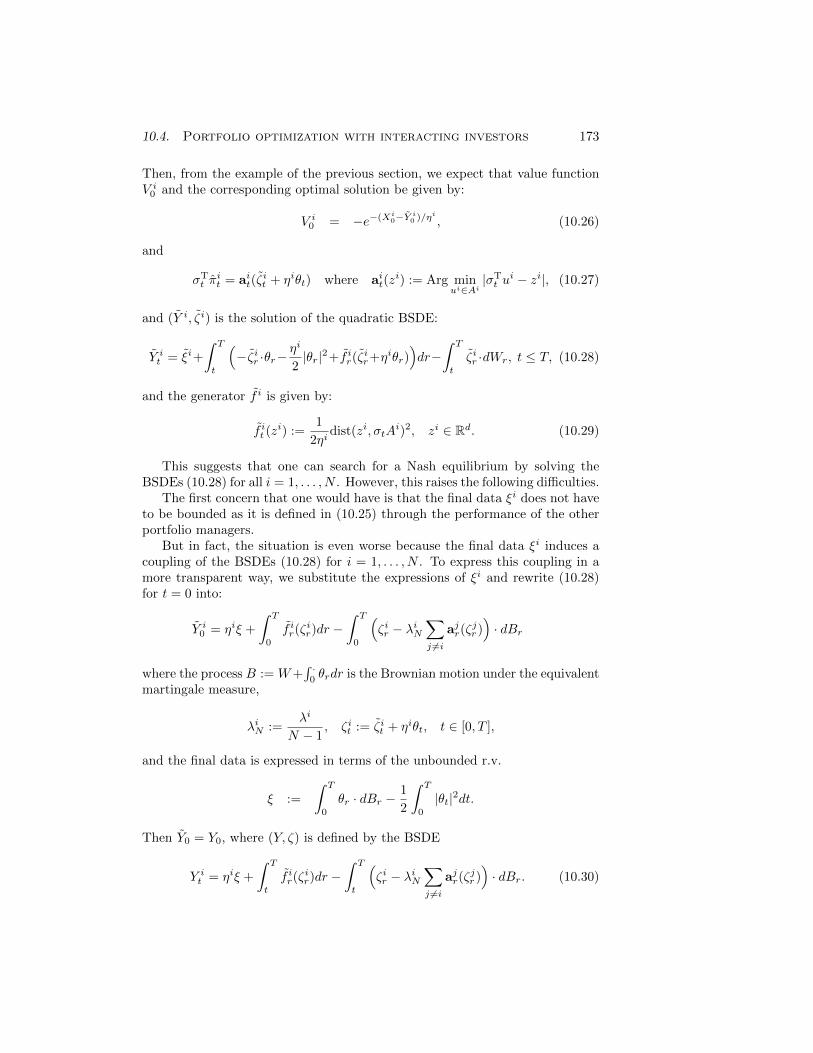
10.4. Portfolio optimization with interacting investors 173
Then, from the example of the previous section, we expect that value functionV i0 and the corresponding optimal solution be given by:
V i0 = −e−(Xi0−Yi0 )/ηi , (10.26)
and
σTt π
it = ait(ζ
it + ηiθt) where ait(z
i) := Arg minui∈Ai
|σTt u
i − zi|, (10.27)
and (Y i, ζi) is the solution of the quadratic BSDE:
Y it = ξi+
∫ T
t
(−ζir ·θr−
ηi
2|θr|2+f ir(ζ
ir+ηiθr)
)dr−
∫ T
t
ζir ·dWr, t ≤ T, (10.28)
and the generator f i is given by:
f it (zi) :=
1
2ηidist(zi, σtA
i)2, zi ∈ Rd. (10.29)
This suggests that one can search for a Nash equilibrium by solving theBSDEs (10.28) for all i = 1, . . . , N . However, this raises the following difficulties.
The first concern that one would have is that the final data ξi does not haveto be bounded as it is defined in (10.25) through the performance of the otherportfolio managers.
But in fact, the situation is even worse because the final data ξi induces acoupling of the BSDEs (10.28) for i = 1, . . . , N . To express this coupling in amore transparent way, we substitute the expressions of ξi and rewrite (10.28)for t = 0 into:
Y i0 = ηiξ +
∫ T
0
f ir(ζir)dr −
∫ T
0
(ζir − λiN
∑j 6=i
ajr(ζjr ))· dBr
where the process B := W+∫ .
0θrdr is the Brownian motion under the equivalent
martingale measure,
λiN :=λi
N − 1, ζit := ζit + ηiθt, t ∈ [0, T ],
and the final data is expressed in terms of the unbounded r.v.
ξ :=
∫ T
0
θr · dBr −1
2
∫ T
0
|θt|2dt.
Then Y0 = Y0, where (Y, ζ) is defined by the BSDE
Y it = ηiξ +
∫ T
t
f ir(ζir)dr −
∫ T
t
(ζir − λiN
∑j 6=i
ajr(ζjr ))· dBr. (10.30)

174 CHAPTER 10. QUADRATIC BSDEs
In order to sketch (10.30) into the BSDEs framework, we further introduce themapping φt : RNd −→ RNd defined by the components:
φit(ζ1, . . . , ζN ) := ζi − λiN
∑j 6=i
ajt (ζj) for all ζ1, . . . , ζN ∈ Rd. (10.31)
It turns out that the mapping φt is invertible under fairly general conditions.We shall prove this result in Lemma 10.18 below in the case where the Ai’s arelinear supspaces of Rd. Then one can rewrite (10.30) as:
Y it = ηiξ +
∫ T
t
f ir(Zr)dr −∫ T
t
Zir · dBr, (10.32)
where the generator f i is now given by:
f i(z) := f ir(φ−1
t (z)i)
for all z = (z1, . . . , zN ) ∈ RNd, (10.33)
and φ−1t (z)i indicates the i-th block component of size d of φ−1
t (z).
10.4.3 The case of linear constraints
We now focus on the case where the constraints sets are such that
Ai is a linear subspace of Rd, i = 1, . . . , N. (10.34)
Then, denoting by P it the orthogonal projection operator on σtAi (i.e. the image
of Ai by the matrix σt), we immediately compute that
ait(ζi) := P it (ζ
i) (10.35)
and
φit(ζ1, . . . , ζN ) := ζi − λiN
∑j 6=i
P jt (ζj), for i = 1, . . . , N. (10.36)
Lemma 10.18. Let (Ai)1≤i≤N be linear subspaces of Rd. Then, for all t ∈[0, T ]:(i) the linear mapping φt of (10.36) is invertible if and only if
N∏i=1
λi < 1 or
N⋂i=1
Ai = 0. (10.37)
(ii) this condition is equivalent to the invertibility of the matrices Id − Qit,i = 1, . . . , N , where
Qit :=∑j 6=i
λjN1 + λjN
P jt (Id + λjNPit ),

10.4. Portfolio optimization with interacting investors 175
(iii) under (10.37), the i−th component of φ−1t is given by:
φ−1t (z)i = (Id −Qit)−1
zi +∑j 6=i
1
1 + λjNP jt (λiNz
j − λjNzi)
.
Proof. We omit all t subscripts, and we denote µi := λiN . For arbitrary z1, . . . , zN
in Rd, we want to find a unique solution to the system
ζi − µi∑j 6=i
P jζj = zi, 1 ≤ i ≤ N. (10.38)
1. Since P j is a projection, we immediately compute that (Id + µjP j)−1 =
Id − µj
1+µj Pj . Substracting equations i and j from the above system, we see
that
µiP jζj = P j(Id + µjP j)−1(µj(Id + µiP i)ζi + µizj − µjzi
)=
1
1 + µjP j(µj(Id + µiP i)ζi + µizj − µjzi
).
Then it follows from (10.38) that
zi = ζi −∑j 6=i
1
1 + µjP j(µj(Id + µiP i)ζi + µizj − µjzi
),
and we can rewrite (10.38) equivalently as:Id −∑j 6=i
µj
1 + µjP j(Id + µiP i)
ζi = zi+∑j 6=i
1
1 + µjP j(µizj−µjzi), (10.39)
so that the invertibility of φ is now equivalent to the invertibility of the matricesId −Qi, i = 1, . . . , N , where Qi is introduced in statement of the lemma.2. We now prove that Id − Qi is invertible for every i = 1, . . . , N iff (10.37)holds true.
2a. First, assume to the contrary that λi = 1 for all i and ∩Ni=1Ai contains
a nonzero element x0. Then, it follows that y0 := σTx0 satisfies P iy0 = y0 forall i = 1, . . . , N , and therefore Qiy0 = y0. Hence Id −Qi is not invertible.
2b. Conversely, we consider separately two cases.
• If λi0 < 1 for some i0 ∈ 1, . . . , N, we estimate that
µi0
1 + µi0<
1N−1
1 + 1N−1
andµi
1 + µi≤
1N−1
1 + 1N−1
for i 6= i0.
Then for all i 6= i0 and x 6= 0, it follows that |Qix| < |x| proving thatI −Qi is invertible.

176 CHAPTER 10. QUADRATIC BSDEs
• If λi = 1 for all i = 1, . . . , N , then for all x ∈ Ker(Qi), we have x = Qixand therefore
|x| =∣∣∣∑j 6=i
µj
1 + µjP j(Id + µiP i)x
∣∣∣=
1
N
∣∣∣∑j 6=i
P j(Id +1
N − 1P i)x
∣∣∣≤ 1
N
∑j 6=i
(1 +1
N − 1|x| = |x|,
where we used the fact that the spectrum of the P i’s is reduced to 0, 1.Then equality holds in the above inequalities, which can only happen ifP ix = x for all i = 1, . . . , N . We can then conclude that ∩Ni=1Ker(Id −P i) = 0 implies that Id −Qi is invertible. This completes the proof as∩Ni=1Ker(Id − P i) = 0 is equivalent to ∩Ni=1A
i = 0.
♦
10.4.4 Nash equilibrium under deterministic coefficients
The discussion of Section 10.4.2 shows that the question of finding a Nash equi-librium for our problem reduces to the vector BSDE with quadratic generator(10.32), that we rewrite here for convenience:
Y it = ηiξ +
∫ T
t
f ir(Zr)dr −∫ T
t
Zir · dBr, (10.40)
where ξ :=∫ T
0θr · dBr − 1
2
∫ T0|θr|2dr, and the generator f i is given by:
f i(z) := f ir(φ−1
t (z)i)
for all z = (z1, . . . , zN ) ∈ RNd. (10.41)
Unfortunately, the problem of solving vector BSDEs with quadratic generator isstill not understood. Therefore, we will not continue in the generality assumedso far, and we will focus in the sequel on the case where
the Ai’s are vector subspaces of Rd, andσt = σ(t) and θt = θ(t) are deterministic functions.
(10.42)
Then, the vector BSDE reduces to:
Y it = ηiξ +1
2ηi
∫ T
t
∣∣∣(Id − P i(t))(φ(t)−1(Zr)i)∣∣∣2dr − ∫ T
t
Zir · dBr, (10.43)
where P it = P i(t) is deterministic, φ−1t (z)i = φ(t)−1(z)i is deterministic
and given explicitly by (10.18) (iii).

10.4. Portfolio optimization with interacting investors 177
In this case, an explicit solution of the vector BSDE is given by:
Zit = ηiθ(t)
Y it = −ηi
2
∫ T
0
|θ(t)|2dt+1
2ηi
∫ t
0
|(Id − P i(t))M i(t)θ(t)|2dt,(10.44)
where
M i(t) :=
Id −∑j 6=i
λjN1 + λjN
P j(t)(Id + λjNPi(t)
−1
×
ηiId +∑j 6=i
1
1 + λjNP j(t)(λiNη
j − λjNηi)
.
By (10.27), the candidate for Agent i−th optimal portfolio is also deterministicand given by:
πi := σ−1P iM iθ, i = 1, . . . , N. (10.45)
Proposition 10.19. In the context of the financial market with determinis-tic coefficients (10.42), the N−uple (π1, . . . , πN ) defined by (10.45) is a Nashequilibrium.
Proof. The above explicit solution of the vector BSDE induces an explicit solu-tion (Y i, ζi) of the coupled system of BSDEs (10.28), 1 ≤ i ≤ N with determin-istic ζi. In order to prove the required result, we have to argue by verificationfollowing the lines of the proof of Theorem 10.13 for every fixed i in 1, . . . , n.1. First for an arbitrary πi, we define the process
V πi
t := −e−(Xπi
t −Yit )/ηi , t ∈ [0, T ].
By Ito’s formula, it is immediately seen that this process is a local supermartin-gale (the generator has been defined precisely to satisfy this property !). By theadmissibility condition of Definition 10.16 together with the fact that Y i hasa gaussian distribution (as a diffusion process with deterministic coefficients),
it follows that the family V πiτ , τ ∈ T is uniformly bounded in L1+ε for any
ε > 0. Then the process V πi
is a supermartingale. By the arbitrariness ofπi ∈ Ai, this provides the first inequality
−e−(Xi0−Yi0 )/ηi ≥ V i0
((πj)j 6=i
).
2. We next prove that equality holds by verifying that πi ∈ Ai, and the pro-cess V π
i
is a martingale. This will provide the value function of Agent i’sportfolio optimization problem, and the fact that πi is optimal for the problemV i0((πj)j 6=i
).
That πi ∈ Ai is immediate; recall again that πi is deterministic. As inthe previous step, direct application of Ito’s formula shows that V π
i
is a local
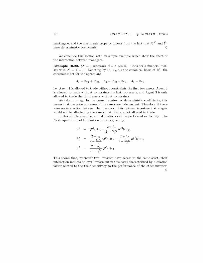
178 CHAPTER 10. QUADRATIC BSDEs
martingale, and the martingale property follows from the fact that X πi and Y i
have deterministic coefficients. ♦
We conclude this section with an simple example which show the effect ofthe interaction between managers.
Example 10.20. (N = 3 investors, d = 3 assets) Consider a financial mar-ket with N = d = 3. Denoting by (e1, e2, e3) the canonical basis of R3, theconstraints set for the agents are
A1 = Re1 + Re2, A2 = Re2 + Re3, A3 = Re3,
i.e. Agent 1 is allowed to trade without constraints the first two assets, Agent 2is allowed to trade without constraints the last two assets, and Agent 3 is onlyallowed to trade the third assets without constraints.
We take, σ = I3. In the present context of deterministic coefficients, thismeans that the price processes of the assets are independent. Therefore, if therewere no interaction between the investors, their optimal investment strategieswould not be affected by the assets that they are not allowed to trade.
In this simple example, all calculations can be performed explicitely. TheNash equilibrium of Propostion 10.19 is given by:
π1t = ηθ1(t)e1 +
2 + λ1
2− λ1λ2
2
ηθ2(t)e2,
π2t =
2 + λ2
2− λ1λ2
2
ηθ2(t)e2 +2 + λ2
2− λ2λ3
2
ηθ3(t)e3,
π3t =
2 + λ3
2− λ2λ3
2
ηθ3(t)e3.
This shows that, whenever two investors have access to the same asset, theirinteraction induces an over-investment in this asset characterized by a dilationfactor related to the their sensitivity to the performance of the other investor.
♦

Chapter 11
Probabilistic numericalmethods for nonlinearPDEs
In this chapter, we introduce a backward probabilistic scheme for the numericalapproximation of the solution of a nonlinear partial differential equation. Thescheme is decomposed into two steps:(i) The Monte Carlo step consists in isolating the linear generator of someunderlying diffusion process, so as to split the PDE into this linear part and aremaining nonlinear one.(ii) Evaluating the PDE along the underlying diffusion process, we obtain anatural discrete-time approximation by using finite differences approximationin the remaining nonlinear part of the equation.
Our main concern will be to prove the convergence of this discrete-timeapproximation. In particular, the above scheme involves the calculation of con-ditional expectations, that should be replaced by some approximation for anypractical implementation. The error analysis of this approximation will not beaddresses here.
Throughout this chapter, µ and σ are two functions from R+ × Rd to Rdand Sd, respectively. Let a := σ2, and define the linear operator:
LXϕ :=∂ϕ
∂t+ µ ·Dϕ+
1
2a ·D2ϕ.
Consider the map
F : (t, x, r, p, γ) ∈ R+ × Rd × R× Rd × Sd 7−→ F (x, r, p, γ) ∈ R,
which is assumed to be elliptic:
F (t, x, r, p, γ) ≥ F (t, x, r, p, γ′) for all γ ≥ γ′.
179

180 CHAPTER 11. NUMERICAL PROBABILITY FOR PDEs
Our main interest is on the numerical approximation for the Cauchy problem:
−LXv − F(·, v,Dv,D2v
)= 0, on [0, T )× Rd, (11.1)
v(T, ·) = g, on ∈ Rd. (11.2)
11.1 Discretization
LetW be an Rd-valued Brownian motion on a filtered probability space (Ω,F ,F,P).For a positive integer n, let h := T/n, ti = ih, i = 0, . . . , n, and consider the
one step ahead Euler discretization
Xt,xh := x+ µ(t, x)h+ σ(t, x)(Wt+h −Wt), (11.3)
of the diffusion X corresponding to the linear operator LX . Our analysis doesnot require any existence and uniqueness result for the underlying diffusion X.However, the subsequent formal discussion assumes it in order to provides anatural justification of our numerical scheme.
Assuming that the PDE (11.1) has a classical solution, it follows from Ito’sformula that
Eti,x[v(ti+1, Xti+1
)]= v (ti, x) + Eti,x
[∫ ti+1
ti
LXv(t,Xt)dt
]where we ignored the difficulties related to the local martingale part, and Eti,x :=E[·|Xti = x] denotes the expectation operator conditional on Xti = x. Sincev solves the PDE (11.1), this provides
v(ti, x) = Eti,x[v(ti+1, Xti+1
)]+ Eti,x
[∫ ti+1
ti
F (·, v,Dv,D2v)(t,Xt)dt
].
By approximating the Riemann integral, and replacing the process X by itsEuler discretization, this suggest the following approximation:
vh(T, .) := g and vh(ti, x) := Rti [vh(ti+1, .)](x), (11.4)
where we denoted for a function ψ : Rd −→ R with exponential growth:
Rt[ψ](x) := E[ψ(Xt,x
h )]
+ hF (t, ·,Dhψ) (x), (11.5)
with Dhψ :=(D0hψ,D1
hψ,D2hψ)T
, and:
Dkhψ(x) := E[Dkψ(Xt,xh )] for k = 0, 1, 2,
and Dk is the k−th order partial differential operator with respect to the spacevariable x. The differentiations in the above scheme are to be understood in thesense of distributions. This algorithm is well-defined whenever g has exponentialgrowth and F is a Lipschitz map. To see this, observe that any function with
181
exponential growth has weak gradient and Hessian, and the exponential growthis inherited at each time step from the Lipschitz property of F .
At this stage, the above backward algorithm presents the serious drawbackof involving the gradient Dvh(ti+1, .) and the Hessian D2vh(ti+1, .) in order tocompute vh(ti, .). The following result avoids this difficulty by an easy integra-tion by parts argument.
Lemma 11.1. Let f : Rd → R be a function with exponential growth. Then:
E[Dif(Xti,xh )] = E[f(Xti,x
h )Hhi (ti, x)] for i = 1, 2,
where
Hh1 =
1
hσ−1Wh and Hh
2 =1
h2σ−1
(WhW
Th − hId
)σ−1. (11.6)
Proof. We only provide the argument in the one-dimensional case; the extensionto any dimension d is immediate. Let G be a one dimensional Gaussian randomvariable with men m and variance v. Then, for any function f with exponentialgrowth, it follows from an integration by parts that:
E[f ′(G)] =
∫f ′(s)e−
12
(s−m)2
vds√2πv
=
∫f(s)
s−mv
e−12
(s−m)2
vds√2πv
= E[f(G)
G−mv
],
where the remaining term in the integration by parts formula vanishes by theexponential growth of f . This implies the required result for i = 1.
To obtain the result for i = 2, we continue by integrating by parts oncemore:
E[f ′′(G)] = E[f ′(G)
G−mv
]=
∫f ′(s)
s−mv
e−12
(s−m)2
vds√2πv
=
∫f(s)
(−1
v+ (
s−mv
)2
)e−
12
(s−m)2
vds√2πv
= E[f(G)
(G−m)2 − vv2
].
♦
In the sequel, we shall denote Hh := (1, Hh1 , H
h2 )T. In view of the last lemma,
we may rewrite the discretization scheme (11.4) into:
vh(T, .) = g and vh(ti, x) = Rti
[vh(ti+1, .)
](x), (11.7)
where
Rti [ψ](x) = E[ψ(Xt,x
h )]
+ hF (t, ·,Dhψ) (x),
182 CHAPTER 11. NUMERICAL PROBABILITY FOR PDEs
and
Dkhψ(x) := E[ψ(Xt,x
h )Hkh(t, x)
]for k = 0, 1, 2. (11.8)
Observe that the choice of the drift and the diffusion coefficients µ and σ inthe nonlinear PDE (11.1) is arbitrary. So far, it has been only used in order todefine the underlying diffusion X. Our convergence result will however placesome restrictions on the choice of the diffusion coefficient, see Remark 11.6.
Once the linear operator LX is chosen in the nonlinear PDE, the abovealgorithm handles the remaining nonlinearity by the classical finite differencesapproximation. This connection with finite differences is motivated by the fol-lowing formal interpretation of Lemma 11.1, where for ease of presentation, weset d = 1, µ ≡ 0, and σ(x) ≡ 1:
• Consider the binomial random walk approximation of the Brownian mo-tion Wtk :=
∑kj=1 wj , tk := kh, k ≥ 1, where wj , j ≥ 1 are independent
random variables distributed as 12
(δ√h + δ−
√h
). Then, this induces
the following approximation:
D1hψ(x) := E
[ψ(Xt,x
h )Hh1
]≈ ψ(x+
√h)− ψ(x−
√h)
2√h
,
which is the centered finite differences approximation of the gradient.
• Similarly, consider the trinomial random walk approximation Wtk :=∑kj=1 wj , tk := kh, k ≥ 1, where wj , j ≥ 1 are independent random
variables distributed as 16
(δ√
3h + 4δ0 + δ−√
3h
), so that E[wnj ] =
E[Wnh ] for all integers n ≤ 4. Then, this induces the following approxima-
tion:
D2hψ(x) := E
[ψ(Xt,x
h )Hh2
]≈ ψ(x+
√3h)− 2ψ(x) + ψ(x−
√3h)
3h,
which is the centered finite differences approximation of the Hessian.
In view of the above interpretation, the numerical scheme (11.7) can be viewedas a mixed Monte Carlo–Finite Differences algorithm. The Monte Carlo compo-nent of the scheme consists in the choice of an underlying diffusion process X.The finite differences component of the scheme consists in approximating theremaining nonlinearity by means of the integration-by-parts formula of Lemma11.1.
11.2 Convergence of the discrete-time approxi-mation
The main convergence result of this section requires the following assumptions.

183
Assumption 11.2. The PDE (11.1) has comparison for bounded functions, i.e.for any bounded upper semicontinuous viscosity subsolution u and any boundedlower semicontinuous viscosity supersolution v on [0, T )× Rd, satisfying
u(T, ·) ≤ v(T, ·),
we have u ≤ v.
For our next assumption, we denote by Fr, Fp and Fγ the partial gradientsof F with respect to r, p and γ, respectively. We also denote by F−γ the pseudo-inverse of the non-negative symmetric matrix Fγ . We recall that any Lipschitzfunction is differentiable a.e.
Assumption 11.3. (i) The nonlinearity F is Lipschitz-continuous with re-spect to (x, r, p, γ) uniformly in t, and |F (·, ·, 0, 0, 0)|∞ <∞.(ii) F is elliptic and dominated by the diffusion of the linear operator LX , i.e.
Fγ ≤ a on Rd × R× Rd × Sd. (11.9)
(iii) Fp ∈ Image(Fγ) and∣∣FTp F−γ Fp
∣∣∞ < +∞.
Before commenting this assumption, we state our main convergence result.
Theorem 11.4. Let Assumptions 11.2 and 11.3 hold true, and assume that µ, σare Lipschitz-continuous and σ is invertible. Then for every bounded Lipschitzfunction g, there exists a bounded function v so that
vh −→ v locally uniformly.
In addition, v is the unique bounded viscosity solution of problem (11.1)-(11.2).
The proof of this result is reported in the subsection 11.4. We conclude bysome remarks.
Remark 11.5. Assumption 11.3 (iii) is equivalent to
|m−F |∞ <∞ where mF := minw∈Rd
Fp · w + wTFγw
. (11.10)
To see this observe first that Fγ is a symmetric matrix, as a consequence ofthe ellipticity of F . Then, any w ∈ Rd has an orthogonal decomposition w =w1 + w2 ∈ Ker(Fγ)⊕ Image(Fγ), and by the nonnegativity of Fγ :
Fp · w + wTFγw = Fp · w1 + Fp · w2 + wT2 Fγw2
= −1
4FTp F−γ Fp + Fp · w1 +
∣∣12
(F−γ )1/2 · Fp − F 1/2γ w2
∣∣2.Remark 11.6. Assumption 11.3 (ii) places some restrictions on the choice ofthe linear operator LX in the nonlinear PDE (11.1). First, F is required tobe uniformly elliptic, implying an upper bound on the choice of the diffusionmatrix σ. Since σ2 ∈ S+
d , this implies in particular that our main results do notapply to general degenerate nonlinear parabolic PDEs. Second, the diffusion ofthe linear operator σ is required to dominate the nonlinearity F which placesimplicitly a lower bound on the choice of the diffusion σ.

184 CHAPTER 11. NUMERICAL PROBABILITY FOR PDEs
Example 11.7. Let us consider the nonlinear PDE in the one-dimensionalcase −∂v∂t −
12
(a2v+
xx − b2v−xx)
where 0 < b < a are given constants. Then if werestrict the choice of the diffusion to be constant, it follows from Assumption11.3 that 1
3a2 ≤ σ2 ≤ b2, which implies that a2 ≤ 3b2. If the parameters a and
b do not satisfy the latter condition, then the diffusion σ has to be chosen to bestate and time dependent.
Remark 11.8. Under the boundedness condition on the coefficients µ andσ, the restriction to a bounded terminal data g in the above Theorem 11.4can be relaxed by an immediate change of variable. Let g be a function withα−exponential growth for some α > 0. Fix some M > 0, and let ρ be anarbitrary smooth positive function with:
ρ(x) = eα|x| for |x| ≥M,
so that both ρ(x)−1∇ρ(x) and ρ(x)−1∇2ρ(x) are bounded. Let
u(t, x) := ρ(x)−1v(t, x) for (t, x) ∈ [0, T ]× Rd.
Then, the nonlinear PDE problem (11.1)-(11.2) satisfied by v converts into thefollowing nonlinear PDE for u:
−LXu− F(·, u,Du,D2u
)= 0 on [0, T )× Rd (11.11)
v(T, ·) = g := ρ−1g on Rd,
where
F (t, x, r, p, γ) := rµ(x) · ρ−1∇ρ+1
2Tr[a(x)
(rρ−1∇2ρ+ 2pρ−1∇ρT
)]+ρ−1F
(t, x, rρ, r∇ρ+ pρ, r∇2ρ+ 2p∇ρT + ργ
).
Recall that the coefficients µ and σ are assumed to be bounded. Then, it iseasy to see that F satisfies the same conditions as F . Since g is bounded, theconvergence Theorem 11.4 applies to the nonlinear PDE (11.11). ♦
11.3 Consistency, monotonicity and stability
The proof of Theorem 11.4 is based on the monotone schemes method of Barlesand Souganidis [5] which exploits the stability properties of viscosity solutions.The monotone schemes method requires three conditions: consistency, mono-tonicity and stability that we now state in the context of backward scheme(11.7).
To emphasize on the dependence on the small parameter h in this section,we will use the notation:
Th[ϕ](t, x) := Rt[ϕ(t+ h, .)](x) for all ϕ : R+ × Rd −→ R.

185
Lemma 11.9 (Consistency). Let ϕ be a smooth function with bounded deriva-tives. Then for all (t, x) ∈ [0, T ]× Rd:
lim(t′, x′) → (t, x)(h, c) → (0, 0)
t′ + h ≤ T
([c+ ϕ]−Th[c+ ϕ]
)(t′, x′)
h= −
(LXϕ+ F (·, ϕ,Dϕ,D2ϕ)
)(t, x).
The proof is a straightforward application of Ito’s formula, and is omitted.
Lemma 11.10 (Monotonicity). Let ϕ,ψ : [0, T ] × Rd −→ R be two Lipschitzfunctions with ϕ ≤ ψ. Then:
Th[ϕ](t, x) ≤ Th[ψ](t, x) + Ch E[(ψ − ϕ)(t+ h, Xt,xh )] for some C > 0
depending only on the constant mF in (11.10).
Proof. By Lemma 11.1 the operator Th can be written as:
Th[ψ](t, x) = E[ψ(Xt,x
h )]
+ hF(t, x,E[ψ(Xt,x
h )Hh(t, x)]).
Let f := ψ − ϕ ≥ 0 where ϕ and ψ are as in the statement of the lemma. LetFτ denote the partial gradient with respect to τ = (r, p, γ). By the mean valueTheorem:
Th[ψ](t, x)−Th[ϕ](t, x) = E[f(Xt,x
h )]
+ hFτ (θ) · Dhf(Xt,xh )
= E[f(Xt,x
h ) (1 + hFτ (θ) ·Hh(t, x))],
for some θ = (t, x, r, p, γ). By the definition of Hh(t, x):
Th[ψ]−Th[ϕ]
= E[f(Xt,x
h )(1 + hFr + Fp.σ
−1Wh + h−1Fγ · σ−1(WhWTh − hI)σ−1
)],
where the dependence on θ and x has been omitted for notational simplicity.Since Fγ ≤ a by Assumption 11.3, we have 1− a−1 · Fγ ≥ 0 and therefore:
Th[ψ]−Th[ϕ] ≥ E[f(Xt,x
h )(hFr + Fp.σ
−1Wh + h−1Fγ · σ−1WhWTh σ−1)]
= E[f(Xt,x
h )
(hFr + hFp.σ
−1Wh
h+ hFγ · σ−1WhW
Th
h2σ−1
)].
Recall the function mF defined in (11.10). Under Assumption 11.3, it followsfrom Remark 11.5 that K := |m−F |∞ <∞. Then
Fp.σ−1Wh
h+ hFγ · σ−1WhW
Th
h2σ−1 ≥ −K,
and therefore:
Th[ψ]−Th[ϕ] ≥ E[f(Xt,x
h ) (hFr − hK)]≥ −C ′hE
[f(Xt,x
h )]
for some constant C > 0, where the last inequality follows from (11.10). ♦

186 CHAPTER 11. NUMERICAL PROBABILITY FOR PDEs
Lemma 11.11 (Stability). Let ϕ,ψ : [0, T ] × Rd −→ R be two L∞−boundedfunctions. Then there exists a constant C > 0 such that∣∣Th[ϕ]−Th[ψ]
∣∣∞ ≤ |ϕ− ψ|∞(1 + Ch).
In particular, if g is L∞−bounded, then the family (vh)h defined in (11.7) isL∞−bounded, uniformly in h.
Proof. Let f := ϕ− ψ. Arguing as in the previous proof, we see that:
Th[ϕ]−Th[ψ] = E[f(Xh)
(1− a−1 · Fγ + h|Ah|2 + hFr −
h
4FTp F−γ Fp
)].
where
Ah =1
2(F−γ )1/2Fp − F 1/2
γ σ−1Wh
h.
Since 1 − Tr[a−1Fγ ] ≥ 0, |Fr|∞ < ∞, and |FTp F−γ Fp|∞ < ∞ by Assumption
11.3, it follows that
|Th[ϕ]−Th[ψ]|∞ ≤ |f |∞(1− a−1 · Fγ + hE[|Ah|2] + Ch
)But, E[|Ah|2] = h
4FTp F−γ Fp + a−1 ·Fγ . Therefore, using again Assumption 11.3,
we see that:
|Th[ϕ]−Th[ψ]|∞ ≤ |f |∞(
1 +h
4FTp F−γ Fp + Ch
)≤ |f |∞(1 + Ch).
To prove that the family (vh)h is bounded, we proceed by backward induction.By the assumption of the lemma vh(T, .) = g is L∞−bounded. We next fixsome i < n and we assume that |vh(tj , .)|∞ ≤ Cj for every i + 1 ≤ j ≤ n − 1.Proceeding as in the proof of Lemma 11.10 with ϕ ≡ vh(ti+1, .) and ψ ≡ 0, wesee that ∣∣vh(ti, .)
∣∣∞ ≤ h |F (t, x, 0, 0, 0)|+ Ci+1(1 + Ch).
Since F (t, x, 0, 0, 0) is bounded by Assumption 11.3, it follows from the discreteGronwall inequality that |vh(ti, .)|∞ ≤ CeCT for some constant C independentof h. ♦
11.4 The Barles-Souganidis monotone scheme
This section is dedicated to the proof of Theorem 11.4. We emphasize on the factthat the subsequent argument applies to any numerical scheme which satisfiesthe consistency, monotonicity and stability properties. In the present situation,we also need to prove a technical result concerning the limiting behavior of theboundary condition at T . This will be needed in order to use the comparison
187
result which is assumed to hold for the equation. The statement and its proofare collected in Lemma 11.12.
Proof of Theorem 11.4 1. By the stability property of Lemma 11.11, itfollows that the relaxed semicontinious envelopes
v(t, x) := lim inf(h,t′,x′)→(0,t,x)
vh(t′, x′) and v(t, x) := lim sup(h,t′,x′)→(0,t,x)
vh(t′, x′)
are bounded. We shall prove in Step 2 below that v and v are viscosity superso-lution and subsolution, respectively. The final ingredient is reported in Lemma11.12 below which states that v(T, .) = v(T, .). Then, the proof is completed byappealing to the comparison property of Assumption 11.2.2. We only prove that v is a viscosity supersolution of (11.1). The proof of theviscosity subsolution property of v follows exactly the same line of argument.Let (t0, x0) ∈ [0, T )× Rd and ϕ ∈ C2
([0, T ]× Rd
)be such that
0 = (v − ϕ)(t0, x0) = (strict) min[0,T ]×Rd
(v − ϕ). (11.12)
Since vh is uniformly bounded in h, we may assume without loss of generalitythat ϕ is bounded. Let (hn, tn, xn)n be a sequence such that
hn → 0, (tn, xn)→ (t0, x0), and vhn(tn, xn) −→ v(t0, x0). (11.13)
For a positive scalar r with 2r < T − t0, we denote by Br(tn, xn) the ball ofradius r centered at (tn, xn), and we introduce:
δn := (vhn∗ − ϕ)(tn, xn) = minBr(tn,xn)
(vhn∗ − ϕ), (11.14)
where vhn∗ is the lower-semicontinuous envelope of vhn . We claim that
δn −→ 0 and (tn, xn) −→ (t0, x0). (11.15)
This claim is proved in Step 3 below. By the definition of vhn∗ , we may find asequence (t′n, x
′n)n≥1 converging to (t0, x0), such that:
|vhn(t′n, x′n)− vhn∗ (tn, xn)| ≤ h2
n and |ϕ(t′n, x′n)− ϕ(tn, xn)| ≤ h2
n. (11.16)
By (11.14), (11.16), and the definition of the functions vh in (11.7), we have
2h2n + δn + ϕ(t′n, x
′n) ≥ h2
n + δn + ϕ(tn, xn)
= h2n + vhn∗ (tn, xn)
≥ vhn(t′n, x′n)
= Thn [vhn ](t′n, x′n)
≥ Thn [ϕhn + δn](t′n, x′n)
+ChnE[(vhn − ϕ− δn)
(Xt′n,x
′n
hn
)],

188 CHAPTER 11. NUMERICAL PROBABILITY FOR PDEs
where the last inequality follows from (11.14) and the monotonicity property ofLemma 11.10. Dividing by hn, the extremes of this inequality provide:
δn + ϕ(t′n, x′n)−Thn [ϕhn + δn](t′n, x
′n)
hn≥ CE
[(uhn − ϕ− δn)
(Xt′n,x
′n
hn
)].
We now send n to infinity. The right hand-side converges to zero by (11.13),(11.15), and the dominated convergence theorem. For the left hand-side term,we use the consistency result of Lemma 11.9. This leads to(
− LXϕ− F (., ϕ,Dϕ,D2ϕ))(t0, x0) ≥ 0,
as required.3. We now prove Claim (11.15). Since (tn, xn)n is a bounded sequence, we mayextract a subsequence, still named (tn, xn)n, converging to some (t, x). Then:
0 = (v − ϕ)(t0, x0)
= limn→∞
(vhn − ϕ)(tn, xn)
≥ lim supn→∞
(vhn∗ − ϕ)(tn, xn)
≥ lim supn→∞
(vhn∗ − ϕ)(tn, xn)
≥ lim infn→∞
(vhn∗ − ϕ)(tn, xn)
≥ (v − ϕ)(t, x).
Since (t0, x0) is a strict minimizer of the difference (v−ϕ), this implies (11.15).♦
The following result is needed in order to use the comparison property ofAssumption 11.2. We shall not report its long technical proof, see [19].
Lemma 11.12. The function vh is Lipschtiz in x, 1/2−Holder continuous int, uniformly in h, and for all x ∈ Rd, we have
|vh(t, x)− g(x)| ≤ C(T − t) 12 .

Chapter 12
Introduction to Finitedifferences methods
by Agnes Tourin,Fields Institute, Immersion Fellowship
In this lecture, I discuss the practical aspects of designing Finite Differencemethods for Hamilton-Jacobi-Bellman equations of parabolic type arising inQuantitative Finance. The approach is based on the very powerful and simpleframework developed by Barles-Souganidis [5], see the review of the previouschapter. The key property here is the monotonicity which guarantees that thescheme satisfies the same ellipticity condition as the HJB operator. I will providea number of examples of monotone schemes in these notes. In practice, pureFinite Difference schemes are only useful in 1,2 or at most 3 spatial dimensions.One of their merits is to be quite simple and easy to implement. Also, as shownin the previous chapter, they can also be combined with Monte Carlo methodsto solve nonlinear parabolic PDEs.
Such approximations are now fairly standard and you will find many inter-esting examples available in the literature. For instance, I suggest the articles onthe subject by P. Forsyth (see [41], [34], [43]). There is also a classical book writ-ten by H. J. Kushner and Paul Dupuis [29] on numerical methods for stochasticcontrol problems. Finally, for a basic introduction to Finite Difference methodsfor linear parabolic PDEs, I recommend the book by J.W. Thomas [40].
189

190 CHAPTER 12. INTRODUCTION TO FINITE DIFFERENCES
12.1 Overview of the Barles-Souganidis frame-work
Consider the parabolic PDE
ut − F (t, x, u,Du,D2u) = 0 in (0, T ]× RN (12.1)
u(0, x) = u0(x) in RN (12.2)
where F is elliptic
F (t, x, u, p, A) ≥ F (t, x, u, p,B), if A ≥ B.
For the sake of simplicity, we assume that u0 is bounded in RN .The main application we have in mind is, for instance, to an operator F
coming from a stochastic control problem:
F (t, x, r, p,X) = supα∈A−Tr[aα(t, x)X]− bα(t, x)p− cα(t, x)r − fα(t, x)
where aα = 12σ
ασαT .Typically, the set of control A is compact or finite, all the coefficients in the
equations are bounded and Lipschitz continuous in x, Holder with coefficient 12
in t and all the bounds are independent of α. Then the unique viscosity solutionu of (12.1) is a bounded and Lipschitz continuous function and is the solution ofthe underlying stochastic control problem. The ideas, concepts and techniquesactually apply to a broader range of optimal control problems. In particular,you can adapt the techniques to handle different situations, even possibly treatsome delicate singular control problems.
In the previous chapter, our convergence result required the technical lemma11.12 in order for the comparison result to apply. However, an easier statementof the Barles-Souganidis method can be obtained at the price of assuming astronger comparison result in the following sense.
Definition 12.1. We say that the problem (12.1)-(12.2) satisfies the strongcomparison principle for bounded solution if for all bounded functions u ∈ USCand v ∈ LSC such that:
• u (resp. v) is a viscosity subsolution (resp. supersolution) of (12.1) on(0, T ]× RN ,
• the boundary condition holds in the viscosity sense
maxut − F (., u,Du,D2u), u− u0 ≥ 0 on 0 × RN
minut − F (., u,Du,D2u), u− u0 ≤ 0 on 0 × RN ,
we have u ≤ v on [0, T ]× RN .

12.1. Overview of monotonic schemes 191
Under the strong comparison principle, any monotonic stable and consistentscheme ahieves convergence, and there is no need to analyze the behavior of thescheme near the boundary.
The aim is to build an approximation scheme which preserves the ellipticity.This discrete ellipticity property is called monotonicity. The monotonicity,together with the consistency of the scheme and some regularity ensure itsconvergence to the unique viscosity solution of the PDE (12.1),(12.2). It isworth insisting on the fact that if the scheme is not monotone, it may failto converge to the correct solution (see [34] for an example)! We present thetheory rather informally and we refer to the original articles for more details.The general concepts and machinery apply to a wide range of equations but thereader needs to be aware that each PDE has its own peculiarities and that, inpractice, the techniques must be tailored to each particular application.
A numerical scheme is an equation of the following form
S(h, t, x, uh(t, x), [uh]t,x) = 0 for (t, x) in Gh\t = 0 (12.3)
uh(0, x) = u0(x) in Gh ∩ t = 0 (12.4)
where h = (∆t,∆x) , Gh = ∆t0, 1, ..., nT ×∆xZN is the grid, uh standsfor the approximation of u on the grid, uh(t, x) is the approximation uh at thepoint (t, x) and [uh]t,x represents the value of uh at other points than (t, x).Note that uh can be both interpreted as a function defined at the grid pointsonly or on the whole space. Indeed if one knows the value of uh on the mesh, acontinuous version of uh can be constructed by linear interpolation.
The first and crucial condition in the Barles-Souganidis framework is:
Monotonicity S(h, t, x, r, u) ≥ S(h, t, x, r, v) whenever u ≤ v.
The monotonicity assumption can be weakened. This was indeed the casein the previous chapter. We only need it to hold approximately, with a marginof error that vanishes to 0 as h goes to 0.
Consistency For every smooth function φ(t, x):
limh→0,(n∆t,i∆x)→(t,x),c→0
S(h, n∆t, i∆x,Φ(t, x) + c, [Φ(t, x) + c]t,x) =
Φt + F (t, x,Φ(t, x), DΦ, D2Φ).
The final condition is:
Stability For every h > 0, the scheme has a solution uh which is uniformlybounded independently of h.
Theorem 12.2. Assume that the problem (12.1)-(12.2) satisfies the strongcomparison principle for bounded functions. Assume further that the scheme

192 CHAPTER 12. INTRODUCTION TO FINITE DIFFERENCES
(12.3),(12.4) satisfies the consistency, monotonicity and stability properties.Then, its solution uh converges locally uniformly to the unique viscosity solutionof (12.1),(12.2).
12.2 First examples
12.2.1 The heat equation: the classic explicit and implicitschemes
First, let me recall the classic explicit and implicit schemes for the heat equation:
ut − uxx = 0 in (0, T ]× R. (12.5)
u(0, x) = u0(x) (12.6)
and verify that these schemes satisfy the required properties. It is well-knownthat the analysis of the linear heat equation does not require the machinery ofviscosity solutions. Our intention here is to understand the connection betweenthe theory for linear parabolic equations and the theory of viscosity solutions.More precisely, our goal is to verify that the standard finite difference approxi-mations for the heat equation are convergent in the Barles-Souganidis sense.
The standard explicit scheme:
un+1i − uni
∆t=uni+1 + uni−1 − 2uni
∆X2.
Since this scheme is explicit, it is very easy to compute at each time step n+ 1the value of the approximation (un+1
i )i from the value of the approximation atthe time step n, namely (uni )i.
un+1i = uni + ∆t
(uni+1 + uni−1 − 2uni
∆X2
).
Note that we may define the scheme S by setting:
S(∆t,∆x, (n+ 1)∆T, i∆x, un+1i , [uni−1, u
ni , u
ni+1]) =
un+1i − uni
∆t−uni+1 + uni−1 − 2uni
∆X2.
Let us now discuss the properties of this scheme. Clearly, it is consistent withthe equation since formally, the truncation error is of order two in space andorder one in time. Let us recall how one can calculate the truncation error fora smooth function u with bounded partial derivatives. Simply write the taylorexpansions
uni+1 = uni + ux(n∆t, xi)∆X +1
2uxx(n∆t, xi)∆X
2 + uxxx1
6∆X3+

12.2. First examples 193
1
24uxxxx∆X4 + ∆X4ε(∆X)
and
uni−1 = uni − ux(n∆t, xi)∆X +1
2uxx(n∆t, xi)∆X
2 − 1
6uxxx∆X3+
1
24uxxxx∆X4 + ∆X4ε(∆X)
Then, adding up the two expansions, subtracting 2uni from the left- and righthand sides and dividing by ∆X2, one obtains
uni+1 + uni−1 − 2uni∆X2
= uxx +1
12uxxxx∆X2 + o(∆X2)
and thus the truncation error for this approximation of the second spatial deriva-tive is of order 2. Similarly the expansion
un+1i = uni + ut(n∆t, xi)∆t+
1
2utt(n∆t, xi)∆t
2 + ∆t2ε(∆t)
yieldsun+1i − uni
∆t= ut(n∆t, xi) +
1
2utt∆t+ ∆tε(∆t).
The truncation error for the approximation of the first derivative in time is oforder 1 only (for more details about computation of truncations errors, see thebook by Thomas [40]).Furthermore, the approximation S is monotone if and only if S is decreasingin uni , u
ni+1 and uni−1. First of all, it is unconditionally decreasing with respect
to both uni−1 and uni+1. Secondly, it is only decreasing in uni if the following CFLcondition is satisfied:
−1 + 2∆t
∆X2≤ 0
or equivalently
∆t ≤ 1
2∆X2.
The standard implicit schemeFor many financial applications, the explicit scheme turns out to be very
inaccurate because the CFL condition forces the time step to be so small thatthe rounding error dominates the total computational error (computational er-ror=rounding error+truncation error). Most of the time, an implicit scheme ispreferred because it is unconditionally convergent, regardless of the size of thetime step. We now evaluate the second derivative at time (n+ 1)∆t instead oftime n∆t,
un+1i − uni
∆t=un+1i+1 + un+1
i−1 − 2un+1i
∆X2.

194 CHAPTER 12. INTRODUCTION TO FINITE DIFFERENCES
Implementing an algorithm allowing to compute the approximation is less obvi-ous here. This discrete equation may be converted into a linear system of equa-tions and the algorithm will then consist in inverting a tridiagonal matrix. Thetruncation errors for smooth functions are the same as for the explicit schemeand the consistency follows from this analysis.
We claim that for any choice of the time step, the implicit scheme is mono-tone. In order to verify that claim, let us rewrite the implicit scheme using thenotation S:
S(∆t,∆x, (n+ 1)∆T, i∆x, un+1i , [un+1
i−1 , uni , u
n+1i+1 ]) =
un+1i − uni
∆t−un+1i+1 + un+1
i−1 − 2un+1i
∆X2.
Since S is decreasing in uni , un+1i+1 and un+1
i−1 the implicit scheme is uncondition-ally monotone.
12.2.2 The Black-Scholes-Merton PDE
The price of a European call u(t, x) satisfies the degenerate linear PDE
ut + ru− 1
2σ2x2uxx − rxux = 0 in (0, T ]× (0,+∞)
u(0, x) = (x−K)+.
The Black-Scholes-Merton PDE is linear and its elliptic operator is degenerate.The first derivative ux can be easily approximated in a monotone way using aforward Finite Difference
−rxux ≈ −rxiun+1i+1 − u
n+1i
∆x.
One can, for instance, implement the implicit scheme
S(∆t,∆x, (n+ 1)∆T, i∆x, un+1i , [un+1
i−1 , uni , u
n+1i+1 ]) =
un+1i − uni
∆t+ run+1
i − 1
2(i∆x)2u
n+1i+1 + un+1
i−1 − 2un+1i
∆X2−
ri∆xun+1i+1 − u
n+1i
∆x.
12.3 A nonlinear example: The Passport Op-tion
12.3.1 Problem formulation
It is an interesting example of a one-dimensional nonlinear HJB equation. Ipresent only briefly the underlying model here and refer to the article [41] for

12.3. A nonlinear example 195
more details and references. A passport option is an option on the balance of atrading account. The holder can trade an underlying asset S over a finite timehorizon [0, T ]. At maturity, the holder keeps any net gain, while the writer bearsany loss. The number of shares q of Stock held is bounded by a given numberC. Without any loss of generality, this number is commonly assumed to be 1(the problem can be solved in full generality by using the appropriate scaling).The Stock S follows a Geometric Brownian motion with drift µ and volatility σ,r is the risk free interest rate, γ is the dividend rate, rt is the interest rate forthe trading account and rc is its cost of carry rate. The option price V (t, S,W ),which depends on S and on the accumulated wealth W in the trading accountsolves the PDE
−Vt + rV − (r −γ)SVS − sup|q|≤1
−((γ − r + rc)qS − rtW )VW +1
2σ2S2(VSS + 2qVSW + q2VWW ) = 0
V (T, S,W ) = max(W, 0)
Next, one can reduce this problem to a one dimensional equation by intro-ducing the variable x = W/S and the new function u satisfyingV (T − t, S,W ) = Su(t, x). The PDE for u then reads
ut +γu− sup|q|≤1
((r −γ −rc)q −(r −γ −rt)x)ux +1
2σ2(x−q)2uxx
u(0, x) = max(x, 0).
Note that, in this example, the solution is no longer bounded but grows at mostlinearly at infinity. The Barles-Souganidis [5] framework can be slightly modifiedto accommodate the linear growth of the value function at infinity.
When the payoff is convex, it is easy to see that the optimal value for q iseither +1 or −1. When the payoff is no longer convex, the supremum may be
achieved inside the interval at q∗ = x− (r−γ−rc)uxσ2uxx
. For simplicity, we consideronly the convex case.
12.3.2 Finite Difference approximation
To simplify further , we focus on a simple case: we assume that r − γ − rt = 0and r − γ − rc < 0. This equation is still fairly difficult to solve because theapproximation scheme must depend on the control q.
ut +γu−max(r −γ −rc)ux +1
2σ2(x−1)2uxx,
−(r −γ −rc)ux +1
2σ2(x+1)2uxx
u(0, x) = max(x, 0)

196 CHAPTER 12. INTRODUCTION TO FINITE DIFFERENCES
One can easily construct an explicit monotone scheme by using the appropri-ate forward or backward finite difference for the first partial derivative. Often,this type of scheme is called ”upwind” because you move along the directionprescribed by the deterministic dynamics b(x, α∗) corresponding to the optimalcontrol α∗ and pick the corresponding neighbor. For instance, for the passportoption, the dynamics are
For q∗ = 1, bα∗(t, x) = q∗(r − γ − rc) = (r − γ − rc) < 0
For q∗ = −1, bα∗(t, x) = −(r − γ − rc) > 0
and the corresponding upwind Finite Differences are
For q∗ = 1, ux ≈ D−uniFor q∗ = −1, ux ≈ D+uni
where we used the standard notations
D−uni =uni − uni−1
∆x,D+uni =
uni+1 − uni∆x
.
Then the scheme reads
un+1i − uni
∆t+ γuni −max
(r −γ −rc)uni − uni−1
∆x+
1
2σ2(xi−1)2u
ni+1 + uni−1 − 2uni
∆x2,
−(r −γ −rc)uni+1 − uni
∆x+
1
2σ2(xi+1)2u
ni+1 + uni−1 − 2uni
∆x2 = 0.
This scheme clearly satisfies the monotonicity assumption under the CFLcondition
∆t ≤ 1
γ + |r−γ−rc|∆x + σ2 maxmaxii∆x−12,maxii∆x+12
∆x2
.
Approximating the first spatial derivative by the classic centered finite dif-
ference, i.e. ux ≈uni+1−u
ni−1
2∆x would not yield a monotone scheme here.
Note that this condition is very restrictive. First of all, as expected, ∆t has tobe of order ∆x2. Furthermore, ∆t also depends on the size of the grid through theterms (i∆x−1)2, (i∆x−1)2 and even approaches 0 as the size of the domain goesto infinity. In this situation, we renounce using the above explicit scheme andreplace it by the fully implicit upwind scheme which is unconditionally monotone.

12.4. The Bannans-Zidani approximation 197
un+1i − uni
∆t+ γun+1
i −max
(r −γ −rc)un+1i − un+1
i−1
∆x+
1
2σ2(xi−1)2u
n+1i+1 + un+1
i−1 − 2un+1i
∆x2,
−(r −γ −rc)un+1i+1 − u
n+1i
∆x+
1
2σ2(xi+1)2u
n+1i+1 + un+1
i−1 − 2un+1i
∆x2 = 0.
Inverting the above scheme is challenging because it depends on the control.This can be done using the classic iterative Howard algorithm which we describebelow in a general setting. However, it may be time-consuming to compute thesolution of a nonlinear Finite Difference scheme, i.e invert an implicit schemeusing an iterative method.
12.3.3 Howard algorithm
We denote by unh, un+1h the approximations at time n and n+1. We can rewrite
the scheme that we need to invert as
minαAαhun+1
h −Bαhunh = 0.
Step 0: start with an initial value for the control α0. Compute the solution v0h
of Aα0
h w −Bα0
h unh = 0.Step k → k+1: given vkh, find αk+1 minimizing Aαhv
kh−Bαhunh. Then compute
the solution vk+1h of A
αk+1
h w −Bαk+1
h unh = 0.
Final step: if |vk+1h − vkh| < ε, then set un+1
h = vk+1h .
12.4 The Bonnans-Zidani [7] approximation
Sometimes, for a given problem, it is very difficult or even impossible to finda monotone scheme. Rewriting the PDE in terms of directional derivatives in-stead of partial derivatives can be extremely useful. For example, in two spatialdimensions, a naive discretization of the partial derivative vxy may fail to bemonotone. In fact, approximating second-order operators with crossed deriva-tives in a monotone way is not easy. You actually need to be able to interpret yousecond-order term as a directional derivative (of a linear combination of direc-tional derivatives) and approximate each directional derivative by the adequateFinite Difference. In other words, you need to ”move in the right direction” inorder to preserve the elliptic structure of the operator.
Here is for instance a naive approximation of vxy (assume ∆x = ∆y):
vxy ≈vi+1,j+1 + vi−1,j−1 − vi+1,j−1 − vi−1,j+1
4∆x2.
It is consistent but clearly not monotone (the terms vi−1,j+1, vi+1,j−1 have thewrong sign).

198 CHAPTER 12. INTRODUCTION TO FINITE DIFFERENCES
Instead, let us follow Bonnans-Zidani [7]: Consider the second-order deriva-tive:
LαΦ(t, x) = tr(aα(t, x)D2Φ(t, x))
and assume that the coefficients aα admit the decomposition
aα(t, x) =∑β
aαβββT
where the coefficients aαβ are positive. The operator can then be expressed in
terms of the directional derivatives D2β = tr[ββTD2]
LαΦ(t, x) =∑β
aαβ(t, x)D2βΦ(t, x).
Finally, we can use the consistent and monotone approximation for eachdirectional derivative
D2βv(t, x) ≈ v(t, x+ β∆x) + v(t, x− β∆x)− 2v(t, x)
|β|2∆x2.
In practice, if the points x+ β∆x, x− β∆x are not on the grid, you need toestimate the value of v at these points by simple linear interpolation between 2grid points. Of course, you have to make sure that the interpolation procedurepreserves the monotonicity of the approximation.
Comments:
• In all the above examples, I only consider the immediate neighbors ofa given point ((n + 1)∆t, i∆x), namely (n∆t, i∆x), (n∆t, (i − 1)∆x),(n∆t, (i+ 1)∆x), ((n+ 1)∆t, (i− 1)∆x and (n+ 1)∆t, (i+ 1)∆x). Some-times, it is worth considering a larger neighborhood and picking neighborslocated further away from ((n + 1)∆t, i∆x). It is particularly useful forthe discretization of a transport term with a high speed, when information”travels fast”.
• The theoretical accuracy of a monotone finite difference scheme is quitelow. The Barles-Jakobsen theory [4] predicts a typical rate of 1/5 (|h| 15where h =
√∆x2 + ∆t and an optimal rate of 1/2. Sometimes, higher
rates are reported in practice (first order).
12.5 Working in a finite domain
When one implements a numerical scheme, one cannot work on the whole spaceand must instead work on a finite grid. Consequently, one has to impose someextra boundary conditions at the edges of the grid. This creates an additionalsource of error and even sometimes instabilities. Indeed, when the behavior atinfinity is not known, imposing an overestimated boundary condition may causethe computed solution to blow up. If the behavior of the solution at infinity is

12.6. Variational inequalities and splitting 199
known, it is then relatively easy to come up with a reasonable boundary con-dition. Next, one can try to prove that the extra error introduced is confinedwithin a boundary layer or more precisely decreases exponentially as a func-tion of the distance to the boundary (see [3] for a result in this direction). Also,one can perform experiments to ensure that theses artificial boundary conditionsdo not affect the accuracy of the results, by increasing the size of the domainand checking that the first 6 significant digits of the computed solution are notaffected.
12.6 Variational Inequalities and splitting meth-ods
12.6.1 The American option
This is the easiest example of Variational Inequalities arising in Finance and itgives the opportunity to introduce splitting methods. We look at the simplifiedVI: u(t, x) solves
max(ut − uxx, u− ψ(t, x)) = 0 in (0, T ]× R (12.7)
u(0, x) = u0(x). (12.8)
This PDE can be approximated using the following semi-discretized scheme1st Step: Given un, solve the heat equation
wt − wxx = 0 in (n∆t, (n+ 1)∆t]× R (12.9)
w(n∆t, x) = un(x). (12.10)
and setun+ 1
2 (x) = w((n+ 1)∆t, x)
Step 2un+1(x) = inf(un+ 1
2 (x), ψ((n+ 1)∆t, x))
It is quite simple to prove the convergence of a splitting method using theBarles-Souganidis framework. There are many VI arising in Quantitative Fi-nance, in particular in presence of singular controls and splitting methods areextremely useful for this type of HJB equations. We refer to the guest lecture byH. M. Soner for an introduction to singular control and its applications.

200 CHAPTER 12. INTRODUCTION TO FINITE DIFFERENCES

Bibliography
[1] P. Bank and D. Baum. Hedging and portfolio optimization in financialmarkets with a large trader. Math. Finance, 14:1–18, 2004.
[2] G. Barles. Solutions de Viscosite des Equations de Hamilton-Jacobi.Mathematiques & Applications. Springer-Verlag, 1994.
[3] G. Barles, C. Daher, and M. Romano. Convergence of numerical schemesfor parabolic equations arising in finance theory. Math. Models MethodsAppl. Sci., 5:125–143, 1995.
[4] G. Barles and E. R. Jakobsen. Error bounds for monotone approximationschemes for parabolic Hamilton-Jacobi-Bellman equations. Math. Comp.,76:1861–1893, 2007.
[5] G. Barles and P. E. Souganidis. Convergence of approximation schemesfor fully nonlinear second order equations. Asymptot. Anal., 4:271–283,1991.
[6] J.-M. Bismut. Conjugate convex functions in optimal stochastic control. J.Math. Anal. Appl., 44:384–404, 1973.
[7] F. Bonnans and H. Zidani. Consistency of generalized finite differenceschemes for the stochastic HJB equation. Siam J. Numerical Analysis,41:1008–1021, 2003.
[8] U. Cetin, R. Jarrow, and P. Protter. Liquidity risk and arbitrage pricingtheory. Finance and Stochastics, 8:311–341.
[9] U. Cetin, R. Jarrow, P. Protter, and M. Warachka. Pricing options inan extended black-scholes economy with illiquidity: theory and empiricalevidence. The Review of Financial Studies, 19:493–529.
[10] U. Cetin, M. Soner, and N. Touzi. Option hedging under liquidity costs.Finance and Stochastics. To appear.
[11] P. Cheridito, M. Soner, and N. Touzi. The multi-dimensional super-replication problem under gamma constraints. Annales de l’Institut HenriPoincare, Serie C: Analyse Non-Lineaire, 22:633–666, 2005.
201

202 CHAPTER 12. INTRODUCTION TO FINITE DIFFERENCES
[12] P. Cheridito, M. Soner, and N. Touzi. Small time path behavior of doublestochastic integrals, and application to stochastic control. Annals of AppliedProbability, 15:2472–2495, 2005.
[13] P. Cheridito, M. Soner, N. Touzi, and N. Victoir. Second order back-ward stochastic differential equations and fully non-linear parabolic pdes.Communications in Pure and Applied Mathematics, 60, 2007.
[14] M. G. Crandall, H. Ishii, and P.-L. Lions. User’s guide to viscosity solu-tions of second order partial differential equations. Bull. Amer. Math. Soc.,27:1–67, 1992.
[15] J. Dugundji. Topology. Allyn and Bacon series in Advanced Mathematics,Allyn and Bacon edt.
[16] N. ElKaroui and M. Jeanblanc-Picque. Controle de processus de markov.Seminaire de Probabilites Springer Lecture Notes in Math. 1321,, pages508–541, 1988.
[17] N. ElKaroui, S. Peng, and M.-C. Quenez. Backward stochastic differentialequations in fiannce. Mathematical Finance, 7:1–71, 1997.
[18] N. ElKaroui and R. Rouge. Pricing via utility maximization and entropy.Mathematical Finance, 10:259–276, 2000.
[19] A. Fahim, N. Touzi, and X. Warin. A probabilistic numerical method forfully nonlinear parabolic PDEs. Preprint.
[20] W. H. Fleming and H. M. Soner. Controlled Markov Processes and Vis-cosity Solutions. Springer-Verlag, 1993.
[21] H. Foellmer and P. Leukert. Quantile hedging. Finance and Stochastics,3:251–273.
[22] N. T. H.M. Soner and J. Zhang. Wellposedness of second order backwardsdes. Probability Theory and Related Fields.
[23] Y. Hu, P. Imkeller, and M. Mı¿ 12 ller. Utility maximization in incomplete
markets. Annals of Applied Probability, 15:1691–1712, 2005.
[24] I. Karatzas and S. Shreve. Brownian Motion and Stochastic Calculus.Springer-Verlag, New-York Second Edition, 1991.
[25] I. Karatzas and S. Shreve. Methods of Mathematical Finance. Springer-Verlag, New-York Second Edition, 1999.
[26] N. Kazamaki. Optimal Stopping and Free-Boundary Problems. Springer,Lectures in Mathematics 1579.
[27] M. Kobylanski. Backward stochastic differential equations and partial dif-ferential equations with quadratic growth. The Annals of Probability,28:558–602.

12.6. Variational inequalities and splitting 203
[28] Krylov. Controlled Diffusion Processes. Springer-Verlag, New York Hei-delberg Berlin, 1977.
[29] H. J. Kushner and P. G. Dupuis. Numerical Methods for Stochastic Con-trol Problems in Continuous Time. Springer-Verlag, 1992.
[30] R. C. Merton. Lifetime portfolio selection under uncertainty: thecontinuous-time model. Review of Economic Statistics, 51:247–257, 1969.
[31] R. C. Merton. Optimum consumption and portfolio rules in a continuous-time model. Journal of Economic Theory, 3:373–413, 1971.
[32] M.-A. Morlais. Equations Differentielles Stochastiques Retrogrades aCroissance Quadratique et Applications. Universite de Rennes, PhD thesis,2007.
[33] E. Pardoux and S. Peng. Adapted solution of a backward stochastic differ-ential equation. Systems and Control Letters, 14:55–61.
[34] D. Pooley, P. Forsyth, and K. Vetzal. Numerical convergence propertiesof option pricing pdes with uncertain volatility. IMA Journal of NumericalAnalysis, 23:241–267, 2003.
[35] P. J. Reny. On the existence of pure and mixed strategy nash equilibria indiscontinuous games. Econometrica, 67:1029–1056, 1999.
[36] R. T. Rockafellar. Convex Analysis. Princeton University Press, 1970.
[37] H. M. Soner and N. Touzi. Dynamic programming for stochastic targetproblems and geometric flows.
[38] M. Soner and N. Touzi. The dynamic programming equation for secondorder stochastic target problems. SIAM Journal on Control and Optimiza-tion, 48.
[39] R. Tevzadze. Solvability of backward stochastic differential equation withquadratic growth. Stochastic Processes and their Applications, 118:503–515.
[40] J. Thomas. Numerical Partial Differential Equations: Finite Differencemethods. Texts in Applied Mathematics. Springer, 1998.
[41] J. Wang and P. Forsyth. Maximal use of central differencing for hamilton-jacobi-bellman pdes in finance. Siam Journal of numerical Analysis,46:1580–1601, 2008.
[42] T. Zariphopoulou. A solution approach to valuation with unhedgeable risks.Finance and Stochastics, 5:61–82, 2001.
[43] R. Zvan, K. R. Vetzal, and P. A. Forsyth. PDE methods for pricing barrieroptions. J. Econom. Dynam. Control, 24:1563–1590, 2000.