optimal reinsurance-investment problem for an insurer and
TRANSCRIPT

Research ArticleOptimal Reinsurance-Investment Problem for an Insurer anda Reinsurer with Jump-Diffusion Process
Hanlei Hu 1 Zheng Yin 1 and Xiujuan Gao 2
1School of Economic Mathematics Southwestern University of Finance and Economics Chengdu 611130 China2School of Finance Southwestern University of Finance and Economics Chengdu 611130 China
Correspondence should be addressed to Hanlei Hu huhanlei521sinacom
Received 22 January 2018 Accepted 29 March 2018 Published 8 May 2018
Academic Editor Francisco R Villatoro
Copyright copy 2018 Hanlei Hu et al This is an open access article distributed under the Creative Commons Attribution Licensewhich permits unrestricted use distribution and reproduction in any medium provided the original work is properly cited
The optimal reinsurance-investment strategies considering the interests of both the insurer and reinsurer are investigated Thesurplus process is assumed to follow a jump-diffusion process and the insurer is permitted to purchase proportional reinsurancefrom the reinsurer Applying dynamic programming approach and dual theory the corresponding Hamilton-Jacobi-Bellmanequations are derived and the optimal strategies for exponential utility function are obtained In addition several sensitivity analysesand numerical illustrations in the case with exponential claiming distributions are presented to analyze the effects of parametersabout the optimal strategies
1 Introduction
The risk management is a significant issue for insurersReinsurance and investment are two effective ways to spreadrisks and gain profits With reinsurance the insurer sharespart of the risks to the reinsurer and pays reinsurancepremium as the compensation Hence the quest for optimalreinsurance-investment treaty becomes an attractive topicto both academics and practitioners Several criteria havebeen selected to deal with the reinsurance and investmentoptimization problem For example the ruin probability andadjust coefficient are widely used for designing an optimalstrategy Schmidli [1] studies the proportional reinsuranceand investment problem on minimizing the ruin probabilityPromislow and Young [2] consider the optimal investmentand quota-share reinsurance strategy for an insurer whoseclaim process is modeled by a Brownian motion with driftLiang and Guo [3] discuss the ruin probability minimizationand the adjustment coefficient maximization under the casesof diffusion approximation and jump-diffusion The two-dimensional compound Poisson risk model is considered inLi and Liu [4] Luo and Taksar [5] obtain a closed formexpression for the minimal absolute ruin function throughsolving an optimal control problem The expected utility
maximization is another tool to measure the objectiveswhich have attractedmuch attention Browne [6] investigatesthe problem of maximizing the utility of terminal wealth andminimizing the probability of ruin for an insurance firmwitha random risk process A similar problem to that of Browne[6] for a jump-diffusion risk model is studied by Yang andZhang [7] Bai and Guo [8] consider an optimal investment-reinsurance problem with multiple risky assets and no-shorting constraint Cao and Wan [9] concern maximizingboth exponential and power utilities of terminal wealth of aninsurer with excepted value premium Bauerle [10] obtainsthe optimal reinsurance strategy that minimizes the expectedquadratic distance of the risk reserve under the Cramer-Lundbergmodel (also see [11]) Chen andYam [12] investigatean optimal investment-reinsurance problem with the mean-variance criterion in a regime-switching market Zhao et al[13] consider the default risk for mean-variance insurers fora jump-diffusion risk model In addition risk measures suchas value-at-risk (VaR) and conditional value-at-risk (C-VaR)in quantifying financial and insurance risks are also used toanalyze the optimal reinsurance problem (see Cai and Tan[14] Cai et al [15] Balbs et al [16] Tan et al [17] and Chiand Tan [18])
HindawiDiscrete Dynamics in Nature and SocietyVolume 2018 Article ID 9424908 12 pageshttpsdoiorg10115520189424908
2 Discrete Dynamics in Nature and Society
The above-mentioned researches on optimal strategy arefrom the insurerrsquos point of view However in practice a rein-surance treaty involves two parties an insurer and a reinsurerwhich have conflicting interests An optimal reinsurancetreaty for an insurer may not be optimal for a reinsurer andit might be unacceptable for a reinsurer as pointed out byBorch [19] Thus it is necessary to consider the interest ofthe reinsurer Works about optimal reinsurance-investmentproblem for both insurer and reinsurer have been developedin different ways For instance Li et al [20] investigate theoptimal investment problem for maximizing the product ofthe utility of an insurer and a reinsurer Li et al [21] discussthe time-consistent reinsurance-investment strategy for twoparties under a mean-variance framework Cai et al [22]analyze the joint survival and profitable probabilities of thecedent and the reinsurer and establish sufficient conditionsfor the existence of optimal reinsurance treaties under ageneral reinsurance premium principle Fang and Qu [23]derive the optimal reinsurance contract in the form of thecombination of quota-share and stop-loss reinsurance withthe optimization criteria that maximize the joint survivalprobability
The aim of present work is to extend parts of works inLiang et al [24] from two aspects One is that we describethe insurerrsquos wealth process by a jump-diffusion risk modelwhich contains a compound Poisson process perturbed bya Brownian motion The other is that we investigate theoptimal trading strategies taking the interests of both theinsurer and reinsurer into account Two wealth processes areformulated from the views of an insurer and a reinsurer whoare allowed to invest in the financial market We study theoptimal proportional reinsurance and investment problemfor the jump-diffusion risk model where the criterion ofoptimization is to maximize the excepted utility of theterminal wealth The dynamic programming approach anddual theory are adopted to derive the optimal strategiesfor the insurer and reinsurer Comparing and analyzingthe retentions selected by the two parties we find thatthere exists a game process between the insurer and thereinsurer
The rest of this paper proceeds as follows Section 2describes the reinsurance-investment model with jump-diffusion risk Sections 3 and 4 derive the explicit expres-sions of the optimal reinsurance-investment strategies in thesense of maximizing the expected exponential utility of theterminal wealth for the insurer and the reinsurer respectivelySection 5 provides several sensitivity analyses and numericalillustrations in the case with exponential claim distributionsSection 6 gives conclusions
2 The Reinsurance-Investment Model
In this section we formulate a continuous-timemodel wherethe insurer and reinsurer are allowed to trade in the insurancemarket and the financial market with no taxes or fees Let(ΩF 119875) be a complete probability space with filtrationF119905 0 le 119905 le 119879 which stands for the informationavailable until time 119905 119879 is a finite time horizon All stochastic
processes in this paper are supposed to be well defined in thisprobability space
21 Wealth Process of the Insurer Without reinsurance andinvestment the surplus process of the insurer is described bythe jump-diffusion model [7]
119889119877 (119905) = 119888119889119905 minus 119889119873(119905)sum119894=1
119875119894 + 1205731198891198821 (119905) (1)
where sum119873(119905)119894=1 119875119894 is a compound Poisson process representingthe cumulative amount of claims in time interval [0 119905]119873(119905) 119905 ge 0 is a homogeneous Poisson process withintensity 120582 gt 0 and 119873(119905) stands for the number of claimswhich arrive up to time 119905 The size of 119894th claim 119875119894 119894 ge 1 is asequence of positive independent and identically distributedrandom variables with common distribution 119865(119901) Denotethe mean value 119864[119875119894] = 120583 and moment generating function119872119875(119904) = 119864[119890119904119875] 120573 is a constant 1198821(119905) 119905 ge 0 is a standardBrownianmotion and the diffusion term 1205731198891198821(119905) representsthe uncertainty related to the insurerrsquos surplus process at time119905 In addition we assume that 119873(119905) 119905 ge 0 119875119894 119894 ge 1 and1198821(119905) 119905 ge 0 are mutually independent 119888 is premium rateof the insurer which is calculated according to the expectedvalue premium principle that is 119888 = (1 + 120579)120582120583 with safetyloading 120579 gt 0
The insurer is allowed to purchase proportional reinsur-ance from the reinsurer to transfer the underlying risk Foreach 119905 isin [0 119879] the risk exposure 1199021(119905) isin [0 1] representsthe retention level of reinsurance that is when the claim119875119894 occurs the insurer pays 1199021(119905)119875119894 while the reinsurer pays(1 minus 1199021(119905))119875119894 Since the reinsurer shares the risk the insurershould pay an additional cost in the form of reinsurancepremium to the reinsurer Suppose that the reinsurancepremium principle is the same as that of the insurer whichis paid continuously at a constant rate 1198881 = (1 + 120578)120582120583 withsafety loading 120578 gt 120579 of the reinsurer The surplus process1198771(119905) associated with reinsurance strategy 1199021(119905) of the insurerfollows the dynamics
1198891198771 (119905) = 119888119889119905 minus 1199021 (119905) 119889119873(119905)sum119894=1
119875119894 + 1205731198891198821 (119905)minus (1 minus 1199021 (119905)) 1198881119889119905
= [120579 minus 120578 + 1199021 (119905) (1 + 120578)] 120582120583119889119905 minus 1199021 (119905) 119889119873(119905)sum119894=1
119875119894+ 1205731198891198821 (119905)
(2)
In addition to the reinsurance the insurer is also allowedto invest in a financial market consisting of one risk-free assetand one risky asset The price process of the risk-free asset1198780(119905) satisfies
1198891198780 (119905) = 1199031198780 (119905) 1198891199051198780 (0) = 1199040 (3)
Discrete Dynamics in Nature and Society 3
where 119903 gt 0 is the risk-free interest rate The price processof the risky asset 119878(119905) is described by the geometric Brownianmotion
119889119878 (119905) = 120572119878 (119905) 119889119905 + 120590119878 (119905) 119889119882 (119905) 119878 (0) = 119904 (4)
where 120572 gt 119903 and 120590 are positive constants 119882(119905) is anotherstandard Brownian motion defined on (ΩF 119875) which isrelated to 1198821(119905) by 119864[1198891198821(119905)119882(119905)] = 120588119889119905 and 120588 isin [minus1 1]is the correlation coefficient
Let 1205871(119905) be the amount of the wealth invested in the riskyasset at time 119905 by the insurer Then the remainder 119883(119905) minus1205871(119905) is invested in the risk-free asset Since the insurer isallowed to purchase reinsurance and invest in the financialmarket the trading strategy is a pair of stochastic processesΠ1 fl (1199021(119905) 1205871(119905)) 119905 isin [0 119879] where 1199021(119905) representsthe reinsurance strategy and 1205871(119905) represents the investmentstrategy The reinsurance-investment strategyΠ1(119905) is said tobe admissible if it isF119905-progressivelymeasurable and satisfies0 le 1199021(119905) le 1 119864[int119879
012058721(119905)119889119905] lt infin Corresponding to an
admissible reinsurance-investment strategyΠ1 and the initialwealth 119883(0) = 119909 the wealth process 119883(119905) of the insurerfollows the stochastic differential equation
119889119883 (119905) = 1198891198771 (119905) + 1205871 (119905) 119889119878 (119905)119878 (119905) + (119883 (119905)minus 1205871 (119905)) 1198891198780 (119905)1198780 (119905) = [119903119883 (119905) + (120572 minus 119903) 1205871 (119905)+ (120579 minus 120578) 120582120583 + 1199021 (119905) (1 + 120578) 120582120583] 119889119905minus 1199021 (119905) 119889119873(119905)sum
119894=1
119875119894 + 1205731198891198821 (119905) + 1205901205871 (119905) 119889119882 (119905)
(5)
Suppose that the utility function 1198801(sdot) is concave andcontinuously differentiable on 119877 The objective of the insureris assumed to maximize the expected utility of terminalwealth 119883(119879) that is
max11990211205871
119864 [1198801 (119883 (119879))] (6)
subject to (5)
22 Wealth Process of the Reinsurer In the presence of theproportional reinsurance contract the surplus process 1198772(119905)of the reinsurer satisfies
1198891198772 (119905) = (1 minus 1199022 (119905)) (1 + 120578) 120582120583119889119905minus (1 minus 1199022 (119905)) 119889119873(119905)sum
119894=1
119875119894 (7)
where 1199022(119905) is the reinsurance strategy chosen by the rein-surer Generally the reinsurer will accept the reinsuranceproportion proposed by the insurer when the retention levelof the reinsurer is smaller than that of the insurer while in the
opposite case in order to prevent large losses the reinsurermay not accept the reinsurance strategy given by the insurer
Let 1205872(119905) be the amount of the wealth invested in therisky asset at time 119905 by the reinsurer Then the remainder119884(119905) minus 1205871(119905) is invested in the risk-free asset Similar to theinsurer the trading strategy of the reinsurer is also a pair ofprocesses Π2 fl (1199022(119905) 1205872(119905)) 119905 isin [0 119879] where 1199022(119905) and1205872(119905) represent the reinsurance strategy and the investmentstrategy respectively The reinsurance-investment strategyΠ2(119905) is said to be admissible if it is F119905-progressivelymeasurable and satisfies 0 le 1199022(119905) le 1 119864[int119879
012058722(119905)119889t] ltinfin Corresponding to an admissible reinsurance-investment
strategy Π2 and the initial wealth 119884(0) = 119910 the wealthprocess119884(119905) of the reinsurer follows the stochastic differentialequation
119889119884 (119905)= [119903119884 (119905) + (120572 minus 119903) 1205872 (119905) + 120582120583 (1 minus 1199022 (119905)) (1 + 120578)] 119889119905
minus (1 minus 1199022 (119905)) 119889119873(119905)sum119894=1
119875119894 + 1205901205872 (119905) 119889119882 (119905) (8)
Suppose that the utility function1198802(sdot) is concave and con-tinuously differentiable on 119877 The objective of the reinsurer isassumed to maximize the expected utility of terminal wealth119884(119879) that is
max11990221205872
119864 [1198802 (119884 (119879))] (9)
subject to (8)
3 Optimal Strategy for the Insurer
Assume that the insurer takes an exponential utility function
1198801 (119909) = 1205821 minus 1198981205741 119890minus1205741119909 1205821 119898 gt 0 (10)
where 1205741 gt 0 represents the absolute risk aversion coefficientThe exponential utility plays a prominent role in insurancemathematics and actuarial practice It is the only utilityfunction under which the principle of ldquozero utilityrdquo gives afair premium that is dependent on the level of reserve of aninsurance company
For an admissible strategy (1199021 1205871) isin Π1 define the valuefunction
119867(119905 119909) = sup(1199021 1205871)
119864 [1198801 (119883 (119879)) | 119883 (119905) = 119909] 0 le 119905 le 119879 (11)
with 119867(119879 119909) = 1198801(119909) According to works of Soner [25] ifthe value function 119867(119905 119909) and its partial derivatives 119867119905 119867119909
4 Discrete Dynamics in Nature and Society
and 119867119909119909 are continuous on [0 119879] times 119877+ then 119867(119905 119909) satisfiesthe following Hamilton-Jacobi-Bellman (HJB) equation
119867119905 + [119903119909 + (120579 minus 120578) 120582120583]119867119909 + 12057322 119867119909119909+ sup1205871(119905)ge0
(120572 minus 119903) 1205871 (119905)119867119909+ (12120590212058721 (119905) + 1205881205731205901205871 (119905))119867119909119909+ sup1199021(119905)isin[01]
1199021 (119905) (1 + 120578) 120582120583119867119909+ 120582119864 [119867 (119905 119909 minus 1199021 (119905) 119875) minus 119867 (119905 119909)] = 0
(12)
with boundary condition 119867(119879 119909) = 1198801(119909) for any (119905 119909) isin[0 119879) times 119877+Differentiating (12) with respect to 1205871(119905) and setting the
derivatives equal to zero we have
(120572 minus 119903)119867119909 + (12059021205871 (119905) + 120588120573120590)119867119909119909 = 0 (13)
The first-order maximizing condition for the insurerrsquos invest-ment strategy 1205871(119905) yields
120587lowast (119905) = minus1205881205731205901205902 minus 120572 minus 1199031205902 119867119909119867119909119909 (14)
Substituting (14) into the left-hand side of the HJB equation(12) we obtain
119867119905 + [119903119909 + (120579 minus 120578) 120582120583]119867119909 + 12057322 119867119909119909minus [(120572 minus 119903)119867119909 + 120588120573120590119867119909119909]221205902119867119909119909+ sup1199021(119905)isin[01]
1199021 (119905) (1 + 120578) 120582120583119867119909+ 120582119864 [119867 (119905 119909 minus 1199021 (119905) 119875) minus 119867 (119905 119909)] = 0
(15)
with 119867(119879 119909) = 1198801(119909) We construct a solution for (15) in thefollowing form
119867(119905 119909) = 1205821 minus 1198981205741 exp [minus1205741119909119890119903(119879minus119905) + ℎ (119879 minus 119905)] (16)
where ℎ(sdot) is a suitable function such that expression (16) isa solution of (15) The boundary condition 119867(119879 119909) = 1198801(119909)implies ℎ(119879) = 0 From (16) we have
119867119905 = (119867 (119905 119909) minus 1205821) [1205741119909119903119890119903(119879minus119905) minus ℎ1015840 (119879 minus 119905)] 119867119909 = (119867 (119905 119909) minus 1205821) [minus1205741119890119903(119879minus119905)] 119867119909119909 = (119867 (119905 119909) minus 1205821) [120574211198902119903(119879minus119905)] 119864 [119867 (119905 119909 minus 1199021 (119905) 119875) minus 119867 (119905 119909)]
= (119867 (119905 119909) minus 1205821) [119872119875 (12057411199021 (119905) 119890119903(119879minus119905)) minus 1]
(17)
Substituting (17) into (15) yields
119867119905 + [119903119909 + (120579 minus 120578) 120582120583]119867119909 + 12057322 119867119909119909minus [(120572 minus 119903)119867119909 + 120588120573120590119867119909119909]221205902119867119909119909 + sup
1199021(119905)isin[01]
119891 (1199021 (119905))= 0
(18)
where
119891 (1199021 (119905)) = 120582 (119867 (119905 119909) minus 1205821)sdot [minus1205831205741 (1 + 120578) 1199021 (119905) 119890119903(119879minus119905) + 119872119875 (12057411199021 (119905) 119890119903(119879minus119905))minus 1]
(19)
Differentiating (19) with respect to 1199021(119905) we get120597119891 (1199021 (119905))1205971199021 (119905) = 1205821205741119890119903(119879minus119905) (119867 (119905 119909) minus 1205821)
sdot [minus120583 (1 + 120578) + 119864 [11987511989012057411199021(119905)119875119890119903(119879minus119905)]] 1205972119891 (1199021 (119905))12059711990221 (119905) = 120582120574211198902119903(119879minus119905) (119867 (119905 119909) minus 1205821)
sdot 119864 [119875211989012057411199021(119905)119875119890119903(119879minus119905)] lt 0
(20)
Thus 119891(1199021(119905)) is concave and its maximizer 1199021(119905) satisfies theequation
(1 + 120578) 120583 = 119864 [11987511989012057411199021(119905)119875119890119903(119879minus119905)] = 1198721015840119875 (120598) (21)
where 120598 fl 12057411199021(119905)119890119903(119879minus119905)Lemma 1 Equation (21) has a unique positive root 120598Proof Let
V (120598) = (1 + 120578) 120583 minus 1198721015840119875 (120598) (22)
From
V1015840 (120598) = minus119864 [1198752119890120598119875] lt 0V10158401015840 (120598) = minus119864 [1198753119890120598119875] lt 0 (23)
we know that V(120598) is a decreasing concave functionMoreoverV(0) = 120583120578 gt 0 Thus V(120598) has a unique point of intersectionwith the abscissa axis which implies that (21) has a uniquepositive solution 120598
Note that 1199021(119905) = (1205981205741)119890minus119903(119879minus119905) and the optimal rein-surance proportion 119902lowast1 (119905) isin [0 1] If 0 le 1199021(119905) le 1 theoptimal reinsurance proportion 119902lowast1 (119905) coincides with 1199021(119905) If1199021(119905) le 0 we let 119902lowast1 (119905) = 0 If 1199021(119905) ge 1 we set 119902lowast1 (119905) = 1In this paper 1199021(119905) = 0 means that the reinsurer takes all
Discrete Dynamics in Nature and Society 5
the insurance risk and the insurer acts as a middleman inthe process of the insurance From Lemma 1 120598 is a positiveconstant which depends on the safety loading 120578 and theclaim sizes distribution 119865(119901) Therefore 1199021(119905) ge 0 and wediscuss the optimal reinsurance strategy for the insurer in thefollowing three cases
When 120598 le 1205741 we have 1205981205741 le 1 and 1199021(119905) =(1205981205741)119890minus119903(119879minus119905) le 1 for any 119905 isin [0 119879] Then the optimalreinsurance strategy is 119902lowast1 (119905) = 1199021(119905) 0 le 119905 le 119879
When 1205741 le 120598 le 1205741119890119903119879 we have 1205981205741 gt 1 Let 1199050 = 119879 +(1119903) ln(1205741120598) Then 1199021(119905) = (1205981205741)119890minus119903(119879minus119905) lt 1 for 119905 isin [0 1199050]
and 1199021(119905) ge 1 for 119905 isin [1199050 119879] the optimal reinsurance strategyis
119902lowast1 (119905) = 1199021 (119905) 0 le 119905 le 11990501 1199050 le 119905 le 119879 (24)
When 120598 ge 1205741119890119903119879 we have 1199021(119905) = (1205981205741)119890minus119903(119879minus119905) ge 119890119903119905 ge 1for any 119905 isin [0 119879] Then the optimal reinsurance strategy is119902lowast1 (119905) = 1 0 le 119905 le 119879
Substituting 119902lowast1 (119905) into (19) the value of 119891(119902lowast1 (119905)) is givenby
119891 (119902lowast1 (119905)) = 120582 (119867 (119905 119909) minus 1205821) [minus120598120583 (1 + 120578) + 119872119875 (120598) minus 1] 119902lowast1 (119905) = 1199021 (119905) 120582 (119867 (119905 119909) minus 1205821) [minus120598120583 (1 + 120578) + 119872119875 (120598) minus 1] 119902lowast1 (119905) = 1 (25)
where 120598 fl 1205741119890119903(119879minus119905)Replacing the supremum in (18) by 119891(119902lowast1 (119905)) yields the
following equation
119867119905 + [119903119909 + (120579 minus 120578) 120582120583]119867119909 + 12057322 119867119909119909minus [(120572 minus 119903)119867119909 + 120588120573120590119867119909119909]221205902119867119909119909 + 119891 (119902lowast1 (119905)) = 0
(26)
Here the stochastic optimal control problem describedabove has been transformed into solving a partial differentialequation for the value function 119867(119905 119909) We intent to find thesolution to (26) with boundary condition119867(119879 119909) = 1198801(119909) byusing Legendre transformation and variables changemethod
Definition 2 (see [26]) Let 119867 119877 rarr 119877 be a convex functionFor 119911 gt 0 define the Legendre transform
119871 (119911) = sup119909gt0
119867 (119909) minus 119911119909 (27)
The function 119871(119911) is called the Legendre dual of function119867(119909)Following the works in [26] we define a Legendre
transform
(119905 119911) = sup119909gt0
119867 (119905 119909) minus 119911119909 119905 isin [0 119879] 119892 (119905 119911) = inf
119909gt0119909 | 119867 (119905 119909) ge 119911119909 + (119905 119911)
119905 isin [0 119879] (28)
where 119911 gt 0 denotes the dual variable to 119909 The function(119905 119911) is related to 119892(119905 119911) by119892 (119905 119911) = minus119911 (119905 119911) (29)
Noting that 119867(119879 119909) = 1198801(119909) at terminal time 119879 we have (119879 119911) = sup
119909gt0
1198801 (119909) minus 119911119909 119892 (119879 119911) = inf
119909gt0119909 | 1198801 (119909) ge 119911119909 + (119879 119911) (30)
from which we get
119892 (119879 119911) = (11988010158401)minus1 (119911) (31)
Equation (31) shows that 119892(119879 119911) is the inverse of marginalutility
Using (28) we derive 119867119909(119905 119909) = 119911 and119892 (119905 119911) = 119909 (119905 119911) = 119867 (119905 119892) minus 119911119892 (32)
Referring to [26] we get the following transformation rules
119867119905 = 119905119867119909119909 = minus 1
119867119911119911 (33)
where = (119905 119911) Substituting (33) into (26) we have119905 + [119903119892 (119905 119911) + (120579 minus 120578) 120582120583] 119911 + 1205732 (1 minus 1205882)
2 119867119909119909minus (120572 minus 119903)2 119911211991111991121205902 minus 120588120573 (120572 minus 119903) 119911120590+ 120582 ( (119905 119911) + 119911119892 (119905 119911) minus 1205821) 1198911 (119902lowast1 (119905)) = 0
(34)
where1198911 (119902lowast1 (119905))
= minus120598120583 (1 + 120578) + 119872119875 (120598) minus 1 119902lowast1 (119905) = 1199021 (119905) minus120598120583 (1 + 120578) + 119872119875 (120598) minus 1 119902lowast1 (119905) = 1
(35)
6 Discrete Dynamics in Nature and Society
Letting 1205882 = 1 and differentiating (34) with respect to 119911 yields119892119905 (119905 119911) minus 119903119892 (119905 119911)
+ [(120572 minus 119903)21205902 minus 119903 minus 1205821198911 (119902lowast1 (119905))] 119911119892119911 (119905 119911)+ (120572 minus 119903)2 119911221205902 119892119911119911 (119905 119911) + 120588120573 (120572 minus 119903)120590minus (120579 minus 120578) 120582120583 = 0
(36)
with boundary condition 119892(119879 119911) = (11988010158401)minus1(119911)The optimal investment strategy (14) is in the form
120587lowast (119905) = minus1205881205731205901205902 minus 120572 minus 1199031205902 119911119892119911 (119905 119911) (37)
The problem now is to solve (36) for the dual 119892(119905 119911) andreplace it in (37) so as to obtain the optimal strategy
From the exponential utility function given by (10) and(31) the boundary condition is expressed as
119892 (119879 119911) = minus 11205741 ln119911119898 (38)
Thus we try to conjecture a solution to (36) in the form
119892 (119905 119911) = minus119886 (119905)1205741 ln 119911119898 + 119887 (119905) (39)
with 119886(119879) = 1 and 119887(119879) = 0 Then we have
119892119905 (119905 119911) = minus1198861015840 (119905)1205741 ln 119911119898 + 1198871015840 (119905) 119892119911 (119905 119911) = minus119886 (119905)1205741119911 119892119911119911 (119905 119911) = 119886 (119905)12057411199112
(40)
Substituting (40) into (36) yields
minus ln (119911119898)1205741 1198861015840 (119905) + 1198871015840 (119905) + 119903 ln (119911119898)1205741 119886 (119905) minus 119903119887 (119905)minus [(120572 minus 119903)221205902 minus 119903 minus 1205821198911 (119902lowast1 (119905))] 119886 (119905)1205741+ 120588120573 (120572 minus 119903)120590 minus (120579 minus 120578) 120582120583 = 0
(41)
We split (41) into two equations
1198861015840 (119905) minus 119903119886 (119905) = 01198871015840 (119905) minus 119903119887 (119905) minus [(120572 minus 119903)221205902 minus 119903 minus 1205821198911 (119902lowast1 (119905))] 119886 (119905)1205741
+ 120588120573 (120572 minus 119903)120590 minus (120579 minus 120578) 120582120583 = 0(42)
Taking the boundary conditions 119886(119879) = 1 and 119887(119879) = 0 intoaccount the solutions to (42) are
119886 (119905) = 119890119903(119905minus119879)119887 (119905) = 119860 (1 minus 119890119903(119905minus119879))
119903 + 119861 (119905 minus 119879)1205741 119890119903(119905minus119879) (43)
where 119860 = 120588120573(120572 minus 119903)120590 minus (120579 minus 120578)120582120583 and 119861 = (120572 minus 119903)221205902 minus119903 minus 1205821198911(119902lowast1 (119905))The above derivations lead to the following theorem
Theorem 3 Assume that the insurer takes an exponentialutility function in the form of (10) Let 1199050 = 119879 + (1119903) ln(1205741120598)and 1205882 = 1 the optimal reinsurance-investment strategies forthe insurer are given as follows
(1) If 120598 le 1205741 the optimal reinsurance strategy is 119902lowast1 (119905) =(1205981205741)119890minus119903(119879minus119905) 0 le 119905 le 119879(2) If 1205741 le 120598 le 1205741119890119903119879 the optimal reinsurance strategy is
119902lowast1 (119905) = 1205981205741 119890minus119903(119879minus119905) 0 le 119905 le 11990501 1199050 le 119905 le 119879 (44)
(3) If 120598 ge 1205741119890119903119879 the optimal reinsurance strategy is 119902lowast1 (119905) =1 0 le 119905 le 119879where 120598 is the unique positive root to (21) The correspondingoptimal investment strategy is
120587lowast1 (119905) = 120588120573120590 + 120572 minus 1199031205902 119890119903(119905minus119879)1205741 0 le 119905 le 119879 (45)
4 Optimal Strategy for the Reinsurer
In this section we discuss the optimal strategy for thereinsurer Suppose that the utility function of the reinsureris given by
1198802 (119910) = 1205821 minus 1198981205742 119890minus1205742119910 1205742 gt 0 119898 gt 0 (46)
where 1205742 represents the absolute risk aversion coefficient forthe reinsurer
For an admissible strategy (1199022 1205872) isin Π2 the valuefunction for the reinsurer is defined in the form
119867(119905 119910) = sup(1199022 1205872)
119864 [1198802 (119884 (119879)) | 119884 (119905) = 119910] 0 le 119905 le 119879 (47)
Discrete Dynamics in Nature and Society 7
with 119867(119879 119910) = 1198802(119910) The corresponding Hamilton-Jacobi-Bellman (HJB) equation is
119867119905 + [119903119910 + 120582120583 (1 + 120578)]119867119910 + sup1205872(119905)
(120572 minus 119903) 1205872 (119905)119867119910+ 12120590212058722 (119905)119867119910119910 + sup
1199022(119905)
minus120582120583 (1 + 120578) 1199022 (119905)119867119910+ 120582119864 [119867 (119905 119910 minus (1 minus 1199022 (119905)) 119875) minus 119867 (119905 119910)] = 0
(48)
with the boundary condition119867(119879 119910) = 1198802(119910) where119867119905119867119910and 119867119910119910 denote partial derivatives of 119867 = 119867(119905 119910) The first-order maximizing condition for the investment strategy 1205872(119905)yields
120587lowast2 (119905) = minus120572 minus 1199031205902119867119910119867119910119910 (49)
Substituting the optimal investment strategy 120587lowast2 (119905) into theHJB equation (48) we derive that
119867119905 + [119903119910 + 120582120583 (1 + 120578)]119867119910 minus (120572 minus 119903)2212059021198672119910119867119910119910
+ sup1199022(119905)
minus120582120583 (1 + 120578) 1199022 (119905)119867119910+ 120582119864 [119867 (119905 119910 minus (1 minus 1199022 (119905)) 119875) minus 119867 (119905 119910)] = 0
(50)
We formulate a solution for (50) in the form
119867(119905 119910) = 1205821 minus 1198981205742 exp [minus1205742119910119890119903(119879minus119905) + 119896 (119879 minus 119905)] (51)
where 119896(sdot) is a suitable function such that formulation (51) isa solution of (50) The boundary condition 119867(119879 119910) = 1198802(119910)implies 119896(119879) = 0 Using (51) we have
119867119905 = (119867 (119905 119910) minus 1205821) [1205742119910119903119890119903(119879minus119905) minus 1198961015840 (119879 minus 119905)] 119867119910 = (119867 (119905 119910) minus 1205821) [minus1205742119890119903(119879minus119905)] 119867119910119910 = (119867 (119905 119910) minus 1205821) [120574221198902119903(119879minus119905)] 119864 [119867 (119905 119910 minus (1 minus 1199022 (119905)) 119875) minus 119867 (119905 119910)]
= (119867 (119905 119910) minus 1205821) [119872119875 (1205742 (1 minus 1199022 (119905)) 119890119903(119879minus119905)) minus 1]
(52)
Substituting (52) into (50) gives rise to
119867119905 + [119903119910 + 120582120583 (1 + 120578)]119867119910 minus (120572 minus 119903)2212059021198672119910119867119910119910
+ sup1199022(119905)
119891 (1199022 (119905)) = 0(53)
where
119891 (1199022 (119905)) = 120582 (119867 (119905 119910) minus 1205821) [1205742120583 (1 + 120578) 1199022 (119905) 119890119903(119879minus119905)+ 119872119875 (1205742 (1 minus 1199022 (119905)) 119890119903(119879minus119905)) minus 1] (54)
Differentiating (54) with respect to 1199022(119905) we get120597119891 (1199022 (119905))1205971199022 (119905) = 1205821205742119890119903(119879minus119905) (119867 (119905 119910) minus 1205821)
sdot [120583 (1 + 120578) minus 119864 [1198751198901205742(1minus1199022(119905))119875119890119903(119879minus119905)]] 1205972119891 (1199022 (119905))12059711990222 (119905) = 120582120574221198902119903(119879minus119905) (119867 (119905 119910) minus 1205821)
sdot 119864 [11987521198901205742(1minus1199022(119905))119875119890119903(119879minus119905)] lt 0
(55)
Thus 119891(1199022(119905)) is concave and its maximizer 1199022(119905) satisfies theequation
120583 (1 + 120578) = 119864 [1198751198901205742(1minus1199022(119905))119875119890119903(119879minus119905)] = 1198721015840119875 (120598) (56)
where 120598 fl 1205742(1 minus 1199022(119905))119890119903(119879minus119905)From Lemma 1 there exists a unique positive root 120598 for
(56) Therefore we have 1199022(119905) = 1 minus (1205981205742)119890minus119903(119879minus119905) le 1 Recallthat the optimal reinsurance proportion 119902lowast2 (119905) isin [0 1] If 0 le1199022(119905) le 1 the optimal reinsurance proportion 119902lowast2 (119905) coincideswith 1199022(119905) If 1199022(119905) le 0 we let 119902lowast2 (119905) = 0 If 1199022(119905) ge 1 we set119902lowast2 (119905) = 1 The optimal reinsurance strategy for the reinsureris discussed in the following three cases
When 120598 le 1205742 we have 1 minus 1205981205742 ge 0 and 1199022(119905) =1 minus (1205981205742)119890minus119903(119879minus119905) ge 0 for any 119905 isin [0 119879] Then the optimalreinsurance strategy is 119902lowast2 (119905) = 1199022(119905) 0 le 119905 le 119879
When 1205742 le 120598 le 1205742119890119903119879 we have 1 minus 1205981205741 lt 0 Let 1199050 =119879 + (1119903) ln(1205742120598) Then 1199022(119905) = 1 minus (1205981205742)119890minus119903(119879minus119905) gt 0 for 119905 isin[0 1199050] and 1199022(119905) le 0 for 119905 isin [1199050 119879] the optimal reinsurancestrategy is
119902lowast2 (119905) = 1199022 (119905) 0 le 119905 le 11990500 1199050 le 119905 le 119879 (57)
When 120598 ge 1205742119890119903119879 we have 1199022(119905) = 1 minus (1205981205742)119890minus119903(119879minus119905) le1 minus (1205981205742)119890minus119903119879 lt 0 for any 119905 isin [0 119879] Then the optimalreinsurance strategy is 119902lowast2 (119905) = 0 0 le 119905 le 119879
8 Discrete Dynamics in Nature and Society
Substituting 119902lowast2 (119905) into (54) the value of 119891(119902lowast2 (119905)) isexpressed as
119891 (119902lowast2 (119905)) = 120582 (119867 (119905 119910) minus 1205821) [120583 (1 + 120578) (120598 minus 120598) + 119872119875 (120598) minus 1] 119902lowast2 (119905) = 1199022 (119905) 120582 (119867 (119905 119910) minus 1205821) [119872119875 (120598) minus 1] 119902lowast2 (119905) = 0 (58)
where 120598 fl 1205742119890119903(119879minus119905)Replacing the supremum in (53) by 119891(119902lowast2 (119905)) yields
119867119905 + [119903119910 + 120582120583 (1 + 120578)]119867119910 minus (120572 minus 119903)2212059021198672119910119867119910119910
+ 120582 (119867 (119905 119910) minus 1205821) 1198912 (119902lowast2 (119905)) = 0(59)
where
1198912 (119902lowast2 (119905))=
120583 (1 + 120578) (120598 minus 120598) + 119872119875 (120598) minus 1 119902lowast2 (119905) = 1199022 (119905) 119872119875 (120598) minus 1 119902lowast2 (119905) = 0
(60)
Using the approach of Legendre transform we derive thatthe dual equation of (59) is
119892119905 (119905 119911) minus 119903119892 (119905 119911)+ [(120572 minus 119903)21205902 minus 119903 minus 1205821198912 (119902lowast2 (119905))] 119911119892119911 (119905 119911)+ (120572 minus 119903)2 119911221205902 119892119911119911 (119905 119911) minus 120582120583 (1 + 120578) = 0
(61)
with boundary condition 119892(119879 119911) = (11988010158402)minus1(119911)From the exponential utility given by (46) and the dual
equation (61) we set that the boundary condition is
119892 (119879 119911) = minus 11205742 ln119911119898 (62)
Suppose that a solution to (61) has the form
119892 (119905 119911) = minus119894 (119905)1205742 ln 119911119898 + 119895 (119905) (63)
with 119894(119879) = 1 and 119895(119879) = 0 We have
119892119905 (119905 119911) = minus1198941015840 (119905)1205742 ln 119911119898 + 1198951015840 (119905) 119892119911 (119905 119911) = minus119894 (119905)1205742119911 119892119911119911 (119905 119911) = 119894 (119905)12057421199112
(64)
Substituting (64) into (61) we get
minus ln (119911119898)1205742 1198941015840 (119905) + 1198951015840 (119905) + 119903 ln (119911119898)1205742 119894 (119905) minus 119903119895 (119905)minus [(120572 minus 119903)221205902 minus 119903 minus 1205821198912 (119902lowast2 (119905))] 119894 (119905)1205742minus (1 + 120578) 120582120583 = 0
(65)
We decompose (65) into two equations
1198941015840 (119905) minus 119903119894 (119905) = 01198951015840 (119905) minus 119903119895 (119905) minus [(120572 minus 119903)221205902 minus 119903 minus 1205821198912 (119902lowast2 (119905))] 119894 (119905)1205742
minus (1 + 120578) 120582120583 = 0(66)
Taking the boundary conditions 119894(119879) = 1 and 119895(119879) = 0 intoaccount the solutions to (66) are
119894 (119905) = 119890119903(119905minus119879)119895 (119905)
= minus (1 + 120578) 120582120583 (1 minus 119890119903(119905minus119879))119903
+ [(120572 minus 119903)221205902 minus 119903 minus 1205821198912 (119902lowast2 (119905))] (119905 minus 119879) 119890119903(119905minus119879)1205742
(67)
The above derivations lead to the following theorem
Theorem 4 Assume that the reinsurer takes an exponentialutility function in the form of (46) Let 1199050 = 119879 + (1119903) ln(1205742120598)the optimal reinsurance-investment strategies for the reinsurerare given as follows
(1) If 120598 le 1205742 the optimal reinsurance strategies is 119902lowast2 (119905) =1 minus (1205981205742)119890minus119903(119879minus119905) 0 le 119905 le 119879(2) If 1205742 le 120598 le 1205742119890119903119879 the optimal reinsurance strategy is
119902lowast2 (119905) = 1 minus 1205981205742 119890minus119903(119879minus119905) 0 le 119905 le 11990500 1199050 le 119905 le 119879 (68)
(3) If 120598 ge 1205742119890119903119879 the optimal reinsurance strategy is 119902lowast2 (119905) =0 0 le 119905 le 119879
Discrete Dynamics in Nature and Society 9
where 120598 is the unique positive root to (56) The correspondingoptimal investment strategy for the reinsurer is
120587lowast2 (119905) = 120572 minus 1199031205902 119890119903(119905minus119879)1205742 0 le 119905 le 119879 (69)
5 Comparative Analyses andNumerical Illustrations
51 Comparative Analyses on 119902lowast1 (119905) and 119902lowast2 (119905) A fair reinsur-ance contract should consider the interests of both insurerand reinsurer while they both prefer to choose a reinsuranceproportion for their own utility maximization Assume thatthe insurer and the reinsurer have complete information onthe risk of insurance and investment If the optimal retentionlevel chosen by the insurer is larger than that of the reinsurerthe reinsurer will accept the strategy But in the oppositecase the reinsurer may oppose the contract proposed by theinsurer When 1205741 = 1205742 according to their wealth processesthe sum of two optimal reinsurance ratios chosen by insurerand the reinsurer equals 1 which reflects the game betweenthe insurer and the reinsurer
We give specialized analyses on 119902lowast1 (119905) = 119902lowast2 (119905) 119902lowast1 (119905) gt119902lowast2 (119905) and 119902lowast1 (119905) lt 119902lowast2 (119905) When 119902lowast1 (119905) = 119902lowast2 (119905) the insurerand reinsurer reach a consensus on the retention proportionand they both obtain the maximum value of terminal wealththe insurance contract is established When 119902lowast1 (119905) gt 119902lowast2 (119905)the insurerrsquos retention proportion is larger than that of thereinsurerThe insurer prefers to purchase less reinsurance andundertake more risk himself while the reinsurer is willingto accept a higher level of reinsurance When 119902lowast1 (119905) lt 119902lowast2 (119905)the insurerrsquos retention proportion is smaller than that of thereinsurer The insurer would like to spread more risks tothe reinsurer which is unacceptable for the reinsurer Theinsurer may need to find other reinsurers to undertake therest 119902lowast2 (119905) minus 119902lowast1 (119905) proportion of reinsurance
52 Sensitivity Analyses and Numerical Illustrations In thissection we focus on the exponential distribution of the claimsize Since 119864[119875119894] = 120583 the density function of the claim size 119875119894is given by 119889(119901) = (1120583)119890minus(1120583)119901 119901 gt 0 Thus we derive thatthe positive solution to (21) and (56) is
120598 = 1120583 (1 minus radic 11 + 120578) (70)
Furthermore the explicit expressions of the reinsurancestrategies for the insurer and the reinsurer are
1199021 (119905) = 119890119903(119905minus119879)1205831205741 (1 minus radic 11 + 120578)
1199022 (119905) = 1 minus 119890119903(119905minus119879)1205831205742 (1 minus radic 11 + 120578) (71)
According to the analyses of previous sections denote theoptimal reinsurance strategies 119902lowast1 (119905) = min1199021(119905) 1 and119902lowast2 (119905) = max1199022(119905) 0
0 05 1 15 2 25 3 35 40
010203040506070809
1
q1(t)
q2(t)
Opt
imal
rein
sura
nce s
trat
egie
sqlowast i(t)
Figure 1 The effects of 120578 on 119902lowast119894 (119905)
In the following two subsections we analyze the effectsof market parameters on the optimal reinsurance-investmentstrategy and provide several numerical simulations to illus-trate our results Throughout the numerical analyses unlessotherwise stated the parameters are given by 120573 = 2 120583 = 06120578 = 1 119903 = 03 120572 = 05 120590 = 08 119905 = 0 and 119879 = 7521 Sensitivity Analysis on the Optimal Reinsurance StrategyFrom (71) we derive that
1205971199021 (119905)120597120578 = 119890119903(119905minus119879)21205831205741 radic 1(1 + 120578)3 gt 0
1205971199022 (119905)120597120578 = minus119890119903(119905minus119879)1205831205742 radic 1(1 + 120578)3 lt 0
(72)
119902lowast1 (119905) is increasing with respect to the safety loading param-eter 120578 while 119902lowast2 (119905) is opposite Figure 1 shows the effects ofthe safety loading parameter 120578 on the optimal reinsurancestrategies As 120578 becomes larger the reinsurance premiumwill be more expensive Thus the insurer prefers to retain agreater share of each claim and purchase less reinsuranceThereinsurer prefers to take more share of reinsurance to gainmore profits
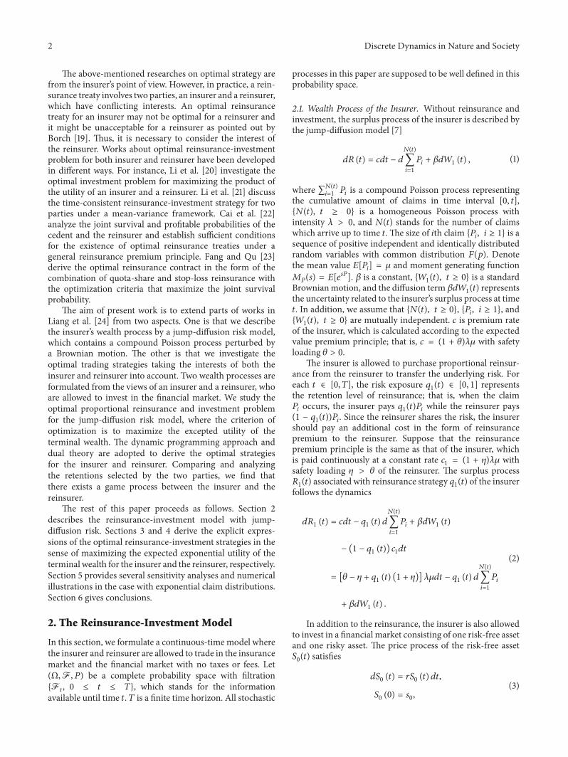
From (71) we derive that
1205971199021 (119905)120597120583 = minus119890119903(119905minus119879)12058321205741 (1 minus radic 11 + 120578) lt 01205971199022 (119905)120597120583 = 119890119903(119905minus119879)12058321205742 (1 minus radic 11 + 120578) gt 0
(73)
which implies that 119902lowast1 (119905) decreases with 120583 as it is shownin Figure 2 Figure 2 also shows that 119902lowast2 (119905) is an increasingfunction of 120583 This is that a greater 120583 means a larger claimsize
Figure 3 indicates the influence of risk-averse coefficients120574119894 on the reinsurance strategies The insurerrsquos risk aversion
10 Discrete Dynamics in Nature and Society
01
02
03
04
05
06
07
08
09
Opt
imal
rein
sura
nce s
trat
egie
sqlowast i(t)
04 06 08 1 12 1402 16
q1(t)
q2(t)
Figure 2 The effects of 120583 on 119902lowast119894 (119905)
005 01 015 02 025 03 035 04
q1(t)
q2(t)
0010203040506070809
1
Opt
imal
rein
sura
nce s
trat
egie
sqlowast i(t)
i
Figure 3 The effects of 120574119894 on 119902lowast119894 (119905)
coefficient 1205741 for exponential utility exerts a negative effecton the retention 119902lowast1 (119905) and the effect of 1205742 on 119902lowast2 (119905) is positiveFrom (71) we derive that
1205971199021 (119905)1205971205741 = minus119890119903(119905minus119879)12058312057421 (1 minus radic 11 + 120578) lt 01205971199022 (119905)1205971205742 = 119890119903(119905minus119879)12058312057422 (1 minus radic 11 + 120578) gt 0
(74)
which are consistent with the illustration in Figure 3 As therisk aversion coefficient becomes larger the insurer wouldlike to raise the reinsurance proportion to hedge risk whilethe reinsurer becomes more conservative and will accept lessreinsurance to reduce risk This can be attributed to the factthat larger 120574119894 means more risk-averse
522 Sensitivity Analysis on the Optimal Investment StrategyThe effect of 120573 on the optimal investment strategy of theinsurer with exponential utility is shown in Figures 4 and 5
0
05
1
15
2
25
3
35
4
45
Opt
imal
inve
stmen
t str
ateg
ylowast 1(t)
1 2 3 4 5 6 70t
= 0
= 05
= 1
= 2
Figure 4 When 120588 = 1 the effects of 120573 on 120587lowast1 (119905)
minus25
minus2
minus15
minus1
minus05
0
05
1
15
2
Opt
imal
inve
stmen
t str
ateg
ylowast 1(t)
1 2 3 4 5 6 70t
= 0
= 05
= 1
= 2
Figure 5 When 120588 = minus1 the effects of 120573 on 120587lowast1 (119905)
From Figure 4 we see that 120587lowast1 (119905) increases with respect tothe parameter 120573 in the case of 120588 = 1 which is due to thepositive correlation between surplus process and stock pricedynamics The larger 120573 the more uncertainty on the surplusof the insurer Thus the insurer would like to invest morein the financial market If 120588 lt 0 the correlation betweensurplus process of the insurer and stock price is negative120587lowast1 (119905) decreases with respect to 120573 see Figure 5
From (4) we know that the parameter 120590 represents thevolatility of risky asset The larger 120590 is the less wealth will beput into the risky assets as it is depicted in Figure 6
From Figure 7 we find that both 120587lowast1 (119905) and 120587lowast2 (119905) decreasewith respect to the parameter 120574119894 119894 = 1 2 As 120574119894 becomes largerthe investor is more risk adverse they will reduce the amountin the risky assets
6 Conclusion
In this paper we investigate two optimization problemswhich take both the insurer and reinsurer into account The
Discrete Dynamics in Nature and Society 11
1(t)
2(t)
minus100
0
100
200
300
400
500
Opt
imal
inve
stmen
t str
ateg
ies
lowast i(t)
01 02 03 04 05 06 070 08
Figure 6 The effects of 120590 on 120587lowast119894 (119905)
0
1
2
3
4
5
6
Opt
imal
inve
stmen
t str
ateg
ies
lowast i(t)
7
005 01 015 02 025 03 035 040i
1(t)
2(t)
Figure 7 The effects of 120574119894 on 120587lowast119894 (119905)
surplus process follows a jump-diffusion process and theinsurer purchases proportional reinsurance from the rein-surer Twowealth processes are described from the respectiveview of an insurer and a reinsurer who are allowed to investin a risky asset and a risk-free asset Applying stochastic con-trol theory we derive the corresponding Hamilton-Jacobi-Bellman equations and obtain the optimal reinsurance-investment strategies for exponential utility maximizationComparing the optimal strategies designed by two sideswe observe that the insurerrsquos reinsurance strategy is differ-ent from the reinsurerrsquos strategy The optimal reinsurancestrategies are related to the safety loading of the reinsurerand the claim sizes distribution If there exists a correlationbetween the risk model and the price of the risky asset theoptimal investment strategy is influenced by both financialmarket and insurance market Otherwise the investmentstrategy is only affected by the parameters in the financialmarket and the risk preference of the investor When theinsurer and the reinsurer have the same absolute reversionrisk coefficient the sum of two optimal proportion retentionsequals 1 which implies the conflicting interests between
the insurer and the reinsurer Finally we analyze the effectsof several parameters on the optimal strategies and presentseveral numerical simulations
Conflicts of Interest
The authors declare that there are no conflicts of interestregarding the publication of this paper
References
[1] H Schmidli ldquoOn minimizing the ruin probability by invest-ment and reinsurancerdquo The Annals of Applied Probability vol12 no 3 pp 890ndash907 2002
[2] S D Promislow and V R Young ldquoMinimizing the probabilityof ruin when claims follow Brownian motion with driftrdquo NorthAmerican Actuarial Journal vol 9 no 3 pp 109ndash128 2005
[3] Z Liang and J Guo ldquoOptimal proportional reinsurance andruin probabilityrdquo Stochastic Models vol 23 no 2 pp 333ndash3502007
[4] Y Li and G Liu ldquoDynamic proportional reinsurance andapproximations for ruin probabilities in the two-dimensionalcompound Poisson risk modelrdquo Discrete Dynamics in Natureand Society vol 2012 Article ID 802518 26 pages 2012
[5] S Luo and M Taksar ldquoOn absolute ruin minimization undera diffusion approximation modelrdquo Insurance Mathematics ampEconomics vol 48 no 1 pp 123ndash133 2011
[6] S Browne ldquoOptimal investment policies for a firm with arandom risk process exponential utility and minimizing theprobability of ruinrdquoMathematics of Operations Research vol 20no 4 pp 937ndash958 1995
[7] H Yang and L Zhang ldquoOptimal investment for insurer withjump-diffusion risk processrdquo Insurance Mathematics amp Eco-nomics vol 37 no 3 pp 615ndash634 2005
[8] L Bai and J Guo ldquoOptimal proportional reinsurance andinvestment with multiple risky assets and no-shorting con-straintrdquo Insurance Mathematics amp Economics vol 42 no 3 pp968ndash975 2008
[9] Y Cao and N Wan ldquoOptimal proportional reinsuranceand investment based on Hamilton-Jacobi-Bellman equationrdquoInsurance Mathematics amp Economics vol 45 no 2 pp 157ndash1622009
[10] N Bauerle ldquoBenchmark and mean-variance problems forinsurersrdquoMathematicalMethods of Operations Research vol 62no 1 pp 159ndash165 2005
[11] XMeng X Rong L Zhang andZDu ldquoWorst-case investmentand reinsurance optimization for an insurer under modeluncertaintyrdquoDiscrete Dynamics in Nature and Society vol 2016Article ID 9693419 8 pages 2016
[12] P Chen and S C Yam ldquoOptimal proportional reinsurance andinvestment with regime-switching for mean-variance insurersrdquoInsurance Mathematics amp Economics vol 53 no 3 pp 871ndash8832013
[13] H Zhao Y Shen and Y Zeng ldquoTime-consistent investment-reinsurance strategy for mean-variance insurers with a default-able securityrdquo Journal of Mathematical Analysis and Applica-tions vol 437 no 2 pp 1036ndash1057 2016
[14] J Cai and K S Tan ldquoOptimal retention for a stop-lossreinsurance under the VaR andCTE riskmeasuresrdquoThe Journalof the International Actuarial Association vol 37 no 1 pp 93ndash112 2007
12 Discrete Dynamics in Nature and Society
[15] J Cai K S Tan C Weng and Y Zhang ldquoOptimal reinsuranceunder VaR and CTE risk measuresrdquo Insurance Mathematics ampEconomics vol 43 no 1 pp 185ndash196 2008
[16] A Balbs B Balbs and A Heras ldquoOptimal reinsurance withgeneral risk measuresrdquo Insurance Mathematics amp Economicsvol 44 no 3 pp 374ndash384 2009
[17] K S Tan C Weng and Y Zhang ldquoVaR and CTE criteria foroptimal quota-share and stop-loss reinsurancerdquo North Ameri-can Actuarial Journal vol 13 no 4 pp 459ndash482 2009
[18] Y Chi and K S Tan ldquoOptimal reinsurance under VaR andCVaR Risk measures a simplified approachrdquo ASTIN Bulletinvol 41 no 2 pp 487ndash509 2011
[19] K Borch ldquoThe optimal reinsurance treatyrdquoASTIN Bulletin vol5 no 2 pp 293ndash297 1969
[20] D Li X Rong and H Zhao ldquoOptimal reinsurance-investmentproblem for maximizing the product of the insurerrsquos and thereinsurerrsquos utilities under a CEV modelrdquo Journal of Computa-tional and Applied Mathematics vol 255 pp 671ndash683 2014
[21] D Li X Rong and H Zhao ldquoTime-consistent reinsurance-investment strategy for an insurer and a reinsurer with mean-variance criterion under the CEV modelrdquo Journal of Computa-tional and Applied Mathematics vol 283 pp 142ndash162 2015
[22] J Cai Y Fang Z Li and G E Willmot ldquoOptimal ReciprocalReinsurance Treaties Under the Joint Survival Probability andthe Joint Profitable Probabilityrdquo Journal of Risk and Insurancevol 80 no 1 pp 145ndash168 2013
[23] Y Fang and Z Qu ldquoOptimal combination of quota-shareand stop-loss reinsurance treaties under the joint survivalprobabilityrdquo IMA Journal of Management Mathematics vol 25no 1 pp 89ndash103 2014
[24] Z Liang L Bai and J Guo ldquoOptimal investment and propor-tional reinsurance with constrained control variablesrdquo OptimalControl Applications and Methods vol 32 no 5 pp 587ndash6082011
[25] W H Soner Controlled Markov Processes and Viscosity Solu-tions Springer Berlin Germany 1993
[26] M Jonsson ldquoOptimal investment problems and volatilityhomogenization approximationsrdquo 2002
Hindawiwwwhindawicom Volume 2018
MathematicsJournal of
Hindawiwwwhindawicom Volume 2018
Mathematical Problems in Engineering
Applied MathematicsJournal of
Hindawiwwwhindawicom Volume 2018
Probability and StatisticsHindawiwwwhindawicom Volume 2018
Journal of
Hindawiwwwhindawicom Volume 2018
Mathematical PhysicsAdvances in
Complex AnalysisJournal of
Hindawiwwwhindawicom Volume 2018
OptimizationJournal of
Hindawiwwwhindawicom Volume 2018
Hindawiwwwhindawicom Volume 2018
Engineering Mathematics
International Journal of
Hindawiwwwhindawicom Volume 2018
Operations ResearchAdvances in
Journal of
Hindawiwwwhindawicom Volume 2018
Function SpacesAbstract and Applied AnalysisHindawiwwwhindawicom Volume 2018
International Journal of Mathematics and Mathematical Sciences
Hindawiwwwhindawicom Volume 2018
Hindawi Publishing Corporation httpwwwhindawicom Volume 2013Hindawiwwwhindawicom
The Scientific World Journal
Volume 2018
Hindawiwwwhindawicom Volume 2018Volume 2018
Numerical AnalysisNumerical AnalysisNumerical AnalysisNumerical AnalysisNumerical AnalysisNumerical AnalysisNumerical AnalysisNumerical AnalysisNumerical AnalysisNumerical AnalysisNumerical AnalysisNumerical AnalysisAdvances inAdvances in Discrete Dynamics in
Nature and SocietyHindawiwwwhindawicom Volume 2018
Hindawiwwwhindawicom
Dierential EquationsInternational Journal of
Volume 2018
Hindawiwwwhindawicom Volume 2018
Decision SciencesAdvances in
Hindawiwwwhindawicom Volume 2018
AnalysisInternational Journal of
Hindawiwwwhindawicom Volume 2018
Stochastic AnalysisInternational Journal of
Submit your manuscripts atwwwhindawicom
2 Discrete Dynamics in Nature and Society
The above-mentioned researches on optimal strategy arefrom the insurerrsquos point of view However in practice a rein-surance treaty involves two parties an insurer and a reinsurerwhich have conflicting interests An optimal reinsurancetreaty for an insurer may not be optimal for a reinsurer andit might be unacceptable for a reinsurer as pointed out byBorch [19] Thus it is necessary to consider the interest ofthe reinsurer Works about optimal reinsurance-investmentproblem for both insurer and reinsurer have been developedin different ways For instance Li et al [20] investigate theoptimal investment problem for maximizing the product ofthe utility of an insurer and a reinsurer Li et al [21] discussthe time-consistent reinsurance-investment strategy for twoparties under a mean-variance framework Cai et al [22]analyze the joint survival and profitable probabilities of thecedent and the reinsurer and establish sufficient conditionsfor the existence of optimal reinsurance treaties under ageneral reinsurance premium principle Fang and Qu [23]derive the optimal reinsurance contract in the form of thecombination of quota-share and stop-loss reinsurance withthe optimization criteria that maximize the joint survivalprobability
The aim of present work is to extend parts of works inLiang et al [24] from two aspects One is that we describethe insurerrsquos wealth process by a jump-diffusion risk modelwhich contains a compound Poisson process perturbed bya Brownian motion The other is that we investigate theoptimal trading strategies taking the interests of both theinsurer and reinsurer into account Two wealth processes areformulated from the views of an insurer and a reinsurer whoare allowed to invest in the financial market We study theoptimal proportional reinsurance and investment problemfor the jump-diffusion risk model where the criterion ofoptimization is to maximize the excepted utility of theterminal wealth The dynamic programming approach anddual theory are adopted to derive the optimal strategiesfor the insurer and reinsurer Comparing and analyzingthe retentions selected by the two parties we find thatthere exists a game process between the insurer and thereinsurer
The rest of this paper proceeds as follows Section 2describes the reinsurance-investment model with jump-diffusion risk Sections 3 and 4 derive the explicit expres-sions of the optimal reinsurance-investment strategies in thesense of maximizing the expected exponential utility of theterminal wealth for the insurer and the reinsurer respectivelySection 5 provides several sensitivity analyses and numericalillustrations in the case with exponential claim distributionsSection 6 gives conclusions
2 The Reinsurance-Investment Model
In this section we formulate a continuous-timemodel wherethe insurer and reinsurer are allowed to trade in the insurancemarket and the financial market with no taxes or fees Let(ΩF 119875) be a complete probability space with filtrationF119905 0 le 119905 le 119879 which stands for the informationavailable until time 119905 119879 is a finite time horizon All stochastic
processes in this paper are supposed to be well defined in thisprobability space
21 Wealth Process of the Insurer Without reinsurance andinvestment the surplus process of the insurer is described bythe jump-diffusion model [7]
119889119877 (119905) = 119888119889119905 minus 119889119873(119905)sum119894=1
119875119894 + 1205731198891198821 (119905) (1)
where sum119873(119905)119894=1 119875119894 is a compound Poisson process representingthe cumulative amount of claims in time interval [0 119905]119873(119905) 119905 ge 0 is a homogeneous Poisson process withintensity 120582 gt 0 and 119873(119905) stands for the number of claimswhich arrive up to time 119905 The size of 119894th claim 119875119894 119894 ge 1 is asequence of positive independent and identically distributedrandom variables with common distribution 119865(119901) Denotethe mean value 119864[119875119894] = 120583 and moment generating function119872119875(119904) = 119864[119890119904119875] 120573 is a constant 1198821(119905) 119905 ge 0 is a standardBrownianmotion and the diffusion term 1205731198891198821(119905) representsthe uncertainty related to the insurerrsquos surplus process at time119905 In addition we assume that 119873(119905) 119905 ge 0 119875119894 119894 ge 1 and1198821(119905) 119905 ge 0 are mutually independent 119888 is premium rateof the insurer which is calculated according to the expectedvalue premium principle that is 119888 = (1 + 120579)120582120583 with safetyloading 120579 gt 0
The insurer is allowed to purchase proportional reinsur-ance from the reinsurer to transfer the underlying risk Foreach 119905 isin [0 119879] the risk exposure 1199021(119905) isin [0 1] representsthe retention level of reinsurance that is when the claim119875119894 occurs the insurer pays 1199021(119905)119875119894 while the reinsurer pays(1 minus 1199021(119905))119875119894 Since the reinsurer shares the risk the insurershould pay an additional cost in the form of reinsurancepremium to the reinsurer Suppose that the reinsurancepremium principle is the same as that of the insurer whichis paid continuously at a constant rate 1198881 = (1 + 120578)120582120583 withsafety loading 120578 gt 120579 of the reinsurer The surplus process1198771(119905) associated with reinsurance strategy 1199021(119905) of the insurerfollows the dynamics
1198891198771 (119905) = 119888119889119905 minus 1199021 (119905) 119889119873(119905)sum119894=1
119875119894 + 1205731198891198821 (119905)minus (1 minus 1199021 (119905)) 1198881119889119905
= [120579 minus 120578 + 1199021 (119905) (1 + 120578)] 120582120583119889119905 minus 1199021 (119905) 119889119873(119905)sum119894=1
119875119894+ 1205731198891198821 (119905)
(2)
In addition to the reinsurance the insurer is also allowedto invest in a financial market consisting of one risk-free assetand one risky asset The price process of the risk-free asset1198780(119905) satisfies
1198891198780 (119905) = 1199031198780 (119905) 1198891199051198780 (0) = 1199040 (3)
Discrete Dynamics in Nature and Society 3
where 119903 gt 0 is the risk-free interest rate The price processof the risky asset 119878(119905) is described by the geometric Brownianmotion
119889119878 (119905) = 120572119878 (119905) 119889119905 + 120590119878 (119905) 119889119882 (119905) 119878 (0) = 119904 (4)
where 120572 gt 119903 and 120590 are positive constants 119882(119905) is anotherstandard Brownian motion defined on (ΩF 119875) which isrelated to 1198821(119905) by 119864[1198891198821(119905)119882(119905)] = 120588119889119905 and 120588 isin [minus1 1]is the correlation coefficient
Let 1205871(119905) be the amount of the wealth invested in the riskyasset at time 119905 by the insurer Then the remainder 119883(119905) minus1205871(119905) is invested in the risk-free asset Since the insurer isallowed to purchase reinsurance and invest in the financialmarket the trading strategy is a pair of stochastic processesΠ1 fl (1199021(119905) 1205871(119905)) 119905 isin [0 119879] where 1199021(119905) representsthe reinsurance strategy and 1205871(119905) represents the investmentstrategy The reinsurance-investment strategyΠ1(119905) is said tobe admissible if it isF119905-progressivelymeasurable and satisfies0 le 1199021(119905) le 1 119864[int119879
012058721(119905)119889119905] lt infin Corresponding to an
admissible reinsurance-investment strategyΠ1 and the initialwealth 119883(0) = 119909 the wealth process 119883(119905) of the insurerfollows the stochastic differential equation
119889119883 (119905) = 1198891198771 (119905) + 1205871 (119905) 119889119878 (119905)119878 (119905) + (119883 (119905)minus 1205871 (119905)) 1198891198780 (119905)1198780 (119905) = [119903119883 (119905) + (120572 minus 119903) 1205871 (119905)+ (120579 minus 120578) 120582120583 + 1199021 (119905) (1 + 120578) 120582120583] 119889119905minus 1199021 (119905) 119889119873(119905)sum
119894=1
119875119894 + 1205731198891198821 (119905) + 1205901205871 (119905) 119889119882 (119905)
(5)
Suppose that the utility function 1198801(sdot) is concave andcontinuously differentiable on 119877 The objective of the insureris assumed to maximize the expected utility of terminalwealth 119883(119879) that is
max11990211205871
119864 [1198801 (119883 (119879))] (6)
subject to (5)
22 Wealth Process of the Reinsurer In the presence of theproportional reinsurance contract the surplus process 1198772(119905)of the reinsurer satisfies
1198891198772 (119905) = (1 minus 1199022 (119905)) (1 + 120578) 120582120583119889119905minus (1 minus 1199022 (119905)) 119889119873(119905)sum
119894=1
119875119894 (7)
where 1199022(119905) is the reinsurance strategy chosen by the rein-surer Generally the reinsurer will accept the reinsuranceproportion proposed by the insurer when the retention levelof the reinsurer is smaller than that of the insurer while in the
opposite case in order to prevent large losses the reinsurermay not accept the reinsurance strategy given by the insurer
Let 1205872(119905) be the amount of the wealth invested in therisky asset at time 119905 by the reinsurer Then the remainder119884(119905) minus 1205871(119905) is invested in the risk-free asset Similar to theinsurer the trading strategy of the reinsurer is also a pair ofprocesses Π2 fl (1199022(119905) 1205872(119905)) 119905 isin [0 119879] where 1199022(119905) and1205872(119905) represent the reinsurance strategy and the investmentstrategy respectively The reinsurance-investment strategyΠ2(119905) is said to be admissible if it is F119905-progressivelymeasurable and satisfies 0 le 1199022(119905) le 1 119864[int119879
012058722(119905)119889t] ltinfin Corresponding to an admissible reinsurance-investment
strategy Π2 and the initial wealth 119884(0) = 119910 the wealthprocess119884(119905) of the reinsurer follows the stochastic differentialequation
119889119884 (119905)= [119903119884 (119905) + (120572 minus 119903) 1205872 (119905) + 120582120583 (1 minus 1199022 (119905)) (1 + 120578)] 119889119905
minus (1 minus 1199022 (119905)) 119889119873(119905)sum119894=1
119875119894 + 1205901205872 (119905) 119889119882 (119905) (8)
Suppose that the utility function1198802(sdot) is concave and con-tinuously differentiable on 119877 The objective of the reinsurer isassumed to maximize the expected utility of terminal wealth119884(119879) that is
max11990221205872
119864 [1198802 (119884 (119879))] (9)
subject to (8)
3 Optimal Strategy for the Insurer
Assume that the insurer takes an exponential utility function
1198801 (119909) = 1205821 minus 1198981205741 119890minus1205741119909 1205821 119898 gt 0 (10)
where 1205741 gt 0 represents the absolute risk aversion coefficientThe exponential utility plays a prominent role in insurancemathematics and actuarial practice It is the only utilityfunction under which the principle of ldquozero utilityrdquo gives afair premium that is dependent on the level of reserve of aninsurance company
For an admissible strategy (1199021 1205871) isin Π1 define the valuefunction
119867(119905 119909) = sup(1199021 1205871)
119864 [1198801 (119883 (119879)) | 119883 (119905) = 119909] 0 le 119905 le 119879 (11)
with 119867(119879 119909) = 1198801(119909) According to works of Soner [25] ifthe value function 119867(119905 119909) and its partial derivatives 119867119905 119867119909
4 Discrete Dynamics in Nature and Society
and 119867119909119909 are continuous on [0 119879] times 119877+ then 119867(119905 119909) satisfiesthe following Hamilton-Jacobi-Bellman (HJB) equation
119867119905 + [119903119909 + (120579 minus 120578) 120582120583]119867119909 + 12057322 119867119909119909+ sup1205871(119905)ge0
(120572 minus 119903) 1205871 (119905)119867119909+ (12120590212058721 (119905) + 1205881205731205901205871 (119905))119867119909119909+ sup1199021(119905)isin[01]
1199021 (119905) (1 + 120578) 120582120583119867119909+ 120582119864 [119867 (119905 119909 minus 1199021 (119905) 119875) minus 119867 (119905 119909)] = 0
(12)
with boundary condition 119867(119879 119909) = 1198801(119909) for any (119905 119909) isin[0 119879) times 119877+Differentiating (12) with respect to 1205871(119905) and setting the
derivatives equal to zero we have
(120572 minus 119903)119867119909 + (12059021205871 (119905) + 120588120573120590)119867119909119909 = 0 (13)
The first-order maximizing condition for the insurerrsquos invest-ment strategy 1205871(119905) yields
120587lowast (119905) = minus1205881205731205901205902 minus 120572 minus 1199031205902 119867119909119867119909119909 (14)
Substituting (14) into the left-hand side of the HJB equation(12) we obtain
119867119905 + [119903119909 + (120579 minus 120578) 120582120583]119867119909 + 12057322 119867119909119909minus [(120572 minus 119903)119867119909 + 120588120573120590119867119909119909]221205902119867119909119909+ sup1199021(119905)isin[01]
1199021 (119905) (1 + 120578) 120582120583119867119909+ 120582119864 [119867 (119905 119909 minus 1199021 (119905) 119875) minus 119867 (119905 119909)] = 0
(15)
with 119867(119879 119909) = 1198801(119909) We construct a solution for (15) in thefollowing form
119867(119905 119909) = 1205821 minus 1198981205741 exp [minus1205741119909119890119903(119879minus119905) + ℎ (119879 minus 119905)] (16)
where ℎ(sdot) is a suitable function such that expression (16) isa solution of (15) The boundary condition 119867(119879 119909) = 1198801(119909)implies ℎ(119879) = 0 From (16) we have
119867119905 = (119867 (119905 119909) minus 1205821) [1205741119909119903119890119903(119879minus119905) minus ℎ1015840 (119879 minus 119905)] 119867119909 = (119867 (119905 119909) minus 1205821) [minus1205741119890119903(119879minus119905)] 119867119909119909 = (119867 (119905 119909) minus 1205821) [120574211198902119903(119879minus119905)] 119864 [119867 (119905 119909 minus 1199021 (119905) 119875) minus 119867 (119905 119909)]
= (119867 (119905 119909) minus 1205821) [119872119875 (12057411199021 (119905) 119890119903(119879minus119905)) minus 1]
(17)
Substituting (17) into (15) yields
119867119905 + [119903119909 + (120579 minus 120578) 120582120583]119867119909 + 12057322 119867119909119909minus [(120572 minus 119903)119867119909 + 120588120573120590119867119909119909]221205902119867119909119909 + sup
1199021(119905)isin[01]
119891 (1199021 (119905))= 0
(18)
where
119891 (1199021 (119905)) = 120582 (119867 (119905 119909) minus 1205821)sdot [minus1205831205741 (1 + 120578) 1199021 (119905) 119890119903(119879minus119905) + 119872119875 (12057411199021 (119905) 119890119903(119879minus119905))minus 1]
(19)
Differentiating (19) with respect to 1199021(119905) we get120597119891 (1199021 (119905))1205971199021 (119905) = 1205821205741119890119903(119879minus119905) (119867 (119905 119909) minus 1205821)
sdot [minus120583 (1 + 120578) + 119864 [11987511989012057411199021(119905)119875119890119903(119879minus119905)]] 1205972119891 (1199021 (119905))12059711990221 (119905) = 120582120574211198902119903(119879minus119905) (119867 (119905 119909) minus 1205821)
sdot 119864 [119875211989012057411199021(119905)119875119890119903(119879minus119905)] lt 0
(20)
Thus 119891(1199021(119905)) is concave and its maximizer 1199021(119905) satisfies theequation
(1 + 120578) 120583 = 119864 [11987511989012057411199021(119905)119875119890119903(119879minus119905)] = 1198721015840119875 (120598) (21)
where 120598 fl 12057411199021(119905)119890119903(119879minus119905)Lemma 1 Equation (21) has a unique positive root 120598Proof Let
V (120598) = (1 + 120578) 120583 minus 1198721015840119875 (120598) (22)
From
V1015840 (120598) = minus119864 [1198752119890120598119875] lt 0V10158401015840 (120598) = minus119864 [1198753119890120598119875] lt 0 (23)
we know that V(120598) is a decreasing concave functionMoreoverV(0) = 120583120578 gt 0 Thus V(120598) has a unique point of intersectionwith the abscissa axis which implies that (21) has a uniquepositive solution 120598
Note that 1199021(119905) = (1205981205741)119890minus119903(119879minus119905) and the optimal rein-surance proportion 119902lowast1 (119905) isin [0 1] If 0 le 1199021(119905) le 1 theoptimal reinsurance proportion 119902lowast1 (119905) coincides with 1199021(119905) If1199021(119905) le 0 we let 119902lowast1 (119905) = 0 If 1199021(119905) ge 1 we set 119902lowast1 (119905) = 1In this paper 1199021(119905) = 0 means that the reinsurer takes all
Discrete Dynamics in Nature and Society 5
the insurance risk and the insurer acts as a middleman inthe process of the insurance From Lemma 1 120598 is a positiveconstant which depends on the safety loading 120578 and theclaim sizes distribution 119865(119901) Therefore 1199021(119905) ge 0 and wediscuss the optimal reinsurance strategy for the insurer in thefollowing three cases
When 120598 le 1205741 we have 1205981205741 le 1 and 1199021(119905) =(1205981205741)119890minus119903(119879minus119905) le 1 for any 119905 isin [0 119879] Then the optimalreinsurance strategy is 119902lowast1 (119905) = 1199021(119905) 0 le 119905 le 119879
When 1205741 le 120598 le 1205741119890119903119879 we have 1205981205741 gt 1 Let 1199050 = 119879 +(1119903) ln(1205741120598) Then 1199021(119905) = (1205981205741)119890minus119903(119879minus119905) lt 1 for 119905 isin [0 1199050]
and 1199021(119905) ge 1 for 119905 isin [1199050 119879] the optimal reinsurance strategyis
119902lowast1 (119905) = 1199021 (119905) 0 le 119905 le 11990501 1199050 le 119905 le 119879 (24)
When 120598 ge 1205741119890119903119879 we have 1199021(119905) = (1205981205741)119890minus119903(119879minus119905) ge 119890119903119905 ge 1for any 119905 isin [0 119879] Then the optimal reinsurance strategy is119902lowast1 (119905) = 1 0 le 119905 le 119879
Substituting 119902lowast1 (119905) into (19) the value of 119891(119902lowast1 (119905)) is givenby
119891 (119902lowast1 (119905)) = 120582 (119867 (119905 119909) minus 1205821) [minus120598120583 (1 + 120578) + 119872119875 (120598) minus 1] 119902lowast1 (119905) = 1199021 (119905) 120582 (119867 (119905 119909) minus 1205821) [minus120598120583 (1 + 120578) + 119872119875 (120598) minus 1] 119902lowast1 (119905) = 1 (25)
where 120598 fl 1205741119890119903(119879minus119905)Replacing the supremum in (18) by 119891(119902lowast1 (119905)) yields the
following equation
119867119905 + [119903119909 + (120579 minus 120578) 120582120583]119867119909 + 12057322 119867119909119909minus [(120572 minus 119903)119867119909 + 120588120573120590119867119909119909]221205902119867119909119909 + 119891 (119902lowast1 (119905)) = 0
(26)
Here the stochastic optimal control problem describedabove has been transformed into solving a partial differentialequation for the value function 119867(119905 119909) We intent to find thesolution to (26) with boundary condition119867(119879 119909) = 1198801(119909) byusing Legendre transformation and variables changemethod
Definition 2 (see [26]) Let 119867 119877 rarr 119877 be a convex functionFor 119911 gt 0 define the Legendre transform
119871 (119911) = sup119909gt0
119867 (119909) minus 119911119909 (27)
The function 119871(119911) is called the Legendre dual of function119867(119909)Following the works in [26] we define a Legendre
transform
(119905 119911) = sup119909gt0
119867 (119905 119909) minus 119911119909 119905 isin [0 119879] 119892 (119905 119911) = inf
119909gt0119909 | 119867 (119905 119909) ge 119911119909 + (119905 119911)
119905 isin [0 119879] (28)
where 119911 gt 0 denotes the dual variable to 119909 The function(119905 119911) is related to 119892(119905 119911) by119892 (119905 119911) = minus119911 (119905 119911) (29)
Noting that 119867(119879 119909) = 1198801(119909) at terminal time 119879 we have (119879 119911) = sup
119909gt0
1198801 (119909) minus 119911119909 119892 (119879 119911) = inf
119909gt0119909 | 1198801 (119909) ge 119911119909 + (119879 119911) (30)
from which we get
119892 (119879 119911) = (11988010158401)minus1 (119911) (31)
Equation (31) shows that 119892(119879 119911) is the inverse of marginalutility
Using (28) we derive 119867119909(119905 119909) = 119911 and119892 (119905 119911) = 119909 (119905 119911) = 119867 (119905 119892) minus 119911119892 (32)
Referring to [26] we get the following transformation rules
119867119905 = 119905119867119909119909 = minus 1
119867119911119911 (33)
where = (119905 119911) Substituting (33) into (26) we have119905 + [119903119892 (119905 119911) + (120579 minus 120578) 120582120583] 119911 + 1205732 (1 minus 1205882)
2 119867119909119909minus (120572 minus 119903)2 119911211991111991121205902 minus 120588120573 (120572 minus 119903) 119911120590+ 120582 ( (119905 119911) + 119911119892 (119905 119911) minus 1205821) 1198911 (119902lowast1 (119905)) = 0
(34)
where1198911 (119902lowast1 (119905))
= minus120598120583 (1 + 120578) + 119872119875 (120598) minus 1 119902lowast1 (119905) = 1199021 (119905) minus120598120583 (1 + 120578) + 119872119875 (120598) minus 1 119902lowast1 (119905) = 1
(35)
6 Discrete Dynamics in Nature and Society
Letting 1205882 = 1 and differentiating (34) with respect to 119911 yields119892119905 (119905 119911) minus 119903119892 (119905 119911)
+ [(120572 minus 119903)21205902 minus 119903 minus 1205821198911 (119902lowast1 (119905))] 119911119892119911 (119905 119911)+ (120572 minus 119903)2 119911221205902 119892119911119911 (119905 119911) + 120588120573 (120572 minus 119903)120590minus (120579 minus 120578) 120582120583 = 0
(36)
with boundary condition 119892(119879 119911) = (11988010158401)minus1(119911)The optimal investment strategy (14) is in the form
120587lowast (119905) = minus1205881205731205901205902 minus 120572 minus 1199031205902 119911119892119911 (119905 119911) (37)
The problem now is to solve (36) for the dual 119892(119905 119911) andreplace it in (37) so as to obtain the optimal strategy
From the exponential utility function given by (10) and(31) the boundary condition is expressed as
119892 (119879 119911) = minus 11205741 ln119911119898 (38)
Thus we try to conjecture a solution to (36) in the form
119892 (119905 119911) = minus119886 (119905)1205741 ln 119911119898 + 119887 (119905) (39)
with 119886(119879) = 1 and 119887(119879) = 0 Then we have
119892119905 (119905 119911) = minus1198861015840 (119905)1205741 ln 119911119898 + 1198871015840 (119905) 119892119911 (119905 119911) = minus119886 (119905)1205741119911 119892119911119911 (119905 119911) = 119886 (119905)12057411199112
(40)
Substituting (40) into (36) yields
minus ln (119911119898)1205741 1198861015840 (119905) + 1198871015840 (119905) + 119903 ln (119911119898)1205741 119886 (119905) minus 119903119887 (119905)minus [(120572 minus 119903)221205902 minus 119903 minus 1205821198911 (119902lowast1 (119905))] 119886 (119905)1205741+ 120588120573 (120572 minus 119903)120590 minus (120579 minus 120578) 120582120583 = 0
(41)
We split (41) into two equations
1198861015840 (119905) minus 119903119886 (119905) = 01198871015840 (119905) minus 119903119887 (119905) minus [(120572 minus 119903)221205902 minus 119903 minus 1205821198911 (119902lowast1 (119905))] 119886 (119905)1205741
+ 120588120573 (120572 minus 119903)120590 minus (120579 minus 120578) 120582120583 = 0(42)
Taking the boundary conditions 119886(119879) = 1 and 119887(119879) = 0 intoaccount the solutions to (42) are
119886 (119905) = 119890119903(119905minus119879)119887 (119905) = 119860 (1 minus 119890119903(119905minus119879))
119903 + 119861 (119905 minus 119879)1205741 119890119903(119905minus119879) (43)
where 119860 = 120588120573(120572 minus 119903)120590 minus (120579 minus 120578)120582120583 and 119861 = (120572 minus 119903)221205902 minus119903 minus 1205821198911(119902lowast1 (119905))The above derivations lead to the following theorem
Theorem 3 Assume that the insurer takes an exponentialutility function in the form of (10) Let 1199050 = 119879 + (1119903) ln(1205741120598)and 1205882 = 1 the optimal reinsurance-investment strategies forthe insurer are given as follows
(1) If 120598 le 1205741 the optimal reinsurance strategy is 119902lowast1 (119905) =(1205981205741)119890minus119903(119879minus119905) 0 le 119905 le 119879(2) If 1205741 le 120598 le 1205741119890119903119879 the optimal reinsurance strategy is
119902lowast1 (119905) = 1205981205741 119890minus119903(119879minus119905) 0 le 119905 le 11990501 1199050 le 119905 le 119879 (44)
(3) If 120598 ge 1205741119890119903119879 the optimal reinsurance strategy is 119902lowast1 (119905) =1 0 le 119905 le 119879where 120598 is the unique positive root to (21) The correspondingoptimal investment strategy is
120587lowast1 (119905) = 120588120573120590 + 120572 minus 1199031205902 119890119903(119905minus119879)1205741 0 le 119905 le 119879 (45)
4 Optimal Strategy for the Reinsurer
In this section we discuss the optimal strategy for thereinsurer Suppose that the utility function of the reinsureris given by
1198802 (119910) = 1205821 minus 1198981205742 119890minus1205742119910 1205742 gt 0 119898 gt 0 (46)
where 1205742 represents the absolute risk aversion coefficient forthe reinsurer
For an admissible strategy (1199022 1205872) isin Π2 the valuefunction for the reinsurer is defined in the form
119867(119905 119910) = sup(1199022 1205872)
119864 [1198802 (119884 (119879)) | 119884 (119905) = 119910] 0 le 119905 le 119879 (47)
Discrete Dynamics in Nature and Society 7
with 119867(119879 119910) = 1198802(119910) The corresponding Hamilton-Jacobi-Bellman (HJB) equation is
119867119905 + [119903119910 + 120582120583 (1 + 120578)]119867119910 + sup1205872(119905)
(120572 minus 119903) 1205872 (119905)119867119910+ 12120590212058722 (119905)119867119910119910 + sup
1199022(119905)
minus120582120583 (1 + 120578) 1199022 (119905)119867119910+ 120582119864 [119867 (119905 119910 minus (1 minus 1199022 (119905)) 119875) minus 119867 (119905 119910)] = 0
(48)
with the boundary condition119867(119879 119910) = 1198802(119910) where119867119905119867119910and 119867119910119910 denote partial derivatives of 119867 = 119867(119905 119910) The first-order maximizing condition for the investment strategy 1205872(119905)yields
120587lowast2 (119905) = minus120572 minus 1199031205902119867119910119867119910119910 (49)
Substituting the optimal investment strategy 120587lowast2 (119905) into theHJB equation (48) we derive that
119867119905 + [119903119910 + 120582120583 (1 + 120578)]119867119910 minus (120572 minus 119903)2212059021198672119910119867119910119910
+ sup1199022(119905)
minus120582120583 (1 + 120578) 1199022 (119905)119867119910+ 120582119864 [119867 (119905 119910 minus (1 minus 1199022 (119905)) 119875) minus 119867 (119905 119910)] = 0
(50)
We formulate a solution for (50) in the form
119867(119905 119910) = 1205821 minus 1198981205742 exp [minus1205742119910119890119903(119879minus119905) + 119896 (119879 minus 119905)] (51)
where 119896(sdot) is a suitable function such that formulation (51) isa solution of (50) The boundary condition 119867(119879 119910) = 1198802(119910)implies 119896(119879) = 0 Using (51) we have
119867119905 = (119867 (119905 119910) minus 1205821) [1205742119910119903119890119903(119879minus119905) minus 1198961015840 (119879 minus 119905)] 119867119910 = (119867 (119905 119910) minus 1205821) [minus1205742119890119903(119879minus119905)] 119867119910119910 = (119867 (119905 119910) minus 1205821) [120574221198902119903(119879minus119905)] 119864 [119867 (119905 119910 minus (1 minus 1199022 (119905)) 119875) minus 119867 (119905 119910)]
= (119867 (119905 119910) minus 1205821) [119872119875 (1205742 (1 minus 1199022 (119905)) 119890119903(119879minus119905)) minus 1]
(52)
Substituting (52) into (50) gives rise to
119867119905 + [119903119910 + 120582120583 (1 + 120578)]119867119910 minus (120572 minus 119903)2212059021198672119910119867119910119910
+ sup1199022(119905)
119891 (1199022 (119905)) = 0(53)
where
119891 (1199022 (119905)) = 120582 (119867 (119905 119910) minus 1205821) [1205742120583 (1 + 120578) 1199022 (119905) 119890119903(119879minus119905)+ 119872119875 (1205742 (1 minus 1199022 (119905)) 119890119903(119879minus119905)) minus 1] (54)
Differentiating (54) with respect to 1199022(119905) we get120597119891 (1199022 (119905))1205971199022 (119905) = 1205821205742119890119903(119879minus119905) (119867 (119905 119910) minus 1205821)
sdot [120583 (1 + 120578) minus 119864 [1198751198901205742(1minus1199022(119905))119875119890119903(119879minus119905)]] 1205972119891 (1199022 (119905))12059711990222 (119905) = 120582120574221198902119903(119879minus119905) (119867 (119905 119910) minus 1205821)
sdot 119864 [11987521198901205742(1minus1199022(119905))119875119890119903(119879minus119905)] lt 0
(55)
Thus 119891(1199022(119905)) is concave and its maximizer 1199022(119905) satisfies theequation
120583 (1 + 120578) = 119864 [1198751198901205742(1minus1199022(119905))119875119890119903(119879minus119905)] = 1198721015840119875 (120598) (56)
where 120598 fl 1205742(1 minus 1199022(119905))119890119903(119879minus119905)From Lemma 1 there exists a unique positive root 120598 for
(56) Therefore we have 1199022(119905) = 1 minus (1205981205742)119890minus119903(119879minus119905) le 1 Recallthat the optimal reinsurance proportion 119902lowast2 (119905) isin [0 1] If 0 le1199022(119905) le 1 the optimal reinsurance proportion 119902lowast2 (119905) coincideswith 1199022(119905) If 1199022(119905) le 0 we let 119902lowast2 (119905) = 0 If 1199022(119905) ge 1 we set119902lowast2 (119905) = 1 The optimal reinsurance strategy for the reinsureris discussed in the following three cases
When 120598 le 1205742 we have 1 minus 1205981205742 ge 0 and 1199022(119905) =1 minus (1205981205742)119890minus119903(119879minus119905) ge 0 for any 119905 isin [0 119879] Then the optimalreinsurance strategy is 119902lowast2 (119905) = 1199022(119905) 0 le 119905 le 119879
When 1205742 le 120598 le 1205742119890119903119879 we have 1 minus 1205981205741 lt 0 Let 1199050 =119879 + (1119903) ln(1205742120598) Then 1199022(119905) = 1 minus (1205981205742)119890minus119903(119879minus119905) gt 0 for 119905 isin[0 1199050] and 1199022(119905) le 0 for 119905 isin [1199050 119879] the optimal reinsurancestrategy is
119902lowast2 (119905) = 1199022 (119905) 0 le 119905 le 11990500 1199050 le 119905 le 119879 (57)
When 120598 ge 1205742119890119903119879 we have 1199022(119905) = 1 minus (1205981205742)119890minus119903(119879minus119905) le1 minus (1205981205742)119890minus119903119879 lt 0 for any 119905 isin [0 119879] Then the optimalreinsurance strategy is 119902lowast2 (119905) = 0 0 le 119905 le 119879
8 Discrete Dynamics in Nature and Society
Substituting 119902lowast2 (119905) into (54) the value of 119891(119902lowast2 (119905)) isexpressed as
119891 (119902lowast2 (119905)) = 120582 (119867 (119905 119910) minus 1205821) [120583 (1 + 120578) (120598 minus 120598) + 119872119875 (120598) minus 1] 119902lowast2 (119905) = 1199022 (119905) 120582 (119867 (119905 119910) minus 1205821) [119872119875 (120598) minus 1] 119902lowast2 (119905) = 0 (58)
where 120598 fl 1205742119890119903(119879minus119905)Replacing the supremum in (53) by 119891(119902lowast2 (119905)) yields
119867119905 + [119903119910 + 120582120583 (1 + 120578)]119867119910 minus (120572 minus 119903)2212059021198672119910119867119910119910
+ 120582 (119867 (119905 119910) minus 1205821) 1198912 (119902lowast2 (119905)) = 0(59)
where
1198912 (119902lowast2 (119905))=
120583 (1 + 120578) (120598 minus 120598) + 119872119875 (120598) minus 1 119902lowast2 (119905) = 1199022 (119905) 119872119875 (120598) minus 1 119902lowast2 (119905) = 0
(60)
Using the approach of Legendre transform we derive thatthe dual equation of (59) is
119892119905 (119905 119911) minus 119903119892 (119905 119911)+ [(120572 minus 119903)21205902 minus 119903 minus 1205821198912 (119902lowast2 (119905))] 119911119892119911 (119905 119911)+ (120572 minus 119903)2 119911221205902 119892119911119911 (119905 119911) minus 120582120583 (1 + 120578) = 0
(61)
with boundary condition 119892(119879 119911) = (11988010158402)minus1(119911)From the exponential utility given by (46) and the dual
equation (61) we set that the boundary condition is
119892 (119879 119911) = minus 11205742 ln119911119898 (62)
Suppose that a solution to (61) has the form
119892 (119905 119911) = minus119894 (119905)1205742 ln 119911119898 + 119895 (119905) (63)
with 119894(119879) = 1 and 119895(119879) = 0 We have
119892119905 (119905 119911) = minus1198941015840 (119905)1205742 ln 119911119898 + 1198951015840 (119905) 119892119911 (119905 119911) = minus119894 (119905)1205742119911 119892119911119911 (119905 119911) = 119894 (119905)12057421199112
(64)
Substituting (64) into (61) we get
minus ln (119911119898)1205742 1198941015840 (119905) + 1198951015840 (119905) + 119903 ln (119911119898)1205742 119894 (119905) minus 119903119895 (119905)minus [(120572 minus 119903)221205902 minus 119903 minus 1205821198912 (119902lowast2 (119905))] 119894 (119905)1205742minus (1 + 120578) 120582120583 = 0
(65)
We decompose (65) into two equations
1198941015840 (119905) minus 119903119894 (119905) = 01198951015840 (119905) minus 119903119895 (119905) minus [(120572 minus 119903)221205902 minus 119903 minus 1205821198912 (119902lowast2 (119905))] 119894 (119905)1205742
minus (1 + 120578) 120582120583 = 0(66)
Taking the boundary conditions 119894(119879) = 1 and 119895(119879) = 0 intoaccount the solutions to (66) are
119894 (119905) = 119890119903(119905minus119879)119895 (119905)
= minus (1 + 120578) 120582120583 (1 minus 119890119903(119905minus119879))119903
+ [(120572 minus 119903)221205902 minus 119903 minus 1205821198912 (119902lowast2 (119905))] (119905 minus 119879) 119890119903(119905minus119879)1205742
(67)
The above derivations lead to the following theorem
Theorem 4 Assume that the reinsurer takes an exponentialutility function in the form of (46) Let 1199050 = 119879 + (1119903) ln(1205742120598)the optimal reinsurance-investment strategies for the reinsurerare given as follows
(1) If 120598 le 1205742 the optimal reinsurance strategies is 119902lowast2 (119905) =1 minus (1205981205742)119890minus119903(119879minus119905) 0 le 119905 le 119879(2) If 1205742 le 120598 le 1205742119890119903119879 the optimal reinsurance strategy is
119902lowast2 (119905) = 1 minus 1205981205742 119890minus119903(119879minus119905) 0 le 119905 le 11990500 1199050 le 119905 le 119879 (68)
(3) If 120598 ge 1205742119890119903119879 the optimal reinsurance strategy is 119902lowast2 (119905) =0 0 le 119905 le 119879
Discrete Dynamics in Nature and Society 9
where 120598 is the unique positive root to (56) The correspondingoptimal investment strategy for the reinsurer is
120587lowast2 (119905) = 120572 minus 1199031205902 119890119903(119905minus119879)1205742 0 le 119905 le 119879 (69)
5 Comparative Analyses andNumerical Illustrations
51 Comparative Analyses on 119902lowast1 (119905) and 119902lowast2 (119905) A fair reinsur-ance contract should consider the interests of both insurerand reinsurer while they both prefer to choose a reinsuranceproportion for their own utility maximization Assume thatthe insurer and the reinsurer have complete information onthe risk of insurance and investment If the optimal retentionlevel chosen by the insurer is larger than that of the reinsurerthe reinsurer will accept the strategy But in the oppositecase the reinsurer may oppose the contract proposed by theinsurer When 1205741 = 1205742 according to their wealth processesthe sum of two optimal reinsurance ratios chosen by insurerand the reinsurer equals 1 which reflects the game betweenthe insurer and the reinsurer
We give specialized analyses on 119902lowast1 (119905) = 119902lowast2 (119905) 119902lowast1 (119905) gt119902lowast2 (119905) and 119902lowast1 (119905) lt 119902lowast2 (119905) When 119902lowast1 (119905) = 119902lowast2 (119905) the insurerand reinsurer reach a consensus on the retention proportionand they both obtain the maximum value of terminal wealththe insurance contract is established When 119902lowast1 (119905) gt 119902lowast2 (119905)the insurerrsquos retention proportion is larger than that of thereinsurerThe insurer prefers to purchase less reinsurance andundertake more risk himself while the reinsurer is willingto accept a higher level of reinsurance When 119902lowast1 (119905) lt 119902lowast2 (119905)the insurerrsquos retention proportion is smaller than that of thereinsurer The insurer would like to spread more risks tothe reinsurer which is unacceptable for the reinsurer Theinsurer may need to find other reinsurers to undertake therest 119902lowast2 (119905) minus 119902lowast1 (119905) proportion of reinsurance
52 Sensitivity Analyses and Numerical Illustrations In thissection we focus on the exponential distribution of the claimsize Since 119864[119875119894] = 120583 the density function of the claim size 119875119894is given by 119889(119901) = (1120583)119890minus(1120583)119901 119901 gt 0 Thus we derive thatthe positive solution to (21) and (56) is
120598 = 1120583 (1 minus radic 11 + 120578) (70)
Furthermore the explicit expressions of the reinsurancestrategies for the insurer and the reinsurer are
1199021 (119905) = 119890119903(119905minus119879)1205831205741 (1 minus radic 11 + 120578)
1199022 (119905) = 1 minus 119890119903(119905minus119879)1205831205742 (1 minus radic 11 + 120578) (71)
According to the analyses of previous sections denote theoptimal reinsurance strategies 119902lowast1 (119905) = min1199021(119905) 1 and119902lowast2 (119905) = max1199022(119905) 0
0 05 1 15 2 25 3 35 40
010203040506070809
1
q1(t)
q2(t)
Opt
imal
rein
sura
nce s
trat
egie
sqlowast i(t)
Figure 1 The effects of 120578 on 119902lowast119894 (119905)
In the following two subsections we analyze the effectsof market parameters on the optimal reinsurance-investmentstrategy and provide several numerical simulations to illus-trate our results Throughout the numerical analyses unlessotherwise stated the parameters are given by 120573 = 2 120583 = 06120578 = 1 119903 = 03 120572 = 05 120590 = 08 119905 = 0 and 119879 = 7521 Sensitivity Analysis on the Optimal Reinsurance StrategyFrom (71) we derive that
1205971199021 (119905)120597120578 = 119890119903(119905minus119879)21205831205741 radic 1(1 + 120578)3 gt 0
1205971199022 (119905)120597120578 = minus119890119903(119905minus119879)1205831205742 radic 1(1 + 120578)3 lt 0
(72)
119902lowast1 (119905) is increasing with respect to the safety loading param-eter 120578 while 119902lowast2 (119905) is opposite Figure 1 shows the effects ofthe safety loading parameter 120578 on the optimal reinsurancestrategies As 120578 becomes larger the reinsurance premiumwill be more expensive Thus the insurer prefers to retain agreater share of each claim and purchase less reinsuranceThereinsurer prefers to take more share of reinsurance to gainmore profits
From (71) we derive that
1205971199021 (119905)120597120583 = minus119890119903(119905minus119879)12058321205741 (1 minus radic 11 + 120578) lt 01205971199022 (119905)120597120583 = 119890119903(119905minus119879)12058321205742 (1 minus radic 11 + 120578) gt 0
(73)
which implies that 119902lowast1 (119905) decreases with 120583 as it is shownin Figure 2 Figure 2 also shows that 119902lowast2 (119905) is an increasingfunction of 120583 This is that a greater 120583 means a larger claimsize
Figure 3 indicates the influence of risk-averse coefficients120574119894 on the reinsurance strategies The insurerrsquos risk aversion
10 Discrete Dynamics in Nature and Society
01
02
03
04
05
06
07
08
09
Opt
imal
rein
sura
nce s
trat
egie
sqlowast i(t)
04 06 08 1 12 1402 16
q1(t)
q2(t)
Figure 2 The effects of 120583 on 119902lowast119894 (119905)
005 01 015 02 025 03 035 04
q1(t)
q2(t)
0010203040506070809
1
Opt
imal
rein
sura
nce s
trat
egie
sqlowast i(t)
i
Figure 3 The effects of 120574119894 on 119902lowast119894 (119905)
coefficient 1205741 for exponential utility exerts a negative effecton the retention 119902lowast1 (119905) and the effect of 1205742 on 119902lowast2 (119905) is positiveFrom (71) we derive that
1205971199021 (119905)1205971205741 = minus119890119903(119905minus119879)12058312057421 (1 minus radic 11 + 120578) lt 01205971199022 (119905)1205971205742 = 119890119903(119905minus119879)12058312057422 (1 minus radic 11 + 120578) gt 0
(74)
which are consistent with the illustration in Figure 3 As therisk aversion coefficient becomes larger the insurer wouldlike to raise the reinsurance proportion to hedge risk whilethe reinsurer becomes more conservative and will accept lessreinsurance to reduce risk This can be attributed to the factthat larger 120574119894 means more risk-averse
522 Sensitivity Analysis on the Optimal Investment StrategyThe effect of 120573 on the optimal investment strategy of theinsurer with exponential utility is shown in Figures 4 and 5
0
05
1
15
2
25
3
35
4
45
Opt
imal
inve
stmen
t str
ateg
ylowast 1(t)
1 2 3 4 5 6 70t
= 0
= 05
= 1
= 2
Figure 4 When 120588 = 1 the effects of 120573 on 120587lowast1 (119905)
minus25
minus2
minus15
minus1
minus05
0
05
1
15
2
Opt
imal
inve
stmen
t str
ateg
ylowast 1(t)
1 2 3 4 5 6 70t
= 0
= 05
= 1
= 2
Figure 5 When 120588 = minus1 the effects of 120573 on 120587lowast1 (119905)
From Figure 4 we see that 120587lowast1 (119905) increases with respect tothe parameter 120573 in the case of 120588 = 1 which is due to thepositive correlation between surplus process and stock pricedynamics The larger 120573 the more uncertainty on the surplusof the insurer Thus the insurer would like to invest morein the financial market If 120588 lt 0 the correlation betweensurplus process of the insurer and stock price is negative120587lowast1 (119905) decreases with respect to 120573 see Figure 5
From (4) we know that the parameter 120590 represents thevolatility of risky asset The larger 120590 is the less wealth will beput into the risky assets as it is depicted in Figure 6
From Figure 7 we find that both 120587lowast1 (119905) and 120587lowast2 (119905) decreasewith respect to the parameter 120574119894 119894 = 1 2 As 120574119894 becomes largerthe investor is more risk adverse they will reduce the amountin the risky assets
6 Conclusion
In this paper we investigate two optimization problemswhich take both the insurer and reinsurer into account The
Discrete Dynamics in Nature and Society 11
1(t)
2(t)
minus100
0
100
200
300
400
500
Opt
imal
inve
stmen
t str
ateg
ies
lowast i(t)
01 02 03 04 05 06 070 08
Figure 6 The effects of 120590 on 120587lowast119894 (119905)
0
1
2
3
4
5
6
Opt
imal
inve
stmen
t str
ateg
ies
lowast i(t)
7
005 01 015 02 025 03 035 040i
1(t)
2(t)
Figure 7 The effects of 120574119894 on 120587lowast119894 (119905)
surplus process follows a jump-diffusion process and theinsurer purchases proportional reinsurance from the rein-surer Twowealth processes are described from the respectiveview of an insurer and a reinsurer who are allowed to investin a risky asset and a risk-free asset Applying stochastic con-trol theory we derive the corresponding Hamilton-Jacobi-Bellman equations and obtain the optimal reinsurance-investment strategies for exponential utility maximizationComparing the optimal strategies designed by two sideswe observe that the insurerrsquos reinsurance strategy is differ-ent from the reinsurerrsquos strategy The optimal reinsurancestrategies are related to the safety loading of the reinsurerand the claim sizes distribution If there exists a correlationbetween the risk model and the price of the risky asset theoptimal investment strategy is influenced by both financialmarket and insurance market Otherwise the investmentstrategy is only affected by the parameters in the financialmarket and the risk preference of the investor When theinsurer and the reinsurer have the same absolute reversionrisk coefficient the sum of two optimal proportion retentionsequals 1 which implies the conflicting interests between
the insurer and the reinsurer Finally we analyze the effectsof several parameters on the optimal strategies and presentseveral numerical simulations
Conflicts of Interest
The authors declare that there are no conflicts of interestregarding the publication of this paper
References
[1] H Schmidli ldquoOn minimizing the ruin probability by invest-ment and reinsurancerdquo The Annals of Applied Probability vol12 no 3 pp 890ndash907 2002
[2] S D Promislow and V R Young ldquoMinimizing the probabilityof ruin when claims follow Brownian motion with driftrdquo NorthAmerican Actuarial Journal vol 9 no 3 pp 109ndash128 2005
[3] Z Liang and J Guo ldquoOptimal proportional reinsurance andruin probabilityrdquo Stochastic Models vol 23 no 2 pp 333ndash3502007
[4] Y Li and G Liu ldquoDynamic proportional reinsurance andapproximations for ruin probabilities in the two-dimensionalcompound Poisson risk modelrdquo Discrete Dynamics in Natureand Society vol 2012 Article ID 802518 26 pages 2012
[5] S Luo and M Taksar ldquoOn absolute ruin minimization undera diffusion approximation modelrdquo Insurance Mathematics ampEconomics vol 48 no 1 pp 123ndash133 2011
[6] S Browne ldquoOptimal investment policies for a firm with arandom risk process exponential utility and minimizing theprobability of ruinrdquoMathematics of Operations Research vol 20no 4 pp 937ndash958 1995
[7] H Yang and L Zhang ldquoOptimal investment for insurer withjump-diffusion risk processrdquo Insurance Mathematics amp Eco-nomics vol 37 no 3 pp 615ndash634 2005
[8] L Bai and J Guo ldquoOptimal proportional reinsurance andinvestment with multiple risky assets and no-shorting con-straintrdquo Insurance Mathematics amp Economics vol 42 no 3 pp968ndash975 2008
[9] Y Cao and N Wan ldquoOptimal proportional reinsuranceand investment based on Hamilton-Jacobi-Bellman equationrdquoInsurance Mathematics amp Economics vol 45 no 2 pp 157ndash1622009
[10] N Bauerle ldquoBenchmark and mean-variance problems forinsurersrdquoMathematicalMethods of Operations Research vol 62no 1 pp 159ndash165 2005
[11] XMeng X Rong L Zhang andZDu ldquoWorst-case investmentand reinsurance optimization for an insurer under modeluncertaintyrdquoDiscrete Dynamics in Nature and Society vol 2016Article ID 9693419 8 pages 2016
[12] P Chen and S C Yam ldquoOptimal proportional reinsurance andinvestment with regime-switching for mean-variance insurersrdquoInsurance Mathematics amp Economics vol 53 no 3 pp 871ndash8832013
[13] H Zhao Y Shen and Y Zeng ldquoTime-consistent investment-reinsurance strategy for mean-variance insurers with a default-able securityrdquo Journal of Mathematical Analysis and Applica-tions vol 437 no 2 pp 1036ndash1057 2016
[14] J Cai and K S Tan ldquoOptimal retention for a stop-lossreinsurance under the VaR andCTE riskmeasuresrdquoThe Journalof the International Actuarial Association vol 37 no 1 pp 93ndash112 2007
12 Discrete Dynamics in Nature and Society
[15] J Cai K S Tan C Weng and Y Zhang ldquoOptimal reinsuranceunder VaR and CTE risk measuresrdquo Insurance Mathematics ampEconomics vol 43 no 1 pp 185ndash196 2008
[16] A Balbs B Balbs and A Heras ldquoOptimal reinsurance withgeneral risk measuresrdquo Insurance Mathematics amp Economicsvol 44 no 3 pp 374ndash384 2009
[17] K S Tan C Weng and Y Zhang ldquoVaR and CTE criteria foroptimal quota-share and stop-loss reinsurancerdquo North Ameri-can Actuarial Journal vol 13 no 4 pp 459ndash482 2009
[18] Y Chi and K S Tan ldquoOptimal reinsurance under VaR andCVaR Risk measures a simplified approachrdquo ASTIN Bulletinvol 41 no 2 pp 487ndash509 2011
[19] K Borch ldquoThe optimal reinsurance treatyrdquoASTIN Bulletin vol5 no 2 pp 293ndash297 1969
[20] D Li X Rong and H Zhao ldquoOptimal reinsurance-investmentproblem for maximizing the product of the insurerrsquos and thereinsurerrsquos utilities under a CEV modelrdquo Journal of Computa-tional and Applied Mathematics vol 255 pp 671ndash683 2014
[21] D Li X Rong and H Zhao ldquoTime-consistent reinsurance-investment strategy for an insurer and a reinsurer with mean-variance criterion under the CEV modelrdquo Journal of Computa-tional and Applied Mathematics vol 283 pp 142ndash162 2015
[22] J Cai Y Fang Z Li and G E Willmot ldquoOptimal ReciprocalReinsurance Treaties Under the Joint Survival Probability andthe Joint Profitable Probabilityrdquo Journal of Risk and Insurancevol 80 no 1 pp 145ndash168 2013
[23] Y Fang and Z Qu ldquoOptimal combination of quota-shareand stop-loss reinsurance treaties under the joint survivalprobabilityrdquo IMA Journal of Management Mathematics vol 25no 1 pp 89ndash103 2014
[24] Z Liang L Bai and J Guo ldquoOptimal investment and propor-tional reinsurance with constrained control variablesrdquo OptimalControl Applications and Methods vol 32 no 5 pp 587ndash6082011
[25] W H Soner Controlled Markov Processes and Viscosity Solu-tions Springer Berlin Germany 1993
[26] M Jonsson ldquoOptimal investment problems and volatilityhomogenization approximationsrdquo 2002
Hindawiwwwhindawicom Volume 2018
MathematicsJournal of
Hindawiwwwhindawicom Volume 2018
Mathematical Problems in Engineering
Applied MathematicsJournal of
Hindawiwwwhindawicom Volume 2018
Probability and StatisticsHindawiwwwhindawicom Volume 2018
Journal of
Hindawiwwwhindawicom Volume 2018
Mathematical PhysicsAdvances in
Complex AnalysisJournal of
Hindawiwwwhindawicom Volume 2018
OptimizationJournal of
Hindawiwwwhindawicom Volume 2018
Hindawiwwwhindawicom Volume 2018
Engineering Mathematics
International Journal of
Hindawiwwwhindawicom Volume 2018
Operations ResearchAdvances in
Journal of
Hindawiwwwhindawicom Volume 2018
Function SpacesAbstract and Applied AnalysisHindawiwwwhindawicom Volume 2018
International Journal of Mathematics and Mathematical Sciences
Hindawiwwwhindawicom Volume 2018
Hindawi Publishing Corporation httpwwwhindawicom Volume 2013Hindawiwwwhindawicom
The Scientific World Journal
Volume 2018
Hindawiwwwhindawicom Volume 2018Volume 2018
Numerical AnalysisNumerical AnalysisNumerical AnalysisNumerical AnalysisNumerical AnalysisNumerical AnalysisNumerical AnalysisNumerical AnalysisNumerical AnalysisNumerical AnalysisNumerical AnalysisNumerical AnalysisAdvances inAdvances in Discrete Dynamics in
Nature and SocietyHindawiwwwhindawicom Volume 2018
Hindawiwwwhindawicom
Dierential EquationsInternational Journal of
Volume 2018
Hindawiwwwhindawicom Volume 2018
Decision SciencesAdvances in
Hindawiwwwhindawicom Volume 2018
AnalysisInternational Journal of
Hindawiwwwhindawicom Volume 2018
Stochastic AnalysisInternational Journal of
Submit your manuscripts atwwwhindawicom
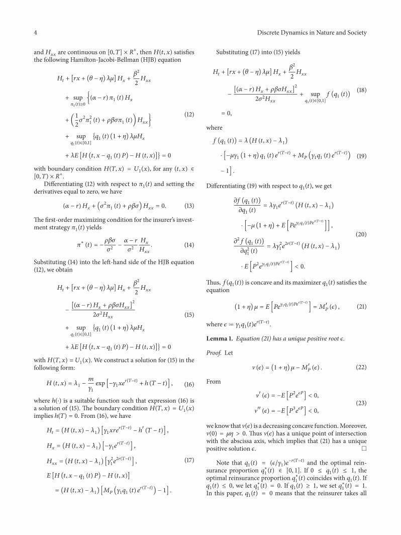
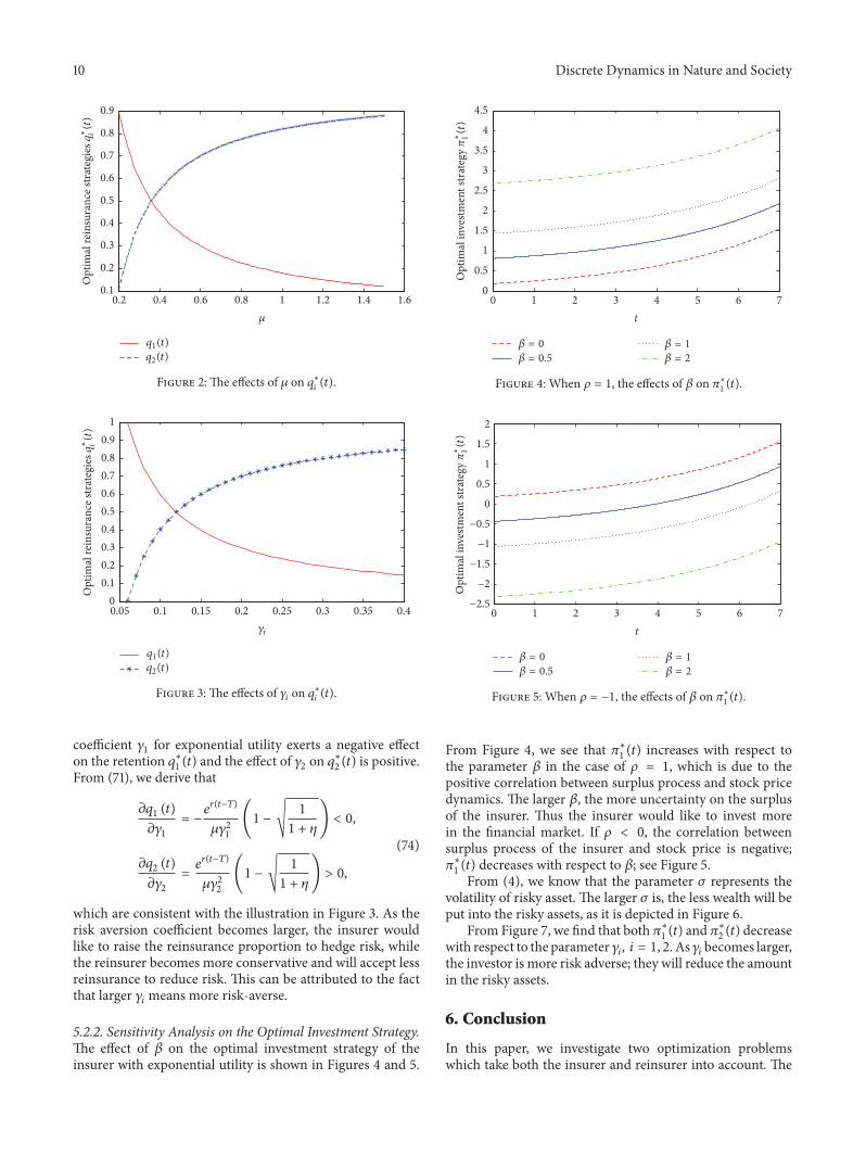
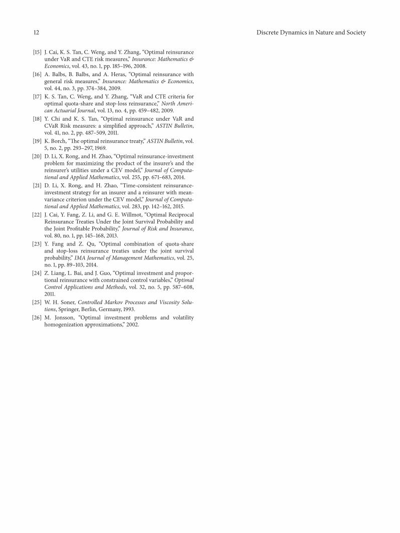

Hindawiwwwhindawicom Volume 2018
MathematicsJournal of
Hindawiwwwhindawicom Volume 2018
Mathematical Problems in Engineering
Applied MathematicsJournal of
Hindawiwwwhindawicom Volume 2018
Probability and StatisticsHindawiwwwhindawicom Volume 2018
Journal of
Hindawiwwwhindawicom Volume 2018
Mathematical PhysicsAdvances in
Complex AnalysisJournal of
Hindawiwwwhindawicom Volume 2018
OptimizationJournal of
Hindawiwwwhindawicom Volume 2018
Hindawiwwwhindawicom Volume 2018
Engineering Mathematics
International Journal of
Hindawiwwwhindawicom Volume 2018
Operations ResearchAdvances in
Journal of
Hindawiwwwhindawicom Volume 2018
Function SpacesAbstract and Applied AnalysisHindawiwwwhindawicom Volume 2018
International Journal of Mathematics and Mathematical Sciences
Hindawiwwwhindawicom Volume 2018
Hindawi Publishing Corporation httpwwwhindawicom Volume 2013Hindawiwwwhindawicom
The Scientific World Journal
Volume 2018
Hindawiwwwhindawicom Volume 2018Volume 2018
Numerical AnalysisNumerical AnalysisNumerical AnalysisNumerical AnalysisNumerical AnalysisNumerical AnalysisNumerical AnalysisNumerical AnalysisNumerical AnalysisNumerical AnalysisNumerical AnalysisNumerical AnalysisAdvances inAdvances in Discrete Dynamics in
Nature and SocietyHindawiwwwhindawicom Volume 2018
Hindawiwwwhindawicom
Dierential EquationsInternational Journal of
Volume 2018
Hindawiwwwhindawicom Volume 2018
Decision SciencesAdvances in
Hindawiwwwhindawicom Volume 2018
AnalysisInternational Journal of
Hindawiwwwhindawicom Volume 2018
Stochastic AnalysisInternational Journal of
Submit your manuscripts atwwwhindawicom