optimal real-time sampling rate assignment for wireless sensor...

Optimal Real-Time Sampling Rate Assignment forWireless Sensor Networks

Xue Liu, Qixin Wang, Wenbo He, Marco Caccamo and Lui Sha

University of Illinois at Urbana-Champaign

How to allocate computing and communication resources in a way that maximizes the efiective-ness of control and signal processing has been an important area of research. The characteristic ofa multi-hop Real-Time Wireless Sensor Network raises new challenges. First, the constraints aremore complicated and a new solution method is needed. Second, a distributed solution is neededto achieve scalability. This paper presents solutions to both of the new challenges. The flrst solu-tion to the optimal rate allocation is a centralized solution that can handle the more general formof constraints as compared with prior research. The second solution is a distributed version forlarge sensor networks using a pricing scheme. It is capable of incremental adjustment when utilityfunctions change. This paper also presents a new sensor device/network backbone architecture{ Real-time Independent CHannels (RICH), which can easily realize multi-hop real-time wirelesssensor networking.

Categories and Subject Descriptors: C.2.2 [Computer-communication Networks]: NetworkProtocols|Applications; C.3 [Special-purpose and Application-based Systems]: Real-timeand Embedded Systems|Applications

General Terms: Algorithms, Design, Performance, Experimentation

Additional Key Words and Phrases: Sensor Network, Real-Time Wireless Sensor Network, Opti-mization, Pricing, Distributed Algorithms

1. INTRODUCTION AND RELATED WORK

Real-Time Wireless Sensor Network (RTWSN) is expected to carry out variousapplications such as remote control or video/audio monitoring in ad hoc environ-ments. Instead of using conservative (lowest allowed) sampling/actuating rates(since sampling and actuating rate allocation are similar, unless explicitly denoted,\sampling rate" is used instead of \sampling/actuating rate" in the following), asampling rate allocation that maximizes global utility while maintaining real-time

Author’s address: Xue Liu, Qixin Wang, Wenbo He, Marco Caccamo and Lui Sha, Departmentof Computer Science, Univ. of Illinois at Urbana-Champaign, Urbana, IL 61801. Email: fxueliu,qwang4, wenbohe, mcaccamo, lrs [email protected] research is supported by (listed in alphabetical order) MURI N00014-01-0576, NSF ANI 02-21357, NSF CCR 02-09202, and ONR N00014-02-1-0102. The flrst two authors are also supportedby Saburo Muroga Fellowship and Vodafone Fellowship respectively.Part of this work has been published at 24th IEEE Real-Time Systems Symposium [Liu et al.2003].Permission to make digital/hard copy of all or part of this material without fee for personalor classroom use provided that the copies are not made or distributed for proflt or commercialadvantage, the ACM copyright/server notice, the title of the publication, and its date appear, andnotice is given that copying is by permission of the ACM, Inc. To copy otherwise, to republish,to post on servers, or to redistribute to lists requires prior speciflc permission and/or a fee.c° 2006 ACM 1529-3785/2006/0700-0001 $5.00

ACM Transactions on Sensor Networks, Vol. V, No. N, January 2006, Pages 1{34.

2 ¢schedulability is wanted.

Resource allocation has been studied in general for computing systems [Kuroseand Simha 1989; Waldspurger and Weihl 1994; Bolot et al. 1994]. Recently, theproblem of resource allocation and congestion control in network has been studiedtogether by Kelly and Low et al. [Kelly et al. 1998; Kelly 1997; Low and Lapsley1999]. However, these works do not consider real-time constraints, and thereforecannot be directly applied to real-time systems.

Stoica et al. [1996] have studied a proportional share resource allocation algo-rithm for real-time, time-shared system. The scheme is for single processor schedul-ing and is more focused on fairness of the scheduling algorithms rather than systemoptimality. Finding the optimal control rates subject to schedulability constraintswas flrst studied by Seto et al. [1996] and by Sha et al. [2000] for analog and digitalcontrollers respectively. An o†ine solution method is given based on Kuhn-Tuckercondition. However, the schedulability analysis is still for single processor. Ra-jkumar et al. [1997] investigated QoS-based Resource Allocation Model (Q-RAM),which is capable of handling complex multiple quality dimensions. But the solutioncan only be used with single constraint scenario. In the following works, Lee [1999]and Ghosh [2003] et al. studied the scenario under multiple constraints. However,the problem they studied is an integer programming problem, which is difierentfrom the model we will discuss in this paper. In [Lee et al. 1999], the integer pro-gramming problem is proven to be NP-Hard. Several sub-optimal algorithms areproposed. According to [Ghosh et al. 2003], the one that scales well is HierarchicalQ-RAM. However, that algorithm requires the division of multiple constraints intoindependent groups, which is impractical for multi-hop RTWSN.

RTWSN presents new challenges for real-time resource allocation. Routes in aRTWSN may interleave with each other. The sampling rate optimization must takeinto consideration the tra–c contention at each router. This makes the optimizationproblem harder than those studied before. We present an Interior Point Method(IPM) based solution to show how the optimal rates can be found e–ciently. On theother hand, though a centralized method is usually e–cient for small and moder-ately large RTWSNs, it may not scale well for very large RTWSNs, because controlmessages for optimization converge at the central node and create a bottleneck. Todynamically flnd the global optimum in a very large network, a distributed solutionis needed to generate balanced optimization control tra–c that avoids bottlenecks.In addition, the solution shall be incremental, so that when the utility functions ata few nodes change, updated optimum can be found with small cost.

To the best of our knowledge, works by Caccamo et al. [2002] are the flrst toprovide real-time support for multi-hop RTWSN. In [Caccamo et al. 2002], a cellularbase station layout is deployed as the backbone for the whole RTWSN, as shown inFig. 1. The base station network uses seven non-overlapping Radio Frequency (RF)bands. At the center of each cell, there is one base station, which also functions asa router. A router in a cell labeled i has a single transmitter that always transmitsat RF band i, and a single receiver that receives from one neighbor at a time(i.e. listens to one of the six neighbors’ RF bands at a time). All RF broadcastsare one-hop. The speciflc geographical layout makes each base station and its sixneighbors transmits with distinct RF bands, and any two base stations sending with

ACM Transactions on Sensor Networks, Vol. V, No. N, January 2006.

¢ 3

1

25 7

34

6

1

25 7

34

1

25 7

34

6

1

25 7

34

6

6

34

6

1

25 7

34

6 7

1

25 7

34

6

1

25

Fig. 1. A mixed FDMA-TDMA base station backbone layout

the same RF band are at least two cells apart. The inter-cell communication uses aglobally synchronized TDMA scheme. Speciflcally, all base stations’ receivers listento their northeast neighbors at time slot 1, listen to east neighbors at time slot2, so on and so forth. Therefore, the inter-base station communication is a mixedFDMA-TDMA scheme. More recently, based on the mixed FDMA-TDMA scheme,Giannecchini et al. [2004] provide an online suboptimal approximation algorithm(CoRAl) to dynamically reconflgure sensing rates of RTWSN. CoRAl runs fast butonly applies to exponential performance loss function. It is worth mentioning thatinside of each cell, there can be randomly distributed wireless slave sensors withmore constrained capabilities, which does the actual sensing and communicateswith the cell’s base station at other RF bands (which do not interfere with inter-base station communications). The intra-cell communication is not the focus ofthis paper, and therefore intra-cell sensors are not plotted in this paper’s flgures.

We adopt Caccamo et al. [2002]’s cellular base station backbone layout. In thispaper, we focus on the scenario that data °ows among backbone base stations areunicast °ows. More sophisticated routing topologies such as multicast and con-vergecast are beyond the scope of this paper1. Also, we assume routes are alreadydecided by given algorithms, for example SPIN [Heinzelman et al. 1999], GPSR[Karp and Kung 2000], GEAR [Xu et al. 2001], SPEED [He et al. 2003] or RumorRouting [Braginsky and Estrin 2002] etc.2; and the total data bandwidth of eachone-hop wireless link is adjusted so that the wireless medium is reliable enoughfor real-time communication (according to information theory and CDMA thoery

1Intra-cell communications between slave sensors and the base station are more often convergecast,but is not the focus of this paper.2A good survey of routing protocols in sensor networks is given in [Akkaya and Younis 2005]


4 ¢[Viterbi 1995] (also see Appendix A), if the worst case wireless medium condition isgiven, there is an upper bound on data bit throughput so that the data bit error ratecan be maintained below an upper bound). How to incorporate routing and toleratedevice failures and message drops into our sampling rate optimization are future re-search issues beyond the scope of this paper. According to information theory, theinter-base station bandwidth available is determined by wireless medium qualityand reception quality requirements, and is fundamentally irrelevant with speciflcmultiple access schemes, such as FDMA, TDMA or CDMA. The mixed FDMA-TDMA multiple access scheme proposed in Caccamo et al. [2002] provides poorer°exibility on bandwidth allocation adjustment, and the scheduling mechanism ismore complicated. Therefore, in this paper, we propose a mixed FDMA and DirectSequence Spread Spectrum CDMA (DSSS-CDMA)3 scheme called Real-time Inde-pendent CHannels (RICH), which provides better °exibility and whose real-timescheduling is easier to implement and analyze. A brief tutorial on DSSS-CDMA isprovided in Appendix A.

The major contributions of this paper are:

|Study and model the optimal rate assignment problem in RICH multi-hop RTWSNusing real-time schedulability analysis and non-linear optimization.

|Using the state-of-art methods in optimization, two solutions to the optimal rateassignment problem are given. One is in a centralized fashion using Interior PointMethod, the other is in a distributed fashion based on pricing scheme.

|Compare the trade-ofis between the centralized and distributed algorithms underdifierent situations.

The rest of the paper is organized as follows. Section 2 describes our proposedRICH architecture, which can easily support multi-hop real-time networking. Wealso give the real-time schedulability constraints analysis in this section. An exam-ple of RICH RTWSN is presented to show the practicability of RICH. In Section 3,we formulate the optimal QoS sampling rate assignment problem into a non-linearprogramming problem. Section 4 and 5 give centralized and distributed solutionfor optimal QoS sampling rate assignment respectively. In Section 6, we flrst com-pare the numerical solutions based on the example discussed in Section 2, discussin details the trade-ofis between the centralized and distributed solution. Then weanalyze the possible problems and solutions associated with both methods. Finally,conclusions and future work are discussed in Section 7.

2. SUPPORTING MULTI-HOP RTWSN

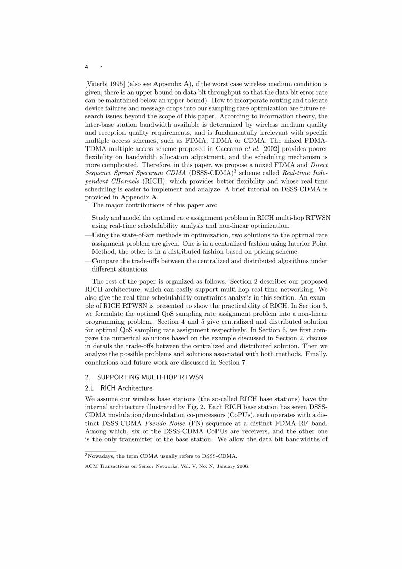
2.1 RICH Architecture

We assume our wireless base stations (the so-called RICH base stations) have theinternal architecture illustrated by Fig. 2. Each RICH base station has seven DSSS-CDMA modulation/demodulation co-processors (CoPUs), each operates with a dis-tinct DSSS-CDMA Pseudo Noise (PN) sequence at a distinct FDMA RF band.Among which, six of the DSSS-CDMA CoPUs are receivers, and the other oneis the only transmitter of the base station. We allow the data bit bandwidths of

3Nowadays, the term CDMA usually refers to DSSS-CDMA.


¢ 5

each DSSS-CDMA CoPU to be distinct. For the time being, suppose the singulartransmitter sends packets according to Earliest Deadline First (EDF) scheduling al-gorithm. A dedicated EDF scheduling queue is attached to it to bufier/schedule theoutgoing packets. In addition, a RICH base station also includes a sensing CoPU, oran intra-cell communication CoPU that gathers data from intra-cell slave sensors.The CPU interacts with each CoPU by periodical polling.

Sender EDF

Scheduling

QueueCPU

DSSS−CDMA

CoPU

(Sender)

Bit Reg

ReceivedDSSS−CDMA

(Receiver)

CoPU 2Bit Reg

ReceivedDSSS−CDMA

(Receiver)

CoPU 3Bit Reg

Received

DSSS−CDMA

(Receiver)

CoPU 6Bit Reg

ReceivedDSSS−CDMA

(Receiver)

CoPU 5Bit Reg

ReceivedDSSS−CDMA

(Receiver)

CoPU 4Bit Reg

Received

DSSS−CDMA

(Receiver)

CoPU 1

RF CoPU for

comm. with

slave

sensors.

Or local

sensing

CoPU.

intra−cell

Wireless Channel 1 Wireless Channel 2 Wireless Channel 3

Wireless Channel 4 Wireless Channel 5 Wireless Channel 6

Wireless Channel 7

Sending

Bit Reg

Fig. 2. Internal Architecture of a RICH Base Station

We adopt the cellular base station layout of Caccamo et al. [2002]’s (see Fig. 3),and maintain the seven RF band coloring of the cells. Meanwhile, we deploy forty-nine DSSS-CDMA PN sequences, denoted as A1; : : : ; A7, B1; : : : ; B7, C1; : : : ; C7,D1 : : : ; D7, E1; : : : ; E7, F 1; : : : ; F7, G1; : : :, and G7 respectively. In a cell labeledXY , the RICH base station transmitter deploys the XY th PN sequence for DSSS-CDMA modulation, and transmits at the Y th RF band. For example, the basestation in a cell labeled G7 transmits with the G7th DSSS-CDMA PN sequence atthe 7th RF band. The transmission range of every transmitter in our RICH RTWSNis one-hop. Each of the six receivers on a RICH base station listens to one of itsone-hop neighbor’s transmission. Take the RICH base station at a cell labeled A5for example, its six receivers listens to the 6; 7; 4; 1; 3; 2th RF band respectively, anddemodulates with DSSS-CDMA PN sequence A6; A7; A4; G1; F 3; F 2 respectively.

Under such design, the broadcast of a base station is simultaneously receivedby its six one-hop neighbors. The efiective receiver is designated by the broadcast


6 ¢

G1G6

G7G5 G2

G3G4

F1F6

F7F5 F2

F3F4

A1A6

A7A5 A2

A3A4

B1B6

B7B5 B2

B3B4C1C6

C7C5 C2

C3C4

D1D6

D7D5 D2

D3D4

E1E6

E7E5 E2

E3E4

G1G6

G7G5 G2

G3G4

F1F6

F7F5 F2

F3F4

A1A6

A7A5 A2

A3A4

B1B6

B7B5 B2

B3B4C1C6

C7C5 C2

C3C4

D1D6

D7D5 D2

D3D4

E1E6

E7E5 E2

E3E4

......

......

Fig. 3. The mixed FDMA-CDMA base station backbone layout

packet’s \destination" data segment. More importantly, because of the deploymentof DSSS-CDMA, any transmission can be carried out independently. For example,in Fig. 3, an F2 base station and an A6 base station can both send packets toan A5 base station (their common one-hop neighbor) at anytime. Furthermore,the schedule can be independently adjusted to be per base station speciflc. Forexample, the F 2 base station can dedicate 100% of its time sending to the A5base station; at the same time, the A6 base station can dedicate 1

3 of its time tothe A5 base station. There is no synchronization requirements between any pairof transmissions. Under TDMA, however, this is impossible. For example, F 2’ssending schedule must not overlap with A6’s. Such mutual exclusive relationshippropagates throughout the network, flnally all base stations’ broadcast schedulesare inter-locked, which complicates analysis and reconflguration.

Also, the layout guarantees two base stations transmiting with same DSSS-CDMA PN sequence (and therefore at the same RF band) are at least eight hopsaway. This implies that a base station does not have to be at the center of its cell.

2.2 Schedulability Analysis of RICH RTWSN

The broadcast of a RICH base station is overheard by all its six neighbor basestations. Usually, the wireless medium to the six neighbors are irregular [Zhouet al. 2004; Zhao and Govindan 2003]. According to DSSS-CDMA theory (seeAppendix A), given RF band, worst case wireless medium conditions and maximumacceptable bit error rate, the upper bound of data bit bandwidth is determined,


¢ 7

which we call afiordable bandwidth. Suppose for a RICH base station X, because ofthe irregularity of wireless medium, the afiordable bandwidths to its six neighboringRICH base stations are B1, B2, : : :, B6. We set the transmission data bit bandwidthof X to be B = minfB1; B2; : : : ; B6g. Therefore the broadcast of X is reliablyreceived by all its six neighbors, i.e. the bit error rate of one-hop transmission isalways below the maximum acceptable bound. In another word, B models factorssuch as the impact of radio irregularity on the wireless medium.

For a RICH base station, the real-time scheduling is carried out in the EDFscheduling queue attached to its singular transmitter. Let T be the set of all routesthat go through it. For a route ¿ 2 T , suppose it has a sampling/reporting rateof f¿ , and each report is a packet of length l¿ . The corresponding transmissiontime of the packet is therefore c¿ = l¿ =B. When there are multiple contendingroutes through one RICH base station, the transmitter should be regarded as anon-preemptive resource. Because once a packet starts transmitting, it cannotbe preempted until completely transmitted. Hereby, the real-time scheduler of aRICH base station’s EDF queue should be non-preemptive EDF scheduler to ensureboth the EDF behavior and non-preemptive usage of the broadcast link. Undersuch scheduling, a packet (job) can be blocked by at the most one other packet.Therefore we can apply the well-known schedulability bound for the non-preemptiveEDF scheduler as follows [Buttazzo 1997]:

X

¿2Tc¿ f¿ + Cjfj • 1, for each j 2 T ; (1)

where Cj is the maximum blocking time for sending a packet of route j.

Cj = maxf¿2T and ¿ 6=jg

fc¿ g

= maxf¿2T and ¿ 6=jg

‰l¿

B

¾

= maxf¿2T and ¿ 6=jg

fl¿ gB

:

Therefore (1) is transformed into:

X

¿2T

l¿

Bf¿ +

Lj

Bfj • 1, for each j 2 T ; (2)

where Lj = maxf¿2T and ¿ 6=jgfl¿ g.

Multiply both sides of Eq. (2) with broadcast link bandwidth B, we getX

¿2Tl¿ f¿ + Ljfj • B, for each j 2 T : (3)

Besides of being a router, a RICH base station can also simultaneously functionas the source end of a route. The data are either from the base station’s localsensing CoPU or by gathering intra-cell slave sensors’ readings. Either way, thebase station can be regarded as the virtual singular source end sensor for the route,and its sampling rate is upper bounded, creating the following constraint (for the


8 ¢time being, we assume each base station can be the source end of at the most oneroute):

fj • fmaxj ; (4)

where fj is the sampling rate of route j, and fmaxj is the maximum afiordable

sampling rate at the route’s source end base station. 4 Hereby, by analyzing eachbase station of the RICH RTWSN according to inequality set (3) and each routeaccording to inequality (4), we can derive a set of linear inequalities, which isthe su–cient real-time schedulability constraints for RICH RTWSN sampling rateassignment. We can summarize them into the following form:

(Af • W

f • fmax;(5)

where f = (f1; f2; : : : ; fN )T is the vector of sampling rates assigned to each ofthe N routes. fmax = (fmax

1 ; fmax2 ; : : : ; fmax

N )T is the maximum sampling rate forthe N end point sensors (see (4)). Matrix A and vector W are obtained by basestation-wise analysis according to (3), which re°ect the speciflc routing topology ofthe RICH RTWSN. Suppose these schedulability analysis generate M inequalitiesin total, then A 2 RM£N , W 2 RM£1.

Besides the constraints from real-time schedulability, there are often applicationspeciflc minimum sampling/reporting rate requirements. These extra requirementscan be written as:

f ‚ fmin = (fmin1 ; : : : ; fmin

N )T: (6)

Inequality set (5) and (6) constitute a complete set of real-time schedulabilityconstraints for RICH RTWSN sampling rate allocation. An example is given asfollows:

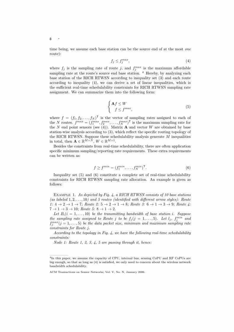
Example 1. As depicted by Fig. 4, a RICH RTWSN consists of 10 base stations(as labeled 1; 2; : : : ; 10) and 5 routes (identifled with difierent arrow styles): Route1: 4 ! 2 ! 1 ! 7; Route 2: 5 ! 2 ! 1 ! 8; Route 3: 6 ! 1 ! 3 ! 9; Route 4:7 ! 1 ! 3 ! 10; Route 5: 8 ! 1 ! 2.

Let Bi(i = 1; : : : ; 10) be the transmitting bandwidth of base station i. Supposethe sampling rate assigned to Route j to be fj(j = 1; : : : ; 5). Let lj, fmin

j andfmax

j (j = 1; : : : ; 5) be the data packet size, minimum and maximum sampling rateconstraints for Route j.

According to the topology in Fig. 4, we have the following real-time schedulabilityconstraints:

Node 1: Route 1, 2, 3, 4, 5 are passing through it, hence:

4In this paper, we assume the capacity of CPU, internal bus, sensing CoPU and RF CoPUs arebig enough, so that as long as (4) is satisfled, we only need to concern about the wireless networkbandwidth schedulability.


¢ 9

1 8

6

3

24

5

9

10

7

1Route

2345

Fig. 4. A RICH RTWSN Schedulability Analysis Example

(l1f1 + l2f2 + l3f3 + l4f4 + l5f5) + maxfl2; l3; l4; l5gf1 • B1





Node 2: Route 1, 2 are passing through it, hence:

(l1f1 + l2f2) + l2f1 • B2

(l1f1 + l2f2) + l1f2 • B2

As the destination end for Route 5, there are no constraints (the correspondingconstraints are analyzed at base station 1, Route 5’s last sending hop).

Node 3: Route 3,4 are passing through it, hence:

(l3f3 + l4f4) + l4f3 • B3

(l3f3 + l4f4) + l3f4 • B3

Node 4: As a base station along Route 1, we have l1f1 • B4.Node 5: As a base station along Route 2, we have l2f2 • B5.Node 6: As a base station along Route 3, we have l3f3 • B6.Node 7: As a base station along Route 4, we have l4f4 • B7. As the destination

end for Route 1, there are no constraints (the corresponding constraints are analyzedat base station 1, Route 1’s last sending hop).

Node 8: As a base station along Route 5, we have l5f5 • B8. As the destinationend for Route 2, there are no constraints (the corresponding constraints are analyzedat base station 1, Route 2’s last sending hop).

Node 9 and Node 10: As purely destination end for routes, there are no con-straints (corresponding constraints are analyzed at the corresponding routes’ lastsending hops).


10 ¢8>>>>>>>>>>>>>>>>>>>>>>>>>>>>><>>>>>>>>>>>>>>>>>>>>>>>>>>>>>:

A =

2666666666666666666666664

l1 + maxfl2; l3; l4; l5g l2 l3 l4 l5l1 l2 + maxfl1; l3; l4; l5g l3 l4 l5l1 l2 l3 + maxfl1; l2; l4; l5g l4 l5l1 l2 l3 l4 + maxfl1; l2; l3; l5g l5l1 l2 l3 l4 l5 + maxfl1; l2; l3; l4g

l1 + l2 l2 0 0 0l1 l1 + l2 0 0 00 0 l3 + l4 l4 00 0 l3 l3 + l4 0l1 0 0 0 00 l2 0 0 00 0 l3 0 00 0 0 l4 00 0 0 0 l5

3777777777777777777777775

f = (f1; f2; f3; f4; f5)T

W = (B1; B1; B1; B1; B1; B2; B2; B3; B3; B4; B5; B6; B7; B8)T

(7)

In addition to all above, because of the minimum sampling rate constraints, wehave: fj ‚ fmin

j , where (j = 1; : : : ; 5). The complete rate allocation constraints are

hereby: Af • W , f • (fmax1 ; : : : ; fmax

5 )T and f ‚ (fmin1 ; : : : ; fmin

5 )T, which aredetailed by (7).

Suppose the numerical values of parameters are as shown in Table I, then thecomplete rate allocation constraints are transformed into (8).

Table I. Parameter Values for Example 1

Node Bandwidth(Bi Mbps) Max Sampling Capability(fmax Hz)

1 1.0 -

2 0.6 -

3 0.4 -

4 0.25 (fmax1 = )30

5 0.25 (fmax2 = )25

6 0.25 (fmax3 = )30

7 0.2 (fmax4 = )40

8 0.15 (fmax5 = )30

Route Required MinFreq. (fmin

j

Hz)

AfiordableMax Freq.(fmax

j Hz)

Report PacketSize (lj Mbit)

1 11 30 0.01

2 2.5 25 0.015

3 5 30 0.02

4 1 40 0.025

5 2 30 0.03

3. OPTIMIZING QOS IN WSN WITH REAL-TIME CONSTRAINTS | MATH MOD-ELING

In this section, we model the optimal sampling rate allocation problem as an non-linear convex optimization problem, using constraints set (5)(6) from the previous


¢ 11

8>>>>>>>>>>>>>>>>>>>>>>><>>>>>>>>>>>>>>>>>>>>>>>:

Af =

2666666666666666666664

:04 :015 :02 :025 :03:01 :045 :02 :025 :03:01 :015 :05 :025 :03:01 :015 :02 :055 :03:01 :015 :02 :025 :055

:025 :015 0 0 0:01 :025 0 0 00 0 :045 :025 00 0 :02 :045 0

:01 0 0 0 00 :015 0 0 00 0 :02 0 00 0 0 :025 00 0 0 0 :03

3777777777777777777775

26664

f1

f2

f3

f4

f5

37775 • W =

2666666666666666666664

1:01:01:01:01:0:6:6:4:4

:25:25:25:2

:15

3777777777777777777775

;

f • fmax

= (30; 25; 30; 40; 30)T

, and f ‚ fmin

= (11; 2:5; 5; 1; 2)T

:

(8)

section.

3.1 Utility Loss Index

The base station at the source end of a route periodically samples and reportssensor readings. Let the sampling/reporting rate (or \frequency") for the jth routebe fj . For most applications, the higher the sampling/reporting rate fj , the higheris the QoS. For example, for control applications, the faster the sampling rate, thebetter the control performance [Seto et al. 1996]. Ideally, the best performanceis achieved if the sampling rate is approaching 1, i.e. continuous sampling. Inpractice, this is not achievable, so we use Utility Loss Index (ULI) function tocapture the performance loss at a discrete sampling rate f compared to continuoussampling. For control applications, Seto et al. [1996] shows the ULI is in thefollowing form:

Uj(fj) = !jfije¡fljfj ; (9)

where fj is the sampling rate for task j (i.e. route j), !j , fij and flj are applicationspeciflc constraints. The values of !j , fij and flj can be determined through datafltting using real-world measurements. In this paper, the form of ULI function isgeneralized to be any strictly decreasing difierentiable convex function with regardto rate f .

3.2 Mathematical Formulation

Assume each individual ULI function Uj(fj) is strictly decreasing difierentiable andconvex. Suppose ULIs are additive, the system’s overall ULI is thereby the sumof the ULIs of all individual routes:

PNj=1 Uj(fj). The performance optimization

problem becomes:

min(f1;:::;fN )

PNj=1 Uj(fj) (10)

s.t.: Af • W (11)

f • fmax (12)

f ‚ fmin (13)

where A is a constraint matrix with dimension M £ N . M is dependent upon the


12 ¢routing topology of the RTWSN, and N is the number of total routes. We call thisproblem Multiple Constraints Optimization Problem (MCOP) in contrast to Setoet al. [1996]’s Single Constraint Optimization Problem (SCOP), and we denote theformer as MCOP (U; A; W ).5

The feasible set of MCOP is compact and convex and Uj(fj) is difierentiable andconvex, therefore MCOP has optimal solutions [Bertsekas 1995]. Furthermore, ifUj(fj) is strictly convex, the optimal solution is unique [Bertsekas 1995].

When M = 1 and there is no constraint set (12), then the ULIs are in thenegative exponential form, and MCOP (U; A; W ) becomes SCOP as follows [Setoet al. 1996]:

min(f1;:::;fN )

PNj=1 Uj(fj) =

NX

j=1

!jfije¡fljfj (14)

s.t.: Af • W (15)

f ‚ fmin = (fmin1 ; : : : ; fmin

N )T (16)

where W is the bandwidth (utilization) constraints, and A 2 R1£N ; f 2 RN£1; W 2R.

Based on Kuhn-Tucker condition, Seto et al. [1996] provides an algorithm tosolve SCOP problem analytically. MCOP is a generalization of SCOP. We shallshow that the approach for deriving an analytical solution to SCOP is not viablefor solving MCOP. To this end, we flrst prove that the optimal solution f⁄ ofMCOP will make at least one of the constraints in constraint sets (11) and (12)becomes equality constraint and show why it is not viable to tackle the MCOP inan analytical fashion similar to [Seto et al. 1996]. In MCOP (U; A; W ), constraintset (11) and (12) can be combined as:

A0f • W 0;

where A0 =

•AI

‚

(M+N)£N

, W 0 =

•W

fmax

‚

(M+N)£1

(17)

Theorem 3.1. MCOP’s optimal solution f⁄ must ensure that at least one ofthe (M + N) constraints A0

if⁄ • W 0

i ; i = 1; : : : ; (M + N) reaches equality. i.e.,9i 2 f1; : : : ; M + Ng such that A0

if⁄ = W 0

i . Here A0i is the ith row of A0.

Proof. Please refer to Appendix B for the proof.

Though we know for the optimal rate assignment f⁄ there is at least one i suchthat A0

if⁄ = W 0

i , we do not know explicitly which constraints reach equality. Thismakes the Kuhn-Tucker based solution method not applicable. In contrast, theproblem discussed in [Seto et al. 1996], which is a SCOP (M = 1), is much easierbecause there is only one non-trivial constraint A1f⁄ • W1, and it is exactly thisconstraint that should reach equality. In addition to [Seto et al. 1996], Rajkumar

5Notation used in [Kelly et al. 1998].


¢ 13

et al. [1997] proposed a numerical solution. But that solution is also for singleconstraint scenario. In their more recent works, Lee [1999] and Ghosh [2003] etal. studied the scenario under multiple constraints. However, the problem theystudied is an integer programming problem, which is difierent from the model wewill discuss in this paper. In [Lee et al. 1999], the integer programming problem isproven to be NP-Hard. Several sub-optimal algorithms are proposed. According to[Ghosh et al. 2003], the one that scales well is Hierarchical Q-RAM. However, thatalgorithm requires the division of multiple constraints into independent groups,which is impractical for multi-hop RTWSN (see Section 6.5). Fortunately, as willbecome clear later, MCOP can be solved with the state-of-art Interior Point Meth-ods [Nesterov and Nemirovsky 1994; Ye 1997a] and Internet pricing schemes [Lowand Lapsley 1999; Kelly et al. 1998; Kelly 1997].

4. CENTRALIZED SOLUTION METHOD FOR MCOP

In this section, we apply Interior Point Method (IPM) to solve the MCOP problemfor RTWSN.

Deflnition 4.1. A Constrained Optimization Problem is expressed as minff(x) :x 2 Q µ Rng, where the constraint set Q is deflned by multiple equalities andinequalities: Q = fx : h(x) = 0; g(x) • 0g, where h : Rn ! Rp; g : Rn ! Rq.

Deflnition 4.2. A Convex Optimization (CO) problem is a constrained optimiza-tion problem whose objective function f(x) is continuous and convex, and whoseconstraint set Q is compact (i.e. closed and bounded) and convex.

It’s easy to see that an MCOP is a constrained convex optimization problem withlinear constraints. For solving a convex optimization problem, the major di–cultiescome from the multiple inequality constraints. Closed form solutions are generallyunavailable. However, IPMs [Nesterov and Nemirovsky 1994; Ye 1997a] can solvelinear constraint convex optimization problems numerically. IPM is a numericalmethod that iterates in the interior of the solution space deflned by constraint set Qto flnd the optimal solution. IPMs can be further divided into two sub-categories:primal methods and primal-dual methods. Primal-dual methods try to solve theprimal and dual optimization problems [Luenberger 1984] together. In practice, theprimal-dual methods are more e–cient. The advantages of interior-point methodbased numerical solution includes: (1) E–cient. IPMs give the correct solutionvery fast; (2) Multi-hop application scenarios: The objective function needs not tobe conflned as exponential form as in paper [Seto et al. 1996], but can be generalstrictly decreasing difierentiable convex functions.

To solve the MCOP problem, we use optimization library COPL LC [Ye 1997b].It is easy to transform our MCOP problem to the form used by COPL LC. Thetransformation method can be found in Appendix C. To implement the IPM basedcentralized solution, the whole RICH RTWSN elects a central computing node C,which gathers ULI and constraints information from all the network, carries outthe optimization algorithm, and returns the flnal results.


14 ¢5. DISTRIBUTED ALGORITHMS FOR OPTIMAL RATE ASSIGNMENT

However, a direct application of IPM results in a centralized solution that requirescollecting data from each node. This will create a tra–c bottleneck around thecentral computing node (detailed discussion is in Section 6.5). To overcome thebottleneck problem, we give a distributed algorithm for solving the MCOP. Thedistributed algorithm let routers and routes’ end point nodes collaborate to flndthe optimal rates. The algorithm is based on the recent researches of Internetpricing schemes [Low and Lapsley 1999; Kelly et al. 1998; Kelly 1997], especially[Low and Lapsley 1999].

The main idea is to impose a price on each constraint in (11)»(13). Each routewill accumulate its relevant constraints’ prices and solve a local optimization prob-lem based on its own ULI function. The result is the next proposed sampling ratefor the route (to simplify, we call it rate proposal in the following). The rate pro-posal is then delivered to each of the route’s routers, where each of the route’srelevant constraint updates (imagine each constraint as an active agent) its price(called constraint price) accordingly. This procedure works in an iterative manneruntil it converges.

The distributed algorithms has two main attributes:

(1) It converges to the optimal rates of MCOP (Theorem 5.1).

(2) Each route’s computation is only based on local information.

Notations used in the Distributed Algorithm:

s. is the algorithm’s iteration step, s = 0; 1; : : :.

p(s). is the updated constraint price vector for each constraint i; i 2 f1; : : : ; Mgat iteration step s. p(s) = (p1(s); : : : ; pM (s)).

f(s). is the updated rate proposal vector for each route j; j 2 f1; : : : ; Ng atiteration step s. f(s) = (f1(s); : : : ; fN (s))T.

The Distributed Algorithm:The distributed algorithm is made up of iterations. Each iteration consists of

two consecutive steps: the Constraint Algorithm, and the Route Algorithm.At the very beginning of the distributed algorithm, set f(0) = fmin, and p(0) ‚ 0.

1) Constraint AlgorithmDuring iteration s = 1; 2; : : :, for each constraint i(i = 1; : : : ; M):

C1. Receives rate proposal fj(s) from each relevant route j. Route j and constrainti are relevant if Aij 6= 0.

C2. Computes a new constraint price for itself using the following price updateequation:

pi(s + 1) = [pi(s) + °(f i(s) ¡ Wi)]+ (18)

Here f i(s) = Aif(s), and Ai is the ith row of A. Function [†]+ is deflned as[x]+ = maxfx; 0g, where x is a real number.

C3. Delivers new price pi(s + 1) to all routes which are relevant to constraint i.


¢ 15

2) Route AlgorithmDuring iteration s = 1; 2; : : :, for each route j(j = 1; : : : ; N):

R1. Receives from the network the sum of all the constraints’ prices pj(s) imposedon this route:

pj(t) =

MX

i=1

pi(s)Aij (19)

R2. Update the route’s rate proposal fj(s + 1) for the next iteration according tolocal optimization of:

min Uj(fj) + fjpj(s)

s.t.: fminj • fj • fmax

j

i.e. fj(s + 1) = arg minfmin

j •fj•fmaxj

(Uj(fj) + fjpj(s)) (20)

The iteration of Constraint and Route Algorithms stops until the predeflnedconvergence criterion is reached. For example, when both of the following twocriteria are met.

kf(s) ¡ f(s ¡ 1)kn • "f ; (21)

kq(s) ¡ q(s ¡ 1)kn • "q; (22)

where f(s) = (f1(s); f2(s); : : : ; fN (s))T, q(s) = (p1(s); p2(s); : : : ; pN (s))T. "f > 0and "p > 0 are su–ciently small real numbers. kvkn denotes the nth-norm ofvector v = (v1; : : : ; vk). If n = 1, kvk1 = max(vi); i 2 f1; : : : ; kg. If n 2 Z+, then

kvkn = (Pk

i=1 vni )

1n .

Now we prove the convergence and correctness of the above iterative algorithm.This is summarized in Theorem 5.1. First, we give the assumptions and notationsto be used.

Assumptions:

A1. The feasibility condition holds for each constraint i(i = 1; : : : ; M), such thatPNj=1 Aijfmin

j • Wi.

A2. For each route j, on the interval Ij = [fminj ; fmax

j ], the utility function Uj isstrictly decreasing, strictly convex, and twice continuously difierentiable.

A3. The curvatures of Uj for each route satisfles the following condition on Ij =[fmin

j ; fmaxj ], 9„fij , s.t. U 00

j (fj) ‚ 1„fij

> 0, for all fj 2 Ij .

Notations Used in Theorem 5.1:¢ L(j) =

PMi=1 Aij . It is the column sum of A;

¢ „L = maxj=1;:::;N fjL(j)jg, which is the maximum absolute value of column sumof A;


16 ¢¢ S(i) =

PNj=1 Aij . It is the row sum of A;

¢ „S = maxi=1;:::;M fjS(i)jg, which is the maximum absolute value of row sum of A;

¢ „fi = maxj=1;:::;N f„fijg. i.e. „fi is the upper bound on 1U 00

j (fj) ; j = 1; : : : ; N .

Theorem 5.1. Suppose assumptions A1 » A3 hold and the step size ° satisfy0 < ° < 2=(„fi„L „S). Then starting from any initial rates fmin • f(0) • fmax

and prices p(0) ‚ 0, the sequence f(f(s); p(s))g generated by the above distributedalgorithm will converge to a accumulation point (f⁄; p⁄), and f⁄ is the solution ofMCOP (U; A; W ).

Proof. See Appendix D.

6. EVALUATION

In this section, we shall present the simulation results and discuss the tradeofisbetween centralized algorithm and distributed algorithm, showing which is moreappropriate in what situations. We also show that distributed algorithm has thedesirable incremental adjustment property.

6.1 Implementation

First let us look at the real-world feasibility of RICH architecture. Real-world DSSSChip-Sets consists of multiple parallel independent transmitters and receivers are al-ready available. For example, the QualComm CSM2000 chipset [Qualcomm 2004a],originally designed for low-cost lightweight cellular base stations, supports eightparallel users, which is enough for the seven-transceiver RICH architecture. Higherperformance chipsets can be QualComm CSM5000 [Qualcomm 2004b], CSM5500[Qualcomm 2004c] etc., which can be easily reconflgured to build RICH base sta-tions, providing no less than 1:8Mbps data bandwidth for each of the seven trans-ceivers. The sizes and power consumption of these chip sets are also satisfactorillysmall. For example, a CSM5500 chip complies with BGA560 packaging, which is35 £ 35 £ 2:5mm in dimension; and is of 3 » 3:6volt I/O voltage and 1:8volt corevoltage.

Based on the above real-world parameters, we carry out simulation using J-Sim[DRCL 2004]. The centralized algorithm is straightforward. To simulate the distrib-uted algorithm, we need to devise a network protocol that matches the algorithmdescribed in Section 5, which is as following:

Network Protocol for Distributed Algorithm:The protocol is carried out in iterations, each iteration s consists of two steps:

Step 1 Each constraint’s price is updated by the router that creates that constraintbased on (18). Next, each of these updated prices must be propagated toall the relevant routes. To do that, each route’s source end sends an emptypacket toward the destination end. The packet’s payload is just one °oating-point number (i.e. 4 bytes), dedicated to carry the total price pj(s), where jrefers to the jth route. As this packet travels toward the destination along theroute, on each hop, it will accumulate onto pj(s) all relevant constraints’ prices


¢ 17

maintained by the local router. When the packet reaches the destination end,the total price pj(s) is obtained.

Step 2 After Step 1, each route’s destination end carries out the route algorithm(20) to update the sampling rate proposal. Then the destination end sendsanother packet towards the source end, to notify every router along this routeabout the updated sampling rate proposal. This packet’s payload is also justone °oating-point number (i.e. 4 bytes), which is enough to carry the updatedsampling rate proposal.

If the payload of the control tra–c is piggybacked to the data tra–c, it will adda 4 bytes overload. If the control tra–c is sent separately from the data tra–c,it can be encoded into a 16 byte packet. Within this 16 byte packet, 4 bytes arethe control payload, 4 bytes are for source address, and 4 bytes are for destinationaddress, and the remaining 4 bytes are for other purposes such as checksum etc. Inthe following discussions, we discuss the separate control message scheme, that is,the distributed algorithm incurs a 16 byte packet in Step 1 and Step 2 respectivelyfor each route.

For distributed algorithm, we also assume all the involved routes of the RTWSNare coarse-grain synchronized in the sense that in each iteration, all the routes flnishStep 1 and then move on to Step 2; and when all the routes flnish Step 2, theymove on to the next iteration. This can be achieved, e.g., by synchronizing all thenodes and start each step at time kTstep, where k 2 Z and Tstep is the empiricalupper bound of end-to-end packet travel time along the network diameter, assumingthere is a specifled upper bound on network diameter. The GPS System [Getting1993] can already provide global time synchronization with an accuracy of within0:25msec [Exit Consulting 2004], which is enough for our application. For example,in our simulation setup, a synchronization granularity of 2msec is enough for thetestbed.

6.2 Numerical Example of Centralized and Distributed Algorithm

First both the centralized and distributed algorithm are applied to the scenariodiscussed in Example 1 of Section 2.2. The setup involves 5 routes. The ULIfunction for each route j is in the form of !jfije¡fljfj , so the MCOP (U; A; W )’s

total ULI (i.e. the objective function) is:P5

j=1 Uj(fj) =P5

j=1 !jfije¡fljfj , withparameters shown in Table II. These parameters are taken from those reportedin [Sha et al. 2000]. Constraints are listed in equation (8).

Table II. Parameters for ULI in Example 1

Route fij flj !j

1 0.66 0.3 1

2 0.66 1.0 2

3 0.66 0.5 3

4 0.66 0.7 4

5 0.66 0.3 5


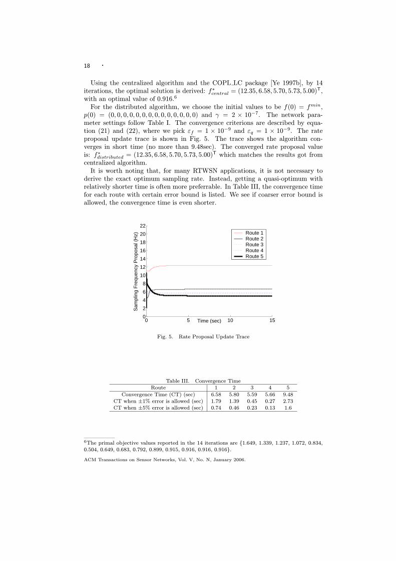
18 ¢Using the centralized algorithm and the COPL LC package [Ye 1997b], by 14

iterations, the optimal solution is derived: f⁄central = (12:35; 6:58; 5:70; 5:73; 5:00)T,

with an optimal value of 0.916.6

For the distributed algorithm, we choose the initial values to be f(0) = fmin,p(0) = (0; 0; 0; 0; 0; 0; 0; 0; 0; 0; 0; 0; 0; 0) and ° = 2 £ 10¡7. The network para-meter settings follow Table I. The convergence criterions are described by equa-tion (21) and (22), where we pick "f = 1 £ 10¡9 and "q = 1 £ 10¡9. The rateproposal update trace is shown in Fig. 5. The trace shows the algorithm con-verges in short time (no more than 9:48sec). The converged rate proposal valueis: f⁄

distributed = (12:35; 6:58; 5:70; 5:73; 5:00)T which matches the results got fromcentralized algorithm.

It is worth noting that, for many RTWSN applications, it is not necessary toderive the exact optimum sampling rate. Instead, getting a quasi-optimum withrelatively shorter time is often more preferrable. In Table III, the convergence timefor each route with certain error bound is listed. We see if coarser error bound isallowed, the convergence time is even shorter.

0 5 10 150

2

4

6

8

10

12

14

16

18

20

22

Time (sec)

Sam

plin

g F

requ

ency

Pro

posa

l (H

z) Route 1Route 2Route 3Route 4Route 5

Fig. 5. Rate Proposal Update Trace

Table III. Convergence TimeRoute 1 2 3 4 5

Convergence Time (CT) (sec) 6.58 5.80 5.59 5.66 9.48CT when §1% error is allowed (sec) 1.79 1.39 0.45 0.27 2.73CT when §5% error is allowed (sec) 0.74 0.46 0.23 0.13 1.6

6The primal objective values reported in the 14 iterations are f1.649, 1.339, 1.237, 1.072, 0.834,0.504, 0.649, 0.683, 0.792, 0.899, 0.915, 0.916, 0.916, 0.916g.


¢ 19

6.3 Monte Carlo Simulation on Convergence Speed

In order to give a feeling of how fast the distributed algorithm converges, thefollowing Monte Carlo simulation is carried out:

Rate error of route j at the sth iteration of distributed algorithm is deflnedas: e fj(s) = jfj(s) ¡ f⁄

j j, where fj(s) is the rate proposal for route j at the sthiteration; f⁄

j is the optimal sampling rate for this route.We still use the testbed depicted by Example 1. But in each trial of the Monte

Carlo, a difierent ULI function for each route is picked by setting the coe–cients of!j , fij and flj randomly. Then the distributed algorithm is carried out. The rateerror for iteration s = 1; : : : ; 500 is traced. Eight hundred trials are run. For eachroute, the eight hundred rate error traces are averaged and plotted in Fig. 6.

0 50 100 150 200 250 300 350 400 450 5000

1

2

3

4

5

6

7

Iteration steps

Err

or to

Opt

imal

Fre

quen

cy (

Hz)

Route 1Route 2Route 3Route 4Route 5

Fig. 6. Trace of error between proposed and optimal rates. Empirically, in 100 iterations, theproposed rates converge to a satisfactory range around the optimum.

According to Fig. 6, the rate error converges in a negative exponential form.Empirically, in 100 iterations the distributed algorithm reaches a satisfactory quasi-optimum.

It is worth noting that by exploiting the \incremental adjustment" propertydiscussed in Section 6.4, the distributed algorithm can converge even faster.

6.4 Incremental Adjustment Property of Distributed Algorithm

In real-world, there are often times that ULI functions and constraint set change dy-namically. These changes transform the original optimization problem MCOP (U; A; W )into a new optimization problem MCOP (U 0; A0; W 0), hence the optimal samplingrate f⁄ has to be re-calculated. If distributed algorithm is used, new iterations canbe carried out from the existing optimum (f⁄; p⁄), so as to reach the new optimum(f 0⁄; p0⁄) faster. We call this \incremental adjustment property". An example isgiven as follows:

Continue with the MCOP (U; A; W ) simulation example in Section 6.2. Supposeat time 15sec, the ULI coe–cients switch from old value set (see Table II) to the new


20 ¢value set depicted in Table IV. Fig. 7 and Table V shows the comparison betweenincremental and non-incremental adjustment schemes: the incremental adjustmentscheme starts with MCOP (U; A; W )’s optimum sampling rate and its correspond-ing price vector (f⁄; p⁄); the non-incremental adjustment scheme starts with aconstant tuple (f0; p0), where f0 = fmin and p0 = (0; 0; 0; 0; 0; 0; 0; 0; 0; 0; 0; 0; 0; 0).All other settings of the testbed are the same as those for Section 6.2, Under in-cremental adjustment scheme, in about 10:30sec, the rate proposal converges tothe new optimum f 0⁄. In contrast, if start from (f0; p0), the convergence to newoptimum f 0⁄ is much slower, taking 12:67sec.

Furthermore, if quasi-optimum is allowed, the new solutions can be derived faster.The convergence time costs are listed in Table V. The incremental adjustmentscheme still runs faster than the non-incremental version.

Table IV. New MCOP (U 0; A0; W 0) Parameters

Route fij flj !j

1 0.33 0.3 4

2 0.22 0.2 3

3 1.32 0.5 2

4 1.98 0.7 1

5 0.66 0.3 6

Table V. Convergence Time of MCOP (U 0; A0; W 0)Route 1 2 3 4 5

starts with Convergence Time (CT) (sec) 8.67 7.68 6.98 7.32 10.30(f⁄; p⁄) CT when §1% error is allowed (sec) 0.01 1.13 0.25 0.07 1.24

CT when §5% error is allowed (sec) 0.01 0.05 0.03 0.02 0.15

starts with Convergence Time (CT) (sec) 11.04 10.05 9.35 9.69 12.67(f0; p0) CT when §1% error is allowed (sec) 0.002 3.51 1.25 1.61 3.61

CT when §5% error is allowed (sec) 0.002 1.93 0.03 0.39 2.01

6.5 Control Tra–c and Scalability Analysis for Distributed and Centralized Algorithm

In this section, the control tra–c for both distributed and centralized algorithmsare analyzed. The centralized algorithm is e–cient even when the network is mod-erately large. However, when the network continues to scale up, the centralized al-gorithm would flnally reach its bottleneck. In contrast, under certain assumptions,the distributed algorithm provides better scalability, though it may be ine–cientfor smaller networks.

Control Tra–c Analysis for Distributed Algorithm:

Let N be the set of all base stations in a RICH RTWSN. Let `disi be the ac-

cumulated control tra–c (in bytes) passing through base station i(i 2 N ) underthe distributed algorithm. Let 'dis be the maximum accumulated control tra–c (inbytes) passing through any of the base stations, i.e. 'dis = maxi2N f`dis

i g.


¢ 21

15 20 25 300

2

4

6

8

10

12

14

16

18

20

22

Time (sec)

Sam

plin

g F

requ

ency

Pro

posa

l (H


(a) Based on MCOP (U; A; W )’s solution (f⁄; p⁄)

15 20 25 300

2

4

6

8

10

12

14

16

18

20

22

Time (sec)

Sam

plin

g F

requ

ency

Pro

posa

l (H


(b) Based on constant initial value (f0; p0)

Fig. 7. Illustration of Incremental Adjustment Property

Let R be the set of all routers (i.e. RICH base stations that serve as routers)in the same RICH RTWSN. Let dr be the number of routes passes through routerr(r 2 R), i.e. the out-degree of router r. Let D be the maximum number of routespass through any routers, i.e. D = maxr2Rfdrg.

During each iteration, in Step 1, totally dr control packets pass through routerr. In Step 2, totally dr packets pass through router r. Without loss of generality,we assume all control packets are of 12 bytes of headers. As mentioned previously,each packet’s payload length is 4 bytes. Therefore the total control tra–c passingthrough each router r during each iteration is 32dr bytes, we therefore have thefollowing proposition:

Proposition 6.1. For any base station i 2 N , during each distributed algorithmiteration, the number of control packet passing through it is no more than 32D bytes.

According to our simulation results in Section 6.3, the distributed algorithm usu-ally converges or reaches very good approximation in K • 100 steps (exploiting in-cremental adjustment property discussed in Section 6.4, or allowing quasi-optimum,the number of iterations may be even less). Hence after all the iterations, the ac-cumulated control tra–c passing through any router is no more than 32KD. Thatis, for any node i 2 N , `dis

i • 32KD • 32 £ 100D = 3200D (byte). Therefore wehave:


22 ¢

'dis • 3200D (23)

i.e. 'dis = O(D) (24)

Tra–c Load Analysis for Centralized Algorithm:

Let N be the set of all base stations in a RICH RTWSN. Let `ceni be the accu-

mulated control tra–c passing through base station i(i 2 N ) under the centralizedalgorithm. Let 'cen be the maximum accumulated control tra–c passing throughany of the base stations, i.e. 'cen = maxi2N f`cen

i g.Suppose the total number of routes in an RICH RTWSN is ¡total. Under central-

ized algorithm, each route at least needs to send the central computing node C itsULI information together with at least one constraint. Without loss of generality,we suppose each ULI function is expressed by 3 °oating point numbers (i.e. 12bytes) and each constraint is at least represented by 2 °oating point numbers (i.e.8 bytes). To be consistant, we still assume the control packet header is of 12 bytes.Thus the accumulated control tra–c payload at node C is `cen

C ‚ 32¡total, i.e.`cen

C = ›(¡total). Because 'cen ‚ `cenC , we hereby have:

'cen = ›(¡total) (25)

One may argue that the routes in an RICH RTWSN may not be all directly orindirectly connected, but rather be partitioned into several disjoint maximal sub-graphs (routes within each maximal sub-graph are directly or indirectly connected).So that there need not to be ONE central computing node. Each maximal sub-graph can elect its own central computing node, which takes charge of the optimalsampling rate planning for and only for the routes within that maximal sub-graph.In this case, let G be the set of all maximal sub-graphs, for a speciflc maximalsub-graph g 2 G, let ¡g be the number of routes in g. Let Cg be the elected centralcomputing node for g. Because of the same reason how we derived (25), we have`cen

Cg‚ 32¡g. By the deflnition of 'cen, we still have 'cen ‚ `cen

Cg‚ 32¡g. That is:

8g 2 G; 'cen ‚ 32¡g, which implies 'cen ‚ maxg2Gf32¡gg. Let ¡ = maxg2Gf¡gg,i.e. the maximum number of directly or indirectly connected routes of the wholeRTWSN, then we have:

'cen ‚ 32¡

i.e. 'cen = ›(¡) (26)

In the following simulation for wide area monitoring, we shall show ¡ … ¡total, i.e.(26) is empirically equivalent to (25). We shall also show 'dis is empirically insen-sitive to the scale of the RICH RTWSN while 'cen increases at least quadraticallywith the scale of the RICH RTWSN. This means the centralized algorithm’s cen-tral computing node is a control message exchanging bottleneck. Hence centralizedalgorithm does not scale up well while the distributed algorithm does.

Comparison of Distributed and Centralized Algorithm:

In many cases, even for moderately large networks, the centralized algorithm is


¢ 23

e–cient enough. But there are certain cases where the distributed algorithm ismore scalable than the centralized algorithm. An example scenario is as follows:

Suppose all routes are desseminated in a square area of l £ lkm2, where l is thesquare edge length. The square area deploys a RICH RTWSN cellular division witha hexagon cell edge length of 0:1km. All routes between base stations are unicast,and we assume the network diameter is upper bounded by a flxed constant, which,without loss of generality, is set to 10. Speciflcally, the source end base stations ofall routes are uniformly distributed across the square area with density ‰ = 10=km2;and the destination end is also uniformly distributed within 10 hops from the sourceend. This also implies the total number of routes is ‰l2. The route is determined bythe source/destination end and a simple geographical routing protocol that alwaysforwards the packet closer to the destination in each hop.

For each RICH RTWSN scale (l = 5; : : : ; 100(km)), thirty trials are carried out.In each trial, ‰l2 routes are generated according to the previous description; then themaximum number of routes passing through any router (i.e. D), and the maximumnumber of directly or indirectly connected routes (i.e. ¡) are counted. The resultsare shown in Table VI. For ease of comparision, we plot the same data in Fig. 8.We can see from Fig. 8, D is bounded by a relatively small constant, insensitive tothe network scale l, while ¡ rises in a roughly l2 speed.7

According to (24) and (26), 'dis = O(D) and 'cen = ›(¡). Therefore fordistributed algorithm, the maximum per-base station accumulated control tra–c(i.e. 'dis) is upper bounded by D and D is insensitive to the scale of the network.In contrast, for centralized algorithm, the maximum per-base station accumulatedcontrol tra–c (i.e. 'cen) is lower bounded by ¡ and ¡ is growing quadratically withthe network scale l. The underlying reason is that for centralized algorithm, thecontrol tra–c is bottlenecked at the central computing node, while for distributedalgorithm, the control tra–c is evenly distributed among all the nodes. Hence, thedistributed algorithm shows better scalability.

According to Section 6.2, centralized algorithm works e–ciently when the net-work scale is small or even moderately large. For distributed algorithm, fromthe above analysis, because of better scalability, when the network continues scal-ing up, there will be a point where the distributed algorithm starts to outper-form the centralized algorithm. It is useful to set up a threshold to determinewhen to switch from centralized to distributed algorithm. According to Fig. 8and Table VI, D is always less than 15; whereas ¡ is never less than 1500 whenl ‚ 15km. According to (23), 'dis • 3200D = 48000 (byte). According to (26),'cen ‚ 32¡ ‚ 32 £ 1500 = 48000 (byte), when l ‚ 15km. That is, when l isbigger than 15km, there is 'dis • 'cen, which means distributed algorithm is moredesirable.

In the end, it’s worth mentioning that there is a possible \live lock" problemfor the distributed algorithm. In the distributed algorithm, each route needs tocommunicate with all its routers to exchange the updated constraint price and rateproposal. Ideally, control messages are sent in background using spare bandwidth.We call this \best-efiort" approach since the bandwidth assigned for backgroundtra–c is not guaranteed. According to Theorem 3.1, when the optimal rate f⁄ =

7In other scenarios, the sensitivity analysis of D to network scale is left for future research.


24 ¢

0 20 40 60 80 1000

1

2

3

4

5

6

7

8

9

10x 10

4

l (the edge length of the monitored square area, in kilometers)

Γ, max number of dir./indir. connected routesD, max number of routes passing through ONE router.

Fig. 8. Scalability Comparison. l(km) is the edgelength of the square area. Theroute density ‰ = 10=km2. ¡ is the maximum number of directly or indirectlyconnected routes. The centralized algorithm incurs a time cost 'cen = ›(¡). Dis the maximum number of routes passing through any router (base station). Thedistributed algorithm incurs a time cost 'dis = O(D). Thirty trials are carried outfor each l. The results shows the distributed algorithm has better scalability thanthe centralized algorithm.

(f⁄1 ; : : : ; f⁄

N )T is reached, at least one of the constraints will reach equality. Thismeans at the router where that constraint is created, all the bandwidth is used upby the data tra–c, and no control messages can be sent through that router anymore! This causes a \live lock" problem since if there is future need for exchangingcontrol messages, the saturated router can no longer participate.

A solution to the \live lock" problem is to preserve a small amount of dedicatedbandwidth for exchanging the control messages. According to Proposition 6.1,the maximum amount of control message payload bytes passes through each RICHRTWSN node during each iteration is no more than 32D, where D is the maximumnumber of routes passing through any router in the whole RTWSN. Fig. 8 and Ta-ble VI show when the maximum route length and density of routes in the RTWSNare flxed, and the end points of routes are uniformly distributed, empirically, Dis bounded by a constant, which can be estimated via simulation. Therefore, thebandwidth to be reserved for control message exchange can be planned accordingly.For example, according to Fig. 8 and Table VI, D is empirically bounded by 15.Therefore each iteration causes a control tra–c of 32£15 = 480 bytes. If 100 itera-tions is needed to get the result, and the distributed algorithm is supposed to flnish


¢ 25

Table VI. Scalabillity comparisonl ¡ D

(km) mean min max mean min max

5 242 236 247 7 6 10

10 977 965 988 8 7 10

15 2203 2185 2220 8 7 11

20 3920 3894 3935 8 7 10

25 6126 6100 6145 9 8 11

30 8835 8810 8860 9 8 11

35 12020 11975 12057 9 8 11

40 15713 15681 15760 9 8 11

45 19889 19843 19951 9 8 11

50 24564 24510 24611 10 9 11

55 29726 29675 29766 10 9 12

60 35380 35317 35420 10 9 11

65 41506 41446 41551 10 9 11

70 48161 48103 48208 10 9 11

75 55294 55224 55362 10 9 11

80 62908 62831 62983 10 9 12

85 71029 70943 71106 10 9 11

90 79647 79559 79720 10 9 11

95 88722 88619 88835 10 9 11

100 98315 98214 98432 10 9 13

l(km) is the edgelength of the square area. The route density ‰ = 10=km2.¡ is the maximum number of directly or indirectly connected routes. The centralized algorithm incursa time cost 'cen = ›(¡).D is the maximum number of routes passing through a router (base station). The distributed algorithm

incurs a time cost 'dis = O(D).Thirty trials are carried out for each l. The data shows the distributed algorithm has better scalabilitythan the centralized algorithm.

in 4sec, then the control tra–c bandwidth should be 480 £ 8 £ 100=4 = 96 (kbps).Note according to Section 6.1, a RICH base station can achieve 1:8Mbps transmit-ting bandwidth with lightweight hardware. Also note the above bound is based onworst case analysis. In practical applications, if more detailed network information,such as the number of routes passing through each router is available, then difierentrouter nodes can reserve difierent bandwidth based on this information.

7. CONCLUSIONS AND FUTURE WORK

In this paper, we study the optimal sampling rate assignment in RTWSN, and for-malize it into a non-linear optimization problem. By using the state-of-art methodsin optimization, two solutions are given. One is in a centralized fashion, the otheris in a distributed fashion. Our solutions can handle multi-hop routing scenarios,which is not covered by previous research. We compare the trade-ofis betweenthe centralized and distributed algorithms under difierent situations. Speciflcally,we quantitatively analyze the node-wise control tra–c under both algorithms. Weshow that though centralized algorithm works e–ciently with small and even mod-erately large RTWSNs, it has a bottleneck problem which limits its scalability. Onthe other hand, distributed algorithm is a better choice for large-scale RTWSN andhas the desirable incremental adjustment property. Also, the convergence of the


26 ¢distributed algorithm is guaranteed and empirically shown to be fast. Note thatusing the GPS for synchronization in the distributed algorithm is not an obligation,asynchronous algorithm can be designed, for example, similar to the asynchronous°ow control algorithm in [Low and Lapsley 1999]. However, asynchronous algorithmusually converges slower.

Our on-going research topics include: (1) Integrating QoS optimization and errormodeling for WSN; (2) Theoretical analysis of distributed algorithm’s convergencerate for speciflc WSN applications; (3) ULI function formulation based on stochasticmodels.

Acknowledgement

The authors would like to thank Jiawei Zhang and Professor Yinyu Ye at StanfordUniversity for providing and giving helpful advice on the COPL LC package. Wewould also like to thank Professor Steven Low at CalTech for the discussion on thedistributed algorithm.

REFERENCES

Akkaya, K. and Younis, M. 2005. A survey of routing protocols in wireless sensor networks.Elsevier Ad Hoc Network Journal 3, 3.

Bertsekas, D. 1995. Nonlinear Programming. Athena Scientiflc, Belmont, MA.

Bertsekas, D. and Tsitsiklis, J. 1989. Parallel and Distributed Computation. Prentice Hall.

Bolot, J.-C., Turletti, T., and Wakeman, I. 1994. Scalable feedback control for multicastvideo distribution in the internet. In SIGCOMM. 58{67.

Braginsky, D. and Estrin, D. 2002. Rumor routing algorithm for sensor networks. In Interna-tional Conference on Distributed Computing Systems.

Buttazzo, G. C. 1997. Hard Real-Time Computing Systems: Predictable Scheduling Algorithmsand Applications. Kluwer Academic Publishers.

Caccamo, M., Zhang, L., Sha, L., and Buttazzo, G. 2002. An implicit prioritized accessprotocol for wireless sensor networks. In Proc. of IEEE Real-Time Systems Symposium’02.

DRCL. 2004. Drcl j-sim [online]. Available at: http://www.j-sim.org.

Exit Consulting. 2004. Gps synchronization clock { model 200. Available at:http://www.gpsclock.com/specs.html.

Getting, I. A. 1993. Perspective/navigation-the global positioning system. Spectrum, IEEE 30,36{38, 43{47.

Ghosh, S., Rajkumar, R., Hansen, J., and Lehoczky, J. 2003. Scalable resource allocationfor multi-processor qos optimization. In Proc. of the 23rd IEEE Intl. Conf. on DistributedComputing Systems (ICDCS 2003). Providence, RI.

Giannecchini, S., Caccamo, M., and Shih, C. 2004. Collaborative resource allocation in wirelesssensor networks. In IEEE Euromicro Conference on Real-Time Systems. Catania, Italy.

He, T., Stankovic, J. A., Lu, C., and Abdelzaher, T. 2003. Speed: A stateless protocol forreal-time communication in sensor networks. In Intl. Conf. on Distributed Computing Systems(ICDCS 2003). Providence, RI.

Heinzelman, W., Kulik, J., and Balakrishnan, H. 1999. Adaptive protocols for informationdissemination in wireless sensor networks. In 5th ACM/IEEE Mobicom Conference.

Karp, B. and Kung, H. 2000. Greedy perimeter stateless routing for wireless networks. InSixth Annual ACM/IEEE International Conference on Mobile Computing and Networking(MobiCom 2000). Boston, MA.

Kelly, F. 1997. Charging and rate control for elastic tra–c. European Tran. on Telecommuni-cations 8.


¢ 27

Kelly, F., Maulloo, A., and Tan, D. 1998. Rate control in communication networks: shadowprices, proportional fairness and stability. Journal of the Operational Research Society 49,237{252.

Kurose, J. F. and Simha, R. 1989. A microeconomic approach to optimal resource allocation indistributed computer systems. IEEE Trans. Comput. 38, 5, 705{717.

Lee, C., Lehoczky, J., Siewiorek, D., Rajkumar, R., and Hansen, J. 1999. A scalable solutionto the multi-resource qos problem. In Proc. of the IEEE Real-Time Systems Symposium.

Liu, X., Wang, Q., Sha, L., and He, W. 2003. Optimal qos sampling frequency assignment forreal-time wireless sensor networks. In Proceedings of the 24th IEEE International Real-TimeSystems Symposium. IEEE Computer Society, 308.

Low, S. H. and Lapsley, D. E. 1999. Optimization °ow control, i: Basic algorithm and conver-gence. IEEE/ACM Tran. on Networking 7, 6 (Dec.), 861{75.

Luenberger, D. 1984. Linear and Nonlinear Programming. Addison-Wesley, Reading, Massa-chusetts.

Muqattash, A. and Krunz, M. 2003. Cdma-based mac protocol for wireless ad hoc networks. InProceedings of the 4th ACM Intl’ Symposium on Mobile Ad Hoc Networking and Computing(MobiHoc 2003). Annapolis, Maryland, USA, 153{164.

Nesterov, Y. and Nemirovsky, A. 1994. Interior Point Polynomial Methods in Convex Pro-gramming. SIAM.

Price, R. and Jr., P. E. G. 1958. A communication technique for multipath channels. Proceedingsof the IRE 46, 555{570.

Qualcomm. 2004a. Csm2000 cell site modem [online]. Available at:http://www.cdmatech.com/solutions/products/csm2000.jsp.

Qualcomm. 2004b. Csm5000 cell site modem [online]. Available at:http://www.cdmatech.com/solutions/products/csm5000.jsp.

Qualcomm. 2004c. Csm5500 cell site modem [online]. Available at:http://www.cdmatech.com/solutions/products/csm5500.jsp.

Rajkumar, R., Lee, C., Lehoczky, J., and Siewiorek, D. 1997. A resource allocation modelfor qos management. In Proc. of IEEE Real-Time Systems Symposium.

Rudin, W. 1976. Principles of Mathematical Analysis. McGraw-Hill Inc.

Seto, D., Lehoczky, J. P., Sha, L., and Shin, K. G. 1996. On task schedulability in real-timecontrol systems. In Proc. of IEEE Real-Time Systems Symposium’96.

Sha, L., Liu, X., Caccamo, M., and Buttazzo, G. 2000. Online control optimization using loaddriven scheduling. In Proc. of the 39th IEEE Conf. on Decision and Control.

Stoica, I., Abdel-Wahab, H., Jeffay, K., Baruah, S., Gehrke, J., and Plaxton, C. G. 1996.A Proportional Share Resource Allocation Algorithm for Real-Time, Time-Shared Systems. InIEEE Real-Time Systems Symposium.

Viterbi, A. J. 1995. CDMA: Principles of Spread Spectrum Communication. Prentice Hall.

Waldspurger, C. A. and Weihl, W. E. 1994. Lottery scheduling: Flexible proportional-shareresource management. In Operating Systems Design and Implementation. 1{11.

Xu, Y., Heidemann, J., and Estrin, D. 2001. Geography-informed energy conservation for adhoc routing. In International Conference on Mobile Computing and Networking. Rome, Italy.

Ye, Y. 1997a. Interior Point Algorithms: Theory and Analysis. Wiley.

Ye, Y. 1997b. User’s guide of copl lc, computational optimization program library: Linearlyconstrained convex programming. Available at:http://www.stanford.edu/»yyye/Col.html.

Zhao, J. and Govindan, R. 2003. Understanding packet delivery performance in dense wirelesssensor networks. In First international conference on Embedded networked sensor systems. LA,CA.

Zhou, G., He, T., Krishnamurthy, S., and Stankovic, J. A. 2004. Impact of radio irregularityon wireless sensor networks. In Proceedings of the 2nd international conference on Mobilesystems, applications, and services (MobiSys ’04). ACM Press, 125{138. Boston, MA, USA.


28 ¢A. A BRIEF TUTORIAL ON DSSS-CDMA

DSSS is a physical layer baseband modulation/demodulation scheme for digitalcommunication. Without loss of generality, we assume digital \1" and \0"s arerepresented by +1 and ¡1 (volt) rectangular pulses. Unlike conventional basebandmodulation schemes, where each bit is represented with a single +1 or ¡1 pulse,DSSS multiplies a Pseudo Noise (PN) sequence onto the stream of user data bits,as shown in Fig. 9.

Fig. 9. DSSS modulation/demodulation process: a simplifled view

The PN sequence is also a sequence of §1 rectangular pulses, with a +1 pulserepresenting digit \1" and a ¡1 pulse for digit \0". Each digit of a PN sequenceis called a chip. The number of PN chips generated per second is called chip rate,

represented by rc, chip duration Tc is deflned as Tcdef= 1

rc. Correspondingly, the

number of data bits generated per second is called bit rate, represented by rb, and

bit duration Tbdef= 1

rb. Usually rc is a positive integer multiple of rb, the ratio is

called processing gain, denoted as gdef= rc

rb. According to the DSSS modulation

scheme, each modulated bit consists of g chips (see Fig. 9). The process of DSSSmodulation, i.e. multiplying PN sequence chips onto user data bits is often calledscrambling.

At the demodulator, if the same PN sequence with 0 phase shift (i.e., synchro-nized, or say, coherent) is again multiplied to the scrambled data chip stream, theoriginal user data bit stream (the §1 sequence at bit rate rb) recovers. If the re-ceived data stream is scrambled with another PN sequences, or the phase shift ismore than a chip, the data stream can not be recovered, instead, it looks like astream of random §1s generated by independently °ipping a fair coin at chip raterc. The multiplication carried out at the demodulator is also called descrambling.Next, by integrating over Tb units of time, a decision logic can decide whether awanted user data bit is received or not.

Therefore, a speciflc PN sequence decides a unique DSSS data transmission chan-nel. Difierent data streams scrambled with difierent PN sequences are allowed tooccupy the same RF spectrum. In the time domain, data streams of difierentDSSS channels may be sent out in parallel without TDMA (Time Division Multi-ple Access). The matching PN sequence at the receiver can fllter out the wanteduser data signal from the shared spectrum. Such parallel multiple access schemeis called Code Division Multiple Access (CDMA). Note DSSS is a physical layer


¢ 29

concept, while CDMA is a MAC layer concept. Other MAC layer schemes, such asTDMA can also be deployed on top of DSSS physical layer.

Quantitatively, a number of important features of DSSS communication is cap-tured by its Bit Error Rate (BER) upper bound (27), which assumes QPSK RFmodulation, and per connection pilot tone [Viterbi 1995][Muqattash and Krunz2003] (difierent implementation alternatives may afiect details of the formula, butwill not cause fundamental difierences):

Pber • exp

ˆ¡ gPu

J +P¥

i=1;i6=u Pi +PH

h=1 Ah + Pu

!(27)

where Pber is the BER; g is processing gain; J is the received power of ExternalRF Interference (EI), which speciflcally refers to EMI, thermal noise and the RFinterference from RF devices that are turned on accidentally or maliciously. Pi

(i = 1 : : : ¥) is the received power of CDMA channel i, ¥ is the total number ofreceived CDMA channels. u is the intended channel, whose corresponding receivedpower is Pu. Each transmitting node may send out several CDMA channels inparallel. To ease the reception, the node may also transmit an additional pilottone. In (27) the pilot tone of transmitting node h (h = 1; : : : ; H) is of power

Ah.P¥

i=1;i 6=u Pi +PH

h=1 Ah is therefore the upper bound of total Multiple AccessInterference (MAI), i.e. the interference caused by other CDMA channels andpilot tones received in parallel with the intended channel. Note Pu also appears inthe denominator, adding up to the total interference power. This is to provide apessimistic estimation on Inter Symbol Interference (ISI), which is usually a result

of multipath fading. To simplify, we can mergeP¥

i=1;i6=u Pi and Pu together to bedenoted as

Pi Pi. The gPu=(J +

Pi Pi +

Ph Ah) part shows the efiective SNR for

the intended channel, where J +P

i Pi +P

h Ah represents the upper bound of noisepower and gPu represents efiective signal power. The bigger the SNR, the smallerthe probability of bit error Pber. When Pber is below a certain threshold £ber, thewireless communication is acceptable for real-time communication. Therefore, tomaintain a real-time DSSS-CDMA channel in fact means to maintain the SNR ofthe channel from dropping below an acceptable threshold £snr.

(27) implies that SNR of the intended channel can be raised by increasing theprocessing gain g. Meanwhile, g is deflned as the ratio of chip rate and bit rate:

gdef= rc=rb. Usually, chip rate rc is flxed by hardware because of multipath efiect

and hardware cost constraints [Price and Jr. 1958][Viterbi 1995], therefore raisingprocessing gain means slowing down user data bit rate rb. DSSS hereby provides amechanism to leverage between SNR and data bit rate.

B. PROOF OF THEOREM 3.1

Using Lagrangian multipliers ‚j ; j = 1; : : : ; N , and „i; i = 1; : : : ; M + N , we canwrite the Kuhn-Tucker condition of MCOP (U; A; W ) as:


30 ¢

dUj(f⁄j )

dfj+ „1A0

1j + : : : + „(M+N)A0(M+N)j ¡ ‚j = 0; (28)

where (j = 1; : : : ; N)

fminj ¡ f⁄

j • 0 (29)

‚j(fminj ¡ f⁄

j ) = 0 (30)

NX

j=1

A0ijf⁄

j • W 0i ; (i = 1; : : : ; M + N) (31)

„i(

NX

j=1

A0ijf⁄

j ¡ W 0i ) = 0 (32)

„i ‚ 0; ‚j ‚ 0; (i = 1; : : : ; M + N; j = 1; : : : ; N) (33)

Suppose for all i = 1; : : : ; M + N ,PN

j=1 A0ijf⁄

j < W 0i , then from (32), we know

„i = 0. ThendUj(f⁄

j )

dfj+ „1A0

1j + : : : + „(M+N)A0(M+N)j ¡ ‚j =

dUj(f⁄j )

dfj¡ ‚j < 0,

sincedUj(f⁄

j )

dfj< 0. This contradicts with equation (28). So we know Theorem 3.1

holds.

C. CONVERSION OF MCOP TO COPL LC

The original COPL LC package is used to solve the problem of equality constraintsas follows:

min g (x)

s.t.: T x = b; x ‚ 0

where A 2 Rm£n; b 2 Rm

This is NOT the form of our problem formulation of MCOP. We have to do sometransformations to transform MCOP into the framework of COPL LC. Here, weuse the combined constraints set (17) of MCOP, i.e.

min(f1;:::;fN )

NX

j=1

Uj(fj) (10)

s.t.: A0f • W 0 (17)

where A0 =

•AI

‚

(M+N)£N

; W 0 =

•W

fmax

‚

(M+N)£1

f ‚ fmin (13)

First, we let ~fj = fj ¡ fminj , so that the constraints fj ‚ fmin

j , ~fj ‚ 0.

We also add a slack variable y = (y1; : : : ; yM+N )T, so that


¢ 31

A0f • W 0 , A0f + y = W 0; y ‚ 0

, A0 ~f + y = W 0 ¡ A0fmin; y ‚ 0

MCOP is hereby transformed to the following form:

min( ~f1;:::; ~fN )

NX

j=1

Uj( ~fj)

s.t.: ~fj ‚ 0(j = 1; : : : ; N)

y ‚ 0NX

j=1

A0ij

~fj + yi = W 0i ¡

NX

j=1

A0ijfmin

j ;

(where i = 1; : : : ; M + N):

This is in the form of COPL LC. To see this, simply let x = [ ~f1; : : : ; ~fN ; y1; : : : ; yM+N ]T,T = [A0

(M+N)£N jI(M+N)£(M+N)], where I(M+N)£(M+N) is the (M +N)£(M +N)

identity matrix and b = W 0 ¡ A0fmin.

D. PROOF OF THEOREM 5.1

First by deflning Ij = [fminj ; fmax

j ] and V (†) = ¡U(†), we can rewrite the MCOP (U; A; W )as:

Primary: maxfj2Ij

PNj=1 Vj(fj) (34)

st:PN

j=1 Aijfj • Wi (i = 1; : : : ; M) (35)

We call the above constraint optimization problem as Primary problem. Thefollowing proof sketch follows Low and Lapsley’s result in [Low and Lapsley 1999]with modiflcations for our problem.

Let’s flrst convert the Primary problem to its dual form.Deflne the Lagrangian with multipliers vector p for the Primary problem as:

L(f; p) =

NX

j=1

Vj(fj) ¡MX

i=1

pi(

NX

j=1

Aijfj ¡ Wi)

=NX

j=1

(Vj(fj) ¡ fj

MX

i=1

Aijpi) +MX

i=1

piWi:

Notice the flrst term is separable in fj , and hence:

maxfj2Ij

NX

j=1

(Vj(fj) ¡ fj

MX

i=1

Aijpi) =

NX

j=1

maxfj2Ij

(Vj(fj) ¡ fj

MX

i=1

Aijpi): (36)


32 ¢Then, by deflning the objective function:

D(p) = maxfj2Ij

L(f; p)

=

NX

j=1

Bj(pj) +

MX

i=1

piWi;

where

Bj(pj) = maxfj2Ij

(Vj(fj) ¡ fjpj); (37)

pj =

MX

i=1

Aijpi: (38)

The dual problem is:

Dual: minp‚0

D(p): (39)

We call the unique optimizer of (37) as fj(pj). From Kuhn-Tucker theorem, it iseasy to see:

fj(pj) = [V 0¡1j (pj)]

fmaxj

fminj

; (40)

where [z]ba = minfmaxfz; ag; bg, V 0¡1j (†) represents the inverse of derivative func-

tion V 0j (†) (with respect to fj).

The three Lemmas given below are used in the proof of Theorem 5.1.

Lemma D.1. Under assumptions A1, A2, the dual objective function D(p) isconvex, lower bounded, and continuously difierentiable.

Proof. Directly follow assumption A1, A2.

For any price vector p, deflne flj(p) by

flj(p) =

(1

¡V 00j (fj(p)) if V 0

j (fmaxj ) • pj • V 0

j (fminj )

0 otherwise:(41)

Here, fj(p) is the unique maximizer of (37), which is deflned in equation (40).Let B(p) = Diag(flj(p)); (j = 1; : : : ; N) be the N £ N diagonal matrix. Note fromassumption A3, we know for 8p ‚ 0, 1

¡V 00j (fj(p)) = 1

U 00j (fj(p)) • fij , so

0 • flj(p) • fij • 1: (42)

Lemma D.2. Under assumption A1, A2, the Hessian matrix of D is given byr2D(p) = AB(p)AT, where it exists.

Proof. Let @f@p

(p) denote the N £ M Jacobian matrix whose (j; i) element is@fj

@pi(p). When it exists,


¢ 33

@fj

@pi(p) =

(Aij

V 00j (fj(p)) if V 0

j (fmaxj ) • pj • V 0

j (fminj )

0 otherwise:

using (42), we have:

h@fj

@pi

i= ¡B(p)AT: (43)

We know @D@pi

(p) = Wi ¡ PNj=1 Aijfj(p), i.e. rD(p) = W ¡ Af(p), hence

r2D(p) = ¡Ah

@f@p

(p)i

; (44)

substitute equation (43) into (44) yields the results.

Lemma D.3. Under conditions A1 » A3, rD is Lipschitz with krD(q)¡rD(p)k2 •fiLS, for 8p; q ‚ 0.

Proof. Using Lemma D.2, we will show that r2D(p) = kAB(!)ATk2 • fiLS.The lemma then follows from [Rudin 1976]. We know:

kAB(!)ATk22 • kAB(!)ATk1kAB(!)ATk1

i.e. kAB(!)ATk2 is upper bounded by the product of the maximum row sumand the maximum column sum of the M £ M matrix AB(!)AT. Since AB(!)AT

is symmetric, kAB(!)ATk1 = kAB(!)ATk1, and hence:

kAB(!)ATk2 • kAB(!)ATk1

= maxl

X

l0[AB(!)AT]ll0

= maxl

X

l0

X

j

flj(!)AljAl0j

= maxl

X

j

flj(!)Aij jL(j)j:

By deflnition jL(j)j • L, flj(!) • fi, and hence kAB(!)ATk2 • fiL maxl

Pj jAlj j •

fiLS.

Proof of Theorem 5.1: The dual objective function D is lower bounded andrD is Lipschitz from Lemma D.1 and D.3. Then any accumulation point p⁄ of thesequence fp(s)g generated by he gradient projection algorithm (i.e., the distributedalgorithm) for the dual problem is dual optima [Bertsekas and Tsitsiklis 1989].

Let fp(s)g; s = 1; 2; : : : be a subsequence converging to p⁄. At least one existssince the level set fp ‚ 0jD(p) • D(p(0))g of D is compact and that the sequencefD(p(s))g is decreasing in s and hence in the level set, provided 0 < ° < 2=(fiLS).To show that the subsequence ff(s) = f(p(s))g; s = 1; 2; : : : converges to the pri-mal optimal node rate f⁄ = f(p⁄), note that V 0

j (fj) is deflned on a compact set Ij .


34 ¢Moreover it is continuous and one-to-one, and hence its inverse is continuous on[fmin

j ; fmaxj ] [Rudin 1976]. From (40), f(p) is continuous. Therefore lims!1 f(s) =

f(p⁄). Because our Primal problem is the same as MCOP (U; A; W ), so Theo-rem 5.1 holds.


optimal real-time sampling rate assignment for wireless sensor...

Documents