Optimal (Partial) Group Liability in Micro�nance Lending

Treb Allen1

Yale University

This version: October 2009

First version: July 2009

1 I would like to thank Dean Karlan, Chris Udry, Mark Rosenzweig, Tim Guinnane, Ed Vytlacil, Costas Arkolakis,Julio Luna, Marcela DiBlasi, Melanie Morten, Snaebjorn Gunnsteinnson, Camilo Dominguez, David Rappoport, andAdam Osman. This material is based upon work supported under a National Science Foundation Graduate ResearchFellowship. All errors are of course my own.

Abstract

This paper develops a simple model of micro�nance borrowing that incorporates partial group liability, where

borrowers are penalized if their group members default but are not held responsible for the entirety of the

failed loan. The model clearly illustrates the trade-o¤ of group liability lending: while higher levels of

group liability increase the willingness for group members to cover each other�s bad returns, when liability

becomes too high, borrowers �nd it optimal to strategically default. The model implies the existence of an

optimal partial liability that maximizes transfers between group members while avoiding strategic default.

Two extensions of the basic model incorporating household structure and group size, respectively, are shown

to be able to estimate the prevalence of strategic default even in the presence of correlated returns to

borrowing. Using administrative data from large micro�nance institution in Mexico, structural estimates

suggest high but variable returns to borrowing and variation across loan o¢ cers in de facto group liability.

Exploiting this variation in group liability, a U-shaped relationship between group liability and default rates

is demonstrated empirically, as predicted by the model. Structural estimates and out-of-sample regressions

suggest that moving from full group liability to 75% liability could substantially reduce the incidence of

default in micro�nance lending.

1 Introduction

Access to credit has long been identi�ed as a necessary component of poverty alleviation (Morduch 1994),

(Rosenzweig and Wolpin 1993). In response, microlending - giving small loans to the poor - has become

increasingly prominent in the past twenty years (Morduch 1999). Microlenders often use group liability,

whereby loans are made to a group of individuals who are all liable if any borrower defaults, to overcome

information asymmetries and to encourage group cooperation. Such group liability programs have been

credited with increasing the poor�s access to credit worldwide; there are now over 70 million micro�nance

clients worldwide, and micro�nance has become the most common source of credit for household enterprises

(de Mel, McKenzie, and Woodru¤ 2008).

Despite its popularity, some have argued that group liability may in fact increase default rates compared

to individual liability. In particular, group liability may create incentives for "strategic default" whereby

group members purposefully default on their own loans despite being able to repay in order to avoid liability

for other group members� loans (Besley and Coate 1995). Empirical evaluations of micro�nance lending

have been unable to disentangle the e¤ects of group liability from other common components of such lending

programs, such as more intensive monitoring (Ghatak and Guinnane 1999). One notable exception is (Giné

and Karlan 2008), which randomly remove the group liability provision in existing borrowing groups, �nding

no evidence of increased default rates, suggesting that group liability has no advantages over individual

liability once borrowing groups have formed.

The current debate on the merits of group liability relative to individual liability has thus far ignored a

third possibility: partial group liability. With partial group liability, individuals are penalized if fellow group

members fail to repay, but are not responsible for the entirety of their group member�s loan. While partial

group liability may exist as a de facto policy in certain lending situations (such as when loan o¢ cers make

"exceptions" to the full group liability), to my knowledge, there has been no rigorous examination of the

bene�ts of such leniency. This paper develops a simple yet novel model based on a repeated game framework

to demonstrate that defaults are minimized when partial group liability is high enough to encourage group

cooperation (in the form of transfers between group members to cover shortfalls in returns) yet low enough

to avoid strategic default. Despite its tractability, the model includes several realistic features of the

group borrowing, including correlated stochastic returns, limited liability, dynamic optimization, intra-group

transfers, and, of course, partial group liability.

The primary goal of the paper is to estimate the optimal partial group liability. To do so, I structurally

estimate the model parameters using administrative data from a large micro�nance organization in southern

Mexico. Such a task is made di¢ cult by the possibility of correlated returns: while empirically I observed

1

that in the majority of default cases, the entire group defaults, it is unclear whether this is because of a high

correlation in returns to borrowing between group members or because of strategic default. Indeed, it can

be shown that the basic model separate correlated returns from strategic default using data on repayment

alone.

To disentangle strategic default from correlated returns, the model is extended in two separate ways.

First, the model is extended to incorporate household structure. By focusing on a subset of borrowers

where fellow household members are borrowing in di¤erent micro�nance groups, it is possible to disentangle

correlated returns from strategic default under the assumption that household members share a common

budget. Intuitively, if there is strategic default but no correlated returns to borrowing, when my spouse�s

group member defaults, I will be more likely to repay, since my spouse will strategically default and her

returns to borrowing can be used to pay back my loan. Conversely, if there is no strategic default but there

are correlated returns, when my spouse�s group member defaults, I am less likely to repay because it is

likely that I too had bad returns. The second extension exploits di¤erences in group size to disentangle

correlated shocks from strategic default. Intuitively, if groups equitably share the liability when a member

defaults, then the larger the group, the smaller the penalty that will be incurred by each individual when

a single member defaults, but the greater the penalty that will be incurred by an individual when all other

group members default. Hence, in the presence of strategic default, one should expect that in large groups,

either one or two members default or the entire group defaults, rather than some intermediate value. Both

extensions allow the identi�cation of underlying model parameters by simply observing the combinations

of defaults and repayments in a borrowing group. The structural estimates using both strategies suggest

high but variable returns to borrowing; speci�cally, the household structure strategy estimates 26% returns

over a loan cycle net of interest with a standard deviation in returns of 32 percentage points, while the

group size strategy estimates 45% returns with a standard deviation of 62 percentage points. The group size

strategy also estimates a correlation in returns across group members of 0.384, but the household structure

strategy estimates very little correlation in returns (0.001). Given the estimated model parameters, the

household structure model implies an optimal group liability of 87% of a group members loan, while the

model incorporating group size �nds that full (100%) group liability minimizes default.

Both estimation strategies also exploit the variation across bank branches and individual loan o¢ cers in

policies regarding default, allowing for the possibility that some loan o¢ cers are already practicing de facto

partial group liability. To do so, both strategies estimate a loan o¢ cer-speci�c penalty for having a group

member default. Despite the di¤erences in identi�cation strategy, the correlation in the estimated loan

o¢ cer penalties between the strategies is remarkably high (:89). Furthermore, since the estimation uses

only a subset of borrowers and these individuals share the same loan o¢ cers with a large number of other

2

borrowers, it is possible to test whether or not the estimated loan o¢ cer penalties are able to predict default

rates out of sample. These out of sample �ndings reinforce the conclusion that there exists an optimal

partial group liability that achieves lower default rates than either individual liability of full group liability.

The out of sample estimates of optimal partial group liability range between 54% and 100%, although the

statistically signi�cant coe¢ cients range between 54% and 65%.

The household structure model predicts that moving from full group liability to the optimal partial group

liability will more than halve the number of defaults, while the out of sample regressions suggest even larger

reductions. While there is variation in the estimates of the optimal partial group liability, the simple policy

of 75% group liability (i.e. "if your group member borrows 4, you are responsible for 3") is shown to have

nearly as large an e¤ect on default rates as the optimal partial group liability.

This rest of the paper is organized into �ve sections. Section 2 develops the basic model. Section

3 extends the model to include household structure and multiple group members, respectively. Section 4

describes the empirical context and data that will be used for structural estimation. Section 5 describes

the two structural estimation techniques used, presents the results and tests the models predictions using

out-of-sample loans. Section 6 concludes.

2 The Basic Model

In this section, I introduce a simple model of group liability borrowing. In the next section, I will extend

this model to allow for structural estimation using observed default rates. For now, I assume borrowing

groups are only comprised of two individuals. Borrowing is modelled as a repeated game, in which in every

period borrowers have an incentive to default, but continue to repay in order to remain eligible for future

loans. Partial group liability is modeled as a penalty that a borrower incurs if her group member fails to

repay. The basic intuition of the role partial group liability is simple: as the penalty increases, borrowers

will be willing to transfer more money to their group member to allow the group member to repay; however,

if the penalty becomes too high, then borrowers will �nd it optimally to strategically default when their

group member fails to repay.

The model proceeds in three stages. In the �rst stage, individuals eligible to borrow choose whether or

not to borrow. Those that choose not to borrow (or are ineligible) pursue an outside option with normalized

value 0.1 The stochastic returns to borrowing are then realized and become known to fellow group members

but not the borrowing institution. These returns may be correlated across individuals within a borrowing

1This could be modi�ed so that the expected value of the outside option is 0, but that the realized value of the outsideoption may be random, so that individuals may sometimes choose not to borrow. Such an extension would allow the model toexplain the empirical observation that not all eligible borrowers take a loan at every available opportunity.

3

group. Let R denote the vector of realized returns and assume that all individuals have the same expected

value of returns, �, and variance, �2. In the second stage, group members may choose to transfer some of

their returns to each other. In the third stage, individuals choose whether or not to repay their loan, given

the realized returns and net transfers received. If an individual is unable or unwilling to repay her loan, she

keeps her returns and transfers but becomes ineligible to borrow in future periods.2 Individuals who repay

may continue to borrow in the future, even if their group member fails to repay.

It is immediately evident that this model fails to incorporate several important characteristics of the

reality of group borrowing. First, the model takes as given the formation of the borrowing group and, more

broadly, the decision to borrow. As such, it abstracts from issues of selection, adverse or otherwise, into

groups.3 Second, it is assumed that the returns to borrowing are not a function of e¤ort on the part of the

borrower, abstracting from concerns of moral hazard. Group liability lending has often been praised because

of its ability to reduce problems of moral hazard and adverse selection (Ghatak and Guinnane 1999). Hence,

by ignoring these two important characteristics, the model is underestimating the bene�ts of group liability

lending. Third, the model assumes that the individual only makes the borrowing decision on the extensive

margin (i.e. whether to borrow or not) rather than on the intensive margin (i.e. how much to borrow).

This assumption is made primarily for simplicity. While it is true that there is substantial variation in the

amount borrowed, within a given group, the amount each member borrowers is much more homogeneous.4

Before introducing the model, some notation is required. Let i refer to one borrower and g(i) refer to her

group member. Let T refer to the transfer made from i to g(i) in a particular period (T can be negative).

Let I refer to the cost of repaying the loan (principal plus interest). Let P be the penalty an individual

incurs if her group member defaults and she continues to borrow.5 It is assumed that P 2 [0; I] ; where

P = 0 indicates individual liability and P = I indicates full group liability. Let each player discount the

future by � < 1. Let Ri indicate the realized return to borrowing for individual i. Finally, let V indicate

the present discounted value of being eligible to borrow.6

2The inability of the bank to levy any punishment upon a defaulter other than refusing to lend in the future is consistentwith the empirical setting that I examine. The model can easily be extended to incorporate a �xed cost to defaulting, such asa loss of collateral. If the cost of defaulting is a function of the realized returns as in (Besley and Coate 1995), however, themodel becomes more complicated since the optimal partial liability becomes a function of realized returns.

3Note that even if selection into groups was modeled, the assumption of the homogeneity of the �rst two moments of thedistribution of returns would prevent group formation based on assortative matching.

4Extending the basic model to allow di¤erent group members to borrow di¤erent amounts is a straightforward task anddoes generate new insights into the model. To brie�y summarize the results: with low levels of group liability, the borrowerwith the larger loan is less likely to default, whereas at higher levels of group liability, she is more likely to default, while inintermediate ranges it is ambiguous. This is because at low group liabilities, the smaller borrower is willing to transfer morethan the larger borrower to avoid a large penalty, while at high liabilities, the larger borrower is willing to transfer more than thesmall borrower because her PDV of continuing to borrow is higher. I �nd no empirical evidence in support of this prediction,however, possibly because of the relatively small variation in amounts borrowed within the group.

5 It is assumed the choice to pay the penalty P and continue to borrow when a group member defaults remains feasible toan individual even if the returns from borrowing are not su¢ cient to cover both the repayment of the loan and the penalty, i.e.when Ri < I + P . This assumption both greatly simpli�es the model and is consistent with the empirical setting I consider.

6 It is important to note that V depends on P as well as the rest of the model parameters. I refrain from using the notationV (P ) in what follows for the sake of readability.

4

In what follows, I assume that �� > I; i.e. the present discounted value of expected returns in the next

period is greater than the cost of repayment. This ensures that individuals would choose to repay their loan

so that they can continue to borrow if the penalty they incur is small enough.

As is normal, the model is solved by backwards induction.

2.1 Stage 3: Choosing Whether or Not to Repay

In Stage 3, after returns to borrowing have been realized and transfers have been made, if both i and g(i)

are able to repay their loans (i.e. Ri � T � I and Rg(i) + T � I), they both decide simultaneously whether

or not to repay. If they both repay, they receive their returns net of transfers and are able to borrow in the

next period, but have to pay back the loan at cost I. If neither repays, they both receive their returns net

of transfers and avoid paying back I, but are unable to borrow in the future. If i repays and g(i) defaults,

then they both receive their returns net of transfers, g(i) becomes ineligible to borrow in the future but

avoids paying back the loan, and i pays back the loan, incurs penalty P , and remains eligible to borrow in

the future. The strategic form of the game is depicted below:

i / g(i) Repay Default

Repay Ri � T + �V � I, Rg(i) + T + �V � I Ri � T + �V � I � P , Rg(i) + T

Default Ri � T , Rg(i) + T + �V (�)� I � P Ri � T , Rg(i) + TSince regardless of the action, both individuals get to keep their returns net of transfers (Ri � T and

Rg(i) + T , respectively) the strategic form can be simpli�ed to:

i / g(i) Repay Default

Repay �V � I, �V � I �V � I � P , 0

Default 0, �V � I � P 0, 0

Since it is assumed that �� > I, it can be shown (see below) that �V > I, so one Nash equilibrium of

this game is for both group members to repay. If P > �V � I, another possible Nash equilibrium is for

both group members to default. Such an equilibrium seems undesirable, both theoretically (as its payo¤s to

both players are strictly lower than if they both repaid) and empirically (since the most common outcome

we observe in group lending is both members repaying). Hence, in what follows, I assume that if both group

members are able to repay, then the loan is repaid.

If one player can�t repay because of insu¢ cient funds, then the game is more interesting. Without loss

of generality, assume that Ri�T � I and Rg(i)+T < I (the case is of course symmetric). Then individual

i faces the following problem:

max fRepay,Defaultg = max fRi � T + �V � I � P ,Ri � Tg = max f�V � I; Pg (1)

5

Clearly, i will repay (not strategically default) if �V � I > P . Conversely, if �V � I < P , then i will

choose to default even though i could have repaid, i.e. i will strategically default. If �V � I = P , then i

will be indi¤erent between strategically defaulting and not strategically defaulting. De�ne P � � �V � I.

This result is intuitive: if the penalty for having a group member default is su¢ ciently high (i.e. P > P �),

then the value of being able to continue to borrow will not be worth paying the penalty, and individuals will

choose to default. In what follows, I refer to the case where P > P � as the strategic default equilibrium (or

SD equilibrium) and the case where P < P �as the non-strategic default equilibrium (or NSD equilibrium).

2.2 Stage 2: Sending Transfers to Group Members

In the second stage, individuals determine how much to transfer to their group members, knowing the realized

returns and foreseeing the results of stage 3. Since sending transfers is costly, the only value of sending a

transfer is when one�s group member is otherwise unable to repay her loan. In this case, the transfer will

be just su¢ cient to allow the group member to repay; there is no additional bene�t to sending any more

than what is needed to repay and no bene�t at all to sending any less. Also, there is no bene�t to sending

a transfer if after sending the transfer the sender is unable to pay her own loan.

Hence, an individual will only send a transfer when it is a¤ordable and when it allows their group member

to repay her loan. But how much would an individual be willing to send? Clearly, an individual will be

willing to make transfers up to the point where she is indi¤erent between sending the transfer and letting

her group member default. This maximum transfer depends on the equilibrium. Without loss of generality,

let i be considering whether to send a transfer to g(i). Speci�cally, Ri > (I �Rg(i)) + I and Rg(i) < I; i.e.

g(i) cannot a¤ord to repay her loan without a transfer from i, and i can a¤ord to repay her loan as well as

g(i)�s loan. From stage 3, it can be seen that in the SD equilibrium, i will send a transfer if and only if:

Ri � T + �V � I| {z }if g(i) repays

� Ri|{z}if g(i) defaults

, �V � I � T (2)

Similarly, in the NSD equilibrium, i will send a transfer if and only if:

Ri � T + �V � I| {z }if g(i) repays

� Ri + �V � P| {z }if g(i) defaults

, P � T (3)

Hence, the maximum transfer that i will be willing to send, T �, is:

T � = min (P; P �) = min (P; �V � I) (4)

6

These results are intuitive: in the SD equilibrium (i.e. P � P �), if i does not cover g(i), then g(i) will

default, causing i to default too (because it is optimal for i to default). This makes i ineligible for future

loans (but saves her from having to repay the current loan); the net cost to i from not transferring anything

to g(i) is �V � I. Hence, it is optimal for i to transfer up to this amount in order to avoid having g(i)

default. Similarly, in the NSD equilibrium (i.e. P < P �), g(i) defaulting will cause i to incur a penalty P

and so i will be willing to transfer any amount up to P to avoid this penalty.7

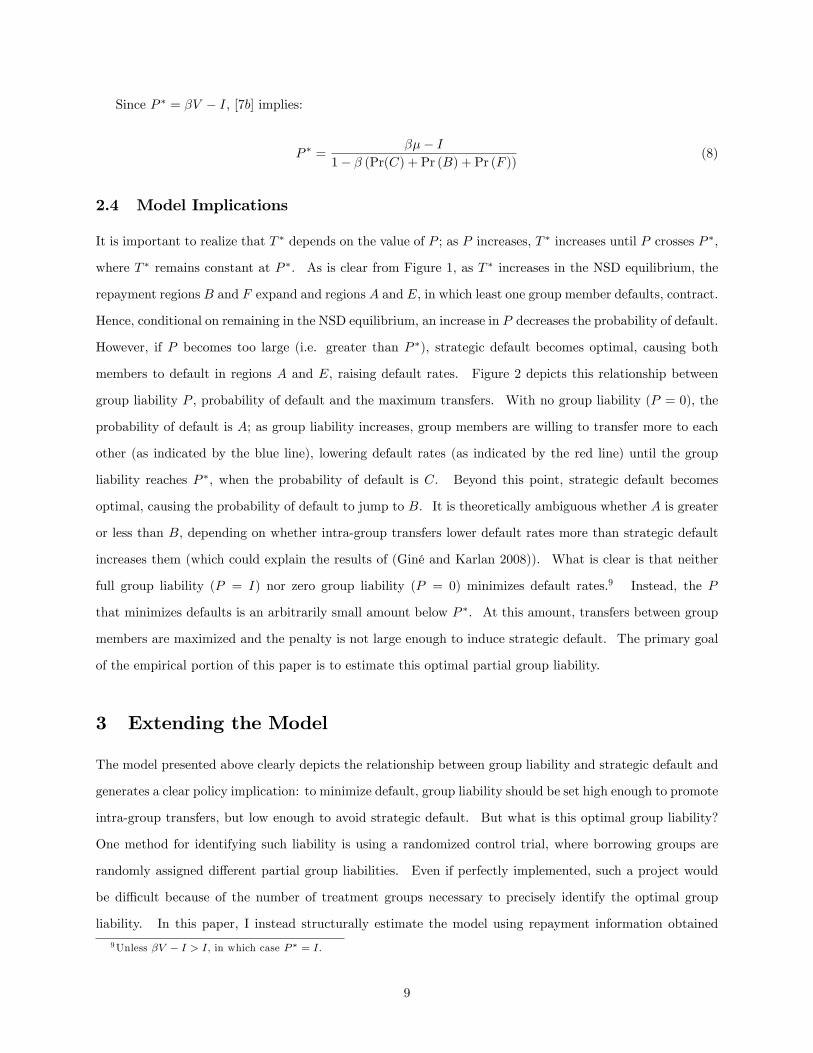
Given the optimal maximum transfers, it is possible to determine whether or not i and g(i) repay

based entirely on the realized returns Ri, Rg(i), the maximum transfers between group members, and the

equilibrium. This is depicted graphically in Figure 1. In region B, g(i) will be transferring funds to i;

similarly, in region F , i will be transferring funds to g(i). In either case, both will repay. In region C,

both i and g(i) will repay without the need of transfers. If the returns are in region D, neither i nor g(i)

will repay. In regions A and E, g(i) or i, respectively, will repay if and only if the group is in the NSD

equilibrium.

2.3 Stage 1: Choosing Whether or Not to Borrow

In the �rst stage, eligible individuals choose whether or not borrow prior to their returns being realized.

With the outside option normalized to 0, individuals will choose to borrow as long as V > 0. Given the

discussion above and the assumption that �� > I, it is straightforward to show V > 0, where for simplicity

of notation, the areas in Figure 1 are made reference to. Note that the optimal transfers are implicitly given

by these areas:

V =E (Ri) + (Pr(C) + Pr (B) + Pr (F )) (�V � I)� � Pr (B)

�I � E

�Rg(i)jB

��+� Pr (F ) (I � E (RijF )) + � Pr (A)max (0; �V � I � P )

(5a)

= �+ (Pr(C) + Pr (B) + Pr (F )) (�V � I) + � Pr (A)max (0; �V � I � P ) (5b)

� �+ (Pr(C) + Pr (B) + Pr (F )) (�V � I) (5c)

=�� (Pr(C) + Pr (B) + Pr (F )) I1� � (Pr(C) + Pr (B) + Pr (F )) > 0 (5d)

7An astute reader might wonder if a cooperative equilibrium where borrowers are willing to transfer more than T � may besustained, similar to the risk sharing models of (Coate and Ravallion 1993) or (Ligon, Thomas, and Worrall 2002). It turns outthat such agreements are not possible because the value of the increase in the probability of future repayment is substantiallysmaller than the cost to the borrower called upon to make a painful transfer. In particular, it can be shown that if the distributionof returns is such that moderate returns are more likely than extreme returns and 1

4>

�(1��)(1��A)T

�f (I + T �; I � T �), where Ais the probability that both borrowers are able to repay; then no cooperative equilibrium where maximum transfers are greaterthan T � can occur. T �f (I + T �; I � T �) will be very small under reasonable parameter assumptions.

7

I

I

I+T*

I+T*Ri

Rg(i)

I­T*

I­T*

A

B C

DE

F

Figure 1: Returns to Borrowing and Defaults in the Basic Model

where the second line used the fact that transfers are symmetric and hence expected transfers are zero

and the last line uses �� > I.8 Note too that:

V � �+ (Pr(C) + Pr (B) + Pr (F )) (�V � I) =) (6a)

�V � I � ��+ � (Pr(C) + Pr (B) + Pr (F )) (�V � I)� I =) (6b)

�V � I � ��� I1� � (Pr(C) + Pr (B) + Pr (F )) > 0 (6c)

This proves the claim above that if �� > I, then �V � I > 0.

If P = P �, then from [5b], we have:

V = �+ (Pr(C) + Pr (B) + Pr (F )) (�V � I), (7a)

V =�� (Pr(C) + Pr (B) + Pr (F )) I1� � (Pr(C) + Pr (B) + Pr (F )) (7b)

8The equation is implicit since the areas of default and repayment depend on T �, which depends on V in the strategic defaultequilibrium.

8

Since P � = �V � I; [7b] implies:

P � =��� I

1� � (Pr(C) + Pr (B) + Pr (F )) (8)

2.4 Model Implications

It is important to realize that T � depends on the value of P ; as P increases, T � increases until P crosses P �,

where T � remains constant at P �. As is clear from Figure 1, as T � increases in the NSD equilibrium, the

repayment regions B and F expand and regions A and E, in which least one group member defaults, contract.

Hence, conditional on remaining in the NSD equilibrium, an increase in P decreases the probability of default.

However, if P becomes too large (i.e. greater than P �), strategic default becomes optimal, causing both

members to default in regions A and E, raising default rates. Figure 2 depicts this relationship between

group liability P , probability of default and the maximum transfers. With no group liability (P = 0), the

probability of default is A; as group liability increases, group members are willing to transfer more to each

other (as indicated by the blue line), lowering default rates (as indicated by the red line) until the group

liability reaches P �, when the probability of default is C. Beyond this point, strategic default becomes

optimal, causing the probability of default to jump to B. It is theoretically ambiguous whether A is greater

or less than B, depending on whether intra-group transfers lower default rates more than strategic default

increases them (which could explain the results of (Giné and Karlan 2008)). What is clear is that neither

full group liability (P = I) nor zero group liability (P = 0) minimizes default rates.9 Instead, the P

that minimizes defaults is an arbitrarily small amount below P �. At this amount, transfers between group

members are maximized and the penalty is not large enough to induce strategic default. The primary goal

of the empirical portion of this paper is to estimate this optimal partial group liability.

3 Extending the Model

The model presented above clearly depicts the relationship between group liability and strategic default and

generates a clear policy implication: to minimize default, group liability should be set high enough to promote

intra-group transfers, but low enough to avoid strategic default. But what is this optimal group liability?

One method for identifying such liability is using a randomized control trial, where borrowing groups are

randomly assigned di¤erent partial group liabilities. Even if perfectly implemented, such a project would

be di¢ cult because of the number of treatment groups necessary to precisely identify the optimal group

liability. In this paper, I instead structurally estimate the model using repayment information obtained

9Unless �V � I > I, in which case P � = I.

9

Figure 2: The E¤ect of Group Liability on the Probability of Default and Transfers

from a large micro�nance institution. Such a methodology generates precise estimates with minimal data

requirements: all that is needs to be observed is who repays and who defaults in a group loan. Hence,

the procedure developed in the remainder of the paper can (and should!) be replicated in other empirical

contexts to assess the robustness of the �ndings.

Unfortunately, the basic model is under-identi�ed and structural estimation is impossible using only data

on whether each group member repays or defaults. This is because of the inability to disentangle correlated

stochastic returns to borrowing between group members and strategic default. Intuitively, just because

it is observed in the data that any time one group member defaults, all other group members default, it

cannot be claimed that strategic default is present - it could very well be that group members have highly

correlated shocks, so when one gets poor returns, all other group members do too. Formally, even after

assuming a particular distribution of returns, the model has (at least) four parameters: � (average returns),

�2 (variance to returns), � (correlation between group members returns) and P (group liability). For each

group, however, only four possible default combinations can be observed: i either defaults or repays and g(i)

either defaults or repays. Given that one event occurs with probability 1, there are three degrees of freedom

to estimate four parameters; the model is under-identi�ed. To overcome this problem, this section of the

paper extends the basic model in two ways: �rst, household structure is incorporated into the model and

second, the model is extended to allow for borrowing groups of more than two members.

10

3.1 Household Structure

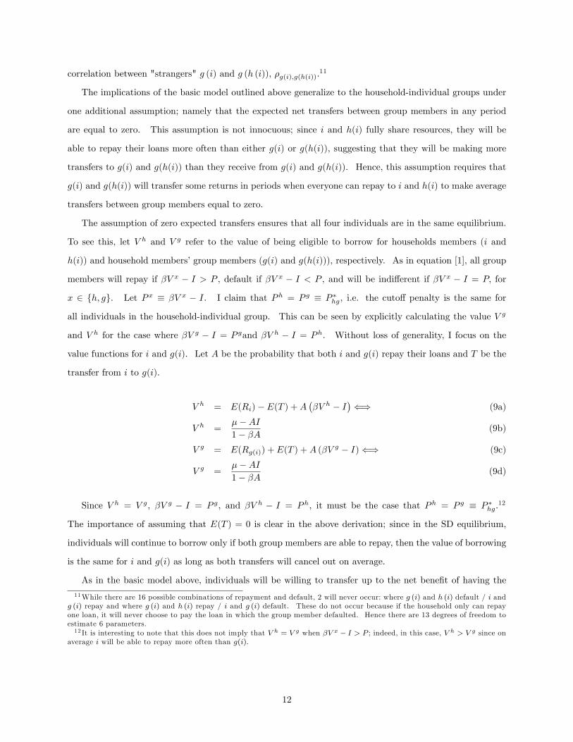
Consider a household with two members, each of whom is in a lending group with an individual in a single-

member household. Let individuals i and h(i) be the two individuals in the two-member household (hereafter

"household members") and let g(i) and g(h(i)) refer to their respective borrowing group members. This

household-group structure, hereafter referred to as "household-individual groups," is illustrated in Figure 3.

i h(i)

g(h(i))g(i) Household­Individual Groups

Figure 3: Household-Individual Group Structure

I assume i and h(i) maximize household returns to borrowing.10 This assumption implies that the

household will pool the returns both receive from borrowing and determine how to best allocate those

returns to the repayment of the two household loans. Given this assumption, extending the basic model

to household-individual groups enables the disentanglement of correlated returns and strategic default by

providing information about how a borrower�s fellow household member (i.e. h (i)) responds to actions by

a borrower�s group member (i.e. g (i)). Intuitively, if there is strategic default but no correlated returns to

borrowing, when g (i) defaults because Rg(i) is low, h (i) will be more likely to repay, since i will strategically

default and Ri can be used to pay back h (i)�s loan. Conversely, if there is no strategic default but there are

correlated returns, when g (i) defaults (suggesting that Rg(i) is low), h (i) is less likely to repay because Rh(i)

will likely be low too. Formally, focusing on household-individual groups provides 16 possible combinations

of repayments/defaults, while the model can be parameterized (given assumptions on the distribution of

returns) by as few as 6 parameters: the mean � and variance �2 to returns, the group liability penalty P ,

the correlation between group members �i;g(i), the correlation between household members, �i;h(i), and the

10This assumption is implied by household Pareto e¢ ciency. Note that i and h(i) may receive di¤erent proportions of thetotal returns to borrowing under this assumption.

11

correlation between "strangers" g (i) and g (h (i)), �g(i);g(h(i)).11

The implications of the basic model outlined above generalize to the household-individual groups under

one additional assumption; namely that the expected net transfers between group members in any period

are equal to zero. This assumption is not innocuous; since i and h(i) fully share resources, they will be

able to repay their loans more often than either g(i) or g(h(i)), suggesting that they will be making more

transfers to g(i) and g(h(i)) than they receive from g(i) and g(h(i)). Hence, this assumption requires that

g(i) and g(h(i)) will transfer some returns in periods when everyone can repay to i and h(i) to make average

transfers between group members equal to zero.

The assumption of zero expected transfers ensures that all four individuals are in the same equilibrium.

To see this, let V h and V g refer to the value of being eligible to borrow for households members (i and

h(i)) and household members�group members (g(i) and g(h(i))), respectively. As in equation [1], all group

members will repay if �V x � I > P , default if �V x � I < P , and will be indi¤erent if �V x � I = P; for

x 2 fh; gg. Let P x � �V x � I. I claim that Ph = P g � P �hg, i.e. the cuto¤ penalty is the same for

all individuals in the household-individual group. This can be seen by explicitly calculating the value V g

and V h for the case where �V g � I = P gand �V h � I = Ph. Without loss of generality, I focus on the

value functions for i and g(i). Let A be the probability that both i and g(i) repay their loans and T be the

transfer from i to g(i).

V h = E(Ri)� E(T ) +A��V h � I

�() (9a)

V h =��AI1� �A (9b)

V g = E(Rg(i)) + E(T ) +A (�Vg � I)() (9c)

V g =��AI1� �A (9d)

Since V h = V g, �V g � I = P g, and �V h � I = Ph, it must be the case that Ph = P g � P �hg.12

The importance of assuming that E(T ) = 0 is clear in the above derivation; since in the SD equilibrium,

individuals will continue to borrow only if both group members are able to repay, then the value of borrowing

is the same for i and g(i) as long as both transfers will cancel out on average.

As in the basic model above, individuals will be willing to transfer up to the net bene�t of having the

11While there are 16 possible combinations of repayment and default, 2 will never occur: where g (i) and h (i) default / i andg (i) repay and where g (i) and h (i) repay / i and g (i) default. These do not occur because if the household only can repayone loan, it will never choose to pay the loan in which the group member defaulted. Hence there are 13 degrees of freedom toestimate 6 parameters.12 It is interesting to note that this does not imply that V h = V g when �V x � I > P ; indeed, in this case, V h > V g since on

average i will be able to repay more often than g(i).

12

other group member repay. Letting T �hg refer to this maximum transfer, the analogs to [8] and [4] are:

P �hg =��� I1� �A (10)

T �hg = min(P; P �hg) = min

�P;��� I1� �A

�(11)

As in the basic model, the probability of both group members repaying (A) depends on the maximum

transfer between group members, so equation [11] implicitly de�nes T �hg.

Hence, given household returns Rh � Ri + Rh(i), household group member�s returns Rg(i) and Rg(h(i)),

maximum transfers T �, and the equilibrium, it is possible to determine which individuals repay and which

individuals default, just like in the basic model. In particular, Figure 1 can be replicated. Of course, now that

there are three returns to keep track of, the �gure must represent the three dimensional Rh�Rg(i)�Rg(h(i))

space. I dissect this three dimensional space into cross sections along the Rh axis in �gures, available in an

online appendix.13 The appendix maps 44 areas in the three dimensional space to default outcomes for all

four individuals in each equilibrium.14

3.2 Groups with more than 2 members

Empirically, most borrowing groups are substantially larger than two members; hence, the basic model and

its household structure extension simplify substantially. Unfortunately, modeling borrowing groups larger

than two complicates the analysis considerably, as the number of possible combinations of default (strategic

or otherwise) increase exponentially. As a compromise between complication and verisimilitude, this section

extends the basic model to include multiple group members by assuming that each individual in the group

treats the other group members like a single group member who has taken out multiple loans. The advantage

of such an extension is that the basic strategies and intuition remain unchanged while allowing the empirical

estimation strategy below to incorporate the size of the borrowing group. The disadvantage is that such a

method e¤ectively assumes that all other group members share a common budget. While this seems like an

egregious simpli�cation, I will argue below that such an assumption will actually lead to estimates that bias

the extent of strategic default downwards, working against my central claim of the importance of addressing

strategic default. In what follows, I refer to this model as the "multiple group member" model.

Extending the basic model to incorporate more than 2 group members enables the disentanglement of

correlated returns from strategic default by allowing the observation of combinations of defaults within a

13Available at http://pantheon.yale.edu/~dwa6/Working%20Papers/Working.htm14 In the case where the household is only able to repay one of the two loans and both g (i) and g (h (i)) are able to repay, it

is assumed that the household chooses one of the loans to repay with probability 12. This is optimal since the household is

indi¤erent about which loan to repay.

13

group. Intuitively, if groups equitably share the liability when a member defaults, then the larger the group,

the smaller the penalty that will be incurred by each individual member when a single member defaults, but

the greater the penalty that will be incurred by an individual when all other group members default. Hence,

in the presence of strategic default, one should expect that in large groups, there will exist some threshold

of number of group members that an individual will tolerate defaulting, above which all group members will

default. Conversely, if there is no strategic default but returns to borrowing are highly correlated, no such

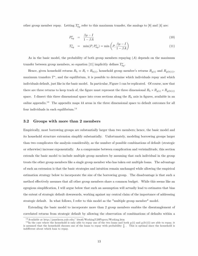
threshold would exist. Table 1 depicts the percentage of group members that default by group size when a

single group member defaults. The table appears to be more consistent with a story of strategic default than

correlated returns to borrowing. While in the vast majority of cases, when one group member defaulted, the

entire group defaulted, one or two group members defaulting occurred more frequently than all but one or

two group members defaulting, and this e¤ect becomes more pronounced as the size of the borrowing group

increases (although the number of observations decline). This, of course, is merely descriptive evidence that

motivates the structural estimation of the model.

Table 1: Observed Composition of Defaults by Group SizeNumber of Members in Borrowing Group

Defaultingmembers 2 3 4 5 6 7 8

1 14.08% 13.93% 7.81% 6.90% 0% 14.29% 0%2 85.92% 7.38% 6.25% 6.90% 5.26% 0% 0%3 78.69% 3.13% 0% 0% 0% 0%4 82.81% 0% 0% 0% 0%5 86.21% 0% 0% 0%6 94.74% 0% 0%7 85.71% 0%8 100.00%

Each column is a di¤erent group size. Each row indicates the number of groupmembers that defaulted (conditional on there being one default). Full sample.

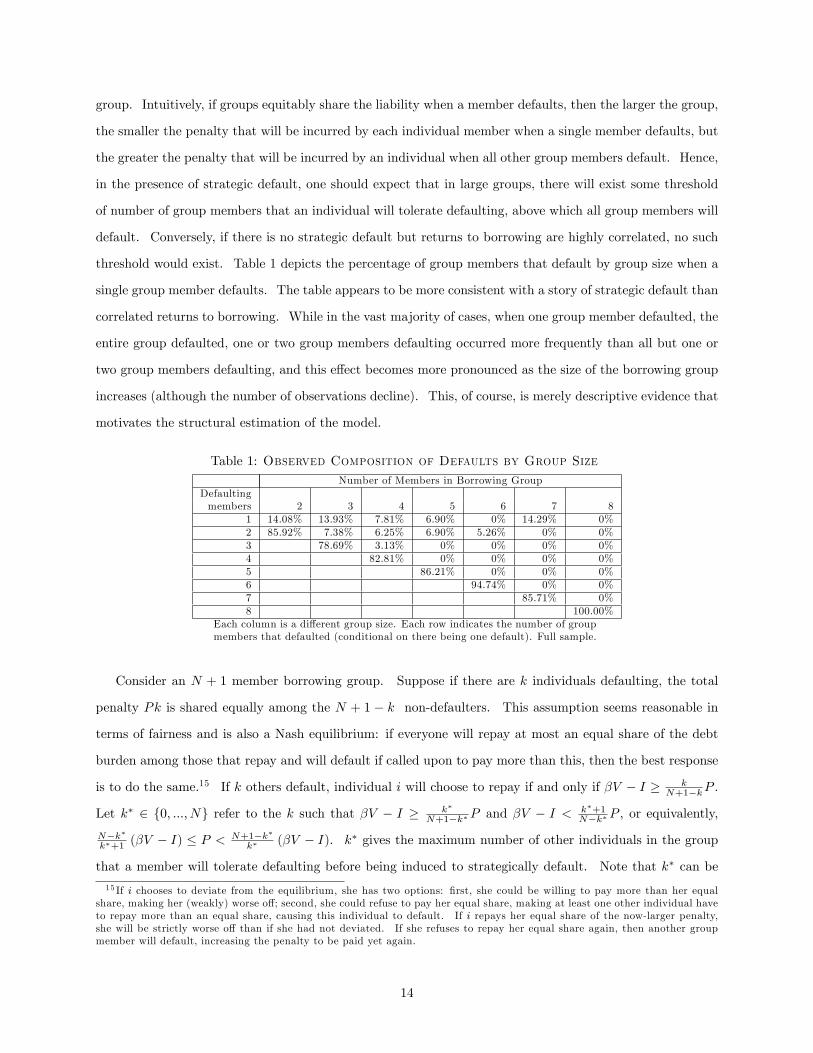
Consider an N + 1 member borrowing group. Suppose if there are k individuals defaulting, the total

penalty Pk is shared equally among the N + 1 � k non-defaulters. This assumption seems reasonable in

terms of fairness and is also a Nash equilibrium: if everyone will repay at most an equal share of the debt

burden among those that repay and will default if called upon to pay more than this, then the best response

is to do the same.15 If k others default, individual i will choose to repay if and only if �V � I � kN+1�kP .

Let k� 2 f0; :::; Ng refer to the k such that �V � I � k�

N+1�k�P and �V � I < k�+1N�k�P , or equivalently,

N�k�k�+1 (�V � I) � P <

N+1�k�k� (�V � I). k� gives the maximum number of other individuals in the group

that a member will tolerate defaulting before being induced to strategically default. Note that k� can be

15 If i chooses to deviate from the equilibrium, she has two options: �rst, she could be willing to pay more than her equalshare, making her (weakly) worse o¤; second, she could refuse to pay her equal share, making at least one other individual haveto repay more than an equal share, causing this individual to default. If i repays her equal share of the now-larger penalty,she will be strictly worse o¤ than if she had not deviated. If she refuses to repay her equal share again, then another groupmember will default, increasing the penalty to be paid yet again.

14

solved in terms of P :N � P

(�V�I)P

(�V�I) + 1� k� < N + 1

1 + P(�V�I)

(12)

From individual i�s perspective, let the sum of the N other group members returns be Rg(i). Suppose

that if aI � Rg(i) < (a+ 1) I, then the rest of the group can at most repay a of its loans without transfers.

This assumption makes the problem computationally feasible by mapping the RN space of returns of the

N di¤erent group members to R space, but comes at the cost of assuming that the distribution of returns

between the other group members does not matter; equivalently, from each individual group member�s

perspective, the rest of the group is sharing their returns and repaying (at most) the maximum number of

loans that the sum of their returns allows them to a¤ord. Such an assumption will of course underestimate

the number of loans that will be defaulted. Since the greater the number of loans that group members

have defaulted on, the greater the incentive to strategically default, this assumption biases downward the

estimates of strategic default. Hence the empirical results following from this estimation technique can be

considered a lower bound on the incidence of strategic default.

To determine transfers, consider the case where aI � Rg(i) < (a+ 1) I and Ri � I +�(a+ 1) I �Rg(i)

�;

i.e. i is determining whether or not to send a transfer to the rest of the group so that they can repay

a + 1 loans instead of a loans. If N � (a+ 1) < k�; i will not transfer anything since even if a + 1 other

group members could repay, they would choose not to since they are in the strategic default equilibrium. If

N � (a+ 1) = k�; then i has an important decision to make: if she transfers enough money so that a+1 will

repay, then there will be k� total defaulters, and all the other borrowers will choose to repay. If she does

not transfer the money, there will be k� + 1 defaulters and everyone will choose to strategically default. In

the former case, she will receive (excluding her returns which she keeps regardless) �V � I � T � k�

N+1�k�P ;

in the latter case, she receives nothing. Hence she will, at most, be willing to transfer �V � I � k�

N+1�k�P .

If N � (a+ 1) > k�, then i; by making a transfer, will be merely avoiding having to pay some share of the

of a penalty. If N � a others default, she would have to pay N�aa+1 P , whereas if she covers a group member

so that only N � (a+ 1) others default, she would have to pay N�(a+1)a+2 P . Hence, she would be willing to

transfer at most�N�aa+1 �

N�(a+1)a+2

�P: Note that if a = N � 1 (that is, all but one other group members can

repay), this simpli�es to PN ; i.e. i would be willing to transfer up to

PN to help the last person pay, since if

that person defaulted, i would be penalized PN .

Figures 7, 9, and 8 included in the appendix depict graphically the di¤erent combinations of default and

repayment given the realized returns Ri and Rg(i). Note that the regions in which "some g (i) default"

are actually combinations of many smaller regions giving the exact number of loans on which g (i) defaults;

the structural estimation of the model uses these exact regions rather than the more easily interpretable

15

aggregate regions pictured.

In Figure 7, the group liability penalty P is su¢ ciently small such that individual i would be willing to

repay even if all other group members defaulted; hence, there is no strategic default. Figure 8 depicts the

opposite extreme, where the group liability penalty P is su¢ ciently large such that individual i would be

unwilling to tolerate even one group member defaulting; hence, either the whole group repays or the whole

group defaults. Figure 9 presents the intermediate case, where P is a moderate size such that individual i

would be willing to tolerate up to k� other group members defaulting; if any more than k� default, i will

choose to strategically default.

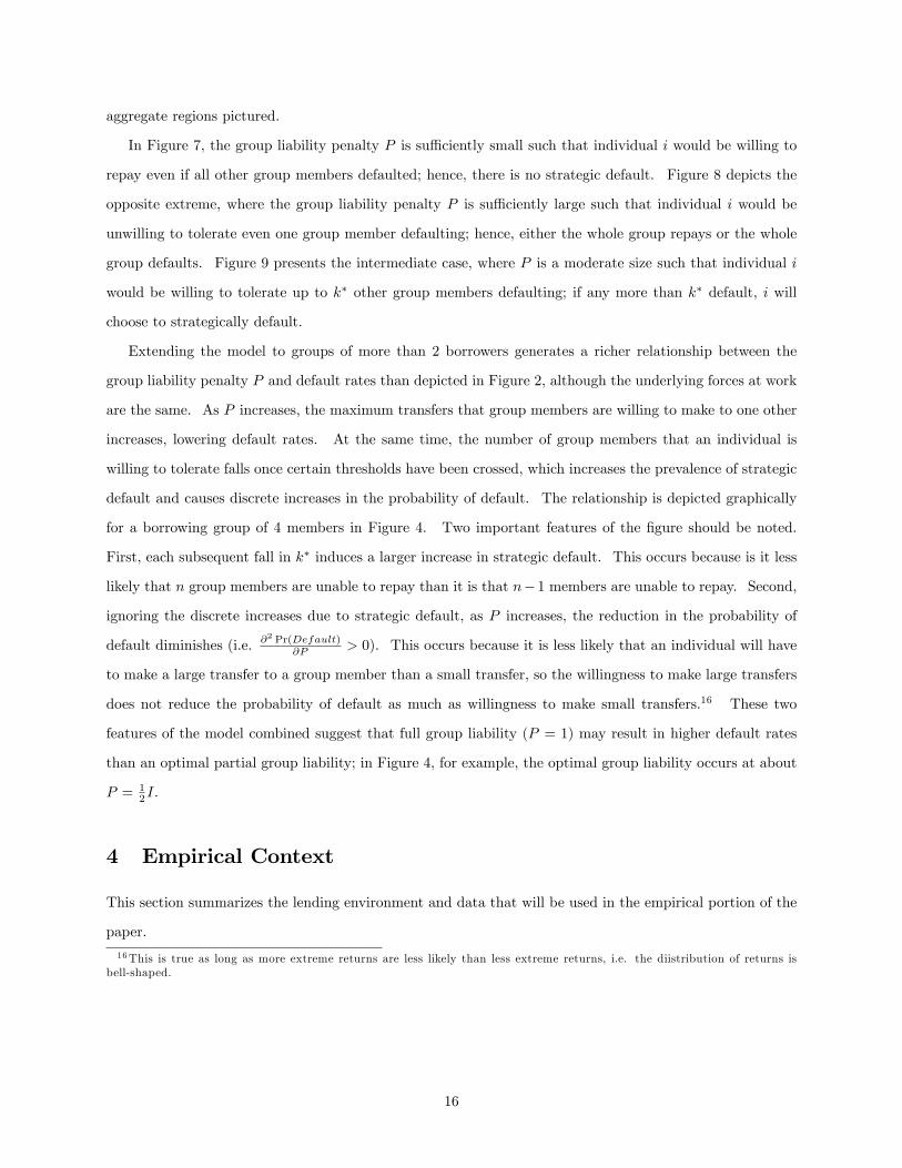
Extending the model to groups of more than 2 borrowers generates a richer relationship between the

group liability penalty P and default rates than depicted in Figure 2, although the underlying forces at work

are the same. As P increases, the maximum transfers that group members are willing to make to one other

increases, lowering default rates. At the same time, the number of group members that an individual is

willing to tolerate falls once certain thresholds have been crossed, which increases the prevalence of strategic

default and causes discrete increases in the probability of default. The relationship is depicted graphically

for a borrowing group of 4 members in Figure 4. Two important features of the �gure should be noted.

First, each subsequent fall in k� induces a larger increase in strategic default. This occurs because is it less

likely that n group members are unable to repay than it is that n�1 members are unable to repay. Second,

ignoring the discrete increases due to strategic default, as P increases, the reduction in the probability of

default diminishes (i.e. @2 Pr(Default)

@P > 0). This occurs because it is less likely that an individual will have

to make a large transfer to a group member than a small transfer, so the willingness to make large transfers

does not reduce the probability of default as much as willingness to make small transfers.16 These two

features of the model combined suggest that full group liability (P = 1) may result in higher default rates

than an optimal partial group liability; in Figure 4, for example, the optimal group liability occurs at about

P = 12I.

4 Empirical Context

This section summarizes the lending environment and data that will be used in the empirical portion of the

paper.

16This is true as long as more extreme returns are less likely than less extreme returns, i.e. the diistribution of returns isbell-shaped.

16

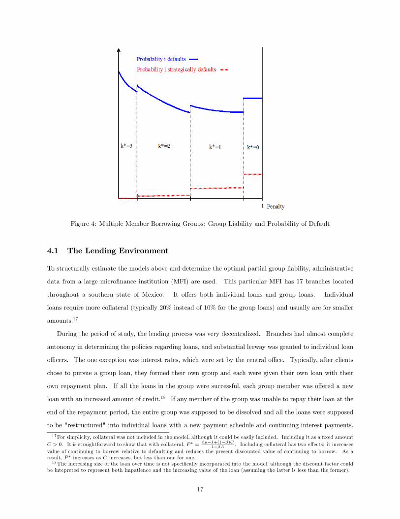
Figure 4: Multiple Member Borrowing Groups: Group Liability and Probability of Default

4.1 The Lending Environment

To structurally estimate the models above and determine the optimal partial group liability, administrative

data from a large micro�nance institution (MFI) are used. This particular MFI has 17 branches located

throughout a southern state of Mexico. It o¤ers both individual loans and group loans. Individual

loans require more collateral (typically 20% instead of 10% for the group loans) and usually are for smaller

amounts.17

During the period of study, the lending process was very decentralized. Branches had almost complete

autonomy in determining the policies regarding loans, and substantial leeway was granted to individual loan

o¢ cers. The one exception was interest rates, which were set by the central o¢ ce. Typically, after clients

chose to pursue a group loan, they formed their own group and each were given their own loan with their

own repayment plan. If all the loans in the group were successful, each group member was o¤ered a new

loan with an increased amount of credit.18 If any member of the group was unable to repay their loan at the

end of the repayment period, the entire group was supposed to be dissolved and all the loans were supposed

to be "restructured" into individual loans with a new payment schedule and continuing interest payments.

17For simplicity, collateral was not included in the model, although it could be easily included. Including it as a �xed amountC > 0. It is straightforward to show that with collateral, P � = ���I+(1��)C

1��A . Including collateral has two e¤ects: it increasesvalue of continuing to borrow relative to defaulting and reduces the present discounted value of continuing to borrow. As aresult, P � increases as C increases, but less than one for one.18The increasing size of the loan over time is not speci�cally incorporated into the model, although the discount factor could

be intepreted to represent both impatience and the increasing value of the loan (assuming the latter is less than the former).

17

Once restructured, an individual must have repaid the restructured loan to be able to continue to borrow.

However, as emphasized by qualitative interviews with the General Director and several branch managers,

there was a substantial amount of �exibility regarding the default process. In some cases, if one group

member failed to repay, the group was allowed to continue without that group member. In other cases,

individuals who had been restructured were discouraged from continuing to borrow, even after repaying.

There were also cases where borrowers were not allowed to continue to borrow until all group members had

repaid their restructured loans in full. The speci�c penalty to having a group member fail to repay was

determined by the loan o¢ cer. Hence, qualitative evidence suggests that the value of P varied substantially

and was ultimately set by the loan o¢ cer. This variation in P across loan o¢ cers is central to the empirical

analysis.

4.2 Data

The administrative data include every loan made by the MFI between 2004 and 2008. During this period,

over 33,000 loans were made to over 18,000 individuals in over 5,000 groups. The data include the start

and end dates of the loan, the amount of the loan (principle and interest), some basic information about

the client, the borrowing group, and whether or not the loan was repaid. Summary statistics for the entire

sample are presented in Table 4 in the appendix. The average loan amount was slightly more than 10,000

pesos (1 US dollar is worth approximately 10 pesos). The default rate was relatively low (4.5%), which is

similar to default rates in other micro�nance lending programs worldwide (Morduch 1999).

The following structural estimation uses only a subset of the administrative data representing loans taken

out by household members in household-individual groups. Speci�cally, the sample includes only loans by

borrowers in which another member of the household had a loan with a di¤erent group at the same time.

Households are de�ned to comprise of all borrowers that have the same address in the same town; addresses

with more than 6 borrowers are excluded as they are unlikely to be considered households in the traditional

sense. Of the 33,772 total loans, 1,782 are included in this sample. Table 5 in the appendix depicts the

summary statistics for this reduced sample; the values of the variables are quite similar to those of the entire

database, although default rates and loan amounts are slightly lower, and the number of group members is

slightly higher. Note that there is no need to constrain my focus to this particular sample for the multiple

group member model; I choose to do so both to retain comparability with the household-individual model

results and to exploit the possibility of out-of-sample tests.

There are at least two potential issues using this sample frame to estimate the household-individual

group modeled above. First, in the model, all four individuals make the decisions of whether or not to

18

repay simultaneously; however, in the data, di¤erent household members�loans start and end at di¤erent

times. In creating this sample, I assume that any loans that overlapped (i.e. one began before the other

ended) occur at the same time. Since most loans are six months in length (see Table 5), this could mean

that the decisions on whether or not to repay may be made multiple months apart. The second problem

arises from the fact that the model only considers four individuals, whereas empirically the number of group

members and often the number of household members is larger. In the estimation below, the "other" group

or household members are simply amalgamated into one individual. Note that neither of these problems

plague the estimation of the multiple group member model. Structural estimation of the multiple group

member model does exclude all groups with more than 13 members because of computation time; these

individuals comprise less than 5% of the sample.

5 Structural Estimation of the Models

5.1 Methodology

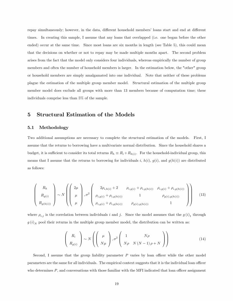
Two additional assumptions are necessary to complete the structural estimation of the models. First, I

assume that the returns to borrowing have a multivariate normal distribution. Since the household shares a

budget, it is su¢ cient to consider its total returns Rh � Ri+Rh(i). For the household-individual group, this

means that I assume that the returns to borrowing for individuals i, h(i), g(i), and g(h(i)) are distributed

as follows:

0BBBB@Rh

Rg(i)

Rg(h(i))

1CCCCA � N

0BBBB@0BBBB@2�

�

�

1CCCCA ; �20BBBB@

2�i;h(i) + 2 �i;g(i) + �i;g(h(i)) �i;g(i) + �i;g(h(i))

�i;g(i) + �i;g(h(i)) 1 �g(i);g(h(i))

�i;g(i) + �i;g(h(i)) �g(i);g(h(i)) 1

1CCCCA1CCCCA (13)

where �i;j is the correlation between individuals i and j. Since the model assumes that the g (i)1 through

g (i)N pool their returns in the multiple group member model, the distribution can be written as:

0B@ Ri

Rg(i)

1CA � N

0B@0B@ �

N�

1CA ; �20B@ 1 N�

N� N (N � 1) �+N

1CA1CA (14)

Second, I assume that the group liability parameter P varies by loan o¢ cer while the other model

parameters are the same for all individuals. The empirical context suggests that it is the individual loan o¢ cer

who determines P , and conversations with those familiar with the MFI indicated that loan o¢ cer assignment

19

was plausibly random within a given branch, providing credence to this assumption. However, since loan

o¢ cers worked only at one branch and the characteristics of borrowers were likely di¤erent depending on

the branch, this assumption is realistic only comparing borrowers within a given branch. Ideally, I would

estimate the model separately for each branch. Unfortunately, there are insu¢ cient observations to do so.

I address this problem below by including branch �xed e¤ects in one speci�cation of the out of sample tests.

These assumptions narrow the set of model parameters to estimate to �; I; �; �2; �; and Po for the multiple

group member model and �; I; �; �2; �i;g(i); �i;h(i) and �g(i);g(h(i)) for the household-individual model, where

Po is the group liability parameter for loan o¢ cer o. I set the discount parameter � = :9 and normalize

I = 1, so that � � 1 gives the expected returns to borrowing as a percentage of the loan and P gives the

group liability as a percentage of the group member�s loan. This leaves 3 + L (5 + L in the household-

individual model) parameters to be estimated, where L is the number of loan o¢ cers (L = 58). Let

�mg ���; �2; �

�and �hh �

��; �2; �i;g(i); �i;h(i); �g(i);g(h(i))

�; i.e. �mg and �hh contain all the parameters

needing to be estimated other than Po for the multiple group member model and the household-individual

model, respectively. Note that if Po > P �hg, then regardless of its speci�c value, the household-individual

model predictions are identical; hence the speci�c value of Po will be unidenti�ed for loan o¢ cers setting the

group liability high enough to cause strategic default. This is not an issue for the multiple group member

model.

I estimate both models using Maximum Likelihood (ML). Let Di be an dummy variable equal to 1 if i

defaulted. For each loan in the sample, I observe the loan o¢ cer (l), group size (N +1), whether or not the

individual defaulted (Di), how many of the individual�s group members defaulted (PN

j=1Dg(i)j ), whether or

not any of the individual�s household members defaulted (Dh(i)), and whether or not any of the individual�s

household member�s group members defaulted (Dg(h(i))). The multiple group member model only uses the

information about N , Di, andPN

j=1Dg(i)j . The household-individual model only uses information about

Di, whether or not any of the other group members defaulted (1�PN

j=1Dg(i)j � 1�), Dh(i), and Dg(h(i)).19

For a given �mg and P , the probability of observing any one of the possible 2N+1 combinations of

repayments and defaults in the multiple group member model can be calculated. Similarly, for a given

�hh and P , the probability of observing any one of the possible 24 combinations of repayments and defaults

in the household-individual model can be calculated. Let Don refer to the observed default combination

of the nth borrower who with loan o¢ cer o, and let No be the number of borrowers that loan o¢ cer o

oversees. Let lmg(D; �; P ) and lhh (D; �; P ) be the probability of observing a particular default combination

19Considering any group member (or household member or household member�s group member) defaulting as a default isnecessary to map many member households and groups into the simpli�ed 4 individual household-individual group structurepictured in Figure 3. Given that the vast majority of defaults are group wide (see Table 1), this assumption is not as problematicas may �rst appear. Because it is an oversimplication of reality, however, it is important to pursue two distinct methods ofestimation to get insight on how much such simplications a¤ect the results.

20

D given parameters � and penalty P in the multiple group member model and household-individual model,

respectively. Then the total likelihood functions for the multiple group member model and the household-

individual model can be written (in logs) as:

ln [Lmg (�)] =LXo=1

max

maxP2[0;1]

NoXn=1

ln [lmg(Don; �; P )]

!(15a)

ln�Lhh (�)

�=

LXo=1

max

max

P2[0;P�hg(�)]

NoXn=1

ln [l(Don; �; P )] ;

NoXn=1

ln�l(Do

n; �; P > P�hg (�))

�!(15b)

The di¤erence between equations [15a] and [15b] comes from the fact that in the household-individual

model, when P > P �hg, the predicted probabilities are the same regardless of the P . Hence, a point estimate

of such a P can not occur. Since each loan o¢ cer has his or her own penalty, all household-individual

borrowers with the same loan o¢ cer are in the same equilibrium. To estimate which equilibrium each loan

o¢ cer is in, I take the maximum log likelihood over all possible value of Po less than P �hg (which can be

calculated given � using [10]) and compare it to the log likelihood if Po � P �hg. If the latter is greater than

the former, the loan o¢ cer will be estimated to be in the SD equilibrium.20

The ML estimates of � are de�ned as:

�mg

� argmax�2�

ln [Lmg (�)] (16a)

�hh

� argmax�2�

ln�Lhh (�)

�(16b)

The estimated penalty for each loan o¢ cer is de�ned as:

Pmgo � arg maxP2[0;1]

NoXn=1

lnhlmg(Do

n; �mg; P )

i(17a)

Phho ��P �hg ��hh� if maxP2h0;P�

hg

��hh�iPNo

n=1 lnhl(Do

n; �mg; P )

i<PNo

n=1 lnhl(Do

n; �; P > P�hg

��hh�)i

argmaxP2

h0;P�

hg

��hh�iPNo

n=1 lnhlmg(Do

n; �mg; P )

iotherwise

�(17b)

The standard errors for �mg

and �hh, respectively, that are reported below are estimated by taking the

square root of the diagonals of the variance-covariance matrix estimated by the negative of the inverse of

20 In the empirical analysis below, such loan o¢ cers are assigned a P = P �hg , even though their P is not point identi�ed and

could be anywhere between P �hg and 1. Since P �hg = :87, this arbitrary assignment does not likely have a large e¤ect on theestimates.

21

the Hessian of the log likelihood function evaluated at the estimated parameters:

= �

0@@2 lnhL���i

@�@�0

1A�1

(18)

This standard procedure, however, fails to account for the fact that thenPmgo

oLo=1

andnPhho

oLo=1

were

maximized in an inner step in Lmg (�) and Lhh (�) ; respectively.21 While this produces consistent and

unbiased estimates, the standard procedure for calculating standard errors is not correct. The best way of

correcting the standard errors would be to use a nonparametric bootstrapping procedure; however, given that

the structural estimation of each model takes about 12 hours to run on a high speed computing cluster, such

a procedure is computationally infeasible. Hence, the absurdly precise standard errors of model parameters

presented in the results below should be interpreted with caution.

5.2 Structural Estimation Results

Table 2 presents the structural estimates of the underlying model parameters. These results appear realistic

and are estimated very precisely (although recall that the standard errors fail to account for the inner

maximization of loan o¢ cer speci�c penalties). The returns to borrowing, net of interest costs, are 26.7%

per loan in the household-individual model and 44.6% per loan in the multiple group member model. Since

each loan is approximately 6 months long and the annual interest rate is about 46%, this suggests that the

gross monthly returns to borrowing are 7:10% ( ln(1:267)6 + ln(1:46)12 ) and 9:30% ( ln(1:446)6 + ln(1:46)

12 ), which is very

similar to experimental estimates of the returns to borrowing among small business owners in other developing

countries (de Mel, McKenzie, and Woodru¤ 2008). The variance in returns to borrowing implies a standard

deviation in returns equal to 0:318 and 0:620 for the household-individual and multiple group member models,

respectively, which, given the estimated mean returns and the normal distribution, suggests that a household

member will get negative returns (relative to the principal plus interest) on a loan 20:04% (household-

individual model) to 23:59% (multiple group member model) of the time. The estimated correlation of

returns between group members is virtually zero for the household-individual model, but substantial for the

multiple group member model.

Given the household-individual model parameter estimates, P �hg = :8733. This means that only borrowers

who faced close to full group liability would �nd it optimal to strategically default. Of the 58 loan o¢ cers

in the sample, 45 (who oversaw 68% of total borrowers) were estimated to have penalties greater than P �hg.

21Computationally, the two-step ML process was accomplished by performing a grid search over possible values of P for eachloan o¢ cer given � and selecting the P that maximized the log likelihood for the loan o¢ cer. The sum of the log likelihoodsof the maximized values of P for all loan o¢ cers was then maximized over the space of � using the constrained optimizationfunction fmincon in Matlab.

22

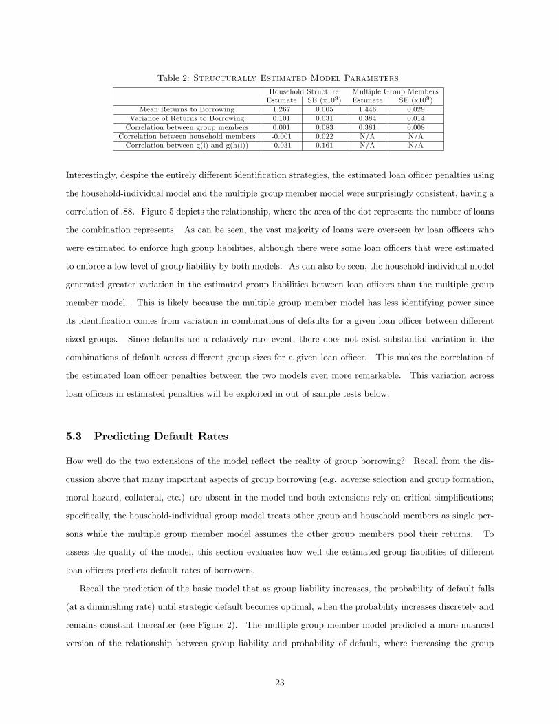
Table 2: Structurally Estimated Model ParametersHousehold Structure Multiple Group MembersEstimate SE (x109) Estimate SE (x109)

Mean Returns to Borrowing 1.267 0.005 1.446 0.029Variance of Returns to Borrowing 0.101 0.031 0.384 0.014Correlation between group members 0.001 0.083 0.381 0.008

Correlation between household members -0.001 0.022 N/A N/ACorrelation between g(i) and g(h(i)) -0.031 0.161 N/A N/A

Interestingly, despite the entirely di¤erent identi�cation strategies, the estimated loan o¢ cer penalties using

the household-individual model and the multiple group member model were surprisingly consistent, having a

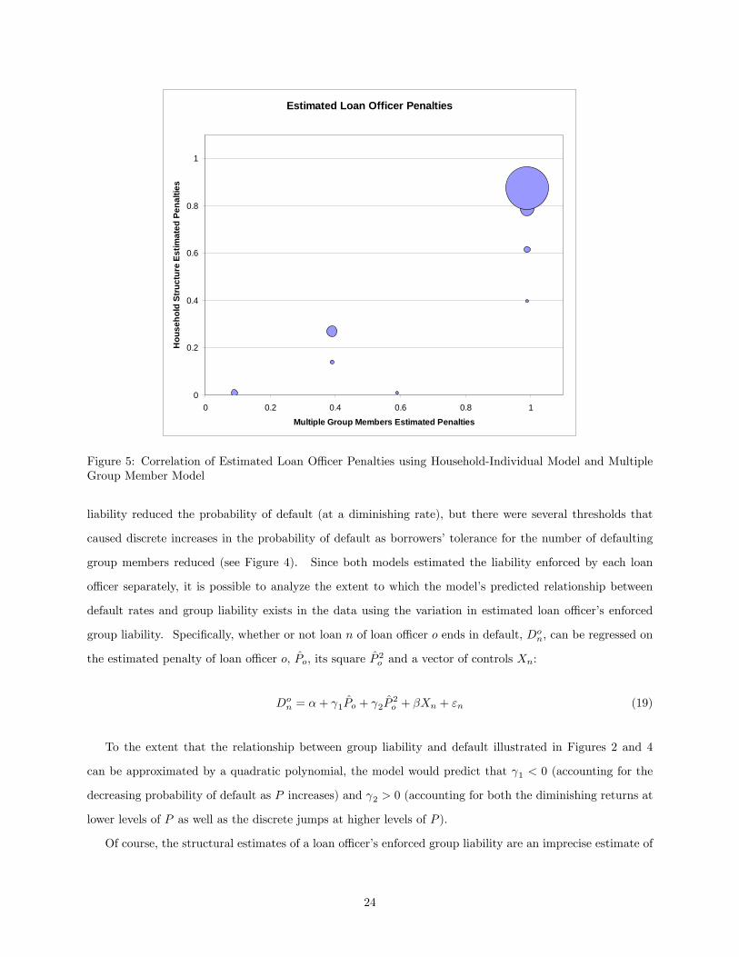
correlation of .88. Figure 5 depicts the relationship, where the area of the dot represents the number of loans

the combination represents. As can be seen, the vast majority of loans were overseen by loan o¢ cers who

were estimated to enforce high group liabilities, although there were some loan o¢ cers that were estimated

to enforce a low level of group liability by both models. As can also be seen, the household-individual model

generated greater variation in the estimated group liabilities between loan o¢ cers than the multiple group

member model. This is likely because the multiple group member model has less identifying power since

its identi�cation comes from variation in combinations of defaults for a given loan o¢ cer between di¤erent

sized groups. Since defaults are a relatively rare event, there does not exist substantial variation in the

combinations of default across di¤erent group sizes for a given loan o¢ cer. This makes the correlation of

the estimated loan o¢ cer penalties between the two models even more remarkable. This variation across

loan o¢ cers in estimated penalties will be exploited in out of sample tests below.

5.3 Predicting Default Rates

How well do the two extensions of the model re�ect the reality of group borrowing? Recall from the dis-

cussion above that many important aspects of group borrowing (e.g. adverse selection and group formation,

moral hazard, collateral, etc.) are absent in the model and both extensions rely on critical simpli�cations;

speci�cally, the household-individual group model treats other group and household members as single per-

sons while the multiple group member model assumes the other group members pool their returns. To

assess the quality of the model, this section evaluates how well the estimated group liabilities of di¤erent

loan o¢ cers predicts default rates of borrowers.

Recall the prediction of the basic model that as group liability increases, the probability of default falls

(at a diminishing rate) until strategic default becomes optimal, when the probability increases discretely and

remains constant thereafter (see Figure 2). The multiple group member model predicted a more nuanced

version of the relationship between group liability and probability of default, where increasing the group

23

Estimated Loan Officer Penalties

0

0.2

0.4

0.6

0.8

1

0 0.2 0.4 0.6 0.8 1

Multiple Group Members Estimated Penalties

Hou

seho

ld S

truc

ture

 Est

imat

ed P

enal

ties

Figure 5: Correlation of Estimated Loan O¢ cer Penalties using Household-Individual Model and MultipleGroup Member Model

liability reduced the probability of default (at a diminishing rate), but there were several thresholds that

caused discrete increases in the probability of default as borrowers�tolerance for the number of defaulting

group members reduced (see Figure 4). Since both models estimated the liability enforced by each loan

o¢ cer separately, it is possible to analyze the extent to which the model�s predicted relationship between

default rates and group liability exists in the data using the variation in estimated loan o¢ cer�s enforced

group liability. Speci�cally, whether or not loan n of loan o¢ cer o ends in default, Don, can be regressed on

the estimated penalty of loan o¢ cer o, Po, its square P 2o and a vector of controls Xn:

Don = �+ 1Po + 2P

2o + �Xn + "n (19)

To the extent that the relationship between group liability and default illustrated in Figures 2 and 4

can be approximated by a quadratic polynomial, the model would predict that 1 < 0 (accounting for the

decreasing probability of default as P increases) and 2 > 0 (accounting for both the diminishing returns at

lower levels of P as well as the discrete jumps at higher levels of P ).

Of course, the structural estimates of a loan o¢ cer�s enforced group liability are an imprecise estimate of

24

the true enforced group liability. If there is substantial measurement error, then estimates of 1 and 2 can

be biased towards zero. Fortunately, there exists two estimates of each loan o¢ cer�s enforced group liability:

one from the household-individual model estimation (Phho ) and one from the multiple group member model

estimation (Pmgo ). Suppose that the true loan o¢ cer o�s enforced group liability is Po and:

Po = Phho + uo (20a)

Po = Pmgo + vo (20b)

uo and vo are and mean zero i.i.d. (20c)

E (uovo) = 0 (20d)

The assumption that E (uovo) = 0 seems reasonable considering that the two models use distinct methods

of identifying a loan o¢ cer�s group liability. If these assumptions hold, then the measurement error bias can

be overcome by instrumenting for one measure of group liability (say Pmgo ) with the other measure (Phho ).22

Of course, observing that 1 < 0 and 2 > 0 using the same loans that were used to structurally estimate

the model is not very convincing evidence of the validity of the model: the estimated parameters and loan

o¢ cer penalties were chosen to make the model match the data! What is needed instead is to see if

1 < 0 and 2 > 0 for loans that the structural estimates were not based upon. Here too I am fortunate;

since the household-individual model could only be estimated for the subset of loans where the borrowers

�t the household/borrowing structure depicted in Figure 3, there exists a large number (25,643) of other

loans overseen by the same loan o¢ cers where the borrowers did not come from households with multiple

household members in di¤erent borrowing groups. For these observations, estimates of the loan o¢ cer�s

enforced group liability exist but the loans themselves were not used to estimate the model. If it is true

that loan o¢ cers have a constant group liability that they apply to all groups and the model�s prediction

regarding the relationship between group liability and defaults is correct, then one would expect to see that

1 < 0 and 2 > 0 for these loans out of sample. (If, however, it is not observed that 1 < 0 and 2 > 0; it

could be either that loan o¢ cers do not enforce a constant group liability or that the model�s prediction is

incorrect.)

For both the household-individual sample ("in sample") and the loans not in the household-individual

sample but sharing the same loan o¢ cers ("out of sample"), I estimate equation [19] using both Phho (columns

labeled "HH") and Pmgo (columns labeled "Group") as well as instrumenting for Pmgo using Phho (columns

labeled "IV"). I consider three di¤erent speci�cations: �rst, I include no control variables; second, I include

22While either measure can legitimately be chosen as the instrument, I have chosen Phho as the instrument because it hasmore variation and hence more predictive power (see �gure 5 and the associated discussion).

25

various individual and loan speci�c control variables as well as time �xed e¤ects; and third, I include all of

these control variables as well as branch �xed e¤ects. The second speci�cation is meant to test to see if

the structural estimates of loan o¢ cer�s enforced group liability merely re�ect di¤erences across loan o¢ cers

in observable characteristics of the loan and borrower. Including branch �xed e¤ects tests to see if the

estimated loan o¢ cer�s penalties merely re�ect di¤erences (observed or unobserved) across branches in loans

and borrowers. Unfortunately, because much of the variation in group liability occurs across branches rather

than within, the power of such a speci�cation is low.

The results of the regressions are presented in Tables 6 and 7 for the "in sample" and "out sample",

respectively. As expected, in the sample used to make the structural estimates, 1 < 0 and 2 > 0

for the household-individual model, and the coe¢ cients are statistically signi�cant for all speci�cations.

Surprisingly, however, the results for the multiple group member model and the instrumented variable

columns are statistically signi�cant in the "wrong" direction, suggesting that default rates increase concavely

as group liability increases. This relationship could re�ect the imprecise estimates of the multiple group

member model (although such an explanation fails to explain why the results are statistically signi�cant as

well as at odds with the model predictions).

In the out of sample loans, the household-individual predicted loan o¢ cer penalties are statistically

signi�cant and consistent with model predictions, even for the restrictive branch �xed e¤ects speci�cation.

Interestingly, despite getting the "wrong" sign in sample, the multiple group member estimated loan o¢ cer

penalties now have the "right" sign out of sample for two of the three speci�cations (although they are

insigni�cant). With branch �xed e¤ects, however, the multiple group member estimated loan o¢ cer penalties

are statistically signi�cant in the "wrong" direction. The IV results are consistent with the model and

statistically signi�cant, except for the branch �xed e¤ects model, which has the "right" sign but is not

statistically signi�cant. The IV results are also larger in magnitude than the other estimates, which is

consistent with the existence of measurement error. That the estimated loan o¢ cer penalties have substantial

predictive ability of defaults out of sample and are consistent with model predictions lends substantial support

to the ability of the model to describe the reality of group borrowing despite its simplicity. The results also

lend credence to the assumption that each loan o¢ cer has a constant group liability that she applies to all

the loans she oversees.

One obvious objection to the above results is that estimates of Pmgo and Phho do not re�ect a loan o¢ cer�s

enforced group liability, but rather the quality of the loan o¢ cer. Hence, the results above merely re�ect the

fact that "better" loan o¢ cers have lower default rates. Such a critique is unfounded because the estimates

of Pmgo and Phho do not arise from average default rates, but rather from the particular combination of

defaults, whether it be within households (in the case of Phho ) or within a given group (in the case of Pmgo ).

26

Group Liability and Default Rates

­0.15

­0.1

­0.05

0

0.05

0.1

0.15

0.2

0.25

0.3

0 0.1 0.2 0.3 0.4 0.5 0.6 0.7 0.8 0.9 1

Group Liability (P)

Prob

abili

ty o

f Def

ault

4 Group Members (structural estimate) 13 Group Members (structural estimate) Observed (Group estimated penalties)Observed (Household estimated penalties) Out of Sample IV Regression Household (structural estimate)Out of Sample HH Regression Out of Sample Group Regression

Figure 6: Group Liability and Default Rates

Put another way, two loan o¢ cers with very similar average default rates (and hence of similar "qualities")

may be estimated to have very di¤erent group liabilities depending on the combination in which the defaults

were realized. This is indeed the case, as clearly evident in Figure 6 below, where the red dots show that Phho

varies substantially for a given rate of default. Of course, it could be that loan o¢ cers that have successfully

determined the optimal liability are also better in other unobservable dimensions. If this story is true, then

1 and 2 estimate the combined e¤ect of optimal liability and these other unobservables on default rates.

5.4 Optimal Group Liability

Given the structural estimates and the empirical analysis above, what is the implied optimal group liability?

Figure 6 illustrates the relationship between group liability and default rates implied by structural estimates

of the household-individual model, the structural estimates of the multiple group members model (for both

4 member groups and 13 member groups), and the implied relationship given the estimated coe¢ cients

from the regressions (without controls) in Table 7. It also depicts the average default rates for each of the

estimated loan o¢ cer penalties for both the household-individual model and the multiple group member

model. Table 3 presents the implied optimal group liability for each method.

As can be seen, the estimated optimal liability varies substantially depending on the method. As

mentioned above, the household-individual model structural estimates imply an optimal group liability of

27

87.33%. Interestingly, the group member model structural estimates imply that full group liability is optimal;

this is because the structural estimates suggest that group members are willing to tolerate a relatively

large number of fellow group members defaulting before they are induced to default as well; since it is

relatively unlikely that such an event will occur, the bene�ts of larger group liability outweighs the costs of

strategic default. Recall, however, that the assumption of pooling of returns among "other" group members

underestimates strategic default and hence biases the optimal partial liability toward 100%. The implied

optimal liability from the regression analyses tends to be lower than the implied optimal liability implied by

the structural estimation; disregarding the statistically insigni�cant results and the multiple group member

branch �xed e¤ects result with the "wrong" signs on the coe¢ cients, the estimates range from 54.2% to

67.6%. This, however, could merely be re�ecting the imperfect �t of a quadratic polynomial to the actual

relationship.

Table 3: Estimated Optimal Group LiabilityMethodology Optimal Liability Reduction in Default:

Optimal Liability 75% LiabilityStructural Estimates

Household-Individual 87.33% 2.96% 2.91%Multiple Group Members 100.00% 0.00% -0.68%Out of Sample RegressionsPenalties estimated using Household-Individual Model

No controls 54.73% 11.51% 9.20%Controls 54.22% 11.51% 9.20%

Branch FE 67.56% 12.42% 9.86%Penalties estimated using Multiple Group Members Model

No controls* 67.56% 0.19% 0.10%Controls* 85.41% 0.20% 0.10%Branch FE 100.00% 0.00% -0.75%

IV regressionsNo controls 65.58% 16.55% 15.31%Controls 65.45% 17.01% 15.71%

Branch FE* 85.00% 0.58% 0.32%Astericks indicate the estimated coe¢ cients were statistically insigni�cant."Reduction in Default" columns report the estimated decline in default rates(in percentage points) from full group liability.

Table 3 also depicts the estimated reduction in default (in percentage points) from moving from full group

liability to the optimal group liability and to 75% group liability. Given the observed default rate of 4.5%,

the estimated reduction in default rates is substantial. Of course, for the out of sample regressions, this is

likely just a by-product of the polynomial estimation technique - this is clearly evident in Figure 6, where

certain ranges of liabilities are estimated to have negative default rates. Still, the household-individual

structural estimate suggests that default rates would fall by more than half if the optimal group liability

was adopted - an enormous e¤ect for a relatively small change in policy. Comparing full group liability to

75% group liability demonstrates that the reduction in default is almost as large as moving to the optimal

liability, while for the methods predicting full liability is optimal, the move to 75% liability would increase

28

default rates only minimally. A policy of 75% group liability is also easily explained to potential borrowers

("they borrow 4, you�re responsible for 3"). Of course, these estimates do not account at all for problems

of moral hazard and adverse selection, which would likely be exacerbated as group liability is reduced. It

seems unlikely, however, that the marginal increase in default rates rising from such problems would eclipse

the gains from reduced strategic default, i.e. the discontinuous increase in defaults arising from strategic

default will likely eclipse any e¤ects that are continuous functions of group liability. Put simply, if I am

held responsible for 75% instead of 100% of my group member�s loan, it seems unreasonable to assume that

borrowers would put substantially less e¤ort into choosing good group members and making sure they use

their loans responsibly.

6 Conclusion

This paper developed a model of group lending that contrasts the costs and bene�ts of group liability. The

model implied that greater group liability encourages greater intra-group transfers, but if group liability is

too large, it induces borrowers to strategically default. While simple, the model incorporated several realistic

characteristics of group lending, including correlated stochastic returns to borrowing, limited liability, and

forward-looking behavior. Since the model could not disentangle strategic default from correlated returns

to borrowing using observations on repayments alone, the model was extended in two directions, �rst to

include household structure and second to incorporate borrowing groups of more than two individuals.

Both model extensions were structurally estimated using repayment data from a large micro�nance

institution in southern Mexico. Despite di¤erences in the methods of identi�cation, structural estimates of

model fundamentals were similar in both extensions, suggesting high but variable returns to borrowing. The

multiple borrowing member model also estimated substantial correlation in group member returns, although

the model based on household structure did not. Exploiting the fact that individual loan o¢ cers were largely

able to choose their own policies regarding default, each loan o¢ cer�s de facto group liability was estimated;

these estimates were remarkably similar for the two models, �nding the majority of loan o¢ cers enforced full

group liability and the remaining loan o¢ cers exhibited substantial variation in their degree of group liability

enforcement. Using this variation, the model�s predictions regarding the relationship between group liability

and default rates were tested on loans that were not used to make the structural estimates. Measurement

error was corrected for by instrumenting for one estimate with the other. The out of sample results strongly

supported the conclusion of the model that partial group liability results in lower default rates than either

full group liability or full individual liability. Estimates of the optimal partial group liability ranged from

55% to 100% of full group liability, although 75% group liability was shown to reduce default rates nearly

29

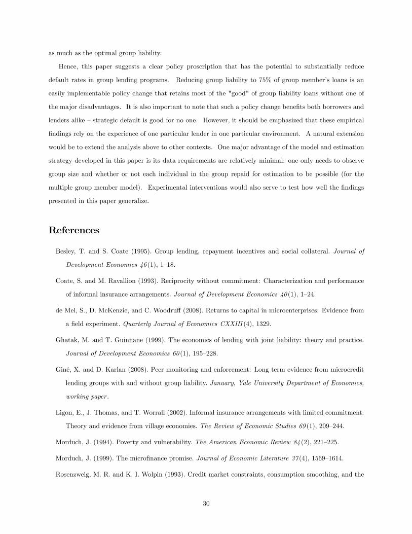
as much as the optimal group liability.

Hence, this paper suggests a clear policy proscription that has the potential to substantially reduce

default rates in group lending programs. Reducing group liability to 75% of group member�s loans is an

easily implementable policy change that retains most of the "good" of group liability loans without one of

the major disadvantages. It is also important to note that such a policy change bene�ts both borrowers and

lenders alike �strategic default is good for no one. However, it should be emphasized that these empirical

�ndings rely on the experience of one particular lender in one particular environment. A natural extension

would be to extend the analysis above to other contexts. One major advantage of the model and estimation

strategy developed in this paper is its data requirements are relatively minimal: one only needs to observe

group size and whether or not each individual in the group repaid for estimation to be possible (for the

multiple group member model). Experimental interventions would also serve to test how well the �ndings

presented in this paper generalize.

References

Besley, T. and S. Coate (1995). Group lending, repayment incentives and social collateral. Journal of

Development Economics 46 (1), 1�18.

Coate, S. and M. Ravallion (1993). Reciprocity without commitment: Characterization and performance

of informal insurance arrangements. Journal of Development Economics 40 (1), 1�24.

de Mel, S., D. McKenzie, and C. Woodru¤ (2008). Returns to capital in microenterprises: Evidence from

a �eld experiment. Quarterly Journal of Economics CXXIII (4), 1329.

Ghatak, M. and T. Guinnane (1999). The economics of lending with joint liability: theory and practice.

Journal of Development Economics 60 (1), 195�228.

Giné, X. and D. Karlan (2008). Peer monitoring and enforcement: Long term evidence from microcredit

lending groups with and without group liability. January, Yale University Department of Economics,

working paper .

Ligon, E., J. Thomas, and T. Worrall (2002). Informal insurance arrangements with limited commitment:

Theory and evidence from village economies. The Review of Economic Studies 69 (1), 209�244.

Morduch, J. (1994). Poverty and vulnerability. The American Economic Review 84 (2), 221�225.

Morduch, J. (1999). The micro�nance promise. Journal of Economic Literature 37 (4), 1569�1614.

Rosenzweig, M. R. and K. I. Wolpin (1993). Credit market constraints, consumption smoothing, and the

30

accumulation of durable production assets in low-income countries: Investments in bullocks in india.

The Journal of Political Economy 101 (2), 223�244.

31

7 Appendix

Table 4: Summary Statistics for all Group LoansVariable Mean (Std. Dev.) Min. Max.

Default 0.045 (0.207) 0 1Age 38.612 (11.44) 13.933 87.441Sex (1=male) 0.181 (0.385) 0 1Loan Amount (pesos) 10036.727 (12145.261) 384.61 260000Tenure with Bank (weeks) 51.208 (33.35) 4.429 311.143Interest Rate (annual) 0.461 (0.052) 0 1.725Loan Length (weeks) 28.417 (6.295) 3.714 107.571Group Size 4.472 (3.437) 2 31

N 33772

Table 5: Summary Statistics for Household Members in Household-Individual GroupsVariable Mean (Std. Dev.) Min. Max.

Default 0.036 (0.186) 0 1Age 38.691 (11.918) 18.209 82.188Sex (1=male) 0.183 (0.387) 0 1Loan Amount (pesos) 9666.183 (8903.115) 763.070 101680Tenure with Bank (weeks) 48.287 (29.625) 13.857 172.286Interest Rate (annual) 0.457 (0.046) 0 0.565Loan Length (weeks) 27.733 (3.836) 13.857 54.143Group Size 5.036 (3.993) 2 27

N 1782

32

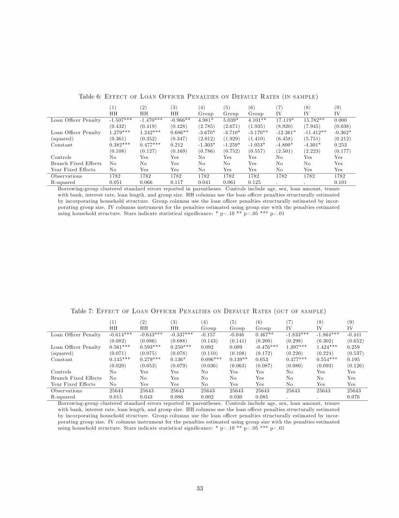
Table 6: Effect of Loan Officer Penalties on Default Rates (in sample)

(1) (2) (3) (4) (5) (6) (7) (8) (9)HH HH HH Group Group Group IV IV IV

Loan O¢ cer Penalty -1.507*** -1.470*** -0.966** 4.981* 5.039* 4.101** 17.119* 15.782** 0.000(0.432) (0.419) (0.428) (2.785) (2.671) (1.935) (8.920) (7.945) (0.038)

Loan O¢ cer Penalty 1.279*** 1.242*** 0.686** -3.670* -3.710* -3.170** -12.361* -11.412** -0.362*(squared) (0.361) (0.352) (0.347) (2.012) (1.929) (1.410) (6.458) (5.751) (0.212)Constant 0.382*** 0.477*** 0.212 -1.303* -1.259* -1.053* -4.800* -4.301* 0.253

(0.108) (0.127) (0.169) (0.786) (0.752) (0.557) (2.501) (2.223) (0.177)Controls No Yes Yes No Yes Yes No Yes YesBranch Fixed E¤ects No No Yes No No Yes No No YesYear Fixed E¤ects No Yes Yes No Yes Yes No Yes YesObservations 1782 1782 1782 1782 1782 1782 1782 1782 1782R-squared 0.051 0.066 0.117 0.041 0.061 0.125 . . 0.101Borrowing-group clustered standard errors reported in parentheses. Controls include age, sex, loan amount, tenurewith bank, interest rate, loan length, and group size. HH columns use the loan o¢ cer penalties structurally estimatedby incorporating household structure. Group columns use the loan o¢ cer penalties structurally estimated by incor-porating group size. IV columns instrument for the penalties estimated using group size with the penalties estimatedusing household structure. Stars indicate statistical signi�cance: * p<.10 ** p<.05 *** p<.01

Table 7: Effect of Loan Officer Penalties on Default Rates (out of sample)

(1) (2) (3) (4) (5) (6) (7) (8) (9)HH HH HH Group Group Group IV IV IV

Loan O¢ cer Penalty -0.614*** -0.643*** -0.337*** -0.157 -0.046 0.467** -1.833*** -1.864*** -0.441(0.082) (0.086) (0.088) (0.143) (0.141) (0.200) (0.298) (0.302) (0.652)

Loan O¢ cer Penalty 0.561*** 0.593*** 0.250*** 0.092 0.009 -0.476*** 1.397*** 1.424*** 0.259(squared) (0.071) (0.075) (0.078) (0.110) (0.108) (0.172) (0.220) (0.224) (0.537)Constant 0.145*** 0.279*** 0.136* 0.096*** 0.139** 0.053 0.477*** 0.554*** 0.195

(0.020) (0.053) (0.079) (0.036) (0.063) (0.087) (0.080) (0.093) (0.126)Controls No Yes Yes No Yes Yes No Yes YesBranch Fixed E¤ects No No Yes No No Yes No No YesYear Fixed E¤ects No Yes Yes No Yes Yes No Yes YesObservations 25643 25643 25643 25643 25643 25643 25643 25643 25643R-squared 0.015 0.043 0.086 0.002 0.030 0.085 . . 0.076Borrowing-group clustered standard errors reported in parentheses. Controls include age, sex, loan amount, tenurewith bank, interest rate, loan length, and group size. HH columns use the loan o¢ cer penalties structurally estimatedby incorporating household structure. Group columns use the loan o¢ cer penalties structurally estimated by incor-porating group size. IV columns instrument for the penalties estimated using group size with the penalties estimatedusing household structure. Stars indicate statistical signi�cance: * p<.10 ** p<.05 *** p<.01

33

NI

I

NI+PRg(i)

Ri

Alldefault

i repays, someg(i) default All repay

i defaults,some g(i) default

i defaults, all g(i)repay

I

i repays, allg(i) default

AB C

D EF

P

P/NT*

Note: T*=(βV­I)­PN

Figure 7: Multiple Member Borrowing Groups: P < (�V � I)=N

34

NI

I

NI+N(βV­I)Rg(i)

Ri

All default

All repay

I­N(βV­I)

I+(βV­I)

NI­(βV­I)

G H

Figure 8: Multiple Member Borrowing Groups: P > N(�V � I)

35

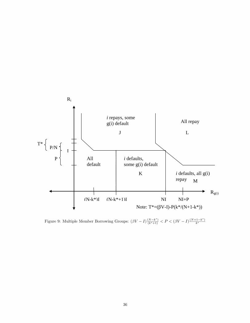
NI

I

NI+PRg(i)

Ri

Alldefault

i repays, someg(i) default All repay

i defaults,some g(i) default

i defaults, all g(i)repay

(N­k*)I (N­k*+1)I

J

K

L

M

P

P/NT*

Note: T*=(βV­I)­P(k*/(N+1­k*))

Figure 9: Multiple Member Borrowing Groups: (�V � I) (N�k�)

(k�+1) < P < (�V � I)(N+1�k�)

k�

36