1

Optimal integration of renewable based

processes for fuels and power production: Spain case study

Mariano Martín1a Ignacio E. Grossmann

b

aDepartment of Chemical Engineering. University of Salamanca. Plz. Caídos 1-5, 37008 Salamanca (Spain)

b

Department of Chemical Engineering. Carnegie Mellon University. Pittsburgh PA. 15213

Abstract.

In this work we propose a framework for the optimal integration of renewable sources of energy to

produce fuels and power. A network is formulated using surrogate models for various technologies that use

solar energy, photovoltaic, concentrated solar power or algae to produce oil, wind technology, biomass

based syngas to ethanol, methanol, FT-liquids and thermal energy, hydroelectric power and waste based

power plant via biogas production. The optimization model is formulated as an MILP that allows determining

the optimal selection of technologies to meet a certain demand; sustainability and CO2

Keywords: Wind power; Solar Energy; Biomass; Waste; Process integration; CO

emissions are also

considered. The network is applied to evaluate process integration at different scales, from province to

country level, and including uncertainty in sources availability. The solution suggests the use of hydropower

and oil production, while bioethanol and biodiesel plants are allocated close to fuel demand points such as

large population areas. Up to 20% of fuels and total power can be substituted with the current technology

and with 1% area usage. It is possible to reach 50% substitution with renewables using 20% area with the

availability and efficiency of current processes.

2

1 Corresponding author. Tel.: +34 923 294479. Email address: mariano.m3@usal.es

2

1. Introduction

Concern on global warming and the increasing demand for energy have increased the potential for

renewables to enter the energy mix. Among them, hydropower, wind, solar and biomass are the most

commonly used. While biomass is a raw material than can somehow be stored for a certain period of time,

and hydropower can be regulated [1], solar and wind energy are more difficult to handle [2]. Currently

battery systems do not have the capacity to store large amounts of power [3]. To meet a certain demand of

power and fuels, and mitigate the effect of the availability of renewable sources, several alternatives are

available such as thermal cycles [4], chemicals production, i.e. hydrogen or methane [5] or hydro-storage

[1]. Over the last years, plant integration of renewable resources has been considered for this purpose. First

and second generation bioethanol production processes were integrated [6] to make use of the excess of

energy when processing lignocellulosic biomass to provide energy for ethanol dehydration. Not only

biomass types, but different energy sources have also been integrated such as the facility that combines

solar concentrated power and biomass for maintaining the power production capacity over time [7]. Martín

and Davis [5] evaluate the integration of solar wind and power for the production of methane, synthetic

natural gas. Prasad et al. [8] evaluate the integration of solar and wind energy for power production to

mitigate the lack any of the sources. Martín and Grossmann [9] integrate solar, wind and biomass to capture

CO2, and hybrid systems are also presented in the recent literature [10]. The design of most of the facilities

involving renewables is subjected to the variability in the energy sources and that of the electricity price [2].

This variability affects the utilization of the units of the process, not only wind turbines and solar panels, but

also the number of electrolyzers in operation and process units. Some units may remain idle or partially idle

for certain periods of time representing an investment in units that is not used to their full capacity.

Therefore, resource variability determines the investment in expensive units. However, the design problem

involves multiperiod optimization under uncertainty. These kinds of problems have been addressed before in

the literature [11]. Grossmann and Sargent [12] included the uncertainty in the information within process

design. Later, Halemane and Grossmann [13] describe the problem of flexible process design. Both

concepts have regained attention with the inclusion of renewables in the energy mix. In the integration of

methanol via hydrolytic hydrogen and algae based oil [9], the problem is formulated in such a way that it

exploits the operation of the plant to reduce the problem size. Martín [14] present a methodology to address

3

the design and monthly operation of plants using renewable sources for the production of methanol from

CO2

However, large scale demand such as at regional or country level requires the integration of

resources at local or greater scale, a problem that represents a technical challenge [16]. Some studies

[17,18] present overviews regarding integration possibilities as a perspective for the combination of different

sources of energy. In order to help make those decisions, process system engineering has the tools to

compare sources, technologies and locations in search of the optimal use of natural resources for

renewable power and fuels production. Large scale integration of resources to control production capacity is

challenging due to the problem size and its mathematical complexity, together with the fact that that

renewables feature seasonal and daily variation. Most of the studies either focus on biofuels supply chain

design for different regions such as Europe [19], the US [20] or Canada [21], or electric power supply and

grid operation based on the unit commitment problem [22], considering market prices [23] even including

stochastic behavior of the variables [24], in particular applied to small regions [25]. In the case of the power

sector, heat is also typically included in the analysis [26]. However, electric power is most of the times

produced by using a fuel that may be synthesized such as methane or Fischer Tropsch fuels. Therefore,

both supply networks are linked and must be addressed simultaneously. So far both have been designed

independently due to the fact that they are areas that are studied by different communities.

hydrogenation. Surrogate models are developed, not only for the process units, but also for the cost of

the process sections so as to be able to include uncertainty in solar and wind into the design decisions.

Recent examples show the integration of hydro and photovoltaics [15].

In this work we extend the analysis of the generation of biofuels and power using renewable

sources by integrating the two networks that traditionally have been developed as independent entities.

However, they are linked by the common use of raw materials for the production of chemicals, fuels and

power as well as the possibility of storing power in the form of chemicals with the aim of meeting the

corresponding demands by making the most of the availability of different resources. In this sense, the

integration is more flexible since chemicals can be used to store energy as well as hydropower.

Furthermore, solar and wind variability are considered to evaluate the effect on the process integration. The

paper is organized as follows. Section 2 presents the technologies considered for the network. In section 3

we describe the model. We have divided the processes in subsections so that the intermediates can be

4

stored or used in various different processes such as syngas to hydrogen, ethanol or methanol. Section 4

presents results of the integration of renewables over time and under uncertainty, and the application of the

network in a multi area system so as to evaluate the production of power and fuels to meet the demand of

regions and countries. Finally, section 5 draws some conclusions.

2. Process network description.

We consider a large number of renewable raw materials including biomass, lignocellulosic and

waste, wind, solar and water. These sources are currently the basis for renewable based power and fuels in

most countries because of their availability and transformation capabilities. Lignocellulosic biomass can be

biochemically processed to bioethanol [27] or thermally transformed into syngas [28]. Syngas is a versatile

building block that can be further used to produce power, hydrogen [7], ethanol [28], synthetic Fischer

Tropsch (FT) liquids [29], methanol [9] or simply thermal energy [7]. Wind is used for power production [30],

and solar energy can be transformed into power using PV panels [31] or mirrors, using Concentrated Solar

Power (CSP) technologies. In this last case refrigeration systems are required and two alternatives are

typically evaluated, namely, wet [32] or dry [33] cooling. Power can also be produced using hydropower

facilities. When there is an excess of power produced, we can pump up water so that dams are used to

store power too in the form of potential energy. Furthermore, waste can also be used to produce biogas and

with it, power, using a gas and a steam turbine [34]. Alternative systems to store the excess of power

produced can be the production of hydrogen via water electrolysis, and with it, methanol [14] or methane

[30]. While methane can further be used in a gas turbine [34], methanol is used for oil transesterification in

the production of biodiesel. Algae are also grown consuming CO2

2.1.-Wind energy

, and with it, produce biodiesel [35]. As we

can see, renewables are fully interdependent and the integration is the natural step forward in the analysis.

In the following subsection we describe the processes that have proved to be promising in the

transformation of the above mentioned renewable raw materials into fuels, intermediate chemicals and

power based on previous work.

The electricity is generated in a wind farm, consisting of a number of turbines, as a function of the

wind velocity over time. The wind turbine investment costs are around 1500 €/kW [36].

5

2.2.-Solar energy

Solar photovoltaic panels are used to transform solar energy into power. The installation cost

ranges from 1,700 to 4,000 $ per kW installed [37], with a target of 1000 $/kW [38].

2.2.1.-PV solar

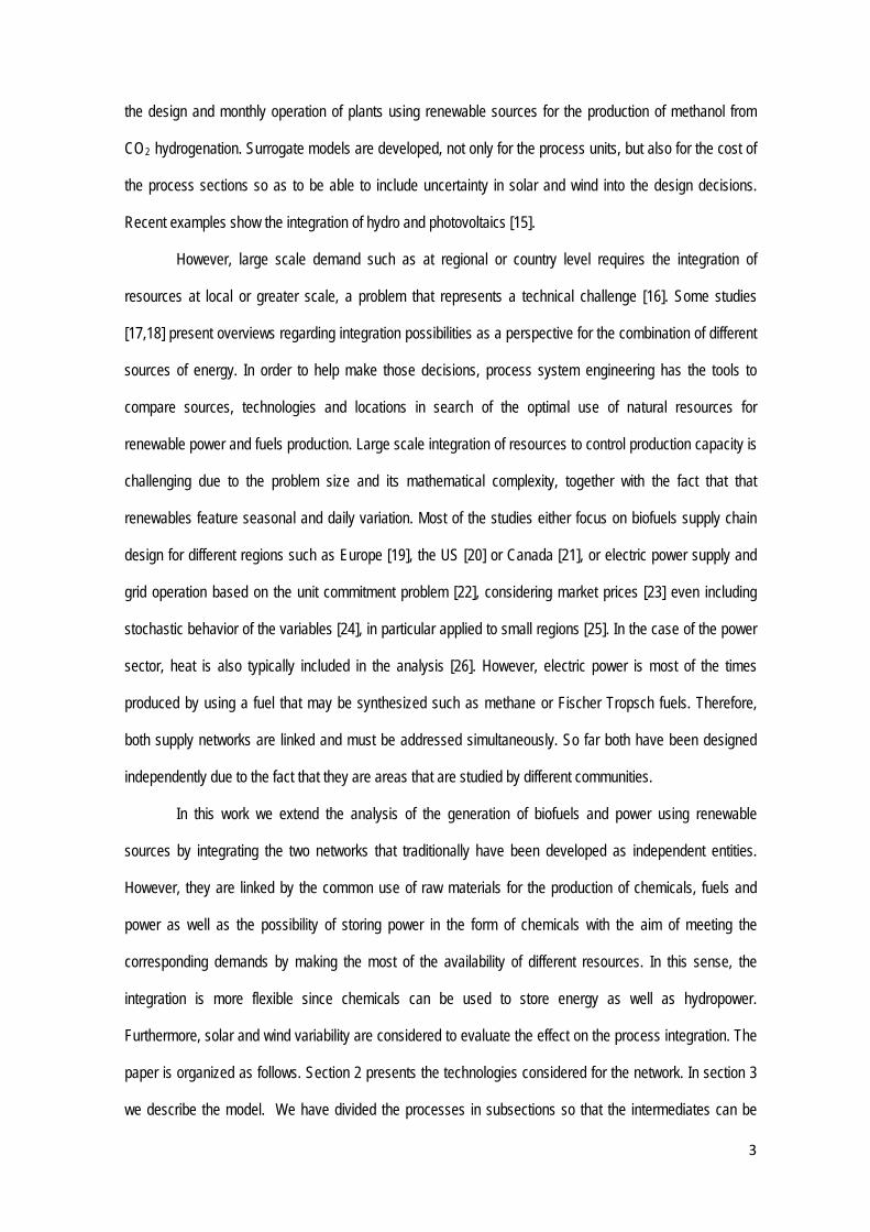
A CSP facility consists of three parts (see Figure 1): the heliostat field including the collector and

the molten salts storage tanks, the steam turbine, and the cooling system. The tower collects the solar

energy, heats up a transfer fluid, and produces steam for a regenerative Rankine cycle. The steam is

generated in a system of three heat exchangers where water is heated up to saturation, and then

evaporated using the total flow of molten salts. A fraction of the molten salts is used to superheat the steam

before it is fed to the first body of the turbine. The rest are used for the regenerative part of the Rankine

cycle. Both flows of salts are used to evaporate the water that has been condensed from the exhaust of the

turbine. In the second body of the turbine, part of the steam is extracted at medium pressure and is used to

heat up the condensate. The rest of the steam is finally expanded to an exhaust pressure, condensed and

recycled. We evaluate the use of cooling towers, whose operation requires water [32], or air cooler

condensers with an A-frame design [33].

2.2.2.-Concentrated Solar Power.

Special attention is paid to the cooling system. Either wet or dry cooling are common technologies.

The use of wet cooling consumes fresh water. When air coolers, typically A-frames, are used, a fraction of

the power produced is required to run the fans. The amount of power or water required to condense the

exhaust steam from the turbine depends on the ambient conditions.

6

Figure 1.- Concentrated solar power facility. HX: Heat Exchanger: CT: Cooling tower. HP: High pressure. MP: Medium pressure;

2.3.-Hydropower

Small-scale hydropower facilities are normally designed to use river flows, otherwise dams are built

to store water and use its potential energy to produce power. The idea is to couple the system with pumps

so that, if there is an excess of energy, water is accumulated at a high elevation to store energy in the form

of potential energy. The investment costs of large (>10 MWe) hydropower plants range from $1750/kWe to

$6250/kWe. It is very site-sensitive, with a typical figure of about $4000/kWe (US$ 2008). The investment

costs of small (1–10 MWe) and very small (≤1 MWe) hydro power plants (VSHP) may range from $2000 to

$7500/kWe and from $2500 to $10,000/kWe, respectively, with average costs of $4500/kWe and

$5000/kWe. Operation and maintenance (O&M) costs of hydropower are between 1.5% and 2.5% of

investment cost per year. The resulting overall generation cost is between $40 and $110/MWh (typical

$75/MWh) for large hydropower plants, between $45 and $120/MWh (typically, $83/MWh) for small plants,

and from $55 to $185/MWh ($90/MWh) for VSHPs [39].

7

2.4.-Biomass

Gasification of lignocellulosic biomass at high temperature, 850-1000 ºC, yields a mixture of

carbon monoxide and hydrogen, syngas, see Figure 2. Raw syngas is produced in the gasifier using steam

and oxygen as fluidification agents. Before further use, a train of clean up stages is required. First, it has to

be processed to remove hydrocarbons by means of a reforming stage using steam. Next, solids are to be

removed using either a scrubber or a filter system. Subsequently, its composition may need to be adjusted

for the proper H

2.4.1.-Lignocellulosic

2 to CO ratio, and finally sour gases, CO2 and H2

-The production of hydrogen is based on the well known water gas shift reaction where steam is

used to drive the equilibrium to the production of hydrogen. In situ recovery of hydrogen is possible using

membrane reactors [7]

S, must be removed to avoid catalyst

poisoning. Syngas is a very versatile raw material for producing chemicals such as hydrogen, methanol,

ethanol or more complex ones such as Fischer – Tropsch liquids.

2 2 2CO H O H CO+ → +

-The mechanism for producing methanol or ethanol is based on a Fischer-Tropsch type of

synthesis. The production of methanol is governed by the following set of reactions that take place at 200ºC

and 50 bar [9]. The purification of the products typically consists of the separation and recycle of the

unconverted gases and the dehydration of the methanol using a distillation column or molecular sieves.

2 2 2CO H O H CO+ → +

2 32CO H CH OH+ → -Ethanol production consists of allowing the carbon chain to grow a little further. Therefore, a part

from ethanol, methanol, propanol and butanol are also produced. The reactor operates at 300ºC and 68 bar,

where the desired reaction is shown below. After the recovery of the unreacted gases and its recycle, a

sequence of distillation columns is required to obtain flue grade ethanol [28]

2 2 5 22 4CO H C H OH H O+ → + -FT-Liquids production: The idea is to grow the carbon chain from the radical -CH2- by constantly

adding CO to the previous piece on the surface of the catalyst. The production of a particular chemical is

based on controlling the growth and the termination of the chain. Thus, diesel substitutes are typically

8

produced by operating the reactor at 30 bar and 212 ºC. The gas products can be used as fuel. Next, the

two-phase liquid mixture is separated to remove the aqueous phase, while the organic phase is sent to an

atmospheric distillation column. In order to increase the yield to fuels, the heavy components are broken

down using hydrocraking, and the mixture is fed to the same distillation column used for the separation of

the mixture obtained in the reactor [29].

2 2

2 2 2

2

2 ( ) ; H 165 /

n m

FT

mnCO n H C H nH O

CO H CH H O kJ mol

+ + → +

+ → − − + ∆ = −

The production of methanol, ethanol and FT-liquids generate thermal energy, but most importantly

in the case of FT-liquids, a flue gas is produced that can also be used to produce heat [40].

We can also use syngas directly as a fuel to produce thermal energy in a furnace or power, using a

gas turbine [7]. Figure 2 shows a block diagram of the process and the alternative uses of syngas. Further

information can be found in previous papers [7,9,28,29].

Figure 2.- Gasification based products diagram

Fermentation: Switchgrass is pretreated at 180 ºC and using a solution of 0.5% sulphuric acid in

water so that the structure of the grass is broken down. Next, enzymatic hydrolysis follows at 50ºC the pre-

treatment to obtain fermentable sugars, mainly xylose and glucose. Ethanol is obtained by fermentation of

the sugars at 38ºC under anaerobic conditions following the reactions below and reaching a concentration of

6-12% in water due to is poisonous effect in the enzymes.

5 10 5 2 2 5 22 + CO H=-74.986 kJ/molyeastC H O H O C H OH+ → ∆

6 12 6 2 5 22 + 2CO H=-84.394 kJ/molyeastC H O C H OH→ ∆

9

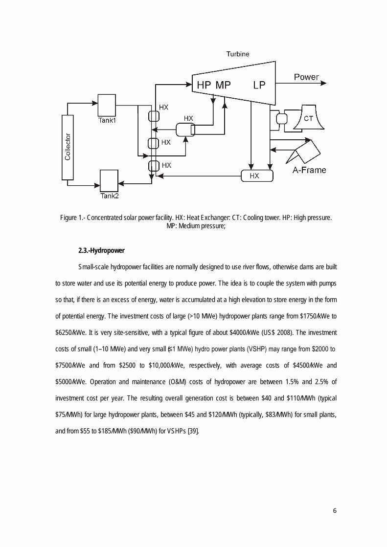
In order to reach fuel quality ethanol, water must be removed from the water-ethanol mix. A three

effect distillation column is used to remove most of the water before the final dehydration using molecular

sieves [27]. The lignin obtained as a byproduct is used to provide energy for the process and the excess can

be used within the network. Figure 3 shows the scheme of the process.

Figure 3.- Biochemical process to second generation bioethanol

Anaerobic digestion is a biological process performed by many classes of bacteria on a large

number of biomass types to produce biogas at 35-55ºC depending on the type of bacteria. The largest

biogas production yield takes place at 55ºC using thermophilic ones. The digestion as such consists of four

steps: hydrolysis, acidogenesis, acetogenesis, and methanogenesis. The actual biogas composition, from

50-70% in methane and 30-40% CO

2.4.2.-Waste: Biogas

2, with small amounts of N2, O2, H2S and NH3 depends on the raw

material, as well as the yield from biomass to biogas. The biogas must be cleaned from H2S and traces of

ammonia using adsorbent beds operating at 50ºC and 25ºC and 4.5 bar, respectively, before being used to

produce power. The CO2

present in the gas can also be removed using pressure wing adsorption (PSA) at

4.5 bar and 25ºC. The upgraded gas is used in a gas turbine. The high temperature of the exit gases make

them useful for the production of steam, and a steam turbine can be used to enhance the power production

of the facility [34]. The exhaust of the steam turbine must be cooled down. The same cooling technologies

as for the CSP plants can be used.

Algae are a rich raw material with a high yield compared to other biomass sources [41]. Its

composition as biomass consists basically of carbohydrates (starch), lipids, and proteins. There are a

number of options to grow the algae. We can distinguish between raceway ponds (circular, tanks,

paddlewheel raceways) or photo reactors (airlift, tubular, bag cultures). The first ones are simple civil

2.4.3.- Algae

10

engineering structures with small depth that are filled with water where the algae grow using CO2

or other

carbon source and nutrients [42]. The algae growth depends on the solar incidence and the carbon intake.

Another option is the use of photoreactors. The design of this equipment is more complex to allow solar

energy to reach the algae. Oil has to be extracted from the algae biomass. The extraction consists of the

use of mechanical action and solvents. The solvent is recovered using a distillation column and the oil sent

to the next stage. The production of biodiesel from oil is based on the transesterification reaction of the oil

with alcohols. The transesterification is an equilibrium reaction between the oil and alcohols. For economic

reasons, methanol has been used for a long time. From the technical point of view, it provides high yield to

biodiesel, fatty acid methyl ester (FAME), and quick reaction times. The excess of alcohol used to drive the

equilibrium to products is recovered in a distillation column whose bottoms operate below 150ºC to avoid

glycerol decomposition. If heterogeneous catalyst is used, no washing stage is needed, and a simple liquid

–liquid separator allows recovering the glycerol phase from the biodiesel phase. Biodiesel is purified in

another distillation column that operates under vacuum to avoid biodiesel decomposition, which occurs

above 250ºC. Figure 4 shows the block diagram from algae to biodiesel [35]

Figure 4.- Block diagram fro biodiesel production

2.5.-Chemicals from power

Electric power can be used to produce hydrogen, which is a promising energy carrier. It can also be

used to produce hydrocarbons from CO2. The process consists of an electrolyzer, an oxygen purification

section, a hydrogen processing section, and the synthesis part as seen in Fig 5. Both gas phases from the

electrolyzer must be dehydrated. The oxygen stream is cooled down to condense water at 25ºC. Next,

molecular sieves are used to dehydrate the stream before compression and storage. The hydrogen stream

also requires oxygen removal. A deoxo reactor operating at 90ºC is used, and the dehydration stage is

located downstream the deoxo reactor since it produces water. The hydrogen is now mixed with CO2 taking

in consideration that in order to avoid carbon deposition on the catalyst, a proper ratio of reactants is

11

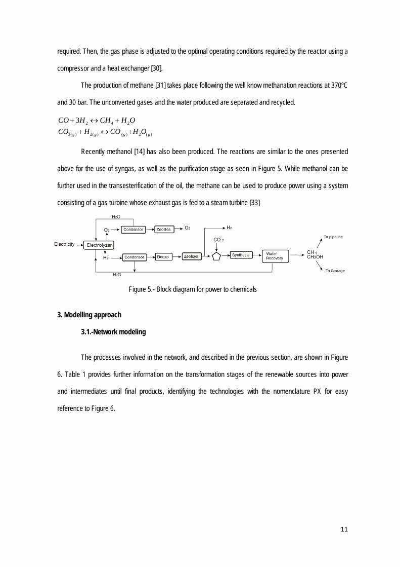
required. Then, the gas phase is adjusted to the optimal operating conditions required by the reactor using a

compressor and a heat exchanger [30].

The production of methane [31] takes place following the well know methanation reactions at 370ºC

and 30 bar. The unconverted gases and the water produced are separated and recycled.

2 4 23CO H CH H O+ ↔ + 2( ) 2( ) ( ) 2 ( )g g g gCO H CO H O+ ↔ +

Recently methanol [14] has also been produced. The reactions are similar to the ones presented

above for the use of syngas, as well as the purification stage as seen in Figure 5. While methanol can be

further used in the transesterification of the oil, the methane can be used to produce power using a system

consisting of a gas turbine whose exhaust gas is fed to a steam turbine [33]

Figure 5.- Block diagram for power to chemicals

3. Modelling approach

3.1.-Network modeling

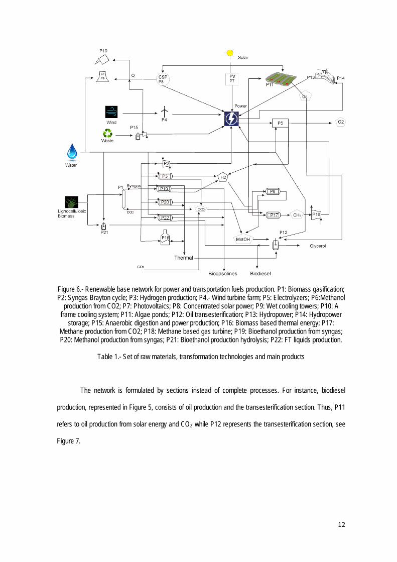
The processes involved in the network, and described in the previous section, are shown in Figure

6. Table 1 provides further information on the transformation stages of the renewable sources into power

and intermediates until final products, identifying the technologies with the nomenclature PX for easy

reference to Figure 6.

12

Figure 6.- Renewable base network for power and transportation fuels production. P1: Biomass gasification; P2: Syngas Brayton cycle; P3: Hydrogen production; P4.- Wind turbine farm; P5: Electrolyzers; P6:Methanol

production from CO2; P7: Photovoltaics; P8: Concentrated solar power; P9: Wet cooling towers; P10: A frame cooling system; P11: Algae ponds; P12: Oil transesterification; P13: Hydropower; P14: Hydropower

storage; P15: Anaerobic digestion and power production; P16: Biomass based thermal energy; P17: Methane production from CO2; P18: Methane based gas turbine; P19: Bioethanol production from syngas; P20: Methanol production from syngas; P21: Bioethanol production hydrolysis; P22: FT liquids production.

Table 1.- Set of raw materials, transformation technologies and main products

The network is formulated by sections instead of complete processes. For instance, biodiesel

production, represented in Figure 5, consists of oil production and the transesterification section. Thus, P11

refers to oil production from solar energy and CO2 while P12 represents the transesterification section, see

Figure 7.

13

Figure 7.- Modelling approach for process network development.

Each of the sections is modeled as black boxes considering inputs and outputs following the

principles in previous work [14]. For each of the sections a main input is identified. This variable, a mass or

an energy flow, has been used as the reference to compute the operation of that process, as well as the

production of a product, or a number of products, or the needs that are required for it to operate. The main

input for the different units is as follows: for wind, its velocity (m/s); for solar, the incidence (kWh/m2d), for

biomass, waste and water the flow in a period in kg or m3 per second available. Thus, the input -output black

box models are characterized by conversion and feed factors, Ki and Qi

{ }{ }

Pr ( , ) · ( , ) , , , ,

( , ) · ( , ) , ,i i

j i

od process t K In process t t i Raw materials Wind Solar Heat

Feed process t Q In process t t j Raw materials Heat

= ∀ ∈

= ∀ ∈

, which have been computed out of

detailed optimization models described in section 2. Revisiting our example in Figure 7, for P11, the main

input is solar energy and produces oil. Apart from the main input, any process also consumes other raw

materials or utilities. In the production of biodiesel, P12, apart from the main feed oil, the principal raw

material, methanol and thermal energy are also required. Thus, the sections models are written as follows:

(1)

The models of each one of the individual processes can be found in the supplementary material

along with the tables for coefficients Ki and Qi

( ) ( ) { }

( ) ( ) { }

genPower PowerP , , 2, 4,7,8,13,15,18

Power t PowerP , , 5,10,14process

useprocess

t process t t process

process t t process

= ∀ ∈

= ∀ ∈

∑

∑

. The aim of the network is to substitute power and fuels

demand. For the case of power, an energy balance accounts for the power generated by the various

technologies and that consumed internally, eq. (2)-(3). Note that the aim is not to use fossil based

resources, and therefore any power or thermal energy that the processes require must be produced

internally in the network and sometimes in the same spot such as the case of the need for thermal energy.

(2)

( ) ( )genPower t Power ( ) tuse t DemandP t− ≥ ∀ (3)

14

Power demand actually depends on the holiday periods and larger consumption is expected during

winter, December-January, July-August, and Easter. Thus, with respect to the annual average, we assume

the following normalized profile in the 12 months:

[1.1, 1, 0.9, 0.85, 0.95, 1, 1.1, 1.2, 1, 0.85, 0.9, 1.15].

The same profile is used for gasoline and diesel

The biogasoline produced corresponds to the production of ethanol via process P19 or P21 or the

green gasoline from the FT process, P22. However, since the energy content in ethanol is lower than that in

gasoline, we correct the production by a factor, γ, equal to 1.5, assuming the same density for both.

( ) ( ) ( ) ( ) ( )( )

( ) ( )

19

22

1Biogasoline _ prod Production P21, 1 ·Biomass _ use21 t Production P19, 1 ·Syngas

Production 22, 1 ·Syngas

P

P

t Out Out t

P Out t tγ

= +

+ ∀

(4)

Similarly, the renewable diesel produced is that obtained from biodiesel as well as that from the FT

process. However in this case the correction factor between diesel and biodiesel is almost 1, thus we

assume it to be 1.

( ) ( ) ( ) ( ) ( )22Biodiesel Production P12, 1 · t +Production 22, 2 ·Syngas tprod Puset Out Oil P Out t= ∀

(5)

Biodiesel requires thermal energy to operate. It has to be produced internally in the same province

as that where the transesterification takes place. There are some technologies that produce thermal energy

as byproduct, such as ethanol, methanol and FT fuels production, P19-P22, or we can produce it directly by

burning syngas, P16.

( ) ( ) ( )( ) ( ) ( )

ThermalE P12,t ThermalE P19,t ThermalE P20,t

ThermalE P16,t ThermalE P21,t ThermalE P22,t t

≤ + +

+ + ∀ (6)

Among the various products and intermediates, we allow storage of hydrogen, methane or

methanol. For the first month we do not assume any initial storage. From that point on, a mass balance at

each time period is formulated between the stock, the produced amount and the one used. We also assume

that the CO2, as a raw material, is either produced in the production of syngas or hydrogen from biomass, or

can be imported from a fossil source, CO2,fossil. The CO2

( )2, 2, 1 2, 3 2, 11 2, 17 2, 6CO +CO (t)+CO (t) CO (t)+CO (t)+CO (t) tFossil P P P P Pt ≥ ∀

is used to produce methanol or synthetic methane

via hydrogenation.

(7)

15

There is an area limitation for the installation of PV panels, mirrors and ponds. Initially we establish

it to be 1% of the area available. We assume that the turbines do not require this area. The complete model

is described in the supplementary material. Similarly, water consumption by processes must be available

locally. The complete model can be found in the supplementary material for reference.

3.2.-Cost correlations

The investment cost of each one of the processes or sections has been estimated using only the

units involved in the sections that have been selected. It is based on the units cost as described in previous

papers [28]. The units cost is estimated as a function of the mass or energy flow that they process. The

factorial method is used to compute the investment cost of the section of the facility. The method and the

correlations are found in [28].

The production cost of each section does not consider intermediates as a cost, since these costs

correspond to the sum of the production costs of each of the stages from the actual raw materials, biomass,

solar energy, wind energy, etc to the chemical. Thus, each section comprises the cost of operating that

section including utilities. Thermal energy is produced within the network. Since we need steam in most

cases, we still consider the cost of the steam since we need to transform the thermal energy generated into

the proper steam used at each stage

The process has to handle the largest of the flows over time. Thus, we define design variables that

will also determine the investment cost as follows:

( )FlowD tFlow t≥ ∀ (8)

For the cost correlations we have two types of models, linear and piecewise linear:

The only raw material that we actually pay for is biomass and it is assumed at a cost of $50/t. The

rest is produced internally, and the waste used to produce biogas, we provide treatment for it. Thus, the cost

for these sections, P1-P8, P10-P11, P13-P22 is given by eqs. (9)-(10). The coefficients in the equations can

be found in the supplementary material, Table 3S.

Linear correlations

CostInvest(Process)=αΙ ·DesignVar + βΙ YProc(Process); (9)

16

CostProd(Process,t)=αP · DesignVar(Flow) + βP

YProc(Process); (10)

For a number of facilities either the investment cost P9. P11, P16, P18, or both the investment and

the production costs, P12 & P19 are nonlinear. Therefore, a piecewise linear approximation is developed for

prespecified capacities, γ. Τhe cost correlations are then written as piecewise linear approximations as

given by eqs. (11)-(14). Table 4s in the supplementary material shows the discretization points.

Piecewise linear approximations

Variable in PrDesig n D ( )· ( );ocessγ

γ λ γ= ∑ (11)

Pr1 ( )ocessγ

λ γ= ∑ (12)

Pr

Pr

(1) (1)( ) ( 1) ( )

( ) 1

ocess P

ocess P P

P

YY Y

Yγ

λλ γ γ γ

γ

≤≤ − +

=∑ (13)

( ) PrCostP Process ( )·Cost ( ) ocess Eγ

λ γ γ= ∑ (14)

Further details of the cost correlations can be found in the supplementary material.

The objective function is that given by the operating cost, eq. (15). The production cost is given by

unit of time, thus, it is multiplied by the duration of the period, τ

Cost =

t

PrPr

13od t Invest

ocess tCost Costτ +∑ ∑ (15)

The model is extended to a network but applying it to particular regions in a geographic area. Thus,

each of the variables will have another index, the region. As a result, Eq. (15) is also extended to consider

transportation cost among regions. We consider distances computed from the longitude and latitude of the

allocations. Furthermore, variables accounting for the transportation of intermediates and products are

included. We consider that biogasoline, biodiesel, hydrogen, methane, oil, and methanol can be transported

at a given cost from one region to another in need. Power can also be transmitted, but we neglect its cost.

3.3.- Environmental metrics

3.3.1.-CO2

Apart from the economic objective function, we would like to evaluate the CO

mitigations

2 mitigation of each of

the networks to compare the effect of size and transportation on the CO2 emissions. We use eq. (16) to

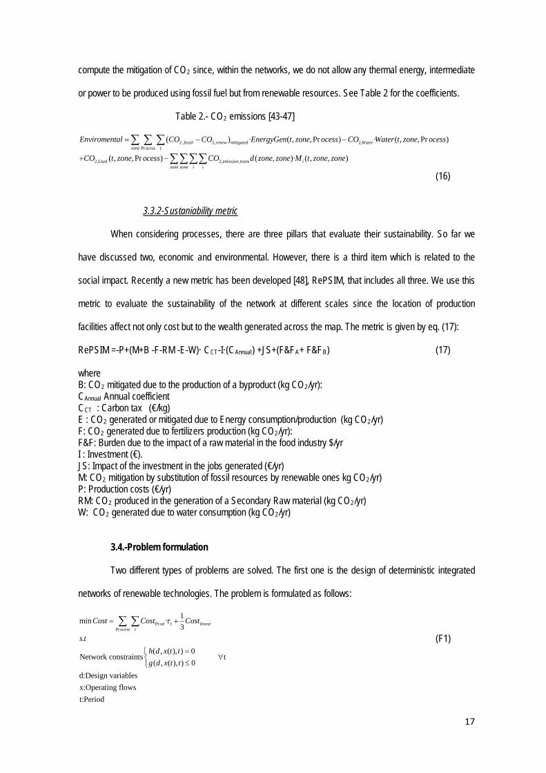
17

compute the mitigation of CO2

Table 2.- CO

since, within the networks, we do not allow any thermal energy, intermediate

or power to be produced using fossil fuel but from renewable resources. See Table 2 for the coefficients.

2

emissions [43-47]

2. 2, 2,Pr

2, 2, ,

( ) · ( , , Pr ) · ( , , Pr )

( , , Pr ) ( , )· ( , , )

fossil renew mitigated Waterzone ocess t

Used emission trans izo zone t i

Enviromental CO CO EnergyGen t zone ocess CO Water t zone ocess

CO t zone ocess CO d zone zone M t zone zone

= − −

+ −

∑ ∑ ∑

∑∑∑ne

∑

(16)

3.3.2-Sustaniability metric

When considering processes, there are three pillars that evaluate their sustainability. So far we

have discussed two, economic and environmental. However, there is a third item which is related to the

social impact. Recently a new metric has been developed [48], RePSIM, that includes all three. We use this

metric to evaluate the sustainability of the network at different scales since the location of production

facilities affect not only cost but to the wealth generated across the map. The metric is given by eq. (17):

RePSIM =-P+(M+B -F-RM -E-W)· CCT-I·(CAnnual) +JS+(F&FA+ F&FB

) (17)

where B: CO2 mitigated due to the production of a byproduct (kg CO2C

/yr): Annual

C Annual coefficient

CTE : CO

: Carbon tax (€/kg) 2 generated or mitigated due to Energy consumption/production (kg CO2

F: CO/yr)

2 generated due to fertilizers production (kg CO2F&F: Burden due to the impact of a raw material in the food industry $/yr

/yr):

I : Investment (€). JS: Impact of the investment in the jobs generated (€/yr) M: CO2 mitigation by substitution of fossil resources by renewable ones kg CO2P: Production costs (€/yr)

/yr)

RM: CO2 produced in the generation of a Secondary Raw material (kg CO2W: CO

/yr) 2 generated due to water consumption (kg CO2

/yr)

3.4.-Problem formulation

Two different types of problems are solved. The first one is the design of deterministic integrated

networks of renewable technologies. The problem is formulated as follows:

PrPr

1min ·3

.( , ( ), ) 0

Network constraints t( , ( ), ) 0

d:Design variablesx:Operating flowst:Period

od t Investocess t

Cost Cost Cost

s th d x t tg d x t t

τ= +

=∀ ≤

∑ ∑ (F1)

18

The constraints are the mass and energy balances modeling each of the processes as well as the

demand for fuels and power; see supplementary material. We use also as constraints the sustainability

metrics. This formulation (F1) is applied to a province, section 4.1, and then extended to two larger scales,

region and country level by including the transportation and transmission of fuels and power, (F1’), is applied

in section 4.3 where index i represents each one of the locations. Thus, the network model presented in the

supplementary material is applied to each one of the locations. Transportation of fuels and transmission of

power is included as a cost too.

PrPr

1min · o s ( , )· ( , )3

.( , , , ) 0

Network constraints ,( , ( ), , ) 0

Goods exchange : ( , ( ), ) 0d:Design variable

od t Invest Transportationj ocess t i

ij

Cost Cost Cost C t i j d i j

s th d x t i

t ig d x t t i

m d x t t

τ= + +

=∀ ≤

≤

∑ ∑ ∑ ∑

sx:Operating flowst:Period

(F1’)

Again, the constraints correspond to the mass and energy balances modelling each of the

processes; see supplementary material.

The second type of application is the extension of (F1) to the design of process networks under

uncertainty (F2). Solar, wind and demand are uncertain variables that affect the network design in terms of

selection of technologies and inventory. The problem is formulated as a two-stage stochastic optimization

problem (see section 4.2) where θs

PrPr

1min ( ) ( )·3

.( , ( ), , ) 0

Network constraints ,( , ( ), , ) 0

d:Design variablesx( ):Operating flow for scenario st:Period

:

Invest s od s ts ocess t

s s s

s s s

s

s

Cost Cost p Cost

s th d x t

t sg d x t

θ θ τ

θ θθ θ

θ

θ

= +

=∀ ≤

∑ ∑ ∑

Stochastic parameter for scenario s.

represents scenario s for uncertain parameter θ. For each of the

uncertain parameters, three scenarios are considered with low, medium and high probability. We apply the

formulation to the same province as F1 and only at province level for this case of study.

(F2)

We annualize the cost of the investment using 1/3 [49]. In this work we aim at process integration

and therefore a time period of months has been considered. Control and scheduling will be part of further

work.

19

4. Results and discussion

Data for the model does not only include process data, but also weather and demand data. The

total amount 251,749 millions of kWh is distributed per region as a function of the number of inhabitants [50].

The same is true for the consumption of fuels. Spain consumes around 632 kg/s of diesel and 124 kg/s of

gasoline [51] . We assume that 1% of the area can be devoted to solar panels, mirrors and/or ponds.

Lignocellulosic biomass is already there, either because it is the residue of the agricultural industry, or it

grows in the area. Water availability for hydroppower is based on assuming that the current capacity can be

expanded by 25% [52]. Typicaly the installed capacity is several times that produced regularly. That power

is available to be used and distributed in the different regions by the number of habitants. Wind is

determined from monthly maps [53]. Waste is computed by the amount generated per animal and the

census of the Spanish government [54] . Solar irradiation is from the AEMET atlas [55]. Biomass resources

are obtained considering three sources either forest residue [56], the straw that is not used by cattle [57] or

perennial miscanthus [58]. We assume that the availability is evently distributed over the year and over

provinces based on their area with respect to the region.

We divide the presentation of results into two levels. First province level, which aims at the

development of process integration for individual regions. We take advantage of the formulation and the

information available to compare the effect of uncertainty in the renewable resources, wind, solar and

biomass, in the evaluation of their use on the investment and the sustainability of the solution. The second

level shows interconection between provinces. In this case we compare two sizes, a region, since in Spain

these regions have their own government, and the entire country. This second set is evaluated only as a

deterministic problem where use use daverage values for wind velocities, solar and biomass availabilities.

The aim is to evaluate the scalability of the model and the advantages of a larger integration, as well as the

distribution in the use of resources when a more heterogeneous area, in terms of resources availability, is

considered. For instance, the South of Spain shows large solar availability while to the North, larger

lignocellulosic reserves are available.

20

4.1.- Province scale.

This section evaluates the integration of technologies so that a particular small region, a province,

operates on its own resources. In a second step, the effect of the uncertainty in the availability of the major

renewable resources on the selection of technologies and the installation cost is considered. Note that

biomass availability and its cost are not independent. Therefore, we use biomass variability as uncertain

variable together with solar and wind availability and power demand.

4.1.1.- Optimal deterministic multiperiod process integration.

We select one location with the characteristics shown in Table 3. Electricity is estimated by the total

power requried per inhabitant and the people living in that region. We assume that power, gasoline

susbtitution and diesel substitution changes throughrout the year depending on the holidays period as

presented above and the weather. For instance, a larger amount of fuels is requried in summer due to

holiday season as well as in winter, because of the weather. We use the trends of Spain for that since the

solar and wind velocities correspond to allocations in the South of Spain.

We apply the network to analyze the province level in Almeria in order to determine the optimal

integration of renewable technologies to meet the electricity demand, and cover 20% of the gasoline and

diesel demand of the local population over 12 time periods (months). The problem size of the multiperiod

MILP is 1269 eqs. 985 var and 54 discrete variables. It was solved in less than 1 CPU min with CPLEX 12.6,

in an Intel core i7 machine running Windows 10. Table 3 shows the main weather data for this location.

Table 3.- Input data for process integration

The renewable based network of technologies consists of 100 turbines and electrolyzers as well as

16551 ponds. We require 2.9 ·106 m2 of area for PV panels and 1.6107 m2 is used by the ponds. Electric

power is produced using solar energy, PV panels, and wind turbines. Part of the power is used to produce

hydrogen that is intended to produce the methanol needed for the transesterification of the oil. Diesel

susbtitutes are only produced using this technology Thermal energy is also required to produce biodiesel.

This type of energy is either produced together with ethanol from biomass via hydrolysis, or directly by

burning biosyngas. By using this network 2.8 t/s CO2 are avoided by the susbtitution of the fossil sources

for electricity and fuels by renewables ones. The environmental metric reports a positive value of 3.8 ·10 8

21

€/y. The high demand of diesel and its direct dependence on solar energy, results in the need to store oil

along the year to be used during winter (see Figure 8). Figure 9 shows the consumption of water and CO2

from fossil source used by the network over time. The investment required for the optimal economic solution

is 3.4 billion €.

Figure 8.- Availability of stored chemicals over time

Figure 9.- Use of utilities and materials

4.1.2.- Optimal stochastic multiperiod process integration.

For the same province, Almería, we solve a two-stage stochastic programming model considering

that power demand, solar, biomass and wind availability are uncertain. Note that biomass cost is directly

related to its price. Therefore we do not consider biomass price as uncertain. For each of the parameters we

consider three scenarios with a probability of low, medium and high. 81 scenarios per month are considered

22

for the 4 uncertain parameters. The aim is to determine the optimal integration of renewable technologies to

meet the electricity demand, and cover 20% of the gasoline and diesel demand of the local population over

12 months . The problem size of the MILP formulation is 90,527 eqs. 66,265 var and 54 discrete variables

that was solved with CPLEX 12.6, in an Intel core i7 machine running Windows 10, requiring 10 min CPU

time.

We require 100 electrolyzers, 100 wind turbines and 18505 ponds. 4.17·106 m2 of solar PV panels

and the rest of the area is used by the ponds. Figures 10 and 11 summarize the monthly average operation.

Oil is stored over time so as to produce biodiesel for the months that have lower solar incidence. Process

water consumption as well as biomass are consumed regularly, while CO2

is mostly consumed during the

first months of the year to produce the oil that is stored, and its consumption decreases by the end of the

period. Compared to the deterministic solution, there is a larger investment of 4.0 billion €, so as to have

flexiblility in the operation. This is the result of the additional production of hydrogen from biomass and the

addition of hydropower as well as the production of methane to be stored as a mean to store the punctual

excess of power. Finally, the substitution of fuels is performed with bioethanol via hydrolysis of biomass and

algae based, as well as with biomass based FT fuels.

Figure 10.- Availability of stored chemicals over time under uncertainty

23

Figure 11.- Use of utilities and materials under uncertainty

This sistem is not only more robust, but it also shows larger positive RepSIM value of 4.0·108 vs

3.8·108 €/y . However, there is a slight reduction in the CO2 mitigated, 2.7t/y of CO2

4.2.-Multiregional integration.

vs 2.8t/y in the previous

case, due to the duplication of technologies. In terms of the technologies selected, the system does not use

biosyngas to produce power, but it produces hydrogen that is accumulated as a buffer.

In this section we evaluate two integration levels deterministically, regional and national, in order to

show the changes in the selection of technologies when a more integrated plan is in place, as well as to

present how the problem scales in our attempt to reach the European level.

4.2.1.-Small region (Andalucía)

The further step is to apply the model to a region of several provinces. We select Andalucía. It

consists of 8 provinces, including the one used as individual case study above, Almería. It is located at the

South end of Spain and it is characterized by high solar energy availability, and a couple of regions such as

Almería and Cádiz, with high wind velocity. The idea is to apply the model of the network for each of the

regions and determine transfer of intermediates and final products so as to meet the demand of each region.

We add transportation costs for the liquids and gases based on the distance between every two locations.

24

Power, on the other hand, is assumed to be transmitted with no loss for free. In principle all the transfers are

available, and the cost is based on the distance and the amount shipped will define which ones to use.

Again, we determine the optimal integration of renewable technologies to meet the electricity

demand and cover 20% of the gasoline and diesel request of the local population. The problem size

becomes 15,043 eqs. 18,795 var and 432 discrete variables and was solved with CPLEX 12.6, in an Intel

core i7 machine running Windows 10, requiring 1min CPU time. The technologies selected to meet the

power demand and to reach 20% fuel substitution, are presented in Figure 12. Each symbol represents a

facility of a corresponding technology. Only the number of panels, ponds or the wind turbines are

represented with one symbol for whichever number is required. The actual numbers are commented in the

text for simplicity of the figure. The substitution of fossil based fuel and energy by renewable sources results

in enviromental disadvantages with respect to the province level, reporting a lower value in CO2 mitigation,

2t/s, mainly due to tranport. Furthermore, the RePSIM metric shows a positive value, 4.0·109

Hydropower is selected for all locations, providing a technology to store the excess of power when

needed. Ethanol is produced from biomass hydrolysis in all the provinces except for province 7. This facility

also produces thermal energy that is required for biodiesel production. Methanol is produced is the same

provinces as those that produce biodiesel since it is requried for oil transesterification, and transport is not

recommended due to its cost. Only Huelva, province 5, does not produce biodiesel but it produces oil. Solar

energy is used in the southeast, provinces 1 and 4, Almería and Cádiz, and only province 1 is selected for

the installation of a wind farm of 100 wind turbines. As a result, the major producers of power are these two

regions, see Figure 12. Biodiesel and biogasolines production is quite distributed, and most of the regions

produce a fair amount of products reducing the transportation needs. Even though the production is

distributed, provinces 2, 8 and 7 are the major producers of biodiesel.

€/y. The

investment required to establish such a network over the 8 provinces region adds up to 40 billion €.

25

Figure 12.- Allocation of technologies in a region

1:Almería;2: Cádiz; 3: Córdoba; 4: Granada; 5: Huelva; 6: Jaén, 7: Málaga; 8: Sevilla. The full profiles of the production of biodiesel, biogasolines power, methanol hydrogen and water

can be seen in Figure 13. The production of liquid fuels is quite steady over time. Only a certain degree of

oscillation can be seen in provinces 1,5 and 6 in the case of biodiesel. In the case of biogasolines

susbtitutes, it is not that constant and we can see how provinces 2 and 1 & 6 are opposite in the production

profiles showing a large profile in summer in Cadiz, province 2, while provinces 1 and 6 reduce their

production over these months. In case of power, province 4 is the major producer and focusses its

production over summer so that is mostly resposible for all power production. Province 1 complements

region 4 during winter time. We see that the production of hydrogen and methane reaches a steady state

from May onwards, actually, the storage of energy in the form of these two is quite obvious.

26

Figure 13.-Operation of the network. 1:Almería;2: Cádiz; 3: Córdoba; 4: Granada; 5: Huelva; 6: Jaén, 7: Málaga; 8: Sevilla.

The distributed production shown reduces the transportation of goods as seen in Figure 14. During

the first month of the operation, there is quite a few transports of goods, mostly power, but also

biogasolines. Province 7 recieves gasoline. As it can be seen, typically province 7 is a net importer of

gasoline over the year. Power is transferred from 1 and 4 to reach three where it is distributed. This pattern,

as well as that of biogasoline, is common along the year; see April, July and October as representatitve

months of the various seasons. The transported goods decrease over the year, see April. Solar energy

increases allowing larger production of biodiesel and power. The increased demand during summer, see

July as an example month, also increases the transport of gasoline, while fall is characterized by power,

hydrogen as power storage, and a small ammount of biogasoline transport.

27

Figure 14.- Flows of mass and power in Andalucía (Black: Power ; Red: H2

1:Almería;2: Cádiz; 3: Córdoba; 4: Granada; 5: Huelva; 6: Jaén, 7: Málaga; 8: Sevilla.

, Green: Methanol, Blue Gasoline, Biodiesel: Brown)

4.2.2.-Country scale case of study: Spain.

Finally, we apply the optimal renewable based technology selection to the entire country, Spain.

The same assumptions as for the smaller region still hold, as well as the source for the data. A total of 47

provinces are selected in the peninsular area. Again, we determine the optimal integration of renewable

technologies to meet the electricity demand, and cover 20% of the gasoline and diesel demand. The

problem size for the deterministic case becomes 240,596 eqs. 419,478 var and 2,538 discrete variables. It

was solved with CPLEX12.6, in an Intel core i7 machine running Windows 10, requiring 25 min. We focus on

minimizing the cost, but we also include results on the sustainability of the network. Figure 15 shows the

optimal distribution of technologies across Spain for meeting the power demand, and reaching 20% of the

fuels substitution. As in the case of the smaller region, each symbol represents a facility of the

corresponding technology. Again, only the number of panels, ponds or the wind turbines are represented

28

with one symbol for whichever number is required. The actual numbers are commented in the text for

simplicity of the figure.

The first comparison is with the smaller region presented in section 4.2.1, see Figures 12 and 15. It

can be seen that the solution spreads the use of resources reducing the concentration of technologies in

provinces such as 1,3,4,5. Bioethanol is no longer produced in almost all provinces. At the national level,

biogasolines are no longer produced only using biomass hydrolysis, but gasification also plays a role for the

production of not only bioethanol, but also methanol. At any scale, hydropower is recommended, but at

national level no methane is used to store power. Biodiesel is no longer produced in provinces 1,3,4 since

larger production centers are suggested at the national level. Comparing the south region in Figure 12 with

Figure 15, we also identify other differences in the selection of technologies. For instance, solar energy is

more widely used when the national scale is analyzed and provinces 1,2,4,6-8 use PV , together with 17 and

19. In the case when evaluating Andalucía alone, only province 1 uses PV panels. The reason may be the

need to meet the demand of biodiesel since ponds already use a large area.

At the national level, areas of more concentrated use of technologies correspond to those with

higher demand such as Madrid, Barcelona, Seville, Vasque Country and the Mediterranean coast, mostly to

reduce transportation. Analyzing in more detail the solution at the national level, we start by the substution of

gasoline. Gasoline substituttion is mostly accomplished by bioethanol produced from hydrolisys of biomass.

Provinces that produce ethanol via hydrolysis are 3,4,11-12, 21,27,30,34-37, and 42. As it can be seen in

Figure 16, the major producers of biogasoline subtitutes are provinces,12, 13. A number of provinces

produce between 2 and 3 kg/s of substitutes, in all cases these are typical facilities sizes in the biofuels

industry. Most of the provinces produce a small amount, almost for self production. Gasification based

ethanol is only used in a few provinces such as 2,7, 10, 23, 41, 46,47. The provinces rarely coincide with the

ones that produce biodiesel. Provinces 2, 7 and 37 produce both ethanol and biodiesel even though ethanol

is produced via hydrolysis in province 37 and via gasification in the other two. Biodiesel is produced across

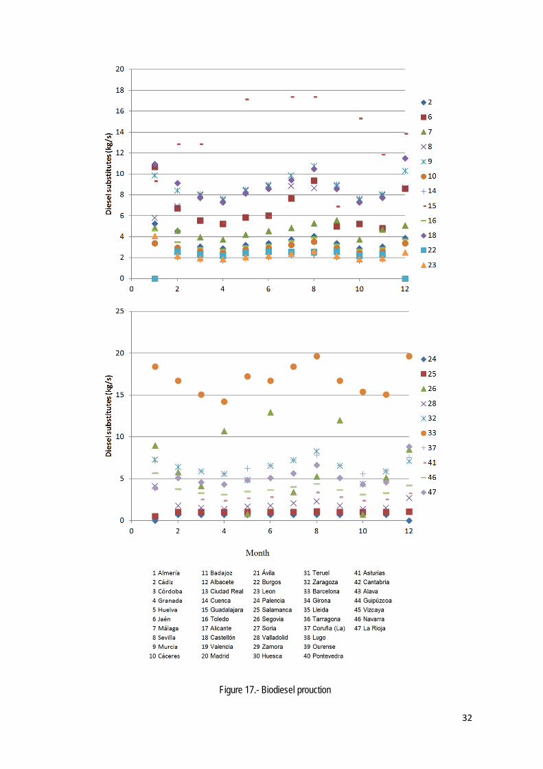
the territory in provinces such as 2,6,7,8,9,10,15,16,18,23, 25,26,32,33,37,41,46,47. In Figure 17 we see

that the major producers of biodiesel are provinces 15, 26 and 33. We can also see that medium size

facilities, producing from 2 to 9 kg/s follow the profile of the demand, with an increase in the production

during summer. The pattern corresponds to the possibility of serving it across the country, but close to the

29

centers of larger consumption. Oil is locally produced in the same provinces as biodiesel, as well as

methanol. Only few locations at the coast, provinces 20, 21 30, 35 and 38 produce oil on its own. Taking a

closer look, these provinces as situated in between provinces that produce biodiesel. Since biodiesel

requires thermal energy, typically biomass is also used to produce the thermal energy required in the same

province. FT liquids production can se seen in provinces 6,9, 14,16, 22, 24 and 33. These regions produce

mostly biodiesel substitutes but a small amount of gasoline as byproduct of the FT process.

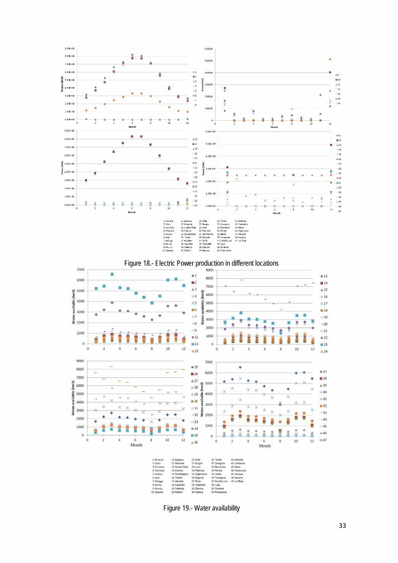
Figure 18 shows the production of power. We see that it follows the seasonality and it is focused on

a few provinces such as 1,2,4, 17 and 19, corresponding to the ones with large solar availability. For the

provinces that produce electric power using wind turbines, 100 wind turbines are installed at each one of the

locations selected for that technology. The Mediterranean coast and the center of the peninsula use wind as

power source. Note that wind turbines are already installed in central Spain, somehow validating the results

obtained by the model. In the case of solar panels, as presented above in comparison with a smaller size

region analysis, provinces 1,2,4,6-8 use PV. In all cases the area available for them is used. Note that the

area available is distributed between ponds, panels and mirrors. In terms of ponds, there are only three

locations producing oil that do not use the maximun number of 50000 ponds, 2, 7 and 17. Water availability

is quite regular in all provinces, with minimum in summer and maximum in March, see Figure 19. With large

availability we can find only a few ones, 10,11, 23, 20, 20, 32, 33, 37 and 40. However, the possibility of

storing energy using dams, suggest the use of hydropower plants all over the territory.

30

Figure 15.- Allocation of technologies across Spain

31

Figure 16.- Biogasolines production

32

Figure 17.- Biodiesel prouction

33

Figure 18.- Electric Power production in different locations

Figure 19.- Water availability

34

The investment for the network becomes 189 billlion euros. Since dams are already built in Spain ,

hydropower could have eliminated them from the cost. However, for us to decide on the best integration, we

decided to consider decisions from grassroots. In terms of enviromental comparison with previous cases we

see that while the RepSIM value is positive, 1.9 ·1010 €/y and higher than before, CO2 is actually mitigated

1.2·105 kg CO2

/s, even considering the transportation of fuels.

If we go a step forward, with the current yields of the biomass and the technologies, it is not

possible to reach full substitution of biofuels. Therefore, we call here for a more efficient growth of biomass

so as to reach the goal of full renewable plants, as well as the need to further integration with Europe.

Another important consideration is the use of cars and their efficiency. Recent trend of hybrid or electric

cars, at least for urban areas, can help reach full renewable fuels and power systems. Thus, we focus on

reaching 50% by using 10% area for ponds and solar capturing devices (PV panels and mirrors). Figure 20

shows the selection of technologies for 50% liquid fuel substitution. The first thing to note is the fact that the

solution is not incremental with respect to the previous one. Apart from the fact that there are a larger

number of production facilities using a biochemical path to ethanol, it is important to mention that solar

energy is reduced to only province 7, since the area is required for biodiesel production in ponds. This

means that to increase the production of fuels is not that we add a few more biofuel production facilities, but

a new production system is required. The production of biodiesel results in the fact that typically in the same

province, oil, methanol and thermal energy are produced, since all are required to obtain biodiesel.

However, apart from the provinces that produce biodiesel in both scenarios, 20% and 50% fuel substitution,

some provinces change the production scheme from biodiesel to bioethanol when a larger fuel substitution

is required, i.e. province 25 or 46, or on the other direction, province 3 abandon bioethanol production to

focus on biodiesel. Some others incorporate facilities to produce both types of substitutes. It is also true that

there is a common structure, such as the need for hydropower across the territory and the use of wind

power in the same provinces as the previous scenario. Therefore, the substitution of fossil based fuel and

power has to be carried out following a strategic plan over time. Actually, the cost to reach 50% liquid fuels

substitution only represents an increase of 1% higher cost that the base case scenario, 192B€. The

sustainability of the solution is similar, in terms of the use of the RepSIM metric, 1.9 ·1010 . However, the

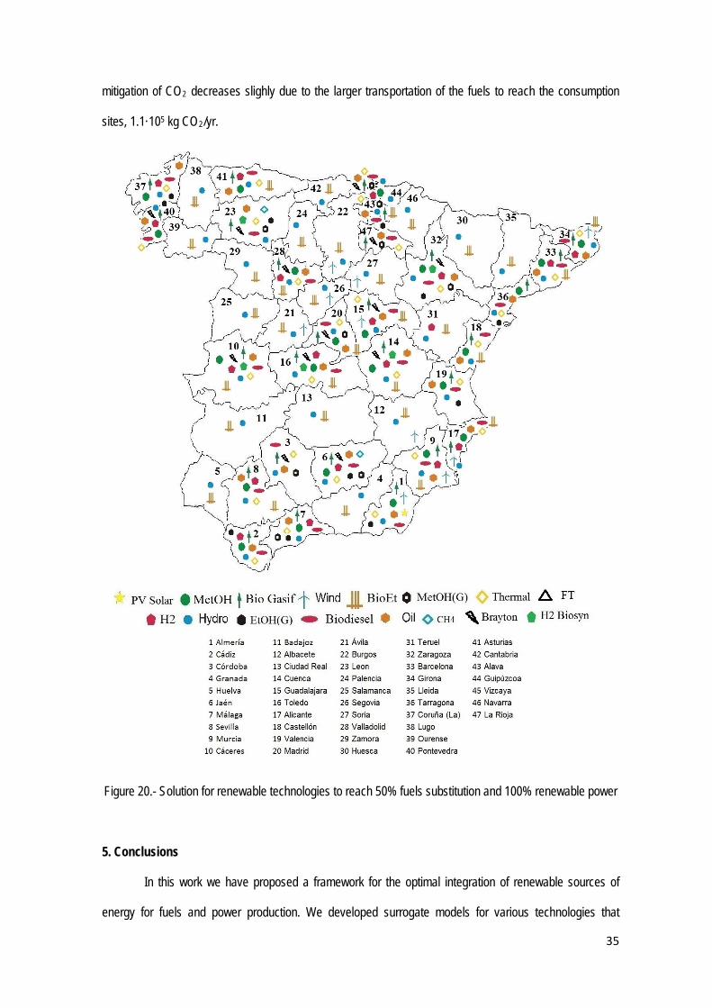
35

mitigation of CO2 decreases slighly due to the larger transportation of the fuels to reach the consumption

sites, 1.1·105 kg CO2

/yr.

Figure 20.- Solution for renewable technologies to reach 50% fuels substitution and 100% renewable power

5. Conclusions

In this work we have proposed a framework for the optimal integration of renewable sources of

energy for fuels and power production. We developed surrogate models for various technologies that

36

include solar energy, PV solar, CSP or algae to produce oil, wind technology, biomass based syngas to

ethanol, methanol, FT-liquids and thermal energy, hydroelectric power and waste based power plant via

biogas production. The deterministic and the two-stage stochastic programming models allow determining

the optimal selection of technologies to meet certain demand. Cost objective functions and environmental

metrics are used.

We have evaluated the integration in a small region (Almería) and added the effect of the

uncertainty in the availability of solar, wind, biomass and power demand on the solution. As expected, the

solution under uncertainty yields higher cost, but it yielded a more robust operation by using a larger number

of energy sources. Later, we extended the application to a region, Andalucía, and to an entire county, Spain.

The results for the deterministic cases show that for a region the technologies are concentrated, and most of

the areas require most of the technologies. However, if a larger area is considered, the technologies are in

general more spread out. Concentration of technologies can be found in the areas with larger demand, big

cities such as Madrid, Barcelona, Bilbao and Seville. The substitution of fossil based fuels and power is

limited by the resources available. It is possible to reach 50% substitution of fossil fuels by using 10% area,

but the limitations in biomass availability prevent achieving complete substitution of fossil fuels.

The proposed framework can easily be applied to any other regions, providing a tool to evaluate

the use of renewable resources and provide informed decisions on how to locate technologies from a certain

basis.

6. Nomenclature

Ai: Area of unit i (m2

A)

Region: Area of the zone evaluated (m2

B: CO)

2 mitigated due to the production of a byproduct (kg CO2Biodiesel

/yr): prod

Biomass_av(t): Available biomass in a month (kg/s) (t): Biodiesel produced in period in a particular zone (kg/s)

Biomass_usePBiogasoline_prod(t): Renewable substitutes of gasoline in process (kg/s)

: Consumption of biomass in period by process P (kg/s)

CAnnualC

Annual coefficient CT

CH4 : Carbon tax (€/kg)

PCO

(t): Methane produced in period (kg/s) 2fossil(t): Flow of CO2

CO from fossil fuels used (kg/s)

2P (t): Flow of CO2Cost

used or produced in process P (kg/s) E

Cost: Fixed parameter of cost for the piecewise linear approximation (MM€ or MM€/y)

InvestCost

: Investment cost (MM€) Prod

E : CO: Production costs (MM€/s)

2 generated or mitigated due to Energy consumption/production (kg CO2/yr)

37

F: CO2 generated due to fertilizers production (kg CO2F&F: Burden due to the impact of a raw material in the food industry $/yr

/yr):

H2availableH2

: Hydrogen available in a region (kg/s) electro

H2: Hydrogen produced in a single electrolyzer (kg/s)

PI : Investment (€).

: Flow of H2 used or produced in prices P (kg/s)

JS: Impact of the investment in the jobs generated (€/yr) M: CO2 mitigation by substitution of fossil resources by renewable ones kg CO2MetOH(t): Methanol produced in a zone in period (kg/s)

/yr)

MetOHavailNPond

(t): Methanol available in a zone in period (kg/s) Desing

N: Number of ponds in a zone to be built

turbineN

: Number f wind turbines in a zone to be installed electro:

O2Number of electrolyzers in a zone to be installed

POil

: Oxygen produced in electrolysis (kg/s) Prod

P: Production costs (€/yr) (t): Oil produced in a particular region in period (kg/s)

PowergenPower

(t): Power generated in the network in period (kW) use

PowerP(t, process): Power produced or consumed by process in period (kW) (t ): Power used by the network in period (kW)

QPRepSIM: Renewable metric (€/y)

(t): Cooling required by process p in period (kW)

RM: CO2 produced in the generation of a Secondary Raw material (kg CO2Solar (t) Solar incidence (kWh/m

/yr) 2

Syngas(t): Syngas produced (kg/s) d)

SyngasProcrsst: Period (month)

(t): Syngas consumed by process in period (kg/s)

ThermalE(per, Process) : Thermal energy produced or consumed in period by process (kW) W: CO2 generated due to water consumption (kg CO2Waste

/yr) in

Waste(t) : Consumption of waste in period (kg/s)

availWater(t, Process) : Water consumed in period by process (kg/s)

(t) : Waste available in period (kg/s)

WateravailxxxD=Desing

(t, Process) : Water available in period (kg/s) Variable

Yproc(process): Binary variable for the existence of a process : Design variable for a particular process.

YPZ: Objective function (€/s)

: Binary variable for the piecewise linear approximation

ε: Small parameter λProcess

: Variable for piecewise linear approximation

Acknowledgement

The authors appreciate Salamanca Research for software licenses and CAPD center for funding.

7. References [1] Rogeau A, Girard R, Kariniotakis G A generig GIS – based method for small Pumped hydro energy storage (PHES) potential evaluation at large scale. Applied Energy 2017; 197: 241-253 [2] Pfenninger S Dealing with multiple decades of hourly wind and PV time series in energy models: A comparison of methods to reduced time resolution and the planning implications of interannual variability. Applied energy 2017; 197: 1-13

38

[3] de Oliveira e Silva G, Hendrick P Photovoltaic self-sufficiency of Belgia households using lithium-ion battries and its impact on the grid Applied Energy 2017; 195: 786-799 [4] Takasu H, Ryu J, Kato Y Applicantion of lithium orthosilicate for high-temperature thermochemicl energy storage Applien energy 2017; 193: 74-83 [5] Martín M, Davis W. Integration of wind, solar and biomass over a year for the constant production of CH4 from CO2

and water Comp Chem Eng. 2015; 84: 314-25.

[6] Cucek L, Martín M, Kravanja Z, Grossmann IE. Integration of Process Technologies for the Simultaneous Production of fuel Ethanol and food from Corn grain and stover. Comp. Chem. Eng. 2011; 35(8): 1547-1557 [7] Vidal M, Martín M. Optimal coupling of biomass and solar energy for the production of electricity and chemicals.Comp. Chem. Eng. 2015; 72: 273-83 [8] Prasad AA, Taylor RA, KayM Assessment of solar and wind resource synergy in Australia. Applied energy 2017; 190: 354-367 [9] Martín M, Grossmann IE. Optimal integration of a self sustained algae based facility with solar and/or wind energy J Clean Prod. 2017; 145 (1): 336-347 [10] Forman, C., Gootz M, Wolferdorf C, Meyer B (2017) Coupling power generation with syngas-based chemical synthesis. Applied Energy 2017; 198: 180–191 [11] Grossmann IE, Apap RM, Calfa BA, García –Herreros P, Zhang Q. ecent advances in mathematical programming techniques for the optimization of process systems under uncertainty. Comp. Aided. Chem Eng 2015; 37: 1-14 [12] Grossmann IE, Sargent RWH Optimum Design of Chemical Plants with Uncertain Parameters, AIChE J. 1978; 24 (6): 1021-8 [13] Halemane KP, Grossmann IE.Optimal process design under uncertainty AIChE, J. 1983; 29 (3): 425-33 [14] Martín M. Methodology for solar and wind energy chemical storage facilities design under uncertainty: Methanol production from CO2

and hydrogen. Comp Chem Eng. 2016; 92: 43-54

[15] Jurasz J, Ciapala B Integrating photovoltaics into energy systems by using a run-off-river power plant with pondage to smooth energy exchange with the power grid. Applied Energy 2017; 198: 21-35 [16] Armendáriz M, Heleno M, Cardoso G, Mashayekh S, Stadler M., Nordström L. (2017) Coordinated microgrid investment and planning process considering the system operator Applied Energy 200:132-40 [17] Weekman VW. Gazing into an energy crystal ball. CEP June 2010; 23-27 [18] Yuan Z, Chen B. Process Synthesis for Addressing the Sustainable Energy Systems and Environmental Issues. AIChE J. 2012; 58 (11): 3370-89 [19] Cucek L, Martín M, Grossmann IE, Kravanja Z. Large-Scale Biorefinery Supply Network – Case Study of the European Union. Comp. Aid. Chem. Eng. 2014; 33: 319-24. [20] Elia JA, Baliban RC, Floudas CA.Nationwide energy supply chain analysis for hybrid feedstock processes with significant CO2 emissions reduction. AIChE J. 2012; 58 (7): 2142-54.

39

[21] Gautan S, Lebel L, Carle MA. Supply chain model to assess the feasibility of incorporating a termical between forests and biorefineries. Applied Energy 2017; 198: 377-384 [22] Saravanan B, Da S, Sikri S, Kpothari DP.A solution to the unit commitment problem-a review. Frontiers in Energy. 2013; 7(2): 223-36 [23] Dowling AW, Kumar R, Zavala VM A multi-scale optimization framework for electricity market participation. Applied energy 2017; 190: 147-164 [24] Papavasiliou A, Oren SSA stochastic unit commitment model for integrating renewable supply and demand response. IEEE. 2012. 978-1-4673-2729-9/12 [25] Nikmehr N, Najafi-Ravadanegh S, Khodaei A Probabilistic optimal scheduling of networked microgrids considering time-based demand response programs under uncertainty Applied Energy 2017; 198; 267-279

[26] Chen Y, Fei W, Liu F, Mei S (2017) A multilateral trading model for coupled gas-heat-power energy networks. Applied. Energy 200 180-91

[27] Martín M, Grossmann IE Energy optimization of lignocellulosic bioethanol production via Hydrolysis of Switchgrass. AIChE J. 2012; 58 (5): 1538-1549 [28] Martín M, Grossmann IE Energy Optimization of Bioethanol Production via Gasification of Switchgrass AIChE J. 2011; 57(12):3408-28 [29] Martín M, Grossmann IE Process optimization of FT- Diesel production from biomass. Ind. Eng. Chem Res. 2011; 50

(23):13485–99

[30] Davis W, Martín M. Optimal year-round operation for methane production from CO2

and Water using wind energy. Energy, 2014; 69: 497-505

[31] Davis W, Martín M. Optimal year-round operation for methane production from CO2

and Water using wind and/or Solar energy. J. Cleaner Prod. 2014; 80: 252-261.

[32]Martín L, Martín M. Optimal year-round operation of a Concentrated Solar Energy Plant in the South of Europe App.. Thermal Eng. 2013; 59: 627-33. [33]Martin M. (2015) Optimal annual operation of the dry cooling system of a Concentrated Solar Energy Plant in the South of Spain. Energy 2015; 84: 774-82 [34] León E, Martín M. Optimal production of power in a combined cycle from manure based biogas Energ. COnv. Manag. 2016; 10.1016/j.enconman.2016.02.002 [35] Martín M, Grossmann IE.Simultaneous optimization and heat integration for biodiesel production from cooking oil and algae. Ind. Eng. Chem Res. 2012; 51

(23): 7998–8014

[36] IRENA Renewable Energy technologies: Cost Analysis Series. Vol. 1. Power Sector. Wind Power. 2012 [37] Maaßen M, Rübsamen M, Perez A. Photovoltaic Solar Energy in Spain SEMINAR PAPERS IN INTERNATIONAL FINANCE AND ECONOMICS Seminar Paper 4/2011. [38] Goodrich A, James T, Woodhouse M. Residential, Commercial, and Utility-Scale Photovoltaic (PV) System Prices in the United States: Current Drivers and Cost-Reduction Opportunities NREL/TP-6A20-53347, February 2012. http://www.nrel.gov/docs/fy12osti/53347.pdf [39] http://www.iea-etsap.org/web/e-techds/pdf/e07-hydropower-gs-gct.pdf. Last accessed November 2016

40

[40] Martín M, Grossmann IE. On the systematic synthesis of sustainable biorefineries Ind. Eng. Chem. Res. 2013; 52 (9): 3044-64 [41] Chisti Y. Biodiesel from microalgae. Biotechnol. Adv. 2007;25: 294. [42] Sazdanoff N. Modeling and Simulation of the Algae to Biodiesel Fuel Cycle. Undegraduate thesis The Ohio State University. 2006 [43] Edenhofer, O., Pichs-Madruga, R., Sokona, Y., Minx, J., Farahani, E., Kadner, S., Seyboth, K., Adler, A., Baum, I., Brunner, S., Eickemeier, P., Kriemann, B., Savalainen, J., Schlömer, S., von Stechow, C., Zwickel, T (2014) Climate Change 2014 Mitigation of Climate Change Working Group III Contribution to the Fifth Assessment Report of the Intergovernmental Panel on Climate Change. Cambridge Univ. Press. [44]Water UK Towards Sustainability 2005-2006. UK water industry Sustainability Indicators 2005/2006. Water UK, London. http://www.water.org.uk. Accessed 14th March 2007 [45] Liska AJ, Yang HS, Bremer VR, Kloffenstein TJ, Walters DT, Erickson GE, Cassmann KG. Improvements in Life Cycle Energy Efficiency and Greenhouse Gas Emissions of Corn-Ethanol Journal of Industrial Ecology, 2009; 13:58-74 [46]http://www.biomassenergycentre.org.uk/portal/page?_pageid=75,163182&_dad=portal&_schema=PORTAL Last accessed November 2016 [47] http://www.esru.strath.ac.uk/EandE/Web_sites/02-03/biofuels/why_lca.htm Last accessed November 2016 [48] Martín, M. RePSIM metric for design of sustainable renewable based fuel and power production processes. Energy 2016, 114(1); 833-845 [49] Douglas, J.M (1988) Conceptual Design of Chemical Processes. McGraw Hill, New York

[50] http://www.abc.es/economia/20130105/abci-caida-consumo-201301041922.html Last accessed November 2016 [51] http://www.cores.es/es/estadisticas Last accessed November 2016 [52] http://hispagua.cedex.es/datos/energia. Last accessed November 2016 [53] http://windtrends.meteosimtruewind.com/wind_anomaly_maps.php?zone=EU Last accessed November 2013 [54] http://www.magrama.gob.es/es/estadistica/temas/estadisticas-agrarias/ganaderia/encuestas-ganaderas/#para4. Last accessed November 2016 [55]Sancho Ávila, J. M., Riesco Martín, J., Jiménez Alonso, C., Sánchez de Cos Escuin, M.C., Montero Cadalso, J., & López Bartolomé, M. (2013). Atlas de radiación solar.Madrid, Spain: AEMET. www.aemet.es/documentos/es/serviciosclimaticos/datosclimatologicos/atlas radiacion solar/atlas de radiacion 24042012.pdf(accessed January 2013) [56] http://bisyplan.bioenarea.eu/html-files-en/02-02.html (forest residues). Last accessed November 2016 [57] Edwards, R.A.H., Suri, M., Huld, T.A., Dallemand, J.F. (2006) GIS- based assessment of cereal stray energy in the European Comission . European Commission, Joint research Centre Institute for Environment and Sustainability, Renewable Energies, Ispra, Italy

41

[58] http://www.usf.unikassel.de. Last accessed November 2016

Table 1.- Set of raw materials, transformation technologies and main products Raw material Technologies (I) Technologies (II) Products Wind Wind farm (P4) E. Power Solar PV (P7) E. Power CSP (P8) Wet cooling (P9)

Cooling tower E. Power

Dry Cooling (P10) A Frame

E. Power

Algae Growing (P11) Transesterification (P12) Biodiesel Biomass Biochemical Path (P21) Bioethanol/Heat Syngas (P1) Brayton cycle (P2) Power (WGSR) (P3) Hydrogen Methanol (P6) Biodiesel Methane (P17) E. Power (P18) Methanol (P20) Biodiesel Ethanol (P19) Ethanol/Heat FT-Liquids (P22) Diesel/Gasoline Thermal Energy (P16) Heat Waste Biogas Power (P15) Power Water Hydropower (P13) Power storage(P14) Power

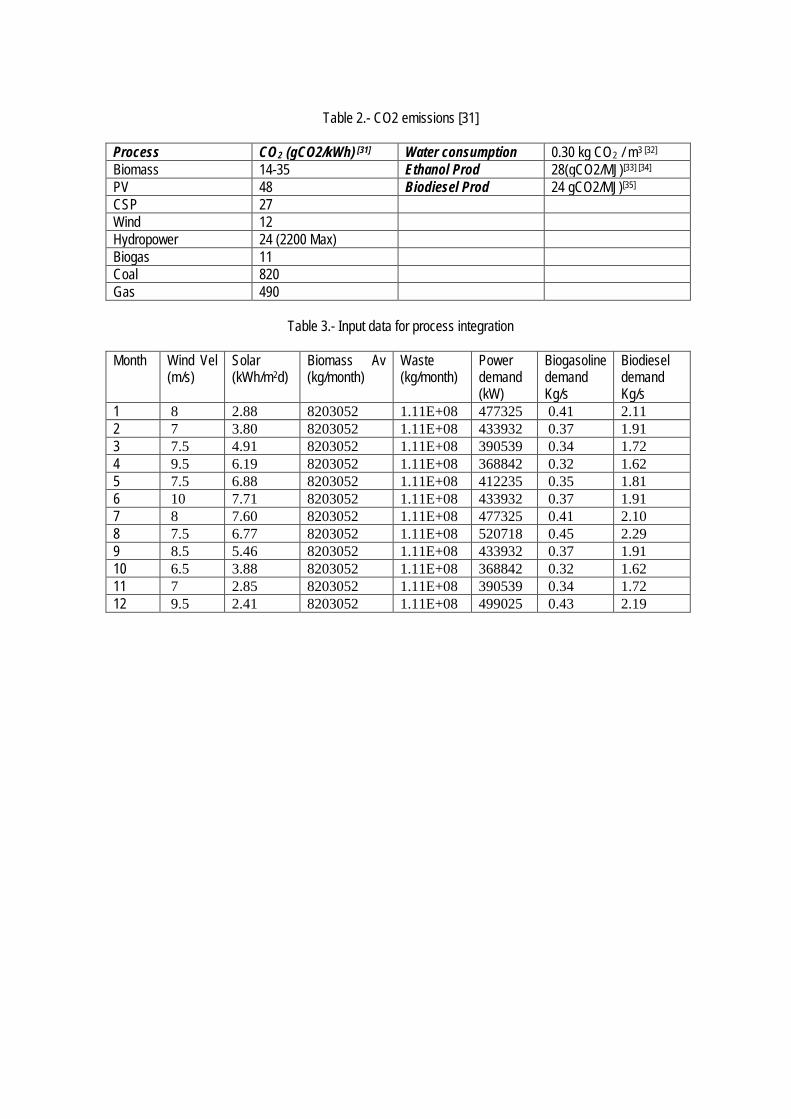
Table 2.- CO2 emissions [31]

Process CO2 (gCO2/kWh) Water consumption [31] 0.30 kg CO2 / m3 [32] Biomass 14-35 Ethanol Prod 28(gCO2/MJ)[33] [34]

PV 48 Biodiesel Prod 24 gCO2/MJ)[35] CSP 27 Wind 12 Hydropower 24 (2200 Max) Biogas 11 Coal 820 Gas 490

Table 3.- Input data for process integration

Month Wind Vel (m/s)

Solar (kWh/m2

Biomass Av (kg/month) d)

Waste (kg/month)

Power demand (kW)

Biogasoline demand Kg/s

Biodiesel demand Kg/s

1 8 2.88 8203052 1.11E+08 477325 0.41 2.11 2 7 3.80 8203052 1.11E+08 433932 0.37 1.91 3 7.5 4.91 8203052 1.11E+08 390539 0.34 1.72 4 9.5 6.19 8203052 1.11E+08 368842 0.32 1.62 5 7.5 6.88 8203052 1.11E+08 412235 0.35 1.81 6 10 7.71 8203052 1.11E+08 433932 0.37 1.91 7 8 7.60 8203052 1.11E+08 477325 0.41 2.10 8 7.5 6.77 8203052 1.11E+08 520718 0.45 2.29 9 8.5 5.46 8203052 1.11E+08 433932 0.37 1.91 10 6.5 3.88 8203052 1.11E+08 368842 0.32 1.62 11 7 2.85 8203052 1.11E+08 390539 0.34 1.72 12 9.5 2.41 8203052 1.11E+08 499025 0.43 2.19