optimal implicit strong stability preserving runge–kutta...
TRANSCRIPT

Optimal Implicit Strong Stability Preserving
Runge–Kutta Methods
David I. Ketcheson∗, Colin B. Macdonald†, Sigal Gottlieb‡.
February 21, 2008
Abstract
Strong stability preserving (SSP) time discretizations were devel-oped for use with spatial discretizations of partial differential equa-tions that are strongly stable under forward Euler time integration.SSP methods preserve convex boundedness and contractivity proper-ties satisfied by forward Euler, under a modified timestep restriction.We turn to implicit Runge–Kutta methods to alleviate this timesteprestriction, and present implicit SSP Runge–Kutta methods which areoptimal in the sense that they preserve convex boundedness propertiesunder the largest timestep possible among all methods with a givennumber of stages and order of accuracy. We consider methods up toorder six (the maximal order of SSP Runge–Kutta methods) and upto eleven stages. The numerically optimal methods found are all di-agonally implicit, leading us to conjecture that optimal implicit SSPRunge–Kutta methods are diagonally implicit. These methods allow alarger SSP timestep, compared to explicit methods of the same orderand number of stages. Numerical tests verify the order and the SSPproperty of the methods.
∗Department of Applied Mathematics, University of Washington, Seattle, WA 98195-2420 ([email protected]). The work of this author was funded by a U.S. Dept.of Energy Computational Science Graduate Fellowship.
†Department of Mathematics, Simon Fraser University, Burnaby, British Columbia,V5A1S6 Canada ([email protected]). The work of this author was partially supported by agrant from NSERC Canada and a scholarship from the Pacific Institute of Mathematics(PIMS).
‡Department of Mathematics, University of Massachusetts Dartmouth, North Dart-mouth MA 02747. This work was supported by AFOSR grant number FA9550-06-1-0255
1

Optimal SSP methods 2
1 Strong Stability Preserving Runge–Kutta
Methods
Strong stability preserving (SSP) Runge–Kutta methods are high-order timediscretization methods that preserve the strong stability properties—in anynorm or semi-norm—satisfied by a spatial discretization of a system of par-tial differential equations (PDEs) coupled with first-order forward Eulertimestepping [30, 28, 9, 10]. These methods were originally developed forthe numerical solution of hyperbolic PDEs to preserve the total variationdiminishing property satisfied by specially designed spatial discretizationscoupled with forward Euler integration.
In this work we are interested in approximating the solution of the ODE
ut = F (u), (1)
arising from the discretization of the spatial derivatives in the PDE
ut + f(u, ux, uxx, ...) = 0,
where the spatial discretization F (u) is chosen so that the solution obtainedusing the forward Euler method
un+1 = un + ∆tF (un), (2)
satisfies the monotonicity requirement
||un+1|| ≤ ||un||,
in some norm, semi-norm or convex functional || · ||, for a suitably restrictedtimestep
∆t ≤ ∆tFE.
If we write an explicit Runge–Kutta method in the now-standard Shu–Osher form [30]
u(0) = un,
u(i) =i−1∑
k=0
(
αi,ku(k) + ∆tβi,kF (u(k))
)
, αi,k ≥ 0, i = 1, . . . , s, (3)
un+1 = u(s),

Optimal SSP methods 3
then consistency requires that∑i−1
k=0 αi,k = 1. Thus, if αi,k ≥ 0 and βi,k ≥ 0,all the intermediate stages u(i) in (3) are simply convex combinations of
forward Euler steps, each with ∆t replaced byβi,k
αi,k∆t. Therefore, any bound
on a norm, semi-norm, or convex functional of the solution that is satisfiedby the forward Euler method will be preserved by the Runge–Kutta method,under the timestep restriction
βi,k
αi,k∆t ≤ ∆tFE, or equivalently
∆t ≤ minαi,kβi,k
∆tFE, (4)
where the minimum is taken over all k < i and βi,k 6= 0.These explicit SSP time discretizations can then be safely used with any
spatial discretization that satisfies the required stability property when cou-pled with forward Euler.
Definition 1. [Strong stability preserving (SSP)] For ∆tFE > 0, letF(∆tFE) denote the set of all pairs (F, ||·||) where the function F : R
m → Rm
and convex functional || · || are such that the numerical solution obtained bythe forward Euler method (2) satisfies ||un+1|| ≤ ||un|| whenever ∆t ≤ ∆tFE.Given a Runge–Kutta method, the SSP coefficient of the method is the largestconstant c ≥ 0 such that, for all (F, || · ||) ∈ F(∆tFE), the numerical solutiongiven by (3) satisfies ||u(i)|| ≤ ||un|| (for 1 ≤ i ≤ s) whenever
∆t ≤ c∆tFE. (5)
If c > 0, the method is said to be strong stability preserving under the max-imal timestep restriction (5).
A numerical method is said to be contractive if, for any two numericalsolutions u,v of (1) it holds that
||un+1 − vn+1|| ≤ ||un − vn||. (6)
Strong stability preserving methods are also of interest from the point ofview of preserving contractivity; in [4] it was shown that the SSP coefficientis equal to the radius of absolute monotonicity, which was shown in [22]to be the method-dependent factor in determining the largest timestep forcontractivity preservation.
If a particular spatial discretization coupled with the explicit forwardEuler method satisfies a strong stability property under some timestep re-striction, then the implicit backward Euler method satisfies the same strong

Optimal SSP methods 4
stability property, for any positive timestep [14]. However, all SSP Runge–Kutta methods of order greater than one suffer from some timestep restriction[10]. Much of the research in this field is devoted to finding methods thatare optimal in terms of their timestep restriction. For this purpose, variousimplicit extensions and generalizations of the Shu–Osher form have been in-troduced [10, 8, 6, 14]. The most general of these, and the form we use inthis paper, was introduced independently in [6] and [14]. We will refer to itas the modified Shu–Osher form.
The necessity of a finite timestep restriction for strong stability preserva-tion applies not only to Runge–Kutta methods, but also to linear multistepand all general linear methods [31]. Diagonally split Runge–Kutta methodslie outside this class and can be unconditionally contractive, but yield pooraccuracy for semi-discretizations of PDEs when used with large timesteps[25].
Optimal implicit SSP Runge–Kutta methods with up to two stages werefound in [16]. Recently, this topic was also studied by Ferracina & Spijker[7]; in that work, attention was restricted to the smaller class of singly di-agonally implicit Runge–Kutta (SDIRK) methods. They present optimalSDIRK methods of order p = 1 with any number of stages, order p = 2 withtwo stages, order p = 3 with two stages, and order p = 4 with three stages.They find numerically optimal methods of orders two to four and up to eightstages. Based on these results, they conjecture the form of optimal SDIRKmethods for second- and third-order and any number of stages.
In this work we consider the larger class of all Runge–Kutta methods,with up to eleven stages and sixth-order accuracy. Our search for new SSPmethods is facilitated by known results on contractivity and absolute mono-tonicity of Runge–Kutta methods [31, 22] and their connection to strongstability preservation [13, 14, 4, 6]. For a more detailed description of theShu–Osher form and the SSP property, we refer the interested reader to[30, 9, 10, 29, 8, 20].
The structure of this paper is as follows. In Section 2 we use results fromcontractivity theory to determine order barriers and other limitations on im-plicit SSP Runge–Kutta methods. In Section 3, we present new numericallyoptimal implicit Runge–Kutta methods of up to sixth order and up to elevenstages, found by numerical optimization. A few of these numerically optimalmethods are also proved to be truly optimal. We note that the numericallyoptimal implicit Runge–Kutta methods are all diagonally implicit, and thoseof order two and three are singly diagonally implicit. In Section 4 we present

Optimal SSP methods 5
numerical experiments using the numerically optimal implicit Runge–Kuttamethods, with a focus on verifying order of accuracy and the SSP timesteplimit. Finally, in Section 5 we summarize our results and discuss futuredirections.
2 Barriers and Limitations on SSP Methods
The theory of strong stability preserving Runge–Kutta methods is very closelyrelated to the concepts of absolute monotonicity and contractivity [13, 14, 4,6, 16]. In this section we review this connection and collect some results onabsolutely monotonic Runge–Kutta methods that allow us to draw conclu-sions about the class of implicit SSP Runge–Kutta methods. To facilitatethe discussion, we first review two representations of Runge–Kutta methods.
2.1 Representations of Runge–Kutta Methods
An s-stage Runge–Kutta method is usually represented by its Butcher tableau,consisting of an s× s matrix A and two s× 1 vectors b and c. The Runge–Kutta method defined by these arrays is
yi = un + ∆ts∑
j=1
aijF(
tn + cj∆t,yj)
, 1 ≤ i ≤ s, (7a)
un+1 = un + ∆t
s∑
j=1
bjF(
tn + cj∆t,yj)
. (7b)
It is convenient to define the (s+ 1) × s matrix
K =
(
AbT
)
,
and we will also make the standard assumption ci =∑s
j=1 aij . For the method(7) to be accurate to order p, the coefficients K must satisfy order conditions(see, e.g., [11]) denoted here by Φp(K) = 0.
A generalization of the Shu–Osher form (3) that applies to implicit aswell as explicit methods was introduced in [6, 14] to more easily study the
Optimal SSP methods 6
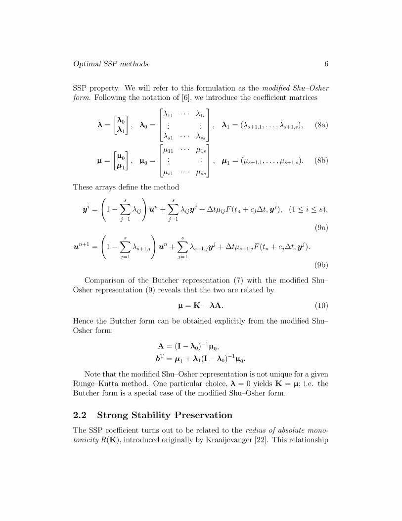
SSP property. We will refer to this formulation as the modified Shu–Osherform. Following the notation of [6], we introduce the coefficient matrices
λ =
[
λ0
λ1
]
, λ0 =
λ11 · · · λ1s...
...λs1 · · · λss
, λ1 = (λs+1,1, . . . , λs+1,s), (8a)
µ =
[
µ0
µ1
]
, µ0 =
µ11 · · · µ1s...
...µs1 · · · µss
, µ1 = (µs+1,1, . . . , µs+1,s). (8b)
These arrays define the method
yi =
(
1 −s∑
j=1
λij
)
un +
s∑
j=1
λijyj + ∆tµijF (tn + cj∆t,y
j), (1 ≤ i ≤ s),
(9a)
un+1 =
(
1 −s∑
j=1
λs+1,j
)
un +s∑
j=1
λs+1,jyj + ∆tµs+1,jF (tn + cj∆t,y
j).
(9b)
Comparison of the Butcher representation (7) with the modified Shu–Osher representation (9) reveals that the two are related by
µ = K − λA. (10)
Hence the Butcher form can be obtained explicitly from the modified Shu–Osher form:
A = (I − λ0)−1µ0,
bT = µ1 + λ1(I − λ0)−1µ0.
Note that the modified Shu–Osher representation is not unique for a givenRunge–Kutta method. One particular choice, λ = 0 yields K = µ; i.e. theButcher form is a special case of the modified Shu–Osher form.
2.2 Strong Stability Preservation
The SSP coefficient turns out to be related to the radius of absolute mono-tonicity R(K), introduced originally by Kraaijevanger [22]. This relationship

Optimal SSP methods 7
was proved in [4, 13], where also a more convenient, equivalent definition ofR(K) was given:
Definition 2. [Radius of absolute monotonicity (of a Runge–Kuttamethod)] The radius of absolute monotonicity R(K) of the Runge–Kuttamethod defined by Butcher array K is the largest value of r ≥ 0 such that(I + rA)−1 exists and
K(I + rA)−1 ≥ 0,
rK(I + rA)−1es ≤ es+1.
Here, the inequalities are understood component-wise and es denotes the s×1vector of ones.
From [6, Theorem 3.4], we obtain:
Theorem 1. Let an irreducible Runge–Kutta method be given by the Butcherarray K. Let c denote the SSP coefficient from Definition 1. Let R(K) denotethe radius of absolute monotonicity defined in Definition 2. Then
c = R(K).
Furthermore, there exists a modified Shu–Osher representation (λ,µ) suchthat (10) holds and
c = mini,j;i6=j
λi,jµi,j
,
where the minimum is taken over all µi,j 6= 0. In other words, the methodpreserves strong stability under the maximal timestep restriction
∆t ≤ R(K)∆tFE.
For a definition of reducibility see, e.g., [6, Definition 3.1]. If we replacethe assumption of irreducibility in the Theorem with the assumption c <∞, then the same results follow from [14, Propositions 2.1, 2.2 and 2.7].Furthermore, the restriction c < ∞ is not unduly restrictive in the presentwork because if c = ∞ then p = 1 [10], and we will be concerned only withmethods having p ≥ 2.
Although we are interested in strong stability preservation for general(nonlinear, nonautonomous) systems, it is useful for the purposes of this
Optimal SSP methods 8
section to introduce some concepts related to strong stability preservationfor linear autonomous systems.
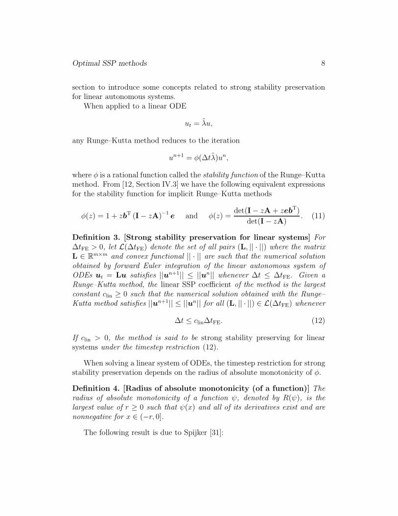
When applied to a linear ODE
ut = λ̃u,
any Runge–Kutta method reduces to the iteration
un+1 = φ(∆tλ̃)un,
where φ is a rational function called the stability function of the Runge–Kuttamethod. From [12, Section IV.3] we have the following equivalent expressionsfor the stability function for implicit Runge–Kutta methods
φ(z) = 1 + zbT (I − zA)−1e and φ(z) =
det(I − zA + zebT)
det(I − zA). (11)
Definition 3. [Strong stability preservation for linear systems] For∆tFE > 0, let L(∆tFE) denote the set of all pairs (L, || · ||) where the matrixL ∈ R
m×m and convex functional || · || are such that the numerical solutionobtained by forward Euler integration of the linear autonomous system ofODEs ut = Lu satisfies ||un+1|| ≤ ||un|| whenever ∆t ≤ ∆tFE. Given aRunge–Kutta method, the linear SSP coefficient of the method is the largestconstant clin ≥ 0 such that the numerical solution obtained with the Runge–Kutta method satisfies ||un+1|| ≤ ||un|| for all (L, || · ||) ∈ L(∆tFE) whenever
∆t ≤ clin∆tFE. (12)
If clin > 0, the method is said to be strong stability preserving for linearsystems under the timestep restriction (12).
When solving a linear system of ODEs, the timestep restriction for strongstability preservation depends on the radius of absolute monotonicity of φ.
Definition 4. [Radius of absolute monotonicity (of a function)] Theradius of absolute monotonicity of a function ψ, denoted by R(ψ), is thelargest value of r ≥ 0 such that ψ(x) and all of its derivatives exist and arenonnegative for x ∈ (−r, 0].
The following result is due to Spijker [31]:

Optimal SSP methods 9
Theorem 2. Let a Runge–Kutta method be given with stability function φ.Let clin denote the linear SSP coefficient of the method (see Definition 3).Then
clin = R(φ).
In other words, the method preserves strong stability for linear systems underthe maximal timestep restriction
∆t ≤ R(φ)∆tFE.
Because of this result, R(φ) is referred to as the threshold factor of themethod [31, 34]. Since L(h) ⊂ F(h), clearly c ≤ clin, so it follows that
R(K) ≤ R(φ). (13)
Optimal values of R(φ), for various classes of Runge–Kutta methods, canbe inferred from results found in [34], where the maximal value of R(ψ) wasstudied for ψ belonging to certain classes of rational functions.
In the following section, we use this equivalence between the radius ofabsolute monotonicity and the SSP coefficient to apply results regardingR(K) to the theory of SSP Runge–Kutta methods.
2.3 Order Barriers for SSP Runge–Kutta Methods
The SSP property is a very strong requirement, and imposes severe restric-tions on other properties of a Runge–Kutta method. We now review theseresults and draw a few additional conclusions that will guide our search foroptimal methods in the next section.
Some results in this and the next section will deal with the optimal valueof R(K) when K ranges over some class of methods. This optimal value willbe denoted by RIRK
s,p (resp., RERKs,p ) when K is permitted to be any implicit
(resp., explicit) Runge–Kutta method with at most s stages and at leastorder p.
The result below follows from [31, Theorem 1.3] and equation (13) above.
Result 1. Any Runge–Kutta method of order p > 1 has a finite radius ofabsolute monotonicity; i.e. RIRK
s,p <∞ for p > 1.
This is a disappointing result, which shows us that for SSP Runge–Kuttamethods of order greater than one we cannot avoid timestep restrictions
Optimal SSP methods 10
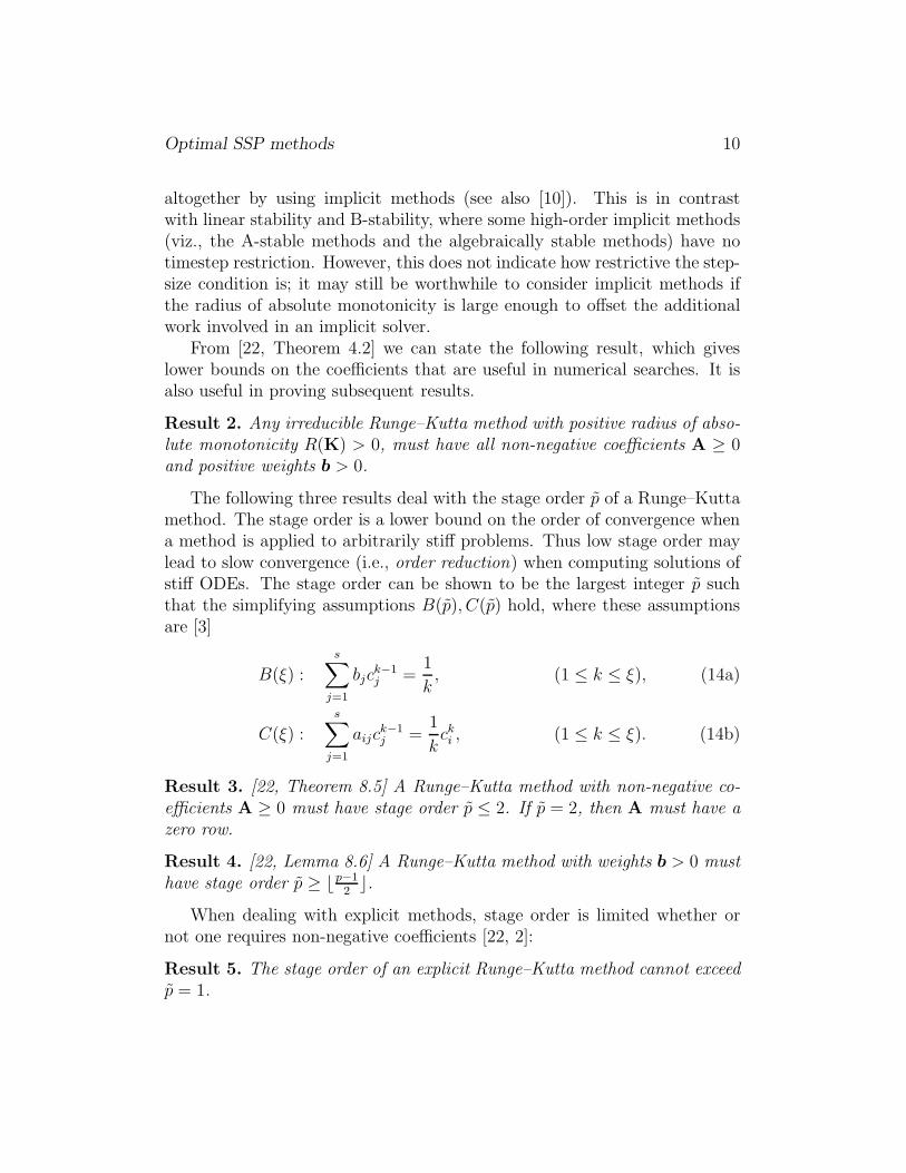
altogether by using implicit methods (see also [10]). This is in contrastwith linear stability and B-stability, where some high-order implicit methods(viz., the A-stable methods and the algebraically stable methods) have notimestep restriction. However, this does not indicate how restrictive the step-size condition is; it may still be worthwhile to consider implicit methods ifthe radius of absolute monotonicity is large enough to offset the additionalwork involved in an implicit solver.
From [22, Theorem 4.2] we can state the following result, which giveslower bounds on the coefficients that are useful in numerical searches. It isalso useful in proving subsequent results.
Result 2. Any irreducible Runge–Kutta method with positive radius of abso-lute monotonicity R(K) > 0, must have all non-negative coefficients A ≥ 0and positive weights b > 0.
The following three results deal with the stage order p̃ of a Runge–Kuttamethod. The stage order is a lower bound on the order of convergence whena method is applied to arbitrarily stiff problems. Thus low stage order maylead to slow convergence (i.e., order reduction) when computing solutions ofstiff ODEs. The stage order can be shown to be the largest integer p̃ suchthat the simplifying assumptions B(p̃), C(p̃) hold, where these assumptionsare [3]
B(ξ) :
s∑
j=1
bjck−1j =
1
k, (1 ≤ k ≤ ξ), (14a)
C(ξ) :s∑
j=1
aijck−1j =
1
kcki , (1 ≤ k ≤ ξ). (14b)
Result 3. [22, Theorem 8.5] A Runge–Kutta method with non-negative co-efficients A ≥ 0 must have stage order p̃ ≤ 2. If p̃ = 2, then A must have azero row.
Result 4. [22, Lemma 8.6] A Runge–Kutta method with weights b > 0 musthave stage order p̃ ≥ ⌊p−1
2⌋.
When dealing with explicit methods, stage order is limited whether ornot one requires non-negative coefficients [22, 2]:
Result 5. The stage order of an explicit Runge–Kutta method cannot exceedp̃ = 1.
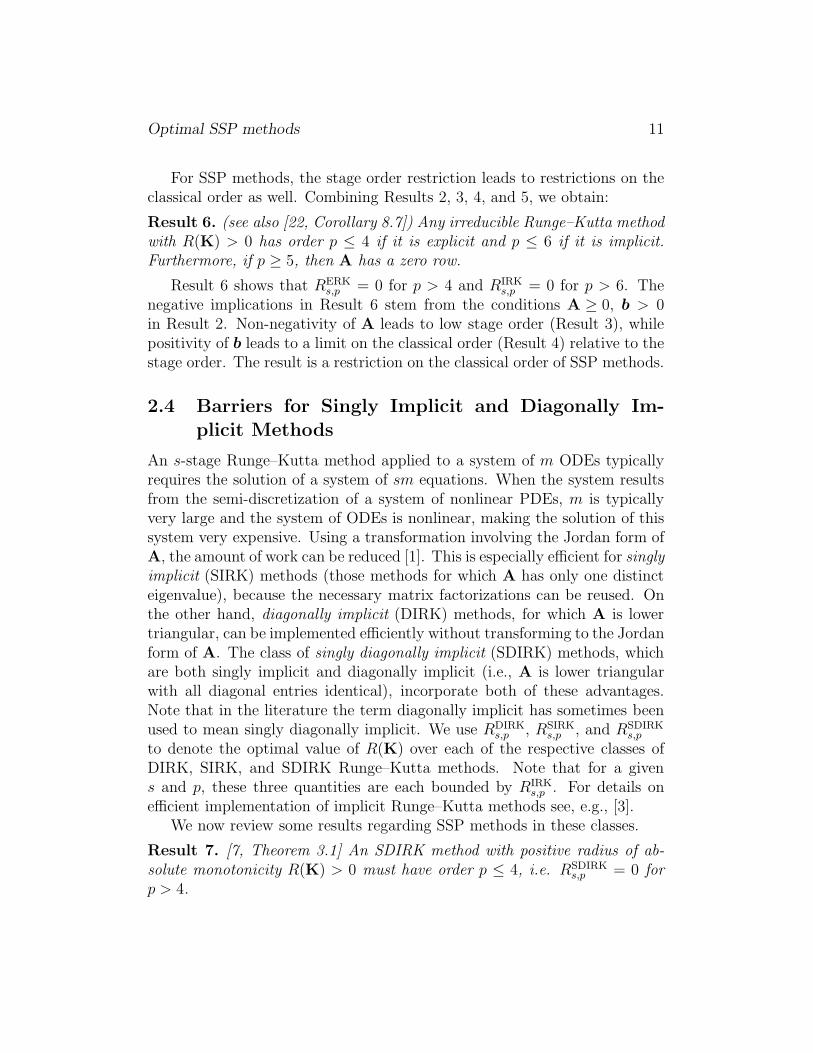
Optimal SSP methods 11
For SSP methods, the stage order restriction leads to restrictions on theclassical order as well. Combining Results 2, 3, 4, and 5, we obtain:
Result 6. (see also [22, Corollary 8.7]) Any irreducible Runge–Kutta methodwith R(K) > 0 has order p ≤ 4 if it is explicit and p ≤ 6 if it is implicit.Furthermore, if p ≥ 5, then A has a zero row.
Result 6 shows that RERKs,p = 0 for p > 4 and RIRK
s,p = 0 for p > 6. Thenegative implications in Result 6 stem from the conditions A ≥ 0, b > 0in Result 2. Non-negativity of A leads to low stage order (Result 3), whilepositivity of b leads to a limit on the classical order (Result 4) relative to thestage order. The result is a restriction on the classical order of SSP methods.
2.4 Barriers for Singly Implicit and Diagonally Im-plicit Methods
An s-stage Runge–Kutta method applied to a system of m ODEs typicallyrequires the solution of a system of sm equations. When the system resultsfrom the semi-discretization of a system of nonlinear PDEs, m is typicallyvery large and the system of ODEs is nonlinear, making the solution of thissystem very expensive. Using a transformation involving the Jordan form ofA, the amount of work can be reduced [1]. This is especially efficient for singlyimplicit (SIRK) methods (those methods for which A has only one distincteigenvalue), because the necessary matrix factorizations can be reused. Onthe other hand, diagonally implicit (DIRK) methods, for which A is lowertriangular, can be implemented efficiently without transforming to the Jordanform of A. The class of singly diagonally implicit (SDIRK) methods, whichare both singly implicit and diagonally implicit (i.e., A is lower triangularwith all diagonal entries identical), incorporate both of these advantages.Note that in the literature the term diagonally implicit has sometimes beenused to mean singly diagonally implicit. We use RDIRK
s,p , RSIRKs,p , and RSDIRK
s,p
to denote the optimal value of R(K) over each of the respective classes ofDIRK, SIRK, and SDIRK Runge–Kutta methods. Note that for a givens and p, these three quantities are each bounded by RIRK
s,p . For details onefficient implementation of implicit Runge–Kutta methods see, e.g., [3].
We now review some results regarding SSP methods in these classes.
Result 7. [7, Theorem 3.1] An SDIRK method with positive radius of ab-solute monotonicity R(K) > 0 must have order p ≤ 4, i.e. RSDIRK
s,p = 0 forp > 4.

Optimal SSP methods 12
Proposition 1. The order of an s-stage DIRK method when applied to alinear problem is at most s+ 1.
Proof. For a given s-stage DIRK method, let p denote its order and let φdenote its stability function. Then φ(x) = exp(x) + O(xp+1) as x → 0. Byequation (11), φ is a rational function whose numerator has degree at mosts. For DIRK methods, A is lower triangular, so by equation (11) the poles ofφ are the diagonal entries of A, which are real. A rational function with realpoles only and numerator of degree s approximates the exponential functionto order at most s+ 1 [3, Theorem 3.5.11]. Thus p ≤ s + 1.
Proposition 2. The order of an s-stage SIRK method with positive radiusof absolute monotonicity is at most s+ 1. Hence RSIRK
s,p = 0 for p > s+ 1.
Proof. For a given s-stage SIRK method, let p denote its order and let φdenote its stability function. Assume R(K) > 0; then by equation (13)R(φ) > 0. By equation (11), φ is a rational function whose numerator hasdegree at most s. For SIRK methods, equation (11) also implies that φ has aunique pole. Since R(φ) > 0, [34, Corollary 3.4] implies that this pole mustbe real. As in the proof above, [3, Theorem 3.5.11] then provides the desiredresult.
Result 6 implies that all eigenvalues of A must be zero, hence the stabilityfunction φ must be a polynomial. We thus have
Corollary 1. Consider the class of s-stage SIRK methods with order 5 ≤p ≤ 6 and R(K) > 0. Let Πn,p denote the set of all polynomials ψ of degreeless than or equal to n satisfying ψ(x) = exp(x) + O(xp+1) as x → 0. Thenfor 5 ≤ p ≤ 6,
RSIRKs,p ≤ sup
ψ∈Πs,p
R(ψ).
where the supremum over an empty set is taken to be zero. FurthermoreRSIRKs,p = 0 for 4 ≤ s < p ≤ 6.
The last statement of the Corollary follows from the observation that,since a polynomial approximates exp(x) to order at most equal to its degree,Πn,p is empty for p > s.
Corollary 1 implies that for s-stage SIRK methods of order p ≥ 5, R(K)is bounded by the optimal linear SSP coefficient of s-stage explicit Runge–Kutta methods of the same order (see [21, 17] for values of these optimalcoefficients).
Optimal SSP methods 13
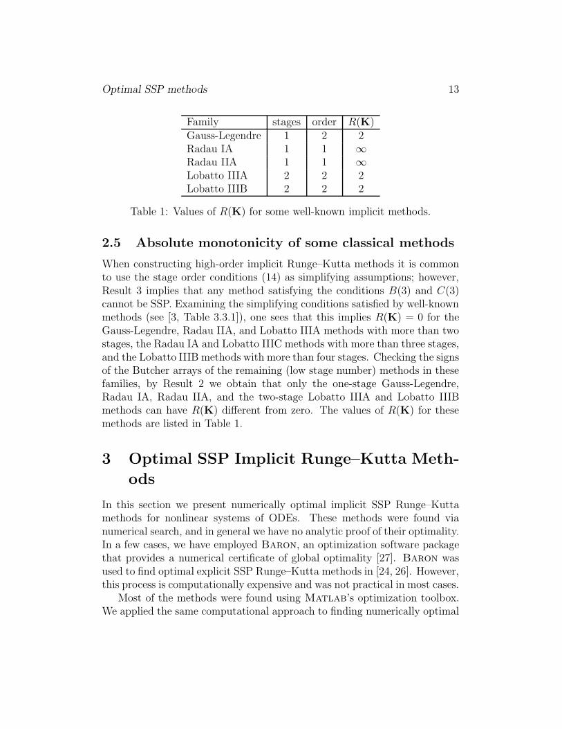
Family stages order R(K)Gauss-Legendre 1 2 2Radau IA 1 1 ∞Radau IIA 1 1 ∞Lobatto IIIA 2 2 2Lobatto IIIB 2 2 2
Table 1: Values of R(K) for some well-known implicit methods.
2.5 Absolute monotonicity of some classical methods
When constructing high-order implicit Runge–Kutta methods it is commonto use the stage order conditions (14) as simplifying assumptions; however,Result 3 implies that any method satisfying the conditions B(3) and C(3)cannot be SSP. Examining the simplifying conditions satisfied by well-knownmethods (see [3, Table 3.3.1]), one sees that this implies R(K) = 0 for theGauss-Legendre, Radau IIA, and Lobatto IIIA methods with more than twostages, the Radau IA and Lobatto IIIC methods with more than three stages,and the Lobatto IIIB methods with more than four stages. Checking the signsof the Butcher arrays of the remaining (low stage number) methods in thesefamilies, by Result 2 we obtain that only the one-stage Gauss-Legendre,Radau IA, Radau IIA, and the two-stage Lobatto IIIA and Lobatto IIIBmethods can have R(K) different from zero. The values of R(K) for thesemethods are listed in Table 1.
3 Optimal SSP Implicit Runge–Kutta Meth-
ods
In this section we present numerically optimal implicit SSP Runge–Kuttamethods for nonlinear systems of ODEs. These methods were found vianumerical search, and in general we have no analytic proof of their optimality.In a few cases, we have employed Baron, an optimization software packagethat provides a numerical certificate of global optimality [27]. Baron wasused to find optimal explicit SSP Runge–Kutta methods in [24, 26]. However,this process is computationally expensive and was not practical in most cases.
Most of the methods were found using Matlab’s optimization toolbox.We applied the same computational approach to finding numerically optimal

Optimal SSP methods 14
explicit and diagonally implicit SSP Runge–Kutta methods, and successfullyfound a solution at least as good as the previously best known solution inevery case. Because our approach was able to find these previously knownmethods, we expect that some of new methods—particularly those of lower-order or lower number of stages—may be globally optimal.
The optimization problem for general Runge–Kutta methods involves ap-proximately twice as many decision variables (dimensions) as the explicitor singly diagonally implicit cases, which have previously been investigated[9, 10, 32, 33, 26, 7]. Despite the larger number of decision variables, wehave been able to find numerically optimal methods even for large numbersof stages. We attribute this success to the reformulation of the optimizationproblem in terms of the Butcher coefficients rather than the Shu–Osher co-efficients, as suggested in [5]. Specifically, we solve the optimization problem
maxK
r, (15a)
subject to
K(I + rA)−1 ≥ 0,
rK(I + rA)−1es ≤ es+1,
Φp(K) = 0,
(15b)
where the inequalities are understood component-wise and recall that Φp(K)represents the order conditions up to order p. This formulation, implementedin Matlab using a sequential quadratic programming approach (fmincon inthe optimization toolbox), was used to find the methods given below. Ina concurrent effort, this formulation has been used to search for optimalexplicit SSP methods [17].
Because in most cases we cannot prove the optimality of the resultingmethods, we use hats to denote the best value found by numerical search,e.g. R̂IRK
s,p , etc.The above problem can be reformulated (using a standard approach for
converting rational constraints to polynomial constraints) as
maxK,µ
r, (16a)
subject to
µ ≥ 0,
rµes ≤ es+1,
K = µ(I + rA),
Φp(K) = 0.
(16b)

Optimal SSP methods 15
This optimization problem has only polynomial constraints and thus is appro-priate for the Baron optimization software which requires such constraintsto be able to guarantee global optimality [27]. Note that µ in (16) corre-sponds to one possible modified Shu–Osher form with λ = rµ.
In comparing methods with different numbers of stages, one is usuallyinterested in the relative time advancement per computational cost. Fordiagonally implicit methods, the computational cost per time-step is pro-portional to the number of stages. We therefore define the effective SSPcoefficient of a method as R(K)
s; this normalization enables us to compare the
cost of integration up to a given time using DIRK schemes of order p > 1.However, for non-DIRK methods of various s, it is much less obvious how tocompare computation cost.
In the following, we give modified Shu–Osher arrays for the numericallyoptimal methods. To simplify implementation, we present modified Shu–Osher arrays in which the diagonal elements of λ are zero. This form is asimple rearrangement and involves no loss of generality.
3.1 Second-order Methods
Optimizing over the class of all (s ≤ 11)-stage second-order implicit Runge–Kutta methods we found that the numerically optimal methods are, remark-ably, identical to the numerically optimal SDIRK methods found in [5, 7].This result stresses the importance of the second-order SDIRK methodsfound in [5, 7]: they appear to be optimal not only among SDIRK meth-ods, but also among the larger class of all implicit Runge–Kutta methods.
These methods are most advantageously implemented in a certain mod-ified Shu–Osher form. This is because these arrays (if chosen carefully) aremore sparse. In fact, for these methods there exist modified Shu–Osher ar-rays that are bidiagonal. We give the general formulae here.
The numerically optimal second-order method with s stages has R(K) =2s and coefficients
λ =
01 0
1. . .. . . 0
1
, µ =
12s12s
12s
12s
. . .
. . . 12s12s
. (17)

Optimal SSP methods 16
The one-stage method of this class is the implicit midpoint rule, whilethe s-stage method is equivalent to s successive applications of the implicitmidpoint rule (as was observed in [5]). Thus these methods inherit the de-sirable properties of the implicit midpoint rule such as algebraic stabilityand A-stability [12]. Of course, since they all have the same effective SSPcoefficient R(K)/s = 2, they are all essentially equivalent.
The one-stage method is the unique method with s = 1, p = 2 and henceis optimal. The two-stage method achieves the maximum radius of absolutemonotonicity for rational functions that approximate the exponential to sec-ond order with numerator and denominator of degree at most two, hence itis optimal to within numerical precision [34, 16, 7]. In addition to duplicat-ing these optimality results, Baron was used to numerically prove that thes = 3 scheme is globally optimal, verifying [7, Conjecture 3.1] for the cases = 3. The s = 1 and s = 2 cases required only several seconds but the s = 3case took much longer, requiring approximately 11 hours of CPU time on anAthlon MP 2800+ processor.
While the remaining methods have not been proven optimal, it appearslikely that they may be. From multiple random initial guesses, the optimiza-tion algorithm consistently converges to the same method, or to a reduciblemethod corresponding to one of the numerically optimal methods with asmaller number of stages. Also, many of the inequality constraints are satis-fied exactly for these methods. Furthermore, the methods all have a similarform, depending only on the stage number. These observations suggest:
Conjecture 1. (An extension of [7, Conjecture 3.1]) The optimal second-order s-stage implicit SSP method is given by the SDIRK method (17) andhence RIRK
s,2 = 2s.
This conjecture would imply that the effective SSP coefficient of anyRunge–Kutta method of order greater than one is at most equal to two.
3.2 Third-order Methods
The numerically optimal third-order implicit Runge–Kutta methods withs ≥ 2 stages are also SDIRK and identical to the numerically optimal SDIRKmethods found in [5, 7], which have R(K) = s − 1 +
√s2 − 1. Once again,
these results indicate that the methods found in [5, 7] are likely optimal overthe entire class of implicit Runge–Kutta methods.

Optimal SSP methods 17
In this case, too, when implementing these methods it is possible to usebidiagonal Shu–Osher arrays. For p = 3 and s ≥ 2 the numerically optimalmethods have coefficients
µ =
µ11
µ21. . .. . . µ11
µ21 µ11
µs+1,s
, λ =
0
1. . .. . . 0
1 0λs+1,s
, (18a)
where
µ11 =1
2
(
1 −√
s− 1
s+ 1
)
, µ21 =1
2
(
√
s+ 1
s− 1− 1
)
, (18b)
µs+1,s =s+ 1
s(s+ 1 +√s2 − 1)
, λs+1,s =(s+ 1)(s− 1 +
√s2 − 1)
s(s+ 1 +√s2 − 1)
. (18c)
The two-stage method in this family achieves the maximum value of R(φ)found in [34] for φ in the set of third-order rational approximations to theexponential with numerator and denominator of degree at most 2. Since thecorresponding one-parameter optimization problem is easy to solve, then (inview of (13)) the method is clearly optimal to within numerical precision.Baron was used to numerically prove global optimality for the three-stagemethod (18), requiring about 12 hours of CPU time on an Athlon MP 2800+processor. Note that this verifies [7, Conjecture 3.2] for the case s = 3.
While the remaining methods (those with s ≥ 4) have not been provenoptimal, we are again led to suspect that they may be, because of the natureof the optimal methods and the convergent behavior of the optimizationalgorithm for these cases. These observations suggest:
Conjecture 2. (An extension of [7, Conjecture 3.2]) For s ≥ 2, the optimalthird-order s-stage implicit Runge–Kutta SSP method is given by the SDIRKmethod (18) and hence RIRK
s,3 = s− 1 +√s2 − 1.
3.3 Fourth-order Methods
Based on the above results, one might suspect that all optimal implicit SSPmethods are singly diagonally implicit. In fact, this cannot hold for p ≥ 5

Optimal SSP methods 18
since in that case A must have a zero row (see Result 6 above). The nu-merically optimal methods of fourth-order are not singly diagonally impliciteither; however, all numerically optimal fourth-order methods we have foundare diagonally implicit.
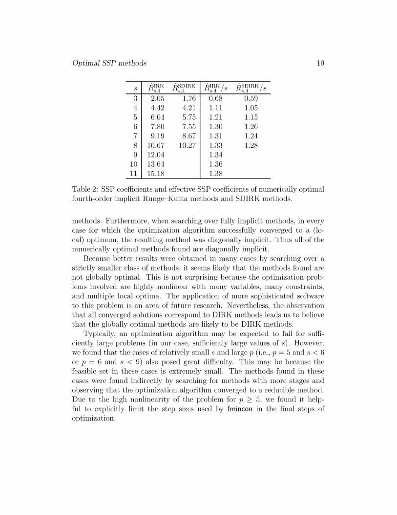
The unique two-stage fourth-order Runge–Kutta method has a negativecoefficient and so is not SSP. Thus we begin our search with three-stagemethods. We list the SSP coefficients and effective SSP coefficients of thenumerically optimal methods in Table 2. For comparison, the table also liststhe effective SSP coefficients of the numerically optimal SDIRK methodsfound in [7]. Our numerically optimal DIRK methods have larger SSP coef-ficients in every case. Furthermore, they have representations that allow forvery efficient implementation in terms of storage. However, SDIRK methodsmay be implemented in a potentially more efficient (in terms of computation)manner than DIRK methods. An exact evaluation of the relative efficienciesof these methods is beyond the scope of this work. The coefficients of the4-stage method are included in Table 7. The coefficients of the remainingmethods are available from [19, 18].
Baron was run on the three-stage fourth-order case but was unable toprove the global optimality of the resulting method using 14 days of CPUtime on an Athlon MP 2800+ processor. However, during that time Baron
did establish an upper bound RIRK3,4 ≤ 3.234. Baron was not run on any
other fourth-order cases, nor was it used for p = 5 or p = 6.Although none of the fourth-order methods are proven optimal, it appears
that they may be optimal. This is again because the optimization algorithmis able to converge to these methods from a range of random initial guesses,and because very many of the inequality constraints are satisfied exactlyfor these methods. Additionally, we were able to recover all of the optimalfourth-order SDIRK methods of [7] by restricting our search to the space ofSDIRK methods.
3.4 Fifth- and Sixth-order Methods
We have found fifth- and sixth-order SSP methods with up to eleven stages.Two sets of numerical searches were conducted, corresponding to optimiza-tion over the full class of implicit Runge–Kutta methods and optimizationover the subclass of diagonally implicit Runge–Kutta methods. More CPUtime was devoted to the first set of searches; however, in most cases the bestmethods we were able to find resulted from the searches restricted to DIRK
Optimal SSP methods 19
s R̂IRKs,4 R̂SDIRK
s,4 R̂IRKs,4 /s R̂SDIRK
s,4 /s
3 2.05 1.76 0.68 0.594 4.42 4.21 1.11 1.055 6.04 5.75 1.21 1.156 7.80 7.55 1.30 1.267 9.19 8.67 1.31 1.248 10.67 10.27 1.33 1.289 12.04 1.34
10 13.64 1.3611 15.18 1.38
Table 2: SSP coefficients and effective SSP coefficients of numerically optimalfourth-order implicit Runge–Kutta methods and SDIRK methods.
methods. Furthermore, when searching over fully implicit methods, in everycase for which the optimization algorithm successfully converged to a (lo-cal) optimum, the resulting method was diagonally implicit. Thus all of thenumerically optimal methods found are diagonally implicit.
Because better results were obtained in many cases by searching over astrictly smaller class of methods, it seems likely that the methods found arenot globally optimal. This is not surprising because the optimization prob-lems involved are highly nonlinear with many variables, many constraints,and multiple local optima. The application of more sophisticated softwareto this problem is an area of future research. Nevertheless, the observationthat all converged solutions correspond to DIRK methods leads us to believethat the globally optimal methods are likely to be DIRK methods.
Typically, an optimization algorithm may be expected to fail for suffi-ciently large problems (in our case, sufficiently large values of s). However,we found that the cases of relatively small s and large p (i.e., p = 5 and s < 6or p = 6 and s < 9) also posed great difficulty. This may be because thefeasible set in these cases is extremely small. The methods found in thesecases were found indirectly by searching for methods with more stages andobserving that the optimization algorithm converged to a reducible method.Due to the high nonlinearity of the problem for p ≥ 5, we found it help-ful to explicitly limit the step sizes used by fmincon in the final steps ofoptimization.

Optimal SSP methods 20
s R̂IRKs,5 RSIRK
s,5 R̂IRKs,5 /s RSIRK
s,5 /s(upper bound) (upper bound)
4 1.14 0.295 3.19 1.00 0.64 0.206 4.97 2.00 0.83 0.337 6.21 2.65 0.89 0.388 7.56 3.37 0.94 0.429 8.90 4.10 0.99 0.4610 10.13 4.83 1.01 0.4811 11.33 5.52 1.03 0.50
Table 3: Comparison of SSP coefficients of numerically optimal fifth-orderIRK methods with theoretical upper bounds on SSP coefficients of fifth-orderSIRK methods.
3.4.1 Fifth-order Methods
Three stages Using the W transformation [3] we find the one parameterfamily of three-stage, fifth-order methods
A =
536
+ 29γ 5
36+ 1
24
√15 − 5
18γ 5
36+ 1
30
√15 + 2
9γ
29− 1
15
√15 − 4
9γ 2
9+ 5
9γ 2
9+ 1
15
√15 − 4
9γ
536
− 130
√15 + 2
9γ 5
36− 1
24
√15 − 5
18γ 5
36+ 2
9γ
.
It is impossible to choose γ so that a21 and a31 are simultaneously nonnega-tive, so there are no SSP methods in this class.
Four to Eleven stages We list the time-step coefficients and effectiveSSP coefficients of the numerically optimal fifth order implicit Runge–Kuttamethods for 4 ≤ s ≤ 11 in Table 3. It turns out that all of these methodsare diagonally implicit.
For comparison, we also list the upper bounds on effective SSP coefficientsof SIRK methods in these classes implied by combining Corollary 1 with [17,Table 2.1]. Our numerically optimal IRK methods have larger effective SSPcoefficients in every case. The coefficients of the optimal five-stage methodare listed in Table 8. Coefficients of the remaining methods are availablefrom [19, 18].
Optimal SSP methods 21
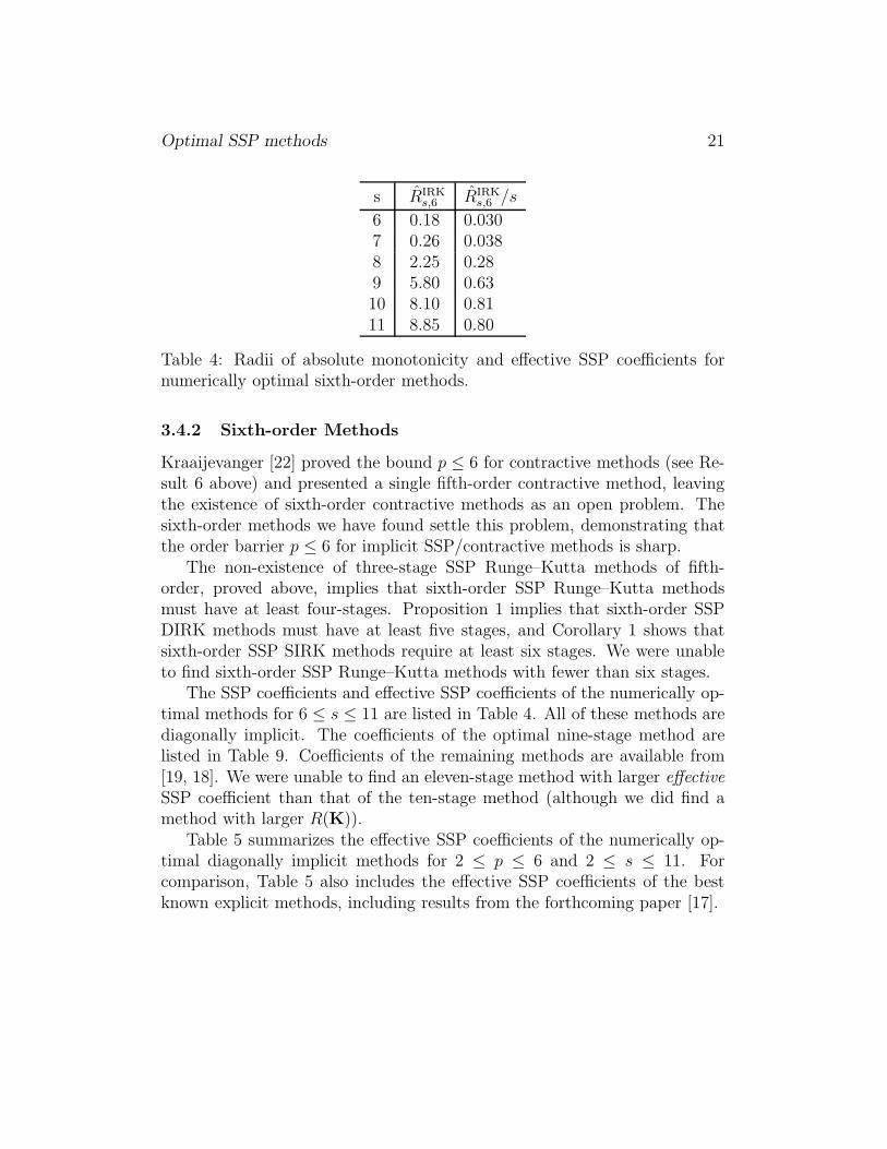
s R̂IRKs,6 R̂IRK
s,6 /s
6 0.18 0.0307 0.26 0.0388 2.25 0.289 5.80 0.6310 8.10 0.8111 8.85 0.80
Table 4: Radii of absolute monotonicity and effective SSP coefficients fornumerically optimal sixth-order methods.
3.4.2 Sixth-order Methods
Kraaijevanger [22] proved the bound p ≤ 6 for contractive methods (see Re-sult 6 above) and presented a single fifth-order contractive method, leavingthe existence of sixth-order contractive methods as an open problem. Thesixth-order methods we have found settle this problem, demonstrating thatthe order barrier p ≤ 6 for implicit SSP/contractive methods is sharp.
The non-existence of three-stage SSP Runge–Kutta methods of fifth-order, proved above, implies that sixth-order SSP Runge–Kutta methodsmust have at least four-stages. Proposition 1 implies that sixth-order SSPDIRK methods must have at least five stages, and Corollary 1 shows thatsixth-order SSP SIRK methods require at least six stages. We were unableto find sixth-order SSP Runge–Kutta methods with fewer than six stages.
The SSP coefficients and effective SSP coefficients of the numerically op-timal methods for 6 ≤ s ≤ 11 are listed in Table 4. All of these methods arediagonally implicit. The coefficients of the optimal nine-stage method arelisted in Table 9. Coefficients of the remaining methods are available from[19, 18]. We were unable to find an eleven-stage method with larger effectiveSSP coefficient than that of the ten-stage method (although we did find amethod with larger R(K)).
Table 5 summarizes the effective SSP coefficients of the numerically op-timal diagonally implicit methods for 2 ≤ p ≤ 6 and 2 ≤ s ≤ 11. Forcomparison, Table 5 also includes the effective SSP coefficients of the bestknown explicit methods, including results from the forthcoming paper [17].
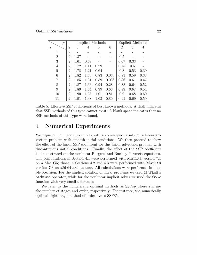
Optimal SSP methods 22
HH
HH
HH
sp Implicit Methods Explicit Methods
2 3 4 5 6 2 3 41 2 - - - - - - -2 2 1.37 - - - 0.5 - -3 2 1.61 0.68 - - 0.67 0.33 -4 2 1.72 1.11 0.29 0.75 0.5 -5 2 1.78 1.21 0.64 0.8 0.53 0.306 2 1.82 1.30 0.83 0.030 0.83 0.59 0.387 2 1.85 1.31 0.89 0.038 0.86 0.61 0.478 2 1.87 1.33 0.94 0.28 0.88 0.64 0.529 2 1.89 1.34 0.99 0.63 0.89 0.67 0.5410 2 1.90 1.36 1.01 0.81 0.9 0.68 0.6011 2 1.91 1.38 1.03 0.80 0.91 0.69 0.59
Table 5: Effective SSP coefficients of best known methods. A dash indicatesthat SSP methods of this type cannot exist. A blank space indicates that noSSP methods of this type were found.
4 Numerical Experiments
We begin our numerical examples with a convergence study on a linear ad-vection problem with smooth initial conditions. We then proceed to showthe effect of the linear SSP coefficient for this linear advection problem withdiscontinuous initial conditions. Finally, the effect of the SSP coefficientis demonstrated on the nonlinear Burgers’ and Buckley–Leverett equations.The computations in Section 4.1 were performed with Matlab version 7.1on a Mac G5; those in Sections 4.2 and 4.3 were performed with Matlab
version 7.3 on x86-64 architecture. All calculations were performed in dou-ble precision. For the implicit solution of linear problems we used Matlab’sbackslash operator, while for the nonlinear implicit solves we used the fsolve
function with very small tolerances.We refer to the numerically optimal methods as SSPsp where s, p are
the number of stages and order, respectively. For instance, the numericallyoptimal eight-stage method of order five is SSP85.

Optimal SSP methods 23
4.1 Linear Advection
The prototypical hyperbolic PDE is the linear wave equation,
ut + aux = 0, 0 ≤ x ≤ 2π. (19)
We consider (19) with a = −2π, periodic boundary conditions and vari-ous initial conditions. We use a method-of-lines approach, discretizing theinterval (0, 2π] into m points xj = j∆x, j = 1, . . . , m, and then discretiz-ing −aux with first-order upwind finite differences. We solve the resultingsystem (1) using our timestepping schemes. To isolate the effect of the time-discretization error, we exclude the effect of the error associated with thespatial discretization by comparing the numerical solution to the exact solu-tion of the ODE system, rather than to the exact solution of the PDE (19). Inlieu of the exact solution we use a very accurate numerical solution obtainedusing Matlab’s ode45 solver with minimal tolerances (AbsTol = 1 × 10⁻¹⁴,RelTol = 1 × 10⁻¹³).
Figure 1 shows a convergence study for various numerically optimal schemesfor the problem (19) with m = 120 points in space and smooth initial data
u(0, x) = sin(x),
advected until final time tf = 1. Here σ indicates the size of the timestep:∆t = σ∆tFE. The results show that all the methods achieve their designorder.
Now consider the advection equation with discontinuous initial data
u(x, 0) =
{
1 if π2≤ x ≤ 3π
2,
0 otherwise.(20)
Figure 2 shows a convergence study for the third-order methods with s = 3to s = 8 stages, for tf = 1 using m = 64 points and the first-order upwindingspatial discretization. Again, the results show that all the methods achievetheir design order. Finally, we note that the higher-stage methods give asmaller error for the same timestep; that is as s increases, the error constantof the method decreases.
Figure 3 shows the result of solving the discontinuous advection exampleusing the two-stage third-order method over a single timestep with m = 200.For this linear autonomous system, the theoretical monotonicity-preservingtimestep bound is σ ≤ clin = 2.732. We see that as the timestep is increased,the line steepens and forms a small step, which becomes an oscillation as thestability limit is exceeded, and worsens as the timestep is raised further.

Optimal SSP methods 24
100
101
10−6
10−4
10−2
100
σ
L ∞ e
rror
Advection of a Sine Wave
p = 3
SSP33SSP43SSP53SSP63SSP73SSP83
100
10110
−15
10−10
10−5
σL ∞
err
or
Advection of a Sine Wave
p = 4
p = 5
p = 6
SSP54SSP64SSP85SSP116
Figure 1: Convergence of various numerically optimal SSP methods for linearadvection of a sine wave.
100
10110
−6
10−4
10−2
σ
L ∞ e
rror
Advection of a Square Wave
p = 3
SSP33SSP43SSP53SSP63SSP73SSP83
Figure 2: Convergence of third-order methods for linear advection of a squarewave.

Optimal SSP methods 25
0 0.5 1 1.5 2 2.5 3
0
0.2
0.4
0.6
0.8
1
x
u
(a) σ = 2.0
0 0.5 1 1.5 2 2.5 3
0
0.2
0.4
0.6
0.8
1
x
u
(b) σ = 2.5
0 0.5 1 1.5 2 2.5 3
0
0.2
0.4
0.6
0.8
1
x
u
(c) σ = 2.7
0 0.5 1 1.5 2 2.5 3
0
0.2
0.4
0.6
0.8
1
x
u
(d) σ = 2.8
0 0.5 1 1.5 2 2.5 3
0
0.2
0.4
0.6
0.8
1
x
u
(e) σ = 3.0
0 0.5 1 1.5 2 2.5 3
0
0.2
0.4
0.6
0.8
1
x
u
(f) σ = 3.6
Figure 3: Solution of the linear advection problem after one timestep withthe two-stage third-order method (clin = 2.732).
Optimal SSP methods 26
0 0.5 1 1.5 20.2
0.3
0.4
0.5
0.6
0.7
0.8
0.9
x
u
ref. soln.SSP53
(a) σ = 8
0 0.5 1 1.5 20.2
0.3
0.4
0.5
0.6
0.7
0.8
0.9
x
u
ref. soln.SSP53
(b) σ = 32
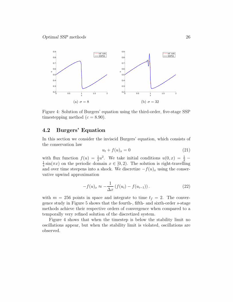
Figure 4: Solution of Burgers’ equation using the third-order, five-stage SSPtimestepping method (c = 8.90).
4.2 Burgers’ Equation
In this section we consider the inviscid Burgers’ equation, which consists ofthe conservation law
ut + f(u)x = 0 (21)
with flux function f(u) = 12u2. We take initial conditions u(0, x) = 1
2−
14sin(πx) on the periodic domain x ∈ [0, 2). The solution is right-travelling
and over time steepens into a shock. We discretize −f(u)x using the conser-vative upwind approximation
−f(u)x ≈ − 1
∆x(f(ui) − f(ui−1)) . (22)
with m = 256 points in space and integrate to time tf = 2. The conver-gence study in Figure 5 shows that the fourth-, fifth- and sixth-order s-stagemethods achieve their respective orders of convergence when compared to atemporally very refined solution of the discretized system.
Figure 4 shows that when the timestep is below the stability limit nooscillations appear, but when the stability limit is violated, oscillations areobserved.

Optimal SSP methods 27
100
101
10−10
10−5
p = 4
σ
L ∞ e
rror
Burgers’ Equation
SSP34SSP44SSP54SSP64SSP74SSP84SSP94SSP10,4SSP11,4
100
101
10−10
10−5
p = 5
σ
L ∞ e
rror
Burgers’ Equation
SSP45SSP55SSP65SSP75SSP85SSP95SSP10,5SSP11,5
100
101
10−10
10−5
p = 6
σ
L ∞ e
rror
Burgers’ Equation
SSP66SSP76SSP86SSP96SSP10,6
Figure 5: Convergence of the numerically optimal fourth-, fifth- and sixth-order schemes on Burgers’ equation. The solid circles indicate σ = c for eachscheme.
Optimal SSP methods 28
4.3 Buckley–Leverett Equation
The Buckley–Leverett equation is a model for two-phase flow through porousmedia [23] and consists of the conservation law (21) with flux function
f(u) =u2
u2 + a(1 − u)2.
We take a = 13
and initial conditions
u(x, 0) =
{
1 if x ≤ 12,
0 otherwise,
on x ∈ [0, 1) with periodic boundary conditions. Our spatial discretizationuses m = 100 points and we use the conservative scheme with Koren limiterused in [7] and [15, Section III.1]. The nonlinear system of equations for eachstage of the Runge–Kutta method is solved with Matlab’s fsolve, with theJacobian approximated [15] by that of the first-order upwind discretization(22). We compute the solution for n =
⌈
18
1∆t
⌉
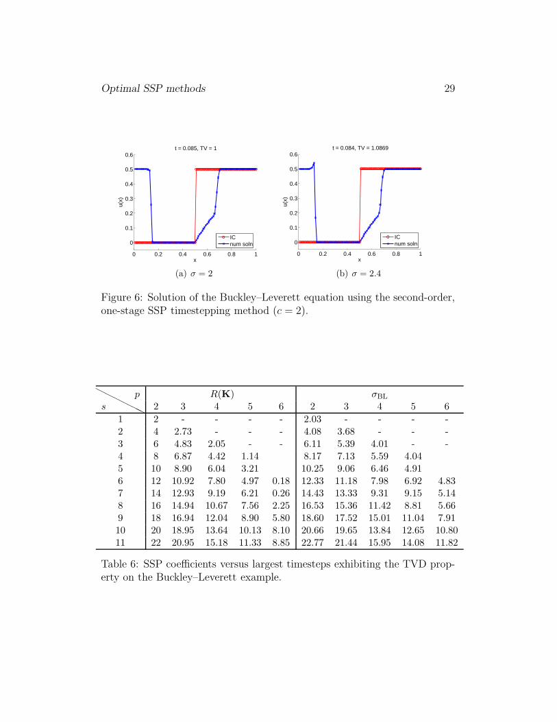
timesteps.For this problem, as in [7], we find that the forward Euler solution is
total variation diminishing (TVD) for ∆t ≤ ∆tFE = 0.0025. Figure 6 showstypical solutions for the SSP(1,2) scheme with timestep ∆t = σ∆tFE. Table 6compares the SSP coefficient R(K) with σBL = ∆tRK/∆tFE, where ∆tRK isthe largest observed timestep for which the numerical solution obtained withthe Runge–Kutta method is TVD. We note that, for each method, the valueof σBL is greater than the SSP coefficient. In fact, at least for either lowerorder p or high number of stages s, the values are in good correspondence.For p = 2 and p = 3, our results agree with those of [7].
5 Conclusions and Future Work
By numerical optimization we have found implicit strong stability preservingRunge–Kutta methods of order up to the maximum possible of p = 6 andstages up to s = 11. Methods with up to three stages and third order ofaccuracy have been proven optimal by analysis or by the global optimizationsoftware package Baron. Remarkably, the numerically optimal methods ofup to third-order are singly diagonally implicit, and the numerically optimalmethods of all orders are diagonally implicit. Furthermore, all of the local op-tima found in our searches correspond to diagonally implicit methods. Based
Optimal SSP methods 29
0 0.2 0.4 0.6 0.8 1
0
0.1
0.2
0.3
0.4
0.5
0.6
x
u(x)
t = 0.085, TV = 1
ICnum soln
(a) σ = 2
0 0.2 0.4 0.6 0.8 1
0
0.1
0.2
0.3
0.4
0.5
0.6
x
u(x)
t = 0.084, TV = 1.0869
ICnum soln
(b) σ = 2.4
Figure 6: Solution of the Buckley–Leverett equation using the second-order,one-stage SSP timestepping method (c = 2).
HH
HH
HHs
p R(K) σBL
2 3 4 5 6 2 3 4 5 6
1 2 - - - - 2.03 - - - -2 4 2.73 - - - 4.08 3.68 - - -3 6 4.83 2.05 - - 6.11 5.39 4.01 - -4 8 6.87 4.42 1.14 8.17 7.13 5.59 4.045 10 8.90 6.04 3.21 10.25 9.06 6.46 4.916 12 10.92 7.80 4.97 0.18 12.33 11.18 7.98 6.92 4.837 14 12.93 9.19 6.21 0.26 14.43 13.33 9.31 9.15 5.148 16 14.94 10.67 7.56 2.25 16.53 15.36 11.42 8.81 5.669 18 16.94 12.04 8.90 5.80 18.60 17.52 15.01 11.04 7.9110 20 18.95 13.64 10.13 8.10 20.66 19.65 13.84 12.65 10.8011 22 20.95 15.18 11.33 8.85 22.77 21.44 15.95 14.08 11.82
Table 6: SSP coefficients versus largest timesteps exhibiting the TVD prop-erty on the Buckley–Leverett example.
Optimal SSP methods 30
on these results, we conjecture that the optimal implicit SSP Runge–Kuttamethods of any number of stages are diagonally implicit. Future work mayinvolve numerical experiments with more powerful numerical optimizationsoftware, which will allow us to search more thoroughly and among methodswith more stages to support this conjecture.
The likelihood that our numerically optimal methods are nearly or trulyoptimal can be inferred to some extent from the behavior of Matlab’s opti-mization toolbox. For the methods of up to fourth-order, the software is ableto repeatedly converge to the optimal solution from a wide range of initialguesses. Hence we expect that these methods are optimal, or very nearly so.For methods of fifth- and sixth-order, the behavior of Matlab’s toolbox ismore erratic and it is difficult to determine how close to optimal the methodsare. By comparing them with methods of the same number of stages andlower order, however, we see that in most cases the SSP coefficients of theglobally optimal methods cannot be dramatically larger than those we havefound.
Numerical experiments confirm the theoretical properties of these meth-ods. The implicit SSP Runge–Kutta methods we found have SSP coefficientssignificantly larger than those of optimal explicit methods for a given num-ber of stages and order of accuracy. Furthermore, we have provided implicitmethods of orders five and six, whereas explicit methods can have order atmost four. However, these advantages in accuracy and timestep restrictionmust be weighed against the cost of solving the implicit set of equations.In the future we plan to compare in practice the relative efficiency of thesemethods with explicit methods.
6 Acknowledgements
The authors thank Luca Ferracina and Marc Spijker for sharing their re-sults [7] before publication, and the anonymous referees for very thoroughcomments that have led to many improvements in the paper.
References
[1] J. C. Butcher, On the implementation of implicit Runge–Kutta methods,BIT 17 (1976) 375–378.

Optimal SSP methods 31
[2] G. Dahlquist, R. Jeltsch, Generalized disks of contractivity for explicitand implicit Runge–Kutta methods, Tech. rep., Dept. of Numer. Anal.and Comp. Sci., Royal Inst. of Techn., Stockholm (1979).
[3] K. Dekker, J. G. Verwer, Stability of Runge-Kutta methods for stiff non-linear differential equations, vol. 2 of CWI Monographs, North-HollandPublishing Co., Amsterdam, 1984.
[4] L. Ferracina, M. N. Spijker, Stepsize restrictions for the total-variation-diminishing property in general Runge–Kutta methods, SIAM Journalof Numerical Analysis 42 (2004) 1073–1093.
[5] L. Ferracina, M. N. Spijker, Computing optimal monotonicity-preservingRunge–Kutta methods, Tech. Rep. MI2005-07, Mathematical Institute,Leiden University (2005).
[6] L. Ferracina, M. N. Spijker, An extension and analysis of the Shu–Osherrepresentation of Runge–Kutta methods, Mathematics of Computation249 (2005) 201–219.
[7] L. Ferracina, M. N. Spijker, Strong stability of singly-diagonally-implicit Runge–Kutta methods, Applied Numerical Mathematics,(2007) doi:10.1016/j.apnum.2007.10.004.
[8] S. Gottlieb, On high order strong stability preserving Runge–Kuttaand multi step time discretizations, Journal of Scientific Computing 25(2005) 105–127.
[9] S. Gottlieb, C.-W. Shu, Total variation diminishing Runge–Kuttaschemes, Mathematics of Computation 67 (1998) 73–85.
[10] S. Gottlieb, C.-W. Shu, E. Tadmor, Strong stability preserving high-order time discretization methods, SIAM Review 43 (2001) 89–112.
[11] E. Hairer, S. P. Nørsett, G. Wanner, Solving ordinary differential equa-tions I: Nonstiff problems, vol. 8 of Springer Series in ComputationalMathematics, 2nd ed., Springer-Verlag, Berlin, 1993.
[12] E. Hairer, G. Wanner, Solving ordinary differential equations. II: Stiffand differential-algebraic problems, vol. 14 of Springer Series in Com-putational Mathematics, 2nd ed., Springer-Verlag, Berlin, 1996.

Optimal SSP methods 32
[13] I. Higueras, On strong stability preserving time discretization methods,Journal of Scientific Computing 21 (2004) 193–223.
[14] I. Higueras, Representations of Runge–Kutta methods and strong sta-bility preserving methods, SIAM J. Numer. Anal. 43 (2005) 924–948.
[15] W. Hundsdorfer, J. Verwer, Numerical solution of time-dependentadvection-diffusion-reaction equations, vol. 33 of Springer Series in Com-putational Mathematics, Springer, 2003.
[16] D. I. Ketcheson, An algebraic characterization of strong stability pre-serving Runge-Kutta schemes, B.Sc. thesis, Brigham Young University,Provo, Utah, USA (2004).
[17] D. I. Ketcheson, Highly efficient strong stability preserving Runge-Kuttamethods with low-storage implementations, submitted to SIAM Journalon Scientific Computing.
[18] D. I. Ketcheson, High order numerical methods for wave propagation,unpublished doctoral thesis, University of Washington.
[19] D. I. Ketcheson, C. B. Macdonald, S. Gottlieb, Numerically optimal SSPRunge–Kutta methods, website, http://www.cfm.brown.edu/people/sg/ssp.html (2007).
[20] D. I. Ketcheson, A. C. Robinson, On the practical importance of the SSPproperty for Runge–Kutta time integrators for some common Godunov-type schemes, International Journal for Numerical Methods in Fluids 48(2005) 271–303.
[21] J. F. B. M. Kraaijevanger, Absolute monotonicity of polynomials oc-curring in the numerical solution of initial value problems, NumerischeMathematik 48 (1986) 303–322.
[22] J. F. B. M. Kraaijevanger, Contractivity of Runge–Kutta methods, BIT31 (1991) 482–528.
[23] R. J. LeVeque, Finite Volume Methods for Hyperbolic Problems, Cam-bridge University Press, 2002.
Optimal SSP methods 33
[24] C. B. Macdonald, Constructing high-order Runge–Kutta methodswith embedded strong-stability-preserving pairs, Master’s thesis, SimonFraser University (August 2003).
[25] C. B. Macdonald, S. Gottlieb, S. J. Ruuth, A numerical study of diag-onally split Runge–Kutta methods for PDEs with discontinuities, sub-mitted.
[26] S. J. Ruuth, Global optimization of explicit strong-stability-preservingRunge–Kutta methods, Math. Comp. 75 (253) (2006) 183–207 (elec-tronic).
[27] N. V. Sahinidis, M. Tawarmalani, BARON 7.2: Global Optimization ofMixed-Integer Nonlinear Programs, User’s Manual, available at http:
//www.gams.com/dd/docs/solvers/baron.pdf (2004).
[28] C.-W. Shu, Total-variation diminishing time discretizations, SIAM J.Sci. Stat. Comp. 9 (1988) 1073–1084.
[29] C.-W. Shu, A survey of strong stability-preserving high-order time dis-cretization methods, in: Collected Lectures on the Preservation of Sta-bility under discretization, SIAM: Philadelphia, PA, 2002.
[30] C.-W. Shu, S. Osher, Efficient implementation of essentially non-oscillatory shock-capturing schemes, Journal of Computational Physics77 (1988) 439–471.
[31] M. N. Spijker, Contractivity in the numerical solution of initial valueproblems, Numerische Mathematik 42 (1983) 271–290.
[32] R. J. Spiteri, S. J. Ruuth, A new class of optimal high-order strong-stability-preserving time discretization methods, SIAM Journal of Nu-merical Analysis 40 (2002) 469–491.
[33] R. J. Spiteri, S. J. Ruuth, Nonlinear evolution using optimal fourth-order strong-stability-preserving Runge–Kutta methods, Mathematicsand Computers in Simulation 62 (2003) 125–135.
[34] J. A. van de Griend, J. F. B. M. Kraaijevanger, Absolute monotonicityof rational functions occurring in the numerical solution of initial valueproblems, Numerische Mathematik 49 (1986) 413–424.

Optimal SSP methods 34
A Coefficients of Some Optimal Methods
µ11 = 0.119309657880174
µ21 = 0.226141632153728
µ22 = 0.070605579799433
µ32 = 0.180764254304414
µ33 = 0.070606483961727
µ43 = 0.212545672537219
µ44 = 0.119309875536981
µ51 = 0.010888081702583
µ52 = 0.034154109552284
µ54 = 0.181099440898861
λ21 = 1
λ32 = 0.799340893504885
λ43 = 0.939878564212065
λ51 = 0.048147179264990
λ52 = 0.151029729585865
λ54 = 0.800823091149145
Table 7: Non-zero coefficients of the optimal 4-stage method of order 4.
µ21 = 0.107733237609082
µ22 = 0.107733237609079
µ31 = 0.000009733684024
µ32 = 0.205965878618791
µ33 = 0.041505157180052
µ41 = 0.010993335656900
µ42 = 0.000000031322743
µ43 = 0.245761367350216
µ44 = 0.079032059834967
µ51 = 0.040294985548405
µ52 = 0.011356303341111
µ53 = 0.024232322953809
µ54 = 0.220980752503271
µ55 = 0.098999612937858
µ63 = 0.079788022937926
µ64 = 0.023678103998428
µ65 = 0.194911604040485
λ21 = 0.344663606249694
λ31 = 0.000031140312055
λ32 = 0.658932601159987
λ41 = 0.035170229692428
λ42 = 0.000000100208717
λ43 = 0.786247596634378
λ51 = 0.128913001605754
λ52 = 0.036331447472278
λ53 = 0.077524819660326
λ54 = 0.706968664080396
λ63 = 0.255260385110718
λ64 = 0.075751744720289
λ65 = 0.623567413728619
Table 8: Non-zero coefficients of the optimal 5-stage method of order 5.
µ21 = 0.060383920365295
µ22 = 0.060383920365140
µ31 = 0.000000016362287
µ32 = 0.119393671070984
µ33 = 0.047601859039825
µ42 = 0.000000124502898
µ43 = 0.144150297305350
µ44 = 0.016490678866732
µ51 = 0.014942049029658
µ52 = 0.033143125204828
µ53 = 0.020040368468312
µ54 = 0.095855615754989
µ55 = 0.053193337903908
µ61 = 0.000006536159050
µ62 = 0.000805531139166
µ63 = 0.015191136635430
µ64 = 0.054834245267704
µ65 = 0.089706774214904
µ71 = 0.000006097150226
µ72 = 0.018675155382709
µ73 = 0.025989306353490
µ74 = 0.000224116890218
µ75 = 0.000125522781582
µ76 = 0.125570620920810
µ77 = 0.019840674620006
µ81 = 0.000000149127775
µ82 = 0.000000015972341
µ83 = 0.034242827620807
µ84 = 0.017165973521939
µ85 = 0.000000000381532
µ86 = 0.001237807078917
µ87 = 0.119875131948576
µ88 = 0.056749019092783
µ91 = 0.000000072610411
µ92 = 0.000000387168511
µ93 = 0.000400376164405
µ94 = 0.000109472445726
µ95 = 0.012817181286633
µ96 = 0.011531979169562
µ97 = 0.000028859233948
µ98 = 0.143963789161172
µ99 = 0.060174596046625
µ10,1 = 0.001577092080021
µ10,2 = 0.000008909587678
µ10,3 = 0.000003226074427
µ10,4 = 0.000000062166910
µ10,5 = 0.009112668630420
µ10,6 = 0.008694079174358
µ10,7 = 0.017872872156132
µ10,8 = 0.027432316305282
µ10,9 = 0.107685980331284
λ21 = 0.350007201986739
λ31 = 0.000000094841777
λ32 = 0.692049215977999
λ42 = 0.000000721664155
λ43 = 0.835547641163090
λ51 = 0.086609559981880
λ52 = 0.192109628653810
λ53 = 0.116161276908552
λ54 = 0.555614071795216
λ61 = 0.000037885959162
λ62 = 0.004669151960107
λ63 = 0.088053362494510
λ64 = 0.317839263219390
λ65 = 0.519973146034093
λ71 = 0.000035341304071
λ72 = 0.108248004479122
λ73 = 0.150643488255346
λ74 = 0.001299063147749
λ75 = 0.000727575773504
λ76 = 0.727853067743022
λ81 = 0.000000864398917
λ82 = 0.000000092581509
λ83 = 0.198483904509141
λ84 = 0.099500236576982
λ85 = 0.000000002211499
λ86 = 0.007174780797111
λ87 = 0.694839938634174
λ91 = 0.000000420876394
λ92 = 0.000002244169749
λ93 = 0.002320726117116
λ94 = 0.000634542179300
λ95 = 0.074293052394615
λ96 = 0.066843552689032
λ97 = 0.000167278634186
λ98 = 0.834466572009306
λ10,1 = 0.009141400274516
λ10,2 = 0.000051643216195
λ10,3 = 0.000018699502726
λ10,4 = 0.000000360342058
λ10,5 = 0.052820347381733
λ10,6 = 0.050394050390558
λ10,7 = 0.103597678603687
λ10,8 = 0.159007699664781
λ10,9 = 0.624187175011814
Table 9: Non-zero coefficients of the optimal 9-stage method of order 6.