optimal helicopter trajectory planning for terrain ... contractor report 177607 optimal helicopter...
TRANSCRIPT
NASA Contractor Report 177607
//b/-O c/d/
= __-,=lli
Optimal Helicopter TrajectoryPlanning for Terrain FollowingFlightP. K. A. Menon andE. Kim
(NASA-Cp-/r/_(;O/ jP[TMAL rI_-:L[CnPT_R N90-2337oTRAJECTq_,Y PLA,wt-_I_';_i;Ui_ TF_,PAI_w F_LLuWI'_L;
Ft I_HT F inJ1 RepOFt (_GeoF_i _ Ins_. of
T_ch.) !o 4 p CSCL }7r.- Unc|JsC,_/l_4 02_023_*
CONTRACT NAG2-463March 1990
NASANationalAeronautics andSpace Administration
https://ntrs.nasa.gov/search.jsp?R=19900014060 2018-07-13T22:38:29+00:00Z

IL
NASA Contractor Report 177607
Optimal Helicopter TrajectoryPlanning for Terrain FollowingFlightP. K. A. Menon and E. Kim
Georgia Institute of Technology
School of Aerospace EngineeringAtlanta, GA 30332
Prepared forAmes Research CenterCONTRACT NAG2-463March 1990
fU/k$/_National Aeronautics andSpace Administration
Ames Research CenterMoffett Field, California 94035-1000

]

iil
TABLE OF CONTENTS
LIST OF TABLES
LIST OF FIGURES ix,.,, .o,,,,,..,,o.,o,#,,°°°H io°o°llolol.g ll°.o, H,oolH *° °o°_Io°I°o°,H •
LIST OF SYMBOLS .......................................................................xiii
SUMMARY .................................................................................xvii
CHAPTERS
INTRODUCTION
1.1 Introduction ................................................................ 1
1.2 Contributions of the Thesis *°°.°4,,°°,°,°°°°°,.,,°°°.,.,,,,,,.°°''.,,*,°'° 4
1.3 Organization of the Thesis
II BACKGROUND
°_,,,°,.,,,,.,°,.,°.°°,b,.°°.°°,°,,,,°o.°°°,o.,, 4
P
2.1 Introduction
2.2
• °,.,°°,**,,,,,.,°o,,°°,,,°°.°.,,,,,,,o,,e,°°°,,°°°,.,°°°°,,,o°° 7
Previous Research on Helicopter Trajectory Planning ................. 7
2.3 Previous Research on Helicopter Pursuit-Evasion ................... 10
2.4 A Review of the Optimal Control Theory ............................... 11

iv
2.5 A Review of DifferentialGames ........................................16-
RI
2.6 Transformation of Nonlinear Systems .................................. 23
HELICOPTER TRAJECTORY PLANNING AS A ONE-SIDED OPTIMALCONTROL PROBLEM V
3.1 Introduction JJlooleJ.m......o....JgJ.oo.e.llloolgl.oe_eJtiQJwJgwgmJwlQooo..* 33
3.2 Optimal Route Planning Problem No.1 (ORP #1) ..................... 34
3.2.1 Problem Formulation e.g_WtQJ_lJlOtJgJllgOl.°..°.....°...°..g.°°°. 34
3.2.2 Optimal Route Planning • O_,OQO,*QIIOJle,,..,I_,IeW°.°,.O,°,,,...,_. 37
3.3 Optimal Route Planning Problem No.2 (ORP #2) ..................... 44
3.3.1 Problem Formulation OtlmOOHeQQ..III..°.°....°.......°I......O,..I, 44
3.3.2 Optimal Route Planning ......... 45
v
3.4 Second Variation Analysis • ..l..lllgg...°_.....°.....*..*...°.....°.°°°... 48
3.4.1
3.4.2.
Second Variation Analysis for ORP #1j-
Second VariationAnalysisfor ORP #2
..........................48
..........................53
3.5 Estimates of thc Computational Effort .................................. 55
3.5.1 Computational Effort for ORP #1 ................................. 55
3.5.2 Computational Effort for ORP #2 ................................. 56
F
3.6 Effect of Ambient Winds J..lIQ..la...II..gOO.OOOI6.61Q.O't..iO'.W,I"°O''" 57"
3.7 Conclusion IooJlolJa i ilmoool, • ,gla,°.o,llgg Q OO..,OOQ°..OJ6O68O.6QOlJOO.,Q..O 59
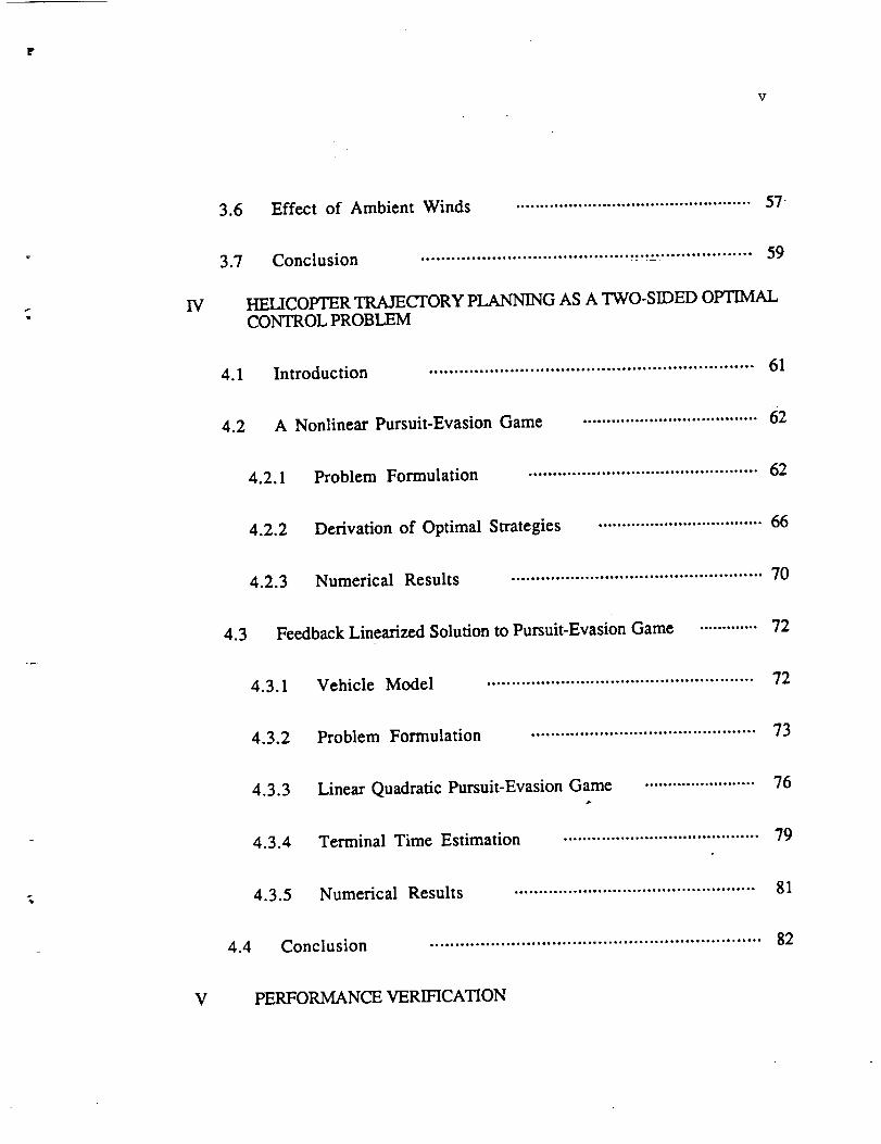
IV HELICOPTER TRAJECTORY PLANNING AS A TWO-SIDED OPTIMALCONTROL PROBLEM
4.1 Introduction OBOOB.e_*OJJ_OOO_ • IOJl,JOOO.. J,• BIO,....,.•,J•OO._,OlJaOliOIO'°" 61
4.2 A Nonlinear Pursuit-Evasion Game ..................................... 62
4.2.1 Problem Formulation • 62,me_,oo_o.lIQ.ooo io _. _16o.. • i.i .QIolooo._oll..
4.2.2 Derivation of Optimal Strategies ................................... 66
4.2.3 Numerical Results gq.te_QJJJibIQ..,°OJlJlJO_. OIIQ_OIODOJg'OQa°'QOO'I• 70
4.3 Feedback Linearized Solution to Pursuit-Evasion Game ............. 72
4.3.1 Vehicle Model OJ_t..J..OQ4QOO.g. IO._...°,O•_I..°..•JOO_I... _°.OI..°. 72
4.3.2 Problem Formulation .............................................. 73
4.3.3
4.3.4
Linear Quadratic Pursuit-Evasion Game ........................ 76
Terminal Time Estimation ......................................... 79
-e 4.3.5 Numerical Results • o. e_. °.oq. J°e.°.l e°°o e_°°.ee..i_.._._.._°._•,.. 81
4.4 Conclusion ,..ll,.6oQ.. OI•OOOQO•QI_.....OSI.°.. _........._8_.o_.°._..* ° iI.o. 82
V PERFORMANCE VERIFICATION

v±
5.1 Introduction °°°°°oJJJJoeoooooJJ.lo°w...l_it.w_I.jloJ.gofe_o_jmg_jwtt...ig 83"
5.2 Simulation Results g. JOg*l°,l°lJ°l°.°lllgl..*lg_I,,°allaJ.l...._lgjlU.°g°g° 84
VI CONCLUSIONS AND FUTURE RESEARCH
6.1 Concluding Remarks • H...,°°°°°°.°°°,°°°°°°°°°,...°.°_... .... ...°°l.gi,° 86
6.2 Future Research mllaJ_,itoooJliQoJioJQllai°oJ°°ilm°J_u_o_g_°_l_°°_lo°ooo*° 88
APPENDICES
A TANGENT PLANE AND COORDINATE TRANSFORMATION ..... 90
B NUMERICAL CONJUGATE POINT TEST .............................. 94
C SEPARABILITY OF THE HAMILTONIAN _ _S CONSEQUENCEON DIFFERENTIAL GAME SOLUTIONS .............................. 105
D CONVEXITY CONDITION FOR GLOBAL MINIMUM .............. 109
BIBLIOGRAPHY ......................................................................... 110

vii
LIST OF TABLES
Table
3.1
5.1
Digitized Terrain Data used for Trajectory Planning
Maximum Rate of Climb for Helicopter Model AH-1S
e.ae_
.................... 121
................ 122

v

_x
LIST OF FIGURES
-?;
Fdgam
3.1 The Coordinate System .................................................... 123
3.2 Flow Chart for Generating Euler Solutions .............................. 124
3.3 Sample Terrain Map of the Nassau Valley, California ................. 125
3.4 Euler Solutions for Minimum Flight Time Criterion ................... 126
3.5 Euler Solutions for Maximum Terrain Masking Criterion ............. 127
3.6 Comparison between Minimum Time Trajectory and MaximumTerrain Masking Trajectory ............................................... 128
3.7 Altitude Profiles along Different Criterion Trajectories ................ 129
3.8 Characteristic Determinant A(t) along the Trajectory A ................ 130
3.9
3.10
3.11
3.12
Characteristic Determinant A(t) along the Trajectory B ................ 131
Comparison of Performance Index along Trajectories A and B " •...... 132
Euler Solutions for Minimum Flight Time Criterion ................... 133
Characteristic Determinant A(t) along the Trajectory A ................ 134
3.13 Characteristic Determinant A(t) along the Trajectory B ................ 135
_._j'tL_.|,_!_TjO_l_l_ _h_,_ PRESC-OING PAGE BLANK NOT FILMED

X
3.14
3.15
Euler Solutions for Optimal Route Problem No.2
(¢z -- 1E05, e -- 0.001) .....................................................
Comparison between Straight Trajectory and an Optimal Route
Planning No.2 Trajectory (a = 1E06, ¢ = 0.001) ......................
136
137
3.16 Altitude Profiles along Straight Trajectory and Optimal Trajectory .... 138
3.17 Euler Solutions for Minimum Flight Time Criterion ConsideringWind Effects (u/V = 0.1) .................................................. 139
3.18 Euler Solutions for Maximum Terrain Masking Criterion ConsideringWind Effects (u/V = 0.1) .................................................. 140
4.1 Trajectories for the Pursuer and Evader (Wp = We = 0) ................ 141
4.2
4.3
Trajectories for the Pursuer and Evader (Wp = We = 1.0) ............. 142
Altitude Histories for the Pursuer and Evader ........................... 143
4.4 Trajectories for the Pursuer and Evader (Wp = We = 1.0) ............. 144
4.5 Altitude Histories for the Pursuer and Evader ........................... 145
4.6
4.7
4.8
Trajectories for the Pursuer and Evader (Wp "---0.0, We = 1.0) ....... 146
Trajectories for the Pursuer and Evader (Wp = 0.5, We -- 1.0) ....... 147
Legendre-Clebsch Test for the Pursuer and Evader .................... 148
4.9 Legendre-Clebsch Test for the Pursuer and Evader .................... 149
4.10 The Coordinate System .................................................... 150

xi
4.11 Trajectories for the Pursuer and Evader ................................. 151
4.12 Speed Histories for the Pursuer and Evader ............................. 152
4.13 Load Factor Histories for the Pursuer and Evader ..................... 153
4.14 Bank Attitude Histories for the Pursuer and Evader ................... 154
4.15 Pitch Attitude Histories for the Pursuer and Evader .................... 155
4.16 Altitude Histories for the Pursuer and Evader ........................... 156
4.17 Trajectories for the Pursuer and Evader ................................. 157
4.18 Speed Histories for the Pursuer and Evader ............................. 158
4.19 Load Factor Histories for the Pursuer and Evader ...................... 159
4.20 Bank Attitude Histories for the Pursuer and Evader .................... 160
4.21 Pitch Attitude Histories for the Pursuer and Evader .................... 161
4.22
5.1
Altitude Histories for the Pursuer and Evader ........................... 162
s,
Altitude Rate Response for Maximum Masking Trajectory ............. 163
5.2 Longitudinal Cyclic Control for Maximum Masking Trajectory ........ 164
5.3 Lateral Cyclic Control for Maximum Masking Trajectory ............. 165
5.4 Pedal Control for Maximum Masking Trajectory ....................... 166
5.5 Collective Control for Maximum Masking Trajectory .................. 167

xii
5.6 Pitch Attitude Response for Maximum Masking Trajectory ........... 168
5.7 Roll Attitude Response for Maximum Masking Trajectory ............ 169
5.8 Yaw Attitude Response for Maximum Masking Trajectory .......... 170
5.9 Altitude Rate Response for Minimum Time Trajectory ................. 171
5.10 Longitudinal Cyclic Control for Minimum Time Trajectory ............ 172
5.11 Lateral Cyclic Control for Minimum Time Trajectory .................. 173
5.12 Pedal Control for Minimum Time Trajectory ............................ 174
5.13 Collective Control for Minimum Time Trajectory ...................... 175
5.14 Pitch Attitude Response for Minimum Time Trajectory ............... 176
5.15 Roll Attitude Response for Minimum Time Trajectory ................ 177
- 1
5.16 Yaw Attitude Response for Minimum Time Trajectory ............... 178

xiii
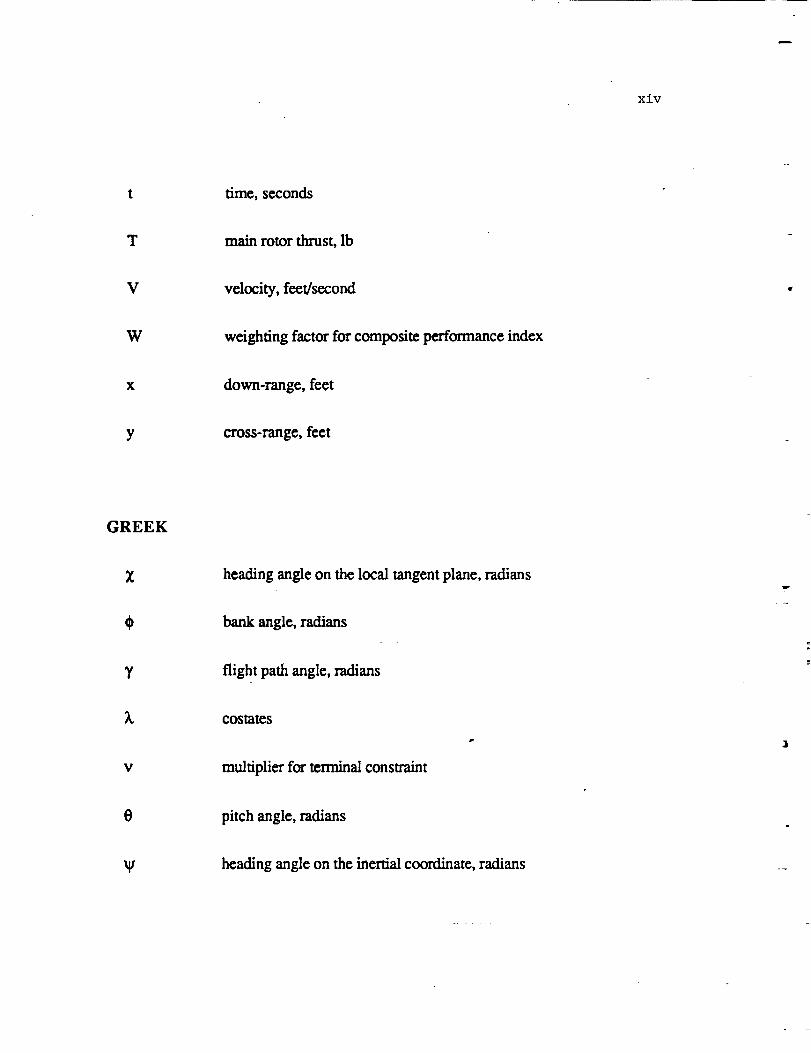
LIST OF SYMBOLS
ALPHABET
d radius of the capture set, feet
f(x,y) terrain altitude, feet
g gravitational acceleration, feet/second 2
h altitude, feet
H variational Hamiltonian
performance index, payoff, cost function
K weighting factor for composite performance index, 0 < K _<1
m helicopter mass, slugs
P terminal constraint
?. 9_ real number
R initial constraint
S switching function
xiv
time, seconds
T main rotorthrust, lb
V velocity, feet/second
W weighting factor for composite performance index
x down-range, feet
Y cross-range, feet
GREEK
Z
3'
heading angle on the local tangent plane, radians
bank angle, radians
flight path angle, radians
w
V
costatcs
multiplier for mnninalconstraint
0 pitch angle, radians
V heading angle on the inertial coordinate, radians

xv
SUBSCRIPTS
clearance between helicopter and the terrain
-e evader
f terminal time
local coordinate system
0 initial time
P pursuer
SUPERSCRIPTS
a augmented
T transpose
o optimal
ACRONYMS
ARMCOP A single main rotor helicopter simulation program (U.S. Army)
E-L Euler - Lagrange
HELCOMP A helicopter air - to - air combat simulation program

xvi
_UB Hamilton - Jacobi - Bellman
L-C Legendre - Clebsch
LHX Light Helicopter eXperimental
NOE Nap - of- the - Earth
ORP Optimal Route Planning
P.I. discreet Performance Index
TMAN 6 DOF helicopter simulation program (NASA Ames Research
Center)
TPBVP
WKB
Two Point Boundary Value Problem
Wentzel - Kramers- BriUouin
F

xar±±
SUMMARY
Helicopters operating in high threat areas have to fly close to the earth surface to
minimize the risk of being detected by the adversaries. This report presents techniques for
low altitude helicopter trajectory planning. These methods are based on optimal control
theory and appear to be implementable onboard in realtime. Second order necessary
conditions are obtained to provide a criterion for finding the optimal trajectory when more
than one extremal passes through a given point. A second trajectory planning method
incorporating a quadratic performance index is also discussed. In a later part of the thesis,
trajectory planning problem is formulated as a differential game. The objective here is to
synthesize optimal trajectories in the presence of an actively maneuvering adversary.
Numerical methods for obtaining solutions to these problems are outlined. As an
alternative to numerical method, feedback linearizing transformations are combined with the
linear quadratic game results to synthesize explicit nonlinear feedback strategies for
helicopter pursuit-evasion. Some of the trajectories generated from this research axe
evaluated on a six-degree-of-freedom helicopter simulation incorporating an advanced
autopilot. The optimal trajectory planning methods presented here are also useful for
autonomous land vehicle guidance.


CHAPTER I
INTRODUCTION
1.1 Introduction
Recent years have seen an increased interest in helicopter operations near the ground as
evident in the literature [1-3]. In a high threat environment, helicopters have to fly close to
the earth surface to minimize the risk of being detected by the enemy [4-5]. The objective
here is to use terrain and surrounding objects to mask the helicopter during the mission.
Due to data processing limitations, a hierarchical system architecture is essential for
nap-of-the-earth flight guidance. This concept provides a natural way of decomposing a
complex control process into simpler and more manageable components. Thus, the
guidance functions are divided into three levels, namely, far-field, mid-field, and near-field
[6].
The far-field planning task involves off-line mission planning to generate mission
way-points and goals. Mission requirements, global threat information and vehicle
resources on-board are taken into account. The mid-field planning function generates the
flight route using the way-points data given by the far-field planner. High resolution digital
map, threat information, and vehicle limitations are included in performing real-time
guidance computations. The near-field guidance function provides a least expected
deviation path from the mid-field nominal path due to the vehicle dynamics limitations and

2
obstacles detected by on-board sensors. The focus of this report will be on the mid-field
route planning problem.
Most route planning methods given in the literature [7-11] appear to use the terrain
altitude and lateral deviations from a nominal trajectory as the performance index. These
methods are based on the heuristic search techniques including variants of dynamic
programming such as the A*-algorithm. All these approaches employ the discretization of
the terrain spatial coordinates before carrying out a systematic search for optimal trajectory.
On a rough terrain, these approaches require an enormous amount of computation and
storage to generate sufficiently smooth trajectories [12].
An alternative formulation for the trajectory planning is based on Pontryagin's
maximum principle and was first outlined in Reference 13. State equations in this
formulation include the terrain constraint, incorporated via a coordinate transformation.
The performance index is a linear combination of flight time and terrain altitude. The
resulting nonlinear two-point boundary value problem is then converted to a one-
dimensional search process by incorporating a constant of motion and employing an
adjoint-control transformation. The solution is implementable in near real time and is
capable of detecting situations where more than one extremal passes through a given point.
The second-order necessary condition for this problem is studied in detail. This trajectory
planning method automatically accomplishes known-threat avoidance and is similar to the
classical Zermelo's navigation problem [14]. In this method, the computationifl algorithm
requires the second partial derivatives of the terrain profile to generate extremals. As a
result, the terrain prof'fle needs to be represented by quadratic or cubic splines lattices. This
feature can sometimes make the extremals sensitive to the error in the terrain data.
In an alternative formulation [15], the need for second partial derivatives is eliminated
by avoiding the coordinate transformation approach. The performance index in this
2.

3
problem consists of a quadratic form in the terrain altitude, lateral deviation from the
nominal trajectory, and heading angle. By changing the independent variable from time to
down-range, the order of the problem is reduced. As in the first method, the extremals are
obtained using the optimal control theory and necessary conditions are tested along the
extremals. An approximate second variation test is developed for this problem using the
WKB method [16]. A special case that can result in singular arcs in this trajectory planning
problem is also outlined.
So far, the route planning problem for single vehicle has been discussed. As a natural
extension, the guidance for two or more vehicles that cooperate or compete against each
other is considered next. This results in a differential game formulation for the trajectory
planning problem. Since the publication of a book by Isaacs [17] on differential games in
1965, a body of research is available on differential games with kinematic models in a
plane. With such simple modeling, it is possible to obtain elegant results. The well-known
homicidal chauffeur problem is an example. On the other hand, the helicopter guidance
problem requires the use of a model in which the coefficients vary as a function of the
vehicle position on the terrain. The method proposed in this report uses the terrain profile
data to formulate a differential game between two helicopters.
In conjunction with the recent theory of nonlinear transformations, Menon [18]
showed that a class of differential games with nonlinear dyn_aics can be transformed into
the well known linear quadratic pursuit-evasion game form. Compared with the previous
derivations of pursuit-evasion guidance laws which completely ignore the dynamic
nonlinearities in the vehicle models, the nonlinear transformation approach continuously
compensates for the vehicle nonlinearities. In the present work, this formalism is used to
study a helicopter pursuit-evasion game at nap-of-the-earth flight altitudes.

4
Finally, in order to verify whether the trajectories generated using various planning
schemes discussed in the foregoing satisfy the helicopter physical constraints, these need to
be evaluated on a detailed helicopter simulation. An advanced autopilot developed by
Heiges [19] together with a six-degree-of-freedom helicopter simulation is used in this
investigation. The helicopter simulation was originally developed at NASA Ames Research
Center for the study of Air-to-Air combat [20-21].
1.2 Contributions of the Reoort
In contrast with the existing literature, this report develops techniques for trajectory
planning based on the Calculus of Variation. Numerical algorithms are given for the
determination of optimal trajectories with various performance indices. Additionally, tests
are developed for verifying the optimality of the emerging trajectories.
Methods deveioped in the present research will aid in constructing an integrated
methodology for low altitude flight guidance of helicopters. The trajectory planning
solution is also useful for autonomous surface/underwater vehicle guidance, terrain
foUowing guidance for cruise missiles and aircraft [22-24] and optimal trajectory planning
for robots.
w
1.3 Organization of the Renortv
This report is organized as follows:
Chapter II gives a brief description of previous research on helicopter low-altitude
flight trajectory planning and air-to-air combat. It was the work in this area that motivated
the present research topic. This chapter also covers a few well-known results in optimal
z

5
control theory and differential game theory. Background on the nonlinear transformation
techniques to control nonlinear systems is also presented.
Two optimal trajectory planning schemes useful for the terrain-following/terrain-
avoidance guidance of helicopter are presented in Chapter 11I. This chapter illustrates how
the nonlinear two-point boundary value problem can be solved using a one-dimensional
searching method. To ensure that the extremals obtained by this approach are optimal,
second-order necessary conditions are also developed in this chapter.
In Chapter IV, research on the helicopter pursuit-evasion is discussed. A backward
integration method and a nonlinear transformation method are given in this chapter.
Chapter V discusses the implementation and test of the generated trajectories in a
realistic six degrees of freedom helicopter simulation. The helicopter physical variables
along the trajectories obtained from Chapter Ill are examined here.
Chapter VI evaluates the results obtained from present research. Suggestions for
future work are also outlined.
Finally, the appendices contain some of the analysis used in the main body of the
report. In Appendix A, the transformation from local tangent plane to inertial coordinates is
derived. This transformation is employed in developing the first trajectory planning
scheme (ORP #1). Various numerical conjugate point tests and their relationships are
discussed in Appendix B. These tests are used to verify the optimality of the synthesized
trajectories. In Appendix C, separability of the Hamiltonian and its consequence on
Differential Game solutions are discussed. A necessary condition for global minimum is
given in Appendix D.
All numerical results are obtained with VAX-11/750 TM. Contour maps are drawn by
DISSPLA TM graphics routine. Algebraic equations are derived by symbolic program

6
MACSYMA TM. Unless otherwise mentioned, British Units, i.e., pound (Ib) - foot (ft) -
second (sec), arc the basic units used in this report.
w

7
CHAPTER II
BACKGROUND
2.1 Introduction
In this chapter, previous research on the helicopter trajectory planning problem and air-
to-air combat are reviewed. An overview of Dynamic Programming used in several of
these research is given in Section 2.4. This section also provides an outline on optimal
control theory. Section 2.5 provides a review of several notions involved in differential
games. Finally, some recent results in nonlinear transformations for feedback control are
reviewed in Section 2.6.
2.2 Previous Research on Helicopter Trajectory Planning
p.
Historically, terrain information has been used for low altitude flight guidance of deep
penetration attack aircraft and cruise missiles. Since these vehicles fly a consiclerable time
over the opponent's territory, they are vulnerable to detection by the enemy. The objective
of low altitude flight guidance using terrain map is to minimize the influence of air defense
threats on the mission profile [25-26]. Trajectory generated by such a guidance scheme is
composed of a terrain-following path in the vertical plane. In the nap-of-the-earth guidance
of helicopters, on the other hand, both vertical and lateral maneuvers are employed.

8
Reference 7 discusses the computation of vertical and lateral helicopter trajectories
using a combination of discrete dynamic programming [27] and tree searching [28]. They
considered the performance indices for the lateral and vertical planes as follows:
JL = _ [wD_i + (hcl + Hi) 2] (2.1)i
Jv = _ (hcl + Hi) 2 (2.2)i
where, w is the terrain-following/terrain-avoidance ratio, Di the lateral deviation from
reference path, Hi terrain altitude at location index i, and he1 helicopter clearance altitude.
Note that the two performance indices do not include control terms.
Reference 11 developed an algorithm to generate a low altitude threat penetration
trajectory which minimizes the performance index:
J - _ (Di + COAti (2.3)i
<
Here, Di is the value of the danger array at the ith cell, Ati the transition time, and Ct the
cost of time. Danger arrays Di depends on the vehicle position (x,y,h), and the heading
angle Z. Ct is a coefficient including flight time and fuel. Decoupled vertical and lateral
threat penetration trajectories were obtained by dynamic progamming and tree search.a.
Reference 29 describes a three-dimensional dynamic programming approach to
maximize the overall probability of survival Ps along any path defined by: ,
v.-- 1] P (x,y,zj)path (2.4)
where, Ps(x,y,z,j) is the probability of survival through cell (x,y,z) in the jth direction to an
adjacent cell. In the actual implementation, the values assigned to each cell are negative
logarithms of the probabilities of survival. The problem is thereby transformed from one
W
]

9
of maximizing the product of survival probabilities to minimizing the sum of negative
logarithmic probabilities. The probability is a function of terrain masking, fuel constraint,
or time constraint.
The investigators in artificial intelligence area [10] have suggested to use the heuristic
search to find a near-optimal routes for autonomous helicopter. Two of the most
commonly used heuristic search techniques for finding optimal path are the branch-and-
bound and the A*-algorithm, discussed in Reference 10. The branch-and-bound is an
exhaustive search method similar to both depth-f'urst and breadth-f'trst schemes. They
search all possible paths until the goal is found. A*-algorithm is the branch-and-bound
search in conjunction with the dynamic programming principle to reduce computations
[28].
All these approaches employ the discretization of the terrain spatial coordinates before
carrying out the search for the optimal trajectory. As a result, they assume that the route
consists of straight line segments. On an uneven terrain, this implies that a large number of
discretization intervals will be required to generate sufficiently smooth trajectories.
Unfortunately, this increase in the number of discretization intervals is accompanied by an
enormous increase in computational complexity. For example, in the case of discrete
dynamic programming, this is of order {(n+l):+I}, where n is the number of
discretization intervals in one spatial direction [12]. A solution advanced by some
researchers for handling this "curse of dimensionality" is the use of parallel-computing
architectures [30].
This report will propose alternative trajectory planning schemes based on the Euler-
Lagrange equations [12]. These approaches require a one-dimensional search to detemaine
optimal trajectories. Further details will be discussed in Chapter M.
ii
10
2.3 p rgvious Research on Heliconter Pursuit-Evasion
Unlike the one-sided trajectory planning problem, reported research on two-sided
trajectory planning has been very sparse. A previous research [31] employed a discrete
matrix game approach for generating maneuvering decisions for low altitude flying
helicopter during one-on-one air combat over a hilly terrain. Each player had seven
maneuvering strategies, and thus the game matrix consisted of 49 payoff elements. Each
element in this matrix represented the score evaluated using a scoring function. Under the
perfect information assumption, the scoring function was composed of an orientation, a
relative range, a velocity, and a terrain profile. The state variables required in evaluating
the scoring function were obtained by numerically integrating the equations of motion for
each of the seven strategies of the participants. After numerical integration, the saddle point
was searched and optimal maneuvering strategies for each player were obtained. This
procedure was repeated until terminal conditions are satisfied.
According to Von Neumann and Mongenstem [32], every finite and discrete game can
be cast in the matrix form. However, the dimensions of this matrix will be astronomical
except for very simple problems. Additionally, the computational effort in conducting a
search for the optimum can be prohibitive. R. Isaacs [17],provided the framework for
obtaining solutions to continuous games with differential constraints. This will be further
elaborated in Section 2.5.
In this report, the helicopter pursuit-evasion problem will be studied as two one-sided
optimal control problem using differential game theory. Two different formulations will be
discussed. The first one requires two-dimensional search to determine optimal strategies.
Another approach using nonlinear transformation techniques demands the specification of
the terminal time. Details of these approaches will be given in Chapter IV.
v

11
2.4 A Review of The Ontimal Control Theory
In order to motivate subsequent development, this section will present a review of the
central results from optimal control theory [12].
Given the state equations:
_t= f(x,u,t), x(to)= x0 (2.5)
where, x(t):= statevectorof dimension n,x • X
u(t):= controlfunctionofdimension m, u ¢ U
Initial constraints:
R (X(to),t0 = 0
Terminal constraints:
(2.6)
P (x(tt),tf)= 0 and tfisfree (2.7)
Performance Index:
[u] = g(x(tf),tf)+ J L(x,u,t) dtJ
to(2.8)
The optimal control problem is to pick u(t) to minimize J[u] while satisfying the state
equations and the boundary constraints.
The optimal control can be obtained using Dynamic Programming [27] or Pontryagin's
Minimum Principle [33]. For most problems encountered in applications, these two
approaches can be shown to be equivalent [12].

tim
12
2.4.1 Continuous D_,namic Programming
Define thecontinuousoptimalreturnfunctionas
J°[x(t),t] = rain J[x(t),u(t),t]ueU
(2.9)
To simplify presentation, it is assumed here that the terminal cost is zero. Next, assuming
the optimal return function to be continuous, one can write [34]
t+_ _f
J°[x(t),t] = rain {f L(x,u,x)dx + f L(x,u,x)dx } (2.10)ueU
t t+E
for sufficiendy small E. If the vector functions u(x) and L are both continuous at t, there
exist an E sufficiently small such that expression (2.10) can be approximated as:
|f
J°[x(t),t]= rain {eL(x,u,x) + S L(x,u,'c)dx } (2.11)u_ U t+t_
w
From the definition of jo the optimal remm function (2.9), this amounts to
J°[x(t),t] = rain {eL(x,u,t) + J°[x(t+e),t+e] }. (2.12)ueU 2
The state evolution may next be approximated by
x (t+e) = x(t) + lff(x,u,t) (2.13)
Substituting equation (2.13) into (2.12), for sufficiently small positive E, and retaining only
the first-order terms, one has

13
o
J°[x(t),t] = rain {eJ.,(x,u,t) + J [x(t)+ef(x,u,t),t+e] } (2.14)uCO
Taking a Taylor's series expansion of J°[x(t)+ef(x,u,t), t+E], and retaining only the first
order terms,
j°[x(t)+ef(x,u,t),t+e] = J°[x(t),t] + r_x[x(t),t ] f(x,u,t) + e _[x(t),t] (2.15)
Next, substituting (2.15) into (2.14), and cancelling the J°[x(t),t] term and dividing by e,
one has
oJt[x(t),t] = - rain { L(x(t),u(t),t) + fx[x(t),t] f(x,u,t)} (2.16)
u_U
Let u ° (x,t) denote the optimal control given x and t. This control must yield a minimum
for the fight hand side of equation (2.16). Thus,
[x,t] = - L(x,u*,t) - _ [x,t] f(x,u*,t) (2.17)
Equation (2.17) is known as the Hamilton-Jacobi-Bellman (I-IJB) equation. This is a first
order nonlinear partial differential equation.
This equation is difficult to solve if the functions L and'f are highly nonlinear. As a
result, this equation is often solved using the method of characteristics. The characteristics
of the HJB equation are called the Euler-Lagrange (E-L) equations [12]. The E-L equations
are first order nonlinear ordinary differential equations with prescribed boundary
conditions. In the following we will indicate the derivation of E-L equations using the HJB
equation.
14
Differentiating the expression (2.17) partially with respect to x, and noting that the
control variables are independent of the state variables results in the expression
J*,.[x,t] = - L_(x,u*,t) - J*n[x,t] f(x,u*,t) - f_(x,u*,t) _[x,t] (2.18)
Now, the total derivative to J*x[x,t] is given by
d._[x,t] = _,[x,t] + _,[x,t]f(x,u*,t)dt (2.19)
Substituting (2.18) into (2.19), one has
d_[x,t] =- Lx(x ' uO' t)-dt fx(x, u°, t) _x[x,t] (2.20)
O
This set of fh'st-order ordinary differential equations for Jx [x,t] can be solved if x and u °
were known for all t and initial conditions for o oJx [x,t] areJx [x,t] were given, called the
costatesof the systems, often den0ted by the variable _ .......
2.4.2 Pontrva_in's Minimum Principle
Introducing a new variable called the Hamiltonian [12],
H (x,u,_.,t) = L (x,u,t) + XT f (x,u,t) (2.21)
3,
The Euler-Lagrange equations (2.5), (2.20) can be written as
= f(x,u,t), (2.22a)
_. = - H x (2.22b)
15
The fact that optimal control u has to minimize the quantities within braces in (2.16) leads
to the so called optimality condition
Hu = 0 (2.23)
Equations (2.22) must satisfy the given boundary conditions. For additional details on this
problem, see Reference 12.
While the satisfaction of HIB is sufficient for optimality, additional conditions must be
imposed while solving the optimal control problem using the E-L equations. In this case,
the optimal controls emerging from (2.22), (2.23) should additionally satisfy the following
condition [ 12]:
(i) Legendre-Clebsch condition
Huu>_0 (2.24)
(ii) Weierstrass condition
_H (x, _.o, uo, u, t) > 0 (2.25)
Off) Jacobi condition
Nonexistence of conjugate point in (t0,tf)
Conditions (i) and (iii) are necessary for weak local minimum, while condition (ii) is
necessary for strong local minimum. Strengthening conditions (i) and (ii) and closing the
interval in condition (iii) constitute the sufficient condition [12]. In some situations,
normality condition [12] has to be verified before testing the conditions (i) - (iii).

I
16
Additional conditions can be obtained using various combinations of these necessary
conditions [35].
2.5 A Review of Differential Games
If optimal control theory briefly reviewed in the previous section can be considered a
theory for one-sided control problems, differential game theory may be identified as a
theory for two-sided control problems. It has been shown [36] that the problem definitions
and solution methods used in optimal control theory can be extended into the game theory.
The theory of differential games is a subject concerned with the optimization of
dynamic systems involving two or more players with conflicting interests. The study of
differential games was initiated by Isaacs in 1954. In 1965, Isaacs published a book which
details various aspects of differential games [17]. In 1957, Berkovitz and Fleming [37]
solved a simple differential game using the calculus of variations. In a later research,
Berkovitz treated a wider class of differential games using the calculus of variations [38].
Friedrnan's book [39] discusses the necessary conditions in differential games in terms of
the more familiar optimal control theory notation.
The aforementioned differential games mostly dealt with problems of the pursuit-
evasion type having the zero-sum property, i.e., one player's losses.being the other player's
gain. Dropping_the zero-sum hypothesis a_s both conceptual and analytic complexity, but
it may extend the utility of the theory of differential games to a much wider class of
applications. Two typical non-zero-sum games are the Nash game and Stackelberg game,
in which each participant has its own performance criterion.

17
Assuming that the players have perfect information of the current states and that their
respective roles are determined before the game begins, a differential game may be stated as
follows: -
Given differential constraints:
- f (x,¢,V,t), x(t0)=x o (2.26)
where, x(t) : = state vector of dimension n, x • X
¢(0 : = control of Player 1 of dimension e, ¢ e •
ag(t) : - control of Player 2 of dimension m, _ •
Initial constraints:
R (xCto),to) = 0
and terminal constraints:
(2.27)
P (x(tf),tf) = 0, tf is free (2.28)
The terminal constraints define the stopping condition for the game. For example, if the
participants have a "capture set", the game terminates at the instant the adversary enters the
capture set.
The performance index or payoff for the i th player may be defined as
F
Ji[x,_,¥,t] - gi(x(tf),tf ) + Li(x,_,lg, t) lit (2.29)
Each player involved in the game attempts to optimize its own performance index with due
attention to the other player's state-control variable evolution. Once the differential
constraints, initial and terminal constraints and the performance index are defined, one may
describe three different game scenarios.

18
Hi"
2.5.1 Nash Non-Zer0-Sum Game
If an optimal solution exists, optimal closed loop control pair ($o, vo) must satisfy the
Nash incqua_ties condition [40]:
J2(_°,'¥ °) g J2(_,'¥°), V Ce ¢I)
(2.30)
(2.31)
Inequalities (2.30) and (2.3 I) imply that optimal strategies for each player should yield the
smallest cost for individual participants. Any deviation from the optimal su'atcgy will yield
a higher cost.
2.5.2 StackelberlL Non-Zero-Sum Game
Inthisgame, one assumes thatthesecondplayeristheleaderwhilethefirstplayeris
thefollower.As a result,thefirstplayerisoperatinga purelyreactivefashion.Ifthere
existsa mapping M:_ ---->_, and thefollowingconditionsarcsatisfied,thenthepair(_b*,
V*) • q)x _Piscalleda StakclbcrgstrategypairwithPlayer2 as a leaderand Playerl as
follower[41]:
JI(M_, _) -<Jl((_, V) (2.32)
J2((_*, _) -<J2(M_I/,V) (2.33)
_b*= M W* (2.34)
In otherwords,theStackelbergstrategyistheoptimalstrategyfortheleaderwhen the
followerreactsby playingoptimally.An interestingpropertyrelatingthe Nash and
Stakelbergstrategiescan be derivedfrom equations(2.30)-(2.34)asfollows[41]:

19
* j oJ2({_ , _*) _ 2(_b , _o) (2.35)
which means that the leader in the Stackelberg solution achieves at least as good a cost
function as the corresponding Nash solution.
2.5,3 Zero-Sum Game
Zero-sum games resultwhen thetwo decision-makersareadversaries.One decision-
maker'slossistheotherdecision-maker'sgain.In thiscase,theequilibriumsolutionhas
thepropertythat
J1 -- -J2 - J (2.36)
The above Nash inequalities criterion (2.30) and (2.31) may be reduced to
o o oJ [x,¢°,V,t] ___J [x,¢ ,V ,t] _< J [x,¢,_ ,t] (2.37)
where, J [x,¢°,V°,t] -=V [Xo,to] is called the value of the game. In such a differential game
both players have the same performance index, with the first player minimizing it while the
second player attempts to maximize. Equation (2.37) suggests that if the minimizing player
deviates from his optimal strategy, the game will have a higher game value. Alternatively,
if maximizing player deviates from the optimal strategy, the game will have a lower value
than if the two were employing optimal strategies. This is the well-known saddle point
condition in the game theory [32]. A similar saddle point condition may also be derived
from the Stackelberg inequality conditions.
Introducing the variational Hamiltonian
H (x,¢,%X,t) = L + XT f (2.38)

i
20
and define the terminal conditions as:
Q(xCtf),tf) = g(x(tf),tf) + v T P (x(tf),tf) (2.39)
Since _t = f(x,u,t), one may write the performance index as
firj t __Q(x(tr),tf) + (H - xT_t) dt
Jto
(2.40)
Since the control terms appear only in the function H, the saddle point condition (2.37) can
be written as [42].
H(x,t_ ,V,_L,t) dt < H(x,0 ,xlt°,_.,t) dt< H(x,¢,gt°,2L,t) dt (2.41)--dll
If for all t, functions L and f arc continuous, the inequality (2.41) can be changed to
the pointwise form [42] by using the principle of optimality which requires that at every
instant controls should be chosen to make system optimal:
O O
H(x,¢ ,V,2L,t) < H(x,¢ 0g°,2k,t) < H(x,¢,q/°,_.,t) (2.42)
Equation (2.42) is a sufficient condition for the inequality (2.41) and a differential game
version of Weierstrass condition in the optimal control.
Generally, by the order of action it is known [35] that
max rain H(x,q,_,_t) = min max H(x,t),¥, X, t) (2.43)¥ ¢ ¢ ¥
.I

21
Additional conditions sufficient for satisfying the above equation (2.43) as equality for a
special case was given by Von Neumann and Morgenstem [32]. This is known in the
literature as the Isaacs principle.
If H is separable in 0 and _, i.e.,
f(x, ¢, V, t) = fl (x, t_, t) + f2(x, V, t) (2.44)
L(x,¢,_l/,t) = Ll(X, ¢, t) + L2(x, _,', t) (2.45)
it may be shown [39] that
max rain H(x,¢,V,X,t)= rainV ¢ ¢
max H(x,0,¥,X,t) = H(x,¢°,V°,_.,t)¥
(2.46)
Since the stationarity conditions (first-order necessary conditions) are the same for
minimization or maximization, the differential game can be def'med as a two-sided optimal
control problem with coupling appearing via the transversality conditions. In this case, the
necessary conditions for ¢(t) and V(t) to be optimal are:
1) Euler-Lagrange equations
x = f(x,¢,V,t)
_-- - Hx
2) Transversality conditions at tf
_,'r(tf) = Qx(x(tf),tf)
(2.47)
(2.48)
(2.49)
P (x(tf),tf)= 0 (2.50)

m
22
H(tf) = 0, tf is free (2.51)
3) Optimality conditions
He=0 (2.52)
Hv= 0 (2.53)
4) Isaacs principle
max rain H(x, ¢, V, X, t) = rain max H(x, 0, _t, X, t)¥ , ¢ ¥
(2.54)
It may be shown that this solution can be also obtained by solving a partial differential
equation similar to the HIB equation [39]. In the differential game context, this PDE is
called the Hamilton-Jacobi-Isaacs equation for the optimal J [39], viz,
O
Jt (x,t)=- rain max H(x,¢,_,J°,t) (2.55)J
J°(x(tf),tf) = g(x(tf),tf) (2.56)
The similarity of the differential game and optimal control is apparent from the
foregoing. However, it is important to note that certain differences exist between optimalF
control problems and differential games [43]. First, although feedback control is not
essential in the optimal control problems it becomes the central requirement in" differential
games. Secondly, the solution is characterized by regions where solutions exist and where
they do not. Moreover, verification of the second-order necessary conditions, while not
routinely employed in optimal control, becomes mandatory in differential game solutions.

23
2.6 Transformation Qf Nonlinear Systems
Even though differential game theory has several potential applications in economics,
military, and engineering, it has not been employed to the same degree as optimal control
theory. However, linear-quadratic differential games have received considerable interest in
the differential games literature [40, 41, 43, 44]. These games have been important in
studying the local behavior of certain nonlinear differential games. Recently, it has been
shown that a class of nonlinear differential games may be solved in closed form using
transformations [18]. In that work it was shown that nonlinear transformation techniques
are useful for implementing linear-quadratic differential game solutions in nonlinear
differential games.
2.6.1 Kronecker lnflices and Brunpv_ky Fornl
Before tackling the nonlinear system control problem, a brief review of linear system
theory in the state space will be given. For a given multivariable system
r,(O = A x(O + B u(t), x e _n, u e ¢Xrn (2.57)
the first step in designing control laws is to test for controllability.
computation of a controllability matrix C{A, B } [45] as
Ibl,Abl, A2bl, ....Akrlbl, b2, Ab2, .......,Ak=-IbmlI
This involves the
(2.58)
For the system to be controllable, this matrix must have a rank n [45]. Next, this matrix
may be normalized to determine a transformation matrix
T= {ell, el2, .... elkt, e21, ...... eml, .. emkm} (2.59)

m
24
or,
Defining a new set of state variable x = Ty and substituting in (2.57), one has
y = T-1AT y + TqB u (2.60)
with
y = Ac y + Bc u (2.61)
Ac=TqAT , Bc =TqB
Under this transformation the matrices Ac and Bc will have mostly zero or one entries
together with a specific structure.
"0 • • @ • • • 00
10000
01 O0 000
O0O0O00
000A =
c 000
000
000
.00 0
where symbol • means any
invariant parameters are
For example, n=lO, m=3, k1=3, k2=3, k3---4
• " "1 • •
o0000 0 0 0
O0 000
0. 01,
000
B© = 0 0 0 (2.62)O01
000
000
.0 O0
numeric entry. In this controller canonical form, the canonical
0
1 000000
01 00000
@ • • • 0@ 0
0001000
0 0001 O0
0 000 01 O.
k i o[j} "(2.63)
where, ki is called the controllability indices, or Kronecker indices and o_jeigenvalues of
system.
Using control law
u(t) = G v(t)- K y(t) (2.64)
the system (2.61) becomes

25
3_= (A,-B.K) y + B,G v (2.65)
By suitable choice of input transformation G and state feedback gain K, the entries marked
* in the {lst, (kl+l)st, (kl+k2+l)st ..... } rows of Ac and Bc can be zeroed out to get the
special controller form as follows:
= A"y + B"v (2.66)
For the aforementioned
_ ...
example (2.62),
"0 00 00 0000 0-
1 0 0 0 000000
0 1 0 0 000000
00 0 0000000
00 0 1 000000
00 0 0 1 00000
00 0 0 000000
000 0 001 000
0000000100
O0 0 0 00001 0
1 00
000
000
0 10
000
000
00 1
000
000
000
(2.67)
As we can see in (2.67), all eigenvalues of system can be zeroed out. The only
remaining invariants are the Kronecker indices. This special controller canonical form is
called the Brunovsky canonical form [45] and exhibits a parallel array of m decoupledD,
subsystems of dynamic order kl, k2, k3, .... ,km [46].
2.6.2 Nonlinear Transformation
In the differential geometry, the Brunovsky canonical form can be viewed as a group
acting on the space of linear systems. Each subsystem forms a single orbit under the group
action and new system pair {A*, B*} are cyclic (single-companion-matrix). Such
differential geometric concepts in linear control theory have been extended into nonlinear

E
26
systems with control variables appearing linearly m the dynamics by Krener [47] and
Brockett [48]. An infinitesimal group theory and tangential transformations for nonlinear
differential equations studied by Marius Sophus Lie [49] forms the basis for transforming a
nonlinear system to linear system. Compared with the usual linearization using a Taylor
series expansion about a fixed equilibrium point, local tangential transformations expand
Taylor series continuously along the trajectory.
carries its convergence house with it [50].
Consider the nonlinear system
m
= f(x) + E gi(x)ui(t)i=l
Thus, the approximation, like a turtle,
(2.68)
where x, fix), gi(x) are n vectors with the hypothesis that f(0) = 0, causality condition, and
u are the m control variables. This system may be transformed to Brunovsky's canonical
form using two distinct approaches. Each of these are discussed below.
2.6,2.1 Hunt & SuiS Afibroach
References 51 and 52 showed that the transformation T = (T 1, T2, .... , T n, "In+1......
Tn+m) is required to have the following properties
(i)
(ii)
f_)
(iv)
(v)
T (0) - 0.,P
T 1, T 2, .... , T n axe functions of x l, x2...... xn.
Tn+l, Tn+2, .... , Tn+m, are functions of x 1, x2, .... , x_,u 1, u2..... , um.
T maps the open set U of _Rn into 9_n with a nonsingular Jacobian matrix.
T 1, T 2,.... , T n are the state variables and Tn+ 1, "In+2, .... , "In+m are the controls
for a linear time-invariant system in the Brunovsky form.
Reference 53 gives necessary and sufficient conditions to map to the Brunovsky form
with m Kronecker indices _q, _:2...... r,_m. Because the Lie bracket operation on pairs of

27
vectors keeps invariant characteristics independent of the choice of coordinate systems
used, introduce the Lie brackets
If'g] - f - _x g (2.69)
where bg/_x and 3ff0x are n x n Jacobian matrix. One may define an alternative notation to
simplify the analysis. Thus, let
if, g] = (adlf, g) (2.70)
Successive Lie Brackets can then be expressed as
g = (ad°f,g)
[f,g]= (adlf,g)
[f,[f,g]]=(ad2f,g)
[f,(ad2f, g)] = (ad3f, g) (2.71)
[f,(ad"If,g)] = (adnf,g)
The transformation T = (T 1, T2...... T n, Tn+l, .... , Tn+m) exists if and only if#-
(i) the set C = {(ad°f, gl), (adlf, gt), ..... (ad_llf, gl), (ad°f, g2), (adlf,g2) ..... ,
(adX2-1f, g2), .... , (ad°f, gm), (adtf, gm), .... , (adrm'lf, gm)} spans R n about the origin.
(ii) the sets Cj = {(ad°f, gl), (adlf, gl), ..... (adZj2f, gi), (ad°f, g2), (adlf, g2) ......
(ad_Cj-2f,g2) ...... (ad°f, gm), (adlf,gm) .... , (adtrj'2f, gm)} are involute for j = 1, 2 ...... m.
(iii) the span of each Cj is equal to the span of Cj n C.
m
28
By def'mition, a linearly independent set of vector fields {x 1, x 2, ..... Xn} is involute ff and
only ffthereare scalarfunctionsoqjksuch that
II
[x i, x j] = 5". aij k x k for all i,j,k (2.72)k=l
2.6.2.2 Mever's Avnroach
This approach is more intuitive. In this technique, the states to be controlled arc
successively differentiated until control terms appear in the equations. Various steps during
thesedifferentiationsform themapping.
2.6.2.3 Comnarison of Two Avnroaches
Although Hunt and Su's approach is more systematic than Meyer's, it is nearly
impossible to solve partial differential equations for T-transformations except in very
simple problems. Meycr's approach is a special case of Hunt and Su's approach.
If system equations arc derived by the classical dynamics with forces and moments as
control variables, then control terms will appear in the second-order kinematic equations.
In this case, Meyer's approach can be easily implemented and the transformed system is
always a double integrator system. This technique has been used in Robotics for several
years and called the Computed Torque Method.
For comparisons, a simple example is provided by the problem of a verticklly moving
vehicle of unit mass which has thrust u and drag being proportional to the square of the
speed. The equation of motion can bc written
= - G - K_2+ u (2.73)
with G denoting gravity. In state variable form, the system can be expressed as follows:

29
_1 -- X2
_2 =- G- Kx_+ u
In the standard notation (2.68), it can be expressed as follows:
(2.74)
(2.75)
(2.76)
First, consider Hunt and Su's Method.
that rank {g, [f,g]} -2 and that {g, [f,g] } be involute. It is easy to check that
[f,g] = 0 - [
Ig, [f,g]l =[
The necessary and sufficient conditions are
0 1 1 (2.77). .2Kx 2 j
0 - 1 ]= I # 0 (2.78)1 2Kx 2 I
which has rank 2 and the vector field { g, adf(g)} is involute.
with writing a Brunovsky form
Then, the method begins
(2.79)
where
Yl = Tl(Xl,X2)
Y2 = T2(xl,x2)
v = T3(xx,x2,u)
(2.80)
(2.81)
(2.82)
From Brunovsky form,
m
3O
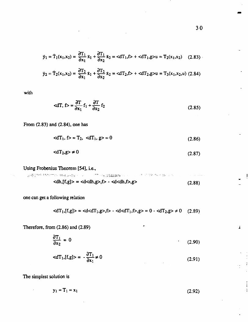
Yl = "lh(xl,x2) =
Y2= T2(xl,x2) =
_T1 aT1
_tl + _ _-2 = <dTt,f> + <dTl,g>u = T2(xI,x2) (2.83)
_T2 _T2
_Xl _1 + _22 Y_2= <dT2,f> + <dT2,g>u = T3(xl,x2,u) (2.84)
with
<dT, f> = _-_Xlfl + f2 (2.85)
From (2.83) and (2.84), one has
<dTl, f> = T2, <dTl, g> = 0 (2.86)
<dT2,g> _e 0 (2.87)
Using Frobenius Theorem [54], i.e.,
<dh,[f,g]> = <d<dh,g>,f> - <d<dh,f>,g> (2.88)v
one can get a following relation
<dTl,[f,g]> = <d<dTl,g>,f> - <d<dTl,f>,g> = 0 - <dT2,g> # 0 (2.89)
Therefore, from (2.86) and (2.89)
_T--k = 0Ox2
<dTl,[f,g]> = _TI #o
(2.90)
(2.91)
2
The simplest solution is
Yl = T1 Xl (2.92)

31
and from (2.86)
Y2 - T2 - <dT1,f> = x2 (2.93)
The feedback lincarization control u can be obtained from (2.84) as follows:
v - <dT2,f> v+G+Kx 2u = = = v + G + Kx_ (2.94)
<dT2,g> 1
Second, considerMcyer's approach. Sincethemotion issingledegreeof motion,
changecoordinateby setting
Y = x (2.95)
After differentiating until control term u appears, the system can be expressed as follows:
_'=_ (2.96)
_'=_12 =- G- Kx_ + u (2.97)
Define
Y = v (2.98)
The Bmnovsky controUerform is
with the feedback l.inearization control
u ---v + G + Kx_ (2. I00)

32
2.6°2.4 App|ieations
References 55, 56, and 57 designed an automatic flight controller for UH-1H
helicopter applying nonlinear transformation techniques and showed that the controller
exhibits good performance in all flight modes. As discussed in previous section, nonlinear
transformation technique based on Meyer approach needs to successively differentiate the
controlled states to get transformation map from nonlinear system to linear system. Meyer
presented a numerical approach for calculating these derivatives. A successive numerical
differentiation, however, requires formidable calculation, with attending numerical
difficulties.
To reduce the amount of computations, Menon [58] introduced singular perturbation
technique to simplify the nonlinear mapping for a flight test trajectory controller of high
performance airplane. The slow time scale controller follows path command and generates
steady state values for the body attitude. The fast time scale controller is designed to track
the commanded values for the body attitude. In Reference 18, the nonlinear
transformations have been used to derive pursuit-evasion guidance laws for high
performance aircraft.
Heiges [59] applied the above mentioned techniques to design a helicopter trajectory
controller and implemented it on the TMAN program. This controller has demonstrated
excellent performance in various tactical flight modes.
At
33
CHAPTER HI
TRAJECTORY PLANNING AS A ONE-SIDED
OPTIMAL CONTROL PROBLEM
3.1 Introduction
This chapter discusses the problem formulation and optimal trajectory synthesis using
two different performance indices. Candidate trajectories are generated and their optimality
is tested using second-variation analysis. Numerical effort involved in the computations
are analyzed.
For the f'u'st Optimal Route Planning problem, the terrain constraint is embedded into
state equations via a coordinate transformation. The performance index is a linear
combination of flight time and terrain altitude. In this problem, the computational algorithm
requires the fast and second partial derivatives of the terrain pxof'de.
The second Optimal Route Planning problem uses a performance index consisting of a
quadratic form in the terrain altitude, lateral deviation from the nominal trajectory, and
heading angle. By changing the independent variable from time to down-range, the order
of the problem is reduced. Each of these trajectory planning schemes will be discussed in
greater detail in the ensuing.

34
3.2 Optimal Route Plannin_ Problem No.!
3.2.1 Problem Formulation
A kinematic model of the helicopter will be employed in the ensuing analysis. Let the
terrain profile be specified by a function
ht = f (x,y) (3.1)
where ht is the altitude above a preselected datum at any specified position (x,y), x and y
being the down-range and cross-range measured in a chosen inertial frame. It is assumed
here that ht > 0 and that the terrain f(x,y) has continuous first and second partial
derivatives. This fact is important to ensure that the trajectories emerging from this optimal
trajectory planning problem are implementable. Additionally, this is consistent with the
proposed cubic spline parameterization of the digital terrain data. While executing nap-of-
the-earth flight, the helicopter altitude motion will follow the terrain profile (3.1) with a
specified altitude clearance. As a result, the helicopter altitude at any location (x,y) is given
by the equation
h - f (x,y) + he (3.2)
In (3.2), h is the helicopter altitude and 1_ is the specified terrain clearance. For NOE
flight, the clearance is between 5 and 120 feet [1].
A sample terrain profile with the x, y, h coordinate system is shown in Figure 3.1.
The local coordinate system x,, Ye, ze used in subsequent analysis is also defined in this
figure. This moving coordinate system has its origin on the terrain surface at the current x,
y position with x,-y, plane being the tangent plane. The principal direction of this system
is along the intersection of the x,-y e plane with the x-h plane. Accordingly, z, points in the
v

35
direction of the normal vector to the local tangent plane. The transformation of vectorial
quantities from one system to the other can be accomplished using the terrain gradients: see
Appendix A for details. Since the helicopter is constrained to move on the surface defined
by equation (3.2), the velocity vector lies in the instantaneous xt-yt plane, with the angle Z
defining its orientation on this plane. The helicopter velocity components in the local frame
can be resolved as:
Xe = V cos Z (3.3)
S't = V sin Z (3.4)
The local heading angle Z and the airspeed V are assumed to be the control variables in the
present trajectory planning problem
Note that it is important to include velocity as a control variable in the present problem
to ensure hodograph convexity required for the existence of optimal controls [60]. In order
to ensure that the control emerging from this formulation are implementable, the helicopter
speed is next bounded as
0 < Vmin <_.V < Vmax (3.5)
Because a simple kinematic system is considered here, Vm_ corresponds to the speed at
which sufficient excess power is available for avoiding unknown obstacles.
The velocity components (3.3) and (3.4) may next be transformed to the down-range,
cross-range, altitude frame using the relations
V cos Z V fxfy sin Z
X= _ ' ql+f_'q fzxf§r'-'-="--l+-- +- (3.6)
36
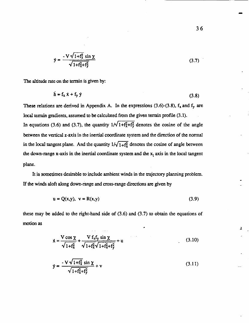
-v 14i7- sinZ3>= (3.7)
The altitu_ rate on the terrain is given by:
fi=f_x+fyY (3.8)
These relations are derived in Appendix A. In the expressions (3.6)-(3.8), fx and fy are
local terrain gradients, assumed to be calculated from the given terrain profile (3.1).
In equations (3.6) and (3.7), the quantity 1/_/1+_+_ denotes the cosine of the angle
between the vertical z-axis in the inertial coordinate system and the direction of the normal
in the local tangent plane. And the quantity 1/l'_f_+_x denotes the cosine of angle between
the down-range x-axis in the inertial coordinate system and the x I axis in the local tangent
plane.
It is sometimes desirable to include ambient winds in the trajectory planning problem.
ff the winds aloft along down-range and cross-range directions are given by
u = Q(x,y), v = R(x,y) (3.9)
these may be added to the right-hand side of (3.6) and (3.7) to obtain the equations of
motion as
V cos X V fxfy sin= __ + _-u (3.10)
lqt_+f2x 1,_-_+_x_/l+f2xx+f 2
-V l"v_+_xsinZ+v3>= (3.11)
41+_+_

37
The equations of motion (3.8), (3.10), (3.11) may be used whenever the helicopter is
flying in a terrain-following/terrain-avoidance mode.
Known threats and obstacles may be incorporated in the trajectory planning problem
by defining threat overlays of the form
Ah = P(x,y) (3.12)
and adding them to the basic terrain profile given by equation (3.1). The composite profile
may then be used to define the equations of motion (3.10) and (3.11). In that case, the
resulting trajectories will exhibit automatic threat and obstacle avoidance characteristics.
Additionally, it is possible to consider a formulation in which the specific energy of the
helicopter is maintained constant. This will occur whenever the throttle is set to maintain
thrust equal to drag while executing the nap-of-the-earth flight. In this case, the airspeed
will depend on the terrain profile as:
V = '/2g [E - fix,y) - 1%] (3.13)
In (3.13), g is the acceleration due to gravity and E = h + V2/2g is the specific energy.
3.2.20vtimal Route Planniw,F.
The performance index considered in this problem is a linear combination of flight time
and a terrain masking function. Following the existing literature [7], trajectory masking
will be assumed to be accomplished if an integral proportional to the helicopter altitude is
minimized. Admittedly, this masking function is crude since it is based on the contention
that depressed terrain tends to provide a better masking. If improved terrain masking
functions given as a function of down-range x and cross-range y were available, they can
be included in the following analysis without difficulty. For simplicity, in all that follows,

38
the terrain masking will be assumed to be accomplished if the integral of helicopter altitude
is minimized. A relative weighting factor is next introduced between the flight time and the
terrain masking function to control the trade-off between these two, often conflicting
requirements. Thus, a composite performance index of the form
J ---f [ (I-K) + K f (x,y) ] dt (3.14)
0
with
0<K_< 1 (3.15)
will be used in the following.
The initial conditions
x(to) = x0, Y(to)= Y0: given (3.16)
and the temainal conditions
x(tf) = xf, y(tf) = yf: given (3.17)
The variational Hamiltonian [12] may next be formed.by adjoining the differential
constraints (3.6), (3.7) to the performance index (3.14) to yield:: :
H 1 K+Kf(x,y)+Xx(VC°s_ .V fxfysin_g
= . _- _____ _ )_/i+_/1+_+_
+ _ (- V 1_+-_ sin Z) (3.18)
Note that the wind components have been dropped from (3.18).

39
where
The Euler-Lagrange equations for this optimal control problem arc:
_,y= -Kfy
B1 sin X X7 + (B2 sin g + B3 cos Z) _,x V3 3
AIA2
B4 sin X _ + (B5 sin X + B6 cos X) _.x V3 3
A1A2
A_ =_+_
A:=41+q+
B 2 --- {fxfxx A2 + A2(fyfxy + fxfxx)}fxfy + A 2 A 2 (fxfxy + fyfxx)
B3 =- A_ fxfxx
B4 = {- A_ fxfxy + A 2 (fxfxy + fyfyy)} A_
B5 =- {fxfxyA_ + A_(fxfxy + fyf.)}fxfy + A] A_ (fyfxy + fxfyy)
B6 =- A_ fxfxy
withtheoptimality condition
_.xfxfy-_.y (I+_)
tan)c= gx41+_+fy2
(3.19)
(3.20)
(3.21)
The equations (3.6), (3.7), (3.19), and (3.20) together with (3.21) constitute a nonlinear
two point boundary value problem, which can be solved if the initial conditions on the two

40
costates_.xand _.y were known. However, since the variational Hamiltonian is not
explicitly dependent on time and the final time is free, this optimal control problem has a
constant of motion, viz.,
H(t) = 0, 0 < t < tf (3.22)
i.e.,
0 = 1 - K + K fix,y) + _,x (V cosz
(3.23)
This constant of motion may be employed to eliminate one of the costates in the
problem. Using (3.21) and (3.23), one may solve for the costates kx and 7ty as
{1- K + K f(x,y)} _ + _ cos (3.24)=- ZV
2ty - {1- K + K f(x,y) }(_/1 + fZx+ _ sin Z- fxf_ cos Z)v4i+
(3.25)
Additionally, the costates can be completely eliminated from this problem by employing an
adjoint-control transformation as illustrated in the following.
The expressions (3.24) and (3.25) are next differentiated with respect to time and
equated to the right hand sides of the equations (3.19) or (3.20). This process yields a
differential equation for Z as:
• {(A 1K +A2) cos Z +A3(A4K +A 5) sin Z} V
Z = A6(AvK + 1) (3.26)
41
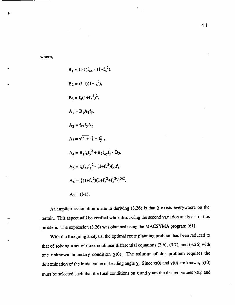
where,
B 1 = (f-1)fm - (l+fx2),
B2 = (l-f)(l+fx2),
B3 = fx(l+fx2) 2,
A l = BIA3_,
A 2 = fxxfyA 3,
A4 = Blfxfy 2 + a2fxyfy- a3,
A 5 = fxfxxfy 2 - (l+fx2)fxyfy,
A 6 = {(I+fx2)(l+fx2+fy2)}3/2,
A 7 = if-l).
An implicit assumption made in deriving (3.26) is that X exists everywhere on the
terrain. This aspect will be verified while discussing the second variation analysis for this
problem. The expression (3.26) was obtained using the MACSYMA program [61].
With the foregoing analysis, the optimal route planning problem has been reduced to
that of solving a set of three nonlinear differential equations (3.6), (3.7), and (3.26) with
one unknown boundary condition X(0). The solution of this problem requires the
determination of the initial value of heading angle X. Since x(0) and y(0) are known, X(0)
must be selected such that the final conditions on x and y are the desired values x(tf) and

42
y(tf). A simple iterative technique such as the method of bisections [62] may be set up to
solve this problem. Flow chart of such an iterative scheme is illustrated in Figure 3.2. If a
solution for the system (3.6), (3.7) and (3.26) satisfying the given boundary conditions
exists within the given _(0) range, then it can be shown that the scheme given in Figure 2
will find it in finite number of iterations [62]. Moreover, enforcing the conditions for the
existence of optimal controls can yield further guarantees on the convergence of this
numericalalgorithm.
Considernext,thesecondcontrolvariableinthisproblem,viz.,thehelicopterspeed.
SincethesecondcontrolvariableV appearslinearlyinthevariationalHarniltonianand is
bounded,theoptimalcontrolisgivenby
V = Vmax, ifS <0
V = Vm_,, ifS >0
V = Singular,S m 0 (3.27)
v
where S is the switching function obtained from
OHS_=_
OV (3.28)
namely,
S = _'x (_/1 + _ + _ c°s X + fxfY sin Z)" gY(1 + f'2_)sin x (3.29)
4T+q 41+_+_
2
=
:I
Substituting 2tx and gy from (3.23) and (3.24) into (3.29)
S _,..
{(I- K) + K f}
V (3.30)
43
Since V is always positive, the sign of the switch function is determined by the term within
the braces. This term is always less than zero by definition (0 < K _< 1, 0 < f). This
expression suggests that the maximum speed setting is optimal throughout the trajectory.
Euler solutions for the optimal trajectory planning problem may be generated by
numerically integrating the three fa'st order nonlinear differential equations (3.6), (3.7), and
(3.26). Starting from arbitrary initial conditions x(0) and y(0), Euler solutions to various
end conditions can be generated by changing the initial value of the heading angle. In the
present work, a sample terrain data from the U.S. Geological Survey [63] was used. The
terrain approximates a part of the Nassau Valley area in California shown in Figure 3.3.
The terrain data is stored at 1000 feet intervals and interpolated using Cubic Spline Lattices
[64]. This terrain data is given in Table 3.1. First and second gradients of the terrain
profile required in subsequent calculations are generated by differentiating the spline
polynominals analytically and substituting for down-range and cross-range values. The
nonlinear differential equations are integrated using a fixed-step fifth-order Runge-Kutta-
Merson technique and the method of bisections is used to carry out the one-dimensional
search. All computations were carried out on a VAX 11/750 computer system with double
precision arithmetic.
Figure 3.4 illustrates time-optimal trajectories starting at the point O and terminating at
several end points. These trajectories were obtained by setting K= 0 and varying the initial
value of the heading angle. This value of K corresponds to the case of time-optimal
control. The trajectories appear to be close to straight lines except in regions of large terrain
curvature. A family of Euler solutions starting at the point O with a large weight on the
terrain masking (K = 0.99) is given in Figure 3.5. These trajectories exhibit a more
significant curvature. An interesting feature of this solution family is that some of the
trajectories appear to intersect in certain regions of the given terrain. This implies the

44
existence of more than one trajectory satisfying the stationary and boundary conditions. In
this situation, the selection of a particular path has to be based on second order necessary
conditions. Such an analysis will be presented in the Section 3.4. For a typical set of
boundary conditions, Figure 3.6 illustrates the difference between time optimal and
maximum terrain masking trajectories with initial heading angles 50 and 68 degrees,
respectively. It may be observedfrom this figure that the te_nmasking trajectory tends
to seek out lower elevations while time optimal trajectories appear to minimize the arc
length.
3.3 Ontimal Route Planning Problem No.2
In the trajectory planning scheme discussed in the foregoing, the computation of
extremals required first and second partial derivatives of the terrain profile. In some
situations, it may not be desirable to compute these derivatives due to the nature of terrain
data. A formulation of the trajectory problem that does not require these partial derivatives
will be discussed next.
3.3.1 Problem Formulation
,iw
Assuming that the helicopter has a speed of V, the flighi'path angle y and the heading
angle _, the velocity components in the defined inertial reference frame is given.by
_t = V cosy cos_ (3.31)
y = V cosy sin_ (3.32)
The heading angle is the control variable in the this problem, while the flight path angle is
defined by the terrain profile. This is due to the fact that the helicopter is executing terrain

45
following flight. Thus, the kinematic model of the helicopter flight is given by the
differential equations (3.31), (3.32) and a nonlinear algebraic equation (3.2). In addition to
this, one can define three differential equations describing the point mass dynamics of the
helicopter. While it is desirable to include this in the formulation, the resulting trajectory
optimization problem becomes intractable. Note that it is possible to correct the present
results for neglected dynamics using singular perturbation theory [65 - 67]. The present
research will not address this aspect of the optimal trajectory synthesis problem.
In the ensuing formulation, time is not included in the performance index. Moreover,
since time does not appear explicitly on the right-hand side of equations (3.31) and (3.32),
the independent variable is next changed from time to down-range. This yields a dynamic
equation of the form
y'= tan _ (3.33)
Here, a prime over the variables represents differentiation with respect to down-range, the
independent variable in this problem. Note that this formulation is independent of the
vehicle velocity V. As a consequence, it is possible to impose an additional acceleration
constraint on the problem. It needs to be underscored that the vehicle velocity cannot be
permitted to be zero along the trajectory. Otherwise, the present modelling will lose its
P
validity.
3.3.2 Optimal Trajectory Planning
Assuming that the nominal trajectory to be flown by the helicopter is given by the
function yc(x), the objective of the second trajectory planning scheme is to maximize terrain
masking while minimizing deviations from the nominal trajectory. With this point of view,
the equation (3.33) may be modified as:

46
By'= tan W -yc'(x) (3.34)
Here, y¢'(x)isthe derivativeof the command yc(x) with respect to down-range x. The
heading angle _ is the control variable in thisproblem. The second optimal control
problem isthendefined as:
X
1 ff + _Sy 2 + CxV'2) dx (3.35)rain -_ (f2¥(t) "X 0
subjecttothe differentialconstraint(3.34).The quantitiesE and a arc factorsthatcontrol
therelativeweight between deviationsfrom the specifiedpath and lateralacceleration.For
mathcmatic_l convenience' wc next replace the tcrrncorresponding to V 2 with tan2_.
Moreover, the nominal trajectoryisoftenspecifiedby straightlinesegments. In thiscase,
one can redefinethe originof the coordinate system atthe initialpoint with the abscissa
pointingin the directionof thedown-range directionwithout any lossof generality.In this
case,the quantity8y can be set equal to y.
With thesemodifications,the optimalcontrolproblem isredefinedas
X
miny, 1 j'x_(f2 + ¢y2+ ay,2)d x (3.36)
.P
The Eulcr'snecessaryconditionforthisproblem can be obtained [12]:
(Ey + fly)
cx (3.37)
Equation (3.37) is a nonlinear second order differential equation with a varying coefficient.
The initial condition y(x 0) and the final condition y(xf) are specified. As in the previous
section, the quantity fy is the gradient of the terrain profile in the cross-range direction. The
Eulcr's necessary conditions can be obtained via two distinct, although equivalent

47
approaches. First, one may use the classical calculus of variations to derive (3.37).
Alternative approach is to let y" = U and proceed via modern optimal control theory [12].
Here, U is the control variable.
Numerical solutions to the differential equation (3.37) yield the extremals. To
construct an extremal joining a pair of x,y boundary conditions, the unknown initial
condition y'(0) needs to be determined.
Since just one unknown parameter is involved, it is possible to employ the method of
bisections to find the solution. Moreover, linear interpolation may be employed for terrain
interpolation since the method outlined here requires just the fast gradient of the terrain
profile.
Figure 3.14 shows a typical set of Euler solutions starting at the point O for 0t = 105, E
= 0.001. These trajectories were generated by changing the initial value of y' and
integrating the Euler's necessary condition forward. Note that the effect of increasing ot is
to produce trajectories that are closer to straight lines, while the influence of increasing E is
to introduce more features into the solution.
Figure 3.15 illustrates two trajectories with same boundary conditions, one being a
straight line joining the initial and final points and another being the extremal generated by
integrating equation (3.37). This trajectory corresponds to ot = 106, E = 0.01, and initial
heading angle --- -45 deg. Nature of the extremal agrees with general intuition that
helicopter should fly at lower altitudes and its path may zigzag around hills. Altitude
profiles along two trajectories in Figure 3.16 further iUustrate this fact.

48
3.4 Second-Variation Analysis
It can be shown that a sufficient condition for the extremals obtained in the foregoing
to provide a weak local minimum for an oPtimal control problem is that the second variation
be strongly positive [68]. The second variation wiU be strongly positive if the Legendre-
Clebsch necessary condition is met in the strengthened form and the no-conjugate point test
is satisfied. In optimal control problems with unbounded controls, it can be shown that the
variational Hamihonian is equivalent to the Weicrstrass excess function [68]. As a result if
the second variation tests are satisfied, then the cxtremals provide a strong local minimum.
In addition to this, it is known [69] that if the integrand of the performance index satisfies a
convexity condition, the extremals affording strong local minimum also provide a global
minimum. In the following, each of these conditions will be examined for the two
previous problems.
3.4.1 Second-Variation Analysis for O.R.P. #1
3.4.1.1 Le_endre-Clebsch Necessary Conditionv
In an earlier section, it was shown that the optimal value of airspeed V = Vmax. Since
this control variable appears linearly in the Hamiltonian, the.Lcgendre-Clebsch condition
reduces to the scalar form
Hzz > 0 (3.38)
Taking second partial derivative of the Hamihonian (3.18) with respect to control Z,
- kx (41 + _ + _ cosx + fxfy sinz) + L¢(1 + f2x)sinz V (3.39)
HXZ= "V_+_ _/I +_+_
w
I
49
Next, substituting kx and 2_y from (3.24) and (3.25) into (3.39), one obtains
Hxz = (l-K)+ K f(x,y) (3.40)
The fight-hand side of (3.40) is strictly positive by definition. Thus, the Legendre-
Clebsch condition is satisfied in the strengthened form at every point on the terrain. The
implication of this is that the problem is regular. As a result, the extremals will be smooth
and provide a weak local minimum for sufficiently short intervals.
3.4.1.2 Wgierstrass Test
In the Calculus of Variations, strong variations only bound the magnitude of 5x, while
weak variations bound both the magnitude of 8x and the magnitude of the time derivative of
8x [35]. Weierstrass gave a test for verifying strong local minimum characteristics of
extremals. It can be shown that the Weierstrass's excess function [68] is equivalent to the
Variational Hamiltonian in optimal control theory [12].
• ,,. ..... ,.., cosx fxfysinz }-k V "*''xsinZH(x,_.,_,t) = l-h+ra+A.xVt -I
Substituting _.x and ky from (3.24) and (3.25) into (3.41), one has
H(x,_.,X,0= (I-K + K f)[I-cos (X° -X)}
Here, _o is the value of Z satisfying the optimal condition I-Iz--0.
and
(3.41)
(3.42)
H(x,_.,Z,t) > H(x,k,Z°,t) = 0 (3.43)

5O
In the foregoing it has been shown that the Weierstrass necessary condition is satisfied
along the extremal. Thus, the performance along the extremal is lower than along any other
trajectory.
3.4.1.3 Jacob| Test
For extremals of finite length, the task of ensuring that the=second variation is
nonnegative for admissible variations leads to the accessory-minimum problem in the
calculus of variations. This problem attempts to produce a system of admissible variations,
not identically zero, which offer the most severe competition in the sense of minimizing the
second variation. If a system of nonzero variations making the second variation zero can
be found, then a neighboring trajectory is competitive. In this case, Me test extremal
furnishes at best an improper minimum and at worst a merely stationary value [70]. First
value of the independent variable for which such a nontrivial system of variations can be
found defines a conjugate-point.
It has been shown in the references [i2][71][72] that the accessory _nimum problem
leads to the analysis of the nature of solutions to lincarized Euler-Lagrange equations. We
note here that this problem may be cast in the standard linear-quadratic format using the
backward sweep method [12]. However, algebraic linearization of the Euler-Lagrangc
equations (3.6), (3.7), (3.19), (3.20) can become excessively'involved. As an alternative,
a numerical conjugate point test will be employed in the present research. Reference 73
discusses several numerical methods available for conjugate-point testing. A direct
approach for conjugate point testing will be pursued in the following. This approach is
based on Theorem 12.1 -12.3 in Reference 70. This theorem is discussed in detail in
w --
Appendix B.

5I
From the existanc¢ theory of linear ordinary differential equations [74], it is known
that the solutions to the linearized Euler-Lagrange equations should be linearly independent.
More concisely, the Wronskian determinant should not be zero on an open interval. For
these fundamental solutions to be unique, they should be nontrivial and satisfy initial
conditions.
In the present problem, the fundamental solutions axe obtained by using the finite-
difference approximation
8xl (t) = x'(t) - xi(t),
dx2 (t) = x'(t) - xi(0,
8yl (t) = y*(t) - yi(t)
dy2 (0 = y*(t) - yJCt)(3.44)
where (xi(0,yi(t)) and (xJ(t),yJ(t)) are neighboring extremals generated by perturbing the
initial value of heading angle. Note that this is equivalent to perturbing the initial value of
costates, while maintaining the appropriate state initial conditions.
The characteristic determinant A(0 is then formed as:
A(t) -] 8Xl(t) 8x2(t) ] (3.45)8yl(t) 8y2(t)
From the theory of differential equations [74] it is known that this determinant cannot ber
identically zero. If this characteristic determinant (3.45) after being zero at initial t = 0,
subsequently becomes zero at t = t*, with t* < tf, then the point t* is said to be conjugate to
the initial point t = 0.
This numerical conjugate point test is applied to the maximum masking extremals
given in Figure 3.5 with K--0.99. In this figure, the extremals A and B are of particular
interest since these are competing extremals satisfying the boundary condition pair (O, F).
The characteristic determinant (3.45) evaluated along these extremals is given in Figures

52
3.8 and 3.9. From these figures it is clear that a conjugate point to point O occurs along the
extremal B, while none is encountered along extremal A. Thus, the extremal A affords a
strong local minimum if the desired end conditions were points O and F. On the other
hand, the extremal B provides merely a stationary value. This fact is confirmed by
computing the performance index along these trajectories and given in Figure 3.10. This
figure indirectly proves the princple of optimality by showing that the performance index
along optimal trajectory A between two points O and F is always lower than neithboring
extremal B. The point conjugate to the point O along extremal B is denoted by the point C
in Figure 3.5. A rule of thumb given in Reference 75 is that a conjugate point can be
expected to exist at point where the tangent to the extremal experiences a sudden change.
In the present case, it may be observed that the extremaI B experiences a sharp turn at the
point C.
In the minimum flight time problem' K = 0, the integrand of the performance index is
a constant, and it does satisfy the weak convex condition given in Reference 69. Thus the
extremals satisfying three second variation tests also provide a global optimum [69].
In Figure 3.11, two extremals satisfying the boundary condition pair (O, F) are given
for the rain-time criterion. Following the same procedure as for the maximum masking
problem, the characteristic determinant evaluated along these extremals is given in Figures
3.12 and 3.13. From these figures it is clear that a conjugate'point to point O occurs along
the extremal A, while none is encountered along extremal B. Thus, the extremal B affords
a global minimum if the desired end conditions were points O and F. On the other hand,
the extremal A provides merely a stationary value.
../,

53
3.4.2 Second-Variation Analysis for O.R.P. #2
For the second trajectory planning problem, the Legendre-Clebsch condition will be
met in strengthened form ff ¢x> 0, since the Legendre-Clebsch necessary condition [76] is
_-_22 2]fff2 + _Sy 2 + a_g 2) = a > 0 (3.46)
Defining F(x,y,y') = f2 + ey2 + ay,2, the Weierstrass excess function for this problem
turns out to be
E (x,y,y',p) - F(x,y,y') - F(x,y,p) - (y'-p)Fp(x,y,p) = ¢x (y,.p)2 (3.47)
This is positive if y' is not equal to p.
The Jacobi's differential equation [76] for this problem turns out to be:
vi" =_ (E + t'Zy+ f fry) n (3.48)
Here aq is the solution to the linearized Euler-Lagrange equations or the second-variation. If
the coefficient 1 (E + _ + f fry) on the fight hand side is a slowly varying quantity with
respect to range, additional analytic results may be obtained using the WKB method [16].
Let
q(x) = _ (e + _ + f fry) (3.49)
where x is the stretched range x = I.t x, t.t > 0. Equation (3.48) can be rewritten
_" - q(x) T! = 0 (3.50)
The various derivatives in the above differential equation can now be written as

54
dn dndx=
withchange ofvariableIx= _.-I
. _.2q(x)Tl= 0
(3.51)
(3.52)
(3.53)
(3.54)
The equation (3.54) with a large parameter X is referred to as Liouville's problem [74]. Its
approximate solution can be obtained using WKB method [16].
xf xf _A'_
11 = q-_C1 cos (JXo w/q'dx)+C2sin (fxo-v_dx)}, when
xf xf
(3.55)
(3.56)
T
z
where C1, (22 are arbitrary constants. It may be observed from the above solutions that if
q > 0 in the given interval, there are no conjugate points. Since f > 0 by definition, this
expression implies that q is always positive if fyy > 0. That is, if the vehicle is traveling in
a valley or along a saddle, the resulting extremal will not contain any conjugate points.
In the cases where q(x) changes sign along a given extremal, one has to carry out this
test numerically. The procedure employed in the previous trajectory planning technique
may once again be used. It may be verified that the integrand of the performance index

55
satisfies the convexity condition given in [69]. As a result, ff a given extremal satisfies the
second order necessary conditions, it affords a global minimum.
3.5 Comnutational Effort
3.$.1 Comvutational Effort for O.R.P. #1
Studies using a VAX 11/750 computer have shown that an extremal requiring about 70
integration steps consumes between 1.5-2.1 seconds of CPU time. Given the desired
initial and f'mal conditions on down-range and cross-range, several Euler solutions need to
be evaluated to converge on the one satisfying the given boundary conditions. Using the
computational flow chart in Figure 3.2, between six and seven iterations were found
adequate to reduce the boundary condition error by an order of magnitude. Clearly, this
will depend on the given terrain profile. For example, ff the terrain gradients fx and fy were
small such that the boundary condition error depends approximately linearly on the initial
heading angle error, the number of iterations and boundary condition error may be related
as using the convergence formula for the method of bisections [62] as:
r = In (%/%,) (3.57)In 2
In the expression (3.57), r is the number of iterations, ey 1is the initial boundary condition
error and %ris the boundary condition error after r iterations. It is important to stress here
that this relationship does not account for nonlinearities due to terrain profile. Its
usefulness is limited to generating a first order estimate on the number of iterations required
to satisfy a specified boundary condition error tolerance.

56
In the present research the total computations for one step integration are about 626
multiplications and divisions and 240 additions and substractions.
3.5.2 Comnutational Effort for O.R.P. #2
Assuming that the stationary condition (3.37) is integrated using the Euler's method,
and that a linear interpolation is employed for computing the terrain altitude at various
down-range and cross-range locations, one can obtain a formula for the required number of
operations. In the following, it is assumed that multiplication, division, addition, and
subtraction each count as one operation. Each integration step is found to require 23
operations. The method of bisections requires two mathematical operations and one logical
operation per iteration. Thus, if there are n discretization intervals in the down-range
_tion and r bisections iterations, the _seni:_thbd would req_ approximately
m = 23 nr (3.58)
operations. Assuming that it is desired to decrease the interval of uncertainty by two orders
of magnitude, one requires about 7 iterations using the method of bisections. Thus, the
number of operations required for the method of bisections is m = 161n. Note that one can
reduce the interval of uncertainty by eight orders of magnitude by increasing the number of
iterations by about four times.
Next, assuming equal discretization of the down-range and cross-range directions, the
dynamic programming scheme is found to require 23 mathematical operations per node to
evaluate the performance index. In a typical computing scheme [12], this will have to be
evaluated at n 2- 1 nodes. After these computations, one has to execute 2n -1 logical

57
operations. Thus, the total number of operations required in a full scale discrete dynamic
programming approach for the present route planning problem is approximately
m = 23 n 2 + 2n (3.59)
operations. Thus, to first order, the two methods are equal in terms of computational speed
whenever n = 7. Whenever the number of discretization intervals exceeds this figure, the
present approach provides a faster solution. In any case, note that the computational effort
in the present approach is a linear function of the number of discretization interval, while in
the dynamic programming approach, the computational effort is quadratic in the number of
discretization intervals.
On a rough terrain, one would require a large number of discretization intervals to
obtain results with sufficient fidelity. In that situation, the advantage of the present
approach will be even more significant. On the other hand, the dynamic programming
approach guarantees the optimality of the solution, while in the Euler solution method, this
has to be verified through second order necessary conditions.
3.6 Wind Effects
The magnitude and direction of winds are known to have a substantial effect on the
performance of most aircraft. This effect is accentuated on a conventiona_ helicopter
because of the low flight speeds, As mentioned in Section 3.2, the ambient winds can be
incorporated into the trajectory programming scheme with slight increase in complexity.
For the purposes of illustration, the effect of constant winds along x-axis in the first
trajectory planning problem will be considered. Using equations (3.8), (3.10), and (3.11),
and assuming the same performance index (3.14), one can obtain costate equations as

58
- {1 - K + K f(x,y)} "_ + _ cos Z_.x = (3.60)
v +u4/+ _ cosz
_.y= {1- K + K f!x,y)}(_/1 + _ + _ sin Z- fxfy cos Z) (3.61)4/+ c¢+u4"/+ cosz)
Following the same steps as in Subsection 3.3.1, the differential equation for heading
angle _ turns out to be
= V (C1 sin X + C2 cos X) + u A1 cos Z (D1 sin Z + D2 cos Z) (3.62)(I-K+Kf)A A
where,
A2=_/l+_+_
B I= {-A_ fxfxx+ A21(fyfxy+ fxfxx)}A1
v
B2 "- {fxfxxA2 + A21(fyfxy+ fxfxx)}fxfy+ A21A 2 (fxfxy+ fyfxx)
CI =- KfxA_ A_-(I- K + Kf) BIA2
C2 =- KfyA21A_ + (I- K + Kf) {B1fxfy+ B2 + A_fxfxx(fxfy-f.xyA2)}
M.
D: =- KfxA21A32+ (I- K + Kf) (- BIA2 + A_fxfxx)
2 3D2 = - KA1A2 (1 + fy)2 + (1 - K + Kf) (Blfxfy + B2)
The accuracyof theseexpressionsmay bc verifiedby puttingthewind spccdu tozero.
In thiscase,the equation(3.62)exactlycorrespondsto (3.26).Figures3.17 and 3.18

59
show several extremals for the minimum flight criterion and the maximum masking
criterion when wind to airspeed ratio u/V equals to 0.1 and all conditions being the same as
the Figures 3.4 and 3.5. An observation that may be made from these figures is that the
winds affect the maximum masking trajectory to a higher degree.
It is possible to include wind effects in the second route planning problem also.
However, this will not be pursued in the present research.
3.7 Conclusion
In this chapter, two systematic methodologies for optimal trajectory planning (ORP)
useful in the helicopter terrain-following/terrain-avoidance flight was presented.
For the ORP No.i, the terrain constraint was embedded into state equations via a
coordinate transformation. The performance index consisted of a linear combination of
flight time and terrain masking. Using an adjoint-control transformation, the optimal
control problem solution was reduced to a search for the initial value of heading angle. It
was shown that the optimal airspeed, a second control variable in the formulation, should
be chosen as the maximum permissible value. A simple computational scheme based on
the method of bisections and a fifth order Kutta-Merson numerical integration technique
was outlined for generating Euler solutions. Families of I_uler solutions for minimum
flight time and maximum terrain masking were presented.
It was shown that the Legendre-Clebsch necessary condition and Weierstrass excess
function are satisfied everywhere in the admissible region. Further, conjugate points have
been shown to occur in certain regions of the specified terrain. In the regions where
conjugate points do not occur, the Euler solutions for the maximum masking problem
provide a strong local minimum. The Euler solutions for the minimum time problem

6O
satisfying the second-order necessary conditions were shown to provide a global
minimum.
For the ORP No.2, the performance index consisted of a quadratic form in the terrain
altitude, lateral deviation from the nominal trajectory, and heading angle. By changing the
independent variable from time to down-range, the order of the problem was reduced.
The Legendre-Clebsch necessary condition and Weierstrass excess function were
satisfied everywhere in the admissible region. For this problem, an approximate conjugate
point test was developed using the WKB method.
The winds effects on the trajectories were briefly examined for ORP No. 1. It is found
that the winds affect the terrain masking trajectory to a higher degree.
l

61
CHAPTER IV
TRAJECTORY PLANNING AS A TWO-SIDED
OPTIMAL CONTROL PROBLEM
4.1 Introdu_tiQn
Previous chapter dealt with the situation wherein we seek to determine the optimal
trajectory for a vehicle to fly from an initial position to a given final position. In this
chapter we will examine the same problem involving two vehicles with conflicting
objectives.
In such a situation, the trajectory planning problem will turn out to be a differential
game. An example is the case where one of the vehicles is attempting to intercept the other
while flying in a terrain following mode to avoid detection. Meanwhile, the second vehicle
may be executing a terrain following flight with the objective of avoiding capture.
Problems of this nature have received scant attention in the previous literature [77].
Next generation military helicopters such as the LHX must have capabilities to
automatically engage with ground and air targets. The avionics requirements'for the low
altitude air combat mission are complex, and reflect the problems brought about by
simultaneous air combat and terrain flight [78].
Since the publication of Isaac's famous book [17], the homicidal chauffeur problem
has became a model for vehicle pursuit-evasion. The solutions to this problem are very
intricate and have been discussed in References 79 and 80. Ciletti [77] indicated that the
62
m
assumption of perfect information and role ambiguity [81] are some of the factors that have
prevented the application of differential games theory in realistic military situations.
Additionally, dynamics of the vehicles are highly nonlinear and of high order. These
factors have led to a situation wherein complete results are given only for a very limited
class of problems.
In this chapter, two different approaches are proposed for studying the helicopter
pursuit-evasion problem. A nonlinear pursuit-evasion game employing helicopter model
incorporating the terrain profile is discussed first. This model was used in Chapter III for
trajectory planning. This is followed by an approach based on the feedback linearization
technique motivated by the research in Reference 91. Each of these approaches will be
discussed in the following sections. In the ensuing, it will be assumed that each player has
complete information on the helicopter parameters and a noise free measurement of all the
state variables.
4,2 A Nonlinear Pursuit-Evasion Game
4.2.1 Problem Formulation
The helicopter pursuit-evasion problem is analyzed here _ a deterministic two-person
zero-sum differential game. The game begins at a certain set of initial conditions, when the
helicopters ftrst become aware of each other. In the present analysis the respective roles of
the players are assignedat the outset. It is assumed that this role definition remains
unchanged during the entire game. Although this formalism restricts the applicability of the
results, it is useful in revealing salient solution features. In real situations, the evader may
be a helicopter without offensive capabilities or with limited maneuvering capabilities.

63
4.2.1.1 Eouations of Motion
When compared with high performance aircraft pursuit-evasion, one of the
characteristics of helicopter pursuit-evasion [82, 83] is that each participant attempts to
reduce its exposure to the opponent by avoiding high altitude flight throughout the
engagement. This is due to the fact that the vertical maneuvering above NOE altitudes may
make the helicopters more vulnerable to detection by ground and air based surveillance
system. The equations of motion developed in Chapter HI are used here to model the
helicopter flight in terrain-following mode. In the interest of clarity, these equations of
motion are repeated here.
v, f,,.fy.sin_ Ve cos _ + (4.1)
1,_-'f2_ 1_-_/1 +f2_+f_.
Ve l_ sin 7_
S'e =" _/i+f_ +_. (4.2)
;tp = VP cos Zp +Vp fx,fy, sin Zp
14i;- ,41(4.3)
Vp l_xp sin Zp
YP = _/1 +_p+_y, (4.4)
The subscript e denotes the evader, while the subscript p denotes the pursuer. To make the
problem meaningful, it is assumed that the pursuer has a higher speed than the evader, i.e.,
Vp > Ve (4.5)

64
Wheneverthe terrain gradients fx, fy are zero, it is possible to show that the condition (4.5)
is essential to guarantee capture. The initial conditions at t = 0 are
(x_,ye)ltffio specified
(Xp,yp)It__-0 specified
(4.6)
(4.7)
This problem is a terrain following version of simple motion illustrated graphically in
Reference 17. The participants select the direction of travel and may change it as fast as
desired. Thus, the control variables in this problem are the heading angles, gp and ge.
Note that this pursuit-evasion game has a very simple solution whenever the terrain
gradients are zero. However, the solution becomes quite complex in the general case; as
will be apparent in the ensuing.
4.2.1.2 Termination of Game
The game terminates at the first instant the pursuer succeeds in approaching the evader
within the fu-ing range of its weapon system. For the case of a circular weapon range
envelope, this condition can be expressed by the requiring that
(xe - Xp) 2 + (Ye- yp)2 ] tt S d2 ,. (4.8a)
d {(Xe- Xp) 2 + (Ye- yp)2} < Odt (4.8b)
The quantity d is a specified number. The condition (4.8b) is required to ensure sufficient
time for weapon usage. The time of capture is determined from the requirement that
tf= rain {(Xe-Xp)2+(ye-yp )2-d2=0} (4.9)t
w

65
i.e., the instance that the condition (4.8a) is met as an equality.
It has been suggested in the literature [17] [84] that a fan-shaped capture set may be
more realistic. However, in all that follows, a circular envelope will only be considered.
4.2.1.3 Measure of Effectiveness
In the most planar games reported in the literature [80] [85], the performance index of
the game is the time of capture. The objective of the pursuer is to minimize the terminal
time tf, while the evader endeavors to maximize it. Additionally, in the present setting both
players also attempt to minimize their flight altitude to ensure adequate terrain masking. In
this case, the performance index can be expressed as
tf
J = rain max _(1+ W,f,-W,f.)& (4.10)Zp Z_ t
I
where, Wp and We are weighting factors for the pursuer's altitude and evader's altitude,
respectively. The negative sign on the second term explicitly recognizes the fact that the
evader is attempting to maximize the performance index. In order to satisfy the terminal
constraint (4.8), it may be appended to the performance index in the form of a penalty
function [12]. In this case, the augmented performance indexis
tf
ja= min max Q(tf)+ _(l+Wpfp-Wefe) dt (4.11)Z_ X, t
0
The terminal penalty function is given by
Q(tf) =_ {(xp- re) 2 + (yp- ye) 2- d2} It, (4.12)
and v is an undetermined multiplier in the game.

am.
66
4.2.2 Derivation_f Optimal Strategies
For convenience, define
rl--- Re, r2 -_ _'e, 1"3- _p, r4 --- yp (4.13)
The variational Hamiltonian [12] may be formulated as
4
H = 1+ Wp fp- We ire + X _,iri (4.14)i=l
Expression (4.14) may be written in a more succinct form as:
H = 1 + H(Xp) + H(ZD (4.15)
with
H(Xp) = Wp fp + _,3 1"3 + _4 r4
H(Ze) " - We fe + Xl rl + X21"2
(4.16)
(4.17)
Since H is separable in terms of pursuer-evader controls gp and Xe, the saddle point
condition [39] is satisfied. As a result, the order of maximization and minimization doesr
not influence the outcome of the game. Thus, one has
min max H= max min H• , z. z. t, (4.18)
The integrand of performance index (4.10) and system equations (4.1 - 4.4) are continuous
and satisfy the Lipschitz condition. Thus, the sufficient condition for the game to have the
value is also satisfied, see Appendix C for more details. Each player's goal is to reach the
value, i.e., saddle point of the performance index.

67
where
Euler-Lagrange equations for the evader are given by
_,1 = Wefxe "BI sin Ze k2 + (B2 sin Ze + B3 cos Ze) _-I Ve
3 3AIA2
_.2 = Wefye B4 sin Z_ _.2 + (B5 sin Ze + B6 COS Ze) _,I We3 3
AIA2
B2 =- {fxefxexeA_ + A21(fyefxee + fxefxexe) } fxefye
B3=- A_f_of_o
B, = {-A_f_/_y°+A_(f_of_o_°+f_.fyo_0)}A_
B5=- {f,_f_y_A_+ A_(f_of_yo+ fy0fyoy_)}f_;fyo
+A_A_(f_/_.o+f,.fyo_)
The Euler-Lagrange equations for the pursuer can be obtained as
DI sin Zp _L4 + (1)2 sin Zp + D3 cos Zp) _-3
_.3=- wpf_p- _c_Wp
(4.19)
(4.20)
(4.21)

68
= - W_yp D4 sin Zp 7,4 + (D5 sin ZV + D6 cos Zp) 2,3 Vp(4.22)
C_-- _/1+ _p
D1 -- {- C22fxpfxpxp + C_1 (fypfxpyp + fxpfxpxp)} C2
D2---{fxpfXpXpC_2 + _ll(fypfxpyp + fxpfXpxp)}fxpfyp
+ C_1 C_ (fxpfxpyp + fypfxpxp) : :
D 3 --- C_2 fxpfxpXp
D4 - [-_2 fxpfXpyp + C_I (fxpfxpyp + fypfypyp)} C_I
D 5 --- {fxpfXpypC 2 4-C_l(fxpfxpy p + fypfypyp)} fxpfyp
+ C_l C_ (fypfxpyp + fxpfypyp)
D6 =- _2 fxpfxpyp
The optimality conditions for the two participants are given by-
tanZ, = X_f_dY*"X2(1 + f2)2"1 _/1 +f2xe +_e
(4.23)
tan Xp = J_3fxvfYp - X4 (1 + _p)
_'3 41 +f2Xp +i¢2yp(4.24)
Terminal conditions on costates can be obtained from the terminal penalty function as
69
_.l(tf) - _ - - V(Xp-Xe)
____.2(tf) - _ - - V(yp-ye)
V(Xp-X )_,3(tf) = o_x"_" =
D
;L4(tf) = _- v(yp-y=)
(4.25).
(4.26)
(4.27)
(4.28)
o-_ = 0 (4.29)H(tf) =- o_t---_-
Since the f'mal time tf is unspecified and the Hamiltonian does not explicitly depend on t,
this problem has a constant of motion, viz.,
H(t) = 0,0 _<t _; tr (4.30)
Substituting equations (4.25) - (4.28) into (4.14) and invoking (4.29), it is possible to
obtain an expression for the undetermined multiplier v as:
V _ 1+ Wp fp- W= fe It=tf(xv-xe)rl+(yp-ye)r2-(Xp-Xe)r3-(Yp-ye)r4
(4.31)
It may be verified that the denominator of equation (4.31) is simply the negative of the
product of range and range rate. Since the final value of the range is positive and the
terminal range rate is negative, the parameter v has a positive sign for the pure pursuit-
evasion game in which Wp = We -- 0. Moreover, expression (4.31) implies that at the final
time, if one requires the pursuer and evader's positions to match exactly, v would become
in/mite.

m
7O
4.2.3 Numerical Results
Most differential game solutions reported in the literature are obtained using numerical
methods. Among them, simple shooting in retrogressive time [86] [87], differential
dynamic programming [88], and gradient method [89] have been widely used. In certain
situations, the solutions obtained using reduced order modeling can be corrected for
neglected dynamics using singular perturbation techniques [90].
In the present research, retrogressive time integration is used to generate the extremals.
The trajectories are generated by first selecting the terminal position of the evader. The
terminal position of the pursuer is then selected from the specified capture set. This
corresponds to the expression (4.8a) being met as an equality. Substituting the final
costates into the optimality conditions (4.23) and (4.24) and noting that the unspecified
multiplier v exists in both numerator and denominator of these equations, the final values of
p_uer and evader*s_heading angle can be ca]cuiated. _e final values of rl, r2, r3, and r4
can be computed. Substituting these in equation (4.31) yields the unspecified multiplier v.
This enables the evaluation of the final value of the costates. The state-costate system is
then integrated backwards in time to obtain the pusuer-evader trajectories.
Figure 4.1 shows the pursuer and evader trajectories with terrain masking weights set
to zero. As in the one-sided trajectory optimization proble_n, the trajectories are nearly
straight lines. In Figure 4.2, the pursuit-evasion trajectories with Wp - 1,.We = 1 are
illustrated. The value of the parameter v is computed as v = 5.79E-3. With nonzero Wp
and We, the trajectories exhibit significant terrain masking features. Figure 4.3 illustrates
the altitude evolution as a function of time-to-go. Note that tgo = 0 corresponds to the game
termination instant. Pursuit-evasion trajectories for another set of initial and final
conditions with Wp = 1, We = 1 are given in Figure 4.4. The value of the parameter v is

71
computed in this case as v = 2.03E-3. The corresponding altitude history is given in
Figure 4.5. Figure 4.6 illustrates trajectories for the pursuer and evader with Wp = 0.0,
We = 1.0. Note that in this case, the pursuer does not attempt any terrain masking. As a
result, its trajectory is nearly a straight line joining the initial and final conditions. The
value of the parameter v is computed as v = -.747E-3. For Wp = 0.5 and We = 1.0, Figure
4.7 shows the pursuit-evasion trajectories with v = -.375E-3. For the same weighting W,,
the trajectories become more curved as the weighting Wp is increased.
Le_,endre-Clebsch Condition
The optimality conditions (4.23-4.24) do not guarantee that the players maximize or
minimize the performance index according to their role. To determine the correct optimal
controls that make the pursuer minimize the performance index, while making the evader
maximize, the verification of Legendre-Clebsch condition is necessary.
For the present differential game, the Legendre-Clebsch condition requires that
Hx, x.. < 0 (4.32)
Hx,,_ > 0 (4.33)
where ,p,
- kl 41 + f'2xe+ _ cos Z_ + {k2 (1 + f2xe)- _,lfxcf_e) sin Ze Ve
41+ 41+fL+ o
- _.3 "_ 1 + _p + _p cos gp + {_L4 (1 + _p)- _,3fxpfyp} sin %p
41+ p 41+ p+ p
(4.34)
Vp (4.35)
The conditions (4.32),(4.33) may be strengthened by requiring strict inequality.

72
Since these expressions are too difficult for hand computations, they are numerically
evaluated along the extrcmals. Figure 4.8 shows these quantities evaluated along the
trajectories in Figure 4.2. It may be seen that the Lcgendre-Clebsch necessary conditions
are satisfied in the strengthened form. Figure 4.9 illustrates the L-C test along the
extrcmals in Figure 4.4. In this c_, !tappcars that this test is satisfied in the strengthened= ............. =_.... _ ::: :_ _:_: ..........
form every whereexcept a smaU region near the final region. It is important to emphasize
that the Jacobi test needs to be carried out along these trajectories before concluding the
optimality. This will not be pursued any further in this thesis.
4.3 Feedback Linearized Solution to a Pursuit-Evasion Game
As illustrated in the previous section,the numerical solution of even simple differential
games requires a tremendous amount of computational effort. An approach proposed
recently for solving a class of differential games [18] is to transform a nonlinear model into
linear timc-invariant form. A linear differential game is then solved and the results arc
transformed back to original coordinates to obtain a nonlinear feedback law suitable for real
time implementation. The advantage of this approach is that it can handle high-order
nonlinear vehicle models in th_ analysis. In the following, such a differential game will be
formulated and solved. The ensuing formulation will employ a high order m.odel of the
helicopter,
2,
4.3.1 Vehicle Model
The point-mass model for a high performance helicopter can be expressed by the following
nonlinear differential equations:

73
= V cosy cos (4.36) "
y = V cosy sin (4.37)
fi=Vsin y
V = T sin 0m - g sin y
i
_/= g (T COSmgOcos
_t = T cos 0 sin ¢mV cos y
- COS '_)
(4.38)
(4.39)
(4.40)
(4.41)
Here, x is the down-range, y the cross-range, h altitude, V the speed, y the flight path
angle, V the heading angle, T the main rotor thrust, m the vehicle mass and g is the
acceleration due to gravity. Figure 4.10 shows the definition of the axis system. The
control variables are the pitch attitude of the helicopter 0, roll attitude of the helicopter _,
and the main rotor thrust T. If desired, one may model T in terms of two components.
The fhst depending only on the vehicle states To and the second component ST that
depends purely on the collective control, i.e., T = To + _iT. The assumptions involved in
this model are stationary atmosphere and uniform gravitational acceleration. It is important
to note that this highly simplified helicopter model does not permit hovering.
4.3.2 Problem Formulation
The point mass helicopter model (4.36) - (4.41) will be transformed to a linear, time-
invariant form in this section. Various steps involved in this transformation will be
discussed in detail.

74
In order to execute the terrain flight mode, admissible trajectories should satisfy the
terrain profile constraint, i.e., the vehicle altitude h should be:
h = hc + fix,y) (4.42)
This equality constraint can be absorbed into the state equations as witl be shown in the
foUowing. Differentiating the equation (4.42) with respect to time and noting that hc is a
constant, one has
fi = fx)t + fyy (4.43)
Equating (4.43) to (4.38), and substituting (4.36) and (4.37) for g and Y results in
tan 3'= fx cos ¥ + fy sin ¥ (4.44)
Differentiating once again with respect to time results in,
_t_t = fx_,_cosy + f_yycosy+fr_ sinv + f.y sinv- f, sinvff +fycosv_(4.45)
Next, substituting from (4.36), (4.37), (4.40), and (4.41) for_t,y,_/and_, and
rearranging yields the following relation
a-
T cos0 cos_ = mV2cos37 {(fxx cos_ + fxy sin_) COS_ + (fxy COS_ + fyy sin_) sin_}
+ (- fx sinv + fy cos V) cosy T cos0 sine + mg cosy (4.46)
The expression (4.46) relates the vehicle states and control variables to the terrain profile.
It specifies the vertical force required to ensure that the vehicle trajectory satisfies the
terrain profile constraint. As a result, this expression dictates the altitude dynamics for the
two vehicles.

75
Following Reference 18, the remaining components of the nonlinear helicopter models
for the pursuer and evader may be transformed into the Brunovsky canonical form by
differentiating the expressions (4.36) and (4.37) with respect to time and substituting for
X?, "_, V from the expressions (4.39) - (4.41). Defining four pseudo control variables, the
helicopter models can be put in the form
Rp =apl _p =_p2 (4.47)
= r_z Ye = _e2 (4.48)
where, _pI, _p2, _1 and _2 are the vehicle acceleration components in the earth-fixed
frame. These quantities may be related to the pursuer-evader states and controls as
_pl (Tp sin 0p Tp cos 0p sin _p sin Up= mp - g Sin 7p) COS 7p COS Up " mp
cosOp cosOp_ g (Tp mpg - cos Vp) sin _p COS Wp
(4.49)
sin 0pap2 -- (Tp mp
Tp cos Op sin _ cos Wp- g sin yp) cos 7p sin Wp + mp
T_ COS Op COS %. g (r . cos 7p) sin 7p sin Upmpg (4.50)
T sin 0_. Te c6s 0e sin _e sin_I = C e g sin%) cos 7e cos We -
Weme me
(% cos 0=cos $=-g meg -cos %) sin7e cos We
(4.51)
_.2 = _T_(._sin 0= _me g sin7e)cos % sinWe -t "recos ee sinSe cos Weme
f% cos e_ cos $=g meg - cos %) sin % sin We
(4.52)
R
76
Equations (4.47) and (4.48) are linear time-invariant form. If the pseudo control variables
_[pl, _[p2, gh:l and _.2 were known, the actual helicopter controls can be obtained using the
following equations:
_bp--tan"1(_p2cos_tp-aplsin_tp)Fp (4.53)
Op = tan-1 (S in _ Cap1 cos Vp + gp2 sin Vp +Fp sin yp) )('-ap2COS _p- _lpl sin _/p) COS '_p
(4.54)
Tp = _p2 cos Vp- ap1 sin Vp mp
cos 0v sin ep (4.55)
where. Fp = _p2 cos Vp - _pl sin Vp) cos yp (fix, sin Vp + fy, cos Vp) + g cos Tp
+ '_p cos3yp (fx_, cos 2 'tl/p + 2 fyx, Sin 't_/pCOS _/p + fyy, sin 2 Vp)
Note that the equations (4.53) - (4.55) used the vertical force component constraint
expressed in (4.46). A similar set of expressions may be obtained for the evader also.
4.3.3 Linear Ouadratic Pursuit-Evasion Game
With the definition of position vector
(xp)rpffi YP(4.56)
the feedback linearized vehicle models (4.47), (4.48) may be expressed in the standard
state variable form as:
fp - Vp, rp(t0) given (4.57a)
.I
te = ve, r,(to) given (4.57b)

77
_'v= ap, Vp(tO) given (4.57c)
% = ae , ve(to)given (4.57d)
Next, introducing the relative coordinates, one has
r = rv -re (4.58a)
v - Vp - v e (4.58b)
These dynamic equations can be written in a more succinct form as
0I]Cr]+[_ v (4.59)
Where 0 is a 2 x 2 zero matrix and I is a 2 x 2 identity matrix. The control variables in the
model are the acceleration components in the earth fixed coordinate system. The pursuer
uses the control ap to attempt to capture the evader, while the evader uses the control ae to
avoid capture.
To further simplify notation, write the above equation as
(4.60)
with
[0 i I o [0] Irl= = = u=av-a eF 0 0 I v
The objective of the pursuer is to minimize the terminal miss, which the pursuer
attempts to maximize. The terminal miss is defined here as
21rT(tf)S fr(tf) (4.61)

78
The superscript T denotes the transpose of the vector and Sf is a positive scmidcfinite
matrix. Integral quadratic acceleration constraints are next imposed on both the pursuer and
the evader to make this game meaningful, and also to enable the application of the well
known Linear-Quadratic game results [12]. These constraints are included using two
positive definite weighting matrices W v and We.
Adjoining these constraints to the performance index, one has
J= rain maxap •
If
-_"rT(t f) S fr(t f) +-_- (a_Wpap- aTeWeae)dt (4.62)
The saddle-point solution to this problem is given by [12]
[r] (4.63)
-wjs[ r] (4.64)
The matrix S is the solution of the matrix Riccati equation
-- -SF - FTs + SG(Wp "1 - W¢'I)GTS (4.65)
with the temainal condition
S(tf) =[ Sf0o]In order to obtain solutions in the general case, the matrix Riccati equation (4.65) has
be integrated backwards in time. To illustrate the present solution further,tO
simplifications will be introduced in this problem.
If Sf, Wp, and We were constant diagonal matrices with Sf(i,i) = oi, Wp(i,i) = 1/oti
and W¢(i,i) = 1/13i, i = 1, 2, the saddle point solution can be expressed in the form
d,.

79
a_--kIr+ k2v (4.66)
ae= k3 ap (4.67)
In the expressions (4.66) and (4.67), kl, k2 and k3 are 2 x 2 diagonal feedback gain
matrices with
kl(i,i)= -ai tl_o , i= I,2.3
(4.68)1 + (ai- 13i)_.°.3
k2(i,i)= k1(i,i)tso , i= I,2
13ik3(i,i)= _ii' i= I,2
(4.69)
(4.70)
The time-to-go required for the computation of feedback gains is defined as
tso = tf - t (4.71)
While implementing this guidance law, it is preferable to compute tgo using feedback
information. This is because the vehicle model is approximate. Consequently, the
specified final time will not be equal to the actual time for capture. In the following, a
method for computing the time-to-go will be discussed. .
4.3.4 Terminal Time Estimation
Guidance scheme discussed in the foregoing requires an accurate estimate of time-to-
go for satisfactory operation. Several methods for calculating this quantity are available in
the missile guidance literature [91, 92]. However, most of the reported time-to-go
calculation methods neglect the two-player nature of an engagement scenario. In Reference

80
93, an exact method for calculating time-to-go was outlined. This approach is developed
for the present differential game in the ensuing.
Since the transformed rain-max problem in Subsection 4.3.2 does not explicitly
depend on time, the variational Hamiltonian is constant, i.e.,
H(to) - H (0 = H(tf) = constant (4.72)
If the desired conditions at the termination of the differential game can be defined in terms
of the final differential position and velocity components, it is possible to evaluate the
variational Hamiltonian at the final time. This is feasible in the present problem since the
control variables are available in state feedback form with time-to-go as the only unknown
parameter. Next, equating the numeficai value of the corresponding expression at the initial
time results in a polynomial in time-to-go. A positive real solution of this polynomial is
then the exact value of time-to-go. In case of multiple solutions, the smallest value may be
selected. For further details on the calculation of time-to-go, refer to Reference 93.
For the present application, assuming that the weighting matrices St, Wp, and We are
identity matrices multiplied by scalars o, 1/ct, and 1/13, respectively, the polynomial
equation for the terminal time is as follows [93]:
R 2 {_4 (or- [_)_ }2 = (Ax + A_t tf) 2 + (Ay + bY tf) 2 (4.73)3
where
R2=i(xp-x,)2+
Ax = (Xp - xc)lt,, A:t = (_p - Xe)lto
Jl
Ay = (yp - yc)lt,, A_ = (_,p- _c)lto
81
Note that the quantity R defines the capture radius.
If the current time is assumed to be the initial time and set to zero, tso = tf. The roots
of this sixth order polynomial are the values of time-to-go. Since there are six possible
values, the smallest real positive value needs to be used. In the present work, the roots
were found using the method of golden section.
4.3.5 Numerical Results
Two scenarios are examined for the pursuer and evader starting at the coordinates
(4000, 4000) and (5000, 5000), respectively. In both engagements, the weighting factors
are chosen as follows: ff = 1.0, (x = 0.0007, and [3 = 0.00001.
Figure 4.11 shows the trajectories for the pursuer and evader both with zero initial
heading angles. The corresponding velocity histories axe shown in Figure 4.12. The
speed variations occurring due to the terrain profile can be seen to affect the pursuer to a
higher degree. This is because the pursuer is assumed to have a higher acceleration
capability when compared with the evader. Load factor histories for two helicopters are
given in Figure 4.13. The load factor is defined here as the ratio of main rotor thrust and
the helicopter weight. Evader's thrust appears to be smoother than the pursuer's. Figures
4.14 and 4.15 illustrate roll and pitch attitudes of helicopters. Various features appearing in
these figures arise from the terrain profiles. Altitude histories for two helicopters are
shown in Figure 4.16.
In the the second scenario the pursuer has an initial heading angle 90 angles and the
evader is at a 0 degree heading angle. The resulting trajectories are shown in Figure 4.17.
As may be observed in Figure 4.18, this game involves the typical turn-and-dash strategy.
To turn quickly, the pursuer first decelerates and then accelerates to catch the evader.
Figure 4.19 shows load factor histories. Figures 4.20 and 4.21 show the corresponding
82
roll and pitch attitude histories. Altitude histories for two helicopters axe given in Figure
4.22.
4.4 Conclusion
The helicopter pursuit-evasion problem while executing the terrain-following/terrain-
avoidance mode was studied in this chapter. Numerical methods for obtaining solutions to
these problems were outlined. As an alternative to numerical method, feedback linearizing
transformations were combined with the linear quadratic game results to synthesize explicit
nonlinear feedback strategies for helicopter pursuit-evasion. Further investigation of these
solutions will be of future interest.
83
CHAPTER V
PERFORMANCE VERIFICATION
5.1 Introduction
The one-sided optimal trajectory planning schemes of the helicopter discussed in
Chapter HI considered only the kinematic equations. The objective there was to make the
optimal control problem analytically tractable. To verify whether the generated trajectories
satisfy the physical constraints, these need to be evaluated on a detailed simulation of a
helicopter.
In this report, a six degree of freedom helicopter simulation program called the
"TMAN" [21] is used for evaluating the generated trajectory. This program was developed
from a more general helicopter simulation program called ARMCOP [94]. This computer
code is being used in the Vertical Motion Simulator to conduct piloted simulation of
helicopter flight including air combat at NOE flight levels. Previously, a path planning
scheme using dynamic programming [8] has been tested at the NASA Ames Research
Center using this program.
The TMAN program incorporates a six-degree-of-freedom rigid body vehicle model, a
fast order engine lag response, a simple closed form trim solution, and linearized quasi-
static aerodynamic force and moment equations. Originally, this program was designed to
84
simulate a generic helicopter motion in response to a joy stick. As a result, a coarse
stability augmentation system is incorporated in the simulation. Recently, Heiges [19, 59]
developed a trajectory controller for this helicopter model using feedback linearization. The
TMAN program together with the controller developed in [59] is used in this report to
evaluate some of the trajectories generated in Chapter m.
5.2 Simulation Results
Trajectories given in Figure 3.6 are used for evaluating the helicopter performance.
Note that these trajectories were generated with the constant airspeed assumption. The
airspeed employed in the present investigation is extracted from the available helicopter
performance data. For example, Reference 82 has presented AH-1S data for both
maximum rate of climb and rate of descent over its entire speed regime. This data is
summarized in Table 5.1. It may be observed from this table that over the density altitude
1000 to 3000 feet range, the maximum rate of climb varies between 8 ft/sec to 36 ft/sec.
The best rate of climb appears to occur at an airspeed about 100 ft/sec. Since the TMAN
program uses an AH- 1S type helicopter data, all simulations were carried out at this speed.
Figures 5'1 through 518 illustrate the helicopter respo_es for the maximum terrain
masking trajectory while Figures 5.9 - 5.16 give the simulation results along the minimum\= ....
flight time trajectory. Figures 5.1 and 5.9 show the altitude rate for both trajectories. The
maximum altitude rates axe about 35 ft/sec. The nonlinear controller [19] was designed on
an assumption that the cyclic stick and pedals are primarily moment generating controls and
do not make a significant contribution to the body forces. The collective is the only direct
force control. Since airspeed is constant in these simulations, altitude change primarily
v

85
affects the collective control. Figures 5.5 and 5.13 give collective control histories for both
trajectories.
As pointed out in Reference 2, the flight along the maximum terrain masking requires
frequent and severe rolling and yawing motion than the flight along the minimum time
trajectory. This is because the helicopter seeks to fly at low altitudes to maximize terrain
masking. The maximum bank angles for the terrain masking and minimum time trajectories
are about 12 and 6 degrees as shown in Figures 5.7 and 5.15, respectively. The maximum
heading angle change in the case of maximum masking trajectory is nearly 40 degrees as
depicted in Figure 5.8. The maximum heading change in the case of minimum time is only
15 degrees (see Figure 5.16). From Figures 5.6 and 5.14, it is evident that the minimum
pitch angle is approximately -6.0 for both cases.
These simulations indicate that the synthesized trajectories are implementable in
helicopter simulations provided that the airspeeds along these paths are chosen carefully. It
may be necessary to synthesize an acceleration control loop in the helicopter model to
ensure adequate ride quality. Clearly, the man-machine interface issues have to be
sufficiently addressed before attempting a full scale piloted simulation. These issues will
be of future research interest.

_v

86
CHAPTER VI
CONCLUSIONS AND FUTURE RESEARCH
This report systematically analyzed trajectory planning schemes for the helicopter
terrain-following/terrain-avoidance flight by employing optimal control theory and
differential game theory. Numerical algorithms for trajectory synthesis have been
developed and validated through simulation. With adequate computing resources,
trajectory planning methods developed here appear to be implementable on-board the
helicopter.
6.1 Concludin_ Remarks
For the first optimal route planning method, the terrain constraint was embedded into
state equations via a coordinate transformation. The performance index here consisted of a
linear combination of flight time and terrain masking.- Using an adjoint-control
transformation, the optimal control problem solution was reduced to a search for the initial
value of heading angle. It was shown that the optimal airspeed, a second control variable
in the formulation, should be chosen as the maximum permissible value. A simple
computational scheme based on the method of bisections and a fifth order Kutta-Merson
numerical integration technique was outlined for generating Euler solutions. Families of
Euler solutions for minimum flight time and maximum terrain masking were presented.

87
It was shown that the Legendre-Clebsch necessary condition and Weierstrass excess
function are satisfied everywhere in the admissible region. Further, conjugate points have
been shown to occur in certain regions of the specified terrain. In the regions where
conjugate points do not occur, the Euler solutions for the maximum masking problem
provide a strong local minimum. The Euler solutions for the minimum time problem
satisfying the second-order necessary conditions were shown to provide a global
minimum.
For the second optimal route planning scheme, the performance index consisted of a
qua_tiCfo_ in-theten'_n altitude,lateraldeviationfr0m_a nominal traject_,_and them_
heading angle. By changing the independent variablefrom time to down-range, the order
of_c problcmw_r_uc__ _ce again,theEuler solutionsforthisproblem was shown
to requirea one dimensional search. The numerical flow chartdeveloped forthe previous
trajectoryplanning scheme was shown tobe usefulfor thisproblem.
The Lcgendre-Clebsch necessary condition and Weierstrass excess function were
shown to be satisfiedeverywhere in the admissible region. For this problem, an
approximate conjugate point test was developed using the WKB method.
The wind effects on the trajectories were briefly examined for the first optimal route
planning problem. It was found that the winds affect the terrain masking trajectory to a
higherdegree thanthe timeoptimalpath.
Trajectoryplanning problem was next formulated as a differentialgarnc to synthesize
optimal trajectoriesin the presence of an activelymaneuvering adversary. Numerical
methods for obtaining solutionsto these problems were outlined. As an alternativeto
numerical method, feedback lincarizingtransformationswere combined with the linear
quadraticgame resultsto synthesizeexplicitnonlinearfeedback strategiesfor helicopter
pursuit-evasion.
[
J

88
The one-sided trajectory planning schemes were based on the kinematic equations of
the helicopter. To verify whether the generated trajectories satisfy the physical constraints,
these trajectories were tested on a 6 DOF helicopter simulation using a currently available
flight path controller. The results indicate that the synthesized trajectories are
implementable provided the airspeed along these paths is chosen carefully.
6.2 Future Research
Based on the results of this study, the following research areas are recommended for
further research into the NOE guidance problem
Real Time Simulation and Flight Testing
As mentioned in Chapter V, NASA Ames Research Center is testing a path planning
scheme based on the dynamic programming method. The present trajectory planning
scheme appears to be a viable alternative candidate, thus it needs to be evaluated on the
Vertical Motion Simulator. Such an investigation would reveal various issues relating to
both man-machine interface and helicopter physical constraints.
Use of Alternative Performance Indices
Use of performance indices other than minimum time and maximum masl_ing need to
be investigated. For example, a weighted combination of time, masking, and flight path
angle can be considered. Constraining the flight-path angle would have the effect of
limiting the helicopter climb/descent rate. Since the rate of climb for a helicopter is related
to the excess power, such a limit on the climb rate may be required in real applications.

89
Heliconter Dynamics in NOE Flight
The NOE operation requires helicopter fly close to the ground to avoid detection and
operate at low speeds to avoid collisions with unknown obstacles. This low-altitude/low-
airspeed flight regime is unique to the helicopter, and yet the least studied out of all the
flight regimes. Operation in the close proximity of ground brings in the need for studying
this flight regime in greater detail.
Time.varvin_ Obstacle Avoidance
Known and stationary obstacles may be incorporated into the trajectory planning
problem by overlaying the artificial envelope on the terrain map as discussed in Chapter M.
However, there exist only few path planning schemes examining the problem of avoiding
the time-varying obstacles, such as schemes for thunder-storm avoidance. References 95
and 96 may be useful in understanding how the time-varying obstacle can be included in
the analysis.w
i l
These and other research items will be of future interest.

90
APPENDIX A
TANGENT PLANE AND THE COORDINATE TRANSFORMATION
A.I Introduction
The purpose of this appendix is to define the tangent plane oriented coordinate system
used in the development of the route planning problem discussed in Chapters ll'I and IV.
Further, the development of a transformation relating vectorial quantifies in the tangent
plane coordinate system to an inertial frame will be developed.
A.2 Tangent Plane
Referring to Figure 3.1, let P(xo, Yo, zo) be any point on the surface z = fix,y). If
fix,y) is differentiable at (xo, Yo) then the surface has a tangent plane at P. If fx and fy are
the gradients of the surface along x and y directions, then the equation describing this plane
is given by [74]
"fx(Xo,Yo) (x- xo)-fy(xo,Yo) (Y" Yo) + (z- Zo)= 0 (A.I)
Moreover, thevector
is normal to the surface at point P.
(A.2)
A line which is normal to thc surface at P has
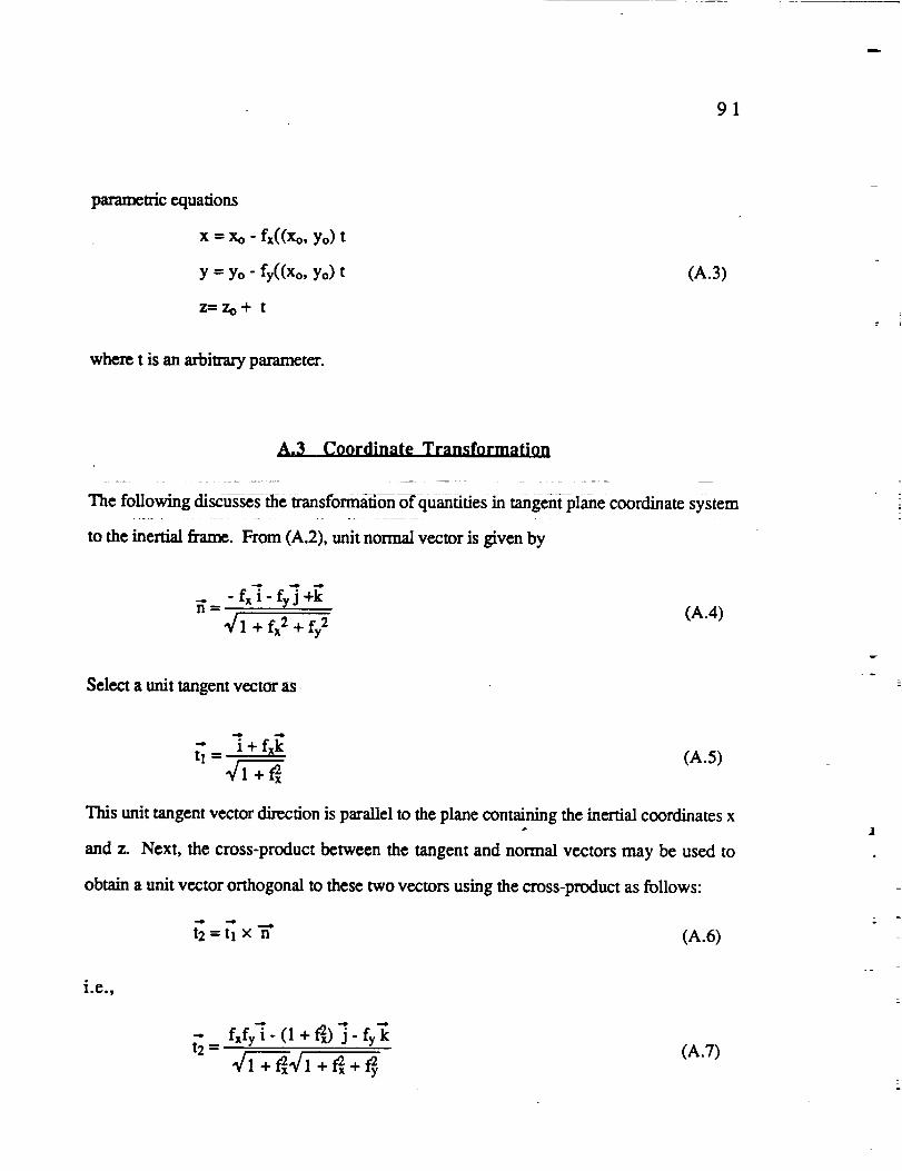
91
parametric equations
x = Xo -fx((Xo,Yo)t
Y = Yo" fy((Xo,Yo)t
Z=Zo+ t
where t is an arbitrary parameter.
(A.3)
A.3 Coordinate Transformation
The following discusses the transformation of quantities in tangent plane coordinate system
to the inertial frame. From (A.2), unit normal vector is given by
_._ -fxi- fyj +k
'_i + fx 2 + fy2
Select a unit tangent vector as
(A.4)
v
(A.5)
This unit tangent vector direction is parallel to the plane containing the inertial coordinates x
and z. Next, the cross-product between the tangent and normal vectors may be used to
obtain a unit vector orthogonal to these two vectors using the cross-product as follows:
.=.o, ,===.O
t2 = tl x n (A.6)
ioe,,
_2- fxfY'_"(I + f2x)_" fY_
1__+ _x41 + _ + _y (A.7)

92
On the tangent plane, the kinematic equations of motion of a particle can be described
as
Xt = V cos X
yt =Vsinx(A.8)
Here, X is the angle made by the velocity vector V with the tangent vector h. Note that the
component of the velocity vector normal to the surface is zero• This is because of the fact
that the vehicle is executing a terrain following flight• The subscript e denotes the local
coordinate system.
The transformation of the velocity vector in the local coordinates system to the inertial
frame may be accomplished using the following:
[:]I ]I 0']x cos (x,,x) cos Lv,,x) cos (z,,x)cos (xt,y) cos (y,,y) cos (zt,y)
cos (x_,h) cos (y,,h) cos (z_,h)(A.9)
The direction cosines can be obtained as
[i].'7" <'_ .'7" _<t 1 , 1> 2, 1> <n, 1>
<t 1, j> <t 2, j> <n, j>
-"
(A.IO)
where <., • > denotes the inner product.
Thus, the kinematic equations of motion over the terrain profile becomes
= Vcos X2
ql +fx
fxfyV sinX
2 +f_I_/_+ fx2_/1 +fx(A.1 I)

93
ql+_ Vsin X
1 + _ +fy2 (A.12)
z - f(x,y) (A. 13)
These equations were used in the trajectory planning schemos discussed in Chapters RI and
IV.
,i

94
APPENDIX B
NUMERICAL CONJUGATE POINT TESTING
FOR FIXED END-POINTS PROBLEMS
B.1 Introduction
The need for conjugate point test in the calculus of variations arise from the
requirement that the second variation evaluated along an optimal path must be greater than
zero for all admissible variations of states and costates. A pointwise test for the sign of
second variation is the well known Legendre-Clebsch necessary condition. For extremals
of f'mite length, however, the task of ensuring that the second variation is positive for all
admissible neighboring paths is more involved [73]. The proposed Jacobi test [97] seeks
the minimum value of the second variation. This problem is called the accessory minimum
problem. The objective here is to find a system of variations which gives the value of zero
to the second variation. If this is possible, it implies that a neighboring path is competitive
and that the extremal furnishes at best an improper minimum of performance index and at
worst merely a stationary value.
Analytical conjugate point test is impossible in all but very simple optimal control
problems. However, a family of numerical methods are available in the literature. This
appendix examines three of these techniques. The first two are very general, while the
third approach is useful in more classical situations such as the optimal trajectory planning

95
problem discussed in Chapter III. All these methods are equivalent, although some are
numerically more efficient than others.
B.2 Second Variation
Consider the general optimal control problem described in Chapter H.
)t = f(x,u,t) ,
Z, =-H x
x(tO = xc
Su -0
H (x,u,X,t) -- L (x,u,t) + _T f (x,u,t)
P (x(tt),t t) -- 0
Q(x(tt.),tf) = g(x(tf),tf) + vTp(x(tf),tf)
(B.1)
(B.2)
(B.3)
(B.4)
(B.5)
(B.6)
(B.7)
S
The augmented performance index is given by:
ja__ Q(x(tf),tf) + {H(x,u,X,t) - xT_} dt
Expanding the augmented performance index 03.8) to second order [12], one has
AJ t = _j a + __ _2j, + higher order terms
(B.8)

96
= Q_x(tf) - _,T(tf)_x(tf) + [(X+Hx) _x+H u _u] dt + xT(t x(tf)
Jto
f' I+21 [_xT _uTI Hxx Hxu _x dt+h.o.t. (B.9)J_ . Hux _ _u
Since the first variation terms vanish along every stationary trajectory, second-variation
becomes
82j a = 8xT(te x(tr)+ [ _ixrHux Huu 5u 03.10)
The differential constraints and boundary conditions in this problem are
= fxSx+ f u,
8x(0) = 0,
8P = [ Px _x]t, = 0
03.11)
03.12)
03.13)
The accessory minimum problem attempts m find the minimum value of the second
variation 03.10) subject to the differential constraints 03.11) and boundary conditions
(B.12), 03.13). The Euler-Lagrange equations for this acc6ssary minimum problem are
given by
5L = - Hr.xSX - fxTsx - Hxu_iu
Hux 8x + fTsx + Huu 8u = 0
_iX(tf) = {gxx + (vrPx)x} 8x [t_
03.14)
03.15)
(B.16)

97
Ifone assumes thatcontrolis nonsingular (i.e.,Huu ;e0), the expression (B.15) may bc
put inthe form
T
8u =-H2_Hu,dSx + fuS_.) (B.17)
In this case, one may substitute for 8u in (B.14) and (B.11) resulting in
I j:EA t,B,t,lE xl8"_L -C(t) -AT(t) 82L (B.I8)
where,
A(t) = fx-fuH_Hux,
B(t) = fuH_u,
C(t) = Hxx- HxuH_I-Iux.
This set of linear differential equations must satisfy the boundary conditions (B. 12),
(B.13), and (B.16).
B.3 The Rieeati Eouation Method
Since the accessary minimum problem (B.18) is linear and the differential equations
and the terminal boundary conditions are homogeneous, both _ix(t) and 8_.(t) are
proportional to 8x(to), or proportional to _iX(tf). Using the backward sweep [41], where in
one assumes a solutionof theform
8_.(t) = S(t) 8x(t), S(tf) = Qxx (8.19)

98
a matrix Riccati equation can be obtained as follows [71]:
_; = - SA -ATS + SBS - C, S(tr)=Qxx (B .20)
Existence of a bounded symmetric-matrix S to the matrix Riccati equation (B.20)
determines the existence of a conjugate point. In other words, if S becomes infinite at any
point t along a test extremal, then the second variation is zero in the interval [to, t]. In such
a case, a neighboring extremal may furnish a lower value of the performance index.
B.4 The Kel!v-Moyer Melhod
Regarding the linearized Euler equations (B. 18) as a mapping between the variations
of unspecified initial costates, 8_.i(0) (i = 1, 2, 3,---, n), and the variations of states, 8xi(t)
(i = 1, 2, 3,.--, n), the following can be written
_X2(t)
_ 8xJt) 8Ln(O)
(B.21)
where _.io m _.i(0), i = 1, 2,..., n.

99
Setting
M(t) =
- ¢3xl o_xl _xl
8Xl0 8X2o 8X.o
_x. O_Xn _xn
m
(B.22)
Kelly [73], Cicala [75], and Moyer [98] showed that the rank of the matrix M(t)
provides the criterion for the existence of a C0njugate point. If the rank of the matrix M(t)
drops at any point along the extremal, it indicates the existence of a conjugate point. In
other words, neighboring extremals starting at to in n-dimensional state space must collapse
into a smaller dimension at a conjugate point
B.S The l_liss Methgd
In Reference 70, a numerical method for conjugate point testing was suggested. For a
two dimensional system, if four fundamental solutions (xi, yi) (i = 1,2,3,4) to the linearized
Euler-Lagrange equations can be obtained, then the determinant of the matrix
d(t) =
Xl x2 x3 x4
Yl Y2 Y3 Y4 (B.23)
£
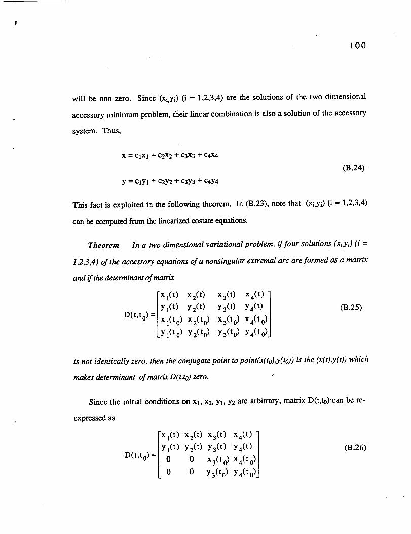
I00
will be non-zero. Since (xi,yi) (i = 1,2,3,4) are the solutions of the two dimensional
accessory minimum problem, their linear combination is also a solution of the accessory
system. Thus,
X --- ClX1 + C2X2 + C3X3 + C4X4
y = clyl + c2Y2 + c3Y3 + c4y4
(B.24)
This fact is exploited in the following theorem. In (B.23), note that (xi.Yi) (i = 1,2,3,4)
can be computed from the linearized costate equations.
Theorem In a two dimensional variational problem, if four solutions (xiYi) (i =
12,3,4) of the accessory equations of a nonsingular extremal arc are formed as a matrix
and if the determinant of matrix
! l(t) X2(t)
1(t) Y2(t)D(t,to) =
1(to) x2(t o)
1(to) Y2(to )
x3(t) x4(t) ]
y3(t) y4(t)./
x3(t 0) x4(to) /
y3(to ) y4(t o)J
(B.25)
is not identically zero, then the conjugate point topoint(x(to),y(to)) is the (x(t),y(t)) which
makes determinant of matrix D(t, to) zero.
Since the initial conditions on xl, x2, Yl, Y2 are arbitrary, matrix D(t,to)'can be re-
expressed as
Ix l(t)
D(t,t 0) = lYl (t) X2(t) X3(t) x4(t)) ]
Y2(t) Y3(t) Y4 (t
0 x3(t 0) X4(t 0)
0 y 3(t0) Y4(t 0)
(B.26)
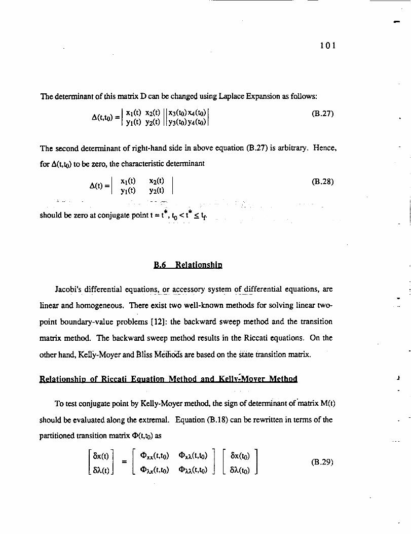
101
The determinant of this matrix D can be changed using Laplace Expansion as follows:
A(t,to)=l Xl(t) x2(t) x3(to)x4(to) 03.27)I yl(t) y2(t) y3(to)y4(to)
The second determinant of right-hand side in above equation (B.27) is arbitrary. Hence,
for A(t, t0) to be zero, the characteristic determinant
i Xl(t) Xz(t)A(t) = ] yl(t) yz(t)
should be zero at conjugate point t = t*, to < t* __<tf.
(B.28)
1
B.6 Relationshio
Jacobi's differential equation_s,or accessory system of differential equations, are
linear and homogeneous. There exist two well-known methods for solving linear two-
point boundary-value problems [12]: the backward sweep method and the transition
matrix method. The backward sweep method results in the Riccati equations. On the
other hand, Kelly-Moyer and Bliss Methods are based on the state transition matrix.
Relationshio of Rie¢ilfi .Eeuation Method and Kellv-'Mover Method
w
J
To test conjugate point by Kelly-Moyer method, the sign of determinant of'matrix M(t)
should be evaluated along the extremal. Equation lB.18) can be rewritten in terms of the
partitioned transition matrix @(t, to) as
@xx(t,t0) @xx(t,t0) ] [ _x(to) ]• xa(t,to) Oxx(t, to) cSX(to)
(B.29)

102
Using the expression (B.21), one can find out that
M(t) = OxX (t,to) (B.30)
From the forward sweep equation, one has [12]
8X,Cto) = S(to) 8X(to) (B.31)
From this,
M-l(t) = S(t,t0) (B.32)
Relationshi_n of Kel!v-Moyer Method and Bliss Method
The following corollary given by Bliss illustrates the relationship between the Kelly-
Moyer method and Bliss method.
Corollary In a two dimensional variational problem, if the accessory equations of
a nonsingular extremal arc are a trajectory of a four-parameter family
x(t,a,b,c,d), y(t,a,b,c,d) (B.33)
then the conjugate point to a point to is determined by the zeros t of the determinant of
matrix
D(t,to) =
x.(t) Xb(t) Xc(t) Xd(t)
y_(t) yb(t) y_(t) yd(t) JXa(lO) Xb(_) Xc(tO) Xd(tO)
ya(tO) yb(t0) yc(t0) yd(tO)
(B.34)
provided that the determinant of matrix D is not identically zero along trajectory.

103
B.7 Numerical Effort
All matrices mentioned in the foregoing axe n by n. Thus, there is no difference in the
size of matrix. To find the existence of conjugate point, however, the first method based on
backward sweep checks the boundedness of a matrix, but the methods based on the
transition matrix, Kelly-Moyer method and Bliss method, check the sign of determinant of
the matrix. The latter approach is numerically better conditioned.
The matrix Riccati method requires the integration of n x n equations and thus
demands a formidable amount of calculations. Primary difficulty here is the requirement
for various partial derivatives. In the present case, this would mean the computation of
higher order terrain gradients.
The numerical evaluati0n 0fthe elements of Keiiy:Moyer method evidently requires
computer codes considerably more complex than those required for the calculation of Euler
solutions. As an alternative to partial derivatives, Menon [99] used a scheme in which the
partial derivatives with respect to the _.io are calculated approximately in terms of difference
quotients. Thus, small increments in the Xio are employed in the evaluation of neighboring
solutions of the extremal.
The numerical Bliss method is similar to the Kelly-Moyer method. Instead of partial
derivatives, fundamental solutions are obtained numerically. As an alternative to
fundamental solutions, in the present work a computer code was assembled based on the
finite differences. This code generates three trajectories corresponding to each heading
angle, the first being the nominal and next two, the neighboring trajectories obtained by
perturbing the initial value of the heading angle by a small amount in the positive and
negative sense. This is equivalent to perturbing the initial values of costates while
wz

104
enforcing the constant of motion. The required fundamental solutions are then computed
using a finite difference scheme.
The main difficulty encountered in both finite difference quotients computations [99]
and finite difference method is the errors arising from higher order effects. These errors
can be controlled to a certain extent by verifying the linearity of the x(t) and Y(0 differences
versus the magnitude of the corresponding increment in the initial heading angle. This
check can be incorporated in the computer program.
If the final end-point is not f'med, the matrix Riccati method requires additional matrix
calculation, see Reference 12 for further details.

w
i

105
APPENDIX C
SEPARABILITY OF THE HAMILTONIAN AND ITS
CONSEQUENCE ON DIFFERENTIAL GAME SOLUTIONS
C.1 Introduction
While discussing the trajectory planning schemes in Chapter W, it was pointed out that
in order to ensure that the outcome of the game is not influenced by the order of action, the
value of the game should exist. The value exists only when the final performance index
has a saddle point. The conditions for the existence of the saddle point are the separability
of the variational Hamiltonian and continuous mapping. In the following, each of these
issues will be elaborated.
C.2 Separability of The Hamiltorlian
p.
Consider a system of differential equations written in vector form
= f (x,d_,W,t), x(t0)=x 0
where, x(t) : = state vector of dimension n, x e X
_(t) : = control of Player 1 of dimension e, _ a
V(t) : = control of Player 2 of dimension m, V _ _F
with terminal constraints:
(C.1)

106
P (x(tf),tf) = 0, tf is free (C.2)
andtheperformanceindexbeingdef'medas
J[x,O,V,t] = g(x(tf),tf ) + L(x,_,V,t) dt (C.3)
The variational Hamiltonian for this problem is given by
H = L + _,T f + l.tiT P + I_2T g (C.4)
If the right-hand side of syStem dynamics (C.1) and the _te6al part of payoff (C.3) are in
the form .......................................... _....
f (x'¢'V't) = fl (x,¢,t) _- f2 (x,v,t) (C.5)
L (x,,,V,t) = L 1 (x,O,t) + L 2 (x,v,t) (C.6)v
then the Hamiltonian is separable in the space of controls _ and O as follows:
H = H I + I-I2 + _tzT P + Ix2T g
H I = L I (x,¢,t) + _T fl (x,¢,t)
H2 = L2 (x,V,t) + _T f2 (x'V,t)
(C.7)
(C.8)
(C.9)
In this case, Friedman [39] showed that there exists a saddle point for the Hamiltonian.
The order of action is immaterial in this case, i.e.,
O Omax min H(x,¢,W,X,t) = rain max H(x,¢,¥,X,t)= H(x,¢ ,V ,X,t)
¥ ¢ ¢ ¥
(C.I0)

107
Equation (C.10) is known as the Isaacs condition in differential game [39]. This condition
is also known as the saddle point condition.
C.3 Sufficient Condition for a Game to have Value
As discussed in the previous section, the Isaacs condition guarantees the existence of
the pointwise saddle point. If the final performance index in the game has a saddle point,
then one is guaranteed that the order of action is immaterial. This section treats how the
pointwise saddle point can be transformed to the global saddle point. The chief
requirement here is that the game must have a value.
Friedman [39] [100] proved that a sufficient condition for the game to have a value is
the Isaacs condition and the following requirements,:
(i) f(x,_,_,t) is continuous and satisfies the Lipschitz condition,
(ii) g(x(tr), tf) and L(x,¢,_g,t) are continuous.
Here, condition (i) is required so that the trajectory generated by integrating equations of
motion (C. 1) is unique and continuous, while condition (ii) is required to ensure that the
performance index is continuous. Under these conditions, if the variational Hamiltonian is
separable, the performance index will be a unique quantity regardless of the player's order
of action.
To show the existence of the value, Friedman [39] and Fleming [101] considered an
approximating upper and lower game for every partition of the time interval [to, tf] into K
equal sub-intervals. Using the requirement (i), the trajectory evolves according to

108
f(x,_jJgj,x)dx(C.11)
Two possibilities are next considered. The first one in which the minimizing player
plays first. In the second case, the maximizing player plays first. The performance index
ineachcaseis
+
V K --inf sup.-- inf sup J[x,_j,_l/j,t ] j=0,1,2,...,K-1_0 00 O,t-t Vz-!
VK- =sup inf • .-sup inf J[x,0j, Wlt] j=0,1,2,.--,K-1#0 "ll/O 'tj/r _I 1_ r--I
(C.12)
(C.13)
With the increment of K,
4- +
lim VK--V , lira V i V-K--_ K---_
It can be shown [39] that in the general case,
(C.14)
V + >V" (C.15)
Note that the above expression will be an equality if the Isaac's condition is satisfied. In
such a case,
O Omax rain J[x,_,lg,t] - rain max J[xAb,lg,t ] = J[x,_) ,_ ,t] (C.16)
v # ¢ v

109
APPENDIX D
CONVEXITY CONDITION FOR GLOBAL MINIMUM
Convex functionals play a special role in optimal control theory because most of the
theory of local extrema for general nonlinear functionals can be strengthened to become
global theory when applied to convex functionals [69].
By def'mition in Reference 35, a real-valued functional J: Y ---> 9_ is convex if
J[ot Yl + (1 - tz) Y2] < a J[yl] + (1 - ¢z) J[y2], V yl,y2 _ Y, 0 < a < 1 (D.1)
The following theorem [35] asserts the global nature of results for minimization problems
with convex functionals such as those defined in (D. 1).
Theorem If J(Yo) is a weak local minimum of J(y) on Y and J is convex at Yo relative
to Y, then J(Yo) is a global minimum.
A sufficient condition for convexity of functionals is that the integrand be convex for
the integral interval. Thus the test of convexity for a functional can be reduced to a test of
the convexity of the integrand. Typical integrands that are convex appear in Linear
Quadratic Regulator theory and in the accessory minimum problem related to the Jacobi
condition in nonsingular cases.

w.
z _

110
BIBLIOGRAPHY
[11
[2]
[3]
[4]
[5]
[6]
[7]
Sheridan, P. F., and Wiesner, W., "Aerodynamics of Helicopter Flight Near
the Ground," The 33rd Annual National Forum of the American Helicopter
Society, Washington, D.C., May, 1977, Preprint No. 77.33-04.
Dooley, L. W., "Handling Qualities Considerations for NOE Flight," Journal
of the American Helicopter Society, Vol. 22, No. 4, October, 1977, pp. 20-27.
Landis, K. H., and Aiken, E. W., "Simulator Investigation of Side-Stick
Controller/Stability and Control Augmentation Systems for Night Nap-of-Earth
Flight," Journal of the American Helicopter Society, Vol. 29, No. 1, January,
1984, pp. 56-65.
Sridhar, B., and Phatak, A. V., "Simulation and Analysis of Image-Based
Navigation System for Rotorcraft Low-Altitude Flight," The AHS National
Specialists '_Meeting Automation Applications of Rotorcraft, Atlanta, GA, April
4-6, 1988.
Cheng, V. H. L., and Sridhar, B., "Considerations for Automated Nap-ofothe-
Earth Rotorcraft Flight," proceedings of American Control Conference. Vol. 2,
Atlanta, GA, June 15-17, 1988, pp. 967-976.
Cheng, V. H. L., "Obstacle-Avoidance Automatic Guidance," Proceedings of
AIAA Guidance. Navigation and Control Conference. Minneapolis,' Minnesota,
August 15-17, 1988.
Denton, R. V., Jones, J. E., and Froberg, P. L., "A New Technique for
Terrain Following/Terrain Avoidance Guidance Command Generation,"
AGARD-CP-387, 1985.
111
[S] Doff, D. W., "Rotary Wing Aircraft Terrain-Following/Terrain-Avoidance
System Development," Proceedings of AIAA Guidance. Navigation and
Control Conference. Williamsburg, VA, August 18-20, 1986, Paper No. 86-
2147.
[9] Hoffman, J. D., "Terrain Following/Terrain Avoidance/Threat Avoidance for
Helicopter Applications," American Helicopter Society Mideast Region
Procee&'ng National Specialists' Meeting, CherryI-Ifll, New Jersey, October 13-
15, 1987.
[10] Gilmore, J. F., and Semeco, A. C., "Knowledge-Based Approach Toward
Developing an Autonomous Helicopter System," Optical Engineering, Vol. 25,
March, 1986, pp. 415-427.
[11] Olinger, M. D., and Bird, M. W., "Tactical Flight Management: Threat
Penetration Algorithm Design," Proceedings of IEEE 1984 National Aerospace
Electronics Conference, Dayton, OH, May 21-25, 1984, pp. 510-515.
[12] Bryson, A. E., and Ho, Y. C., Applied Optimal ContrQ1. Hemisphere, New
York, 1975.
[13] Menon, P. K. A., Kim, E., and Cheng, V. H. L., "Helicopter Trajectory
..... P!anningUs_g_timal Control Theory,'_oeeedings of the 1988American
- Controi Conference_ V0[ 2, Atlanta,GA,_June i5:i7, i988, ppl 1440-1447.
[14] Zermelo, E., "Uber das Navigationsproblem bei ruhender oder ver_derlicher
Windverteilung," Zeitschrift f'tir angewandte Mathematik und Mechanik, Bd.
11, 1931.
[15] Menon, P. K. A., Kim, E., and Cheng, V. H. L., "Optimal Terrain Masking
Trajectories for Helicopters," AIAA Guidance, Navigation and Control
Conference, Minneapolis, MN, August 15-17,1988.
[16] Nayfeh, A. H., Introduction to Perturbation Techniques, John Wiley & Sons,
Inc., New York, 1981.

112
[17]
[18]
[19]
[20]
[21]
[22]
[23]
[24]
[25]
[26]
Isaacs, R., Differential Games, John Wiley & Sons, New York, 1965.
Menon, P. K. A., "Short-Range Nonlinear Feedback Strategies for Aircraft
Pursuit-Evasion," Journal of Guidance, Control, and Dynamics, Vol. 12, No.
I, Jan-Feb, 1989, pp. 27-32.
Heiges, M. W., "A Helicopter Flight Path Controller Design via a Nonlinear
Transformation Technique," Ph.D. Dissertation, Georgia Institute of
Technology, Atlanta, GA, March, 1989.
Lewis, M. S., Mansur, M. H., and Chen, R. T. N., "A Piloted Simulation of
Helicopter Air Combat to Investigate Effects of Variations in Selected
Performance and Control Response Characteristics," NASA TM 89438,
August, 1987.
Lewis, M. S., and Aiken, E. W., "Piloted Simulator of One-on-One Helicopter
Air Combat at NOE Flight Levels," NASA TM 86686, April, 1985.
Pugh, G. E., and Krupp, J. C., "A Value-Driven Control System for the
Coordination of Autonomous Cooperating Underwater Vehicles," Unmanned
system, V01. 6, No. 2, 1988, pp. 24-35.
Crowley, J. L., "Navigation for an Intelligent Mobile Robot," IEEE Journal of
Robotics and Automation, Vol. RA-1, No. 1, March, 1985, pp. 31-41.
Reed, C. G., and Hogan, J. J., "Range Correlation Guidance for Cruise
Missiles," Proceedings of IEEE 1978 National Aerospace Electronics
_, Dayton, OH, May 16-I8, 1978, pp. 1255-1262.
Kupferer, R. A., and Halski, D. J., "Tactical Flight Management-Survival
Penetration," Proceedings of rEEE 1984 National Aerospace Electronics
Dayton, OH, May 21-25, !984, pp. 503-509.
Fleury, P. A., "Covert Penetration Systems-Future Strategic Aircraft Missions
Will Require a New Sensor System Approach," Proceedings of IEEE 1986
I
113
[27]
National Aerospace Electronics Conference. Dayton, OH, May 19-23, 1986,
pp. 220-226.
Bellman, R., Dynamic Pro_ammin_. Princeton University Press, Princeton,
N. J., 1957.
[28] Winston, P. H., Artificial Intelligence, Addison-Wesley Pub., Reading, MA,
1984.
[29]
[30]
[31]
[32]
[33]
Denton, R. V., and Marsh, J. V., "Applications of Autopath Technology to
Terrain/Obstacle Avoidance," Proceedings of IEEE 1982 National Aerospace
Electronics Conference. Dayton, OH, May 18-20, 1982, pp. 1373-1377.
Chart, Y. K., and Foddy, M., "Real Time Optimal Flight Flight Path
Generation by Storage of Massive Data Bases," Proceedings of IEEE 1985
National Aerospace Electronics Conference, Dayton, OH, May 20-24, 1985,
pp. 516-521.
Austin, F., et al., "Automated Maneuvering Decisions for Air-to-Air Combat,"
Proceedings of 1987 AIAA Guidance. Navigation. and Control Conference.
Monterey, CA, Paper Preprint 87-2393.
Von Neumann, J., and Morgenstern, O., Theory of Games and Economic
Princeton University Press, Princeton, 1944.
Pontryagin, L. S., Boltyanskii, V. G., Gamkrelidze, R. V., and Mishchenko,
E. F., The Mathematical Theory of Optimal Process, The Macmillan Company,
New York, 1964.
[34] Pierre, D. A., Optimization Theory with Applications, Dover Publications,
N.Y., 1986. _ )_ ..........
[35] Ewing. G. M,, Calculus ofVafiati0n with Applications. Dover Publication.
New York, 1969:
[36] ....H--o,Y. C., "Review-0f Differential Games, by R. Isaacs," IEEE Trans. on
Automatic Control, Vol. AC-10, No. 4, October, 1965, pp. 501-503.

[,
114
[37]
[38]
[39]
[401
[41]
[42]
[43]
[44]
[45]
[46]
[47]
Berkovitz, L. D., and Fleming, W. H., "On Differential Games With Integral
Payoff," Annals of Math. Study, No.39, Princeton University Press,
Princeton, 1957, pp. 413-435.
Berkovitz, L. D., "A variational Approach to Differential Games," Annals of
Math. Study, No. 52, Princeton University Press, Princeton, 1964, pp. 127-
173.
Friedman, A., Differential Games, Wiley-Interscience, New York, 1971.
Start, A. W., and Ho, Y. C., "Nonzero-Sum Differential Games," Journal of
Optimization and Applications, Vol. 3, No. 3, 1969, pp. 184-206.
Simaan, M., and Cruz, J. B., "On the Stackelberg Strategy in Nonlinear-Sum
Games," Journal of Optimization and Applications, Vol. 11, No. 5, 1973, pp.
533-555.
Berkovitz, L. D., Optimal Control Theory, (Applied Mathematical Sciences,
Vol. 12), Springer-Verlag, New York, 1974.
Ho, Y. C., Bryson, A. E., and Baron, S., "Differential Games and Optimal
Pursuit-Evasion Strategies," IEEE Trans. on Automatic Control, Vol. AC-10,
No. 4, October, 1965, pp. 385-389.
Basar, T., and Olsder, G. J., Dynamic Noncooperative Game Theory,
Academic Press, New York, 1982.
Kailath, T., _, Prentice-Hall Inc., New Jersey, 1980.
Wonham, W. M., Linear Multivarable Control: A Geometric Approach, 2nd
Ed., Springer-Verlag, New York, 1979.
Krener, A. J., "On the Equivalence of Control Systems and the Linearization of
Nonlinear Systems," SlAM Journal of Control, Vol. 11, No. 4, November,
1973, pp. 670-676.
115
[48]
[49]
[50]
[51]
[52]
[53]
[54]
[55]
[56]
[57]
Brockett, R. W., "Feedback Invariants for Nonlinear Systems," Proceedings of
IFAC Worm Congress, Helsinki, Finland, 1978, pp. 1115-1120.
Ball, W. W. R., A Short Account of the History_ of Mathematics, Dover
Publications, New York, 1960.
Meyer, G., "The Design of Exact Nonlinear Model Followers," Joint Automatic
Control Conference, FA-3A, 1981.
Sussmann, H. J., "Lie Brackets, Real Analyticity and Geometric Control,"
Differential Geometric Control Theory, Proceedings of the Conference hem at
MiJiig-ah Technologicat unlversity, June 28 - July 2, 1982, pp. 1-116.
Hunt, L. R., Su, R., and Meyer, G., "Global Transformations of Nonlinear
Systems," IEEE Transactions on Automatic Control, Vol. AC-28, No. 1,
January, 1983, pp. 24-30.
Hunt, L. R., and Su, R., "Control of Nonlinear Time-Varying systems,"
Proceedings of IEEE Conference on Decision and Control. San Diego, CA,
1981, pp. 558-563.
Su, R., "On the Linear Equivalents of Nonlinear Systems," Systems and
Control Letters, Vol. 2, No. 1, July, 1982, pp. 48-52.
Meyer, G., and Cicolani, L., "Application of Nonlinear System Inverses to
Automatic Flight Control Design-System Concepts and Flight Evaluations,"
AGARDograph 251 on Theory and Applications of Optimal Control in
Aerospace Systems, 1980.
Meyer, G., Hunt, R. L., and Su, R., "Design of Helicopter Autopilot by
Means of Linearizing Transformations," Proceedings of Guidance and Control
Panel 35th Symposium, AGARD-CP -321, 1983, pp. 4.1-4.11.
Meyer, G., Su, R., Hunt, R. L., "Application of Nonlinear Automatic Flight
Control," Automatica, Vol. 20, No. 1, 1984, pp. 101-107.
116
[58]
[59]
[60]
[61]
[62]
[63]
[64]
[65]
[66]
[67]
[68]
Menon, P. K. A., Badgett, M. E., Walker, R. A., and Duke, E. L., "Nonlinear
Flight Trajectory Controller for Aircraft," Journal of Guidance, Control, and
Dynamics, Vol. 10, No. 1, Jan-Feb 1987, pp. 67-82.
Heiges, M. W., Menon, P. K. A., and Schrage, D. P., "Synthesis of a
Helicopter Full Authority Controller," proceedings of the AIAA Guidance.
Navigation and Control Conference, Boston, MA, August 14 - 16, 1989, Part
1, pp. 207-213.
Lee, E. B., and Markus, L., Foundations of Optimal Control Theory. Wiley,
New York, 1967.
Bogen, R., et al., MACSYMA Reference Manual, Version 10, The Mathlab
Group Laboratory for Computer Science, M.I.T., Cambridge, MA, 1983.
Conte, S. D., and de Door, C., Elementary_ Numerical Analysis, McGraw Hill,
N.Y., 1980.
U.S. Geological Survey, San Andreas. California: N3800-W12030/15, AMS
1860II-Series V795, Denver, CO, 1962.
Rogers, D. F., and Adams, J. A., Mathematical Elements for Computer
Graphics, McGraw Hill, N.Y., 1976.
Kelley, H. J., "Reduced Order Modelling in Aircraft Mission Analysis", AIAA
J., Vol. 9, 1972, pp. 349-350.
Kelley, H. J., "Aircraft Maneuver Optimization by Reduced Order
Approximation," Control and Dynamics, Vol. 10, edited by C.J. Leondes,
Academic Press, N. Y., 1973, pp. 131-178.
Calise, A. J., and Moerder, D. D., "Singular Perturbation Techniques for Real
Time Aircraft Trajectory Optimization and Control," NASA'CR-3597, 1982.
Gelfand, I. M., and Fomin, S. V., Calculus of Variations with Application,
Prentice-Hall, N. J., 1963.
117
[69] Luenberger, D. G., Optimization bv Vector Space Methods, John Wiley &
Sons, Inc., New York, 1968.
[70]
[71]
Bliss, G. A., Lectures on the Calculus of Variations. Univ. of Chicago, 1946.
Breakwell, J. V., and Ho, Y. C., "On the Conjugate Point Condition for the
Control Problem," International Journal Engineering, Vol. 2, 1965, pp. 565-
579.
[72] BreakweU, J. V., Speyer, J. L., and Bryson, A. E., "Optimization and Control
of Nonlinear Systems Using the Second Variations," Journal of SIAM Control
Series A, Vol. 1, No. 2, 1963, pp. 193-223.
[73] Kelley, H. J., and Moyer, H. G., "Computational Jacobi Test Procedure,"
JUREMA Workshop, Dubrovnik, Yugoslvia, June 29-30, 1984.
[74] Hildebrand, F. B., Advanced Calculus for Applications, Prentice-Hall, Inc.,
New Jersey, 1976.
[75] Cicala, P., An Engineerin_ Atmroach to the Calculus of Variations. Libreria
_trice Univ., Torino, Italy, 1956.
[76] Bolza, O., Lectures on the Calculus of Varialions, Dover Publications, N.Y.,
1961.
v
[77]
[78]
[79]
Ciletti, M. D., and Starr, A. W., "Differential Games: A Critical View,"
Differential Games: Theory_ and Applications. 1_70 Joint Automatic Control
Conference, Atlanta, GA, June 26, 1970, pp. 1-17.
Lappos, N. D., "The LHX-Evolved for Total Combat Fitness," VERTIFLITE,
Vol. 35, No. 5, July/August, 1989, pp. 16-17.
Breakwell, J. V., and Merz, A. W., "Toward a Complete Solution of the
Homicidal Chauffeur Game,"Pr0ceedines o_isi international Conference on
the Theory. and Application of Differential Games, Amherst, Mass., 1969, pp.
III-1 - 111-5.
118
[80]
[81]
[82]
[83]
[84]
[85]
[86]
[87]
[88]
[89]
Merz, A. W., "The Homicidal Chauffeur," A/AA Journal, Vol. 12, No. 3,
March, 1974, pp. 259-260.
Merz, A. W., "To Pursue or to Evade-That is the Question," Journal of
Guidance, Control, and Dynamics, Vol. 8, No. 2, 1985, pp. 161-165.
Flight Systems, Inc., "Helicopter Effectiveness in Air-to-Air Combat," U.S.
Army Aviation Research and Development Command, Contract No. NAS2-
10239, 1979.
Buresh, J., Parlier, C., and Wilson, W., "Air-to-Air Combat Development of
the AH-64A Apache," Proceedings of AIAA 4th Flight Test Conference, San
Diego, CA, May 18-20, 1988, pp. 268-277.
Rajan, N., Prasad, U. R., and Rao, N. J., "Pursuit-Evasion of Two Aircraft in
a Horizontal Plane," Journal of Guidance and Control, No.3, May-June, 1980,
pp. 261-267.
Leondes, C. T., ed., Control and Dynamic Systems: Advances in Theory and
Applications, Vol. 17, 1981.
Prasad, U. R., Rajah, N., and Rao, N. J., "Planar Pursuit-Evasion with
Variable Speeds, Part 1, Extremal Trajectory Maps," J. Optimization Theory
and Applications, Vol. 33, No. 3, March, 1981, pp.401-418.
Rajan, N., and Ardema, M. D., "Barriers and Dispersal Surfaces in Minimum-
Time Interception," J. Optimization Theory and Applications, Vol. 42, No. 2,
February, 1984. pp. 201-228.
J_irmark, B. S. A., "Convergence Control in Differential Dynamic
Programming Applied to Air-to-Air Combat" A/AA Journal, Vol. 14, No. 1,
January, 1976, pp. 118-121.
Roberts, D. A., and Montgomery, R. C., "Development and Application of a
Gradient Method for Solving Differential Games," NASA-TN-D-6502,
November, 1971.

119
[90]
[91]
[92]
[93]
[94]
[95]
[96]
[97]
[98]
Shinar, J., "Validation of Zero-Order Feedback Strategies for Medium-Range
Air-to-Air Interception in a Horizontal Plane," NASA TM-84237, April, 1982.
Riggs, T. L., "Linear Optimal Guidance for Short Range Air-to-Air Missiles,"
Proceedings of IEEE 1979 National Aerospace Electronics Conference, Dayton,
OH, May 23-27, 1979, pp. 757'764.
Lee, G. K. F., "Estimation of the Time-to-Go Parameter for Air-to-Air
Missiles," Journal of Guidance, Control, and Dynamics, Vol. 8, No. 2, 1985,
pp 262-266
Menon, P. K. A., Calise, A. J., and Leung, S. K. M., "Guidance Law for
Spacecraft Pursuit-Evasion and Rendezvous," A/AA Guidance, Navigation and
Control Conference, Minneapolis, MN, August 15-17, 1988.
Talbot, P., Tingling, B., Decker, W., and Chen, R., "A Mathematical Model of
a Single Main Rotor Helicopter for Piloted Simulation," NASA TM 84281,
September, 1982.
Kant, K., and Zucker, S., "Planning Collision-Free Trajectories in Time-
Varying Environments: A Two-Level Hierarchy," Proceedings of IEEE
Conference on Robotics and Automation, Vol. 3, Philadelphia, Pennsylvania,
April 24-29, 1988, pp. 1644-1649.
Khatib, O., "Real-Time Obstacle Avoidance for Manipulators and Mobile
Robots," The International Journal of Robotics Research, Vol. 5, No. 1, 1986,
pp. 90-98.
Fox, C., An Introduction to the Calculus of Variations, Dover Publications,
New York, 1987.
Moyer, H. G., "Optimal Control Problems That Test for Envelope Contacts,"
Journal of Optimization Theory and Applications, Vol. 6, No. 4, 1970, pp.
287-299.
120
[99] Menon, P. K. A., "Optimal Symmetric Flight with an Intermediate Vehicle
Model," Ph. D. Thesis, Virginia Polytechnic Institute and State University,
Blacksburg, VA, September, 1983.
[100] Roxin, E. O., "On Differential Games Without Value," Differential Games:
Theory. and Applications. 1970 Joint Automatic Control Conference, Atlanta,
GA, June 26, 1970, pp.95-119.
[101] Elliott, R. J., "Introduction to Differential Games," The Theory_ and Application
of Differential Games, (Grote, J. D., ed.) Proceedings of the NATO Advanced
Study Institute held at University of Warwick, Coventry, England, August 27-
September 6, 1974.


121
o.
• ==
• • • • • • • • = = • • • • • • • • , •
• .____ ...... _ ......
_. _. _. ',_. . _. _. _ _. r-:. _ _ _. ,.n._ r':. _. _ _ _

122
rot,
Table 5.1 Maximum Rate of Climb (ft/scc_ for AH-1S
Speed (ft/sec)
0
16.67
33.33
50
66.67
83.33
100
116.67
133.33
150
166.67
183.33
200
216.67
233.33
250
DensityAltitude
sealevel I000 ft 2000 ft
22.2 21.25 20.22
25.21 24.65 24.02
29.08 28.63 28.13
32.25 31.9 31.52
34.43 34.2 33.92
35.6 35.43 35.25
35.91 35.82 35.7
35.42 35.43 35.37
34.23 34.27 34.28
2.27 32.38 32.47
29.52 29.7 29.87
25.9 26.18 26.43
21.38 21.78 22.12
15.9 16.42 16.67
8.77 8.72 8.58
0 0 0
3000 ft
19.1
23.35
27.58
31.1
33.6
35.02
35.53
35.23
34.25
32.5
29.97
26.62
22.4
16.32
8.37
0
v
r../t-

123
z_
IH \ /-- TANGENT PLANE ROFILE
X
Figure 3.1 The Coordinate System
V

INITIAL GUESS
= ATAN F yf" y(O)X(0) XoL xf- x(O)
INTEGRATE DIFFERENTIAL EQUATIONS
i,_,_FORWARD TILL x(tf) = xf
_ INPI.rI"
x(O) , y(O)
xf, yf
Z rain' Z max
]
124
COMPUTE CROSS-RANGE ERROR
e = y(tf)-yf
Xo=x,,+Axj YES
NO
P
DE_[_----_ Ax BASED ON
METHOD OF BISECTIONS
X max AND X. ,-,1inTO BOUND
SEARCH RAN__._
OFTIMAL
SOLUTION FOUND
T
.I
Figure 3.2 Flow Chart for Generating Euler Solutions

125
Figure3.3SampleTerrainMapof theNassau-Valley,California

I
126
_TrrCU_Et_rr:FEET " f \..--- : _ ,'1",;'I/l,,:,,/,,'13,IDATI._:MEANSEAI._VIEL ,, "_ ; I ,'I _ _, :[ ,"/_"'( [SmEnm,_GTI-I.2o.ooo_ -.. /' I." ",_7-. _I _.', .- -,..
/ \o ', /,."/," ..'7-',._ _ ',,' "-:/
/ ," , "_ i ' P ' # /t _ , _ o_" t,' /I ," i A\ _ I , / / II _ I , I # " f- ..i ,,. ,,/\\ : r,, (jl,.. _', :i,'f/.-'_,
i . i / ) \ _ , _.v I , - I _ ,I' ,,__i ,/./ , .'/ / \ I ' /./ "',_I ,'C._.--L;-'T.-f.
.'-.._---'I _/ \ , , : ,----1-' ', _', ,',_.--_.-:" _ "--"-"- _ _ _ , l I I_ I _ "f.,/_.'/
, /'_ : _ : , # ', t ',\'.._/_i/ \ '1 ,,.._../. :\ ,,._./-'-
; _ i \ e,q3 ,, ,I ", ,--., ,, k,f-_._._......, _ i _,_:,.,--, r_ ,I.. , ," : ,,/.v¢---_..- -..
_.' "--J .----;_-,.U ll_ :'--_'- : /, .: ._,o'_'-..," ,_.."_/Xc_,',A'_/.:./" ": \ /:".i.. _"" :'/_'_I"I.';:-->/..-""-/
/ _ :.i/.//:W'.,_o.....---: ..."k:'/:,'" V,_.°_.,''/-\ _.-;_ ../ ....... "
:-\ '..>7".:: I ..--:,:oe._o.......
....' :2.,---,, Y/ ....
v
Ai
Figure 3.4 Euler Solutions for Minimum Flight Time Criterion (K = 0)
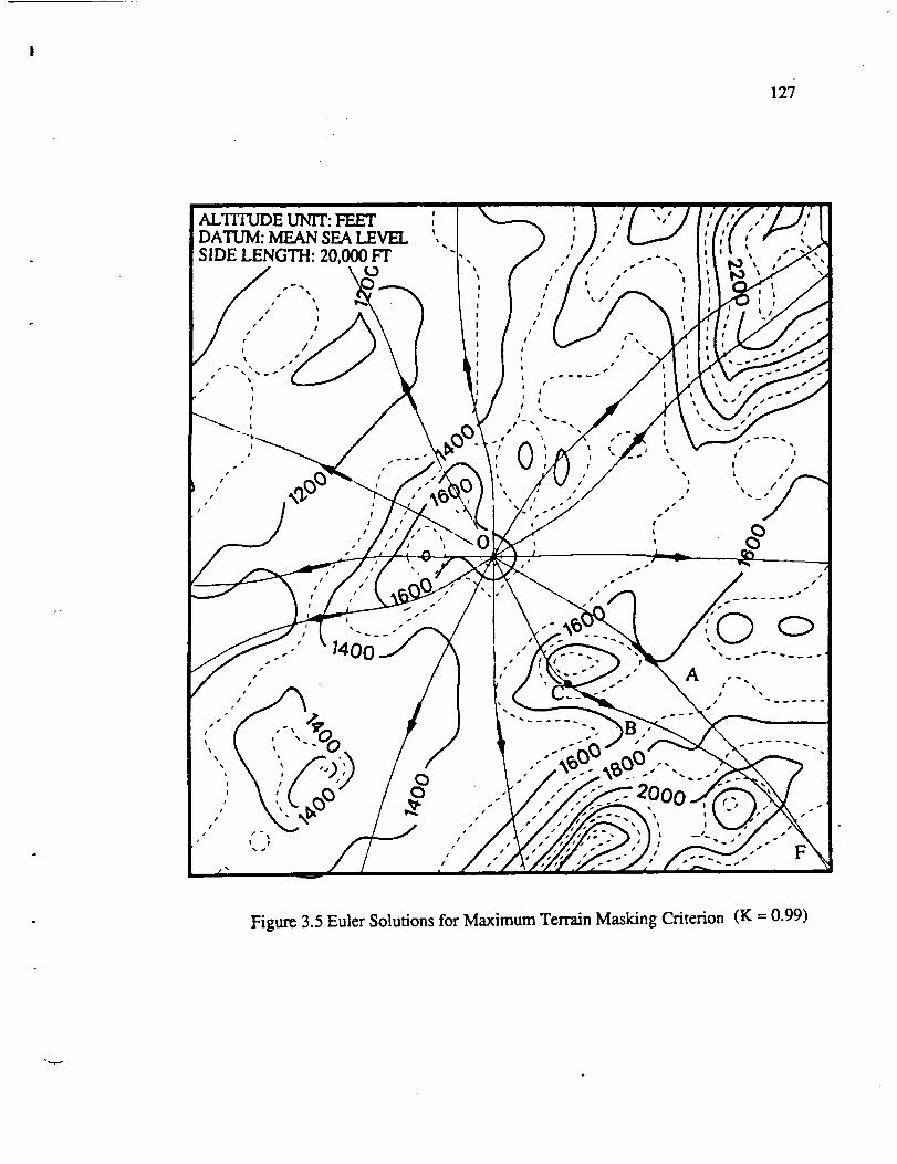
127
AL'ITrUDE UNIT: FEETDATUM: MEAN SEA LEVEL ',SIDE LENGTH: 20,000 FT
I •
E t
J I
I
, ]JI
I %
I
!
f
¢
/
p •
I
I
• % Is !
I •!
I •
! •I
t •
%
%
As I •
F
Figure 3.5 Euler Solutions for Maximum Terrain Masking Criterion (K = 0.99)

128
ALTITUDE UNIT: FEETDATUM: MEAN SEA LEVELSIDE LENGTH: 20,000 l_
jI p_..
.,," ,(,I,00/ ,"-"
I
t
!
t'
v
Figure 3.6 Comparison between Minimum Time Trajectoryand Maximum Terrain Masking Trajectory

129
2m
<
2000
1900
1800
1700
1600
1500
140010000
I lI I
I II
IIIIII
II
II
I
IIII
/
!
11 000 12000 13000 14000 15000 16000
Down-range (feet)
Figure 3.7 Altitude Profiles along Different Criterion TrajectoriesSolid line:maximum terrain masking trajectory
Dotted Line:minimum flight time trajectory

130
0.000
-0.005
-0.010
-0.015
-0.020
-0.025
-0.030
0
=
-20
| rr | I
10 20
I o I , ! , I , I i
10 20 30 40 50 60
w
=
Time (sec)
Figure 3.8 Characteristic Determinant A(t) along the Trajectory A
for Maximum Terrain Masking (K = 0.99)
1
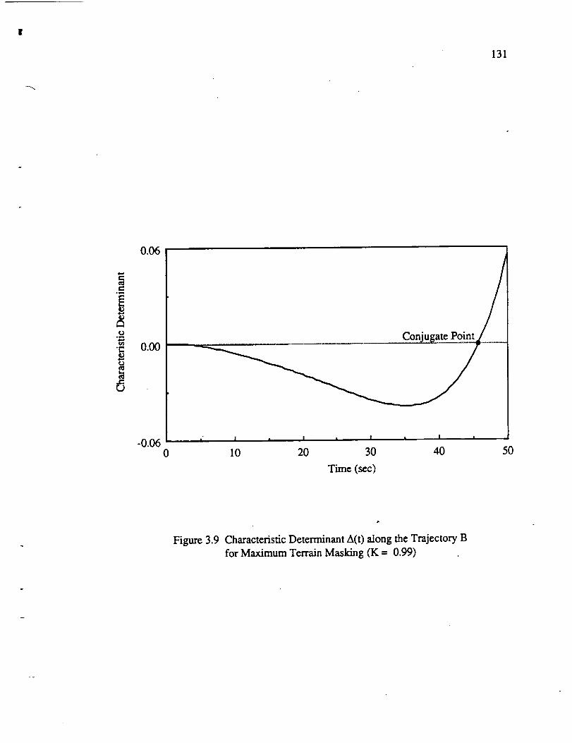
131
0.06
0
•_ 0.00
Conjugate Poi
-0.06 , I , ' , I , ' ,0 10 20 30 40
Time (sec)
50
Figure 3.9 Characteristic Determinant A(t) along the Trajectory B
for Maximum Terrain Masking (K = 0.99)

132
¢19
t-in
r,9e-
300000
200000
100000
Trajectory A
Trajectory B
0 I i ! . L... I . I
tJO00 10000 12000 14000 16000 18000 20000
Down-range (feet)
Figure 3.10 Comparison of Performance Index along Trajectories A and Bfor Maximum Terrain Masking

133
ALTITUDE UNIT: FEET : _ ', _ //' ",;") [ ,"/,'7". //_.J/ iDATUM: MEAN SEA LEVEL '. "_ ] / ' [ _ ['[,'( _" r- '. 1SIDE LENGTH: 20,000 FEET .. I/ , /. _ i, [:[_', ..--.
/ o ", f ,./: .. ,,I,,\_,,,/.-.. _w_ , l , / ', ,._ , /',_0 :',
/ ,. , ,t..vx _ } ,' / -- ,f _ , _,/o, , ..,z 'i I ¢ I [ l
i I I I l t I t .r
/ ', .:/ // ', I ; / "', l,/,\'.---_z.z_.-'D,.'-'.,'---'/ / I , I ', ...... " ;I ,/,kfT3--_2.2_.-:
' f I I 1 I 'i _'" g#
I 1 l l, I x s
. _ ,.,o , , ", ..---,', \M.d,d...... .; / . I'i) ',9 --', r_ , ^ , ,. , ', _, ",
• / __-- _ , I I _ 1% '. "--- , ' ,,'.-- _I ,,"-_./.i"m ,, w , ;) ,, ", t ,,__
, _0 , f."/___ , , V , , ,. / f-_) ; i_ll_jii ) # _ f.( _ ] • l +, t • , l
- _1.' , l ' "_110v ] , , .-" ." "- /" 1 ,,/,"/i. 'L -;- ,' -"
s ,I.i.-" X ' , 0.- ///," ', __'_X , O ,.- ,' ,,o, O, .' ,'/ - .. /,/,,.c/....,,o._ >. .. ,
/ /_'_ ,./.:( ;;<," ....,,,__,_. ...- / ..,-_ '_..!:.,,,@7. - _ ..:_ ! ......."1 O- " ....
#
."".../5 " ! '. (-.._L_.:",A .-' ""......," / _ t "- ...... -.,'%, ,.'---"_-,,,,-,_oo ) .:-_'_>P-../..--,. \ ,,<.,_ _, ...-;,o?__,,_,:>%......;._._"-_,
£ .-.---"-- ........ -/., ./:__o./_-:,}....x v_ . ,.//.._/,;,/_,d.,_-._.,\ ',k._,¢/-/ .."
. ::- _ ..' / /,h;//_-_? :).:..._-.U4.-<., _/ . /, /.-,:w.><.---.i'..,<.._----
Figure 3.11 Two Extremals for Minimum Flight Time Criterion
having a Same Terminal Position

134
0.04
.! 0.00
-0.040
I" • ! • ! • I
10 20 30 40
Time (sec)
50
Figure 3.12 Characteristic Determinant A(t) along the Trajectory A
for Minimum Flight Time (K = 0.0)
3c
ip

135
0.00
i-0.04
-0.08
li
| !
0
I " I I i I I
10 20 30 40
Time (see)
50
Figure 3.13 Characteristic Determinant A(t) along the Trajectory B
for Minimum Flight Time (K = "0.0)

1
136
FEETDATUM: MEAN SEA LEVEL
SIDE LENGTH: 20,000 FT
s
2000
/!
I
/
C>
Figure 3.14 Euler Solutions for Optimal Route Planning No.2
(or = 10"'5, _ --0.001)
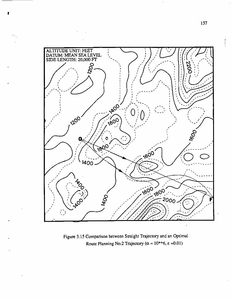
137
fALTITUDE UNIT: FEETDATUM: MEAN SEA LEVEL '
%
SIDE LENGTH: 20,000 FT "-.O
,. ,_o° /
#
t
Figure 3.15 Comparison between Straight Trajectory and an Optimal
Route Planning No.2 Trajectory (or = 10"'6, E =0.01)

138
I
m
<
2400
22OO
2OOO
1800
1600
1400
1200bOO0
Optimal Trajectory
Straight Trajectory
10000 15000 20000
Down-range (feet)
v
Figure 3.16 Altitude Profiles along Straight Trajectory and Optimal Trajectory

139
ALTITUDEUN1T:FEET ' I \_..--- '. _ :[ "';'/] "I,,7","/J,"[
DAtUM:MEaNSEALEVEL', ? 3 : ) ," _ d:'J'(: _"i tSIDE LENGTH: 20,000FT "-.. ' / / /.. -__ 1,1 I ,, .-.:..
/ \o , f..I," .-"1-', , ,o,, ,.!.-. \0..-._ , ," I '. ,'d ', ', "0 ',
f , _ _..dl "_ , I , I ,. /'1 _ _ I K.,I I j
/ ." ', ^\ i ; ) ,'111 \', :,'#'." ___" 1 _ I I I I s_|
I I / 1 i \ I I _ v I _ ,. I t II ' _-'i/"
"-_ ", - (-----/ \, ', _ , ,----t-' !L! ,', - -_;.--_, _ , : , / ,,_, _, .>.-f..--/f l ) I I 't % s_• _ / \ ,y ,: ,./ i \,_;;.---
_ 1 \ _'_'¢ • "_ 7", I Ik/_,,_ - "/
• " __(_" \' /.'_,-.\ ' /.' _/ .' /" \ k '
' ,' _ ,'_/_6_ _, I ', I; .'/ .' "-," /
/ ,,//// \_ \_./ _" i O
I _ ,//// ",.¢.,.:31.J7'><._ ...- / ,'i \ ., I ," { .e.__/,' 7-. "', _ ,'-- / .,"
"--" _ ,' I ,' \_-_?-: / "" \ "_-_'A"_ /± ......
/', ..,-'___ / I '."-----=_ -_ ......
,,, \,.,,,._,o- ! _ ,,../_..-_<., ),./.../ ", ."' t , ," / .,'/.'/,V,_-"_J, \ , ",., _._,ef'/ ,", ,-._ /__/ , _t_%:-.'-C"_',_', ._X.v../ ..
. ,.., /,,------ ,, i _..y_.,'),, _..-",., #' ,,'/,./_/--_., f.;.:_--m_-
Wind
Figure 3.17 Euler Solutions for Minimum Flight Time Criterion
Considering Wind Effects (u/V =0. I)

140
U
i
AL'ITIff3DE UNIT: FEETDATUM: MEAN SEA LEVEL ',SIDE LENGTH: 20,000 F'I"
Wind
Figure 3.18 Euler Solutions for Maximum Terrain Masking Criterion
Considering Wind Effects (u/V --0.1)

141
_ruDEuNTr:_ET : _ ', \ ,,'/ ',;'/ /./.,'i /,-IIDATUM: MEAN SEA I.I=.VF_.&, , ""1 _ J , I _J V,'[ , _. [ISiDE LENGTH. 20,000_ -. J/ , /," __. , I ', ,--.,'1
/ o ,/" ,-'/," - ", __'. ," "1/ - O '; I , i , .' , / .- , ,
I # l l ! i
, / .r3_ .." , -, ..-., ,, \ -------.' / ._-" "_, r I I : I% --" " ' r
- ^-" .' //_'_ ', _,'lJ ,' ", '. ,• ._O _ ' ,'/.-"-_0 _ " ; _'/ " Evader, .. ,"-'_
_,I- ' ¢ ' _O 'Q , / , , " , _.. -__--
." j- :'/ ..'/" -' / -' _ - ,-" Pursuer
! ._J //' -,I,----_,, z'/ ".oi ".4L.zt, ....,,,_o .L.,/ -,,•/, (._o - ....- ,..-/-, _ __..-"
)../ :i....:_. ...,_60 / i,,_'_--C:>.y:.:.',,oo-:.:.-.,, .......
_/ ,, < --- .. .. .....
( -,.¢'o°,, \
'\.,. ,,/q'),)
%
.
<,..;,.-..>>.3/_.,:..,..:_..._..-
fd,.
f
00
_
j¢,
. //
II I i"
Figure 4.1 Trajectories for the Pursuer and Evader
GVp = 0.0, W. = 0.0)
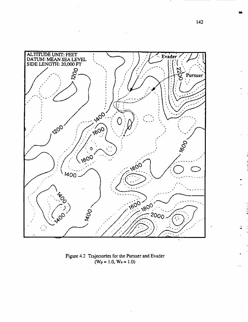
142
I
.... _% " " " # I I j . i i , • / 1_IlI_E_II.FEET _ , _ ,/.-., _.,.ao.. /, / /,
Sn_EZ_NGTrt:20,000_ "-. _ ,'/.,'/_"" i:i:/ ;, .-":-./ o , f ,.///..."-",,I,t_;,,, ,
s-- _ I I i l f I
/, ", _ _ I I , iv 'v', P_ ;_" Pursuer! ," , _ _ ! , I I"I _ _lli,u' ,
/ 1 I 1 .
I ! # /i _ f #i
¢ ...,, .'/ /t I , / // "-.I !l,V._.--_.-_• , _) . I _ .... _ ',l:t',___...
.. / .... ._,_ , N',M', 't._; ',. ,-.-----,.- -.," ,.,0 "" t,,1 ..\ , .' J(I ,, \ t /
,, ._m_, :'f.;S_o_,) '..,,'/y.' .,' '...,/-/ , !,;/_ .,( .,.. ,.. ./
,'l,'l" -, _ , , 0. /,1 .... \ , , _)
I _ .."/.,/ '._ i .."_..- .--" _ .,-'/ ,"L"L°,e°.'-'" - -k " . ..,o / ......
• 400
/ ; .-. _ ; /',_.-" ,--.
"X.-,) J "' .......i # _ _ _ _l_ _#
',.\ ', V° .---o,,,_, ...----...>D X "7._@'-,_@--"--;J-">,_\ ::(oo" 2 ;>_ /,..-/.-__A;2oo ,
__,_ ,/..,/>"../._', iW_)./..-'" ,-' --J ."/-'/9"_':}" -,-..'_-X..'"_ ¢ - ,-" • / .t __4
l
Figure 4.2 Trajectories for the Pursuer and Evader
GVp = 1.0, W_ = 1.0)

143
v
e.3
_.="/=IM
<
2400[
Pursuer /I
_°°f .........._va,o, /__ooo[- //-
;"
1800
1600
1400 " ' ' ' ' ' ' ' ' '0 20 40 60 80
Time-to-Go (sec)
i
100
Figure 4.3 Altitude Histories for the Pursuer and Evader

I
144
Figure 4.4 Trajectories for the Pursuer and Evader(Wp = 1.0, Wc = 1.0)

145
V
o
2m
<
20OO
1800
1600
1400
12000
= I = I = I = I
2O 40 6O 80
Pursuer
Evader
100
Time-to-Go (see)
Figure 4.5 Altitude Histories for the Pui'suer and Evader

146
/
Pursuer#
J
=
v
Figure 4.6 Trajectories for the Pursuer and Evader
(Wp = 0.0, We = 1.0)
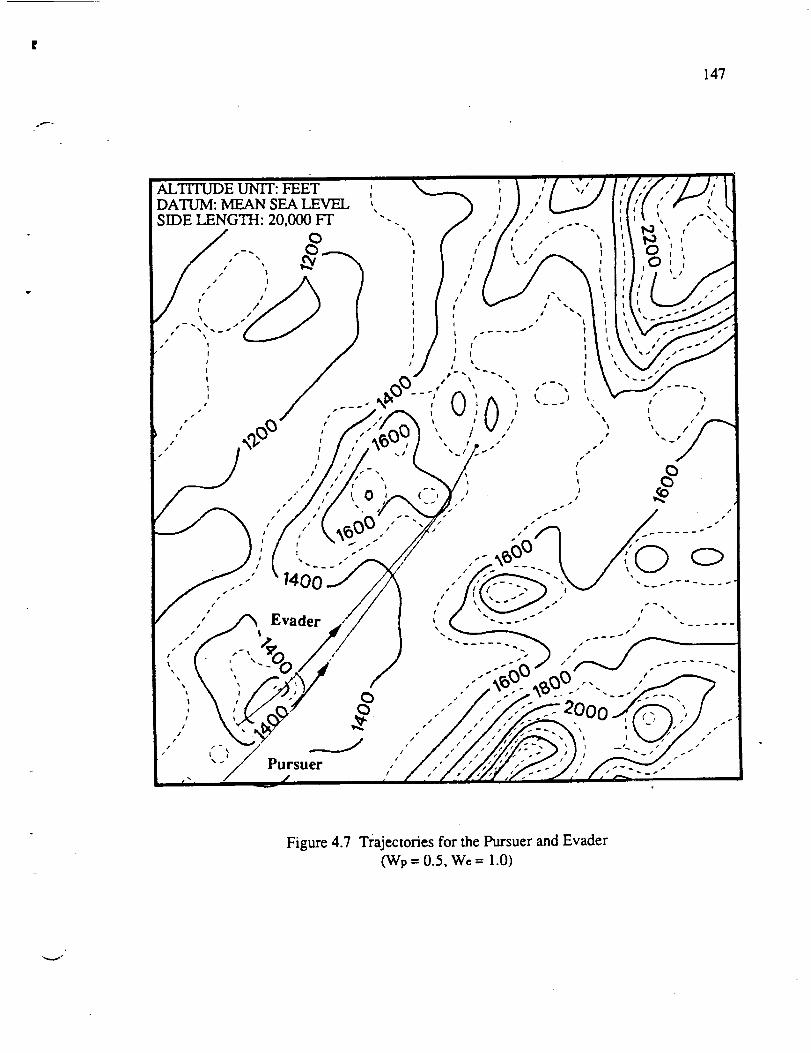
147
ALTITUDE UNIT: FEETDATUM: MEANSEALEVEL
SIDE LENGTH: 20,000 FT
/
Figure 4.7 Trajectories for the Pursuer and Evader
(Wp = 0.5, We = 1.0)

148
1000
0
-10000
Pursuer
.......... Evader
• I _ I i I i i
20 40 60 80 100
w
Time-to-Go (see)
Figure 4.8 Legendre-Clebsch Test for the Pursuer and Evader
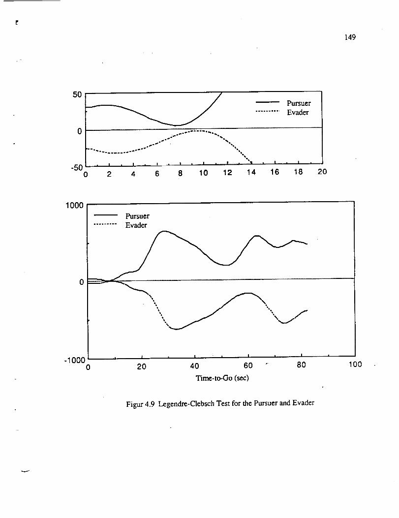
149
50
0
-500
,,,. w "p gj,o"* "%* % "%'_'_e,
• I I , I L, I • I • I , q'qll
2 4 6 8 10 12 14 16
Pursuer
Evader
I
18
|
20
1000
Pursuer.......... Evader
0
-10000
i ( i f i I , f
20 40 60 " 80
Time-to-Go (sec)
IO0
Figur 4.9 Legendre-Clebsch Test for the Pursuer and Evader
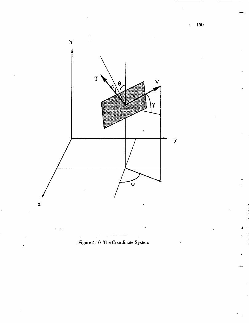
m
150
X
h
T
Y
Figure 4.10 The Coordinate System
v
.t
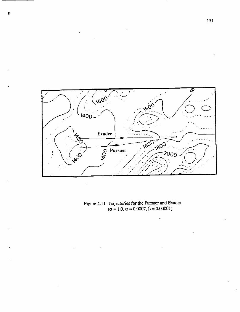
151
".; ,, /..,,," , v ,:_,. i " ,",..-" ,f'_ . ..../ . :/ . ',.., ..- ,. ,'
.," X " " ' rL "'_ " " "" / "\ / " , _k,) .. .- ," ,.-,P'_ x ...... -"
/-:.- _o_.- , ./_- ....:_-:,..., .__.-......." , ., ! . .-.' .'-_---':-- ;" '-.
l il -, ____ .., _-_______.j_ _-___-__ _--,___ .........",,, ' _A__..+4_. _ ---- ..-,,_)0 0,0{3 ..... " /-_.,_"\ _/ "':./ 0 Pursuer ,./_.,_.yO_ :- .. :S. (,'\ ( ,,0 o . /' ."/'.;-";:_00,',...-,'-'--IX, ..b,_ _ .,, ,..-./.__ _, ,(..) / ..xL.x ., .- ./.-/.,,';,:_--'._',;..d/..-
/; ,_---" . ," • ...":_'/i'::L: ) : i : -'-._..," ,- "- / ,; ,,:...:,.;//.7./._.:-:>._...
Figure 4.11 Trajectories for the Pursuer and Evader
(o = 1.0, (x = 0.0007, 13= 0.00001)

152
8
v
O'2
180
170
160
150
140
1300
Pursuer
Evader
20 40 60
Time (sec)
8O
W
J
z
Figure 4.12 Speed Histories for the Pursuer and Evader

153
2
0 I I I
0 20 40 60
Vl._sLlel" ]
Evader
I & I I
8O
Time (sec) --
Figure 4.13 Load Factor Histories for the Pursuer and Evader

154
<
2o
lO
o0
Pursuer
Evader
20 40 60 80
Time (sec)
Figure 4.14 Bank Angle Histories for the Pursuer and Evader
2.
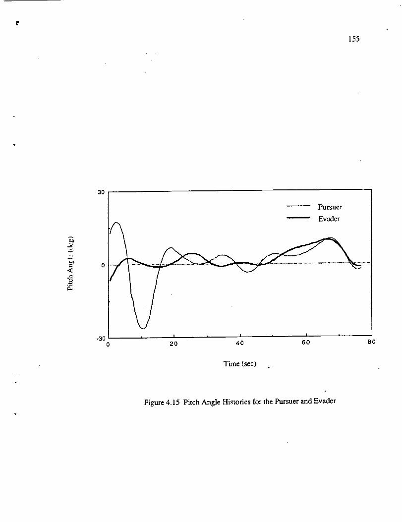
155
e-<
3o
-300
| ! I i
2O 40 60
Pursuer
Evader
8O
Time (sec)
Figure 4.15 Pitch Angle Histories for the Pursuer and Evader

156
2
<
1800
1700
1600
1500
1400
1300
12000
"-- Pursuer
Evader
I
20
I
60 80
Time (sac)
Figure 4.16 Altitude Histories for The Pursuer and Evader
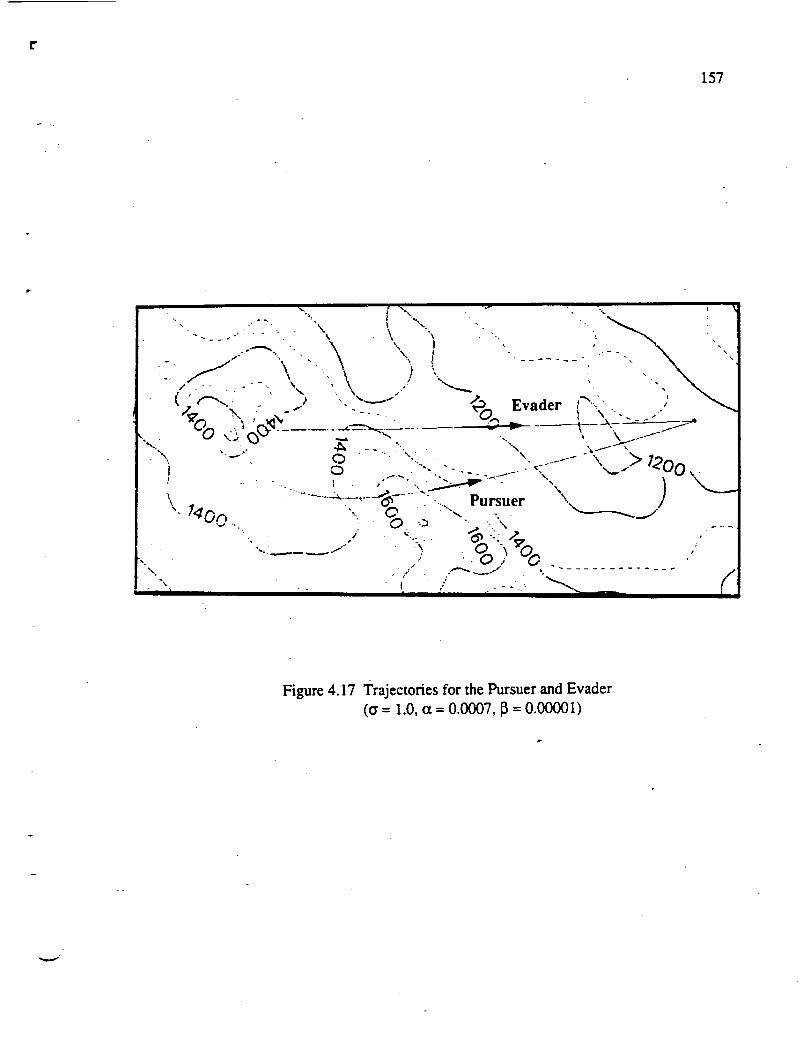
[-
157
Figure 4.17 Trajectories for the Pursuer and Evader
(a = 1.0, et = 0.0007, p = 0.00001)
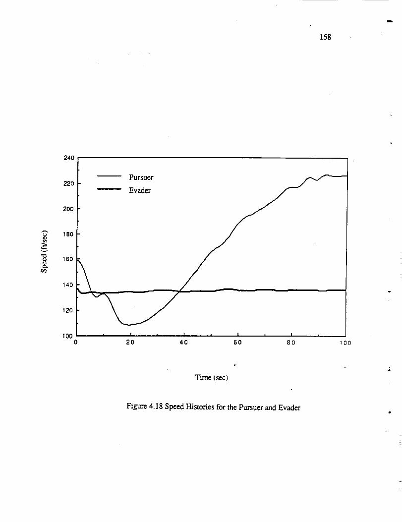
158
240
220
200
180
160
140
120
IO00
Pursuer
Evader
20 40 60 80 100
Time (sec)
,L
Figure 4.18 Speed Histories for the Pursuer and Evader
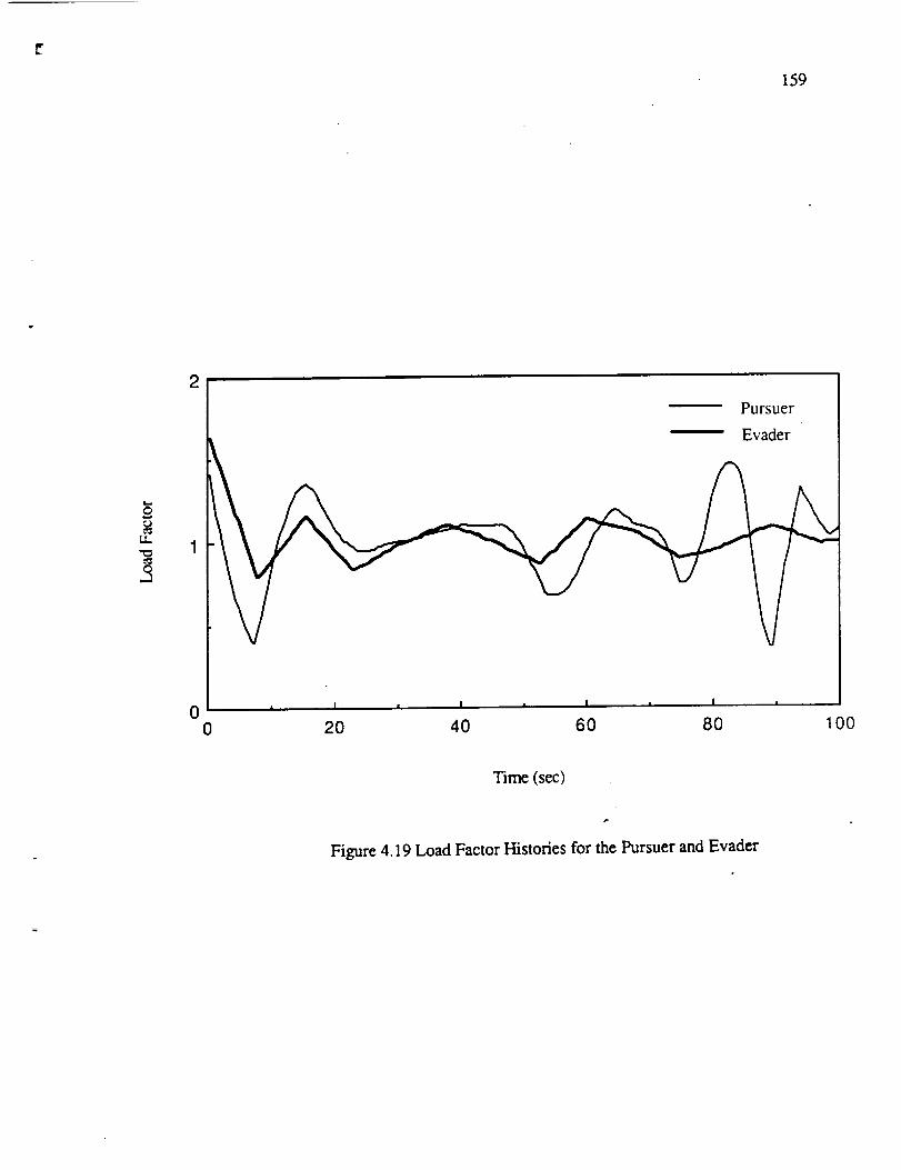
159
rz_
2
0 I =
0 20 40 60 80
Pursuer
Evader
100
Time (sec)
Figure 4.19 Load Factor Histories for the Pursuer and Evader

k
160
3O
¢J5
g,)
<
,--j
2O
10
0
0
Pursuer
Evader
20 40 60 80 1(X)
Time (sec)
Figure 4.20 Roll Attitude Histories for the Pursuer and Evader

161
ed_
m
</-
°_
3O
-30
0
Pursuer
Evader
20 40 60 80 1 O0
Time (sec)
w
Figure 4.21 Pitch Attitude Histories fot the Pursuer and Evader

162
L_
°_
<
1800
1600
1400
1200
10000
Pursuer
Evader
20 40 60 80 100
Time (sec)
Figure 4.22 Altitude Histories for The Pursuer and Evader
qll

163
40
20
..400 20 40 60 80
Time (sec)
100
Figure 5.1 Rate of Climb for Maximum Terrain Masking Trajectory
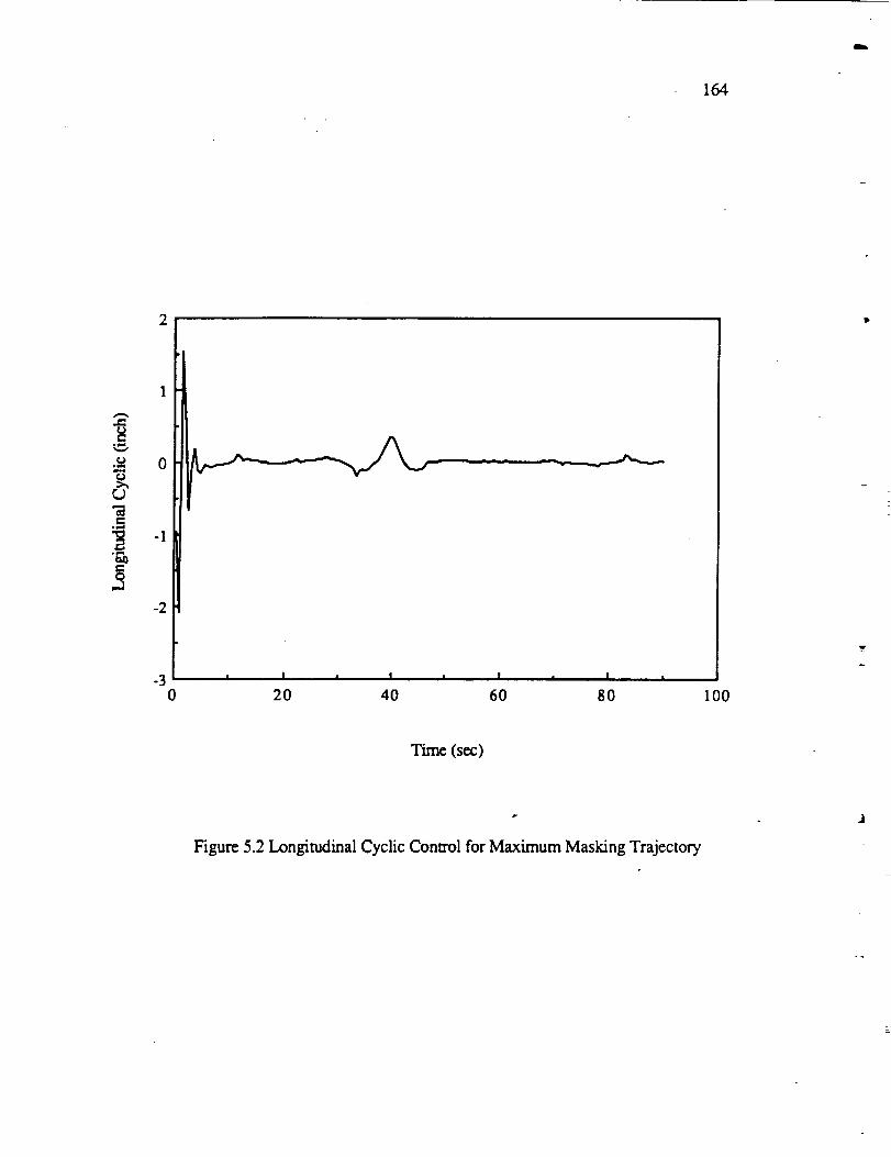
164
h
2
1
-2
._ I I I I I I I I I
0 20 40 60 80 100
Time (se,c)
Figure 5.2 Longitudinal Cyclic Control for Maximum Masking Trajectory

165
0.1
°q,u
, 0.0
-0.1 j I f I , I i I
0 20 40 60 80
Time (sec)
Figure 5.3 Lateral Cyclic Control for Maximum Masking Trajectory
I00
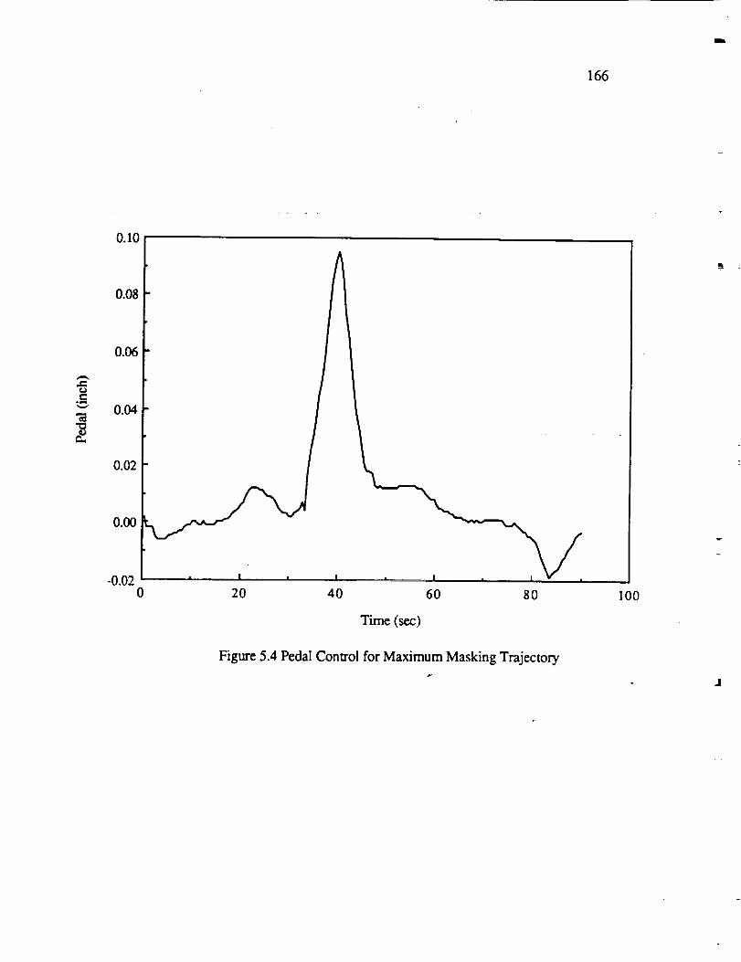
166
e,.
0_I0
0.08
0.06
0.04
0.020.00
-0.02 , I ,0 20 40 60 80
Time (sex:)
Figure 5.4 Pedal Control for Maximum Masking Trajectory
I00

167
_d
80
60
40
20 I _ I , I , I
20 40 60 80
Time (sec)
100
Figure 5.5 Collective Control for Maximum Masking Trajectory

168
4
0
<
-2
..4
0 20 40 60 80
Time (sec)
100
Figure 5.6 Pitch Attitude Response for Maximum/v_sking Trajectory1
-r

169
20
10
m
<
0
-|0 I I i , I i t i I
0 20 40 60 80
Time (sec)
100
Figure 5.7 Roll Attitude Response for Maximum Masking Trajectory
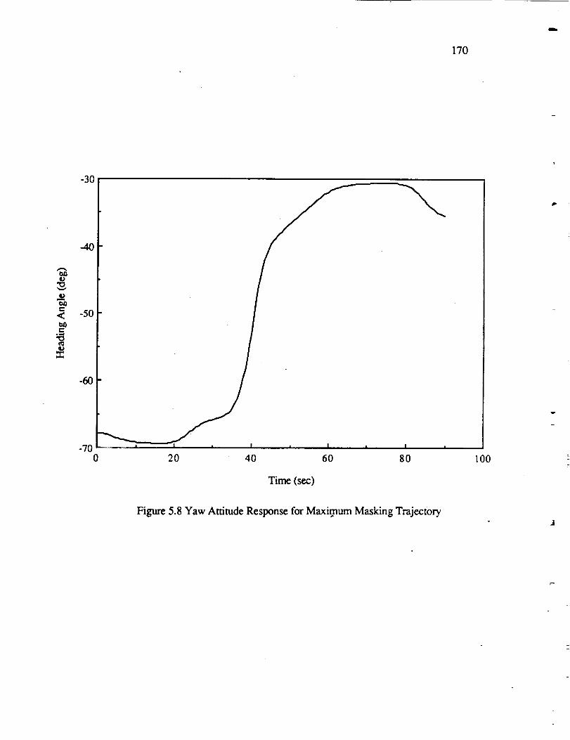
170
o=
<
e-
t_
-30
-40
-50
-60
-700
m
20 40 60
! • m
80
Time (sec)
100
P
Figure 5.8 Yaw Attitude Response for Maximum Masking Trajectory

[..
172
2
,,c
C..)m
t,,,,,,
o!
20 40 60 80
Time (sec)
Figure 5.10 Longitudinal Cyclic Control for Minimum Time Trajectory
00

173
0.2
,J=¢.)e-
°¢-w
ow.i
..1
0.1
0.o
-0.1 i I i I i I i I
20 40 60 80J
lOO
Time (sec)
Figure 5.11 Lateral Cyclic Control for Minimum Time Trajectoryw-
.1
L •

174
w..
0.04
0.02
0.00
-0.02
-0.04
-0.06 ! I _ I = I
20 40 60 80
Time (see)
!
100
Figure 5.12 Pedal Control for Minimum Time Trajectory

175
¢)
.=>
9O
80
7O
6O
5O
4O
3O
200 20 40 60 80 100
e
v
Time (sec)
Figure 5. 13 Collective Control for Minimum Time Trajectory
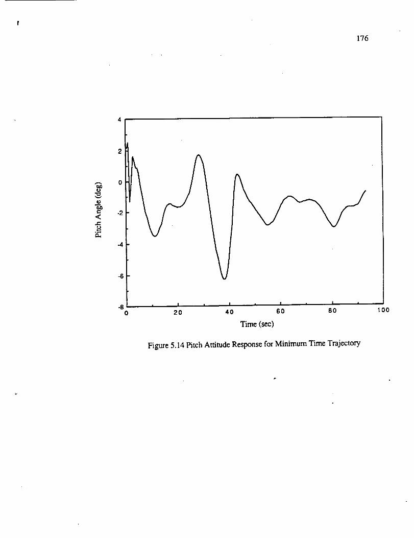
176
4
o
o
c<..1=
20 40, I
6O
Time (see)
/
i I i
8O
Figure 5.14 Pitch Attitude Response for Minimum Time Trajectory
00

177
o
o
<
e_
0
! _ I
20 40 60 80
_me(s_)
100
v
Figure 5.15 Roll Attitude Response for Minimum Time Trajectory

171
e-,
E
L_
0
C_
4O
20
-60o 20 40 60 80 100
Time (sec)
Figure 5.9 Rate of Climb for Minimum Time Trajectory

tm
qo
tut_t-
<I:mC
o_
-40
-50
-600 20 4O 60 80 100
Time(sec)
P
Figure 5.16 Yaw Attitude Response for Minimum Time Trajectory

Form Approved
REPORT DOCUMENTATION PAGE oM8No.o7o4-o188
Public reporting burden for this collection of information is estimated to average I hour per response, including the time for reviewing instructions, searching existing data sources,
! gathering and maintaining the data needed, and completing and reviewing the collection of information. Send comments regarding this burden estimate or any other aspect of this
collection of information, including suggestlons for reducing this burden, to Washington Headquarters Services, Directorate for information Operations and Reports, 1215 Jefferson
Davis Highway.Suite 1204, Arlington,VA 22202-4302. and to the Office of Management and Budget, PaperworkReductionPro act (0704-0188). Washington, DC 20503.
1. AGENCY USE ONLY (Leave blank) 2. REPORT DATE 3. REPORT TYPE AND DATES COVERED
March 1990 Contractor Report4. TITLE AND SUBTITLE 5. FUNDING NUMBERS
Optimal Helicopter Trajectory Planning for Terrain Following Flight
6. AUTHOR(S)
P. K. A. Menon and E. Kim
7. PERFORMING ORGANIZATION NAME(S) AND ADDRESS(ES)
Georgia Institute of Technology
School of Aerospace Egnineering
Atlanta, GA 30332
9. SPONSORING/MONITORING AGENCY NAME(S) AND ADDRESS(ES)
Ames Research Center
Moffett Field, CA 94035-1000
NAG2-463
8. PERFORMING ORGANIZATIONREPORT NUMBER
A-93060
10. SPONSORING/MONITORINGAGENCY REPORT NUMBER
NASA CR-177607
11. SUPPLEMENTARY NOTES
Point of Contact: Victor H. L. Cheng, Ames Research Center, MS 210-9, Moffett Field, CA 94035-1000;(415) 604-5424
12a. DISTRIBUTION/AVAILABILITY STATEMENT
Unclassified -- Unlimited
Subject Category 04
12b. DISTRIBUTION CODE
13. ABSTRACT (Maximum 200 words)
Helicopters operating in high threat areas have to fly close to the earth surface to minimize the risk of being detected
by the adversaries. This report presents techniques for low altitude helicopter trajectory planning. These methods are
based on optimal control theory and appear to be implementable onboard in realtime. Second order necessary
conditions are obtained to provide a criterion for finding the optimal trajectory when more than one extremal passes
through a given point. A second trajectory planning method incorporating a quadratic performance index is also
discussed. In a later part of the thesis, trajectory planning problem is formulated as a differential game. The objective
here is to synthesize optimal trajectories in the presence of an actively maneuvering adversary. Numerical methods
for obtaining solutions to these problems are outlined. As an alternative to numerical method, feedback linearizing
transformations are combined with the linear quadratic game results to synthesize explicit nonlinear feedback
strategies for helicopter pursuit-evasion. Some of the trajectories generated from this research are evaluated on a six-
degree-of-freedom helicopter simulation incorporating an advanced autopilot. The optimal trajectory planning
methods presented here are also useful for autonomous land vehicle guidance.
14. SUBJECT TERMS
Terrain following, Optimal control, 2nd order necessary conditions
17. SECURITY CLASSIFICATION 18. SECURITY CLASSIFICATIONOF REPORT OF THIS PAGE
Unclassified Unclassified
NSN 7.540-01-280-5500
19. SECURITY CLASSIFICATIONOF ABSTRACT
15. NUMBER OF PAGES
18016. PRICE CODE
A09
20. LIMITATION OF ABSTRACT
Standard Form 298 (Rev. 2-89)Prescribed by ANSI Std, Z39-18

,.&