Optimal Generic Advertising under Bilateral Imperfect Competition between Processors and Retailers

Chanjin Chung, Young Sook Eom, Byung Woo Yang, and Sungill Han

Selected paper prepared for presentation at the Agricultural and Applied Economics Association’s 2013 AAEA & CAES Joint Annual Meeting, Washington D.C., August 4-6, 2013. Copyright 2013 by Chanjin Chung, Young Sook Eom, Byung Woo Yang, and Sungill Han. All rights reserved. Readers may make verbatim copies of this document for non-commercial purposes by any means, provided that this copy right notice appears on all such copies. Chanjin Chung is professor and Breedlove Professor at Oklahoma State University, Young Sook Eom and Byung Woo Yang are professors at Chon-buk National University, Korea, and Sungill Han is professor at Konkuk University, Korea. This research was supported by the Oklahoma State University Agricultural Experiment Station.

2

Optimal Generic Advertising under Bilateral Imperfect Competition between Processors and Retailers

Abstract

The purpose of this paper is to examine the impact of bilateral imperfect competition

between processors and retailers and of import supply on optimal advertising intensity,

advertising expenditures, and checkoff assessment rates. First, comparative static

analyses were conducted on the newly developed optimal advertising intensity formula.

Second, to consider the endogenous nature of optimal advertising, a linear market

equilibrium model was developed and applied to the U.S. beef industry. Results showed

that the full consideration of retailer-processor bilateral market power lowered the

optimal values of assessment rates, advertising expenditures, and advertising intensity for

the checkoff board while consideration of importers increases the optimal values. The

results indicate that ignoring the import sector in optimal generic advertising modeling

should underestimate these optimal values, while ignoring the bilateral market power

between processors and retailers overestimates the values.

Key words: bilateral market power, checkoff, import supply, oligopoly, oligopsony,

optimal advertising, processor, retailer

[EconLit citations: L13, L66, M37]

3

Agricultural producers have invested over $750 million annually into self-financed

“checkoff” programs designed to increase their profits for various commodities. These

checkoff programs have a long history dating back to the late 1800s with the creation of

state-level voluntary programs to promote farm commodities. Since the mid-1980s,

many state-level checkoff programs have been expanded to federally-legislated

mandatory programs. These mandated programs require producers to pay a specified

amount of money through either per unit or value assessment. For example, the dairy

checkoff program that funds the well-known advertising campaign, “got milk” mandates

all dairy farmers to pay fifteen cents per hundredweight of all milk marketed. The pork

program that sponsors the “Pork: the Other White Meat” campaign specifies a mandatory

assessment rate of 0.40 percent of sales value.

The specified checkoff assessment rates raise several important questions,

particularly related to how they are determined and whether they can generate profit-

maximizing advertising expenditures. Some producer groups are concerned that the

current assessment is too small to produce significant advertising effects for their industry

and is probably not profit maximizing. For example, in the summer of 2006, a task force

team co-chaired by the National Cattlemen’s Beef Association and the American Farm

Bureau Federation evaluated the beef checkoff program and recommended an adjustment

of the checkoff rate from the current one dollar to two dollars per head (Farm Futures,

2006). The committee recognized that the total beef chcekoff collection has been

continuously declining, and as a result, the advertising expenditures have also been

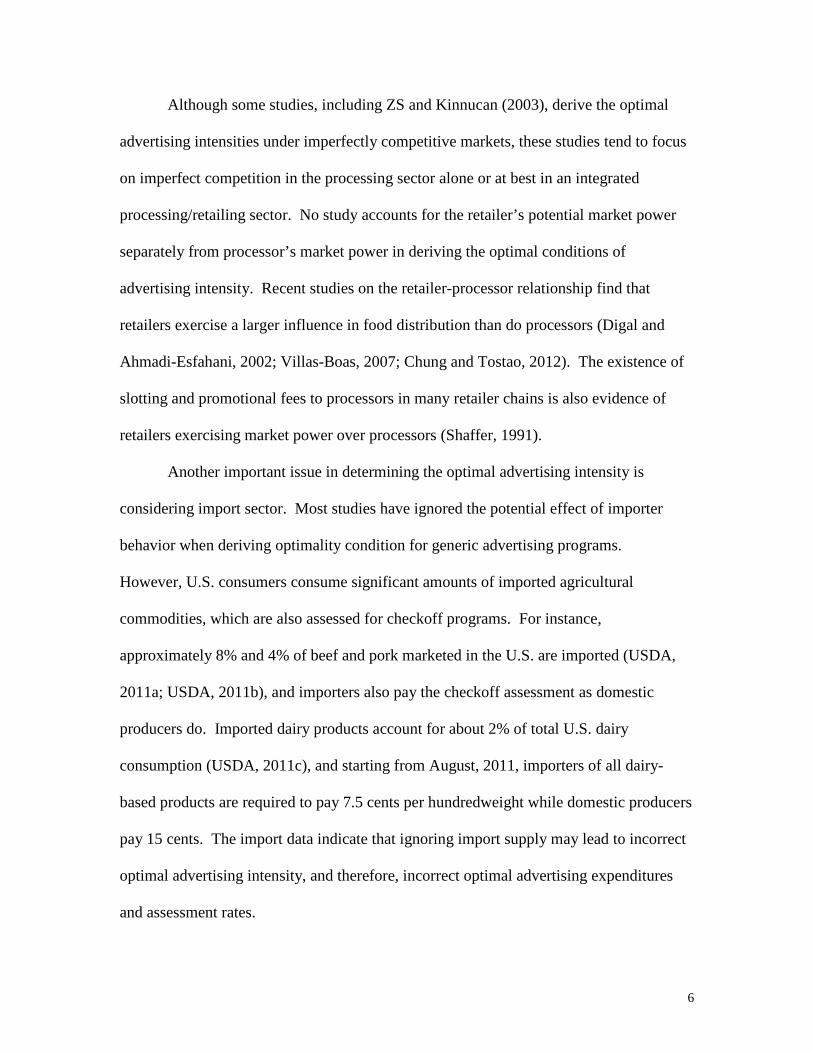
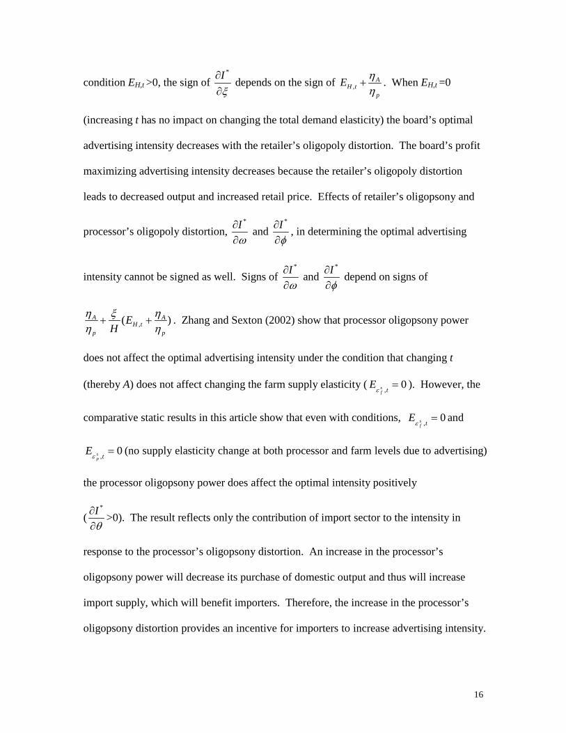
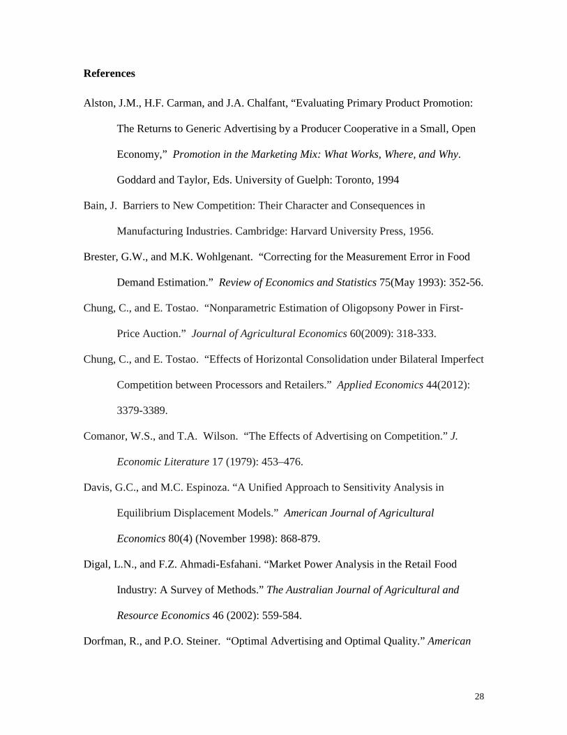
declining. In fact, the advertising expenditure for the beef industry peaked in 1990 at 33

million dollars, but since then, it has been continuously decreasing and was down to 18

4

million dollars in 2011 (Figure 1). Figure 1 also shows that the declining trend is even

more noticeable when the expenditures are deflated by Media Cost Index (MCI) and

Consumer Price Index (CPI).

Numerous studies have examined the optimality of advertising expenditures in

both economics and agricultural economics literature (Dorfman and Steiner, 1954;

Nerlove and Waugh, 1961; Goddard and McCutcheon, 1993; Zhang and Sexton, 2002;

Kinnucan, 2003). One central issue in these studies is to determine the condition of

optimal advertising intensity. The well-known Dorfman and Steiner (DS) Theorem

(1954) shows that the optimality condition for joint price and advertising expenditure is

characterized by the equality of the ratio of advertising (A) to sales (PQ), (where P and Q

represent sales price and quantity, respectively) with the ratio of the advertising elasticity

( Aη ) to the absolute value of price elasticity of demand ( || Pη ), i.e., PQA

P

A =||η

η .

Goddard and McCutcheon (GM) (1993) follow a similar framework to DS but allow both

price and quantity to vary in response to the effective advertising. GM show that optimal

advertising conditions are the same whether quantity is assumed fixed or whether both

quantity and price are allowed to adjust to advertising. Unlike the previous two studies,

Nerlove and Waugh (NW) (1961) assume that producers have alternatives for the use of

collected funds spent on advertising. In previous studies, the first order condition for the

producer’s profit maximization condition with respect to advertising equals zero.

However, recognizing alternative uses of these funds such as buying government bonds,

NW equate the marginal returns to the rate of returns on alternative forms of investment

(ρ). NW also assume the supply response to advertising. Then, the corresponding

5

optimal advertising condition becomes ( )(1 )

A

P

APQ

ηε η ρ

=− +

, where ε is the supply

elasticity. Including the three studies reviewed so far, most studies in generic advertising

literature derive the optimality condition under the competitive market structure.

However in recent years, as food processing and retailing sectors have become

increasingly concentrated, several studies have found the existence of imperfect

competition in these sectors (Paul, 2001; Lopez, Azzam, and Espana, 2002; Chung and

Tostao, 2009; Chung and Tostao, 2012).

To reflect the change in market structure in food processing and retailing sectors,

Zhang and Sexton (ZS) (2002) and Kinnucan (2003) consider imperfect competition in

deriving the optimality condition of advertising. ZS investigate the optimal conditions of

generic advertising for agricultural markets where the downstream market exhibits

oligopoly and oligopsony power. The optimal condition derived by ZS shows that unless

advertising makes the demand more elastic, downstream oligopoly power reduces the

optimal advertising intensity below the level specified by DS. Simulation results show

that the producer checkoff rate increases as a function of the degree of oligopoly power in

the downstream market while it decreases under its oligopsony power or joint oligopoly

and oligopsony power. Kinnucan (2003) also investigates the impact of food industry

market power on producers’ optimal advertising level, but focuses on the assumption of

technology for the food processing industry. His study assumes that food industry

technology is characterized by variable proportions while possessing market power.

Kinnucan concludes that market power tends to reduce the optimal level of advertising,

but the reduction is moderated by factor substitution.

6

Although some studies, including ZS and Kinnucan (2003), derive the optimal

advertising intensities under imperfectly competitive markets, these studies tend to focus

on imperfect competition in the processing sector alone or at best in an integrated

processing/retailing sector. No study accounts for the retailer’s potential market power

separately from processor’s market power in deriving the optimal conditions of

advertising intensity. Recent studies on the retailer-processor relationship find that

retailers exercise a larger influence in food distribution than do processors (Digal and

Ahmadi-Esfahani, 2002; Villas-Boas, 2007; Chung and Tostao, 2012). The existence of

slotting and promotional fees to processors in many retailer chains is also evidence of

retailers exercising market power over processors (Shaffer, 1991).

Another important issue in determining the optimal advertising intensity is

considering import sector. Most studies have ignored the potential effect of importer

behavior when deriving optimality condition for generic advertising programs.

However, U.S. consumers consume significant amounts of imported agricultural

commodities, which are also assessed for checkoff programs. For instance,

approximately 8% and 4% of beef and pork marketed in the U.S. are imported (USDA,

2011a; USDA, 2011b), and importers also pay the checkoff assessment as domestic

producers do. Imported dairy products account for about 2% of total U.S. dairy

consumption (USDA, 2011c), and starting from August, 2011, importers of all dairy-

based products are required to pay 7.5 cents per hundredweight while domestic producers

pay 15 cents. The import data indicate that ignoring import supply may lead to incorrect

optimal advertising intensity, and therefore, incorrect optimal advertising expenditures

and assessment rates.

7

Objectives of this study are to derive an optimal advertising intensity formula that

considers bilateral imperfect competition between processors and retailers and the supply

of imported goods and to examine the impact of these unique features of derivation on

optimal advertising intensity, advertising expenditures, and checkoff assessment rates.

Unlike many previous studies, we model retailing and processing sectors separately and

consider the processors’ interaction effect with retailers in deriving the optimal

advertising rule. Our approach relies on market equilibrium conditions and a combined

pricing rule derived from first-order conditions of two separate profit maximization

problems for a retailer and a processor and thus takes into account both upstream and

downstream competitions in retail and processing sectors. For most checkoff programs,

boards make decisions on the level of advertising expenditures based on estimated funds

to be collected, but effective advertising programs induce changes in industry sales which

affect the collected checkoff funds and, in turn, the money available for advertising.

Therefore in this case, the advertising expenditures are endogenously determined by

market equilibrium (Kinnucan and Myrland, 2000; Zhang and Sexton, 2002). The

market equilibrium conditions of our approach include the endogenous nature in

determining optimal advertising expenditures. To further illustrate the impact of bilateral

market power (between processors and retailers) and importer behavior on the optimal

level of advertising expenditures, we also develop a market equilibrium model that

consists of retail demand, processor and import supply, and farm supply functions. The

market equilibrium model is simulated with various levels of market power parameters,

holding all other market parameters constant. The model is also applied to the U.S. beef

industry to obtain optimal advertising intensity, advertising expenditure, and assessment

8

rate, and the results are compared to previous approaches that do not consider bilateral

imperfect competition and import sector. Monte Carlo simulations are conducted to

construct confidence intervals for sensitivity analyses of the results and comparisons of

their mean differences.

Derivation of Optimal Advertising Intensity

In deriving the optimal advertising intensity, we extend previous studies, in particular,

Zhang and Sexton (2002) and Kinnucan (2003), in two ways. First, we develop a model

that allows retailer’s oligopoly and oligopsony power separately from processor’s market

power. To allow the market power at retail and processing sectors separately, retailer and

processor profit maximization problems are solved sequentially, and the profit

maximization conditions are incorporated in a multi-equation model. Secondly, the new

framework also considers import effects in determining optimal generic advertising

intensity. To consider the import effects in our derivation, we include the import supply

equation and the identity condition that equates retail demand with domestic supply plus

import supply.

Therefore, our new framework includes equilibrium conditions of each production

stage with consideration of trade and potential bilateral market power from retailers and

processors. Our approach first defines a set of market equilibrium conditions and derives

marginal effects of a change in assessment rate on equilibrium prices and quantities.

Then, the optimal advertising intensity is determined from the derived marginal effects

using the condition of checkoff board surplus maximization.

Consider a three-sector model where retailing and processing sectors are

imperfectly competitive in both raw material and output markets, and the farm sector is

9

perfectly competitive in the output market. In this framework, retailers and processors

exercise oligopsony power when procuring their raw materials while they also exercise

oligopoly power in selling their products. Let md YYY += , where Y is the aggregate

quantity available at retail level, Yd is domestic production, and Ym is the quantity

imported. Assuming constant return to scale in the food processing technology and fixed

proportions with Leontief coefficient 1 in converting from farm to retail products leads to

fpd YYY == , where Yp and Yf are aggregate product quantities at processing and farm

level, respectively.1 We also define the advertising expenditure (A) as: tYA = , assuming

all collected money is utilized for advertising, and t is the per-unit tax on domestic

production and imports. Then, when pr , pp , and pf are prices at retail, processing, and

farm level, the market equilibrium can be expressed as the following set of equations:

(1) )](,[ tAPDY r= , retail demand,

(2) ),( tPSY fdd = , domestic supply,

(3) ),( tPSY rmm = , import supply,

(4) md YYY += , identity condition,

(5) A = tY(Yd , Ym), advertising expenditure.

Considering nr identical retailers, i.e., Y = nryr, we have a representative retailer’s

profit maximization problem as:

rps

prr

yymYPytYPMax

r])([),( +−=π ,

where yr and m represent finished product sales and constant marketing cost per unit for

the representative retailer, respectively. The first order condition to the retailer’s problem

with respect to yr leads to:

10

(6) ,)1)(()),(

1)(,( mYPtYH

tYP sp

ppr ++=+εωξ

where )/)(/( YyyY rr∂∂=ξ and )/)(/( prrp YyyY ∂∂=ω are conjectural elasticities

reflecting the degree of competition among retailers in selling finished products (ξ) and

procuring processed products (ω), respectively;

)1/()/)(/(),( APrr YPdPdYtYH ηη −== and )/)(/( p

sppp

ssp YPdPdY=ε are total price

elasticity of demand and elasticity of processor supply, respectively.

Considering np identical processors, i.e., YP = npyp, a representative processors’

profit maximization problem is:

pfPppd

p

yyctYWyYPMax

p]),([)( +−=π ,

where yp and c represent processed product sales to retailers and the constant processing

cost per unit for the representative processor, respectively; and WP is the price paid by

processors to producers, and the relationship between WP and Pf is represented by

tPW fp += . The first order condition of the processor’s problem can be written in

elasticity form as:

(7) ,)1)(,()1)(,( cttYPtYP sf

ffdp

pp +++=+εθ

εφ

where the conjectural elasticity, )/)(/( pppp YyyY ∂∂=φ and )/)(/( fppf YyyY ∂∂=θ

represent degree of competition among processors in selling processed products (φ ) and

procuring farm products (θ ), respectively; )/)(/( pd

pppd

dP YPdPdY=ε and

)/)(/( ffffsf YPdPdY=ε are the elasticity of derived demand at processor level and the

supply elasticity at farm level, respectively. Substituting equation (6) in equation (7)

11

results in:

(8) .)1](),()1[(/1

1)),(

1)(,( mcttYPtYH

tYP sp

ffsf

dp

r ++++++

=+εϖ

εθ

εφξ

Totally differentiating equations (1), (2), (3), (4), and (8) with respect to t results

in:

(9) )],(),([dt

dYdt

dYtYYYAD

dtdP

PD

dtdA

AD

dtdP

PD

dtdY md

mdr

r

r

r ++∂∂

+∂∂

=∂∂

+∂∂

=

(10) ,dt

dPPS

dtdY f

f

dd

∂∂

=

(11) ,dt

dPPS

dtdY r

r

mm

∂∂

=

(12) ,dt

dYdt

dYdtdY md

+=

(13) )1]()1[()()/1(

1)),(

1( 222 sp

fsf

dP

dP

dP

rr

ctPdt

ddt

dHHP

dtdP

tYH εϖ

εθε

εφ

εφξξ

+++++

−=−+

.)(

])1)[(/1

1()/1

1)(1](1)(

)1[( 22 dtd

ctPdt

dPdt

dP sp

sp

fsf

dp

dp

sp

sf

sf

ff

sf

εεϖ

εθ

εφεφεϖε

εθ

εθ

++++

−+

++−++

Equation (13) can be rewritten in elasticity form as:

)1]()1[()/1(

1

)1)(1(/1

1)),(

1(

,2 s

p

fsf

dP

tdP

f

sf

sp

dp

r

ctPt

Edt

dPdt

dPtYH

dP

εϖ

εθ

ε

φ

εφ

εθ

εϖ

εφξ

ε +++++

−=

+++

−+

,

])1)[(/1

1()/1

1)(1)](1(

,

,,

tH

r

tsp

fsf

dp

dp

sp

tsf

f

EHtP

Et

ctPEtP

sP

sf

ξ

εϖ

εθ

εφεφεϖ

εθ

εε

+

++++

−+

++−+

where ,, dp

dp

t

tdt

dE d

P εε

ε= ,, s

p

sp

t

tdt

dE s

P εε

ε= and

sf

sf

t

tdt

dE s

f εε

ε=, . ,,td

pEε

,,tsp

Eε

and tsf

E ,ε

(13′)

12

represent the percentage change in elasticities of processors’ derived demand and supply,

and the elasticity of farm supply in response to one percent change in checkoff

assessment rate t, respectively. EH,t represents the percentage change in total demand

elasticity H in response to one percent change in advertising assessment t.

Equations (9), (10), (11), (12), and (13′) can be rewritten in matrix form as:

(14)

+

++−+

−−∂∂

−

∂∂

−

∂∂

−∂∂

−∂∂

−

dtdPdt

dYdt

dYdt

dPdtdY

H

PS

PS

ADt

ADt

PD

f

m

d

r

dp

sf

sp

r

m

f

d

εφεθ

εϖ

ξ/1

)1)(1(0010

01101

0100

0100

01

= ,

000

Ω

∂∂ Y

AD

where

)1]()1[()/1(

1 ,2 s

P

fsf

dp

tdp

ctPtE d

P

εϖ

εθ

ε

φ

εφε ++++

+−=Ω

.])1)[(/1

1()/1

1)(1)(1( ,,, tH

r

tsp

fsf

dp

dp

sp

tsf

f

EHtPE

tctPE

tP

sp

sf

ξεϖ

εθ

εφεφεϖ

εθ

εε++++

+−

+++−+

In previous studies (Alston, Carman, and Chalfant, 1994; Zhang and Sexton,

2002), a producer group’s surplus maximization problem is considered to decide the per-

unit assessment rate (t), and consequently generic advertising expenditures (A) for

deriving an optimal generic advertising rule. The previous derivations do not take into

account importer’s surplus maximization. However, many commodity checkoff boards

include importers as their members and therefore need to also consider importers’

benefits when deciding the optimal per unit assessment rate (t). To account for both

13

domestic producer’s and importer’s surplus maximizations, we derive an optimal

assessment condition from the first-order-condition of a combined producer-importer

surplus maximization problem as:

(15) .0***

=∂

∂+

∂∂

=∂∂

tY

tY

tY md

Equation (15) suggests that the optimal assessment can be determined when the

combined equilibrium quantity no longer changes even if the assessment rate changes.

Applying the optimality condition, equation (15), to matrix (14), we have:

(16) ,0

1

11

1

1=

∂∂

∂∂

+

+

+

+∂∂∂∂Ω

−∂∂

Ω+

∂∂

∂∂

Ω+∂∂

++

∂∂

Ω−∂∂∂∂

Ω

Ψr

m

dp

sf

sp

f

d

f

d

f

d

rr

m

r

m

PSY

AD

APSDt

PS

PS

PDY

AD

HPS

PASDt

εφ

εθ

εϖ

ξ

where

.111

11

∂∂

−

+

∂∂

+

∂∂

−∂∂∂∂

−∂∂

+

+

+

=ΨADt

HPS

PD

PASDt

PS

f

d

rr

m

r

m

dp

sf

sp ξ

εφ

εθ

εϖ

Rewriting equation (16) in an elasticity form and rearranging it results in the optimal

advertising intensity (I*) as:

(17)

−

+−

+

+

−

+−== 2,

***

*

)1(1

1

11

τεθ

εητηη

εϖ

εφ

ξξηη f

sf

sfp

mA

sp

dp

tHp

Ar

fEHH

IYP

A,

14

where m r

m r mS PP S

η ∂=∂

is the import supply elasticity,mS

Yτ = is the import share from total

consumption, and ff is the producer share from total retailer revenue, i.e.,

r

f

r

fff

PP

YPYPf )1( τ−== .2

Equation (17) shows that the optimal advertising intensity (advertising to retailer

sales ratio) now depends on not only advertising and demand elasticities of retailers, but

also retailers’ and processors’ bilateral market power parameters, demand and supply

elasticities of processors, elasticity of farm supply, and import supply elasticity. Unlike

previous studies, the newly derived advertising intensity equation clearly shows that the

bilateral market power relationship between processors and retailers (both oligopoly and

oligopsony powers of retailers and processors) plays an important role in determining the

optimal advertising intensity when the processing sector is considered separately from a

combined processing-retailing sector. The advertising intensity derived by Zhang and

Sexton (2002) shows no direct effect of oligopsony power from the retailer-processing

sector. However, when the processing sector is considered separately from the retailing

sector, and import sector is added to the model, all four bilateral market power

parameters affect the optimal condition even if no advertising effect is assumed in

changing the elasticity of processor demand and supply elasticities of farm and

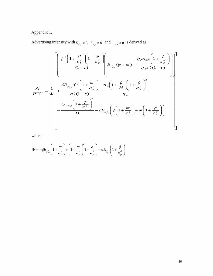
processing sectors. When the model allows advertising to change the elasticity of

processor demand and supply elasticities of farm and processing sectors, the impact of

bilateral market power between retailers and processors becomes even more extensive

(see Appendix 1). Note that equation (17) can be reduced to the Zhang and Sexton’s

optimal advertising intensity rule when an integrated retail and processing sector is

15

assumed to exert its oligopoly and oligopsony market power, and import is restricted to

zero.3 Equation (17) can be further reduced to the Dorfman and Steiner’s optimal

advertising intensity condition when no market power in retailing and processing sectors

and no import are considered.

Comparative Static Results for Optimal Advertising Intensity

Impacts of bilateral imperfect competition parameters and import supply elasticity on

advertising intensity are examined via comparative statics on equation (17). Comparative

static results are:

,01

11

,

*

<=>

+

+

+−=

∂∂

sp

dp

P

AtHE

HI

εϖ

εφ

ηη

ξ

,0)()(2,

*

<=>++

++=

∂∂

ϖεεφεε

ηηξ

ηη

ϖ sp

dp

dp

sp

p

AtH

p

A EH

I

,0)(,

*

<=>+

++−=

∂∂

ϖεεε

ηηξ

ηη

φ sp

dp

sp

p

AtH

p

A EH

I

,0)1()( 22

*

>−

−=∂∂

τεητηη

θ

f

sfP

mA fI

.0)1(

1 2

*

>

−

+−=

∂∂

τεθ

εητη

η

f

sf

sfP

A

m

fI

The impact of changing retailer’s oligopoly power on optimal advertising intensity, ξ∂∂ *I

,

cannot be signed in general. However, under the condition EH,t <0 (increasing t and thus

A induces higher consumer loyalty, therefore creating less elastic total demand elasticity)

the optimal advertising intensity decreases as the retailer’s oligopoly power increases.4, 5

This result can be justified because the less elastic retail demand due to advertisements

will increase oligopoly distortion, thereby providing less benefit to producers. Under the

16

condition EH,t >0, the sign of ξ∂

∂ *I depends on the sign of p

AtHE

ηη

+, . When EH,t =0

(increasing t has no impact on changing the total demand elasticity) the board’s optimal

advertising intensity decreases with the retailer’s oligopoly distortion. The board’s profit

maximizing advertising intensity decreases because the retailer’s oligopoly distortion

leads to decreased output and increased retail price. Effects of retailer’s oligopsony and

processor’s oligopoly distortion, ω∂∂ *I and

φ∂∂ *I , in determining the optimal advertising

intensity cannot be signed as well. Signs of ω∂∂ *I and

φ∂∂ *I depend on signs of

)( ,p

AtH

p

A EH η

ηξηη

++ . Zhang and Sexton (2002) show that processor oligopsony power

does not affect the optimal advertising intensity under the condition that changing t

(thereby A) does not affect changing the farm supply elasticity ( 0, =tsf

Eε

). However, the

comparative static results in this article show that even with conditions, 0, =tsf

Eε

and

0, =tsp

Eε

(no supply elasticity change at both processor and farm levels due to advertising)

the processor oligopsony power does affect the optimal intensity positively

(θ∂

∂ *I >0). The result reflects only the contribution of import sector to the intensity in

response to the processor’s oligopsony distortion. An increase in the processor’s

oligopsony power will decrease its purchase of domestic output and thus will increase

import supply, which will benefit importers. Therefore, the increase in the processor’s

oligopsony distortion provides an incentive for importers to increase advertising intensity.

17

However, overall effect of θ∂

∂ *I should depend on signs of ts

fE ,ε

and ts

pE ,ε

in a fully

extended model that does not impose the conditions, 0, =tsf

Eε

and 0, =tsp

Eε

(see

Appendix 1). The impact of import supply elasticity on the optimal advertising intensity,

m

Iη∂∂ *

, is positive. The result indicates that an increase in import supply elasticity will

incentivize importers to increase advertising expenditures, and therefore higher

advertising intensity.

Market Equilibrium Model

Many comparative statics in the previous section were not able to be signed, and the

comparative statics do not consider the fact that advertising decisions of many

commodity checkoff programs are often tied to industry sales and therefore determined

endogenously by market equilibrium. To address the limitation and better understand the

impact of bilateral market power between processors and retailers and the consideration

of import sector on the optimal level of advertising intensity, we construct a linear market

equilibrium model that includes retail demand, processor and import supply, and farm

supply functions. Therefore, it is important to note that the inferences of any results

should be limited to the case of the linear model. The model includes the following three

linear equations as:

(18) rPAaY αµ −+= , Retail demand

(19) ,mpp YYbP γβ ++= Processor and import supply

(20) ,ff YdP δ+= Farm supply,

where a, b, and d are intercept terms for each equation, and α, β, γ, δ, and μ are slope

18

coefficients of Pr, Yp, Ym, Yf, and A , respectively. In equation (18), the square root

form of the advertising variable insures the concavity of retail demand in advertising.

Since most of the imported red meat products are incorporated into the supply chain at

the wholesale level and priced at wholesale value, import supply is included in equation

(19) with processor supply.

To obtain market equilibrium prices and outputs, we apply linear equations (18)

through (20) to the joint profit maximizing condition of retailer and processor in equation

(8). For brevity and computational convenience, the competitive retail price and output

without advertising are normalized at one. Therefore, all equilibrium solutions derived

hereafter are relative to the competitive base values. Then, by imposing the normalized

competitive values on the profit maximization conditions of retailer and processor, we

have:

,)1(,)1(,)1(

,)1(

,1,

)1(1,)1(1,1)21(

22ffpp

sf

f

sp

p

mp PfPfff

mcdcba

τττε

δτε

γτη

βηα

τδγττβα

−=−=−

=−

===

−−−−=−−−−=+=

where pf is the processor share of total retail revenue. Applying equations (18) to (21) to

equation (8) and solving for Y results in:

2

22

*

4

1)1(

16)2()2(

)22(

Γ

−−

−Γ−−−−−−

=

tf

tt

Yps

f

pf

ητε

ηµξφµξφ

,

where

+

−−+

−+−+=Γ

msp

p

psf

pf ff

ητεϖηφ

τεη

θξ 1)1()1(

)1()1( . Following equation (15),

the board’s optimal assessment, t*, can be derived from equation (22) as:

19

])2(16[

)2()1(

1)23( 22

22

*

−−+Γ

−−

−−

=ξφµηη

µξφτε

η

pp

sf

pff

t .

From equations (22) and (23), we can have checkoff board’s optimal assessment rate, t*

and *** YtA = . To be able to compute the optimal advertising intensity, the advertising-

sales ratio, *

*

**

**

rr Pt

YPAI == , we need to compute optimal retail price Pr*. The optimal

retail price with consideration of bilateral market power between retailer and processor

can be obtained by substituting Y* into equation (18).6

Simulation Results

The main purpose of the simulation is to examine the impact of bilateral market power on

the optimal advertising conditions. Therefore, the parameterized optimality conditions, t*,

A*, and I*, are simulated with different levels of market power parameters while all other

parameters in the solutions remain constant. Parameter values for these simulations are

set at Aη = 0.05, pη = -1, 1=== sf

spm εεη , 5.0=ff and 6.0=pf . Simulation results are

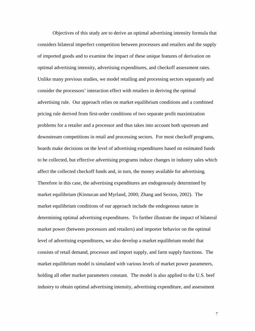
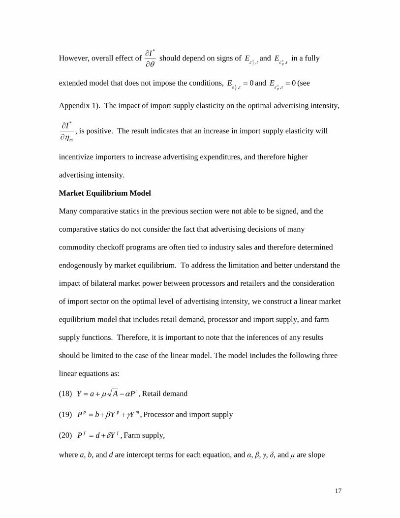
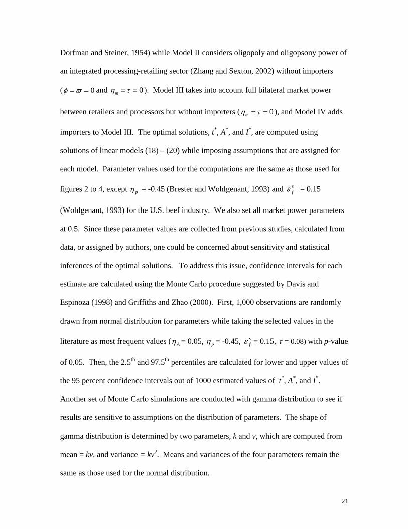
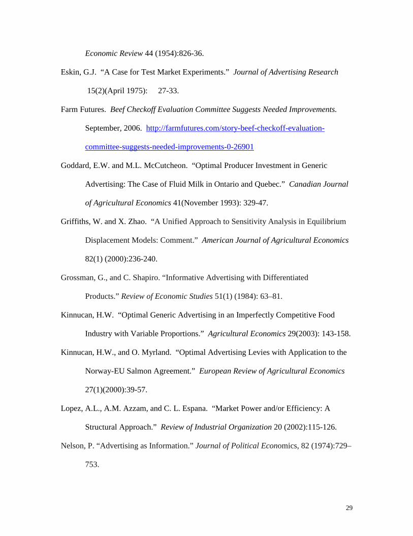
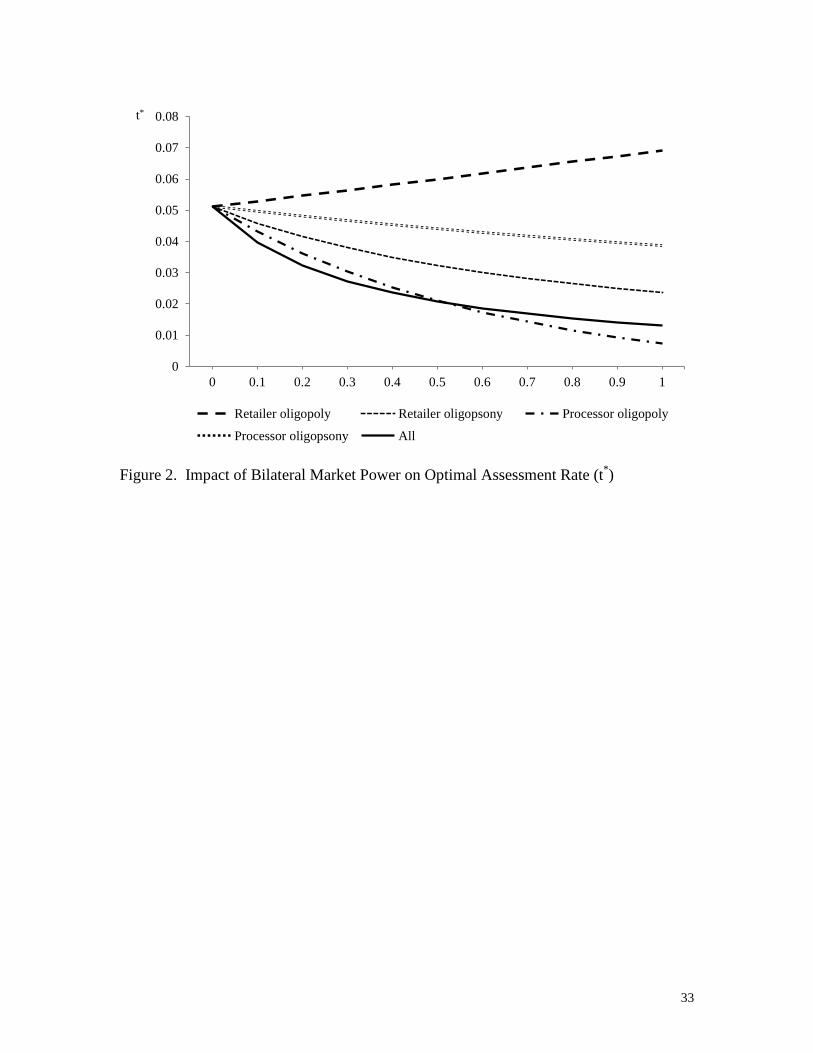
depicted in figures 2- 4. Figure 2 shows the impact of bilateral market power on optimal

assessment rate, t*. Zhang and Sexton (2002) report t* increases as a function of

oligopoly power exercised by an integrated retailing-processing sector. However, Figure

2 shows t* increases only with retailer’s oligopoly power while t*decreases with all other

market power parameters. Overall, t*decreases as the joint bilateral market power

between retailers and processors increases.

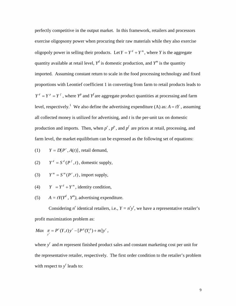
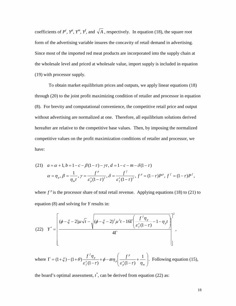
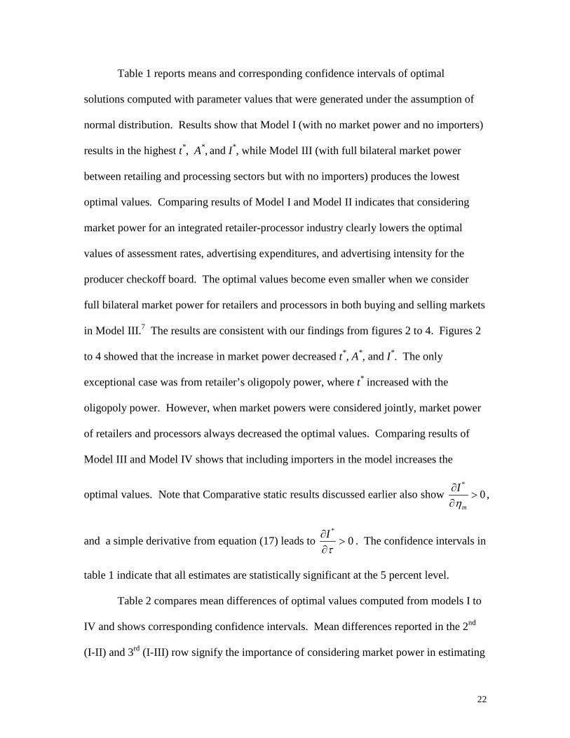
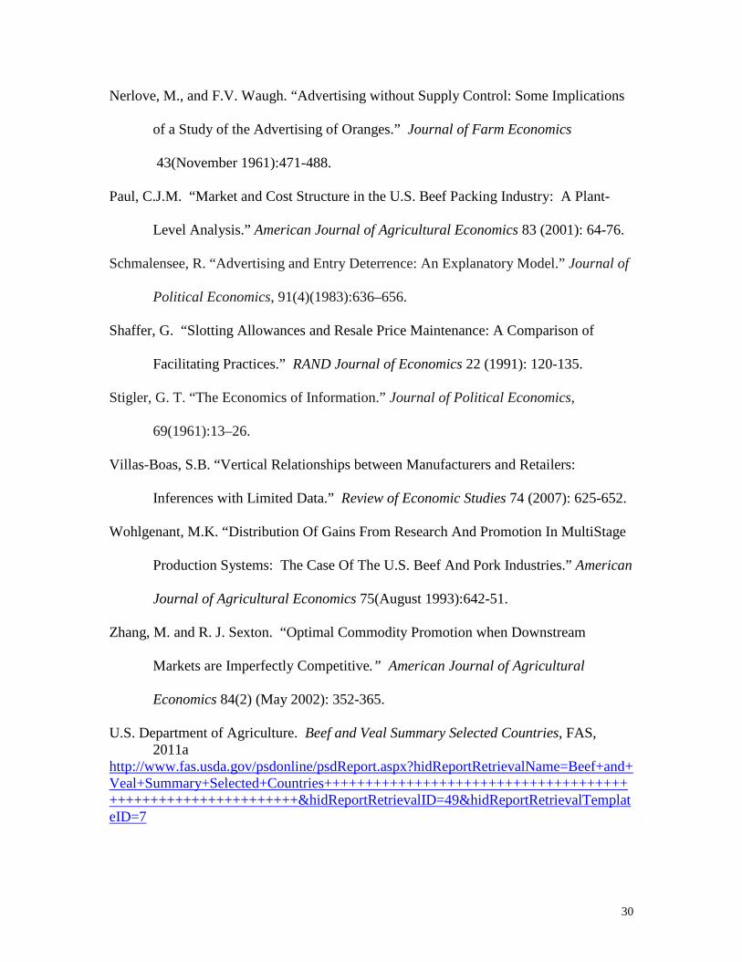
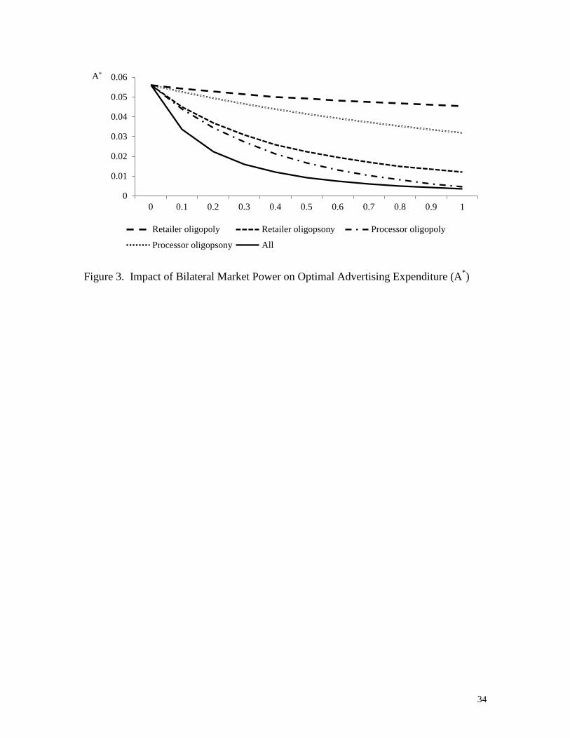
Figure 3 illustrates the impact of bilateral market power on the amount of optimal

advertising, A* = t*Y*. A*decreases with all market power parameters. The optimal

20

advertising expenditure decreases even with retailer oligopoly power because the

decrease in Y* (due to the increased market power) outweighs the increase in t* (see

Figure 2). It is straightforward that A* decreases with all other market power parameters

because both t*and Y* decreases as these market power parameters increase.

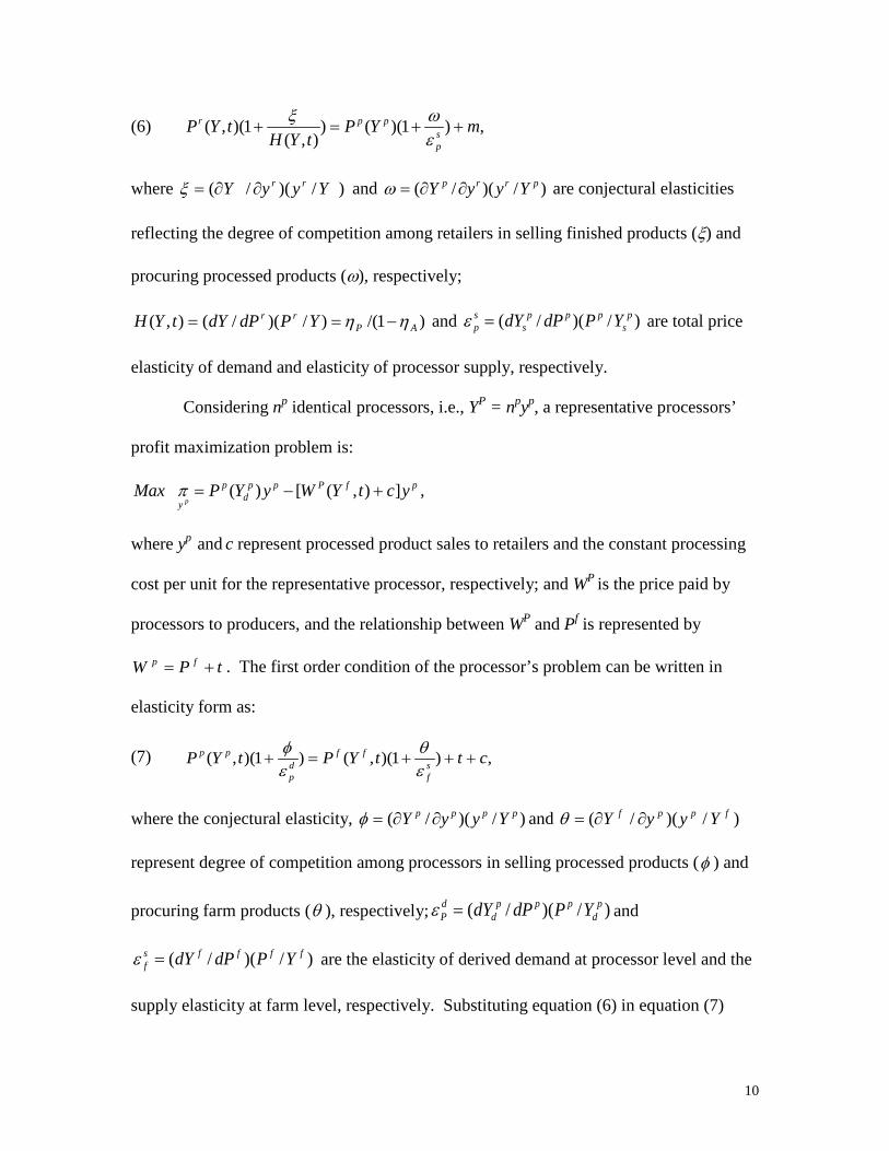
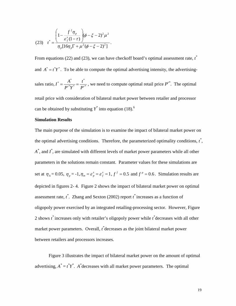
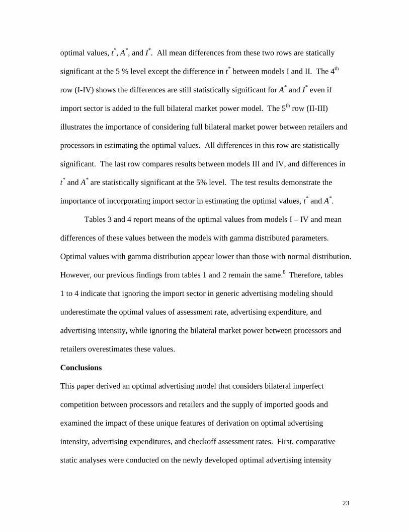
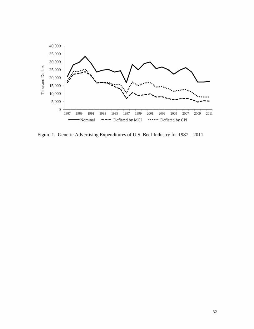
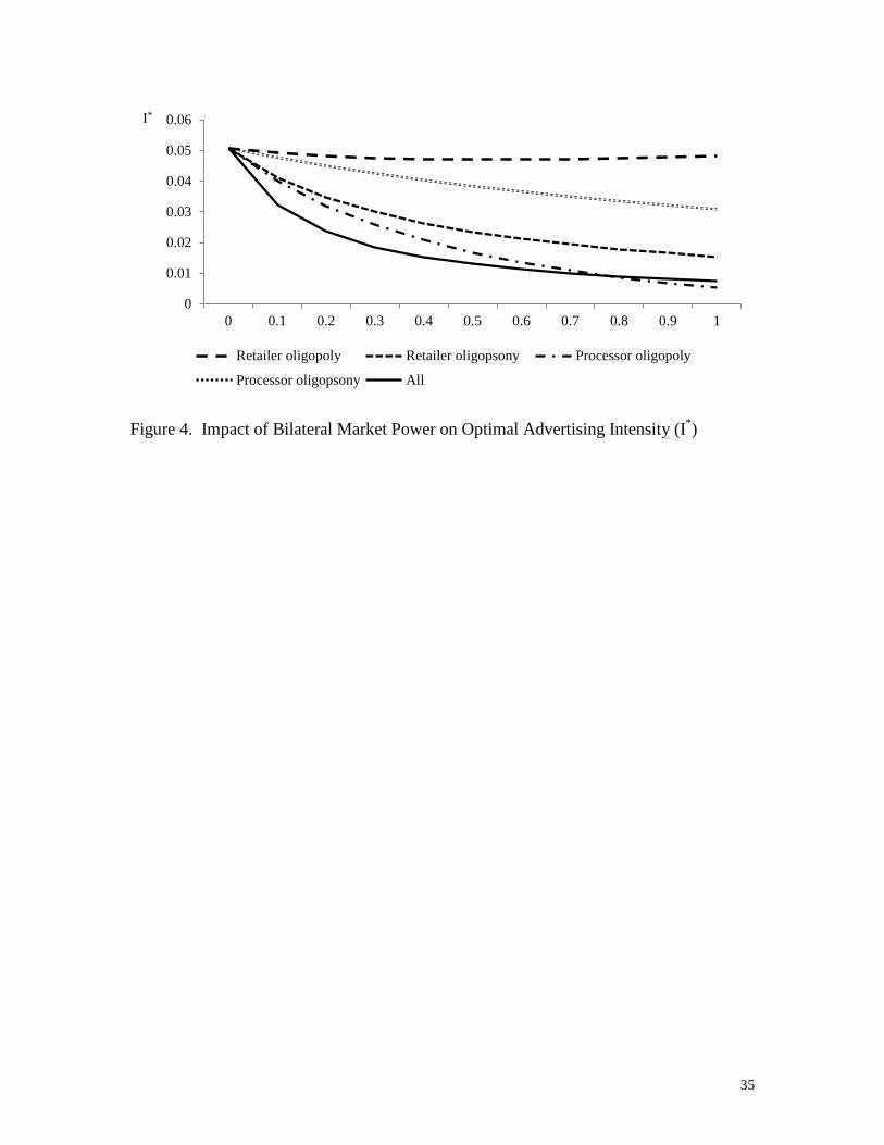
The impact of bilateral market power on the optimal advertising intensity,

*

*

**

**

rr Pt

YPAI == , is shown in Figure 4. I* slightly decreases as retailer’s oligopoly

power increases because the increase in Pr* (due to the increased market power) offsets

the increase in t*. For all other market power parameters, the increase in market power

decreases t* and increases Pr*, which results in the decrease in I*. In turn, when retailers

and processors increase their market power in either the buying or selling side, or both,

their profit-maximizing advertising intensity should decrease. Therefore, given that the

optimal advertising decision is made via a linear market equilibrium model constructed in

this section, overall the bilateral market power of retailing and processing sectors induces

the decrease in the optimal assessment rate, advertising spending, and advertising

intensity for the checkoff board. One exception is that the optimal assessment rate

increases with the oligopoly power of the retailing sector.

Another purpose of the simulation is to investigate whether the newly developed

procedure in this study produces different optimality conditions compared to alternative

procedures when retailers’ and processors’ bilateral market powers and the role of

importers are fully accounted. Four different models (including the one developed in this

study) are considered, and optimal solutions (assessment rate, advertising expenditure,

and advertising intensity) of each model are compared. Model I is a simple framework

without considering market power and importers (similar to the assumption used for

21

Dorfman and Steiner, 1954) while Model II considers oligopoly and oligopsony power of

an integrated processing-retailing sector (Zhang and Sexton, 2002) without importers

( 0==ϖφ and 0==τηm ). Model III takes into account full bilateral market power

between retailers and processors but without importers ( 0==τηm ), and Model IV adds

importers to Model III. The optimal solutions, t*, A*, and I*, are computed using

solutions of linear models (18) – (20) while imposing assumptions that are assigned for

each model. Parameter values used for the computations are the same as those used for

figures 2 to 4, except pη = -0.45 (Brester and Wohlgenant, 1993) and sfε = 0.15

(Wohlgenant, 1993) for the U.S. beef industry. We also set all market power parameters

at 0.5. Since these parameter values are collected from previous studies, calculated from

data, or assigned by authors, one could be concerned about sensitivity and statistical

inferences of the optimal solutions. To address this issue, confidence intervals for each

estimate are calculated using the Monte Carlo procedure suggested by Davis and

Espinoza (1998) and Griffiths and Zhao (2000). First, 1,000 observations are randomly

drawn from normal distribution for parameters while taking the selected values in the

literature as most frequent values ( Aη = 0.05, pη = -0.45, sfε = 0.15, τ = 0.08) with p-value

of 0.05. Then, the 2.5th and 97.5th percentiles are calculated for lower and upper values of

the 95 percent confidence intervals out of 1000 estimated values of t*, A*, and I*.

Another set of Monte Carlo simulations are conducted with gamma distribution to see if

results are sensitive to assumptions on the distribution of parameters. The shape of

gamma distribution is determined by two parameters, k and v, which are computed from

mean = kv, and variance = kv2. Means and variances of the four parameters remain the

same as those used for the normal distribution.

22

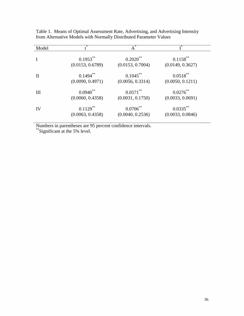
Table 1 reports means and corresponding confidence intervals of optimal

solutions computed with parameter values that were generated under the assumption of

normal distribution. Results show that Model I (with no market power and no importers)

results in the highest t*, A*, and I*, while Model III (with full bilateral market power

between retailing and processing sectors but with no importers) produces the lowest

optimal values. Comparing results of Model I and Model II indicates that considering

market power for an integrated retailer-processor industry clearly lowers the optimal

values of assessment rates, advertising expenditures, and advertising intensity for the

producer checkoff board. The optimal values become even smaller when we consider

full bilateral market power for retailers and processors in both buying and selling markets

in Model III.7 The results are consistent with our findings from figures 2 to 4. Figures 2

to 4 showed that the increase in market power decreased t*, A*, and I*. The only

exceptional case was from retailer’s oligopoly power, where t* increased with the

oligopoly power. However, when market powers were considered jointly, market power

of retailers and processors always decreased the optimal values. Comparing results of

Model III and Model IV shows that including importers in the model increases the

optimal values. Note that Comparative static results discussed earlier also show 0*

>∂∂

m

Iη

,

and a simple derivative from equation (17) leads to 0*

>∂∂τI . The confidence intervals in

table 1 indicate that all estimates are statistically significant at the 5 percent level.

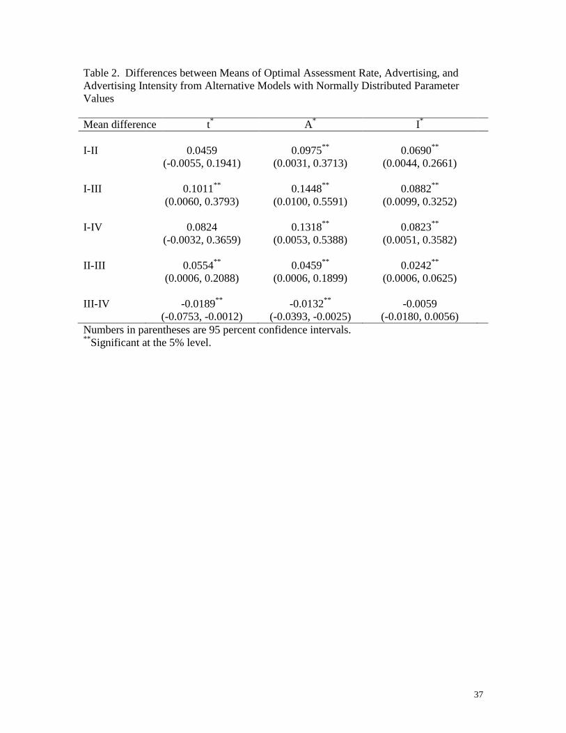
Table 2 compares mean differences of optimal values computed from models I to

IV and shows corresponding confidence intervals. Mean differences reported in the 2nd

(I-II) and 3rd (I-III) row signify the importance of considering market power in estimating

23

optimal values, t*, A*, and I*. All mean differences from these two rows are statically

significant at the 5 % level except the difference in t* between models I and II. The 4th

row (I-IV) shows the differences are still statistically significant for A* and I* even if

import sector is added to the full bilateral market power model. The 5th row (II-III)

illustrates the importance of considering full bilateral market power between retailers and

processors in estimating the optimal values. All differences in this row are statistically

significant. The last row compares results between models III and IV, and differences in

t* and A* are statistically significant at the 5% level. The test results demonstrate the

importance of incorporating import sector in estimating the optimal values, t* and A*.

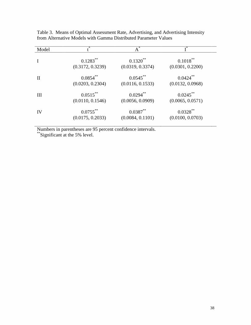
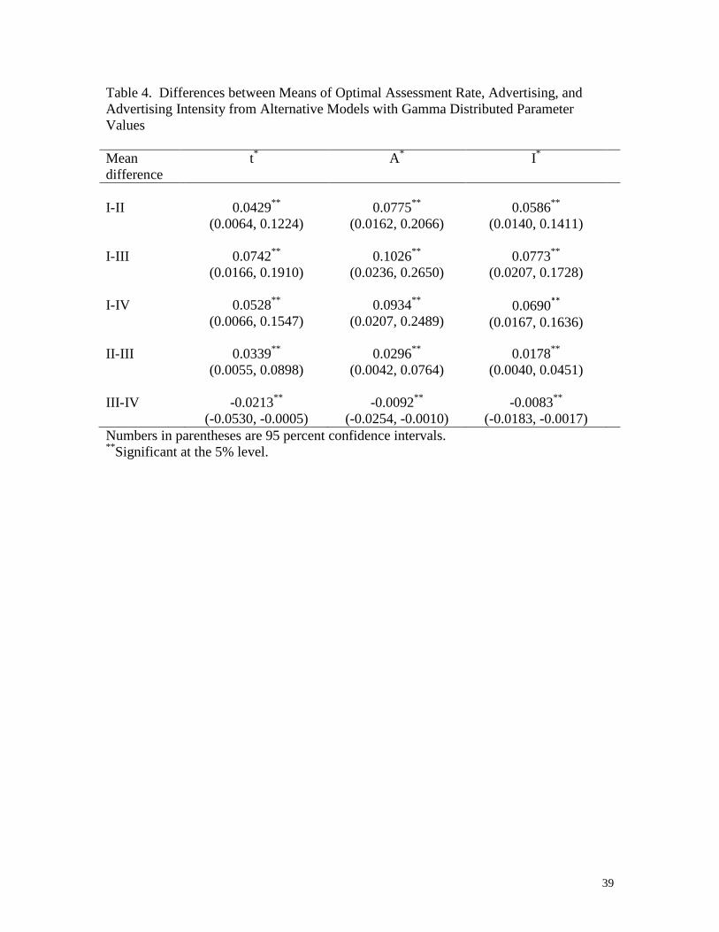
Tables 3 and 4 report means of the optimal values from models I – IV and mean

differences of these values between the models with gamma distributed parameters.

Optimal values with gamma distribution appear lower than those with normal distribution.

However, our previous findings from tables 1 and 2 remain the same.8 Therefore, tables

1 to 4 indicate that ignoring the import sector in generic advertising modeling should

underestimate the optimal values of assessment rate, advertising expenditure, and

advertising intensity, while ignoring the bilateral market power between processors and

retailers overestimates these values.

Conclusions

This paper derived an optimal advertising model that considers bilateral imperfect

competition between processors and retailers and the supply of imported goods and

examined the impact of these unique features of derivation on optimal advertising

intensity, advertising expenditures, and checkoff assessment rates. First, comparative

static analyses were conducted on the newly developed optimal advertising intensity

24

formula to examine the impact of bilateral market power and import supply on the

optimal advertising intensity. Second, a linear market equilibrium model that consists of

retail demand, processor and import supply, and farm supply equations were developed to

examine the impact of bilateral market power on the optimal advertising conditions.

Solutions from the linear market equilibrium model were simulated with different levels

of market power parameters while all other parameters in the solutions remain constant.

Finally, the linear equilibrium model was applied to the U.S. beef industry to obtain

optimal conditions of generic advertising, and results were compared to previous

approaches that did not consider bilateral imperfect competition and import sector.

Monte Carlo simulations were conducted to construct confidence intervals for sensitivity

analyses and statistical inferences of the results.

Impacts of changing bilateral market power parameters on advertising intensity

could not be signed from comparative static analyses in general. One exception was that

processor oligopsony power affected the optimal intensity positively when no supply

elasticity change caused by advertising was assumed at both processor and farm levels.

This finding is simply due to the contribution of the import sector to the intensity in

response to the processor’s oligopsony distortion. However, the overall impact of

changing the processor oligopsony power on the optimal advertising intensity could be

examined in a fully extended model without imposing any conditions on supply elasticity

change at both processor and farm levels. The impact of import supply elasticity on the

optimal advertising intensity was positive, which indicates that an increase in import

supply elasticity leads to importer’s higher incentive to advertising, and therefore, higher

advertising intensity. Simulation results of a linear market equilibrium model showed

25

that overall the bilateral market power of retailing and processing sectors induced the

decrease in optimal assessment rates, advertising spending, and advertising intensity for

the checkoff board. One exception was that the optimal assessment rate increased with

the oligopoly power of the retailing sector. Additional simulations were conducted to

compare the newly developed procedure with previous approaches that did not consider

bilateral imperfect competition and import sector. Comparing simulated estimates from

alternative procedures showed that the full consideration of retailer and processor

bilateral market power lowered the optimal advertising conditions while incorporating

importers in the model increased the optimal values. The simulated optimal values from

the new procedure were statistically different from those of previous procedures, in

general, and appeared not too sensitive to the assumption of probability distribution on

parameter values used in simulations. The simulation results signify the importance of

considering the retailer/processor bilateral market power and import supply in

determining optimal advertising conditions for commodity checkoff boards. Therefore,

based on comparative static results and simulation results from a linear market

equilibrium model, we conclude that optimal advertising conditions can be overestimated

without fully considering the bilateral market power while they can be underestimated

without import supply.

26

Footnotes 1. Clearly it is difficult to find an industry that satisfies these assumptions. However, as

Sexton (2000) correctly states, these simplifying assumptions do not bias the analysis of

competition in any particular direction and are made at no additional cost for generality.

2. Note that for brevity, we assume advertising has no impact on changing the elasticity

of processor demand and elasticities of processor and producer supply (i.e., ,0, =tdp

Eε

,0, =tsp

Eε

and

,0, =tsf

Eε

) which is similar to previous studies (Alston, Carman, and Chalfant,

1994; Zhang and Sexton, 2002; Kinnucan, 2003). The derivation for the case where

,0, ≠tdp

Eε

0, ≠tsp

Eε

, and 0, ≠tSP

Eε

is reported in Appendix 1.

3. More specifically, equation (17) is reduced to the Zhang and Sexton’s advertising-

sales ratio when 0==ϖφ (or ∞== sp

dp εε ) and 0==τηm .

4. From equation (7), 01 >

+ d

pεφ .

5. In the advertising literature, how advertising affects demand elasticity is unclear. One

school of thought is that advertising provides information about the existence of a brand

or about its quality, increases consumer awareness of attributes of brands and reduced

search costs, and thereby results in more elastic demand (Stigler, 1961; Nelsen, 1974;

Eskin, 1975; Grossman and Shapiro, 1984). The other school argues that advertising

creates product differentiations among brands that are otherwise difficult to distinguish.

The product differentiation creates a barrier to entry into a market, increases brand

loyalty, and reduces demand elasticity (Bain, 1956; Comanor and Wilson 1979;

Schmalensee, 1983).

27

6. The solution for Pr* is too long to present here. The solution can be provided upon

request.

7. One could argue that since Model II represents an integrated processing-retailing

sector, some portion of the market power parameters used in this model (ξ and θ ) may

be distributed to other bilateral market power parameters (φ and ϖ ) considered in Model

III and IV. To address this concern, we set the values of all market power parameters in

Model III and IV at 0.25 while maintaining ξ and θ in Model II at 0.5. Results show that

as expected, the optimal values from Model III and IV decrease (compared to those

reported in tables 1 and 2), but they are still significantly lower than those of Model II.

8. As we did in footnote 7, separate simulations were conducted with gamma distribution

to compute means and mean differences while setting the values of all market power

parameters in Model III and IV at 0.25 and ξ and θ in Model II at 0.5. As we observed in

footnote 7, overall findings remained the same under gamma distribution as well.

28

References

Alston, J.M., H.F. Carman, and J.A. Chalfant, “Evaluating Primary Product Promotion:

The Returns to Generic Advertising by a Producer Cooperative in a Small, Open

Economy,” Promotion in the Marketing Mix: What Works, Where, and Why.

Goddard and Taylor, Eds. University of Guelph: Toronto, 1994

Bain, J. Barriers to New Competition: Their Character and Consequences in

Manufacturing Industries. Cambridge: Harvard University Press, 1956.

Brester, G.W., and M.K. Wohlgenant. “Correcting for the Measurement Error in Food

Demand Estimation.” Review of Economics and Statistics 75(May 1993): 352-56.

Chung, C., and E. Tostao. “Nonparametric Estimation of Oligopsony Power in First-

Price Auction.” Journal of Agricultural Economics 60(2009): 318-333.

Chung, C., and E. Tostao. “Effects of Horizontal Consolidation under Bilateral Imperfect

Competition between Processors and Retailers.” Applied Economics 44(2012):

3379-3389.

Comanor, W.S., and T.A. Wilson. “The Effects of Advertising on Competition.” J.

Economic Literature 17 (1979): 453–476.

Davis, G.C., and M.C. Espinoza. “A Unified Approach to Sensitivity Analysis in

Equilibrium Displacement Models.” American Journal of Agricultural

Economics 80(4) (November 1998): 868-879.

Digal, L.N., and F.Z. Ahmadi-Esfahani. “Market Power Analysis in the Retail Food

Industry: A Survey of Methods.” The Australian Journal of Agricultural and

Resource Economics 46 (2002): 559-584.

Dorfman, R., and P.O. Steiner. “Optimal Advertising and Optimal Quality.” American

29

Economic Review 44 (1954):826-36.

Eskin, G.J. “A Case for Test Market Experiments.” Journal of Advertising Research

15(2)(April 1975): 27-33.

Farm Futures. Beef Checkoff Evaluation Committee Suggests Needed Improvements.

September, 2006. http://farmfutures.com/story-beef-checkoff-evaluation-

committee-suggests-needed-improvements-0-26901

Goddard, E.W. and M.L. McCutcheon. “Optimal Producer Investment in Generic

Advertising: The Case of Fluid Milk in Ontario and Quebec.” Canadian Journal

of Agricultural Economics 41(November 1993): 329-47.

Griffiths, W. and X. Zhao. “A Unified Approach to Sensitivity Analysis in Equilibrium

Displacement Models: Comment.” American Journal of Agricultural Economics

82(1) (2000):236-240.

Grossman, G., and C. Shapiro. “Informative Advertising with Differentiated

Products.” Review of Economic Studies 51(1) (1984): 63–81.

Kinnucan, H.W. “Optimal Generic Advertising in an Imperfectly Competitive Food

Industry with Variable Proportions.” Agricultural Economics 29(2003): 143-158.

Kinnucan, H.W., and O. Myrland. “Optimal Advertising Levies with Application to the

Norway-EU Salmon Agreement.” European Review of Agricultural Economics

27(1)(2000):39-57.

Lopez, A.L., A.M. Azzam, and C. L. Espana. “Market Power and/or Efficiency: A

Structural Approach.” Review of Industrial Organization 20 (2002):115-126.

Nelson, P. “Advertising as Information.” Journal of Political Economics, 82 (1974):729–

753.

30

Nerlove, M., and F.V. Waugh. “Advertising without Supply Control: Some Implications

of a Study of the Advertising of Oranges.” Journal of Farm Economics

43(November 1961):471-488.

Paul, C.J.M. “Market and Cost Structure in the U.S. Beef Packing Industry: A Plant-

Level Analysis.” American Journal of Agricultural Economics 83 (2001): 64-76.

Schmalensee, R. “Advertising and Entry Deterrence: An Explanatory Model.” Journal of

Political Economics, 91(4)(1983):636–656.

Shaffer, G. “Slotting Allowances and Resale Price Maintenance: A Comparison of

Facilitating Practices.” RAND Journal of Economics 22 (1991): 120-135.

Stigler, G. T. “The Economics of Information.” Journal of Political Economics,

69(1961):13–26.

Villas-Boas, S.B. “Vertical Relationships between Manufacturers and Retailers:

Inferences with Limited Data.” Review of Economic Studies 74 (2007): 625-652.

Wohlgenant, M.K. “Distribution Of Gains From Research And Promotion In MultiStage

Production Systems: The Case Of The U.S. Beef And Pork Industries.” American

Journal of Agricultural Economics 75(August 1993):642-51.

Zhang, M. and R. J. Sexton. “Optimal Commodity Promotion when Downstream

Markets are Imperfectly Competitive.” American Journal of Agricultural

Economics 84(2) (May 2002): 352-365.

U.S. Department of Agriculture. Beef and Veal Summary Selected Countries, FAS, 2011a http://www.fas.usda.gov/psdonline/psdReport.aspx?hidReportRetrievalName=Beef+and+Veal+Summary+Selected+Countries++++++++++++++++++++++++++++++++++++++++++++++++++++++++++++&hidReportRetrievalID=49&hidReportRetrievalTemplateID=7

31

U.S. Department of Agriculture. Livestock, Dairy, and Poultry Outlook, ERS, 2011b, http://www.ers.usda.gov/data-products/livestock-meat-domestic-data.aspx U.S. Department of Agriculture. Livestock, Dairy, and Poultry Outlook, ERS, 2011c, http://www.ers.usda.gov/data-products/dairy-data.aspx

32

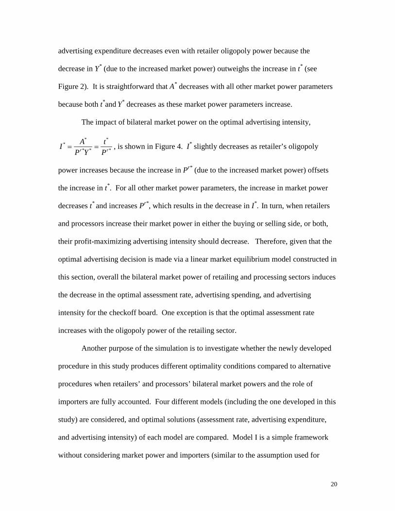
Figure 1. Generic Advertising Expenditures of U.S. Beef Industry for 1987 – 2011

0

5,000

10,000

15,000

20,000

25,000

30,000

35,000

40,000

1987 1989 1991 1993 1995 1997 1999 2001 2003 2005 2007 2009 2011

Thou

sand

Dol

lars

Nominal Deflated by MCI Deflated by CPI

33

Figure 2. Impact of Bilateral Market Power on Optimal Assessment Rate (t*)

0

0.01

0.02

0.03

0.04

0.05

0.06

0.07

0.08

0 0.1 0.2 0.3 0.4 0.5 0.6 0.7 0.8 0.9 1

Retailer oligopoly Retailer oligopsony Processor oligopoly

Processor oligopsony All

t*

34

Figure 3. Impact of Bilateral Market Power on Optimal Advertising Expenditure (A*)

0

0.01

0.02

0.03

0.04

0.05

0.06

0 0.1 0.2 0.3 0.4 0.5 0.6 0.7 0.8 0.9 1

Retailer oligopoly Retailer oligopsony Processor oligopoly

Processor oligopsony All

A*

35

Figure 4. Impact of Bilateral Market Power on Optimal Advertising Intensity (I*)

0

0.01

0.02

0.03

0.04

0.05

0.06

0 0.1 0.2 0.3 0.4 0.5 0.6 0.7 0.8 0.9 1

Retailer oligopoly Retailer oligopsony Processor oligopoly

Processor oligopsony All

I*

36

Table 1. Means of Optimal Assessment Rate, Advertising, and Advertising Intensity from Alternative Models with Normally Distributed Parameter Values Model t* A* I* I

0.1953**

(0.0153, 0.6789)

0.2020**

(0.0153, 0.7004)

0.1158**

(0.0149, 0.3627)

II 0.1494** (0.0090, 0.4971)

0.1045** (0.0056, 0.3314)

0.0518** (0.0050, 0.1211)

III 0.0940** (0.0060, 0.4358)

0.0571** (0.0031, 0.1750)

0.0276** (0.0033, 0.0691)

IV 0.1129** (0.0063, 0.4358)

0.0706** (0.0040, 0.2536)

0.0335** (0.0033, 0.0846)

Numbers in parentheses are 95 percent confidence intervals. **Significant at the 5% level.

37

Table 2. Differences between Means of Optimal Assessment Rate, Advertising, and Advertising Intensity from Alternative Models with Normally Distributed Parameter Values Mean difference t* A* I* I-II

0.0459

(-0.0055, 0.1941)

0.0975**

(0.0031, 0.3713)

0.0690**

(0.0044, 0.2661)

I-III 0.1011** (0.0060, 0.3793)

0.1448** (0.0100, 0.5591)

0.0882** (0.0099, 0.3252)

I-IV 0.0824 (-0.0032, 0.3659)

0.1318** (0.0053, 0.5388)

0.0823** (0.0051, 0.3582)

II-III 0.0554** (0.0006, 0.2088)

0.0459** (0.0006, 0.1899)

0.0242** (0.0006, 0.0625)

III-IV -0.0189** (-0.0753, -0.0012)

-0.0132** (-0.0393, -0.0025)

-0.0059 (-0.0180, 0.0056)

Numbers in parentheses are 95 percent confidence intervals. **Significant at the 5% level.

38

Table 3. Means of Optimal Assessment Rate, Advertising, and Advertising Intensity from Alternative Models with Gamma Distributed Parameter Values Model t* A* I* I

0.1283**

(0.3172, 0.3239)

0.1320**

(0.0319, 0.3374)

0.1018**

(0.0301, 0.2200)

II 0.0854** (0.0203, 0.2304)

0.0545** (0.0116, 0.1533)

0.0424** (0.0132, 0.0968)

III 0.0515** (0.0110, 0.1546)

0.0294** (0.0056, 0.0909)

0.0245** (0.0065, 0.0571)

IV 0.0755** (0.0175, 0.2033)

0.0387** (0.0084, 0.1101)

0.0328** (0.0100, 0.0703)

Numbers in parentheses are 95 percent confidence intervals. **Significant at the 5% level.

39

Table 4. Differences between Means of Optimal Assessment Rate, Advertising, and Advertising Intensity from Alternative Models with Gamma Distributed Parameter Values Mean difference

t* A* I*

I-II

0.0429**

(0.0064, 0.1224)

0.0775**

(0.0162, 0.2066)

0.0586**

(0.0140, 0.1411)

I-III 0.0742** (0.0166, 0.1910)

0.1026** (0.0236, 0.2650)

0.0773** (0.0207, 0.1728)

I-IV 0.0528** (0.0066, 0.1547)

0.0934** (0.0207, 0.2489)

0.0690** (0.0167, 0.1636)

II-III 0.0339** (0.0055, 0.0898)

0.0296** (0.0042, 0.0764)

0.0178** (0.0040, 0.0451)

III-IV -0.0213** (-0.0530, -0.0005)

-0.0092** (-0.0254, -0.0010)

-0.0083** (-0.0183, -0.0017)

Numbers in parentheses are 95 percent confidence intervals. **Significant at the 5% level.

40

Appendix 1. Advertising intensity with ,0, ≠td

pEε

0, ≠tsp

Eε

, and 0, ≠tSf

Eε

is derived as:

++

+−

+

−

+

+

−−

+

+

−

+

−+−

+

+

Φ=

dp

sp

dp

tH

p

dp

A

sf

sp

f

sfp

dp

mAsp

sf

f

dtp

stf

stp

cEH

E

HfE

Ef

YPA

εφϖ

εϖφ

εφξ

ηεφξη

τεεϖθ

τεηεφτηη

ϖφτ

εϖ

εθ

ε

ε

ε

111

11

)1(

1

)1(

1)(

)1(

11

1

,

,

,

2

,

2

**

*

where

+−

+

++

+−=Φ d

pdp

sp

sp

stp

dtp

EEεφϖ

εφ

εϖ

εϖφ

εε1111

,,