optimal feedback control formulation of the active noise...
TRANSCRIPT
Optimal Feedback Control Formulationof the Active Noise Cancellation Problem:
Pointwise and Distributed
Kambiz C. Zangi
RLE Technical Report No. 583
May 1994
Research Laboratory of ElectronicsMassachusetts Institute of TechnologyCambridge, Massachusetts 02139-4307
This work was supported in part by the U.S. Air Force Office of Scientific Research under GrantAFOSR-91-0034-C, in part by the U.S. Navy Office of Naval Research under GrantN00014-93-1-0686, and in part by a contract from Lockheed Sanders, Inc.

Optimal Feedback Control Formulation of the Active Noise Cancellation
Problem: Pointwise and Distributed
by
Kambiz C. Zangi
Submitted to the Department of Electrical Engineering and Computer Scienceon February 2, 1994, in partial fulfillment of the
requirements for degree ofDoctor of Philosophy
Abstract
Unwanted noise is a by-product of many industrial processes and systems. In
active noise cancellation (ANC), one introduces a secondary noise source to generate
an acoustic field that interferes destructively with the unwanted noise, and thereby
attenuates it. Noise reduction is important to protect listeners in high noise envi-
ronments from hearing damage, to enhance speech communication, and to reduce
noise-induced fatigue. These adverse effects of noise can cause accidents and reduce
the productivity of workers.
By formulating the ANC problem as an optimal feedback control problem, we
developed a single approach for designing stochastically optimal feedback controllers
for pointwise and distributed active noise cancellation. In the pointwise case, we
develop an optimal feedback controller for attenuating the acoustic pressure at the
locations of a finite number of microphones. In the distributed case, we develop an
optimal feedback controller for attenuating the total acoustic energy in an enclosure.
In either case, the control signal is pointwise and drives an ordinary loudspeaker, and
the input of the controller is pointwise and is obtained as the output of an ordinary
pressure microphone.
Thesis Supervisor: Alan V. OppenheimTitle: Distinguished Professor of Electrical Engineering
3


Dedicated to my parents.
5


Acknowledgment
I would like to express my most sincere thanks to Prof. Alan V. Oppenheim for his
mentoring, support, and guidance during the last four years. His superb management
of the Digital Signal Processing Group provided an ideal environment for me to work
on my thesis, and his insistence on creative and original work has influenced my
professional development greatly.
I am grateful to all the members of the Digital Signal Processing Group for their
friendship and moral support. I would like to particularly acknowledge Steven Is-
abelle, Paul Beckmann, Andy Singer, and Michael Richard. Interacting with them
has enriched my life both personally and professionally in numerous ways. I would
also like to thank Giovanni Aliberti and Stephen Scherock for their unfailing generos-
ity in devoting countless hours to solving my computer problems.
I am also indebted to my readers Prof. Sanjoy Mitter and Prof. George Verghese
for their involvement in the thesis. The assistance of Prof. Mitter with the distributed
control part of the thesis has been invaluable. Many thanks to Prof. Verghese for his
careful and timely review of the thesis. I am also grateful to Prof. Ehud Weinstein
of Tel Aviv University for sharing his technical insights on the topic with me.
My deepest thanks to Nathalie Tschudin for her emotional support, unending
patience, and sound advice. She filled my life with joy for the last ten years, and for
this I shall be grateful to her forever. Without her, this thesis would have not been
possible.
Finally, special thanks to my parents and my brother for their steadfast encour-
agement and support. Since I was born, my parents have willingly sacrificed so much
for my education. In recognition of their many sacrifices, this thesis is dedicated to
my parents.
7
i


Contents
1 Introduction 14
1.1 Outline of the Thesis . ............................. 16
2 Previous Work on Active Noise Cancellation 19
2.1 Introduction .................................... 19
2.2 Acoustical Principles ........................................... . 20
2.3 Control Strategies for ANC .......................... 26
2.3.1 Feedback Controllers for Active Noise Cancellation ......... . 26
2.3.2 Feedforward Controllers for Active Noise Cancellation ....... . 31
2.4 Performance Analysis for Two ANC Controllers ................ 36
2.4.1 Optimal Single-Channel Feedback Controller .................. . 37
2.4.2 Optimal Single-Channel Feedforward Controller ........... . 40
2.5 Relationship between Signal Estimation and Active Noise Cancellation . . . 42
2.5.1 Relationship between Single-Channel Signal Estimation and Single-
Channel ANC . . . . . . . . . . . . . . . . . . . . . . . . . . . . . . . 44
2.5.2 Relationship between Feedforward Signal Estimation and Feedfor-
ward ANC . . . . . . . . . . . . . . . . . . . . . . . . . . . . . . . . 48
2.6 Summary . . . . . . . . . . . . . . . . . . . . . . . . . . . . . . . . . . . . . 51
3 Pointwise Optimal Feedback Control for ANC 55
3.1 Introduction ......................................... 55
3.2 Single-Microphone Optimal Feedback Controller for ANC ......... ... . 57
3.2.1 Model Specification ........................... 58
9
---

3.2.2 The Optimal Feedback Controller. ...................
3.2.3 Frequency-Domain Perspective .....................
3.2.4 Frequency-Weighted Optimal Controller for ANC ...........
3.2.5 Implementation and Performance of the Optimal Feedback Controller
3.3 Multiple-Microphone Optimal Feedback Controller for ANC .........
3.4 Comparison of the Optimal Feedback Controller and the Optimal Feedfor-
ward Controller ..................................
3.5 Summary .....................................
4 Modeling of the Unwanted Noise at a Single Microphone
4.1 Introduction. .............................
4.2 Model Specifications .........................
4.3 Single-Microphone Recursive/Adaptive Identification Algorithm .
4.4 Algorithm Performance .......................
4.4.1 Synthetic Noise ........................
4.4.2 Aircraft Noise .........................
4.5 Summary ...............................
5 Distributed Optimal Feedback Control for ANC
5.1 Introduction .............................
5.2 Preliminaries .............................
5.2.1 General Properties of Semigroups ..............
5.2.2 Abstract Differential Equations: Cauchy Problem .....
5.3 Deterministic Linear Quadratic Regulator Problem ........
5.4 Dynamics of Two Deterministic Acoustic Systems .........
5.4.1 Purely Reflecting Boundaries ................
5.4.2 Purely Absorbing Boundaries ................
5.5 Abstract Representation of Two Deterministic Acoustic Systems
5.5.1 Purely Reflecting Boundaries ................
5.5.2 Purely Absorbing Boundaries ................
105
... . . . 105
... . .. 107
... . .. 107
... . . . 109
... . . . 113
... . . . 114
... . . . 116
... . . . 116
... . .. 117
... . . . 118
... . . . 120
10
62
66
67
69
72
81
87
89
...... .89
...... .90
...... .92
...... .97
...... .97
...... .98
...... 100

5.6 Stochastic Optimal Control for ANC ...................... 124
5.6.1 Preliminaries ............................... 124
5.6.2 Stochastic Quadratic Regulator Problem ................ 130
5.6.3 Abstract Representation of a Stochastic Acoustic System ..... . 133
5.7 Summary ............................................. 145
6 Conclusions and Future Directions 147
6.1 Summary and Contributions ....................................... 148
6.2 Future Directions . . . . . . . . . . . . . . . . . . . . . . . . . . . . . . . . 151
11
U


Chapter 1
Introduction
Unwanted noise is a by-product of many industrial processes and systems. In active noise
cancellation (ANC), one introduces a secondary noise source to generate an acoustic field
that interferes destructively with the unwanted noise, and thereby attenuates it.
Noise reduction is important to protect listeners in high noise environments from hearing
damage, to enhance speech communication, and to reduce noise-induced fatigue. These
adverse effects of noise can cause accidents and reduce the productivity of workers.
Passive silencers are low-pass acoustical filters commonly used on engines, blowers, com-
pressor, fans and other industrial equipment. These silencers are very effective in attenuat-
ing high frequency noise; however, they are usually bulky and ineffective at low frequencies.
This is because at low frequencies the acoustic wavelengths become large compared to the
thickness of a typical passive silencer. A sound wave of 60Hz, for example, has a wavelength
of 5.66 meters in air under normal conditions. It is also difficult to stop low frequency sound
being transmitted from one space to another unless the intervening barrier is very heavy.
Passive mufflers that are used to silence engine noise produce back-pressure by obstruct-
ing the turbulent flow out of the engine, and this back-pressure significantly reduces the
efficiency of the engine. To overcome these problems, researchers have given active noise
cancellation considerable attention recently.
The fundamental problem in ANC is to generate an acoustic field that interferes de-
structively with the unwanted noise field at the points of interest. A typical ANC system
13
--------------- - -----
utilizes several microphones to monitor the attenuated field and several canceling sources to
generate the canceling field. The outputs of these microphones are used as inputs to some
sort of electronic controller. This controller provides the inputs to the canceling sources in
such a way that the acoustic field generated by these sources interferes destructively with
the unwanted noise field at the points of interest.
Almost all existing ANC systems are designed explicitly to minimize the sum of the noise
power at a finite number of spatial points. We shall refer to this type of performance criterion
as a "pointwise performance criterion". Similarly, we refer to the resulting ANC system as
a "pointwise active noise cancellation system". In pointwise ANC, it is commonly assumed
that attenuating the noise at a finite number of spatial points will results in attenuation of
the noise at all other points of interest. However, it has been shown in numerical studies
that attenuation of noise at a finite number of spatial points can result in amplification of
the noise at other points [15].
Existing controllers for pointwise ANC can be characterized as feedforward or feedback
controllers. Adaptive feedforward controllers have been developed by a number of authors,
and these controllers are designed to take advantage of the statistics of the signals involved.
However, most existing feedback ANC systems are designed deterministically and do not
take advantage of the statistical characteristics of the noise.
A distributed active noise cancellation system is defined as an ANC system that mini-
mizes a distributed performance criterion. For example, a distributed ANC system might
minimize the total acoustic energy in an enclosure. To the best of our knowledge, a mathe-
matically rigorous procedure for designing distributed ANC systems has not been developed
yet.
By formulating the ANC problem as an optimal feedback control problem, we develop
a single approach for designing both pointwise and distributed ANC systems. The key
strategy is to model the residual signal/field as the sum of the outputs of two linear systems.
The unwanted noise signal/field is modeled as the output of a linear system driven by a
white process. Similarly, the canceling signal/field is modeled as the output of another
linear system driven by the control signal. Finally, the residual signal/field is modeled as
14

the sum of the outputs of these two linear systems. We show that the control signal that
minimizes a certain class of performance criteria is a linear feedback of the estimated states
of these two linear systems. These state estimates are computed using a Kalman filter, and
the feedback gain matrix/operator is obtained by iterating a Riccati equation. Note that
in the pointwise case and in the distributed case, the control signal is not distributed and is
used as input to an ordinary loudspeaker. Moreover in both these case, the control signal
is generated based on the outputs of ordinary microphones that monitor the residual field.
While we focus specifically on the acoustic noise cancellation problem, the results devel-
oped in this thesis can be applied to other active cancellation problems. Vibration control
is an example of a non-acoustic problem to which our results can be applied.
1.1 Outline of the Thesis
Chapter 2 motivates our study of active noise cancellation and presents a summary of
the previous work done in this area. The physics of the problem are discussed in this
chapter with emphasis on three dimensional acoustic fields. The different sound fields
generated by ANC systems designed to achieve different acoustic objectives are studied.
Several commonly used control strategies for ANC are presented, and the performance of
these control strategies are analyzed and compared. The relationship between active noise
cancellation and signal estimation is also discussed.
The optimal feedback controller for attenuating the acoustic pressure at a discrete num-
ber of microphone locations is developed in Chapter 3. Our approach is to model the
residual signals at the microphones as the sum of the outputs of two finite-dimensional
linear systems. The unwanted noise signals at the microphones are modeled as the outputs
of a multiple-input/multiple-output linear system driven by a white process. Similarly, the
canceling signals at the microphones are modeled as the outputs of a single-input/multiple-
output linear system driven by the control signal. Finally, the residual signals at the micro-
phones are modeled as the sum of the outputs of these two linear systems. We show that
the control signal that minimizes a certain class of performance criteria is a linear feedback
of the estimated states of these two linear systems. We also show that our formulation can
15
---------

be used to minimize the frequency weighted power of the residual signal. Such frequency
dependent weighting might be important because of the difference in the sensitivity of the
ear to sounds at different frequencies. These state estimates can be computed using a
Kalman filter, and the feedback gain matrix can be computed by iterating a matrix Riccati
equation. The single-microphone case is presented first, and the results are then extended
to the multiple-microphone case.
In Chapter 4, several recursive/adaptive algorithms for modeling the unwanted noise at
a single microphone are developed. We assume that the unwanted noise at the microphone
is the output of an all-pole transfer function driven by a white process and develop a
recursive/adaptive algorithm for estimating the parameters of this transfer function based
on the measurements made by the microphone. An adaptive feedback ANC system can be
obtained by combining the optimal control law of Chapter 3 with these recursive/adaptive
algorithms for modeling the unwanted noise. Although we focus specifically on developing
estimation algorithms for modeling the unwanted noise in the ANC problem, the algorithms
presented in this chapter can be applied to the more general problem of identifying non-
stationary autoregressive (AR) processes embedded in white noise.
Chapter 5 develops a distributed optimal feedback controller for minimizing the total
acoustic energy in an enclosure. Our approach is to model the residual field as the sum of the
outputs of two infinite-dimensional linear systems. The unwanted noise field is modeled as
the output of an infinite-dimensional linear system driven by a white process. Similarly, the
canceling field is modeled as the output of another infinite-dimensional linear system driven
by the control signal. Finally, the residual field is modeled as the sum of the outputs of these
two linear systems. The inputs to the controller are the outputs of ordinary microphones,
and the control signal drives an ordinary loudspeaker. We show that the control signal
that minimizes a certain class of performance criteria is a linear feedback of the estimated
states of these two linear systems. These state estimates can be computed using a Kalman
filter, and the feedback gain operator can be computed by iterating an operator Riccati
equation. This is the first mathematically rigorous formulation of the distributed ANC
problem known to us.
16

Lastly, in Chapter 6 we summarize the major contributions of this thesis. We also
suggest several potentially important directions for future research.
17
Chapter 2
Previous Work on Active Noise
Cancellation
2.1 Introduction
This chapter motivates our study of active noise cancellation and presents a summary of
the previous work done in this area. We try to distinguish between the acoustic objectives
of different ANC systems and the control strategies used to achieve these objectives. To
appreciate the advantages and the limitations of active noise cancellation, it is necessary
to understand the relevant acoustical principles as well as the relevant control strategies.
Hence, this chapter includes a Section on acoustical principles behind ANC and a Section
on control strategies used for ANC. The relationship between active noise cancellation and
signal estimation is also studied in this chapter.
This chapter is organized as follows. Section 2.2 describes the physical basis for active
noise cancellation, with emphasis on three dimensional sound fields. The different sound
fields that are generated by ANC systems designed to achieve different acoustic objectives
are studied in this Section using Modal Analysis techniques. In Section 2.3, we review several
commonly used control strategies for ANC. Many examples of existing ANC systems are
presented to illustrate the use of these control strategies. In Section 2.4, the performance
of two specific control strategies for ANC is analyzed in detail. Finally in Section 2.5, the
18

relationship between active noise cancellation and signal estimation is explored. A brief
summary of this chapter is presented in Section 2.6.
2.2 Acoustical Principles
The fundamental problem in active noise cancellation is to generate an acoustic field that
interferes destructively with the undesired noise [10, 13, 23, 40, 50, 59]. The undesired field
is usually referred to as the "primary" field, and the interfering field is referred to as the
"secondary" field. The question therefore arises as to whether two different sources of sound
can generate the same acoustic field? If the answer to this question is yes and one source is
under our control, a simple change of sign of the controlled source will cancel the primary
field everywhere.
We shall give a simple example of two different sources that generate the same acoustic
field. Let q(x, t) denote a sound source generating the pressure field p(x, t), where x is
the spatial variable; t is the temporal variable; and the underline denotes a vector-valued
quantity. Furthermore, assume that the source is only non-zero over some bounded spatial
domain r. In this case, the wave equation for pressure is
1 2 p(_,t) _ V 2 p(x,t) = q(x,t), (2.1)c2 &t2
where V2 is the three dimensional Laplacian, and c is speed of sound. The pressure field
p(x, t) outside the region of support of the source will remain unchanged if the source field
is supplemented by q(x,t)- V 2q(x, t). To see this, note that the resulting pressure
field in this case, p'(x, t), must satisfy
1 2 1 2 .
2 p'(X,t) - V 2 p'(x,t) = q(x, t) + -2 ~q(x,t) - V2 q(x,t), (2.2)
and eq. (2.2) can be rewritten as
1 2c20t2 (p'(x, t) - q(x , -t)) = q(x, t). (2.3)
Comparing (2.3) to (2.1) and recalling that q(x,t) is zero outside F, we conclude that
p'(x, t) and p(x, t) are equal outside F. Therefore, we have found an example of two distinct
sources that produce the same acoustic pressure field.
19
More generally, Kempton [31] has shown that the sound field generated by any source
can be reproduced by an appropriate infinite series of source singularities positioned at
any desired point. Hence, complete cancellation of the primary field can be achieved by
arranging these source singularities to produce the negative of the primary field.
A more obvious way to cancel the effect of an acoustic source is to use Kirchhoff's
theorem. This theorem provides a formula by which the entire effect of sources inside a
closed boundary can be duplicated by sources on this boundary. Hence, if the negative of
these sources is used on the boundary, the primary field in the exterior of the boundary
is completely canceled. Jessel and Angevine [28, 29] have proposed such an ANC system
in theory. Unfortunately, the secondary source in this case is distributed, and a discrete
approximation to this distributed source has not been developed yet. Inspired by this theory,
several researchers have built experimental ANC systems with limited success [4, 32].
With active noise cancellation, the combined radiated output of the primary and sec-
ondary sources is typically much less than the radiated output of the primary source alone.
The reduction in the combined radiated power is achieved by a reduction in the radiation
impedance seen by the primary source and/or absorption of energy by the secondary source
[17, 46].
Because of the practical difficulties associated with cancellation of an entire noise field,
most researchers have focused on developing ANC systems with very limited acoustic ob-
jectives. The most commonly used acoustic objective is attenuation of pressure at a finite
number of spatial points.
Modal analysis is one of the very few techniques avaiable for studying the global effects
of ANC in an enclosed volume.
Modal Analysis for ANC
Modal analysis is a practical approach for analyzing the sound field generated by an acoustic
system operating in an enclosure. The starting point is to assume that the sound field in the
enclosure has a periodic time dependence ej m . Let P(x, t) refer to the pressure at location
20

x and at time t. In this case, P(x, t) can be expressed as
P(x, t) = p(x, )ej t, (2.4)
where p(x, Q) is not a function of time. It is further assumed that p(x, Q) can be expressed
in terms of a finite number of the normal modes of the enclosure
N
p(x, Q) = Z .(x)a.(Q), (2.5)n=O
where n(x) is the the n-th normal mode of the enclosure, and an(Q) is the complex
amplitude of the n-th mode.
Next, it is assumed that the sound field is linear so that the complex amplitude a(Q)
can be expressed as the sum of the contributions from the primary source and M secondary
sources, i.e.M
an(Q) = aP(Q) + E Bnm()qs(Q), (2.6)m=1
where a(Q) is the n-th modal amplitude produced by the primary source; q((Q) is the net
strength of the m-th secondary source; and Bnm(fQ) specifies the degree to which the m-th
secondary source contributes to the n-th mode.
Equation (2.6) can be rewritten in vector form as
a = aP + Bqs, (2.7)
where a is the N x 1 vector
al(Q)
a2(Q)
aN(Q)
~~~~~; ~(2.8)
21
a =

aP is the N x 1 vector
qS is the M x 1 vector
and B is the N x M matrix of complex modal coupling coefficients
B11 (Q) ... B1m(Q)
B = ·' . (2.11)
BN1(Q) ... BNM(Q)
The total time-averaged acoustic potential energy in the enclosure is denoted by Ep and
is given by
Ep= jp(x, Q)Idx, (2.12)4c2p iv -
where c is the speed of sound, and p is the density of fluid in the enclosure. Recalling the
orthonormality of 4,'s, we see that
i 121 NEp= 2Ela(Q)I (2.13)
1 H (2.14)- 4c2paHa_.
Using the above formulation, one can find the secondary source strength q that min-
imizes the acoustic potential energy Ep. Since Ep is a quadratic function of the source
22
a p =
a(Q)
aPN( Aa()a()NA )
(2.9)
s =
q~(~)q1S (Q)
2q (Q)-qMS(9)
(2.10)

strength vector qS, the following source strength vector minimizes the total acoustic poten-
tial energy in the enclosure
qs = -[BHB]- B HaP, (2.15)
and the resulting minimum value of the potential energy is
Ep = 41 2 p[(a)aP - (aP)HB[BHB]-BHaP]. (2.16)
A similar formulation can be used to express the total acoustic kinetic energy in the
enclosure, Ek, as a quadratic function of the source strength vector qS. Furthermore, one
can find the secondary source strength that minimizes Ek or (Ek + Ep). Note that (Ek + Ep)
is the total acoustic energy in the enclosure.
Nelson et al. [36] considered the problem of minimizing the acoustic potential energy in
a rectangular enclosure. The three dimensional sound field in the enclosure was expressed
as the sum of the contributions of 7000 modes. Given the position and the strength of a
pure tone primary source (a point source), the authors used equation (2.15) to find the
amplitude and phase of a number of secondary point sources that would minimize the total
acoustic potential energy in the enclosure.
At frequencies above the Schroeder cut-off frequency of the enclosure, the authors found
that substantial reductions in acoustic potential energy are not obtainable unless the can-
celing sources are separated from the primary source by a distance of no more than half the
wave length [9].
At frequencies below the Schroeder cut-off frequency of the enclosure, the system exhib-
ited several interesting features [19]. The authors found that appreciable reductions in the
overall potential energy can be achieved by introduction of a small number of secondary
sources spaced greater than half a wavelength from the primary source, provided that the
enclosure is being excited at or near to acoustic resonance (where a single mode dominates
the response). In the low frequency case, the location of the canceling sources was found
to have a great influence on the performance of the system. It was found that at excitation
frequencies where only a single mode dominates the response of the enclosure, very large
reductions in potential energy can be achieved. On the other hand, at excitation frequencies
23
where many modes contribute to the response of the enclosure, a few secondary sources are
unable to control these modes without increasing the excitation of a number of other modes;
hence, little reduction in the total acoustic potential energy is achieved.
David [15] used a secondary point source to drive the acoustic pressure to zero at a
single point in a rectangular enclosure and studied the result of this action on the rest of
the sound field in the enclosure. He found that a "zone of quiet" around the cancellation
point, within which the sound pressure level is reduced by more than 15dB, has a diameter
of about one tenth of the wavelength of the excitation frequency. The mean-square pressure
away from the point of cancellation was found to increase if the transfer impedance between
the secondary source and the cancellation point was very small at the excitation frequency.
This led the authors to conclude that the secondary sources should be placed close to the
cancellation point to avoid increasing the mean-square pressure away from the cancellation
point.
Similar studies have been performed for the free field case [37]. In these studies, the
primary source and the secondary sources are assumed to be in a free field environment
with the primary source radiating at a single known frequency. The secondary source
strengths that minimize the power output of the combination of primary and secondary
sources is then found, and the minimum value of the power output is calculated. It is found
that significant reduction in the combined power output may only be achieved if secondary
sources are placed within a distance of half a wavelength of the primary source.
It is important to note that in all these experiments the secondary source strengths
were calculated based on the exact knowledge of the strength of the primary source for
all time. Therefore, these results can only be used as rough guidelines for predicting the
global behavior of practical ANC systems in which the source strength is unknown. In a
practical ANC system, the source strength must be estimated causally based on the available
measurements.
A typical ANC system utilizes several microphones to monitor the attenuated field
and/or the primary field. The outputs of these microphones are used as inputs to some
sort of electronic controller. The controller is designed to drive the secondary sources in
24
such a way that the desired acoustic objective is achieved. The desired acoustic objective
of almost all existing ANC systems is to attenuate the sound pressure at a finite number of
spatial points. In the next Section, we will concentrate on the algorithms that are used by
the controller to achieve this specific acoustic objective.
2.3 Control Strategies for ANC
A recent bibliography of references for ANC contains over 3450 entries [27]; therefore, it is
not possible to cover each reference individually. However, most of these references describe
particular applications of ANC rather than new concepts. In this Section we concentrate
on those control strategies that are most commonly used in active noise cancellation, and
selected references are only cited to illustrate the use of these control strategies.
Most existing active noise cancellation controllers can be categorized as pointwise feed-
back controllers or as pointwise feedforward controllers. The specific pointwise feedback
controller and pointwise feedforward controller that we focus on in this thesis are presented
next.
2.3.1 Feedback Controllers for Active Noise Cancellation
A generic feedback controller of the type we focus on in this thesis is depicted in Fig. 2.1,
where the input to the controller e(t) is the sum of the plant output c(t) and the stochastic
disturbance n(t). The goal is to choose the control signal r(t), based on observations of
{e(r): r < t}, so that the residual signal at the plant output e(t) follows a desired trajectory.
Note that n(t), e(t) or r(t) can be scalar valued or vector valued. The important assumption
here is that the control signal is generated based on the measurements of the residual signal
at the plant output, and not based on direct measurements of the disturbance. In this case,
all the inputs to the controller contain a part due to the plant output.
An illustrative example of a feedback ANC system is the noise canceling headphone
developed by Wheeler [51]. Wheeler used an analog feedback system to reduce the sound
pressure fluctuations in a headphone close to the ear of the listener. The noise cancellation
environment and the corresponding block diagram are depicted in Fig. 2.2 and Fig. 2.3,
25

n(t)
'(t)
Figure 2.1: Generic feedback controller.
respectively.
Throughout this chapter we rely on the following model of the microphone. The output
of the microphone is assumed to be the value of the acoustic pressure field at the location
of the microphone, i.e. the microphone is assumed to measure the acoustic pressure at the
location of the microphone without any distortion [6].
In Fig. 2.3, plant G(s) represents the overall transfer function from the canceling loud-
speaker input r(t) to the value of the canceling field at the location of the microphone
c(t) and incorporates the transfer functions of the loudspeaker and the propagation path
between the loudspeaker and the microphone. The microphone output e(t) is the sum of
the unwanted noise at the location of the microphone n(t) and the canceling signal at the
location of the microphone c(t). The goal of the controller is to minimize the sound pres-
sure fluctuations as measured by the microphone, i.e. the controller is designed to minimize
E{e2 (t)}. Comparing Fig. 2.3 with Fig. 2.1, we see that the noise canceling headphone
developed by Wheeler is a scalar analog feedback controller.
Note that this system attenuates the noise power at the microphone, and it is assumed
26

that attenuating the noise at the microphone will result in noise attenuation at the ear of
the listener. In noise canceling headphones with low frequency noise, this assumption is
quite reasonable because the ear of the listener is only about 3 centimeters away form the
microphone [15].
Figure 2.2: Noise canceling headphone proposed by Wheeler.
In the system of Fig. 2.3, the noise field at the microphone without the noise cancellation
system is n(t). With the noise cancellation system, the noise field at the microphone is e(t).
The power spectra of these two signals are related by the closed-loop transfer function T(s)
that is defined as
1T(s) = 1- H(s)G(s)
1 -H(s)G(s) (2.17)
where H(s) is the transfer function of the controller. Specifically,
Pee(jfQ) = IT(jQ) 2 P~(jF), (2.18)
where Pee(ej o) is the power spectrum of e(t), and P(jf) is the power spectrum of n(t)
with fl being the continuous-time frequency variable. Looking at eq. (2.18), we see that to
achieve attenuation over a certain frequency band, T(jQ)l must be made small over this
27

n(t)
0t)
.......................................
Figure 2.3: Block diagram of the noise canceling headphone proposed by Wheeler.
band. Typically, the analog controller is designed so that the closed-loop system achieves
moderate noise attenuation (15dB) over a relatively wide range of frequencies (50Hz-500Hz)
[12, 51]. Note that due to its analog nature, the controller in Fig. 2.2 cannot be changed
once it is built.
A Discrete-Time Feedback Controller
A discrete-time version of the system in Fig. 2.2 has been proposed by Graupe [26]. Since
the controller proposed by Graupe is a discrete-time controller we assume throughout this
Section that the noise to be canceled, the canceling signal, and all other intermediate signals
are appropriately sampled. Consequently in this Section, "t" represents the normalized
sampling time. Note that up to this point, we have been using "t" as the continuous-time
variable. Occasionally this notation can be ambiguous; however, we think that in most
cases the reader will be able to resolve this ambiguity based on the context. Whenever this
ambiguity cannot be resolved based on the context, we explicitly state whether "t" denotes
the continuous-time variable or the discrete-time variable.
The block diagram for the system of Graupe is depicted in Fig. 2.4, where G(z) is
the overall transfer function from the canceling loudspeaker input r(t) to the value of the
28
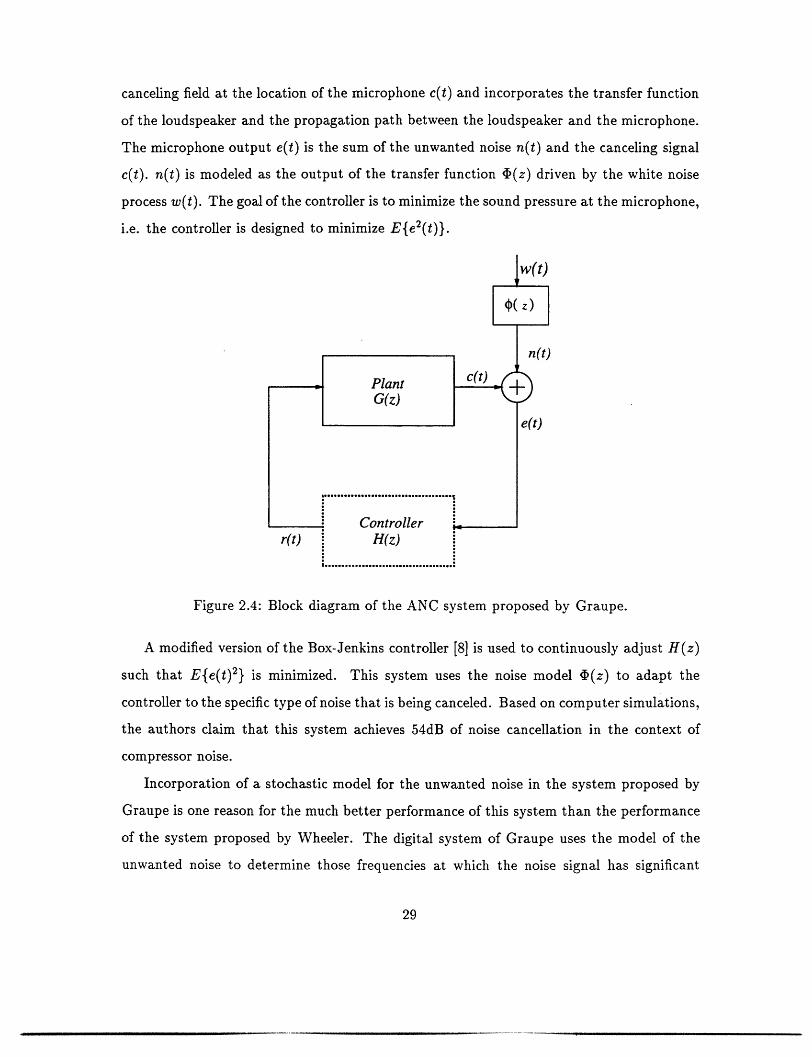
canceling field at the location of the microphone c(t) and incorporates the transfer function
of the loudspeaker and the propagation path between the loudspeaker and the microphone.
The microphone output e(t) is the sum of the unwanted noise n(t) and the canceling signal
c(t). n(t) is modeled as the output of the transfer function (z) driven by the white noise
process w(t). The goal of the controller is to minimize the sound pressure at the microphone,
i.e. the controller is designed to minimize E{e2 (t)}.
r(t) H(z)
Figure 2.4: Block diagram of the ANC system proposed by Graupe.
A modified version of the Box-Jenkins controller [8] is used to continuously adjust H(z)
such that E{e(t)2} is minimized. This system uses the noise model P(z) to adapt the
controller to the specific type of noise that is being canceled. Based on computer simulations,
the authors claim that this system achieves 54dB of noise cancellation in the context of
compressor noise.
Incorporation of a stochastic model for the unwanted noise in the system proposed by
Graupe is one reason for the much better performance of this system than the performance
of the system proposed by Wheeler. The digital system of Graupe uses the model of the
unwanted noise to determine those frequencies at which the noise signal has significant
29

energy, and it adjusts H(z) such that the resulting closed-loop transfer function, T(e jw) =
11-H(e.) G(e3w), is small over these frequencies. Since the compressor noise is extremely
narrow band, the resulting closed-loop system essentially acts as a notch filter. On the other
hand, the analog system proposed by Wheeler is fixed and makes no use of the spectral
characteristics of the unwanted noise; therefore, it achieves modest noise attenuation over
a wide range of frequencies.
The second reason for the excellent results obtained by Graupe is that his simulations
were performed with a G(z) that did not contain any delay. Moreover, the conroller proposed
by Graupe is derived based on the explicit assumption that G(z) contains no delay. This
severely limits the applications in which this algorithm can be used, since there are many
scenarios in which the propagation delay between the loudspeaker and the error microphone
is of the order of few sample intervals.
2.3.2 Feedforward Controllers for Active Noise Cancellation
A generic feedforward controller of the type we focus on in this thesis is depicted in Fig.
2.5, where q(t) is the input of the controller, and n(t) is the stochastic disturbance. The
goal is to choose the controller such that the residual signal at the plant output e(t) is as
close as possible to a desired trajectory. In this case, the input of the controller contains
no part due to the plant output c(t), i.e. there is no feedback from the plant output to the
inputs of the controller. This is in contrast to the feedback scheme of the previous Section
where the input of the controller was the sum of the plant output and the disturbance.
n(t)
q(t) " .......................I -f( )Feedforward I[ - - Controller I
;.. . ...............
Figure 2.5: Generic feedforward controller.
30
-------------------- -____ - _ ___ - -
Single-Channel Feedforward ANC Systems
Most of the early work in ANC was related to attenuation of duct noise at low frequencies
using feedforward controllers. A very thorough analysis of the duct problem was carried
out by Swinbanks in 1973 [49]. We shall present his work in some detail next because it
illustrates many of the issues involved in using feedforward controllers for ANC. The system
developed by Swinbanks is a continuous-time system; therefore, all the signals involved in
this Section are continuous-time signals.
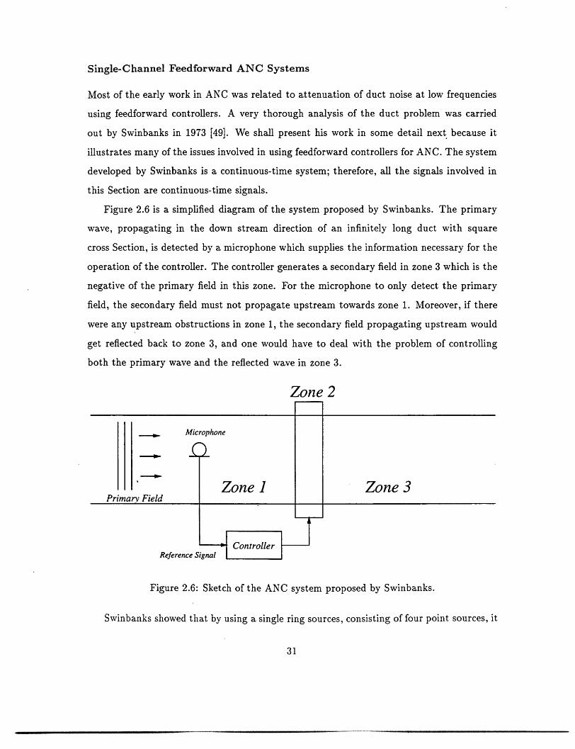
Figure 2.6 is a simplified diagram of the system proposed by Swinbanks. The primary
wave, propagating in the down stream direction of an infinitely long duct with square
cross Section, is detected by a microphone which supplies the information necessary for the
operation of the controller. The controller generates a secondary field in zone 3 which is the
negative of the primary field in this zone. For the microphone to only detect the primary
field, the secondary field must not propagate upstream towards zone 1. Moreover, if there
were any upstream obstructions in zone 1, the secondary field propagating upstream would
get reflected back to zone 3, and one would have to deal with the problem of controlling
both the primary wave and the reflected wave in zone 3.
Zone 2
| - | |Microphone
0 !
Primary FieldPrimary Field
Zone Zone 3
Reference Signal lU"LeI
Figure 2.6: Sketch of the ANC system proposed by Swinbanks.
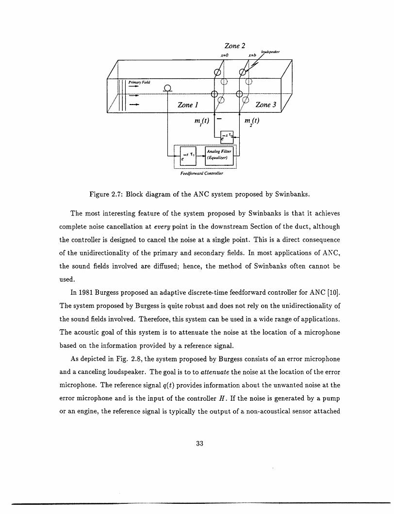
Swinbanks showed that by using a single ring sources, consisting of four point sources, it
31
i
I

is possible to generate an output consisting only of a propagating plane wave for frequencies
up to 2.1 times the cut-off frequency of the duct, see Fig. 2.7. More precisely, for these
frequencies, the non-plane wave modes in the duct will decay exponentially along the long
axis of the duct away from the ring source. Swinbanks also showed that by combining the
effects of two such ring sources, it is possible to generate an approximately unidirectional
plane wave in the duct up to 2.1 times the cut-off frequency of the duct, see Fig. 2.7.
Specifically, if the source strength of the upstream ring is ml(t) and the strength of the
downstream ring is m 2(t), there will be approximately zero output in the upstream direction
provided that
ml(t) = --m2(t-TO), (2.19)
where T0 is an appropriate amount of delay which depends on the separation between the
two rings and the speed of sound in the duct.
As illustrated in Fig. 2.7, the controller in this case consists of a delay element e"
followed by an analog filter whose purpose is to equalize the combined frequency response
of the secondary sources. Let p(x, t) denote the pressure field at location x (measured along
the long axis of the duct) and at time t. Over the frequency range of interest, the equalizer
tries to make p(b,t) = m 2(t- 2 ) for some delay 2 .
The operation of the ANC system of Swinbanks can be summarized as follows. At
time t, the controller predicts p(b,t + 72 ) and drives the equalized secondary sources with
the negative of this predicted value. If the prediction is perfect, the primary field and the
secondary field will interfere destructively at x = b, and the result will be complete silence
at this point. However, every other point in zone 3 will also be completely silent, since the
residual field in zone 3 is a plane wave propagating to the right.
Implementation of Swinbanks method, with minor modifications, resulted in a flurry of
publications (e.g., [7, 11, 41, 44]). These implementations showed that the main drawback
of Swinbanks' method is that very precise analog electronics are needed to implement the
feedforward controller. The required degree of precision in the magnitude and the phase of
the controller was found to be impossible to maintain except over a very limited range of
frequencies. In short, Swinbanks' method was found to lack robustness.
32
Zone 2
Feedforward Controller
Figure 2.7: Block diagram of the ANC system proposed by Swinbanks.
The most interesting feature of the system proposed by Swinbanks is that it achieves
complete noise cancellation at every point in the downstream Section of the duct, although
the controller is designed to cancel the noise at a single point. This is a direct consequence
of the unidirectionality of the primary and secondary fields. In most applications of ANC,
the sound fields involved are diffused; hence, the method of Swinbanks often cannot be
used.
In 1981 Burgess proposed an adaptive discrete-time feedforward controller for ANC [10].
The system proposed by Burgess is quite robust and does not rely on the unidirectionality of
the sound fields involved. Therefore, this system can be used in a wide range of applications.
The acoustic goal of this system is to attenuate the noise at the location of a microphone
based on the information provided by a reference signal.
As depicted in Fig. 2.8, the system proposed by Burgess consists of an error microphone
and a canceling loudspeaker. The goal is to to attenuate the noise at the location of the error
microphone. The reference signal q(t) provides information about the unwanted noise at the
error microphone and is the input of the controller H. If the noise is generated by a pump
or an engine, the reference signal is typically the output of a non-acoustical sensor attached
33

to the pump or the engine (e.g., a tachometer on the engine fly wheel). The controller is
a discrete-time finite impulse response system whose coefficients are continuously adjusted
to minimize the power of the residual signal e(t) at the error microphone.
e(t)
Prinmary Field
Error Microphon
Cancelling Loudspeaker
q(t) . fH ~
Reference Signal (FIR System) r(t)
Feedforward Controller
Figure 2.8: ANC system proposed by Burgess.
The block diagram for the system in Fig. 2.8 is depicted in Fig. 2.9, where q(t) is
the reference signal; H is the FIR controller whose coefficients at time "t" are {h(i,t)}L=;
and G(z) is the transfer function from the input of the loudspeaker r(t) to the value of
the canceling field at the location of the error microphone c(t). The output of the error
microphone e(t) is the sum of the unwanted noise at the location of the microphone n(t) and
the value of the canceling field at the location of the microphone c(t). This block diagram
is derived under the assumption that there is no feedback from the output of the canceling
loudspeaker to the reference signal.
j ............ :q(t) . H
. (FIR System) :
Feedforward Controller
Figure 2.9: Block diagram of the ANC system proposed by Burgess.
Assuming that G(z) is known, an LMS-type algorithm [52] can be derived for adjusting
the coefficients {h(i,t)}L=1 such that the mean-square power of the residual signal e(t) is
34

minimized. The update equations for the coefficients of the controller are:
h(i,t + 1) = h(i,t)- 2 l e(t) v(t - i) i = 1,...,L , (2.20)
where v(t) is defined as v(t) = fq(t) * g(t), and is the step-size of the algorithm. Note that
v(t) can be computed by "filtering" the known signal q(t) with the known impulse response
g(t); hence, this algorithm is sometimes referred to as the "filtered-x" algorithm [53].
Multiple-Channel Feedforward ANC Systems
A multiple-channel version of the algorithm of Burgess has been developed by Elliot et.
al [21, 18]. This algorithm is a discrete-time algorithm; therefore, all signals involved are
assumed to be appropriately sampled. As depicted in Fig. 2.10, this system consists of L
microphones and M loudspeakers. The controller in this case is a bank of M finite impulse
response filters {Hi}i 1 where each filter is driven by the reference signal q(t). The goal
is to adjust the coefficients of these filters such that a cost function involving the mean-
square sum of the microphone outputs and the mean-square sum of the control signals is
minimized. Specifically, given the matrix of transfer functions from the loudspeaker inputs
to the microphone outputs, the authors develop an LMS-type algorithm for adjusting the
coefficients of these M filters such that
L ME E (t) + a Er(t)
is minimized, where ca is a positive weighting coefficient for the control effort. Note that
the cost function used here is a bit more general than the one used by Burgess [10].
The influence of the loudspeaker transfer function and acoustic delay on the performance
of this algorithm has been thoroughly analyzed in a number of papers (e.g., [20, 47, 48]).
2.4 Performance Analysis for Two ANC Controllers
The performance of the continuous-time single-channel feedback ANC system and the per-
formance of the continuous-time single-channel feedforward ANC system are analyzed in
this Section.
35
------ --- - -

Feedforwrd Controller
Iq(r)
Figure 2.10: Multiple-channel feedforward ANC system.
2.4.1 Optimal Single-Channel Feedback Controller
Further insight about the continuous-time feedback ANC system of Wheeler [51] can be
gained by finding the optimal feedback controller in this case. Specifically in Fig. 2.3, we
would like to find the causal controller H(s) that minimizes E{e2 (t)}, assuming that the
noise n(t) is stationary with known power spectrum Pnn(jfl) and assuming that the plant
G(s) is known. Our strategy is to first find the minimizing controller within a restricted
class of controllers, and then show that no other controller can outperform this controller.
We shall make the further assumption that G(s) is stable. This is a reasonable assumption,
since the physical system that G(s) corresponds to is passive.
Let us start by looking at controllers of the form depicted in Fig. 2.11. In this figure,
G(s) (the transfer function of the plant) is fixed, and Q(s) is a causal and stable system that
can be varied subject to the restriction that the resulting closed-loop system must be stable.
Let us take an arbitrary controller within this class and assume that this controller results
36
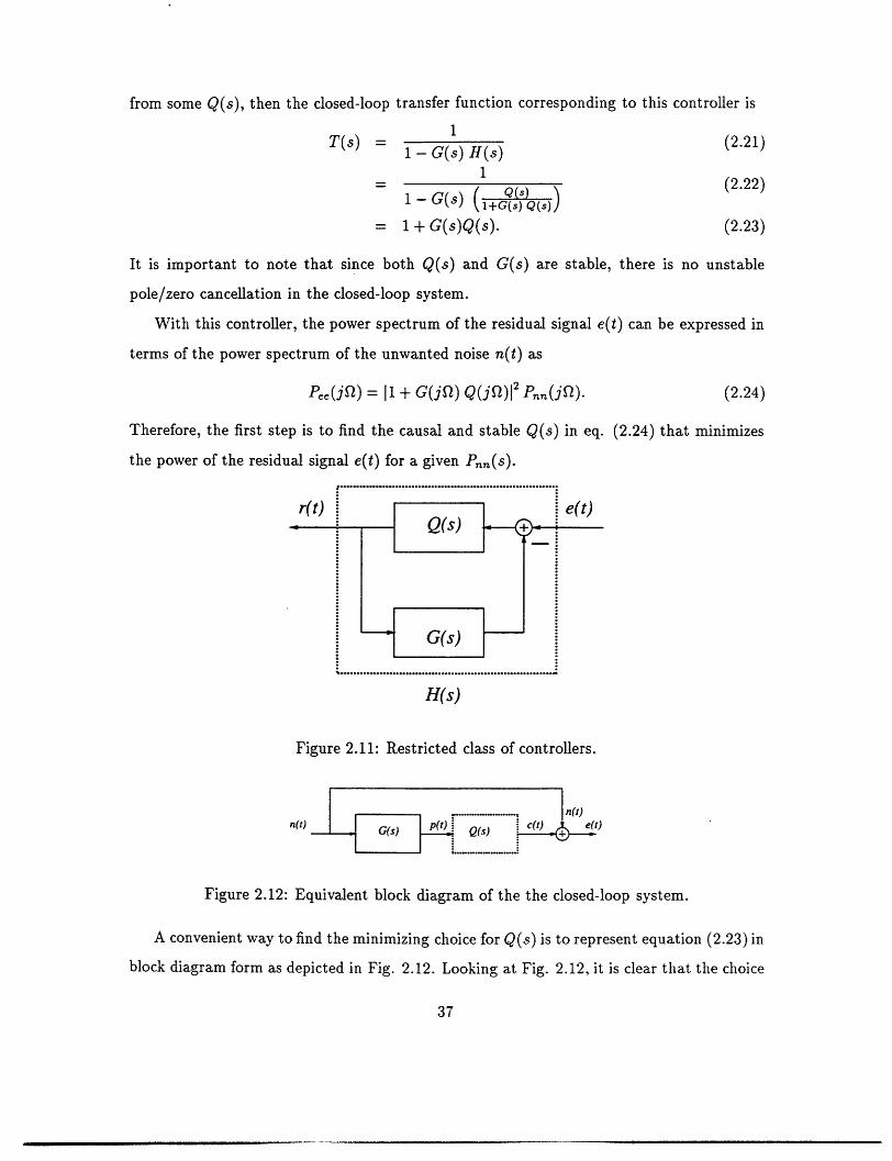
from some Q(s), then the closed-loop transfer function corresponding to this controller is
T() = 1 - G(s) H(s)_ ~11
1-G(s) (l+G(s) Q(. )
= 1 + G(s)Q(s).
(2.21)
(2.22)
(2.23)
It is important to note that since both Q(s) and G(s) are stable, there is no unstable
pole/zero cancellation in the closed-loop system.
With this controller, the power spectrum of the residual signal e(t) can be expressed in
terms of the power spectrum of the unwanted noise n(t) as
Pee(jf2) = I1 + G(jP) Q(ijQ) 2 P,,(jQ). (2.24)
Therefore, the first step is to find the causal and stable Q(s) in eq. (2.24) that minimizes
the power of the residual signal e(t) for a given Pnn(s).
H(s)
Figure 2.11: Restricted class of controllers.
r....................n()n(t) c(t) e(i)
G(s)IlP t )JQ(s)
Figure 2.12: Equivalent block diagram of the the closed-loop system.
A convenient way to find the minimizing choice for Q(s) is to represent equation (2.23) in
block diagram form as depicted in Fig. 2.12. Looking at Fig. 2.12, it is clear that the choice
37

for Q(s) that minimizes E{e 2(t)} is the causal Wiener filter [11] that produces the linear
least-squares estimate (LLSE) of-n(t) based on {p(r) < t}. Let us denote this particular
choice for Q(s) by Qwin(s), the corresponding controller by Hwi,.(s) = Ql+G(sQ-(s) and
the resulting E{e2 (t)} by Ei,. From eq. (2.23), we see that the closed-loop system in this
case is also stable, since G(s) and Qwi,i(s) are both stable.
It remains to be shown that no other causal controller can outperform Hij(s). We will
prove this by contradiction. To this end, assume that such a controller H#(s) exists, and
the resulting value of E{e2(t)} is E#, which is less than Ewin. It can be easily shown that
this leads to a contradiction by choosing
Q(S = 1- H#(s)(s) (2.25)
in Fig. 2.12 and noting that the resulting value for E{e2(t)} is E#, which is assumed to
be less than Ewi,. This is a contradiction, since E,- is obtained by minimizing E{e2(t)}
over all possible causal choices for Q(s). Note that Q(s) in eq. (2.25) is causal, since it can
be realized as feedback interconnection of H#(s) and G(s). Using the uniqueness of the
linear least-squares estimate, it can be shown that the canceling signal c(t) that minimizes
E{e2(t)} is unique.
This analysis shows that with the optimal controller, the canceling signal c(t) equals the
LLSE of-n(t) based on {p(r)'r < t}, where p(t) = n(t) * g(t). This analysis can be taken
one step further. To this end, let us express G(s) as
G(s) = Gaii(s)Gmin(s), (2.26)
where Gall(S) is an all-pass system function, and Gmin(s) is a minimum-phase system func-
tion. We also define p'(t) as
p'(t) = n(t) * gall(t). (2.27)
The LLSE of n(t) based on {p(r) r < t} is the same as the LLSE of n(t) based on
{p'(r) r < t}, since p(t) = p'(t) * gin(t) and Gmin(s) is minimum-phase. Recalling that
the minimizing choice for c(t) is the LLSE of -n(t) based on {p(r) : r < t}, we see that the
minimizing choice for c(t) can be alternatively expressed as the LLSE of -n(t) based on
38
{p'(r) : r < t}. Hence, the optimal performance of the noise cancellation system depends
on the joint second-order statistics of {n(t),p'(t)}, which can be calculate form the power
spectrum of n(t), since p'(t) = n(t) * gall(t) and gall(t) is known. Clearly, noise attenuation
will be high whenever p'(t) is highly correlated with n(t).
If the phase of Gall(s) is approximately linear over the frequencies for which n(t) has
significant energy, the problem will reduce to predicting -n(t) based on {n() r < t- to},
where ro is the slope of the linear approximation to the phase of Gall(s).
2.4.2 Optimal Single-Channel Feedforward Controller
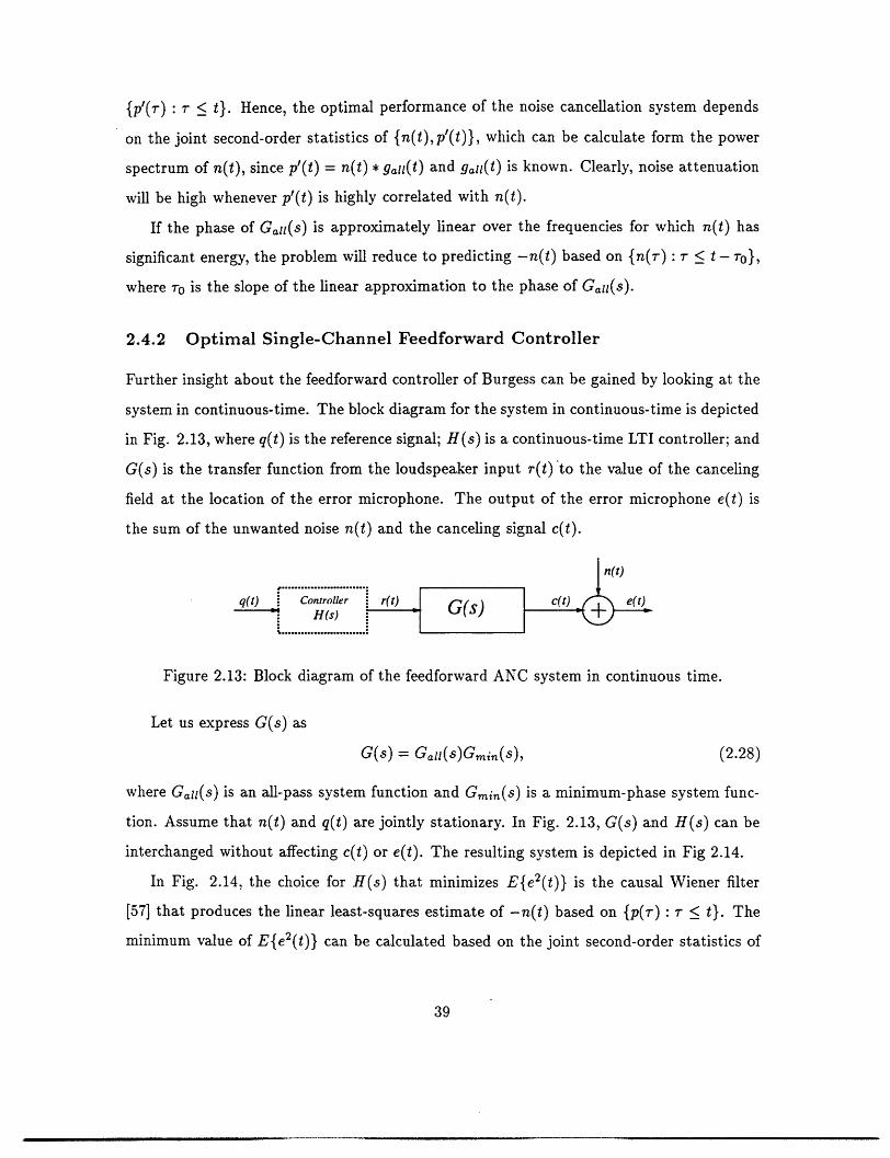
Further insight about the feedforward controller of Burgess can be gained by looking at the
system in continuous-time. The block diagram for the system in continuous-time is depicted
in Fig. 2.13, where q(t) is the reference signal; H(s) is a continuous-time LTI controller; and
G(s) is the transfer function from the loudspeaker input r(t)'to the value of the canceling
field at the location of the error microphone. The output of the error microphone e(t) is
the sum of the unwanted noise n(t) and the canceling signal c(t).
n(t): .................
q(t) Controller r(t) c( C. H(s) G(S)A...........................
Figure 2.13: Block diagram of the feedforward ANC system in continuous time.
Let us express G(s) as
G(s) = Gai(s)Gmin(S), (2.28)
where Gait(s) is an all-pass system function and Gmin(s) is a minimum-phase system func-
tion. Assume that n(t) and q(t) are jointly stationary. In Fig. 2.13, G(s) and H(s) can be
interchanged without affecting c(t) or e(t). The resulting system is depicted in Fig 2.14.
In Fig. 2.14, the choice for H(s) that minimizes E{e2(t)} is the causal Wiener filter
[57] that produces the linear least-squares estimate of -n(t) based on {p(r): r < t}. The
minimum value of E{e2(t)} can be calculated based on the joint second-order statistics of
39

{n(t), p(t)} , which in turn can be calculated based on the joint second-order statistics of
{n(t),q(t)}, since p(t) = q(t) * g(t) and g(t) is known.
G(s)
Figure 2.14: Alternate block diagram for the ANC system proposed by Burgess.
This analysis can be taken one step further by observing that the linear least-squares
estimate of n(t) based on {p(r): r < t} is equivalent to the linear least-squares estimate of
n(t) based on {p"(r) : r < t}, since p(t) = p"(t) * g,,in(s) and Gmin(s) is minimum phase.
Therefore, the noise attenuation will be high whenever p"(t) is highly correlated with n(t).
If the phase of Gal(s) is approximately linear over those frequencies for which q(t) has
significant energy, the problem will reduce to predicting -n(t) based on {q(r) : < t - ro}
where 0 is the slope of the linear approximation to the phase of Gaii(s). In this case, the
noise attenuation is substantial whenever q(t) is highly correlated with the future values of
n(t). Note that this approximation is quite reasonable whenever the noise to be canceled is
relatively narrow band.
A major shortcoming of the ANC system developed by Burgess is discussed next. The
above analysis implies that the system of Burgess works well whenever the reference signal
is highly correlated with the noise at the error microphone, and there is no feedback from
the canceling loudspeaker to the reference signal. However, the formulation of Burgess
does not tell us how to obtain such a reference signal. The author suggests the use of
non-acoustical sensors attached to the noise source. In many applications, the source of
the noise is inaccessible or unknown; hence, it is often not possible to acquire the reference
signal in this way.
A common practice advocated by many researchers is to use the output of a second
microphone (called the reference microphone) as the reference signal. Unfortunately, there
is typically some feedback from the canceling loudspeaker to the output of the reference
40

microphone. In the presence of this feedback, the algorithm proposed by Burgess no longer
minimizes E{e2(t)}; moreover, the overall system has been observed to go unstable in the
presence of this feedback. To decrease the feedback from the canceling loudspeaker to the
reference microphone, the reference microphone is usually placed far away form the canceling
loudspeaker and the error microphone. However, this decreases the correlation between the
noise at the error microphone and the noise at the reference microphone, resulting in low
levels of noise attenuation.
The multiple-channel feedforward ANC algorithm proposed by Elliot et. al [21, 18] suf-
fers from the same shortcoming that the single-channel algorithm of Burgess does. Specifi-
cally, there is the problem of how to acquire a reference signal that is highly correlated with
the unwanted noise and at the same time avoid acoustic feedback from the output of the
canceling loudspeakers to the reference signal.
To circumvent the acoustic feedback problem associated with the use of a reference
microphone, Eriksson et. al. [23] proposed an ANC system that takes the effect of the feed-
back into account in the design of the adaptive controller. Specifically, Eriksson proposed
canceling the effect of the feedback at the output of the reference microphone, i.e. the input
of the controller in this case is the sum of the output of the reference microphone and the
negative of the estimate of the feedback. The resulting system uses two LMS algorithms
and is quite complicated. More importantly, instability can result if the parameters of the
adaptive algorithm are arbitrarily set, and the authors offer no procedure for properly set-
ting these parameters. Furthermore, this system still works poorly whenever the noise at
the reference microphone is not highly correlated with the noise at the error microphone.
2.5 Relationship between Signal Estimation and Active Noise
Cancellation
The relationship between signal estimation and active noise cancellation is explored in this
Section.
Signal estimation refers to estimating one stochastic process from observations of another
41

stochastic process. The goal in signal estimation is to generate, based on an observed signal,
an output signal that is as close as possible to some desired signal. In a large class of
signal estimation problems, the desired signal and the output signal are both numerical
representation of some underlying physical signal. For example, in speech enhancement the
desired signal is a numerical representation of the pressure fluctuations produced by the
vocal cords of the speaker, and the output of the speech enhancement system is a numerical
estimate of these pressure fluctuations. In this class of problems, all the signals involved
(including the desired signal) are numerical; hence, there is no need to consider the physical
signals that these numerical signals represent. Moreover in this class of problems, the
process by which the output signal is obtained is purely numerical. In the reminder of this
Section the term "signal estimation" refers exclusively to this type of numerical estimation.
In active noise cancellation, the desired signal is a physical signal and not a numerical
signal; therefore, the output signal in active noise cancellation is also a physical signal.
Furthermore, the output signal in ANC is generated as the sum of a canceling signal and
one of the inputs. Since the output signal is a physical signal, the canceling signal and the
input signal to which the canceling signal is added are both physical signals as well. Hence,
every active noise cancellation system must have a transducer for physically generating the
canceling signal. If the input of this transducer is significantly different from its output, the
design of the ANC system must take the effect of the transducer into account.
For example, in acoustic active noise cancellation, the canceling signal and the unwanted
noise are both physical signals corresponding to the primary pressure field and the secondary
pressure field, respectively. The canceling signal is generated by a loudspeaker and is added
physically to the unwanted noise through the interference of the primary field and the
secondary field. Note that the process by which the output signal is obtained is not purely
numerical, since the output signal is obtained through physical interference of two acoustic
fields.
The relationship between signal estimation, in which the desired signal is a numerical
signal, and active noise cancellation, in which the desired signal is a physical signal, is
explored in this Section. In Section 2.5.1, a very general class of single-input/single-output
42
signal estimation systems is compared to the class of single-channel feedback ANC systems.
In Section 2.5.2, the class of single-channel feedforward ANC systems is compared to a
special class of two-input/single-output signal estimation systems.
2.5.1 Relationship between Single-Channel Signal Estimation and Single-
Channel ANC
The relationship between single-channel signal estimation and single-channel feedback active
noise cancellation is studied in this Section.
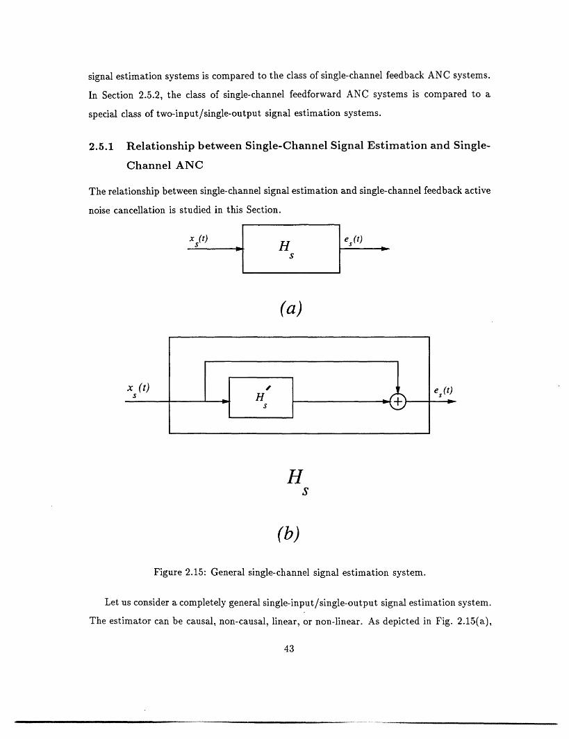
(a)
HS
(b)
Figure 2.15: General single-channel signal estimation system.
Let us consider a completely general single-input/single-output signal estimation system.
The estimator can be causal, non-causal, linear, or non-linear. As depicted in Fig. 2.15(a),
43

X(t)
ea (t
Feedback Controller
(a)
(b)
Figure 2.16: Feedback single-channel ANC system.
44
I
I( t)
this system is a single-input/single-output system with input x(t) and output e(t). The
objective is to find the system Hs that makes e(t) as close as possible to some desired
signal d(t). Alternatively, the single-channel signal estimation system can be expressed
in block diagram form as depicted in Fig. 2.15(b), where H = Hs - I with I being the
identity system. Referring to Fig. 2.15(b), the single-channel signal estimation problem can
be stated as follows:
Find the single-input/single-output system He that minimizes
J ({ [xs(r) + HI.(xS(T)), ds(r)] 0 < r < T}), (2.29)
where J(.) is a pre-specified cost function that indicates how close the output es(t) is to the
desired signal ds(t) over the time interval 0 < t < T, e.g.
J ({ [xS(') + H:(X(r)), da(T)] : < < T}) = (2.30)
f E { [x (T) + H'(X.(7)) - d8(7)] 2} d. (2.31)
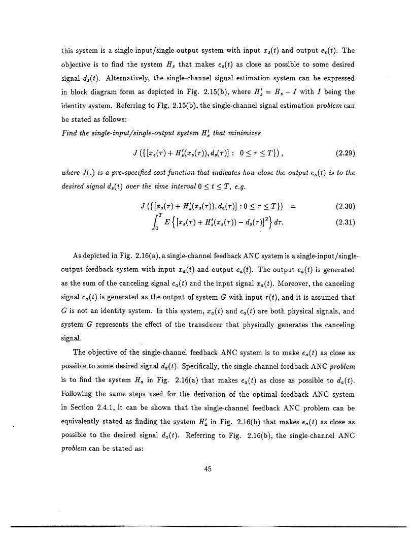
As depicted in Fig. 2.16(a), a single-channel feedback ANC system is a single-input/single-
output feedback system with input xa(t) and output ea(t). The output ea(t) is generated
as the sum of the canceling signal ca(t) and the input signal xa(t). Moreover, the canceling
signal c(t) is generated as the output of system G with input r(t), and it is assumed that
G is not an identity system. In this system, Xa(t) and c(t) are both physical signals, and
system G represents the effect of the transducer that physically generates the canceling
signal.
The objective of the single-channel feedback ANC system is to make e(t) as close as
possible to some desired signal da(t). Specifically, the single-channel feedback ANC problem
is to find the system Ha in Fig. 2.16(a) that makes ea(t) as close as possible to d(t).
Following the same steps used for the derivation of the optimal feedback ANC system
in Section 2.4.1, it can be shown that the single-channel feedback ANC problem can be
equivalently stated as finding the system H' in Fig. 2.16(b) that makes ea(t) as close as
possible to the desired signal da(t). Referring to Fig. 2.16(b), the single-channel ANC
problem can be stated as:
45

Find the single-input/single-output system H' that minimizes
J ({ [xa(r) + (GoH')(xa(r)), da(r)]: 0 < < T}), (2.32)
where "or is the composition operator.
Comparing the single-channel signal estimation problem to the single-channel feedback
ANC problem, we see that the ANC problem can be viewed as a constrained version of
the signal estimation problem. Specifically, the single-channel feedback ANC problem can
be formulated as finding H' that minimizes the expression in eq. (2.29) subject to the
constraint that Hi must be of the following form
H = GoH', (2.33)
for some system H' and a given system G.
We now compare the single-channel signal estimation system to the single-channel feed-
back ANC system in terms of their input/output characteristics. To this end, we assume
that both systems are driven by the same input and that the desired signal for both systems
is the same. We also assume that each system is designed so that the the distance between
its output and the desired signal is minimized.
Under these assumptions, the performance of the ANC system is never better than the
performance of the corresponding signal estimation system, since the optimal ANC system
is obtained by minimizing J(.) subject to a constraint, while the optimal signal estimation
system is obtained by minimizing J(.) without any constraints.
Again under these assumptions, if the minimizing H' in eq. (2.29) happens to equal
(GoQ) for some system Q, the optimal ANC system will be identical to the optimal signal
estimation system. Specifically, in this case, the minimizing H' in the ANC problem is
system Q. For example, if G is invertible, the minimizing H' can be expressed as
H = IoH' (2.34)
= Go(G-loH'), (2.35)
where I is the identity system. This implies that the solution to the single-channel feedback
ANC problem can be expressed in terms of the solution to the corresponding single-channel
signal estimation problem with H' = G-loH'.
46
The above discussion implies that unless the solution to the signal estimation problem
is (GoH') with H' begin the solution to the corresponding ANC problem, the optimal
feedback ANC system will be different from the optimal signal estimation system.
In general, a procedure for solving the single-channel signal estimation problem cannot
be used to solve the single-channel feedback ANC problem, since a procedure for solving an
un-constrained minimization problem cannot be used to solve a constrained minimization
problem.
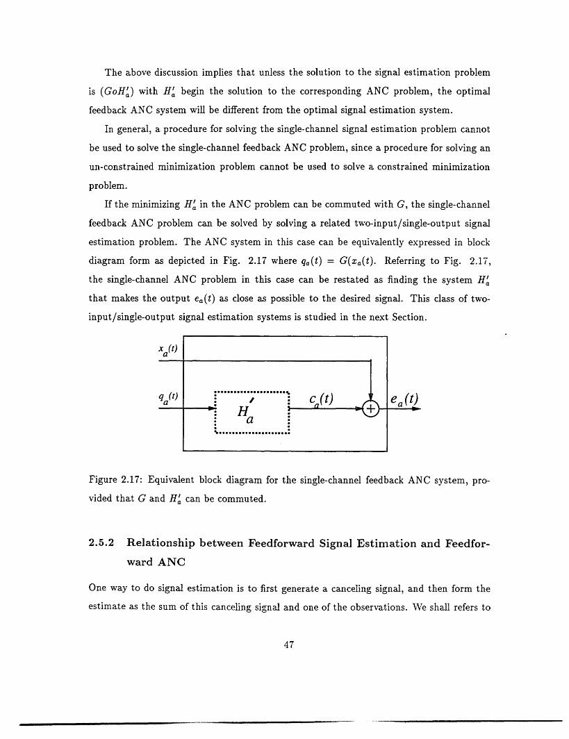
If the minimizing H' in the ANC problem can be commuted with G, the single-channel
feedback ANC problem can be solved by solving a related two-input/single-output signal
estimation problem. The ANC system in this case can be equivalently expressed in block
diagram form as depicted in Fig. 2.17 where qa(t) = G(xa(t). Referring to Fig. 2.17,
the single-channel ANC problem in this case can be restated as finding the system H'
that makes the output ea(t) as close as possible to the desired signal. This class of two-
input/single-output signal estimation systems is studied in the next Section.
Xa(t)
qa ) ea (
Figure 2.17: Equivalent block diagram for the single-channel feedback ANC system, pro-
vided that G and H' can be commuted.
2.5.2 Relationship between Feedforward Signal Estimation and Feedfor-
ward ANC
One way to do signal estimation is to first generate a canceling signal, and then form the
estimate as the sum of this canceling signal and one of the observations. We shall refers to
47
.......... ......... c ) H a
%............

this approach as feedforward signal estimation.
Figure 2.18: Feedforward signal estimation system.
A generic block diagram for a single-channel feedforward signal estimation system is
depicted in Fig. 2.18. As depicted in Fig. 2.18, this system is a two-input/single-output
system in which the output es(t) is the sum of the canceling signal cs(t) and the input signal
xs(t). Moreover, the canceling signal is generated solely based on one of the inputs, namely
qs (t).
The adaptive noise canceling system proposed by B. Widrow [52] has the same structure
as the system in Fig. 2.18, except that in Widrow's system Hs is continuously adjusted.
The objective of the feedforward signal estimation system is to make e(t) as close as
possible to some desired signal ds(t). Specifically, the feedforward signal estimation problem
can be stated as follows:
Find the single-input/single-output system Hs that minimizes
J ({[xs(r) + Hs(qs(r)), d(r)] : 0 < r < T}). (2.36)
Next, we consider the single-channel feedforward ANC system. As depicted in Fig.
2.19, a single-channel feedforward ANC system is a two-input/single-output system where
the output e(t) is generated as the sum of the canceling signal ca(t) and the input signal
xa(t). Moreover, the canceling signal ca(t) is generated as the output of system G, and it is
assumed that G is not an identity system. In this system, Xa(t) and c(t) are both physical
signals, and system G represents the effect of the transducer that physically generates the
canceling signal.
48

Figure 2.19: Feedforward ANC system.
The objective of the single-channel feedforward ANC system is to make e(t) as close
as possible to some desired signal da(t). Specifically, the feedforward ANC problem can be
stated as follows:
Find the single-input/single-output system Ha that minimizes
J ({[Xa(T) + (GoHa)(qa(r)), da(r)]: 0 < T < T}). (2.37)
Comparing the feedforward signal estimation problem to the feedforward ANC problem,
we see that the feedforward ANC problem can be viewed as a constrained version of the
feedforward signal estimation problem. Specifically, the feedforward ANC problem can be
stated as finding Hs that minimizes the expression in eq. (2.36) subject to the constraint
that Hs must be of the following form
H = GOHa, (2.38)
for a given system G and some system Ha.
We now compare the single-channel feedforward signal estimation system to the single-
channel feedforward ANC system in terms of their input/output characteristics. To this
end, we assume that both systems are driven by the same inputs and that the desired signal
for both systems is the same. We also assume that each system is designed so that the the
distance between its output and the desired signal is minimized.
49

Under these assumptions, the performance of the ANC system is never better than the
performance of the corresponding signal estimation system, since the optimal ANC system
is obtained by minimizing J(.) subject to a constraint, and the optimal signal estimation
system is obtained by minimizing J(.) without any constraints.
Again under these assumptions, if the minimizing Hs happens to equal (GoQ) for some
system Q, the optimal ANC system will be identical to the optimal signal estimation system.
Specifically in this case, the minimizing Ha in the ANC problem is system Q. For example,
if G is invertible, the minimizing Hs can be expressed as
= IoH. (2.39)
= Go(G'oH,). (2.40)
This implies that the solution to the feedforward ANC problem can be expressed in terms of
the solution to the corresponding feedforward signal estimation problem with Ha = G - 1oHs.
The above discussion implies that unless the solution to the signal estimation problem is
(GoHa) with H' being the solution to the corresponding ANC problem, the optimal ANC
system will be different from the optimal signal estimation system.
In general, a procedure for solving the feedforward signal estimation problem can not be
used to solve the feedforward ANC problem, since a procedure for solving an unconstrained
minimization problem cannot be used to solve a constrained minimization problem.
If the minimizing Ha in the ANC system can be commuted with G, the feedforward
ANC problem can be solved by solving a related feedforward signal estimation problem.
Specifically in this case, the minimizing Ha is the solution to the signal estimation problem
with xs(t) = Xa(t) and q(t) = G(qa(t)).
2.6 Summary
Acoustical principles behind ANC and several commonly used control strategies for ANC
were reviewed in this chapter. The relationship between active noise cancellation and signal
estimation was also explored.
Numerical studies were presented to demonstrate the feasibility of minimizing the total
50

acoustic potential energy in an enclosure. These studies showed that at low frequencies,
a few secondary sources can be used to obtain substantial reduction in the total acoustic
potential energy in an enclosure provided that two or three modes dominate the response
of the enclosure. In another study, it was found that driving the acoustic pressure to zero
at a single point in an enclosure produces a zone of quiet around this point which has a
diameter of about one tenth of the wavelength of the excitation frequency. It is important
to recall that the secondary source strengths in all these studies were calculated based on
the exact knowledge of the primary source strength for all time. However in a practical
ANC system, the primary source strength is unknown and must be estimated based on the
available measurements.
Existing control strategies for ANC were characterized as pointwise feedforward con-
trollers or as pointwise feedback controllers.
Feedforward systems achieve noise cancellation by exploiting the cross-correlation be-
tween the reference signal q(t) and the unwanted noise n(t) at the error microphone. For
the single-channel feedforward ANC system, we showed that the optimal, in the minimum
mean-square sense, canceling signal at the error microphone is the LLSE of -n(t) based on
p"(t) = q(t) * ga(t), (2.41)
where Gall(s) is the all-pass part of the transfer function from the input of the canceling
loudspeaker to the value of the canceling field at the location of the error microphone, see
equation (2.28). We also showed that this formulation can be used to compute the optimal
performance of the feedforward system based on the second-order statistics of {n(t), q(t)}.
Feedback systems achieve noise cancellation by exploiting the auto-correlation of the
noise n(t) at the error microphone. For the single-channel feedback ANC system, we showed
that the optimal canceling signal at the error microphone is the LLSE of -n(t) based on
p'(t) = n(t) * gall(t), (2.42)
where Gaui(s) is the all-pass part of the transfer function from the input of the canceling
loudspeaker to the output of value of the canceling field at the location of the error micro-
phone, see equation (2.26). We also showed that this formulation can be used to compute
51
- :
------- --- __ -
the optimal performance of the feedback system based on the second-order statistics of n(t).
Using the above analysis we can compare the optimal performance of the feedforward
system to the optimal performance of the feedback system. Based on this analysis, we
expect the feedforward system to achieve low levels of attenuation whenever the reference
signal is weakly correlated with the noise at the error microphone.
The main drawback of the feedforward systems is the problem of how to acquire a
reference signal that is highly correlated with the unwanted noise and at the same time
avoid acoustic feedback from the output of the canceling loudspeaker to the reference signal.
The main drawback of analog feedback systems is that these systems can not be tuned to
take advantage of the statistical characteristics of the unwanted noise. The main drawback
of the digital feedback system of Graupe [26] is that it can only be used when the transfer
function from the canceling loudspeaker to the error microphone contains no delay. This
severely limits the applications in which this system can be used. Furthermore, a multiple-
microphone version of the system proposed by Graupe does not exist.
In Section 2.5, we explored the relationship between signal estimation and active noise
cancellation. The systems studied in this Section were free to be linear or non-linear and the
cost functions involved were quite general. By structuring the signal estimation problem in a
particular way, we were able to illustrate the close relationship between single-channel signal
estimation and single-channel feedback active noise cancellation and the close relationship
between feedforward signal estimation and and feedforward active noise cancellation. In
each case, we showed that the active noise cancellation problem can be viewed as a con-
strained version of the signal estimation problem.
In the context of pointwise active noise cancellation, our goal is to develop a general
framework for designing feedback active noise cancellation systems that can be used in a
wide range of applications. Our formulation can be used in single-microphone as well as
multiple-microphone configuration, and the resulting algorithms will take advantage of the
the statistical characteristics of the unwanted noise.
We will then extend the above framework to the case where the performance criterion
is distributed. The performance criterion in this case is the total acoustic energy in an
52

enclosure. However, the measurements are still made using ordinary microphones, and the
control signal is still used to drive an ordinary loudspeaker. Most importantly, the control
signals are generated causally based only on the outputs of the microphones.
53

Chapter 3
Pointwise Optimal Feedback
Control for ANC
3.1 Introduction
In this chapter we develop an optimal feedback controller for attenuating the acoustic pres-
sure at the locations of a finite number of error microphones. Our controller is designed to
achieve the same acoustic objective as the multiple-channel feedforward controller in [18];
however, our controller generates the control signal based on the outputs of the error micro-
phones, and not based on a separate reference signal. Therefore, the feedback ANC system
developed in this chapter achieves the same acoustic objective as the feedforward ANC
system in [18], without the problems associated with acquiring an appropriate reference
signal.
An important feature of the optimal feedback controller is that it takes full advantage
of the statistics of the noise. LMS-type feedforward controllers used in ANC systems take
advantage of the statistical characteristics of the noise to be canceled. However, existing
feedback ANC controllers do not take advantage of the noise statistics (except under very
restrictive assumptions [26]).
We present a procedure for designing optimal feedback controllers for pointwise ANC
that can be used under very general conditions. The error microphones are placed at those
54
locations where noise attenuation is desired, and the canceling loudspeaker is placed in
the vicinity of these microphones. Given a specific arrangement of the error microphones
and the canceling loudspeaker, and given a specific statistical model for the noise at these
microphones, our design procedure determines the optimal feedback controller. Specifically,
our design procedure finds the controller that minimizes a performance criterion involving
the mean-square sum of the residual signals at the error microphones and the mean-square
sum of the control signal.
Our approach is to model the residual signals at the microphones as the sum of the
outputs of two linear system. The unwanted noise signals at the microphones are modeled
as the outputs of a multiple-input/multiple-output linear system driven by a white process.
Similarly, the canceling signals at the microphones are modeled as the outputs of a single-
input/multiple-output linear system driven by the control signal. Finally, the residual
signals at the microphones are modeled as the sum of the outputs of these two linear systems.
We show that the control signal that minimizes a certain class of pointwise performance
criteria is a linear feedback of the estimated states of these two linear systems. These
state estimates are computed using a Kalman filter, and the feedback gain is computed by
iterating a Riccati equation. The single-microphone case is presented first, and the results
are then extended to the multiple-microphone case.
In Section 3.4, we show that the optimal feedback controller developed in this chapter
can be thought of as a generalization of the optimal feedforward controller. Specifically,
the optimal feedforward controller generates the canceling signal based on all the available
measurement, but the optimal feedforward controller generates the canceling signal based
on a proper subset of the available measurements.
The control algorithms developed in this chapter are discrete-time algorithms. Unless
stated otherwise, we assume throughout this chapter that the noise to be attenuated, the
canceling signal, and all other intermediate signals are appropriately sampled. Unless stated
otherwise, throughout this chapter "t" represents the normalized sampling time.
55
3.2 Single-Microphone Optimal Feedback Controller for ANC
A single-microphone optimal feedback controller for ANC is developed in this Section. The
system utilizes one error microphone and one canceling loudspeaker. The microphone is
placed at the point where noise attenuation is desired, and the loudspeaker is placed as
close as possible to this microphone. The acoustic objective is to attenuate the pressure at
the location of the microphone. The loudspeaker produces a secondary field that interferes
destructively with the primary field at the microphone, generating a zone of quiet around
the microphone as reported in [15].
A generic single-microphone feedback ANC system is depicted in Fig. 3.1 where m(t) is
the microphone output, and r(t) is the input of the canceling loudspeaker. The microphone
measures the sum of the unwanted noise n(t) and the canceling signal c(t). The objective
is to generate r(t), based on the measurements of m(t), so that the power of the residual
signal at the microphone is minimized.
Throughout this chapter we rely on the following model for the microphone. The output
of the microphone is assumed to be the sum of the acoustic pressure at the location of
the microphone and the microphone measurement noise. According to this model, the
only distortion introduced by the microphone is this additive measurement noise. This
microphone model is quite accurate for most practical pressure microphones at frequencies
below 1000Hz [6].
The block diagram for the single-microphone ANC system that we propose and develop
in this Section is depicted in Fig. 3.2. The system G(z) represents the overall transfer
function from the canceling loudspeaker input r(t) to the value of the canceling field at the
location of the microphone c(t) and incorporates the transfer function for the loudspeaker
and the propagation path between the loudspeaker and the microphone. The microphone
output m(t) is the sum of the unwanted noise n(t), the canceling signal c(t), and the
microphone measurement noise v(t).
Our basic strategy for solving the ANC problem is to view this problem as a stochastic
optimal control problem with n(t) being the stochastic disturbance and G(z) being the plant.
From this point of view, the objective is to keep the output of the plant, e(t) = c(t) + n(t),
56

as close to zero as possible. Note that e(t) is the value of the residual acoustic field at the
location of the microphone, i.e. the sum of the noise field at the location of the microphone
and canceling field at the location of the microphone.
Noise SourceIt,
/
K> ~ c(t)
Error Microphone
m(t)
"I-,\~~~~~~~~~ ~Cancelling Loudspeaker
r(t)
.............................. ll~&l (......
Figure 3.1: Generic single-microphone feedback active noise cancellation system.
3.2.1 Model Specification
The stochastic optimal control formulation requires a disturbance model and a plant model.
We model the noise n(t) as the output of a pole-zero system function driven by a white
process:q i
n(t) = akn(t - k) + ,/3kw(t - k) j < q, (3.1)k=l k=l
where w(t) is a zero mean unit variance white Gaussian process, i.e. n(t) is modeled as an
ARMA process. The plant model, corresponding to the transfer function from the input
of the canceling loudspeaker to the value of the canceling field at location of the error
microphone, is the pole-zero system function
-1 bk Z -kG(z) -17- - m < n. (3.2)1 + ;=- akz k m<n
57
-
r-
...............I'll ...
-A1Z.-H- 1, -
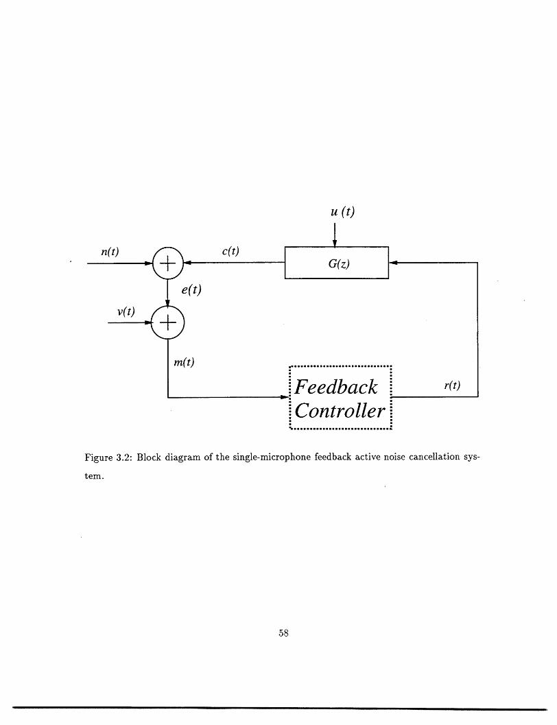
u (t)
n(t) c(t) - - -- -- ___ I .1' / I I _
m(t) .................................
m. ee acd) ~(t._Feedback r(t)
.Controller.................................
Figure 3.2: Block diagram of the single-microphone feedback active noise cancellation sys-
tem.
58
__1 LY(Z) I -
e(t)
VW
.

We represent the system of Fig. 3.2 in state-space form in three steps. First we will
derive a state-space representation for the disturbance model eq. (3.1), and then we will
derive a state-space representation for the plant model eq. (3.2). These two representations
are finally combined to get the overall state-space representation for the system in Fig. 3.2.
The disturbance model can be expressed in state-space form as [34, 3, 2].
Xd(t) = d Xd(t - 1) + Ld W(t- 1)
n(t) = d Xd(t),
(3.3)
(3.4)
where xd(t) is the (q x 1)
(q x q) transition matrix
state vector for the disturbance model; 4Id is the corresponding
-al 1 0 ...- 0
-- O2 0 -.
0
0
(3.5)
Ld is the (q x 1) vector
Ld = [ 1 ... j ... o];
and Hd is the (1 x q) unit vector
Hd = [10...0].
Similarly, the plant model can be expressed in state-space form as [34]:
xp(t) = Jp x(t- 1) + Gp (t- 1)+ Lp u(t -1)
c(t) = Hp xp(t),
where xp(t) is the (n x 1) state vector for the plant model;
random variables such that
u(t) is an (n x 1) vector of
E {U(t)u(r)T} = b(t - )Inxnn
59
(3.6)
(3.7)
-- -
-Oq

with u(t) independent of w(t); Dp is the (n x n) transition matrix of the plant
-al 1 0 ..- 0
-a 2 0 -.
: : *..
-an 1 0 ...... 1
-an 0 ...... 0
(3.8)
Gp is the (n x 1) vector
Gp = [bl * bm 0 0 ]T;
Lp is the (n x n) matrix
Lp = uInxn;
and Hp is the (n x 1) unit vector
Hp = [1 0 ... o0]T.
The state-space model for the overall system is now obtained by combining (3.3-3.4)
with (3.6-3.7):
x(t)
m(t)
= x(t-1)+Gr(t-1)+L
= Hx(t) + v(t),[
w(t- 1)
u(t- 1) J (3.9)
(3.10)
where x(t) is the state vector of the overall system
x(t) = Xd(t)
Xp(t)
( is the corresponding (q + n) x (q + n) transition matrix
)=[
(3.11)
(3.12)0d 0
0 c:P J
60
41DP =

G is the (q + n) x 1 vector
0
0
GP
~~~~; ~(3.13)
L is the (q + n) x (q + n) matrix
[Ld 01L=
0 Lp
and H is the 1 x (q + n) vector
H = [Hd Hp].
The measurement noise in the error microphone is modeled by the white Gaussian process
v(t) whose variance is a., and v(t) is independent of w(t) and u(t).
3.2.2 The Optimal Feedback Controller
The goal of the ANC system is to choose {r(t) t = 0,..., N - 1} so that the following
performance measure is minimized:(N-1
J(N) = E { {e2(t) + p r2(t)} + e2(N) . (3.14)t=O
To be causally realizable, the choice for r(t) must be a function of the available measure-
ments at time "t", i.e. it must be a function of {m(r) : r < t - 1}. The first summand in
(3.14) represents the power of the residual signal at the microphone, and the second sum-
mand represents the power expended by the control signal. Here, p is a weighting factor
which is chosen to achieve a trade off between control effort and noise attenuation. Recalling
that
e(t) = H x(t), (3.15)
we can rewrite J(N) in terms of the state vector x(t) as
N-1 J(N) = E {xT(t)HTHx(t) + p r2(t)} + T(N)HTHx(N) ' (3.16)
t=O
61
G =

It is important to observe that (3.16) is the expected value of a quadratic function of the
state vector x(t) and the control signal r(t). Following standard terminology from control
literature, we shall refer to this minimization problem as the "Finite Horizon Optimal Linear
Quadratic Control Problem".
Since the performance measure J(N) is the expected value of a quadratic form in the
state and the control, the minimizing choice for {r(t): t = 0, . . ., N - 1} is a linear feedback
of the optimal state estimates [24]. The optimal state estimates can be computed using
a Kalman filter, and the feedback gain can be computed by iterating a Riccati difference
equation. To this end, let us denote by
i(tjt) = E{x(t)jm(1),...,m(t)} (3.17)
the state estimate based on observations up to time "t", and by
P(tlt) = E {[x(tt)- x(t)][&(tjt) - (t)]TIm(1), ... ,m(t)} (3.18)
the associated error covariance matrix.
Then using the standard Kalman filter formulation, i(tjt) and P(tit) can be computed
sequentially in time, in two stages, as follows:
Propagation Equations:
:(tit -i1) = 5:(t - 1lt - 1) + G u(t - 1) (3.19)
P(tlt-1) = P(t-It-1)T + L LT (3.20)
Updating Equations:
&(tt) = &i(tlt- 1) + Kf(t)[m(t)- H i(tlt- 1)] (3.21)
P(tlt) = [I- Kf(t) H]P(tlt - 1), (3.22)
where Kf(t) is the Kalman gain given by
1Kf (t) = HP(tlt - 1)HT + ,2 P(tlt- 1)HT. (3.23)
The minimizing choice for {r(t): t = 0,...,N -1} is then given by
r(N-j) = -[GP(j-1)G + p]-lGTP(j 1) x(N - jIN-j) j= 1,...,N
= Kc(j- 1) (N-jlN - j), (3.24)
62

where the (m + n) x (m + n) matrix P(j) is obtained by iterating the following Riccati
difference equation:
P(j + 1) = bTp(j)4 _ bTp(j)G[GTp(j)G + p]-lGTP(j) + HTH, (3.25)
with the initial condition P(O) = H T H . The resulting minimum value of the
index J(N) can also be computed based on P(N) [35]. The block diagram for
ANC system is depicted in Figure 3.3.
performance
the resulting
Optimal Feedback Controller........................................................................Optimal Feedback Controller
Figure 3.3: Block diagram of our single-microphone feedback ANC system.
Infinite Horizon Case
If we consider the above problem with both time-invariant system matrices and with con-
stant weighting factor p, and if we allow N to approach infinity, a new performance index
63

can be defined as
J= lim -J(N)N-oo N
In this case, we ask for the choice of {r(t) : t = 0,1,...} that minimizes J. This is a well
posed problem provided that [, G] is stabilizable, and [, H] is detectable. In this case,
P(j) converges to a constant matrix P(oo) which is the unique positive definite solution of
the following algebraic Riccati equation
P(oo) = Tp( 0 )p -_ TP(oo)G[GTP(o)G + p]-lGTP(oo) + HTH. (3.26)
In this case, the minimizing choice for r(t) is given by
r(t) = -[GTP(oo)G + p]-GTP(oo)b i(tlt) (3.27)
= K,(oo) i(tjt). (3.28)
Note that the control gain, Kc(oo), is time-invariant.
Similarly, the error covariance matrix, P(tlt- 1) in the Kalman filter, converges to
a constant matrix P(oo) which is the unique positive definite solution of the following
algebraic Riccati equation
P(oo) = IP(oo)(DT - P(oo)HT[HP(oo)HT + U2]-lHp(x)T + LLT,
provided that [, L] is stabilizable and [, H] is detectable. The Kalman filter equations
reduce to:
Propagation Equation:
i(tt - 1) = ~ :i(t - 1t - 1) + G u(t - 1) (3.29)
Updating Equation:
5i(tlt) = 5i(tjt - 1) + Kf(oo)[m(t) - H 5i(tt - 1)], (3.30)
where Kf(oo) is the Kalman gain given by
1Kf(oo) = HP ) +2p(oo)HT + 2 P()H (3.31)
V
Note that the Kalman filter in this case is linear and time-invariant. Recalling that the
control gain Kc(oc) is also time-invariant, we conclude that the controller becomes a linear
time-invariant system in this case.
64

3.2.3 Frequency-Domain Perspective
Our formulation of the ANC problem so far has been entirely in the time domain. Addi-
tional insight can be gained by looking at the closed-loop ANC system in the frequency
domain. For this purpose, we shall concentrate on the infinite horizon case in which the
overall system is linear and time-invariant, and all the signals involved are jointly station-
ary. Furthermore, we assume that the objective is to minimize the pressure fluctuations at
the error microphone, i.e. we assume that the weighting factor for control effort, p in eq.
(3.14), is zero.
Let H(z) denote the transfer function of the controller in Fig. 3.3. Since the measure-
ment noise v(t) is white and G(z) contains at least one delay, the causal controller that
minimizes E{m2 (t)} is the same as the causal controller that minimizes E{e2 (t)} (note
that m(t) = e(t) + v(t)). Therefore, we can characterize the optimal feedback controller as
the controller that minimizes E{m2(t)} in Fig. 3.3. Referring to this figure, we define the
closed-loop transfer function T(z) as
1
1 - H(z) G(z) (3.32)
, and we define z(t) as
z(t) = n(t) + v(t). (3.33)
The power spectrum of the microphone output Pmm(e3w) can be expressed in terms of
the power spectrum of z(t), i.e.
Pmm(e3w) = T(eiw) 2 Pzz(eJw)(3.34)
Equations (3.32)-(3.34) show how the controller H(ejw) affects the power spectrum of
the microphone output. To minimize the variance of m(t) or equivalently to minimize
the variance of e(t), we need to make IT(eJw)i small over those frequencies for which the
unwanted noise has significant power. This is precisely what the optimal controller does.
Specifically, the optimal controller uses the noise model to determine those frequencies
for which the unwanted noise signal has significant power, and it chooses H(z) so that
the magnitude of the resulting closed-loop transfer function, T(e3w)j, is small over these
65
frequencies. From this point of view, it is clear that the more narrow-band the spectrum of
n(t), the higher the attenuation level achieved by the feedback controller. An example of
this will be presented in the next section.
Having a good model for the unwanted noise is crucial for achieving high attenuation
levels. In the absence of an accurate model for the the unwanted noise (i.e. without
knowing at which frequencies the power of the unwanted noise is concentrated), one is
forced to assume that the spectrum of the noise is flat over a wide range of frequencies.
This results in an ANC system with low attenuation over a wide range of frequencies (e.g.,
noise canceling headphones developed by Wheeler [51]). On the other hand, in cases for
which the unwanted noise is relatively narrow band and the noise is well modeled, the active
noise cancellation system can be designed to achieve very high attenuation levels. This is
done by choosing the controller such that the closed-loop system has high attenuation over
the narrow band of frequencies where the power of the noise is concentrated.
Analysis of the feedback controller in chapter 2 can also be used to explain why relatively
narrow band noise is highly attenuated by the optimal feedback controller. Recall that this
analysis was done in continuous time; hence, "t" represent the continuous time variable in
this paragraph. Referring to Fig. 2.3 of Chapter 2, it was shown that the optimal canceling
signal in the single-channel feedback ANC system is the LLSE of -n(t) based on
p'(t) = n(t) * gal1(t), (3.35)
where Gall(s) is the all-pass part of G(s). The mean-square estimation error will be small
whenever n(t) can be estimated accurately based on p'(t). For a relatively narrow band
n(t), Gall(s) can be approximated as a delay. Therefore in the narrow band case, the
problem reduces to predicting n(t) based on p'(t) = n(t - T), where Tr is the delay. More
importantly, the mean-square estimation error will be small with a narrow band n(t), since
a narrow band signal is highly predictable.
3.2.4 Frequency-Weighted Optimal Controller for ANC
Assuming time-invariant system matrices and stationary acoustic noise, we shall drive a
feedback controller that minimizes a cost function involving the frequency-weighted power
66

of the residual signal at the microphone. Referring to Fig. 3.2, the objective in this section
is to minimizejN-1 A
- ,iN E E (eE2w(t) + p r2(t) + e2() , (3.36)
where ew(t) = e(t) * s(t), with s(t) being a pre-specified weighting filter. The relationship
between e(t) and e(t) can be expressed in state-space form as:
Xw(t) = ,w xw(t - 1) + Gwe(t) (3.37)
ew(t) = Hw x(t). (3.38)
The weighting filter s(t) might represent the perceived loudness of sound at different
frequencies. In this context, the filter s(t) is typically referred to as an A-weight filter.
The state-space representation eqs. (3.37)-(3.38) of the weighting filter can be combined
with the state-space representation eqs. (3.9)-(3.10) of the original acoustic system. The
state-space representation for the combined system is
xc(t) = 1'c x(t-1) + Gc r(t-1) + Lc (t -1) (3.39)u(t-1) J
m(t) = H, x(t) + v(t), (3.40)
where xm(t) is the state vector of the combined system
(t)1x(t)= (t) (3.41)
LW(t)
· , is the corresponding transition matrix
'P 0c= [0; (3.42)
GwH wJ
Gc is the column vector
Gc = G ; (3.43)
o
67

Lc is the matrix
LL = (3.44)
and Hc is the row vector
H = [H o]. (3.45)
Next, we express the performance criterion JO in terms of the state vector x:(t). For
this purpose, we define
{N-1 3
J(N) = E {tZ (e2 (t) + p r2(t)) + e2 (N)}. (3.46)kt=0
Recalling that
ew(t) = [o Hw] xc(t), (3.47)
we can rewrite J(N) in terms of the state vector xc(t) as
N-1A
J(N) = E (xT(t)CTC* xc(t) + p r2(t)) + XT(N)CTC*xc~(N) (3.48)t=O
where C, = [o Hw]. Note that J(N) is the expected value of a quadratic function of the
state vector xc(t) and the control signal r(t).
Since J = limN, Mo1 J(N), the choice of {r(t): t > O} that minimizes J is a linear
feedback of the optimal state estimates of the combined system, provided that [c, Gc] is
stabilizable and [, H] is detectable. The exact equations for the controller are obtained
following steps identical to the ones followed to get the infinite horizon controller in Section
3.2.2.
3.2.5 Implementation and Performance of the Optimal Feedback Con-
troller
Two sets of experiments were performed to evaluate the performance of the optimal single-
microphone feedback ANC system. In the first set, computer simulations on recorded
aircraft noise were used to compare the performance of the optimal feedback system to the
performance of the feedforward system proposed in [10]. The second set of experiments
68

were carried out to measure the performance of the hardware implementation of the op-
timal feedback system in the context of aircraft noise. The performance of the hardware
implementation of the optimal feedback system was also compared to the performance of a
commercial analog feedback system built by the BOSE Corporation.
Our feedback system and the feedforward system in [10] were evaluated using a set of
noise canceling headphones. These headphones were equipped with a reference microphone,
an error microphone, and a canceling loudspeaker. The reference signal for the feedforward
controller was obtained as the output of the reference microphone that was attached to the
outside of the headphones, and the error microphone was placed inside the headphones. The
canceling loudspeaker was also placed inside the headphones, about 1.2 centimeters away
from the error microphone. In this case, the transfer function G(z) of Figure 3.2 corresponds
to the transfer function from the canceling loudspeaker to the error microphone inside the
headphones.
A separate set of experiments was performed initially to estimate the transfer function
G(z) and the coefficients of the disturbance model. It was found that an ARMA model with
three zeros and four poles produces a very good approximation to the transfer function from
the canceling loudspeaker to the error microphone. The disturbance model was an all-pole
system function of order four, and the coefficients of this model (s in (3.1)) were estimated
using the algorithm in [40]. All the controllers discussed in this section are designed based
on this estimated plant model and this estimated disturbance model.
Simulations
The performance of the feedforward system of Burgess [10] was compared to the perfor-
mance of the infinite horizon feedback controller developed in Section 3.2.2. In computer
simulations, the feedforward system of Burgess was able to attenuate the noise generated by
a propeller aircraft by about 17dB. This result was obtained with a 350-tap finite impulse
response controller and using recordings of the noise made at the reference microphone and
at the error microphone. The sampling rate was 6KHz. Using the same recorded noise
at the error microphone, our infinite horizon feedback controller was able to attenuate the
69
---

noise power at the error microphone by about 26dB. Referring to Fig. 3.2, this attenuation
was calculated according to the following equation:
E~e2(t)} (.9Un-Weighted Attenuation = 10 log E 2(t)} (3.49)
The feedforward controller and the feedback controller were designed based on the exact
knowledge of the plant model and the disturbance model. The power spectrum of the
unwanted noise and the power spectrum of the residual signal obtained with the infinite
horizon feedback controller are depicted in Fig. 3.4(a).
Another set of simulations was performed to illustrate the performance of the frequency-
weighted optimal feedback controller. Again, we used the same propeller aircraft noise that
was used in the simulations described in the previous paragraph. The frequency response
of the weighting filter, s(t), that was used in the design of the controller is depicted in Fig.
3.5. This filter models the variations in perceived loudness of sound at different frequencies.
According to this model, a pure tone of unit power at KHz sounds 70dB louder than a pure
tone of unit power at 10Hz. The power spectrum of the unwanted noise at the microphone
and the power spectrum of the residual signal obtained with the frequency-weighted optimal
feedback controller are depicted in Fig. 3.4(b). The un-weighted attenuation in this case is
about 20dB. Referring to Fig. 3.2, let us define the weighted attenuation as
E{,e2(t)}Weighted Attenuation = 10 log10 E{(t)}, (3.50)
where e(t) = e(t) * s(t) and n(t) = n(t) * s(t). The weighted attenuation in this case
is about 16dB. For comparison, the weighted attenuation corresponding to Fig. 3.4(a) is
about 11dB. We see that incorporation of the weighting filter in the design of the feedback
controller improves the weighted attenuation by about 5dB.
Hardware Implementation
The infinite horizon feedback controller, designed without frequency weighting, was imple-
mented in hardware using a single AT&T DSP32C chip with 6KHz sampling rate. The
resulting noise canceling headphones were placed in an enclosure, and propeller aircraft
70

noise was injected into this enclosure. The headphones were able to attenuate the noise
power at the error microphone by 25dB.
The spectrum of the unwanted noise at the output of the error microphone and the
spectrum of the attenuated noise at the output of the error microphone obtained with our
feedback controller are depicted in Fig. 3.6(a). The closed-loop transfer function realized
by our controller, T(eJw), is depicted in Fig. 3.6(b). As expected from the discussion in
Section 3.2.3, the closed-loop system has high attenuation over the 90Hz-130Hz band where
most of the power of the unwanted noise signal is concentrated.
In Figure 3.7, the performance of our optimal feedback controller is compared to that
of the analog feedback controller developed commercially by BOSE Corporation. The spec-
trum of the original noise at output of the error microphone is depicted in Fig. 3.7(a). The
spectrum of the attenuated noise at the output of the error microphone obtained with our
controller and the spectrum of the attenuated noise at the output of the error microphone
obtained with the analog controller are depicted in Fig. 3.7(b). The overall attenuation ob-
tained with the analog feedback system is 17dB, and the overall attenuation obtained with
the optimal feedback system is 25dB. Looking at Fig. 3.7, we see that the optimal feedback
controller achieves higher attenuation than the analog controller over the 90Hz-130Hz band
where most of the energy of the unwanted noise is concentrated. On the other hand, the
optimal feedback controller achieves lower attenuation than the analog controller over the
350Hz-700Hz band where the original noise does not have significant power.
The main drawback of the above formulation is that the disturbance model and the
plant model must be known before the optimal controller can be computed.
3.3 Multiple-Microphone Optimal Feedback Controller for
ANC
In this section, the optimal control framework of Section 3.2 is extended to develop a feed-
back controller for attenuating the noise at the locations of "I" error microphones. The error
microphones are placed where noise cancellation is desired, and the canceling loudspeaker
71
-

Power Spectrum
Frequency (Hertz)
(a) Power spectrum of the propeller aircraft noise at the error microphone obtained using a feedback
controller designed without a weighting filter.
a
Power Spectrum90 C
I I I I ,
11 I I I I I
I I I II80 - ----- --------.-------- -------- --- ---- --------11 1 1 I t I11 1 1 1 I I
I T I I I t III I I I I I
70 -- .. ' - -------- r -.--- r -------- -------I \ ~ ,| ,Original Noie
60 -- -- ------------- - -I- -- -
|1 ' | g~~~~Residual with ANC
so t ' ------ r--------Ig'-- '40 ___ _ __I I ,I I I
I I I I I60 - ;--- -- - --------- ..... ....
20I I I I . II I I I
0 500 1000 1500Frequency (Hertz)
2000 2500 3000
(b) Power spectrum of the proper aircraft noise at the error microphone obtained
weighted feedback controller.
Figure 3.4: Results of our computer simulations.
with a frequency-
72

Weighting Filter4-
-u10 ° 101 102 103 104
Frequency(Hz)
Figure 3.5: Frequency response of the weighting filter.
73
lU
0
-10
-20
m' -306'aC
)-40
-50
-60
-70
on
, ,,,r .,, ,,n .r~ - r rr- -rUl
I-4- -- 4--I-- -- 4 - 4- --- 4---- - 44 4- 4-- - - -4- - -4 - -44~--
rT-rrrri -r rTTrn - r-r-IrT rl-- T- lirr
I I I I 111111 1 1 1 1 1 I I I I I 1I1111 I 1 1 111I 1111111 I I I I I Hl I I I1 I I
I I I I I 11 11 1 1 11 I I I I I I 11 1111 1 11 1 i ~-~~1 |~1~1 r~l' -- r-,-i ' [''-| -i1~ '-'t,111 1 I I i lll I , 11XI 1
l~~~~~~~~~~ I ~, I I Ill III lll |/ 111 I 11
I I I I I I II I I I I I I I I I / I I I I I| II I I I I
Ii I I I 1 1I 11 I 1 I 1 1 1I 1 11 1 I I I II1 1 1 11 I III i I I I 1111I 1 1 1 1 1 1111/ I I I I I IIII 1 1 I I I ill
I I I I I 1111 I 1i I It I I~ I I I I I III I I I I 1 I lII~-~-,- - r-~---l ~--~- T ~ -r-- r--~- ~-r ~ ~~---T- -T-- ~ II I I I I III I 1 i I I I 111 I I I i I 1111 I I I I I l
I I I I I I I II I I I I I/ 1I 1 1 1 1 1 1 1 ! 1 I I 1 I 1I III I I I 1 I 111 1 I I 1 111 I I I I I IIII I I I I I I II___-l_ LL-L___ L--_--,lLU, ,_-L-- L-l~- l,,_-----J-l-J-L
I I I I I 111 i I / 1 I111 II 1 I I II I I I I tI I I I / iI I I I I I I I I I I I I1 i I I I I I I I I
I I I I IlI 11 I t/ I III I 11 I 1 1! 1 1 1 I1 I I I 11 11| .~~~~~ I 11 1 1/1 1I 1 lill I I I I 1 11 1 1 I I I I Il... I+~,.___ + ----F~--t-- Ftlltt---e-- ++H----~+t+--H-+-~ It
l I I i t 1111 1 / I I I 1111 i I I I ! l 1 i I i I 11I I I II I 1 /1 1I 1 I II1 1 I I 1 I1 I II I 1 I tII
Ii I I I I I / I I I I I 111 I I ! ! ! ! 111 I i I 1. I I11
II I I I I I11 ./1 I 1I I 1 I1 Il l I _lL l/ L! _ 1111 _ 1 I' I 1 1Il
... li- I I llll11 / I | | | |W11 l I~ ~~~ ~ ~ I I Il l I i1 I I I I! l ! 11 I I ll I
II I I I 1IIIII /I I I I III I I t I!!! ! I I I IIIII I I I!1 111/ 1 I I I 111 IIl I I I 11! ! I I I I I111
~~~~I ~--- -'-'~---r-~-"rn-~--rn-Itl-'--~n~~~~~I I I III I 111 1 1 111ll I I I I!1111 I I I I 1I 1I I I I IIII / I I I i II1 I i I II ! 111 I I 11i
I I I I II I I 11 I I 1 II I I I 11 ! !! 1 I I 111 II
II I I I II I I !ll ! 1 1111 I § I I I III I I I I , I III
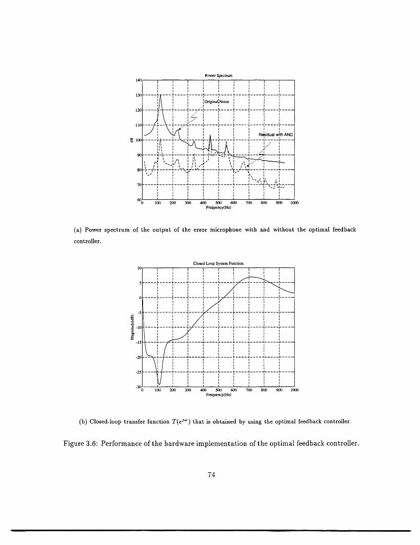
Power Spectrum140 I 1 1 1 1 1 1 I
I I I [ I I
I 1 1 I I I
130. ---- -. . .... - .. . . . . -
0riginaliNoise/1 I~~
I~ I I / tI I I I I I120 I I I I - I I I
l\ , ,~/11I) -- r--, -- IT ----
a I RtRdual with ANCI I- -I I I I I -
f J i I l' I \ I t I I- / , , , I , I I
I I I I I.
9( - ---- - -I ., I-,
I f I I I I II~~ ~ ~ ~ ~ ~ ~~~ a ei a wst ANI I . I I I I I I I'J i ! - . -!i, , I 4;J, -.. -'- --'*-- - -- --. - ---,- '=- .. =- - -- - ------ --- . . ..
0 I(X) 2(X) 3(X) 4(X) 5(X) 6(X) 7(X) 8(X) 9(X) I(X)Frequency(Hz)
(a) Power spectrum of the output of the error microphone with and without the optimal feedback
controller.
Closed Loop System Function
0 I--. ,-�-'-… L _ L,--I ---I -I -- --I - - -~~~~~I I I ' I % I I | |
· . %I I I 1 I _S I I ~ I I I
5 I…
a -( --1…-- - --15 …I
-20 … 4---4 -- - …--- n ~ ~ ~ ~ ~ ' ~ t I ; "I I '~ /'i I I
- ' - -- - - -- -- - --- --- -- - -- ---- --- -- --- -'~ / t ] 0 , 4 i I~ '~ i I--! I I ~ I I I I I) I I
25…F-t--___-____-_…__…_ I I I I I I I -~ ~ I, I
IX 2 3X) 4(X) 5(X) 6(X) 7X) 8X) 9(X) (XX)
Frequency(Hz)
(b) Closed-loop transfer function T(e)o that is obtained by using the optimal feedback controller.
Figure 3.6: Performance of the hardware implementation of the optimal feedback controller.
74I I I I I I I I I I
I I I I I I I I I\l I I I I I I I I II I I I I I I I I I
lI I I I I I I I [ I.... J. ... J ... .... ... .. ,' _ -L .... -... ... L _._._
IV I I I I I I I I
-3( t I I I I () I(X) 2(X) 3(X) 4(X) 5(X 6(X) 7(X) 8(X) 9(X)I I(XX
I I I I ~ I IrequIcy(Hz
(b) Close~-optasefnto @ . .... . ... obtaine . .. y .... r ...he-- .... ma feedbac conroler
Figure 3.6: Performance~ II of th hadwr imlmnaio of Ih opimlfebccotler
*~ I I /I I I I I4

Power Spectrum of the Original Noise
Frequency(Hz)
(a) Power spectrum of the propeller aircraft noise at the error microphone.
Power Spectrum of the Residuals115 I I i T [ I
/ I 1 1 I I I I I11 .... 1 1 1 1 1 1 1 1
.... I I I I I IAnalod Feedba:k Systei.,11 , , ,;, , ,' , ,
- .---- . ---.- L .. ... .....
) -- - - , I I /I I , I I ! I I,,~! II I I A / I I L ~ ~ ~ ~~I I I I Iz~'l~~~~~~~~~~~ ~~~~ ~ ~- ... -"T .-~ .-- --r --- - ...- -, ,- ..
i! I /! ! ! [, I , I Opimal Fetdback ystem
75 ---- -----.----- …------ 4.- - --- …--.--
I) ( 2(X) 3(8 4(X1 5(X) 6(X) 7(81 801) 9181) 1(88)Frequencey(Hz)
(b) Comparison of the analog feedback controller to the optimal feedback controller.
Figure 3.7: Performance of the hardware implementation of the optimal feedback controller./75 i t t 1i I N
I ti I [ , I I I I I ] I I/-I
6'l -, , -'' ~.- - -', 1"--'lc . -' . "r-", r..() I(X 2(X 3(X 4(X), 5(X ; (X 7(N 8(X 9(X I(XX) /
(b) Comparison/ of th analg fedbc cotole to the opIma Ifeebc IotrllI
Figure~ ~ ~~8, -3~-,-~~-'H-..- 3.
ntonf th .... ma ..... ac conroler
75
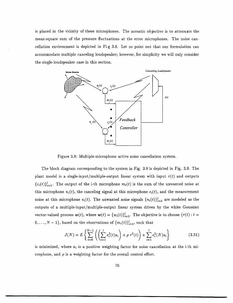
is placed in the vicinity of these microphones. The acoustic objective is to attenuate the
mean-square sum of the pressure fluctuations at the error microphones. The noise can-
cellation environment is depicted in Fi.g 3.8. Let us point out that our formulation can
accommodate multiple canceling loudspeaker; however, for simplicity we will only consider
the single-loudspeaker case in this section.
Noise Source Cancelling Loudspeaker
rft)
Figure 3.8: Multiple-microphone active noise cancellation system.
The block diagram corresponding to the system in Fig. 3.8 is depicted in Fig. 3.9. The
plant model is a single-input/multiple-output linear system with input r(t) and outputs
{ci(t)}i=. The output of the i-th microphone mi(t) is the sum of the unwanted noise at
this microphone ni(t), the canceling signal at this microphone ci(t), and the measurement
noise at this microphone v(t). The unwanted noise signals {ni(t)}li=l are modeled as the
outputs of a multiple-input/multiple-output linear system driven by the white Gaussian
vector-valued process w(t), where w(t) = {wi(t)}i=l. The objective is to choose {r(t) :t =
0,...,N - 1}, based on the observations of {mi(t)}i=l, such that
J(N) = E (( e(t)ai) + p r2(t) + ei(N)ai (3.51)Z ~~~~2t=O 2 i=1
is minimized, where ai is a positive weighting factor for noise cancellation at the i-th mi-
crophone, and p is a weighting factor for the overall control effort.
76
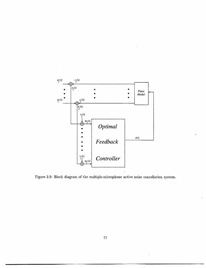
n (t)
nl(t) cl(t)
Figure 3.9: Block diagram of the multiple-microphone active noise cancellation system.
77

The unwanted noise signals at the microphones are modeled as the outputs of the
following linear system:
Xd(t) = IdX(t- 1) + Ldw(t- 1) (3.52)
n(t) = HdXd(t - 1), (3.53)
where n(t) is the (I x 1) vector of the unwanted noise signals
n(t) = [n, (t), n2(t), . . . , nl (t)]T;
Xd(t) is the state vector of this system, and the input of this system is the ( x 1) vector
w(t) with
E{W(t)w(-)T} = (t- ) I.
The plant model is the following single-input/multiple-output linear system with input
r(t) and outputs {ci(t)}=:
xp(t) = bp xp(t - 1) + Gp r(t - 1) + L p u(t - 1) (3.54)
c(t) = Hp xp(t - 1), (3.55)
where c(t) is the ( x 1) vector of the canceling signals at the microphones
C(t) = [Cl(t), C2(t), .. ,CI(t)]T;
xp(t) is the state vector of the plant model; and u(t) is the process noise representing the
unmodelled dynamics in the plant model with
E{u(t)u(r) T} = (t- r)I.
Following the same steps as the ones for the single-microphone case, we now derive the
state-space model for the overall system by combining (3.52-3.53) with (3.54-3.55):
x(t) = x z(t-1)+Gr(t-1)+L w(t - (3.56)
L u(t-1)
m(t) = H x(t) +v(t), (3.57)
78
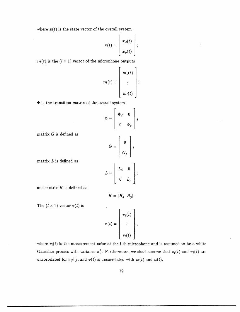
where x(t) is the state vector of the overall system
x (t) x ( t )
[x(t) Jmr(t) is the ( x 1) vector of the microphone outputs
ml(t)
m(t) = : m
ml(t)
4 is the transition matrix of the overall system
d 0]
0 (D
matrix G is defined as
GG=
matrix L is defined as
L = [Ld 01]0 Lp
and matrix H is defined as
H = [Hd H].
The ( x 1) vector v(t) is
v1(t)
v(t) = '
v(t)
where vi(t) is the measurement noise at the i-th microphone and is assumed to be a white
Gaussian process with variance a2. Furthermore, we shall assume that vi(t) and vj(t) are
uncorrelated for i 4 j, and v(t) is uncorrelated with w(t) and u(t).
79
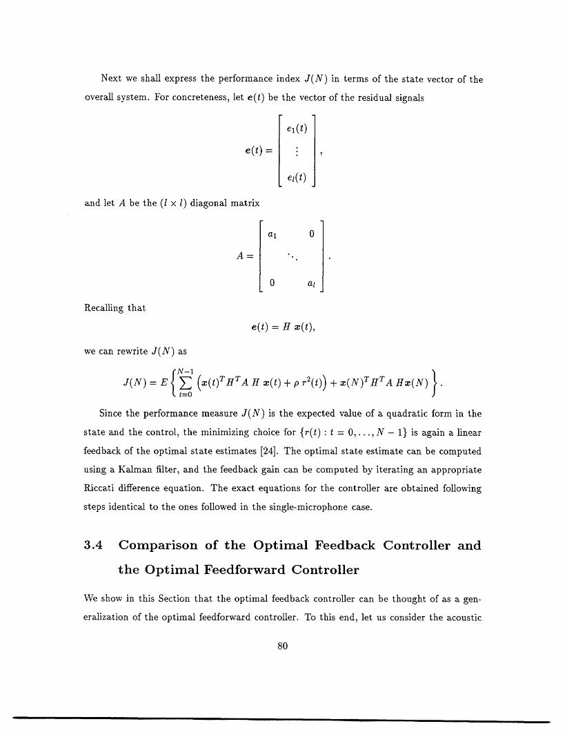
Next we shall express the performance index J(N) in terms of the state vector of the
overall system. For concreteness, let e(t) be the vector of the residual signals
e(t)
e(t) = . ,
el(t)
and let A be the ( x 1) diagonal matrix
al 0
A=
0 al
Recalling that
e(t) = H x(t),
we can rewrite J(N) as
{N-1
J(N) = E {: (x(t)THITA H x(t) + pr2(t)) + x(N)THTA Hx(N) .t=O
Since the performance measure J(N) is the expected value of a quadratic form in the
state and the control, the minimizing choice for {r(t): t = ,...,N - 1} is again a linear
feedback of the optimal state estimates [24]. The optimal state estimate can be computed
using a Kalman filter, and the feedback gain can be computed by iterating an appropriate
Riccati difference equation. The exact equations for the controller are obtained following
steps identical to the ones followed in the single-microphone case.
3.4 Comparison of the Optimal Feedback Controller and
the Optimal Feedforward Controller
We show in this Section that the optimal feedback controller can be thought of as a gen-
eralization of the optimal feedforward controller. To this end, let us consider the acoustic
80

environment depicted in Fig. 3.10. We assume that the desired acoustic objective is to
attenuate the pressure at Microphone 1 and that there is no feedback from the input r(t)
of the canceling loudspeaker r(t) to the output of Microphone 2. Furthermore, we assume
that the noise signals at the two microphones are jointly stationary. We will compare the
effect of using a two-microphone feedback controller to the effect of using a single-channel
feedforward controller for attenuating the acoustic pressure at Microphone 1. All signals in
this Section are continuous-time signals.
For compatibility with the analysis done in Chapter 1, we assume in this Section that
the output of each microphone is simply the value of the acoustic pressure at the location
of the microphone, i.e. we ignore the microphone measurement noise.
Canceling Loudspeaker
" (t Hn ()
Microphoi
n (t)2
r(t)
Microphone 2
n (t)2
Figure 3.10: Noise cancellation environment with one canceling loudspeaker and two mi-
crophones.
In Fig. 3.11, the two-microphone feedback controller H f b is used to attenuate the noise
at Microphone 1. The block diagram for this feedback system is depicted in Fig. 3.13,
where G(s) is the transfer function from the input r(t) of the canceling loudspeaker to the
canceling field at the location of Microphone 1. The output of Microphone 1, e(t), is the
sum of the noise at this microphone, n(t), and the canceling signal at this microphone
cl(t). There is no feedback from the input of the canceling loudspeaker to the output of
Microphone 2; hence, the output of Microphone 2 is simply the noise at this microphone
81

Canceling Loudspeaker
n (t)
Microphone
Microphone 2
c (t)I
Feedback Controller
Figure 3.11: Two-microphone feedback controller.
Canceling Loudspeaker
n (i
Microphone
Microphone 2
c (t)I
e(t)
r(t)
Feedforward Controller
Figure 3.12: Single-channel feedforward controller.
82
r(t)
r(t)
r(t)

n (t)1
elf
d
r(t)
HbH
Figure 3.13: Block diagram of the two-microphone feedback ANC system.
HjH
Figure 3.14: Restricted class of two-input/single-output controllers.
83
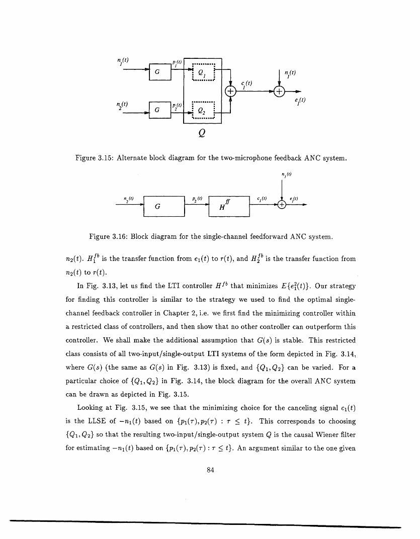
0)
Q
Figure 3.15: Alternate block diagram for the two-microphone feedback ANC system.
nI (t)
Figure 3.16: Block diagram for the single-channel feedforward ANC system.
n2(t). Hfb is the transfer function from el(t) to r(t), and Hfb is the transfer function from
n2(t) to r(t).
In Fig. 3.13, let us find the LTI controller Hfb that minimizes E{e2(t)}. Our strategy
for finding this controller is similar to the strategy we used to find the optimal single-
channel feedback controller in Chapter 2, i.e. we first find the minimizing controller within
a restricted class of controllers, and then show that no other controller can outperform this
controller. We shall make the additional assumption that G(s) is stable. This restricted
class consists of all two-input/single-output LTI systems of the form depicted in Fig. 3.14,
where G(s) (the same as G(s) in Fig. 3.13) is fixed, and {Q1,Q2} can be varied. For a
particular choice of {Ql, Q2} in Fig. 3.14, the block diagram for the overall ANC system
can be drawn as depicted in Fig. 3.15.
Looking at Fig. 3.15, we see that the minimizing choice for the canceling signal c1(t)
is the LLSE of -n 1 (t) based on {pl(7),p2() : r < t}. This corresponds to choosing
{Ql, Q2} so that the resulting two-input/single-output system Q is the causal Wiener filter
for estimating -ni(t) based on {pl(r),p2 (r) r < }. An argument similar to the one given
84

in Chapter 2 can be used to show that no other controller can outperform this controller
and that the optimal canceling signal at Microphone 1, cl(t) in Fig. 3.13, is unique.
In Fig. 3.12, a single-channel feedforward controller is used to attenuate the noise at
Microphone 1. The block diagram corresponding to this system is depicted in Fig. 3.16,
where G(s) is the transfer function from the input of the canceling loudspeaker r(t) to the
value of the canceling field at the location of Microphone 1. The output of Microphone
1, el(t), is the sum of the canceling signal at this microphone, c(t), and the noise at this
microphone nl(t). The reference signal for the feedforward controller is n2 (t), the output
of Microphone 2. The objective is to find the LTI controller H f f that minimizes E{el(t)}.
According to the analysis presented in Chapter 2 for the optimal single-channel feed-
forward controller, the LTI system Hff that minimizes E{e2(t)} in Fig. 3.16 is the causal
Wiener filter for estimating -nl(t) based on p2(t), where p2(t) = n 2 (t) *g(t). The resulting
canceling signal in this case is the LLSE of -nl(t) based on {P2(T) r <_ t}-
Based on the above analysis, we can now compare the optimal feedback controller to
the optimal feedforward controller. With the optimal two-microphone feedback controller,
the canceling signal at Microphone 1 is the LLSE of -nl(t) based on {pl(r),p2 (r) r _< t}-
With the optimal single-channel feedforward controller, the canceling signal at Microphone
1 is the LLSE of-nl(t) based on {p2(r) r t}. Therefore, with the optimal two-
microphone feedback controller the residual signal at Microphone 1 is the estimation error
in estimating nl(t) based on pi(t) and p2 (t); however, with the optimal single-channel feed-
forward controller the residual signal at Microphone is the estimation error in estimating
nl(t) based on p2(t) alone. In this sense, the optimal feedforward controller does not use
all the available measurements.
Let us note in passing that the optimal single-microphone feedback controller in this
case, using Microphone 1 only, will result in a canceling signal at Microphone that is the
LLSE of -ni(t) based on {pl(r) T r t} alone.
85
3.5 Summary
An optimal feedback controller for attenuating the acoustic pressure at a finite number of
microphones was developed in this chapter. The results in this chapter were based on the
following assumptions:
1. the unwanted noise signals at the microphones are modeled as the outputs of a known
linear system driven by a white process.
2. the canceling signals at the microphones are modeled as the outputs of another known
linear system driven by the control signal.
3. the residual signals at the microphones are modeled as the sum of the unwanted noise
signals and the canceling signals.
4. the observed signals are modeled as the sum of the residual signals and white mea-
surement noise, and this measurement noise is uncorrelated with all other processes
involved.
Given a stochastic model for the unwanted noise at the microphones and a linear sys-
tem model relating the canceling loudspeaker input of the outputs of the microphones, our
formulation can be used to determine the minimum achievable value of the statistical per-
formance criterion J which was defined in eq. (3.51). We also showed that our formulation
can be modified to minimize the frequency weighted power of the residual signal. More-
over, our formulation can be used to find the specific feedback controller that achieves this
minimum value.
The feedback controller developed in this chapter has a few advantages compared to
the existing feedback controllers. Recall that the analog feedback controller developed by
Wheeler [51] does not take advantage of the statistics of the noise. However, the feedback
controller developed in this chapter takes full advantage of the statistical characteristics
of the noise. The single-microphone feedback controller developed by Graupe [26] can not
be used in cases for which the plant model contains one or more delays. However, the
feedback controller developed in this chapter can be used in these cases. Furthermore, the
86

feedback controller developed in this chapter can be used in the single-microphone as well
as multiple-microphone configuration.
A comparison of the optimal feedback controller with the optimal feedforward controller
was presented in Section 3.4. We showed that both controllers generate the canceling signal
as the negative of the LLSE of the unwanted noise at the error microphone. However, the
feedback controller estimates the unwanted noise based on all the available measurements,
as opposed to the feedforward controller that estimates the unwanted noise based only on
the reference signal. In this sense, the optimal feedback controller can be thought of as a
generalization of the optimal feedforward controller.
The main drawback of the design procedure presented in this chapter is that the dis-
turbance model and the plant model must be known before the optimal controller can be
computed. The next chapter is devoted to the modeling of the unwanted noise based on
the measurements of this noise made by the microphones.
87

Chapter 4
Modeling of the Unwanted Noise
at a Single Microphone
4.1 Introduction
The design procedure of Chapter 3 is only useful if an algorithm for identifying the distur-
bance model and the plant model exists. The problem of identifying the disturbance model
in the single-microphone case is considered in this chapter. We assume that the unwanted
noise at the location of the microphone is a non-stationary autoregressive process and de-
velop a recursive/adaptive procedure for estimating the parameters of this process based
on the measurements made by the microphone.
An adaptive feedback ANC system can be obtained by combining the design procedure
of Chapter 3 with an adaptive parameter estimation algorithm. Specifically, an adaptive
algorithm can be used to continuously estimate the parameters of the disturbance model
and the parameters of the plant model, and these parameter estimates can be used to
continuously adjust the controller according to the design procedure developed in Chapter
3. This approach is commonly referred to as "indirect adaptive control" [58]. Hence, an
optimal control algorithm such as that of Chapter 3 is an essential part of every indirect
adaptive optimal control strategy for feedback active noise cancellation.
While it is eventually necessary to fully develop the algorithm by adaptively estimating
88

the plant model and the disturbance model, we focus in this chapter on the simpler problem
in which only the disturbance model is estimated. The algorithms presented in this chapter
can be applied to the more general problem of identifying non-stationary autoregressive
(AR) processes embedded in white noise.
4.2 Model Specifications
The single-microphone ANC system of interest and the corresponding block diagram are
depicted in Fig. 4.1. System G relates the input r(t) of the canceling loudspeaker to the
value of the canceling field c(t) at the location of the microphone. The microphone output
m(t) is the sum of c(t) and the value of the noise field at the location of microphone n(t)
and the microphone measurement noise v(t). The goal in this chapter is to develop a
recursive/adaptive algorithm for modeling the noise n(t) based on the measurements made
by the microphone m(t).
The overall strategy is based on the observation that if G is known exactly, then since
r(t) is known exactly, an estimate of the unwanted noise at the location of the microphone
can be obtained by subtracting out the component of the microphone output due to the
canceling source. Specifically, if we define z(t) as
z(t) = n(t) + v(t), (4.1)
it is clear that z(t) can be computed from the measurements of m(t) according to
z(t) = m(t) - G({r(t)}). (4.2)
Hence, if G is known exactly, the problem of identifying the disturbance model based on
m(t) reduces to the problem of identifying the disturbance model based on z(t).
89

c(t)
.
Noise
n(t)
Microphone
m(t)
(a)
c(t) f-¼ \.
m(t)
\ n(t)
v(t)
(b)
Figure 4.1: Single-microphone active noise cancellation system.
90
Loudspeaker
r(t)
Feedback
Controller
G
r(t)
Feedback
Controller
-\ - Z-
-

4.3 Single-Microphone Recursive/Adaptive Identification A1-
gorithm
In the reminder of this chapter we focus on modeling of the unwanted noise n(t) based on
the observations of
z(t) = n(t) + v(t), (4.3)
where the microphone measurement noise v(t) is assumed to be a zero-mean white Gaussian
process with average power oa. Furthermore, it is assumed that n(t) is an autoregressive
process, i.e.p
n(t) = - a kn(t- k) + w(t), (4.4)k=1
where w(t) is a zero-mean white Gaussian process with average power of w, and w(t) is
independent of v(t). A more detailed discussion of the the algorithms developed in this
chapter can be found in [55].
Using the state-space description of equations (4.3) and (4.4), we will develop two al-
gorithms for estimating the parameters of the disturbance model ( ai,..., ap and 2). We
shall assume that the average power of the measurement noise, o%, is known. Equations
(4.3) and (4.4) can be expressed in state-space form as [34]:
x(t) = adX(t- 1) + Ldw(t) (4.5)
z(t) = HdX(t) + v(t) (4.6)
where x(t) is the (p + 1) x 1 state vector defined by:
x(t) = [n(t), n(t- 1), ... , n(t- p)]T; (4.7)
91
- -

(d is the (p + 1) x (p + 1) transition matrix:
-al
1 0
0
0 -. 0 1 0
Ld is the (p + 1) x 1 unit vector:
Ld = [1 0 ... 0];
and Hd is the (p + 1) x 1 unit vector:
Hd=[1 0 ... 0]T.-
The parameters of the disturbance model satisfy the
1 0rwR =
where o is the p x 1 vector of zeros; a is the p x 1 vector
(ule-Walker equation:
(4.11)
of the AR parameters:
(4.12)
and R is the (p + 1) x (p + 1) correlation matrix:
R = E{X(t) (t)}, (4.13)
with x(t) the state vector defined in eq. (4.7).
If we assume that the parameters of the disturbance model ( and a2 ) are precisely
known, then an estimate of R can be computed using the optimal estimates of the state
vector. To this end, let us denote by
:(tlt) = E{x(t)lz(1),. .. , z(t)} (4.14)
92
0
(4.8)
(4.9)
(4.10)
T
a = 101, a2, - - -, ap] ;
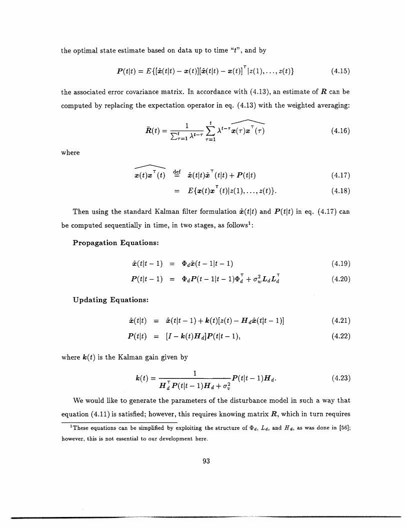
the optimal state estimate based on data up to time "t", and by
P(tlt) = E{[x(tlt)- _ (t)][(tlt)- X(t)] Iz(1),...,z(t)} (4.15)
the associated error covariance matrix. In accordance with (4.13), an estimate of R can be
computed by replacing the expectation operator in eq. (4.13) with the weighted averaging:
t
R(t) = t A- A - r x(r)xT (r) (4.16)~'~=1 'r=l
where
x(t)x r (t) adf :i(tjt);i (t~t ) + P(tlt) (4.17)
= E{X(t)x T (t)lz(1), .. , z(t)}. (4.18)
Then using the standard Kalman filter formulation :i(tIt) and P(tlt) in eq. (4.17) can
be computed sequentially in time, in two stages, as follows1 :
Propagation Equations:
k(tt- 1) = 1dk(t- lt- 1) (4.19)
P(tt - 1) = 'dP(t- lt- 1))' + ,2 LdL' (4.20)
Updating Equations:
i(tjt) = i(tlt- 1) + k(t)[z(t)- Hdi(tIt- 1)] (4.21)
P(t t) = [I - k(t)Hd]P(tlt- 1), (4.22)
where k(t) is the Kalman gain given by
k(t) = 1 P(tIt - 1)Hd. (4.23)Hd P(tIt - 1)Hd + UV
We would like to generate the parameters of the disturbance model in such a way that
equation (4.11) is satisfied; however, this requires knowing matrix R, which in turn requires
1These equations can be simplified by exploiting the structure of d, Ld, and Hd, as was done in [56];
however, this is not essential to our development here.
93
knowing the exact parameters of the disturbance model. Instead, we propose generating
these parameter estimates in such a way that the following equation is satisfied:
l) ,~ l ~(4.24)')
where R(t) is the estimate of R, obtained by performing the weighted averaging:
t1R(t) = t t - T Atx(r)X () (4.25)
ET= I r=1
where
x(t)x (t) def (tjt)i (tjt) + P(tt), (4.26)
where 5i(tlt) and P(tlt) are the estimate of the state and its covariance, computed using
the Kalman filtering equations (4.19)-(4.23), where instead of ca and a2 we use the most
current estimates &(t) and 2(t), i.e.
Propagation Equations:
5i(tlt- 1) = 4 d(t)(t- lit- 1) (4.27)
P(tjt - 1) = ~d(t)P(t- 1it- 1)~T(t) + o2 (t)LdLT (4.28)
Updating Equations:
T(tjt) = i(tt - 1) + k(t)[z(t)- Hd (tt- 1)] (4.29)
P(tlt) = [I- k(t)Hj]P(tit- 1), (4.30)
where id(t) is the matrix defined in eq. (4.8) computed at a = &(t), and k(t) is the vector
defined in eq. (4.23) with P(tlt - 1) obtained from eq. (4.28).
Our goal now is to develop a sequential procedure for generating the parameter estimates
in accordance with equation (4.24), i.e. the parameter estimates at time t + 1, &(t + 1) and
a'2 (t + 1), must satisfy equation (4.24). To obtain this sequential procedure for updating
the parameter estimates, we define
Q1 1 (t) Q 1 2 (t) t= Q (t) = A'-' X(r)X (7 ) (4.31)
Q21() Q(t) r=1
1 P
94
1R(t)
6,(t + 1) i

= x(t)x T (t) + AQ(t - 1). (4.32)
Using eq. (4.31) and eq. (4.25), we express eq. (4.24) as I =[+)] (4.33)
which leads to the following update equations for the noise parameter estimates:
&(t + 1) = -Q2-1(t)Q 21 (t) (4.34)_-- 1-A
2 (t + 1) 1 - At[Q11(t) + Q 12(t)a(t + 1)], (4.35)
where we have used the fact that Ft, _ 1_- .We shall refer to eqs. (4.34)- (4.35) as
the non-gradient algorithm.
At each time step the non-gradient algorithm first estimates the current state using
the latest parameter estimates in eqs. (4.27) - (4.30), and then updates the parameter
estimates using the state estimate just computed and its covariance in eqs. (4.34)- (4.35).
The intermediate quantity Q(t) is computed recursively in time according to eq. (4.32).
The factor A that appears in the cumulative averaging in eq. (4.31) is a number between
0 and 1. To maximize statistical stability we choose A = 1. Choosing A to be strictly smaller
than 1 corresponds to exponential weighting that gives more weight to current data samples
and results in an adaptive algorithm that is capable of tracking non-stationary changes in
the structure of the data.
As an alternative to the parameter update equations (4.31)- (4.35), we may consider a
gradient-search algorithm for solving the Yule-Walker equation (4.11). In this case, instead
of the signal correlation matrix R we use its estimate given by eq. (4.25), and we proceed
sequentially through the data using a stochastic gradient type procedure [43]. Replacing R
in eq. (4.11) by its current estimate R(t) = ll_ Q(t) where Q(t) is defined in eq. (4.31),
we obtain:
Q21(t) + Q 22(t)a = o (4.36)
2 1-Aw - I N[Q 11(t) + Q12(t)a] = 0. (4.37)
95
I Q11(t) -Q 12 (t)
t - rET=1 At Q21(t) Q22(t)
L J

From eqs. (4.36) and (4.37) and using an approach similar to that used in compound decision
problems (e.g., see [25, 38, 42, 45, 54]), the following sequential update equations for the
signal parameters are suggested:
&(t + 1) = &(t) - t[Q21(t) + Q 22(t)&(t)] (4.38)
c2 (t + 1) = o2 (t) - yt [(t) - t [Q ( t ) + Q22(t)(t)] (439)
where Qij(t) i,j = 1,2 are computed recursively in t using eq. (4.32), and yt is the step-sizes
of the stochastic gradient algorithm. We shall refer to eqs. (4.38)-(4.39) as the gradient
algorithm.
The advantage of using the gradient algorithm specified by eq. (4.38) - (4.39) is that
it does not require matrix inversion in contrast to the non-gradient algorithm specified by
eqs. (4.34)-(4.35), and therefore the gradient algorithm is computationally simpler than the
non-gradient algorithm.
4.4 Algorithm Performance
The results of applying the algorithms developed in the previous section to synthetically
generated noise and to recorded aircraft noise are presented in this section.
4.4.1 Synthetic Noise
Two sets of experiments were performed in which the gradient algorithm of the previous
section was applied to computer generated autoregressive time series. The first set of
experiments was performed to show how close the estimated spectrum of the AR process
matches the actual spectrum. The second set of experiments was performed to calculate
the one-step-ahead prediction error that results from using the estimated parameters. This
prediction error was then compared to the one-step-ahead prediction error that results from
using the correct parameters. In all these experiments the model order and a, were assumed
to be known exactly. The variance of the AR process (E{n2(t)} in (4.3)) was equal to 1 in
these experiments, and the forgetting factor A was set equal to 0.975.
96
The first set of experiments presented in this section illustrates how accurately the
algorithms developed in this chapter can estimate the model for the unwanted noise that is
needed to compute the optimal controller of Chapter 3. The design procedure of Chapter
3 relies solely on the second-order statistics of the unwanted noise and the measurement
noise. Since the measurement noise is assumed to be white, we can equivalently say that
the design procedure of Chapter 3 relies solely on the power spectrum of the unwanted noise
and the variance of the measurement noise. Therefore, it is important to see how close the
estimated power spectrum of the unwanted noise matches the actual power spectrum of the
unwanted noise.
In Fig. 4.2(a) and Fig. 4.3(a), the doted curve is the spectrum of the actual underlying
AR process, and the solid curve is the average estimated spectrum obtained by using the
gradient algorithm. The solid curve is computed by averaging the estimated spectrum over
6000 consecutive points. The actual system parameters for these two figures are:
1Fig.1: A(z) = l_1.53zl+.6z2 O = 0.234 aC = 0.05
(4.40)1
Fig.2 A(z) = l-1.8896zl+O.9O25z 2 Ow = 0.0501 o = 0.05.
In other words, the AR process was generated as the output of A(z) with a white noise
input of variance o2input f varance w .
In Fig. 4.2(b) and Fig. 4.3(b), the dotted horizontal line is the average one-step-ahead
prediction error of a Kalman predictor that uses the correct system parameters. This is
the optimum predictor, in the sense that no other predictor can achieve a lower average
prediction error. The solid curve in these two figures is the average prediction error obtained
by using the gradient algorithm.
4.4.2 Aircraft Noise
The results of applying both the gradient and the non-gradient algorithm to three types of
aircraft noise are presented in this section. These two algorithms were used on the noise
generated by a propeller aircraft, a helicopter, and a jet aircraft. Recordings of these three
types of noise were made from a microphone placed inside a set of headphones approximately
97

two meters away from each aircraft. Note that these recordings correspond to z(t) in eq.
(4.3).
These experiments simulate an indirect adaptive feedback controller in which the plant
is a known delay of M samples, i.e. G(z) = z - M. In Fig. 4.1, with G = z - M, the feedback
controller that minimizes E{(n(t) + c(t))2 } is the M-step-ahead predictor that generates the
LLSE of -n(t) based on {m(r) r < t - M}, i.e. the optimal canceling signal c(t) in this
case is the LLSE of -n(t) based on {m(r) r < t- M}. The resulting residual signal e(t)
in this case is the corresponding M-step ahead prediction error, i.e.
e(t) = n(t) - E{n(t)lm(T) r < t - M}. (4.41)
The performance of the adaptive feedback controller in this case depends on how well n(t)
can be predicted based on {m(r) r < t- M}, or equivalently based on {z(r) r < t- M}.
In short the residual signal in this case is simply the prediction error in predicting n(t)
based on {z(r) r < t - M} and based on the estimated parameters of the noise model.
Several simulations were performed to illustrate how well n(t) can be predicted based
on measurements of {z(r) r < t - M} and based on the estimated parameters of the
model of the noise obtained from our gradient algorithm. In these simulations, the order
of the AR model for the unwanted noise was assumed to be five, and av was fixed at 5%
of the standard deviation of z(t). The algorithms were tried with the order of the AR
model ranging from three to nine, and it was found that the performance of the algorithm
improves very little by increasing the order beyond five. The variance of the microphone
measurement noise, ao, can be estimated in the following way. The microphone is placed
in a quiet environment with the ANC turned off so that the output of the microphone is
approximately v(t). An estimate of a2 can then be obtained as
N
C' t v2(t) (4.42)t=l
Figure 4.4 is a plot of the normalized prediction error versus the prediction time for the
non-gradient algorithm. Similarly, Figure 4.5 is the plot of the normalized prediction error
versus the prediction time for the gradient algorithm. In these two figures, the normalized
98
prediction error is calculated as
E{e2(t)}Normalized Prediction Error(dB) = 101og 10 E{z2 (t)}' (4.43)
where E{z2 (t)} is the average power of the original recorded noise, and E{e2(t)} is the
average power of the prediction error.
An intuitive explanation for why the normalized prediction error of the propeller noise
is less than the normalized prediction error of the helicopter noise and the normalized
prediction error of the jet noise. The propeller noise is more narrow-band than the helicopter
noise and the jet noise; therefore, the propeller noise results in the least prediction error.
Furthermore, it is evident from these set of experiments that the performance of the
gradient algorithm is slightly better than the non-gradient algorithm. Furthermore, the
gradient algorithm is much less computationally intensive than the non-gradient algorithm.
4.5 Summary
Two recursive/adaptive algorithms for modeling the unwanted noise at a single microphone
were presented in this chapter. We argued that if the plant model is exactly known, these
algorithms can be combined with the design procedure of Chapter 3 to obtain an adaptive
feedback ANC system. Of course, it is eventually necessary to fully develop these algorithms
so that the disturbance model and the plant model are both adaptively estimated.
We assumed that the unwanted noise was a non-stationary autoregressive process, and
that the observed signal was the sum of this autoregressive process plus white measurement
noise. We then developed two algorithms for estimating the parameters of this autoregres-
sive process based on the observed data. The performance of these algorithms were studied
by applying them to synthetically generated noise and recorded aircraft noise. It is worth
noting that these algorithms can be applied to the more general problem of identifying
non-stationary autoregressive processes embedded in white noise.
99

Ideal and Estimated Spectrum
m
a).'.-aC"
0 0.5 1 1.5 2 2.5 3 3.5
Frequency(Radians)(a)
Ideal and Realized Prediction Error11.t
(.5
r"04' 0.4
5a)a(9)
03
C 0.2CZ.
C)(.1
0 10 20 30 40 50 60
Time(xl 00)
(b)
Figure 4.2: Performance of the gradient algorithm on synthetic noise.
100
TI
III1*4.
I, II t_"} -L J I
i i i I I I I II I I I I
.... T...-.-----'
--- I .. �1 - - - - L - - - I - - - - -.
I I I I II I I I II I I I I
I I I I II I I I II I I I II

Ideal and Estimated Spectrum
Frequency (Radians)
(a)Ideal and Realized Prediction Error
C0
4)~
0
-oC
CU
10 20 30 40 50 60
Time(x100)
( b )(b)Figure 4.3: Performance of the gradient algorithm on synthetic noise.
Figure 4.3: Performance of the gradient algorithm on synthetic noise.
101
rn4)-c
C
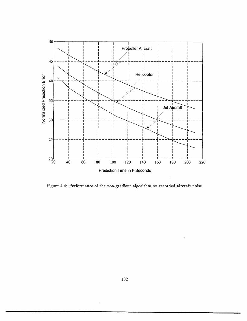
,u
45
III0wC.o0
U,ra
Va_a)N
E0z
40 60 80 100 120 140 160 180 200 220
Prediction Time in [t Seconds
Figure 4.4: Performance of the non-gradient algorithm on recorded aircraft noise.
102
i l l l l l II I I I I I I I II I I I I I I I IIIII I I I I
"Iwi i i i i i i i
To
or eJ&
20
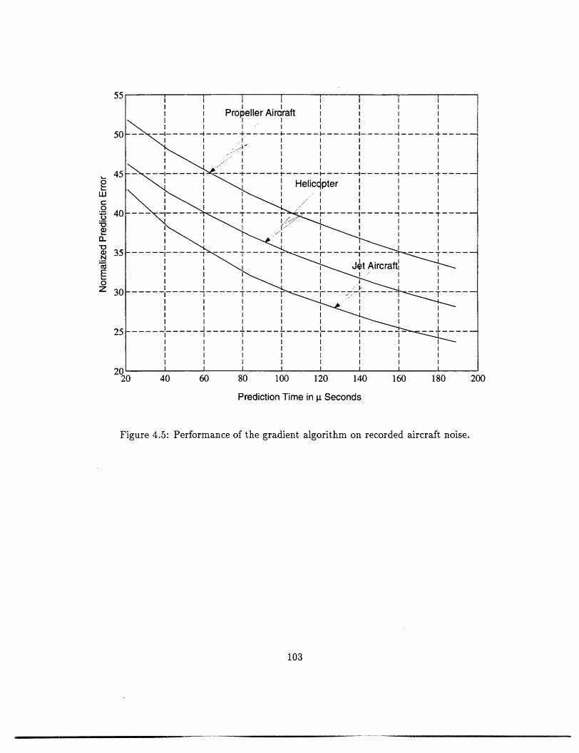
o
LIJC0.o
V._o-
a)N
E0z
Prediction Time in !x Seconds
Figure 4.5: Performance of the gradient algorithm on recorded aircraft noise.
103
-------- -
10

Chapter 5
Distributed Optimal Feedback
Control for ANC
5.1 Introduction
Our treatment of the active noise cancellation (ANC) problem up to this point has been
limited to pointwise active noise cancellation. In Chapter 3, we developed an optimal
feedback controller for attenuating the acoustic pressure at the locations of a finite number of
error microphones. Specifically, this controller minimizes a performance criterion involving
the average power of the residual pressure field at the location of the error microphones
and the average power of the control signal. Hence, this pointwise criterion depends only
on the interaction between the primary field and the canceling field at those points where
the microphones are located.
The distributed active.noise cancellation problem is studied in this chapter. Specifically,
we develop an optimal feedback controller for minimizing a performance criterion involving
the total acoustic energy in an enclosure and the power expended by the control signal. To
minimize this distributed performance criterion, the interaction between the primary field
and the canceling field at every point in the enclosure needs to be considered.
Our approach is to formulate the distributed ANC problem as an infinite dimensional
feedback control problem and use existing control theory to solve it. The deterministic for-
104

mulation, which assumes that the entire state is observable, and the stochastic formulation,
which estimates the state based on the available observations, are both considered. The
main assumption is that the boundary surrounding the volume of interest is either purely
reflecting or purely absorbing.
Our formulation of the distributed ANC problem in this chapter is remarkably similar
to our formulation of the pointwise ANC problem in Chapter 3. In Chapter 3, the unwanted
noise signal was modeled as the output of a linear system driven by white noise, and the
canceling signal was modeled as the output of another linear system driven by the control
signal. In this chapter, the unwanted noise field is modeled as the output of a linear system
driven by white noise, and the canceling field is modeled as the output of yet another linear
system driven by the control signal. In Chapter 3, the linear systems were finite dimensional
and were characterized by differential equations. In this chapter, the linear systems are
infinite dimensional and are characterized by partial differential equations. The optimal
control in either case is a linear feedback of the state estimates. Furthermore, in both cases,
the state estimates are computed using a Kalman filter, and the feedback gain is obtained
from a Riccati equation.
Section 5.2 is essentially background material and terminology that is needed to under-
stand our formulation of the distributed active noise cancellation problem in the determin-
istic case. The deterministic quadratic regulator problem is presented in Section 5.3. The
acoustic system that we focus on and its governing equations are presented in Section 5.4.
In Section 5.5, we derive an abstract differential equation representation for this acoustic
system and show that the noise cancellation problem for this system is equivalent to a
deterministic quadratic regulator problem.
The stochastic formulation of the distributed active noise cancellation problem is pre-
sented in Section 5.6. The necessary measure theoretic structure is introduced in Section
5.6.1, followed by the stochastic quadratic regulator problem in Section 5.6.2. In Sec-
tion 5.6.3, the noise cancellation system that we focus on is modeled as a linear infinite-
dimensional system driven by a white noise process and a control process. Furthermore,
we show that this model can accommodate an observation process that is the output of a
105

pressure microphone, and a control process that is the input to an ordinary loudspeaker.
Finally, we show that the distributed active noise cancellation problem for the acoustic
system that we focus on is equivalent to a stochastic quadratic regulator problem.
5.2 Preliminaries
This Section contains the terminology and background from functional analysis that is
needed to understand our particular formulation of infinite-dimensional linear systems.
General properties of semigroups are presented in Section 5.2.1, and abstract differential
equations are presented in Section 5.2.2. Proofs for almost all the theorems in this Section
can be found in [5].
5.2.1 General Properties of Semigroups
Let T(t), t > 0 be a family of linear bounded transformations mapping a Hilbert space H
into itself. T(t) is said to be a "semigroup" if
(i) T(O) = Identity
(ii) T(tl + t 2) = T(t 2 )T(tl)= T(tl)T(t2).
The semigroup T(t) is said to be strongly continuous if for each x in the Hilbert space H
(iii) IT(t)x-xI I-)0 as t )0 + .
Using (i)-(iii), one can show that T(t) is bounded on bounded domains; that is, for each
L < o, there exists an M such that
Sup IIT(t)II M < oo.0 < t < L
Moreover, we can find a dense subspace of H on which T(t) is differentiable. That is, we
can define the operator A (called the infinitesimal generator of T(t)) as
Ax = lim T(A)x - xA(o+ A
D(A) = {x E HI lim ( exists}A_+ A
106

where D(A) is the domain of A. Note that operator A is a mapping from D(A) into H.
From the above definition of A it follows that T(t)x is differentiable on DA for all t > 0
and
d(T(t)x) = T(t)Ax = A(T(t)x) x E D(A).
This definition of A also implies that A is a closed linear operator and its domain is dense
in H.
The relationship between the semigroup T(t) and its infinitesimal generator A is similar
to the relationship between the matrix exponential eA t and the matrix A where
+eAtx = AeAtx.dt
It will be seen later that this analogy can be carried much further. For example, eAtx(O) is a
solution to the system of ordinary differential equations d x(t) = Ax(t). Similarly, T(t)x(O)
is a solution to the abstract differential equation d x(t) = Ax(t), provided that A is the
infinitesimal generator of the strongly continuous semigroup T(t).
We now state two theorems regarding the necessary and sufficient conditions for a dissi-
pative linear operator to be the infinitesimal generator of the strongly continuous semigroup
T(t). Recall that a closed linear operator A mapping a Hilbert space H into itself and with
dense domain D(A) in H is said to be dissipative if
[Ax, x] + [x, Ax] < 0 Vx E D(A). (5.1)
We already have seen that the infinitesimal generator of a strongly continuous semigroup
must necessarily be closed with dense domain in H. A closed linear operator that maps a
Hilbert space into itself and has a dense domain will have a unique adjoint operator whose
domain is also dense [33].
Theorem 1 Let A be a closed linear operator with dense domain in a Hilbert space
H, and assume that A maps its domain into H. Suppose further that both A and A*, the
adjoint of A, are dissipative. Then A generates a strongly continuous semigroup T(t) such
that liT(t)jI < 1 for all t > 0.
107

Theorem 2 Suppose A is a closed linear operator with dense domain D(A) in a Hilbert
space H. Suppose further that A maps its domain into H, and
= [Ax, ] + [, Ax] V E D(A)
0 = [A*x, x] + [, A*x] Vx D(A*),
where [.,.] is the inner product in H. Then, A generates a strongly continuous semigroup
T(t) such that IIT(t)xll = llxll Vx E H.
From the last two theorems, we see that the semigroup generated by a dissipative linear
operator, call it T(t), is a contraction, i.e.
IIT(t)xl < llxll Vx E H.
A contraction semigroup will obviously have the property that IIT(t 2)xjj < IIT(tl)xll for all
tl < t 2. This property is analogous to the following property for a matrix A: if [Ax, x] +
[x, Ax] < 0 for all vectors x, then lileAt2xIl < lieAt ' xIl for all t < t 2.
5.2.2 Abstract Differential Equations: Cauchy Problem
The initial value (Cauchy) problem for first order linear abstract differential equations is
introduced in this Section. With the aid of semigroup theory, these abstract differential
equations are put in a framework very similar to that of ordinary differential equations. A
specific example is given to illustrate how a partial differential equation can be viewed as
an abstract differential equation.
Let A be the infinitesimal generator of a strongly continuous semigroup T(t) in a Hilbert
space H. The initial value problem for the abstract differential equation:
dx(t) = Ax(t) x(0) is given and is inD)(A) (5.2)dt
is to find the function x(t) with range in Hilbert space H that satisfies (5.2). Then, x(t) =
T(t)x(O) gives one solution, since (T(t)x(0)) = A(T(t)x(O)) and T(0)x(0) = x(0). This is
the only solution under the additional assumptions that:
1. x(t) E D(A) t > O
108

2. x(t) is absolutely continuous for t > 0
3. Ix(t) - x(0)II 0 as t ) 0+.
From the above discussion, we see that in the case of abstract differential equations T(t)
plays a role analogous to the state transition matrix for ordinary differential equations.
Next we consider the nonhomogeneous equation
dx(t) = Ax(t) + u(t) 0 < t < T (5.3)
with a given initial condition x(0). By analogy with the finite dimensional case, we would
expect that
x(t) = T(t)x(O) + j T(t - s)u(s)ds
should be the unique solution in an appropriate sense. Depending on the smoothness of
u(t) and whether x(0) is in D(A) or not, the sense in which (5.3) is satisfied will vary. The
next two theorems are concerned with this issue.
Theorem 3 Suppose x(0) is in D(A), and the function u(t) with range in Hilbert
space H is strongly continuously differentiable in the open interval (0, T) with derivatives
continuous in the closed interval [0, T]. Then
dx(t) = Ax(t) + u(t) 0 < t < Tdt
has a unique solution satisfying
1. x(t) E D(A) t > 0
2. x(t) is absolutely continuous in (,T)
3. Ix(t)- x(0)II - 0 as t 0 + ,
and this solution is given by
x(t) = T(t)x(O) + j T(t - s)u(s)ds.
If we wish to consider the case where neither the condition that x(0) belongs to the
domain of A, nor the condition of smoothness on the input u(t) hold, we have to change
the sense in which equation (5.3) holds.
109
Theorem 4 Suppose u(.) E £ 2 ((0,T);H), then there is one and only one function
x(t), 0 < t < T, such that [x(t), y] is absolutely continuous for each y in D(A*), and
dd[x(t), y] = [x(t), A*y] + [u(t), y] a.e. 0 < t < T, (5.4)
and such that for a given x(0) in H,
lim [x(t), y] = [x(0), y] Vy E D(A*).t- O+
Moreover, this function is given by
= r~~~~~~tx(t) = T(t)x(O) + J T(t - s)u(s)ds.
The following example illustrates how a partial differential equation can be viewed as
an abstract differential equation in an appropriate function space.
Example: Application to Partial Differential Equations
Consider the partial differential equation for one-dimensional heat transfer
a f(t,x) = 9 2 f(t,x) t > 0 ;-oo < x < oo ;f(0, x) is given.
Let us show that this partial differential equation can be represented as an abstract differ-
ential equation of the type discussed in the previous Section. For this, we need to show
that a2 is an infinitesimal generator of a strongly continuous semigroup. Note that it is
not necessary to explicitly find the semigroup generated by a2; all that is needed to is to
show that such a semigroup exists.
First we choose the underlying Hilbert space to be H = £2(-00, °°), the space of square
integrable functions with respect to the Lebesgue measure. Next we take A = as our
linear operator with the following dense domain
D(A) = {f(z) E HIf, fare absolutely continuous and f',f" E H}.
This means in particular that f(-oo) = f(oo) = f'(oc) = f'(-oo) = 0. Domain of A is
dense in H, since the C ' , the set of all infinitely differentiable functions in L2(-oo, +oo),
is included in the domain of A, and C ° is dense in H as shown in [1].
110

Using integration by parts, we can show that operator A is self adjoint:
[g, Af] = Jg(x) aX2fdx= _ g o 9 fgdx
= [Ag,f]. Vf,g E D(A) (5.5)
Again using integration by parts, we see that A is dissipative since
[fAf] = fW- 2fdx = - ) ) dx < O.foo X E. TX '9o
It follows that operator A is closed, since it is self adjoint and A* is closed by the
virtue of being an adjoint operator [33]. A is a closed linear operator with dense domain
in H, and both A and A* are dissipative; therefore, by theorem 1, A generates a strongly
continuous contraction semigroup T(t). The original partial differential equation can now
be represented as an abstract differential equation:
d+f(t) = Af(t) t > 0; f(0) E D(A) is given, (5.6)
where
2A = _x
D(A) { f(x) e HIf,f'are absolutely continuous and f',f" E H}.
Note that f(t) = T(t)f(O), where T(t) is the semigroup generated by A, is a solution to
(5.6) since
d (T(t)f(O)) = A(T(t)f(O)),dt
and T(t)f(O) is in the domain of A for all values of t with T(O)f(0) =.f(0). In summary, we
have shown that the operator A = 82 is the infinitesimal generator of a strongly continuous
semigroup T(t), and hence been able to represent the original partial differential equation
as an abstract differential equation in the Hilbert space £2(-oO, +oo).
Having discussed abstract differential equations, we will present the control problem for
systems governed by these equations in the next Section.
111
- -

5.3 Deterministic Linear Quadratic Regulator Problem
The linear quadratic regulator problem for systems governed by abstract differential equa-
tions is presented in this Section. We will see that under very mild conditions, a unique
feedback solution to this problem exists.
Let A denote the infinitesimal generator of a strongly continuous semigroup of operators
T(t) over a Hilbert space H. The dynamic equation governing the problem is
dx(t) = Ax(t) + Bu(t) < t < T < oo (5.7)
x(0) given,
where B is a linear bounded transformation mapping a Hilbert space H, into H, and u(.)
is an element of Wu = £ 2 ((O, T); H,). It follows that Bu(.) is an element of £2((0, T); H).
Hence, a unique solution to (5.7), in the sense of (5.4), exists and is given by
rtx(t) = T(t)x(O) + j T(t - s)Bu(s)ds.
The optimal control problem is to find u(t) in WVu so that the cost functional
J = ][Rx(t), x(t)]Hdt + [u(t), U(t)]Hdt (5.8)o0 o
is minimized, where R is a linear bounded nonnegative definite operator mapping H into
H. The first integral in this functional is essentially what we want to minimize, and the
second integral is the amount of power expended by the control input u(t).
It is well known [5] that the above problem has a unique solution u(t) which can be
expressed in state feedback form as
uo(t) = -B*K(t)xo(t), (5.9)
where K(t), for each t, is a linear bounded transformation from H into H and is absolutely
continuous in t, 0 < t < T. Furthermore, K(t) satisfies the operator Riccati equation
d [IK (t)x,y] = -[Rx,y] - [K(t)x,Ay] - [K(t)Ax,y] (5.10)
+[K(t)BB*K(t)x,y]. K(t) = 0 Vx,y E D(A)
112

Hence, if we can formulate the distributed active noise cancellation problem as a linear
quadratic regulator problem, we will be able to use the above result to find the unique
solution to the distributed active noise cancellation problem. Furthermore if such a solution
exists, it will be expressible in feedback form.
The acoustic system that we focus on in this chapter and its governing equations are
presented in the next Section. Our ultimate goal is to represent these equations as abstract
differential equations of the type discussed in Section 5.2.2.
5.4 Dynamics of Two Deterministic Acoustic Systems
The governing equations of the acoustic systems that we focus on in this chapter are pre-
sented in this Section. The second order wave equation for pressure is broken up into two
first order partial differential equations, so that it can be later represented as an abstract
differential equation in Section 5.5.
Sound essentially involves a weak motion of a non-viscous fluid from an initial state of
rest [16]. Particle velocity v(t, x) and pressure p(t, x) are the two physical quantities whose
values completely characterize any acoustic system, where the underline denotes a vector-
valued quantity; t is the continuous-time variable; and x is the spatial variable. These two
quantities are related according to the following partial differential equations:
V p(t,x) = Po o(t) + f(t,X) (5.11)
1 ap(t,x)V. (t, ) = -c 2p ot)' (5.12)
where f (t, x) is an external force field; P0 is the ambient density; c is the speed of sound;
V. v is the divergence of v; and VP is the gradient of P. The first equation is obtained by
applying Newton's law to a small control volume, and the second equation is obtained by
applying the conservation of mass principle to this volume. The familiar wave equation for
p(t, x) can be derived from the above equations by differentiating eq. (5.12) with respect
to time, taking the divergence of eq. (5.11), and eliminating V.( a t )) to get:at
1 o&2 p(t, x) _ 2p(t,x) - V. (f_(t,x (5.13)c2 at2
113

, where V2 is the three dimensional Laplacian. Equations (5.11) and (5.12) are two
first order partial differential equations equivalent to the second order partial differential
equation (5.13). For us, it is more convenient to work with the following arrangement of
(5.11)-(5.12):
a f P9l =[0 PcV. PO + Bu(t), (5.14)c v(tx) -cV 0 c v(t, x)
where B is a bounded linear operator relating the control input u(t) to the force field f(t, x)
so that
0Bu(t) =
P0f(t,X)
I;
Figure 5.1: Enclosed region in R 3 with boundary r.
Next let us specialize the above equations to an enclosed region in R 3. We shall do
this specialization for two types of boundary conditions. The first kind of boundary to
be considered is a perfectly reflecting one, i.e. the normal component of velocity at the
boundary surface is assumed to be zero. The second kind of boundary to be considered
is an absorbing one, i.e. the ratio of the pressure at the boundary surface to the normal
component of particle velocity at the boundary surface is assumed to be a known positive
114

real number. This ratio is called the acoustic impedance of the the boundary; hence, in
the second case we are assuming that the impedance of the boundary is purely resistive.
The most general type of boundary condition is obtained when this ratio, in the frequency
domain, is a complex valued function H(w), where w is the frequency variable. The most
general case is not considered in this chapter.
5.4.1 Purely Reflecting Boundaries
In Fig. 5.1, let Q be a bounded open domain in R 3 with smooth boundary r. Furthermore,
assume that eq. (5.14) is satisfied for all the interior points of Q with
v'(tX) = x E , (5.15)
where vn is the normal component of velocity at the boundary. Finally, assume that the
following initial conditions are given:
P(O,x) = Po(x) and v(O,)= VO(x).
The total acoustic energy of the system in Fig. 5.1 at time t, denoted by E(t), is
E(t) = J P2(t x)dx + P±I4V(tX 2dx,o2c2 PO 0
where the first integral is the total acoustic potential energy and the second integral is the
total kinetic energy.
With the boundary condition eq. (5.15) and with no input u(t), it can be easily shown
[16] that E(t) is constant as a function of t. This is consistent with our assumption that
the boundary surfaces are lossless and that there is no input to the system; hence, there is
no mechanism to increase or decrease the acoustic energy in this case.
5.4.2 Purely Absorbing Boundaries
Again in Fig. 5.1, let Q be a bounded domain in R 3 with smooth boundary F. Furthermore,
assume that eq. (5.14) is satisfied for all the interior points of Q with the following boundary
condition
p(t,X) = +Z(X) v (tX) E r, (5.16)
115
- | a -

where vn is the normal component of the velocity field at the boundary, and Z(x) is a
positive real number. Again, we assume that the following initial conditions are given:
P(O, x) = P(x) and v(0, x)= 0(x).
The purpose of active noise cancellation is to choose the signal u(t) in such a way that
the resulting force field f (t, x) does negative work on the system and thereby reduces the
acoustic energy of the system. Naturally, one would like to decrease E(t) without expending
too much power; hence, a reasonable performance criterion for an active noise cancellation
system is the sum of the acoustic energy E(t) and the power expended by the control
input u(t). We would like to formulate the active noise cancellation problem as an abstract
quadratic regulator problem with the cost function equal to this sum. To this end, we first
need to derive an abstract differential equation representation for the acoustic system of
Figure 5.1.
5.5 Abstract Representation of Two Deterministic Acous-
tic Systems
The goal of this Section is to derive an abstract differential equation representation for the
acoustic systems of Fig. 5.1 subject to the boundary condition specified by eq. (5.15) or
specified by eq. (5.16). This derivation is achieved by showing that the differential operator
0 -c V.A = (5.17)
-cV 0
is an infinitesimal generator of an absolutely continuous semigroup in an appropriate Hilbert
space. Once this abstract representation is established, it will be easy to show that the
noise cancellation problem in Fig. 5.1 is equivalent to a quadratic regulator problem. The
existence and uniqueness of the solution to the noise cancellation problem will then follow
from the existence and uniqueness theorems for the solutions of the abstract quadratic
regulator problem.
116

The first step toward establishing the abstract formulation is to choose the underlying
Hilbert space and the domain of A in this space. For this, let us define
Hl(Q) = f E 2() exists and f e £ 2(FQ) fori = 1,2,3},
where £ 2(Q) is the class of square integrable functions with respect to the Lebesgue measure
that are defined on Q, and we further define
M = (F) x H'(QF) x H'(Q) x Hi(Q). (5.18)
The underlying Hilbert space H is
H = £2 (Q) x L2(Q) x L2() x 2(Q), (5.19)
with the following inner product
4
[e,h]H = Z[ei,hi] 2 (Q) Ve,h E H.i=e
5.5.1 Purely Reflecting Boundaries
In the case of purely reflecting boundaries, the linear operator A is defined as:
A P -c V. (v) 1 [P|A V E/D(A)
v -c V(p) v}
'D (A) = | P E M 0--~ = 0; V¥x e r ,v
(5.20)
(5.21)
where v(Lx) is the normal component of the velocity field at the boundary. Using the
divergence theorem in R3, we can show that A* equals the negative of A:
,A I], = [v|1 e )(A)
L2 L2 ., LL2 J -¢ V J2(f ) f2
=-C g1(x)V. (L 2(x))dx - Hf [g2,V ()]R3dx (5.22)
117

= cf L[f2 V (g9l)]R3dx - cjr a ( 2f)ds +
c f fV. (g 2)dx (5.23)
C V(gil) f 2j
cf a (g2fi)ds, (5.24)
where in transition from eq. (5.22) to eq. (5.23) we have used the divergence theorem in R 3
and the fact that on the boundary -- = 0. This is essentially a three dimensional version
of the integration by parts that was done to get eq. (5.5) in Section 5.2.2. The domain
of operator A defined in eq. (5.21) is dense in H, since CO(F), the set of all infinitely
differentiable function with compact support in Q, is dense in £2(Q) as shown in [1].
We see that the surface integral in equation (5.24) must equal zero; hence, A* is
A* 1 l = () -A 1 V (12) =-AL D(A*)
Lg2J L CV(gi) Lg2 Lg2
D(A*) =
Closedness of the operator A
tors are closed [33]. Next, using
f[4]7 fll
91MI O2 ()On =0 VXe r.
R2 j Jfollows immediately since A* = -A and all adjoint opera-
the divergence theorem, we show that A is dissipative:
-[ V(fl) 1 L2 ||H
- cJ v (fL2 )fidx - c [V(f),f 2]R3dx (5.25)
f[f 2 , V(flijR3dx - C [V(fh), L 2]R3dx (5.26)
= 0, (5.27)
where in transition from eq. (5.25) to eq. (5.26), we have used the divergence theorem and
the fact that on the boundary = O.
118

Combining eq. (5.27) with A* = -A, we get
= [Af,f]+ [f,Af] Vf e D(A) (5.28)
= [A*g,g] + [g, A*g] = 0 Vg E D(A*). (5.29)
We have therefore shown that A is a closed, linear and dissipative operator with dense
domain in H. Moreover, A satisfies (5.28) and (5.29). Applying Theorem 2, it follows that
A generates a strongly continuous semigroup T(t) on H such that
IIT(t)f IH = fI IH Vf e H.
From the last expression we see that T(t) is norm preserving. This can be interpreted as
saying that the acoustic energy of the system in Fig. 5.1 with the boundary condition
specified by eq. (5.15) is constant, since the norm in H is proportional to the acoustic
energy in the enclosure.
5.5.2 Purely Absorbing Boundaries
In the case of purely absorbing boundaries, the linear operator A is defined as:
A = [ (v) V [(A) (5.30)
v cL CV(P) I LvJ
D(A) = e MI p(x) = Z(x) Ov() Vx e r. (531)
Using the divergence theorem in R3 , we find A* and its domain:
,1 A , 1 C1.2)v E VD(A)gl ]f ,i ] = l ]- cV..f ] [ fl ] DA
K 92 f 2 H2 -c V(fl) H f2
= cJ gl(x)V. ( 2(x))dx - cJ [ 2,V (fl)]R3dx (5.32)
c J[L2, V (gl)]R3dx - cf a(f 2gl)ds +
119
--

CJ f1 V. ( 2)dx - j a(g 2fi)ds (5.33)
c V(g) f 2 JJ
-c{j Q-(f2 g1 )ds + r -(g 2fi)ds}, (5.34)
where in transition from eq. (5.32) to eq. (5.33) we have used the divergence theorem in
R 3. The domain of operator A defined in eq. (5.31) is dense in H, since CO((Q) is included
in the domain of A, and CO is dense in H as shown in [1].
From eq. (5.34), we see that the expression in the brackets must equal zero. By equating
this expression to zero and recalling eq. (5.16), we get the following expression for A*:
91 F CV. (_2 ) 1 = -1
1 [1lA* = j=-A V EE(A ; )
L2 LC V(g1 ) L92] L£2J
[1 0i9 E I g(~=-( g2 (X)D(A*) = M 91(x) = Z(x) -2(-) Vx r.
Ong2 J
Using the above derivation for A*, we see that operator A is the adjoint of the linear
operator B defined as
B[ = [ () ] E e )(B) (5.35)
g LcV( ) g LgJ
D(B) = E [ M f(x) = -Z(x) j_(_) V-x E I'. (5.36)
LgJOperator A must then be closed, since the adjoint of B is closed. Recall that all adjoint
operators are closed [33].
Next using the divergence theorem, we show that A is dissipative:
[A 1 II~ = K 2Ii-C V -2) iL L L 2 JJ H LL -CV(fl) J L f2 J
120

= cj V.(f 2)fidX - cj[V(f)f 2]R3dx (5.37)
= cf [ 2 ,V(fl)]R 3 dx - Cj -(f 2 f)ds
-C Jn[V(fi), L 2]R3dx (5.38)
= -cjZ(X) a ( 2fi)ds
= CZ(-) (a L 2 )2ds
< 0,
where in transition from eq. (5.37) to eq. (5.38) we have used the divergence theorem.
To get the last expression, we have used the assumption that on the boundary f(x) =
Z(X ) f2 (X) -
The operator A* is also dissipative, and this can be shown following steps very similar
to the one used to show that A is dissipative.
We have shown that A is a closed, linear and dissipative operator with dense domain
in H. Moreover, A* has also been shown to be dissipative. Applying Theorem 1, it follows
that A generates a strongly continuous semigroup T(t) on H such that
IJT(t)fIH < _|f[H Vf E H.
The last expression can be interpreted as saying that the mechanical energy of the system in
Fig. 5.1 with the boundary condition specified by eq. (5.16) is decreasing. This is consistent
with the fact that the boundaries in this case are assumed to be absorbing.
We have shown that the governing equation for the acoustic system of Fig. 5.1, with
purely reflecting boundaries or purely absorbing boundaries, can be represented as an ab-
stract differential equation of the form dtx(t) = Ax(t) + Bu(t), where A is the infinitesimal
generator of a strongly continuous semigroup.
We now write down the abstract differential equation representation for the system
in Fig. 5.1, subject to the boundary condition specified by eq. (5.15) or by eq. (5.16).
Assuming that u(.) is an element of Wu,, = £2((O, T); H,) and recalling that B is a bounded
linear operator from the Hilbert space H, into H, we arrive at the following abstract
121
--
- -

representation of the acoustic system in Fig. 5.1:
dx(t) = Ax(t) + Bu(t) (5.39)
x(0) is given in H,
where H is the underlying Hilbert space. Moreover, the operator A is defined by eq. (5.17),
and its domain is defined by eq. (5.21) in the case of purely reflecting boundaries and by
eq. (5.31) in the case of purely absorbing boundaries.
The distributed active noise cancellation problem can now be viewed as a linear quadratic
regulator problem applied to the system governed by eq. (5.39). Specifically, the objective
is to choose the input u(t) such that the the cost functional
rT rTJ= J E(t)dt + [u(t), u(t)]Hudt (5.40)
= A[22x(t), x(t)]Hdt + A[u(t), u(t)]Hdt (5.41)Jo 2c2
is minimized, where E(t) is the mechanical energy of the system at time t, and [u(t), u(t)]
is the power expended by the control input at time t. From eq. (5.9), we see that a unique
minimizing control u(t) in W~ exists and can be expressed in the state feedback form as
uo(t) = -B*K(t)xo(t),
where the linear bounded operator K(t) satisfies the operator Riccati equation
d .P0d[K(t)x,y] = -[2x,y]-[K(t)x,Ay] - [K(t)Ax,y]
+[K(t)BB*IK(t)x,y]. K(t) = 0 V, y E D(A) (5.42)
In summary, by formulating the distributed active noise cancellation problem as a lin-
ear quadratic regulator problem, we have been able to show that the distributed active
noise cancellation problem has a unique solution. Furthermore, we have given an explicit
expression for this solution as a linear feedback of the state of the system.
The main shortcoming of the above solution is that the control signal is generated based
on the exact knowledge of the entire state of the system. In a practical system, the state
is not known exactly and the control signal must be generated based on the observed data
122

alone (typically the observed data is the output of one or more microphones that are placed
in the volume of interest). It turns out that the optimal control in this case is obtained
by feeding back the estimate of the state. The resulting estimation and control problem
for infinite-dimensional linear systems is considered in the next Section. We will show that
the distributed active noise cancellation problem in which the control signal is based on
the observed data alone can be viewed as a stochastic quadratic regulator problem. The
noise cancellation problem can then be solved using the stochastic optimal control theory
for distributed parameter systems.
5.6 Stochastic Optimal Control for ANC
In this Section, the stochastic analog of the linear quadratic control problem of Section 5.3
is presented. For this purpose a measure theoretic structure is introduced on the top of the
topological structure. The measure theory is nonclassical in the sense that the measures
are only finitely additive on the field of cylinder sets. The notion of a weak random variable
suffices for the stochastic extension of the control problem of Section 5.3 with a crucial
notion being that of "white noise". The development of the stochastic control problem
presented here is entirely due to Balakrishnan [5].
5.6.1 Preliminaries
The measure theoretic background that is needed to understand our formulation of the
stochastic quadratic regulator problem is presented in this Section. Measures on cylinder
sets, weak random variable, "white noise" processes, and linear infinite-dimensional systems
with white noise input are discussed.
Measure on Cylinder Sets
Cylinder sets and cylinder set measures are introduced in this Section. We start with I a
separable real Hilbert space. Let us take any finite dimensional subspace Em in 7i. By a
123

cylinder set we mean any set of the form
where B is a Borel subset of 7 - m, and 7- is the orthogonal complement of 7'm. The Borel
set B is then called the "base" of the cylinder, and 7Hm is called the "base" space. It can
be shown that the class of cylinder sets C forms a field of sets. Furthermore, 7- itself is a
cylinder set, and the Borel sets of 7- are the smallest a-algebra that contains C.
Next we consider measures on the field of cylinder sets, these measures will be referred
to as "cylinder set measures" and denoted by y. Let Z be a cylinder set with base B in
Rm. Then by definition
Lt(Z) = vm(B),
where vm(.) is a countably additive probability measure on the a-algebra of Borel subsets
of 'rm. Furthermore Vm must satisfy the following condition.
Compatibility Condition: In order that u be well defined, it is necessary that if
Z = B + tc (B + p) + (m + .p)C,
where 7-p is orthogonal to T'm, then Vm(B) = Vm+p(B + Hp) where vm+p(.) is a countably
additive probability measure on the Borel subsets 7Hm + Hp.
It is important to realize that a cylinder set measure is not necessarily countably additive
on the field of cylinder sets. Consequently, a cylinder set measure can not in general be
extended to the Borel sets of 7-X.
The following example of a cylinder set measure will be of prime importance in our
development. Let R be any self adjoint nonnegative definite operator mapping X- into 7-H .
We define the measure on the Borel sets of any finite dimensional space Jim in the following
way. Let el,..., em be an orthonormal basis in 7-m. The Borel sets in 7m are in one-to-one
correspondence with the Borel sets in R m via the transformation
[x, el]
Xem]
Ix,era]
124
[X, el]
where x E 7Em and E R m . The measure on Borel sets of R m is defined to be a
[xem]
Gaussian measure with a moment matrix given by
rij = [Rei, ej] i,j = 1,.. .,m.
The measure of any Borel set in E-m is now defined to be the Gauss measure of the cor-
responding Borel set in R m . This measure is independent of the particular basis used. It
can be verified that the compatibility condition is also satisfied. The resulting cylinder
set measure is usually denoted by M and is referred to as the measure induced by R. In
the special case that R is the identity operator, the resulting cylinder set measure on 7- is
referred to as the standard Gauss measure on H.
Weak Random Variables
The usual definition of a random variable requires a probability triple (, B,p); where is
an abstract space, B is a a-field of subsets of Q, and p is a countably additive probability
measure on B. A random variable is then merely any function (usually with range in R')
that is measurable with respect to B. Typically, there is a field of subsets of Q, call it F,
which generates the a-field B. In this case, specifying p as a countably additive set function
on F uniquely determines p on B. In other words, p can be uniquely extended from F to
B, provided that p is countably additive on F.
A cylinder set measure u can not necessarily be extended to the Borel subsets of 7-,
since a cylinder set measure is not necessarily countably additive on the field of cylinder
sets. This implies that if B is a Borel set in H, the measure of B is not generally defined
based on the specification of y as a cylinder set measure. This in turn implies that we can
not adopt the usual definition of a random variable as any function f(.) defined on 7' that
is measurable with respect to the Borel sets of H. The probability of the event that f(.) is
an element of a Borel set in the range space is simply not defined in general.
125

Hence, the notion of a "weak random variable" is introduced. Let [H, C, ,u] denote the
probability triple for which h is a real separable Hilbert space, C is the field of cylinder
sets in XL, and is a cylinder set measure there on. We shall denote points in 7-H by w in
this context. Let f(.) be a function from 7t into another Hilbert space -,r. f(.) is called a
weak random variable if for each in Hr, M(.) is defined and countably additive on inverse
images of one-dimensional Borel sets of the form
f-'l(E) = {wlw E X, [f(w), 0] E E},
where E is a one-dimensional Borel set, and 4 is fixed element of 7Hr. This definition
essentially ensures that inverse images of cylinder sets in 7Hr are cylinder sets in 'H.
The canonical example of a weak random variable is f(w) = Lw where L is any bounded
linear transformation from 7t into r,. Let ML denote the cylinder set measure induced by
L on Hr; that is, for any cylinder set C in 74, we define
!L(C) = i({wlw E 7-H and Lw E C}) = (L-1(C)),
note that L-1(C) is a cylinder set in . If p is induced by the self adjoint nonnegative
operator R in X, then tL is the cylinder set measure induced by LRL* in r.
Second Order Characterization
Second order characterization of weak random variables are reviewed in this Section. No-
tions of mean, covariance, and cross covariance for weak random variables are presented.
Let be a Hilbert space valued weak random variable. We shall say it has a finite first
moment if
1. E{ [, ]1} < oo for every 4 in , and
2. E{[~, 0]} is continuous in 4,
where E(.) denotes the expectation. Then there exists an element m in 7i such that
E{[~, 4]} = [, 4]. We shall use the notation E(() = m and call m the mean of ~. Similarly,
we shall say that has a finite second moment if
126
1. E{[g, 0]2} < o for every 0 in 7-, and
2. E{[, ]2} is continuous in 4.
Let g = - m, where m = E(g), then g also has a finite second moment, with first moment
equal to zero. For any two elements x, y in 7, E{[g, x][g, y]} is a continuous bilinear form
over 7-X. Hence, there exists a bounded linear nonnegative self adjoint operator R ) 7-,
called the covariance of ~, such that
E([, x][, y]) = [Rx, y].
In particular, if g is a Gaussian weak random variable so that
E (exp(i[g, 0])) = exp(- 2' ])exp(i[m, b]),2
it follows that has a finite second moment, with covariance R and mean m.
The concept of cross covariance for weak random variables is introduced next. Let ~, r
be two Hilbert space valued weak random variables with finite second moment and zero
first moments. Then Q(x, y) = E([~, x][7, y]) defines a continuous bilinear map, and hence
there exists a bounded linear operator S such that Q(x, y) = [Sx, y]. We shall write
S = E(*)
If RC denotes the covariance of ~, and R, that of 17, then it is consistent to use the following
notation, analogous to the finite dimensional case,
R( = E(~*), (5.43)
Ra = E(~r/*), (5.44)
Ra = E(rr*). (5.45)
In the case that R~ is nuclear, we can define E(If I[2) as
00
E(I 1112) = E([,Ok]2) (5.46)k=l
00oo
= Z[RCbk, k] (5.47)k=l
= Tr.(RC), (5.48)
127
-------
where {k} is an orthonormal basis for -. Note that the nuclearity of Ra guarantees that
Tr.(R~) exists and is finite.
White Noise
The crucial notion of white noise is introduced in this Section. Let 7- be a real separable
Hilbert space, and let W = £ 2 ((0,T);Hi) with 0 < T +oc. Note that W is also a
separable Hilbert space with the following inner productT
[u, v]w = [u(t), v(t)]-dt. u, v C W)
Let denote the standard Gauss measure on W, and let w denote any element of W. That
is to say, is the measure induced by the identity operator on W. Then, the "function
space" process so obtained is called "white noise". Each w(t) in W is called a white noise
sample function. For any u(t) in W, [w, u]w defines a zero mean Gaussian random variable
with variance [u, u]w. It is natural that any physical observation such as [w, u]WV be a
random variable and not merely a weak random variable.
There is a close analogy between the Karhunen-Loeve expansion of a white noise process
in the finite-dimensional case and the projections of an infinite-dimensional white noise
process along an orthonormal basis in W. Recall that if n(t) is a unit variance, scalar,
Gaussian white noise process, and {k(t)}k=1 is an orthonormal basis for £2((-0, +oX); R),
then
4k(fn) = In(t), Vk(t)]
are mutually independent zero mean, unit variance Gaussian random variables.
Similarly, if {k(t)}k=l is an orthonormal basis in W and w(t) is a standard white noise
process defined on W, then
%k(:) = [(t), k(t)]W
are mutually independent zero mean, unit variance Gaussian random variables.
It is important to note that the definition of the white noise process restricts the sample
space to be the class of square summable functions, since W = £2((0, T); 7r). This restric-
tion becomes important when we consider systems governed by partial differential equations
with white noise input.
128

Abstract Differential Equations with White Noise Input
By invoking the theory of semigroups we obtain a natural extension of linear systems with
finite-dimensional state space to the infinite-dimensional case embracing in particular, sys-
tems described by partial differential equations with white noise input. Let A denote the
infinitesimal generator of a strongly continuous semigroup T(t) over the real separable
Hilbert space 7H. Let W = £2((0,T);I) with T finite. Let An, where subscript n stands
for noise, be another real separable Hilbert space, and Wn,, = L2((0,T); -L,). Let w(t) be
a standard white noise process in W, and let B denote a bounded linear transformation
mapping n into X. Consider the abstract differential equation
dtx(t) = Ax(t) + Bw(t). 0 < t < T; x(0)given
For each w(t) in W~, we have seen (Theorem 4, Section 5.2.2) that this equation has a
unique solution such that [x(t), y] is absolutely continuous for each y in D(A*). Moreover,
the solution is given by
atx(t, w) = T(t)x(O) + j T(t -s)Bw(s)ds,
where we have written the solution as x(t, w), instead of x(t), to emphasize the dependence
of the solution on w(t). Having discussed linear infinite-dimensional systems with white
noise input, we will present the stochastic control problem for these systems next. Our goal
is to ultimately formulate the active noise cancellation problem as such a control problem.
5.6.2 Stochastic Quadratic Regulator Problem
Stochastic analog of the quadratic regulator problem of Section 5.3 is presented in this
Section. The main difference is that the control has to be based on the observed data only;
hence, the control is forced to be "feedback" or "closed loop". Consider the state evolution
equation
dd x(t, w) = Ax(t, w) + Bu(t, w) + Fw(t) 0 < t < T; x(O) = 0, (5.49)
where A is the infinitesimal generator of a strongly continuous semigroup T(t) over the
Hilbert space , w(t) is a standard white noise process in Wn = 2((0,T); 7,), Ri, is a
129
---

separable real Hilbert space, and F is a linear bounded transformation mapping 7-, into
X. The control process is u(t, w) where u(., w) is in Wu = £2((O, T); 7u), 'H, is a separable
Hilbert space, and we assume that B is a Hilbert-Schmidt operator mapping 7-'u into 'H.
The observation process is defined by
y(t, w) = Cx(t, w) + Gw(t) 0 < t < T, (5.50)
where C is assumed to be a linear and bounded mapping from 'H into 7'H, where '-, is a
real separable Hilbert space. Finally G maps n into -n,, with
GG* = Identity (5.51)
and
FG* = . (5.52)
Note that eq. (5.51) implies that Gw(t) is a white noise process, and eq. (5.52) implies
that the observation noise, Gw(t), is independent of the process noise Fw(t).;
The control is required to be such that
E(u(t, w)u(t, w)*)
is nuclear, and further be determined for each "t" in terms of the observations up to time
"t" by a linear transformation; specifically,
u(t, w) = j W(t, s)y(s, w)ds 0 < t < T,
where for each s < t, W(t, s) is a linear bounded mapping from To into 'Nu; furthermore,
W(t, s) is strongly continuous in 0 s t < T.
The optimal control problem is to find the control u(t, w) that minimizes the cost func-
tional
q(u) = j Tr.E((Qx(t, w))((Qx(t, w))*)dt + j Tr.E(u(t, w)u(t, w)*)dt, (5.53)
where Q is Hilbert-Schmidt. We are only interested in the controls for which
T.E(((tw)u(tw)*))t .aTr.E((u(t, w)u(t, w)*))dt < oo.
130

Utilizing the "separation principle", we can separate the filtering problem and the control
problem. More precisely, the optimal control uo(t, w) is unique and can be expressed in the
form
Uo(t, w) = -B* K(t)i(t, w), (5.54)
where the operator K(t) satisfies the following operator Riccati equation
d [K(t)x,y] = -[Q*Qx, y]-[K(t)x, Ay]-[K(t)Ax, y] (5.55)dt
+[K(t)BB*K(t)x,y] K(T) = O0, Vx,y E D(A),
and
i(t,w)= E{x(t,w)y(s, w) O < s < t}.
Furthermore, (t, w) is calculated using a Kalman filter, i.e.
d dt X(t, w) = Ai(t, w) + Pf(t)C*(y(t, w) - Ci(t, w)) + Bu(t, w) x(0, w) = 0,
where
Pf(t) = E{(x(t, w) - (t, w))(x(t, w) - (t, w))*}
and Pf(t) satisfies
d [Pf(t)x,y] = [Pf(t)A*X, y] + [Pf(t)x,A*y] + [FF*x,y] (5.56)
-[Pj(t)C*CPf(t)x,y] P(O) = A Vx,y E D(A*).
Next we show the close relationship between the solution to the optimal control problem
in the deterministic case and stochastic case. Recall from Section 5.3 that the deterministic
optimal control problem is to find u(t) that minimizes the cost functional
T Tqd(u) = J [Rx(t), x(t)]dt + [u(t), u(t)]dt, (5.57)
where R is a bounded nonnegative definite operator used as a weighting factor. Setting
R = Q*Q, we can rewrite qd(u) as
qd(u) = [ IIQx(t)ll2dt + J Iu(t)ll2dt. (5.58)
131
---------

Next using the notation introduced in eq. (5.46), we can rewrite eq. (5.53) as
q(u) = f E{IjQx(t, w)I12 }dt +f E{lu(t, w) 2}dt, (5.59)
since both Qx(t, w) and u(t, w) have nuclear covariance operators. Comparing eq. (5.58)
to eq. (5.59), we see that the only difference between the two is that the integrands in
the stochastic cost functional are the expected values of the integrands in the deterministic
cost functional.
According to eqs. (5.9) and (5.54), the optimal control in the deterministic case is
given by
no = -B*K(t)x(t), (5.60)
and the optimal control in the stochastic case is given by
u = -B*K(t)i(t,w). (5.61)
Comparing eq. (5.10) to eq. (5.55), we see that K(t) in eq. (5.60) is identical to K(t) in
eq. (5.61), provided that R = Q*Q. In other words, the optimal control in the deterministic
case is obtained by feeding back the state, x(t), through a linear operator, and the optimal
control in the stochastic case is obtained by feeding back the state estimate, i(t, w), through
the same linear operator.
The results of this Section will be very important to us later, since these results imply
that if we can formulate the noise cancellation problem as a stochastic control problem, we
will be able to show that the noise cancellation problem has a unique solution. Furthermore
if such a solution exists, it will be expressible in feedback form according to eq. (5.61).
The details of the acoustic system that we focus on and its governing equations are
presented in the next Section. Our goal is to ultimately represent these equations in the
format of eqs. (5.49)-(5.50) and use the results of this Section to find the closed-loop
feedback controller that minimizes the total acoustic energy of this system.
5.6.3 Abstract Representation of a Stochastic Acoustic System
The acoustic system that we focus on is depicted in Fig. 5.2. In this figure, Q is an open
domain in R3 with smooth boundary F, and for concreteness, we assume that r is perfectly
132

Figure 5.2: Bounded region in R 3 with loudspeaker and microphone.
reflecting. The control signal u(t) drives the loudspeaker that generates the canceling field,
and the output of the microphone y(t) is the observed data. Loosely speaking, the goal
of the noise cancellation system is to minimize the expected value of the acoustic energy
in F, without expending too much power. The main restriction is that the control signal
at time "t" must be generated based on the observed data up to time "t", i.e. based on
(y(7) 7 < t}.
First, we develop an abstract model for the acoustic system of Fig. 5.2 as an infinite-
dimensional linear system driven by a white noise process and a control process. Our
approach is to model the acoustic field in fQ as the sum of two separate fields: the unwanted
noise field and the canceling field. The unwanted noise field is modeled as the state of an
infinite-dimensional linear system driven by white noise, and the canceling field is modeled
as the state of another infinite-dimensional linear system driven by the control signal. These
two fields are then added together to obtain the residual acoustic field that is present when
the noise canceling system is on.
Having represented the acoustic system of Fig. 5.2 as an infinite-dimensional linear
system, we use the results of the previous Section to find the closed-loop feedback controller
133
-

that minimizes the total acoustic energy in P.
Unwanted Noise Field
The unwanted noise field in Q is modeled as the state, xd(t), of an infinite-dimensional
linear system driven by white noise, i.e.
txd(t) = Adxd(t) + Fdw(t), (5.62)
where Ad is an infinitesimal generator of a strongly continuous semigroup Td(t) over the
Hilbert space H, with H defined in eq. (5.19); w(t) is a standard white noise process in
Wn = £2((0,T); H); and Ed is a linear bounded transformation mapping H into H. The
state vector Xd(t) is composed of the unwanted pressure field and the unwanted particle
velocity field in the enclosure, i.e.
Pd(t,x)Xd(t) = PO , (5.63)
cvd(t, x)
where Pd(t, x) is the unwanted pressure field, and d(t, x) is the unwanted velocity field.
Equation (5.62) determines the second order statistics of the unwanted field, i.e. it
determines E(Xd(t, w)) and E(Xd(t, w)x*(s, w)).
Canceling Field
The canceling field is modeled as the state, xp(t), of another infinite-dimensional linear
system driven by the control signal u(t). The canceling field is generated by driving the
canceling loudspeaker with the control input u(t); hence, the exact nature of this infinite-
dimensional system depends on the dynamics of the loudspeaker as well as the dynamics of
the acoustic enclosure.
The simplest model for a loudspeaker is a collection of point sources of pressure [6].
Denoting the input to the loudspeaker by u(t), we model the loudspeaker as "" point
sources, located at {1,...,m} respectively. Each one of these point sources has the
strength r(t)6( - j), where r(t) is related to the control signal u(t) according to the
134

following finite-dimensional state-space equations:
dXl(t) = A(t) + Blu(t)
r(t) = Cltl(t),
(5.64)
(5.65)
where xl(t) is the (n x 1) state vector; Al is the (n x n) state-transition matrix; B is an
(n x 1) vector; and Cl is a (1 x n) row vector. Equations (5.64)-(5.65) model the dynamics
of the loudspeaker.
In this case, the canceling pressure filed p(t, x) satisfies the following wave equation
1 92p(t, X) 2 2 2t_ _ V2=p(t, x ) - r(t) E (r - 77),
C2 (~2t i1=(5.66)
where r(t) is related to the control signal u(t) according to eqs. (5.64)-(5.65), and 6(.) is a
sufficiently smooth approximation to the delta function. We claim that equation (5.66) can
be expressed in standard state-space form as:
d xp(t) = Apxp(t) + Bpr(t),
where the linear operator A is
vAP[]
VD(Ap)
I:P ]-eV. (v)
-CV(p)
v
WI -- = 0;
(5.67)
(5.68)
Vx. E (5.69)
and Bp is a bounded linear operator from R 1 into H defined as
Bpz =
0
'EA hi(77)z
po _1 hi(-q)z
V z E R 1, (5.70)
135
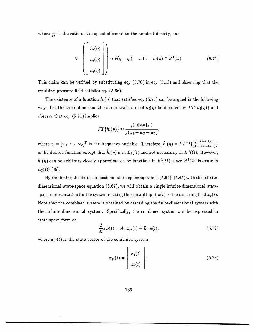
where po is the ratio of the speed of sound to the ambient density, and
hi~n
V. hi(n) z 6 (77- i) with
This claim can be verified by substituting eq. (5.70) in
resulting.pressure field satisfies eq. (5.66).
The existence of a function hi(r) that satisfies eq. (5
way. Let the three-dimensional Fourier transform of hi
observe that eq. (5.71) implies
hi(V) H(Q). (5.71)
eq. (5.13) and observing that the
.71) can be argued in the following
(r/) be denoted by FT{hi(r)} and
e- [w,ni]R3)
j(Wl + w2 + w3)'
where w = [wl w 2 w3]T is the frequency variable. Therefore, hi() =FT- '{j(-j-iR3)
is the desired function except that hi(r) is in £2(Q) and not necessarily in Hl(Q). However,
hi(V) can be arbitrary closely approximated by functions in H 1 (fQ), since H1 (Q) is dense in
L2(Q) [39].
By combining the finite-dimensional state-space equations (5.64)- (5.65) with the infinite-
dimensional state-space equation (5.67), we will obtain a single infinite-dimensional state-
space representation for the system relating the control input u(t) to the canceling field xp(t).
Note that the combined system is obtained by cascading the finite-dimensional system with
the infinite-dimensional system. Specifically, the combined system can be expressed in
state-space form as:
(5.72)dxpl(t) = Aplxpl(t) + Bpju(t),
where xp1(t) is the state vector of the combined system
pI(O = XP(t)
L xl(t) ](5.73)
136

the linear operator ApI is defined as
F XP AP BC1 1 XP 1
XIJ I 0 Al x x
D(ApI) = 1xp IX e D(Ap) and x e R}
and Bx is a bounded linear operator from R into (H x R) defined asand Bvt is a bounded linear operator from R 1 into (H x R n) defined as
[0BPIy =
[Blyj
(5.74)
(5.75)
(5.76)Vy E R1.
It remains to be shown that operator ApI is an infinitesimal generator of a strongly contin-
uous semigroup in an appropriate Hilbert space. The appropriate Hilbert space in this case
is
H' = H x R n, (5.77)
where H is defined in equation (5.19), and the inner product on H' is defined as
[P YPK: : '[ IH= [x YP]H + [l, Y]Rn. (5.78)
Let Tl(t) denote the strongly continuous semigroup generated by Al, and let Tp(t) denote
the strongly continuous semigroup generated by Ap. We claim that operator A is the
infinitesimal generator of the strongly continuous semigroup Tpl(t) defined as
| =| Tp(t)xp + T(t - s)BCITI(s)xlds e
xti I TI(t)xl X
(5.79)
Note that for a fixed t and a fixed x, the integral in (5.79) is a Riemann integral, since
ITp(t - s)BCITj(s)lI is bounded and Tp(t- s)BCITI(s)xl is a continuous function of s.
137
.-- - -- ------- -~~~~ -------
;
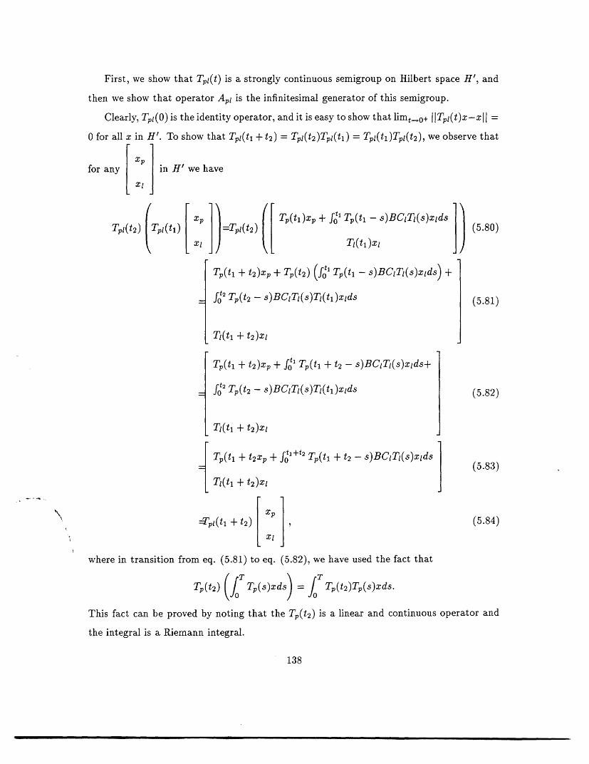
First, we show that Tpl(t) is a strongly continuous semigroup on Hilbert space H', and
then we show that operator Apt is the infinitesimal generator of this semigroup.
Clearly, Tpt(O) is the identity operator, and it is easy to show that limt_0+ [ITpl(t)x-xj =
0 for all x in H'. To show that Tpl(tl + t2) = Tp1(t2)Tp1(tl1 ) = Tp(tl1 )TpI(t 2), we observe that
xpfor any in H we have
Xl
1xp =Tp1( 2 ([ Tp(tl)xp + f;o Tp(t - s)BCIT(s)xIds 1Xl ) Ti(tj)X )
Tp(tl + t2 )Xp + Tp(t2 ) (ot Tp(t1 - s)BCiTi(.s)xids) +
f Tt2 - s)BCjTi(s)Tj(t1 )x lds
T1(t + t 2)XI
Tp(tl + t 2 )xp + ft1 Tp(tl + t2 - s)BCiTl(s)xlds+
f 2 Tp(t 2 - s)BCT(s)Tl(tl )xlds
Tl(tl + t 2)xl
ITp(tl + t 2xp + ftl+t2 Tp(tl + t 2 - s)BCiTl(s)xlds
Tl(tl + t 2)Xl
=Tpl(tl + t2) T ,XI
(5.81)
(5.82)
(5.83)
(5.84)
where in transition from eq. (5.81) to eq. (5.82), we have used the fact that
Tp(t 2 ) (f Tp(s)xds) = I Tp(t2 )Tp(s)xds.
This fact can be proved by noting that the Tp(t 2) is a linear and continuous operator and
the integral is a Riemann integral.
138
Tpl(h) Tpl(tl)

Similarly, we can show that Tpl(tl)Tpl(t 2) = Tpl(tl + t 2). Hence, Tpl(t) is a strongly
continuous semigroup in the Hilbert space H'. We now show that operator Apl is the
infinitesimal generator of the semigroup Tpl(t). To this end, take any in H and
Xl
observe that
XP
Alim
A--B+o
XlPTP()Ap--p + _ fA Tp(t - s)BCiTl(s)xlds
= lim A AA-O+ T(A)xL-xl
A
[F.Axp + BCx1
A xl
L Al
Xp
LXI
(5.85)
(5.86)
L[ X J
(5.87)
Combined State-Space Representation for the Unwanted Noise Field and the
Canceling Field
A single state representation for the acoustic field in fQ is derived in this Section by combining
the state-space representation for the unwanted noise field and the state-space representa-
tion for the canceling field.
We propose the following state-space representation for the acoustic field in Q:
d dtxc(t) = Acxc(t) + Bo(t)u(t) + Fw(t),
where x(t) is the state vector
(t) [ Xd(t)x(t) = t) i
Xpi(i)J
(5.88)
(5.89)
139

Ac is a linear operator on Hilbert space Hc = H x H'
Xd | Ad 0 [d]AC
pl 0 ApL Xpl
[FXdVD(Ac) = Id E D(Ad) and Xp E D(Ap);
Xp'
Bc is a bounded linear operator from R 1 into HC
0By = Vy R,
Bply
FC is a bounded linear operator from H into Hc
(5.90)
(5.91)
(5.92)
FCz = 0 Vz E H. (5.93)
L 0
Next, we show that operator A, is an infinitesimal generator of a strongly continuous
semigroup on Hilbert space H,. To this end, let Tc(t) denote the following family of linear
operators mapping H, into H,:
T(t) d Td(t)d d H. (5.94)
Pl Tpz(t)xpL xpl
We claim that T,(t) is a strongly continuous semigroup on HC, and that operator Ac is the
infinitesimal generator of this semigroup.
Using the fact that Td(t) and Tpl(t) are both strongly continuous semigroups, it is easy
to show that that T¢(t) is a strongly continuous semigroup on Hc. To show that Ac is the
140

Xd 1infinitesimal generator of Tc, we take any in HC and observe that
xpl
Xd Xdr ( 151)__ __
TC(/\) xpl_ xpl: Td(A)Xd-Xd
lim = lim I(5.95),A-.o+ A A-0+ Tp (A)xz1- -xPl
A
AdXd
=I~~~~ ~(5.96)Aplzpl
= c V[ d E H'. (5.97)XP xpl
Observation Process
In a practical active noise cancellation system, the observed signal y(t) is most likely the
output of a microphone. A simple model relating the output of a pressure microphone to
the acoustic field surrounding it is
m(t) = / p(t, r)g(7r)dr + v(t), (5.98)
where m(t) is the output of the microphone at time t; p(t, y) is the pressure field in at
time t; g(rl) is a weighting function in H1 (Q); and v(t) is white measurement noise, uncor-
related with all other processes involved. The region of support of g(77) is the surface of the
diaphragm of the pressure microphone. In this model, the output of the microphone with-
out the measurement noise) is proportional to the weighted integral of the pressure exerted
at the diaphragm of the microphone. This model implicitly assumes that the presence of
the microphone does not alter the acoustic field in fQ, and that the frequency response of
the microphone is constant over those frequencies for which fA p(t, r)g(rl)drj has significant
energy.
141
Recalling that the first component of xd(t) is the unwanted pressure field at time t, and
that the first component of the xl(t) is the canceling pressure field, we see that y(t) can
be expressed in terms of the state-vector xc(t) as
y(t) = Ccxc(t) + Gcw(t) (5.99)
L[ Xd(t) x~t(t)1+c t)(50)where Cc is a linear bounded operator form H' into R 1 , and Gc is a bounded linear operator
form H into R 1, with
GCGc* = Identity, (5.101)
and
FcG* = 0. (5.102)
Note that eq. (5.101) ensures that the measurement noise Gcw(t) is white, and eq. (5.102)
ensures that the measurement noise Gcw(t) is uncorrelated with the process noise Fcw(t).
The explicit operator Cc that results from the microphone model in eq. (5.98) is
Xd XdCC C = [(xd + ),g(7r)]L2 V E H:, (5.103)
Zpl Xpl
where d E H and xp E H'; and x is the first component of d and x is the first
component of xpl. So defined, operator Cc is clearly linear and bounded, since the inner
product operation is linear and bounded.
Optimal Feedback Controller
The governing equations of the acoustic system in Fig. 5.2 can be expressed in state-space
form as
dyx(t) = ACxc(t) + Bcu(t) + Fcw(t) (5.104)
y(t) = cxc(t) + GCw(t). (5.105)
142
The noise cancellation problem is to generate the control signal u(t), based on the observa-
tions of y(t), so that the sum of the acoustic energy in n and the power expended by the
control signal is minimized. Specifically, the cost functional to be minimized is
T T= E{Q(xd(t) + Xp(t))112}dt + j E{Iu(t)112}dt, (5.106)
where Q is bounded linear operator mapping H into H. According to eq. (5.41), (Xd(t) + Xp(t)) KHis the total acoustic energy in the enclosure at time t. Hence, IIQ(xd(t) + xp(t))112 is the
weighted acoustic energy in the enclosure at time t.
The cost function J in eq. (5.106) can be expressed in terms of the state vector xc(t) as
o T= jX E{[JQcXc(t)I 1 }dt + E{uI I(t)112}dt, (5.107)
where Qc is a linear bounded operator from HC into HC defined as
Xd Xd
Q, XP Q(xd + Xp) V P E Hc, (5.108)
Xl Xl
with d E H, xp E H, and x E R n.
From eq. (5.54) we see that for this problem, a unique optimal control uo(t) exists and
can be expressed in feedback form as
u(t) = -B-K(t)ic(t),
where the linear operator K(t) satisfies
d [K(t)x, y] = -[Q*Qcx, y] - [K(t)x, Acy] - [K(t)Acx, y] (5.109)
+[K(t)BcB*K(t)x, y] K(T) = 0, Vx, y e (Ac),
and
c(t, w) = E(xc(t, w) y(s, w) 0 s t).
Furthermore, c(t, w) is calculated using a Kalman filter, i.e.
dxc(t, w) = Aci(t, w) + Pf(t)C*(y(t, w) - CCc(t, w)) + Bcu(t, w) ic(O, w) = 0,
143

where
Pf (t) = E((xc(t, w) - C(t, w))(xc(t, w) - iC(t, w))*),
and Pf (t) satisfies
-[Pf(t)x,y] = [Pf(t)Acx, y] + [Pf(t)x, Acy] + [FcF x,y] (5.110)di
-[Pf(t)C:CcPf(t)x,y] Pf (O) = A x, y E D(A).
An identical derivation can be carried out for the case in which the boundary F of the
enclosure is purely absorbing, i.e. eq. (5.16) is satisfied at the boundary in Fig. 5.2.
5.7 Summary
The distributed active noise cancellation problem was studied in this chapter. We focused
on minimizing the total acoustic energy in an enclosure. To minimize this acoustic energy,
the interaction between the primary field and the canceling field at every point in the
enclosure needed to be considered. The acoustic wave equation was therefore utilized to
model this interaction. The resulting governing equations for the acoustic system were put
in the frame work of infinite-dimensional stochastic linear systems. Using this frame work,
we then derived an optimal feedback controller for attenuating the total acoustic energy in
the enclosure.
The main contribution of this chapter is showing concretely that under certain assump-
tions the distributed ANC problem can be put in the frame work of distributed linear
control. Based on physical models for the canceling loudspeaker and the acoustic field in
the enclosure, a set of coupled ordinary and partial differential equations relating the con-
trol signal to the canceling field were derived. We then showed that these equations can
be represented as abstract differential equations in an appropriate Hilbert space. This rep-
resentation was derived by proving that certain operators were infinitesimal generators of
strongly continuous semigroups.
The primary field was modeled as the state of an infinite-dimensional linear system
driven by a white process. The residual field in the enclosure was modeled as the sum of
this primary field and the canceling field. Based on a physical model for the measurement
144

microphone, we showed that the microphone output could be expressed as a linear function
of the residual field.
We showed that the distributed active noise cancellation problem in an enclosure with
perfectly reflecting or perfectly absorbing boundaries can be put in the above frame work,
provided that the canceling loudspeaker is modeled as a collection of point sources of pres-
sure, and the microphones are modeled by eq. (5.98). In our formulation, the control
signal is pointwise and is used to drive an ordinary loudspeaker, and the observed signal is
pointwise and is obtained as the output of an ordinary pressure microphone. Specifically,
our formulation was used to find the feedback controller that minimizes the distributed
performance criterion J that was defined in eq. (5.106). More precisely, this performance
criterion involves the sum of the acoustic energy in the enclosure and the power expended
by the control signal.
The formulation in this chapter is the first mathematically rigorous formulation of the
distributed active noise cancellation problem known to us. However, this formulation needs
to be extended to the case in which the boundary conditions are more general.
145

Chapter 6
Conclusions and Future Directions
This thesis dealt with the design of optimal feedback controllers for active noise cancellation.
We applied optimal feedback control theory and considered pointwise noise cancellation as
well as distributed noise cancellation. By formulating the ANC problem as an optimal feed-
back control problem, we developed a single approach for designing controllers for pointwise
and distributed active noise cancellation.
The key strategy is to model the residual signal/field as the sum of the outputs of two
linear systems. The unwanted noise signal/field is modeled as the output of a linear system
driven by a white process. Similarly, the canceling signal is modeled as the output of another
linear system driven by the control signal. Finally, the residual signal/field is modeled as
the sum of the outputs of these two linear systems. These two models are combined to
represent the overall acoustic system as a single linear system driven by a control process
and a white noise process. We showed that the optimal control signal is a linear feedback
of the estimated states of this overall system. These state estimates are computed using a
Kalman filter, and the feedback gain is obtained from a Riccati equation. Note that in the
pointwise case and the distributed case, the control signal is not distributed and is used to
drive an ordinary loudspeaker. Moreover, in both these cases, the control signal is generated
based on the outputs of ordinary microphones.
While we focused specifically on the acoustic noise cancellation problem, the results
developed in this thesis can be applied to other active cancellation problems. Vibration
146
control is an example of a non-acoustic problem to which our results can be applied.
6.1 Summary and Contributions
We started by developing an optimal feedback controller for attenuating the acoustic pres-
sure at the locations of a finite number of microphones. The error microphones are placed
at those locations where noise attenuation is desired, and the canceling loudspeaker is
placed in the vicinity of these microphones. We model the residual signals at the micro-
phones as the sum of the outputs of two finite-dimensional linear systems. The unwanted
noise signals at the microphones are modeled as the outputs of a multiple-input/multiple-
output finite-dimensional linear system driven by a white process. This finite-dimensional
system provides a compact representation for the second-order statistics of the unwanted
signals. Similarly, the canceling signals at the microphones are modeled as the outputs of a
single-input/multiple-output finite-dimensional linear system driven by the control signal.
This linear system corresponds to the matrix of transfer functions from the input to the
loudspeaker to the canceling signals at microphones. Finally, the residual signals at the
microphones are modeled as the sum of the outputs of these two finite-dimensional linear
systems. These two linear system models are then combined to represent the overall acous-
tic system as a single finite-dimensional linear system driven by a control process and a
white noise process.
We showed that a certain class of performance criterion involving the mean-square sum
of the residual signals and the mean-square sum of the control signal could be expressed as a
quadratic form in the state of the overall system and in the control signal. The control signal
that minimizes this performance criterion is found to be a linear feedback of the estimated
states of the overall system. These state estimates can be computed using a Kalman filter,
and the control gain can be computed by iterating a Riccati matrix equation. We also
showed that the same formulation can be used to minimize the frequency weighted power
of the residual signal. Such a frequency dependent weighting might be important because
of the difference in the sensitivity of the ear to sounds at different frequencies.
Our pointwise feedback controller has a few important advantages compared to existing
147
feedback controllers for ANC. Recall that analog feedback controllers (e.g., [51]) do not take
advantage of the statistics of the noise. However, our feedback controller takes full advantage
of the statistical characteristics of the noise. The discrete-time single-microphone feedback
controller proposed by Graupe [26] can not be used in the case that the plant model contains
one or more delays. However, the feedback controller developed in this thesis can be used
in this case. Furthermore, the feedback controller developed in this thesis can be used in
the single-microphone as well as multiple-microphone configuration.
Our pointwise feedback controller achieves the same acoustic objective as the existing
multiple-channel feedforward controllers for ANC, without the problems associated with
acquiring an appropriate reference signal that is commonly experienced by feedforward
controllers.
A few experiments were presented to illustrate the performance of the optimal point-
wise feedback controller in the context of aircraft noise. The optimal feedback controller
outperformed the feedforward controller proposed by Burgess by about 10dB. Similarly,
the hardware implementation of the optimal feedback controller outperformed an analog
feedback controller by about 9dB.
In the context of distributed active noise cancellation, we focused on developing an
optimal feedback controller for attenuating the total acoustic energy in an enclosure. The
distributed ANC system utilizes one microphone to monitor the residual field and one
loudspeaker to generate the canceling field. The control signal driving the loudspeaker
must be generated based solely on the microphone output. To minimize the total acoustic
energy in the enclosure, the interaction between the canceling field and the unwanted noise
field at every point in the enclosure needs to be considered.
The residual field in the enclosure is modeled as the sum of the outputs of two infinite-
dimensional linear systems. The unwanted noise field is modeled as the output of an infinite-
dimensional linear system driven by a white process. This infinite-dimensional system
provides a compact representation for the second-order statistics of the unwanted noise
field. Similarly, the canceling field in the enclosure is modeled as the output of another
infinite-dimensional linear system driven by the input to the loudspeaker. We showed that
148
this model can accommodate the finite-dimensional dynamics of the loudspeaker as well as
the infinite-dimensional acoustical dynamics of the enclosure, provided that the loudspeaker
is modeled as a collection of point sources of pressure and the boundary surrounding the
enclosure is perfectly absorbing or perfectly reflecting. This was shown by proving that a
certain operate was an infinitesimal generator of a strongly continuous semigroup.
We then illustrated that the linear system representation of the unwanted noise field
and the linear system representation of the canceling field can be combined to represent
the overall acoustic system as a single infinite-dimensional linear system driven by a control
process and a white noise process. Again, this was illustrated by proving that a certain
operator was an infinitesimal generator of a strongly continuous semigroup.
Next, we showed that the microphone output at time "t" can be expressed as a linear
functional of the state of the overall system at time "t". This was shown based on a physical
model for a pressure microphone suggested in [6].
Finally, we considered a class of performance criterion involving the sum of the total
acoustic energy in the enclosure and the power expended by the control signal. We demon-
strated that this performance criterion can be expressed as the expected value of a quadratic
form in the state of the overall system and in the control signal. The control input that
minimizes this performance criterion is a linear feedback of the estimated states of the over-
all system. These state estimates can be computed using a Kalman filter, and the feedback
gain can be computed form a Riccati operator equation.
Our results for the distributed ANC problem are important because they are the first
mathematically rigorous formulation of the distributed ANC problem. Furthermore, it has
been demonstrated in numerical studies that attenuation of noise at a finite number of
spatial points can result in amplification of the noise at other points [15].
Comparing our formulation of the pointwise ANC problem to our formulation of the
distributed ANC problem, we see the fundamental importance of being able to represent
the acoustic system as a linear system driven by a control process and a white noise pro-
cess. Similarly, to use this formulation, it is essential that the performance criterion be
an expected value of a quadratic form in the state of this linear system and in the control
149

process. In the pointwise case, it was straight forward to represent the acoustic system in
this form; however, in the distributed case, rather sophisticated mathematical machinery
was needed to represent the overall acoustic system in this form.
Several recursive/adaptive algorithms for modeling the unwanted noise at a single micro-
phone were developed in Chapter 4. We assumed that the unwanted noise at the microphone
is the output of an all-pole transfer function driven by a white process and develop a re-
cursive/adaptive algorithm for estimating the parameters of this transfer function based
on the measurements made by the microphone. An adaptive feedback ANC system can
be obtained by combining the pointwise optimal control law with these recursive/adaptive
algorithms for modeling the unwanted noise. Note that the resulting adaptive controller
only adapts to changes in the noise statistics and not to changes in the plant. Although we
focused specifically on developing estimation algorithms for modeling the unwanted noise
in the ANC problem, the algorithms presented in Chapter 4 can be applied to the more
general problem of identifying non-stationary autoregressive (AR) processes embedded in
white noise.
6.2 Future Directions
We foresee several immediate branches down which the work in this thesis may continue.
Developing adaptive optimal feedback controllers for pointwise ANC is a potentially
promising area for future work. Our derivation of the optimal pointwise feedback con-
troller was based on the assumption that the noise model and the plan model were known.
However, in some applications both the plant characteristics and the unwanted noise char-
acteristics might be unknown or changing. By properly combining an adaptive parameter
estimation algorithm with the control law developed in Chapter 3, an adaptive optimal
feedback controller for ANC can be obtained. Adaptive optimal control is a mature field,
and many of the results developed in this field should be directly applicable here.
Our results for the distributed ANC problem were derived for enclosures with perfectly
reflecting or perfectly absorbing boundaries. Extending these results so that they apply
to enclosures with more general boundary conditions would be very useful. In the more
150
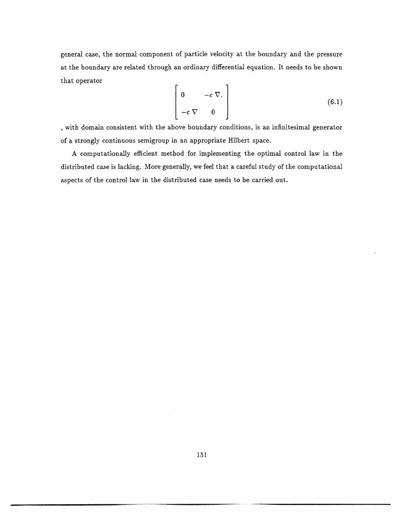
general case, the normal component of particle velocity at the boundary and the pressure
at the boundary are related through an ordinary differential equation. It needs to be shown
that operator
0 - V.(6.1)
-cV 0
, with domain consistent with the above boundary conditions, is an infinitesimal generator
of a strongly continuous semigroup in an appropriate Hilbert space.
A computationally efficient method for implementing the optimal control law in the
distributed case is lacking. More generally, we feel that a careful study of the computational
aspects of the control law in the distributed case needs to be carried out.
151
---

Bibliography
[1] R.A. Adams, Sobolev Spaces, N.Y., Academic Press, 1975.
[2] K. Astrom and B. Wittenmark, Computer Controlled Systems: Theory and Design,
Englewood Cliffs, N.J., Prentice-Hall 1984.
[3] M. Athans and P. Falb, Optimal Control: an introduction to the theory and applications,
N.Y., McGraw-Hill, 1966.
[4] O.L. Angevine, "Active Acoustic Attenuation of Transformer Noise," Proc. Inter-
noise81, 1981.
[5] A.V. Balakrishnan, Applied Functional Analysis, New York: Springer-Verlag, 1981.
[6] Leo. L. Beranek, Acoustics, McGraw-Hill, 1954.
[7] M. Berengier and A. Roure, "Broad-Band Active Sound Absorption in a Duct Carrying
Uniformly Flowing Fluid," Journal of Sound and Vibration 68, 1980.
[8] G. Box and G. Jenkins, Time Series Analysis, Forecasting and Control, San Francisco,
CA: Holden Day, 1970.
[9] A.J. Bullmore, P.A. Nelson, A.R.D. Curtis, and S.J. Elliot, "The Active Minimization
of Harmonic Enclosed Sound Fields, Part II," Journal of Sound and Vibration 117,
1987.
[10] A. Burgess, "Active adaptive sound control in a duct: A computer simulation" Journal
of the Acoustical Society of America, Vol 70, No. 3, pp. 715-726, September, 1981.
152

[11] G. Canevet, "Active Sound Absorption in an Air Conditioning Duct," Journal of Sound
and Vibration 58, 1987.
[12] C. Carme, Absorption acoustique active dans les cavites, Ph.D. Thesis, Universite
D'Aix-Marseille II, 1987.
[13] G.B. Chaplin, "Method and Apparatus for canceling Vibration," U.S. Patent Number
4,489,441 December 18, 1984
[14] A.R.D. Curtis, P.A. Nelson, S.J. Elliot, and A.J. Bulmore, "Active Suppression of
Acoustic Resonance," Journal of Acoustical Society of America, 1987.
[15] A. David and S.J. Elliot, "Numerical Studies of Actively Generated Quiet Zones,"
Applied Acoustics, 1993.
[16] A.P. Dowling and J.E. Ffowcs Williams, Sound and Sources of Sound, New York: John
Wiley and Sons
[17] J.E. Efowcs Williams, I. Roebuk, and C. Ross, "Anti Phase Noise Reduction," Physical
Technology, 16.
[18] S.J. Elliot, I.M. Stothers, and P.A. Nelson, "A Multiple Error LMS Algorithm and Its
Application to the Active Control of Sound and Vibration," IEEE Trans. ASSP, VOL.
ASSP-35, 1987.
[19] S.J. Elliot, A.R.D. Curtis, A.J. Bullmore, and P.A. Nelson, "The Active Minimization
of Harmonic Enclosed Sound Fields, Part III," Journal of Sound and Vibration 117,
1987.
[20] S.J. Elliot, C.C. Boucher, and P.A. Nelson, "The Behavior of a Multiple Channel Active
Control System," IEEE Trans. Signal Processing, VOL. 40, NO. 5, 1992.
[21] S.J. Elliot and P.A. Nelson, "Algorithm for Multichannel LMS Adaptive Filtering,"
Electronics Letters, VOL. 21, NO. 21, 1985.
153
]

[22] S.J. Elliot, P. Joseph, A.J. Bullmore, and P.A. Nelson, "Active Cancellation of a Point
Pure Tone Diffuse Sound Field," Journal of Sound and Vibration 120, 1988.
[23] L.J. Eriksson, M.C. Allie, and C.D. Bremigan, "Active Noise Control Using Adaptive
Digital Signal Processing," Proc. ICASSP, New York, 1988, pp. 2594-2597.
[24] Franklin, Powell, and Workman, Digital Control of Dynamic Systems, Addison-Welsely,
1990.
[25] D.C. Gilliland, "Sequential Compound Estimation," Annual Mathematical Statistics,
Vol. 39, No. 6, pp 1890-1904, 1968.
[26] D. Graupe and A. Efron, "An Output-Whitening Approach to Adaptive Noise Cancel-
lation," IEEE Trans. Circuits and Systems, Vol. 38, No. 11, November 1991.
[27] D. Guicking, Active Noise and Vibration Control: Reference Bibliography, 1991, Uni-
versity of Gottingen, West Germany.
[28] M.J.M. Jessel, "La question des absorbeurs activs," Revue d'acoust 37, 1972.
[29] M.J.M. Jessel and O.L. Angevine, "Active Acoustic Attenuation of a Complex Noise
Source," Inter Noise80, December 1980.
[30] M.J.M Jessel and G.A. Mangiante, "Active Sound Absorbers in an Air Duct," Journal
of Sound and Vibration 23, 1972.
[31] A.J. Kempton, "The Ambiguity of Acoustic Sources-a Possibility for Active Control,"
Journal of Sound and Vibration 48, 1976.
[32] K. Kido, "Reduction of Noise by Use of Additional Sources," Proc. Internoise75, 1975.
[33] E. Kreyszig, Introductory Functional Analysis with Applications, New York: Wiley and
Sons, 1978.
[34] R.C. Lee, Optimal Estimation, Identification, and Control, MIT Press, Cambridge,
1964.
154

[35] J.S. Meditch, Stochastic Optimal Linear Estimation and Control, McGraw-Hill, N.Y.
1969.
[36] P.A. Nelson, A.R.D. Curtis, S.J. Elliot, and A.J. Bullmore, "The Active Minimization
of Harmonic Enclosed Sound Fields, Part I," Journal of Sound and Vibration 117,
1987.
[37] Nelson, Curtis, Elliot, and Bullmore, "The Minimum Power Output of Free Field Point
Sources and the Active Control of Sound," Journal of Sound and Vibration 117, 1987.
[38] Y. Nogami, "The k-extended set-compound estimation problem in a nonregular family
of distribution over [0, + 1]," Annal Institute of Statistical Mathematics, Vol. 31A, pp.
169-176, 1979.
[39] J.T. Oden, and J.N. Reddy, An Introduction to the Mathematical Theory of Finite
Elements, Wiley and Sons, 1976.
[40] A. Oppenheim, E. Weinstein, K. Zangi, M. Feder, and D. Gauger, "Single Sensor Active
Noise Cancellation Based on the EM Algorithm," Proc. ICASSP, San Francisco, 1992,
Vol. I, pp. 277-280.
[41] J.H.B. Poole and H.G. Leventhall, "An Experimental Study of Swinbanks' Method
of Active Noise Attenuation of Sound in Ducts," Journal of Sound and Vibration 49,
1976.
[42] H. Robbins, "Asymptotically subminimax solutions of compound statistical decision
problems", Proceedings of the 2nd Berkeley Symposium on Mathematical Statistical
Problems, pp. 131-148, 1951.
[43] H. Robbins and S. Monro, "A stochastic approximation method", Annals of Mathe-
matical Statistics, 22:400-407, 1951.
[44] C. F. Ross, "A Demonstration of Active Control of Broadband Sound," Journal of
Sound and Vibration 74, 1981.
155
----

[45] J. Van Ryzin, "The sequential compound decision problem with m x n finite loss
matrix," Annual Mathematical Statistics, Vol. 37, pp. 954-975, 1966.
[46] S.D. Snyder and C.H. Hansen, "Active Noise Control in Ducts: Some Physical In-
sights," Journal of Acoustic Society of America, 1989.
[47] S. D. Snyder and C. H. Hansen, "Design Considerations for Active Noise Control
Systems Implementing the Multiple Input, Multiple Output LMS Algorithm," Journal
of Sound and Vibration 159, 1992.
[48] S. D. Snyder and C. H. Hansen, "The Influence of Transducer Transfer Function and
Acoustic Delays on the Implementation of the LMS Algorithm in Active Noise Control
Systems," Journal of Sound and Vibration 141, 1990.
[49] M.A. Swinbanks, "Active Control of Sound Propagation in Long Ducts," Journal of
Sound and Vibration 27, 1973.
[50] G.E. Warnaka, L. Poole, and J. Tichy, "Active Attenuator," US Patent Number
4,473,906 September 25, 1984.
[51] B. Wheeler, Voice Communication in the cockpit noise environment- the role of active
noise reduction, Ph.D. Thesis, University of Southampton, England, 1986.
[52] B. Widrow et al., "Adaptive noise canceling: principles and applications," Proc. IEEE,
Vol. 63, No. 12, December 1975.
[53] B. Widrow and S.D. Stearns, Adaptive Signal Processing, Prentice Hall, Englewood
Cliffs, NJ 1985.
[54] S.B. Vardeman, "Admissible solutions of k-Extended finite state set and sequence com-
pound decision problems," Journal of Multivariate Analysis, Vol. 10, pp 426-441, 1980.
[55] E. Weinstein, A. Oppenheim, K. Zangi, M. Feder, and D. Gauger, "Single-Sensor Active
Noise Cancellation," IEEE Trans. Audio Processing April 1994.
156

[56] E. Weinstein, M. Feder, and A. Oppenheim, "Signal Enhancement Using Single and
Multiple-Sensor Measurements," MIT-RLE Technical Report No. 560, December 1990.
[57] N. Wiener, Extrapolation, Interpolation, and Smoothing of Stationary Time Series,
with Engineering Applications, New York: Wiley, 1949.
[58] P.E. Wellstead and M.B. Zarrop, Self-tuning Systems: Control and Signal Processing,
Chichester, N.Y, Wiley, 1991.
[59] K.C. Zangi, "A New Two Microphone Active Noise Cancellation Algorithm," Proc.
ICASSP 1993, Minneapolis, Vol. II, pp. 351-354, April 1993.
157