optimal design strategies for survivable carrier …

OPTIMAL DESIGN STRATEGIES FOR

SURVIVABLE CARRIER ETHERNET NETWORKS

MOHAMMAD NURUJJAMAN

A THESIS

IN

THE DEPARTMENT

OF

COMPUTER SCIENCE & SOFTWARE ENGINEERING

PRESENTED IN PARTIAL FULFILLMENT OF THE REQUIREMENTS

FOR THE DEGREE OF DOCTOR OF PHILOSOPHY

CONCORDIA UNIVERSITY

MONTREAL, QUEBEC, CANADA

APRIL 2013

c© MOHAMMAD NURUJJAMAN, 2013

CONCORDIA UNIVERSITY

Engineering and Computer Science

This is to certify that the thesis prepared

By: Mohammad NurujjamanEntitled: Optimal Design Strategies for Survivable Carrier Eth-

ernet Networksand submitted in partial fulfillment of the requirements for the degree of

Doctor of Philosophy (Computer Science)

complies with the regulations of this University and meets the accepted stan-dards with respect to originality and quality.

Signed by the final examining committee:

Dr. Rabin RautChair

Dr. Pin-Han HoExternal Examiner

Dr. Anjali AgarwalExternal to Program

Dr. Lata NarayananExaminer

Dr. Thomas G. FevensExaminer

Dr. Chadi AssiThesis Supervisor

Approved by

———————————————————————–Chair of Department or Graduate Program Director

—————— ——————————————Date Dean of Faculty

AbstractOptimal Design Strategies for Survivable Carrier Ethernet

Networks

Mohammad Nurujjaman, Ph.D.

Concordia University, 2013

Ethernet technologies have evolved through enormous standardization efforts

over the past two decades to achieve carrier-grade functionalities, leading to

carrier Ethernet. Carrier Ethernet is expected to dominate next generation

backbone networks due to its low-cost and simplicity. Ethernet’s ability to

provide carrier-grade Layer-2 protection switching with SONET/SDH-like fast

restoration time is achieved by a new protection switching protocol, Ethernet

Ring Protection (ERP). In this thesis, we address two important design aspects

of carrier Ethernet networks, namely, survivable design of ERP-based Ether-

net transport networks together with energy efficient network design. For the

former, we address the problem of optimal resource allocation while designing

logical ERP for deployment and model the combinatorially complex problem of

joint Ring Protection Link (RPL) placements and ring hierarchies selection as

an optimization problem. We develop several Mixed Integer Linear Program-

ming (MILP) model to solve the problem optimally considering both single link

failure and concurrent dual link failure scenarios. We also present a traffic en-

gineering based ERP design approach and develop corresponding MILP design

models for configuring either single or multiple logical ERP instances over one

underlying physical ring. For the latter, we propose two novel architectures of

energy efficient Ethernet switches using passive optical correlators for optical

iii

bypassing as well as using energy efficient Ethernet (EEE) ports for traffic ag-

gregation and forwarding. We develop an optimal frame scheduling model for

EEE ports to ensure minimal energy consumption by using packet coalescing

and efficient scheduling.

iv

Acknowledgments

I would like to express my sincere gratitude to my thesis supervisor, Dr. Chadi

Assi, who is very hard working, dedicated and extremely helpful to his stu-

dents. It would have been impossible for me to accomplish this endeavor with-

out his encouragement, constant support and guidance.

I collaborated with several scholars and researchers in the field of optimiza-

tion and communication networks throughout my PhD. I’d also like to express

my appreciation to Dr. Samir Sebbah, Dr. Hamed Alazemi, Dr. Ahmad Khalil

and Dr. Mohammad F. Uddin for their active collaboration which yielded to

authoring high-quality and well received journal and conference papers. Fur-

thermore, I was granted a warm and friendly atmosphere in our research lab

at Concordia University throughout my PhD. I am greatly thankful to all of

my colleagues.

I also appreciate the funding support from the Fonds De Recherche du

Quebec- Nature et Technologies (FQRNT) and Natural Sciences and Engineer-

ing Research Council of Canada (NSERC).

My deepest appreciation goes to my loving wife. Aside from myself, no one

has been more impacted than her by this dissertation. I would like to thank

her for all her support, constant love and care. Finally, I am grateful to my

parents. I could never achieve my ambitions without their encouragement,

understanding, support and true love.

v

Contents

List of Figures x

List of Tables xiii

1 Introduction 1

1.1 Motivation . . . . . . . . . . . . . . . . . . . . . . . . . . . . . . . . 1

1.2 Objectives . . . . . . . . . . . . . . . . . . . . . . . . . . . . . . . . 5

1.3 Contributions & Outline . . . . . . . . . . . . . . . . . . . . . . . . 6

2 Metro Ethernet Fundamentals and Related Work 9

2.1 Native Ethernet & limitations . . . . . . . . . . . . . . . . . . . . . 9

2.2 Why Ethernet as Carrier? . . . . . . . . . . . . . . . . . . . . . . . 10

2.3 Evolution of Carrier Ethernet . . . . . . . . . . . . . . . . . . . . . 11

2.3.1 Standardized Services . . . . . . . . . . . . . . . . . . . . . 12

2.3.2 Scalability . . . . . . . . . . . . . . . . . . . . . . . . . . . . 16

2.3.3 Reliability . . . . . . . . . . . . . . . . . . . . . . . . . . . . 21

2.3.4 Service Management . . . . . . . . . . . . . . . . . . . . . . 22

2.3.5 Quality of Service . . . . . . . . . . . . . . . . . . . . . . . . 24

2.4 Ethernet Ring Protection (ERP) . . . . . . . . . . . . . . . . . . . . 24

2.4.1 Characteristics of ERP Architectures . . . . . . . . . . . . . 27

2.4.2 Principles of ERP operations . . . . . . . . . . . . . . . . . 30

vi

2.5 Related work . . . . . . . . . . . . . . . . . . . . . . . . . . . . . . . 33

3 Design of ERP: Single Failure 38

3.1 Ethernet Ring Protection: A Primer . . . . . . . . . . . . . . . . . 39

3.2 ERP Design perspectives . . . . . . . . . . . . . . . . . . . . . . . . 42

3.2.1 Single stand-alone ring . . . . . . . . . . . . . . . . . . . . . 42

3.2.2 Mesh of interconnected multi-rings . . . . . . . . . . . . . . 46

3.3 Limitations of related work and resolutions . . . . . . . . . . . . . 48

3.3.1 Overestimation of capacity provisioning . . . . . . . . . . . 49

3.3.2 Infeasible configurations . . . . . . . . . . . . . . . . . . . . 51

3.3.3 Solutions . . . . . . . . . . . . . . . . . . . . . . . . . . . . . 52

3.4 ILP-based solution methodology . . . . . . . . . . . . . . . . . . . . 53

3.5 Numerical Results . . . . . . . . . . . . . . . . . . . . . . . . . . . . 60

3.6 Chapter remark . . . . . . . . . . . . . . . . . . . . . . . . . . . . . 63

4 Design of ERP: Dual Failures 65

4.1 Two-step approach . . . . . . . . . . . . . . . . . . . . . . . . . . . 66

4.1.1 Characterizing Service Outages in ERP . . . . . . . . . . . 67

4.1.2 Problem Formulation . . . . . . . . . . . . . . . . . . . . . . 74

4.1.3 Numerical results I . . . . . . . . . . . . . . . . . . . . . . . 76

4.1.4 Further Observations . . . . . . . . . . . . . . . . . . . . . . 79

4.2 Joint approach . . . . . . . . . . . . . . . . . . . . . . . . . . . . . . 88

4.2.1 Category - 2 Outages . . . . . . . . . . . . . . . . . . . . . . 89

4.2.2 Illustrative example . . . . . . . . . . . . . . . . . . . . . . 90


4.2.4 Numerical results . . . . . . . . . . . . . . . . . . . . . . . . 102

4.3 Chapter remark . . . . . . . . . . . . . . . . . . . . . . . . . . . . . 108

vii

5 Design of ERP: Traffic Engineering 111

5.1 Traffic engineering over single ERP instance . . . . . . . . . . . . 112

5.1.1 Problem Statement . . . . . . . . . . . . . . . . . . . . . . . 113

5.1.2 Illustrative Example . . . . . . . . . . . . . . . . . . . . . . 114



5.2 Traffic engineering over multiple ERP instances . . . . . . . . . . 122

5.2.1 Operation of multiple ERP instances . . . . . . . . . . . . . 122

5.2.2 Design perspectives using multiple ERP instances . . . . . 123

5.2.3 Problem Statement . . . . . . . . . . . . . . . . . . . . . . . 125

5.2.4 Mapping Problem . . . . . . . . . . . . . . . . . . . . . . . . 126

5.2.5 Illustrative example . . . . . . . . . . . . . . . . . . . . . . 128



5.3 Chapter remark . . . . . . . . . . . . . . . . . . . . . . . . . . . . . 136

6 Green Ethernet Transport Network 138

6.1 GMPLS Ethernet Label Switching (GELS) and open issues . . . . 140

6.1.1 GMPLS Ethernet Label Switching (GELS) . . . . . . . . . 140

6.1.2 Open Issues . . . . . . . . . . . . . . . . . . . . . . . . . . . 142

6.2 Photonic PBB-TE (PPBB-TE) Switches . . . . . . . . . . . . . . . 144

6.2.1 PPBB-TE Core Switch . . . . . . . . . . . . . . . . . . . . . 150

6.2.2 PPBB-TE Edge Switch . . . . . . . . . . . . . . . . . . . . . 152

6.3 Energy-Aware scheduling . . . . . . . . . . . . . . . . . . . . . . . 155

6.3.1 Illustrative Example . . . . . . . . . . . . . . . . . . . . . . 156


6.3.3 Sequential Fixing . . . . . . . . . . . . . . . . . . . . . . . . 161

viii

6.4 Numerical Results . . . . . . . . . . . . . . . . . . . . . . . . . . . . 161

6.4.1 Comparison of MILP with existing approaches . . . . . . . 162

6.4.2 Optimization model and sequential fixing . . . . . . . . . . 165

6.4.3 Impact of frame delay and sizes on the energy consumption165

6.5 Chapter remark . . . . . . . . . . . . . . . . . . . . . . . . . . . . . 168

7 Conclusion and Future Directions 171

7.1 Conclusions . . . . . . . . . . . . . . . . . . . . . . . . . . . . . . . 171

7.2 Future Work . . . . . . . . . . . . . . . . . . . . . . . . . . . . . . . 173

Bibliography 182

ix

List of Figures

2.1 Five attributes of carrier Ethernet [source: [1]] . . . . . . . . . . . 12

2.2 Ethernet Line (E-Line) [source: [1]] . . . . . . . . . . . . . . . . . . 14

2.3 Ethernet LAN (E-LAN) [source: [1]] . . . . . . . . . . . . . . . . . 15

2.4 Ethernet Tree (E-Tree) [source: [1]] . . . . . . . . . . . . . . . . . . 17

2.5 Architectural evolution of Ethernet [source: [2]] . . . . . . . . . . 18

2.6 An example of ERP implementation . . . . . . . . . . . . . . . . . 28

2.7 Failure scenarion in ERP [source: [3]] . . . . . . . . . . . . . . . . 31

2.8 Failure receovery process in ERP [source: [3]] . . . . . . . . . . . . 32

3.1 ERP Operations . . . . . . . . . . . . . . . . . . . . . . . . . . . . . 39

3.2 Illustrative example: A single ring instance . . . . . . . . . . . . . 42

3.3 Illustrative example: Interconnected multi-ring instance 1 . . . . 46

3.4 Illustrative example: Interconnected multi-ring instance 2 . . . . 48

3.5 Capacity provisioning steps . . . . . . . . . . . . . . . . . . . . . . 50

3.6 Loop existence in ARPA2 . . . . . . . . . . . . . . . . . . . . . . . . 52

3.7 ILP vs ExS . . . . . . . . . . . . . . . . . . . . . . . . . . . . . . . . 60

3.8 ILP vs ExS (excluding unnecessary configurations) . . . . . . . . 61

3.9 ILP vs ExS (including additional constraint) . . . . . . . . . . . . 62

4.1 Physical and logical segmentation . . . . . . . . . . . . . . . . . . 68

4.2 Dynamic procedure . . . . . . . . . . . . . . . . . . . . . . . . . . . 69

4.3 Segmentation in a 3-connected network . . . . . . . . . . . . . . . 72

x

4.4 Minimized capacity investment against single-link failure . . . . 73

4.5 Reduced segmentation . . . . . . . . . . . . . . . . . . . . . . . . . 73

4.6 COST239 service outages . . . . . . . . . . . . . . . . . . . . . . . 77

4.7 NSFNET service outages . . . . . . . . . . . . . . . . . . . . . . . . 78

4.8 ARPA2 service outages . . . . . . . . . . . . . . . . . . . . . . . . . 79

4.9 Service outages due to inadequate capacity . . . . . . . . . . . . . 82

4.10 COST239 service outages . . . . . . . . . . . . . . . . . . . . . . . 85

4.11 NSFNET service outages . . . . . . . . . . . . . . . . . . . . . . . . 86

4.12 ARPA2 service outages . . . . . . . . . . . . . . . . . . . . . . . . . 87

4.13 Comparison of network-wide restorability . . . . . . . . . . . . . . 88

4.14 Category-1 and category-2 outages . . . . . . . . . . . . . . . . . . 90

4.15 Illustrative example . . . . . . . . . . . . . . . . . . . . . . . . . . . 92

4.16 Performance Comparison with prior works using COST239 net-

work . . . . . . . . . . . . . . . . . . . . . . . . . . . . . . . . . . . . 104

4.17 Comparison between different design strategies using Random

network . . . . . . . . . . . . . . . . . . . . . . . . . . . . . . . . . . 105

4.18 Comparison between different design strategies using COST239

network . . . . . . . . . . . . . . . . . . . . . . . . . . . . . . . . . . 106

4.19 Comparison of capacity and service outages with varying reward

factor (ρ) in COST239 network . . . . . . . . . . . . . . . . . . . . 107

5.1 Variations of granted flow in different RPL placement . . . . . . . 114

5.2 The impact of ring hierarchy on the amount of granted flow . . . 115

5.3 Net flow in COST239 network . . . . . . . . . . . . . . . . . . . . . 119

5.4 Net flow in NSF network . . . . . . . . . . . . . . . . . . . . . . . . 120

5.5 Fairness in COST239 network . . . . . . . . . . . . . . . . . . . . . 120

5.6 Fairness in NSF network . . . . . . . . . . . . . . . . . . . . . . . . 121

xi

5.7 Logical ERP instances over a single physical ring . . . . . . . . . 124

5.8 Illustrative example . . . . . . . . . . . . . . . . . . . . . . . . . . . 127

5.9 Comparison of total flow/latency . . . . . . . . . . . . . . . . . . . 136

5.10 Comparison of average flow/latency . . . . . . . . . . . . . . . . . . 137

6.1 EEE 802.3az transition policy between Low Power Idle and ac-

tive mode [4]. . . . . . . . . . . . . . . . . . . . . . . . . . . . . . . . 143

6.2 Proposed network architecture with Photonic PBB-TE (PPBB-

TE) edge and core nodes supporting different types of Eth-LSP. . 145

6.3 Architecture of PPBB-TE core switch. . . . . . . . . . . . . . . . . 150

6.4 Hash Table . . . . . . . . . . . . . . . . . . . . . . . . . . . . . . . . 153

6.5 Architecture of PPBB-TE edge switch. . . . . . . . . . . . . . . . . 154

6.6 Scheduling options for a simple instance. . . . . . . . . . . . . . . 157

6.7 Energy consumption vs. link utilization . . . . . . . . . . . . . . . 162

6.8 Energy consumption vs. link utilization . . . . . . . . . . . . . . . 164

6.9 CPU time of OM vs. SF . . . . . . . . . . . . . . . . . . . . . . . . . 166

6.10 Energy consumption of OM vs. SF . . . . . . . . . . . . . . . . . . 167

6.11 Energy consumption with varying delay range . . . . . . . . . . . 168

6.12 Energy consumption with varying frame size . . . . . . . . . . . . 169

6.13 Energy efficiency with varying frame size . . . . . . . . . . . . . . 170

xii

List of Tables

3.1 Comparison of ILP and ExS . . . . . . . . . . . . . . . . . . . . . . 63

4.1 Comparison of Alternative Solutions . . . . . . . . . . . . . . . . . 74

4.2 Capacity trade-off between two approaches . . . . . . . . . . . . . 79

4.3 Capacity trade-off between three approaches . . . . . . . . . . . . 109

4.4 Comparison of Category-1 and Category-2 service outages . . . . 110

6.1 Parameter values . . . . . . . . . . . . . . . . . . . . . . . . . . . . 156

6.2 Avg. delay vs. link utilization . . . . . . . . . . . . . . . . . . . . . 164

xiii

List of Acronyms

SONET Synchronous optical networking

SDH Synchronous Digital Hierarchy

CAPEX Capital Expenditure

OPEX Operational Expenditure

MEF Metro Ethernet Forum

WDM Wavelength Division Multiplexing

LAN Local Area Network

VLAN Virtual Local Area Network

EPL Ethernet Private Line

EVPL Ethernet Virtual Private Line

EP-LAN Ethernet Private LAN

EVP-LAN Ethernet Virtual Private LAN

EP-Tree Ethernet Private Tree

EVP-Tree Ethernet Virtual Private Tree

STP Spanning Tree Protocol

MSTP Multiple Spanning Tree Protocol

RSTP Rapid Spanning Tree Protocol

MPLS Multi Protocol Label Switching

GMPLS Generalized MPLS

LP Linear Programing

xiv

ILP Integer Linear Programing

MILP Mixed Integer Linear Programming

EEE Energy Efficient Ethernet

ERP Ethernet Ring Protection

RPL Ring Protection Link

ESP Ethernet Switched Paths

LSP Label Switched Path

Eth-LSPs Ethernet-LSPs

FDB Filtering Database

ITU-T ITU Telecommunication Standardization Sector

LPI Low Power Idle

PBB-TE Provider Backbone Bridge - Traffic Engineering

PPBB-TE Photonic Provider Backbone Bridge - Traffic Engineering

MAC Medium Access Control

NIC Network Interface Card

NP Nondeterministic Polynomial Time

QoS Quality of Service

s-d Source-Destination

SF Sequential Fixing

xv

Chapter 1

Introduction

1.1 Motivation

Synchronous optical networking/Synchronous Digital Hierarchy (SONET/SDH)

circuit-switched time division multiplexing (TDM) equipments are dominat-

ing the installed infrastructures of today’s backbone networks. Following the

ITU-T’s Global Standards Initiative (GSI), the current widely deployed circuit-

switching SONET/SDH networks will evolve into Next Generation Networks

(NGNs) whose data transfer is based on packets instead of circuits in order

to converge and optimize their operation and meet the increasing demand for

new multimedia services and mobility.

Ethernet can greatly reduce the complexity and cost associated with the

large scale and broad scope of carriers’ circuit-switching networks by being a

cost-effective and less complex replacement for SONET/SDH. Recent studies

show that retail enterprise Ethernet ports are projected to grow at a 37% com-

pound annual growth rate between 2010 and 2015 [5] and that more than 75%

of service providers have a strategy of using Ethernet instead of SONET/SDH

1

for accessing and collecting customer traffic [6]. Given that the volume of Eth-

ernet traffic is growing at unprecedented rates, Ethernet infrastructures and

services become increasingly vital. Indeed, Ethernet has been a great suc-

cess story as the packet-switching technology of choice in the vast majority

of today’s enterprise and local area networks (LANs). However, native Eth-

ernet, as a technology of LAN, lacked some crucial features of carrier trans-

port networks and thus required improvement especially in terms of failure

recovery mechanism, scalability, traffic engineering, etc. Continuous efforts

have been made by numerous working groups of IEEE and ITU-T to enhance

native Ethernet to become a carrier-class technology of choice. These efforts

are broadly focused into two different directions: (i) to introduce an efficient

and faster failover technique for Ethernet networks and (ii) to evolve Ethernet

frame headers in order to support carrier-class scalibility and traffic engineer-

ing capability.

The Ethernet frame forwarding requires “loop-free” network topology for

maintaining proper forwarding plane and it relies on the Spanning Tree Pro-

tocol (STP) [7] to build a logical tree in mesh networks. Different variations

of STP such as Multiple Spanning Tree Protocol (MSTP) [8], Rapid Span-

ning Tree Protocol (RSTP) [9] are also introduced to improve its performance.

MSTP creates multiple logical trees in the same Ethernet network allowing

multiple routes for traffic among a pair of source-destination and improves

the efficiency of resource usage. In the event of a failure of a network ele-

ment, the STP (or any of its variant protocol) needs to be re-executed to re-

build the logical trees in order to recover the affected traffic. This rebuilding

process requires relatively larger convergence time, approximately in the or-

der of seconds, compared to the counterpart technology of Ethernet, namely

2

SONET/SDH which provides 50-ms failover time. A new failure protection

mechanism recently proposed, referred to as ITU-T recommendation G.8032

Ethernet Ring Protection (ERP) places Ethernet back into competition as a

carrier-grade technology of choice. ERP guarantees sub 50-ms of failover time

in a 1600 Km ring consisting of 12 nodes [3].

Toward the realization of carrier Ethernet networks, traditional Ethernet

bridges/ switches must be gradually enhanced with advanced capabilities and

forwarding models, while at the same time operating at ever increasing line

rates [10]. During the last decades, Ethernet has been evolving through nu-

merous standardization efforts such as IEEE 802.1Q, IEEE 802.1ad, IEEE

802.1ah. Latest carrier Ethernet technology called Provider Backbone Bridge-

Traffic Engineering (PBB-TE), which was recently ratified in IEEE standard

802.1Qay in June 2009 enhances carrier Ethernet networks with the support

of traffic engineered point-to-point and point-to-multipoint connections called

Ethernet Switched Paths (ESPs) by implementing frame forwarding based on

service-VLAN identifier (S-VID) and destination MAC address. PBB-TE pre-

serves the connectionless behavior of native Ethernet and adds a connection-

oriented forwarding mode to current Ethernet networks by encoding an end-to-

end connection identifier on the forwarding plane. PBB-TE enhances carrier

Ethernet networks with traffic engineering, deterministic Quality of Service

(QoS), and support for protection switching at Ethernet cost points. PBB-TE

allows service providers to maximize network utilization and hence minimize

the cost per bit carried and provides an ideal platform to emulate revenue

generating voice services.

Similar to every other new technology, both ERP and carrier Ethernet in-

troduce new challenges to the design of communication transport networks.

3

Novel protection architecture and operational principles are introduced by

ERP. The Ring Protection Link (RPL) of ERP and the unique logical owner-

ship of a link that is common between interconnected rings in multi-ring mesh

networks play vital role in provisioning link capacity to protect network traf-

fic in case of failures. Hence, the placement of RPLs and logical ownership

of links need to be carefully determined to avoid unnecessary capacity redun-

dancy in the network as well as to ensure efficient use of network resources

through traffic engineering. One of the other growing concerns is the energy

consumption in the routers/switches of telecommunication networks. The new

standards of Ethernet allow it to be deployed in carrier-grade transport net-

works leveraging its ever increased line rate, e.g. 10 Gb/s, 100 Gb/s. Increased

line rates also cause increased power consumption in switch ports. In order

to address the growing concern, the IEEE ratified another new Ethernet stan-

dard, referred to as IEEE 802.3az Energy Efficient Ethernet (EEE). EEE en-

ables the Ethernet switches to turn any particular port into “sleep” mode if

there is no traffic to send and “wake” the port again (“active” mode) for send-

ing available traffic. During sleep mode, a port can save as much as 90% of

energy consumption than that in active mode. To ensure maximum energy

saving, Ethernet frames should be efficiently scheduled to send from buffer to

designated ports.

Given the recency of the newly emerging Ethernet standards, there has

been very little work to date which studies the impact of RPL placements and

the logical ownership of the links on overall capacity requirement to protect

network services. Most of these studies follow the approach of exhaustive enu-

meration to investigate all possible network configuration scenarios and de-

termine the best one. In addition to the ineffective solution approach, some of

4

these studies failed to provide optimal solution due to ignoring a subtle flaw

of their approaches. Additionally, to the best of our knowledge, there has been

no previous work that addressed the scheduling of Ethernet frames in order to

achieve optimal energy consumption with the motivation of greener transport

networks. Hence, there is a need to study various aspects of network design

using the promising new Ethernet standards such as ERP as well as explore

and develop newer design strategies for building transport networks more en-

ergy efficient.

1.2 Objectives

The main objective of this thesis is to analyze and study the impact of recent

carrier Ethernet technologies and standards on the design of telecommunica-

tion networks and in particular carrier grade networks. Towards the accom-

plishment of this objective, we divide the broader objective into three major

tasks as follows.

• To analyze various aspects of network design with ERP in the context of

single link failure scenarios. This includes the study of newly introduced

architecture and operation of ERP and investigate the impact of RPL

placements on overall capacity provisioning in both single and multi-

ring transport networks. The study also includes analyzing the effect of

unique logical ownership of the links that are common to multiple rings

on capacity provisioning.

• To study the effect of concurrent dual link failures in ERP-based multi-

ring mesh networks. Concurrent dual link failures may divide a mesh

networks into multiple segments and thus interrupt network services. In

5

addition to capacity provisioning, the placement of RPLs and the logical

ownerships of the common links play important role on the number pos-

sible such instances of service disruptions. This study also includes de-

veloping a network design approach that fairly distribute network flows

and ensures efficient use of network resources in ERP networks.

• To explore new approaches for reducing energy consumption in commu-

nication networks and develop energy efficient Ethernet switches. This

includes individual study of carrier Ethernet standards such as IEEE

802.1Qay, IEEE 802.3az, etc. and the control plane of GMPLS. This

study also includes developing optimal scheduling for Ethernet frames

in the context of EEE and analyzing the feasibility of establishing energy

efficient end-to-end connections in carrier Ethernet networks.

1.3 Contributions & Outline

This thesis is organized into six chapters, including this chapter, which are

organized as follows:

• The fundamentals of recent Ethernet standards that are considered in

this thesis are introduced in Chapter 2. It includes the principles of these

new standards and the evolution of native Ethernet towards carrier-grade

Ethernet. It also includes the detailed explanation of ERP architecture

and its operational principles. This chapter also introduces various car-

rier Ethernet services and the connection-oriented forwarding mecha-

nism of carrier Ethernet including VLAN-based switching. The summary

of the previous works that are related to the contribution of this thesis

are also included in this chapter.

6

• Chapter 4 presents a network design approach for ERP based mesh net-

works, to handle single link failures. While provisioning link capacity in

ERP-based mesh networks, the placement of RPLs and the logical owner-

ship of links that are common to multiple rings play important role. We

show that solving the two problems sequentially would increase unnec-

essarily the capacity redundancy in the network. Thus, we jointly model

the problem of RPL placements and determining the unique ownership

of common links in both single and multi-ring Ethernet networks as a

mixed integer linear program (MILP) and present a solution framework

for ERP-based mesh network design. We develop multiple variations of

this design approach with different objectives that network operators

might be interested to. We present several numerical results and en-

gineering insights analyzing the trade-offs between different achievable

objectives of network design and the effects on overall capacity planning.

• Next, we investigate the design aspects of ERP-based mesh networks in

the context of concurrent dual link failures which is presented in Chapter

5. The joint problem of RPL placements and the unique ownerships of the

links play important role in providing necessary protection to network

services from dual failures in addition to capacity provisioning. Concur-

rent dual link failures may divide the networks into multiple segments.

We show that those segmentations can be categorized into two classes,

physical and logical segmentations, based on the locations of the failed

links. We also show that efficient placement of RPLs as well as efficient

selection of the owners of the common links can significantly reduce the

number of possible logical segmentations while physical segmentations

are inevitable without changing the physical network topology. Thus, we

7

develop a MILP model which jointly addresses the problem of both RPL

placements and unique ownerships of the links with the objective of min-

imizing logical segmentations and capacity redundancy. We also present

multiple variations of this model with different design objectives. We

present the numerical results and analyze the trade-offs between capac-

ity investment and improving network service availability against con-

current dual link failures.

• Finally in Chapter 6, we present a new carrier Ethernet network model

which is promised to be energy efficient and leading to green transport

network. We propose two novel architectures of Photonic PBB-TE (PPBB-

TE) core and edge switches, which enhance the usability of PBB-TE net-

works by reducing power consumption in individual switches in conjunc-

tion with passive optical bypassing and EEE. The proposed PPBB-TE

core nodes are designed to use passive optical correlators to forward in-

coming flows all-optically, while the PPBB-TE edge nodes detect flows

and transmit them through optical or Ethernet ports. We also formu-

late the problem of energy-aware scheduling as an optimization problem

whose objective is to minimize the overall energy consumption for trans-

mitting Ethernet frames while satisfying their delay requirements.

• Chapter 6 concludes the thesis, summarizing the most significant find-

ings of this thesis and outlines possible directions for future research.

8

Chapter 2

Metro Ethernet Fundamentals

and Related Work

This chapter elaborates the road map of Ethernet evolution from a LAN tech-

nology towards transport networks’ technology of choice. Both the limitations

of native Ethernet and its enhancements to overcome these limitations are in-

troduced. The logical network architecture and operational principles of ERP

are also introduced. Finally, we overview recent related research to our work.

2.1 Native Ethernet & limitations

Ethernet has been enjoying a great success as the technology of choice for LAN

technology for more than two decades. Ethernet was initially designed as a

frame-based technology for Local Area Networks (LAN). Since then, Ethernet

has been greatly known for its simplicity and low-cost equipments. Ethernet

transmission rates have evolved to higher speeds from 10 Mb/s to 100 Gb/s

upon the ratification of IEEE 802.3ba. Newer Ethernet standards (10 GbE,

100 GbE) also offer interoperability with other transport technologies such as

9

SONET/SDH, MPLS based layer-2 VPN, etc. Native Ethernet relies on MAC

address based learning and flooding process for switching. Ethernet switches

maintain a source address table (SAT) for frame forwarding. They also use

logical tree topology defined by STP and its variants (RSTP, MSTP) to specify

a unique path between any pair of nodes, which helps preventing unnecessary

excessive traffic caused by forwarding loop. Despite higher speed and featur-

ing interoperability with other transport technologies, native Ethernet lacks

some essential features of transport networks such as scalability in larger net-

works, resilience and fast recovery from network failures, advance traffic engi-

neering, the capability of operation, administration and maintenance, support

for quality of service (QoS), etc.

2.2 Why Ethernet as Carrier?

Even though IP routers lead the new installations, current wide area networks

are dominated by SONET, MPLS, and asynchronous transfer mode (ATM)

technologies. However, most data traffic currently is generated from and ter-

minated to Ethernet LANs. The success story of Ethernet as a LAN tech-

nology has lead to a number of industrial and academic initiatives aiming to

bring the benefits of native Ethernet to carrier grade networks, while equip-

ping Ethernet with missing transport features and make an appealing alter-

native to legacy transport technologies. Such initiative led to the innovation

of carrier Ethernet which aspires to extend Ethernet beyond LANs. One of

the main reasons to choose Ethernet over other competitive technologies such

as SONET/SDH or MPLS is its ability to significantly reduce capital expendi-

ture (CAPEX) and operation expenditure (OPEX) for network operators. The

10

authors in [11] shows a comparable study of CAPEX which states that im-

plementing Ethernet in transport networks could reduce the port-count to

40% and reduce CAPEX 20-80% compared to other non-Ethernet alternatives.

Another economical study was performed by Metro Ethernet Forum (MEF)

which also shows the benefit of Ethernet implementation through CAPEX and

OPEX comparisons [12]. The study considered data collected from 36 service

providers from both Europe and North America. It estimates the savings of

23% in CAPEX over a 3-year time in a medium-sized city by using Ethernet

services over other legacy services.

2.3 Evolution of Carrier Ethernet

Carrier Ethernet is formally defined by MEF as “A ubiquitous, standardized,

carrier-class Service and Network defined by five attributes that distinguish it

from familiar LAN based Ethernet” [1]. From the end users’ perspective, it is a

service defined by five attributes whereas it is a set of certified Ethernet equip-

ments that transports the offered services to customers from service providers’

viewpoint. The five defined attributes are presented in Fig. 2.1 and listed as

follows:

• Standardized Services

• Scalability

• Reliability

• Service Management

• Quality of Service

11

Figure 2.1: Five attributes of carrier Ethernet [source: [1]]

2.3.1 Standardized Services

Carrier Ethernet networks transport data through Ethernet Virtual Connec-

tion (EVC) according to the attributes of three defined services: E-Line (point-

to-point), E-LAN (multipoint-to-multipoint), E-Tree (rooted-multipoint).

E-Line

E-Line is a point-to-point EVC, connecting two user network interfaces (UNIs)

in carrier Ethernet networks. E-Line can be implemented in two different

approaches as presented in Fig. 2.2 and described as follows:

• Ethernet Private Line (EPL) is the most popular Ethernet service due

to its simplicity and high degree of transparency. It provides a point-to-

point connection between two dedicated network interfaces (UNIs). It re-

quires very little coordination of VLAN-IDs between the service providers

and the customers. It is typically delivered over SONET/SDH and is an

12

ideal replacement of existing TDM private lines.

• Ethernet Virtual Private Line (EVPL) provides the ability of ser-

vice multiplexing at single physical interface (UNI). Multiple services

can be offered through different EVCs using a single UNI. Different cus-

tomers’ frames are identified by VLAN-IDs and can be assigned to dif-

ferent EVCs. EVPL services require VLAN-ID coordination between the

customer and the service provider. It is an ideal replacement of point-to-

point Frame Relay connections or ATM layer-2 VPN services.

E-LAN

E-LAN provides multipoint-to-multipoint Ethernet virtual connections among

multiple network interfaces (UNIs). Similar to E-Line, two types of E-LAN

implementation are possible based on the multiplexing capability of the UNIs.

• Ethernet Private LAN (EP-LAN) offers full transparency to customer

control protocols. Each UNI that is connected to EP-LAN service requires

to be dedicated to that service only.

• Ethernet Virtual Private LAN (EVP-LAN) offers service multiplexing

at each UNI and thus UNIs are allowed to offer more than one service

through single physical interface. This type of service could be used to

offer Internet access and corporate VLAN via single UNI.

Fig. 2.3 depicts the two types of implementation of E-LAN service type.

13

��

��

��

��

��

��

��

��

��

�

��

��

��

��

��

��

��

��

��

��

��

��

��

��

��

�

(a)

Eth

ern

etP

riva

teL

ine

(b)

Eth

ern

etV

irtua

lP

riva

teL

ine

Figure 2.2: Ethernet Line (E-Line) [source: [1]]

14

��

��

��

��

��

��

��

��

��

��

��

��

��

��

��

��

��

��

��

��!"

��

��

��

��

��

(a)

Eth

ern

etp

riva

teL

AN

(b)

Eth

ern

etvirtu

alp

riva

teL

AN

Figure 2.3: Ethernet LAN (E-LAN) [source: [1]]

15

E-Tree

E-Tree service offers point-to-multipoint connectivity from root UNI to leaf

UNIs and multipoint-to-point connectivity from leaf UNIs to root UNI. Leaf-

to-leaf connectivity is prohibited. One or more UNI can be defined as a root and

a root can communicate to other root. Similar to other service types, E-Tree

can also be implemented with two different approaches:

• Ethernet Private Tree (EP-Tree) offers fully transparent EVCs from

root to leaf UNIs and vice versa. It requires dedicated UNIs for a single

tree and service multiplexing is not allowed with EP-Tree services.

• Ethernet Virtual Private Tree (EVP-Tree) offers multiple simultane-

ous services to be implemented at any single physical interface through

service multiplexing. However, EVP-Tree requires more complex config-

uration than EP-Tree. It could be an ideal implementation to provide

service for secure transmission of payroll information from branch offices

to head office.

The implementations of E-Tree services are presented in Fig. 2.4.

2.3.2 Scalability

One of the major challenges of native Ethernet is to scale to meet the require-

ments of service provider offering in transport networks. Ethernet has evolved

through numerous standardization efforts, to improve its scalability, which

are mainly provided by different working groups of IEEE, IETF, ITU-T, and

MEF. These standardization efforts have focused on leveraging the existing

Ethernet protocol to make carrier Ethernet backward compatible with legacy

Ethernet equipments. The objective is to enable carrier Ethernet to deliver

16

��

��

��

��

��

Leaf

Leaf

��

��

Leaf

��

Ro

ot

Ro

ot

��

��

��

��

��

��

(a)

Eth

ern

etp

riva

teT

ree

(b)

Eth

ern

etvirtu

alp

riva

teT

ree

��

��

#��

��

��

��

#��

��

Figure 2.4: Ethernet Tree (E-Tree) [source: [1]]

17

QoS supported traffic rather than best-effort traffic in large scale networks

through architectural evolution such as enabling frame forwarding through

connection-oriented tunnels instead of connection-less forwarding model, en-

abling centralized path configuration instead of distributed address learning,

etc. Different milestones toward this evolution are elaborated as follows:

��

��

��

��

!"#$%�&

��

��

��

��

'�(

��)��

!"#$%��

��

��

'�(

��)��

!"#$%*

��

��

'�(

��)��

!"#$%

��

'�(

��)��

Figure 2.5: Architectural evolution of Ethernet [source: [2]]

IEEE 802.1Q: Virtual LAN (VLAN) switching

The concept of Virtual LAN was widely accepted by service providers to cre-

ate multiple independent logical networks within a physical network and to

differentiate customer networks. The forwarding of unicast, multicast and

broadcast traffic is restricted by implementing VLANs. A unique 12-bit VLAN

ID (VID) is assigned by the service provider within the Q-tag of each customer

frame. Q-tags are added at the ingress nodes and removed at the egress nodes.

VLAN facilitates easy administration of logical network groups, e.g. adding or

removing members, and limits unnecessary traffic exchange from one logical

group to another.

18

VLAN learning, a similar process to MAC learning, is maintained by VLAN

switches to store and associate MAC addresses, VIDs, and port numbers in

one or more filtering databases (FDBs). Two types of VLAN learning processes

are defined by IEEE 802.1Q: independent VLAN learning (IVL) and shared

VLAN learning (SVL). IVL maintains one FDB per VLAN, i.e., MAC learning

within a VLAN space and thus frame forwarding is performed based on 60-bit

combination of the MAC address and the VID. In contrary, SVL shares port

information among the VLANs, hence maintains one FDB for all VLANs. The

process of VLAN learning enables the service provider to differentiate traffic

from different customers under the same provider. However, IEEE 802.1Q im-

poses limitation on the maximum number of supported customers by 4094 due

to the 12-bit VID which is inadequate to support large number of customers in

most of the recent networks.

IEEE 802.1ad: Provider Bridges (Q-IN-Q)

The IEEE standard 802.1ad, Provider Bridges, introduces stacking of VLAN

IDs of two Q-tags, referred to as Q-IN-Q, instead of one VIS. The customer

VLAN ID (C-VID) identifies the VLANs configured under a single customer

and the service provider VLAN ID (S-VID) identifies the VLANs administered

by any single service provider. By this approach of Q-tag stacking, both the

customers and the service providers can maintain their own VLAN space of

4094 VLANs without requiring any coordination of VLAN IDs among them.

However, in order to allow customers to access multiple distinct services through

a single physical port, a provider edge bridge (PEB) is required where edge

switches must operate on both C-VID and S-VID tags, resulting in potential

SAT overflow. Moreover, S-VIDs are used for both service identification and

19

frame forwarding in provider networks, causing S-VIDs overloaded. Hence,

the scalability issue remained unresolved by IEEE 802.1ad.

IEEE 802.1ah: Provider Backbone Bridges (MAC-IN-MAC)

Provider Backbone Bridge (PBB) addresses the scaling issues of IEEE 802.1ad

by introducing another hierarchical sub-layer, i.e., encapsulation of customer

frames within a provider frame. PBB, also referred to as MAC-IN-MAC, em-

ploys the 16-bit MAC address of service provider’s edge devices (B-SA & B-DA)

and the service provider’s VLAN-ID (B-VID). The outer MAC address is used

to forward the Ethernet frames throughout the service provider network and

removed at the egress node of that network. PBB significantly improves the

scalability of Ethernet as well as increases the security by separating the cus-

tomer and service provider MAC address space. It also improves the end-to-

end performance by reducing the number of MAC addresses which need to be

learned.

IEEE 802.1Qay: Provider Backbone Bridges-Traffic Engineering (PBB-

TE)

Even though PBB provides a scalable and highly transparent provider infras-

tructure, service providers may still use best-effort approach while deliver-

ing carrier Ethernet services over numerous transport technologies such as

SONET, MPLS, etc. However, this best-effort approach is not well-suited for

time-sensitive applications. Provider Backbone Transport (PBT), also referred

to as Provider Backbone Bridges-Traffic Engineering (PBB-TE), is a variation

of PBB aimed to provide connection-oriented feature of TDM to connection-

less Ethernet. PBT relies on MAC-IN-MAC forwarding scheme of PBB and

20

also distributes the bridging table using the control plane. However, PBT does

not allow some of the features of PBB such as broadcasting, MAC learning and

spanning tree protocols. Rather, it provisions point-to-point and multipoint-

to-multipoint Ethernet Switched Paths (ESPs), similar to MPLS tunnels, that

are engineered to traverse throughout service provider networks.

The ESPs are identified by a range of reserved B-VIDs. These B-VIDs are

not required to be globally unique and can be reused within another service

provider network since these B-VIDs are used along with the MAC addresses

(B-DA) of provider network’s egress nodes. The outgoing port for a frame is

determined by the combination of 60-bit B-VID and B-DA. Reserving only 16

B-VIDs out of available 4094 B-VIDs allow to establish a maximum of 16 × 248

ESPs which are considered to be sufficient for transport networks [2].

A service provider must disable automatic MAC-address learning and flood-

ing to enable PBT. It also must disable any variant of STP protocol, e.g. MSTP,

RSTP and remove frames that are destined to an unknown destination. An

ESP must be created in both directions to enable symmetrical connections. The

PBT architecture allows path configuration from ingress to egress switches of

the provider networks. Multiple ESPs can be established between any pair of

source-destination ingress-egress nodes for traffic-engineering, load balancing

or protection purpose.

2.3.3 Reliability

While the service-level reliability and carrier Ethernet components’ resiliency

have been defined, several other underlying transport technologies such as

SONET/SDH have already offered high level of reliability and set carrier-grade

resilience reference with sub-50 ms recovery times. Ethernet as a transport

21

technology must meet this reference recovery time with a strong protection

framework comprising faster failure restoration mechanism.

Metro Ethernet Forum (MEF) offers a large range of restoration times (5

s to less than 50 ms) for service-level protection in order to support a wide

variety of applications and their requirements. To do so, four protection mech-

anisms have been defined by MEF: aggregate link and node protection (ALNP)

to protect against link/node failure, end-to-end path protection (EEPP) to pro-

tect end-to-end primary paths with redundancy, RSTP for multipoint-to-multipoint

E-LAN services, and link aggregation (LAG) to provide protection per link.

End-to-end path protection switching is proposed for PBT where each work-

ing path between edge nodes of provider networks are protected by provision-

ing a protection path in advance. Any failure along the path triggers the au-

tomatic replacement of working path B-VID at the ingress nodes to protec-

tion path B-VID in outgoing frames [2]. However, VLAN-level protections and

restorations are provided by the family of STP protocols through topology re-

configuration. The restoration times associated with these variants of STP

protocols vary between 1 s to 60 s [13] which certainly do not meet the carrier-

grade requirements. The working groups of ITU-T introduces a recommenda-

tion, namely G.8032 Ethernet Ring Protection (ERP), focusing on VLAN-level

protection switching which guarantees sub-50 ms recovery times. The archi-

tectures and operations of ERP are elaborated in more detail in Section 2.4.

2.3.4 Service Management

A comprehensive service management tool that provides the capability of Op-

erations, Administrations, and Maintenance (OAM) is one of the prerequi-

sites to deploy carrier Ethernet services in transport networks. Such a tool

22

is required to provision services rapidly, diagnose fault and connection related

problems at both intermediate and end points, and measure the performance

attributes of delivered services. Several tools have been standardized based

on three-layered approach focusing on the service layer, the connectivity layer,

and the transport/data-link layer. Each layer is independent of other layers.

The service layer OAM, which provides the ability to manage end-to-end

Ethernet services, is mainly defined by the IEEE standard 802.1ag Connec-

tivity Fault Management (CFM) and ITU-T Y.1731. This OAM focuses on

ensuring the compliance of offered Ethernet services with service level agree-

ments (SLAs). CFM provides the ability to monitor the performance of service

continuity by specifying numerous fault management functions such as con-

tinuity check (CC), link trace (LT), and loopback (LB). Some of the functions

introduced by ITU Y.1731 are alarm indication signal (AIS), remote defect in-

dicator (RDI), traceroute, etc. The measurement of typical SLA parameters

such as frame loss, frame delay, delay-variations (jitter) are also enabled by

the additional performance monitoring functions of ITU Y.1731. The IEEE

standard 802.1ag and ITU Y.1731 also define the connection layer OAM which

focuses on the connectivity between network elements. This OAM provides

the capability to detect and troubleshoot any issue emerging between provider

edge (PE) devices which ultimately facilitates to narrow-down the problem to

a specific point in the infrastructure and fix the problem quickly.

The tr5ansport layer OAM is defined by the IEEE standard 802.3ah which

provides the ability to manage a physical link between two Ethernet interfaces.

It provides the link-level OAM functionality such as automatic discovery. The

IEEE 802.3ah focuses on the access links of the native Ethernet access net-

works.

23

2.3.5 Quality of Service

Provider Backbone Transport (PBT) can provide deterministic transport of

Ethernet services through a wide range of granular bandwidth and QoS op-

tions. Advanced level of SLA can be offered to meet the requirements of target

applications by defining the service attributes associated with different Eth-

ernet service types. The QoS requirements of carrier Ethernet are defined in

MEF 10.1 within the specifications of bandwidth profile attribute. The band-

width profile characterizes a connection based on five parameters: committed

information rate (CIR), committed burst size (CBS), excessive information rate

(EIR), excessive burst size (EBS), and color mode. The parameters are con-

trolled and enforced at the UNIs by an algorithm, namely two-rate, three-color

marker (trTCM) algorithm. Three colors (green, red and yellow) are used to

mark customer frames according to the token bucket model. Green frames are

guaranteed to deliver, yellow frames are delivered subject to available excess

bandwidth and red frames are discarded. MEF 10.1 also defines some other

performance measurement parameters for carrier Ethernet services such as

frame delay, frame loss, jitter etc.

2.4 Ethernet Ring Protection (ERP)

While the evolution of Ethernet, as elaborated in previous section, has posi-

tioned carrier Ethernet to be the dominant technology of choice for transport

networks, its ability to satisfy carrier-class requirements has been highly chal-

lenged by service providers in need of rapid service restoration following any

network failure to guarantee high availability for carrier-grade network ser-

vices. Ethernet’s slow restoration time is attributed to its dependence on the

24

Spanning Tree Protocol (STP). In general, bridged Ethernet networks use STP

or any of its variant protocol to ensure a loop-free topology. The STP proto-

col, originally standardized in the IEEE standard 802.1D, creates a spanning

tree within a mesh network to specify a unique path for any source-destination

pair and disable the links that are not part of the tree. The STP protocol re-

quires extensive information exchange to build a tree and thus imposes larger

convergence time (30 s to 50 s) to rebuild the tree upon the failure of any ac-

tive link. An enhanced version of STP, namely Rapid Spanning Tree Protocol

(RSTP) has been introduced (originally in the IEEE standard 802.1w and later

incorporated in the IEEE standard 802.1D) to improve the convergence time.

RSTP achieves faster spanning tree convergence after topology change by re-

ducing the number of states of ports (from 5 to 3) and introducing more efficient

exchange of bridge protocol data unit (BPDU). Later an extension to RSTP

has been defined, referred to as Multiple Spanning Tree Protocol (MSTP), in

the IEEE standard 802.1s which is later incorporated in the IEEE standard

802.1Q. Instead of disabling parallel links, MSTP rather exploits them to build

multiple trees. MSTP is very useful especially when a network contains more

than one VLAN. It provides the traffic engineering capability by configuring

separate spanning tree for different VLANs or groups of VLANs. However,

these developments of xSTP protocols still suffer from slow convergence (or-

der of several seconds) and fall short of carrier-grade restoration time expecta-

tions. Indeed, reference has already been set for carrier-grade restoration time

(50 ms) by some existing transport technologies. Ethernet therefore must meet

this reference restoration time by adopting an efficient protection mechanism.

Resilient Packet Ring (RPR) has been defined in the IEEE standard 802.17

focusing on Metro Area Network (MAN) aiming to provide 50-ms restoration

25

time. In addition to 50-ms protection switching time, RPR also includes a wide

range of advantageous features. It supports data transfer among the user in-

terfaces that are connected in a dual-ring configuration. RPR largely reduces

the fiber requirements by using shared packet aware infrastructure while con-

necting large number of customers. It also offers a better management ap-

proach for excessive information rate (EIR) traffic under congestion scenarios.

However, it introduces a new MAC header in order to achieve the objective

of fast restoration time and thus becomes backward incompatible. RPR also

requires a new set of complex protocols and algorithms which assumed to in-

crease deployment cost leading to economically inviable.

International Telecommunication Union- Telecommunication Standardiza-

tion Sector (ITU-T) working group has developed a new protection mechanism

which enables the network providers to enjoy SONET/SDH-like sub 50-ms

restoration time while leveraging the cost-effectiveness of Ethernet technol-

ogy. This protection mechanism is introduced in the ITU-T recommendation

G.8032 Ethernet Ring Protection (ERP). The objective of rapid restoration is

achieved by exploiting standardized Ethernet OAM and Ring Automatic Pro-

tection Switching (R-APS) protocol. It operates on the principle of traditional

Ethernet MAC and bridge functions and is thus completely backward compati-

ble. Hence, the deployment of ERP is very simple, more often a simple software

update on existing Ethernet switching equipments. ERP is developed as an al-

ternative and to replace widely used xSTP protocols. ERP does not separate

working and protection transport entities, however it reconfigures the trans-

port entities during protection switching [3]. Hence, the link capacity should

be carefully provisioned to allow protected service traffic and R-APS traffic to

continue after protection switching.

26

2.4.1 Characteristics of ERP Architectures

ERP forms a logical ring topology to provide fast protection switching while

maintaining a loop-free forwarding plane for Ethernet frames. The network

elements of any given physical topology can be protected by either a logical

ring or by a set of interconnected logical rings. Fig. 2.6 illustrates different

components of ERP-based network architecture. A network protected by a

single stand-alone logical ring consists of multiple components: Ethernet ring

nodes, ring links, Ring Protection Link (RPL), RPL owner, and RPL node. Each

Ethernet ring node uses at least two independent links connected to other ad-

jacent ring nodes. A ring link uses a port, called ring port, to connect two

adjacent Ethernet ring nodes. The minimum number of Ethernet ring nodes

in an ERP is two. The G.8032 does not limit the maximum number of Ether-

net ring nodes, however recommends the number of nodes to be in the range

of 16 to 255 from an operational perspective. The other ERP components are

elaborated later with their related functionalities. A mesh network can be de-

signed as a composition of multiple logical Ethernet rings interconnected with

each other, referred to as multi-ring/ladder network. In addition to the above

mentioned components of a single ring, multi-ring ERP networks identify a

special type of nodes, referred to as interconnection nodes that are used to in-

terconnect multiple logical rings. The fundamentals of this protection switch-

ing architecture include: (i) the principle of loop avoidance, (ii) the utilization

of learning, forwarding, and filtering database (FDB) mechanism, (iii) logical

hierarchies among interconnected rings.

27

10G Ethernet Ring

G.8032

(Major ring)

1G Ethernet Ring

G.8032

(Sub-ring 2)

1G Ethernet Ring

G.8032 (Sub-ring 1)

Enterprise

Head office

Enterprise

Branch 2

Enterprise

Branch 1

Cloud Service Provider,

Data Center, HDTV, VOD,

Gaming

Subscriber 1

Subscriber 2

Subscriber 3

Wireless

Backhul

Wireless

Backhul

InternetISP

RPL

RPL

RPL

Ethernet

ring node

RPL owner

node

RPL

neighbor

node

Inte

rconnection

nodes

X

Work

ing

entit

y

Protectionentity

Figure 2.6: An example of ERP implementation

Loop avoidance

Loop avoidance is a very critical requirement for Ethernet networks. ERP

must maintain a mechanism to prevent loops and ensure proper Ethernet op-

eration and frame forwarding since it replaces the traditional Ethernet Span-

ning Tree Protocol (STP). Loop avoidance is achieved in ERP by blocking traffic

at one of the ring links, referred to as the ring protection link (RPL). RPL is a

logical link block placed to build a logical tree in the network; it is managed

by one of its adjacent nodes called the RPL owner. The RPL owner is respon-

sible for blocking transit traffic to its RPL port in normal operational state.

The other adjacent node of the RPL is referred to as RPL node and may or

may not block its port to the RPL. Under a failure condition, the RPL owner is

28

responsible to unblock its end of RPL and allow the link to be used for traffic.

Filtering databases

Each Ethernet ring node maintains a filtering database (FDB) to store frame

forwarding information learned by MAC learning process. Once a port block

is relocated due to protection switching or reversion from protection state to

normal state upon recovery, the information stored in FDB may become out-

dated. Hence, an “FDB Flush” operation should be performed by each ring

nodes whenever a relocation of port blocking occurs. The FDB Flush operation

clears all learned MAC addresses and their port associations. Each ring node

reinitiates the MAC learning process to re-populate their FDBs after an FDB

flush.

Logical hierarchy of interconnected rings

In a mesh network where multiple logical rings are interconnected, the inter-

connection nodes may have one or more links in between which are referred to

as common links. However, these common links can belong to only one logical

ring which will be responsible for triggering protection switching in case of fail-

ure of those links. The interconnected rings are categorized as major rings and

sub rings. A major ring constitutes a closed ring while a sub-ring constitutes

an arc or a segmented arc to allow other sub rings to be connected to the major

ring. The major ring is always responsible for all of its links including the links

that are shared with other sub-rings. If two sub-rings are interconnected and

posses one or more common links between them, one of those sub-rings will be

responsible for the common links and referred to as upper ring with respect to

the other sub-ring. This characteristic leads to a logical hierarchy among the

29

interconnected rings in ERP-based mesh networks.

2.4.2 Principles of ERP operations

The principles of Ethernet ring protection switching rely on the existence of

Automatic protection Switching (APS) protocols in order to coordinate the ac-

tions around the ring nodes. ERP can operate in one of the two alternate

modes: revertive or non-revertive. In revertive mode, the traffic is restored to

the working entity once failure is recovered. A wait-to-restore (WTR) timer is

adopted to avoid an erroneous switching operation caused by intermittent fail-

ure. The traffic channel reverts after the expiry of WTR timer. In non-revertive

mode, traffic continues to use the protective entity and the RPL remains un-

blocked. Since the position of RPL and the resources of working entity are

more likely to be optimally designed, the revertive operation is desired. How-

ever, this is performed at the cost of additional traffic disruption. Regardless of

the operating modes, the ERP mainly operates based on two major functions:

failure detection and protection switching.

Failure detection

A link failure is detected by the adjacent ring nodes of the failed links. A node

failure is considered as failure of the two links attached to the failed node.

The two nodes adjacent to the failed node detect such failure. The link status

is monitored by an Ethernet continuity check (ETH-CC) function. Continuity

check messages (CCMs) are periodically exchanged between maintenance end

points (MEP) in every 3.3 ms to monitor link health. When an end point de-

tects a failure, it signals the ERP control process to initiate protection switch-

ing.

30

Protection switching

Once a failure is detected, the failure detecting nodes block the ports of the

failed links and start broadcasting the R-APS Signal Fail (SF) message peri-

odically in the network. The SF messages are propagated along the ring and

eventually reach the RPL owner and the RPL neighbor node. Upon receiving

R-APS SF message, the RPL owner and the RPL neighbor node (if applicable)

unblock their ends of RPL and the network state is changed from normal to

protection state.

RPL Neighbour NodeRPL Owner Node

B C D E F GA

RPL

81 26 89 62 71 31 75

0

1 0

1

NR, RB (75, 1)

NR, RB (75, 1)

NR, RB (75, 1)

75, 175, 175, 175, 175, 175, 1 75, 1

SF (89, 1) SF (62, 0)

62, 062, 0 75, 162, 0 75, 189, 175, 1 89, 1

Flush

FlushFlush

Flush FlushFlush Flush

SF (89, 1)SF (62, 0) SF (89, 1)

Flush Flush FlushFlush Flush Flush Flush

Idle

State

Protection

state

A

B

C

D

E

failure

F

G

1 0 1 0 1 0 1 0 1 0

SF (89, 1) SF (62, 0)

SF (89, 1) SF (62, 0)SF (89, 1)SF (62, 0) SF (89, 1)

62, 0 89, 162, 0 89, 162, 0 89, 189, 162, 062, 0 89, 162, 0 89, 1

Figure 2.7: Failure scenarion in ERP [source: [3]]

Fig. 2.7 illustrates the series of actions taken by ERP control process once

a failure is detected. The vertical dotted lines represent different states of the

network at different reference point of time. In normal condition, the RPL is

blocked by its owner node G. At reference point B, a failure occurs on the ring

link between nodes C and D. Ethernet ring nodes C and D detect this failure

at the reference point C; block the failed ring port and perform FDB flush after

31

the hold-off time. The failure detecting nodes C and D start sending R-APS

SF message periodically while the SF condition persists. At reference point E,

all nodes receiving the SF message perform FDB flush. Both the RPL owner

node G and the RPL neighbor node A receive the SF message. They unblock

their ends of the RPL and perform FDB flush.

RPL Neighbour NodeRPL Owner Node

B C D E F GA

RPL

81 26 89 62 71 31 75

0

1 0

1

1 0 1 0 1 0 1 0 1 0

NR (62, 0)NR (62, 0) NR (89, 1)

failure

A

D

B recovery

SF (89, 1) SF (62, 0)SF (89, 1)SF (62, 0) SF (89, 1)

62, 0 89, 162, 0 89, 162, 0 89, 189, 162, 062, 0 89, 162, 0 89, 1

NR (89, 1)E

G

C

NR, RB (75, 1)

NR, RB (75, 1)

NR, RB (75, 1)

75, 175, 175, 175, 1 75, 175, 175, 1

Flush Flush Flush

Flush

Flush

Flush

Flush

NR, RB (75, 1)NR, RB (75, 1)

NR, RB (75, 1)

75, 175, 175, 175, 1 75, 175, 1 75, 175, 1 75, 1H

F

Idle

State

Protection

state

Pending

State

NR (89, 1)

NR (89, 1)

Figure 2.8: Failure receovery process in ERP [source: [3]]

Fig. 2.8 illustrates the series of actions performed by the ERP control pro-

cess once a failed link is recovered considering that the ring operates in re-

vertive mode. At reference point B, the failed link between nodes C and D is

recovered. At reference point C, the ring nodes C and D detect clearing SF con-

dition and start a guard timer that prevents the nodes C and D from receiving

any outdated R-APS messages. They also start sending R-APS NR messages

periodically on both ring ports. The RPL owner node receives the NR message

and starts the WTR timer at reference point D. Once the guard timer expires

on nodes C and D, they start accepting R-APS messages. The node D receive

R-APS NR message from node C and unblocks its previously-failed ring port.

32

When the WTR timer expires at reference point F, the RPL owner blocks its

end of RPL, sends the R-APS (NR, RB) message and performs FDB Flush.

Each node receiving the first R-APS (NR, RB) message flushes its FDB. When

the ring node C receives an R-APS (NR, RB) message, it removes the block on

the ring port of previously-failed link and stops sending R-APS NR message.

2.5 Related work

During the past decade, a large number of studies have been performed to im-

prove the performance of xSTP protocols that are used in legacy Ethernet. The

original STP protocol is modified and enhanced; the result in enhanced RSTP

and then later MSTP. Several improvements of performance for RSTP [14–16]

and traffic engineering approaches with MSTP [17–20] have been proposed for

VLAN based Ethernet networks. A Shared Spanning Tree Protocol (SSTP) is

introduced in [21] before the advent of MSTP, however, it uses very similar

concept of MSTP. In spite of all theses efforts, xSTP protocols are yet unable to

achieve carrier-grade rapid convergence, leading to the birth of ERP.

The advent of ERP introduces new challenges in network design. Some

key features and unique operational principles of ERP such as placements of

RPLs, determining logical hierarchy among interconnected rings, FDB flush

operation, etc. need to be carefully addressed while implementing ERP to

protect Ethernet transport networks. Given the recency of ERP protocol, very

few studies in current literature address the network design issues of ERP

implementation. However, the trend is growing. There has been some recent

works that address the ERP performance issue caused by FDB flush operation.

According to the ERP protocol, every event of failure or recovery from failure

requires each Ethernet ring node to perform FDB flush operation. The FDB

33

flush operation initiates a large amount of transient traffic that may affect the

performance of ERP based networks.

The authors of [22] propose a simple and straight forward algorithm to

manage FDBs in ERP networks even before the first recommendation of G.8032

is published. The study considers only single ring networks. It demonstrates

the idea of providing protection in Ethernet ring networks without blocking

any port and claims to increase the resource utilization as much as twice. An

algorithm for efficient FDB flush operation is proposed in [23]. The authors

introduce a priority based flush operation where the Ethernet ring ports are

ordered according to the priority to perform the flush operation. The priority of

the ports are determined based on the objective. The proposed algorithm can

be implemented without modifying the original ERP standard and is promised

to improve the protection switching time of the original standard. The authors

in [24] propose a selective FDB advertisement approach to reduce the time to

re-learn the MAC addresses in a ring node after FDB flush operation. The

proposed approach leverage the R-APS subnet MAC address list (SAL) mes-

sage type to multicast the MAC addresses that are not affected by any failure.

The R-APS SAL messages are initiated by the failure detecting nodes, thus re-

ducing the amount of transient traffic generated by the FDB flush operation.

In [25], the authors introduce a new scheme, referred to as FDB flip, for fast

FDB updates which utilizes the failure notification messages generated by the

nodes adjacent to the failure (NAF). In this scheme, the authors propose to

generate a so called flip-address list (FAL) which contains the MAC addresses

associated with the failed link port. This list is then propagated along with the

failure notification messages to other ring nodes. Other ring nodes then flip the

port directions for only the MAC addresses that are in the list. This scheme

34

does not require to generate excessive traffic to update FDBs and thus ensures

the use of minimal link capacity for FDB flush operation. Besides these efforts

to optimize resource utilization for FDB flush operation, another study discov-

ers a potential inconsistency in newly learned MAC addresses after FDB flush

operation [26]. The authors in [26] highlights that Ethernet data frames have

lower priority than Ethernet control messages. hence, a data frame might be

delayed at some intermediate nodes and delivered later to some other nodes

while a protection switching occurred. The arrival of such delayed frames

will cause erroneous MAC address entry in FDBs. To mitigate this issue, the

authors propose three solution approaches: flush delay timer, purge trigger,

and priority setting. They also develop a Markov-Chain model to estimate the

mean protection switching time for the proposed solution schemes. All of the

previous works focus on single ring ERP networks. [27] evaluates the perfor-

mance of most of these previous schemes in multi-ring ERP networks.

The placements of RPLs and the selection of ring hierarchies are two key

issues in designing ERP networks. Both play important roles in determining

the capacity required to provide necessary protection. There has been some re-

cent efforts that address these ERP design issues. The work in [28] is the first

of this type which explicitly addresses the issue of RPL placement and ring

hierarchy in mesh networks. However the authors exhaustively enumerate all

possible scenarios of RPL positions combining all possible ring hierarchies and

linearly search for the best configuration which requires minimum capacity to

be invested to provide necessary protection. The authors assumed both guar-

anteed and best effort services where the best effort services are offered by

exploiting the redundant capacity without any guarantee of restoration upon

35

failure. Later, the authors in [29] propose an improved algorithm to find effi-

cient RPL placement rather than the exhaustive enumeration approach. The

proposed algorithm defines a variable Δ� which estimates the sum of so called

“capacity gap” accumulated on link �. The capacity gap is computed by the

difference of the hop counts between the shortest path and the other alternate

path. The proposed algorithm selects the link � as RPL which has the smallest

Δ�. The authors also develop an ILP model and evaluates the optimality of the

solution achieved from the proposed algorithm with the solution of ILP and

the exhaustive enumeration approach. However, this study ignores the other

important design parameter, i.e., the selection of ring hierarchy. In [30], the

authors develop an optimal design for ERP that maximizes the availability of

Ethernet services. The authors also present a formal approach to analyze the

availability of Ethernet services in multi-ring ERP mesh networks. However,

due to the complexity of the designed model, the authors develop a heuristic

algorithm which obtains a suboptimal solution for larger networks.

In addition to optimal resource provisioning, the placements of RPLs and

the selection of ring hierarchy can also be determined to satisfy the goal of

traffic engineering. [31] develops a load balancing scheme for ERP networks

while determining the positions of RPLs. The authors exhaustively enumerate

all possible RPL positions and linearly search for the best RPL placement to

minimize the maximum link load. However, their study does not include the

issue of logical ring hierarchies.

Besides these works, [32] focuses on failure detection and recovery process.

In [32], the authors develop a faster failure detection process by maintain-

ing an additional set of network state information which certainly enhance

the ability of ERP networks to provide faster protection switching. All of

36

these previous works consider single link failure scenarios while optimizing

resource allocation or protection switching performance of ERP. To the best of

our knowledge, there has not been any study which considers concurrent dual

link failures while designing ERP-based mesh networks.

37

Chapter 3

Design of ERP: Single Failure

In this chapter, we focus on the optimal capacity planning for an ERP-based

network by jointly selecting the Ring Protection Link (RPL) and the hierar-

chies among the interconnected rings. Unlike earlier work [28] where the au-

thors performed exhaustively enumerate all possible RPL placements and ring

hierarchies to search for the optimal solution, we formulate this combinatorial

problem as a mixed integer linear program (MILP) and solve it effectively,

which is to the best of our knowledge the first model in the literature that

addresses the above mentioned design issues of ERP-based mesh networks.

The rest of this chapter is organized as follows; Section 3.1 provides a brief

understanding of the operation principle of ERP. Section 3.2 highlights the

insights of ERP design aspects and provides a motivative example. In Section

3.3, we reveal the limitations in the methodology of the prior work and propose

some changes to overcome these limitations. The problem formulation and

an ILP based design methodology is presented in Section 3.4. The numerical

results are presented and analyzed in Section 3.5. Section 3.6 includes our

concluding remark.

38

3.1 Ethernet Ring Protection: A Primer

0

6 4

2

7

911

RP

L

RP

L

5

3

810

1

Major Ring Sub

Ring 1Sub

Ring 2

RPL

0

6 4

2

7

911

RP

L

5

3

810

1

Major Ring Sub

Ring 1

Sub

Ring 2

(i) failure of link (2,3) (ii) failure of link (4,9)

RPL

ABC

Interconnection NodeERP NodeRPL Owner RPL Block

ABC

X

X

Figure 3.1: ERP Operations

A stand-alone single-ring ERP network consists of four components: Ether-

net ring nodes, one Ring Protection Link (RPL), one RPL owner, and one RPL

node. Each node in an ERP network has at least two ports to connect to its

neighbors. A ring protection link is a unique feature for ERP and is introduced

to prevent loops and ensure proper Ethernet operation and forwarding. This is

a critical property of ERP since ERP replaces the traditional Ethernet Span-

ning Tree Protocol (STP). RPL is a logical link block placed to build a logical

tree in the network; it is managed by one of its adjacent nodes called RPL

owner. The RPL owner is responsible for blocking transit traffic to the RPL.

The other adjacent node of the RPL is referred to as RPL node and may or may

not block its port to the RPL. Fig. 3.1(i) shows a network instance where ring A

forms a single stand-alone ERP instance. Link 1−2 is the RPL and nodes 1 and

2 represent the RPL owner and the RPL node respectively. Service operators

are allowed to select their placement of RPL in the network and can change

39

its position as required by the command set defined in G.8032 Recommenda-

tion. ERP leverages the traditional Ethernet MAC source address learning to

populate the filtering database (FDB) which is later used for Ethernet frame

forwarding. A ring Automatic Protection Switching (R-APS) channel is ren-

dered as an in-band multicast channel to exchange messages between ERP

nodes. In addition to the stand-alone single-ring ERP components, a multi-

ring ERP mesh topology requires a special type of nodes for connecting the

rings and are referred to as interconnection nodes. The interconnection nodes

may have multiple links in between which are referred to as shared links. The

interconnected rings are categorized as major rings and sub rings. A major

ring is formed by a stand-alone single ring whereas a sub ring can be formed

as an arc or a segmented arc to allow other sub rings to be connected to the

major ring. A multi-ring mesh network may be composed of one or more ma-

jor rings and a set of sub rings. A sub ring can be connected to a major ring

or other sub rings. Fig. 3.1(i) presents a multi-ring mesh network instance

where major ring A is connected with two sub rings. Interconnection nodes {2,

4} and {0, 6} connect the major ring with sub ring 1 and 2 using shared links

{2− 3, 3− 4} and {0− 7, 7− 6} respectively.

The links that are shared by multiple adjacent rings require a unique owner

ring. The owner ring of the shared links is referred to as upper ring w.r.t. the

other adjacent ring which is referred to as lower ring. This yields a hierarchy of

interconnected rings in Ethernet mesh networks. In this particular scenario of

Fig. 3.1(i), the major ring is formed by taking the ownership of all of the shared

links (0− 7, 7− 6, 2− 3, and 3− 4). Thus, the major ring is the upper ring with

respect to both sub rings 1 and 2. Each major and sub ring in a mesh network

must have its own RPL. The upper rings are responsible for establishing a

40

virtual R-APS channel through shared links so that the interconnection nodes

of the lower rings can exchange control messages.

A link failure is detected by the two adjacent nodes connected to the failed

link; upon detecting a failure, the nodes immediately block the ports of the

failed link and initiate and periodically broadcast the R-APS Signal Fail (SF)

message in the network. The RPL owner and the RPL node unblock the log-

ical block on the RPL ports upon receiving R-APS SF signal and the network

changes the state from idle-state (or working state) to protection (or recovery)

state. Clearly, any link failure in ERP network causes topology changes which

is resulted from the unblocking of RPL ports. Thus, immediately after failure,

the ring nodes are required to clear their FDBs and re-initiate a MAC source

learning process to mitigate the inconsistency between current network topol-

ogy and the forwarding information [33]; as a result, a protection state tree

is established for traffic forwarding. If the failure occurred on the RPL links,

the ERP does not require to change the topology and thus an FDB flush is not

required. In this case, a Do Not Flush (DNF) flag is set in R-APS SF mes-

sages to avoid unnecessary FDB flushes. In case of a failure on a shared link

in a multi-ring mesh topology, the upper ring unblocks its RPL ports, and this

topology changes does not require the lower rings to flush their FDBs. How-

ever, any failure, recovery, or topology changes in lower rings requires an FDB

flush in upper rings. Fig. 3.1(i) depicts a failure scenario in one of the shared

links (2− 3) and the upper ring (which is the major ring in this case) unblocks

its RPL ports. In this scenario, the nodes in sub ring 1 do not require to flush

their FDBs. Fig. 3.1(ii) presents a failure on link (4 − 9) of sub ring 1 where

sub ring 1 removes its RPL blocking which requires the FDB flush operation

in the major ring.

41

3.2 ERP Design perspectives

The design aspect of Ethernet ring protection appears to be a unique chal-

lenge because of the unique operational principles of ERP. The positions of

ring protection links and the unique ownership of the links which are shared

by multiple rings may play an important role in determining the required ca-

pacity for carrying traffic and providing the necessary protection in Ethernet

rings. A given physical network topology can be categorized as either a single

logical ring or a mesh of multiple logical rings. The design objectives may vary

in accordance with the given logical topologies. Next, we illustrate the design

perspectives on both Ethernet rings.

2

(i) blocking on link AB (ii) blocking on link BC (iii) blocking on link CD

(v) blocking on link EF (vi) blocking on link FA

(iv) blocking on link DE

(vii)Overall capacity provisioned

F

A

B

C

D

E

12

2

1

2

1

F

A

B

C

D

E

01

1

0

1

F

A

B

C

D

E

1

1

0

1

F

A

B

C

D

E

1

1

2

1

2

F

A

B

C

D

E

1

0

1

0

1

F

A

B

C

D

E

01

1

0

1

F

A

B

C

D

E

1

1

2

1

0

RPL

X

X

X

X

X

Figure 3.2: Illustrative example: A single ring instance

3.2.1 Single stand-alone ring

Capacity provisioning in a single stand-alone ring topology may only rely on

the placement of RPLs since no shared link exists in such network topology.

42

The objective of the network design should be to select an RPL placement in

such a way that the overall capacity requirement is minimized for a given

traffic instance. Clearly, there exist several possibilities for RPL placement

in a ring and each such placement yields a different logical network topology.

This topology clearly constructs a tree, and hence routing from any source to

any destination is unique.

The required capacity on a link can be determined by two steps for a given

traffic instance. First, we need to compute the load of that link for an assumed

RPL position. Next, we need to compute the load of that link for every possible

link failure scenario in the network. The maximum load among the above two

computations would be the required capacity of that particular link for the

particular RPL placement. The overall capacity requirement for the particular

RPL placement of a ring is the sum of the required capacity of each link in the

ring. Fig. 3.2 illustrates the steps of capacity provisioning in a single ring

for two unit user demands between node pairs (B,A) and (D,F ). Fig. 3.2(i)

presents the routing of two given user demands with corresponding link loads

in working state where link A − B is selected as RPL. Figs. 3.2(ii) to 3.2(vi)

show all possible link failure scenarios in the network and their corresponding

link loads. Fig. 3.2(vii) depicts the capacity requirement of each link to carry

the given user demands in working state and to provide necessary protection

from link failure.

After a careful investigation of the provisioning process, we observe that

the overall capacity requirement in a single ring network remains unchanged

for a given set of traffic instance regardless of the RPL position. Next, we

present a proof of our observation.

43

Let a network topology be denoted by G(V ,L) where V is the set of ver-

tices or nodes, and L is the set of links, indexed by v and �, respectively. The

state of a link is either blocked or unblocked to carry traffic. We follow similar

notations to those used by the authors of [28]. Denote S to be a set of link

state vectors which includes all possible K different link states, S = {Sk|k =

1, 2, ..., K}. Sk is a binary link state vector which represents the link states

(blocked/unblocked) such that Sk = {Sk,�|Sk,� = 1 for a blocked link, 0 otherwise}.

For example, the link state vectors of Figs. 3.2(i) and 3.2(ii) can be presented

as {1, 0, 0, 0, 0, 0} and {0, 1, 0, 0, 0, 0} respectively where links {AB, BC, CD, DE,

EF, and FA} are represented by {�1, �2, �3, �4, �5, and �6} respectively. Since

each link state vector constructs a tree, it uniquely determines the routing

as well as the corresponding link loads for a given traffic instance. The load

on link � is the total amount of traffic routed through the link for a certain

link state vector Sk, and is denoted by λ�. To ensure reliable service, a link

should reserve enough protection capacity by taking into account all possible

failure scenarios in the network, i.e., all K different link state vectors in S.

One can determine the capacity requirement C� for link � by finding the max-

imum load on the link over the range of link states in S: C� ≥ λ�(Sk) for all

{k ∈ 1, 2, ...., K}. Finally, any optimization of capacity provisioning should fo-

cus on the minimization of overall required capacity and can be presented as:

minSk

∑�∈L

C�.

Remark: Given that a link state vector constructs a tree and the routing is

unique in a tree, the capacity requirement for a set of link states is fixed for a

given traffic instance.

Theorem 3.2.1. The overall capacity requirement in a single ring network is

independent of the RPL placement.

44

Proof. we provide an indirect (by contradiction) proof of Theorem 3.2.1 in the

case of a single ring ERP network.

Let us consider a ring with three links L = {�i−1, �i, �i+1}. Let us further

assume that �i is the RPL and the required capacity provisioned is Ci. The

theorem states that, Ci = Cj where Cj is the overall capacity requirement if

�j (j = i+ 1 or j = i− 1) is chosen as RPL. For the sake of contradiction, let us

assume that Ci �= Cj, i.e., Ci > Cj or Ci < Cj.

Now, if �i is considered as an RPL and thus blocking traffic, the corre-

sponding link state vector is {0, 1, 0}. In order to compute the capacity pro-

visioning, one should take into account all possible block states which are

in this case {1, 0, 0} and {0, 0, 1}. Then, the set of link state vectors is S =

{{1, 0, 0}, {0, 1, 0}, {0, 0, 1}}.

Now, let us consider �i+1 is the RPL and thus blocked. Hence, the corre-

sponding link state vector is {0, 0, 1}. To compute the capacity requirement,

we also take into account the blocking of �i−1 and �i which yields the link state

vectors {1, 0, 0} and {0, 1, 0} respectively. The resulting set of link state vectors

then include S ′ = {{1, 0, 0}, {0, 1, 0}, {0, 0, 1}}.

By observation, it is evident that the two resulting set of link state vectors

S and S ′ are congruence equivalent. Therefore, following the Remark, we can

conclude that the corresponding capacity requirements Ci = Cj which contra-

dicts our previous assumption that is Ci �= Cj.

Note however that, the placement of RPL in a single ring may affect the

capacity deployment in working state. Thus, the design objective in single ring

ERP network may focus on minimizing the working capacity which facilitates

for the service providers to opportunistically utilize the reserved capacity and

temporarily assign the spare capacity to any low priority services [28]. Such

45

optimization process is straight forward and trivial for a given traffic instance.

ERP 1

ERP 2

ERP 3

(i) Working state (ii) Ring hierarchy (iii) Capacity provisioning on

each link

F

A B C D E1

0

10

1 RPL

H

L K

N

J I

O

M GP

RPL

RP

L

1

1

1

1

1

2

3

2

2

3

ERP 1

ERP 2

ERP 3

F

A B C D E2

3

32

2

RPL

H

L K

N

J I

O

M GP

RPL

RP

L

3

3

2

3

3

3

3

3

3

3

ERP 1

ERP 2

ERP 3

1

2

3

Figure 3.3: Illustrative example: Interconnected multi-ring instance 1

3.2.2 Mesh of interconnected multi-rings

The optimal capacity provisioning in multi-ring mesh networks gets consid-

erably more complex because it entails, in addition to the RPL placement de-

scribed for a single ring, determining the hierarchical interconnections among

rings. Several hierarchies exist for a multi-ring mesh topology and each hier-

archy requires a different set of RPL blocks to be investigated. The optimal

capacity provisioning problem in a multi-ring ERP mesh network is hence to

jointly determine the best ring hierarchy and RPL placement. This is a combi-

natorially complex problem given the large number of possible ring hierarchies

and RPL placements. We present an illustrative example to estimate the vari-

ations in capacity provisioning due to the hierarchy changes.

Fig. 3.3(i) depicts a mesh network consisting of one main ring ERP2 and

two sub rings ERP1 and ERP3 which are sharing different links. Links AN

and NP are shared between ERP1 and ERP2, links DO and OP are shared

between ERP1 and ERP3, and link PJ is shared between ERP2 and ERP3. We

assume that ERP1 is the upper ring over ERP3 and thus ERP1 is the owner for

46

links DO and OP . The ring hierarchy is represented by a directed graph in [28]

where each node represents a ring and edges represent the interconnections

between rings. The source and destination of an edge in the directed graph

represent the upper-ring and sub-ring respectively. Fig. 3.3(ii) shows the di-

rected hierarchy graph for the assumptions of main, upper and sub ring of the

mesh network of Fig. 3.3(i). We further assume that RPLs of ERP1, ERP2, and

ERP3 are given and the optimal placement of the RPLs are out of scope of this

example. We consider three unit demands between node pairs (A,H), (L,E),

and (G,C). Fig. 3.3(i) shows the required capacity on each link (numbers

presented next to each link) for the given demands in working state, yielding

a total of 20 units. The protection capacity provisioning is performed by fol-

lowing all the steps as described for a single ring and taking into account the

failure scenario on each link. Given space limitations and to avoid redundancy,

all failure instances are not presented. However, Fig. 3.3(iii) summarizes the

overall capacity requirement on each link to carry traffic in working state and

to provide protection in case of a link failure which yields a total of 47 units.

Next, we change the ring hierarchy as presented in Fig. 3.4(i) and observe its

impact on capacity provisioning. For a fair comparison, we use the same net-

work topology, the same RPL placement and user demands. Fig. 3.4(i) shows

that ERP1 is the main ring and ERP3 is the upper ring w.r.t. the ring ERP2.

Fig. 3.4(ii) depicts the overall capacity requirement on each link for the given

traffic instance, resulting in a total of 41 units, which is a reduction of 6 units

over the previous solution.

The above illustrative example demonstrates the necessity of efficient net-

work design to minimize the cost in terms of capacity requirement of the net-

work. Both the placement of RPL and the selection of ring hierarchy should

47

be jointly considered in the network design and planning phase which is the

main focus of this work.

ERP 1

ERP 2

ERP 3

(i) Ring hierarchy (ii) Capacity provisioning on

each link

F

A B C D E2

1

32

2

RPL

H

L K

N

J I

O

M GP

RPL

RP

L

1

1

2

3

3

3

3

3

3

3

ERP 1

ERP 2

ERP 3

3

2

1

Figure 3.4: Illustrative example: Interconnected multi-ring instance 2

3.3 Limitations of related work and resolutions

Given the recent recommendation of ERP, very limited studies on ERP de-

sign exists in the available literature. To the best of our knowledge, [28]

could be the only contribution which implicitly addresses the issue of RPL

placement and ring hierarchy in mesh networks. However the authors per-

formed an exhaustive search among all possible scenarios of RPL blocking

in all possible ring hierarchies to find which one supports all user demands

using the minimum capacity investment. The authors assumed both guar-

anteed and best effort services and they attempted to protect the guaranteed

service traffic while maximizing the protection capacity which will be used by

best effort traffic in working state operation. To derive a solution, the au-

thors of [28] represented all possible link blocks, both RPL logical blocks and

blocks due to link failures, by a set of link state vectors denoted by S as ex-

plained earlier. A set of link vectors exists for each possible ring hierarchy

in the network. Assume that H is the total number of possible hierarchy

designs, hence the set of all possible link state vectors under hierarchy h is

48

denoted as Sh = {Shk |k = 1, 2, ..., Kh} where Kh is the number of all possi-

ble link states for h. The load of link � is the total traffic on the link for a

given link state of Shk and is denoted by λ�(S

hk ). Then, the preferred hierar-

chy design is determined as h∗ = argminh∈H

[∑�∈L

maxk∈{1,2,......,K}

{λ�(Shk )} ×W�

][28].

Once, the hierarchy is selected, the preferred RPL position is obtained by

k∗ = arg mink∈{1,2,......,K}

{∑�∈L

λ�(Sh∗k )

}and the capacity provisioned on each link is

computed as C∗l = max

k∈{1,2,...,k}{λ�(S

h∗k )} [28].

The design approach presented in [28] exhibits some subtle limitations that

yields incorrect capacity provisioning which renders the obtained solution in-

efficient. In this section, we reveal these limitations and present the modifi-

cations of the existing exhaustive search approach to resolve the highlighted

issues.

3.3.1 Overestimation of capacity provisioning

We first observe that all Kh possible link state vectors in the given hierarchy h

are considered in determining the required link capacity, which results in over-

estimating the required overall capacity. This subtle problem of link capacity

overestimation occurs because not all of the Kh possible link states represent

a feasible failure scenario once the link state vector k∗ of the preferred RPL

placement is selected. Only a subset of link state vectors is required to repre-

sent all possible failure scenarios for a given RPL placement, as we illustrate

next.

Fig. 3.5(a) shows a simple network with two rings A and B that are sharing

link �2. Two hierarchies H1 and H2 are possible whose major rings are Ring A

and Ring B respectively. H1 and H2 have 12 and 10 link state vectors; namely,

49

1

0

52

3

4A B

(a) Sample mesh topology

1

0

52

3

4

(b) Working state tree

1

0

52

3

4

1

0

52

3

4

1

0

52

3

4

1

0

52

3

4

1

0

52

3

4

(i) failure of (ii) failure of (iii) failure of

(iv) failure of (v) failure of

1

0

52

3

4

(vi) Unnecessarily considered

failure scenario

(c) All possible protection state trees

Figure 3.5: Capacity provisioning steps

we have S(1) = {S1k |k = 1, 2, ..., 12} and S(2) = {S2

k |k = 1, 2, ..., 10}. For illustra-

tive purposes, let us assume that H2 provides better capacity provisioning and

thus is the preferred hierarchy. We further assume that the preferred RPL

placement for Rings A and B were found on links �0 and �3. Fig. 3.5(b) shows

the working state tree of the network. Next, we consider all possible link fail-

ure scenarios for the given RPL placement on links �0 and �3; Fig. 3.5(c) rep-

resents the corresponding protection state trees of the network. Please note

that, there are only six trees including the working-state tree and these trees

are sufficient for the capacity provisioning for the given RPL placement. How-

ever 10 link state vectors exist in H2 and the authors in [28] considered all of

them in their capacity provisioning which, we observe, is not necessary given

50

that multiple simultaneous failures occur less frequently. We present one ex-

ample of such link state in Fig. 3.5(c)(vi). This figure shows two concurrent

failures on links �1 and �5; the protection plans for these two failures share a

common link (�2) on which additional capacity should be provisioned for the

network to survive the failures of �1 and �5. Indeed, such scenarios are not con-

sidered in this work; the design method focuses only on provisioning capacity

to survive against single failures. It is to be noted however that if the protec-

tion plans of two concurrent failures do not share any common links, surviving

against concurrent failures is possible. Note that, for simplicity, we did not

consider node failure scenarios in this example.

3.3.2 Infeasible configurations

Next we illustrate another subtle issue with the design method presented

in [28]. Similar to STP, ERP must ensure both in working and protection

state a loop-free topology for frame forwarding. The authors in [28] rely on

the RPL placement by following the fundamental constraints of ITU-T G.8032

Recommendation to ensure loop-free topology. The rules defined by the recom-

mendation are adequate for ensuring a logical loop-free tree for a single-ring

ERP. However, in the case of a complex multi-ring mesh topology, e.g., ARPA2

network (Fig. 3.6), additional efforts must be exerted to avoid loops. Let us

assume that for a certain traffic pattern, the preferred hierarchy in ARPA2

network is found as shown in Fig. 3.6 and the preferred RPL placement is

as shown in the same figure. The RPL positions illustrated in the figure are

legitimate placement obeying to the rules exercised by the authors in [28]. We

observe the formation of a loop consisting of nodes {0, 1, 2, 3, 8, 9, 16, 17, 18,

19, 20, 14, 13, 12, 7} in Fig. 3.6 even though one RPL is placed in each major

51

and sub ring. In addition, a loop/cycle can be formed in the network upon a

link failure even though the RPLs are placed to ensure loop-free topology in

working state. For example, let us assume that RPL of ring D is placed on link

12 − 13 instead of link 7 − 11 in Fig. 3.6 which ensures that no loop exist in

working state. However, in case of the failure of link 7 − 11 or 10 − 11, ring D

unblocks its RPL link 12 − 13 which again yields the same loop as mentioned

earlier in failure state. This subtle issue is overlooked in [28]. A well designed

ERP network should ensure a loop-free frame forwarding environment in both

working and failure state.

1

0

5

2 3

46

7 12

11

8 9

10

15

1413

16 17

18

1920

RP

L

RP

L

RP

LR

PLRPL

A

B

C

D

E

Figure 3.6: Loop existence in ARPA2

3.3.3 Solutions

We modify the exhaustive search approach by enforcing additional conditions

to resolve the above mentioned issues. The modified approach is illustrated

in Algorithm 3.1. The overestimation during capacity provisioning is resolved

by building a set of feasible failure scenarios for each RPL configuration in Shk .

The newly introduced set is a subset of Sk. For example, let us consider the

link state vector S1 of H1 being a potential RPL solution. Then, we build the

set of feasible failure scenario F 11 for S1 such that F 1

1 ⊆ Sh1k . F 1

1 contains the

52

link states that represent all possible single link failures for a given RPL con-

figuration; only this subset will be used in the capacity provisioning process.

Lines 7 to 17 in Algorithm 3.1 present the building process of F 11 .

Now to remove cycles, we investigate all elements in Szk to verify the op-

erability of the logical topologies that are produced by the link states. ERP

networks are only operable in a loop-free topology and each set of configura-

tion is verified by a procedure named VERIFY-LOOP as presented on lines 18

to 26 in Algorithm 3.1, which utilizes the Depth-first search (DFS) algorithm

to ensure acyclic graph. DFS algorithm is usually used for traversing the trees

or graphs with complexity Θ(|V + E|) where V and E are the number of ver-

tices and edges respectively. We modify the classical DFS algorithm so that

the algorithm returns true if a cycle is formed by the given topology and a cy-

cle is identified if any visited node is attempted to be traversed again. We also

impose an additional condition that the links that are shared by multiple rings

cannot be the RPL of any of those rings. This additional condition ensures the

network to remain loop-free in failure state. The time complexity of Algorithm

3.1 largely depends on the number of sharing instances and the number of link

state vectors. It can be shown that the computational complexity of Algorithm

3.1 is O(2R(R−1)

2 × (E/R)R × (V log V +E)) where R is the number of rings. The

details analysis is omitted due to the space constraints.

3.4 ILP-based solution methodology

In this section, we propose an Integer Linear Programming (ILP) model to

jointly solve the ERP capacity planning and RPL placement in a hierarchical

multi-ring mesh network. To the best of our knowledge, this is the first study

to jointly address these two problems and propose an optimization approach

53

Algorithm 3.1 Modified exhaustive search1: Input: Network topology, traffic matrix;2: Identify the shared links in the network;3: Build the set of all possible hierarchies H;4: for all h ∈ H do5: Create the set of all possible link states Sh;6: end for7: for all h ∈ H do8: for all s ∈ Sh do9: RPL = s;

10: bool : IsSharedRPL = VERIFY-RPL-SHARED-LINK(RPL);11: if IsSharedRPL = True then12: Remove the current RPL from the set;13: else14: Build the set of feasible failure configurations scenario fRPL for RPL such

that fRPL ⊆ Sh ;15: end if16: end for17: end for18: for all h ∈ H do19: for all f curr

RPL ∈ fRPL do20: bool : Isloop = VERIFY-LOOP(f curr

RPL);21: if Isloop = True then22: Remove the set of configuration fRPL;23: else24: Continue;25: end if26: end for27: for all f curr

RPL ∈ fRPL do28: for all link state scurr ∈ f curr

RPL do29: Compute link load λ� on each link � ∈ L;30: end for31: Find max load λmax

� of link � for f currRPL;

32: Assign capacity CRPL� for link � equivalent to λmax

� ;33: end for34: end for35: Find the set of configuration fRPL that require minimum capacity;

54

VERIFY-RPL-SHARED-LINK(RPL) Verify if any RPL is placed in sharedlink

1: Input: Set of RPL links;2: Output: true or false;3: bool result:= false;4: for all � ∈ RPL do5: if � is shared/spanned by multiple rings then6: result = true;7: return result;8: end if9: end for

10: return result;

VERIFY-LOOP Verify loop1: Input: link state;2: Output: true or false;3: bool result:= false;4: Run DFS algorithm to traverse all of the nodes of the network;5: if any visited node is reached then6: result = true;7: return result;8: end if9: return result;

55

to find the optimal hierarchy of rings, RPL locations, and optimal capacity to

survive any single link failure in the network.

We denote a network topology by G(V ,L) where V is the set of vertices or

nodes, and L is the set links, indexed by v and �, respectively. Unless speci-

fied differently, we assume bidirectional links in the network, and asymmetric

traffic modeled by a set of unit-capacity connections C (indexed by c). The

set of outgoing and incoming links from/to any node v are defined by v+ and

v− respectively. We assume that the set of all possible simple rings R (in-

dexed by r) in the network are given. By simple rings we mean rings without

straddling-ring links, e.g., in Fig. 3.1: 2 − 3 − 4 − 9 − 8 is a simple ring, but

2 − 1 − 0 − 7 − 6 − 5 − 4 − 9 − 8 is not because it has straddling-ring links

2 − 3 − 4. Note however that ERP supports the logical rings with straddling

links as long as the straddling links are protected by another logical ring. We

define the following parameters, sets, and variables.

• Parameters and sets: α�r equal to 1 if link � belongs to ring r, 0 otherwise.

Lr is the set of links spanned by ring r ∈ R. Sc, Dc are the source and

destination of connection c, respectively.

• Variables : We distinguish two classes of variables, including those used

in ring hierarchy design and RPL placement and those used in capacity

planning and optimization.

In the design of rings hierarchy and RPL placement we use the following vari-

ables: xr : equal to 1 if ring r is activated/selected, 0 otherwise. Note that a

ring is selected by our solution implies that the solution will provision capacity

to protect the traversing connections of the selected ring. η�r : equal to 1 if link

� is the RPL of ring r, 0 otherwise. They are used to select the RPL of each

active ring. y�r : equal to 1 if ring r is the main w.r.t. �, 0 otherwise. They

56

are used to select the main ring of a link, i.e., the ring which is responsible to

unblock the RPL in case of its failure. These variables are useful, especially,

in the case of links that are shared or common to multiple rings. In capacity

planning, we distinguish between two configurations of capacity: capacity in

working state and in failure or protection state. We use the following variables

to differentiate between the two states:

wc� : equal to 1 if connection c in normal or working state is routed through �, 0

otherwise.

w�′,c� : equal to 1 if link �′ is traversed by connection c in case of failure on link

�, 0 otherwise.

Similarly, we define two sets of constraints: the first (3.1) to (3.5) contain

constraints to set up the hierarchy of rings, and define the optimal set of RPLs;

the second set contains constraints to optimize the required capacity. The first

set is as follows:

η�r ≤ α�rxr � ∈ L, r ∈ R (3.1)

y�r ≤ α�rxr � ∈ L, r ∈ R (3.2)∑

�∈Lα�rη

�r = xr r ∈ R (3.3)

∑r∈R

y�r ≤ 1 � ∈ L (3.4)

y�r = y�′r �, �′ ∈ Lr ∩ Lr′ , r, r

′ ∈ R (3.5)

η�r = 0 � ∈ Lr and � ∈ Lr′ , r �= r′, r, r′ ∈ R (3.6)

Constraint (3.1) states that link � can be the RPL of ring r only if r is se-

lected. Similarly, constraint (3.2) ensures that only a selected ring r can be

the main w.r.t. �. Constraint (3.3) states that a ring r, once it is selected, can

57

have exactly one RPL. Constraint (3.4) limits a link to belong to at most one

main ring and thus avoids unblocking of multiple RPLs in case of a failure on

a shared link. This uniqueness is required to avoid forming a loop in ERP net-

works. Constraint (3.5) states that a set of links shared by any pair of rings r

and r′ must belong to the same main ring. For example, either ERP1 or ERP3

can be the main ring w.r.t. the two common links D − O − P in Fig. 3.3 so

that only one of them will unblock its RPL in case of a failure of any of the two

common links.

Constraint (3.6) ensures that no RPL is placed on any link that is shared/spanned

by multiple active rings. This is an additional constraint which is not part

of the original standard ITU-T G.8032. The concept of RPL is introduced by

G.8032 to ensure loop-free topology which is necessary for Ethernet forward-

ing. However, a loop can be formed when a RPL in unblocked in case of a link

failure (i.e., in failure state) if the placement of RPL is not selected properly.

We imposed this constraint to avoid forming loops especially in failure state.

The capacity planning constraints are defined as follows :

• In working state :

∑�∈v+

wc� −

∑�∈v−

wc� =

⎧⎪⎪⎪⎪⎪⎪⎪⎨⎪⎪⎪⎪⎪⎪⎪⎩

1 if v = Sc

−1 if v = Dc

0 Otherwise

c ∈ C (3.7)

wc� ≤ 1−

∑r∈R

η�r � ∈ L (3.8)

wc� ≤

∑r∈R

y�r � ∈ L (3.9)

Constraint (3.7) is the capacity flow conservation of each connection c ∈ C in

58

working state. Constraint (3.8) states that a link � can be used to carry traffic

in working state only if it is not the RPL of any ring. Similarly, constraint (3.9)

ensures that a connection c can use a link � only if � belongs to a main ring.

• In failure/protection state :

∑�′∈v+

w�′,c� −

∑�′∈v−

w�′,c� =

⎧⎪⎪⎪⎪⎪⎪⎪⎨⎪⎪⎪⎪⎪⎪⎪⎩

1 if v = Sc

− 1 if v = Dc

0 Otherwise

c ∈ C (3.10)

w�′,c� ≤ 2− y�r −

∑r′:r′∈R−r

η�′r′ r ∈ R, � ∈ Lr, �

′ ∈ L (3.11)

w�′,c� = 0 �, �′(�′ = �) ∈ L, c ∈ C (3.12)

Constraint (3.10) is capacity flow conservation in failure state. Constraint

(3.11) states that the affected connections by a failure scenario � cannot be

restored through link �′, if �′ is the RPL of a ring other than the ring containing

the failed link. Constraint (3.12) ensures that a link cannot protect itself.

Optimization objective min∑�′∈L

ψ�′

ψ�′ ≥ max(∑c∈C

wc�′ , max

�

∑c∈C

w�′,c

� ) �, �′ ∈ L (3.13)

Our objective is to find the minimum total capacity (sum over all links �′)

in working and failure state of any link �. The optimal capacity on each link

�′, given by ψ�′ , is equal to the maximum capacity required on �′ between the

working state and the failure state of any link �.

59

Figure 3.7: ILP vs ExS

3.5 Numerical Results

In this section we study the performance of the proposed ILP-based ERP de-

sign methodology and compare the numerical results with another approach

[28] which relies on exhaustive enumeration to find the solution. We consider

three network topologies, namely, the NSF, COST239, and ARPA2 [34] in our

study and assume unit traffic demand between each pair of nodes. The results

consist of both total working capacity required in working state operation and

protection capacity required to protect from any single link failure in protec-

tion state.

Fig. 3.7 shows that the solutions achieved by ExS [28] require very slightly

higher capacity than our ILP model in COST239 and NSF networks. However,

in ARPA2 network, the capacity achieved by ExS is approximately 5% higher

than that obtained by the model. Ideally, the ExS approach should find out the

60

Figure 3.8: ILP vs ExS (excluding unnecessary configurations)

optimal solution and provide the exact capacity requirement as the proposed

model. The difference in capacity requirement shown in Fig. 3.7 is due to the

limitations (overestimation and invalid configurations) of ExS as explained in

Sections 3.3.1 and 3.3.2 in greater details. Next we study the effect of the

subtle issues that we found in ExS.

Fig. 3.8 depicts the performance comparison in terms of capacity units

of ILP and the modified ExS. The ExS approach is modified to overcome its

limitations by investigating every possible solution configurations, removing

infeasible configurations from the solution space, and by rebuilding the set of

failure scenarios for a given RPL configuration to eliminate overestimation.

The details of the modification process are described in Section 3.3.3. Please

note that the capacity estimation provided by ExS as shown in Fig. 3.8 is

lower than ILP solutions in some cases (COST239, ARPA2) which are erro-

neous again. The proposed ILP avoids the configurations that might form a

61

cycle/loop in the network not only in working state but also in protection state,

i.e., the ILP guarantees the loop free network topology in both working and

protection state by introducing constraint (3.6). The ExS and the modified

ExS so far do not take into account this issue and thus the solutions obtained

by these approaches include the configurations that do not form a loop in the

network in working state but might form a loop in protection state. This is the

reason behind the erroneous solutions with capacity requirement smaller than

ILP are achieved by ExS. We further incorporate the additional constraint in

ExS and present the results in Fig. 3.9, which illustrates that the ILP and the

ExS obtain solutions which require exactly equal overall capacity in all three

network instances.

Figure 3.9: ILP vs ExS (including additional constraint)

Note however that, the correct optimal solutions of ExS are obtained by

some modifications of the actual one proposed in [28] and thus comes at the

expense of excessive running time. Table 3.1 provides some insights about the

62

running time required by the proposed ILP and the ExS approach as well as

the number of invalid configurations (link states) found in NSF and ARPA2

networks by ExS [28]. It is worth to mention that the running time of ExS

becomes indeed a limiting factor as the size of the network increases. For ex-

ample, for ARPA2, our model finds the solution in 519.9 s whereas ExS spends

2.8 days. This shows the substantial scalability of our model. 582 and 6144

infeasible configurations are identified so far in NSF and ARPA2 networks re-

spectively. In addition, 876 and 948 configurations are detected that might

introduce technically prohibitive cycles/loops in NSF and ARPA2 networks re-

spectively.

Table 3.1: Comparison of ILP and ExSCOST239 NSF ARPA2

ILP ExS ILP ExS ILP ExS

Running Time (s) 4.9 695.4 75.9 10183.3 519.9 240058 ( 3 days)

Total link states / - 2383 / - 14132 / - 61920 /Invalid link states 0 582 6144

Total link states / - 2383 / - 14132 / - 61920 /Cyclic link states 0 876 948

3.6 Chapter remark

In this chapter, we present an optimization model for jointly solving the prob-

lem of optimal ring hierarchy and capacity design in ERP-based multi-ring

mesh networks. While the only prior work we are aware of resorted to ex-

haustive enumeration to obtain the solution and resulted in incorrect network

capacity. We propose some modifications to the exhaustive enumeration ap-

proach. Though after modification, both the mathematical model and ExS

63

approach provide optimal solution, the proposed model obtains the solutions

in more efficient manner in terms of running time. The optimal solution is

shown to deploy capacity in the network for achieving the protection from a

single link failure.

64

Chapter 4

Design of ERP: Dual Failures

In this chapter, we study network design strategies to protect network services

against concurrent dual failures using Ethernet Ring Protection (ERP). It is to

be noted that ERP guarantees service recovery only against single failures in

one ring. However, the ongoing growth in carrier networks increases the risk of

dual concurrent failures, and designing networks to survive against dual fail-

ures becomes a growing and pressing concern for service providers. Protection

switching against dual link failures have not been yet properly investigated

and addressed by the ITU-T G.8032 recommendation, which specifies the op-

erations of ERP. However, a dynamic recovery procedure is being discussed

in the newer version of the recommendation G.8032v2 [3], but it has not yet

been integrated into the recommendation. In a mesh network where multiple

logical rings are interconnected, the protection switching may act unusually

or unexpectedly in case of concurrent failures. The absence of a well-studied

survivable plan in the recommendation to protect ERP-based mesh networks

against such failures is one of its major limitations.

In ERP-based networks, where enough capacity is provisioned to carry

65

traffic in working or protection state, demands that are affected by a sin-

gle link failure are normally restored through the predetermined protection

plan. However, multiple concurrent failures may still cause service outages

with catastrophic consequences if the network is not designed to withstand

these failures. Some dual failures will cause network segmentations (Physical

and/or Logical) which may affect some services and cause outages (we refer to

these as category-1 outages). In addition, another type of service outages is

observed in Section 4.1 and later detailed in Section 4.2 which is caused by in-

adequate capacity (we refer to these as category-2 outages). In Section 4.1, we

present a design strategy where the two categories of outages are addressed

in a sequential two-step approach. We then extend our study to develop a

joint design approach as presented in Section 4.2 which allocates resources in

a more efficient manner comparing to former two-step approach.

4.1 Two-step approach

Due to its unique operational principles, Ethernet’s protection scheme (ERP)

requires particular attention when the network design method is extended to

address dual failure restorability. For example, investing adequate additional

capacity in ERP to provide 100% dual failure restorability cannot guarantee

uninterrupted services upon dual link failures. Concurrent dual failures in a

single stand-alone ring will cause unavoidable network partitioning (Physical

segmentation) and there will be obvious service interruption if the source and

destination nodes of the requested service are in different segments of the net-

work. Nevertheless, some service outages due to network partitioning (Logical

segmentations) in ERP multi-ring mesh networks can be avoided by efficient

logical design of interconnected ring hierarchies.

66

In this section, we focus on minimizing the service outages caused by logical

segmentations. We highlight a trade-off between the overall capacity invest-

ment and reducing service outages due to logical segmentations; this trade-

off will be a subject for further investigation in this section. We develop a

multi-objective Integer Linear Program (ILP) whose objective is to minimize

the overall number of service outages caused by network segmentations due to

dual link failures while minimizing the overall capacity investment in the net-

work. Further, we consider those contending connections in our design which

are restorable, but suffer from outages due to lack of capacity. We develop a

routine to estimate the amount of additional capacity which needs to be de-

ployed to eliminate contention for shared capacity. Finally, we present a com-

parative study about the impact of the design approaches on network-wide

restorability.

4.1.1 Characterizing Service Outages in ERP

Outages due to partitioning and suggested remedies

As we mentioned earlier, any double link failure scenario in a single stand-

alone ring will partition the network and will prevent some nodes in one seg-

ment to communicate with other nodes in the other segment. Such segmen-

tations are referred to as physical segmentations, and there is no remedy for

such a failure in a single ring topology. A physical segmentation will disrupt

the service only when both the source and destination of a connection are in

different segments of the network. Nonetheless, in ERP-based mesh networks,

where multiple rings are interconnected with each other, service outages due to

network partitioning resulting from some double link failures could be avoided

67

by properly selecting the link RPLs as well as ring hierarchies, as will be illus-

trated in the sequel; such segmentations we refer to them as logical segmen-

tations. A logical segmentation involves at least one failure on a link which is

shared by interconnected rings. This work proposes a design strategy where

the number of possible logical segmentations, in a network designed to with-

stand all single-link failures, can be reduced (hence the number of outages

following double link failures) by efficiently selecting the owner of the shared

links, i.e., by efficient design of logical hierarchy of interconnected rings and

assignment of RPLs.

A B C

D E F

G H I

RPL

RPL

Major Ring

Sub-ring

A B C

D E F

G H I

RPL

RPL

Major Ring

Sub-ring

XX

A B C

D E F

G H I

RPL

RPL

Major Ring

Sub-ring

X

X

A B C

D E F

G H I

RPL

RPL

Major Ring

Sub-ring X

X

(a) (b) (c) (d)

Figure 4.1: Physical and logical segmentation

To illustrate, we consider a simple network with two interconnected rings

as shown in Fig. 4.1. The major ring includes nodes A,B,C, F,E, and D while

the sub-ring includes nodes D,G,H, I, and F . The RPLs of the major and the

sub-ring are placed on links A−B and G−H respectively. A service is requested

from node B to node I which is routed through B − C − F − I in normal (Idle)

state as presented in Fig. 4.1(a). Fig. 4.1(b) depicts a double link failure situa-

tion where links C−F and A−D fail causing physical segmentation, which are

not restorable without topology change or additional resources. Another dou-

ble link failure scenario is presented in Fig 4.1(c) which includes double link

failures on links C−F and D−E. In this failure scenario, the network becomes

68

A B C

D E F

G H I

RPL

RPL

Major Ring

Sub-ring

X

X

A B C

D E F

G H I

RPL

RPL

Major Ring

Sub-ring

control messages

X

A B C

D E F

G H I

RPL

RPL

Major Ring

Sub-ring

X

(a) (b) (c)

X

A B C

D E F

G H I

RPL

RPL

Major Ring

Sub-ring

X

(d)

Figure 4.2: Dynamic procedure

logically segmented. This logical segmentation can be avoided by changing the

logical hierarchy. Let us assume that the same network is designed as shown

in Fig 4.1(d) where the major ring includes nodes D,E, F, I,H, and G and the

sub-ring includes nodes D, A,B,C, and F . In case of a failure on link C−F , the

RPL port of the sub-ring will be unblocked and the subsequent failure on link

D − E will unblock the RPL port of the major ring. Hence, the network seg-

mentation caused by this double link failures (Fig 4.1(c)) will no longer cause

any service outage.

The issue of network segmentation due to double link failures in intercon-

nected ERP rings is somehow addressed by the ITU-T working group. A dy-

namic procedure has been suggested by the working group as a remedy against

logical segmentations. In this procedure, interconnection nodes of two inter-

connected rings periodically exchange control messages to verify the connectiv-

ity between them by testing two tandem connections in the upper ring. Some

additional management information is required to ensure proper functioning

of the procedure. If any loss of connectivity is identified by the interconnection

nodes, the block indication logic, based on the additional management infor-

mation provided, performs the manual switch (MS) command to the sub-ring

port which unblocks the RPL port of the sub-ring temporarily. Fig. 4.2(a)

69

shows the identical double link failure situation of Fig. 4.1(c) where a logical

segmentation has occurred. According to the suggested procedure, intercon-

nection nodes D and F should periodically exchange control messages to verify

the connectivity of two tandem connections D−F and D−A−B−C −F (Fig.

4.2(b)). Since the failure scenario of Fig. 4.2(a) yields a loss of connectivity be-

tween nodes D and F , the block indication logic that is implemented at nodes

D and F performs the MS command to the sub-ring port and the sub-ring un-

blocks the RPL port on link G − H. Fig. 4.2(c) illustrates that the network is

in MS mode and the particular logical segmentation is avoided.

The suggested procedure requires periodical exchange of control messages

between all pairs of interconnected nodes to verify connectivity in order to

overcome logical segmentation. In addition, the performance (e.g., restora-

tion speed) of this procedure has not been studied and is not an integral part

of the recommendation as of G.8032v2. The complex management associated

with this procedure and the high overhead could result in poor network perfor-

mance (e.g., slower restoration times), which makes it not appealing for service

providers.

In contrast, here we present an effective network design (i.e., allocation

of capacity and RPLs) which minimizes the number of logical segmentations

(hence outages) in response to double link failures. Here, periodical exchange

of additional control messages are not necessary; however, a service provider

may still invoke the above reactive procedure to further improve the service

availability. Given that the number of possible service outages is already min-

imized in the optimally designed ERP network through the design process, a

significant reduction in the exchange of control messages is anticipated.

Note that there are situations where the service remains operational even

70

though the network is segmented. Fig. 4.2(d) depicts this situation where

the first failure (C − F ) affects the requested service of Fig. 4.1(a) which is

restored through B − A − D − E − F − I. A second failure on link B − C

segments the network, but the requested service remains operational. These

situations which do not cause service interruption are not among the concerns

of our design approach.

Service outages vs. network connectivity

Given the unique characteristics and operational principle of ERP, increasing

network connectivity in ERP-based networks may not completely eliminate the

outages caused by logical segmentation. We present an illustrative example of

a 3-connected mesh network composed of multiple interconnected ERP rings

as shown in Fig. 4.3. The major ring includes the nodes E, F , H, and G and

is surrounded by four sub-rings. The RPL links are marked in the figure. A

service is requested from node B to node D, which is routed through B − F −

H −D in idle (normal) state as presented in Fig. 4.3(a). Upon the first failure

on link F −H, the major ring unblocks its RPL and the connection is restored

through B−F−E−G−H−D. A second link failure on link G−H causes a logical

segmentation and the connection is disrupted (Fig. 4.3(b)). Clearly, logical

segmentations exist in highly connected networks as well which, however, can

be reduced by efficient design of the logical hierarchy.

Trade-off between capacity and outages

The authors of [35] presented a joint design approach for optimal capacity al-

location in ERP-based mesh networks to withstand 100% restorability against

single-link failures; they showed that the ring hierarchy selection and the RPL

71

RPL

Su

b-r

ing

1

A B

C D

E F

G H

Major Ring

Sub-ring 2

Sub-ring 4

Su

b-rin

g3

RPL

RPL

RP

L

RP

L

RPL

Su

b-r

ing

1

A B

C D

E F

G H

Major Ring

Sub-ring 2

Sub-ring 4

Su

b-rin

g3

RPL

RPL

RP

L

RP

L X

X

(b)(a)

Figure 4.3: Segmentation in a 3-connected network

placement have significant impact on the capacity planning in ERP networks.

Indeed as we will show here, the logical hierarchy of interconnected rings

which is optimally designed to survive against all single-link failures may

not be the same as the logical ring hierarchy that minimizes service outages

caused by network segmentations (resulting from double link failures); these

are two different design methods with different design objectives and hence

design costs. To illustrate, we consider a small network with three intercon-

nected rings R1, R2, and R3 and one service request from node A to node I. Fig.

4.4(b) presents the outcome of the design approach presented in [35] which op-

timizes the capacity requirement with 100% restorability against single-link

failures.

Fig. 4.4(a) shows the directed graph representation of the logical hierar-

chy of the rings which requires 9 unit of overall network capacity. In this

figure, there are directed edges from R1 to R2 and R3 which implies (in ERP

terminology) that R1 is a major ring and is responsible for the protection of

the shared links with both R2 and R3 (see Fig. 4.4(b)). We then carefully

72

R1

RPL

RPL

A

B

C D

E

F G

H

IRPL

R2

R3

R1

R2 R3

(b)(a)

Figure 4.4: Minimized capac-ity investment against single-link failure

R1

R2 R3

R1

RPL

RPL

A

B

C D

E

F G

H

IRPL

R2

R3

(b)(a)

Figure 4.5: Reduced segmenta-tion

examine all possible double link failures scenarios with the given ring hierar-

chy to identify the situations that cause service outages due to network seg-

mentations. We observe 10 such instances of double link failures that involve

the link pairs {�1, �2}, {�1, �5}, {�1, �6}, {�1, �7}, {�3, �2}, {�3, �5}, {�3, �6}, {�3, �7},

{�9, �8}, and {�11, �8}. However, the hierarchy of the given rings R1, R2, and

R3 can be designed in such a way that the number of service interruptions

due to segmentation is reduced. Fig. 4.5(a) and Fig. 4.5(b) illustrate one of

such ring hierarchies and logically designed rings respectively which observes

8 instances of service interruption due to failure of link pairs {�1, �2}, {�1, �5},

{�1, �6}, {�1, �7}, {�3, �4}, {�3, �10}, {�9, �8}, and {�11, �8}. Indeed, reduction of the

number of potential service interruptions comes at the cost of increased capac-

ity requirement. The latter design of the network requires 11 units of overall

capacity to provide 100% restorability against single-link failures. Note that

the example is illustrated with only one service request for simplicity.

Next, we continue our investigation with larger number of service requests

to observe the trade-off between the capacity investment and the number of

73

service interruptions. Table 4.1 presents the numerical results where unit de-

mands between all pairs of nodes are considered. The best solution (includes

hierarchy and RPL positions) requires 172 units of capacity which needs to

be deployed to provide 100% restorability. However, 266 instances of possible

service interruptions might be observed by this solution. In contrast, the alter-

native solution as presented in Table 4.1 could reduce the number of possible

service interruptions to 188 (a 29.3% reduction) by changing the hierarchy and

RPL positions of the preffered design at the cost of only 12 additional units

(6.9%) of capacity. Hence, the obvious design question could be what will be

Table 4.1: Comparison of Alternative SolutionsHierarchy RPLs Capacity Possible

outages

Best solutionR1

R2 R3

{�1, �10, �11} 172 266

Alternatesolution

R1

R2 R3

{�6, �10, �11} 184 188

the best design for the survivable ERP network? Clearly, the answer depends

on the service requirements of the customers. Service providers may desire to

reduce the number of potential segmentations for mission critical services and

design the network with additional capacity investment. Next, we present our

mathematical formulation that allows the service providers to explore trade-

offs between higher service availability and optimal capacity investment.

4.1.2 Problem Formulation

In this section, we develop an optimization model with the objective of mini-

mizing both capacity requirements and category-1 service outages. To do so,

we reuse the set of parameters and variables that are defined in Section 3.4.

74

We also reuse the set of constraints consisting of 3.1 to 3.12.

The discussion, analysis, and examples in Section 4.1.1 has given us some

insights about segmentations in ERP-based networks. The number of service

outages that a given set of connections may experience due to segmentation

depends on the routing of the connections in the working state; more precisely,

the number of links that are used by the connection in working state. Denoteed

by Lrc is the set of links of ring r that are used by connection c in working

state and Lrc the set of the rest of the links of ring r. Hence, the number

of service outages due to segmentation for connection c in ring r (Src ) can be

defined as Src = |Lr

c| × |Lrc|. Then, the total number of service outages due to

segmentation for connection c can be found by accumulating over all rings:∑r∈R

Src or

∑r∈R

|Lrc| × |Lr

c|. The objective of the optimization problem, which is

composed of two components, can be expressed as:

min

{ρ×

∑�′∈L

ψ�′ + (1− ρ)×

∑c∈C

∑r∈R

|Lrc| × |Lr

c|}

where ρ is a weighing parameter that helps to strike good balance between two

components. |Lrc| can be expressed in terms of wc

� and y�r as |Lrc| =

∑�∈r

wc� × y�r.

However, this introduces nonlinearity to the model. We introduce an addi-

tional variable orc,� in order to maintain the linearity of the model, where orc,� :

equal to 1 if link � of ring r is used by connection c in working state, 0 other-

wise. Constraints (4.1-4.3) presents the linearized definition of |Lrc|.

orc,� ≤ wc� � ∈ Lr, r ∈ R, c ∈ C (4.1)

orc,� ≤ y�r � ∈ Lr, r ∈ R, c ∈ C (4.2)

orc,� ≥ wc� + y�r − 1 � ∈ Lr, r ∈ R, c ∈ C (4.3)

75

Then |Lrc| can be found by |Lr

c| =∑�∈Lr

orc,� and constraint (4.4) defines |Lrc|.

|Lrc| =

∑�∈Lr

y�r −∑�∈Lr

orc,� r ∈ R, c ∈ C (4.4)

Nevertheless, the underlined term in the objective |Lrc| × |Lr

c| which represents

the number of outages that connection c may experience in ring r remains

nonlinear. We apply an alternative approach which requires an additional

variable γrc,� to avoid the nonlinearity, where γr

c,� is an integer variable that

represents the number of possible service outages for connection c given that

link � of ring r is used by c in working state. γrc,� is defined by γr

c,� = orc,� × |Lrc|

and constraints (4.5) and (4.6) are used to linearize it.

γrc,� ≤ |Lr

c|+M(1− orc,�) � ∈ Lr, r ∈ R, c ∈ C (4.5)

γrc,� ≥ |Lr

c| −M(1− orc,�) � ∈ Lr, r ∈ R, c ∈ C (4.6)

where M is a large integer number.

Then, the revised optimization objective will be:

min

⎧⎪⎨⎪⎩

capacity︷︸︸︷ρ×

∑�′∈L

ψ�′ +

service outages︷︸︸︷(1− ρ)×

∑c∈C

∑r∈R

∑�∈Lr

γrc,�

⎫⎪⎬⎪⎭

4.1.3 Numerical results I

In this section, we evaluate numerically our proposed design approach whose

objective is presented in the previous section. We present a comparison be-

tween numerous variants of the model by varying the value of ρ. For example,

selecting ρ = 1 allows us to focus only on minimizing the overall network ca-

pacity provisioning where the network is designed to withstand against single

76

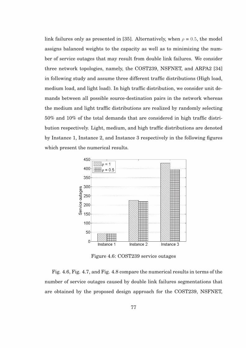
link failures only as presented in [35]. Alternatively, when ρ = 0.5, the model

assigns balanced weights to the capacity as well as to minimizing the num-

ber of service outages that may result from double link failures. We consider

three network topologies, namely, the COST239, NSFNET, and ARPA2 [34]

in following study and assume three different traffic distributions (High load,

medium load, and light load). In high traffic distribution, we consider unit de-

mands between all possible source-destination pairs in the network whereas

the medium and light traffic distributions are realized by randomly selecting

50% and 10% of the total demands that are considered in high traffic distri-

bution respectively. Light, medium, and high traffic distributions are denoted

by Instance 1, Instance 2, and Instance 3 respectively in the following figures

which present the numerical results.

Figure 4.6: COST239 service outages

Fig. 4.6, Fig. 4.7, and Fig. 4.8 compare the numerical results in terms of the

number of service outages caused by double link failures segmentations that

are obtained by the proposed design approach for the COST239, NSFNET,

77

Figure 4.7: NSFNET service outages

and ARPA2 networks respectively. Each comparison consists of three traffic

distributions: Instance 1 for light, Instance 2 for medium, and Instance 3 for

high traffic scenarios.

The figures show that when ρ = 0.5, the number of outages resulting from

double link failures is reduced and the reduction becomes substantial for traf-

fic instance 3 (i.e., at high loads). For example, when ρ = 0.5, the design model

achieves a reduction of 13.3% in the number of service outages for NSFNET

network at the cost of only 6.9% increase in capacity deployment (Table 4.2)

by comparison to the values when ρ = 1. Clearly, a higher value of ρ yields

a more effective capacity allocation, which is obtained at the cost of having a

network that is more vulnurable to service outages in the presence of double

link failures and results lower service availability. Similar results are observed

for COST239 and ARPA2 (Fig. 4.7 and Fig. 4.8) where the number of service

outages is reduced by 8.1% and 3.3% respectively at the cost of 7.0% and 2.8%

(Table 4.2) increase in capacity deployment for NSFNET and ARPA2 networks

78

Figure 4.8: ARPA2 service outages

Table 4.2: Capacity trade-off between two approachesCOST239 NSFNET ARPA2

ρ = 1 ρ = 0.5 ρ = 1 ρ = 0.5 ρ = 1 ρ = 0.5

(unit capacity) (unit capacity) (unit capacity)Instance 1 34 36 68 76 179 188Instance 2 172 183 299 314 952 981Instance 3 310 332 589 630 1856 1908

respectively.

4.1.4 Further Observations

By further dissecting the above numerical results, we observe that the reason

some of the connections are vulnerable to a second failure is due to the lack

of provisioned capacity. For example in traffic instance 3 of previous section,

we identified that 22% - 32% of the total outages that may be caused by dou-

ble link failures are due to insufficient capacity in the network, after restoring

all connections affected by the first failure. In light of this observation, the

79

service outages in ERP can further be characterized into three categories: (i)

outages due to physical segmentations, (ii) outages due to logical segmenta-

tions, and (iii) outages due to lack of capacity. The first two categories have

been addressed by the proposed ILP model on Section 4.1.2 which minimizes

the number of outages caused by the logical segmentations while the physical

segmentations are referred as unavoidable. Now, we address the third cate-

gory of service outages and its possible remedy.

In an efficiently designed ERP mesh network, the spare capacity that is

reserved for protection switching is shared as much as possible between exist-

ing connections. When a link fails, all of the connections that are traversing

the link are disrupted. The network enters into a failure state and all of the

affected connections are restored via alternate available paths. At this point,

all of the connections in the network are operational; however some of these

connections, more precisely the connections that share spare capacity with the

affected connections of the first failure, are vulnerable to subsequent failure.

Thus, one needs to identify these connections which are vulnerable in the pres-

ence of multiple concurrent failures and provision capacity in the network in

a way to reduce the number of possible service outages caused by multiple

failures.

We represent the network state (working/failure) by a binary link-state vec-

tor Sk [36], [28], such that Sk = {Sk,� = 0 for blocked links; 1 otherwise. ∀� ∈

L}. A link � can be referred to as blocked if either it is selected as an RPL in

working state or it is affected by a failure. Then, the set of K different link

state vectors corresponds to all possible single-link failure scenarios. Each Sk

represents a tree of the network which uniquely determines the forwarding

80

paths and corresponding link loads. The load of link � is the number of con-

nections passing through it and is denoted by λ�(Sk) which is interchangeably

referred to as the required capacity of link �. Let us denote the link capacity

vector by C�′

� which is an integer set and specifies the number of connections

that are traversing link �′ in working state and are provisioned to traverse link

� in case of failure on link �′ . Then C�

′� ≥ λ�′ (Sk), ∀�

′ ∈ L. Thus, the amount

of capacity which needs to be reserved for protection switching on link � is

C∗� = max

∀�′C�

′� . However, when a failure occurs and the protection switching is

activated, some of the spare capacity on link � may be used. In such event,

C∗� should be updated according to the current network state. One may find

that C� ≤ C∗� , where C� is the amount of spare capacity still available on link �

after first failure occurred. C� < C∗� also represents that some connections may

contend for the spare capacity on link � upon next failure and may become vul-

nerable. Such connections are referred to as Vulnerable Connections while the

rest of the connections which have C� ≥ C∗� on all of the links of their working

and restoration path are referred to as Protected Connections. To illustrate

better the service outages due to lack of capacity, we present an example as

follows.

Fig. 4.9(a) presents an ERP network with the logical hierarchy of two inter-

connected rings and the corresponding RPL positions. Two services (one unit

each) are requested from node B to node F (c1) and from node H to node F

(c2) which are routed through B − C − F and H − I − F respectively in work-

ing (Idle) state. Fig. 4.9(b) shows the capacity allocations (C∗� ) on each link

(presented besides each link). Let us assume that the first failure occurred on

link C − F and the affected connection c1 is restored through alternate path

B−A−D−E−F (Fig. 4.9(c)). Now, we update the value of C∗� according to the

81

(a)

(b) (c)

A B C

D E F

G H I

RPL

RPL

Major Ring

Sub-ring

X

X

0 0

A B C

D E F

G H I

RPL

RPL

Major Ring

Sub-ring

1 1

11

1 1

1 1

1 1

A B C

D E F

G H I

RPL

RPL

Major Ring

Sub-ring

1st

failure

2nd

failure

Figure 4.9: Service outages due to inadequate capacity

82

current network state and find that C∗�DE

= 1 and C∗�EF

= 1, however C�DE= 0

and C�EF= 0, i.e., no spare capacity is available on links D−E and E−F after

link C − F fails and the connection c2 becomes vulnerable to next failure. Let

us now assume that another failure occurs on link F − I before the repair of

link C − F . Then c2 cannot be restored and it experiences service outage due

to lack of capacity on links D − E and E − F .

Suggested Remedy

Contention for capacity among vulnerable connections can be resolved by re-

serving more spare capacity on the links that are shared by these contending

connections. We develop a procedure to estimate the amount of additional

capacity requirement on contention links. The overall requirement of spare

capacity in the network is recomputed in the subroutine such that all of the

service outages due to lack of capacity are eliminated while the amount of

spare capacity is minimized.

The developed routine operates on the optimal configuration found by the

ILP model of Section 4.1.2, i.e., we assume the logical hierarchy of the inter-

connected rings and their corresponding RPLs are given to the routine. The

function iterates over all single-link failure situations as described in the pro-

cedure ESTIMATE-SPARE-CAPACITY. The average running time of the rou-

tine is in the order of O(LC+L2) where L and C are the number of bidirectional

links and the number of connections respectively. We denote the affected link

by �′ . We identify the set of affected connections, restore them and update C∗

�

for each link � ∈ L. Then we build the set of link state vectors S of K dif-

ferent link states. Each item Sk in the set S represents a double link failure

scenario by blocking the first link �′ and any other link �

′′: �

′′ ∈ L and �′′ �= �

′ .

83

We identify the set of vulnerable connections for each element Sk and com-

pute the required additional capacity C�′,�′′

�,k on each contending link such that

C�′,�′′

�,k = C∗� − C�. Then we evaluate the additional spare capacity which needs

to be provisioned on link � by C�′,�′′

� = max∀k

C�′,�′′

�,k and update the value of C∗� by

C∗� + C�

′,�′′

� . Note that some of the elements Sk in S may represent physical or

ESTIMATE-SPARE-CAPACITY 4.1 Capacity estimation1: Input: Network topology, traffic matrix, logical design;2: Output: Additional capacity per link to be provisioned;3: for all failure on link �

′ ∈ L do4: Identify the set of affected connections Ca;5: Make necessary changes to the network topology (i.e., blocking failed link port,

unblocking corresponding RPL);6: for all c ∈ Ca do7: Restore the affected connection c;8: end for9: for all � ∈ L do

10: Update C∗� and C�;

11: end for12: Build the link state vector S of K items: each Sk represents double (�′ , �′′) fail-

ures;13: Compute C�

′,�′′

�,k such as C�′,�′′

�,k = C∗� − C�;

14: for all � ∈ L do15: Compute C�

′,�′′

� = max∀k

C�′,�′′

�,k ;

16: end for17: return C�

′,�′′

� ;18: end for

logical segmentations and hence, some of the connections may suffer service

outages due to this. We ignore to restore such connections in the subroutine.

Dual-failure restorability

Finally we extend our study to analyze the impact of our network design ap-

proaches on the level of network restorability. The double link failures restora-

bility R�′,�′′

2 of a given pair of links (�′ , �′′), as defined in [36], is the fraction of

the total failed connections traversing through links �′ and �

′′ in working state

84

that can be restored in the case of concurrent dual failures on links �′ and �

′′ .

Let us denote the number of non restorable connections in the case of failure

on links �′ and �

′′ by F�′ ,�′′ and the connections that traverse link �′ and �

′′ in

working state by W c�′ and W c

�′′ respectively. Then, the restorability R�′,�′′

2 can be

defined as: R�′,�′′

2 = 1 -F�′,�′′

W c

�′+W c

�′′

. The network-wide restorability is denoted by

R2 which is defined as the average of over all ordered (�′ , �′′) double link fail-

ures combinations [36]. Then R2 = 1 -

∑

∀(�′ ,�′′ ):�′ �=�′′F�′,�′′

∑

∀(�′ ,�′′ ):�′ �=�′′(W c

�′+W c

�′′ )

. The above presented

subroutine is used to compute the network-wide restorability as well and the

numerical results are presented as follows.

Numerical Results II

Figure 4.10: COST239 service outages

In this section, we analyze the additional capacity requirement estimated

85

by the suggested remedy to eliminate the service outages due to the lack of ca-

pacity and the impact on the service outages. We compare the capacity-outages

trade-off with the results that are presented in Section 3.5. The numerical re-

sults compare three design approaches: the first two approaches are different

variants of the ILP model (ρ = 1 and ρ = 0.5 without modifications of Section

4.1.4) and the third approach (ρ = 0.5 with modifications of Section 4.1.4) es-

timates the additional capacity required to completely protect all restorable

connections. We adopt the same traffic distributions as of numerical results

presented in Section 4.1.3.

Figure 4.11: NSFNET service outages

Figs. 4.10, 4.11, and 4.12 present the number of service outages in three

different network instances COST239, NSFNet, and ARPA2 respectively with

different traffic distributions and Table 4.3 shows the corresponding capacity

requirements. The figures show that our suggested remedy in the procedure

86

ESTIMATE-SPARE-CAPACITY can further reduce the number of service out-

ages in the networks. For example, in COST239 with high traffic load (In-

stance 3), 15.6% of additional capacity (Table 4.3) yields a 27.1% reduction in

service outages over the previous design method (ρ = 0.5). Similar results are

observed for NSFNet and ARPA2 networks where the number of service out-

ages are shown to be reduced by 32.7% and 21.9% in traffic instance 3 with

additional 17.9% and 16.5% capacity investment respectively.

Figure 4.12: ARPA2 service outages

Fig. 4.13 presents the network-wide double link failures restorability (R2)

that can be achieved by the three design approaches in three network in-

stances with high load (Instance 3). The figure shows that the network-wide

restorability is improved by the third approach for all three network instances

at the cost of additional capacity deployment. The first design approach (ρ = 1)

which was intended to achieve 100% restorability against any single-link fail-

ure can achieve 81% restorability against double link failures (R2) in NSFNet

87

Figure 4.13: Comparison of network-wide restorability

network with high traffic load (Instance 3) and R2 can be increased by 10%

with additional capacity investment as estimated by the third approach. Sim-

ilar trends are observed for COST239 and ARPA2 networks as well. A service

provider may be interested to estimate the amount of capacity need to be de-

ployed to achieve a targeted level of restorability.

4.2 Joint approach

Previous section addressed the problem of minimizing category-1 outages as

part of the network design; it turns out that such service outages strongly

depend on the particular RPL placement as well as the selection of the rings

hierarchy. Our study reveals that the number of category-2 service outages

which may occur under dual link failures is not negligible, as demonstrated

in Table 4.4. Table 4.4 depicts some representative results on the outages per

88

each category for COST239 network using the design approach of previous

section. Clearly, a sizeable fraction of category-2 outages may affect the net-

work and cannot be ignored in the design. This section addresses the problem

through a joint design approach where all outages resulting from concurrent

dual link failures are minimized while capacity is optimally allocated on the

links. We present a modified MILP formulation for the network design. The

numerical results show that the two-step method cannot guarantee the opti-

mality of the solution, whereas the proposed joint approach consistently yields

to finding the optimal solution.

4.2.1 Category - 2 Outages

Given a network which is designed to survive against any single link failure,

the provisioned capacity for its protection plan may be shared among demands

which do not belong to the same risk groups. Upon a failure, all affected con-

nections are restored through the reserved protection capacity; however, some

connections may become vulnerable to a subsequent failure, especially those

connections that share their protection plan with the connections affected by

the first failure. These “vulnerable” connections are either completely unpro-

tected for a second failure or may be in contention for resources with other

connections which may be affected by a second failure. Thus, a second fail-

ure may yield network outages. Had enough capacity been provisioned, these

outages may be mitigated. For example, let us assume that the network in

Fig. 4.14 is designed to protect the two given connections (as shown) against

any single link failure and the number on each link represents the allocated

capacity. Note that, both connections are sharing protection resources on links

D−E and E −F where only one (1) unit of capacity on each of the two links is

89

(a) (b) (c) (d) (e)

A B C

D E F

G H I

RPL

RPL

Major Ring

Sub-ring

1

1

1

11

1 1

1

2

2

X

X

Contention

A B C

D E F

G H I

RPL

RPL

Major Ring

Sub-ring X

X

1

1

1

11

1 1

1

2

2

A B C

D E F

G H I

RPL

RPL

Major Ring

Sub-ring

X

X

1

1

1

11

1 1

1

2

2

A B C

D E F

G H I

RPL

RPL

Major Ring

Sub-ring

XX1

1

1

11

1 1

1

2

2

A B C

D E F

G H I

RPL

RPL

Major Ring

Sub-ring

1

1

1

11

1 1

1

2

2

Figure 4.14: Category-1 and category-2 outages

needed to protect the given connections. However, in case of dual concurrent

links failure scenario as presented in Fig. 4.14(d), where the two connections

are affected together, both demands contend for the shared capacity. Assuming

that the first failure occurs on link C − F , then connection B − I is restored

by using the shared resources causing the other connection (H − I) to become

unprotected against a subsequent failure. If the subsequent failure occurs on

link H − I, the connection (H − I) will suffer service outage.

4.2.2 Illustrative example

Given the sequential nature of the design method of previous section, the over-

all solution may not be globally optimal as demonstrated in following illustra-

tive example. Fig. 4.15 depicts a mesh network composed of three rings R1,

R2, and R3 and three connection requests C − H, B − G, and E − C. Fig.

4.15(a) presents a capacity allocation solution (as well as RPL placement and

hierarchy selection) obtained from the optimization model of previous section

whose objective is to jointly minimize capacity and category-1 outages. The

RPL placements are located and the logical ring hierarchies of the network

are presented by the dotted lines. The solid lines represent the routing of the

90

connection requests in working state and the numbers besides each link rep-

resents the capacity allocation on the links. The given solution requires in

total 22 units of capacity to survive against any single link failure and there

will be 29 possible instances of service outages (18 category-1 outages and

11 category-2 outages) due to dual-link failure scenarios. After exhaustively

enumerating all possible dual-link failure scenarios, we found that two links

(D − I, I − H) require additional capacity of 3 units on each link to eliminate

category-2 service outages. For example, let us consider a dual link failure sce-

nario where links D−E and A−F fail concurrently. Upon failure, the rings R1

and R3 unblock their RPLs and all three source-destination pairs remain con-

nected. Connections C −H, B −G, and E −C are intended to reroute through

C − D − I − H, B − C − D − I − H − G, and E − H − I − D − C respectively.

However, links D − I and H − I do not have the required protection capacity

to carry the rerouted demands. Indeed, three (3) units of additional capacity

on each link D − I and H − I could provide the necessary protection against

the given dual-link failure scenario. Hence, overall 28 (22+6) units of capac-

ity are required by the two steps solution to eliminate category-2 outages and

then, there will be 18 possible instances of category-1 outages. In contrary, Fig.

4.15(b) illustrates an alternate solution, which can be obtained by a joint so-

lution approach. The solution presented in Fig. 4.15(b) shows different logical

hierarchy of the rings as well as different RPL positions of the previous solu-

tion. This solution requires 27 units of overall capacity to eliminate category-2

outages while the category-1 outages remain 18 which is equal to the previous

solution. The illustrative example clearly demonstrates the necessity to solve

the two problems jointly to overcome the limitation of previous work.

91

R1

RP

L

RPL

A

B

C D

E

F G

H

I

RP

L

R2

R3

(b)

3

3 3

1

2 3

2

3 3

1

3

R1

RPL

RPL

A

B

C D

E

F G

H

IRPL

R2

R3

(a)

3

3 3

2

2 3

2

3 0

1

0

Figure 4.15: Illustrative example


Analysis

The previous section clearly highlights the need to jointly address category-1

and category-2 outages within the network design. As opposed to the sequen-

tial method, now we lay out our methodology for addressing this joint design

problem. We demonstrate that both outage categories can be combinedly re-

duced by maximizing the number of connections that could be established, i.e.,

maximizing network flows, under any dual link failure scenarios. In this sec-

tion, we present our analysis to show that maximizing network flows implies

minimizing segmentations (category-1) and that a flow conservation constraint

for protection switching, as illustrated next, ensures that enough capacity is

allocated on each link to eliminate category-2 service outages.

We denote a network topology by a graph G(V ,L), where V is the set of

vertices and L is the set of links, indexed by v and � respectively. The set of

all possible ring hierarchies and the RPL placements are denoted by H and

Z and indexed by h and Z respectively. The set of the simple rings in G is

denoted by R and is indexed by r. A simple ring is composed of a set of links

that form a physical ring/cycle with no straddling links. For example, in Fig.

92

4.14(a), links {AB,BC,CF, FE,ED, and DA} forms a simple ring whereas

links {AB,BC,CF, FI, IH,HG,GD, and DA} also form a physical ring but we

do not refer to it as simple ring since there are two straddling links (DE,EF ).

The traffic demand set is denoted by T . Each element of this set, t, defines a

unit demand from source st to destination dt where st, dt ∈ V. We denote F

as the set of all possible dual failure scenarios where each element of this set,

f , represents a dual failure of any links � and �′, where �, �′ ∈ L.

Definition 1. A configuration c(G, h, Z) is an ERP network G with a given

logical hierarchy h among interconnected rings and the set of RPLs Z of the

rings. The set of all possible configurations of a given ERP network is denoted

by C.

Definition 2. A feasible flow for a demand t in a configuration c experiencing

an instance of dual-link failure f is denoted by xtf,c such that:

(a) For every vertex j : j ∈ V − {st, dt},∑i∈V

xtf,c(i, j) =

∑k∈V

xtf,c(j, k) where xt

f,c(i, j)

is the amount of flow on a link (i, j) between two adjacent nodes i and j.

(b)∑i∈V

xtf,c(st, i) =

∑i∈V

xtf,c(i, dt) ≥ 0.

The amount of flow for a demand t in configuration c is∑f∈F

xtf,c.

Definition 3. A segmentation in a network affecting a demand t is a partition

of V into at least two disjoint sets V ′ and V ′′ such that st ∈ V ′ and dt ∈ V ′′ caused

by an instance of concurrent dual-link failure f .

Definition 4. Let P(t, r) be a segment of a path used by a demand t which

contains one or more edges of ring r and P(t, r) be the other segment of r. Let

|P(t, r)| and |P(t, r)| be the number of links in these segments respectively. Then,

the number of service outages that the demand t may possibly suffer from seg-

mentations resulting from dual link failures in a given configuration c can be

93

defined as otc =∑r∈R

{|P(t, r)| × |P(t, r)|}.

Definition 5. The net flow of a given configuration c is

X(c) =∑f∈F

∑t∈T

xtf,c

and the net service outages of a given configuration c is

O(c) =∑t∈T

otc

Lemma 1. The number of service outages otc that a demand t will possibly suffer

from segmentations is known for a given ERP configuration c and is given by

Definition 4.

Proof. By definition, a given ERP configuration c always forms a logical tree

and hence, the routing of any given demand t is unique. Once the routing

is determined, P(t, r) and P(t, r) are trivially found and thus the otc can be

determined.

Lemma 2. Let otc and otc′ be the number of service outages that demand t may

suffer from segmentations resulting from dual link failures in configurations c

and c′ respectively. If otc > otc′ then∑f∈F

xtf,c <

∑f∈F

xtf,c′ .

Proof. The set of all possible dual failure scenarios in a given network topology

is defined by F . The number of elements in F , |F|, depends on the number of

links in the network and can be determined by N(N−1)2

where N is the number

of links. The number of service outages that a demand t may suffer in config-

uration c, otc, can be determined by Definition 4, which depends on the number

of links of each ring traversed by the demand t. Since, one of the links of each

ring must be configured as the RPL and the demand t cannot be routed through

the RPL, it is evident that otc < |F|. Hence, there exist some instances of dual

94

failures which do not cause service outages for demand t in configuration c.

Let F ′c,t and F ′′

c,t be the subsets of dual failures which cause and, respectively,

do not cause service outages for demand t in configuration c, i.e., F ′c,t, F ′′

c,t ⊆

F . Let f ′c,t and f ′′

c,t be the number of elements of these subsets respectively, i.e.,

f ′c,t = |F ′

c,t| and f ′′c,t = |F ′′

c,t|.

Now, from Definition 2, the amount of flow for a demand t in configuration c

can be expressed as ∑f∈F

xtf,c =

∑f∈F ′

c,t

xtf,c +

∑f∈F ′′

c,t

xtf,c

If a dual failure scenario f causes service outage for demand t in configuration

c, then there is no feasible flow for t in that particular dual failure scenario and

thus xtf,c = 0. Hence,

∑f∈F ′

c,t

xtf,c does not contribute in determining the amount

of flow for demand t. So, ∑f∈F

xtf,c =

∑f∈F ′′

c,t

xtf,c

Similarly, since the dual failure instances of F ′′c,t do not cause service outages

for demand t in configuration c, f ′′c,t has no contribution in determining otc.

Hence, if otc > otc′ for any configurations c and c′, we can say that f ′c,t > f ′

c′,t

and consequently f ′′c,t < f ′′

c′,t.

Since we assume unit demands, we conclude that if otc > otc′ ,∑

f∈F ′′c,t

xtf,c <

∑f∈F ′′

c′,t

xtf,c′ .

and thus, ∑f∈F

xtf,c <

∑f∈F

xtf,c′

Lemma 3. Let X(c) be the net flow of configuration c. If O(c) ≤ O(c′) then

X(c) ≥ X(c′).

Proof. From Lemma 2, we can say that if otc ≤ otc′ then∑f∈F

xtf,c ≥

∑f∈F

xtf,c′ for any

95

demand t in configuration c. Thus, accumulating over a given set of demands

T , we can state that if∑t∈T

otc ≤∑t∈T

otc′ then∑f∈F

∑t∈T

xtf,c ≥

∑f∈F

∑t∈T

xtf,c′ . However,

from Definition 5,∑t∈T

otc is equivalent to O(c) and∑f∈F

∑t∈T

xtf,c is equivalent to

X(c). By replacing these equivalent terminologies, we can conclude that if

O(c) ≤ O(c′) then X(c) ≥ X(c′).

Theorem 1. Let O(c) be the number of service outages resulting from segmenta-

tions in a given configuration c such that c = argminc∈C

O(c), then X(c) ≥ X(c′) ∀c′ ∈

C − {c}.

Proof. Let us assume that there is at least one configuration such that the

net flow in that configuration is greater than X(c), i.e., ∃c′ : X(c′) > X(c). In

such case, according to Lemma 3, the number of service outages resulting from

segmentations in configuration c′ must be smaller that O(c), i.e., O(c′) < O(c).

However, given that O(c) is the minimum outages among any configuration in

the network, we can conclude that O(c′) ≮ O(c). Hence, our assumption is a

contradiction, i.e., �c′ : X(c′) > X(c) and X(c) ≥ X(c′) ∀c′ ∈ C − {c}.

The above analysis clearly shows that in order to minimize outages result-

ing from dual concurrent failures, one could simply resort to maximizing net-

work flows, given all possible dual link failures. This design will be elaborated

in the next section.

ILP Formulation

We present our formulation for the joint optimal ERP design and capacity al-

location problem. We consider Ethernet transport networks with bidirectional

links where the capacity of each link is shared by the traffic in both direc-

tions. However, the network is presented by a graph G with directed arcs. The

96

required capacity of a link is determined by the amount of traffic traversing

through both of the corresponding arcs. A bidirectional link of the network is

denoted by � and the set of links is denoted by L. The corresponding directed

arcs of link � are denoted by �ij and �ji where i, j are two adjacent nodes and

i, j ∈ V and the set of directed arcs is denoted by E . The variables that are

used to determine the ERP design and the capacity of the links are indexed by

� while the variables that are used to determine the routing of the demands

are indexed by directed arcs �ij or �ji. We assume the set of simple rings R

is given. Note that, our design method allows some rings of R to be pruned

out. Some of the given simple rings may not need to be part of the logical

ERP instance since none of their links are traversed by any of the demands

in either working or protection state. A ring r is to be selected if and only if

some demands absolutely require one or more of its links to be routed either

in working or protection state. Capacity is provisioned only on the links of se-

lected rings. According to the ITU-T recommendation G.8032, if more than one

link are physically common to two rings, all of the common links must belong

to only one of the logical rings. For example, in Fig. 4.14(a), links DE and EF

are physically common to two simple rings. However, both of them must be-

long to either the upper ring or to the lower ring. It is restricted to design

an ERP instance such that link DE belongs to one logical ring and link EF

belongs to another logical ring. In this particular example, both links belong

to the upper physical ring and form a logical “Major ring”. We further assume

that the demands in T are unit-capacity demands. We define F as a set of

failure scenarios (F = {F (�, �′) : �, �′ ∈ L}) such that each element of this set

consists of a group of link(s) which for instance share the similar risk of failure

or potentially could fail concurrently. The probability of concurrent failures on

97

the links in the same group is considerably high because of common resource

sharing (e.g., sharing fiber, common routers, etc.). We define the following pa-

rameters, sets, and variables that are used in the formulation.

• Parameters and sets: α�r equal to 1 if link � belongs to ring r, 0 otherwise.

Lr is the set of links spanned by ring r ∈ R. St, Dt are the source and

destination of demand d, respectively.

• Variables: The variables are categorized into two classes based on their

functions. One class (class-1) is used to design ring hierarchies and RPL

placements whereas the other class (class-2) of variables is used in ca-

pacity planning and optimization.

Class-1 variables are similar to those are used in Section 3.4. We use the

following variables as class-2

• wt�ij

is used to determine the routing of the demands as well as the re-

quired capacity on the links in working state. wt�ij

: equal to 1 if demand

t is routed through arc �ij in working state, 0 otherwise.

• w�ij ,t

F(k) is a set of variables that is used to determine the routing as well as

capacity provisioning in protection state. w�ij ,t

F(k) : equals to 1 if demand t

is routed through arc �ij in case of k-th failure scenario of F , 0 otherwise.

• ψt� determines the required capacity on link � for demand t in working

state.

• ψ�,tF(k) determines the required capacity on link � for demand t in a failure

scenario F(k).

• ψ� determines the capacity needed to be provisioned on link �.

98

Similar to the variables, the constraints are categorized into two classes.

We reuse the set of constraints 3.1 to 3.6 for the design of ERP architecture.

The capacity planning constraints are defined as follows :

• In working state :

∑∀j:�ij∈E

wt�ij

−∑

∀j:�ji∈Ewt

�ji=

⎧⎪⎪⎪⎪⎪⎪⎪⎨⎪⎪⎪⎪⎪⎪⎪⎩

1 if i = St

− 1 if i = Dt

0 Otherwise

t ∈ T (4.7)

wt�ij

≤ 1−∑r∈R

η�r t ∈ T , � ∈ L (4.8)

wt�ij

≤∑r∈R

y�r t ∈ T , � ∈ L (4.9)

Constraint (4.7) is the flow conservation of each demand t ∈ T in working

state. Constraint (4.8) states that the arcs �ij and �ji can be used to carry

traffic in working state only if their corresponding link � is not the RPL of any

ring. Similarly, constraint (4.9) ensures that a demand t can use the arcs �ij

and �ji only if � belongs to a ring. Similar to the constraints (4.8) and (4.9), two

additional constraints are to be added for other directed arcs of �.

• In failure/protection state :

99

∑∀j:�ij∈E

w�ij ,t

F(k) −∑

∀j:�ji∈Ew

�ji,t

F(k) =

⎧⎪⎪⎪⎪⎪⎪⎪⎨⎪⎪⎪⎪⎪⎪⎪⎩

≤ 1 if i = St

≥ −1 if i = Dt

= 0 Otherwise

t ∈ T ,F(k) ∈ F

(4.10)

w�ij ,t

F(k) ≤ |F(k)|+ 1−∑

�′∈F(k)�′∈Lr

y�′r −

∑r′:r′∈R−r

η�r′ t ∈ T , � ∈ L, r ∈ R,F(k) ∈ F

(4.11)

w�ij ,t

F(k) ≤∑r∈R

α�rxr t ∈ T , � ∈ L (4.12)

w�ij ,t

F(k) = 0 � ∈ F(k), t ∈ T ,F(k) ∈ F (4.13)

ψt� ≥ wt

�ij+ wt

�ji� ∈ L, �ij, �ji ∈ E , t ∈ T (4.14)

ψ�,tF(k) ≥ w

�ij ,t

F(k) + w�ji,t

F(k) � ∈ L, �ij, �ji ∈ E , t ∈ T ,F(k) ∈ F (4.15)

ψ� ≥ max(∑t∈T

ψt�, max

∀F(k)

∑t∈T

ψ�,tF(k)) � ∈ L (4.16)

100

Constraint (4.10) is the flow conservation in the protection state for each de-

mand t ∈ T and for each failure scenario in F . Note that, we relax the conven-

tional flow conservation approach in constraint (4.10). The conventional flow

conservation ensures the flows to be routed from their sources to destinations.

However, routing of all demands in ERP protection state might not be feasible,

especially under dual-link failure scenarios that may cause physical/logical

segmentations. The relaxation of the flow conservation in constraint (4.10) al-

lows some demands not to be routed when there is no route available between

source and destination due to the segmentations and this circumvents the in-

feasibility of the model. Constraint (4.11) states that, the affected demands

by a failure scenario F(k) cannot be restored through arcs �ij and �ji, if their

corresponding bidirectional link � is the RPL of a ring other than the ring(s)

containing the failed link(s). For instance, let us assume that link A − B and

F −G fail concurrently in Fig. 4.15(b). The failed links belong to rings R1 and

R2 respectively. Upon a failure, both rings R1 and R2 unblock their RPLs C−D

and G−H respectively and the affected demands can be restored through the

corresponding arcs of those RPLs. However, the RPL H − I of ring R3 will

not be unblocked and thus, the affected demands cannot be restored through

the link H − I. Constraint (4.12) affirms that a link � is used to provide pro-

tection only if it belongs to a selected ring. Constraint (4.13) ensures that a

link cannot protect itself. Similar to the constraints (4.11), (4.12) and (4.13),

three additional constraints are to be added for other directed arcs of �. Con-

straints (4.14) and (4.15) are used for determining the capacity of the links by

transforming the traffic load of their corresponding arcs. Constraint (4.16) as-

sures that enough capacity is reserved on each link to carry demands in both

working and protection states.

101

The objective of the optimization problem is composed of two components.

The first component is to minimize the overall network capacity, to be pro-

visioned to withstand any single/dual link failures. The second component

is to maximize the overall outgoing flows from all given sources under any

single/dual-link failure scenarios. A parameter ρ is used as a “rewarding fac-

tor” for each successful restoration of the flows. The optimization solver may

need to explore alternate protection routes to restore affected demands and

may also require additional capacity to be provisioned. The rewarding fac-

tor ρ determines the amount to be rewarded over provisioned capacity for any

successful restoration. In other words, ρ provides the flexibility to network

designers to prioritize either increasing recoverable demands or reducing the

amount of capacity to be provisioned. The objective function is expressed as:

min

⎧⎨⎩∑

�∈Lψ� − ρ×

∑t∈T

∑∀F(k)

∑∀j:�ij∈E,i=St

w�ij ,t

F(k)

⎫⎬⎭

4.2.4 Numerical results

In this section, we evaluate the performance of our joint design method in

terms of minimal capacity requirement and total number of outages that the

network will suffer from following any concurrent dual-link failures. We note

here that the best design is indeed to provision minimal capacity in a net-

work that will only suffer a minimal number of service outages following any

dual failures. Most often though these are two contradicting objectives, as will

be shortly illustrated. We start by first presenting an evaluation of one ERP

design for optimal capacity allocation for protecting against only single link

failures (Previous work-1) [35]. We also present results for the ERP design

approach of previous section (Previous work-2). Both designs will be compared

102

with the joint design presented earlier in this paper. The objective of this

study is to illustrate the trade-offs between capacity provisioning and services

outages (following concurrent dual failures) experienced in the network. We

consider four traffic instances for this study (instances 1, 2, 3 and 4 consisting

of 30, 50, 70 and 100 demands respectively, randomly selected) and we use

the COST239 (11 nodes and 15 edges) for our evaluation and our results are

averaged over multiple runs. Our proposed model (Current work) is evaluated

with two different reward factors (ρ = 1 and 4). The numerical results are pre-

sented in Figure 4.16 which shows the overall allocated capacity (in terms of

unit demands) and the number of outages that result from all possible dual-

link failures. First, the figure shows that ignoring outages due to dual failures

(Previous work-1) yields to truly minimal capacity allocation in the network;

however, the price for this is the higher number of service outages caused by

dual failures, which yields to a lower service availability provided by the net-

work. Now considering minimizing category-1 outages (i.e., Previous work-2)

as part of the design will surely increase the service availability (notice the

reduction in the number of outages the network experiences) but indeed the

operator must invest more capacity in the network. Our proposed method (cur-

rent work) further reduces the service outages, in comparison with the other

two methods, since it jointly considers both outage categories in the design.

The figure shows the trade-off the reward factor plays; a high reward factor

suggests that more emphasis should be put on achieving higher service avail-

ability (minimizing outages by maximizing the flow of traffic in the network

under dual-link failure scenarios) and thus more capacity deployment in the

network while a smaller value of ρ puts more emphasis on minimizing capac-

ity and less so on service availability, therefore the higher number of outages

103

Figure 4.16: Performance Comparison with prior works using COST239 net-work

(the figure shows that outages are reduced by up to 37% over Previous work-1

and by up to 29% over Previous work-2 and that the additional investment in

network is 25% and 15% respectively). This study indeed shows the strong

relation between the allocated capacity and service availability; it also shows

that our proposed model gives network operators a choice to put more empha-

sis on either one, by properly adjusting the reward factor.

Next, we present a comparative study of our proposed joint design approach

with two other methods; namely, in the first one, the RPL placement and ring

hierarchy among interconnected rings are selected randomly (strategy-1), but

capacity is allocated to minimize dual link failure outages, and in the second

(strategy-2), the two step method is used. Our proposed method is referred to

as (strategy-3). We use four traffic instances for our evaluation, depicting light

to heavy loads (30, 50, 70, and 100 unit demands respectively whose sources

104

Instance 1 Instance 2 Instance 3 Instance 40

200

400

600

800

1000

Uni

t cap

acity

/un

it se

rvic

e ou

tage

s

Strategy−1Strategy−2Strategy−3Service outages

Figure 4.17: Comparison between different design strategies using Randomnetwork

and destinations are randomly generated); results are averaged over multi-

ple runs. Two networks are considered in our evaluation, a random network

with 9 nodes and 11 bidirectional edges (the topology presented in Fig. 4.15)

and COST239. The metrics of comparison are the allocated capacity and the

number outages following dual failures.

Fig. 4.17 and Fig. 4.18 present the numerical results from our evaluation

using the two networks. For both figures, the results for strategy 3 are ob-

tained by assuming a reward factor (ρ) of 4. The figures show that the random

strategy cannot guarantee the high service availability which may be required

by network operators, this is mainly due to the random placement of RPLs

and the selection of ring hierarchies (i.e., the design) that is done in a manner

which is oblivious to outages caused by network segmentations. The figures

show that this random design strategy results in network services which are

105

Figure 4.18: Comparison between different design strategies using COST239network

more vulnerable to dual failures and the number of service outages, in com-

parison with the other two strategies, is around 25% higher for some traffic

instances. In contrast, clearly, the other two design strategies achieve better

service availability, as depicted in the figures, than the random one which im-

plies the importance of properly selecting the RPL placement and hierarchy of

rings. Further, both strategies 2 and 3 aim at minimizing the number of out-

ages due to dual failures and hence achieve the same results; however, both

design methods are fundamentally different. Strategy 2 follows a sequential

approach and aims at minimizing 1) capacity allocated and category 1 outages

and then 2) allocate additional capacity to eliminate category 2 outages. On

the other hand, strategy 3 does the same but rather jointly, as explained ear-

lier, while provisioning less capacity in the network (8% less than strategy 2

and 3% less than strategy 1 for the random network). Similar conclusions can

106

1 1.5 2 2.5 3 3.5 4 4.5 5100

200

300

400

500

600

700

800

Reward factor (ρ)

Uni

t cap

acity

/un

it se

rvic

e ou

tage

s

Instance 1 (outages)Instance 2 (outages)Instance 3 (outages)Instance 4 (outages)Instance 1 (capacity)Instance 2 (capacity)Instance 3 (capacity)Instance 4 (capacity)

Figure 4.19: Comparison of capacity and service outages with varying rewardfactor (ρ) in COST239 network

be obtained from the COST239 network where the results are shown in Fig.

4.18.

Finally, we study the effect of varying the reward factor (ρ) on the perfor-

mance of our proposed joint design method. We note that a higher value of

ρ allows the model to favor maximizing the network flow subject to the set of

all dual failures (i.e., increase service availability) and a smaller value steers

the model to select designs which minimize the allocated capacity (recall, we

mentioned earlier, these two are opposing factors), with lesser emphasis on

outages. The results are presented in Fig. 4.19 for different traffic instances,

using the COST239 network. As shown (for example, at higher loads), smaller

ρ yields higher outages but smaller investment in capacity and higher values

of ρ results in smaller number of outages and slight increase in allocated ca-

pacity; there is a threshold value of the reward factor, beyond which no service

107

outages reduction can be seen. The threshold value of the reward factor varies

according to the network topology and the traffic pattern. In most of our exper-

iments, ρ = 3 is the threshold where service outages are minimized. Once this

threshold value is reached, increasing the reward cannot reduce the service

outages any further. Similar results are observed for the random network.

4.3 Chapter remark

In this chapter, we introduced and analyzed two categories of service outages

that the demands may suffer in an ERP-based mesh network under any dual

link failures. In Section 4.1, we developed an effective design approach for

ERP mesh networks which addresses the issue of category-1 service outages

and presented a routine to allocate additional capacity to eliminate category-

2 service outages. Section 4.2 presented an improved design approach that

jointly addresses both category of service outages. In Section 4.2, we presented

a theoretical analysis and formal proof which shows that maximizing network

flows subject to dual-link failures yields a network with high service avail-

ability and proposed an optimization model for solving this network design

problem. The optimization model provides network engineers with the design

flexibility to either minimize the provisioned capacity or minimize the service

outages or find a balance between capacity investment and service outages re-

sulting from dual link failures, by varying the value of a reward factor. Our

results indicate that substantial reduction (up to 37%) in service outages is

obtained over designs which are oblivious to dual link failures with little extra

capacity investment. Further, both design approaches of Sections 4.1 and 4.2

are compared. Our results indicate that similar network service availability is

achieved with less capacity deployment by later design model.

108

CO

ST23

9N

SFN

ET

AR

PA2

Inst

.1In

st.2

Inst

.3In

st.1

Inst

.2In

st.3

Inst

.1In

st.2

Inst

.3(u

nit

capa

city

)(u

nit

capa

city

)(u

nit

capa

city

)ρ=

134

172

310

6829

958

917

995

218

56ρ=

0.5

3618

333

276

314

630

188

981

1908

ρ=

0.5

wit

h45

218

384

9439

374

324

611

8122

24m

odifi

cati

onof

sec.

4.1.

4

Tabl

e4.

3:C

apac

ity

trad

e-of

fbet

wee

nth

ree

appr

oach

es

109

Table 4.4: Comparison of Category-1 and Category-2 service outagesCOST239 network

Number of demands Category-1 outages Category-2 outages

15 78 32

30 159 61

55 288 109

110

Chapter 5

Design of ERP: Traffic

Engineering

Previous chapters of this thesis have focused on minimizing the overall net-

work capacity requirement for a given set of traffic demand in ERP-based

mesh networks. The optimal capacity allocation (OCA) problem is resolved by

jointly selecting the ring hierarchy and determining the RPL placement using

optimization models for both single and dual link failure scenarios. However,

despite the importance of minimizing network cost through minimal capacity

deployment, network operators usually confront a different optimization chal-

lenge. Typically, a network operator may already have an existing network de-

ployed with finite link capacities and willing to implement ERP based protec-

tion mechanism. One of the most frequent design objectives is to maximize the

revenue through allowing as much traffic as possible in the network by proper

RPL placement and efficient selection of interconnected ring hierarchies. In

addition, network operators are interested to exploit another advantageous

feature of ERP which is the ability to implement multiple ERP instances over

a single underlying physical network. Implementing multiple ERP instances

111

could be beneficial for network operators in many different ways such as reduc-

ing end-to-end service latency, load balancing and so on which are discussed

in more detail in Section 5.2. However, it may increase the complexity of net-

work design. These network design issues and objectives are overlooked by the

previous ERP designs.

In this chapter, we address the above mentioned design objectives by jointly

determining the optimal RPL placement and selecting the ring hierarchies

such that the network flow is maximized for a given set of sessions (s-d pairs).

In the context of multiple ERP instances, it turns out that end-to-end service

latency is reduced as well while maximizing network flows comparing to the

one achieved by implementing single ERP instance. Section 5.1 presents the

MILP formulation of ERP design which considers a single ERP instances will

be implemented. The design strategy for multiple ERP instances is presented

in Section 5.2.

5.1 Traffic engineering over single ERP instance

The network flow can be maximized in a number of ways. One way is to formu-

late the problem as a maximum multi-commodity flow (MMCF) problem [37]

where the solution will maximize the flow, but may not fairly distribute the re-

sources among the sessions. Here, some flows may starve for resources while

some others (e.g. short hop flows) will be granted larger amount of band-

width. Similarly, links of some parts of the network may become saturated

keeping other parts underutilized. Another way to maximize network flows

is known as max-min approach which promises to fairly allocate bandwidth

among the sessions. Maximizing network flows has been extensively studied

during the last decade for different types of transport networks (e.g., WDM,

112

MPLS, wireless networks, etc.) [38, 39]. However, given the recency of the

Ethernet standard, this design remains unexplored in the context of ERP net-

works. Due to the unique operational principles, the design of ERP networks

require intense efforts. Nevertheless, previous works on flow maximization in

the context of other transport networks do not basically include backup pro-

visioning or design of a protection plan. In this work, we propose a novel

design approach with an efficient selection of RPL placement and ring hierar-

chy for any given deployed network implementing ERP. The design objective

is to maximize the network flows using the max-min approach and we develop

an ILP model to achieve this design objective. Our ILP model jointly provi-

sions backup/protection plan against any single link failure. To the best of our

knowledge, this is the first work addressing traffic engineering in the context

of ERP network design.

5.1.1 Problem Statement

Let G(V ,L) be a bidirectional graph with positive finite capacity c(�), ∀� ∈ L

and K be the number of sessions indexed by d1, d2, .., dk. Each of the sessions

is specified by the triplet di =< si, ti, γi > where si, ti denote the source and

destination of session i respectively and γi denotes its demand. Given the

capacity constraint on the links, satisfying all the incoming demands may not

be always possible. We define a rate vector δ whose elements δi denote the

rate assigned to the i-th session. A flow f si,ti is defined to be feasible if the

network can allocate enough bandwidth in both the working and protection

states to accommodate the allowable demand (δi × γi) of the session i. Note

that the network is provisioned to survive against any single link failure in

one ring. Therefore, the objective is to find the optimal RPL placements and

113

RP

L

(b)

R1

RP

L

A B

C

F

R2

5

5

3

5

5

5

5

E

D

R1

RPLA B

C

FRPL

R2

(a)

5

5

3

5

5

5

5E

D

Figure 5.1: Variations of granted flow in different RPL placement

ring hierarchies to maximize the minimum allowed rate δi of each session.

5.1.2 Illustrative Example

We present two illustrative examples to show the effect of two major ERP de-

sign components (RPL, ring hierarchy) on overall network flows. The first

example describes the impact of RPL placements whereas the second example

focuses on the effect of ring hierarchy.

Fig 5.1 shows a mesh network composed of two logical rings R1 and R2. Two

s-d pairs A − B and A − F are considered in this example each of which has

a demand of 3 units. The capacity of the links are presented by the numbers

placed beside each link. Fig. 5.1(a) shows an RPL placement on the links A−B

and E − F for rings R1 and R2 respectively. The hierarchy of the two rings are

shown by the dotted lines where R1 is the major ring and R2 is the sub-ring.

The connections between the s-d pairs are presented by the solid directed lines.

Note that, the capacity on link C − D does not allow us to grant more than

50% of the demands for each δi, i.e., 1.5 unit demand for each session. Fig.

5.1(b) shows an alternate RPL placement with the same ring hierarchy where

we can grant 83.3% of the requested demand, i.e., 2.5 unit demands for each

114

R1

RP

L

RPLA

B

C D

E

F G

H

IRPL

R2

R3

2

2 4

2

2 4

4

2 2

4

4

(b)

R1

RP

L

RPLA

B

C D

E

F G

H

IRPL

R2

R3

(a)

2

2 4

2

2 4

4

2 2

4

4

R1

RP

L

RPLA

B

C D

E

F G

H

IRPL

R2

R3

2

2 4

2

2 4

4

2 2

4

4

X

(d)

R1

RP

L

RPLA

B

C D

E

F G

H

IRPL

R2

R3

2

2 4

2

2 4

4

2 2

4

4

X

(c)

Figure 5.2: The impact of ring hierarchy on the amount of granted flow

session which increases the total amount of flow to 5 unit compared to 3 unit

of previous placement.

Similarly in Fig. 5.2, we show (by varying ring hierarchy for a fixed set

of RPL) that the selection of ring hierarchy affects the rate of the admissi-

ble flows. Fig. 5.2 shows a mesh network composed of three interconnected

logical rings R1, R2, and R3. We consider two sessions: d1 =< G,D, 3 > and

d2 =< I, F, 3 >. Fig. 5.2(a) and 5.2(b) show two different selections of ring

hierarchies, but the RPL placements are fixed. In Fig. 5.2(a), R1 is the ma-

jor ring and R2 is the upper ring w.r.t. the other sub-ring R3 whereas in Fig.

5.2(b), R3 is the major ring and R2 is the upper ring w.r.t the other sub-ring

R1. Ring hierarchies and link capacities are presented by the dotted lines and

the numbers beside each link respectively. The design of Fig. 5.2(a) limits the

allowable rate for each session by 33.3% and the overall net flow to 2 units.

Note that, the routing of the two sessions and the link capacities presented in

115

Fig. 5.2(a) show that the net flow/rate of each session can be further increased.

However, the definition of the feasible flow states that a protection plan has to

be provisioned for each admissible flow. Due to the lack of capacity on the links

of the provisioned protection paths (one such instance is shown in Fig. 5.2(c)),

the allowed rates δ1 and δ2 cannot be further increased for the ERP design of

Fig. 5.2(a). An alternate ring hierarchy is shown in Fig.5.2(b) where 2 units of

flow for each session can be provisioned (with 66.6% rate for each session) re-

sulting in overall net flow of 4 units, while ensuring the survivability against

any single link failure. Fig. 5.2(d) mimics the same failure scenario of Fig.

5.2(c) for the latter ERP design and shows that the capacity requirements on

the links traversed by protection paths are satisfied.


We consider a network (G) with bidirectional links, the set of simple rings1 in

G and the set of sessions D with demand vector γ are given. In addition to

the set of variables defined in Section 3.4, we define the following variables:

wdi� is used to determine the routing of the flows as well as the estimated flow

on the links in working state; it is equal to the amount of flow (δi × γi) of

session di which is routed through � in working state. w�,d�′ is used to determine

the routing as well as permissible flow in protection state: it is equal to the

amount of flow (δi × γi) of session di which is routed through � in case of failure

of �′.

The constraints of the MILP formulation are presented in different groups

based on their purpose of usage. The first set of constraints as defined in (3.1)

to (3.5) is reused in this model to design optimal ring hierarchies and RPL1A simple ring is a ring without any straddling links within its perimeter.

116

placements. Other constraints for flow routing and rate allocation are defined

as follows:

∑�∈v+

wdi� −

∑�∈v−

wdi� =

⎧⎪⎪⎪⎪⎪⎪⎪⎨⎪⎪⎪⎪⎪⎪⎪⎩

δi.γi if v = si

−δi.γi if v = ti

0 Otherwise

di ∈ D (5.1)

wdi� ≤ M(1−

∑r∈R

η�r) di ∈ D, � ∈ L (5.2)

wdi� ≤ δi × γi di ∈ D, � & �′ ∈ L (5.3)

wdi� ≤

∑r∈R

y�r di ∈ D, � ∈ L (5.4)

Constraint (5.1) is the flow conservation for the demands of a session di ∈ D in

working state. (5.2) states that a link � can be used to carry traffic in working

state only if it is not the RPL of any ring and (5.3) estimates the flow on � in

working state. M is a large integer. Similarly, (5.4) ensures that a session di

can use a link � only if � belongs to an activated ring.

∑�∈v+

w�,di�′ −

∑�∈v−

w�,di�′ =

⎧⎪⎪⎪⎪⎪⎪⎪⎨⎪⎪⎪⎪⎪⎪⎪⎩

δiγi if v = si

−δiγi if v = ti

0 Otherwise

di ∈ D (5.5)

w�,di�′ ≤ M(2− y�

′r −

∑r′∈R\r

η�r′)

di ∈ D, r ∈ R, � ∈ L (5.6)

117

w�,di�′ ≤ δi × γi di ∈ D, � & �′ ∈ L (5.7)

w�,di�′ = 0 � = �′, di ∈ D (5.8)

max(∑di∈D

wdi� , max

∀�′

∑di∈D

w�,di�′ ) ≤ c(�) � ∈ L (5.9)

Constraint (5.5) is the flow conservation in the protection state for sessions

di ∈ D in case link �′ fails. (5.6) states that the flows that are affected by a link

failure (�′) cannot be restored through link �, if � is the RPL of a ring other than

the ring containing �′. Constraint (5.7) estimates the flow on link � in case of

failure of link �′. (5.8) ensures that a link cannot protect itself. (5.9) limits the

admissible flow to the link capacity.

The objective of the optimization problem is to maximize the minimum δ

for any session which is expressed as:

max {min δiγi}


We evaluate the performance of our proposed design in terms of overall per-

missible network flows as well as fairness of resource allocation to incoming

sessions. We compare the performance of our ILP-based design method with

an arbitrary ERP design strategy (ARD) where the RPL placements and the

ring hierarchies are selected randomly. In both design methods, we use two

flow-maximization approaches. The first one is the max-min approach (ILP-

MM, ARD-MM) as presented in this paper. The other approach maximizes the

overall network flows with the objective of max∑K

i δiγi and referred to as ILP-

MF and ARD-MF. We present the numerical results for two well-known net-

work topologies: COST239 (11 nodes, 15 links) and NSF (14 nodes, 18 links)

118

10 20 30 40 500

20

40

60

80

No. of Sessions

Net

uni

t flo

w

ILP−MMILP−MFARD−MMARD−MF

Figure 5.3: Net flow in COST239 network

networks [34]. The link capacities are randomly chosen from the range of 10

- 50 units. The comparisons are shown for various network loads by varying

the number of sessions. The sources/destinations of the sessions are randomly

selected and the demand vector γ for the incoming sessions is uniformly dis-

tributed over the range of 1 - 5 units for each session. In all cases, the results

are averaged over multiple (5) runs.

Fig. 5.3 presents the permissible network flows in COST239 network as

we vary the traffic load. Clearly both ILP-MM and ILP-MF outperform the

arbitrary ERP design strategies (ARD cases). The overall network flow accom-

modated by ILP-MF is 38.5% greater than that of ARD-MF and is increased to

44.7% by ILP-MM than that of ARD-MM. The ILP-MF approach improves the

overall network flow by (2.4-4.5)% in some cases comparing to ILP-MM which

is somehow predictable, since ILP-MM rather focuses more on fair distribution

of flows among the sessions than increasing the overall network flows. Similar

results are observed for NSF network presented in Fig. 5.4 which shows that

119

20 40 60 800

20

40

60

80

100

120

140

No. of Session

Net

uni

t flo

w


Figure 5.4: Net flow in NSF network

ILP-MF increases the network flow up to 30%-38.4% than the ARD-MF.

10 20 30 40 500

0.5

1

1.5

No. of sessions

Jain

’s fa

irnes

s in

dex


Figure 5.5: Fairness in COST239 network

120

20 40 60 800

0.5

1

1.5

No. of Session

Jain

’s fa

irnes

s in

dex


Figure 5.6: Fairness in NSF network

Fig. 5.5 compares the fairness (Jain’s fairness index) in bandwidth allo-

cation achieved by different strategies in COST239 network. Again, the pro-

posed ILP-based design approaches (ILP-MM, ILP-MF) distribute the band-

width more fairly than ARD-MM and ARD-MF. Unlike to the net flow compari-

son, ILP-MM outperforms ILP-MF and achieves better fairness. In some cases,

ILP-MM achieves 27.7% and 48.8% better fairness in comparison to ILP-MF

and ARD-MF respectively. Similar results are observed for NSF network in

Fig. 5.6 where ILP-MM obtains significant improvement (0.8) in fairness over

ILP-MF (0.47) and ARD-MF (0.43) respectively especially with larger number

of sessions.

121

5.2 Traffic engineering over multiple ERP in-

stances

Network operators are expected to be naturally interested to implement mul-

tiple ERP instances over a single underlying physical ring since multiple ERP

instances can be utilized to reduce end-to-end service latency and to improve

resource utilization. This can be achieved without any increase in capital ex-

penditure (capEx) and with a little impact on operational expenses (opEx). The

effect on opEx includes increased complexity in network design and in ERP

configurations. Multiple ERP instances are managed and controlled by the use

of VLAN identifiers (VIDs). Customer traffic from one VID or a group of VIDs

are mapped to be protected by one of the ERP instances. The performances

of network services that are protected by ERP, e.g. end-to-end service latency

is directly related to such mapping. Hence, in addition to the typical ERP de-

sign issues (RPL placements and ring hierarchy selection), mapping customer

traffic to protecting ERP instance requires careful consideration, in order to

ensure optimized network performances, resulting in increased complexity in

network design. In this section, we study this combinatorially complex design

challenge of implementing multiple ERP instances in interconnected multi-

ring mesh networks and develop an optimization model which provides neces-

sary guideline to overcome this challenge.

5.2.1 Operation of multiple ERP instances

Since ERP is a logical entity, one can activate/implement multiple ERP in-

stances over a single underlying physical ring or interconnected rings. Each

ERP instance maintain its RPL, RPL owner node and RPL neighbor node. The

122

RPLs of different ring instances may be configured as different links or a single

link. Each ERP instance activate its own R-APS channel for failure notifica-

tion and protection switching procedures. The R-APS channel for different

ERP instances are differentiated by the use of different VIDs. Delivering and

protecting traffic channels by multiple ERP instances are also managed by

the use of VIDs. Traffic channels are either identified by separate VLAN or

grouped into different sets of VLANs. Each ERP instance is configured to pro-

tect a subset of those VLANs. When a failure is notified, each ERP instance

act independently based on the received control messages of its own R-APS

channel.

5.2.2 Design perspectives using multiple ERP instances

According to the ITU-T G.8032 recommendation, while implementing multi-

ple ERP instances, each ERP instance may select its own RPL independently.

One can take advantage of this feature to reduce the end-to-end service latency

compared to implementing single ERP instance. Implementing multiple ERP

instances can also be useful to avoid congestion in some parts of the network

and to ensure fair utilization of network resources. Multiple ERP instances

can be implemented without increasing capEx for network operators, though

it requires a VID to be assigned to each R-APS channel of each ERP instance.

Hence, a network operator might desire to implement as many ERP instances

as required. Virtually, there is no limit on the number of ERP instances that

could be implemented over a physical topology. However, it might not be ad-

vantageous to implement two or more ERP instances with the same link con-

figured as their RPLs. Thus, the suitable number of ERP instances could be

equal to the number of links where each link would be configured as the RPL

123

of one ERP instance. Besides, some other factors may limit the number of ERP

instances to be implemented. One of these factors is that Ethernet switches

may pose a limit on the number of ERP instances to be configured. Indeed,

given the recency of the ITU-T recommendation, only few vendors’ equipment

support the implementation of multiple ERP instances while limiting the max-

imum number of ERP instances to be implemented by two. However, the trend

is growing. The requirement of VID for each ERP instance also somehow limit

the implementable number of ERP instances. The number of VIDs that a ser-

vice provider can use is limited (around 4000) and service providers may wish

to use as many VIDs as possible to carry customer traffic. Hence, fewer num-

ber of VIDs would be reserved for implementing multiple ERP instances.

RPL

A

B

C D

E

F

(a) Physica ring

A

B

C D

E

F

(b) t1

A

B

C D

E

F

(c) t2

A

B

C D

E

F

(d) t3

A

B

C D

E

F

(e) t4

A

B

C D

E

F

(f) t5

A

B

C D

E

F

(g) t6

RPL

RPL

RPL

RPL

RPL

Figure 5.7: Logical ERP instances over a single physical ring

Once the number of multiple ERP instances to be implemented is chosen,

124

one needs to map the subset of VIDs that are carrying customer traffic to suit-

able ERP instances. This adds another dimension of complexity to the network

design consists of selection of RPL placements and the ring hierarchies. In the

context of multiple ERP instances, the selection of RPL placements represent

the selection of a subset of preferred ERP instances to be implemented among

the set of all possible ERP instances. The subset of preferred ERP instances

can be chosen based on the objective of network design. One of the important

design objectives for network operators could be reducing end-to-end service

latency. Such a network design should identify the best possible subset of ERP

instances, i.e., the RPL placements for each ERP instance and the hierarchy

among interconnected rings. However, one of our previous studies shows that

the selection of RPL placements and ring hierarchies play important role in

determining maximum admissible traffic flows in a network with fixed capac-

ity. Thus, certainly there is a trade-off between reducing end-to-end service

latency and allowable traffic flows while determining the subset of ERP in-

stances to be implemented. Next, we present an illustrative example which

visualizes this trade-off.

5.2.3 Problem Statement

Let G(V ,L) be a bidirectional graph with positive finite capacity c(�), ∀� ∈ L

and each link is assumed to have unit latency, i.e., the route with minimum

hop count represents the route with minimum latency. Let k be the number of

sessions indexed by d1, d2, .., dk. Each of the sessions is specified by the triplet

di =< si, ei, γi > where si, ei denote the source and destination of session i

respectively and γi denotes its demand. Given the capacity constraint on the

links, satisfying all the incoming demands may not be always possible. We

125

define a rate vector δ whose elements δi denote the rate allowed for the i-th

session. A flow f si,ei is defined to be feasible if the network can allocate enough

bandwidth in both the working and protection states to accommodate the al-

lowable demand (δi × γi) of the session i. Note that the network is provisioned

to survive against any single link failure in one ring. Therefore, the objec-

tive is to find the set of optimal virtual topologies, i.e., multiple ERP instances

with their RPL placements and ring hierarchies, in order to either minimize

the overall service latency or to maximize the minimum allowed rate δi of each

session or to strike a balance between both.

5.2.4 Mapping Problem

As mentioned earlier, the number of implementable ERP instances is limited

by either the number of reserved VIDs or by vendors’ specifications. Regard-

less of the source of the imposed limitation, a network operator must select a

subset of ERP instances to be implemented among all the possible instances in

order to satisfy the imposed constraint. The preference may vary according to

the network design objective. The selected ERP instances are then configured

to provide protection to a group of traffic flows differentiated by their VIDs.

We define the “mapping subproblem” as the mapping of a group of VLAN-IDs

(traffic flows) to one of the selected ERP instances which will be responsible

for providing protection to those mapped flows.

To illustrate, let us consider a simple ring topology with six links as shown

in Fig. 5.7(a). Six virtual topologies (t1, t2, . . . , t6) can be created over the given

physical ring by implementing six ERP instances where six different links

126

(a) arbitrary RPL selection(b) efficient RPL selection

in single ERP instance

(c) efficient RPL selection in multiple

ERP instances (working state)

R1

RPLA B

HRPL

R2

5

5

6

5

6

5G

C

5

5

3 3E DF

I

R1

RP

L

A B

H

RP

L

R2

5

5

6

5

6

5

C

5

5

3 3E DF

I

G

R1

RP

L

A B

H

RP

L

R2

5

5

6

5

6

5

C

5

5

3 3E DF

I

GRPL

R/

2

(d) efficient RPL selection in multiple

ERP instances (protection state)

R1

RP

L

A B

H

R2

5

5

6

5

6

5

C

5

5

3 3

I

X

F E D

G

R/

2

R/

2

Virtual topology 1

Virt

ual top

olog

y2

RPL

d2

d3

RP

LR

PL

R1

R2

d1

Figure 5.8: Illustrative example

would be configured as their RPLs as shown in Fig. 5.7(b) to Fig. 5.7(g) respec-

tively. The terminologies “ERP instance” and “virtual topology” are used in-

terchangeably hereafter. We further assume that the traffic flows are grouped

into three sessions (d1 =< C,F, 1 >, d2 =< A,F, 1 >, d3 =< A,C, 1 >) and at

most two virtual topologies are allowed to be implemented. Thus, one needs

to select two among the six possible virtual topologies and must map all three

sessions to any of the selected virtual topology. However, in order to select

127

two virtual topologies that are best suited according to the network design ob-

jective, all six virtual topologies require to be evaluated and compared based

on the measurement parameters. The number of comparisons can be repre-

sented by the sum of multinomial coefficient as∑

t1+t2+...+t6=3

(3

t1, t2, ... ,t6

)which is

equivalent to 63. In general, if there is m number of possible virtual topolo-

gies in a given physical network and k number of sessions to be mapped, the

total number of comparison would be∑

t1+t2+...+tm=k

(k

t1, t2, ... ,tm

)= mk. Hence, it

is computationally inefficient to exhaustively enumerate all possible combina-

tions to determine the best subset of virtual topologies in a larger network. In

the context of this particular example, let us assume that the virtual topolo-

gies t2 and t5 are selected and t2 is configured to protect sessions d1 and d3

while t5 is configured to protect d2 as shown in Fig. 5.7(c) and Fig. 5.7(f). Note

that, the RPL port is blocked based on VIDs in the implementation of multiple

ERP instances. Hence, when t2 is configured to protect the sessions d1 and d3,

the RPL of t2 will block the traffic on its port only from those VIDs that are

grouped to d1 and d3 while the traffic from VIDs that are associated with d2

will be allowed to pass through.

5.2.5 Illustrative example

Figure 5.8 presents an illustrative example to demonstrate the impact of ef-

ficient ERP design on network performance for both single and multiple ERP

instances implementations. Throughout this example, we consider a mesh net-

work composed of two interconnected rings and three sessions each of which

has a demand of 3 units, i.e., d1 =< A,B, 3 >, d2 =< A,H, 3 > and d3 =<

H,D, 3 >. The capacity of the links are presented by the numbers placed be-

side each link.

128

Figure 5.8(a) shows an arbitrary selection of RPLs with an implementation

of single ERP instance where R1 is the major ring and R2 is the sub ring. The

hierarchy of the two rings are shown by the dotted lines and the connections

between the s-d pairs are presented by the solid directed lines. Note that, the

capacity on links D−E and E−F do not allow us to grant more than 50% of the

demands for each δ1 and δ2 i.e., 1.5 unit demand for each session. Session d3 can

be granted 100% of its demand, however such amount of flow cannot be pro-

tected post failure of any of the two links H−I and I−D. Since we consider, in

our design approach, to guarantee 100% protection for allowed network flows,

d3 will also be granted 1.5 unit demand. On the other hand, service latency for

the given sessions are 4, 5 and 2 units respectively. A network operator may

however choose to design this network in a more efficient manner to achieve

the objective of minimizing overall service latency. The placements of RPLs

can be selected through an efficient network design as shown in Fig. 5.8(b)

resulting in overall service latency for the given sessions of 1, 3 and 4 units

respectively. However, the amount of flows to be granted remains 1.5 unit

demand for each session due to the capacity constraints on links D − E and

E − F .

So far, the benefits of multiple ERP instances are not exploited in this ex-

ample. Fig. 5.8(c) considers the same physical network topology and traffic of

Fig. 5.8(b) while the network is allowed to implement multiple ERP instances.

In addition to the ERP instance of Fig. 5.8(b) where R1 is the major ring and

R2 is the sub ring, another major ring is implemented over the lower physical

ring, referred to as R′2. The links H − I and G−H are configured as the RPLs

of R2 and R′2 respectively. The given session d3 is configured to be protected by

the ERP instance R′2. The ERP instance which is composed of the major ring

129

R1 and the sub ring R2 provides protection for the sessions d1 and d3. Figs.

5.8(c) and (d) show the working and protection states of the network with mul-

tiple ERP instances. Through the configuration of VIDs and mapping VID of

d2 to protecting ERP instance of R1 and R2, session d2 is allowed to be routed

through the RPL of R′2 in working state. In protection state of Fig. 5.8(d) where

link D− I fails, both R2 and R′2 unblock their RPLs. In this design, the service

latency for the sessions d1, d2 and d3 is reduced to 1, 3 and 2 units respec-

tively. In addition, the amount of flows to be granted for the given sessions is

increased to 3, 2.5 and 2.5 unit demands respectively resulting in an increase

of overall network flows comparing to previous designs implementing single

ERP instance.


We assume that the physical topology G(V ,L), where V is the set of nodes and

L is the set of links, and the capacity on each link C� are given. We define

the set of all possible hierarchies by H indexed by h and the set of all possible

virtual topologies in h by Th, indexed by t. We further assume that the set of

sessions D, indexed by di, with demand vector γ and the maximum number (Tp)

of virtual topology can be implemented are given. We use the parameter Lr as

a set containing the links spanned by physical ring r. We define the following

variables:

Zh : 1 if hierarchy h is chosen, 0 otherwise.

Kht : 1 if virtual topology t of hierarchy h is chosen, 0 otherwise.

ηh,tr,� : 1 if link � of ring r is RPL in virtual topology t of hierarchy h, 0 otherwise.

yhr,� : 1 if link � belongs to ring r in hierarchy h, 0 otherwise.

σh,tdi

: 1 if demand di is to be routed through virtual topology t of hierarchy h, 0

130

otherwise.

wh,t�,di

: amount of flow of session di traversed through link � in virtual topology

t of hierarchy h in working state.

P di� : 1 if session di traversed through link � in working state, 0 otherwise.

wh,t�,�′,di : amount of flow of session ditraversed through � in virtual topology t of

hierarchy h in case of link �′ fails and the network is in failure state.

The constraints of the MILP formulation are presented into different groups

based on their functionalities. The first set of constraints 5.10 to 5.15 is used

to build the logical relationship between the set of virtual topologies and the

RPL positions of each hierarchy.

∑h∈H

Zh = 1 (5.10)

∑t∈Th

kht ≤ Tp h ∈ H (5.11)

kht ≤ Zh h ∈ H, t ∈ Th (5.12)

∑�∈L

ηh,tr,� = 1 r ∈ R, t ∈ T , h ∈ H (5.13)

∑r∈R

yhr,� = 1 � ∈ L, h ∈ H (5.14)

yhr,� = yhr,�′ �, �′ ∈ Lr ∩ Lr′ , r, r′ ∈ R, h ∈ H (5.15)

Constraints (5.10) and (5.11) limit the number of hierarchy to be selected and

the number of implementable virtual topologies respectively. Constraint (5.12)

131

states that a hierarchy has to be selected to implement one of its virtual topolo-

gies. Constraint (5.13) ensures that a ring can have at most one RPL for each

virtual topology. In any given hierarchy, a link can belongs to only one ring

which is enforce by Constraint (5.14). Constraint (5.15) states that any set of

links that are shared by a pair of rings r and r′ must logically belong to only

one of those rings.

The other two sets of variables are defined for flow rate allocation and rout-

ing in both working ((5.16) to (5.23)) and protection ((5.24) to (5.28)) states as

follows:

∑t∈Th

∑�∈v+

wh,t�,di

−∑t∈Th

∑�∈v−

wh,t�,di

=

⎧⎪⎪⎪⎪⎪⎪⎪⎨⎪⎪⎪⎪⎪⎪⎪⎩

δi.γi if v = si

−δi.γi if v = ti

0 Otherwise

di ∈ D, h ∈ H (5.16)

wh,t�,di

≤ M(1−∑r∈R

ηh,tr,� )

di ∈ D, � ∈ L, t ∈ T , h ∈ H (5.17)

wh,t�,di

≤ M∑r∈R

yhr,� di ∈ D, � ∈ L, t ∈ T , h ∈ H (5.18)

wh,t�,di

≤ δi × γi di ∈ D, � ∈ L, t ∈ T , h ∈ H (5.19)

wh,t�,di

≤ M (σh,tdi) di ∈ D, � ∈ L, t ∈ T , h ∈ H (5.20)

pdi� ≥∑h∈H

∑t∈T

wh,t�,di

/C� di ∈ D, � ∈ L, (5.21)

132

∑h∈H

∑t∈T

σh,tdi

≤ 1 di ∈ D (5.22)

σh,tdi

≤ kht di ∈ D, t ∈ T , h ∈ H (5.23)

Constraints (5.16) and (5.19) are used for flow conservation and determining

the amount of admissible flow in working state for each session. Constraints

(5.17) and (5.18) enforce the blocking of flows on RPL. Constraints (5.20) and

(5.23) ensures that a virtual topology of a hierarchy needs to be selected to

route any flow. Constraint (5.22) imposes that a demand must be routed

through only one virtual topology. Constraint (5.21) is used to compute the

latency for each routed session.

∑t∈Th

∑�∈v+

wh,t�,�′,di −

∑t∈Th

∑�∈v−

wh,t�,�′,di

=

⎧⎪⎪⎪⎪⎪⎪⎪⎨⎪⎪⎪⎪⎪⎪⎪⎩

δiγi if v = si

−δiγi if v = ti

0 Otherwise

di ∈ D, h ∈ H (5.24)

wh,t�,�′,di ≤ M(2− yhr,� −

∑r′∈R\r

ηh,tr,� )

di ∈ D, r ∈ R, � ∈ L, t ∈ T , h ∈ H (5.25)

wh,t�,�′,di ≤ δi × γi di ∈ D, � & �′ ∈ L, t ∈ T , h ∈ H (5.26)

133

wh,t�,�′,di = 0 � = �′, di ∈ D, t ∈ T , h ∈ H (5.27)

wh,t�,�′,di ≤ M (σh,t

di)

di ∈ D, � & �′ ∈ L, t ∈ T , h ∈ H (5.28)

max(∑t∈T

∑di∈D

wh,t�,di

, max∀�′

∑t∈T

∑di∈D

wh,t�,�′,di) ≤ C�

� ∈ L, h ∈ H (5.29)

Similar to the constraints of working state, constraints (5.24) and (5.26) are

used for flow conservation and to determine the amount of flow in failure state

for each session. Constraint (5.25) enforces the rules of the RPL and constraint

(5.27) states that a link cannot protect itself. Constraint (5.29) limits the ad-

missible flow to link capacity.

We study the above optimization problem with multiple objectives. One of

the objectives of the optimization problem is to maximize the minimum δ for

any session which is expressed as:

max {min δiγi}

Another objective is to minimize the maximum service latency∑�∈L

P di� for any

session which is expressed as follows:

min

{max∀di

∑�∈L

P di�

}

134


We evaluate the performance of our proposed design in terms of admissible

network flows and end-to-end latencies. We compare the network performances

over two alternatives of ERP deployment: one with single ERP instance and

the other with multiple ERP instances to be implemented. Due to the large

running time of the developed model we are unable to evaluate the perfor-

mances in standard telecommunication networks and thus we present the nu-

merical results for a small network with smaller amount of traffic. We use a

network topology with 3 rings, 12 nodes and 14 links, very similar to the one

presented in Fig. 5.2. The link capacities are randomly chosen from the range

of 5 - 20 units. The comparisons are shown for various network loads by vary-

ing number of sessions. The sources/destinations of the sessions are randomly

selected and the demand vector γ for the incoming sessions is uniformly dis-

tributed over the range of 1 - 5 units for each session. In all cases, the results

are averaged over multiple (5) runs. The numerical results that are presented

in this section are obtained by using the first objective function of the proposed

model.

Figure 5.9 presents the total permissible network flows and the total la-

tency with the both options of single and multiple implementable logical ERP

instances. In this evaluation, we limit the maximum number of implementable

ERP instances by two. The overall network flow accommodated by implement-

ing multiple ERP instances is 15.4% to 31.2% higher than that of implement-

ing single ERP instance. Since the objective function focuses on network flows

only, the end-to-end service latency is not optimized. However, our results

show that implementing multiple ERP instances can offer either same or re-

duced latency in most cases (2 out of 3) especially in higher loads comparing

135

4 5 6 7 8 9 10 1110

15

20

25

30

35

40

Number of sessions

Uni

t tot

al fl

ow/la

tenc

y

Total flow (single instance)Total flow (multiple instances)Total latency (single instance)Total latency (multiple instances)

Figure 5.9: Comparison of total flow/latency

to implementing single ERP instance. The similar set of results are depicted

in Fig. 5.10 where the average admissible flows and the average end-to-end

service latencie are presented.

5.3 Chapter remark

In this chapter, we proposed efficient and traffic engineering-aware ERP net-

work design strategies with the alternatives of implementing either single or

multiple logical ERP instances over a physical underlying network while the

network traffic flow is maximized subject to fixed link capacities. In section 5.1,

we developed an ILP model which maximizes the network flow using max-min

approach ensuring fairness in bandwidth allocation as well as guarantees sur-

vivability against single link failures. Numerical results indicate a substantial

136

4 5 6 7 8 9 10 111.5

2

2.5

3

3.5

4

4.5

5

Number of sessions

Uni

t ave

rage

flow

/late

ncy

Average flow (single instance)Average flow (multiple instances)Average latency (single instance)Average latency (multiple instance)

Figure 5.10: Comparison of average flow/latency

improvement in the overall network flow and better fairness in comparison to

an arbitrary ERP design. In section 5.2, we extended the work of section 5.1

by exploiting the ability of implementing multiple logical ERP instances. Nu-

merical results indicate a significant improvement in the overall network flow

and better latency in comparison to implementing single ERP instance.

137

Chapter 6

Green Ethernet Transport

Network

In this chapter, we focus on the latest carrier Ethernet technology called Provider

Backbone Bridge-Traffic Engineering (PBB-TE), which was ratified in IEEE

standard 802.1Qay in June 2009. PBB-TE enhances carrier Ethernet net-

works with the support of deterministic Quality-of-Service (QoS), traffic en-

gineered point-to-point and point-to-multipoint connections called Ethernet

Switched Paths (ESPs). PBB-TE preserves the connectionless Ethernet be-

havior and adds a connection-oriented forwarding mode to current Ethernet

networks by simply turning off traditional flooding and learning techniques.

In doing so, the existing Ethernet control protocol (Spanning Tree Protocol

[STP] and its derivatives) and all its associated constraints and problems, e.g.,

slow convergence time and lack of load balancing, disappear.

This chapter addresses open issues of PBB-TE networks and explores next-

generation carrier Ethernet switch architectures with advanced packet switch-

ing capabilities, evolutionary migration from legacy SONET/SDH TDM, as

well as their coexistence with IP/MPLS routers and backward compatibility

138

with existent Ethernet switches. We propose two novel architectures of pho-

tonic PBB-TE (PPBB-TE) edge and core nodes, which enhance the usability of

PBB-TE networks by reducing the power consumption in individual nodes in

conjunction with the new standard IEEE 802.3az Energy Efficient Ethernet

(EEE), which was recently approved on September 30, 2010, representing the

first standard on energy efficiency in the history of IEEE 802.3. The proposed

PPBB-TE core nodes are designed to use passive optical correlators to forward

incoming flows all-optically, while the PPBB-TE edge nodes detect flows and

transmit them through optical or Ethernet ports. Both core and edge nodes

may integrate EEE enabled Ethernet ports. In addition, we formulate the

problem of optimal energy-aware scheduling as a mixed integer linear program

(MILP); our model provides optimal transmission schedules which guarantee

the delay requirements of incoming frames while yielding the minimum en-

ergy consumption. A comparative performance analysis is presented between

the optimal model and with a promising approach called packet coalescing [4].

To overcome the complexity and scalability issues of our model, we develop

an efficient heuristic for solving the MILP by adopting a sequential fixing ap-

proach. We study the impact of our relaxed model on the objective function and

show the accuracy of our heuristic. Finally, we study the impact of frame delay

requirements and frame sizes on the overall energy consumption and discuss

the findings.

To the best of our knowledge, no such architecture is proposed for carrier

Ethernet networks before. In addition, no other formal model exists that min-

imize the energy consumption of EEE and the proposed optimal energy-aware

scheduling is the unique of its kind. The success of the proposed architecture

139

relies on the flow switching and the available number of OC labels that cur-

rent optical technology permits. The remainder of the chapter is structured as

follows. Section 6.1 describes the salient features of PBB-TE, reports on recent

progress on GMPLS Ethernet Label Switching (GELS) as the control plane for

PBB-TE networks, and outlines remaining open issues in PBB-TE networks

and EEE standard. The proposed PPBB-TE switches are presented in Sec-

tion 6.2. Section 6.3 consists of an illustrative example and an optimization

model for energy-aware scheduling to minimize the EEE overhead. Numerical

results are presented in Section 6.4. Section 6.5 includes chapter remarks.

6.1 GMPLS Ethernet Label Switching (GELS)

and open issues

6.1.1 GMPLS Ethernet Label Switching (GELS)

PBB-TE introduces a connection-oriented forwarding mode to the data plane

of traditional connection-less Ethernet networks assuming that the forward-

ing tables of PBB-TE switches are populated with ESP related table entries

through an external control (or management) plane. The development of a

control plane to set up, modify, and tear down ESPs is currently one of the key

open issues in PBB-TE. There is a risk to be tempted to add too many repli-

cated networking functions to Ethernet and thus lose its trademarks of low

cost and simplicity. Instead, Ethernet should be viewed as a highly effective

complement to IP/MPLS and should not attempt to replace it [40].

Given that GMPLS supports a wide range of interface switching capabili-

ties and allows for explicit constraint-based routing, and the administrative

140

benefits of using a single control plane are enormous, the GMPLS control

plane is extended for PBB-TE networks at present named GMPLS Ethernet

Label Switching (GELS). To establish an ESP, only the GMPLS signaling pro-

tocol RSVP-TE requires extensions. The GMPLS routing protocols OSPF-TE

and IS-IS-TE may be used unmodified, while the Link Management Protocol

(LMP) may not be needed at all and may be replaced with IEEE Connectiv-

ity Fault Management (CFM) and Link Layer Discovery Protocol (LLDP) [41].

The use of GMPLS as a control plane for the set-up, teardown, protection, re-

covery of ESPs and the required RSVP-TE extensions are described in [42].

GMPLS established ESPs are referred to as Ethernet-LSPs (Eth-LSPs). When

configuring an Eth-LSP with GMPLS, the Eth-LSP-MAC DA and Eth-LSP-

VID are carried in a generalized label object and are assigned hop by hop but

are invariant within the PBB-TE network. According to [42], to establish a

bidirectional point-to-point Eth-LSP the initiator of the RSVP-TE PATH mes-

sage, i.e., the ingress BEB, must set the encoding type to Ethernet and the

LSP switching type to PBB-TE. Furthermore, the ingress BEB must set the

upstream label to its own MAC address Eth-LSP-MAC1 and a locally adminis-

tered Eth-LSP-VID1. The tuple <Eth-LSP-MAC1, Eth-LSP-VID1> contained

in the upstream label is used to create a static entry in the forwarding table

of each traversed BCB for the upstream direction. The egress BEB allocates a

locally administered Eth-LSP-VID2 to its MAC address Eth-LSP-MAC2. The

tuple <Eth-LSP-MAC2, Eth-LSP-VID2> is passed in the (downstream) label

object of the RSVP-TE RESV message upstream to the ingress BEB and is in-

stalled as a static entry in the forwarding table of each traversed BCB. Upon

arrival of the RSVP-TE RESV message at the ingress BEB, the bidirectional

141

point-to-point Eth-LSP is established. In the case of a bidirectional point-to-

multipoint Eth-LSP, the label consists of an Eth-LSP-VID and a group MAC

address, whereby each branch of the point-to-multipoint Eth-LSP is associated

with a reverse congruent point-to-point Eth-LSP. The RSVP-TE extensions for

associating OAM attributes with an Eth-LSP are described in [43].

6.1.2 Open Issues

Despite recent progress, a number of open issues exist for PBB-TE switches

and networks:

Energy Consumption

Power consumption represents one of the most serious obstacles of expanding

the capacity of today’s routers and switches due to their underlying optical-

to-electrical-to-optical (OEO) conversion, which is a highly power-consuming

process. In fact, almost 50% of power is consumed by OEO conversion and

chip-to-chip communication [44]. More specifically, it was recently shown that

the two by far most power-hungry components of a typical high-end electronic

router are the forwarding engine (32% of total router energy consumption)

and the power supplies for cooling fans/blowers (35% of total router energy

consumption), while each of the remaining components represents 11% or even

less of the total [45]. Clearly, to achieve major energy savings and energy

efficiency gains, the forwarding engine and heat dissipation blocks are the two

most important components that need to be replaced with less power hungry

solutions.

142

1/10/2011 - 1/17/2011

Active

Wake

Sle

ep

Low Power Idle

Refresh

ActiveW

ake

Sle

ep

Figure 6.1: EEE 802.3az transition policy between Low Power Idle and activemode [4].

Energy Efficient Ethernet (EEE) Overhead

EEE uses the Low Power Idle (LPI) mode to reduce the energy consumption of

a link. In the LPI mode, data is transmitted in the active state and the link

enters the low power idle state when no data is being sent. In the idle state,

short refresh signals are periodically sent to keep the link alive and to align

the receivers with current link conditions. Fig. 6.1 illustrates the operation of

EEE. Transition to the low power mode requires ts seconds. While the device is

in sleep mode, it only sends a signal for synchronization during refresh interval

tr and stays quiet during the interval tq. When there is data available to send,

the device takes tw seconds to wake up and enter the active state again.

EEE may suffer from a significant overhead stemming from the wake time

(tw) and sleep time (ts). For illustration, assume that a 10 Gb/s Ethernet link

initially stays in sleep mode. Upon receiving an Ethernet frame of size 1500

bytes, the EEE port needs to wake up (requires tw time), transmit the frame

(requires tframe time) and return to sleep mode again (requires ts time). For

10 Gb/s Ethernet, transmission of the Ethernet frame takes 1.2 μs and the

values for tw and ts in IEEE 802.3az standard are specified as 4.48 μs and 2.88

μs, respectively. Thus, the energy efficiency, defined as the transmission time

143

over active time (transmission time + overhead), is about 14%. The situation

is even worse in the case of TCP ACK packets (64 bytes) of duration 0.0512 μs,

where the energy efficiency reduces to 0.69%. This clearly indicates the need

for improvement. The challenge is to ensure the maximal use of sleep mode,

thus minimizing the detrimental impact of EEE overheads.

Recently, packet coalescing has been proposed in [4] to mitigate the EEE

overhead, whereby a number of packets are collected for a certain amount

of time and transmitted as a burst of back-to-back packets. It improves the

energy efficiency in some cases, but increases the latency in the network and

degrades QoS in terms of end-to-end delays.

6.2 Photonic PBB-TE (PPBB-TE) Switches

Most of today’s carriers recognize that the success of large packet networks

is based on the operation and manageability of their underlying SONET/SDH

transport networks. In their migration toward NGNs, carriers desire to in-

tegrate the latest packet networking technologies such as connection-oriented

Ethernet and MPLS with installed optical network technologies such as WDM,

reconfigurable optical add-drop multiplexer (ROADM), and optical cross-connect

(OXC), giving rise to converged Packet Optical Transport Networks (P-OTNs) [46].

The granularity of circuit-switching ROADM and OXC at the wavelength

level is too coarse to carry packet traffic efficiently. Despite different efforts

such as Optical Code Division Multiple Access (OCDMA), photonic IP router,

etc. it remains questionable whether integral functions of electronic IP/MPLS

routers (e.g., packet header reading/writing, label swapping, or random access

memory) can be done optically at comparable costs and complexity.

144

PC

Small

office

Residential

user

Egress

Ingress

File

server

Web

server

Media

streaming

PPBB-TE Edge

PPBB-TE Core

Conventional PBB-TE

node

Conventional Eth-LSP

Interconnected Eth-LSP

OC Eth-LSP

Figure 6.2: Proposed network architecture with Photonic PBB-TE (PPBB-TE)edge and core nodes supporting different types of Eth-LSP.

Carrier Ethernet switches differ from IP/MPLS routers significantly. Car-

rier Ethernet uses an end-to-end frame header whose fields are not changed

as they pass through the switches. As opposed to IP/MPLS, PBB-TE does not

deploy label swapping and Ethernet frame headers do not have a time-to-live

(TTL) field that needs to be decremented at each intermediate node. At the

downside, PBB-TE switches still require a forwarding table lookup for each

Ethernet frame, which not only entails increased power consumption and cost

but also forms a severe performance bottleneck which becomes increasingly

critical for emerging Ethernet switches operating at 40 Gb/s, 100 Gb/s, or po-

tentially even Tb/s in the future.

In this chapter, we propose a novel Photonic PBB-TE (PPBB-TE) switch

that enhances PBB-TE switches with optical bypassing and ultra-fast label

145

switching capabilities in conjunction with a new forwarding model that com-

pletely avoids table lookups. There are two types of PPBB-TE switches with

different functionality: (i) edge PPBB-TE switches are located at the ingress/egress

of a PBB-TE network, and (ii) core PPBB-TE switches are intermediate nodes

within a PBB-TE network. An edge PPBB-TE switch attaches an optical cod-

ing (OC) label to the head of an Ethernet frame at the ingress (and removes

it at the egress). The OC label consists of short optical pulses, called chips,

which are generated by means of optical encoding/decoding techniques, e.g.,

phase and/or amplitude coding using coherent light sources [47].

A potential network scenario featuring PPBB-TE edge and core switches

is illustrated in Fig. 6.2. A possibility of co-existence of PPBB-TE switches

with conventional PBB-TE nodes is demonstrated in this evolutionary net-

work architecture. It also exhibits the capability of step-by-step migration

from PBB-TE to PPBB-TE networks. Three types of connections can be estab-

lished between ingress and egress nodes, as demonstrated in Fig. 6.2: (i) con-

nections through conventional PBB-TE switches only (conventional Eth-LSP)

(ii) connections through PPBB-TE core switches only (OC Eth-LSP), and (iii)

connections through both PPBB-TE core and conventional PBB-TE switches

(interconnected Eth-LSP), whose control works as follows:

• Conventional Eth-LSP: PPBB-TE edge nodes establish this type of con-

nection through their Ethernet ports along conventional PBB-TE core

switches to reach destination egress nodes. A conventional Eth-LSP is

denoted as dash-dotted line in Fig. 6.2. The establishment and control

of conventional Eth-LSPs follow the extensions of GMPLS, described in

Section 6.1.1.

• OC Eth-LSP: This type of connection is established through the optical

146

data plane of PPBB-TE edge and core switches. PPBB-TE edge nodes

(both ingress and egress) establish the connection through their associ-

ated optical ports and the connections are set up all-optically via PPBB-

TE core nodes. An OC Eth-LSP is depicted as dashed line in Fig. 6.2. For

the control of PPBB-TE switches and set-up of OC Eth-LSPs, we propose

the following additional extensions to the GMPLS routing and signaling

protocols. To advertise their capability of OC label switching, core PPBB-

TE switches disseminate this information using the so-called Interface

Switching Capability Descriptor available in the two GMPLS routing pro-

tocols OSPF-TE [48] and IS-IS-TE [49] and setting it to a pre-specified

value that uniquely identifies the OC label switching capability of core

PPBB-TE switches. Edge PPBB-TE switches may use this routing infor-

mation sent by core PPBB-TE switches for explicit constraint-based rout-

ing of OC Eth-LSPs. Toward this end, we propose to extend the GMPLS

signaling protocol RSVP-TE [50] as follows. To establish an OC Eth-LSP,

an ingress PPBB-TE switch constructs the so-called Explicit Route Object

that specifies the path across core PPBB-TE switches. Next, the ingress

PPBB-TE sends an RSVP-TE Path message containing the so-called Gen-

eralized Label Request Object in which the LSP encoding type is set to

value 8 to indicate photonic switching and the switching type is set to

the aforementioned pre-specified value to indicate OC label switching.

In addition, the RSVP-TE Path message includes the upstream OC label

of the requested OC Eth-LSP in the so-called Generalized Label Object.

After receiving the RSVP-TE Path message, the egress PPBB-TE switch

sends an RSVP-TE Resv message containing the downstream OC label

147

to the ingress PPBB-TE switch. The OC Eth-LSP is set up in both di-

rections when the Resv message arrives at the ingress PPBB-TE switch.

The ingress PPBB-TE switch may apply the same procedure to estab-

lish additional pre-provisioned OC Eth-LSPs to the same (for MPLS Fast

Reroute (FRR) mesh restoration in the event of an OC Eth-LSP failure)

or other intended egress PPBB-TE switches. Unlike the conventional

Eth-LSPs, the OC Eth-LSPs are proposed to be processed all optically by

fully passive devices, such as fiber Bragg gratings, and hence the label

processing speed is only limited by the propagation speed of light. The

number of OC Eth-LSPs is limited by the number of available OC labels.

The recognition, processing and some other distinguished attributes of

OC Eth-LSPs are discussed in greater detail in Section 6.2.1.

• Interconnected Eth-LSP: Interconnected Eth-LSPs are established from

ingress to egress nodes through both PPBB-TE and conventional PBB-TE

core switches. An interconnected Eth-LSP is demonstrated as dotted line

in Fig. 6.2. The rationale for proposing this type of connection is to re-

duce any abrupt increase in CAPEX of service providers given the fact

that CAPEX is one of the important factors considered by the service

providers in acceptance of new technologies [45]. We propose the follow-

ing extension to the GMPLS routing and signaling protocols to set up

interconnected Eth-LSPs. The previously proposed GMPLS extension for

OC Eth-LSPs includes the advertisement of OC label switching capabil-

ity by PPBB-TE core nodes, thus edge nodes are aware of the placement

of PPBB-TE core switches. Explicit constraint-based routing can be used

in the set-up process of interconnected Eth-LSP with the intention that

PPBB-TE core switches will be used up to their availability through the

148

routes. Conventional PBB-TE core switches will be used in the event of

unavailability of any PPBB-TE core nodes to reach the destination egress

node. The set of PPBB-TE core switches and PBB-TE core switches that

must be traversed along the path are considered as separate segments.

Each segment can be distinguished as an abstract node [51] in the set-up

process of interconnected Eth-LSP by the extended GMPLS protocol. To

establish an interconnected Eth-LSP, the ingress node constructs the Ex-

plicit Route Object (ERO) comprising the abstract nodes along the path

as sub-objects in ERO. The RSVP-TE Path message sent by the ingress

node contains two levels of Generalized Label Request Object: one sets

the encoding type to photonic (value 8) and the switching type to the

pre-specified value for OC-label switching, the other one sets Ethernet

(value 2) and PBB-TE as the encoding type and switching type, respec-

tively. The RSVP-TE Path message also includes two levels of label in

the Generalized Label Object: one is the upstream OC label and the

other one is the tuple <Eth-LSP-MAC1, Eth-LSP-VID1>, as proposed in

GELS. At the transition of an abstract node, one level of label is removed

from the frames traveling along the interconnected Eth-LSP. Frames are

forwarded from the optical to the Ethernet data plane and vice versa

through the add/drop ports associated in the PPBB-TE core nodes. Upon

receiving the Path message, the egress node will send the Resv message

comprising similar labels: the downstream OC label and the tuple <Eth-

LSP-MAC2, Eth-LSP-VID2>. The bi-directional interconnected Eth-LSP

will be set up when the ingress node receives the Resv message from the

egress node.

149

Input fiber N

Input fiber 1

Output fiber M

Output fiber 1

Figure 6.3: Architecture of PPBB-TE core switch.

6.2.1 PPBB-TE Core Switch

The architecture of an N ×M core PPBB-TE switch is shown in Fig. 6.3. Each

input/output fiber carries W wavelengths λ1, . . . , λW . It integrates a ROADM

or OXC with a PBB-TE switch, which is able to add and drop one or more

wavelengths λadd and λdrop by means of optical-electrical (OE) conversion, re-

spectively. In addition, the PPBB-TE switch is equipped with an array of op-

tical correlators, one for each wavelength on every input fiber of its co-located

ROADM/OXC. The number of OC labels supported by each optical correla-

tor depends on the number of desired all-optical OC Eth-LSPs per wavelength

channel and constraints of current optical encoding technologies, whereby each

OC label represents a different OC Eth-LSP exiting the traversed core PPBB-

TE switch through a different output port. For OC label recognition, an in-

coming OC label is tapped off and optically replicated via optical amplification

150

and power splitting into multiple copies. Subsequently, optical correlations be-

tween the replicated copies and each OC label is performed in parallel. The

exact matching pair of copy and OC label generates an auto-correlation peak

which is used to control the ROADM/OXC and switch the corresponding Eth-

ernet frame to the appropriate output (or drop) port.

Note that the PPBB-TE core switch does not use any cumbersome optical

logic operations due to the fact that PBB-TE does not require any header pro-

cessing (e.g., label swapping). As a consequence, the PPBB-TE core switch

requires only optical correlators which can be realized using simple, low-cost,

and completely passive (i.e., unpowered) optical devices, e.g., fiber Bragg grat-

ings [52]. More importantly, by using passive optical correlators the label pro-

cessing speed is only limited by the propagation speed of light while completely

avoiding costly forwarding table lookups and OEO conversions, resulting in

reduced power consumption, cost, and complexity. PPBB-TE avoids the short-

comings of previously proposed solutions. Unlike [53], OC labels are attached

to non-overlapping PPBB-TE Ethernet frames instead of encoding the entire

frame, thus eliminating the major shortcoming (MAI) of OCDMA. PPBB-TE

does not impose any constraints on the number of required OC labels, as op-

posed to optical correlator based photonic IP/MPLS routers [54] which require

a huge number of OC labels to identify IP addresses, resulting in large split-

ting losses in optical correlators, and involve complex optical logic operations

for rewriting TTL fields and swapping labels. Also note that PPBB-TE dif-

fers from the widely studied optical label switching (OLS) technique [55] in

that PPBB-TE (i) completely eliminates costly OEO conversions of not only

the payload but also the header and (ii) targets flow switching [56] rather

than optical packet switching due to the slow switching time (microseconds to

151

milliseconds) of current ROADM/OXCs.

6.2.2 PPBB-TE Edge Switch

PPBB-TE edge nodes are responsible for examining incoming traffic, detect

and classify traffic flows, aggregate traffic if necessary and forward it to appro-

priate output ports. PPBB-TE edge nodes include two types of output ports:

one (1 to m in Fig. 6.5) is associated with the optical domain and the other type

(m + 1 to n in Fig. 6.5) is Ethernet ports, more precisely EEE ports which are

connected to conventional PBB-TE nodes in the network. PPBB-TE edge nodes

consist of the following four major components to perform the above mentioned

functions as illustrated in Fig. 6.5.

• Flow detection, classification, and aggregation: To leverage the

proposed network architecture with PPBB-TE nodes, we propose to use

a flow switching model since flow switching relieves switching overheads

in core nodes as opposed to packet switching [56]. Thus, each PPBB-TE

edge node contains a flow detection module. The flow detection module

determines whether the incoming traffic is a new flow or belongs to an

existing flow. Each flow is characterized based on <B-SA, B-DA, I-SID>

frame headers. Existing flow identifiers are stored in a hash table that

may contain the hashed flow identifier, mapped OC label and the desig-

nated output port for the identified flow as depicted in Fig. 6.4. Once an

OC Eth-LSP is established through the extended RSVP-TE of GMPLS,

identified flows can be dispatched for transmission.

• OC label mapper: For identified flows that are transmitted through the

optical data plane, an OC label is attached to the header of the Ethernet

frames. The forwarding table of edge nodes needs to be populated by the

152

Hash Table

H(x) OC Label Port

011.....0010 OC # 6 3

... ... ...

0 47 95 119

X =

H(x) = 01001001100 .10000100

B-SA(48 bit) B-DA(48 bit) I-SID(24 bit)

Figure 6.4: Hash Table

flow identifiers and the assigned OC labels. The core PPBB-TE nodes

will forward the flows according to the attached OC labels. The OC label

mapper module is responsible for assigning an OC label to each aggre-

gated flow. It also includes the E/O transponders. One of the challenges

in mapping and generating OC labels is the number of available OC la-

bels which are limited. The number of bits to be encoded in OC labels

are limited. Also the signal power loss in the splitters that are used in

PPBB-TE core nodes limits the number of OC labels. The scalability of

OC labels can be partly reduced by multiplexed OC label processing [57]

in point-to-multipoint transmission. Multicast video traffic, which is one

of the dominant traffic types in current network, is one of the beneficiary

of flow switching. In case of such multicast or point-to-multipoint trans-

mission, the required number of OC labels can be reduced from 2n to n by

multiplexed label processing [57] where n in the number of nodes in the

153

��

��

��

��

��

��

��

��

��

��

��

��

��

!��

�� "��#� ��

$$$%&�

��

��

�� "

��

��

��

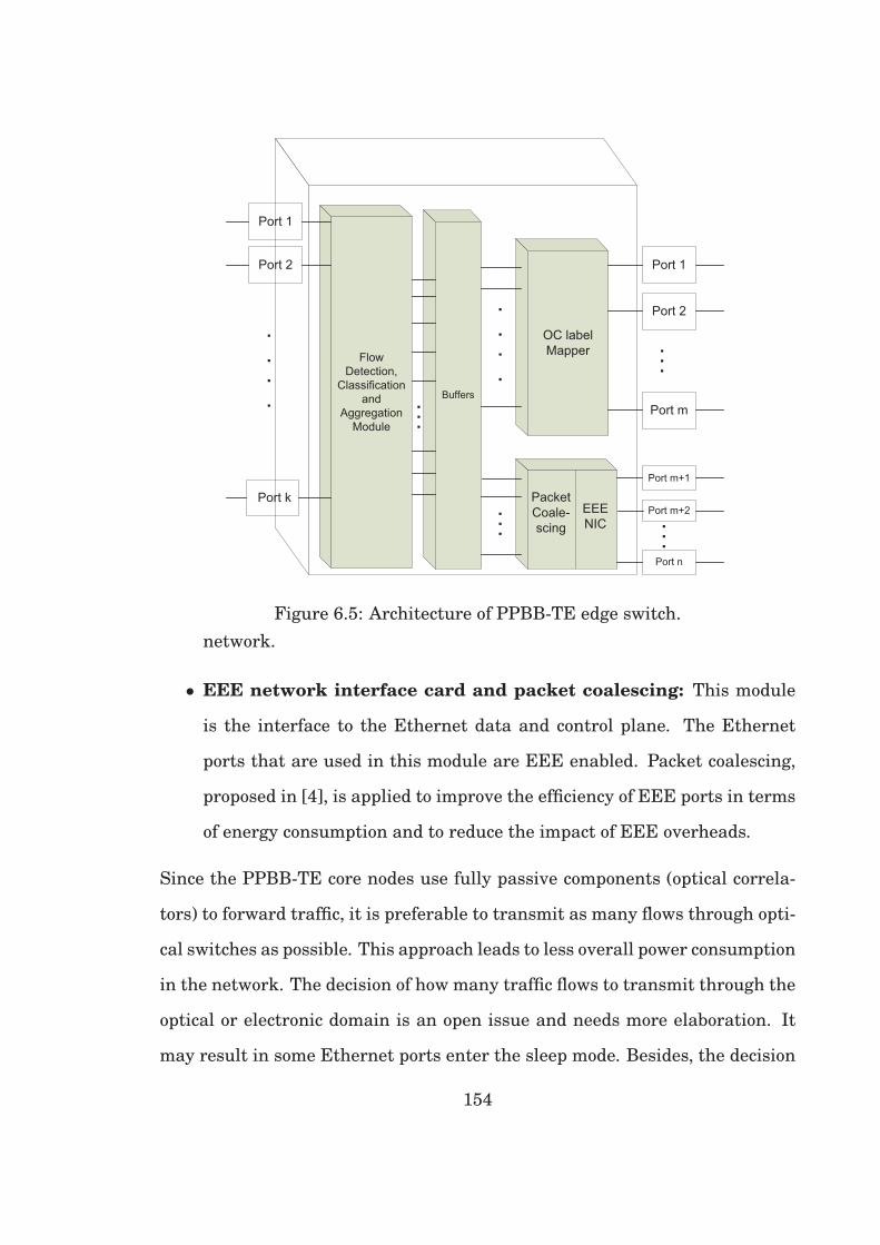
Figure 6.5: Architecture of PPBB-TE edge switch.network.

• EEE network interface card and packet coalescing: This module

is the interface to the Ethernet data and control plane. The Ethernet

ports that are used in this module are EEE enabled. Packet coalescing,

proposed in [4], is applied to improve the efficiency of EEE ports in terms

of energy consumption and to reduce the impact of EEE overheads.

Since the PPBB-TE core nodes use fully passive components (optical correla-

tors) to forward traffic, it is preferable to transmit as many flows through opti-

cal switches as possible. This approach leads to less overall power consumption

in the network. The decision of how many traffic flows to transmit through the

optical or electronic domain is an open issue and needs more elaboration. It

may result in some Ethernet ports enter the sleep mode. Besides, the decision

154

to put Ethernet ports into the sleep mode needs to be taken carefully due to

the transition overhead associated with it. We address this problem of EEE

transition overhead in Section 6.3.

6.3 Energy-Aware scheduling

The recent standard IEEE 802.3az EEE enhance the usability of Ethernet net-

works by being more energy efficient. However, EEE may suffer from a signif-

icant overhead stemming from the wake time (tw) and sleep time (ts) without

a suitable scheduling of incoming frames which will impact on overall energy

consumption (see Section 6.1.2 for further detail). Packet coalescing [4] as pro-

posed lacks an efficient mechanism for scheduling the transmission times of

Ethernet frames; that is, properly selecting the active intervals during which

the frames will be transmitted on each port. Recall that in packet coalesc-

ing, a transmission timer is essentially set for each port; once this timer ex-

pires, all packets which have accumulated so far will be bursted out at line

speed. Indeed, the selection of the timer plays a critical role in trading off the

power consumption of the port and the delay experienced by the frames at each

port. Hence, scheduling the activation events of the ports will be crucial in re-

ducing power consumption as well as guaranteeing quality-of-service (QoS) in

the network, in terms of end-to-end delay that frames will experience. Next,

we present an illustrative example to explain the importance of scheduling in

greater detail.

155

6.3.1 Illustrative Example

We consider a simple instance where five frames f1, f2, f3, f4, and f5 of dif-

ferent sizes with various delay thresholds arrive at times 3, 5, 8, 9, and 10

respectively (see Table 6.1). Table 6.1 presents other parameters used in this

illustrative example, such as the size and delay requirement for each frame

and transmission time of frames. The transmission time of a frame is com-

puted under the assumption of a link rate of 10 Gb/s. For illustrative purpose,

we assume two EEE ports (p1 and p2) are available to transmit these frames.

Frames f1 f2 f3 f4 f5Arrival (unit time) 3 5 8 9 10Size (Bytes) 1500 1500 1250 1250 750Transmission time (μsec) 1.2 1.2 1 1 0.6assuming 10 Gb/s linkDelay (unit time) 7 6 6 3 3

Table 6.1: Parameter values

Fig. 6.6 demonstrates two different but possible scheduling alternatives

that can be adopted, which work as follows. Fig. 6.6(a), referred to as Schedul-

ing 1, assumes that the timer expires at time instant 9. At this time, frames

f1, f2, and f3 are in the buffer and will start their transmission through port

p1. Thus, port p1 will be in busy state from time 9 to 12.4 while transmitting

frames f1, f2, and f3, as depicted in Fig. 6.6(a)-(ii). When frame f4 arrives

at time 9 with delay threshold 3, this frame (f4) must be transmitted at time

instant 12 the latest. Since p1 is in busy state until time 12.4, the scheduler

needs to activate port p2 to transmit f4 and satisfy its delay requirement. Next,

frame f5 arrives at time 10 and can be transmitted through either port p1 or

p2. A possible scenario of transmission of frames f4 and f5 is presented in Fig.

6.6(a)-(iii). An alternative scenario for scheduler 1 is to transmit frame f4 at

time 9, subsequently followed by frame f5 through port p2, as shown in Fig.

156

(b) Scheduling 2(a) Scheduling 1

91011121314

10.211.412.4

p1

(ii)

13.6

p2

91011121314

(iii)

(i)

Active

interval start

6

f5

358910

Time

p1

p2

67891011

7.28.49.410.4

(ii)

f1

f2

f3

f4

f5

p1

p2

91011121314

11.4 10.212.4

10.6

(iv)

Active

interval start

9

358910

Time

(i)

f1

f2

f3

f5

f5

f4

f3

f2

f1

f4

f4

f5

f1

f2

f3

f4

f5

f1

f2

f3

Figure 6.6: Scheduling options for a simple instance.6.6(a)-(iv) to reduce the average delay of those frames. Notice that in both

cases, scheduling 1 requires the activation of two ports. Fig. 6.6(b) illustrates

an alternative schedule, referred to as Scheduling 2, where port p1 is activated

at time instance 6 to transmit frames f1 and f2. When frame f3 arrives at

time 8, it is scheduled at time 8.4 on the same port p1. Similarly, frames f4

and f5 are scheduled for transmission on port p1 at time instance 9.4 and 10.4

respectively, as depicted in Fig. 6.6(b)-(ii). Clearly, this transmission schedule

is able to transmit all frames within their deadlines using only one port, while

keeping the second port p2 in LPI mode and thus conserving more energy. It is

therefore clear that efficiently deciding the transmission schedules is key to re-

duce energy consumption while meeting the delay requirements of the traffic.

Next, we present a mathematical model that achieves this objective.

157


In this section, we formulate the problem of energy-aware scheduling of Ether-

net frames as a Mixed Integer Linear Program (MILP); the MILP determines

the optimal transmission schedule at the ports, which both guarantees the de-

lay requirement of the incoming frames and reduces the energy consumption

by minimizing the period of active time of the ports. For the purpose of our

model, we assume the knowledge of the traffic profile at each port; that is, the

total number of frames F , the size of each frame zf (bytes), and their arrival

times are also assumed to be known in a window of time W . We further as-

sume that the frames should be scheduled using a certain number of active

intervals at each port and we let I be the maximum number of intervals re-

quired for completing the transmission of all the frames. Each frame has its

own delay threshold parameter df and thus needs to be transmitted before df .

Let us assume that the number of available EEE ports is P , each with the ca-

pacity of Cp (bps). Let xp,if be a binary variable, which denotes whether frame

f is scheduled for transmission during an active interval i on port p (xp,if = 1)

or not (xp,if = 0). Similarly, let yip be a binary variable denoting whether port p

is turned on during active interval i (yip = 1) or not (yip = 0). sip and eip are the

start and end times of active interval i of port p, respectively. rf is the release

time of frame f . The other variables are defined as follows.

trip : Transmission time in active interval i on port p.

tactivep : Total active duration of port p in time window W .

δon : Unit energy consumption of a port when it is on.

tw : Wake-up time of a port. The value is 4.48μs for 10 Gb/s Ethernet in IEEE

standard 802.3az [4].

δw : Unit energy consumption of a port while waking up.

158

ts : Sleep transition time of a port. The value is 2.88μs for 10 Gb/s Ethernet in

IEEE standard 802.3az [4].

δs : Unit energy consumption of a port while going to sleep.

tidlep : Total idle duration of port p in time window W .

δidle : Unit energy consumption of a port when idle. It can be as low as 10

percent of δon [4].

Ep : Total energy consumption of port p in time window W .

The objective of our model is to minimize the energy consumption when trans-

mitting all the frames backlogged at each port p during a period of time W .

MinP∑

p=1

Ep (6.1)

s.t.

Ep = tidlep × δidle +I∑

i=1

[yip × (tw × δw + ts × δs) + trip × δon] (6.2)

tidlep = W − tactivep (6.3)

tactivep =I∑

i=1

[yip × (tw + ts) + trip] ∀p (6.4)

Constraint (6.2) represents the energy consumption per port p taking into ac-

count the total idle time and active period during the whole scheduling period

consisting of all intervals I, where (6.3) and (6.4) determine the idle and active

period at port p.P∑

p=1

I∑i=1

xp,if = 1 ∀ f (6.5)

xp,if ≤ yip ∀ f, p, i (6.6)

159

Constraints (6.5) and (6.6) ensure that each frame is transmitted at most once

through an active port. More precisely, constraint (6.5) determines that a

frame f must be scheduled on only one port during only one active interval.

Constraint (6.6) will activate a port p if a frame is scheduled on that port.

rf ≥ af ∀ f (6.7)

rf − af ≤ df ∀ f (6.8)

rf ≤ sip +M(1− xp,if ) ∀ f, p, i (6.9)

rf ≥ sip −M(1− xp,if ) ∀ f, p, i (6.10)

Constraints (6.7) to (6.10) define the boundary conditions of release time of a

frame and the delay threshold of the frame is guaranteed by Equation (6.8).

M is a large constant.

sip ≤ eip (6.11)

eip − sip = trip (6.12)

trip ≥ (F∑

f=1

xp,if × zf )/Cp (6.13)

trip ≤ M(yip) (6.14)

eip ≤ W ∀p, i (6.15)

Constraints (6.11) to (6.15) define the duration and bound of active intervals

of each port. The duration of an active interval is estimated by the required

transmission time of the frames that are scheduled for transmission during

160

that interval. Constraint (6.16) imposes a minimum space between two con-

secutive active intervals of port p.

sip − ejp ≥ ts + tw −M(1− yip)−M(1− yjp) ∀ p and j < i (6.16)

6.3.3 Sequential Fixing

The mathematical formulation of energy aware scheduling is clearly a com-

binatorially complex decision problem and does not scale for larger problem

instances. To reduce the running time, we develop and implement a heuristic

based on Sequential Fixing approach (SF). In our model, the binary variable

xp,if indicates whether the port p is used by the frame f in time interval i. In

our sequential fixing method, we relax the integrality of xp,if (xp,i

f ∈ [0, 1]) and

solve the corresponding modified MILP model. For each frame f , we find the

maximum value of xp,if and identify the value of corresponding p and i, which

indicates the port and interval number, respectively. We fix the value of that

particular xp,if to 1 and solve the modified model. If a feasible solution can be

reached by this modification, the heuristic moves forward to the next frame.

Otherwise, the value of xp,if is set to 0 and the model is solved. This process

continues as long as the heuristic finds a feasible solution for current frame.

The heuristic iterates until the values of xp,if turn into binaries.

6.4 Numerical Results

The authors of [58] and [4] evaluated the performance of EEE and packet co-

alescing on EEE ports. They showed that EEE can significantly reduce the

161

10 20 30 40 50 60 700

20

40

60

80

100

% Link utilization

Nor

mal

ized

ene

rgy

cons

umpt

ion

OMMC1MC2EEEno EEE

Figure 6.7: Energy consumption vs. link utilization

energy consumption of conventional Ethernet links and packet coalescing de-

creases the EEE overhead and thus reduces the energy consumption further.

However, the energy efficiency is achieved in packet coalescing at the expense

of an increased end-to-end delay. In this section, we evaluate the performance

of our energy-aware optimal scheduling model. The objective is to compare the

optimal results to the results achieved in [58] and [4]. The proposed energy-

aware scheduling model is implemented in C++ and solved using CPLEX Con-

cert Technology.

6.4.1 Comparison of MILP with existing approaches

Conventional Ethernet referred to as “no EEE” operates at maximum power

all the time and thus consumes 100% of energy, regardless of the link utiliza-

tion. In EEE, a link becomes active upon the arrival of a frame and enters the

LPI mode when there is no frame to transmit. For fair comparison, the heuris-

tic of packet coalescing [4] is modified to incorporate delay thresholds of the

162

frames, referred to as “MC”. In addition to the timer and frame counter, MC

activates the link as soon as the delay threshold of a frame is about to expire

and transmits the accumulated frames. The energy-aware optimal scheduling

model is referred to as “OM”. The heuristic with relaxed model is referred to

as “SF”. γ represents the link utilization in percentage. All the experiments

are performed on a 1 Gb/s Ethernet link and frames are assumed to arrive at

the incoming link according to a Poisson process. We assume that the power

consumption of EEE in LPI mode be 10 percent of that in the active mode

specified in IEEE standard 802.3az. We further assume that EEE consume 90

percent of the active energy during its transition from active to LPI or LPI to

active mode.

Fig. 6.7 demonstrates the normalized energy consumption of EEE over a

range of link utilization. Two blocks labeled as MC1 and MC2 show the re-

sults for MC with timer set to 3 μs and frame counter set to 2 frames, and

with timer set to 5 μs and frame counter set to 4 frames, respectively. The

delay thresholds and size of the frames are generated randomly with mean

value of 115 μs and 1250 bytes, respectively. The figure clearly shows that the

model yields minimum energy consumption comparing to MC1, MC2 and EEE

all achieving close performance. This indeed shows that the proposed con-

cepts (Packet coalescing and EEE) are promising approaches for deployment

in backbone switches to reduce energy consumption. It is to be mentioned that

these performances are obtained for fewer number of frames; this is due to the

prohibitively large running time of the optimization model with larger number

of frames. However, we expect that performance will change as we increase the

load.

Table 6.2 presents the average delay(μs) of the transmitted frames versus

163

10 20 30 40 50 60 70 80 90 100

101.4

101.6

101.8

% Link utilization

Nor

mal

ized

ene

rgy

cons

umpt

ion

EEEMC

Figure 6.8: Energy consumption vs. link utilization

link utilization. In terms of delay performance, we note that all frames are

scheduled within their delay requirements in all methods. The model how-

ever resulted in larger delays since our objective is simply to minimize energy

consumption. EEE, as opposed to MC, results in better delay performance in

both (fewer and larger number of frames) cases. Please note, however, that the

frame delays are measured in micro-seconds and hence these increases remain

acceptable and comparable.

γAverage Delay (μs)

OM SF MC1 MC2 EEE No EEE10 63.25 37.62 15.38 9.080 4.88 0.020 51.93 29.75 16.02 9.274 5.85 0.9730 55.29 44.54 15.76 9.418 4.82 0.4240 64.95 62.84 16.18 9.720 6.04 1.71

Table 6.2: Avg. delay vs. link utilization

Fig. 6.8 presents the performance evaluation of EEE and MC with larger

amount of frames which exhibits that MC yields substantial performance im-

provement (reduction in energy up to 47.6% in some cases) over EEE. This

is consistent with the findings of [58] and provides the reasoning of our ex-

pectations. However, both of their performance traces predictably converge at

excessive link utilization (100%). This is because, in high utilization, frames

164

arrive very near to each other and mostly merge to the transmission time of

each other, thus, reduces the number of EEE transition from one mode to other.

6.4.2 Optimization model and sequential fixing

To overcome the limitations of expensive running time of the model, we de-

velop a heuristic as explained in Section 6.3.3. Fig. 6.10 compares the energy

consumption achieved by OM and the heuristic SF. Fig. 6.9 presents the CPU

time required to execute OM and SF with various link utilizations. The results

show a substantial decrease in running time by the SF especially after 40% of

link utilizations. However, the results of the objective function, i.e., energy

consumption achieved by the SF is very near to the optimal values achieved

by the OM. More precisely, 7 out of 10 instances achieved the optimal results

by SF as presented in Fig. 6.10. The rest of the three instances are 0.6% to

1% apart from the optimal results. Thus SF can be a legitimate alternative of

OM which can provide the opportunity to evaluate the performance in larger

instances.

6.4.3 Impact of frame delay and sizes on the energy con-

sumption

We further study the impact of delay and frame size in energy consumption

and thus execute the experiments with SF by varying the delays and frame

sizes as presented in Figs 6.11, 6.12, and 6.13. Four different delay ranges (50-

70)μs, (70-90)μs, (90-110)μs, and (110-130)μs are examined in various link uti-

lizations. Frame sizes are varied between (500-1000)bytes, (1000-1500)bytes,

and (1500-2000)bytes in various link utilizations. Please note that, though the

maximum size of Ethernet frames are 1500 bytes, we intentionally increase

165

10 20 30 40 50 60 70 80 90 10010−2

100

102

104

106

Link utilization (%)

CPU

Tim

e (s

ec)

OMSF

Figure 6.9: CPU time of OM vs. SF

the size of the frames over 1500 bytes1 to observe the effect on energy con-

sumption. It is trivial to predict that the energy consumption will be higher

for larger frame sizes because of the longer transmission times. However, this

should not be considered as a downside and more importantly energy efficiency

need to be observed in this case. Energy efficiency (η) can be defined as the

transmission time over total active time, i.e., (transmission time + EEE tran-

sition overhead). The higher value for energy efficiency indicates more energy

is used in actual data transmission and less energy is consumed during EEE

mode transition.

Fig. 6.11 presents the unit energy consumption of four delay variations.

Since the tighter delay bound may force the scheduler to activate more ports,1Although this exceeds the maximum size of Ethernet frames.

166

10 20 30 40 50 60 70 80 90 1000

100

200

300

400

500

600

700

800

900


Ener

gy c

onsu

mpt

ion

OMSF

Figure 6.10: Energy consumption of OM vs. SF

understandably the results in Fig. 6.11 show that an increase in delay re-

quirements can reduce energy consumption. Fig. 6.12 and 6.13 illustrates the

comparisons of unit energy consumption and energy efficiency of three varia-

tions of frame sizes in different link utilizations. Predictably increase in frame

size results in more energy consumption as presented in Fig. 6.12. However,

the more interesting observation is that higher energy efficiency is achieved

by increasing frame sizes as presented in Fig. 6.13, which states that energy

is consumed more efficiently in larger frame sizes and desirably more energy

is consumed in active data transmission over EEE overhead with larger frame

sizes.

167

10 20 30 40 50 60 70 80 90 100

103.3

103.4

103.5

103.6

103.7


Ener

gy c

onsu

mpt

ion

Delay (50−70)Delay (70−90)Delay (90−110)Delay (110−130)

Figure 6.11: Energy consumption with varying delay range

6.5 Chapter remark

The ratification of the IEEE 802.1Qay PBB-TE increases the suitability of Eth-

ernet in carrier transport networks. The new IEEE 802.3az Energy Efficient

Ethernet will certainly help the service providers to proceed towards green

transport networks. Photonic PBB-TE switches can increase the usability of

PBB-TE networks further and can reduce power consumption by leveraging

EEE. The proposed energy-aware scheduling optimization model provides a

benchmark of energy efficiency and the heuristic with relaxed model can be

greatly helpful to analyze the trade-offs between energy efficiency and latency

in the networks. In this chapter, we studied the trade-off with guaranteed

frame transmission within its delay requirement and the effect of various pa-

rameters such as delay range and frame sizes on energy consumption. It is

evidenced from experimental results that lower delay tolerant traffic consume

168

10 20 30 40 50 60 70 80 90 1000

1000

2000

3000

4000

5000

6000

7000


Ener

gy c

onsu

mpt

ion

Frame Size (500−1000)Frame Size (1000−1500)Frame Size (1500−2000)

Figure 6.12: Energy consumption with varying frame size

up to 5% more energy than that of flexible traffic and the larger frames con-

sume energy up to 31% more efficiently.

169

10 20 30 40 50 60 70 80 90 1000.55

0.6

0.65

0.7

0.75

0.8

0.85

0.9

0.95


Ener

gy e

ffic

ienc

y (%

)

Frame size (500−1000)Frame size (1000−1500)Frame size (1500−2000)

Figure 6.13: Energy efficiency with varying frame size

170

Chapter 7

Conclusion and Future

Directions

7.1 Conclusions

This thesis addressed two important design aspects of carrier Ethernet net-

works, namely, (i) survivable Ethernet transport networks design using a fast

restorable protection mechanism and (ii) design of a green Ethernet transport

network using Energy Efficient Ethernet (EEE).

We first presented a survivable network design approach for Ethernet trans-

port networks using Ethernet Ring Protection (ERP) protocol. We identified

some subtle limitations of prior work which used a computationally expensive

exhaustive enumeration approach for determining the best RPL locations and

the best ring hierarchies. We then developed a modified routine to overcome

those limitations. We developed an ILP model for optimal resource allocation

in single ring networks as well as in multi-ring mesh networks by properly

selecting the RPL placements and ring hierarchies. Unlike that prior work

which sequentially selects the ring hierarchy and the RPL location one after

171

another, our model jointly determine the RPL placements and the ring hierar-

chies while minimizing the capacity requirements. In this work, the network

is designed to survive against any single link failure only.

We then extended our ERP-based network design approach by consider-

ing concurrent dual link failures scenarios. We showed that network services

may suffer two types of service outages due to concurrent dual link failures

in an Ethernet network which is protected by ERP protocol. One is for net-

work partitioning (physical/logical) which we referred to as category-1 outages

and category-2 outages are referred to as the service outages that are suffered

from lack of capacity. First, we developed an optimization model to minimize

the category-1 service outages by efficient selection of the RPL placements and

ring hierarchies. We also developed a routine to estimate the additional capac-

ity requirement to eliminate category-2 outages. This two-step approach can-

not guarantee optimal capacity allocation. We formally proved that a network

designed with the objective of maximizing network flows ultimately minimizes

both categories of service outages caused by dual link failures. Then we devel-

oped another optimization model which jointly minimizes both categories of

service outages by maximizing network flows while minimizing capacity re-

quirements.

We then presented the ERP-based mesh networks design from a different

perspective which is more practical from network operators point of view, i.e.

traffic engineering approach. We mathematically formulated the ERP design

problem for a network with fixed capacity with the objective of fair distribution

of network resources among the given traffic sessions, hence avoiding conges-

tion in some parts of the network while other parts remained under-utilized.

Then, we exploited one of the advantageous features of ERP protocol which

172

is the ability to deploy multiple logical ERP instances over a single physical

ring. We developed a design model which provides the best possible set of ERP

instances to be implemented with their RPLs and ring hierarchies.

Finally, we presented a carrier Ethernet network architecture which is ex-

pected to be energy efficient. We designed the architectures of two novel Eth-

ernet switches: the core switch is equipped with passive optical correlators for

optical packet bypassing and the edge switch is equipped with newly standard-

ized Energy Efficient Ethernet (EEE) ports. We then developed an optimiza-

tion model to minimize energy consumption in EEE ports by efficient schedul-

ing of Ethernet frames. The scheduling problem turned out to be a combinato-

rially complex problem and thus unsolvable for large number of frames. Thus,

we developed a heuristic based on sequential fixing technique and obtained

very near to optimal solutions in faster time.

7.2 Future Work

The work presented in this thesis provided considerable amount of insight

for survivable Ethernet transport network design using the promising ERP

protocol. However, there remain several future research works of immense

interest, especially in the context of newly emerging data-center networks.

The design strategies of ERP-based mesh networks that are presented in

this thesis considered only E-line services or point-to-point Ethernet virtual

connections. However, E-tree services and point-to-multipoint virtual connec-

tions are more suitable for providing emerging data-center services. Hence, in

order to provision protection plans using ERP for data-center based networks

require particular attention and further research.

173

The design strategies of this thesis, in particular the design model for mul-

tiple ERP instances requires further research to improve its scalability. Large

scale optimization methods or efficient meta-heuristic methods might be help-

ful to make the model more scalable.

In this thesis, we only considered simple physical rings of mesh networks to

configure single or multiple ERP instances. However, further research could be

performed to investigate the benefit of considering all possible physical rings

and then select the best set of physical rings to implement ERP. This research

direction has immense potential to improve the performance of ERP dramati-

cally.

174

Bibliography

[1] MEF, “Carrier Ethernet Services Overview.” [On-

line]. Available: http://www.metroethernetforum.

org/PPT Documents/Reference-Presentation%s/Nov-2011/

Carrier-Ethernet-Services-Overview-Reference-Presentation-R03-2011-11-15.

ppt%x

[2] D. Allan, N. Bragg, A. Mcguire, and A. Reid, “Ethernet as carrier trans-

port infrastructure,” IEEE Communications Magazine, vol. 44, no. 2, pp.

95 – 101, feb. 2006.

[3] ITU-T Rec. G.8032/Y.1344, “Ethernet ring protection switching,” 2012.

[4] K. Christensen et al., “IEEE 802.3az: The Road to Energy Efficient Eth-

ernet,” IEEE Communications Magazine, vol. 48, no. 11, pp. 50 –56, Nov.

2010.

[5] Infonetics Research, “Service providers capitalize on Ethernet and IP

MPLS VPN services,” Jul 2011.

[6] ——, “Service Provider Plans for Metro Optical and Ethernet: North

America, Europe, and Asia Pacific 2007,” Sep 2007.

175

[7] IEEE, “IEEE Standard for Local and metropolitan area networks: Media

Access Control (MAC) Bridges,” IEEE Std 802.1D-2004 (Revision of IEEE

Std 802.1D-1998), pp. 1–277, 9 2004.

[8] ——, “IEEE Standards for Local and Metropolitan Area Networks— Vir-

tual Bridged Local Area Networks— Amendment 3: Multiple Spanning

Trees,” IEEE Std 802.1s-2002 (Amendment to IEEE Std 802.1Q, 1998

Edition), pp. 1–211, 2002.

[9] ——, “IEEE Standard for Local and Metropolitan Area Networks - Com-

mon Specification. Part 3: Media Access Control (MAC) Bridges - Amend-

ment 2: Rapid Reconfiguration,” IEEE Std 802.1w-2001, 2001.

[10] K. Fouli and M. Maier, “The Road to Carrier-Grade Ethernet,” IEEE Com-

munications Magazine, vol. 47, no. 3, pp. S30–S39, Mar 2009.

[11] A. KIRSTADTER, C. GRUBER, J. RIEDL, and T. BAUSCHERT, “Carrier-

grade ethernet for packet core networks,” in Proceedings of SPIE, the In-

ternational Society for Optical Engineering. Society of Photo-Optical In-

strumentation Engineers, 2006.

[12] MEF, “service provider study: Operating expenditures”.” [On-

line]. Available: ”http://metroethernetforum.org/PDF Documents/

Provider-Business-Case-OpEx-Study-Summary old.pdf”

[13] M. Huynh and P. Mohapatra, “Metropolitan ethernet network: A move

from lan to man,” Computer Networks, vol. 51, no. 17, pp. 4867 – 4894,

2007.

176

[14] A. Kern, I. Moldovan, and T. Cinkler, “Bandwidth guarantees for resilient

ethernet networks through rstp port cost optimization,” in International

Conference on Access Networks Workshops, Aug. 2007, pp. 1 –8.

[15] M. Marchese, M. Mongelli, and G. Portomauro, “Simple protocol enhance-

ments of rapid spanning tree protocol over ring topologies,” in IEEE

GLOBECOM, Dec. 2010, pp. 1–5.

[16] E. Bonada and D. Sala, “Rstp-sp: Shortest path extensions to rstp,” in

International Conference on High Performance Switching and Routing,

Jun 2012, pp. 223 –228.

[17] G. Ibanez, A. Garcia, and A. Azcorra, “Alternative multiple spanning tree

protocol (amstp) for optical ethernet backbones,” in IEEE International

Conference on Local Computer Networks, nov. 2004, pp. 744 – 751.

[18] A. De Sousa, “Improving load balance and resilience of ethernet carrier

networks with ieee 802.1s multiple spanning tree protocol,” in Interna-

tional Conference on Systems and Networking, Apr. 2006, p. 95.

[19] A. Meddeb, “Multiple spanning tree generation and mapping algorithms

for carrier class ethernets,” in IEEE GLOBECOM, Dec. 2006, pp. 1 –5.

[20] H. T. Viet, Y. Deville, O. Bonaventure, and P. Francois, “Traffic engineer-

ing for multiple spanning tree protocol in large data centers,” in Interna-

tional Teletraffic Congress (ITC), Sept. 2011, pp. 23–30.

[21] M. Fine, S. Gai, and K. McCloghrie, “Shared spanning tree protocol,” Feb

2001, uS Patent 6,188,694.

177

[22] J. Im, J. Ryoo, and J. Rhee, “Managed FDB algorithm and protection in

ethernet ring topology,” in Joint International Conference on Optical In-

ternet and Australian Conference on Optical Fibre Technology, June 2007,

pp. 1 –3.

[23] K. Lee, J.-K. Rhee, S. Yoo, and P. Cho, “Flush optimization in ether-

net ring protection network,” in International Conference on ICT Conver-

gence, Sept. 2011, pp. 513 –514.

[24] K. Lee, J. Ryoo, and S. Min, “An Ethernet ring protection method to min-

imize transient traffic by selective FDB advertisement,” ETRI journal,

vol. 31, no. 5, pp. 631–633, 2009.

[25] J. Rhee, J. Im, and J. Ryoo, “Ethernet ring protection using filtering

database flip scheme for minimum capacity requirement,” Etri Journal,

vol. 30, no. 6, pp. 874–876, 2008.

[26] K. Lee, C. Lee, and J. Ryoo, “Enhanced protection schemes to guarantee

consistent filtering database in Ethernet rings,” in IEEE GLOBECOM,

Dec. 2010, pp. 1 –6.

[27] D. Lee, J.-K. Rhee, K. Lee, and P. Cho, “Efficient Ethernet multi-ring pro-

tection system,” in International Workshop on Design of Reliable Commu-

nication Networks, Oct. 2009, pp. 305 –311.

[28] D. Lee, K. Lee, S. Yoo, and J.-K. Rhee, “Efficient ethernet ring mesh net-

work design,” Journal of Lightwave Technology, vol. 29, no. 18, pp. 2677

–2683, Sept. 15 2011.

178

[29] K.-k. Lee, J.-d. Ryoo, S. H. Kim, and D. Kim, “An optimal Ring-Protection-

Link positioning algorithm in carrier Ethernet ring networks,” IEEE

Communications Letters, vol. 16, no. 8, pp. 1332 –1335, Aug 2012.

[30] K. Lee, D. Lee, H.-w. Lee, N.-g. Myoung, Y. Kim, and J.-K. Rhee, “Reliable

network design for ethernet ring mesh networks,” Journal of Lightwave

Technology, vol. 31, no. 1, pp. 1 –9, Jan. 2013.

[31] L. K.-k, J.-d. Ryoo, S. Kim, and J. Lee, “Effective load balancing in eth-

ernet rings,” in IEEE Network Operations and Management Symposium,

April 2012, pp. 482 –485.

[32] S. Taniguchi, K. Kitayama, Y. Baba, and H. Yamanaka, “Detection and re-

covery of the blocked ports defect for the reliable ethernet ring protection

switching,” in 15th OptoeElectronics and Communications Conference, Jul

2010, pp. 572 –573.

[33] K.-K. Lee and J.-D. Ryoo, “Flush optimizations to guarantee less transient

traffic in ethernet ring protection,” ETRI Journal, vol. 32, pp. 184–194,

Apr. 2010.

[34] R. Ramaswami, K. Sivarajan, and G. Sasaki, Optical Networks: A Prac-

tical Perspective, 3rd Edition, 3rd ed. San Francisco, CA, USA: Morgan

Kaufmann Publishers Inc., 2009.

[35] M. Nurujjaman, S. Sebbah, C. Assi, and M. Maier, “Optimal capacity plan-

ning and RPL placement in carrier ethernet mesh network design,” in

IEEE International Conference on Communications, Jun. 2012.

[36] M. Clouqueur and W. Grover, “Availability analysis of span-restorable

mesh networks,” IEEE JSAC, vol. 20, no. 4, pp. 810–821, May 2002.

179

[37] T. Leighton and S. Rao, “Multicommodity max-flow min-cut theorems and

their use in designing approximation algorithms,” Journal of the ACM

(JACM), vol. 46, no. 6, pp. 787–832, Nov. 1999.

[38] M. Allalouf and Y. Shavitt, “Centralized and distributed algorithms for

routing and weighted max-min fair bandwidth allocation,” IEEE/ACM

Transactions on Networking, vol. 16, no. 5, pp. 1015 –1024, oct. 2008.

[39] L. Tan, X. Zhang, L. Andrew, S. Chan, and M. Zukerman, “Price-based

max-min fair rate allocation in wireless multi-hop networks,” IEEE Com-

munications Letters, vol. 10, no. 1, pp. 31 – 33, jan 2006.

[40] A. Reid et al., “Carrier Ethernet,” IEEE Communications Magazine,

vol. 46, no. 9, pp. 96–103, Sep. 2008.

[41] A. Takacs, H. Green, and B. Tremblay, “GMPLS Controlled Ethernet:

An Emerging Packet-Oriented Transport Technology,” IEEE Communi-

cations Magazine, vol. 46, no. 9, pp. 118–124, Sep. 2008.

[42] D. Fedyk, H. Shah, N. Bitar, and A. Takacs, “Generalized Multiprotocol

Label Switching (GMPLS) control of Ethernet PBB-TE,” IETF Internet

Draft, Oct. 2009, work in progress.

[43] A. Takacs, B. Gero, D. Fedyk, D. Mohan, and H. Long, “GMPLS RSVP-TE

Extensions for Ethernet OAM Configuration,” IETF Internet Draft, Oct.

2009, work in progress.

[44] F. Farnoud, M. Ibrahimi, and J. A. Salehi, “A Packet-Based Photonic La-

bel Switching Router for a Multirate All-Optical CDMA-Based GMPLS

Switch,” IEEE Journal of Selected Topics in Quantum Electronics, vol. 13,

no. 5, pp. 1522–1530, Sept./Oct. 2007.

180

[45] R. Tucker, R. Parthiban, J. Baliga, K. Hinton, R. Ayre, and W. Sorin, “Evo-

lution of WDM optical ip networks: A cost and energy perspective,” Jour-

nal of Lightwave Technology, vol. 27, no. 3, pp. 243 –252, 2009.

[46] TPACK, “P-OTN: Packet Optical Network Transformation,” 2008.

[47] K. Kitayama and N. Wada, “Photonic IP Routing,” IEEE Photonics Tech-

nology Letters, vol. 11, no. 12, pp. 1689–1691, Dec. 1999.

[48] IETF, “OSPF Extensions in support of Generalized Multi-Protocol Label

Switching (GMPLS),” IETF RFC 4203, Oct. 2005.

[49] ——, “Routing Extensions in Support of Generalized Multi-Protocol Label

Switching (GMPLS),” IETF RFC 4202, Oct. 2005.

[50] ——, “Generalized Multi-Protocol Label Switching (GMPLS) Signaling

Resource ReserVation Protocol-Traffic Engineering (RSVP-TE) Exten-

sions,” IETF RFC 3473, Jan. 2003.

[51] D. Awduche, L. Berger, D. Gan, T. Li, V. Srinivasan, and G. Swallow,

“RSVP-TE: Extensions to RSVP for LSP Tunnels,” IETF RFC 3209, Dec.

2001.

[52] K. Fouli and M. Maier, “OCDMA and Optical Coding: Principles, Appli-

cations, and Challenges,” IEEE Communications Magazine, vol. 45, no. 8,

pp. 27–34, Aug. 2007.

[53] T. Khattab and H. Alnuweiri, “Optical CDMA for All-Optical Sub-

Wavelength Switching in Core GMPLS Networks,” IEEE Journal on Se-

lected Areas in Communications, vol. 25, no. 5, pp. 905–921, 2007.

181

[54] M. Murata and K. Kitayama, “A Perspective on Photonic Multiprotocol

Label Switching,” IEEE Network, vol. 15, no. 4, pp. 56–63, 2001.

[55] G.-K. Chang et al., “Enabling Technologies for Next-Generation Optical

Packet-Switching Networks,” Proceedings of the IEEE, vol. 94, no. 5, pp.

892–910, May 2006.

[56] L. G. Roberts, “A Radical New Router,” IEEE Spectrum, vol. 46, no. 7, pp.

34–39, Jul. 2009.

[57] N. Kataoka, N. Wada, G. Cincotti, K. Kitayama, and T. Miyazaki, “A novel

multiplexed optical code label processing with huge number of address

entry for scalable optical packet switched network,” 33rd European Con-

ference and Ehxibition of Optical Communication (ECOC), pp. 1–2, Sept.

2007.

[58] P. Reviriego et al., “Performance Evaluation of Energy Efficient Ethernet,”

IEEE Communication Letters, vol. 13, pp. 697–699, Sept. 2009.

182