optimal demand response: problem formulation and...
TRANSCRIPT

Optimal demand response: problem formulationand deterministic case
Lijun Chen, Na Li, Libin Jiang, and Steven H. Low
Abstract We consider a set of users served by a single load-serving entity (LSE).The LSE procures capacity a day ahead. When random renewable energy is re-alized at delivery time, it manages user load through real-time demand responseand purchases balancing power on the spot market to meet the aggregate demand.Hence optimal supply procurement by the LSE and the consumption decisions bythe users must be coordinated over two timescales, a day ahead and in real time,in the presence of supply uncertainty. Moreover, they must be computed jointly bythe LSE and the users since the necessary information is distributed among them. Inthis paper we present a simple yet versatile user model and formulate the problemas a dynamic program that maximizes expected social welfare. When random re-newable generation is absent, optimal demand response reduces to joint schedulingof the procurement and consumption decisions. In this case, we show that optimalprices exist that coordinate individual user decisions to maximize social welfare,and present a decentralized algorithm to optimally schedule a day in advance theLSE’s procurement and the users’ consumptions. The case with uncertain supply isreported in a companion paper.
1 Introduction
1.1 Motivation
There is a large literature on various forms of load side management from the classi-cal direct load control to the more recent real-time pricing [1, 2]. Direct load control
Lijun Chen, Na Li, Libin Jiang and Steven H. LowEngineering and Applied Science, California Institute of Technology, USAe-mail: {chenlj, nali, libinj, slow}@caltech.eduTo appear: In Control and Optimization Theory for Electric Smart Grids. AranyaChakrabortty and Marija Ilic, Editors, Springer 2011
1

2 Lijun Chen, Na Li, Libin Jiang, and Steven H. Low
in particular has been practised for a long time and optimization methods have beenproposed to minimize generation cost e.g. [3, 4, 5, 6], maximize utility’s profit e.g.[7], or minimize deviation from users’ desired consumptions e.g. [8, 9], sometimesintegrated with unit commitment and economic dispatch e.g. [4, 10]. Almost all de-mand response programs today target large industrial or commercial users, or, inthe case of residential users, a small number of them, for two, among other, impor-tant reasons. First, demand side management is invoked rarely to mostly cope with alarge correlated demand spike due to weather or a supply shortfall due to faults, e.g.,during a few hottest days in summer. Second, the lack of ubiquitous two-way com-munication in the current infrastructure prevents the participation of a large numberof diverse users with heterogeneous and time-varying consumption requirements.Both reasons favor a simple and static mechanism involving a few large users thatis sufficient to deal with the occasional need for load control, but both reasons arechanging.
Renewable sources can fluctuate rapidly and by large amounts. As their pene-tration continues to grow, the need for regulation services and operating reserveswill increase, e.g., [11, 12]. This can be provided by additional peaker units, at ahigher cost, or supplemented by real-time demand response [13, 14, 15, 12, 16].We believe that demand response will not only be invoked to shave peaks and shiftload for economic benefits, but will increasingly be called upon to improve securityand reduce reserves by adapting elastic loads to intermittent and random renewablegeneration [17]. Indeed, the authors of [12, 18, 19] advocate the creation of a dis-tribution/retail market to encourage greater load side participation as an alternativesource for fast reserves. Such application however will require a much faster andmore dynamic demand response than practised today. This will be enabled in thecoming decades by the large-scale deployment of a sensing, control, and two-waycommunication infrastructure, including the flexible AC transmission systems, theGPS-synchronized phasor measurement units, and the advanced metering infras-tructure, that is currently underway around the world [20].
Demand response in such context must allow the participation of a large num-ber of users, and be dynamic and distributed. Dynamic adaptation by hundreds ofmillions of end users on a sub-second control timescale, each contributing a tinyfraction of the overall traffic, is being practised everyday on the Internet in the formof congestion control. Even though both the grid and the Internet are massive dis-tributed nonlinear feedback control systems, there are important differences in theirengineering, economic, and regulatory structures. Nonetheless the precedence onthe Internet lends hope to a much bigger scale and more dynamic and distributeddemand response architecture and its benefit to grid operation. Ultimately it will becheaper to use photons than electrons to deal with a power shortage. Our goal is todesign algorithms for such a system.

Optimal demand response: problem formulation and deterministic case 3
1.2 Summary
Specifically we consider a set of users that are served by a single load-serving entity(LSE). The LSE may represent a regulated monopoly like most utility companiesin the United States today, or a non-profit cooperative that serves a community ofend users. Its purpose is (possibly regulated) to promote the overall system welfare.The LSE purchases electricity on the wholesale electricity markets (e.g., day-ahead,real-time balancing, and ancillary services) and sells it on the retail market to endusers. It provides two important values: it aggregates loads so that the wholesalemarkets can operate efficiently, and it hides the complexity and uncertainty fromthe users, in terms of both power reliability and prices. Our model captures threeimportant features:
• Uncertainty. Part of the electricity supply is from renewable sources such aswind and solar, and thus uncertain.
• Supply and demand. LSE’s supply decisions and the users’ consumption deci-sions must be jointly optimized.
• Two timescale. The LSE must procure capacity on the day-ahead wholesale mar-ket while user consumptions should be adapted in real time to mitigate supplyuncertainty.
Hence the key is the coordination of day-ahead procurement and real-time demandresponse over two timescales in the presence of supply uncertainty. Moreover, theoptimal decisions must be computed jointly by the LSE and the users as the neces-sary information is distributed among them. The goal of this paper is to formulatethis problem precisely. Due to space limitation, we can only fully treat the case with-out supply uncertainty. Results for the case with supply uncertainty are summarizedhere, but fully developed in a companion paper [21].
Suppose each user has a set of appliances (electric vehicle, air conditioner, light-ing, battery, etc.). She (or her energy management system) is to decide how muchpower she should consume in each period t = 1, . . . ,T of a day. The LSE needsto decide how much capacity it should procure a day ahead and, when the randomrenewable energy is realized at real time, how much balancing power to purchaseon the spot market to meet the aggregate demand. In Section 2, we present our userand supply models, and formulate the overall problem as an (1+T )-period dynamicprogram to maximize expected social welfare. The key idea is to regard the LSE’sday-ahead decision as the control in period 0 and the users’ consumption decisionsas controls in the subsequent periods t = 1, . . . ,T . By unifying several models inthe literature, our user model incorporates a large class of appliances. Yet, it is sim-ple, thus analytically tractable, where each appliance is characterized by a utilityfunction and a set of linear consumption constraints.
In Section 3, we consider the case without renewable generation. In the absenceof uncertainty it becomes unnecessary to adapt user consumptions in real-time andhence supply and consumptions can be optimally scheduled at once instead of overtwo days. We show that optimal prices exist that coordinate individual users’ deci-sions in a distributed manner, i.e., when users selfishly maximize their own surplus

4 Lijun Chen, Na Li, Libin Jiang, and Steven H. Low
under the optimal prices, their consumption decisions turn out to also maximize thesocial welfare. We develop an offline distributed algorithm that jointly schedules theLSE’s procurement decisions and the users’ consumption decisions for each periodin the following day. The algorithm is decentralized where the LSE only knows theaggregate demand but not user utility functions or consumption constraints, and theusers do not need to coordinate among themselves but only respond to the commonprices from the LSE.
With renewable generation, the uncertainty precludes pure scheduling and callsfor real-time consumptions decisions that adapt to the realization of the random re-newable generation. Moreover, this must be coordinated with procurement decisionsover two timescales to maximize the expected welfare. Distributed algorithms foroptimal demand response in this case and the impact of uncertainty on the optimalwelfare are developed in the companion paper [21].
Finally we conclude in Section 4 with some limitations of this paper.We make two remarks. First the effectiveness of real-time pricing for demand
response is still in active research. On the one hand, empirical studies have shownconsistently that price elasticity is low and heterogeneous; see [22, 23, 24] and refer-ences therein. On the other hand, there are strong economic arguments that real-timeretail prices improve the efficiency of the overall system by allowing users to dynam-ically adapt their loads to shortages, with potential benefits far exceeding the costof implementation [18]. Moreover, the long-run efficiency gain is likely to be sig-nificant even if demand elasticity is small, but unfortunately, the popular open-looptime-of-use pricing may capture a very small share of the efficiency gain of real-time pricing [25]. We neither argue for nor against real-time pricing. Indeed we donot consider in this paper the economic issues associated with such a system, suchas locational marginal prices, revenue-adequacy, etc. What we refer to as ‘prices’are simply control signals that provide the necessary information for users to adapttheir consumption in a distributed, yet optimal, manner. Whether this control signalshould be linked to monetary payments to provide the right incentive for demandresponse is beyond the scope of this paper, i.e., we do not address the importantissue of how to incentivize users to respond to supply and demand fluctuations.1
Second, unlike many current systems, the kind of large-scale distributed demandresponse system envisioned here must be fully automated. Human users set parame-ters that specify utility functions and consumption constraints and may change themon a slow timescale, but the algorithms proposed here will execute automaticallyand transparently to optimize social welfare. The traditional direct load control ap-proach assumes that the controller (e.g. a utility company) knows the user consump-tion requirements, in the form of payback characteristics of the deferred load, andcan optimally schedule deferred consumptions and their paybacks centrally. This isreasonable for the current system where the participating users are few and their re-quirements are relatively static. We take the view that the utilities and requirementsof user consumptions are diverse and private. It is not practical, nor necessary, tohave direct access to such information in order to optimally coordinate their con-
1 See however [19] for a discussion on some implementation issues of real-time pricing for retailmarkets and a proposal for the Italian market.

Optimal demand response: problem formulation and deterministic case 5
sumptions in a large, distributed, and dynamic system of the future. The algorithmpresented here is an example that can achieve optimality without requiring users todisclose their private information.
1.3 Other related work
A large literature exists on demand response. Besides those cited above, more re-cent works include, e.g., [26, 27] on load control of thermal mass in buildings,[28, 29, 30] on residential load control through coordinated scheduling of differ-ent appliances, [31, 32, 33] on the scheduling of plug-in electric vehicle charging,and [34] on the optimal allocation of a supply deficit (rationing) among users usingtheir supply functions. Load side management in the presence of uncertain supplyhas also been considered in [16, 10, 35, 36, 12, 37]. Unlike the conventional ap-proach that compensates for the uncertainty to create reliable power, the authorsof [16] advocate selling interruptible power and designs service contracts, basedon [38], that can achieve greater efficiency than the conventional approach. In [10]various optimization problems are formulated that integrate demand response witheconomic dispatch with ramping constraints and forecasts of renewable power andload. Both centralized dispatch using model predictive control and decentralized dis-patch using prices, or supply and demand functions, are considered. A two-periodstochastic dispatch model is studied in [35] and a settlement scheme is proposed thatis revenue-adequate even in the presence of uncertain supply and demand. A queue-ing model is analyzed in [36] where the queue holds deferrable loads that arise fromrandom supply and demand processes. Conventional generation can be purchasedto keep the queue small and strategies are studied to minimize the time-averagecost. The models that are closest to ours, developed independently, are [12, 37].All our models include random renewable generation, consider both day-ahead andreal-time markets, and allow demand response, but our objectives and system oper-ations are quite different. The authors of [12] advocate the establishment of a retailmarket where users (e.g., PHEVs) can buy power from or sell reserves, in the formof demand response capability, to their LSE. The paper formulates the LSE’s andusers’ problems as dynamic programs that minimize their expected costs over theirbids, which can be either simple, uncorrelated (price, quantity) pairs for each pe-riod, or complex, (price, quantity) pairs with temporal correlations. The model in[37] includes non-elastic users that are price non-responsive, and elastic users thatcan either leave the system or defer their consumptions when the electricity price ishigh. The goal is to maximize LSE’s profit over day-ahead procurement, day-aheadprices for non-elastic users, and real-time prices for elastic users.

6 Lijun Chen, Na Li, Libin Jiang, and Steven H. Low
1.4 Notations
Given quantities such as the demands qia(t) from appliance a of user i in periodt, qia := (qia(t), t ∈ T ) denotes the vector of demands at different times, qi(t) :=(qia(t),a ∈Ai) the vector of demands of different appliances, qi := (qia,a ∈Ai) thevector of demands of i’s appliances at different times, and q := (qi,∀i) the vectorof all demands. Similarly for the aggregate demands Qi(t) = ∑a∈Ai qia(t), Qia :=∑t qia(t), Qi, Q, etc. Script letters denote sets, e.g., N ,Ai,T . Small letters denoteindividual quantities, e.g., qia(t), qia, qi(t), qi, q, etc. Capital letters denote aggregatequantities, e.g., Qi(t), Qia, Pd(t),Pr(t),Po(t),Pb(t), etc. We use qia(t),qia,Qi(t), etc.for loads and Pd(t),Pr(t), etc. for supplies. We sometimes write ∑i ∑a∈Ai qia(t) as∑i,a qia(t). For any real a,b,c, [a]+ := max{a,0} and [a]cb := max{b,min{a,c}}.Finally, we write a vector as x = (xi,∀i) without specifying whether it is a column orrow vector so we can ignore the transpose sign to simplify the notation; the meaningshould be clear from the context.
2 Model and problem formulation
Consider a set N of N users that are served by a single load-serving entity (LSE).We use a discrete-time model with a finite horizon that models a day. Each day isdivided into T periods of equal duration, indexed by t ∈ T := {1,2, · · · ,T}. Theduration of a period can be 5, 15, or 60 mins, corresponding to the time resolutionat which energy dispatch or demand response decisions are made.
2.1 User model
Each user i ∈N operates a set Ai of appliances such as HVAC (heat, ventilation,air conditioner), refrigerator, and plug-in hybrid electric vehicle. User i may alsopossess a battery which provides further flexibility for optimizing its electricity con-sumption across time.Appliance model. For each appliance a ∈ Ai of user i, qia(t) denotes its energyconsumption in period t ∈T , and qia the vector (qia(t),∀t) over the whole day. Anappliance a is characterized by:
• a utility function Uia(qia) that quantifies the utility user i obtains from usingappliance a;
• a Kia×T matrix Aia and a Kia-vector ηia such that the vector of power qia satisfiesthe linear inequality
Aiaqia ≤ ηia. (1)
In general Uia depends on the vector qia. In this paper, however, we consider fourtypes of appliances whose utility functions take one of three simple forms. These
Optimal demand response: problem formulation and deterministic case 7
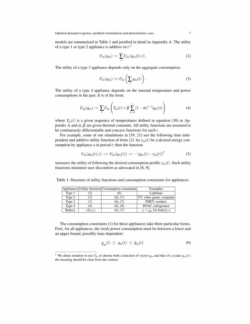
models are summarized in Table 1 and justified in detail in Appendix A. The utilityof a type 1 or type 2 appliance is additive in t:2
Uia(qia) := ∑t
Uia (qia(t), t) . (2)
The utility of a type 3 appliance depends only on the aggregate consumption:
Uia(qia) := Uia
(∑
tqia(t)
). (3)
The utility of a type 4 appliance depends on the internal temperature and powerconsumptions in the past. It is of the form:
Uiq(qia) := ∑t
Uia
(Tia(t)+β
t
∑τ=1
(1−α)t−τ qia(τ)
)(4)
where Tia(t) is a given sequence of temperatures defined in equation (30) in Ap-pendix A and α,β are given thermal constants. All utility functions are assumed tobe continuously differentiable and concave functions for each t.
For example, some of our simulations in [39, 21] use the following time inde-pendent and additive utility function of form (2): let yia(t) be a desired energy con-sumption by appliance a in period t; then the function
Uia(qia(t), t) := Uia(qia(t)) := −(qia(t)− yia(t))2 (5)
measures the utility of following the desired consumption profile yia(t). Such utilityfunctions minimize user discomfort as advocated in [8, 9].
Table 1: Structure of utility functions and consumption constraints for appliances.
Appliances Utility function Consumption constraints ExamplesType 1 (2) (6) LightingsType 2 (2) (6), (7) TV, video game, computerType 3 (3) (6), (7) PHEV, washersType 4 (4) (6), (8) HVAC, refrigeratorBattery −Di(ri) (6), (7) ri = qia for battery a
The consumption constraints (1) for these appliances take three particular forms.First, for all appliances, the (real) power consumption must lie between a lower andan upper bound, possibly time-dependent:
qia(t) ≤ qia(t) ≤ qia(t). (6)
2 We abuse notation to use Uia to denote both a function of vector qia and that of a scalar qia(t);the meaning should be clear from the context.

8 Lijun Chen, Na Li, Libin Jiang, and Steven H. Low
An important character of an appliance is its allowable time of operation; e.g., an EVcan be charged only between 9pm and 6am, TV may be on only between 7–9am and6–12pm. If an appliance operates only in a subset Tia ⊆ T of periods, we requirethat q
ia(t) = qia(t) = 0 for t 6∈ Tia and Uia(0) = 0. We therefore do not specify Tia
explicitly in the description of utility functions and always sum over all t ∈T . Thesecond kind of constraint specifies the range in which the aggregate consumptionmust lie:
Qia ≤ ∑t qia(t) ≤ Qia. (7)
The last kind of constraint is slightly more general (see derivation in Appendix A):
η ia ≤ Aiaqia ≤ η ia. (8)
Battery model. We denote by Bi the battery capacity, by bi(t) the state of charge inperiod t, and by ri(t) the power (energy per period) charged to (when ri(t) ≥ 0) ordischarged from (when ri(t)< 0) the battery in period t. We use a simplified modelof battery that ignores power leakage and other inefficiencies, where the state ofcharge is given by
bi(t) =t
∑τ=1
ri(τ)+bi(0). (9)
The battery has an upper bound on charge rate, denoted by ri, and an upper boundon discharge rate, denoted by −ri. We thus have the following constraints on bi(t)and ri(t):
0≤ bi(t)≤ Bi, ri ≤ ri(t)≤ ri. (10)
We assume any battery discharge is consumed by other appliances (zero leakage),and hence it cannot be more than what the appliances need:
−ri(t) ≤ ∑a∈Ai
qia(t). (11)
Finally, we impose a minimum on the energy level at the end of the control horizon:b(T )≥ γiBi where γi ∈ [0,1].
The cost of operating the battery is modeled by a function Di(ri) that depends onthe vector of charged/discharged power ri := (ri(t),∀t). This cost may correspondto the amortized purchase and maintenance cost of the battery over its lifetime, anddepends on how fast/much/often it is charged and discharged; see an example Di(ri)in [39]. The cost function Di is assumed to be a convex function of the vector ri.
Note that in this model, a battery is equivalent to an appliance: its utility functionis−Di(ri) and its consumption constraints (9), (10), and b(T )≥ γiBi are of the sameform as (6)–(7) with qia = ri. Therefore a battery can be specified simply as anotherappliance, in which case the constraint (11) requires that i’s aggregate demand benonnegative, ∑a∈Ai qia(t)+ ri(t) ≥ 0. This is summarized in Table 1. Henceforth,

Optimal demand response: problem formulation and deterministic case 9
we will often use appliances to also include battery and may not refer to batteryexplicitly when this does not cause confusion.
2.2 Supply model
We now describe a simple model of the electricity markets. The LSE procures powerfor delivery in each period t, in two steps. First it procures day-ahead capacities Pd(t)for each period t a day in advance and pays for the capacity costs cd(Pd(t); t). Therenewable power in each period t is a nonnegative random variable Pr(t) and it costscr(Pr(t); t). It is desirable to use as much renewable power as possible, for instance,if the renewable generation is owned by the LSE. For notational simplicity only, weassume cr(P; t) ≡ 0 for all P ≥ 0 and all t. Then at time t− (real time), the randomvariable Pr(t) is realized and used to satisfy demand. The LSE satisfies any excessdemand by some or all of the day-ahead capacity Pd(t) procured in advance and/orby purchasing balancing power on the real-time market. Let Po(t) denote the amountof the day-ahead power that the LSE actually uses and co(Po(t); t) its cost. Let Pb(t)be the real-time balancing power and cb(Pb(t); t) its cost.
These real-time decisions (Po(t),Pb(t)) are made by the LSE so as to minimizeits total cost, as follows. Given the demand vector q(t) := (qia(t),a ∈ Ai,∀i), letQ(t) := ∑i,a qia(t) be the total demand and ∆(Q(t)) := Q(t)−Pr(t) the excess de-mand, in excess of the renewable generation Pr(t). Note that ∆(Q(t)) is a randomvariable in and before period t− 1, but its realization is known to the LSE at timet−. Given excess demand ∆(Q(t)) and day-ahead capacity Pd(t), the LSE chooses(Po(t),Pb(t)) that minimizes its total real-time cost, i.e., it chooses (P∗o (t),P
∗b (t))
that solves the problem:
cs(∆(Q(t)),Pd(t); t) := minPo(t),Pb(t)
{ co(Po(t); t)+ cb(Pb(t); t) | Pb(t)≥ 0,
Po(t)+Pb(t)≥ ∆(Q(t)), Pd(t)≥ Po(t)≥ 0}. (12)
Clearly P∗o (t)+P∗b (t) = ∆(Q(t)) unless ∆(Q(t)< 0. The total cost is
c(Q(t),Pd(t);Pr(t), t) := cd(Pd(t); t)+ cs(∆(Q(t)),Pd(t); t). (13)
with ∆(Q(t)) := Q(t)−Pr(t). We assume that, for each t, cd(·; t), co(·; t) and cb(·; t)are increasing, convex, and continuously differentiable with cd(0; t) = co(0; t) =cb(0; t) = 0.
Example: supply costSuppose c′b(0)> c′o(P),∀P≥ 0, i.e., the marginal cost of balancing power is strictlyhigher than the marginal cost of day-ahead power, the LSE will use the balancingpower only after the day-ahead power is exhausted, i.e., Pb(t)> 0 only if ∆(Q(t))>Pd(t). The solution cs(∆(Q(t)),Pd(t); t) of (12) in this case is particularly simpleand (13) can be written explicitly in terms of cb,co,cb:

10 Lijun Chen, Na Li, Libin Jiang, and Steven H. Low
c(Q(t),Pd(t);Pr(t), t) = cd(Pd(t); t)+
co
([∆(Q(t))]Pd(t)
0 ; t)+ cb
([∆(Q(t))−Pd(t)]+ ; t
). (14)
i.e., the total cost consists of the capacity cost cd and the energy cost co of day-aheadpower, and the cost cb of the real-time balancing power. ut
2.3 Problem formulation: welfare maximization
Recall that q := (q(t), t ∈ T ) and Q(t) := ∑i,a qia(t). The social welfare is thestandard user utility minus supply cost:
W (q,Pd ;Pr) := ∑i,a
Uia(qia)−T
∑t=1
c(Q(t),Pd(t);Pr(t), t). (15)
As mentioned above the LSE’s objective is not to maximize its profit through sellingelectricity, but rather to maximize the expected social welfare. Given the day-aheaddecision Pd , the real-time procurement (Po(t),Pb(t)) is determined by the simpleoptimization (13). This is most transparent in (14) for the special case: the optimaldecision is to use day-ahead power P∗o (t) to satisfy any excess demand ∆(Q(t)) upto Pd(t), and then purchase real-time balancing power P∗b (t) = [∆(Q(t))−Pd(t)]+if necessary. Hence the maximization of (15) reduces to optimizing over day-aheadprocurement Pd and real-time consumption q in the presence of random renewablegeneration Pr(t). It is therefore critical that, in the presence of uncertainty, q(t)should be decided after Pr(t) have been realized at times t−. Pd however must bedecided a day ahead before Pr(t) are realized.
The traditional dynamic programming model requires that the objective functionbe separable in time t. The welfare function in (15) is not as the first term Uia(qia)depends on the entire control sequence qia = (qia(t),∀t). So does the consumptionconstraint (1). We now introduce an equivalent state space formulation of that willallow us to state precisely the overall optimization problem as an (1+ T )-perioddynamic program.
Consider a dynamical system over an extended time horizon t = 0,1, . . . ,T . Thecontrol inputs are the LSE’s day-ahead decision Pd := (Pd(t),∀t) in period 0 andthe user’s decisions q(t) in each subsequent period. Let v(t) denote the inputs, i.e.,v(0) = Pd and v(t) = q(t), t = 1, . . . ,T . Note that v(0) ∈ ℜT
+ whereas q(t) ∈ ℜM
where M :=∑Ni=1 |Ai|. The system state x(t) :=
(x1(t),x2
ia(t),x3(t),x4
ia(t), a ∈Ai,∀i)
has four components, defined as follows:
• Without loss of generality, x(0) starts from the origin.• x1(t) ∈ ℜT keeps track of the day-ahead decisions Pd : for each t = 1, . . . ,T ,
x1(t) = Pd = (Pd(τ),τ = 1, . . . ,T ).
Optimal demand response: problem formulation and deterministic case 11
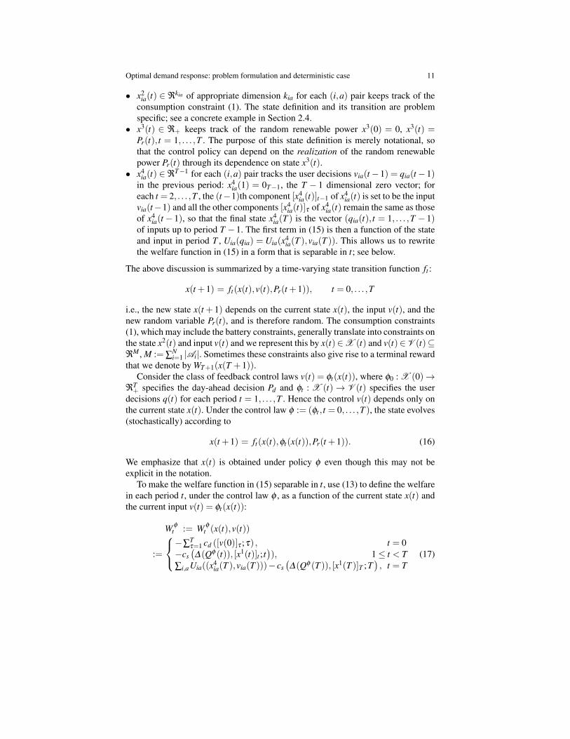
• x2ia(t) ∈ ℜkia of appropriate dimension kia for each (i,a) pair keeps track of the
consumption constraint (1). The state definition and its transition are problemspecific; see a concrete example in Section 2.4.
• x3(t) ∈ ℜ+ keeps track of the random renewable power x3(0) = 0, x3(t) =Pr(t), t = 1, . . . ,T . The purpose of this state definition is merely notational, sothat the control policy can depend on the realization of the random renewablepower Pr(t) through its dependence on state x3(t).
• x4ia(t) ∈ℜT−1 for each (i,a) pair tracks the user decisions via(t−1) = qia(t−1)
in the previous period: x4ia(1) = 0T−1, the T − 1 dimensional zero vector; for
each t = 2, . . . ,T , the (t−1)th component [x4ia(t)]t−1 of x4
ia(t) is set to be the inputvia(t−1) and all the other components [x4
ia(t)]τ of x4ia(t) remain the same as those
of x4ia(t− 1), so that the final state x4
ia(T ) is the vector (qia(t), t = 1, . . . ,T − 1)of inputs up to period T −1. The first term in (15) is then a function of the stateand input in period T , Uia(qia) = Uia(x4
ia(T ),via(T )). This allows us to rewritethe welfare function in (15) in a form that is separable in t; see below.
The above discussion is summarized by a time-varying state transition function ft :
x(t +1) = ft(x(t),v(t),Pr(t +1)), t = 0, . . . ,T
i.e., the new state x(t + 1) depends on the current state x(t), the input v(t), and thenew random variable Pr(t), and is therefore random. The consumption constraints(1), which may include the battery constraints, generally translate into constraints onthe state x2(t) and input v(t) and we represent this by x(t)∈X (t) and v(t)∈V (t)⊆ℜM , M := ∑
Ni=1 |Ai|. Sometimes these constraints also give rise to a terminal reward
that we denote by WT+1(x(T +1)).Consider the class of feedback control laws v(t) = φt(x(t)), where φ0 : X (0)→
ℜT+ specifies the day-ahead decision Pd and φt : X (t)→ V (t) specifies the user
decisions q(t) for each period t = 1, . . . ,T . Hence the control v(t) depends only onthe current state x(t). Under the control law φ := (φt , t = 0, . . . ,T ), the state evolves(stochastically) according to
x(t +1) = ft(x(t),φt(x(t)),Pr(t +1)). (16)
We emphasize that x(t) is obtained under policy φ even though this may not beexplicit in the notation.
To make the welfare function in (15) separable in t, use (13) to define the welfarein each period t, under the control law φ , as a function of the current state x(t) andthe current input v(t) = φt(x(t)):
W φ
t := W φ
t (x(t),v(t))
:=
−∑Tτ=1 cd ([v(0)]τ ;τ) , t = 0
−cs(∆(Qφ (t)), [x1(t)]t ; t
)), 1≤ t < T
∑i,a Uia((x4ia(T ),via(T )))− cs
(∆(Qφ (T )), [x1(T )]T ;T
), t = T
(17)

12 Lijun Chen, Na Li, Libin Jiang, and Steven H. Low
where Qφ (t) =∑i,a[v(t)]ia is the aggregate demand in period t under φ , and via(T ) =qia(T ) are the real-time consumption decisions in the last control period T . Then thewelfare function in (15) is equivalent to
Jφ :=T
∑t=0
W φ
t (x(t),v(t))+W φ
T+1(x(T +1))
where the definition of the terminal reward W φ
T+1(x(T + 1)) is problem specific.We can now state precisely our objective as the constrained maximization of theexpected welfare over the control law φ :
maxφ
E Jφ = E
(T
∑t=0
W φ
t +W φ
T+1
)s. t. xφ (t) ∈X (t). (18)
where the expectation is taken over Pr(t), t = 1, . . . ,T .
Remark. An important assumption in this formulation is that the consumption con-straints (1) can be modeled by an appropriate definition of states x2
ia(t), their transi-tions ft , the constraint sets X (t),V (t), and possibly a terminal reward WT+1(x(T +1)).
We now illustrate the problem formulation using a concrete example.
2.4 Example
To simplify the notation we make two assumptions that do not cause any loss ofgenerality. First we use the total cost function c in (14) in the definition of the welfarefunction (15). Second we assume each user i has a single type-2 appliance and nobattery (so we drop the subscript a). From Table 1, user utility functions are additivein time, Ui(qi) = ∑t Ui(qi(t); t) and the consumption constraints are
qi(t) ≤ qi(t) ≤ qi(t), ∀i (19)
Qi ≤ ∑Tt=1 qi(t). (20)
Since the utility functions are separable in t, we do not need to define x4(t). We nowdescribe the (1+T )-period dynamic program by specifying the definition of x2(t),the state transition function ft , and the constraint sets X (t),V (t).
The system state x(t) := (x1(t),x2(t),x3(t)) consists of three components of ap-propriate dimensions with
x(t) = (Pd ,x2(t),Pr(t)), t = 1, . . . ,T
where x2(t) is determined by the constraint (20). To simplify exposition, we makethe important assumption that Pr(t) are independent for different t; see [21] for
Optimal demand response: problem formulation and deterministic case 13
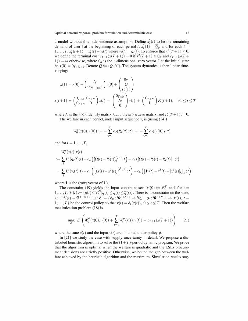
a model without this independence assumption. Define x2i (t) to be the remaining
demand of user i at the beginning of each period t: x2i (1) = Qi, and for each t =
1, . . . ,T , x2i (t +1) = x2
i (t)−vi(t) where vi(t) = qi(t). To enforce that x2(T +1)≤ 0,we define the terminal cost cT+1(x(T +1)) = 0 if x2(T +1) ≤ 0N and cT+1(x(T +1)) = ∞ otherwise, where 0n is the n-dimensional zero vector. Let the initial statebe x(0) = 0T+N+1. Denote Q := (Qi,∀i). The system dynamics is then linear time-varying:
x(1) = x(0)+(
IT0(N+1)×T
)v(0)+
0TQ
Pr(1)
x(t +1) =
(IT+N 0T+N0T+N 0
)x(t) −
0T×NIN0
v(t) +
(0T+N
1
)Pr(t +1), ∀1≤ t ≤ T
where In is the n×n identify matrix, 0m×n the m×n zero matrix, and Pr(T +1) := 0.The welfare in each period, under input sequence v, is (using (14))
W v0 (x(0),v(0)) := −
T
∑τ=1
cd(Pd(τ);τ) = −T
∑τ=1
cd([v(0)]τ ;τ)
and for t = 1, . . . ,T ,
W vt (x(t),v(t))
:= ∑i
Ui(qi(t); t)− co
([Q(t)−Pr(t)]
Pd(t)0 ; t
)− cb
([Q(t)−Pr(t)−Pd(t)]+ ; t
)= ∑
iUi(vi(t); t)− co
([1v(t)− x3(t)
][x1(t)]t0 ; t
)− cb
([1v(t)− x3(t)− [x1(t)]t
]+
; t)
where 1 is the (row) vector of 1’s.The constraint (19) yields the input constraint sets V (0) := ℜT
+ and, for t =1, . . . ,T , V (t) := {q(t)∈ℜN |q(t)≤ q(t)≤ q(t)}. There is no constraint on the state,i.e., X (t) = ℜT+N+1. Let φ := {φ0 : ℜT+N+1 → ℜT
+, φt : ℜT+N+1 → V (t), t =1, . . . ,T} be the control policy so that v(t) = φt(x(t)), 0 ≤ t ≤ T . Then the welfaremaximization problem (18) is
maxφ
E
(W φ
0 (x(0),v(0)) +T
∑t=1
W φ
t (x(t),v(t)) − cT+1 (x(T +1))
)(21)
where the state x(t) and the input v(t) are obtained under policy φ .In [21] we study the case with supply uncertainty in detail. We propose a dis-
tributed heuristic algorithm to solve the (1+T )-period dynamic program. We provethat the algorithm is optimal when the welfare is quadratic and the LSEs procure-ment decisions are strictly positive. Otherwise, we bound the gap between the wel-fare achieved by the heuristic algorithm and the maximum. Simulation results sug-

14 Lijun Chen, Na Li, Libin Jiang, and Steven H. Low
gest that the performance of the heuristic algorithm is very close to optimal. As wescale up the size of a renewable generation plant, both its mean production and itsvariance will likely increase. As expected, the maximum welfare increases with themean production, when the variance is fixed, and decreases with the variance, whenthe mean is fixed. More interesting, we prove that as we scale the size of the plantup, the maximum welfare increases.
3 Optimal scheduling without supply uncertainty
In this paper we only fully treat the case where there is no supply uncertainty, i.e.,Pr(t)≡ 0. Our goal is to optimally coordinate supply and demand to maximize socialwelfare. In the absence of uncertainty (our model also ignores demand uncertainty),it becomes unnecessary to adapt user consumptions in real-time and hence supplyand consumptions can be optimally scheduled at once instead of over two days.Welfare maximization (18) then takes a simpler form and we develop an offlinedistributed algorithm that jointly optimizes the LSE’s procurements and the users’consumptions for each period in the following day.
3.1 Optimal procurements and consumptions
We first consider LSE’s procurement decisions. Recall that Qi(t) := ∑a∈Ai qia(t)and ∑i Qi(t) is the aggregate demand in period t. With supply uncertainty, while Pdis decided a day ahead, the optimization (12) must be carried out in real time afterPr(t) has been realized to obtain optimal Po(t),Pb(t). Here, on the other hand, allthree decisions (Pd(t),Po(t),Pb(t)) can be computed in advance in the absence ofuncertainty. Hence, given an aggregate demand ∑i Qi(t), the LSE solves (instead of(12)–(13)):
c
(∑
iQi(t); t
):= min
Pd(t),Po(t),Pb(t)cd(Pd(t); t)+ co(Po(t); t)+ cb(Pb(t); t) (22)
s. t. Po(t)+Pb(t)≥∑i
Qi(t), Pd(t)≥ Po(t)≥ 0, Pb(t)≥ 0
to obtain the total cost. The solution of (22) specifies the optimal decisions (P∗d (t),P∗o (t),P
∗b (t))
to satisfy the aggregate demand ∑i Qi(t) for each period t in the following day.It is not difficult to show that c(·, t) is an non-decreasing, convex, and con-
tinuously differentiable function for each t, so the problem (22) is convex. Sincec′d(P; t) > 0, the KKT condition implies that P∗d (t) = P∗o (t) at optimality, i.e., itis optimal to exhaust all the day-ahead capacity. This is always possible becauseall procurement decisions are computed jointly without uncertainty. If we furtherassume that the marginal cost of the balancing power is higher than that of the day-

Optimal demand response: problem formulation and deterministic case 15
ahead power, i.e., c′b(0; t)> c′d(P; t)+ c′o(P; t) for all P≥ 0, then KKT implies thatit will never pay to use balancing power, i.e., P∗b (t) = 0 at optimality. In this case,P∗d (t) = P∗o (t) = ∑i Qi(t).
Hence welfare maximization reduces to the computation of the user consump-tions qia(t); the corresponding procurement decisions are then given by (22). Theoptimization of the social welfare in (15) then becomes:
maxq ∑
i,aUia(qia)−∑
tc
(∑
iQi(t); t
)(23)
s. t. Aiaqia ≤ ηia, a ∈Ai,∀i, (24)0 ≤ Qi(t) ≤ Qi, ∀i (25)
The inequalities in (24) are the consumption constraints (1) of user i’s appliancesand battery. The lower inequality in (25) is the same as (11); see the discussion atthe end of Section 2.1 on battery constraints. The upper inequality in (25) imposesa bound on the total power drawn by user i. By assumption, the objective functionis concave and the feasible set is convex. Hence an optimal point can in principlebe computed offline centrally by the LSE. This however will require that the LSEknow all the users’ utility and battery cost functions and all the constraints, whichis impractical for technical or privacy reasons. The goal of this section is to derive adistributed algorithm to solve (23)–(25) by decomposing it into subproblems that aresolvable in a decentralized manner where the LSE only needs to know the aggregatedemand but not the individual private information.
The key idea is for the LSE to set prices π := (π(t),∀t) to induce the users toindividually choose socially optimal consumptions qi := (qia(t),∀t) in response.Indeed, given prices π , we assume that each user i chooses its own demand qi so asto maximize its net benefit, her total utility minus the electricity cost, i.e., each useri solves:
maxqi
∑a∈Ai
Uia(qia)−∑t
π(t)Qi(t) s. t. (24)− (25). (26)
Given prices π , we denote an individually optimal solution of (26) and the corre-sponding aggregate demand by
qi(π) := (qia(t;π),∀t,∀a ∈Ai), Qi(π) := (Qi(t;π), ∀t) :=
(∑
a∈Ai
qi,a(t;π),∀t
).
Recall q(π) := (qi(π), ∀i). It is a remarkable fact in the competitive equilibriumtheory in economics that there exist prices π that align the individual optimalitywith the social optimality, i.e., there are prices π∗ such that if qi(π
∗) optimize i’sobjectives for all users i then they also optimize the social welfare.
16 Lijun Chen, Na Li, Libin Jiang, and Steven H. Low
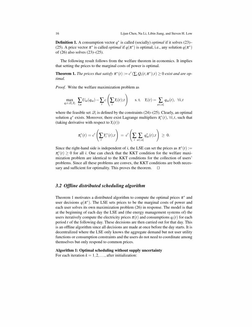
Definition 1. A consumption vector q∗ is called (socially) optimal if it solves (23)–(25). A price vector π∗ is called optimal if q(π∗) is optimal, i.e., any solution q(π∗)of (26) also solves (23)–(25).
The following result follows from the welfare theorem in economics. It impliesthat setting the prices to the marginal costs of power is optimal.
Theorem 1. The prices that satisfy π∗(t) := c′ (∑i Qi(t;π∗); t)≥ 0 exist and are op-timal.
Proof. Write the welfare maximization problem as
maxqi∈Qi,Yi
∑i,a
Uia(qia)−∑t
c
(∑
iYi(t); t
)s. t. Yi(t) = ∑
a∈Ai
qia(t), ∀i, t
where the feasible set Qi is defined by the constraints (24)–(25). Clearly, an optimalsolution q∗ exists. Moreover, there exist Lagrange multipliers π∗i (t), ∀i, t, such that(taking derivative with respect to Yi(t))
π∗i (t) = c′
(∑
iY ∗i (t); t
)= c′
(∑
i∑
a∈Ai
q∗ia(t); t
)≥ 0.
Since the right-hand side is independent of i, the LSE can set the prices as π∗(t) :=π∗i (t) ≥ 0 for all i. One can check that the KKT condition for the welfare maxi-mization problem are identical to the KKT conditions for the collection of users’problems. Since all these problems are convex, the KKT conditions are both neces-sary and sufficient for optimality. This proves the theorem. ut
3.2 Offline distributed scheduling algorithm
Theorem 1 motivates a distributed algorithm to compute the optimal prices π∗ anduser decisions q(π∗). The LSE sets prices to be the marginal costs of power andeach user solves its own maximization problem (26) in response. The model is thatat the beginning of each day the LSE and (the energy management systems of) theusers iteratively compute the electricity prices π(t) and consumptions qi(t) for eachperiod t of the following day. These decisions are then carried out for that day. Thisis an offline algorithm since all decisions are made at once before the day starts. It isdecentralized where the LSE only knows the aggregate demand but not user utilityfunctions or consumption constraints and the users do not need to coordinate amongthemselves but only respond to common prices.
Algorithm 1: Optimal scheduling without supply uncertaintyFor each iteration k = 1,2, . . . , after initialization:
Optimal demand response: problem formulation and deterministic case 17
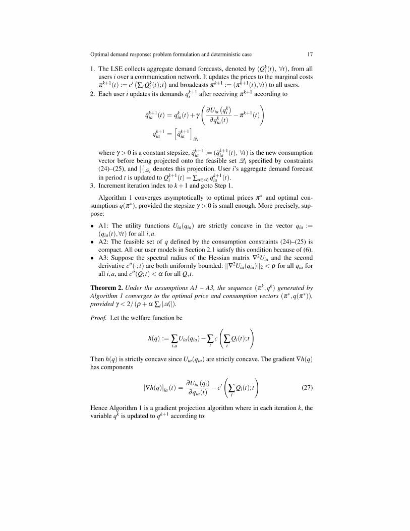
1. The LSE collects aggregate demand forecasts, denoted by (Qki (t), ∀t), from all
users i over a communication network. It updates the prices to the marginal costsπk+1(t) := c′
(∑i Qk
i (t); t)
and broadcasts πk+1 := (πk+1(t),∀t) to all users.2. Each user i updates its demands qk+1
i after receiving πk+1 according to
qk+1ia (t) = qk
ia(t)+ γ
(∂Uia
(qk
i)
∂qkia(t)
−πk+1(t)
)qk+1
ia =[qk+1
ia
]Qi
where γ > 0 is a constant stepsize, qk+1ia := (qk+1
ia (t), ∀t) is the new consumptionvector before being projected onto the feasible set Qi specified by constraints(24)–(25), and [·]Qi denotes this projection. User i’s aggregate demand forecastin period t is updated to Qk+1
i (t) = ∑a∈Ai qk+1ia (t).
3. Increment iteration index to k+1 and goto Step 1.
Algorithm 1 converges asymptotically to optimal prices π∗ and optimal con-sumptions q(π∗), provided the stepsize γ > 0 is small enough. More precisely, sup-pose:
• A1: The utility functions Uia(qia) are strictly concave in the vector qia :=(qia(t),∀t) for all i,a.
• A2: The feasible set of q defined by the consumption constraints (24)–(25) iscompact. All our user models in Section 2.1 satisfy this condition because of (6).
• A3: Suppose the spectral radius of the Hessian matrix ∇2Uia and the secondderivative c′′(·; t) are both uniformly bounded: ‖∇2Uia(qia)‖2 < ρ for all qia forall i,a, and c′′(Q; t)< α for all Q, t.
Theorem 2. Under the assumptions A1 – A3, the sequence (πk,qk) generated byAlgorithm 1 converges to the optimal price and consumption vectors (π∗,q(π∗)),provided γ < 2/(ρ +α ∑i |Ai|).
Proof. Let the welfare function be
h(q) := ∑i,a
Uia(qia)−∑t
c
(∑
iQi(t); t
)
Then h(q) is strictly concave since Uia(qia) are strictly concave. The gradient ∇h(q)has components
[∇h(q)]ia (t) =∂Uia (qi)
∂qia(t)− c′
(∑
iQi(t); t
)(27)
Hence Algorithm 1 is a gradient projection algorithm where in each iteration k, thevariable qk is updated to qk+1 according to:

18 Lijun Chen, Na Li, Libin Jiang, and Steven H. Low
qk+1 =[qk + γ∇h(qk)
]Q
where Q :=Q1×·· ·×QN . Moreover assumption A3 implies the following lemma,proved in Appendix B.
Lemma 1. ∇h(q) is Lipschitz with ‖∇h(q)−∇h(q)‖2 < (ρ +α ∑i |Ai|)‖q− q‖2 forall q, q.
Lemma 1 implies that, provided γ < 2/(ρ +α ∑i |Ai|), any accumulation point q∗
of the sequence qk generated by Algorithm 1 is optimal, i.e., maximizes welfareh(q) [40, p. 214]. Assumption A2 implies that the sequence qk lies in a compactset and hence must have a convergent subsequence. But assumption A1 impliesthat the optimal q∗ is unique. Therefore all convergent subsequences, hence theoriginal sequence qk, must converge to q∗. By continuity of c′, πk(t)= c′(∑i Qk
i (t); t)converges to the unique price c′(∑i Q∗i (t); t) with Q∗i (t) := ∑a∈Ai q∗ia(t) which, byTheorem 1, is optimal. ut
The rate of convergence of Algorithm 1 depends on the stepsize γ: a larger γ gen-erally leads to faster convergence, but a large γ can also risk instability. The boundon the stepsize γ in Theorem 2 is conservative; in practice a much larger stepsizecan usually be used without losing stability. We simulate this algorithm in [39] withrealistic system parameters. The simulation results show that, as expected, the pricesare capable of coordinating the decisions of different appliances in a decentralizedmanner, to reduce peak aggregate demand and flatten its profile, greatly increasingthe load factor. Furthermore, battery amplifies the benefits of demand response.
4 Conclusion
We have presented a simple yet versatile user model and formulated the optimaldemand response problem as an (1+T )-period dynamic program to maximize theexpected social welfare. In this paper, we have focused on the case where thereis no uncertainty. In this case demand response reduces to the deterministic welfaremaximization in (23)–(25) that has a natural decentralized and incentive-compatiblestructure. We have proposed an offline distributed scheduling algorithm where theLSE sets the day-ahead prices to be their marginal costs based on forecast demandsand, in response, the users forecast their demands to maximize their own surplus.As long as the stepsize is small enough, this procedure will converge to the uniqueoptimal prices and consumptions. The algorithm is decentralized where the LSEonly knows the aggregate demand but not user utility functions or consumptionconstraints, and the users do not need to coordinate with other users but only respondto the common prices from the LSE.
The current work has several limitations. First our model does not include thedistribution system, implicitly assuming that the underlying network has enoughcapacity to distribute the power demanded by the users without causing congestion.

Optimal demand response: problem formulation and deterministic case 19
Second we only consider power balance in steady-state and ignore fast timescaledynamics such as frequency and voltage fluctuations due to random supply and de-mand. Third we do not model power market dynamics; for example, our modelassumes that the cost functions faced by the LSE are independent of the demandsand we ignore economic issues such as revenue-adequacy for the LSE. Finally ourresults are only for the case without uncertainty. When there is random renewablegeneration, offline scheduling alone will be insufficient and real-time demand re-sponse should be employed to match fluctuating spply. This is considered in [21].
Appendix A: Detailed appliance models
We describe detailed models of common electric appliances summarized in Section2.1.
Type 1. This category of appliances includes lighting that must be on for a cer-tain period of time. The consumption constraint is (6), with the understanding thatq
ia(t) = qia(t) = 0 for periods t that are outside its time of operation. User i attains
a utility Uia(qia(t), t) from consuming power qia(t) independent of its consumptionin other periods, and the overall utility (2) is therefore separable in t.
Type 2. This category includes TV, video games, and computers. For these appli-ances, a user’s utility depends on her consumption in each period she wishes to useit as well as the total amount of consumption in a day. Hence the consumption con-straints are (6) and (7). For example, a user may have a favorite TV program thatshe wishes to watch everyday. With DVR, she can watch the program at any time.However the total power demand of TV should at least cover the program. Type 2appliances have the same kind of utility functions (2) as Type 1 appliances. The timedependent utility function models the fact that a user may get different benefits fromconsuming the same amount of power at different times, e.g., she may enjoy a TVprogram to different levels at different times.
Type 3. This category includes PHEV, dish washer, clothes washer. For these ap-pliances, a user only cares about whether the task is completed by a certain time.This means that the aggregate power consumption by such an appliance must ex-ceed a threshold within its time of operation [28, 29, 33]. Hence the consumptionconstraints are (6) and (7). The utility depends only on the total power consumed,hence (3).
Type 4. This category includes HVAC (heating, ventilation, air conditioning) andrefrigerator that control the temperature of a user’s environment. Let T in
ia (t) andT out
ia (t) denote the temperatures at time t inside and outside the place that appliance(i,a) is in charge of, and Tia denotes the set of times when user i cares about thetemperature. For instance, for air conditioner, T in
ia (t) is the temperature inside thehouse, T out
ia (t) is the temperature outside the house, and Tia is the set of times whenshe is at home.

20 Lijun Chen, Na Li, Libin Jiang, and Steven H. Low
The inside temperature evolves according to the following linear dynamics [27,9, 26]:
T inia (t) = T in
ia (t−1)+α(T outia (t)−T in
ia (t−1))+βqia(t) (28)
where α and β are parameters that specify thermal characteristics of the applianceand the environment in which it operates. The second term in equation (28) modelsheat transfer. The third term models the thermal efficiency of the system; β > 0 ifappliance a is a heater and β < 0 if it is a cooler. Here, we define T in
ia (0) as thetemperature T in
ia (T ) from the previous day. Let [T ia, T ia] be a range of preferredtemperature, leading to the constraint:
T ia ≤ T inia (t) ≤ T ia, ∀t ∈Tia. (29)
Using Equation (28), we can write T inia (t) in terms of (qia(τ),τ = 1, . . . , t):
T inia (t) = (1−α)tT in
ia (0)+t
∑τ=1
(1−α)t−ταT out
ia (τ)+β
t
∑τ=1
(1−α)t−τ qia(τ).
Define
Tia(t) := (1−α)tT inia (0)+
t
∑τ=1
(1−α)t−ταT out
ia (τ). (30)
Then
T inia (t) = Tia(t)+β
t
∑τ=1
(1−α)t−τ qia(τ). (31)
With (31), the constraint (29) becomes a linear constraint on the load vector qia: forany t ∈Tia,
T ia ≤ Tia(t)+β
t
∑τ=1
(1−α)t−τ qia(τ)≤ T ia.
This is the constraint (8), in addition to (6). Assume user i attains a utility Uia(T inia (t))
when the temperature is T ini,a(t). Then (31) gives the utility function (4).
Appendix B: Proof of Lemma 1
We first describe the Hessian ∇2h(q). Let N := |N | be the number of users and A :=|∪i∈N Ai| the total number of appliances. Let k take value (i,a) for i = 1, . . . ,N,a =1, . . . ,A. For k = (i,a), let 1k be 1 if a ∈ Ai and 0 otherwise. From (27), ∇2h(q) isgiven by
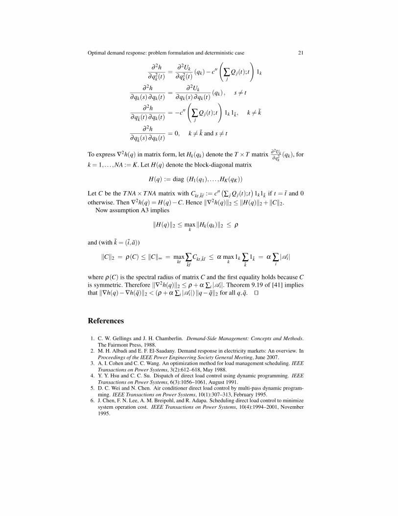
Optimal demand response: problem formulation and deterministic case 21
∂ 2h∂q2
k(t)=
∂ 2Uk
∂q2k(t)
(qk)− c′′(
∑j
Q j(t); t
)1k
∂ 2h∂qk(s)∂qk(t)
=∂ 2Uk
∂qk(s)∂qk(t)(qk) , s 6= t
∂ 2h∂qk(t)∂qk(t)
= −c′′(
∑j
Q j(t); t
)1k 1k, k 6= k
∂ 2h∂qk(s)∂qk(t)
= 0, k 6= k and s 6= t
To express ∇2h(q) in matrix form, let Hk(qk) denote the T ×T matrix ∂ 2Uk∂q2
k(qk), for
k = 1, . . . ,NA := K. Let H(q) denote the block-diagonal matrix
H(q) := diag (H1(q1), . . . ,HK(qK))
Let C be the T NA× T NA matrix with Ckt,kt := c′′(∑ j Q j(t); t
)1k1k if t = t and 0
otherwise. Then ∇2h(q) = H(q)−C. Hence ‖∇2h(q)‖2 ≤ ‖H(q)‖2 +‖C‖2.Now assumption A3 implies
‖H(q)‖2 ≤ maxk‖Hk(qk)‖2 ≤ ρ
and (with k = (i, a))
‖C‖2 = ρ(C) ≤ ‖C‖∞ = maxkt
∑kt
Ckt,kt ≤ α maxk
1k ∑k
1k = α ∑i|Ai|
where ρ(C) is the spectral radius of matrix C and the first equality holds because Cis symmetric. Therefore ‖∇2h(q)‖2 ≤ ρ +α ∑i |Ai|. Theorem 9.19 of [41] impliesthat ‖∇h(q)−∇h(q)‖2 < (ρ +α ∑i |Ai|)‖q− q‖2 for all q, q. ut
References
1. C. W. Gellings and J. H. Chamberlin. Demand-Side Management: Concepts and Methods.The Fairmont Press, 1988.
2. M. H. Albadi and E. F. El-Saadany. Demand response in electricity markets: An overview. InProceedings of the IEEE Power Engineering Society General Meeting, June 2007.
3. A. I. Cohen and C. C. Wang. An optimization method for load management scheduling. IEEETransactions on Power Systems, 3(2):612–618, May 1988.
4. Y. Y. Hsu and C. C. Su. Dispatch of direct load control using dynamic programming. IEEETransactions on Power Systems, 6(3):1056–1061, August 1991.
5. D. C. Wei and N. Chen. Air conditioner direct load control by multi-pass dynamic program-ming. IEEE Transactions on Power Systems, 10(1):307–313, February 1995.
6. J. Chen, F. N. Lee, A. M. Breipohl, and R. Adapa. Scheduling direct load control to minimizesystem operation cost. IEEE Transactions on Power Systems, 10(4):1994–2001, November1995.

22 Lijun Chen, Na Li, Libin Jiang, and Steven H. Low
7. K. H. Ng and G. B. Sheble. Direct load control – a profit-based load management using linearprogramming. IEEE Transactions on Power Systems, 13(2):688–695, May 1998.
8. W.-C. Chu, B.-K. Chen, and C.-K. Fu. Scheduling of direct load control to minimize load re-duction for a utility suffering from generation shortage. IEEE Transactions on Power Systems,8(4):1525–1530, November 1993.
9. B. Ramanathan and V. Vittal. A framework for evaluation of advanced direct load control withminimum disruption. IEEE Transactions on Power Systems, 23(4):1681–1688, November2008.
10. M. D. Ilic, L. Xie, and J.-Y. Joo. Efficient coordination of wind power and price-responsivedemand part I: Theoretical foundations; part II: Case studies. IEEE Transactions on PowerSystems, 99, 2011.
11. Y. V. Makarov, C. Loutan, J. Ma, and P. de Mello. Operational impacts of wind generationon California power systems. IEEE Transactions on Power Systems, 24(2):1039–1050, May2009.
12. M. C. Caramanis and J. M. Foster. Coupling of day ahead and real-time power markets forenergy and reserves incorporating local distribution network costs and congestion. In Pro-ceedings of the 48th Annual Allerton Conference, September – October 2010.
13. D. Kirschen. Demand-side view of electricity market. IEEE Transactions on Power Systems,18(2):520–527, May 2003.
14. J. C. Smith, M. R. Milligan, E. A. DeMeo, and B. Parsons. Utility wind integration andoperating impact: State of the art. IEEE Transactions on Power Systems, 22(3):900–908,August 2007.
15. N. Ruiz, I. Cobelo, and J. Oyarzabal. A direct load control model for virtual power plantmanagement. IEEE Transactions on Power Systems, 24(2):959–966, May 2009.
16. P. P. Varaiya, F. F. Wu, and J. W. Bialek. Smart operation of smart grid: Risk-limiting dispatch.Proceedings of the IEEE, 99(1):40 –57, January 2011.
17. Department of Energy. Benefits of demand response in electricity markets and recommenda-tions for achieving them. Technical report, February 2006.
18. S. Borenstein. Time-varying retail electricity prices: Theory and practice. In Griffin and Puller,editors, Electricity Deregulation: Choices and Challenges. University of Chicago Press, 2005.
19. C. Triki and A. Violi. Dynamic pricing of electricity in retail markets. Quarterly Journal ofOperations Research, 7(1):21–36, March 2009.
20. M. D. Ilic. Dynamic monitoring and decision systems for enabling sustainable energy services.Proceedings of the IEEE, 99(1):58–79, January 2011.
21. L. Jiang and S. H. Low. Optimal demand response: with uncertain supply. In Technical Report,2011.
22. P. M. Schwarz, T. N. Taylor, M. Birmingham, and S. L. Dardan. Industrial response to elec-tricity real-time prices: Short run and long run. Economic Inquiry, 40(4):597–610, 2002.
23. C. Goldman, N. Hopper, R. Bharvirkar, B. Neenan, R. Boisvert, P. Cappers, D. Pratt, andK. Butkins. Customer strategies for responding to day-ahead market hourly electricity pricing.Technical report, Lawrence Berkeley National Lab, LBNL-57128, August 2005. Report forCA Energy Commission.
24. T. N. Taylor, P. M. Schwarz, and J. E. Cochell. 24-7 hourly response to real-time pricing withup to eight summers of experience. Journal of Regulatory Economics, 27(3):235–262, January2005.
25. S. Borenstein. The long-run efficiency of real-time electricity pricing. The Energy Journal,26(3):93–116, Febuary 2005.
26. J.E. Braun. Load control using building thermal mass. Journal of solar energy engineering,125(3):292–301, August 2003.
27. P. Xu, P. Haves, M. A. Piette, and L. Zagreus. Demand shifting with thermal mass in largecommercial buildings: Field tests, simulation and audits. Technical report, Lawrence BerkeleyNational Lab, LBNL-58815, 2006.
28. A. Mohsenian-Rad and A. Leon-Garcia. Optimal residential load control with price predictionin real-time electricity pricing environments. IEEE Transactions on Smart Grid, 1(2):120–133, September 2010.
Optimal demand response: problem formulation and deterministic case 23
29. M. Pedrasa, T. Spooner, and I. MacGill. Coordinated scheduling of residential distributedenergy resources to optimize smart home energy services. IEEE Transactions on Smart Grid,1(2):134–143, September 2010.
30. S. Caron and G. Kesidis. Incentive-based energy consumption scheduling algorithms for thesmart grid. In Proceedings of the IEEE International Conference on Smart Grid Communica-tions, October 2010.
31. M. C. Caramanis and J. M. Foster. Management of electric vehicle charging to mitigate re-newable generation intermittency and distribution network congestion. In Proceedings of the48th IEEE Conference on Decision and Control (CDC), December 2009.
32. Z. Ma, D. Callaway, and I. Hiskens. Decentralized charging control for large populationsof plug-in electric vehicles. In Proceedings of the 49th IEEE Conference on Decision andControl (CDC), December 2010.
33. K. Clement-Nyns, E. Haesen, and J. Driesen. The impact of charging plug-in hybrid electricvehicles on a residential distribution grid. IEEE Transactions on Power Systems, 25(1):371–380, Febuary 2010.
34. L. Chen, N. Li, and S.H. Low. Two Market Models for Demand Response in Power Net-works. In Proceedings of the IEEE International Conference on Smart Grid Communications,October 2010.
35. G. Pritchard, G. Zakeri, and A. Philpott. A single-settlement, energy-only electric powermarket for unpredictable and intermittent participants. Operations Research, 58(4):1210–1219, July-August 2010.
36. M. J. Neely, A. S. Tehrani, and A. G. Dimakis. Efficient algorithms for renewable energyallocation to delay tolerant consumers. In Proceedings of the IEEE International Conferenceon Smart Grid Communications, October 2010.
37. Miao He, Sugumar Murugesan, and Junshan Zhang. Multiple timescale dispatch and schedul-ing for stochastic reliability in smart grids with wind generation integration. preprint, CoRR,abs/1008.3932, 2010.
38. C.-W. Tan and P. P. Varaiya. Interruptible electric power service contracts. Journal of Eco-nomic Dynamics and Control, 17(3):495–517, May 1993.
39. N. Li, L. Chen, and S. H. Low. Optimal Demand Response Based on Utility Maximization inPower Networks. In Proceedings of IEEE Power Engineering Society General Meeting, July2011.
40. D. P. Bertsekas and J. N. Tsitsiklis. Parallel and distributed computation. Old Tappan, NJ(USA); Prentice Hall Inc., 1989.
41. W. Rudin. Principles of Mathematical Analysis. McGraw-Hill Inc., 3 edition, 1976.