optimal control techniques for management strategies in ... · caicó canguaretama ceará mirim...
TRANSCRIPT

Optimal control techniques for managementstrategies in biological models
Suzanne Lenhart
University of Tennessee, Knoxville
June 2, 2018
Lenhart (UTK) Management Strategies June 2, 2018 1 / 52

Outline
1. First Part: Formulation of PDE model for Zika virus in Brazil
2. Discussion of data, parameter estimation and numerical results
3. Second Part: Management of Fire Model
Lenhart (UTK) Management Strategies June 2, 2018 2 / 52

First Part
Optimal control of vaccination in a vector-bornereaction-diffusion model applied to Zika virus -Preliminary Report
collaborators: T. Miyaoka, J. MeyerU of Campinas - Brazil
Lenhart (UTK) Management Strategies June 2, 2018 3 / 52

Modeling Zika Virus in Brazil
Zika Virus is a Flavivirus and is primarily transmitted to humansmainly by Aedes aegypti mosquitoesZika can also be transmitted by vertical transmisson, sexualrelations and blood transfusions.Zika virus: concern about children born with neurologicalconditions (microcephaly)Vaccines still in development (clinical trial)How to balance the cost benefit in vaccination?
Goal: Apply optimal control of vaccination in a partial differentialequation model using data in a state in Brazil .
Lenhart (UTK) Management Strategies June 2, 2018 4 / 52
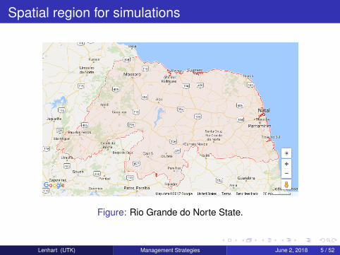
Spatial region for simulations
Figure: Rio Grande do Norte State.
Lenhart (UTK) Management Strategies June 2, 2018 5 / 52

Mathematical modeling
Reaction–Diffusion PDE model.
SIR dynamics for humans and SI for mosquitoes.S, I,R susceptible, infected, recovered (vaccinated) for humansSv, Iv susceptible, infected for mosquitoes
Vaccination rate u gives immunity to susceptible humans.
Control using the vaccination rate u(x, t).
Lenhart (UTK) Management Strategies June 2, 2018 6 / 52
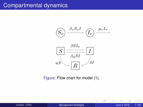
Compartmental dynamics
S I
R
Sv Iv
uS
βSIv
βdSI
βvSvI µvIv
δI
Figure: Flow chart for model (1).
Lenhart (UTK) Management Strategies June 2, 2018 7 / 52

Model in Weak solution sense
∂S
∂t−∇ · (α∇S) = −βSIv − βdSI − uS,
∂I
∂t−∇ · (αI∇I) = βSIv + βdSI − δI,
∂R
∂t−∇ · (α∇R) = uS + δI,
∂Sv∂t−∇ · (αv∇Sv) = −βvSvI + rv (Sv + Iv)
(1− (Sv + Iv)
κv
),
∂Iv∂t−∇ · (αv∇Iv) = βvSvI − µvI, in Q = Ω× (0, T ).
(1)
Plus initial conditions and no flux boundary conditions.Logistic growth for mosquitoesIn the simulations, sexual transmission coefficient was estimatedto be 0.
Lenhart (UTK) Management Strategies June 2, 2018 8 / 52

Optimal control
Goal: minimize cost of infecteds and administering the vaccinecontrol:
J(u) =
∫Q
(c1I(x, t) + c2u(x, t)S(x, t) + c3u(x, t)2)dxdt.
The control setu ∈ L2(Q), 0 ≤ u ≤ umax
Lenhart (UTK) Management Strategies June 2, 2018 9 / 52

Necesary Condtions for Optimal control
To derive necessary conditions for an optimal control, we need todifferentiate the map u→ J(u)
Since J(u) depends on the states, we must differentiate the map,u→ S, I,R, Sv, IvUsing sensitivities (derivatives of states with respect to control),we derive an adjoint PDE system:
L∗(λ) +MTλ = (c2u, c1, 0, 0, 0)T ,
MT =
βIv + βdI + u −βIv − βdI −u 0 0
βdS δ − βdS −δ βvSv −βvSv0 0 0 0 0
0 0 0 −rv +2rvκv
(Sv + Iv) + βvI −βvI
βS −βS 0 −rv +2rvκv
(Sv + Iv) µv
,
RHS of adjoint system is derivative of integrand of J w.r.t. statesLenhart (UTK) Management Strategies June 2, 2018 10 / 52
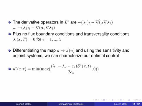
The derivative operators in L∗ are −(λ1)t −∇(α∇λ1)... −(λ5)t −∇(αv∇λ5)
Plus no flux boundary conditions and transversality conditionsλi(x, T ) = 0 for i = 1, ..., 5
Differentiating the map u→ J(u) and using the sensitivity andadjoint systems, we can characterize our optimal control
u∗(x, t) = min(max((λ1 − λ2 − c2)S∗(x, t)
2c3, 0))
Lenhart (UTK) Management Strategies June 2, 2018 11 / 52

Numerical Simulations
Forward-Backward sweep for optimality system with PDEs solvedby finite elements.Data from Rio Grande do Norte state in BrazilSome parameters from literature and other parameters wereestimatedFor estimation, used incidence from simulated system and data
Yij =
∫ tj+τ
tj
∫ωi
(βSIv + βdSI) dxdt.
Least Squares Approach with normalized residual:
R =
√√√√√√√∑i,j
(Yij − Yij
)2∑i,j
(Yij)2 .
Lenhart (UTK) Management Strategies June 2, 2018 12 / 52

Data set
2015
epi
dem
iolo
gica
l wee
k
25
20
15
10
1234567Cities
8910111213
0
1000
1500
500
Incid
en
ce
1: Santa Cruz
2: São Gonçalo do Amarante
3: Rio do Fogo
4: João Câmara
5: Apodi
6: Santo Antônio
7: Areia Branca
8: Parnamirim
9: Canguaretama
10: Caicó
11: Ceará Mirim
12: Mossoró
13: Natal
Figure: Incidence in selected cities by 2015 weeks, accounted forunder-reporting of cases.
Lenhart (UTK) Management Strategies June 2, 2018 13 / 52

Spatial region for simulations
x (km)
0 50 100 150 200 250 300 350
y (
km
)
0
50
100
150
200
Apodi
Areia Branca
CaicóCanguaretama
Ceará MirimJoão Câmara
Mossoró
Natal
Parnamirim
Rio do fogo
Santa CruzSanto Antônio
São Gonçalo do Amarante
Figure: Finite elements mesh and city locations.
Source term due to immigration added at 7 and 21 days in thehuman infected PDE
Lenhart (UTK) Management Strategies June 2, 2018 14 / 52

Parameter valuesTable: Parameters used in simulations
Values Units
β 1.28× 10⁻⁵ 1/(mosq./km2 days)βv 1.55× 10⁻² 1/(hum./km2 days)βd 0 1/(hum./km2 days)1/δ 15 days1/rv 14 days1/µv 14 daysκv 321.4 mosq./km2
α 5 km2/daysαI 5 km2/daysαv 0.315 km2/daysc1 66.67 ($/hum.)/daysc2 100 $/hum.c3 1000 $/(km2/days)
umin 0 1/daysumax 0.005 1/days
Lenhart (UTK) Management Strategies June 2, 2018 15 / 52

Initial conditions for simulations
Initial conditions :
S : 3.4 million distributed over space.
I : small amount in one city.
R : none.
Sv : 17 million distributed over space.
Iv : none.
Two sources of infecteds added in locations indicated by the data
Lenhart (UTK) Management Strategies June 2, 2018 16 / 52

No control
x (km)
0 100 200 300
y (
km
)
0
100
200
I(x,y,35)
0
0.2
0.4
x (km)
0 100 200 300
y (
km
)
0
100
200
I(x,y,52)
0
0.5
1
x (km)
0 100 200 300
y (
km
)
0
100
200
I(x,y,70)
0
1
2
x (km)
0 100 200 300
y (
km
)
0
100
200
I(x,y,91)
0
2
4
x (km)
0 100 200 300
y (
km
)
0
100
200
I(x,y,112)
0
2
4
x (km)
0 100 200 300
y (
km
)
0
100
200
I(x,y,140)
0
2
4
Figure: Solutions at different times, no control. The three infection sourcesspread over space. Difference in scales.
Lenhart (UTK) Management Strategies June 2, 2018 17 / 52

Control starting at t = 35 days
x (km)
0 100 200 300
y (
km
)
0
100
200
I(x,y,35)
0
0.2
0.4
x (km)
0 100 200 300
y (
km
)
0
100
200
I(x,y,52)
0
0.5
1
x (km)
0 100 200 300
y (
km
)
0
100
200
I(x,y,70)
0
1
2
x (km)
0 100 200 300
y (
km
)
0
100
200
I(x,y,91)
0
1
2
3
x (km)
0 100 200 300
y (
km
)
0
100
200
I(x,y,112)
0
1
2
3
x (km)
0 100 200 300
y (
km
)
0
100
200
I(x,y,140)
0
1
2
x (km)
0 100 200 300
y (
km
)
0
100
200
u(x,y,35) ×10-3
0
2
4
x (km)
0 100 200 300
y (
km
)
0
100
200
u(x,y,70) ×10-3
0
2
4
x (km)
0 100 200 300
y (
km
)
0
100
200
u(x,y,112) ×10-5
0
2
4
Figure: Solutions at different times, control starting at t = 35 days. Differencein scales.
Lenhart (UTK) Management Strategies June 2, 2018 18 / 52

Control starting at t = 52 days
x (km)
0 100 200 300
y (
km
)
0
100
200
I(x,y,35)
0
0.2
0.4
x (km)
0 100 200 300
y (
km
)
0
100
200
I(x,y,52)
0
0.5
1
x (km)
0 100 200 300
y (
km
)
0
100
200
I(x,y,70)
0
1
2
x (km)
0 100 200 300
y (
km
)
0
100
200
I(x,y,91)
0
1
2
3
x (km)
0 100 200 300
y (
km
)
0
100
200
I(x,y,112)
0
1
2
3
x (km)
0 100 200 300
y (
km
)
0
100
200
I(x,y,140)
0
1
2
3
x (km)
0 100 200 300
y (
km
)
0
100
200
u(x,y,52) ×10-3
0
2
4
x (km)
0 100 200 300
y (
km
)
0
100
200
u(x,y,70) ×10-3
0
2
4
x (km)
0 100 200 300
y (
km
)
0
100
200
u(x,y,112) ×10-5
0
2
4
Figure: Solutions at different times, control starting at t = 52 days. Differencein scales.
Lenhart (UTK) Management Strategies June 2, 2018 19 / 52
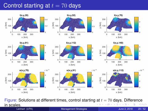
Control starting at t = 70 days
x (km)
0 100 200 300
y (
km
)
0
100
200
I(x,y,35)
0
0.2
0.4
x (km)
0 100 200 300
y (
km
)
0
100
200
I(x,y,52)
0
0.5
1
x (km)
0 100 200 300
y (
km
)
0
100
200
I(x,y,70)
0
1
2
x (km)
0 100 200 300
y (
km
)
0
100
200
I(x,y,91)
0
2
4
x (km)
0 100 200 300
y (
km
)
0
100
200
I(x,y,112)
0
1
2
3
x (km)
0 100 200 300
y (
km
)
0
100
200
I(x,y,140)
0
1
2
3
x (km)
0 100 200 300
y (
km
)
0
100
200
u(x,y,70) ×10-3
0
2
4
x (km)
0 100 200 300
y (
km
)
0
100
200
u(x,y,91) ×10-3
0
2
4
x (km)
0 100 200 300
y (
km
)
0
100
200
u(x,y,112) ×10-3
0
2
4
Figure: Solutions at different times, control starting at t = 70 days. Differencein scales.
Lenhart (UTK) Management Strategies June 2, 2018 20 / 52
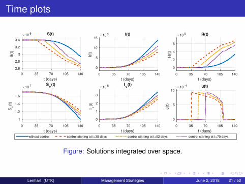
Time plots
t (days)
0 35 70 105 140
S(t
)
×10 6
2.6
2.8
3
3.2
3.4
S(t)
t (days)
0 35 70 105 140
I(t)
×10 4
0
5
10
15I(t)
t (days)
0 35 70 105 140
R(t
)
×10 5
0
2
4
6
R(t)
t (days)
0 35 70 105 140
Sv(t
)
×10 7
1
1.2
1.4
1.6
Sv(t)
t (days)
0 35 70 105 140
I v(t
)×10 6
0
1
2
3
Iv(t)
without control control starting at t=35 days control starting at t=52 days control starting at t=70 days
t (days)
0 35 70 105 140
u(t
)
×10 -4
0
5
10u(t)
Figure: Solutions integrated over space.
Lenhart (UTK) Management Strategies June 2, 2018 21 / 52
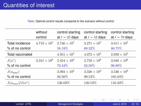
Quantities of interest
Table: Optimal control results compared to the scenario without control
without control starting control starting control startingcontrol at t = 35 days at t = 52 days at t = 70 days
Total incidence 4.719× 10⁵ 2.746× 10⁵ 3.271× 10⁵ 3.811× 10⁵
% of no control 58.18% 69.32% 80.75%
Total vaccinated 4.951× 10⁵ 4.072× 10⁵ 2.939× 10⁵
J(u∗) 3.341× 10⁸ 2.454× 10⁸ 2.759× 10⁸ 3.040× 10⁸
% of no control 73.44% 82.58% 90.98%
J(umax) 3.093× 10⁸ 3.326× 10⁸ 3.536× 10⁸
% of no control 92.56% 99.53% 105.83%
J(umax)/J(u∗) 126.03% 120.53% 116.33%
Lenhart (UTK) Management Strategies June 2, 2018 22 / 52

Conclusions
Successful application of vaccination using optimal control.
Model has been applied to real data from Brazil.
Global sensitivity analysis performed with optimal control J(u∗)value as output.
Other kinds of control could be applied and we are currentlyworking on that.
Same model can be adapted to other similar diseases.
In future work, we are including better spatial varying ICs andefficacy of vaccine.
Lenhart (UTK) Management Strategies June 2, 2018 23 / 52
Second Part
Assessing the Economic Tradeoffs Between Prevention andSuppression of Forest Fires
collaboratorsBetsy HeinesCharles Sims
GOALCombine optimal control, ecology, and economics in order todetermine the optimal fire prevention and suppression spendingby maximizing the value of a forest under threat of fire usingPontryagin’s Maximum Principle.
Lenhart (UTK) Management Strategies June 2, 2018 24 / 52

Introduction
The total number of forested acres burning in the US is increasing,despite fewer fires total.Federal suppression spending is increasing.
Data from www.nifc.gov
Lenhart (UTK) Management Strategies June 2, 2018 25 / 52
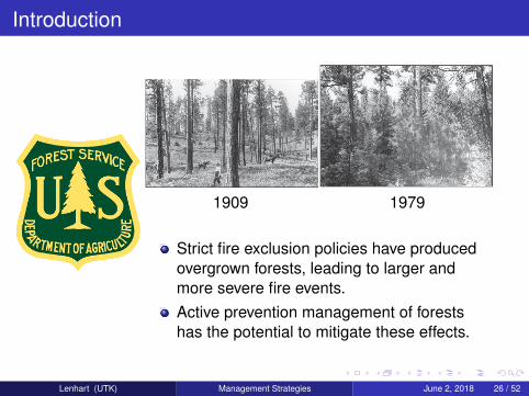
Introduction
1909 1979
Strict fire exclusion policies have producedovergrown forests, leading to larger andmore severe fire events.Active prevention management of forestshas the potential to mitigate these effects.
Lenhart (UTK) Management Strategies June 2, 2018 26 / 52

Introduction
Fire PreventionActions before a fire.Prescribed burning,mechanical thinning,...Decreases severity andprobability of ignition.
Fire SuppressionActions to control fire.Aerial spraying, boots onthe ground,...
Lenhart (UTK) Management Strategies June 2, 2018 27 / 52

Motivation
Reed, William J., and Hector Echavarria Heras. ”The conservationand exploitation of vulnerable resources.” Bulletin of MathematicalBiology 54.2-3 (1992): 185-207.
Resource management models include risk of catastrophiccollapse at an unknown time.Reed’s Method allows us to convert a stochastic problem into adeterministic optimal control problem.
Lenhart (UTK) Management Strategies June 2, 2018 28 / 52

Formulating the OC Problem
Some Assumptions:At most one fire occurs in [0, T ]. We determine the optimalprevention schedule up to the time of fire.The fire event and all associated costs are taken to beinstantaneous.The spread of fire is not modeled. However, the uncertainty in thetiming of a fire is captured through our application of Reed’sMethod.
Lenhart (UTK) Management Strategies June 2, 2018 29 / 52

Formulating the OC ProblemValue of Forest Before Fire
Let A(t) represent the number of unburned acres in an A acre forest.Suppose a fire occurs at time τ ∈ [0, T ].
Net Value of Forest Before Fire∫ τ
0
[B(A(t)
)− h(t)
]e−rtdt (2)
Flow of benefits BPrevention management spending rate h
where A(t) is given by the solution to
A′(t) = δ(A−A(t)
)with A(0) = A0. (3)
Lenhart (UTK) Management Strategies June 2, 2018 30 / 52
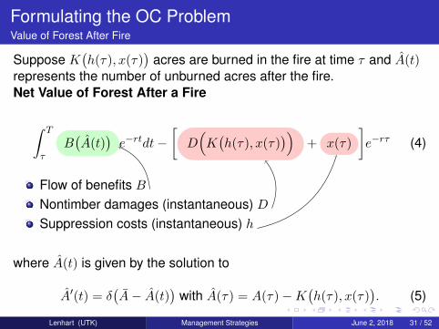
Formulating the OC ProblemValue of Forest After Fire
Suppose K(h(τ), x(τ)
)acres are burned in the fire at time τ and A(t)
represents the number of unburned acres after the fire.Net Value of Forest After a Fire
∫ T
τB(A(t)
)e−rtdt−
[D(K(h(τ), x(τ)
))+ x(τ)
]e−rτ (4)
Flow of benefits BNontimber damages (instantaneous) DSuppression costs (instantaneous) h
where A(t) is given by the solution to
A′(t) = δ(A− A(t)
)with A(τ) = A(τ)−K
(h(τ), x(τ)
). (5)
Lenhart (UTK) Management Strategies June 2, 2018 31 / 52

Formulating the OC ProblemMaximize Value of Forest After Fire
Define the optimal value of the forest after a fire by
JW ∗(τ,A(τ), h(τ)
)=
maxx(τ)
∫ T
τB(A(t)
)e−r(t−τ)dt−
[D(K(h(τ), x(τ)
))+ x(τ)
]subject to x(τ) ≥ 0
where A(t) = A−(A−
(A(τ)−K
(h(τ), x(τ)
)))e−δ(t−τ). (6)
We solve the problem above using scalar optimization with respect to xfor a given τ , A(τ), and h(τ).
Note: JW ∗(τ,A(τ), h(τ)
)will be a function with an explicit closed form
due to our functional choices.Lenhart (UTK) Management Strategies June 2, 2018 32 / 52

Formulating the OC ProblemValue of a Forest Over [0, T ] - Fire at τ ∈ [0, T ]
Suppose that a fire occurs at time τ ∈ [0, T ] and that suppressionspending is optimal, then the value of the forest over [0, T ] is∫ τ
0
[B(A(t)
)− h(t)
]e−rtdt + JW ∗
(τ,A(τ), h(τ)
)e−rτ (7)
Net value before fireNet value after fire w/ optimal suppression expenditures x∗
where
A(t) = A− (A−A0)e−δt. (8)
Lenhart (UTK) Management Strategies June 2, 2018 33 / 52

Formulating the OC ProblemValue of a Forest Over [0, T ] - No Fire
Suppose a fire does not occur in [0, T ]. Then the value of the forestover [0, T ] is
∫ T
0
[B(A(t)
)− h(t)
]e−rtdt. (9)
Benefits minus prevention over full time horizon
where
A(t) = A− (A−A0)e−δt. (10)
Lenhart (UTK) Management Strategies June 2, 2018 34 / 52

Formulating the OC ProblemTime of Fire as a Random Variable
To capture the uncertainty of the time of fire τ ∈ [0,∞), we treat it as arandom variable T .
Hazard Function:
ψ(h(t)
)= lim
∆t→0
Pr(fire in [t, t+ ∆t)| no fire up to t
)/∆t
(11)
Survivor Function:S(t) = e−
∫ t0 ψ(h(z))dz (12)
Cumulative Distribution Function:
F (t) = 1− S(t) (13)
Lenhart (UTK) Management Strategies June 2, 2018 35 / 52
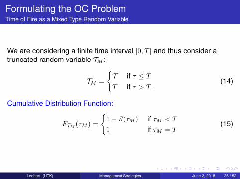
Formulating the OC ProblemTime of Fire as a Mixed Type Random Variable
We are considering a finite time interval [0, T ] and thus consider atruncated random variable TM :
TM =
T if τ ≤ TT if τ > T.
(14)
Cumulative Distribution Function:
FTM (τM ) =
1− S(τM ) if τM < T
1 if τM = T(15)
Lenhart (UTK) Management Strategies June 2, 2018 36 / 52

Formulating the OC ProblemFrom Stochastic to Deterministic
The expected value of the forest J(h) is given by the expectation, withrespect to the RV TM , of the piecewise function for the value of theforest:
J(h) = ETM
∫ τM
0
[B(A(t)
)− h(t)
]e−rtdt
+e−rτMJW ∗(τM , A(τM ), h(τM )
)if τM < T∫ T
0
[B(A(t)
)− h(t)
]e−rtdt if τM = T.
(16)
Lenhart (UTK) Management Strategies June 2, 2018 37 / 52
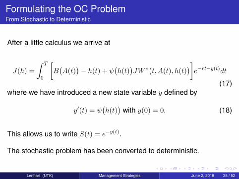
Formulating the OC ProblemFrom Stochastic to Deterministic
After a little calculus we arrive at
J(h) =
∫ T
0
[B(A(t)
)− h(t) + ψ
(h(t)
)JW ∗
(t, A(t), h(t)
)]e−rt−y(t)dt
(17)where we have introduced a new state variable y defined by
y′(t) = ψ(h(t)
)with y(0) = 0. (18)
This allows us to write S(t) = e−y(t).
The stochastic problem has been converted to deterministic.
Lenhart (UTK) Management Strategies June 2, 2018 38 / 52

The Optimal Control Problem:
maxh
∫ T
0
[B(A(t)
)− h(t) + ψ
(h(t)
)JW ∗
(t, A(t), h(t)
)]e−rt−y(t)dt (19)
subject to y′(t) = ψ(h(t)
)with y(0) = 0 (20)
h(t) ≥ 0 (21)
where A(t) = A− (A−A0)e−δt. (22)
Next, we present the conditional current-value Hamiltonian andoptimality system and introduce our chosen functional forms.
Lenhart (UTK) Management Strategies June 2, 2018 39 / 52

Conditional Current-Value Hamiltonian & OptimalitySystem
Let H be the Hamiltonian with adjoint λ. Then the conditional current-valueHamiltonian is H = ert+y(t)H with corresponding adjoint equation ρ(t) = ert+y(t)λ(t).
Conditional Current-Value Hamiltonian
H = B(A(t)
)− h(t) + ψ
(h(t)
)JW ∗(t, A(t), h(t)
)+ ρ(t)ψ
(h(t)
)(23)
Optimality Condition, in interior of control set
∂H∂h
= −1+JW ∗(t, A(t), h(t))∂ψ∂h
+∂JW ∗
∂hψ(h(t)
)+ρ(t)
∂ψ
∂h= 0 (24)
Adjoint Equation
ρ(t) = rρ(t) +B(A(t)
)− h(t) + ψ
(h(t)
)(ρ(t) + JW ∗(t, A(t), h(t)
))(25)
Transversality Conditionρ(T ) = 0 (26)
Lenhart (UTK) Management Strategies June 2, 2018 40 / 52

Functional Forms
Benefits Function : B1 - benefits parameter
B(A(t)
)= B1A(t)
Hazard Function : b - background hazard of firev - hazard management effectiveness parameter
ψ(h(t)
)= be−vh(t)
Kill Function : k - fire severity parameterk1 - severity management effectiveness parameterk2 - severity suppression effectiveness parameter
K(h, x) =k
(k1 + h)(k2 + x)
Nontimber Damage Function : c - cost parameter
D(K(h, x)
)= cK(h, x)
Lenhart (UTK) Management Strategies June 2, 2018 41 / 52

Numerical Methods
Due to the complexity of ψ and JW ∗ an explicit closed formcannot be determined for h∗ from the optimality condition.
We numerically determine h∗ by maximizing the conditionalcurrent-value Hamiltonian with respect to h at each time step.
The MATLAB function fminbnd is used to optimize h. Since thecontrol h is not bounded above, a large upper bound was used onfminbnd.
Lenhart (UTK) Management Strategies June 2, 2018 42 / 52
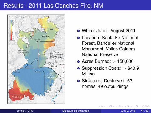
Results - 2011 Las Conchas Fire, NM
When: June - August 2011Location: Santa Fe NationalForest, Bandelier NationalMonument, Valles CalderaNational PreserveAcres Burned: > 150,000Suppression Costs: ≈ $40.9MillionStructures Destroyed: 63homes, 49 outbuildings
Lenhart (UTK) Management Strategies June 2, 2018 43 / 52

Results - Las ConchasParameter Choices
Param. Units Value JustificationA acres(thou.) 1700 size of SFNF, BNM, VCNPr /time 0.04 standard discount ratek acres(thou.)×$2 7000 k ≈ size of fire× suppression $k1 $ (mil.) 1 assumedk2 $ (mil.) 1 assumedδ /time 0.05 Pipo: 70-250 years to matureb ——– 0.2 high frequency of fires in regionc $ (mil.)/ 0.1 114 buildings destroyed,
acres(thou.) 156,000 acres burnedB1 $ (mil.) 0.02 calculated from x∗ formulav ——— 1 assumed
Lenhart (UTK) Management Strategies June 2, 2018 44 / 52
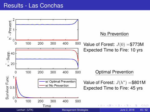
Results - Las Conchas
No Prevention
Value of Forest: J(0) =$773MExpected Time to Fire: 10 yrs
Optimal Prevention
Value of Forest: J(h∗) =$801MExpected Time to Fire: 45 yrs
Lenhart (UTK) Management Strategies June 2, 2018 45 / 52

Results - Las Conchas
Preliminary Results
When the optimal prevention management spending rate is applied,we see:
An increase in the expected value of the forest.An increase in the mean time of fire.
Lenhart (UTK) Management Strategies June 2, 2018 46 / 52

Fire Sequences
Using a different initial condition for A(t), it is possible to considersequences of fires by successively applying our optimal controlproblem.
We can determine the time of fire by sampling from the cumulativedistribution function for the time of fire random variable.
Lenhart (UTK) Management Strategies June 2, 2018 47 / 52
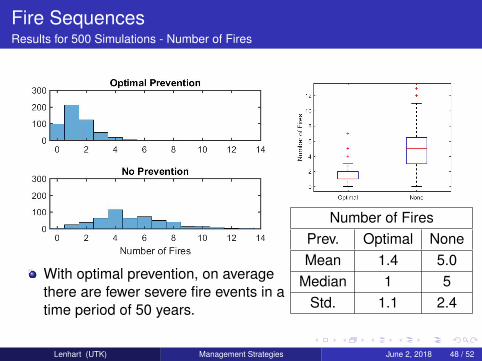
Fire SequencesResults for 500 Simulations - Number of Fires
With optimal prevention, on averagethere are fewer severe fire events in atime period of 50 years.
Number of FiresPrev. Optimal NoneMean 1.4 5.0
Median 1 5Std. 1.1 2.4
Lenhart (UTK) Management Strategies June 2, 2018 48 / 52

Fire SequencesResults for 500 Simulations - Value of the Forest
Larger mean/median for optimalprevention case.Furthermore, std. for no preventioncase is over triple the std. of optimalprevention case.
Value of Forest $MPrev. Optimal NoneMean 671 536
Median 677 556Std. 34.0 111.7
Lenhart (UTK) Management Strategies June 2, 2018 49 / 52

Fire SequencesResults for 500 Simulations - Prev. vs. Supp.
Without prevention management, on average $236M spent onsuppression in 50 years.With prevention management, on average $42.4M spent onsuppression and $65M spent on prevention management in 50years.
Adopting prevention management could lead to an 82% reduction insuppression spending and a 55% reduction in spending overall.
Lenhart (UTK) Management Strategies June 2, 2018 50 / 52

Conclusions
From our work with fire sequences, we see that on average withprevention management:
The overall value of a forest is increased by 25% and has lessvariation than when no prevention management efforts are made.
There is a 72% reduction in the number of forest fires.Furthermore, the forest is at less risk for fire.
There is an 82% reduction in suppression spending and a 55%reduction in management and suppression spending in total.
This work showcases a valuable tool which could guide forestmanagers and policymakers in their development of forest firemanagement plans.
Lenhart (UTK) Management Strategies June 2, 2018 51 / 52

Acknowledgments and Thanks!
National Institute for Mathematical and Biological Synthesiswww.nimbios.org
THANK YOU
Lenhart (UTK) Management Strategies June 2, 2018 52 / 52