optimal control of wind farms with energy storage under ... · pdf fileoptimal control of wind...
TRANSCRIPT
eeh power systemslaboratory
Andreas Horst Venzke
Optimal Control of Wind Farms withEnergy Storage under Grid Code
Compliance
Semester ThesisPSL1503
EEH – Power Systems LaboratorySwiss Federal Institute of Technology (ETH) Zurich
Examiner: Prof. Dr. Goran AnderssonSupervisor: M.Sc. Philipp Fortenbacher
Zurich, June 4, 2015


Abstract
The further integration of wind energy into electrical power systems posesoperational challenges as the variability in wind power reduces transient sta-bility. To guarantee a stable and secure power system operation, maximumallowable power ramps are defined in grid codes that transmission serviceoperators (TSOs) specify. In this thesis it shall be investigated how a windpower system with energy storage can be optimally controlled to complywith power gradient restrictions. For this purpose, the kinetic energy in themotion of the wind turbine rotor is utilized and an external battery storageis employed.
The main contributions of this thesis are the design, implementation andvalidation of a supervisory control scheme. The control consists of a modelpredictive controller and a proportional integral controller for wind turbinepitch control. The model predictive controller serves as supervisory controland provides set-points for the wind turbine control and for the battery.An existing optimal control formulation using a single order wind turbinemodel is further extended including a battery model capturing fast transientdynamics and a battery degradation objective. In order to assess the per-formance of the proposed supervisory control system, a higher order windturbine model is used. Energy yield, power gradients and loading on thewind turbine are evaluated for different wind scenarios. It is found thatthe proposed supervisory control system substantially mitigates power gra-dients. If a maximum rotor speed of 1.5 times the rated speed is allowed anda battery with 20% of the rated wind turbine power is used, the energy yieldamounts to 97.0% compared to a standard proportional integral controller.For this configuration, the maximum power gradient is reduced by 78.5%and the standard deviation by 88.7%. The damage equivalent load of thetower root bending moment increases by 20%. For the torsion moment ofthe rotor shaft a slight decrease by 4.5% is observed. Hence, the proposedcontrol is able to comply with tight power ramp restrictions while keepingenergy losses and increase in turbine loading to a minimum.
i

Contents
List of Acronyms iv
List of Symbols v
List of Figures viii
List of Tables x
1 Introduction 11.1 Scope of Thesis . . . . . . . . . . . . . . . . . . . . . . . . . . 11.2 Grid Code Requirements for Wind Farms . . . . . . . . . . . 31.3 Structure . . . . . . . . . . . . . . . . . . . . . . . . . . . . . 3
2 System Component Modeling 52.1 Fundamentals of Wind Turbine Control . . . . . . . . . . . . 62.2 Wind Turbine Model . . . . . . . . . . . . . . . . . . . . . . . 8
2.2.1 Single Degree of Freedom Model . . . . . . . . . . . . 82.2.2 Higher Order Model . . . . . . . . . . . . . . . . . . . 9
2.3 Rotor Inertia as Kinetic Energy Storage . . . . . . . . . . . . 102.4 Linearized Battery Model . . . . . . . . . . . . . . . . . . . . 12
3 Optimal Control of Wind Turbine with Energy Storage 133.1 Optimal Control Formulation . . . . . . . . . . . . . . . . . . 13
3.1.1 Dynamics, Constraints and Available Power Function 133.1.2 Existing Set of Objectives . . . . . . . . . . . . . . . . 163.1.3 Extended Set of Objectives . . . . . . . . . . . . . . . 173.1.4 Optimization Problem for Wind Turbine . . . . . . . . 183.1.5 Optimization Problem for Wind Farm . . . . . . . . . 19
3.2 Controller Design . . . . . . . . . . . . . . . . . . . . . . . . . 213.2.1 Model Predictive Control . . . . . . . . . . . . . . . . 223.2.2 Proportional Integral Control . . . . . . . . . . . . . . 223.2.3 Supervisory Control System . . . . . . . . . . . . . . . 23
ii

CONTENTS iii
4 Implementation and Results 254.1 Simulation Setup . . . . . . . . . . . . . . . . . . . . . . . . . 25
4.1.1 Model Predictive Control . . . . . . . . . . . . . . . . 254.1.2 Supervisory Control System . . . . . . . . . . . . . . . 27
4.2 Sizing of Energy Storage using Step Response . . . . . . . . . 294.3 Performance of Designed Controllers under Different Wind
Scenarios . . . . . . . . . . . . . . . . . . . . . . . . . . . . . 33
5 Conclusion 415.1 Summary of Results . . . . . . . . . . . . . . . . . . . . . . . 415.2 Outlook . . . . . . . . . . . . . . . . . . . . . . . . . . . . . . 42
Bibliography 43

List of Acronyms
ADC Actuator Duty CycleDEL Damage Equivalent LoadKiBaM Kinetic Battery ModelLiDAR Light Detection And RangingLP Linear ProgramMPC Model Predictive ControlNREL National Renewable Energy LaboratoryNWTC National Wind Technology CenterPI Proportional IntegralSOC State of ChargeTSR Tip Speed RatioTSO Transmission System OperatorYALMIP Yet Another Linear Matrix Inequality Parser
iv

List of Symbols
Pgrid power injection into the gridPg wind turbine generator powerP ref
g wind turbine generator power reference
Pw extracted wind powerPav available power functionK kinetic energy stored in rotor
K derivative of kinetic energyTg generator torqueTg,max maximum generator torqueTshaft shaft momentFtow tower forceCT thrust coefficientTr rotor torqueβ blade pitch angleβref blade pitch angle referencePwind power contained in wind flowρ density of airA cross-sectional rotor areaN gear ratioηg generator efficiencyCP power coefficientCP,max maximum power coefficientλ tip speed ratioR rotor radiusωr rotor speedωr,max maximum rotor speedωr,min minimum rotor speedωref
r rotor speed referenceωr derivative of rotor speedωref
g generator speed reference
ωr generator speedJ total inertiaJr rotor inertia
v

CONTENTS vi
Jg generator inertiaBshaft viscous friction constantKshaft torsion spring constantξ shaft torsion angle
ξ derivative of shaft torsion angle
Tg derivative of generator torquevw wind speedvforecast
w wind speed forecastPref power referenceτg generator time constantmtow tower massx tower deflectionx tower deflection velocityx tower deflection accelerationBtow tower damping constantKtow tower spring constantτβ pitch actuator time constantτd pitch actuator time delay
β pitch rateKβ pitch actuator proportional gain
β derivative of the pitch rateβm measured pitch anglePbat battery powerP ref
bat battery power referencex1,bat first charge wellx2,bat second charge wellcw width of the first wellcr valve conductancePgen discharging powerPload charging powerηgen discharging battery efficiencyηload charging battery efficiencyCbat battery capacityJ objective function in the optimizationζ weight assigned to objective functionζE objective energy yieldJE objective weight energy yieldζG,P objective power gradientJG,P objective weight power gradientζP objective power variationJP objective weight power variationJr objective rotor over-speedζr objective weight rotor over-speed

CONTENTS vii
ζav objective available powerJav objective weight available powerζr,G objective kinetic energy gradientJr,G objective weight kinetic energy gradientζg objective generator powerJg objective weight generator powerζchg first objective battery powerJchg first objective weight battery powerζchg,max second objective battery powerJchg,max second objective weight battery powerJSOC objective battery degradationζSOC objective weight battery degradationx dynamic state vectorz algebraic state vectoru control vectorxWF dynamic state vector for wind farmzWF algebraic state vector for wind farmuWF control vector for wind farmAbat dynamic state matrix for batteryBbat dynamic control matrix for batteryA dynamic state matrix for system dynamicsB dynamic control matrix for system dynamicsGP power ramp restrictionGK kinetic energy ramp restrictionNp prediction horizonTs sampling timeKp proportional gainKi integral gain
List of Figures
1.1 System overview with controller, battery and wind power sys-tem . . . . . . . . . . . . . . . . . . . . . . . . . . . . . . . . 2
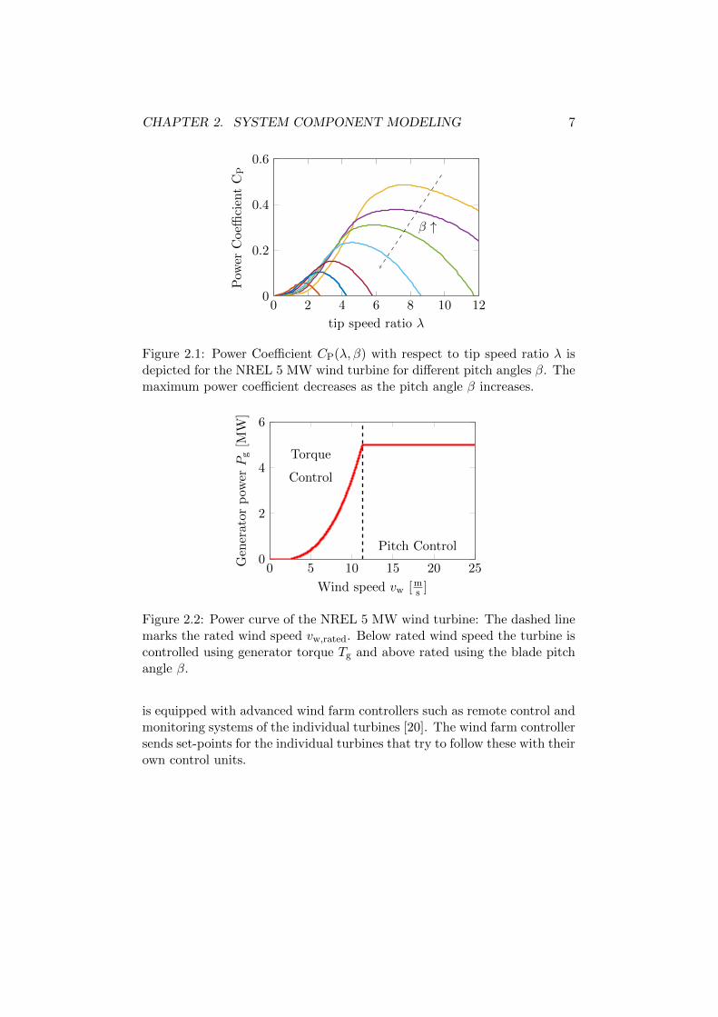
2.1 Power Coefficient CP(λ, β) with respect to tip speed ratio λis depicted for the NREL 5 MW wind turbine for differentpitch angles β. The maximum power coefficient decreases asthe pitch angle β increases. . . . . . . . . . . . . . . . . . . . 7
2.2 Power curve of the NREL 5 MW wind turbine: The dashedline marks the rated wind speed vw,rated. Below rated windspeed the turbine is controlled using generator torque Tg andabove rated using the blade pitch angle β. . . . . . . . . . . . 7
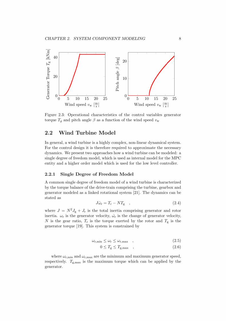
2.3 Operational characteristics of the control variables generatortorque Tg and pitch angle β as a function of the wind speed vw 8
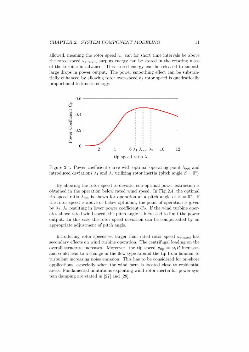
2.4 Power coefficient curve with optimal operating point λopt andintroduced deviations λ1 and λ2 utilizing rotor inertia (pitchangle β = 0◦) . . . . . . . . . . . . . . . . . . . . . . . . . . . 11
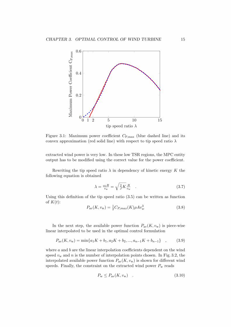
3.1 Maximum power coefficient CP,max (blue dashed line) andits convex approximation (red solid line) with respect to tipspeed ratio λ . . . . . . . . . . . . . . . . . . . . . . . . . . . 15
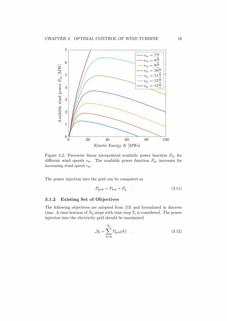
3.2 Piecewise linear interpolated available power function Pav fordifferent wind speeds vw. The available power function Pav
increases for increasing wind speed vw. . . . . . . . . . . . . . 163.3 Simplified AEOLUS SWF toolbox structure with proportional
integral controller for pitch control and look-up table for torquecontrol. The demanded generator power P ref
g can be specifiedexternally. . . . . . . . . . . . . . . . . . . . . . . . . . . . . . 23
3.4 Open and closed-loop supervisory control system . . . . . . . 24
4.1 Reference trajectory for rotational wind speed ωrefr and the
three modifications applied to the trajectory. The wind stepis from 12 m
s to 10 ms . (Np = 200) . . . . . . . . . . . . . . . . 28
4.2 Overview of the connection of high level controller (MPC)and low level controller (PI) . . . . . . . . . . . . . . . . . . . 29
viii
LIST OF FIGURES ix
4.3 Step response of the model predictive controller with a batterysize of 0.8 MW and enabled 50% rotor over-speed. The windspeed drops from 12 m
s to 10 ms . (Np = 200) . . . . . . . . . . 30
4.4 Operation below rated wind speed: The percentage of step en-ergy extracted is shown with respect to chosen battery power.The variation in power amounts to ∆P = 1.7 MW. . . . . . . 31
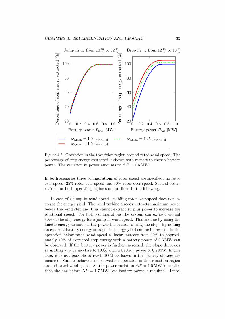
4.5 Operation in the transition region around rated wind speed:The percentage of step energy extracted is shown with respectto chosen battery power. The variation in power amounts to∆P = 1.5 MW. . . . . . . . . . . . . . . . . . . . . . . . . . . 32
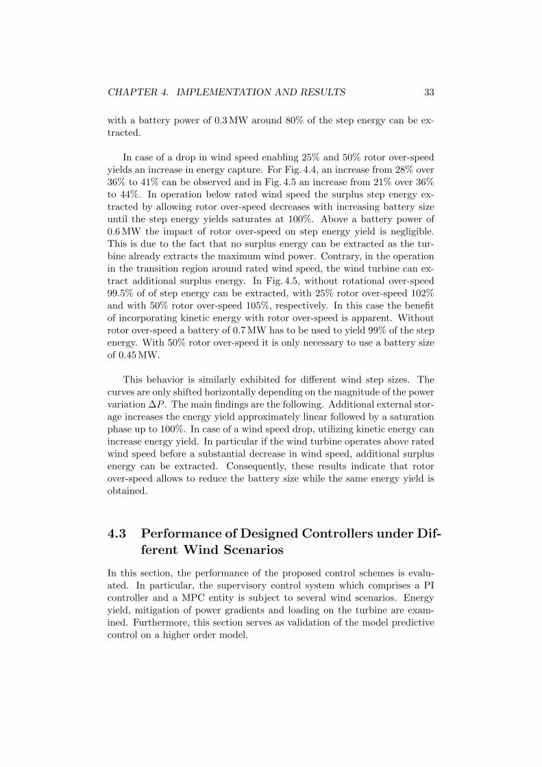
4.6 The output of the supervisory control system (rotor over-speed enabled and Pbat = 0.8MW) is compared to the bench-mark PI controller and to the reference provided by the MPCcontroller. . . . . . . . . . . . . . . . . . . . . . . . . . . . . . 35
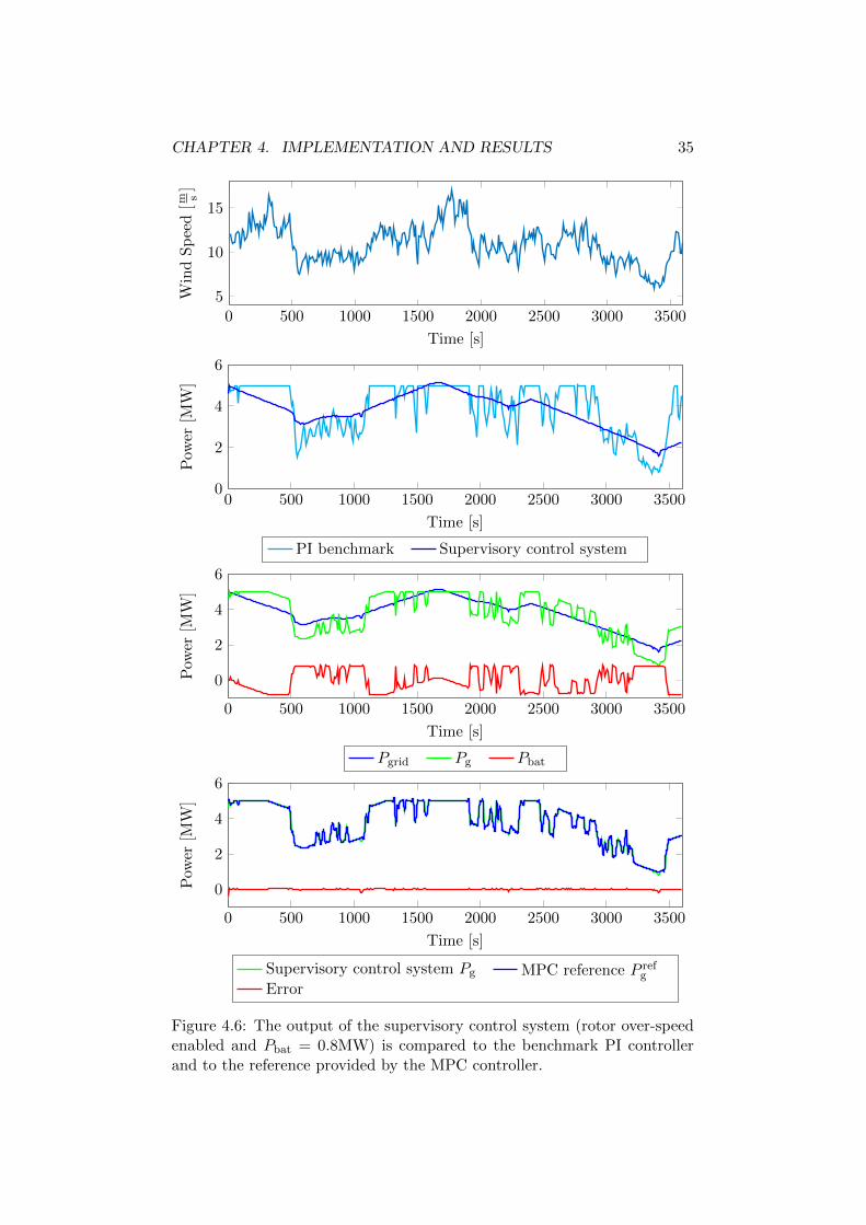
4.7 Kinetic energy compared between the supervisory control sys-tem (rotor over-speed enabled and Pbat = 0.8 MW) and theunmodified and modified kinetic energy reference provided tothe PI controller . . . . . . . . . . . . . . . . . . . . . . . . . 36
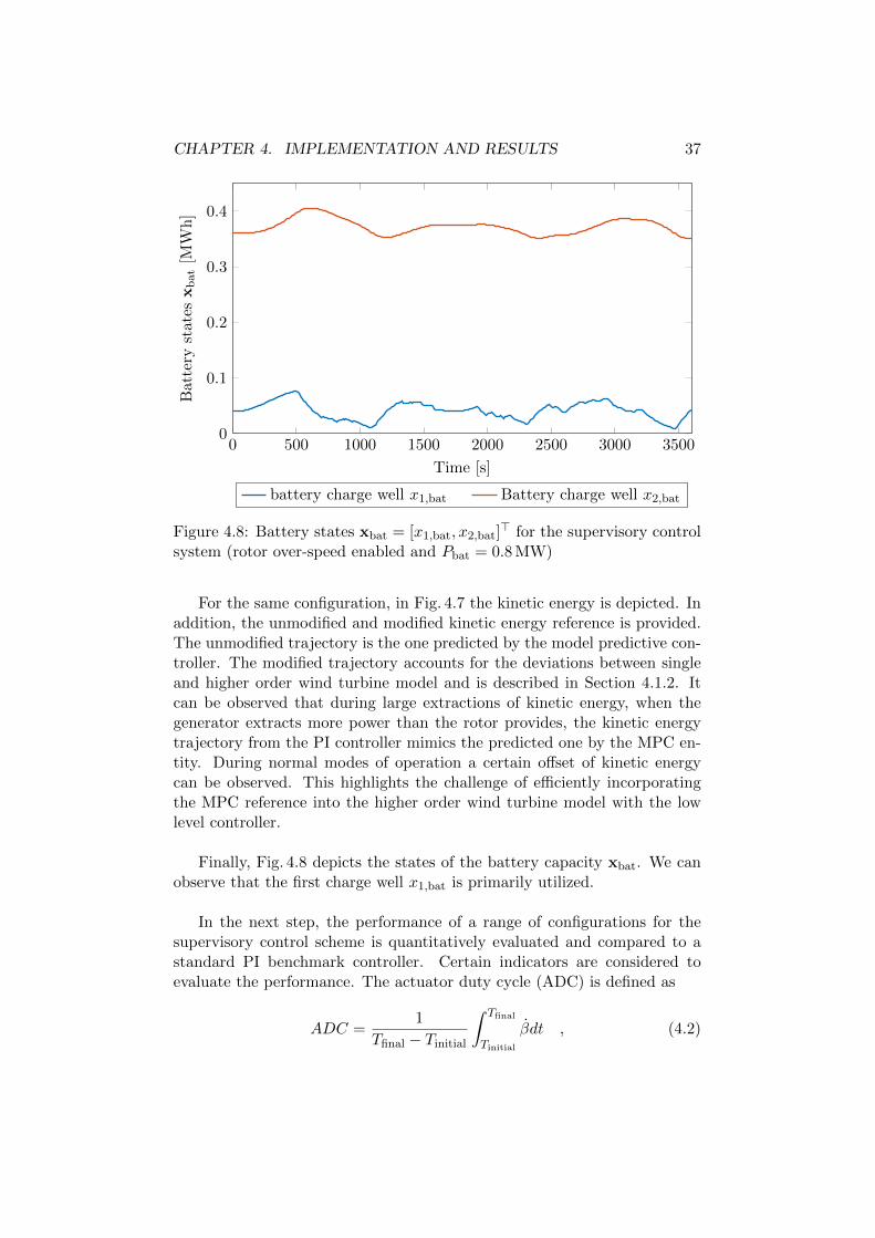
4.8 Battery states xbat = [x1,bat, x2,bat]> for the supervisory con-
trol system (rotor over-speed enabled and Pbat = 0.8 MW) . . 374.9 Comparison of power gradients between supervisory control
system with rotor over-speed enabled and a battery size ofPbat = 1.0MW and the benchmark PI for three differenthourly scenarios: The red line indicates the gradient restric-tion GP = 0.0025MW
s . . . . . . . . . . . . . . . . . . . . . . . 40

List of Tables
2.1 Specifications of the 5MW NREL wind turbine . . . . . . . . 5
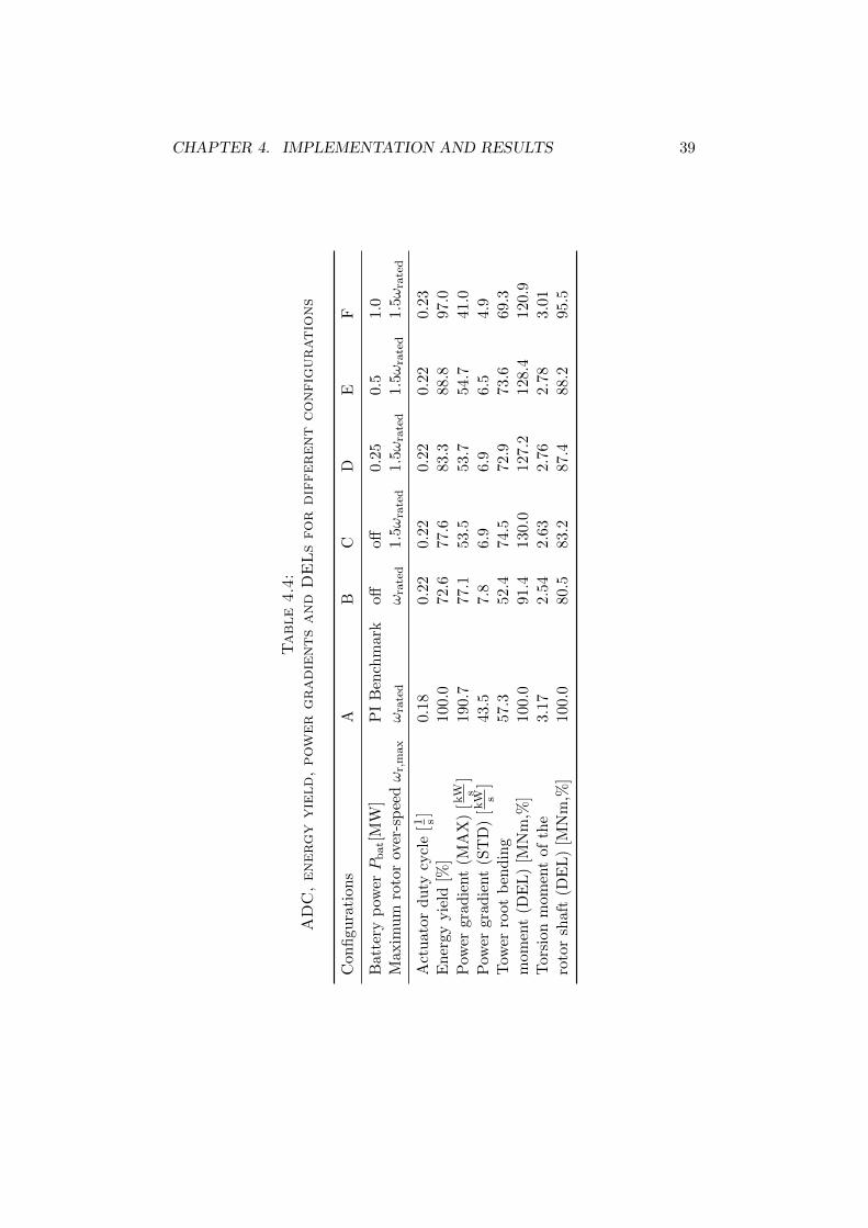
4.1 Battery model specifications . . . . . . . . . . . . . . . . . . . 254.2 Optimal control weights specifications . . . . . . . . . . . . . 264.3 Additional specifications . . . . . . . . . . . . . . . . . . . . . 264.4 ADC, energy yield, power gradients and DELs for different
configurations . . . . . . . . . . . . . . . . . . . . . . . . . . . 39
x
Chapter 1
Introduction
1.1 Scope of Thesis
Wind energy is continuously growing and plays a significant role in the tran-sition process to sustainable power production. In several countries aroundthe world e.g. United Kingdom, Germany, Denmark and also in the UnitedStates of America the share of wind power in the electricity mix is constantlyincreasing [1]. Among these countries Denmark has set the most ambitiousgoal with 50% of electricity generated from wind power by 2020 [2]. Thefurther integration of wind energy into electrical power systems poses opera-tional challenges as the variability in wind power reduces transient stability.This will require wind turbines, especially wind farms, to produce electricitywith a high power quality and further decrease the necessity for external sta-bilizing measures. To guarantee a stable and secure power system operation,maximum allowable power ramps are defined in grid codes that transmissionservice operators (TSOs) specify.
In this thesis it shall be investigated how a wind power system with useof its kinetic rotational energy and the use of an external battery energystorage can be optimally controlled to comply with tight power gradient re-strictions. The main focus is to decrease the effect of wind speed variationson the power injection into the grid. In order to deploy a control systembeing effectively capable of mitigating power gradients, a wind forecast hasto be incorporated. Therefore, an optimal control problem is formulatedwhich is implemented using model predictive control (MPC). MPC for windturbines is a well established topic in research [3]. A review on applicationsof MPC for wind turbines is given in [4].
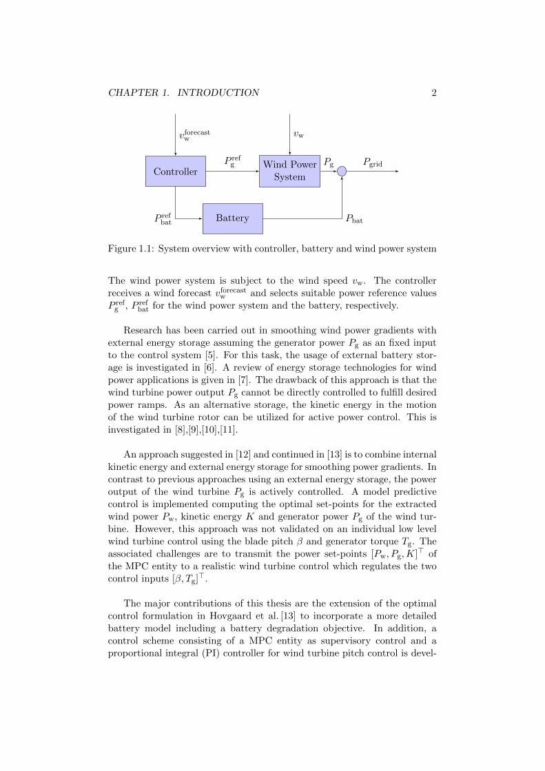
In Fig. 1.1, the basic system comprising a wind power system and bat-tery energy storage is depicted. The power injection into the grid Pgrid iscomposed of the wind turbine generator power Pg and battery power Pbat.
1
CHAPTER 1. INTRODUCTION 2
ControllerWind Power
System
P refg
Battery
vw
Pg
vforecastw
P refbat Pbat
Pgrid
Figure 1.1: System overview with controller, battery and wind power system
The wind power system is subject to the wind speed vw. The controllerreceives a wind forecast vforecast
w and selects suitable power reference valuesP ref
g , P refbat for the wind power system and the battery, respectively.
Research has been carried out in smoothing wind power gradients withexternal energy storage assuming the generator power Pg as an fixed inputto the control system [5]. For this task, the usage of external battery stor-age is investigated in [6]. A review of energy storage technologies for windpower applications is given in [7]. The drawback of this approach is that thewind turbine power output Pg cannot be directly controlled to fulfill desiredpower ramps. As an alternative storage, the kinetic energy in the motionof the wind turbine rotor can be utilized for active power control. This isinvestigated in [8],[9],[10],[11].
An approach suggested in [12] and continued in [13] is to combine internalkinetic energy and external energy storage for smoothing power gradients. Incontrast to previous approaches using an external energy storage, the poweroutput of the wind turbine Pg is actively controlled. A model predictivecontrol is implemented computing the optimal set-points for the extractedwind power Pw, kinetic energy K and generator power Pg of the wind tur-bine. However, this approach was not validated on an individual low levelwind turbine control using the blade pitch β and generator torque Tg. Theassociated challenges are to transmit the power set-points [Pw, Pg,K]> ofthe MPC entity to a realistic wind turbine control which regulates the twocontrol inputs [β, Tg]>.
The major contributions of this thesis are the extension of the optimalcontrol formulation in Hovgaard et al. [13] to incorporate a more detailedbattery model including a battery degradation objective. In addition, acontrol scheme consisting of a MPC entity as supervisory control and aproportional integral (PI) controller for wind turbine pitch control is devel-
CHAPTER 1. INTRODUCTION 3
oped and implemented. The performance is evaluated under different windscenarios.
1.2 Grid Code Requirements for Wind Farms
In this section, a short review on grid code requirements for wind farms ispresented. A more comprehensive and detailed report is given in [14]. Themain requirements stated in grid codes are dealing with active and reactivepower control, voltage and frequency operating limits and wind farm be-havior during grid disturbances [15]. During disturbances recent grid codesrequire wind farms to remain connected and support the grid during andafter a fault [14].
The focus in this thesis is on active power control. This term refers tothe ability of a wind power system to regulate its active power output to adefined level at a defined ramp rate. Thereby frequency stability is ensured,overloading of transmission lines is prevented and the effect of wind powerdynamics on the grid is minimized [14]. Concerning active power control,the following three specifications are made [16]:
• The absolute power constraint demands that the power output of awind farm remains below a specified threshold.
• The delta production constraint requires that a wind farm maintainsan active power reserve.
• The power gradient constraint limits the rate of change of power out-put. Under normal conditions many grid codes require a ramp-downrate of less than 10% of the rated power per minute.
Curtailment of wind power plants is necessary to fulfill the requirementson active power control and can incur significant energy losses. Grid codesare observed to be tightened as the share of wind power in the electricity mixincreases. Therefore it is worthwhile to investigate control techniques whichare able to meet the requirements without significant loss in energy yield.Furthermore, negative power ramp restrictions are still largely exempted tobe followed but pose challenges concerning transient system stability. Froma system point-of-view, it is desirable that wind power plants are also able tomitigate the effect of large wind speed drops on their power output. In thisthesis we suggest a control capable of fulfilling the power ramp constraints.
1.3 Structure
Chapter 2 focuses on the modeling of the system components. A single orderand a higher order wind turbine model are introduced. The concept of using

CHAPTER 1. INTRODUCTION 4
the kinetic energy stored in the motion of the wind turbine rotor to smoothpower gradients is presented. Furthermore, a linearized battery model cap-turing fast transient dynamics is described. In chapter 3, the optimal controlproblem is formulated, refined and further extended by incorporating a de-tailed battery model and a degradation objective. The design of the MPCentity, the PI controller and the combined supervisory control scheme isoutlined. In chapter 4, the implementation of the MPC entity and the su-pervisory control system is explained. The sizing of the energy storage withrespect to energy yield is estimated using step responses. The performanceof the supervisory control system is assessed. Energy yield, power gradientsand loading are analyzed for different wind scenarios. Finally, a conclusionis drawn and an outlook into further extensions is given.
Chapter 2
System ComponentModeling
The system considered for control design consists of one or several wind tur-bines which are able to utilize their rotational kinetic energy coupled with abattery storage system. After an introduction to the fundamentals of windturbine control, descriptions of the system components are presented. Inparticular, a single and a higher order wind turbine model are introduced.Furthermore, the use of rotor inertia as kinetic energy storage is explained.Finally, a linearized battery model is presented capturing fast transient dy-namics.
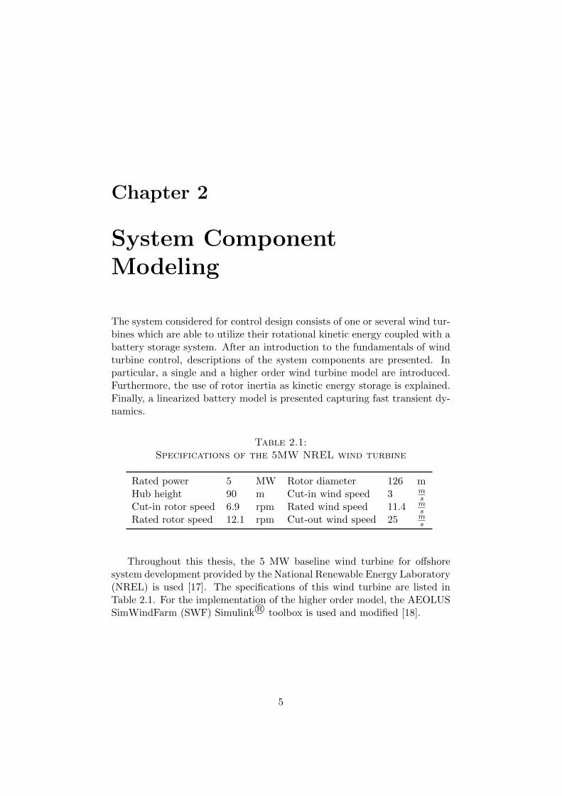
Table 2.1:Specifications of the 5MW NREL wind turbine
Rated power 5 MW Rotor diameter 126 mHub height 90 m Cut-in wind speed 3 m
sCut-in rotor speed 6.9 rpm Rated wind speed 11.4 m
sRated rotor speed 12.1 rpm Cut-out wind speed 25 m
s
Throughout this thesis, the 5 MW baseline wind turbine for offshoresystem development provided by the National Renewable Energy Laboratory(NREL) is used [17]. The specifications of this wind turbine are listed inTable 2.1. For the implementation of the higher order model, the AEOLUSSimWindFarm (SWF) Simulink R© toolbox is used and modified [18].
5
CHAPTER 2. SYSTEM COMPONENT MODELING 6
2.1 Fundamentals of Wind Turbine Control
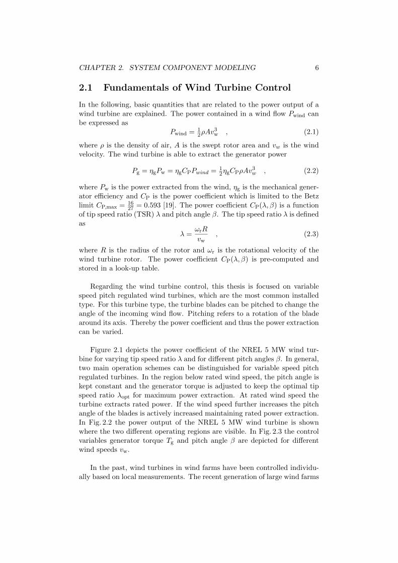
In the following, basic quantities that are related to the power output of awind turbine are explained. The power contained in a wind flow Pwind canbe expressed as
Pwind = 12ρAv
3w , (2.1)
where ρ is the density of air, A is the swept rotor area and vw is the windvelocity. The wind turbine is able to extract the generator power
Pg = ηgPw = ηgCPPwind = 12ηgCPρAv
3w , (2.2)
where Pw is the power extracted from the wind, ηg is the mechanical gener-ator efficiency and CP is the power coefficient which is limited to the Betzlimit CP,max = 16
27 = 0.593 [19]. The power coefficient CP(λ, β) is a functionof tip speed ratio (TSR) λ and pitch angle β. The tip speed ratio λ is definedas
λ =ωrR
vw, (2.3)
where R is the radius of the rotor and ωr is the rotational velocity of thewind turbine rotor. The power coefficient CP(λ, β) is pre-computed andstored in a look-up table.
Regarding the wind turbine control, this thesis is focused on variablespeed pitch regulated wind turbines, which are the most common installedtype. For this turbine type, the turbine blades can be pitched to change theangle of the incoming wind flow. Pitching refers to a rotation of the bladearound its axis. Thereby the power coefficient and thus the power extractioncan be varied.
Figure 2.1 depicts the power coefficient of the NREL 5 MW wind tur-bine for varying tip speed ratio λ and for different pitch angles β. In general,two main operation schemes can be distinguished for variable speed pitchregulated turbines. In the region below rated wind speed, the pitch angle iskept constant and the generator torque is adjusted to keep the optimal tipspeed ratio λopt for maximum power extraction. At rated wind speed theturbine extracts rated power. If the wind speed further increases the pitchangle of the blades is actively increased maintaining rated power extraction.In Fig. 2.2 the power output of the NREL 5 MW wind turbine is shownwhere the two different operating regions are visible. In Fig. 2.3 the controlvariables generator torque Tg and pitch angle β are depicted for differentwind speeds vw.
In the past, wind turbines in wind farms have been controlled individu-ally based on local measurements. The recent generation of large wind farms
CHAPTER 2. SYSTEM COMPONENT MODELING 7
0
0.2
0.4
0.6
0 2 4 6 8 10 12
β ↑
tip speed ratio λ
Pow
erC
oeffi
cien
tC
P
Figure 2.1: Power Coefficient CP(λ, β) with respect to tip speed ratio λ isdepicted for the NREL 5 MW wind turbine for different pitch angles β. Themaximum power coefficient decreases as the pitch angle β increases.
0 5 10 15 20 250
2
4
6
Torque
Control
Pitch Control
Wind speed vw [ms ]
Gen
erat
orp
owerP
g[M
W]
Figure 2.2: Power curve of the NREL 5 MW wind turbine: The dashed linemarks the rated wind speed vw,rated. Below rated wind speed the turbine iscontrolled using generator torque Tg and above rated using the blade pitchangle β.
is equipped with advanced wind farm controllers such as remote control andmonitoring systems of the individual turbines [20]. The wind farm controllersends set-points for the individual turbines that try to follow these with theirown control units.
CHAPTER 2. SYSTEM COMPONENT MODELING 8
0 5 10 15 20 250
20
40
Wind speed vw [ms ]
Gen
erat
or
Tor
queT
g[k
Nm
]
0 5 10 15 20 250
10
20
Wind speed vw [ms ]
Pit
chan
gleβ
[deg
]Figure 2.3: Operational characteristics of the control variables generatortorque Tg and pitch angle β as a function of the wind speed vw
2.2 Wind Turbine Model
In general, a wind turbine is a highly complex, non-linear dynamical system.For the control design it is therefore required to approximate the necessarydynamics. We present two approaches how a wind turbine can be modeled: asingle degree of freedom model, which is used as internal model for the MPCentity and a higher order model which is used for the low level controller.
2.2.1 Single Degree of Freedom Model
A common single degree of freedom model of a wind turbine is characterizedby the torque balance of the drive-train comprising the turbine, gearbox andgenerator modeled as a linked rotational system [21]. The dynamics can bestated as
Jωr = Tr −NTg , (2.4)
where J = N2Jg + Jr is the total inertia comprising generator and rotorinertia. ωr is the generator velocity, ωr is the change of generator velocity,N is the gear ratio, Tr is the torque exerted by the rotor and Tg is thegenerator torque [19]. This system is constrained by
ωr,min ≤ ωr ≤ ωr,max , (2.5)
0 ≤ Tg ≤ Tg,max , (2.6)
where ωr,min and ωr,max are the minimum and maximum generator speed,respectively. Tg,max is the maximum torque which can be applied by thegenerator.

CHAPTER 2. SYSTEM COMPONENT MODELING 9
2.2.2 Higher Order Model
Increasing the detail of modeling, a multiple degree of freedom model of awind turbine is introduced. This model is provided in the AEOLUS SWFtoolbox [18] which follows the conceptual description of the NREL 5 MWwind turbine [17]. It contains pitch actuators, aerodynamics, drive-train dy-namics and a simple generator model. The dynamic equations are describedin the following.
The moment on the shaft Tshaft exerted by the aerodynamic torque isexpressed as
Tshaft = 12ωrCPρv
3wA . (2.7)
The force on the tower Ftow which is dependent on the aerodynamic thrustby specifying
Ftow = 12CTv
2wρA , (2.8)
where CT is the thrust coefficient. The third-order drive-train model cap-tures the connection of two rotating shafts via a gearbox. The first rotatingshaft is linked to the rotor and the second to the generator. The interactionbetween the two shafts via gear wheels is described with a viscous frictionterm Bshaft, a torsion spring constant Kshaft and a shaft torsion angle ξ. Thedynamic equations are
ωr = 1Jr
(Tshaft − ξKshaft − ξBshaft) , (2.9)
ωg = 1Jg
(−Tg + 1N (ξKshaft + ξBshaft)) , (2.10)
ξ = ωr − 1N ωg , (2.11)
where ωr is the derivative of the rotational speed of the rotor and ξ is thechange in shaft torsion angle. The generator is described by the dynamics
Tg = 1τg
( 1ωgPref − Tg) , (2.12)
where Tg is the change in generator torque, Pref is a power reference and τg
is the generator time constant. The tower deflection is modeled by
x = 1mtow
(Ftow −Ktowx−Btowx) , (2.13)
where x is the deflection of the tower in the axis perpendicular to the ro-tor area and x, x are its first and second derivative, respectively and arespecifying the velocity and acceleration of the tower deflection. mtow is thetower mass, Ktow is the tower spring constant and Btow is the correspondingdamping constant. The pitch actuator dynamics are modeled as a second-order system with a time constant τβ and input delay τd from the input
CHAPTER 2. SYSTEM COMPONENT MODELING 10
set-point uβ to pitch rate β. The actuators are regulated with a propor-tional controller with gain Kβ:
β = 1τβ
(uτdβ − β) (2.14)
uβ = Kβ(βref − βmeas) , (2.15)
where β is the derivative of the pitch rate, βref is the reference value obtainedfrom a look-up table and βmeas is the measured pitch angle. The exactparameters of the different constants are specified in [18] and [17].
2.3 Rotor Inertia as Kinetic Energy Storage
In this section, it is explained how the mechanical inertia of the wind tur-bine can be used as kinetic energy storage. Rotor inertia can be utilized inwind turbines for frequency control [22],[23] and for damping of oscillationsand output power smoothing [24],[25]. In this thesis the focus is on the latter.
The following definitions are introduced:
Pw = Trwr (2.16)
Pg = Tgwg (2.17)
The kinetic energy stored in the motion of the rotor is
K = 12Jw
2r . (2.18)
According to the definition in (2.17), (2.4) can be written as
K = Pw − 1ηgPg , (2.19)
where K is the change in kinetic energy in the motion of the rotor. Using(2.19) the concept of storing energy in the rotor can be investigated. Forexample, by extracting less power Pg from the generator than the power Pw
the rotating turbine supplies the rotor is accelerated and the kinetic energyK increases. This coupling also holds in the reverse direction. If the gen-erator absorbs more power, the rotor is decelerated and the kinetic energyK decreases. Hence, the kinetic energy can be used as an additional energysource to balance the power output at high wind fluctuations.
In order to compensate for a sudden decrease in wind power, the genera-tor can drain from the kinetic energy K of the rotor. If the rotor speed ωr islimited by its rated value ωr,rated, a certain recovery period is necessary untilthe rotor has re-accelerated to the optimal speed for power production. Thedominating phenomena are described in detail in [26]. If rotor over-speed is
CHAPTER 2. SYSTEM COMPONENT MODELING 11
allowed, meaning the rotor speed wr can for short time intervals be abovethe rated speed ωr,rated, surplus energy can be stored in the rotating massof the turbine in advance. This stored energy can be released to smoothlarge drops in power output. The power smoothing effect can be substan-tially enhanced by allowing rotor over-speed as rotor speed is quadraticallyproportional to kinetic energy.
0
0.2
0.4
0.6
2 4 6 λ1 λopt λ2 10 12
tip speed ratio λ
Pow
erC
oeffi
cien
tC
P
Figure 2.4: Power coefficient curve with optimal operating point λopt andintroduced deviations λ1 and λ2 utilizing rotor inertia (pitch angle β = 0◦)
By allowing the rotor speed to deviate, sub-optimal power extraction isobtained in the operation below rated wind speed. In Fig. 2.4, the optimaltip speed ratio λopt is shown for operation at a pitch angle of β = 0◦. Ifthe rotor speed is above or below optimum, the point of operation is givenby λ2, λ1 resulting in lower power coefficient CP. If the wind turbine oper-ates above rated wind speed, the pitch angle is increased to limit the poweroutput. In this case the rotor speed deviation can be compensated by anappropriate adjustment of pitch angle.
Introducing rotor speeds wr larger than rated rotor speed wr,rated hassecondary effects on wind turbine operation. The centrifugal loading on theoverall structure increases. Moreover, the tip speed vtip = ωrR increasesand could lead to a change in the flow type around the tip from laminar toturbulent increasing noise emission. This has to be considered for on-shoreapplications, especially when the wind farm is located close to residentialareas. Fundamental limitations exploiting wind rotor inertia for power sys-tem damping are stated in [27] and [28].
CHAPTER 2. SYSTEM COMPONENT MODELING 12
2.4 Linearized Battery Model
The battery model used in this thesis is based on the kinetic battery model(KiBaM) [29] which captures the dynamics by introducing two differentcharge wells. This allows us to model the capacity rate effect. This effectreduces the full capacity at nominal power at high and low state of chargeregimes. The capacity can be recovered by reducing the battery powerPbat. This process is also regarded as constant-voltage/constant-current(CC/CV) charging and discharging. In the first well x1,bat the charge isstored immediately available and in the second x2,bat the charge is chemicalbound. The sum of the two tank states resembles the state-of-charge (SOC)of the battery SOC = x1,bat +x2,bat. Charging and discharging currents areonly drawn from the first reservoir x1,bat. The two reservoirs are connectedvia a valve with conductance cr. Each well has unit depth. The width of thefirst well is cw and of the second 1− cw. The linear extended battery modeladopted from [30] describing these dynamics read
xbat =
[x1,bat
x2,bat
]=
−crcw
cr1−cw
crcw
− cr1−cw
︸ ︷︷ ︸
Abat
xbat
+
− 1ηgen
ηload
0 0
︸ ︷︷ ︸
Bbat
[Pgen
Pload
], (2.20)
where [x1,bat, x2,bat]> are the derivatives of the two tank states, ηgen is the
efficiency of discharging and ηload the efficiency of charging the battery. Abat
and Bbat are the matrices describing the dynamical battery model. The twotank states [x1,bat, x2,bat]
> are constrained by
0 ≤ x1,bat ≤ crCbat , (2.21)
0 ≤ x2,bat ≤ (1− cr)Cbat , (2.22)
to avoid an under- or over-spilling of the wells. Cbat is the battery capacity.The charging and discharging power Pgen and Pload are constrained by
0 ≤ Pload, Pgen ≤ Pbat,max , (2.23)
where Pbat,max is the maximum power the battery can provide. The batterypower in-feed to the grid is defined as
Pbat = Pgen − Pload . (2.24)
Chapter 3
Optimal Control of WindTurbine with Energy Storage
First, the optimal control problem is formulated based on the work by Hov-gaard et al. [13]. It is further extended by a detailed battery descriptionallowing us to consider battery degradation and fast battery transients. Sec-ond, the design of the model predictive controller, the PI controller and thejoint supervisory control scheme is outlined.
3.1 Optimal Control Formulation
The model dynamics and constraints are reformulated using power flowquantities. A special focus is set on the modeling of the available powerfunction of the wind turbine. The existing set of objectives is explained andfurther extended. Finally, the optimization problem is stated for a singlewind turbine and is expanded to the case of a wind farm.
3.1.1 Dynamics, Constraints and Available Power Function
According to [13], we define the variables governing the dynamics usingpower flows and energy quantities to achieve a convex formulation of theoptimal control problem. The wind turbine is modeled by the single degreeof freedom model described in (2.4) which is transformed to
K = Pw − 1ηgPg . (3.1)
13
CHAPTER 3. OPTIMAL CONTROL OF WIND TURBINE 14
We incorporate the battery model as described in (2.20). The overall dy-namic equations can be stated as
Kx1,bat
x2,bat
︸ ︷︷ ︸
x
=
0 0 0
0 − crcw
cr1−cw
0 crcw
− cr1−cw
︸ ︷︷ ︸
A
Kx1,bat
x2,bat
︸ ︷︷ ︸
x
+
− 1ηg
1 0 0
0 0 − 1ηgen
ηload
0 0 0 0
︸ ︷︷ ︸
B
Pg
Pw
Pgen
Pload
︸ ︷︷ ︸
u
, (3.2)
where x is the dynamic state vector, x its derivative and u is the controlvector. The matrices A and B specify the model dynamics. The constraintsfor the wind turbine model translate to
12Jω
2r,min ≤ K ≤ 1
2Jω2r,max , (3.3)
0 ≤ Pg ≤ ηg
√2JKTg,max . (3.4)
The power Pw which is extracted from the wind is constrained by the avail-able power function Pav which is defined as
Pav = maxβmin≤β≤βmax
12CP(λ, β)ρAv3
w . (3.5)
The maximum power coefficient CP,max(λ) is
CP,max(λ) = maxβmin≤β≤βmax
CP(λ, β) , (3.6)
where the pitch angle β is chosen to maximize the power coefficient CP fora given tip speed ratio λ.
In Fig. 3.1, the maximum power coefficient CP,max with respect to tipspeed ratio λ is depicted which is obtained from a look-up table. For lowtip speed ratios (λ ≤ 2) the function is not convex. It is therefore necessaryto obtain a convex approximation of the function for optimization. As op-eration below a TSR of 2 is rare, an approximation is chosen which closelymatches the function in the remaining region. Below a TSR of 1 the convexapproximation becomes negative which is physically not possible. However,for power gradients, the operational region below TSR of 2 is not relevant as
CHAPTER 3. OPTIMAL CONTROL OF WIND TURBINE 15
0 1 2 5 10 150
0.2
0.4
0.6
tip speed ratio λ
Max
imu
mP
ower
Coeffi
cien
tC
P,m
ax
Figure 3.1: Maximum power coefficient CP,max (blue dashed line) and itsconvex approximation (red solid line) with respect to tip speed ratio λ
extracted wind power is very low. In these low TSR regions, the MPC entityoutput has to be modified using the correct value for the power coefficient.
Rewriting the tip speed ratio λ in dependency of kinetic energy K thefollowing equation is obtained
λ = ωrRvw
=√
2JK
Rvw
. (3.7)
Using this definition of the tip speed ratio (3.5) can be written as functionof K(t):
Pav(K, vw) = 12CP,max(K)ρAv3
w (3.8)
In the next step, the available power function Pav(K, vw) is piece-wiselinear interpolated to be used in the optimal control formulation
Pav(K, vw) = min{a1K + b1, a2K + b2, ..., an−1K + bn−1} , (3.9)
where a and b are the linear interpolation coefficients dependent on the windspeed vw and n is the number of interpolation points chosen. In Fig. 3.2, theinterpolated available power function Pav(K, vw) is shown for different windspeeds. Finally, the constraint on the extracted wind power Pw reads
Pw ≤ Pav(K, vw) . (3.10)
CHAPTER 3. OPTIMAL CONTROL OF WIND TURBINE 16
0 20 40 60 80 1000
1
2
3
4
5
6
7
Kinetic Energy K [MWs]
Ava
ilable
win
dp
owerP
av
[MW
]vw = 7m
svw = 8m
svw = 9m
svw = 10m
svw = 11m
svw = 12m
svw = 13m
s
Figure 3.2: Piecewise linear interpolated available power function Pav fordifferent wind speeds vw. The available power function Pav increases forincreasing wind speed vw.
The power injection into the grid can be computed as
Pgrid = Pbat + Pg . (3.11)
3.1.2 Existing Set of Objectives
The following objectives are adopted from [13] and formulated in discretetime. A time horizon of Np steps with time step Ts is considered. The powerinjection into the electricity grid should be maximized
JE =
Np∑k=0
Pgrid(k) . (3.12)
CHAPTER 3. OPTIMAL CONTROL OF WIND TURBINE 17
Gradients in the power injection into the grid larger than a specified referenceGP are penalized
JG,P =
Np∑k=0
max(|Pgrid(k)| −GP , 0)
=
Np∑k=0
max{| 1Ts
(Pgrid(k + 1)− Pgrid(k))| −GP, 0}
. (3.13)
The power in-feed Pgrid should be smooth and should have small variationstherefore its derivative Pgrid is penalized quadratically
JP =
Np∑k=0
Pgrid(k)2
=
Np∑k=0
{1Ts
(Pgrid(k + 1)− Pgrid(k))}2
. (3.14)
Rotor over-speed should primarily be used to mitigate power gradients andnot to extract additional power. Therefore rotor speeds larger than the ratedrotor speed wr,rated are penalized
Jr =
Np∑k=0
max(wr(k)− wr,rated, 0) . (3.15)
Equation (2.18) can be written as a function of the kinetic energy K(k)
Jr =
Np∑k=0
max(K(k)− (12Jw
2r,rated), 0) . (3.16)
The available power should be maximized. This ensures optimal energyextraction during normal operation
Jav =
Np∑k=0
Pav(K(k), vw(k)) . (3.17)
3.1.3 Extended Set of Objectives
This set of objectives is further extended by penalizing kinetic energy gradi-ents larger than a specified reference GK. This accounts for the dynamicalconstraints governing a wind turbine which are not captured by the sim-ple drive-train model used in the single order wind turbine model and tomitigate induced loads
Jr,G =
Np∑k=0
max(K(k)−GK, 0) . (3.18)
CHAPTER 3. OPTIMAL CONTROL OF WIND TURBINE 18
The variation in generator power is linearly penalized
Jg =
Np∑k=0
|Pg(k + 1)− Pg(k)| . (3.19)
In addition, objectives concerning the battery storage operation are intro-duced. It is necessary to add the following objective to prevent simultaneouscharging and discharging in the battery model presented in (2.20)
Jchg =
Np∑k=0
(Pgen(k) + Pload(k)) . (3.20)
This is further penalized by adding the objective:
Jchg,max =
Np∑k=0
max(Pgen(k) + Pload(k)− Pbat,max, 0) . (3.21)
The battery should only be used when necessary to minimize battery degra-dation. Therefore the deviation from a specified state of charge set-pointxref is penalized
JSOC =
Np∑k=0
|x1(k) + x2(k)− xref| . (3.22)
3.1.4 Optimization Problem for Wind Turbine
Different weights ζi are assigned to each objective and the complete opti-mization problem is stated in discrete time. We use a zero-order hold totransform the model dynamics (3.2) into discrete time. The dynamic andalgebraic state vector and the control vector are defined:
x(k) = [K(k), x1(k), x2(k)]> (3.23)
z(k) = [Pgrid(k), vw(k)]> (3.24)
u(k) = [Pg(k), Pw(k), Pgen(k), Pload(k)]> (3.25)
CHAPTER 3. OPTIMAL CONTROL OF WIND TURBINE 19
The full statement of the optimization problem reads:
maxU={u(1),...,u(Np)}
ζEJE − ζG,PJG,P − ζPJP − ζrJr
+ ζavJav − ζr,GJr,G − ζgJg
− ζchgJchg − ζchg,maxJchg,max − ζSOCJSOC (3.26)
s.t. (3.2) transformed into discrete time (3.27)
Pgrid(k) = Pgen(k)− Pload(k) + Pg(k) (3.28)
vw(k) = vforecastw (k) (3.29) 1
2Jω2r,min
00
︸ ︷︷ ︸
xmin(k)
≤ x(k) ≤
12Jω
2r,max
crCbat
(1− cr)Cbat
︸ ︷︷ ︸
xmax(k)
(3.30)
0000
︸ ︷︷ ︸umin(k)
≤ u(k) ≤
min(ηg
√2JK(k)Tg,max, Prated)
Pav(K(k), vw(k))Pbat,max
Pbat,max
︸ ︷︷ ︸
umax(k)
(3.31)
[xmin(k), xmax(k)] and [umin(k), umax(k)] denote the minimum and maxi-mum values at each time step k for the dynamic state vector and controlvector, respectively. U = {u(1), . . . ,u(Np)} is the sequence of control inputswhich maximize the objective function with respect to the stated dynamicsand constraints.
3.1.5 Optimization Problem for Wind Farm
The previously presented optimization problem formulation is extended toa wind farm with n turbines of identical type and a central battery. Thedynamic and algebraic state vector and the control vector are defined:
xWF(k) = [K1(k), . . . ,Kn(k), x1(k), x2(k)]> (3.32)
zWF(k) = [Pgrid(k), vw,1(k), . . . , vw,n(k)]> (3.33)
uWF(k) = [{Pg,1(k), Pw,1(k)}, . . . ,{Pg,n(k), Pw,n(k)}, Pgen(k), Pload(k)]> (3.34)
Each individual turbine i extracts the wind power Pw,i and the generatorpower Pg,i subject to the wind speed vw,i. The kinetic energy Ki of eachturbine is utilized for wind power smoothing. The control receives a specificwind forecast vforecast
w,i for each turbine.
CHAPTER 3. OPTIMAL CONTROL OF WIND TURBINE 20
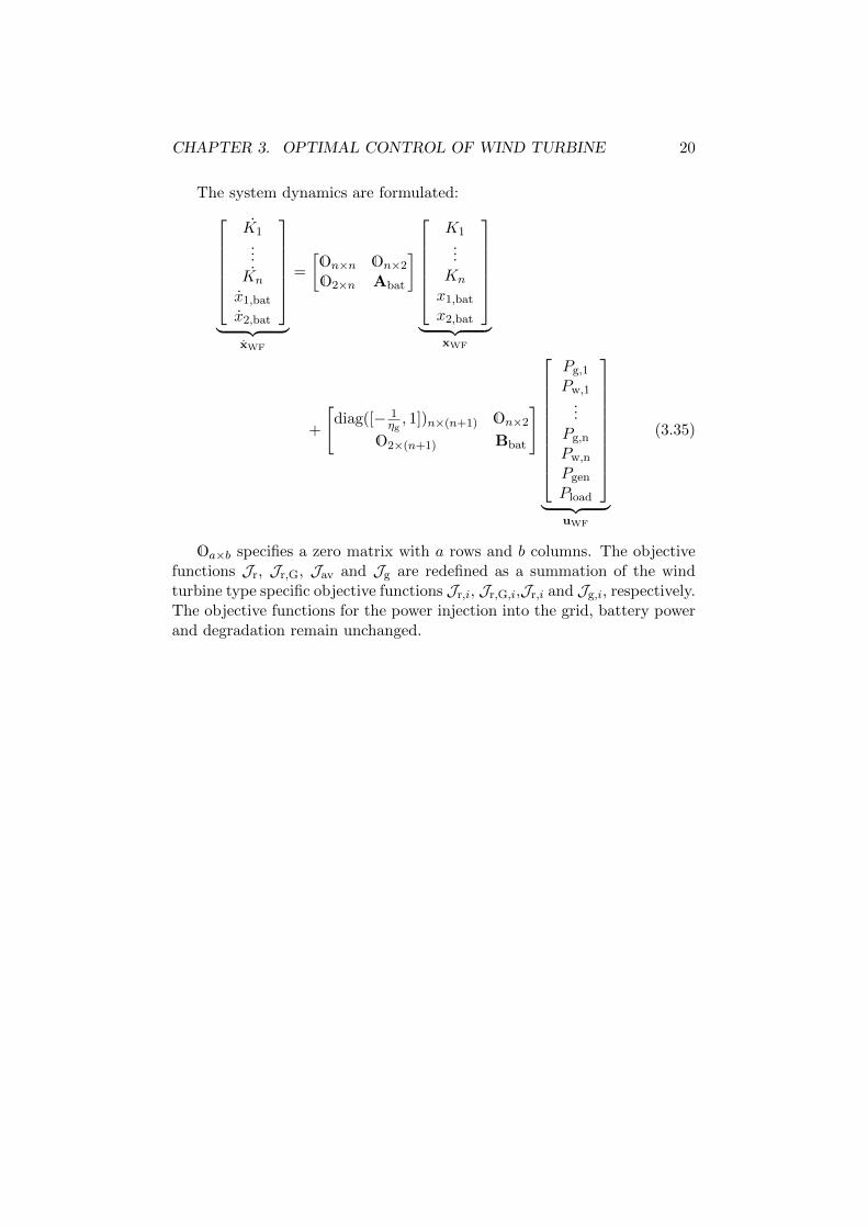
The system dynamics are formulated:K1...
Kn
x1,bat
x2,bat
︸ ︷︷ ︸
xWF
=
[On×n On×2
O2×n Abat
]
K1...Kn
x1,bat
x2,bat
︸ ︷︷ ︸
xWF
+
[diag([− 1
ηg, 1])n×(n+1) On×2
O2×(n+1) Bbat
]
Pg,1
Pw,1...
Pg,n
Pw,n
Pgen
Pload
︸ ︷︷ ︸
uWF
(3.35)
Oa×b specifies a zero matrix with a rows and b columns. The objectivefunctions Jr, Jr,G, Jav and Jg are redefined as a summation of the windturbine type specific objective functions Jr,i, Jr,G,i,Jr,i and Jg,i, respectively.The objective functions for the power injection into the grid, battery powerand degradation remain unchanged.
CHAPTER 3. OPTIMAL CONTROL OF WIND TURBINE 21
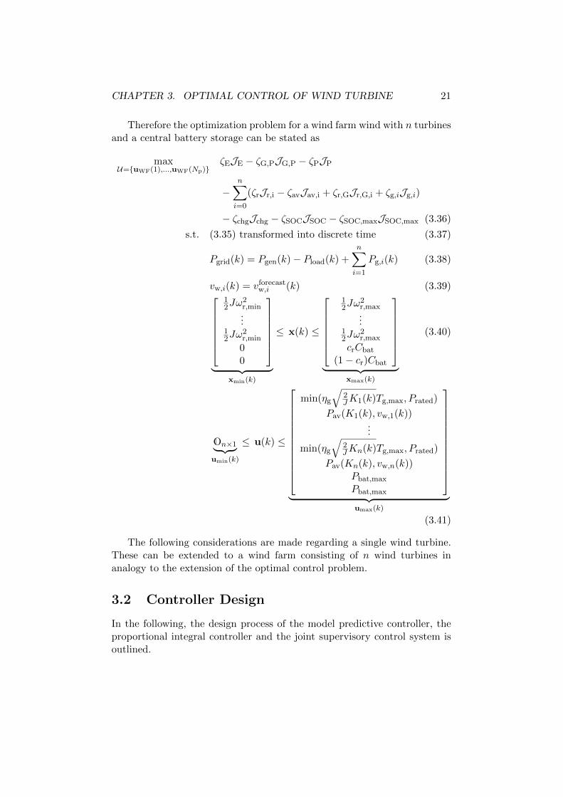
Therefore the optimization problem for a wind farm wind with n turbinesand a central battery storage can be stated as
maxU={uWF(1),...,uWF(Np)}
ζEJE − ζG,PJG,P − ζPJP
−n∑i=0
(ζrJr,i − ζavJav,i + ζr,GJr,G,i + ζg,iJg,i)
− ζchgJchg − ζSOCJSOC − ζSOC,maxJSOC,max (3.36)
s.t. (3.35) transformed into discrete time (3.37)
Pgrid(k) = Pgen(k)− Pload(k) +
n∑i=1
Pg,i(k) (3.38)
vw,i(k) = vforecastw,i (k) (3.39)
12Jω
2r,min...
12Jω
2r,min
00
︸ ︷︷ ︸
xmin(k)
≤ x(k) ≤
12Jω
2r,max...
12Jω
2r,max
crCbat
(1− cr)Cbat
︸ ︷︷ ︸
xmax(k)
(3.40)
On×1︸ ︷︷ ︸umin(k)
≤ u(k) ≤
min(ηg
√2JK1(k)Tg,max, Prated)
Pav(K1(k), vw,1(k))...
min(ηg
√2JKn(k)Tg,max, Prated)
Pav(Kn(k), vw,n(k))Pbat,max
Pbat,max
︸ ︷︷ ︸
umax(k)
(3.41)
The following considerations are made regarding a single wind turbine.These can be extended to a wind farm consisting of n wind turbines inanalogy to the extension of the optimal control problem.
3.2 Controller Design
In the following, the design process of the model predictive controller, theproportional integral controller and the joint supervisory control system isoutlined.
CHAPTER 3. OPTIMAL CONTROL OF WIND TURBINE 22
3.2.1 Model Predictive Control
A model predictive controller is designed which computes the optimal set-points for a system consisting of a wind turbine and an external batterystorage. The model predictive control entity uses the internal system model(3.27) to predict the system behavior. At every time step k the optimal se-quence of control inputs U = {u(1), . . . ,u(Np)} for a finite time horizon Np
is computed. For this purpose, the objective function in (3.26) is maximizedwhilst respecting constraints on state and control variables x,u. The firstentry in the optimal sequence u(1) is applied to the system. For the nexttime step the system states x and z are updated either by measurement orby using the internal model and the computation is repeated. This proce-dure is named receding horizon control. [31]
The wind velocity forecast can be obtained from statistical evaluation ofhistoric wind data or from a LiDAR measurement system mounted on thenacelle of a wind turbine. [32] gives an overview of wind speed predictiontechniques and [33] explains using continuous wave LIDAR for wind turbinecontrol.
3.2.2 Proportional Integral Control
In the control of the higher order wind turbine model formulated in Section2.2.1 a proportional integral (PI) controller is utilized. In general, a PIcontrol law can be written as
u(t) = Kpe(t) +Ki
∫ t
0e(τ)dτ , (3.42)
where u(t) is the control action, Kp the proportional and Ki the integralgain and e(t) is the control error [34]. The controller implemented in theAEOLUS SWF toolbox and designed for the NREL 5 MW wind turbine isdescribed by
βref = Kp∆ωg(t) +Ki
∫ t
0∆ωg(τ)dτ , (3.43)
where ∆ωg = ωg(t)− ωrefg is the deviation from a generator speed set point
which is stored in a look-up table and βref is the demanded pitch angle toachieve operation at an optimal set point [17].
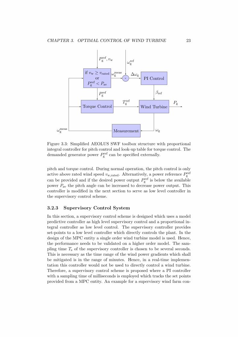
In Fig. 3.3, the control structure of the AEOLUS SWF toolbox is illus-trated. As introduced in Section 2.1, the generator torque Tg and the pitchangle β of the wind turbine are controlled. The pitch is regulated with thePI controller introduced in (3.43). The torque is controlled via a look-uptable. A measurement of the generator velocity ωmeas
g is provided for the
CHAPTER 3. OPTIMAL CONTROL OF WIND TURBINE 23
Torque Control Wind TurbineT ref
g
Measurement ωgωmeasg
PI Control
if vw ≥ vrated
orP ref
g < Pav
βref
Pg
-
ωrefg
P refg , vw
P refg
ωmeasg ∆ωg
Figure 3.3: Simplified AEOLUS SWF toolbox structure with proportionalintegral controller for pitch control and look-up table for torque control. Thedemanded generator power P ref
g can be specified externally.
pitch and torque control. During normal operation, the pitch control is onlyactive above rated wind speed vw,rated. Alternatively, a power reference P ref
g
can be provided and if the desired power output P refg is below the available
power Pav the pitch angle can be increased to decrease power output. Thiscontroller is modified in the next section to serve as low level controller inthe supervisory control scheme.
3.2.3 Supervisory Control System
In this section, a supervisory control scheme is designed which uses a modelpredictive controller as high level supervisory control and a proportional in-tegral controller as low level control. The supervisory controller providesset-points to a low level controller which directly controls the plant. In thedesign of the MPC entity a single order wind turbine model is used. Hence,the performance needs to be validated on a higher order model. The sam-pling time Ts of the supervisory controller is chosen to be several seconds.This is necessary as the time range of the wind power gradients which shallbe mitigated is in the range of minutes. Hence, in a real-time implemen-tation this controller would not be used to directly control a wind turbine.Therefore, a supervisory control scheme is proposed where a PI controllerwith a sampling time of milliseconds is employed which tracks the set pointsprovided from a MPC entity. An example for a supervisory wind farm con-
CHAPTER 3. OPTIMAL CONTROL OF WIND TURBINE 24
Torque Control Wind Turbine +
Battery
T refg
MPC
Measurement
vw,forecast
P refbat
P refg
Pg
vw
Pbat
Pgrid
PI Control
ωrefr
βref
Kmeas, Pmeasgrid
ωmeasg
ωmeasr
xmeasbat
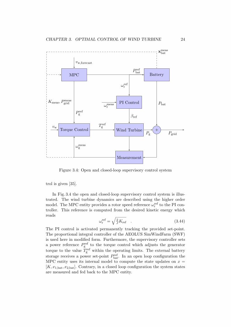
Figure 3.4: Open and closed-loop supervisory control system
trol is given [35].
In Fig. 3.4 the open and closed-loop supervisory control system is illus-trated. The wind turbine dynamics are described using the higher ordermodel. The MPC entity provides a rotor speed reference ωref
r to the PI con-troller. This reference is computed from the desired kinetic energy whichreads
ωrefr =
√2JKref . (3.44)
The PI control is activated permanently tracking the provided set-point.The proportional integral controller of the AEOLUS SimWindFarm (SWF)is used here in modified form. Furthermore, the supervisory controller setsa power reference P ref
g to the torque control which adjusts the generator
torque to the value T refg within the operating limits. The external battery
storage receives a power set-point P refbat. In an open loop configuration the
MPC entity uses its internal model to compute the state updates on x =[K,x1,bat, x2,bat]. Contrary, in a closed loop configuration the system statesare measured and fed back to the MPC entity.
Chapter 4
Implementation and Results
In this chapter, key findings regarding the implementation of the modelpredictive and the supervisory control scheme are presented. The benefitof incorporating kinetic and battery energy storage on the energy yield isinvestigated using a step response of the model predictive controller. Fur-thermore, the performance of the supervisory control system is examinedsubject to different wind scenarios. A variety of controller configurations iscompared to a benchmark regarding energy yield, power gradient and load-ing. The impact of the proposed control on the reduction of power gradientsis assessed in detail.
Perfect knowledge is assumed for the wind forecast that is used bythe supervisory control. The model predictive controller is implementedin MatLab R© [36] using YALMIP [37] for the formulation of the optimalcontrol problem. The optimization is solved in CPLEX R© [38].
4.1 Simulation Setup
4.1.1 Model Predictive Control
In the following, the model and control parameters are specified.
Table 4.1:Battery model specifications
ηgen 0.98 cw 0.1ηload 0.98 cr 0.5× 10⁻³
In Table 4.1 the parameters of the external battery storage are listed.Common lithium batteries have a energy-to-power (E/R) ratio of approxi-mately 1, which means that 1 kilowatt of battery power Pbat corresponds
25
CHAPTER 4. IMPLEMENTATION AND RESULTS 26
to 1 kilowatt-hour of battery capacity Cbat. A E/R ratio of 1 is thereforeassumed in the following simulations.
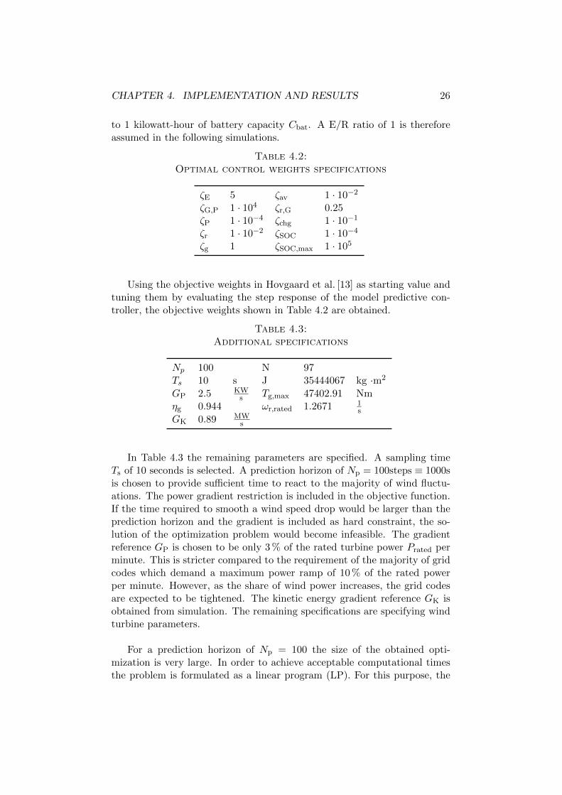
Table 4.2:Optimal control weights specifications
ζE 5 ζav 1 · 10−2
ζG,P 1 · 104 ζr,G 0.25ζP 1 · 10−4 ζchg 1 · 10−1
ζr 1 · 10−2 ζSOC 1 · 10−4
ζg 1 ζSOC,max 1 · 105
Using the objective weights in Hovgaard et al. [13] as starting value andtuning them by evaluating the step response of the model predictive con-troller, the objective weights shown in Table 4.2 are obtained.
Table 4.3:Additional specifications
Np 100 N 97Ts 10 s J 35444067 kg ·m2
GP 2.5 KWs Tg,max 47402.91 Nm
ηg 0.944 ωr,rated 1.2671 1s
GK 0.89 MWs
In Table 4.3 the remaining parameters are specified. A sampling timeTs of 10 seconds is selected. A prediction horizon of Np = 100steps ≡ 1000sis chosen to provide sufficient time to react to the majority of wind fluctu-ations. The power gradient restriction is included in the objective function.If the time required to smooth a wind speed drop would be larger than theprediction horizon and the gradient is included as hard constraint, the so-lution of the optimization problem would become infeasible. The gradientreference GP is chosen to be only 3 % of the rated turbine power Prated perminute. This is stricter compared to the requirement of the majority of gridcodes which demand a maximum power ramp of 10 % of the rated powerper minute. However, as the share of wind power increases, the grid codesare expected to be tightened. The kinetic energy gradient reference GK isobtained from simulation. The remaining specifications are specifying windturbine parameters.
For a prediction horizon of Np = 100 the size of the obtained opti-mization is very large. In order to achieve acceptable computational timesthe problem is formulated as a linear program (LP). For this purpose, the
CHAPTER 4. IMPLEMENTATION AND RESULTS 27
quadratic penalty on power variation in the objective function (3.14) and theconstraint on the generator power in (3.4) are approximated by piece-wiselinear functions. As a result, for a sampling time Ts of 10 seconds the modelpredictive controller uses 10 to 20 seconds of computational time for onetime step, which should be further reduced for a real-time application. Fora wind farm consisting of several wind turbines, the optimization problembecomes larger thus the computational effort increases.
4.1.2 Supervisory Control System
In the following, the implementation of the supervisory control scheme in-troduced in Section 3.2.3 is outlined. The key finding is that the output ofthe high level MPC entity has to be post-processed to be used as a set-pointωref
r for the low level PI controller. The main reasons are the introducedmodel approximations in the optimal control formulation and that the lowlevel controller cannot directly regulate the kinetic energy variation.
In the single order wind turbine model, the ramp of the kinetic energyis solely determined by the imbalance between generator power Pw and ex-tracted wind power Pg. The MPC directly controls the variation of kineticenergy K by setting the appropriate values for the control variables Pw andPg. Contrary, the low level wind turbine control can influence the kineticenergy either by changing the blade pitch angle β or by adjusting the gen-erator torque Tg. The blade pitch β regulates the extracted wind power Pw
and the generator torque Tg the generator power Pg. The rotational velocityof rotor ωr and generator shaft ωg are coupled via the drive-train dynamics.
In order to increase kinetic energy, the pitch angle is decreased to extractmore power. Kinetic energy is reduced when the generator demands morepower than is extracted from the wind. The generator power can be influ-enced by adjusting the generator torque. During kinetic energy extraction,it is crucial that the PI controller avoids increasing the pitch angle to fulfilla desired trajectory of the rotational velocity. Otherwise, the kinetic energyis lost and cannot be provided to the generator.
In the higher order model, a third-order model describes the drive-traindynamics. During simulation studies, it is revealed that especially duringkinetic energy extraction, model mismatch between the single order and thehigher order model is present. This mismatch leads to kinetic energy notbeing sufficiently provided to fulfill the desired output power trajectory. Itis therefore necessary to post-process the output of the model predictivecontroller before using it as an input for the PI control.
CHAPTER 4. IMPLEMENTATION AND RESULTS 28
0 50 100 150 200
1.2
1.4
1.6
1.8
2
Time [10s]
Rota
tion
alsp
eed
refe
ren
ceω
ref
r[1 s
]
1st mod.
2nd mod.
3rd mod.initial
Figure 4.1: Reference trajectory for rotational wind speed ωrefr and the three
modifications applied to the trajectory. The wind step is from 12 ms to 10 m
s .(Np = 200)
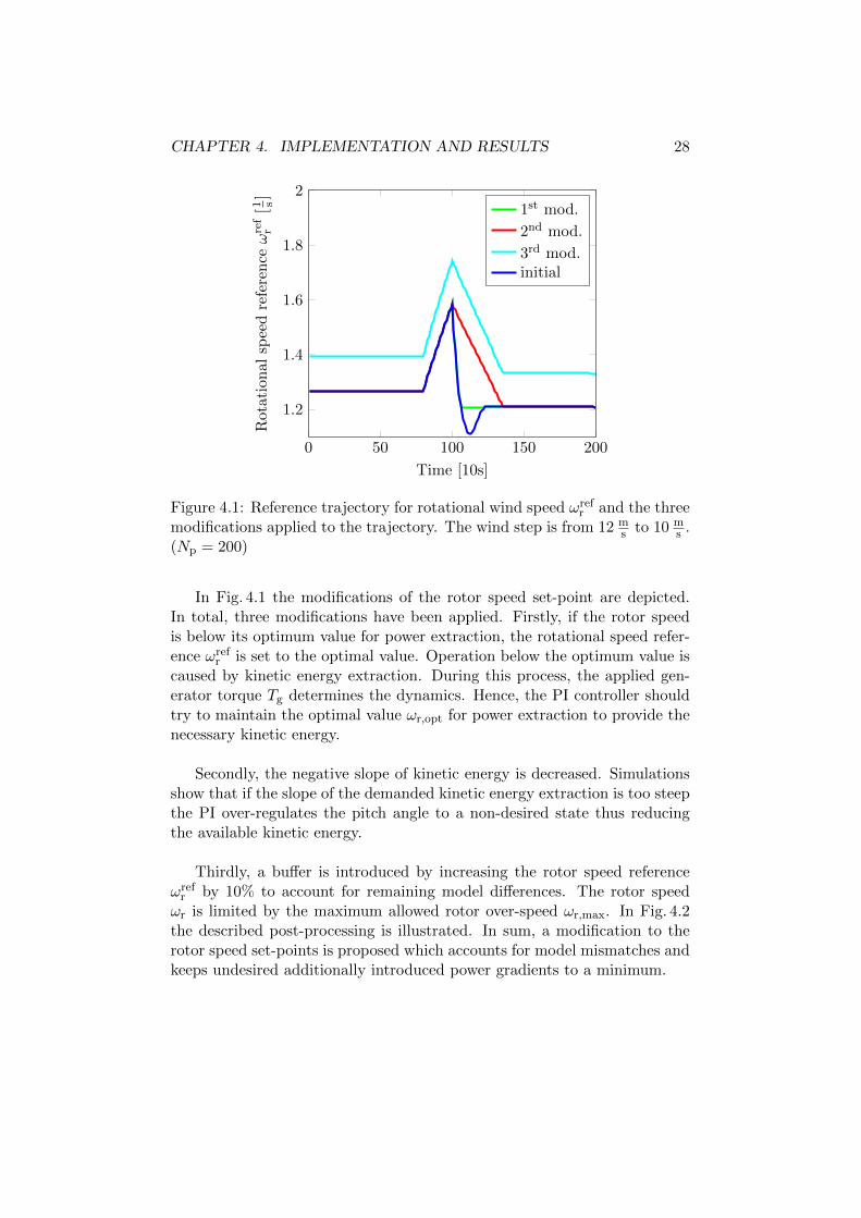
In Fig. 4.1 the modifications of the rotor speed set-point are depicted.In total, three modifications have been applied. Firstly, if the rotor speedis below its optimum value for power extraction, the rotational speed refer-ence ωref
r is set to the optimal value. Operation below the optimum value iscaused by kinetic energy extraction. During this process, the applied gen-erator torque Tg determines the dynamics. Hence, the PI controller shouldtry to maintain the optimal value ωr,opt for power extraction to provide thenecessary kinetic energy.
Secondly, the negative slope of kinetic energy is decreased. Simulationsshow that if the slope of the demanded kinetic energy extraction is too steepthe PI over-regulates the pitch angle to a non-desired state thus reducingthe available kinetic energy.
Thirdly, a buffer is introduced by increasing the rotor speed referenceωref
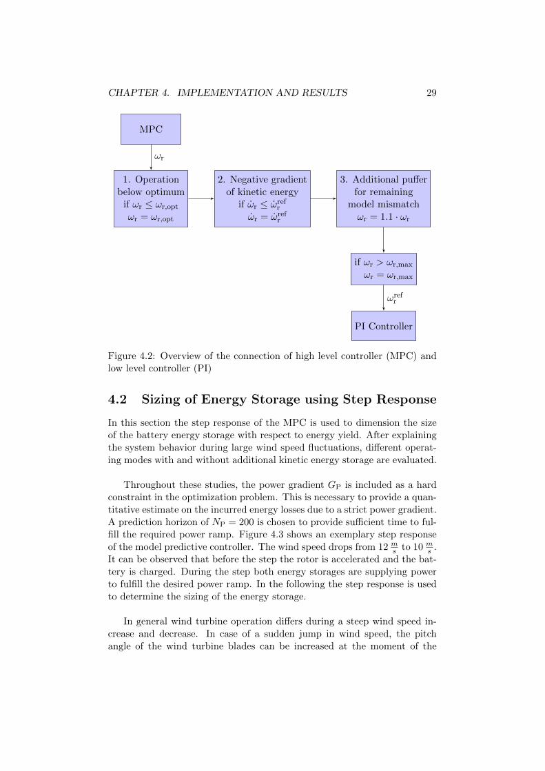
r by 10% to account for remaining model differences. The rotor speedωr is limited by the maximum allowed rotor over-speed ωr,max. In Fig. 4.2the described post-processing is illustrated. In sum, a modification to therotor speed set-points is proposed which accounts for model mismatches andkeeps undesired additionally introduced power gradients to a minimum.
CHAPTER 4. IMPLEMENTATION AND RESULTS 29
MPC
1. Operationbelow optimum
if ωr ≤ ωr,opt
ωr = ωr,opt
2. Negative gradientof kinetic energy
if ωr ≤ ωrefr
ωr = ωrefr
3. Additional pufferfor remaining
model mismatchωr = 1.1 · ωr
if ωr > ωr,max
ωr = ωr,max
PI Controller
ωr
ωrefr
Figure 4.2: Overview of the connection of high level controller (MPC) andlow level controller (PI)
4.2 Sizing of Energy Storage using Step Response
In this section the step response of the MPC is used to dimension the sizeof the battery energy storage with respect to energy yield. After explainingthe system behavior during large wind speed fluctuations, different operat-ing modes with and without additional kinetic energy storage are evaluated.
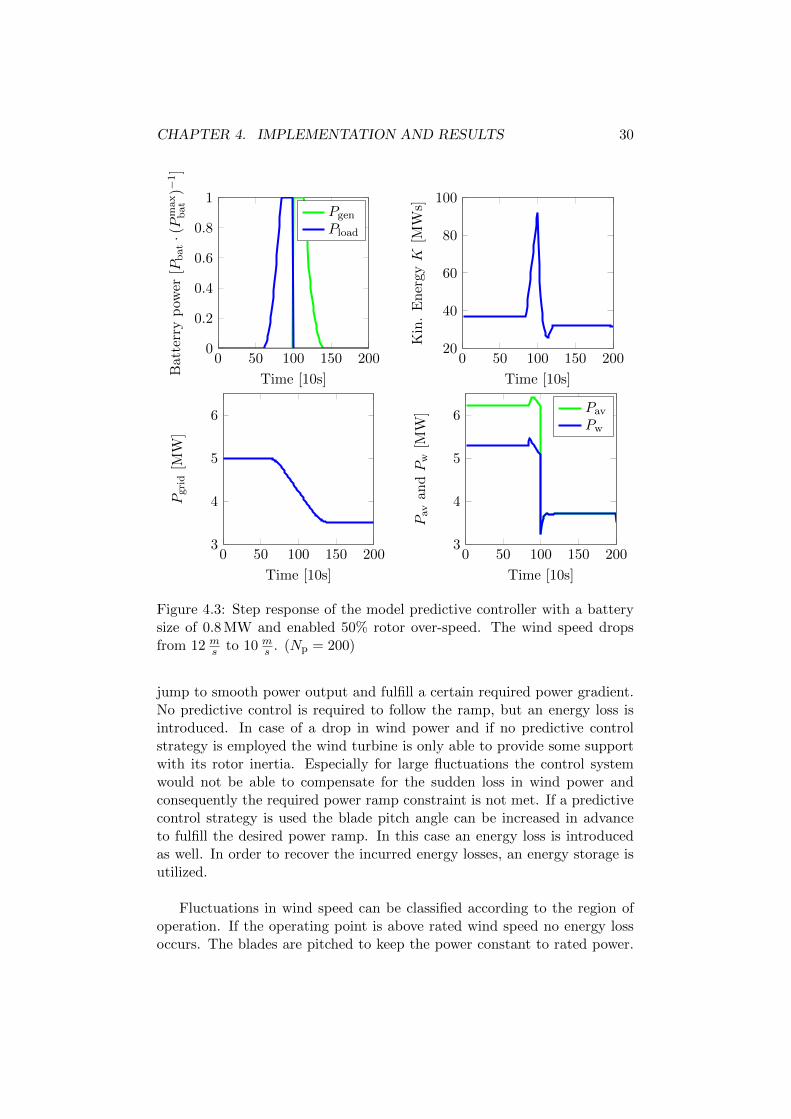
Throughout these studies, the power gradient GP is included as a hardconstraint in the optimization problem. This is necessary to provide a quan-titative estimate on the incurred energy losses due to a strict power gradient.A prediction horizon of NP = 200 is chosen to provide sufficient time to ful-fill the required power ramp. Figure 4.3 shows an exemplary step responseof the model predictive controller. The wind speed drops from 12 m
s to 10 ms .
It can be observed that before the step the rotor is accelerated and the bat-tery is charged. During the step both energy storages are supplying powerto fulfill the desired power ramp. In the following the step response is usedto determine the sizing of the energy storage.
In general wind turbine operation differs during a steep wind speed in-crease and decrease. In case of a sudden jump in wind speed, the pitchangle of the wind turbine blades can be increased at the moment of the
CHAPTER 4. IMPLEMENTATION AND RESULTS 30
0 50 100 150 2000
0.2
0.4
0.6
0.8
1
Time [10s]
Bat
terr
yp
ower
[Pb
at·(P
max
bat
)−1]
Pgen
Pload
0 50 100 150 20020
40
60
80
100
Time [10s]
Kin
.E
ner
gyK
[MW
s]
0 50 100 150 2003
4
5
6
Time [10s]
Pgri
d[M
W]
0 50 100 150 2003
4
5
6
Time [10s]
Pav
andP
w[M
W] Pav
Pw
Figure 4.3: Step response of the model predictive controller with a batterysize of 0.8 MW and enabled 50% rotor over-speed. The wind speed dropsfrom 12 m
s to 10 ms . (Np = 200)
jump to smooth power output and fulfill a certain required power gradient.No predictive control is required to follow the ramp, but an energy loss isintroduced. In case of a drop in wind power and if no predictive controlstrategy is employed the wind turbine is only able to provide some supportwith its rotor inertia. Especially for large fluctuations the control systemwould not be able to compensate for the sudden loss in wind power andconsequently the required power ramp constraint is not met. If a predictivecontrol strategy is used the blade pitch angle can be increased in advanceto fulfill the desired power ramp. In this case an energy loss is introducedas well. In order to recover the incurred energy losses, an energy storage isutilized.
Fluctuations in wind speed can be classified according to the region ofoperation. If the operating point is above rated wind speed no energy lossoccurs. The blades are pitched to keep the power constant to rated power.
CHAPTER 4. IMPLEMENTATION AND RESULTS 31
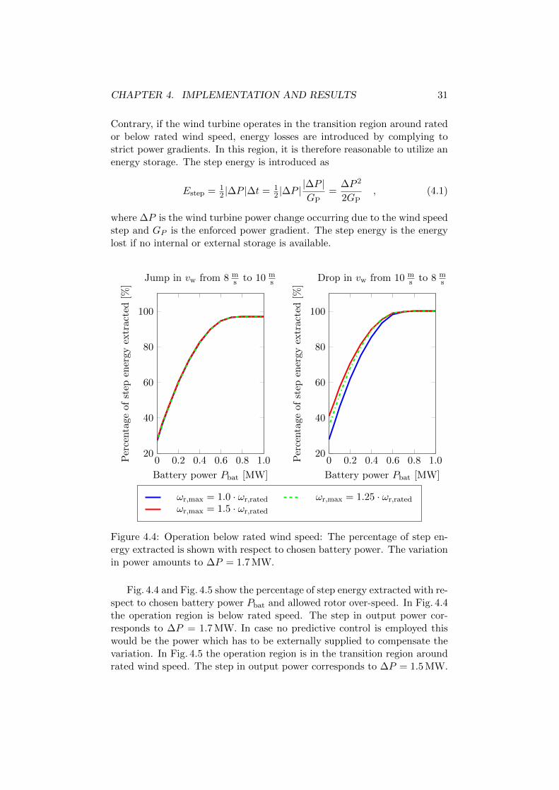
Contrary, if the wind turbine operates in the transition region around ratedor below rated wind speed, energy losses are introduced by complying tostrict power gradients. In this region, it is therefore reasonable to utilize anenergy storage. The step energy is introduced as
Estep = 12 |∆P |∆t = 1
2 |∆P ||∆P |GP
=∆P 2
2GP, (4.1)
where ∆P is the wind turbine power change occurring due to the wind speedstep and GP is the enforced power gradient. The step energy is the energylost if no internal or external storage is available.
20
40
60
80
100
0 0.2 0.4 0.6 0.8 1.0
Battery power Pbat [MW]
Per
centa
geof
step
ener
gyex
tract
ed[%
]
Jump in vw from 8 ms to 10 m
s
20
40
60
80
100
0 0.2 0.4 0.6 0.8 1.0
Battery power Pbat [MW]
Per
centa
geof
step
ener
gyex
trac
ted
[%]
Drop in vw from 10 ms to 8 m
s
ωr,max = 1.0 · ωr,rated ωr,max = 1.25 · ωr,rated
ωr,max = 1.5 · ωr,rated
Figure 4.4: Operation below rated wind speed: The percentage of step en-ergy extracted is shown with respect to chosen battery power. The variationin power amounts to ∆P = 1.7 MW.
Fig. 4.4 and Fig. 4.5 show the percentage of step energy extracted with re-spect to chosen battery power Pbat and allowed rotor over-speed. In Fig. 4.4the operation region is below rated speed. The step in output power cor-responds to ∆P = 1.7 MW. In case no predictive control is employed thiswould be the power which has to be externally supplied to compensate thevariation. In Fig. 4.5 the operation region is in the transition region aroundrated wind speed. The step in output power corresponds to ∆P = 1.5 MW.
CHAPTER 4. IMPLEMENTATION AND RESULTS 32
20
40
60
80
100
0 0.2 0.4 0.6 0.8 1.0
Battery power Pbat [MW]
Per
centa
ge
ofst
epen
ergy
extr
acte
d[%
]
Jump in vw from 10 ms to 12 m
s
20
40
60
80
100
0 0.2 0.4 0.6 0.8 1.0
Battery power Pbat [MW]
Per
centa
ge
of
step
ener
gyex
trac
ted
[%]
Drop in vw from 12 ms to 10 m
s
ωr,max = 1.0 · ωr,rated ωr,max = 1.25 · ωr,rated
ωr,max = 1.5 · ωr,rated
Figure 4.5: Operation in the transition region around rated wind speed: Thepercentage of step energy extracted is shown with respect to chosen batterypower. The variation in power amounts to ∆P = 1.5 MW.
In both scenarios three configurations of rotor speed are specified: no rotorover-speed, 25% rotor over-speed and 50% rotor over-speed. Several obser-vations for both operating regimes are outlined in the following.
In case of a jump in wind speed, enabling rotor over-speed does not in-crease the energy yield. The wind turbine already extracts maximum powerbefore the wind step and thus cannot extract surplus power to increase therotational speed. For both configurations the system can extract around30% of the step energy for a jump in wind speed. This is done by using thekinetic energy to smooth the power fluctuation during the step. By addingan external battery energy storage the energy yield can be increased. In theoperation below rated wind speed a linear increase from 30% to approxi-mately 70% of extracted step energy with a battery power of 0.3 MW canbe observed. If the battery power is further increased, the slope decreasessaturating at a value close to 100% with a battery power of 0.8 MW. In thiscase, it is not possible to reach 100% as losses in the battery storage areincurred. Similar behavior is observed for operation in the transition regionaround rated wind speed. As the power variation ∆P = 1.5 MW is smallerthan the one before ∆P = 1.7 MW, less battery power is required. Hence,
CHAPTER 4. IMPLEMENTATION AND RESULTS 33
with a battery power of 0.3 MW around 80% of the step energy can be ex-tracted.
In case of a drop in wind speed enabling 25% and 50% rotor over-speedyields an increase in energy capture. For Fig. 4.4, an increase from 28% over36% to 41% can be observed and in Fig. 4.5 an increase from 21% over 36%to 44%. In operation below rated wind speed the surplus step energy ex-tracted by allowing rotor over-speed decreases with increasing battery sizeuntil the step energy yields saturates at 100%. Above a battery power of0.6 MW the impact of rotor over-speed on step energy yield is negligible.This is due to the fact that no surplus energy can be extracted as the tur-bine already extracts the maximum wind power. Contrary, in the operationin the transition region around rated wind speed, the wind turbine can ex-tract additional surplus energy. In Fig. 4.5, without rotational over-speed99.5% of of step energy can be extracted, with 25% rotor over-speed 102%and with 50% rotor over-speed 105%, respectively. In this case the benefitof incorporating kinetic energy with rotor over-speed is apparent. Withoutrotor over-speed a battery of 0.7 MW has to be used to yield 99% of the stepenergy. With 50% rotor over-speed it is only necessary to use a battery sizeof 0.45 MW.
This behavior is similarly exhibited for different wind step sizes. Thecurves are only shifted horizontally depending on the magnitude of the powervariation ∆P . The main findings are the following. Additional external stor-age increases the energy yield approximately linear followed by a saturationphase up to 100%. In case of a wind speed drop, utilizing kinetic energy canincrease energy yield. In particular if the wind turbine operates above ratedwind speed before a substantial decrease in wind speed, additional surplusenergy can be extracted. Consequently, these results indicate that rotorover-speed allows to reduce the battery size while the same energy yield isobtained.
4.3 Performance of Designed Controllers under Dif-ferent Wind Scenarios
In this section, the performance of the proposed control schemes is evalu-ated. In particular, the supervisory control system which comprises a PIcontroller and a MPC entity is subject to several wind scenarios. Energyyield, mitigation of power gradients and loading on the turbine are exam-ined. Furthermore, this section serves as validation of the model predictivecontrol on a higher order model.

CHAPTER 4. IMPLEMENTATION AND RESULTS 34
The setup of the simulations is explained in the following. The PI con-troller of the AEOLUS SWF toolbox is used as benchmark. The super-visory control is implemented as open-loop control as described in Section3.2.3. For a given wind scenario the MPC entity pre-computes the optimalset-points for power and rotational velocity (P ref
g ,ωrefr ). The wind turbine
set-points are used as an input to a PI controller and a torque control basedon the AEOLUS SWF toolbox. The battery receives a set point P ref
bat fromthe MPC. The sampling time of both PI controller is set to 0.0125 s as pro-posed in [18]. For constructing the wind time histories, 1-min averaged winddata from the National Wind Technology Center (NWTC) M2 tower belong-ing to the National Renewable Energy Laboratory is used [39]. With thestochastic, full-field, turbulence simulator TurbSim [40] 10 seconds fill-insare created for the 1-min wind data. Three different hourly wind scenariosare selected from the provided mast data. For evaluating the results, thefirst 100 seconds are omitted to account for the ramping up of the controllaws.
CHAPTER 4. IMPLEMENTATION AND RESULTS 35
5
10
15
0 500 1000 1500 2000 2500 3000 3500
Time [s]
Win
dS
pee
d[m s
]
0 500 1000 1500 2000 2500 3000 35000
2
4
6
Time [s]
Pow
er[M
W]
PI benchmark Supervisory control system
0 500 1000 1500 2000 2500 3000 3500
0
2
4
6
Time [s]
Pow
er[M
W]
Pgrid Pg Pbat
0 500 1000 1500 2000 2500 3000 3500
0
2
4
6
Time [s]
Pow
er[M
W]
Supervisory control system Pg MPC reference P refg
Error
Figure 4.6: The output of the supervisory control system (rotor over-speedenabled and Pbat = 0.8MW) is compared to the benchmark PI controllerand to the reference provided by the MPC controller.
CHAPTER 4. IMPLEMENTATION AND RESULTS 36
In Fig. 4.6 the response of the low level controller with set-points pro-vided from the MPC entity (rotor over-speed enabled ωr,max = 1.5ωr,rated
and Pbat = 0.8 MW) is shown for an exemplary wind scenario. The powerinjection Pgrid is compared to the benchmark PI controller. The proposedcontrol scheme is able to inject a substantially smoother power into the grid.The power in-feed to the grid Pgrid consists of the generator power Pg andthe battery power Pbat. Both are controlled via MPC set-points P ref
g and
P refbat, respectively. A small error between the demanded generator powerP ref
g and the generator power Pg is observed.
0 500 1000 1500 2000 2500 3000 35000
20
40
60
80
Time [s]
Kin
etic
Ener
gyK
[MW
s]
Supervisory control system MPC reference unmodifiedMPC reference modified
Figure 4.7: Kinetic energy compared between the supervisory control system(rotor over-speed enabled and Pbat = 0.8 MW) and the unmodified andmodified kinetic energy reference provided to the PI controller
CHAPTER 4. IMPLEMENTATION AND RESULTS 37
0
0.1
0.2
0.3
0.4
0 500 1000 1500 2000 2500 3000 3500
Time [s]
Bat
tery
state
sx
bat
[MW
h]
battery charge well x1,bat Battery charge well x2,bat
Figure 4.8: Battery states xbat = [x1,bat, x2,bat]> for the supervisory control
system (rotor over-speed enabled and Pbat = 0.8 MW)
For the same configuration, in Fig. 4.7 the kinetic energy is depicted. Inaddition, the unmodified and modified kinetic energy reference is provided.The unmodified trajectory is the one predicted by the model predictive con-troller. The modified trajectory accounts for the deviations between singleand higher order wind turbine model and is described in Section 4.1.2. Itcan be observed that during large extractions of kinetic energy, when thegenerator extracts more power than the rotor provides, the kinetic energytrajectory from the PI controller mimics the predicted one by the MPC en-tity. During normal modes of operation a certain offset of kinetic energycan be observed. This highlights the challenge of efficiently incorporatingthe MPC reference into the higher order wind turbine model with the lowlevel controller.
Finally, Fig. 4.8 depicts the states of the battery capacity xbat. We canobserve that the first charge well x1,bat is primarily utilized.
In the next step, the performance of a range of configurations for thesupervisory control scheme is quantitatively evaluated and compared to astandard PI benchmark controller. Certain indicators are considered toevaluate the performance. The actuator duty cycle (ADC) is defined as
ADC =1
Tfinal − Tinitial
∫ Tfinal
Tinitial
βdt , (4.2)
CHAPTER 4. IMPLEMENTATION AND RESULTS 38
where the observation time is ranging from Tinitial to Tfinal and β is thederivative of the pitch angle β. A higher actuator duty cycle resembles anincrease in pitching activity and consequently an increased wear on pitch-ing actuators. The damage equivalent load (DEL) for the torsion momentof the rotor shaft and the tower root bending moment are computed withthe AEOLUS SWF toolbox using a rainflow-counting method. The detailedprocedure is described in [41] and [42]. In order to evaluate the power gradi-ents, the average gradient over a time step of 10 seconds is computed. Themaximum absolute power gradient is evaluated and the standard deviationof the gradients is computed.
In Table 4.4, energy yield, actuator duty cycle, power gradients and dam-age equivalent loads are compared to a benchmark PI controller. The actua-tor duty cycle increases slightly for the proposed supervisory control scheme.This is due to pitch activity being enabled throughout the whole operatingregion, not only in the region above rated wind speed. The energy loss in-curred by obeying a tight power gradient accounts to 27.4% without rotorover-speed and without external battery storage. By allowing 50% rotorover-speed, additional 5.0% energy can be extracted. With a battery powerof 0.5 MW, additional 11.2% energy can be recovered. If a battery with1 MW power is employed, the energy yield amounts to 97.0% compared tothe benchmark controller. The remaining 3.0% of energy are not recovereddue to losses in the battery system and sub-optimal wind turbine operation.The DEL of the tower root bending moment increases if rotor over-speed isenabled. Without battery storage the damage equivalent load increases by30% compared to the benchmark PI controller. Using a battery with 1 MWpower the increase amounts to 20% as less kinetic energy has to be utilizedto fulfill the power ramp restrictions. For the torsion moment of the rotorshaft a decrease in the damage equivalent load is observed. Using a batterywith 1 MW power the decrease amounts to 4.5%.
The proposed supervisory control substantially mitigates power gradi-ents. The maximum absolute power gradient is reduced by roughly twothirds for the majority of configurations. The standard deviation is reducedby approximately one order of magnitude. Power gradients are further atten-uated with increasing storage size. If no external battery storage is employedthe maximum absolute gradient and the standard deviation is reduced by61.9% and 84.1%, respectively. Using a battery with 1 MW power the powergradients can be further reduced and the maximum absolute gradient andthe standard deviation amount to 78.5% and 88.7% of the benchmark value,respectively. For the configuration with enabled rotor over-speed and batterypower of 1 MW the power gradients are compared in Fig. 4.9 in a histogram.The observation confirms that the power gradients are substantially reducedfor all three wind scenarios.
CHAPTER 4. IMPLEMENTATION AND RESULTS 39
Table4.4:
ADC,energyyield,powergradientsand
DELsfordifferentconfigurations
Con
figura
tions
AB
CD
EF
Bat
tery
pow
erP
bat[
MW
]P
IB
ench
mar
koff
off0.
250.
51.
0M
axim
um
roto
rov
er-s
pee
dω
r,m
ax
ωra
ted
ωra
ted
1.5ω
rate
d1.5ω
rate
d1.
5ω
rate
d1.5ω
rate
d
Act
uato
rd
uty
cycl
e[1 s
]0.
180.
220.
220.
220.
220.
23E
ner
gy
yie
ld[%
]10
0.0
72.6
77.6
83.3
88.8
97.0
Pow
ergr
adie
nt
(MA
X)
[kW s
]19
0.7
77.1
53.5
53.7
54.7
41.0
Pow
ergr
adie
nt
(ST
D)
[kW s
]43
.57.
86.
96.
96.
54.
9T
ower
root
ben
din
g57
.352
.474
.572
.973
.669
.3m
omen
t(D
EL
)[M
Nm
,%]
100.
091
.413
0.0
127.
212
8.4
120.
9T
ors
ion
mom
ent
of
the
3.17
2.54
2.63
2.76
2.78
3.01
roto
rsh
aft
(DE
L)
[MN
m,%
]10
0.0
80.5
83.2
87.4
88.2
95.5
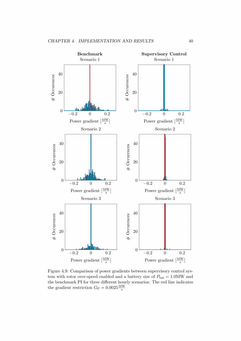
CHAPTER 4. IMPLEMENTATION AND RESULTS 40
−0.2 0 0.20
20
40
Power gradient [MWs ]
#O
ccure
nce
sBenchmark
Scenario 1
−0.2 0 0.20
20
40
Power gradient [MWs ]
#O
ccure
nce
s
Supervisory ControlScenario 1
−0.2 0 0.20
20
40
Power gradient [MWs ]
#O
ccure
nce
s
Scenario 2
−0.2 0 0.20
20
40
Power gradient [MWs ]
#O
ccure
nce
sScenario 2
−0.2 0 0.20
20
40
Power gradient [MWs ]
#O
ccure
nce
s
Scenario 3
−0.2 0 0.20
20
40
Power gradient [MWs ]
#O
ccure
nce
s
Scenario 3
Figure 4.9: Comparison of power gradients between supervisory control sys-tem with rotor over-speed enabled and a battery size of Pbat = 1.0MW andthe benchmark PI for three different hourly scenarios: The red line indicatesthe gradient restriction GP = 0.0025MW
s
Chapter 5
Conclusion
5.1 Summary of Results
In this thesis a supervisory control system is developed which is able to sub-stantially mitigate power gradients in wind energy system operation. Forthis purpose, the kinetic energy stored in the rotor inertia is utilized and anexternal battery energy storage is employed. A model predictive controllerserves as supervisory controller providing set-points for torque, pitch andbattery control. The pitch angle is regulated by a PI controller.
An existing optimal control formulation is further extended includinga battery model capturing fast transient battery dynamics and a batterydegradation objective. Using the step response of the MPC, an estimate onenergy yield in dependence on battery storage size and allowed maximumrotor-speed is provided. As model mismatches between the high and lowlevel controller are present, appropriate modifications to the set-points arepresented. The supervisory control system is subject to different wind sce-narios and an analysis regarding energy yield, power gradients and loadingon the turbine is provided. It is found that if the battery power is 20% ofthe rated wind turbine power and the maximum allowable rotor speed is 1.5times the rated speed, the energy yield amounts to 97.0% compared to astandard PI controller. The maximum power gradient is reduced by 78.5%and the standard deviation by 88.7%. The DEL of the tower root bend-ing moment increased moderately by 20% and for the DEL of the torsionmoment of the rotor shaft we observe a slight decrease by 4.5%. Hence,the proposed control is able to comply with tight power ramp restrictionswhile keeping energy losses and the increase in turbine loading to a mini-mum. Utilizing an external battery storage substantially increases energyyield and further reduces power gradients and tower loading.
41

CHAPTER 5. CONCLUSION 42
5.2 Outlook
In the following, an outlook on further extensions is given. The next stepin the controller design process is to evaluate the performance on an aeroe-lastic wind turbine simulator using realistic wind data with sampling timeof milliseconds. The loading due to rotor over-speed in particular on theblades could be further investigated. In this thesis, perfect knowledge offuture wind speed is assumed for the forecast used by the model predictivecontroller. Light Detection And Ranging (LiDAR) or statistical approachesfor wind speed forecasting could be incorporated. In literature spatial av-eraging effects in wind farms are reported reducing the necessity of windpower smoothing. These could also be included in the supervisory controlformulation.
Bibliography
[1] Global Wind Energy Council. Global wind 2014 report. Global WindEnergy Council, Brussels, Belgium, 2015.
[2] Scott Valentine. Wind Power Politics and Policy. Oxford UniversityPress, 2014.
[3] Lars Christian Henriksen. Model predictive control of a wind turbine.PhD thesis, Technical University of Denmark, DTU, DK-2800 Kgs. Lyn-gby, Denmark, 2007.
[4] Wai Hall Lio, JA Rossiter, and Bryn L Jones. A review on applicationsof model predictive control to wind turbines. In Control (CONTROL),2014 UKACC International Conference on, pages 673–678. IEEE, 2014.
[5] D-I Stroe, A-I Stan, Robert Diosi, Remus Teodorescu, and Søren JuhlAndreasen. Short term energy storage for grid support in wind powerapplications. In Optimization of Electrical and Electronic Equipment(OPTIM), 2012 13th International Conference on, pages 1012–1021.IEEE, 2012.
[6] Ted KA Brekken, Alex Yokochi, Annette Von Jouanne, Zuan Z Yen,Hannes Max Hapke, and Douglas A Halamay. Optimal energy storagesizing and control for wind power applications. Sustainable Energy,IEEE Transactions on, 2(1):69–77, 2011.
[7] Francisco Dıaz-Gonzalez, Andreas Sumper, Oriol Gomis-Bellmunt, andRoberto Villafafila-Robles. A review of energy storage technologies forwind power applications. Renewable and Sustainable Energy Reviews,16(4):2154–2171, 2012.
[8] Simon De Rijcke, Johan Meyers, and Johan Driesen. Reducing powergradients in large-scale wind farms by optimal active power control. InPowerTech (POWERTECH), 2013 IEEE Grenoble, pages 1–6. IEEE,2013.
[9] Simon De Rijcke, Johan Driesen, and Johan Meyers. Power smoothingin large wind farms using optimal control of rotating kinetic energyreserves. Wind Energy, 2014.
43
BIBLIOGRAPHY 44
[10] Philip Clemow, Timothy C Green, and Carlos A Hernandez-Aramburo.Wind farm output smoothing through co-ordinated control and short-term wind speed prediction. In Proc. IEEE Int. Conf. Power and En-ergy Society General Meeting, pages 1–8, 2010.
[11] Le Xie, Yingzhong Gu, Ali Eskandari, and Mehrdad Ehsani. Fast mpc-based coordination of wind power and battery energy storage systems.Journal of Energy Engineering, 138(2):43–53, 2012.
[12] Tobias Gybel Hovgaard, Lars FS Larsen, JB Jorgensen, and StephenBoyd. Mpc for wind power gradients - utilizing forecasts, rotor iner-tia, and central energy storage. In Control Conference (ECC), 2013European, pages 4071–4076. IEEE, 2013.
[13] Tobias Gybel Hovgaard, Stephen Boyd, and John Bagterp Jørgensen.Model predictive control for wind power gradients. Wind Energy, 2014.
[14] Constantinos Sourkounis and Pavlos Tourou. Grid code requirementsfor wind power integration in europe. In Conference Papers in Science,volume 2013. Hindawi Publishing Corporation, 2013.
[15] Marina Tsili and S Papathanassiou. A review of grid code techni-cal requirements for wind farms. IET Renewable Power Generation,3(3):308–332, 2009.
[16] Thomas Ackermann et al. Wind power in power systems, volume 140.Wiley Online Library, 2005.
[17] Jason Mark Jonkman, Sandy Butterfield, Walter Musial, and GeorgeScott. Definition of a 5-MW reference wind turbine for offshore sys-tem development. National Renewable Energy Laboratory Golden, CO,2009.
[18] Jacob Deleuran Grunnet, Mohsen Soltani, Torben Knudsen, Martin Ny-gaard Kragelund, and Thomas Bak. Aeolus toolbox for dynamics windfarm model, simulation and control. In The European Wind EnergyConference & Exhibition, EWEC 2010, 2010.
[19] Tony Burton, David Sharpe, Nick Jenkins, and Ervin Bossanyi. Windenergy handbook. John Wiley & Sons, 2001.
[20] P Sørensen, AD Hansen, F Iov, and F Blaabjerg. Modeling of wind farmcontrollers. In 2006 European Wind Energy Conference and Exhibition,2006.
[21] James F Manwell, Jon G McGowan, and Anthony L Rogers. Windenergy explained: theory, design and application. John Wiley & Sons,2010.
BIBLIOGRAPHY 45
[22] Alexandre Teninge, Cristian Jecu, Daniel Roye, Seddik Bacha, JeromeDuval, and Regine Belhomme. Contribution to frequency controlthrough wind turbine inertial energy storage. IET Renewable PowerGeneration, 3(3):358–370, 2009.
[23] Jacob Aho, Andrew Buckspan, Jason Laks, Paul Fleming, Yunho Jeong,Fiona Dunne, Matthew Churchfield, Lucy Pao, and Kathryn Johnson.A tutorial of wind turbine control for supporting grid frequency throughactive power control. In American Control Conference (ACC), 2012,pages 3120–3131. IEEE, 2012.
[24] Sadegh Ghani Varzaneh, GB Gharehpetian, and Mehrdad Abedi. Out-put power smoothing of variable speed wind farms using rotor-inertia.Electric Power Systems Research, 116:208–217, 2014.
[25] T Knuppel, Jørgen Nygard Nielsen, Kim Høj Jensen, Andrew Dixon,and J Otergaard. Power oscillation damping controller for wind powerplant utilizing wind turbine inertia as energy storage. In Power andEnergy Society General Meeting, 2011 IEEE, pages 1–8. IEEE, 2011.
[26] German Claudio Tarnowski, PC Kjar, PE Sorensen, and J Ostergaard.Variable speed wind turbines capability for temporary over-production.In Power & Energy Society General Meeting, 2009. PES’09. IEEE,pages 1–7. IEEE, 2009.
[27] Barry Rawn and Peter Lehn. Wind rotor inertia and variable efficiency:fundamental limits on their exploitation for inertial response and powersystem damping. In Proc. Eur. Wind Energy Conf, 2008.
[28] R Poore and T Lettenmaier. Alternative design study report: Wind-pact advanced wind turbine drive train designs study; november 1,2000–february 28, 2002. Technical report, National Renewable EnergyLaboratory (NREL), Golden, CO., 2003.
[29] James F Manwell and Jon G McGowan. Lead acid battery storagemodel for hybrid energy systems. Solar Energy, 50(5):399–405, 1993.
[30] Philipp Fortenbacher, Johanna L Mathieu, and Goran Andersson. Mod-eling, identification, and optimal control of batteries for power systemapplications. In Power Systems Computation Conference, 2014.
[31] Carlos E Garcia, David M Prett, and Manfred Morari. Model predictivecontrol: theory and practice a survey. Automatica, 25(3):335–348, 1989.
[32] Aoife M Foley, Paul G Leahy, Antonino Marvuglia, and Eamon J McK-eogh. Current methods and advances in forecasting of wind powergeneration. Renewable Energy, 37(1):1–8, 2012.
BIBLIOGRAPHY 46
[33] Eric Simley, Lucy Y Pao, Rod Frehlich, Bonnie Jonkman, and NeilKelley. Analysis of wind speed measurements using continuous wavelidar for wind turbine control. In Proceedings of 49th AIAA AerospaceSciences Meeting including the New Horizons Forum and AerospaceExposition. American Institute of Aeronautics and Astronautics, AIAA,Orlando, Florida, pages 4–7, 2011.
[34] Antonio Visioli. Practical PID control. Springer Science & BusinessMedia, 2006.
[35] Vedrana Spudic, M Jelavic, M Baotic, and Nedjeljko Peric. Hierarchicalwind farm control for power/load optimization. The Science of makingTorque from Wind (Torque2010), 2010.
[36] MATLAB and Simulink. Release 2014a. The MathWorks Inc., Natick,Massachusetts, 2014.
[37] Johan Lofberg. Yalmip: A toolbox for modeling and optimization inmatlab. In Computer Aided Control Systems Design, 2004 IEEE Inter-national Symposium on, pages 284–289. IEEE, 2004.
[38] IBM ILOG CPLEX Optimization Studio. V12.6. International Busi-ness Machines, Armonk, NY, 2013.
[39] D Jager and A Andreas. M2 Tower; Boulder, Colorado (Data); NRELReport No. DA-5500-56489. http://dx.doi.org/10.5439/1052222, 1996.
[40] Bonnie J Jonkman. TurbSim user’s guide: Version 1.50. NationalRenewable Energy Laboratory Golden, CO, USA, 2009.
[41] Marshall L Buhl. MCrunch user’s guide for version 1.00. NationalRenewable Energy Laboratory, 2008.
[42] Herbert J Sutherland. On the fatigue analysis of wind turbines. Tech-nical report, Sandia National Labs., Albuquerque, NM (US); SandiaNational Labs., Livermore, CA (US), 1999.