1

Optimal control of vehicle dynamics for theprevention of road departure on curved roads

Yangyan Gaoa∗, Timothy Gordona

Abstract—Run-off-Road crashes are often associated withexcessive speed in curves, which may happen when a driver isdistracted or fails to compensate for reduced surface friction.This work introduces an Automated Emergency Cornering (AEC)system to protect against the major effects of over-speedingon curves, especially lateral deviation leading to lane or roaddeparture. The AEC architecture has two levels: an upper levelto perform motion planning, based on the optimal control ofa nonlinear particle model, and a lower level to distribute theresulting two-dimensional acceleration reference to the availableactuators. The lower level adopts the recently introduced Mod-ified Hamiltonian Algorithm (MHA), which continuously adjuststhe priority between mass-centre acceleration and yaw momentdemands derived from lateral stability targets. AEC makes useof a high precision map and triggers control interventions basedon vehicle kinematic states and detailed road geometry. To avoidfalse-positive interventions, AEC is triggered only when excessiveroad departure is predicted for the optimal particle motion.AEC then takes control of steering and individual wheel brakeactuators to perform autonomous motion control for speed andpath curvature at the limits of available friction. The AEC systemis tested and evaluated using the high-fidelity simulation softwareCarMaker.

Index Terms—Vehicle Dynamics and Control, AutonomousVehicles, Active Safety, Optimal Control, Collision Avoidance,Lane Departure Prevention.

I. INTRODUCTION

Single-vehicle roadway departure crashes account foraround 20% of all police-reported crashes in the USA [1].Approximately one third of such crashes occur during a turnand nearly half of those crashes involved excessive speed [2],[3]. Furthermore, run-off-road (ROR) crashes are more likelyto occur in adverse weather conditions, indicating that vehiclefriction limits are an important factor. The ability to controlspeed and path on curves also depends on driver skill anddecision-making. As noted in [1], the mechanisms behind RORcrashes are often complex, involving a combination of factors:driver performance, speed, path and lateral stability, togetherwith road surface friction. There remains a challenge in vehiclesystem dynamics to address this integrated control problem,supporting the design of future advanced driver assistancesystems (ADAS) to comprehensively reduce the risk of RORcrashes on curved roads.

Existing implementations of ADAS to protect against RORand related lane departure crashes have typically sufferedfrom problems of false positives. In [4], results from a FieldOperational Test (FOT) of a Curve Speed Warning (CSW)system exhibited excessive numbers of false alarms. And in

∗Corresponding author, aSchool of Engineering, University of Lincoln,Brayford Pool, Lincoln LN6 7TS, UK; Email: yagao@lincoln.ac.uk

the case of true positive alarms, successful intervention relieson the prompt and skillful action of the driver. To avoid thislimitation, automatic control is preferable to simple driverwarning, but the problem of false positives remains to besolved.

In this paper we propose the concept of Automated Emer-gency Cornering (AEC). AEC is conceived to be analogousto Autonomous Emergency Braking (AEB), a system thatautomatically applies braking when the vehicle is about tosuffer a frontal collision [5]. AEB aims to prevent or mitigatean impending collision if the driver fails to intervene, anddoes so at the last possible moment. Recent statistics showthat AEB is effective in reducing the number and severity ofthese crashes [6]. Hence, by sharing the same general designconcept, AEC can be expected to show similar benefits.

To achieve this requires a sophisticated chassis control sys-tem for the simultaneous control of path, speed and stability,with the capability of operating at or close to the limits oftyre adhesion. Not only this; it requires a predictive capabilityto engage AEC at the moment when further delay inevitablyleads to excessive road or lane departure, even if the humandriver is skilled and responsive.

ADAS control to prevent ROR crashes has been proposedpreviously, see for example [7], [8], [9], [10], [11], [12], [13],[14], [15], [16]. In existing literature, the common approachis to assume an incompetent driver and provide warning,overriding control or shared control to trigger a crash-avoidingintervention. For example, in [15], a fuzzy sliding modecontrol (FSMC) method is proposed based on visual previewdistance to address the shared control for road departureprevention. The system provides support for the driver, butin a way that can interfere with normal driving, raising issuesof acceptability and unintended interactions.

Many approaches have a practical bias, e.g. in [8] a roaddeparture prevention system for heavy trucks was proposedbased on autonomous steering with a motion reference ob-tained from vehicle localization relative to a digital map. Thesystem would detect lane or road departure based on currentposition, then perform path corrections and (according to thedesign concept) speed control, applied to bring the vehicle toa safe condition using full autonomous control. The aim is toprotect (especially) a drowsy driver who loses the ability toadequately control the vehicle.

In [13] a more formal approach was adopted using localkinematics and road geometry to derive reachability sets topredict road departure. However, in this work, only linear ve-hicle dynamics and constant curvature roads were considered,and no real-time controller was presented.

2

Indeed, all the above systems can be considered ‘soft’, inthe sense that the limits of friction are avoided; but frictionlimits ultimately define the threshold for when road departurebecomes inevitable.

An existing ‘hard’ system, working at the limits if friction,is Electronic Stability Control (ESC). While ESC has provensafety benefits [17], the effect of road departure accidentsis primarily through overcoming loss of control. ESC helpsthe driver maintain lateral stability, but is not equipped withenvironmental sensors and cannot directly prevent road depar-ture. Hence it is hardly ever considered in the context of roaddeparture prevention.

A number of control techniques have been proposed formotion control at or near the limits of tyre adhesion [18], [19],[20], [21], [22], [23], [24], [25], [26], [27], [28], [29], [30].Many use a ‘black box’ approach, based on model predictivecontrol (MPC), especially linear-time varying MPC (LTV-MPC) or via nonlinear programming (NMPC); in such casesconstrained numerical optimization operates within the controlloop. In [19] NMPC was used for path following in a generalframework; a hierarchical controller was used, the upper leveldefining an optimized path, the lower level tracking that path.In [20], feedback linearization was used to improve handling,in response to driver commands, up to the limits of friction.The approach included parameter adaptation and again usednonlinear programming. In [26] NMPC was again used toimprove lateral stability in a general way, using driver inputs toderive a path reference. LTV-MPC is also commonly used; ithas the advantage of reducing the complexity and challenge ofoptimization, while accounting once more for friction limits,e.g. [18], [29]. LTV-MPC has been applied to minimum timecornering, collision avoidance etc.

While the above papers describe general control approachesusing MPC, some progress has been made in applying thesetechniques to emergency scenarios similar to that of AEC. In[31] it is noted that, in emergency scenarios, lateral stabilityshould sometimes play a secondary role to speed and pathcontrol. MPC was used to track a nominal path and follow adesired speed profile. For the AEC application, there remainsthe difficulty of computing the target path in real-time; speed-path planning becomes highly coupled and also dependent onthe low level chassis control performance.

Also, as is typical with MPC, there are a large numberof weighting parameters to be pre-tuned for the online op-timization. In the work of [32] some aspects of the previewcontrol are similar to those required for AEC, using look-aheadto determine safe cornering speeds based on CG (particle)motion. However, again there is no attention to integration ofspeed planning with lateral dynamics, an important element ofAEC control.

While ‘black box’ MPC techniques can provide effectivecontrol up to the limits of tyre friction, and can be appliedto road departure prevention, there remain a number of lim-itations, in addition to those mentioned above. In particular,the necessary constrained optimization is not guaranteed toconverge, and the iteration time is not fixed. Also, since theinternal working of the controller is hidden, low-level controldiagnostics are not easily available. Hence, to protect against

algorithmic failure, a completely redundant back-up controllerwould be required.

As an alternative to real-time numerical optimization, ex-plicit nonlinear control has been proposed based on simplify-ing chassis control concepts. In [30] a simple but effectivecontrol law for steering was used to track a desired bodyside-slip angle derived from a primary target of controllingthe acceleration vector at the mass centre (CG). The approachof [30] is similar to that of [25] which also adopts a CGacceleration target based on a lower-level body sideslip con-troller. A similar approach is also presented in [27], where asimple nonlinear controller was implemented, using yaw rateas a synthetic control input. These papers focus is primarilyon lateral dynamics, and the AEC concept relies on the highlycoordinated control of both speed and path curvature at theupper level.

In the above literature, no approach offer all of the charac-teristics desired for AEC:• explicit control structure• explicit consideration of friction limits• combined path and speed reference• predictive capability for future off-tracking, with near-

optimal performance• attention to current states and road boundaries for updat-

ing the reference.Regarding the final item, this includes the unnecessary sepa-ration of control loops for speed and curvature.

Hence, in this work, we follow the methodology of theModified Hamiltonian Algorithm (MHA) [24], [33], [34],[28] which potentially enjoys all of these attributes, with-out introducing any high degree of complexity or iterationwithin the control loop. As is common, we adopt a two-level hierarchical controller, the upper level defining a motionreference, the lower level allocating commands to steeringand individual wheel brake actuators. The motion referenceis based on a friction-limited particle in the form of a targetCG acceleration vector. The lower level (MHA) controllercommands yaw motion as well as CG force targets, in a formthat is easily allocated to the actuators. Details are providedin the following.

The paper is structured as follows: Section II defines thedynamic system, including the road (track) definition. Sec-tion III describes the lower-level MHA chassis control systemand Section IV defines the upper-level particle reference forAEC. Section V-A presents simulation results in CarMaker,and Section VI provides conclusions.

II. SYSTEM DESCRIPTION

The overall dynamic system is represented in Figure 1,comprising vehicle, driver (model), environment and safetytechnology. Reduced-order vehicle models are also used fortyre calibration and internally within the AEC controller.

A. Vehicle Models

Vehicle simulation uses IPG CarMaker, a high-fidelity ve-hicle dynamics simulation software widely employed in theautomotive industry [35]. It includes a library of representative

3

-300 -200 -100 0 100 200 300

-500

-400

-300

-200

-100

0

Vehicle

Test

Simulation

Safety system

-200

-100

outputs

Track info

Driver model

Vehicle model

S

),( vx

s

s

nv

Fig. 1. Schematic of the overall system.

vehicle models, and here we select the ‘Demo Ford Focus’model, similar to a test vehicle used for earlier validation ofthe MHA controller [28]. Included is the ‘Real-Time (RT)’tyre model with data file ‘DT 195 65R15.tdx’ [35]. The majorparameters are given in Appendix B.

The particle model, mentioned above, is formalized inSection II-C below. A further vehicle model is used in theform of a two-track planar model with seven mechanicaldegrees of freedom, three for body motion and four for wheelrotation. The model is used as a reference model to developthe integrated chassis controller in Section III. The equationsof motion are as follows:

m (vx − vy · ψ) = Fx − F exm (vy + vx · ψ) = Fy − F eyIzz ψ = Mz

ωi = I−1w (Ti −Rw F txi).

(1)

Here (Fxi, Fyi) are respectively the longitudinal and lateralcomponents of the resultant forces from the tyres, resolvedin body-fixed coordinates. Mz is the yaw moment arisingfrom the same tyre forces, and (F ex , F

ey ) are external body

forces e.g. arising from aerodynamic drag. The fourth equationdetermines the wheel rotational dynamics, controlled by theapplied torque Ti at each wheel, as well as the reaction forceF txi at the contact patch. Here Rw is the wheel radius and thewheel locations are labelled i = (1, 2, 3, 4) corresponding to(front-left, front-right, rear-left, rear-right) respectively.

The 7-DOF model includes a tyre model, which is usedwithin the MHA controller [24]. It is a load-dependentcombined-slip model based on the Pacejka magic formula(MF) [36]:

P (x) = D sin(C tan−1

(Bx− E

(Bx− tan−1Bx

)))(2)

The model uses a normalized slip vector and a commonshape function, with anisotropic scaling in the longitudinaland lateral directions – see [37], [38], [39] for further details.

B. Tyre Model Fitting

It is a deliberate choice that the controller’s internal (MF)tyre model differs from that of the simulation model, since

in real applications we cannot guarantee an accurate match tothe tyres of an actual vehicle. However, to avoid excessiveerrors, some matching of the MF model to the simulationmodel is necessary. In this work, the ‘real-time’ (RT) tyremodel RT 195 65R15 [40] is selected for simulation. TheMF parameters B, C, D and E in Eqn. 2 are fitted for purelongitudinal slip, using nonlinear least-squares optimization ata single representative load. Then parameters B,D are re-fitted for lower and higher loads, and the results put intoa lookup table. For simplicity, and to avoid over-fitting, theshape parameters C,E are held constant. Further fitting ofB,D is carried out for the lateral forces, and for combined-slip conditions a simple nonlinear interpolation procedure isfollowed [37], [38], [39].

Results are shown in Figures 2 and 3. It is seen thatthe simple model matches well in simple conditions, thoughwithout the complexity of the full RT 195 65R15 model.

200 400 600 800 1000 1200 1400

100

200

300

400

500

600

700

800

900

1000

Fig. 2. Longitudinal tyre force fitting with various loads. Curves representthe RT 195 65R15 model, overlaid points are for the simpler MF model.

200 400 600 800 1000 1200 1400

100

200

300

400

500

600

700

800

900

1000

Fig. 3. Lateral tyre force fitting with various loads. Curves represent theRT 195 65R15 model, overlaid points are for the simpler MF model.

C. Friction-limited Particle Model

Friction limits at the tyres result in physical constraintson the mass-centre acceleration. Figure 4 shows an example,with the CarMaker vehicle model driven near the limits offriction on the Hockenheim racing circuit. When consideringfriction limits only, the boundary is approximately circular.While not an accurate representation of the vehicle dynamics,a circular CG acceleration bound provides a simple reduced-order model:

x = uxy = uy

(3)

4

Here [ux, uy]T is the control vector, freely chosen except forthe constraint: √

u2x + u2y ≤ µpg. (4)

where from Figure 4 we estimate µp ≈ 0.8.

-8 -6 -4 -2 0 2 4 6 8

ay (ms-2)

-8

-6

-4

-2

0

2

4

ax (

ms-2

)

Fig. 4. G-G diagram for the CarMaker vehicle model driven on theHockenheim circuit. Mass center accelerations are limited by a number offactors – tyre friction, driver actions and engine power. A nominal frictioncircle is added with µp = 0.8.

There are three related friction coefficients used in thispaper: (µs, µp, µc) are respectively the surface friction in theCM vehicle model, the estimated particle-model friction limitused for chassis control and the particle friction limit usedin the higher level AEC reference/ trigger algorithm (SectionIV). The corresponding default values (1.0, 0.8, 0.8) are usedin this paper. The difference µp < µs is expected, since tyreand suspension mechanics reduce the overall available vehicleacceleration. Alternative values are used in Section V-B wherea reduced-friction scenario is considered.

D. Road Definition

Road information is required by the controller, and for pre-analysis to compute a speed reference. Hence, in parallel tothe internal CarMaker representation, road geometry is definedvia a standardized N ×8 track definition matrix M , with eachrow of the form

Mi = [sxi, xi, yi, txi, tyi, nxi, nyi, ci] (5)

The ‘track’ centre-line comprises a series of segments, eachan arc of constant curvature ci = R−1i . The ith arc startsat node (xi, yi) in fixed inertial cartesian coordinates, andti = [txi, tyi]

T , ni = [nxi, nyi]T are respectively the track

tangent and normal at node i – see Figure 5. The firstcomponent, sxi, is the cumulative arc length from the start ofthe track to the ith node. Any intermediate point P on the trackcentre-line is defined by the continuous arc-length s = sx,and the 8 components corresponding to Mi are determined byinterpolation relative to arc-length. A more general location forP is represented by its track coordinates P (sx, sy), sy beingthe lateral offset to the left of the centre-line, parallel to thetrack normal n(sx). The mapping between cartesian and trackcoordinates is well-defined and invertible in a wide region

surrounding the centre-line. Note that the model assumes ahorizontal flat surface, and when motion takes place within asingle lane, the track centre-line coincides with the centre ofthe lane.

FIGURES

iein

),( ii yx

iR

iP

1iP

Fig. 5. Track model based on arcs of constant curvature. Each nodecorresponds to one row of the track definition matrix, Eqn. 5.

E. Driver Model

CarMaker includes a driver model, ‘IPG Driver’, capableof both speed and steering control [40]. We replace the speedcontroller using a custom PID controller, implemented inSimulink software, while retaining the IPG Driver steeringmodel. The speed controller is to allow over-speeding at theentry to highway curves, and uses a reference speed vlim(s),defined as the maximum speed of the particle model whenfollowing the track centre-line. The limiting speed vlim(s)is determined as follows. Assuming the maximum availableacceleration magnitude µpg, v(s) = vlim(s) > 0 is thesolution of the following nonlinear differential equation:

v(s)2 v′(s)2 + c(s)2 v(s)4 = µ2p g

2 (6)

where the sign of v′(s) is chosen to maximise v(s) > 0. Ona circular track of constant curvature c, vlim =

õpg/c is

constant too, but more generally vlim = vlim(s) is position-dependent, accounting for both lateral and longitudinal accel-erations.

Figure 6 shows the speed profile for the Hockenheim racingcircuit (see also Figures 14, 15 below). The reference speed,derived from Eqn. 6, is shown as the red solid line. It canbe seen that the vehicle speed (blue dashed line) tracks thespeed reference (red solid line) well, except where limitedengine power causes under-speed. A nominal ‘top speed’ hasbeen included, vmax = 30 ms−1. Introducing a time delay foraccelerator and braking actions, modelled as a transportationlag τ = 0.5s, leads to over-speeding on curves (black dottedline). Hence, with delayed braking, the combined driver modelwill approach a tightening curve too fast and the vehicle willdepart the road, providing test cases for AEC intervention.

III. CHASSIS CONTROL SYSTEM

During AEC operation, the particle model provides a ref-erence ad = [adx, a

dy]T for the vehicle CG acceleration. The

two-track model is then used to map this to force and moment

5

0 20 40 60 80 100 1205

10

15

20

25

30

35

time (sec)

sp

ee

d (

m/s

)

speed without delay

speed reference

speed with delay

Fig. 6. Speed profile on the Hockenheim racing circuit. The reference speedvlim(sx) is based on the friction-limited particle with µp = 0.8. CarMakersimulations are used for the actual speeds. The black dotted curve shows theeffect of an additional time delay in the speed controller.

requirements at the vehicle and actuator levels. The methodhas similarities with control allocation [41], [42], [43] wherevehicle-level forces and moments V , the virtual controls,are used as an intermediate-level target for chassis actuatorcontrol.

A. Optimal Control Formulation

Firstly, an optimal control problem is formulated in termsof the virtual controls. The dynamic equations for the bodymotion in the 7-dof model have the simple form (Section II-A)

x = f(x) +GV (7)

where x = [vx, vy, ψ]T are the body motion variables, andV = [Fx, Fy,Mz]

T are the body forces and moments. MatrixG is the inverse inertia matrix, G = diag(m−1,m−1, I−1zz ).

In principle, optimal control theory can be used to determinethe virtual controls V ∗(t) [44], [45]. A cost function takes theform

J = Φ(xf , tf ) +

∫ tf

0

L(x, V )dt (8)

where Φ penalizes the terminal states and L(x, V ) penalizesdeviations in the state trajectory and also the control effort.Because the focus here is on friction-limited control, it is notnecessary to penalize control effort, so L = L(x). In placeof the penalty on control effort, friction constraints limit thevirtual controls (also the actuator controls) to feasible limits.

According to optimal control theory [44], [45], the opti-mizing control V ∗(t) is found by minimizing the Hamiltonianfunction at each time instant

H = p · (f(x) +GV ) + L(x) (9)

where p(t) are the costate variables, which satisfy the adjointequations:

p = −∂H∂x

, p(tf ) =∂Φ

∂xf. (10)

As is well known, solving the combined state and costateequations, Eqn. 7, 10 (a two-point boundary value problem)is computationally intensive, and requires iterative numericalmethods. Methods are not guaranteed to converge to a globalminimum, and it is not feasible to directly implement thisapproach for AEC.

A simplification to the above was developed for post-impactvehicle motion control [21], [23]. The method, quasi-linear-optimal-control, determines the costate variables by solvingthe costate equations approximately, using linearization arounda feasible (i.e. representative but sub-optimal) solution to thestate equations. The method takes advantage of the simpleform of the Hamiltonian, which is linear with respect to V :

H = m−1p1Fx +m−1p2Fy + I−1zz p3Mz +H1(x). (11)

where H1(x) combines the terms independent of V . Afterthe costate vector [p1, p2, p3]T is determined, the actuatorcommands are found by minimizing H at the instant inquestion. The costate equations should be solved at each timestep. While computationally feasible, and without iterativeoptimization [21], [23], the method uses multiple simulationswithin the control loop and a more direct implementation isdesirable.

The Modified Hamiltonian Algorithm, first introduced bythe authors in [24], is formulated with emphasis on thephysical interpretation of the costate functions, rather thantheir formal mathematical definition. Because only the controlterms in Eqn. 11 are relevant to the minimization, and becausethe optimal control is independent of the term H1, and also ofany overall scale factor, we define the modified Hamiltonianfunction

H = pxFx + pyFy + λMz (12)

where p = [px, py]T is chosen as a unit-vector, reducing thenumber of unknowns from three to two.

Temporarily ignoring the term in Mz , it is clear thatminimizing H subject to a circular friction constraint implies[Fx, Fy]T = −µpgp. Hence, the first assumption of MHAcontrol is that p is selected to oppose the target accelerationvector,

p = −ad/|ad| (13)

The remaining unknown, λ, acts as a Lagrange multiplierassociated with the yaw moment Mz . MHA adapts the valueof λ based on yaw moment demands. This is now consideredin detail.

B. Control Allocation via the Hamiltonian FunctionFor yaw-sideslip control, λ is adapted to track a desired yaw

moment Mdz according to the rule:

λ→ λ+ S · σ(∆Mz) (14)

where S is a saturation limit, ∆Mz = Mz − Mdz is a

yaw moment error, Mz is the estimated yaw moment fromthe controller (including contributions from longitudinal andlateral tyre forces) and Md

z is the desired yaw moment definedbelow. Function σ is linear with unit saturation:

σ(∆Mz, B) =

{B ∆Mz if |B ∆Mz| < 1sgn(∆Mz) otherwise (15)

6

Here we set S = 0.1, B = 10−4. See [28] for details of howthese parameters are chosen.

From Eqn. 12, the Hamiltonian can be expressed as a linearfunction of the individual tyre forces (Fxi, Fyi):

Fx =∑i

Fxi (16)

Fy =∑i

Fyi (17)

Mz =∑i

(xiFvyi − yiF vxi). (18)

The superscript v is used to indicate the vehicle coordinatesystem, with origin at the vehicle mass centre; (xi, yi) are thefixed coordinates of the ith tyre contact patch with respect tovehicle axes.

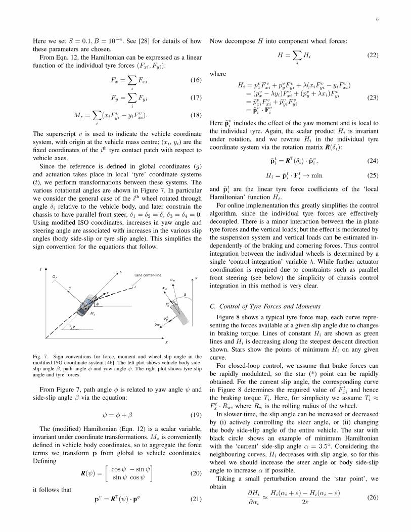
Since the reference is defined in global coordinates (g)and actuation takes place in local ‘tyre’ coordinate systems(t), we perform transformations between these systems. Thevarious rotational angles are shown in Figure 7. In particularwe consider the general case of the ith wheel rotated throughangle δi relative to the vehicle body, and later constrain thechassis to have parallel front steer, δ1 = δ2 = δ, δ3 = δ4 = 0.Using modified ISO coordinates, increases in yaw angle andsteering angle are associated with increases in the various slipangles (body side-slip or tyre slip angle). This simplifies thesign convention for the equations that follow.

O

y

x

β

ϕ

ψ

v

X

Y

Lane center-line

α

x

Fig. 7. Sign conventions for force, moment and wheel slip angle in themodified ISO coordinate system [46]. The left plot shows vehicle body side-slip angle β, path angle φ and yaw angle ψ. The right plot shows tyre slipangle and tyre forces.

From Figure 7, path angle φ is related to yaw angle ψ andside-slip angle β via the equation:

ψ = φ+ β (19)

The (modified) Hamiltonian (Eqn. 12) is a scalar variable,invariant under coordinate transformations. Mz is convenientlydefined in vehicle body coordinates, so to aggregate the forceterms we transform p from global to vehicle coordinates.Defining

R(ψ) =

[cosψ − sinψsinψ cosψ

](20)

it follows thatpv = RT(ψ) · pg (21)

Now decompose H into component wheel forces:

H =∑i

Hi (22)

where

Hi = pvxFvxi + pvyF

vyi + λ(xiF

vyi − yiF vxi)

= (pvx − λyi)F vxi + (pvy + λxi)Fvyi

= pvxiFvxi + pvyiF

vyi

= pvi · Fvi

(23)

Here pvi includes the effect of the yaw moment and is local tothe individual tyre. Again, the scalar product Hi is invariantunder rotation, and we rewrite Hi in the individual tyrecoordinate system via the rotation matrix R(δi):

pti = RT(δi) · pvi . (24)

Hi = pti · Fti → min (25)

and pti are the linear tyre force coefficients of the ‘localHamiltonian’ function Hi.

For online implementation this greatly simplifies the controlalgorithm, since the individual tyre forces are effectivelydecoupled. There is a minor interaction between the in-planetyre forces and the vertical loads; but the effect is moderated bythe suspension system and vertical loads can be estimated in-dependently of the braking and cornering forces. Thus controlintegration between the individual wheels is determined by asingle ‘control integration’ variable λ. While further actuatorcoordination is required due to constraints such as parallelfront steering (see below) the simplicity of chassis controlintegration in this method is very clear.

C. Control of Tyre Forces and Moments

Figure 8 shows a typical tyre force map, each curve repre-senting the forces available at a given slip angle due to changesin braking torque. Lines of constant Hi are shown as greenlines and Hi is decreasing along the steepest descent directionshown. Stars show the points of minimum Hi on any givencurve.

For closed-loop control, we assume that brake forces canbe rapidly modulated, so the star (*) point can be rapidlyobtained. For the current slip angle, the corresponding curvein Figure 8 determines the required value of F txi and hencethe braking torque Ti. Here, for simplicity we assume Ti ≈F tx ·Rw, where Rw is the rolling radius of the wheel.

In slower time, the slip angle can be increased or decreasedby (i) actively controlling the steer angle, or (ii) changingthe body side-slip angle of the entire vehicle. The star withblack circle shows an example of minimum Hamiltonianwith the ‘current’ side-slip angle α = 3.5◦. Considering theneighbouring curves, Hi decreases with slip angle, so for thiswheel we should increase the steer angle or body side-slipangle to increase α if possible.

Taking a small perturbation around the ‘star point’, weobtain

∂Hi

∂αi≈ Hi(αi + ε)−Hi(αi − ε)

2ε(26)

7

! steepest descent direction

4.0°

3.5°

3.0°

Fig. 8. Force map in tyre coordinates: each solid curve represents the rangeof forces available due to changes in braking torque for a given slip angle.Lines of constant Hi are normal to the direction of steepest descent. Starsdenote the points of minimum Hi on each curve.

It is easy to show that when the vehicle side-slip angle βis small,

αi = δi + β − v−1x ψxi (27)

In the following we assume the following actuators: frontaxle steer with δ1 = δ2 = δ and the four independent wheelbraking torques Ti. Coordination of slip angles at the frontaxle takes the form:

Hδ :=∂H

∂δ=∂H1

∂α1· ∂α1

∂δ+∂H2

∂α2· ∂α2

∂δ

=∂H1

∂α1+∂H2

∂α2

(28)

Using Eqn. 26, assuming a steering rate limit kδ for thefront axle steering actuator [23], we locally reduce the valueof H via the control law

δ =

{−kδ sgn(Hδ) |Hδ| > tol0 otherwise (29)

At the rear axle, with no steering actuator available, the bodyside-slip angle is used to modify α3 and α4. This requires yawmoment control and relates back to the desired yaw moment –see Section III-D below. Body side-slip control is determinedin a similar fashion, through the following Equation:

Hβ ≡∂H

∂β=∑i

∂Hi

∂αi· ∂αi∂β

=∑i

∂Hi

∂αi(30)

Similar to Eqn. 29, we define a target side-slip rate basedon the requirement to minimize H

βH =

{−kβ sgn(Hβ), if |Hβ | > tol

0, otherwise(31)

Lateral stability limits are introduced to avoid increasingside-slip angle β beyond some threshold value β2, typically

no more than around 8◦. We introduce a saturation conditionas follows

βd =

−kβ sgn(β), if |β| > β2

0, if |β| > β1⋂ββH > 0

βH , otherwise(32)

where 0 < β1 < β2. While the switching conditions aresomewhat ad-hoc and require separate definition of thresholdparameters (kβ , β1, β2), each parameter has a direct meaningfor controller design and such rules are typical of traditionalcontrol laws for body side-slip [47].

D. Desired Yaw Moment

To complete the MHA algorithm, we need to define thedesired yaw moment Md

z . From Eqn. 19 we determine thedesired yaw rate

ψd = φ+ βd (33)

Variable βd is determined above and φ is related to path curva-ture, which is found from the acceleration in path coordinates

mvφ = mapy = F gy cosφ− F gx sinφ (34)

v being vehicle speed and F g being the force componentsdetermined from the tyre model above. Yaw moments areapplied to track the desired yaw rate via a first order controllaw

τdψ

dt= ψd − ψ (35)

Hence the desired yaw moment is

Mdz = τ−1Izz(ψ

d − ψ) (36)

This completes the definition of the key MHA control equa-tions.

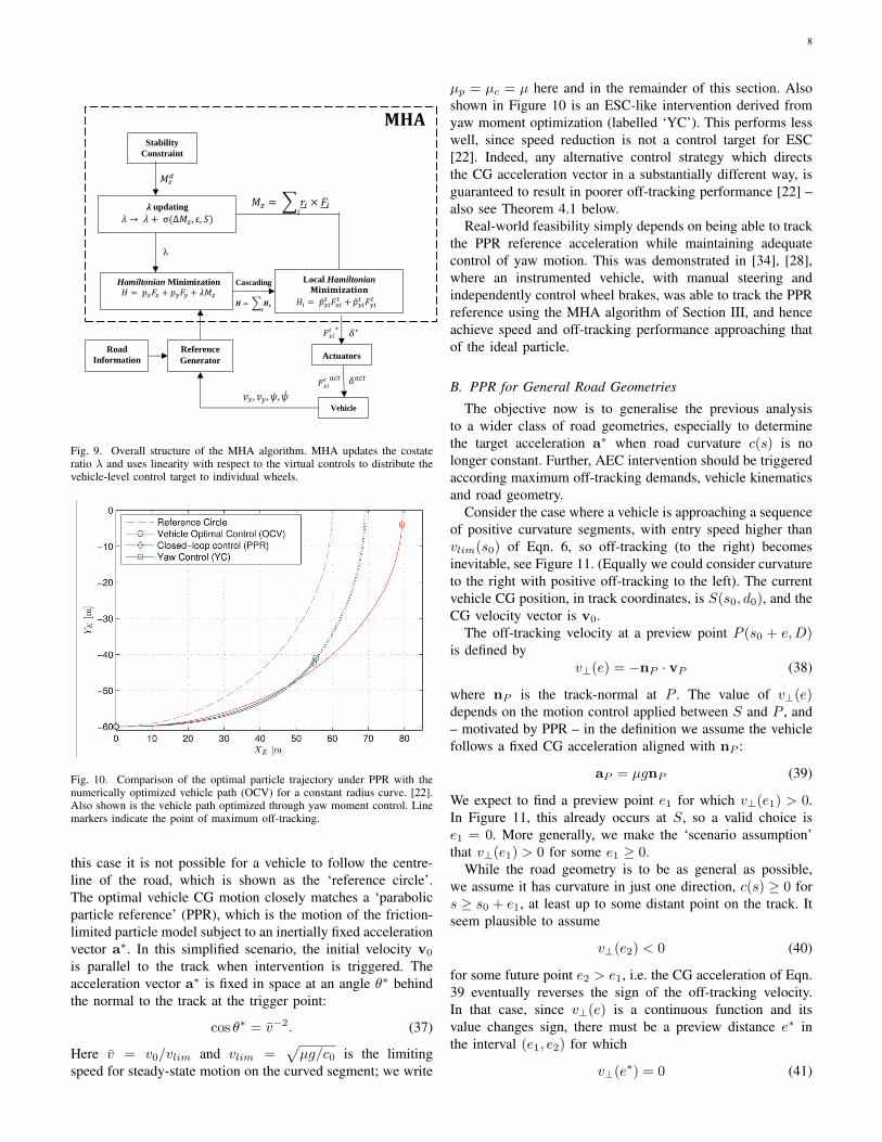
In summary, Figure 9 shows a block diagram of theoverall vehicle-chassis control system. The above equationsdescribes the dashed rectangle block shown as the MHAcontrol allocator. As mentioned previously, MHA performsboth optimization and control allocation. Conventional controlallocation computes the high level virtual controls as targetsfor actuator commands, and solves by further optimization[41], [42], [43]. By contrast, the modified Hamiltonian func-tion is directly resolved into wheel-level components which arethen individually minimized to determine actuator commands.

IV. AEC OPTIMALITY AND REFERENCE ACCELERATION

A. Parabolic Path Reference (PPR)

In earlier work, [22], [34], an optimal control interventionwas determined for an over-speeding vehicle driving on asimple road geometry. There, the road comprised a straightsegment followed by an arc of constant curvature c0. Thecontrol objective was to minimize the maximum radial off-tracking on the curve when the entry speed was higher thanthe limit imposed by friction and curvature – Figure 10. In

8

Reference

Generator

Hamiltonian Minimization

𝐻 = 𝑝𝑥𝐹𝑥 + 𝑝𝑦𝐹𝑦 + 𝜆𝑀𝑧 𝐌𝐢𝐧𝐢𝐦𝐢𝐳𝐚𝐭𝐢𝐨𝐧 Local Hamiltonian

𝐻𝑖 = 𝑝 𝑥𝑖𝑡 𝐹𝑥𝑖

𝑡 + 𝑝 𝑦𝑖𝑡 𝐹𝑦𝑖

𝑡 𝑯 = 𝑯𝒊𝒊

Cascading

Actuators

𝐹𝑥𝑖𝑡 ∗

𝐹𝑥𝑖𝑡 𝑎𝑐𝑡

𝛿∗

𝛿𝑎𝑐𝑡

Vehicle 𝑣𝑥 , 𝑣𝑦 ,𝜓,𝜓

𝜆 → 𝜆 + σ(∆𝑀𝑧 , ε, 𝑆) 𝝀 updating

𝑀𝑧𝑑

Stability

Constraint

λ

𝐌𝐇𝐀

Road

Information

𝑀𝑧 = 𝑟𝑖 × 𝐹𝑖𝑖

Fig. 9. Overall structure of the MHA algorithm. MHA updates the costateratio λ and uses linearity with respect to the virtual controls to distribute thevehicle-level control target to individual wheels.

(OCV) presented above, as well as with the perfor-mance of a closed-loop controller based on YC.

Closed-loop implementation of PPR

It is proposed to use proportional feedback of the dif-ference between the target speed obtained from the par-ticle solution and the actual speed of the vehicle. Bysuitable tuning of the proportional gain, the speed pro-file can be fitted to that of the PPR; then, if the magni-tude of the acceleration of the mass center ismaintained at its limit, the overall acceleration vector isexpected to follow that of the PPR. The target speedfor the particle solution requires knowledge about thetarget curvature kref and the limit speed vlim, which inturn requires an estimate of the surface friction. Sincean intervention is only necessary when v0 . vlim, this sit-uation also implies that the friction limit is reachedsoon after the steering input has been applied. In this

case, mg’

ffiffiffiffiffiffiffiffiffiffiffiffiffiffiffiffiffia2Y + a2X

q, which means that the friction

coefficient can be estimated and thereby vlim is deter-mined from equation (4).

The target speed is vT [ v(T�)= v2lim=v0 according toequation (17). The proportional controller is used todistribute the braking forces to the wheels, and hencethere are four proportional gains, which are denoted gij

and are given by

FXij(t)= � gijmmax (v(t)� vT, 0) ð19Þ

Simple parameter optimization was used to select thegains in equation (19) for best fit to the PPR speed pro-file. The following values were obtained: g11 =0:115,g12 =0:151, g21 =0:081, and g22 =0:114. This implieslarger braking forces at the front wheels, as would beexpected. There is also a bias to increased braking onthe outer wheels, where the vertical load is higher, andso the direct yaw moment from braking acts in theopposite sense to the turn direction; this is contrary tothe standard YC strategy discussed in the first section,suggesting that significant differences will be foundwhen comparing the PPR with YC. This turn-out yawmoment is beneficial for the yaw stability, althoughadditional stabilizing YC would be necessary toaccount for disturbances.

Understeer mitigation by yaw control

We consider a version of the ‘standard’ YC strategy.No attempt is made in this paper to compare with allthe aspects of understeer control of commercial stabi-lity control systems, e.g. engine intervention, but onlyto compare the YC component, a factor that is mostcommonly referenced in the literature. The reason is tomake the comparison clearer; for a comparison with anactual electronic stability control system, we refer toexperimental work reported by Gordon et al.11 Thestandard understeer mitigation proposed in the litera-ture is to apply a turn-in yaw moment by braking the

inner rear wheel. However, care must be taken not toover-brake the single wheel since this can lead to exces-sive sideslip.5 Initial simulations determined that brak-ing both inner wheels was more effective than brakingonly the inner rear wheel (which was also proposed byAntonov7), and so this modification is implemented toimprove the comparative performance of YC. Thus fora left turn ( _c . 0) the longitudinal force vector is

FX11 FX12 FX21 FX22½ �T

= � KP0( _cref � _c) h0 0 (1� h0) 0½ �Tð20Þ

where, based on a neutral steered reference vehicle,

_cref = vXkref ð21Þ

Here KP0 . 0 and 04h041 are tuning parameters,which are optimized in the same way as the gij valueswere optimized for the PPR. The resulting parametervalues are KP0 =18 and h0 =0:7, giving a controllerwith a similar performance to that presented byAntonov.7

Controller evaluation

The results for the two control strategies outlinedabove, together with the open-loop OCV intervention,are shown in Figures 5 to 7. Again we consider the casewith v0 =20 m/s, k�1ref =60 m, and m = 0.4. Closed-loop PPR control is seen to give a close match to OCVin both the path profile and the speed profile (seeFigure 5 and Figure 6(a) respectively). The PPR isshown throughout by open diamonds, while OCV isshown by open circles. Figure 6(c) and (d) shows thatthe closed-loop controller does indeed follow the PPRfor the acceleration of the mass center, approximatingan inertially fixed-mass-center acceleration operating atthe friction limit and with the desired global direction.

Figure 5. Trajectories in global (XE, YE) coordinates: optimizedtwo-track vehicle (OCV), closed-loop PPR strategy and YC.OCV: optimal control for the vehicle; PPR: parabolic path reference; YC:

yaw control.

418 Proc IMechE Part D: J Automobile Engineering 228(4)

Fig. 10. Comparison of the optimal particle trajectory under PPR with thenumerically optimized vehicle path (OCV) for a constant radius curve. [22].Also shown is the vehicle path optimized through yaw moment control. Linemarkers indicate the point of maximum off-tracking.

this case it is not possible for a vehicle to follow the centre-line of the road, which is shown as the ‘reference circle’.The optimal vehicle CG motion closely matches a ‘parabolicparticle reference’ (PPR), which is the motion of the friction-limited particle model subject to an inertially fixed accelerationvector a∗. In this simplified scenario, the initial velocity v0

is parallel to the track when intervention is triggered. Theacceleration vector a∗ is fixed in space at an angle θ∗ behindthe normal to the track at the trigger point:

cos θ∗ = v−2. (37)

Here v = v0/vlim and vlim =õg/c0 is the limiting

speed for steady-state motion on the curved segment; we write

µp = µc = µ here and in the remainder of this section. Alsoshown in Figure 10 is an ESC-like intervention derived fromyaw moment optimization (labelled ‘YC’). This performs lesswell, since speed reduction is not a control target for ESC[22]. Indeed, any alternative control strategy which directsthe CG acceleration vector in a substantially different way, isguaranteed to result in poorer off-tracking performance [22] –also see Theorem 4.1 below.

Real-world feasibility simply depends on being able to trackthe PPR reference acceleration while maintaining adequatecontrol of yaw motion. This was demonstrated in [34], [28],where an instrumented vehicle, with manual steering andindependently control wheel brakes, was able to track the PPRreference using the MHA algorithm of Section III, and henceachieve speed and off-tracking performance approaching thatof the ideal particle.

B. PPR for General Road Geometries

The objective now is to generalise the previous analysisto a wider class of road geometries, especially to determinethe target acceleration a∗ when road curvature c(s) is nolonger constant. Further, AEC intervention should be triggeredaccording maximum off-tracking demands, vehicle kinematicsand road geometry.

Consider the case where a vehicle is approaching a sequenceof positive curvature segments, with entry speed higher thanvlim(s0) of Eqn. 6, so off-tracking (to the right) becomesinevitable, see Figure 11. (Equally we could consider curvatureto the right with positive off-tracking to the left). The currentvehicle CG position, in track coordinates, is S(s0, d0), and theCG velocity vector is v0.

The off-tracking velocity at a preview point P (s0 + e,D)is defined by

v⊥(e) = −nP · vP (38)

where nP is the track-normal at P . The value of v⊥(e)depends on the motion control applied between S and P , and– motivated by PPR – in the definition we assume the vehiclefollows a fixed CG acceleration aligned with nP :

aP = µgnP (39)

We expect to find a preview point e1 for which v⊥(e1) > 0.In Figure 11, this already occurs at S, so a valid choice ise1 = 0. More generally, we make the ‘scenario assumption’that v⊥(e1) > 0 for some e1 ≥ 0.

While the road geometry is to be as general as possible,we assume it has curvature in just one direction, c(s) ≥ 0 fors ≥ s0 + e1, at least up to some distant point on the track. Itseem plausible to assume

v⊥(e2) < 0 (40)

for some future point e2 > e1, i.e. the CG acceleration of Eqn.39 eventually reverses the sign of the off-tracking velocity.In that case, since v⊥(e) is a continuous function and itsvalue changes sign, there must be a preview distance e∗ inthe interval (e1, e2) for which

v⊥(e∗) = 0 (41)

9

Pe

Pn

)0,( 0sS

)0,( 0 esP

PpP g na

),( 0 dsSPv

0v

),( 0 DesP

P

Q

0v

PvP

S

Pn

h

L

P

H

Fig. 11. Geometric definition of the previewed lateral velocity v⊥. Parabolicmotion occurs under constant acceleration aP . Unit vectors eP , nP respec-tively define the track tangent and normal at the previewed point P ′ on thetrack centre-line (dashed curve). h is the distance between S and the tracknormal, with SH drawn parallel to eP . v⊥ is the component of vP in thedirection −nP . Line SQ represents an alternative motion under straight-linebraking, and L = |SQ| is the minimum stopping distance.

If more than one such point exists, the value of e2 can bereduced so that e∗ is a unique solution.

The existence of e2, and hence e∗ may seem obvious: aconcerted path-lateral control effort will eventually reverse theoff-tracking tendency. However, it seems important enough toprovide a formal verification – Appendix A. Here the generalreasoning is given. Referring to Figure 11, motion parallelto eP is orthogonal to the acceleration vector and hence thevelocity component is constant. Hence the time to reach Pfrom S is found from distance h:

TP =h

v0 cos θ(42)

Motion parallel to nP has constant acceleration µg and hence

v⊥ = v0 sin θ − µgTP

= v0 sin θ − µgh

v0 cos θ(43)

Introducing the minimum straight-line stopping distance L,then v20 = 2µgL , and Eqn. 43 for the lateral velocity is re-written:

v⊥ =v0

2 cos θ·(

sin 2θ − h

L

). (44)

Hence, increasing the preview distance will typically cause hin Figure 11 to exceed L, so the bracketed expression in Eqn.44 becomes negative, showing that both e2 and e∗ exist.

Writing P ∗ for the vertex of the parabola associated with e∗

we propose the following inertially-fixed acceleration vectoras the required PPR generalization:

a∗ = µgn∗ (45)

where n∗ = nP∗ is the track normal at P ′∗.

C. PPR Optimality

In [22], PPR optimality for the constant radius curve wasderived using Pontryagin’s Minimum Principle. Here, an al-ternative geometric analysis is provided.

Theorem 4.1 (PPR Optimality): Under the scenario assump-tions above, control from S under constant acceleration a∗

is optimal for the friction-limited particle, i.e. for any othercontrol strategy, maximum off-tracking is greater than formotion under a∗.

Proof Introduce local coordinates (ξ, η), as shown in Figure12, with origin at S and axes aligned with the track normaland tangent unit vectors at P ′∗. The candidate optimal controlresults in a path (ξ1(t), η1(t)) from S to P ∗, which is thevertex of the parabola. Since c(s) ≥ 0, it is sufficient toshow that any other feasible control input has a trajectory(ξ2(t), η2(t)) that penetrates the shaded region in the figure,for in that case off-tracking clearly exceeds distance |P ∗P ′∗|.

0v

a

0v

*a

*P *P

*PS

*P

*

Fig. 12. Coordinates (ξ, η) aligned to the track normal n∗ and tangent e∗at P ′∗. The optimizing acceleration vector a∗ is parallel to n∗. P ∗ is thevertex of the optimizing parabola.

The candidate optimal trajectory satisfies the equations

ξ1 = −µg , η1 = 0 (46)

with initial conditions (see Figure 12) ξ1(0) = 0, ξ1(0) =v0 sin θ∗, η1(0) = 0, η1(0) = v0 cos θ∗. We set t = 0 at pointS, and write t = T ∗ at the vertex.

From the friction constraint, Eqn. 4, any alternative trajec-tory ξ2(t) satisfies an equation of the form:

ξ2 = −µg + α(t) (47)

where α(t) ≥ 0 and α(t) > 0 for some finite period of time –otherwise, from the constraint, η2 = 0 and the same parabolictrajectory is followed.

The deviation in ξ between the two trajectories is ξe =(ξ2 − ξ1). Then

ξe = α(t) ≥ 0 (48)

with zero initial conditions. Integrating twice with respect tot:

ξe(T∗) =

∫ T∗

0

∫ t′

0

α(t) dt dt′ > 0 (49)

10

Hence, at time T ∗, ξ2 > ξP∗ and the alternative trajectorypenetrates the shaded region. Hence off-tracking is greater thanfor the candidate optimal control.

Apex point. In Figure 12, P ∗ determines where maximumoff-tracking will occur, assuming an ideal control intervention.The off-tracking distance D∗ = |P ∗P ′∗| gives a best-caseestimate of the maximum future off-tracking. This is valid anduseful even if the AEC chassis controller cannot perfectlymatch the acceleration reference. The above theorem showsthat maximum off-tracking is entirely dependent on the CGacceleration response in comparison to the reference particle.The vertex of the optimizing parabola, P ∗, will be calledthe ‘apex point’. Finding P ∗ is crucial for the AEC triggerand control reference, and is found by searching an on-boarddigital map – see below.

The above generalizes the PPR analysis of [22], where inFigure 11 the track ahead of s0 has constant curvature c0 =R−10 and intervention is triggered with S on the track centre-line (i.e. d = 0); further, v0 is parallel to the track tangent.Simple geometry gives h = R0 sin θ, and from Eqn. 43, v⊥=0occurs when

v0 sin θ =µgR0 sin θ

v0 cos θ(50)

and hence the optimizing angle is given by

v20 cos θ∗ = µg/c0 (51)

in agreement with Eqn. 37.

D. AEC Trigger and Apex Search

As discussed, AEC is to trigger when the best-case predictedoff-tracking exceeds some prescribed threshold, D∗ > D0.In the following, an implementable algorithm is proposed forfinding and evaluating the apex point P ∗, and hence decidingif and when to trigger AEC.

First, an AEC event flag fe is introduced, to represent thefollowing conditions:

fe =

+1, AEC function on, left turn−1, AEC function on, right turn0, AEC function off.

(52)

During normal driving, fe = 0, and this ‘off-state’ is main-tained until v ≥ vlim is detected. In that case a functionFaec(Γ, fe) is evaluated

Faec : (Γ, fe) 7→ (P ∗,a∗, f ′e) (53)

where f ′e is the updated event flag and Γ denotes the geometricand kinematic information required at each time step by theAEC function. Γ consists of the position and velocity statesof the vehicle, together with a digital map giving the roadinformation (geometry and friction level). If P ∗ is foundwith D∗ > D0, then f ′e = ±1 is returned, together withthe acceleration reference a∗. During the following, Faec isevaluated at each time-step to give an updated a∗. Finally,the AEC intervention finishes when the local lateral velocityv⊥(0) switches from positive to negative. The overall decisionlogic is given in Figure 13.

v ≥ vlim

Apply Faec

Type equation here.

𝐷∗ ≥ 𝐷0?

True

True

True

𝑓𝑒 = ±1

Nex

t t

Start t = 0

𝑓𝑒 = 0 ?

True

Apply Faec False

v⊥(0) < 0?

𝑓𝑒 = 0 True

False

False

False

Update 𝒂∗

Fig. 13. Flow chart of the AEC reference / trigger system. Control is onlyapplied when fe = ±1, which requires the initial detection of an over-speedcondition as well as continuous reporting of a valid detection. Interventioncontinues with updating of a∗ (closed loop) until v0⊥ < 0 indicates the endof the intervention.

Function Faec determines the initial choice of dominantroad curvature using the position of point Q in Figure 11,as determined from v0 and the straight-line braking distance.If the lateral coordinate is negative, sy(Q) < 0, the overallcurvature is deemed positive. In general,

fe = − sgn(sy(Q)). (54)

Next, Faec performs a one-dimensional numerical search forthe apex point, starting at the preview distance of Q,

e0 = sx(Q)− s0 (55)

If v⊥(e0) > 0 the search is carried out forwards, with e > e0;if v⊥(e0) < 0 the search is backwards, with e < e0. In eithercase, the apex point is found with v⊥(e∗) = 0 and hence P ∗

and a∗ are determined.

V. RESULTS

A. Hockenheim circuit

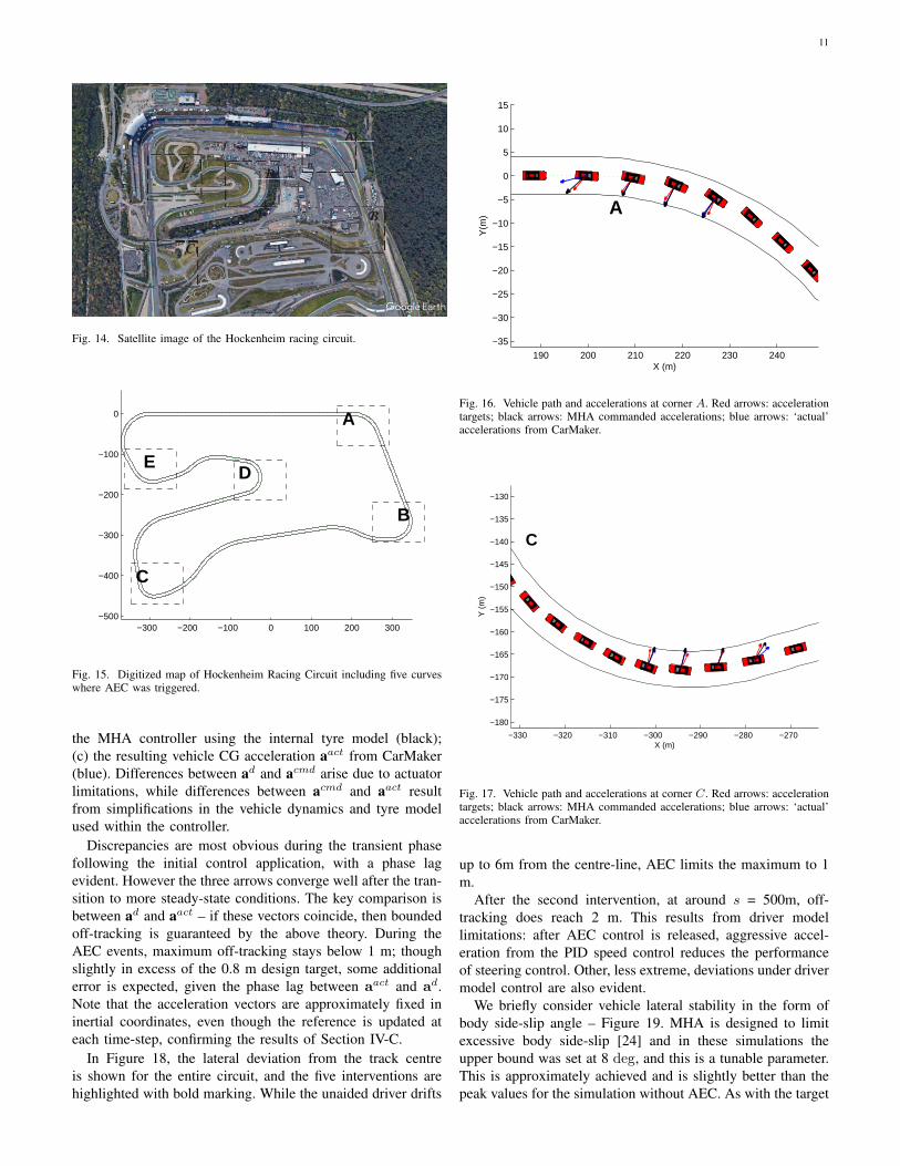
Here the AEC system is tested in simulation, using therelatively complex geometry of the Hockenheim racing circuit.Figure 14 shows a satellite image and Figure 15 highlights anumber of curves of interest. As mentioned in Section II-E,ROR risk was artificially created by including a time delayin the speed controller, so that braking into curves is delayed.Setting D0 = 0.8 m in the above algorithm, vehicle simulationwas performed using CarMaker, both with and without AECprotection.

AEC was triggered on the five curves, labelled A to E,and Figures 16, 17 show the vehicle path and CG accel-eration on two of these curves. Three acceleration vectorsare shown in each plot, also indicating the times when AECis active. These are: (a) the desired acceleration referencead = a∗ obtained from Faec (red); (b) acmd predicted from

11

A

B

C

D E

Fig. 14. Satellite image of the Hockenheim racing circuit.

−300 −200 −100 0 100 200 300−500

−400

−300

−200

−100

0

E

B

C

D

A

Fig. 15. Digitized map of Hockenheim Racing Circuit including five curveswhere AEC was triggered.

the MHA controller using the internal tyre model (black);(c) the resulting vehicle CG acceleration aact from CarMaker(blue). Differences between ad and acmd arise due to actuatorlimitations, while differences between acmd and aact resultfrom simplifications in the vehicle dynamics and tyre modelused within the controller.

Discrepancies are most obvious during the transient phasefollowing the initial control application, with a phase lagevident. However the three arrows converge well after the tran-sition to more steady-state conditions. The key comparison isbetween ad and aact – if these vectors coincide, then boundedoff-tracking is guaranteed by the above theory. During theAEC events, maximum off-tracking stays below 1 m; thoughslightly in excess of the 0.8 m design target, some additionalerror is expected, given the phase lag between aact and ad.Note that the acceleration vectors are approximately fixed ininertial coordinates, even though the reference is updated ateach time-step, confirming the results of Section IV-C.

In Figure 18, the lateral deviation from the track centreis shown for the entire circuit, and the five interventions arehighlighted with bold marking. While the unaided driver drifts

190 200 210 220 230 240

−35

−30

−25

−20

−15

−10

−5

0

5

10

15

X (m)

Y(m

) A

Fig. 16. Vehicle path and accelerations at corner A. Red arrows: accelerationtargets; black arrows: MHA commanded accelerations; blue arrows: ‘actual’accelerations from CarMaker.

−330 −320 −310 −300 −290 −280 −270

−180

−175

−170

−165

−160

−155

−150

−145

−140

−135

−130

X (m)

Y (

m)

C

Fig. 17. Vehicle path and accelerations at corner C. Red arrows: accelerationtargets; black arrows: MHA commanded accelerations; blue arrows: ‘actual’accelerations from CarMaker.

up to 6m from the centre-line, AEC limits the maximum to 1m.

After the second intervention, at around s = 500m, off-tracking does reach 2 m. This results from driver modellimitations: after AEC control is released, aggressive accel-eration from the PID speed control reduces the performanceof steering control. Other, less extreme, deviations under drivermodel control are also evident.

We briefly consider vehicle lateral stability in the form ofbody side-slip angle – Figure 19. MHA is designed to limitexcessive body side-slip [24] and in these simulations theupper bound was set at 8 deg, and this is a tunable parameter.This is approximately achieved and is slightly better than thepeak values for the simulation without AEC. As with the target

12

bound for off-tracking, there is some additional deviation dueto transients, but overall lateral stability is maintained. Tightercontrol of body side-slip is possible, but if the upper bound istoo small it will restrict the lateral forces at the rear axle andhence reduce acceleration tracking performance.

0 500 1000 1500 2000 2500

Sx (m)

-2

-1.5

-1

-0.5

0

0.5

1

1.5

2

Sy (

m)

0 500 1000 1500 2000 2500

Vehicle route / path coordinate (m)

-6

-4

-2

0

2

4

6

s y (m

)

driver controlAEC

AEC on

Fig. 18. Vehicle path plots in track coordinates. Bold markers indicatestimes when AEC is active.

0 20 40 60 80 100 120

time (sec)

-10

-5

0

5

10

15

20

body

sid

eslip

ang

le (

deg)

driver modelAEC

Fig. 19. Vehicle body side-slip angle. Bold line style indicates systeminterventions.

Figure 20 shows the front axle steering angle, with reddots highlighting the five interventions. Figure 21 shows thedirect yaw moment contribution from the brake actuators (red),which provides roughly 50% of the total yaw moment (shownin black). Some brake torque ‘chatter’ is seen towards the endof some of the events.

B. Highway Entry Curve with Reduced Friction

Here the scenario is a highway entry road with low sur-face friction (µs = 0.4) shown in Figure 22. The vehicleapproaches from the right and eventually merges onto thehighway. To represent the case where the driver over-estimatesthe road friction, vlim used by the driver model is set with µp =0.42 while AEC is presumed aware of the lower friction withµs = 0.4 in the tyre model. Further, a conservative particlefriction µc = 0.35 is used within the AEC algorithm. Thevehicle path is shown Figure 23. With AEC enabled, maximumoff-tracking is limited to around 1.5m. The acceleration vectorsshow slightly greater overall dispersion than previously, ex-plaining the slightly greater off-tracking. It can be seen that theuncontrolled vehicle leaves the road (and the simulation stops).Note that the vehicle acceleration vector (blue arrow) hasreduced magnitude compared with the expected acceleration(black arrow) and again there are transient delays apparent.There are seen to be three sub-interventions on the singlecurve, due to the tightening curvature and the driver modelincreasing speed whenever AEC is switched off.

0 10 20 30 40 50 60 70 80 90 100

Time (sec)

-10

-8

-6

-4

-2

0

2

4

6

8

/ (

deg)

Fig. 20. Steering inputs at the front axle. AEC-controlled steering inputsare shown as red dots.

6.2 6.4 6.6 6.8 7 7.2 7.4 7.6 7.8-8000

-6000

-4000

-2000

0

2000

Mz

at A

(N

m)

17.8 18 18.2 18.4 18.6 18.8 19 19.2 19.4 19.6-8000

-6000

-4000

-2000

0

2000

Mz

at B

(N

m)

45.5 46 46.5 47 47.5 48 48.5 49-8000

-6000

-4000

-2000

0

2000

Mz

at C

(N

m)

66 66.5 67 67.5 68 68.5 69

Time (sec)

-2000

0

2000

4000

6000

Mz

at D

(N

m)

Mz from braking forcestotal Mz

Fig. 21. Yaw moments due to MHA action at curves A to D. The direct yawmoment from braking is shown in red dashed line, comprising roughly 50% of thetotal, shown in black.

Fig. 22. Highway entry curve Rasserodsmotet, Uddevalla, Sweden; mapof selected road geometry with fitted track model (courtesy: Google Maps,lat.58.3506, long.11.9797)

Here the various control system parameters were left un-changed from the previous scenario, i.e. there was no re-tuningof the MHA parameters other than to revise the friction esti-mates. The MHA internal tyre model was re-scaled accordingto the new value of µs, and no further tyre model fitting wascarried out. Example tyre forces are shown in Figure 24, herefor the first AEC intervention. At the front-left wheel, F tx

13

−160 −140 −120 −100 −80 −60 −40

Fig. 23. Vehicle path on a highway entry curve; blue vehicle - no AEC systemintervention; red vehicle - AEC system eneabled. Arrow labels: see Figure 16caption.

follows the control input slightly better than for F ty , whilefor the rear-right tyre both force components are tracked well.

10 10.5 11 11.5 12 12.5 13 13.5 14

time(sec)

-1500

-1000

-500

0

500

Fxfl (

N)

10 10.5 11 11.5 12 12.5 13 13.5 14

time(sec)

-2000

-1500

-1000

-500

0

Fyfl (

N)

Fig. 24. Longitudinal and lateral tyre force control at the front-left tyre onthe highway entry curve. The blue solid lines represents the ‘actual’ tyreforces (CarMaker output). The red dotted lines are the commanded forcesfrom MHA.

VI. CONCLUSION

This paper has presented theory, algorithms and simulationsto formulate and test a concept for a future Automated Emer-gency Cornering (AEC) system. The proposed AEC systemuses a digital map and vehicle kinematic data to trigger andupdate the motion reference. It also requires friction estima-tion to perform in a near-optimal way. It has a hierarchicalstructure, the upper level based on an optimal particle model,the lower level distributing control objectives via the MHAmethod. MHA has been shown capable of real-time operationand is equally applicable to high and low friction surfaces.

10 10.5 11 11.5 12 12.5 13 13.5 14-800

-600

-400

-200

0

Fxrr

(N

)

10 10.5 11 11.5 12 12.5 13 13.5 14

time (sec)

-800

-600

-400

-200

0

Fxrr

(N

)

Fig. 25. Longitudinal and lateral tyre force control at the rear-right tyre (asfor Figure 24).

In simulation, the proposed AEC system successfully pre-vented road departures, analogous to the way AutonomousEmergency Braking (AEB) systems anticipate and mitigatefrontal collisions. AEC intervention was triggered at the pointwhen further delay or sub-optimal response will necessarilylead to excessive lane departure. Because the system usesall available actuators and all available friction, a humandriver could not be expected to achieve similar off-trackingperformance, except by intervening earlier. Hence AEC is notexpected to interfere with normal driving.

While simplified models are used for theoretical develop-ment and within in the controller, the high-fidelity vehicledynamics software CarMaker was used to test the ability ofAEC to achieve its purpose. The AEC system compares wellto the predictions from the friction-limited particle on the highfriction tests. On the lower friction there are longer transientdelays is building the required forces, and some compensationmay be necessary in terms of trigger timing. While refinementswill be needed for robust implementation, this paper hasdefined the essential building blocks of a feasible AEC system.

APPENDIX ALATERAL VELOCITY REVERSAL

This appendix verifies the existence of e2 for the particlemotion under constant acceleration aP given in Eqn. 39,assuming the conditions of Section IV-C:

1) e1 > 0 exists such that v⊥(e1) > 0 (scenario assumption)2) v0 > vlim(s0) (over-speed condition)3) c(e) ≥ 0 for e ≥ e1 (unidirectional curvature)

The scenario of Figure 11 is drawn again in Figure 26, nowwith initial point S corresponding to e = e1 and thereforev⊥(S) > 0. Inertial coordinates (X,Y ) are selected at thispoint, with the X-axis parallel to the track tangent. The dashedcurve SP ′ follows the path of the track but may be laterallyoffset at a constant distance from the track centre-line. Hereu denotes the longitudinal distance from S along the curve;because of lateral offset, it differs slightly from the centre-linedistance e− e1, but is more convenient for this analysis.

14

𝑆 𝑋

𝑌

𝜃1

ℎ

𝜃0

P

P

H

P

u

Fig. 26. Particle motion from S to P along a path of positive curvature.θ = θ0 + θ1 is the angle given in Eqn. 56.

For preview point P , the track-normal is drawn to definepoints P ′, P ′′, as shown; line SH is parallel to the tracktangent and is hence normal to line PH . Angle θ = θ0 + θ1is the angle between the current path and the normal at thepreview point. Condition c(e) ≥ 0 implies θ1 is a non-decreasing function of u, while v⊥(S) > 0 implies θ0 > 0.

The requirement is to show v⊥(e) < 0 for some e > e1.Equivalently, the bracketed expression in Eqn. 44 shouldbecome negative for some u > 0:

sin 2θ − h

L< 0 (56)

Since the stopping distance L is a positive constant, andh ≥ 0 for all possible road geometries, Eqn. 56 is immediatelysatisfied if sin 2θ < 0, i.e. if θ > π/2 for a sufficiently largedistance along the track.

Hence we can limit attention to the case where the roaddoes not turn through a full 90◦ within the assumed previewhorizon. Then we naturally expect h to increase without anyupper limit and this is now shown.

θ1 ≤ π/2− θ0. (57)

and hence cos θ1 is bounded below

cos θ1 ≥ sin θ0 > 0 (58)

In Figure 26, let x be the X-coordinate of point P ′. Sincethe tangent at P ′ is parallel to line SH ,

dx

dy= cos θ1 (59)

Hence, using Eqn. 58,

x(u) =

∫cos θ1 du ≥

∫sin θ0 du = u sin θ0 (60)

Also, it is clear that distance |SP ′′| = h/ cos θ1 is greaterthan x, hence

h ≥ x cos θ1 ≥ x sin θ0 ≥ u sin2 θ0. (61)

where Eqn. 60 has been used. Hence, if u > L/ sin2 θ0, Eqn.56 is again satisfied.

APPENDIX BVEHICLE PARAMETERS

Parameter PhysicalMeaning

Unit Value

m total mass kg 1174ms sprung mass kg 1020mu unsprung mass kg 154Izz yaw moment of

inertiakgm2 1360

Ixx roll moment ofinertia

kgm2 350

Iyy pitch moment ofinertia

kgm2 1290

lf CG to front axle m 1.043lr CG to rear axle m 1.637w track width m 1.530h mass centre hight m 0.605µp particle friction

coefficient- 0.8

µc AEC-estimatedfriction

- 0.8

µs surface frictionof the tyre model

- 1.0

Rw loaded tyre ra-dius

m 0.3

Iw nominal wheelrotational inertia

kgm2 0.5

Λ front and rearsuspension ratio

- 0.5

ρ air mass density kgm3 1.2Cd air drag coeffi-

cient- 0.3

AF front area of thevehicle

m2 2.4

τ brake/drivetorque timeconstant

s 0.05

B,C,D,E MF tyre coeffi-cients

- 0.7094,1.4097,1.0,0

iS steering systemratio

- 17.0

REFERENCES

[1] Lotta Jakobsson, Magdalena Lindman, Anders Axelson, Bengt Lokens-gard, Mats Petersson, Bo Svanberg, and Jordanka Kovaceva. Addressingrun off road safety. SAE International Journal of Passenger Cars-Mechanical Systems, 7(2014-01-0554):132–144, 2014.

[2] Cejun Liu and Rajesh Subramanian. Factors related to fatal single-vehicle run-off-road crashes. Technical report, 2009.

[3] Cejun Liu and Tony Jianqiang Ye. Run-off-road crashes: an on-sceneperspective. Technical report, 2011.

[4] David LeBlanc. Road departure crash warning system field operationaltest: methodology and results. volume 1: technical report. 2006.

[5] John Vincent Bond III, Gerald H Engelman, Jonas Ekmark, Jonas LZJansson, M Nabeel Tarabishy, and Levasseur Tellis. Autonomousemergency braking system, February 25 2003. US Patent 6,523,912.

[6] Jessica B Cicchino. Effectiveness of forward collision warning systemswith and without autonomous emergency braking in reducing police-reported crash rates. Arlington, VA: Insurance Institute for HighwaySafety, 2016.

[7] David J LeBlanc, Gregory E Johnson, Paul J Th Venhovens, GarthGerber, Robert DeSonia, Robert D Ervin, Chiu-Feng Lin, A Galip Ulsoy,and Thomas E Pilutti. Capc: A road-departure prevention system. IEEEControl Systems Magazine, 16(6):61–71, 1996.

[8] Vassilios Morellas, Ted Morris, Lee Alexander, and Max Donath.Preview based control of a tractor trailer using dgps for preventingroad departure accidents. In Proceedings of Conference on IntelligentTransportation Systems, pages 797–805. IEEE, 1997.

[9] Parag H Batavia, Dean A Pomerleau, and Charles E Thorpe. Predictinglane position for roadway departure prevention. In Proceedings of theIEEE intelligent vehicles symposium, pages 245–251, 1998.

[10] Claudio Rosito Jung and Christian Roberto Kelber. Lane followingand lane departure using a linear-parabolic model. Image and VisionComputing, 23(13):1192–1202, 2005.

15

[11] A Kullack, I Ehrenpfordt, K Lemmer, and F Eggert. Reflektas:lane departure prevention system based on behavioural control. IETIntelligent Transport Systems, 2(4):285–293, 2008.

[12] Yasuhisa Hayakawa, Kou Sato, Yoshiaki Tabata, and Kenichi Egawa.Design of a lane departure prevention system with enhanced drivabil-ity. SAE International Journal of Passenger Cars-Mechanical Systems,2(2009-01-0160):398–403, 2009.

[13] Nicoleta Minoiu Enache, Said Mammar, Sebastien Glaser, and BenoitLusetti. Driver assistance system for lane departure avoidance bysteering and differential braking. IFAC Proceedings Volumes, 43(7):471–476, 2010.

[14] D Katzourakis, Mohsen Alirezaei, Joost CF de Winter, Matteo Corno,Riender Happee, A Ghaffari, and R Kazemi. Shared control forroad departure prevention. In 2011 IEEE International Conference onSystems, Man, and Cybernetics, pages 1037–1043. IEEE, 2011.

[15] Abdelkader Merah, Kada Hartani, and Azeddine Draou. A new sharedcontrol for lane keeping and road departure prevention. Vehicle SystemDynamics, 54(1):86–101, 2016.

[16] Dongkui Tan, Wuwei Chen, Hongbo Wang, and Zhengang Gao. Sharedcontrol for lane departure prevention based on the safe envelope ofsteering wheel angle. Control Engineering Practice, 64:15–26, 2017.

[17] Yiannis E Papelis, Ginger S Watson, and Timothy L Brown. Anempirical study of the effectiveness of electronic stability control systemin reducing loss of vehicle control. Accident Analysis & Prevention,42(3):929–934, 2010.

[18] Sehyun Chang and Timothy J Gordon. Model-based predictive control ofvehicle dynamics. International Journal of Vehicle Autonomous Systems,5(1-2):3–27, 2007.

[19] Paolo Falcone, Francesco Borrelli, H Eric Tseng, Jahan Asgari, andDavor Hrovat. A hierarchical model predictive control framework forautonomous ground vehicles. In American Control Conference, 2008,pages 3719–3724. IEEE, 2008.

[20] Javad Ahmadi, Ali Khaki Sedigh, and Mansour Kabganian. Adaptivevehicle lateral-plane motion control using optimal tire friction forceswith saturation limits consideration. IEEE Transactions on vehiculartechnology, 58(8):4098–4107, 2009.

[21] Derong Yang, Timothy J Gordon, Bengt Jacobson, and Mats Jonasson.Quasi-linear optimal path controller applied to post impact vehicledynamics. IEEE transactions on intelligent transportation systems,13(4):1586–1598, 2012.

[22] Matthijs Klomp, Mathias Lidberg, and Timothy J Gordon. On optimalrecovery from terminal understeer. Proceedings of the Institution ofMechanical Engineers, Part D: Journal of Automobile Engineering,228(4):412–425, 2014.

[23] Derong Yang, Bengt Jacobson, Mats Jonasson, and Tim J Gordon.Closed-loop controller for post-impact vehicle dynamics using individualwheel braking and front axle steering. International Journal of VehicleAutonomous Systems, 12(2):158–179, 2014.

[24] Yangyan Gao, Mathias Lidberg, and Timothy Gordon. Modified hamil-tonian algorithm for optimal lane change with application to collisionavoidance. MM Science Journal MAR, pages 576–584, 2015.

[25] John K Subosits and J Christian Gerdes. A synthetic input approachto slip angle based steering control for autonomous vehicles. In 2017American Control Conference (ACC), pages 2297–2302. IEEE, 2017.

[26] Hongyan Guo, Feng Liu, Fang Xu, Hong Chen, Dongpu Cao, and YanJi. Nonlinear model predictive lateral stability control of active chassisfor intelligent vehicles and its fpga implementation. IEEE Transactionson Systems, Man, and Cybernetics: Systems, 2017.

[27] Vincent A Laurense, Jonathan Y Goh, and J Christian Gerdes. Path-tracking for autonomous vehicles at the limit of friction. In 2017American Control Conference (ACC), pages 5586–5591. IEEE, 2017.

[28] Y Gao. Vehicle Motion and Stability Control at the Limits of Handlingvia the Modified Hamiltonian Algorithm. PhD thesis, University ofLincoln, 2018.

[29] Mohammadhossein Malmir, Marco Baur, and Luca Bascetta. A modelpredictive controller for minimum time cornering. In 2018 InternationalConference of Electrical and Electronic Technologies for Automotive,pages 1–6. IEEE, 2018.

[30] Victor Fors, Bjorn Olofsson, and Lars Nielsen. Slip-angle feedbackcontrol for autonomous safety-critical maneuvers at-the-limit of friction.In International Symposium on Advanced Vehicle Control (AVEC), 2018.

[31] Joseph Funke, Matthew Brown, Stephen M Erlien, and J ChristianGerdes. Collision avoidance and stabilization for autonomous vehiclesin emergency scenarios. IEEE Transactions on Control Systems Tech-nology, 25(4):1204–1216, 2017.

[32] Andras Mihaly, Balazs Nemeth, and Peter Gaspar. Look-ahead controlof road vehicles for safety and economy purposes. In 2014 EuropeanControl Conference (ECC), pages 714–719. IEEE, 2014.

[33] Yangyan Gao, Timothy Gordon, and Mathias Lidberg. A flexible controlallocation method for terminal understeer mitigation. In Students onApplied Engineering (ICSAE), International Conference for, pages 18–23. IEEE, 2016.

[34] Yangyan Gao, Timothy Gordon, and Mathias Lidberg. Implementationof a modified hamiltonian algorithm for control allocation. In AdvancedVehicle Control: Proceedings of the 13th International Symposium onAdvanced Vehicle Control (AVEC’16), September 13-16, 2016, Munich,Germany, page 157. CRC Press, 2016.

[35] IPG CarMaker. Users guide version 4.5. 2. IPG Automotive, Karlsruhe,Germany, 2014.

[36] Hans B Pacejka and Egbert Bakker. The magic formula tyre model.Vehicle system dynamics, 21(S1):1–18, 1992.

[37] William F Milliken, Douglas L Milliken, et al. Race car vehicledynamics, volume 400. Society of Automotive Engineers Warrendale,1995.

[38] Hans B Pacejka. Tyre and vehicle dynamics, p 511-562. Delft Universityof Technology, 2002.

[39] TJ Gordon and Matt C Best. On the synthesis of driver inputs for thesimulation of closed-loop handling manoeuvres. International Journalof Vehicle Design, 40(1-3):52–76, 2005.

[40] IPG CarMaker. Ipg driver user manual 6.4. IPG Automotive, Karlsruhe,Germany, 2014.

[41] Ola HaRkegaRd and S Torkel Glad. Resolving actuator redundancyop-timal control vs. control allocation. Automatica, 41(1):137–144, 2005.

[42] Johannes Tjonnas and Tor A Johansen. Stabilization of automotivevehicles using active steering and adaptive brake control allocation.IEEE Transactions on Control Systems Technology, 18(3):545–558,2010.

[43] Tor A Johansen and Thor I Fossen. Control allocationa survey.Automatica, 49(5):1087–1103, 2013.

[44] Hans P Geering. Optimal control with engineering applications.Springer, 2007.

[45] Arthur Earl Bryson. Applied optimal control: optimization, estimationand control. Routledge, 2018.

[46] Ignatius Jozef Maria Besselink. Shimmy of aircraft main landing gears.na, 2000.

[47] Uwe Kiencke and Lars Nielsen. Automotive control systems: for engine,driveline, and vehicle, 2000.