optimal control of a valve to avoid column...

Optimal control of a valve to avoid column separationand minimize waterhammer pressures in a pipeline

Item Type text; Thesis-Reproduction (electronic)

Authors Pasha, Faiq Hussain, 1959-

Publisher The University of Arizona.

Rights Copyright © is held by the author. Digital access to this materialis made possible by the University Libraries, University of Arizona.Further transmission, reproduction or presentation (such aspublic display or performance) of protected items is prohibitedexcept with permission of the author.

Download date 05/07/2018 22:25:17

Link to Item http://hdl.handle.net/10150/558105

http://hdl.handle.net/10150/558105

OPTIMAL CONTROL OF A VALVE TO AVOID

COLUMN SEPARATION AND MINIMIZE WATERHAMMER

PRESSURES IN A PIPELINE

by

FAIQ HUSSAIN PASHA

A Thesis submitted to. the Faculty of the

DEPARTMENT OF CIVIL ENGINEERING AND ENGINEERING MECHANICS

In Partial Fulfillment of the Requirements

For the Degree of

MASTER OF SCIENCE .WITH A MAJOR IN CIVIL ENGINEERING

In the Graduate College

THE UNIVERSITY OF ARIZONA

19 8 9

2

STATEMENT BY AUTHOR

This thesis has been submitted in partial fulfillment of requirements for an advanced degree at the University of Arizona and is deposited in the University Library to be made available to borrowers under rules of the Library.

Brief quotations from this thesis are allowable without special permission, provided that accurate acknowledgement of source is made. Requests for permission for extended quotation from or reproduction of this manuscript in whole or in part may be granted by the head of the major department or the Dean of the Graduate college when in his or her judgment the proposed use of the material is in the interest of scholarship. In all other instances, however, permission must be obtained from the author.

S I G N E D

APPROVAL BY THESIS DIRECTOR

This thesis has been approved on the date shown below:

Dr. Dinshaw N. Contractor Professor of Civil Engineering

AndEngineering Mechanics

3

ACKNOWLEDGEMENTS

The author wishes to express his thanks to his advisor Professor

Dinshaw Contractor for his patience and great technical assistance during the course of

study. Special thanks to Professor M. S. Petersen for academic advice and all the help

and support. Thanks to the member of committee Dr. S. Sen for his interest and

cooperation during this work. Thanks to my friends Muhammad Usman Ghani and

Dr. A. S. Elansary for their help and interest.

Finally thanks to all the members of my family (parents, sisters and brother,

who are waiting in a small city of Pakistan) for their patience and moral support.

4

TABLE OF COMTEMTS

Page

LIST OF ILLU STR A TIO N S. ............................................................................ ... . 6

LIST OF TABLES .................................................................... ... . . ....................... 9

NOMENCLATURE ......................... ............................................. ........................... . . 10

A B S TR A C T...................................... 12

CHAPTER

1 . INTRODUCTION. . . . . .................... 13

2 . LITERATURE REVIEW FOR LIMITING PRESSURE TRANSIENTS . . . 15

3 . WATERHAMMER A N A L Y S IS .................................................................... 17

3 = 1 Partial Differential Equations for Waterhammer.................................... . 17

3=1 =1 Equation of Motion......................................................................... 18

3-1-2 Equation of Continuity.................................................... .................... 20

3 = 2 Solution of Partial Differential Equations..................................... ...................20

3-2-1 The Method of Characteristics.............................. .............................. 22

3 = 3 The Finite Difference Equations....................................................................... 23

3 - 4 Boundary Conditions. . . ........................................................ ..........................26

4 . O PTIM IZATION............................................................................................. 28

4 = 1 The Simplex Method...............................................................................................29

4 = 2 Methodology.............. ... ..........................................................................................31

4 = 3 Model Description. . . ...................... ... 35

4 = 4 Spline Interpolation............................................................. ... .............................36

5 . MODEL V ER IF IC A TIO N ...................................................................... • ...................... 40

5

TABLE OF CONTENTS - Continued

C h a p te r Page

6 . COMPUTER IMPLEMENTATION AND RESULTS.................................... 50

6 - 1 Case I ........................................ ................. ....................................................... 51

6 - 2 Case II. . . ................................................................................................... ... . 59

6 - 3 Case III.................. 68

6 - 4 Case IV . . . . ............................................... ... .............................................. 73

7 . DISCUSSION AND CONCLUSION................... 90

APPENDIX A LISTING OF THE COMPUTER PROGRAM....................................... 93

APPENDIX B COMPUTER INPUT AND OUTPUT FOR CASE II, tc =4.4 L7a. . . 115

APPENDIX C COMPUTER INPUT AND OUTPUT FOR CASE IV, tc =4.4 L/a . . 119

R E F E R E N C E S ............................... 123

6

LIST ©F ILLU STR A TIO N S

Figure Page

3.1 Freebody diagram for application of equation of m o tio n .............................................. 19

3 .2 Control volume for continuity equation.......................... ...... . . ......................... 21

3 .3 Characteristic lines in the x-t plane..................................................................................... 24

3 .4 Characteristic grid............................. 24

4.1 Typical simplex search in two-dimensions. ........................................................ 30

4 .2 Three dimensional simplex (tetrahedron) and possible outcome,1) reflection, 2) reflection and expansion, 3) contraction along one dimension, 4) contraction along all dimensions. ........................................................... 33

4 .3 The flow chart of the Nelder and Mead simplex. ........................................................... 37

4 .4 The flow chart of the Computer Model........................................................ 38

5.1 Optimal valve closure policies for step-closure and minimizing themaximum pressure, tc =3.319 sec (2.11/3), model verification........................... 42

5 .2 Pressure variation at the valve for optimal and linear valveclosures, tc =3.319 Sec (2.1 L/a), model verification. . . . . . . . . . 43

5 .3 Discharge variation at the valve for optimal valve closure,tc =3.319sec (2.1 L/a), model verification...........................................................................44

5 .4 Optimal valve closure policies for step-closure and minimizing themaximum pressure, tc =6.480 sec (4 .1l/a ), model verification........................... 45

5 .5 Pressure variation at the valve for optimal and linear valveclosures, tc =6.480 sec (4.1 L/a), model verification. . . . ............................ 46

5 .6 Discharge variation at the valve for optimal valve closure,tc =6.480 sec (4.1 L/a), model verification...................................................................... 48

5 .7 Percentage reduction in dynamic pressure head as a function of valveclosure time, model verification.............................................. 49

7

LIST OF ILLUSTRATIONS - Continued

Figure Page

6.1 Percentage reduction in dynamic pressure head as a function of valveclosure time, case I................................................................................... 52

6 .2 Optimal valve closure policy, tc =.984 sec (2.2L/a), case I. . . . . . . . 53

6 .3 Pressure variation at the valve for optimal and linear valve closures,tc =.984 sec (2.2L/a), easel. ............................................................... 54

6 .4 Discharge variation at the valve for optimal valve closure,tc =.984 sec (2.2L7a), case I. . . . . ................................................. .... 56

6 .5 Optimal valve closure policy, tc =1.968 sec (4.4L/a), case I. . . . . . . 57

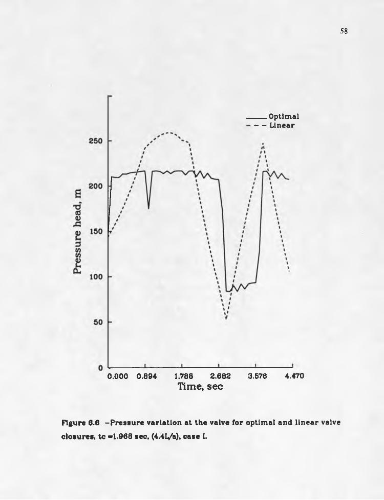
6 .6 Pressure variation at the valve for optimal and linear valve closurestc =1.968 sec (4.4L/a), case I . ........................................................................................58

6 .7 Discharge variation at the valve for optimal valve closure,tc =1.968 sec (4.4L/a), case I..........................................................................................60

6 .8 Maximum and minimum pressures for linear and optimal valve closuresas a function of valve closure time, case II...................................... ............................61

6 .9 Percentage reduction in the dynamic pressure head as a function of valveclosure time, case II.................................................................... 62

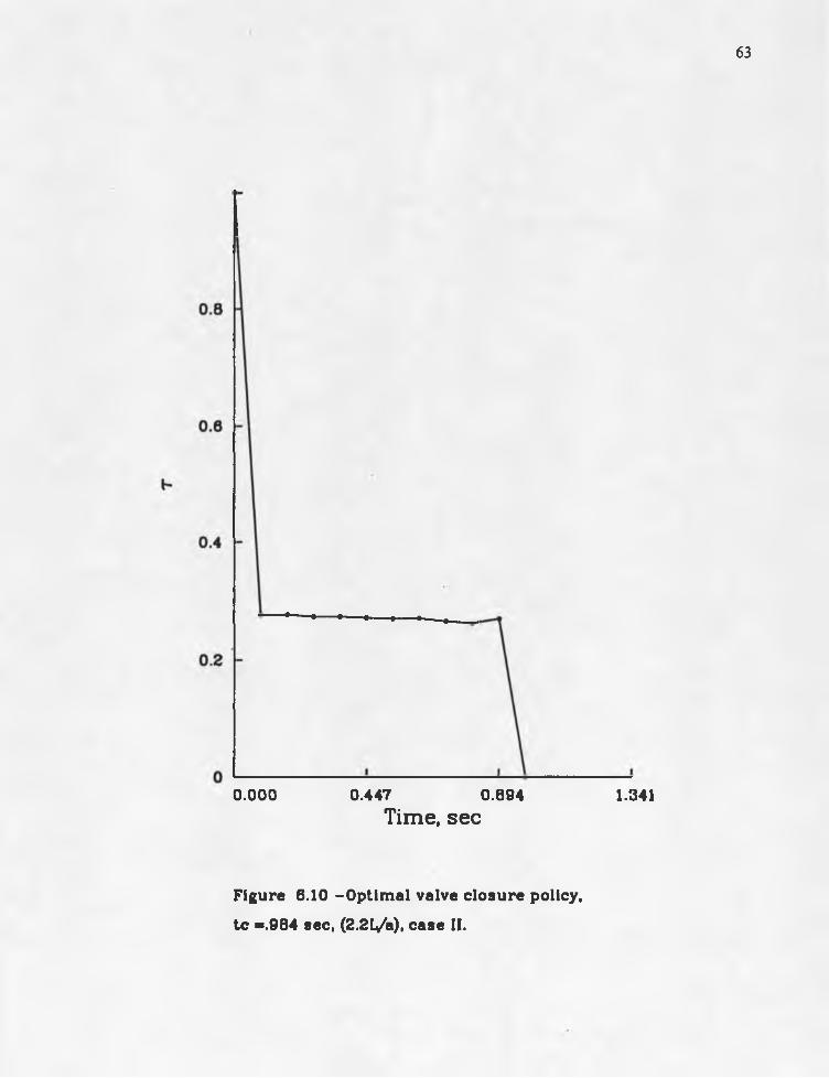
6 .10 Optimal valve closure policy, tc =.984 sec (2.2Ua), case II. . . . . . . 63

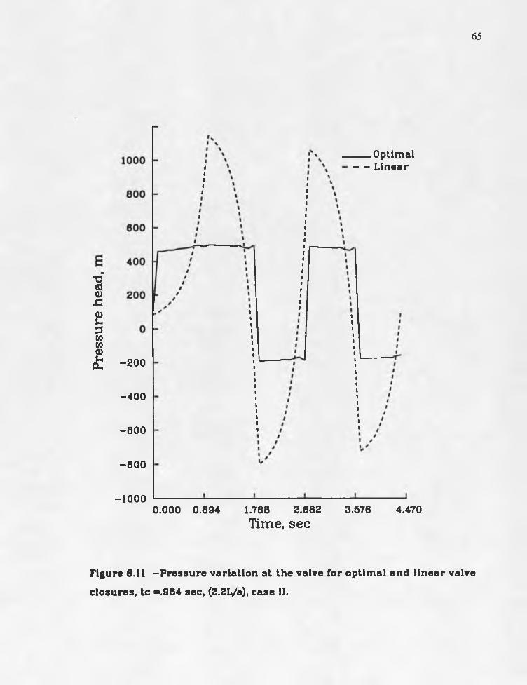
6.11 Pressure variation at the valve for optimal and linear valve closures,tc =.984 sec (2.2L/a), case II. . . .................................. ........................................... 65

6 .12 Discharge variation at the valve for optimal valve closure,tc =.984 sec (2.2L/a), case II........................................................................................... 66

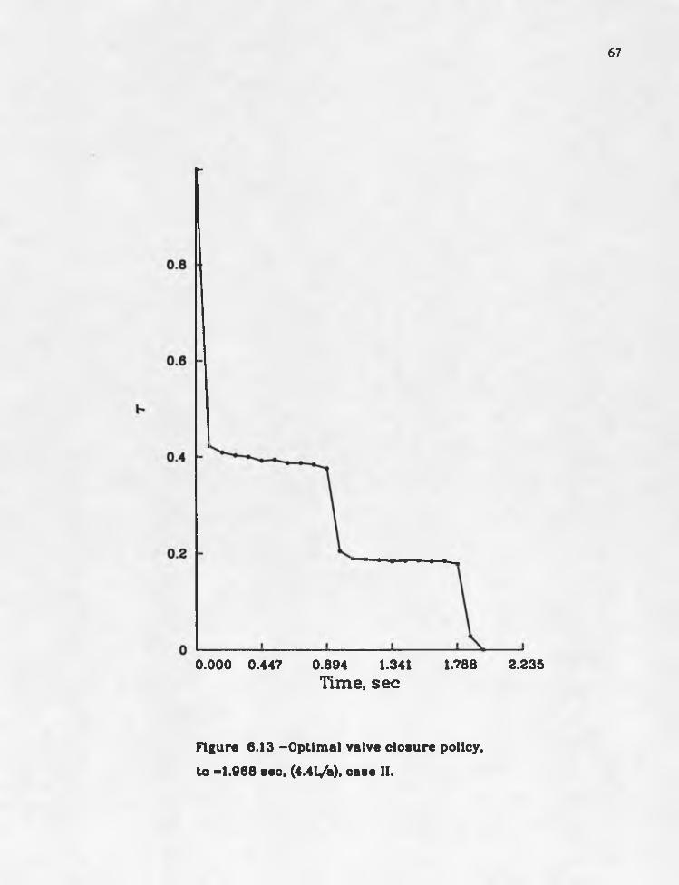
6 . 1 3 Optimal valve closure policy, tc =1.968 sec (4.4L/a), case II. . . . . . 67

6 . 1 4 Pressure variation at the valve for optimal and linear valve closures,tc =1.968 sec (4.4Ua), case II. . . . . ............................. .................................... 69

6 . 1 5 Discharge variation at the valve for optimal valve closure,tc =1.968 sec (4.4L/a), case II. . . . . . . . . . . . . . . . 70

6 .16 Optimal valve closure policy, tc =.984 sec (2.2l7a), case III. . . . . . 71

8

LIST OF ILLUSTRATIONS - Continued

Figure Page

6 . 1 7 Pressure variation at the valve for optimal and linear valve closures,to =.984 sec (2.2L/a), case III. ......................................................... ..... . . . . . 72

6 . 18 Discharge variation at the valve for optimal valve closure,to =.984 sec (2.2L/a), case III.............................................................................................. 74

6 .19 Optimal valve closure policy, to =1.968 sec (4.4L/a), case III................................75

6 .20 Pressure variation at the valve for optimal and linear valve closures,to =1.968 sec (4.4LZa), case III......................... .... ......................................................... 76

6.21 Discharge variation at the valve for optimal valve closure,to =1.968 sec (4.4L/a), case III............................................................................................ 77

6 .22 Maximum and minimum pressures for linear and optimal valve closuresas a function of valve closure time, case III. ......................................................... . 78

6 .23 Maximum and minimum pressures for linear and optimal valve closuresas a function of valve closure time, case IV. . . . . .............................................80

6 .24 Percentage reduction in the dynamic pressure head as a function of valveclosure time, case IV............................................................................ ............................. 81

6 .25 Optimal valve closure policy, tc =.984 sec (2.2L7a), case IV..................................82

6 .26 Pressure variation at the valve for optimal and linear valve closures,tc =.984 sec (2.2L/a), case IV . .............................................................. ........................ 83

6 . 27 Discharge variation at the valve for optimal valve closure,tc =.984 sec (2.2L/a), case IV.. . . .................................................................... 85

6 .28 Optimal valve closure policy, tc =1.968 sec (4.4L7a), case IV. . . . . . 86

6 .29 Pressure variation at the valve for optimal and linear valve closures,tc =1.968 sec (4.4L/a), case IV................................................... ........................... .... .. 87

6 .30 Discharge variation at the valve for optimal valve closure,tc =1.968 sec (4.4lVa), case IV......................................................................................89

9

LIST OF TABLES

Table Page

5.1 Comparison of Maximum Pressures Obtained by Step Valve Closure and

Optimal Valve C lo s u re ............................. ......................... 47

NOEyENCLMytRE

A Cross-sectional area

Ag Opening area of valve

a Speed of wave in the fluid

b side length of simplex

cd Orifice discharge coefficient

D Diameter of pipe

F Objective function value

Fh The highest value of objective function

FI The lowest value of objective function

Fm The second highest value of objective function

f Darcy Weisbach friction factor

g Gravitational acceleration

H Piezometric height

Hmax Maximum pressure head

Hmin Minimum pressure head

Hres Reservoir head

Ht dH/dt

Hx dH/dx

Hv Vapor pressure

L Length of pipe

n number of variables used in simplex

11

n 1 number of reaches in pipe

Q discharge

t time

tc Time of closure of valve

V Velocity

Vx dV/dx

Vt dV/dt

x distance

Ax a small segment of distance

dx thickness of fluid element

a angle of inclination of pipe with x-axis

a l reflection coefficient

p i contraction coefficient

y l expansion coefficient

% parameter used in establishing initial T-time curves

Y specific weight of fluid

X multiplier parameter for partial differential equations

T dimensionless valve opening

Th T-time curve which gives the highest value of objective function

Tm T-time curve which gives the second highest value of objective function

Tl T-time curve which gives the lowest value of objective function

To shear stress

12

ABSTGMCT

Fluid transients (maximum pressure) in a pipeline can be reduced significantly

by using an optimal valve closure. In some situations, the optimal valve closure policy

may result in minimum pressures below the vapor pressure of the fluid. Consequently,

column separation will occur with high pressures in the pipeline that were not taken

into account in analysis of the optimal valve closure policy. Thus it is desirable to

minimize the maximum pressure (Hmax) in a pipeline, subject to the constraint that

the minimum pressure (Hmin) be greater than or equal to a pre-selected pressure, e.g.

the vapor pressure of the fluid (Hv). This is accomplished by changing the objective

function to a minimization of (Hmax-Hmin), with the stipulation that when Hmin < Hv,

the objective function becomes (Hmax-Hv).

The method of characteristics is used to simulate fluid transients in a pipe, and

the simplex method is used to optimize the objective function. A numerical example is

provided to illustrate the valve-closure policies obtained when different objective

functions are used, e.g. minimizing Hmax, maximizing Hmin, and minimizing

(Hmax-Hmin). It is shown that a valve-closure policy can be found that minimizes

Hmax while avoiding water column separation.

13

CHAPTER T

INTRODUCTION .

In steady flow, the velocity at a point in a fluid system does not change with time

whereas in unsteady flow, the velocity will change. Transition flow is the state when

flow conditions are changing from one steady state to another steady state. In pipeline

flow, transient flow and waterhammer are used to describe the unsteady flow.

Sudden disturbances in the flow system, such as changes in valve settings, pump

operation, and changes in reservoir elevation, create changes in pressure head and

velocity. The changes can be positive or negative depending upon the operation of valve

or pump and parameters of pipeline, if the pressure in a closed conduit drops below

vapor pressure of the fluid, cavities referred to as column separation are formed in the

water column.

Severe waterhammer and column separation in a flow system are undesirable as

these can cause damage to the operating system or pipes. Negative pressures should be

increased to slightly higher than the vapor pressure of the fluid to avoid column

separation. It is impossible to completely avoid waterhammer, but it is desirable to

decrease waterhammer effects so that they will not result in damage to the system.

A piping system can be designed to withstand any maximum and minimum

pressures expected to occur during the life of the system but the cost may be

uneconomical. Therefore, various devices are used to avoid undesirable pressure rise

and drop or column separation.

14

The devices commonly used to reduce excessive pressures and avoid column

separation are:

1- Surge tanks

2- Air chambers

3- Valve operating criteria

Transient flow can be controlled by the following operations of a valve.

1- The valve closes or opens in a certain manner to reduce positive and

increase negative pressures.

2- When pressure exceeds a certain level the valve opens to allow rapid

outflow, e.g. a pressure-relief valve.

3- To prevent the pressure from dropping to vapor pressure, the valve opens

to admit air, e.g. air-inlet valves.

Valves that can be operated easily (according to specific instructions) are

worthwhile, considering the savings that would result from improved pipeline design or

control system operation. No extra equipment is required, when a valve operating policy

is adopted to limit the fluid transients. The simplex method is used to optimize the valve

closure for a simple flow system including a reservoir, a pipeline, and a valve. A

computer model is developed which gives the optimal valve closure policy (for a certain

time of closure) to avoid column separation and minimize waterhammer pressure.

15

CHAPTER 2

LITERATURE REVIEW FOR LIMITING PRESSURE TRANSIENTS

In the past several decades, investigators have developed methods to compute

numerically the magnitude of waterhammer transients in pipelines. One of their aims

was to reduce the waterhammer pressure by any appropriate means. In the beginning,

system designers explored how waterhammer pressures changed when arbitrarily

changing the valve-operating policy. Of the policies investigated, they could choose the

policy which gave the least waterhammer pressure.

Streeter (1963) proposed a technique called “valve stroking" to control

waterhammer pressures, i.e. a valve operating policy which limits the pressure rise to

a pre-set maximum without flow reversal and without separation of the fluid column.

He developed equations for closing a valve at the downstream end of a pipeline leading

from a reservoir so that the minimum pressure remains above the steady state values at

all times.

Oriels (1975) studied minimizing waterhammer pressure by closing the valve

in two linear stages, the mode of closure being characterized by the point at which the

valve actuator speed changes. This point was determined by using a simplex search

algorithm, so that for given initial flow conditions and valve closure time, the

waterhammer pressure can be minimized.

Contractor (1983) suggested that waterhammer pressures can be minimized by

operating the valve in an optimally prescribed manner, in a given time of closure. He

used dynamic programming to determine the valve closure policy so that the pressure

16

rise at the valve can be minimized. He also concluded that the benefits of optimal gate

closure are greatest when the time of closure is small (2Ua <tc<3L/a).

Contractor (1985) studied optimal valve closure in two or three stages to

minimize waterhammer pressure rises. The Box-complex method was used to optimize

a valve closure policy for a given time. He also introduced the step valve closure policy.

In this policy, the valve is closed instantaneously to a certain opening and is kept at that

opening for 2l_Za seconds, then it is closed to another opening and so on until the valve is

completely closed. The intermediate openings are determined by using the Box-complex

method.

Sen and Contractor (1986) applied minimax optimization procedure to minimize

the maximum pressure anywhere along the pipeline. Conway (1986) applied the

dynamic programming technique to a series pipeline to determine the optimal

valve-closure policy and concluded that the dynamic programming scheme is sensitive to

pipe configuration, junction location, friction factor, and closure period.

Azoury et al. (1986) studied, for a simple pipeline discharging into free air, the effect

of valve closure policy on waterhammer pressure under friction conditions and

presented a chart that can be used to determine valve schedule for minimum

waterhammer pressure.

Goldberg (1987) proposed a time-optimal valve closure procedure called Quick

Stroking. El-Ansary and Contractor (1988) proposed an optimal valve closure to

minimize waterhammer pressures and stresses in a pipeline. They used the simplex

method for optimizing the valve closure policy.

17

CHAPTER 3

WATERHAIWMER ANALYSIS

The distribution of pressure and velocity in a closed conduit, with flowing water,

depends upon the conditions under which the flow occurs. If the water is considered

incompressible and the flow is steady, the velocity of water remains constant and

Bernoulli's energy equation can be applied at any two sections of the pipe. However,

when the flow is unsteady, i.e. when velocity at each section varies with time, abrupt

pressure changes occur inside the pipe, and Bernoulli's equation is no longer applicable.

These pressure fluctuations are referred to as waterhammer because of the hammering

sound which often accompanies the phenomenon. The flow is called transient flow and is

analysed as follows:

3-1 Partial D ifferen tia l Equations fo r W aterham m er

Two basic differential equations are applied to describe the unsteady flow

through a closed conduit: the equation of motion and the continuity equation. The

following assumptions are made in the derivation of the equations (Chaudhry, 1979).

1. Flow is one-dimensional and the velocity distribution is uniform over the

cross-section of the conduit.

2. Formulae for computing the steady state friction losses in the conduit are valid

during the transient state.

18

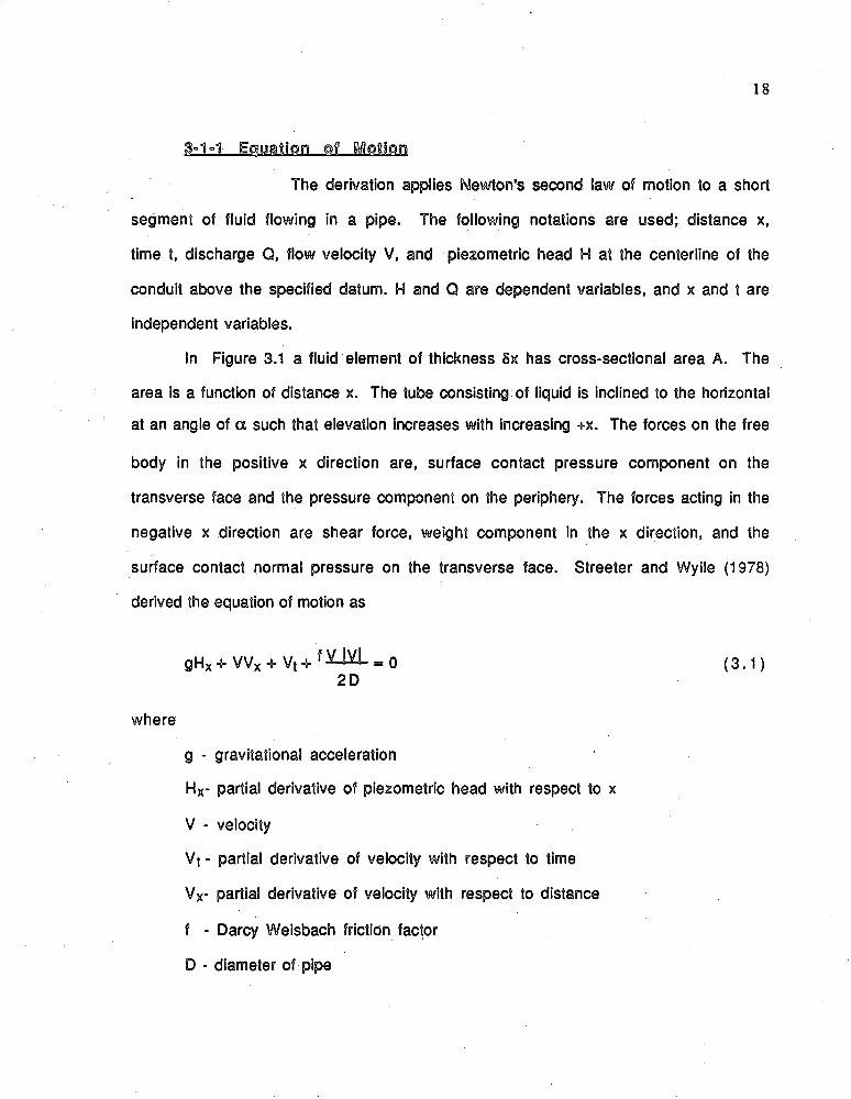
3-1-1 Equation - off R/ilotion

The derivation applies Newton's second law of motion to a short

segment of fluid flowing in a pipe. The following notations are used; distance x,

time t, discharge Q, flow velocity V, and piezometric head H at the centerline of the

conduit above the specified datum. H and Q are dependent variables, and x and t are

independent variables.

In Figure 3.1 a fluid element of thickness Sx has cross-sectional area A. The

area is a function of distance x. The tube consisting of liquid is inclined to the horizontal

at an angle of a such that elevation increases with increasing +x. The forces on the free

body in the positive x direction are, surface contact pressure component on the

transverse face and the pressure component on the periphery. The forces acting in the

negative x direction are shear force, weight component in the x direction, and the

surface contact normal pressure on the transverse face. Streeter and Wyile (1978)

derived the equation of motion as

gHx + VVX + Vt + f = 0 2D

where

g - gravitational acceleration

Hx- partial derivative of piezometric head with respect to x

V - velocity

Vt - partial derivative of velocity with respect to time

Vx- partial derivative of velocity with respect to distance

f - Darcy Weisbach friction factor

D - diameter of pipe

( 3 . 1 )

19

Hydraulic grade li

H-p 5x/2)A 5x

Datum

Figure 3.1 Freebody diagram for application of equation of motion.

20

3°11°% Equation off ConlUnHftv

The control volume of length 8%, in Figure 3.2, is fixed relative to

the pipe. At time t, the net mass inflow Into the control volume will be equal to the rate

of change of mass within the control volume. This is required by the law of conservation

of mass. Wylie and Streeter (1978) give the continuity equation in which H and V are

dependent variables and x and t are independent variables as

VH X + Ht - V Sin cm- &2 Vx = 0 ( 3 . 2 )g

where

V - velocity

Hx - partial derivative of piezometric head with respect to distance x

Ht - partial derivative of piezometric head with respect to time t

V x - partial derivative of velocity with respect to distance x

a - wave speed in the pipe

3-2 Solution of Partial Differential Equations

The dynamic and continuity equations need to be solved simultaneously for

waterhammer or transient flow in a pipeline. They are quasi-linear, hyperbolic, and

partial differential equations. While closed form solution of these equations is

impossible (Chaudhry , 1979), there are numerical techniques to solve these

equations by using computer analysis, such as the characteristics method. In this

method the partial differential equations are transformed into total differential equations

and these latter equations are then solved by a finite difference technique.

Hydraulic grade line

pA(V-u) + [pA(V-u)] ^

pA(V-u

Datum

Figure 3.2 Control volume for continuity equation.

22

3-2-1 The Method of dharaeitetlgftiegs

The two quasi-linear partial differential equations are

transformed into four ordinary differential equations by the method of characteristics.

In the derivation, terms of lower magnitude are dropped. The simplified dynamic

equation and equation of continuity are identified below (Streeter and Wylie , 1979).

Li = qHy + Vt + f V IVl = 0 ( 3 . 3 )2D

l_2 = Ht + a2 Yx = 0 g

( 3 . 4 )

The pair of Equations (3.3) and (3.4) is replaced by a linear combination of equations.

Using X as a linear factor, the equations can be combined as

Li + X L2 = 0 ( 3 . 5 )

gHx + Vt + f V IVI + X [Ht + a2 Vx ] = 0 ( 3 . 6 )2D

Any two real and distinct values of X give two equations in terms of two dependent

variables H and V. If V and H are dependent on x and t.and independent variable x is

permitted to be a function of t, then the derivative of V and H can be written as

d t i = Hx d)L+ Ht ( 3 . 7 )

dt dt

d Y . V x J & L + V t ( 3 . 8 )

dt dt

Equation (3.6) can be replaced by the ordinary differential equation

x d H + d % _ + f y m _ = odt dt 2D

( 3 . 9 )

i f

23

_a_ = L a 2 dt 1 g

The solution of Equation (3.10) gives

( 3 . 1 0 )

X = ± g / 2 ( 3 . 1 1 )

and + a ( 3 . 1 2 )dt

Substitution of these values of X in Equation (3.9) gives two pairs of equations which are

identified as C+ and C* equations.

a. dH+iflL+fvjLyi _ oa dt dt 2D

( 3 . 1 3 )

+ a dt

( 3 . 1 4 )

.e u d tiu 'd S L + f m ^ oa dt dt 2D

( 3 . 1 5 )

d 2 L . - adt

( 3 . 1 6 )

In the x-t plane, these Equations (3.14) and (3.16) are represented by straight lines.

C+ and C* are called characteristic lines along which Equations (3.13) and (3.15) are

valid, as shown in Figure 3.3. This pair of equations now can be written in finite

difference form and solved conveniently with the digital computer.

3-3 The F in ite D ifference Equations

A pipeline is divided into n1 equal reaches of length Ax. The time step

At is the time required by the wave to travel Ax distance and is computed by

24

Characteristic lines

Figure 3.3 Characteristic lines in the x-t plane.

• Upstream boundary ^ Downstream boundary o Interior Section o Initial state

Figure 3.4 Characteristic Grid.

25

— A & ( 3 . 1 7 )

a

At any point on x-t plane in Figure 3.4, say point P, the values of H and V are unique i.e.

the H and V are independent of which characteristic they were approached from

(Watters, 1984). If we construct C+ and C" characteristics through the point, we have

two ordinary differential equations which apply along their respective characteristics.

The differential equations can now be expressed in finite difference form. Equations

(3.13) and (3.15) become (Steeter and Wyile ,1979)

Hp - Ha + a- (Qp - Qa ) + L & l QA|QA| = 0 ( 3 . 1 8 )

gA 2g DA2

Hp - H B " S - (Qp - Q g ) -L M .Q B |Q B | = o ( 3 . 1 9 )

gA 2g DA2

solving equations for Hp

C + : Hp = HA - B(Qp - Qa ) - R(QA |QA|) ( 3 . 2 0 )

C- : Hp = Hb + B(Qp - Qb) + R(QQ|QB|) ( 3 . 2 1 )

whereB = a - ( 3 . 2 2 )

gA

R = l & L ( 3 . 2 3 )

2g DA2

Initially at time t=0, the conditions are steady and the values of H and Q are

known. The problem occurs from != At onward, H and Q are computed for each grid point

along t= At, and then proceeding to t=2 At etc., until a desired maximum time has been

26

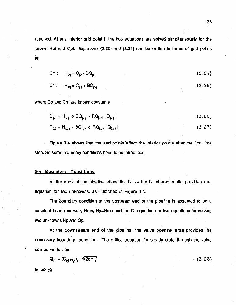
reached. At any interior grid point i, the two equations are solved simultaneously for the

known Hpi and Qpi. Equations (3.20) and (3.21) can be written in terms of grid points9 II o > ( 3 . 2 4 )

C" : Hpj - C y + BQp. ( 3 . 2 5 )

where Cp and Cm are known constants

Cp = Hj i + BQj .j - RQj.-j I ( 3 . 2 6 )

C M = Hk1 " BQi-i-1 + RQi+1 lQi+11 ( 3 . 2 7 )

Figure 3.4 shows that the end points affect the interior points after the first time

step. So some boundary conditions need to be introduced.

3-4 Boundary Conditions.

At the ends of the pipeline either the C+ or the C' characteristic provides one

equation for two unknowns, as illustrated in Figure 3.4.

The boundary condition at the upstream end of the pipeline is assumed to be a

constant head reservoir, Hres, Hp=Hres and the C* equation are two equations for solving

two unknowns Hp and Op.

At the downstream end of the pipeline, the valve opening area provides the

necessary boundary condition. The orifice equation for steady state through the valve

can be written as

Q 0 = (Gd V o ^ ( 3 . 2 8 )

in which

27

Qo - steady state flow

Ho - steady state head at the vah/e

(CdAg)o - the area of the valve opening times the discharge coefficient at steady

state

An equation similar to Equation (3.28) may be written for the transient state as

Qp = (c d A g H ta iA H ) ( 3 . 2 9 )

in which AH is the instantaneous drop in hydraulic grade line across the valve. A

dimensionless parameter T can be defined as

; T . & £ L M(Cd Ag)o

Thus, we get

Q r = Qq_ t V(AH) ( 3 . 3 0 )V(Ho)

T is 1. for steady state flow and 0 for a fully closed valve. By solving Equations (3.24)

and (3.30) for Qp

Qp = - BCv + V{(BCv)2 + 2C\/Cp} ( 3 . 3 1 )

where

Cv= £Qfi^2 ( 3 . 3 2 )2 H0

Hp Can be found from Equation (3.24) or (3.30).

28

CHAPTER 4

OPTIMIZATION

Optimization can be defined as the process of finding the conditions that give the

maximum or minimum value of a function. There is no single method available for

solving all optimization problems efficiently; a number of optimization techniques are

available for solving different types of problems.

Optimization techniques, also known as mathematical programming techniques,

are useful in determining the maximum or minimum of a given function of several

variables for the given set of constraints.

All optimization methods are classified into two general categories as,

1- derivative-free methods

2- gradient methods

The gradient or descent methods require both function and derivative evaluations

while derivative-free, or direct search, methods require function evaluations only. In

general, gradient methods seem to be more effective, due to the added information

provided. If analytical derivatives are available, there is no doubt that a gradient

technique should be used. However, if numerical derivative approximations are utilized,

the efficiency of gradient methods would be approximately the same as that of the

derivative-free methods. The simplex method is one of several widely-used techniques

of derivative-free methods.

29

4=1 The gsHmalaa: meHhedl

The geometric figure formed by a set of n+1 points in n-dimensional space is

called the simplex. When the points are at unequal distances the simplex is called

irregular. In two dimensional space, the number of points are three, and the simplex is

a triangle; in three dimensional space, it is a tetrahedron.

The currently accepted simplex technique is due to Nelder and Mead (1965). The

procedure is an extension of the simplex method by Spendly, et.al., (1962). This

technique accelerates the simplex method and makes it more general. This simplex

method adapts itself to the local landscape, using reflected, expanded, and contracted

points to locate the minimum. Unimodality is assumed, and thus several sets of starting

points should be considered. Derivatives are not required.

This method is clearly applicable to the problem of minimizing a mathematical

function of several variables, having constraints. In the method the simplex adapts

itself to the local landscape, elongating down along inclined planes, changing direction on

encountering a valley at an angle, and contracting in the neighborhood of a minimum, as

shown in Figure 4.1. The criterion for stopping the process depends upon the accuracy

of results needed.

The method can be applied to several kinds of problems unless the function is

discontinuous. It does not require unidirectional searches or any line search techniques.

The method can be applied to non-differentiable functions and when the first partial

derivatives are discontinous. This method contains very simple mathematical operations

and each step is computed using the previous step so that a lot of computer memory is not

required. As the number of the variables increases, the mean number of evaluations for

convergence increases rapidly (Nelder and Mead 1965). Rapid and safe convergence can

30

Figure 4.1 -Typical simplex search in two-dimensions.

31

be achieved by using a maximum number of variables of ten, resulting in efficient use of

computer time.

4-2 M ethodology

In n-dimensional space, n+1 vertices make a simplex. These vertices are

denoted by Ti (i=1,2,.....,n+1). An initial point T1 is selected, with coordinates in

n-dimensional space denoted as (T1,1,T1,2,....... ,T l,n ), and the point must satisfy all the

constraints.

An initial simplex is constructed consisting of the starting point and the following

additional points (Kuester and Mize, 1973).

Tj = T l+ Q, j = 2,3,........n+1

where Q is determined from the following table

j Cl.i (2,j " Cn-1,j Cn.j

2 P q q q

3 q P q q■ " " =

° " a a n

n q q p q

n+1

where

q q q p

p = __h_nV2

[V(n +1) + n -1] (4 .2)

q =

where

bn V I

[V(n +1) -1] (4.3)

n - total number of variables

32

b - side length of simplex, it determines the area of search; as b

decreases, the area of search decreases

After establishing the initial simplex, the function is evaluated at each vertex of

the simplex. Let X and F denote the point and the objective function value respectively.

Th.Tm and Tl are the points of the simplex which give the highest, the second highest and

the lowest values of the objective function. Fh,Fm and FI are the objective function

values respectively, f is the centroid of these points excluding the worst point Th and is

found using the following relation:

n+1

T = 1 /n { % ( V ' M , 4 . 4 )

H

The point, having the highest value of the objective function, is called the worst

point, and is replaced by a new point. The new point is found by the following four

operations. These operations are shown graphically in Figure 4.2.

I - Reflection

The reflected point of Th is located as follows:

T° = ( 1 + a i ) T - a i T h ( 4 . 5 )

where a-j is a positive reflection coefficient and is equal to 1.0. The function value at the

new reflected point is given as F \ If F* lies between Fh and FI, then Th is replaced by

T* and a new simplex is established.

33

dimension, 4) contraction along all dimensions.

34

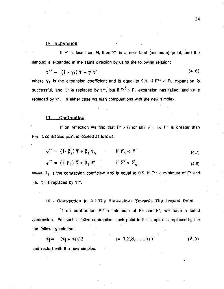
II- Esmanalon

If Fe is less than FI, then X " is a new best (minimum) point, and the

simplex is expanded in the same direction by using the following relation:

% * * = (1 - Y i) T + Y t * (4 6)

where is the expansion coefficient and is equal to 2.0. If Fco < Fl, expansion is

successful, and Th is replaced by T**, but if F*4 > FI, expansion has failed, and Th is

replaced by V . In either case we start computations with the new simplex.

Ill ° C ontraction

If on reflection we find that F* > Fi for all i * h, i.e. Fe is greater than

Fm, a contracted point is located as follows:

t " - (1 -P , ) f+P , t h i fFh<F- (4.7)

t " - (1-P,) f + P, f i f F - < F h (4.8)

where P i is the contraction coefficient and is equal to 0.5. If F14 < minimum of F4 and

Fh, Th is replaced by T44.

IV ° Contraction In All Th® Dimensions Towards The Lowest Point

If on contraction F44 > minimum of Fh and F4, we have a failed

contraction. For such a failed contraction, each point in the simplex is replaced by the

the following relation:

T j= ( T j + T | ) / 2 j= 1,2,3,..... ,n+1 ( 4 .9 )

and restart with the new simplex.

35

The best values of Pi and y-| are those, which converge the simplex fast

towards the minimum. Nelder and Mead (1965) found experimentally that the best

values are 1.0, 0,5 and 2.0 respectively.

4-3 Model Description

T is a dimensionless valve opening (area) used in waterhammer computations.

t = l & L M (4 . 10 )(Cd Ag)o

where

(CdAg)0 -at steady state

(CdAg) -intermediate state

Commonly, 10 points in T-time space are chosen for optimization as these give

rapid convergence (Nelder and Mead ,1965). For very precise results, the number of

points should be the same as the number of computational time steps At in time of

closure of valve. T is the position of the valve opening at different times. For

optimization purposes, the ten positions of % are chosen at equal time intervals within

the time of valve closure, tc. The boundary conditions are that T = 1 at t = 0 and T = 0 at

t = tc. During the optimization procedure, if T is calculated to be greater than 1.0 or

less than 0.0, T is assigned a value of 0.99999 or 0.00001, respectively.

Waterhammer computations use X at time intervals of At (time step), and these

values of T are interpolated from the optimized values of T, which are generally at

larger time intervals, using the natural cubic spline method (SPLINE subroutine).

At = length of pipe/(wave speed'divisions of pipe)

36

The flow chart for the simplex method is given in Figure 4.3, and the flow chart

for the computer model is given in Figure 4.4.

4-4 S a lin e Intem olaSion

A smooth interpolation can be obtained graphically by using some mechanical

means such as french curves or a flexible elastic bar to pass through the desired points.

Cubic spline functions are mathematical functions that analog the flexible elastic bar.

Polynomial equations are used to represent the curves, requiring a smooth transition at

junction points. The construction of cubic spline interpolation function for valve

opening T as a function of time t is given as follows (Hornbeck,1975):

A number of points ti, i = 1...... n, which may not necessarily be evenly spaced,

with their functional value Ti, i = 1......n are given. These points make n nodes and n-1

intervals. For each interval the following cubic equation is used as the interpolating

function between the two nodes.

F(tj) = Tj = a0 + ai tj + &2 tj2 + as tj3 (tj < tj < t j+ i) ( 4 . 1 1 )

There are four unknowns in the Equation (4.11). The (n-1) intervals result in

4(n-1) unknowns, and 4(n-1) equations are required to solve for the unknowns. These

equations are summarized as follows:

- The function F(t) is continous and has continous first and second derivatives at

each of the (n-2) interior nodes resulting in 3(n-2) equations.

- For each node F(tj) = T j i =1,2.... n will give n equations, making the total

number of equations so far. equal to 4n-6.7 -

- Two more equations are needed to determine completely the spline function.

These conditions are achieved by setting F"(ti) = F"(tn)=0. These

37

Pick starting pointsti j=1.2,3,

Evaluate F(t| ) j=1,2,3.....n+1

Calculate centriod of all t's except t

Determine Th»‘cm»3Optimized

Satisfyonstrainti

Calculate reflected point x ________

Evaluate

Replace t by t

Set boundary conditions for t 0.000015T50. 99999Calculate

expansion point t*

S Satisfy ̂Constraints

Calculate contracted point x* ‘using x F <Fh ?y

EvaluateSet boundary conditions for x *0.000015x* <0. 99999 Satisfy

onstrainti Calculate contracted point x using x

Replace x by x* JsF < F , l

Replace x by x* EvaluateSet boundary conditionsfor x *0.00001 ̂ x* <0. 99999

Move points 1/2 the distance towards the

best pointjsF < F, ?v

Figure 4.3 The flow chart of the Nelder and Mead simplex.

Read Pipe Data

Figure 4.4 The flow chart of the Computer Model.

39

conditions make the so-called natural spline and the number of equations

equals 4(n-1).

40

CHAPTER I

MODEL VERIFICATION

The results obtained from the present model are compared with results obtained

by the step-closure policy given by Contractor, (1985). The same basic data are used

for this model, except that the transient computations are made at six equidistant points

along the pipe, whereas in the step-closure policy there are eleven equidistant points.

The time step used in the step-closure program is one half of the time step used in this

model.

The following data are used to verify the model.

pipe length L = 4030.0 ft

pipe diameter D = 0.0833 ft

Darcy Weisbach friction factor f = 0.036

initial velocity Vo = 1.10 ft/sec

(CdAg)0 = 0.000074

fluid wave speed a = 2550.00 ft/sec

reservoir head Hres 140.00 ft

P rob lem #1

The objective of the problem is to determine the optimum valve-closure policy

for a given time of closure; i.e. such that the maximum pressure head anywhere in the

pipeline is reduced to a minimum. As a ten-dimensional space is used in the simplex

model, eleven % curves are needed to start the simplex procedure. Time of closure, tc, is

41

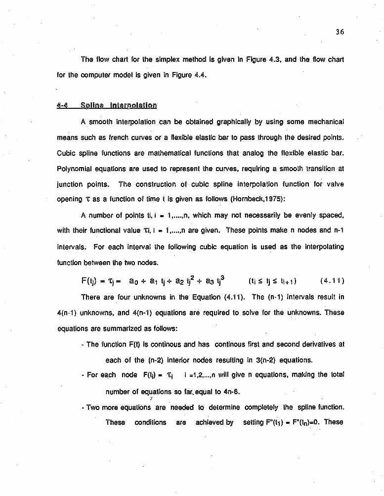
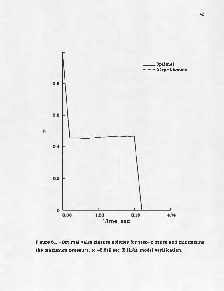
taken to be slightly greater than 2L/a i.e. 3.319 sec. The optimum valve closure policy

obtained is shown in Figure 5.1 and is very close to that given by Contractor (1985).

The pressure variation, at the valve, with linear and optimum valve closures, shown in

Figure 5.2, indicates that the maximum pressure is reduced from 206.3 ft to 165.3 ft

and minimum pressure rises from 85.7 ft to 105.9 ft with the optimal valve closure

policy. The percentage reduction in dynamic pressure is computed as follows:

The steady state pressure at the valve = 105 94 ft

The maximum pressure for linear valve closure = 206.36 ft

The maximum pressure for optimal valve closure = 165.33 ft

2 0 6 .3 6 - 165 .33Percentage reduction in dynamic pressure = --------------------- = 40.86 %

2 0 6 .3 6 - 1 0 5 .9 4

The variation in discharge, when the valve is closed optimally, is shown in Figure 5.3.

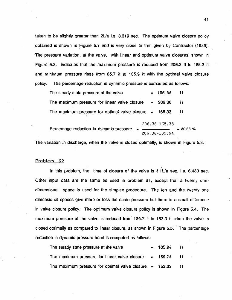
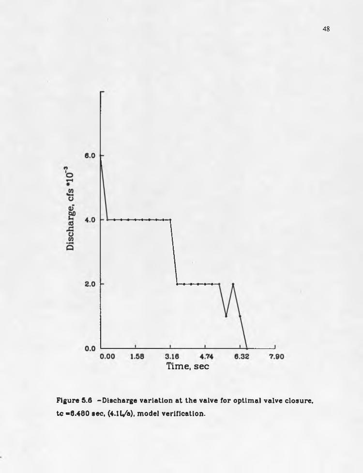
P rob lem 8 2

In this problem, the time of closure of the valve is 4.1 L/a sec. i.e. 6.480 sec.

Other input data are the same as used in problem #1, except that a twenty one-

dimensional space is used for the simplex procedure. The ten and the twenty one

dimensional spaces give more or less the same pressure but there is a small difference

in valve closure policy. The optimum valve closure policy is shown in Figure 5.4. The

maximum pressure at the valve is reduced from 169.7 ft to 153.3 ft when the valve is

closed optimally as compared to linear closure, as shown in Figure 5.5. The percentage

reduction in dynamic pressure head is computed as follows:

The steady state pressure at the valve = 105.94 ft

The maximum pressure for linear valve closure = 169.74 ft

The maximum pressure for optimal valve closure = 153.32 ft

42

___Optimal---- Step-Closure

T im e , se c

Figure 5.1 -Optimal valve closure policies for step-closure and minimizing

the maximum pressure, tc -3.319 sec (2.11/a), model verification.

Pre

ss

ure

he

ad

, ft

43

___Optimal---- Linear

0.000 3.161 6.322 9.483T im e , sec

Figure 5.2 -Pressure variation at the valve for optimal and linear valve

closures, tc -3.319 sec, (2.1l/a). model verification.

44

T im e , sec

Figure 5.3 -Discharge variation at the valve for optimal valve closure,

tc -3.319 sec. (2.1L/&). model verification.

45

___Optimal---- Step-Closure

3.16 4.7T im e , se c

Figure 5.4 -Optimal valve closure policies for step-closure and minimizing

the maximum pressure, tc -6.480 sec (4.1L/a), model verification.

46

----- Optimal---- Linear

0 .000 3.161 6.322 9.483T im e , sec


closures, tc -6.480 sec, (4.1 L/a), model verification.

47

1 6 9 .7 4 - 153 .32Percentage reduction in the dynamic head = -----------------— - = 25.74 %

1 6 9 .7 4 - 105 .94

Figure 5.6 shows the discharge variation at the valve for optimal valve-closure.

Computations were made for different times of closures of the valve. Data in

Table 5.1 show a comparison of the maximum head obtained by the present model and

produced by Contractor (1985).

Table 5.1. Comparision of Maximum Pressures Obtained by Step Valve Closure and Optimal Valve Closure.

Valve Closure I Maximum Pressure Head (ft)Time Linear Valve Optimal Step Optimal

sec L/a Closure Valve Closure Valve Closure

3.319 2.1 208.2 166.3 165.3

6.480 4.1 169.5 155.6 153.3

9.640 6.1 159.5 147.6 149.1

12.801 8.1 153.8 146.3 146.3

Small differences in the results of the two optimal policies may be attributed to

the different time steps used in the two methods. Computations with a smaller time step

should be more accurate than computations with a larger time step.

The percentage reduction in dynamic pressure is plotted against valve closure

time in Figure 5.7. As is clear from Figure 5.7, the highest peak of reduction of 41%

occurs with a valve closure of about 2.2L/a sec. and the second highest peak of reduction

of 25 % occurs at about 4.4173 sec.

48

T im e , se c


tc -6.480 sec, (4.1l/a). model verification.

49

Closure time, L/a sec

Figure 5.7 -Percentage reduction in dynamic pressure head as a

function of valve closure time, model verification.

50

CHAPTER i

COMPUTER IMPLEMENTATION AND RESULTS

A simple pipeline with a constant head reservoir at the upstream end and a valve

at the downstream end is chosen for application of the model. Different cases are studied,

with different flow rates and objective functions. The valve operation, with higher

discharge through It, creates higher pressure variation. These pressure variations are

very often undesirable. The aim is operate the valve so as to reduce the maximum

pressure and to increase the minimum pressure, if it is below the vapor pressure of the

fluid, or to reduce the maximum pressure while keeping the minimum pressure at some

limiting value.

The objective function, which is to be optimized by the simplex, is the key factor

in determining the solution of the problem. It can control only one of the limiting values

at a time; either minimum pressure or maximum pressure in a specified time of valve

closure. Four cases are studied and presented to show how selection of the objective

function changes the nature of the solution.

All four cases that are studied, use the same basic data which are given below:

length of pipe

diameter of pipe

reservoir head

Darcy Weisback friction factor

gravity acceleration g

fluid wave speed

600.00 meters

0.50 meters

150.00 meters

0.018

9.806 meters/sec5

1341.13 meters/sec

51

6°H 1

This is the simplest case in which the steady state velocity of the flow is very

-low. The product of discharge coefficient and cross-sectional area of the valve at steady

state ((CdAg)0) is 0.009. The discharge and velocity through the pipe are 0.5 cu.m/sec. X

and 2.55 m/sec respectively. The objective in this case is to minimize the maximum

pressure head obtained from waterhammer computations. The optimum valve closure

policy obtained from the above computations, does not result in a minimum pressure

lower than the vapor pressure of the fluid.

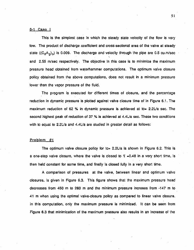
The program is executed for different times of closure, and the percentage

reduction in dynamic pressure is plotted against valve closure time of in Figure 6.1. The

maximum reduction of 62 % in dynamic pressure is achieved at tc= 2.2L/a sec. The

second highest peak of reduction of 37 % is achieved at 4.4L/a sec. These two conditions

with tc equal to 2.2L/a and 4.4L/a are studied in greater detail as follows:

P rob lem #1

The optimum valve closure policy for tc= 2.2LZa is shown in Figure 6.2. This is

a one-step valve closure, where the valve is closed to T =0.48 in a very short time, is

then held constant for some time, and finally is closed fully in a very short time.

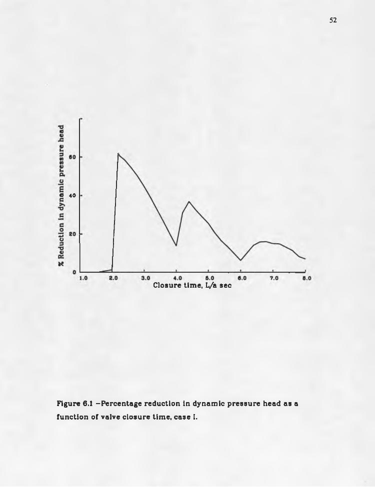
A comparison of pressures at the valve, between linear and optimum valve

closures, is given in Figure 6.3. This figure shows that the maximum pressure head

decreases from 450 m to 260 m and the minimum pressure increses from -147 m to

41 m when using the optimal valve-closure policy as compared to linear valve closure.

In this computation, only the maximum pressure is minimized. It can be seen from

Figure 6.3 that minimization of the maximum pressure also results in an increase of the

52

0 40



function of valve closure time, case I.

53

1.3410.8940.4470 .000T im e , se c

Figure 6.2 -Optimal valve closure policy,

tc -.984 sec, (2.2L/&)’ case I.

Pre

ss

ure

he

ad

,

54

E

400

300

200

100

0

100

_____Optimal— — — Linear

-200 ------------------- '------0.000 0.894

__I_________ i i

1.788 2.682 3.576T im e , s e c

4.470


closures, tc -.984 sec, (2.21/*). case I.

55

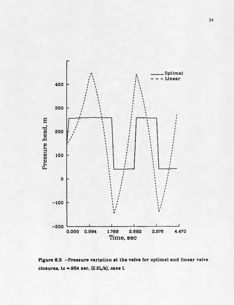
minimum pressure from -146 m to 40 m. Thus, column separation is avoided

simultaneously with reduction of the maximum pressure.

The steady state pressure at the valve = 143.49 m

The maximum pressure resulting linear valve closure = 450.39 m

The maximum pressue resulting optimal valve closure = 259.99 m

450.39- 259.99Percentage reduction in dynamic pressure = ____________ = 62.04 %

450.39- 143.49

The discharge variation at the valve, shown in Figure 6.4, indicates discharge is reduced

only 36 % when the valve is closed to T= 0.52.

Problem #2

The optimum valve-closure policy for time of closure of 4.4L/a sec (1.968 sec)

is shown in Figure 6.5. This is a two step valve closure. In the first step the valve is

closed to T=0.65 in a very short time and is held constant to about 2LZa sec. In the

second step, it is closed to T = 0 .3 2 and is kept constant to about 4L/a sec then finally

closed fully in a very short time.

A comparison of pressure head variation at the valve, with linear and optimal

valve closures, is shown in Figure 6.6. This shows that the maximum pressure is

reduced 42.6 m and the minimum pressure is increased 31.4 m when closing the valve

optimally as compared to linear closing.


The maximum pressure while using linear closure = 258.83 m

The maximum pressure using optimal valve closure* 216.23 m

258.83-216.23Percentage reduction in dynamic pressure = ____________ = 36.93 %

258.83-143.49

56

0 .000 0.447 0.894 1.341T im e , sec


tc -.984 sec, (2.2L/a), case I.

57

1.7881.3410.000 0.447 0.894T im e , se c


tc -1.968 sec, (4.4L/»). case I.

58


4.4702.682 3.5760.000 0.894 1.788T im e , se c


closures, tc -1.968 sec, (4.4L/a). case I.

59

The discharge variation at the valve is shown in Figure 6.7. In the first step, when the

valve is closed to T= 0.65, discharge reduces to 79 %, and in the second step, when the

valve is at T= 0.30, the dischrage is 37 %.

6-2 Case 11

In this case, the steady state area of the valve opening is increased so that

(C(jAg)0 =0.038, resulting in a steady state velocity of 7.80 m/sec and a discharge of

1.532 cu.m/sec. The objective function that was specified was simply minimization of

the maximum pressure. Figure 6.8 shows that as the time of valve closure increases,

the maximum pressure decreases and the minimum pressure increases. This figure also

shows that abrupt changes in pressure occur at specific closure times. These time of

closures are slightly larger than 2L/a, 4L/a and 6L/a sec. As the time of closure

increases, the change in pressure decreases, as shown in Figure 6.8. It is seen that

minimum pressure is higher than the vapor pressure of the fluid, only when time of

valve closure is greater than 6L/a sec.

This program is executed for different times of closure and a graph is plotted of

percentage reduction in dynamic maximum pressure versus valve closure time of

Figure 6.9. The maximum reduction of 65 % is achieved at 4.4l_Za sec, and the second

highest peak of reduction of 61 % is occured at 2.2LZa sec. For a better understanding

and comparison, of the different cases, problems are studied in detail for tc equal to

2.2L/a sec and 4,4L/a sec.

P rob lem #1

The optimum valve closure policy for tc= 2 .2L/a sec (0.984 sec) is shown in

Figure 6.10. This is a one-step valve closure. In cases I and II, the same data are used,

except that in case II the initial valve opening is bigger than in case I. In case I, the

60

0.000 0.447 0.894 1.341 1.788 2.235T im e , sec


tc *1.988 sec, (4.4L/&)' case I.

Pres

sure

hea

d.

61

Optimal

Linear

Hmax1000

Hmax

Hmin

Hmin

1000


Figure 6.8 -Maximum and minimum pressures for linear and optimal

valve closures as a function of valve closure time, case II.

f l 40



function of valve closure time, case II.

63

0 .000 0.447 0.894 1.341T im e , sec


tc -.984 sec, (2.2l/a ). case II.

64

optimum valve closure is at T=0.48 whereas in case II the optimum valve closure is at

about % =0.28.

A comparison of pressures at the valve with linear and optimal valve closures.

Figure 6,11, shows the maximum pressure is reduced from 1144 m to 496 m and the

minimum pressure is increased from -800 m to -190 m.

The steady state pressure at the valve 82.92 m

For linear valve closure

The maximum pressure at the valve = 1144.50 m

The minimum pressure at the valve = -799.89 m

For optimum valve closure



1144.50- 496.97Percentage reduction in dynamic pressure (max) = ______________ = 61.00 %

1144.50- 82.92

-799.89-(-1 90.05)Percentage increase in dynamic pressure (min) =_________ _______= 69.08 %

-799.89 - (82.92)

Figure 6.12 shows the variation in the discharge at the valve. When the valve is closed

to an opening of T= 0.28, the discharge reduces to only 66 %.

P rob lem #2

In this problem the time of closure of the valve is 4.4Ua sec and the optimum

valve-closure is given in Figure 6.13. This is also a two-step valve closure, except that

the valve is closed to 1=0.40 in the first step as compared to 1=0.65 in case I. In the

second step, the valve is closed to 1=0.20 as compared to 1=0.32 in case I. The

computer output is given in Appendix B.

Pre

ss

ure

he

ad

,

65

___ Optimal---- Linear

-2 0 0

-400

—600

—800

-10002.682 3.576 4.4700.000 0.894 1.788

T im e , sec


closures, tc -.984 sec, (2.2L/a), case II.

66

0.000 0.447 0.894 1.341T im e , se c


tc -.984 sec. (2.2L/a), case II.

67

1.788 2.2350.000 0.447 0.894 1.341T im e , se c


tc -1.968 sec, (4.4L/®). case II.

68

A comparison of pressures at the valve with linear valve closure and optimal

valve closure, Figure 6.14, shows that the maximum pressure is reduced from 845 m to

352 m and the minimum pressure increased from -525 m to -50 m.








845.24- 351.92Percentage reduction in maximum pressure = _______ __ = 64.71 %

845.24- 82.92

-525.51-(-49.57)Percentage increase in minimum pressure = ----------------------- = 78.22 %

-525.51-( 82.92)

Figure 6.15 shows that the discharge is 83 % when the valve opening is T = 0.40 in the

first step of valve closure, and in the second step, when the valve opening is T= 0.20 ,

the discharge is 37 %.

6-3 Case II

The same data are used as in case II except that the objective function is

changed to maximization of the minimum pressure. The simplex converges towards

maximum value of the minimum pressure, which is the steady state pressure at the

valve. The valve closure policy, for tc =2.2L/a sec, and the pressure variation at the

valve for linear and optimal valve closures, are shown in Figures 6.16 and 6.17,

respectively. The maximum pressure in Figure 6.17 is much higher than the maximum

Pre

ss

ure

he

ad

,

6 9

___ Optimal---- Linear

-2 0 0

—400

—6003.576 4.4700.000 0.894 1.788 2.6f

T im e , sec


closures, tc -1.968 sec. (4.41/a), case II.

70

1.788 2.2350.000 0.447 0.894 1.341T im e , se c


tc -1.968 sec, (4.4L/&). case II.

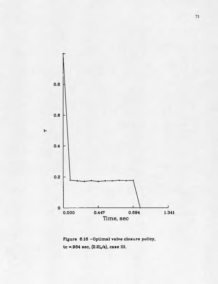
1.3410.447 0.8940.000T im e , sec


tc -.984 sec, (2.2L/a), case III.

Pre

ss

ure

he

ad

,

72

___Optimal---- Linear1000

-2 0 0

-400

—600

—8000.000 0.894 1.788 2.6f

T im e , sec3.576 4.470


closures, tc -.984 sec, (2.2L/a), case III.

73

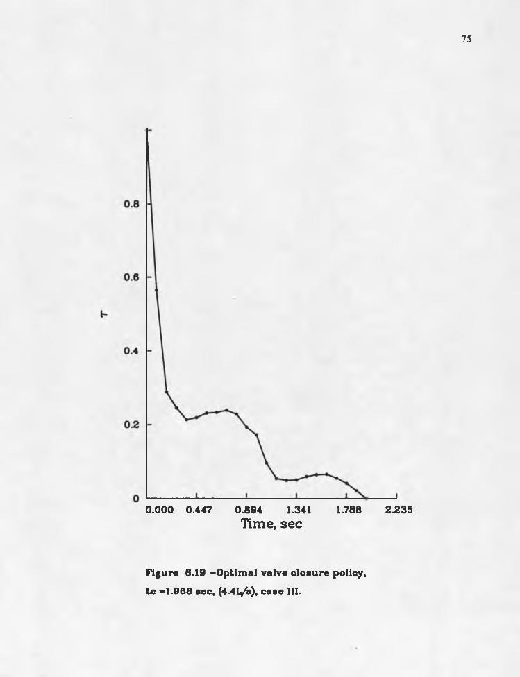
pressure in Figure 6.11. Figure 6.18 shows the discharge variation at the valve.

Figures 6.19 and 6.20 show the valve closure for tc =4.4L/a sec and pressure

-variations for linear and optimal valve closures, respectively. The maximum pressure

in Figure 6.20 is much greater than the maximum pressure in Figure. 6.14. Discharge

variation is shown in Figure 6.21. The maximum and minimum pressures for linear

and optimum valve closures are plotted versus valve closure time in Figure 6.22.

Figure 6.22 shows that optimal closure always raises the minimum pressure to the

steady state pressure at the valve, i.e. 82.9 m, and it is shown as a straight line. The

pattern of change of maximum pressure in Figure 6.22 is strange. As the results are

undesirable the details are not discussed further.

6-4 Case IV

The same data are used in this case as in case II and case III, but the objective

function is different. In case II the objective function used for optimization is

minimization of the maximum pressure irrespective of any value of the minimum

pressure (which, most of the time, was below -10 m, the vapor pressure head). In

case IV the objective function is specified as the minimization of the difference of

maximum and minimum pressures with the constraint that minimum pressure should be

equal to or greater than some limiting value, e.g. vapor pressure at -10 m.

When the simplex tries to minimize the value of the objective function, in the

absence of some limiting value of the minimum pressure, the simplex gives very high

values of maximum pressure and minimum presssure i.e. steady state pressure at the

valve, because at these values their difference is minimum. By introducing the limiting

value of minimum pressure the simplex tries to minimize the difference between

maximum and minimum pressures when the minimum pressure is less than the limiting

74

0.25 -

0.894 1.3410.000 0.447T im e , sec


tc -.984 sec, (2.21/8). case III.

75

0.000 0.447 0.894 1.341 1.788 2.235T im e , sec


tc -1.968 sec, (4.4V®). case III.

Pre

ss

ure

he

ad

,

76


-2 0 0

-400

— 6000.000 0.894 2.682 3.5761.788

T im e , se c4.470


closures, tc -1.968 sec, (4.4^/s), case III.

77

0.000 0.447 0.894 1.341 1.788 2.235T im e , sec


tc ■1.968 sec, (4.4L/a), case III.

Pres

sure

hea

d,

78

1000

E500

0

-6 0 0

-1 0 0 0

Optimal

Linear

Hmax

Umax

Hmin

Hmin



valve closures as a function of valve closure time, case III.

79

value. When the actual minimum pressure is equal to or greater than the limiting value,

the simplex tries to minimize the difference of the maximum pressure and the limiting

value of minimum pressure. By this technique the simplex first tries to increase the

minimum pressure to some limiting value, then it tries to minimize the maximum

pressure while keeping the minimum pressure equal to or greater than the limiting

value.

Figure 6.23 shows the variation of maximum and minimum pressures at the

valve for linear and optimal valve closures. In case II the minimum pressure was less

than the vapor pressure (-10. m) until the time of closure was 6.4L/a sec (shown in

Figure 6.8). Figure 6.23 shows that optimization increases the minimum pressure to

-10. m (limiting value) when the minimum pressure was less than the limiting value

(Figure 6.8). But when the minimum pressure is greater than the limiting value

(-10 m), this case acts like case II.

The program was executed for different times of closure, and a graph of percent

reduction in maximum pressure as a function of valve closure time is shown in

Figure 6.24. This figure shows the maximum pressure reduction of 63 % occurs at

about 4.4L/a sec, and the second highest peak of pressure reduction of 57 % occurs at

about 6.6L/a sec. The following problems are studied in detail for time of closures of

2.2L/a and 4.4LZa sec.

Problem

The optimum valve closure for tc =2.2L/a sec shown in Figure 6.25 is a

one-step valve closure. The valve is closed down to T=0.2, as compared to case ll where

the valve was closed to X=0.28. The pressure variation at the valve for linear and

optimum valve closures, given in Figure 6.26, indicates the maximum pressure is

Pres

sure

hea

d,

80

Optimal

Linear

Hmax1000

Hmax

Hmin

Hmin

1000



valve closures as a function of valve closure time, case IV.

81


function of valve closure time, case IV.

0.000 0.447 0.894 1.341T im e , sec


tc -.984 sec, (2.2L/a), case IV.

Pre

ss

ure

he

ad

,

83


-2 0 0

—400

—600

—800

-10000.000 0.894 1.788 2.61

T im e , sec3.576 4.470


closures, tc -.984 sec, (2.2L/a), case IV.

84

reduced from 1144 m to 586 m and the minimum pressure raised from -800 m to

-10 m.





For optimal valve closure



1144.50- 593.97Percentage reduction in dynamic pressure (H m ax)= ------------- ---------- = 51.86%

1144.50- 82.92

-799.89-(-9.99)Percentage increase in dynamic pressure (Hmin) =— ------------------- = 89:4 %

-799.89- (82.92)

The computation shows that in case IV the percent reduction in maximum

pressure is about 9.11 % less than in case li, but the percent increase in minimum

pressure in case IV is about 20.32 % greater than in case II.

Figure 6.27 shows that the flow at T= 0.20 is 55 % of the steady state flow.

Problem 8 2

Time of closure used in this problem is 4.41/3 sec, and the optimal valve closure

policy is shown in Figure 6.28. Valve closure policy in case IV differs from that in

case II is that at the end of the first step in case IV, the valve is slightly opened from

T= 0.36 to T - 0.42 for a short time. Details of valve closure policies in case II and

case IV are given in Appendices B and C, respectively. .The pressure variation for linear

and optimal valve closures, given in Figure 6.29, shows that maximum pressure

85

0.000 0.447 0.894 1.341T im e , sec


tc -.984 sec, (2.2L/a), case IV.

86

0.000 0.447 0.894 1.341 1.788 2.235T im e , se c


tc -1.968 sec, (4.4L/a), case IV.

Pre

ss

ure

he

ad

,

87


-2 0 0

—400

—6000.000 0.894 3.5761.788 2.8*

T im e , sec4.470


closures, tc -1.968 sec. (4.4L/a), case IV.

88

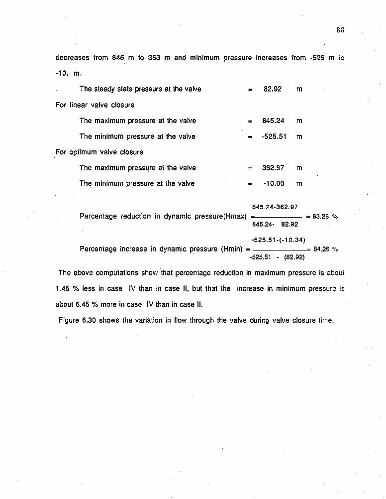
decreases from 845 m to 363 m and minimum

-10. m.

The steady state pressure at the valve


The maximum pressure at the valve

The minimum pressure at the valve


The maximum pressure at the valve

The minimum pressure at the valve

845.24- 362.97Percentage reduction in dynamic pressure(Hmax) =------------------- — = 63.26 %

845.24- 82.92

-525.51-(-10.34)Percentage increase in dynamic pressure (Hmin) = ----------------- ------ -= 84.26 %

-525.51 - (82.92)

The above computations show that percentage reduction in maximum pressure is about

1.45 % less in case IV than in case II, but that the increase in minimum pressure is

about 6.45 % more in case IV than in case II.

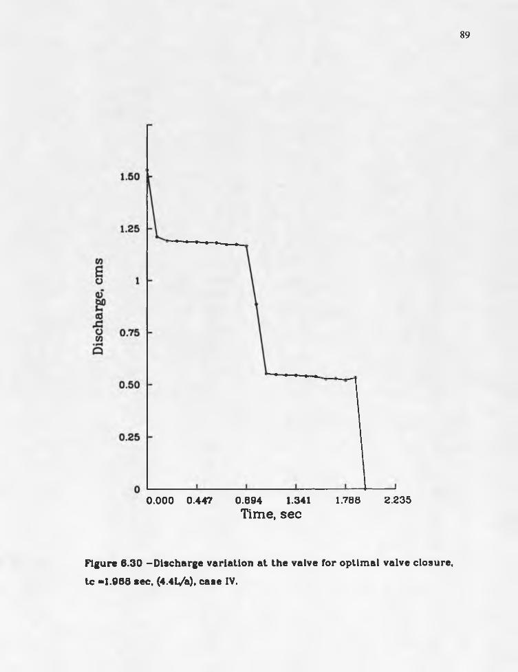
Figure 6.30 shows the variation in flow through the valve during valve closure time.

pressure increases from -525 m to

= 82.92 m

= 845.24 m

= -525.51 m

= 362.97 m

-10.00 m

89

2.2351.7880.894 1.3410.000 0.447T im e , sec


tc -1.968 sec, (4.4L/&). case IV.

90

CHAPTER 7.

DISCUSSION AND CONCLUSION

The change in pressure head during transient flow depends largely on the steady

state velocity of flow; the higher the velocity, the greater the fluctuation in pressure

head. When the maximum pressure is minimized, the minimum pressure also

increases, as shown in Figure 6.8 (case II). Sometimes the steady state velocity in the

pipe is such that when minimizing the maximum pressure, the minimum pressure is

higher than the vapor pressure of the fluid and in such situations there is no concern

about column separation. At other times, the velocity through the pipe is high enough so

that the minimum peressure rises when minimizing the maximum pressure but it is

still lower than the limiting value (i.e vapor pressure). This will cause column

separation, as shown in Figure 6.8 (case II). Column separation is undesirable and

should be avoided.

There are several ways to avoid column separation. One way is to maximize

minimum pressure, but in this case the maximum pressure increases to very high

values which is not desirable. The straight line in Figure 6.22, shows the upper limit

of minimum pressure, that is the steady state pressure at the valve.

A second way is to minimize the difference between maximum and minimum

pressures; this case gives higher values of both maximum and minimum pressures.

Thus, while column separation is avoided by this technique the maximum pressure rises

to very large values.

91

The purpose of this study was to avoid column separation while keeping the

maximum pressure to a minimium. After studying all the cases, it was realized that

optimization should be carried out in two phases. In the first phase, minimize the

difference between the maximum and minimum pressures until the minimum pressure

is equal to the some limiting value (e.g. vapor pressure of the fluid). After the

minimum pressure reaches the limit, a second phase of optimization should minimize

the maximum pressure. The first phase is achieved by minimizing the objective

function {Hmax-Hmin}, when Hmin is < the limiting value (Hv). When Hmin rises to

the limiting value (Hv) the second phase minimizes {Hmax-Hv}. During the second

phase of minimization, Hmin may be > Hv. This objective function is used in case IV.

Figure 6.23 shows that, when compared with case II in Figure 6.8, this technique

increases the minimum pressure to the limiting value and at the same time also

increases the maximum pressure. But the increase in maximum pressure is less than

the increase in the minimum pressure as is clear from the computations in problems

#1 and #2 in case IV.

There are many settings of valve closure, with small differences, which give the

same maximum and minimum pressures. Sometimes we get a wavy pattern of optimal

valve closure which is difficult to apply, practically. When a smaller number of

variables are used for the simplex, the natural cubic spline function gives fluctuations

in the closure policy. Most of the time this can be handled by using the number of

variables equal to the number of time steps in the time of valve closure, as is clear from

valve closure policies discussed in chapter 6. But, sometimes, it is not controlled by

this technique. Then, for practical purposes, the mean line passing through the wavy

line should be used and checked for the transient pressures produced.

92

For future work, more constraints should be given to the t values so that the

optimal valve closure policy will be practicable. In low resistance flows, a constraint

can be given so that T value for the next time step should be equal to or less than the T

value at the previous time step. But for optimal valve closure at high friction flows,

sometimes, the valve must be opened slightly after closing to reduce the maximum

pressure as shown in Figure 6.28.

93

APPENDIX A

LISTING OF THE COMPUTER PROGRAM

This program is written in Fortran language and computes transient pressures

and dischareges at six equidistant locations along the pipe. By default it optimizes the

difference between maximum and minimum pressures when the limiting minimum

pressure is given. The objective function can be changed by changing the lines of

statement number 99 in subroutines HAMMER and HAMMER1 which are (P(I)=HHP-

HLP) and (PSTR-HHP-HLP), respectively. For minimizing the maximum pressure use

PSTR and P(l) equal to HHP. In this case the value of the limiting pressure will not

affect the objective function even it is given as an input. For maximizing the minimum

pressure use P(l) and PSTR equal to -HLP in the lines of statement nuber 99 in

subroutines HAMMER and HAMMER1 and give the value of limiting pressure equal to

very high say 100000 because it helps to sort out the minimum pressure (program

default).

During execution of the program, the highest, the second highest, and the lowest

values of the objective function are shown on the console. When the difference between

the highest and lowest values becomes equal to or less than .005 the execution stops and

asks for another value of side (should be less than .5) for better search dr to prepare

the output file. The value of side should be continuously given till the end results do not

vary much.

* * * * * * * * * * * * * * * * * * * * * * * * * * * * * * * * * * * * * * * * * * * * * * * * * * * * * * * * * * * * * * ****************************************************************

* * PROGRAM HHM V 1 .0 * * * * H RITTEI BY FAIQ HUSSAIET PASHA, 1989 * * * * UNIVERSITY OF ARIZONA * * * * C IV IL ENGINEERING DEPARTMENT * * * * TUCSON ARIZONA 85721 * *

* * TO FIND THE OPTIMUM VALVE CLOSURE THAT MINIM IZE * * * * THE MAX PRESSURE AND AVOID THE COLUMN SEPERATION * ****************************************************************

*********************************************************************** THE PROGRAM IS SUBDIVIDED INTO THE FOLLQUIN SECTIONS *

* i.HHM MAIN PROGRAM CONTROL SUBROUTINES,GENERATE ** IN IT IA L TAU CURVES ** 2 . INPUT SUB INPUT DATA ** 3 . SPLINE! SUB FOR INTERPOLATION ** 4 . HAMMER SUB COMPUTE UATERHAMMER ** BY STREETER 6 UYILE ** 5 . SORT SUB SORTING OBJECTIVE FUNCTION ** 6 . OPTIMIZE SUB USING SIMPLEX BY NELDER 6 MEAD

* 7.SPLIN E2 SUB FOR INTERPOLATION ** 8 . HAMMER! SUB COMPUT UATERHAMMER ** 9.HAMMER2 SUB COMPUTE & URITE DOWN UATERHAMMER***********************************************************************

*********************************************************************** NUM

CONSTANTS AND VARIABLES

- NO. OF EQUAL PIPE SEGMENTS

***

* SIDE - ALLOCATE SEARCH AREA FOR SIMPLEX ** ALPHA - REFLECTION CO-EFFICIENT FOR SIMPLEX ** BETTA - CONTRACTION CO-EFFICIENT FOR SIMPLEX ** GAMMA - EXPANSION CO-EFFICIENT FOR SIMPLEX ** NO - ROM DIMENSION OF MATRIX ** NOO - COLUMN DIMENSION OF MATRIX ** DT - TIME STEP ** TC - TIME OF CLOSURE OF VALVE ** N - NO. OF STEPS IN TC *0 NOS - NO. OF N-DIMENSION IN TAU-TIME SPACE *

o PP - PO U T I I TAU-TIME SPACE USED FOR O PTIM IZATIO I ** * * * * * * * * * * * * * * * * * * * * * * * * * * * * * * * * * * * * * * * * * * * * * * * * * * * * * * * * * * * * * * * * * * *

REAL T A U (30 ,50 ),P (30 ),P L ,P H ,P H ,TA U S T R (S O ),T A U D S T R (50 ), » PP(30,30)„DH,PPDSTR(SO )

INTEGER J „K ,L ,M ,N ,K M ,K L ,K H ,1 0 0 ,1 0 ,1 0 5

COMMON. C, ALENGTH, D IA , DF, G, HR,CDA, TC, TMAX, HUM, IP R , HLPP

CALL INPUT (NOS)

IPR =1HUM =5SIDE = .5ALPHA =1.BETTA = .5GAMMA =2.

DT =ALENGTH/(NUM*C)N = IN T (TC /D T)+1I =1+1 10 =30 100 =50

C NO. OF POINTS USING IN SIMPLEX SHOULD BE =OR<TAU POINTS DH =TC /(B0S+1)IF (D H .LT .D T) HOS=TC/DT

C IN IT IA L CURVES ARE GENERATING P P ( i . l ) = 1 .0 P P (1 ,N 0S + 2 )= 0 .0

DO JJ=2,N0S+1 P P (1 ,J J )= .0 END DO

C CUE1 AND CUES ALLOCATE THE SEARCH AREA FOR THE SIMPLEX.

13 CUE! =S ID E *((N O S+1)* * . 5 + N 0 S - l) / (N 0 S * 2 * * .5 )CUES = S ID E *((N 0 S + l) t ‘6 .5 - l) /(N 0 S < -2 < ‘* . 5 )

DO I I = 2 ,NOS+1

P P ( I I ,1 ) = 1 .01 P P ( I I ,0 0 3 + 2 )= 0 .0

DO JJ = 2 ,003+ 1 IF ( I I . E Q . J J ) THEM P P (II,J J )= P P (1 ,JJ )+ C T JE 1 ELSEP P (II,J J )= P P (1 ,JJ )+ C T JE 2 END IF END DO

END DO

C TAU POINTS ON THE IN IT IA L CURVES ARE FOUND OUT USING THE SPLINE C SUBROUTINE

DO IN I =1 ,103+1CALL SPLINE1(DN, DT, H, NO, NOO, PP, T A U ,IN I, NOS)END DO

C HAMMER SUBROUTINE IS CALLED TO FIND OUT THE HATERHAMMER TRANSIENT

DO I=1 ,N 0S +1CALL HAMMER(TAU,NO,NOO,N,DT,I,P)END DO

C TAU CURVES ARE SORTED OUT WHICH GIVE THE HIGHEST, SECOND HIGHET C AND THE LOWEST FUNCTION VALUES.

17 CALL SORT(P,NO,NOO,N,KH,KM,KL,PH,PM,PL,HOS)PRINT » , PH,PM,PL

CALL OPTIM IZE(N, NO, NOO,KH, KM, K L , PP, ALPHA, DT, P L , PH, * PM, P , GAMMA, BETTA, TAUSTR, TAUDSTR, DN, PPDSTR, NOS)

IF (P H -P L .L E ..0 0 5 ) GO TO 18 GO TO 17

18 P P (1 ,1 ) =PPDSTR(1)

DO JJ =2,N0S+2 P P (1 ,JJ)=P P D S TR (JJ) END DOWRITE (<■,») ' Hmax Hmid Hmin 3

97

WRITE (<=,*) ‘ GIVE EITHER THE REDUCED VALUE OF SIDE (< .S ) OR ZERO'

C SIDE VALUE ALLOCATE THE SEARCH AREA FOR OPTIMUM VALUE. KEEP 01 REDUCIIG C THE SEARCH AREA FOR BETTER RESULTS U IT IL THERE IS 00 CHAIGE 10 THE C OPTIMUM VALUE.

READ (*„=>) SIDE IF (S ID E .E Q .O ) GOTO 19 GOTO 13

C OUTPUT F IL E IS PREPARING

19 CALL HAMMER1(TAUSTR,N00,N ,DT,P1)CALL HAMMER1(TAUDSTR, NOO, N, DT, P2)IF (P 1 .G E .P 2) THENCALL HAMMERS(TAUDSTR, NOO, 0 , DT)ELSECALL HAMMERS(TAUSTR, NOO, I , DT)END IFSTOPEND

C * * * * * * * * * * * * * * * * * * * SUBROUTINE INPUT * * * * * * * * * * * * * * * * * * * * * * * * * * * * * * * *C THIS SUBROUTINE IS USED TO PREPARE INPUT DATA FOR THE PROGRAM.C EACH TIME IT REQUIRES NEW DATA SET.c**********************************************************************

SUBROUTINE INPUT (NOS)

COMMON C, ALENGTH, D IA , DF, G, HR, CDA, TC, TMAX, HUM, IP R , HLPP REAL C, ALENGTH, TC, TMAX,DIA, DF, G, HR, CDA, HLPP INTEGER NOS

WRITE ( * , 1 0 )10 FORMAT( ' WAVE SPEED IN FPS OR MPS = ' )

READ ( * , * ) C

WRITE ( * , 1 1 )11 FORMAT ( ' LENGTH OF THE PIPE IN FT OR M = ' )

READ ( * , * ) ALENGTH

WRITE ( * , 1 2 )12 FORMAT ( ' DIAMETER OF THE PIPE (FT OR M) = ’ )

13

14

15

16

17

18

19

20

3230

98

READ (< -„* ) D IA

WRITE ( * , 1 3 )FORMAT ( ' DARCEY HEISBACH FRICTIOH FACTOR = ' )READ ( * , * ) DF

WRITE ( * , 1 4 )FORMAT ( ' HEAD I I RESERVOIR (FT OR M) = ' )READ ( * , * ) HR

WRITE ( * , 1 5 )FORMAT ( • PRODUCT OF DISCHARGE AND AREA (CdA) = ' )READ ( * , * ) CDA

WRITE ( * , 1 6 )FORMAT ( ' GRAVITATIONAL ACCELERATION g (FT/SS OR M /S S )= ') READ ( * , * ) G

WRITE ( * , 1 7 )FORMAT (» TIME OF CLOSURE OF VALVE (SEC) = ' )READ ( * , * ) TC

WRITE ( * , 1 8 )FORMAT ( ' MAXIMUM TIME TO WHICH COMPUTATIONS NEED (S E C )= ') READ ( * , * ) TMAX

WRITE ( * , 1 9 )FORMAT ( ' NO.OF n-DIMENSIONS IN SIMPLEX (PREFERABLY 1 0 ) = ') READ ( * , * ) NOS

WRITE ( * , 2 0 )FORMAT 0 MINIMUM PRESSURE HEAD YOU WANT (FT OR M) = ’ )READ ( * , * ) HLPP

WRITE ( * , 3 0 ) C, ALENGTH, D IA , DF, HR, CDA, G, TC, TMAX, NOS, HLPP FORMAT 0 THE FOLLOWING VARIABLES ARE USED IN THIS PROGRAM:V

* ) 1. WAVE SPEED = ' ,F 8 .2 /* > 2 . LENGTH OF PIPE = ' , F 8 . 2 /0 > 3 . DIAMETER OF PIPE = ' , F 8 . 4 /0 > 4 . DARCEY HEISBACH FACTOR = ’ ,F 8 .6 /* > 5 . HEAD IN RESERVOIR = ' ,F 8 .2 /o » 6 . CdA = ’ ,F 8 .6 /0 9 7 . g = ' , F 8 . 3 /

65

31

41

42

43

44

45

46

47

48

49

50

51

99

* ' 8 . TIME OF CLOSURE OF VALVE = \ F 8 . 3 /<- ' 9 . MAXIMUM TIME = ' ,F 8 .3 /* ' 10 . n-DIMENSIONS = ' , 1 4 /* ' 11. MIHIMUM PRESSURE HEAD = \ F 8 . 3 /* ' ENTER THE NUMBER OF THE VALUE TO CHANGE OR 0 TO CONTINUE'/)

READ ( * , 6 5 ) IANS FORMAT (1 2 )IF (IAN S .E Q .O ) GOTO 60 WRITE ( * , 3 1 )FORMAT (» ENTER THE VALUE ' / )GOTO (4 1 ,4 2 ,4 3 ,4 4 ,4 5 ,4 6 ,4 7 ,4 8 ,4 9 ,5 0 ,5 1 ) IANS

READ ( * , * ) C GOTO 32

READ ( * , * ) ALENGTH GOTO 32

READ ( * , * ) D IA GOTO 32

READ ( * , * ) DF GOTO 32

R E A D (* ,* ) HR GOTO 32

READ ( * , * ) CDA GOTO 32

READ ( * , * ) G GOTO 32

READ ( * , * ) TC GOTO 32

READ ( * , * ) TMAX GOTO 32

READ ( * , * ) NOS GOTO 32

READ ( * , * ) HLPP

100

GOTO 32

60 URXTE (*,30)C ,ALENG TH,D IA,DF,HR„CDA»G ,TC„TM AX, HQS, HLPP RETURI END

* * * * * * * * * * * * * * * * * * * * * * * * * * * * * * * * * * * * * * * * * * * * * * * * * * * * * * * * * * * * * * * * * ** * * * * * SUBROUTINE SPLINE! * * * * * * o* THIS SUBROUTINE IS USED TO FIND OUT THE TAU POINTS FROM <■* THE GIVEN CURVES. EQUATIONS ARE SOLVED BY GUASS E LIM IN A - *» TION METHOD. *******************************************************************

SUBROUTINE SPLINE1(DN,DT,N,NO,NOO, PP, TAU, I N I , NOS) REAL M A T(30,30),M A TR (30),TA U (N O ,N O O ),G (30),PP (N O ,N O )

* ,D N ,D T ,T ,C 0F F ,P 01 ,P 02 ,P 03INTEGER J , L , I , N, M, NO, NOO, I N I , NOS

P P ( IN I ,1 )= 1 .0 P P (IN I,N 0 S + 2 )= 0 .0 J =1DO I = l.NOS

IF ( J . N E . l ) THEN M A T (I.J ) = 1 .0 ELSEM A T ( I.J ) = 0 .0 END IFM A T ( I ,J + l) =4 .IF (J.NE.NOS)THEN M A T ( I ,J + 2 ) = l .0 ELSEM A T (I,J + 2 ) = 0 .0 END IFM ATR(I) = 6 .0 < - (P P ( IN I,J + 2 ) -2 .0 * P P C lN I ,J + l)+

* P P ( IN I,J ) ) / (D N < - * 2 .0 )J =J+1

END DO

M =1DO I = 1 ,HOS

101

C0FF=M AT(I,H+1)M A T (I.M ) ■ M A T(I.H )/C 0F F M A T (I, M+1 )=MAT( I , H + l) / COFF MAT( I , M +2)=M AT(I, M+2)/COFF

M ATR(I) =MATR( I ) / COFFIF ( I .E Q .IO S )

M A T(I+1,M +1) MATCI+1,M+2) M A T (I+ l,M + 3 )

M ATR(I+1)M =M+1

101 END DO

GO TO 101

=M A T (I+1 ,M + 1)-M A T (I,M + 1)= M A T (I+ l.M + 2 )-M A T (I,M + 2 )= M A T (I+ l,M + 3 )-M A T (I,M + 3 )

=MATR(1 + 1 )-MATR( I )

DO J =1,N0SG (N 0S+2-J) =M ATR (N 0S+1-J)/M AT(N 0S+1-J,N 0S+2-J)

* -G (N 0S + 3 -J )«M A T (N 0S + l-J ,N 0S + 3 -J )END DO

T =0 L —1T A U ( IN I . l ) = 1 .0 T A U (IN I,N ) = 0 .0

DO J = 2 ,N -1T=T+DTLL=LIF (T.GT.LODN) LL=L+1 IF (T .G T .(L + 1 )*D N ) LL=L+2 IF (T .G T .(L + 3 )*D N ) LL=L+3

L=LL

P 0 1 = G (L ) /6 .0 * ( (L *D H -T )* *3 /D N -D N * (L *D ff-T ) )P 0 2 = G (L + 1 ) /6 .0 * ( (T - (L -1 ) * D N )* * 3 /D N -D N * (T - (L -1 ) * D N ) )P03=PP ( I N I . D * (L *D N -T ) /DHP04=PP( I N I , L+1 ) * ( T - ( L - 1 ) *DH)/DMT A U ( I I I , J)=P01+P02+P03+P04

102

IF (TAU(I1I„J).GT.1.0) TAU(m,J) = . 9999999 IF ( T A O d l l , J) . LE.0 .0) TAU(m„J)=. 0000001

END DO RETURN END

* * * * * * * * * * * * * * * * * * * * * * * * * * * * * * * * * * * * * * * * * * * * * * * * * * * * * * * * * * * * * * * * * * * * ** * * * * * * * * * * * * * SUBROUTINE HAMMER * * * * * * * * * * * * ** THIS IS TAKEN FROM STREETER & WYLIE AND IT COMPUTES THE ** UATERHAMMER TRANSIENTS AT EACH POINT OF THE PIPE AFTER EVERY** TIME STEP. **********************************************************************

SUBROUTINE HAMMER(TAU, NO, NOO, H, DT, I , P)

INTEGER L ,M ,N S ,M ,IDIMENSION H P (ll) ,Q P (1 1 ),H (1 1 ),Q (1 1 ),T A U (N O ,N O O ),P (N O )COMMON C, ALENGTH. D IA ,D F , G, HR, CDA, TC, TMAX, HUM,IPR, HLPP

NS=NUM+1R=DF«ALENGTH/(2. *G *D IA * *S * . 7854<-<‘2<-FL0AT(NUM) )B = C /(G *.7 8 5 4 *D IA *D IA )

C FIND STEADY STATE FLOW AND STORE IN ITIALVARIABLES

Q0=SQRT(2,*G*CDA*CDA*HR/(R*FL0AT(NUM)*2.*G*CDA*CDA+1. ) )HHP=0HLP=HLPPDO 20 M=1,NSE (M )=E R -(M -1)*R *Q 0*Q 0IF (H (M ).G T.H H P) THEMHHP = H(M)END IFIF (H (M ).L T .H L P ) HLP=H(M)

20 q(M)=qocvp=.5*qo*qo/H(NS)T=0.K=0L=1

103

30 GO TO 4040 T=T+DT

L = L + iIF (T.GT.TMAX) GO TO 99

C C0MPUTATI01 OF INTERIOR POINTS DO 50 H=2, HUMCP=H(M-1 )+ Q (M -l) * (B -R *ABS( Q (M -1 ) ) )CM=H(M+l)-Q(M+1 ) * (B-R*ABS(Q(M +1 ) ) )HP(M)= . 5 * (CP+CM)IF (HP(M ).GT.HHP) THEN HHP-HP(M)END IFIF (H P (H ).L T .H L P ) THEN HLP=HP(H)END IF

50 Q P(M )=(HP(M )-C M )/BC BOUNDARY CONDITIONS

HP(1)=HRQ P (1)=Q (2) + (H P (1 )-H (2 )-R < ‘Q (2 )*A B S (Q (2 ) ) ) /B IF (T -T C ) 5 5 ,6 0 ,6 0

55 C V=TAU (I, L )*T A U ( I , L)*CVPIF (CV.LT.O .O )THEN CV=0.END IF GO TO 70

60 T A U ( I ,L )= 0 .CV=0.

70 CP=H(NUM) +Q (N U M )*(B -R *ABS(q(N U M )))

AA =C V **2*B **2+C V *C P *2 .IF (A A .L T .O .O ) CV =0 .

qP(NS)=-CV*B+SqRT(CV*CV*B*B+CV*CP*2.)EP(NS)=CP-B*qP(NS)IF (HP(HS).G T.HHP) THEN HHP=HP(NS)END IFIF (H P (N S ).LT .H LP ) THEN HLP=HP(NS)END IFDO 80 M =i,HSH(M)=HP(M)IF (H (M ).G T.HH P) THEN HHP=H(M)

104

BID IFIF (H (H ).L T .H L P ) THEEHLP=H(fOEND IF

80 Q(M)=QP(M)K=K+1IF (K /IP R « IP R -K ) 4 0 ,3 0 ,4 0

99 P ( I ) =HHP-HLPRETURN END

* * * * * * * * * * * * * * * * * * * * * * * * * * * * * * * * * * * * * * * * * * * * * * * * * * * * * * * * * * * * * * * * * ** * * * * * * * * * * * SUBROUTINE SORT * * * * * * * ** THIS FIND OUT THE CURVE OF THE HIGHEST OBJECTIVE FUNCTION** VALUE AND SIMILLARLY THE SECOND HIGHEST AND THE MINIMUM. * * * * * * * * * * * * * * * * * * * * * * * * * * * * * * * * * * * * * * * * * * * * * * * * * * * * * * * * * * * * * * * * * * *

SUBROUTINE SORT(P, NO, NOO, N, KH, KM, K L , PH, PH, P L, NOS) REAL P(NO)PH = P (1 )KH =1

DO I = 2.N0S+1IF (P H .G E .P (I))T E E NPH=PHELSEP H = P (I)KH =1 END IF END DO

PL=100000000

DO I = l.N O S + l IF ( P L .L E .P ( I ) ) THEN

PL = PL ELSE PL = P ( I )K L= I END IF

BID DOPM =-100000000 DO I = 1 ,I0 S + 1

IF ( I.E Q .K H ) THEN GOTO 16 END I F .IF (P (I) .G E .P M ) THEN PM = P ( I )KM =1 END IF

16 END DORETURN END

* * * * * * * * * * * * * * * * * * * * * * * * * * * * * * * * * * * * * * * * * * * * * * * * * * * * * * * * * * * * * * * * * ** * * * * * * * * SUBROUTINE OPTIMIZE * * * * * * * * * * ** THIS CONVERGES THE OBJECTIVE FUNCTION TO A MINIMUM POINT ** IT USES THE SIMPLEX BY NELDER & MEAD. *******************************************************************

SUBROUTINE OPTIM IZE(N, NO, NOO, KH, KM, K L , PP, ALPHA, DT,* PL,PH,PM,P,GAMMA, BETTA, TAUSTR, TAUDSTR, DH, PPDSTR, NOS)

INTEGER H,KM, K L , IP R , KH, NO, NOO, NOS

REAL TAUBAR(SO).TAUSTR(NOO),TAUDSTR(NOO),PP(NO,NOO)* , P L»PH, DT, ALPHA, GAMMA, BETTA. C, ALENGTH, D IA , DF, G, HR, CDA* „P P D S TR (50),P P STR (50),PP B A R (S O ),TA U (30,S 0),* P(NO),PM,TC,TMAX,HLPP

COMMON C.ALENGTH, D IA , DF, G, HR, CDA, TC, TMAX, NUM, IP R , HLPP

DO JJ = 2,N0S+1SUM=0.0 DO I =1,N0S+1

SUM =P P (I,JJ)+S U M END DOPPBAR( J J ) = ( SUM-PP(KH, J J ) ) / (NOS)

END DO

DO JJ =2,N0S+1P P S TR (JJ)=P P B AR (JJ)-ALP H A*(P P(KH .JJ)-P PB A R (JJ))

IF (PPSTR (JJ).LE .O .O )TH EH P P S T R (JJ)= 0 .000001 END IFIF (P P S T R (JJ). G E .1 .0 ) THEN P PS TR (JJ)= .99999999 END IF

END DO

P PSTR (1)=1.0PPSTR(N0S+2)=0.0

CALL SPLINE2 (DN, N , PPSTR, TAUSTR, DT, NO, NOO, NOS)

CALL HAMMER1(TAUSTR,NOO,N.DT.PSTR)

IF (P S TR .LT .PL) THEN

DO JJ =2,H0S+1PPDSTR(JJ)=PPBAR(JJ)+GAMMA*(PPSTR(JJ)-PPBAR(JJ)) IF (P P D S TR (JJ).LE .0 .0 )TH E N PPDSTR(JJ)=0 .000001 END IF

IF (P P D S TR (JJ). G E .1 .0 ) THEN P PD S TR (JJ)= .99999 END IF

END DO

PPDSTR(1)=1.0 PPDSTR(N0S+2)=0.0

CALL SPLINE2 (DN, N, PPDSTR, TAUDSTR, DT, NO, NOO, NOS)

CALL HAMMER!(TAUDSTR, NOO, N, DT, PDSTR)

IF (PDSTR.LT.PL) THEN DO JJ =2,N0S+1

PP(KH ,JJ)=PPDSTR(JJ) END DO P(KH)=PDSTR ELSEDO JJ =2 ,103+1

107

P P(KH ,JJ)=P P STR (JJ)END DO P(KH)=PSTR END IF ELSEIF (PSTR.GE.PM) THEN IF (PSTR.GE.PH) THEN DO JJ= 2 ,N 0 S + iPPDSTR( JJ)=PPBAR( JJ)+ B E T T A *(P P (K H ,JJ )-P P B A R (JJ)) IF (P P D S TR (JJ).LE .O .O ) THEN P PD S TR (JJ)=0.000001 END IF

IF (P P D S T R (JJ ).G E .l.O ) THEN P PD STR (JJ)=.99999

END IF END DO ELSEDO JJ =2,H0S+1PPD STR (JJ)=PPBAR(JJ)+BETTA*(PPSTR (JJ)-PPBAR(JJ)) IF (PPDSTR(JJ).LE.O .O )THEN P P D S T R (JJ )-.000001 END IF

IF (P P D S T R (JJ).G E .1 .0 ) THEN P PD STR (JJ)=.99999 END IF

END DO END IF

CPPDSTR(1)=1.0 PPDSTR(N0S+2)=0.0

CCALL SPLINE2 (DN, N , PPDSTR, TAUDSTR, DT, NO, NOO, NOS)

CALL HAMMER1(TAUDSTR, NOO, N , DT, PDSTR)

IF (PSTR.GE.PH) THENPHH =PHELSEPHH =PSTR END IFIF (PDSTR.LE.PHH) THEN DO JJ = 2.N0S+1 PP(KH, J J ) =PPDSTR( J J )

108

BID DOP(KH)=PDSTRELSE

DO I = 1,H0S+1 IF ( I .E Q .K L ) THEM GOTO 20 ELSEDO JJ= 2 ,H 0 S + iP P ( I ,J J ) = ( P P ( I ,J J ) + P P ( K L ,J J ) ) /2 END DO

END IF

CALL SPLINE1 (D N ,D T ,N ,N 0„N 008PP8T A U ,I,N 0 S ) CALL HAMMER (TAU8N08N008N8DT8I 8P)

20 END DOEND IF ELSEDO JJ = 2„N0S+1 PP(KH8JJ)=PPSTR (JJ)END DOPP(KH81 )= 1 .0PP(KH 8 NOS+2)= 0 .0P(KH)=PSTREND IFEND IFRETURNEND

* * * * * * * * * * * * * * * * * * * * * * * * * * * * * * * * * * * * * * * * * * * * * * * * * * * * * * * * * * * *

SUBROUTINE SPLINE2 (DN,N,PP,TAU,DT,NO,NOO,NOS)

REAL M A T(30 ,30) ,HATR(30) ,TAU(NOQ) ,G (3 0 ) .PP(NO') , * D N »D T„T,C 0FF,P01,P02,P03

INTEGER J , L , 1 ,0 ,1 1 ,NOS

J =1DO I = l.NOS

IF ( J . H E . l ) THEN

109

M T ( I „ J ) = 1 .0 ELSEM A T ( I,J ) = 0 .0 END IFM T ( I . J + 1 ) =4 .IF (J.NE.IO S)THEM M A T (I,J + 2 )= 1 .0 ELSEM A T (I,J + 2 ) = 0 .0 END IFM ATR (I) = 6 .0 * (P P (J + 2 ) -2 .0 » P P (J + l)+

* P P ( J ) ) / (D N * * 2 .0 )J =J+1

END DO

H =1DO I = 1 ,NOS

COFF=MAT( I , M+1)M A T (I,M ) =M AT(I,M )/CO FF M A T (I,M + 1 )= K A T (I,M + 1 )/C 0F F HAT( I , M+2)=MAT( I , M+2) /GOFF

M ATR(I) =MATR(I)/COFF IF (I.E Q .N O S ) GO TO 101

M A T(I+1,M +1) M A T(I+1,M +2) M AT(I+1„M +3)

M ATRCl+l)H =H+1

101 END DO

= M A T (I+ l,M + i) -M A T (I ,M + l) =HAT(1 + 1 ,M+2) -MAT( I , M+2) = M A T (I+ l,M + 3 )-M A T (I,M + 3 )

=MATR(1 + 1 )-MATR( I )

DO J =1,N0SG (1 2 -J ) =MATR(HOS+1-J) /MAT(NOS+1 - J , H 0S+2-J)

* -G (N 0S +3-J) ■J'MAT (NOS+1 -J , N0S+3-J )END DO

T =0 L =1T A U (l) = 1 .0 TAU(H) = 0 .0

DO J = 2 ,0 -1T=T+DTLL=LIF (T .G T .L *D H ) LL=L+1 IF (T .G T .(L + 1 )« D N ) LL=L+2 IF (T .G T .(L + 2 )*D H ) LL=L+3 L=LL

P O l= G (L ) /6 .0 * ( (L * D 0 -T )* * 3 /D 0 -D 0 * (L * D 0 -T ) ) P O 2 = G (L + 1 ) /6 .O * ( (T - (L -1 ) * D 0 )* * 3 /D 0 -D 0 * (T - (L -1 ) * D 0 ) ) P 03=P P (L)* (L *D N -T )/D H P04=PP(L+1)<=(T-(L-1)<-DN)/DH TAU(J)=P01+P02+P03+P04

IF (T A U (J ) .G T . l.O ) T A U (J )= .9999999 IF (T A U (J ).L E .O .O ) T A U (J )= .0000001

END DO RETURN END

* * * * * * * * * * * * * * * * * * * * * * * * * * * * * * * * * * * * * * * * * * * * * * * * * * * * * * * * * * * * * *

SUBROUTINE HAMMER1(TAUSTR, NOO, N , DT, PSTR)

INTEGER L ,H ,N S ,N ,I,N U MREAL H P ( ll) ,q P ( l l) ,H ( l l) ,Q ( l l) ,P S T R ,T A U S T R (H O O ) ,H L P COMMON C, ALENGTH, D IA , DF, G, HR, CDA, TC, TMAX, NUM, IP R , HLPP

HS=NUM+1R =D F*A LE N G TE /(2 .*G *D IA **5*.7854**2*FL0A T(M U M ))B=C /(G *.78S4<>D IA*D IA)

C FIND STEADY STATE FLOW AND STORE INITIALVARIABLESQ0=SQRT(2. *G*CDA*CDA*HR/(REFLOAT(NUM)* 2 . *G*CDA*CDA+1. ) ) HHP=0.

Ill

HLP=HLPP DO 20 11=1,MS

H (M )=H R -(M -1)*R *Q 0*Q 0 IF (H (M ).G T.HH P) THEM HEP = H(M)

END IFIF (H (M ).L T .H L P ) HLP=H(M)

20 Q(M)=QOCVP=.5*Q 0*Q0/H(NS)T=0.K=0L=1

30 GO TO 4040 T=T+DT

L=L+1IF (T.GT.TMAX) GO TO 99

C COMPUTATION OF INTERIOR POINTS DO 50 M=2,NUMCP=H (M -1 )+Q (M -1) <■ (B-R* ABS (Q (M -1) ) ) CM=H(M+1)-Q(M+1)*(B-R*ABS(Q (M + l)))HP(M)= . 5 * (CP+CM)IF (HP(M ).G T.HHP) THEM HHP=HP(M)END IFIF (H P(M ).LT.HLP)THEH HLP=HP(M)END IF

50 QP(M)= (H P (M )-C M )/BC BOUNDARY CONDITIONS

HP(1)=HRQ P C l)= Q (2 )+ (H P (l) -H (2 )-R « Q (2 )« A B S (Q (2 ) )) /B IF (T -T C ) 5 5 ,6 0 ,6 0

55 CV=TAUSTR(L) <-TAUSTR(L) *CVPIF (C V .LT .O .O ) THEM CV=0.END IF GO TO 70

60 TAUSTR(L)=0.CV=0.

70 CP=H(NUH) +Q(MUM)*(B-R*ABS(q(MUM)))

AA =CV062.*B<‘*2.+CV<‘CP*2.IF (A A .L T .O .O ) CV=0. qP(MS)=-CV*B+SqRT(CV*CV*B*B+CV*CP*2.)

H P(IS )=C P -B *qP (H S)IF (H P (IS ).G T .H H P ) THEI HHP=HP(HS)EHD IFIF (H P (H S ).LT .H LP ) THEI HLP=HP(HS)END IF DO 80 1 = 1 ,IS H(M)=HP(M)IF (H (H ).G T .H H P ) THEI HHP=H(M)BID IFIF (H (M ).L T .H L P ) THEN HLP=H(M)END IF

80 q(M)=QP(M)K=K+1IF (K /IP R * IP R -K ) 4 0 ,3 0 ,4 0

99 PSTR =HHP-HLPRETURN END

* * * * * * * * * * * * * * * * * * * * * * * * * * * * * * * * * * * * * * * * * * * * * * * * * * * * * * * * * * * * * * *

SUBROUTINE HAMMERS(TAUSTR,1 0 0 ,1 ,DT)

INTEGER L ,M ,N S ,1 , 1 , NUM

REAL H P ( l l ) , q P ( l l ) , H ( 1 1 ) , q ( l l ) , PSTR, TAUSTR(NOO),HLP

COMMON C, ALENGTH, D IA , DF, G, HR, CDA,TC, T H A I, NUM, IP R , HLPP

CHARACTER*15 OUTFILE

WRITE ( * , * ) 'WRITE THE NAME OF THE OUTPUT F IL E 'READ ( * , ' (A ) ' ) OUTFILEOPEN(3 1 ,STATUS*' NEW' ,FILE=OUTFILE)

TAU STR (l) = 1 .IS=IUM+1R=DF*ALENGTH/(2. *G * D IA * * 5 * . 7854**2<-FL0AT(IU M ))

B=C/ (G*. 7854<‘DIA*DIA)C FIHD STEADY STATE FLO'H AMD STORE IMITIALVARIABLES

Q0=SQRT(2. *G*CDA<-CDA<‘HR/(REFLOAT (MUM) *2. *G*CDA*CDA+1.) )HHP=0.HLP=10000000 DO 20 M=1,MS

H(M)=HR-(M-i)<=R*QO*qO IF (H(M).GT.HHP) THEM HEP = H(M)END IFIF (H(M).LT.HLP) HLP=H(M)

20 q(M)=qocvp=.s*qo*qo/H(Ms)T=0.K=0L=1WRITE(32,26)

26 FORMAT(///' TIME PRESSURE TAU ')WRITE(31,25) C ,ALEMGTH,DIA,DF,HR,H(MS),qO,CDA,TC,G ,TMAX,DT

* ,B,NUM,IPR25 FORMAT(' C,ALEMGTH, DIA,DF=’,2F8.1,2F8.4/' HR, HO, qO ='

* .2F8.2.F8.3/* » CDA, TC,,F8.7,F8.3/,G,TMAX,DT,B=,,F8.3,F8.1,F8.5,2X,F10.2/* MUM, IPR='* ,213//' HEADS AMD DISCHARGES ALONG THE PIPE'//’ TIME X/L* 0. .2 .4 .6 .8 1. TAU’)

30 WRITE (31,35)T,(H(M),M=l,NS),TAUSTR(L),(q(M),M=l,HS)35 FORMAT (1H F7.3.5H H=,6F8.2,F7.3/10X,3H q=,6F8 .3)40 T=T+DT

L=L+1IF (T.GT.TMAX) GO TO 99

C COMPUTATION OF INTERIOR POINTS DO 50 M=2,NUMCP=E(M-l)+q(M-l)*(B-R*ABS(q(M-l)))CM=H(M+1)-Q(M+1)*(B-R*ABS(q(M+1)))HP(M)=.5*(CP+CM)IF (HP(M).GT.HHP) THEM HHP=HP(M)END IFIF (HP(M).LT.HLP) HLP=HP(M)

50 qP(M)=(HP(M)-CM)/B C BOUNDARY CONDITIONS

HP(1)=HRQP(l)=q(2)+(EP(l)-H(2)-R*q(2)*ABS(q(2)))/B

IF (H P (l) .G T .H H P ) HHP=HP(1 )IF (H P ( l) .L T .H L P ) HLP =HP(1)IF (T -T C ) 5 5 ,6 0 ,6 0

55 CV=TAUSTR(L) <-TAUSTR(L) <-CVPIF (C V .L T .0 .0 ) THEI CV=0.END IF .GO TO 70

60 TAUSTR(L)=0.CV=0.

70 CP=H(NUM) +Q(NUM )*(B-R*ABS(Q(NUM )))

AA = C V **2 . * B * * 2 . +CV*CP*2.IF (A A .L T .O .O ) CV=0.qP(NS)=-CV*B+SQRT(CV*CV*B*B+CV*CP*2.)EP(NS)=CP-B*qP(NS)IF (HP(NS).G T.HHP) THEN HHP=HP(NS)END IFIF (H P (N S ).LT .H LP ) HLP =HP(NS)DO 80 M=1,NS H(M)=HP(M)IF (H (H ).G T .H H P ) THEN HHP=H(M)END IFIF (H (M ).L T .H L P ) HLP=H(M)

80 q (M )=qp(M )K=K+1IF (K /IP R * IP R -K ) 4 0 ,3 0 ,4 0

99 PSTR =HHP-HLPPRINT *,HHP,HLP CLOSE (3 1 )RETURNEND

Q * * * * * * * * * * * * * * * * * * * * * * * * * * * * * * * * * * * * * * * * * * * * * * * * * * * * * * * * * * * * * * *

115

APPENDIX B

COMPUTER INPUT AND OUTPUT FOR CASE II, te=4.4L/a

The objective function in this case is to minimize the maximum pressure. The

following input data are used.

wave speed = 1341.14 m/sec

length of pipe = 600.00 m

diameter of pipe 0.50 m

Darcy Weisbach friction factor = 0.018

head in reservoir = 150.00 m

CcA, = 0.038

g = 9.806 m/sec'

time of closure of valve 1.968 sec

maximum time = 4.5 sec

n-dimensions = 19

limiting minimum pressure head = -10.00 m

Limiting minimum pressure head does not play any role in the

optimization because of the objectve function. The following is the computer output.

116

CpALEUGTH, DXA,DF= 1341.1 600.0 0.5000 0.0180HR, HO, QO = 150.00 82.92 1.532CDA, TC.0380000 1.968G,TMX,DT,B= 9 .806 4 .5 0.08948 696.54

HUM, IPR= 5 1

HEADS AMD DISCHARGES ALONG THE PIPE

TIKE X/L= 0. .2 .4 .6 .8 1. TAU0.000 H= 150.00 136.58 123.17 109.75 96.33 82.92 0.000

Q= 1.532 1.532 1.532 1.532 1.532 1.5320.089 H= '1 5 0 .0 0 136.58 123.17 109.75 96.33 296.78 0.423

Q= 1.532 1.532 1.532 1.532 1.532 1.2250.179 H= 150.00 136.58 123.17 109.75 307.78 308.27 0 .409

Q= 1.532 1.532 1.532 1.532 1.229 1.2090.268 H= 150.00 136.58 123.17 318.80 319.15 315.70 0.403

Q= 1.532 1.532 1.532 1.232 1.213 1.2050.358 H= 150.00 136.58 329.85 330.06 326.53 318.90 0 .400

Q= 1.532 1.532 1.236 1.216 1.209 1.2010 .447 H= 150.00 340.92 340.99 337.39 329.70 327.78 0 .392

Q= 1.532 1.239 1.220 1.212 1.204 1.1950.537 H= 150.00 351.95 348.27 340.53 338.52 326.26 0 .394

Q= 0.952 1.223 1.216 1.208 1.199 1.1980.626 H= 150.00 158.99 351.38 349.28 337.01 334.94 0 .387

Q= 0.921 0.932 1.212 1.202 1.201 1.1920.716 H= 150.00 151.21 161.65 347.79 345.63 335.19 0.387

Q= 0.912 0.912 0.921 1.205 1.196 1.1920.805 E= 150.00 152.71 149.39 159.66 345.88 340.60 0 .384

Q= 0.904 0.901 0.908 0.917 1.196 1.1910.895 H= 150.00 148.20 150.79 149.20 156.27 348.46 0 .376

q= 0.891 0.900 0.897 0.902 0.915 1.1800 .984 H= 150.00 148.12 148.03 147.50 153.44 343.09 0.205

q= 0.896 0.887 0.893 0.895 0.889 0.6401.074 H= 150.00 149.82 144.88 152.25 333.20 351.94 0.189

q= 0.883 0.889 0.885 0.881 0.622 0.5971.163 H= 150.00 146.76 153.99 329.44 349.55 351.40 0 .188

q - 0.883 0.881 0.877 0.614 0.591 0.5931.253 H= 150.00 154.14 330.19 350.09 347.57 351.00 0.186

q= 0.880 0.871 0.612 0.589 0.585 0.5861.342 H= 150.00 332.28 349.07 348.22 351.53 348.91 0 .184

q= 0.859 0.612 0.585 0.583 0.584 0.5801.432 H= 150.00 343.80 350.22 350.51 349.56 350.42 0 .185

q= 0.347 0 .574 0.583 0.580 0.578 0.5831.521 H= 150.00 168.56 345.25 351.54 349.41 347.03 0.185

117

Q= 0.293 0.319 0.569 0.578 0.579 0.5791.611 E= 150.00 152.14 170.55 344.18 349.02 349.37 0.183

Q= 0.292 0.290 0.316 0.568 0.579 0.5761.700 H= 150.00 152.02 151.75 168.70 344.17 347.67 0 .184

q= 0.286 0.288 0.289 0.317 0.566 0.5781.790 H= 150.00 149.62 150.23 152.42 168.02 347.34 0.178

Q= 0.285 0.286 0.290 0.288 0.318 0.5591.879 H= 150.00 148.21 150.29 149.59 156.24 329.98 0 .028

Q= 0.286 0.286 0.284 0.290 0.282 0.0841.968 H= 150.00 150.67 147.59 154.11 311.33 351.94 0 .000

Q= 0.288 0 .284 0.287 0.278 0.057 0.0002.058 H= 150.00 149.37 154.48 309.10 349.59 351.27 0 .000

Q= 0.282 0.289 0.278 0.054 -0 .0 0 3 0.0002.147 H= 150.00 153.80 310.66 349.73 349.03 347.23 0 .000

0= 0.289 0.276 0.056 -0 .0 0 3 -0 .0 0 3 0.0002 .237 H= 150.00 311.06 348.84 350.57 347.38 346.79 0 .000

Q= 0.270 0.057 -0 .0 0 4 -0 .0 01 0.000 0.0002.326 E= 150.00 344.83 350.96 346.49 348.33 347.53 0 .000

q= -0 .174 , -0 .0 1 0 0.000 -0 .0 01 0.002 0.0002.416 H= 150.00 190.00 342.48 348.72 346.64 349.88 0 .000

q= -0 .2 9 0 -0 .2 3 2 -0 .0 0 7 0.003 -0 .0 01 0.0002.505 H= 150.00 147.89 187.91 342.63 350.27 345.75 0 .000

q= -0 .2 8 9 -0 .2 8 6 -0 .2 28 -0 .0 0 7 0.001 0.0002.595 H= 150.00 148.00 148.27 189.60 341.74 350.66 0 .000

q= -0 .2 8 2 -0 .2 8 5 -0 .2 8 6 -0 .2 3 0 -0 .0 0 6 0.0002 .684 H= 150.00 150.38 149.78 147.61 190.14 337.72 0 .000

q= -0 .2 81 -0 .2 8 2 -0 .2 8 7 -0 .2 8 4 -0 .2 3 0 0.0002 .774 H= 150.00 151.77 149.72 150.40 143.83 29.93 0 .000

q= -0 .2 8 2 -0 .2 8 3 -0 .2 81 -0 .2 8 7 -0 .2 78 0.0002.863 H= 150.00 149.34 152.38 145.94 -9 .5 8 -4 9 .6 2 0 .000

q= -0 .2 8 5 -0 .2 81 -0 .2 8 4 -0 .2 7 5 -0 .0 5 7 0.0002.953 H= 150.00 150.62 145.58 -7 .3 7 -4 7 .2 9 -4 9 .0 6 0 .000

q= -0 .2 7 9 -0 .2 8 5 -0 .2 7 5 —0.054 0.003 0.0003.042 H= 150.00 146.24 -8 .9 1 -4 7 .4 4 -4 6 .8 5 -4 4 .9 7 0 .000

q= -0 .2 8 6 -0 .2 7 3 -0 .0 56 0.003 0.003 0.0003.132 H= 150.00 -9 .3 1 -4 6 .5 6 -4 8 .3 8 -4 5 .1 2 -4 4 .6 4 0.000

q= -0 .2 6 7 -0 .0 5 6 0.004 0.001 0.000 0.0003.221 H= 150.00 -4 2 .6 0 -48 .77 -4 4 .2 4 -4 6 .1 7 -4 5 .2 7 0 .000

q= 0.172 0.010 0.000 0.001 -0 .0 0 2 0.0003.311 H= 150.00 110.45 -40 .28 -4 6 .5 6 -4 4 .3 9 -4 7 .7 0 0.000

q= 0.287 0.229 0.007 -0 .0 0 3 0.001 0.0003 .400 H= 150.00 152.09 112.51 -4 0 .4 3 -4 8 .0 9 -4 3 .5 1 0 .000

q= 0.285 0.283 0.226 0.007 -0 .0 01 0.0003 .490 H= 150.00 151.97 151.71 110.84 -3 9 .5 5 -4 8 .4 8 0 .000

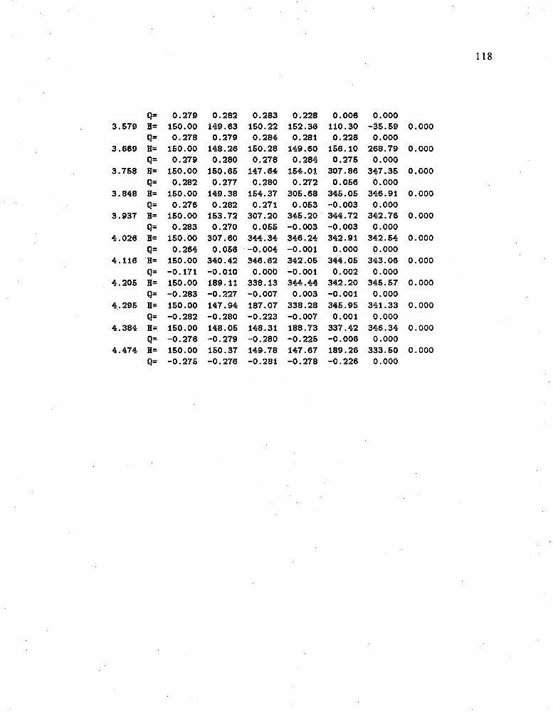
118

Q= 0.279 0.282 0.283 0.228 0.006 0.0003.579 H= 150.00 149.63 150.22 152.36 110.30 -3 5 .5 9

Q= 0.278 0.279 0.284 0.281 0 .228 0.0003.669 H= 150.00 148.26 150.28 149.60 156.10 268.79

Q= 0.279 0.280 0.278 0 .284 0.275 0.0003.758 H= 150.00 150.65 147.64 154.01 307.86 347.35

Q= 0.282 0.277 0.280 0.272 0.056 0.0003.848 H= 150.00 149.38 154.37 305.68 345.05 346.91

Q= 0.276 0.282 0.271 0.053 -0 .0 0 3 0.0003.937 H= 150.00 153.72 307.20 345.20 344.72 342.76

Q= 0.283 0.270 0.055 -0 .0 0 3 -0 .0 0 3 0.0004 .026 H= 150.00 307.60 344.34 346.24 342.91 342.54

Q= 0.264 0.056 -0 .0 0 4 -0 .0 01 0.000 0.0004.116 H= 150.00 340.42 346.62 342.05 344.05 343.06

Q= -0 .1 71 -0 .0 1 0 0.000 -0 .0 01 0.002 0.0004.205 H= 150.00 189.11 338.13 344.44 342.20 345.57

Q= -0 .2 8 3 -0 .2 2 7 -0 .0 0 7 0.003 -0 .0 01 0.0004 .295 H= 150.00 147.94 187.07 338.28 345.95 341.33

Q= -0 .2 8 2 -0 .2 8 0 -0 .2 23 -0 .0 0 7 0.001 0.0004 .384 H= 150.00 148.05 148.31 188.73 337.42 346.34

Q= -0 .2 7 6 -0 .2 7 9 -0 .2 80 -0 .2 2 5 -0 .0 0 6 0.0004 .474 H= 150.00 150.37 149.78 147.67 189.26 333.50

Q= -0 .2 7 5 -0 .2 7 6 -0 .2 81 -0 .2 7 8 -0 .2 2 6 0.000

0 .000

0.000

0.000

0.000

0.000

0 .000

0 .000

0 .000

0 .000

0.000

0.000

119

APPENDIX C

COMPUTER INPUT AND OUTPUT FOR CASE IV, te=4.4L/a

The same data, as used in Appendix B, are used for case IV (minimizing the

difference between maximum and minimum pressures while limiting the minimum

value). But in this case the limiting minimum pressure head (input) plays an

important role. Following is the computer output.

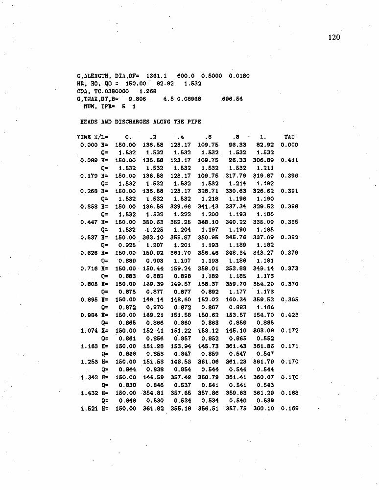
120

C„ALEffGTH, DIA,DF= 1341.1 600.0 0 .5000 0.0180HR, HO, QG = 150.00 82.92 1.532CDA, TO.0380000 1.968G,TMAX,DT,B- 9 .806 4 .5 0.08948 696.54

Him, IPR= 5 1

HEADS AHD DISCHARGES ALOHG THE PIPE

TIME X/L= 0. .2 .4 .6 .8 1.0.000 H= 150.00 136.58 123.17 109.75 96.33 82.92

Q= 1.532 1.532 1.532 1.532 1.532 1.5320.089 H= 150.00 136.58 123.17 109.75 96.33 306.89

Q= 1.532 1.532 1.532 1.532 1.532 1.2110.179 E= 150.00 136.58 123.17 109.75 317.79 319.87

Q= 1.532 1.532 1.532 1.532 1.214 1.1920.268 H= 150.00 136.58 123.17 328.71 330.63 326.62

Q= 1.532 1.532 1.532 1.218 1.196 1.1900.358 H= 150.00 136.58 339.66 341.43 337.34 329.52

q= 1.532 1.532 1.222 1.200 1.193 1.1860.447 H= 150.00 350.63 352.25 348.10 340.22 335.09

q= 1.532 1.225 1.204 1.197 1.190 1.1850.537 H= 150.00 363.10 358.87 350.95 345.76 337.69

q= 0.925 1.207 1.201 1.193 1.189 1.1820.626 H= 150.00 159.92 361.70 356.46 348.34 343.27

q= 0.889 0.903 1.197 1.193 1.186 1.1810.716 H= 150.00 150.44 159.24 359.01 353.88 349.14

q= 0.883 0.882 0.898 1.189 1.185 1.1730.805 H= 150.00 149.39 149.57 158.37 359.70 354.20

q= 0.875 0.877 0.877 0.892 1.177 1.1730.895 H= 150.00 149.14 148.60 152.02 160.34 359.52

q= 0.872 0.870 0.872 0.867 0.883 1.1660.984 H= 150.00 149.21 151.58 150.62 153.57 154.70

q= 0.865 0.866 0.860 0.863 0.859 0.8851.074 H= 150.00 152.41 151.22 153.12 145.10 363.09

q= 0.861 0.856 0.857 0.852 0.865 0.5521.163 H= 150.00 151.98 153.94 145.73 361.43 361.86

q= 0.846 0.853 0.847 0.859 0.547 0.5471.253 H= 150.00 151.53 146.53 361.06 361.23 361.79

q= 0.844 0.838 0.854 0 .544 0.544 0.5441.342 H= 150.00 144.59 357.49 360.79 361.41 360.07

q= 0 .830 0.846 0.537 0.541 0.541 0.5431.432 H= 150.00 354.81 357.65 357.86 359.63 361.29

q= 0.848 0.530 0.534 0.534 0.540 0.5391.521 8= 150.00 361.82 355.19 356.51 357.75 360.10

TAU0.000

0.411

0 .396

0.391

0.388

0 .385

0 .382

0 .379

0 .373

0 .370

0 .365

0 .423

0 .172

0.171

0 .170

0.170

0.168

0 .168

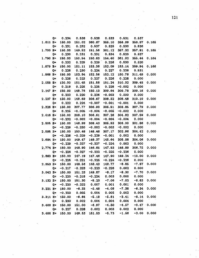
Q= 0 .234 0.538 0.528 0.533 0.531 0.5371.611 H= 150.00 151.02 360.67 355.10 356.99 359.97 0 .165

Q= 0.231 0.232 0.537 0.525 0 .530 0.5261.700 H= 150.00 149.52 151.56 361.12 357.32 357.81 0 .165

Q= 0.230 0.231 0.231 0.534 0.520 0.5271.790 H= 150.00 150.54 150.63 154.40 361.92 355.44 0 .164

q= 0.232 0.229 0.229 0.226 0 .530 0.5201.879 H= 150.00 151.11 153.38 152.09 153.14 359.94 0.166

q= 0.228 0.230 0.224 0.227 0.228 0.5311.968 H= 150.00 152.84 152.56 152.12 150.76 311.49 0.000

q= 0.228 0.223 0.227 0.226 0.228 0.0002.058 H= 150.00 151.45 151.58 151.24 310.32 309.45 0 .000

q= 0.219 0.225 0.225 0.228 -0 .0 0 2 0.0002.147 H= 150.00 148.76 150.13 309.64 309.78 309.16 0.000

q= 0.223 0.220 0.226 -0 .0 0 3 0.000 0.0002.237 H= 150.00 148.69 306.67 308.52 308.48 310.10 0 .000

q= 0.222 0.224 -0 .0 0 7 -0 .0 01 -0 .0 01 0.0002.326 H= 150.00 307.77 306.93 305.51 308.85 307.79 0 .000

q= 0.225 -0 .0 0 5 -0 .0 0 4 -0 .0 0 5 -0 .0 0 2 0.0002.416 H= 150.00 308.10 306.61 307.26 304.82 307.59 0 .000

q= -0 .2 3 2 -0 .0 0 2 -0 .0 0 4 -0 .0 0 4 -0 .0 0 4 0.0002.505 H= 150.00 148.99 308.43 305.93 306.00 301.86 0 .000

q= -0 .2 2 9 -0 .2 3 0 -0 .0 0 2 -0 .0 0 3 -0 .0 0 2 0.0002.595 H= 150.00 150.48 148.46 307.17 302.96 304.42 0 .0 0 0

q= -0 .2 2 8 -0 .2 2 9 -0 .2 29 -0 .0 01 0.002 0.0002.684 H= 150.00 149.47 149.37 145.64 305.58 304.06 0 .000

q= -0 .2 2 9 -0 .2 2 7 -0 .2 2 7 -0 .2 2 4 0 .002 0.0002.774 H= 150.00 148.90 146.65 147.93 146.89 306.75 0 .000

q= -0 .2 2 6 -0 .2 2 7 -0 .2 2 2 -0 .2 2 5 -0 .2 2 6 0.0002.863 H= 150.00 147.19 147.46 147.90 149.24 -1 0 .0 0 0 .000

q= -0 .2 2 5 -0 .2 21 -0 .2 2 5 -0 .2 2 4 -0 .2 2 6 0.0002.953 H= 150.00 148.56 148.43 148.77 -8 .8 5 -7 .9 7 0.000

q= -0 .2 1 7 -0 .2 2 3 -0 .2 2 3 -0 .2 2 6 0.002 0.0003.042 H= 150.00 151.23 149.87 -8 .1 7 -8 .3 0 -7 .7 0 0 .000

q= -0 .2 2 0 -0 .2 1 8 -0 .2 2 4 0.003 0.000 0.0003.132 H= 150.00 151.30 -5 .2 3 -7 .0 6 - 7 .0 2 -8 .6 3 0.000

q= -0 .2 2 0 -0 .2 2 2 0.007 0.001 0.001 0.0003.221 H= 150.00 -6 .3 3 -5 .4 8 -4 .0 8 -7 .3 8 -6 .3 4 0.000

q= -0 .2 2 3 0.005 0.004 0.005 0.002 0.0003.311 H= 150.00 -6 .6 4 -5 .1 8 -5 .8 1 -3 .4 1 -6 .1 4 0.000

q= 0.230 0.002 0.004 0,004 0.004 0.0003.400 E= 150.00 151.00 -6 .9 7 -4 .5 0 -4 .5 7 -0 .4 7 0.000

q= 0.227 0.228 0.002 0.003 0.002 0.0003.490 H= 150.00 149.53 151.53 -5 .7 3 -1 .5 6 -3 .0 0 0 .000

122

Q= 0.226 0.227 0.227 0.001 -0 .0 0 2 0.0003.579 H= 150.00 150.53 150.62 154.32 -4 .1 5 -2 .6 6 0 .000

Q= 0.227 0.225 0.225 0.222 -0 .0 0 2 0.0003.669 H= 150.00 151.09 153.32 152.05 153.08 -5 .3 1 0 .000

Q= 0.224 0.225 0.220 0.223 0 .224 0.0003.758 H= 150.00 152.78 152.52 152.09 150.75 308.54 0.000

Q= 0.223 0.219 0.223 0.222 0 .224 0.0003.848 H= 150.00 151.42 151.56 151.22 307.40 306.52 0.000

Q= 0.215 0.221 0.221 0.224 -0 .0 0 2 0.0003 .93 H= 150.00 148.78 150.13 306.73 306.85 306.26 0 .000

Q=, 0.218 0.216 0.222 -0 .0 0 3 0.000 0.0004.026 H= 150.00 148.71 303.82 305.62 305.59 307.17 0.000

Q= 0.218 0.220 -0 .0 0 7 -0 .0 01 -0 .0 01 0.0004.116 H= 150.00 304.91 304.06 302.68 305.94 304.92 0.000

Q= 0.221 -0 .0 0 5 -0 .0 0 4 -0 .0 0 5 -0 .0 0 2 0.0004.205 H= 150.00 305.21 303.77 304.39 302.01 304.71 0 .000

Q= -0 .2 2 8 -0 .0 0 2 -0 .0 0 4 -0 .0 0 4 -0 .0 0 4 0.0004.295 H= 150.00 149.01 305.54 303.10 303.16 299.10 0.000

Q= -0 .2 2 5 -0 .2 2 6 -0 .0 0 2 -0 .0 0 3 -0 .0 0 2 0.0004 .384 H= 150.00 150.47 148.49 304.31 300.19 301.60 0.000

Q= -0 .2 2 4 -0 .2 2 5 -0 .2 25 -0 .0 01 0.002 0.0004 .474 H= 150.00 149.48 149.38 145.72 302.75 301.28 0 .000

Q= -0 .2 2 5 -0 .2 2 3 -0 .2 23 -0 .2 2 0 0.002 0.000

123

REFERENCES

1. Azoury, P.H., Bassiri, A. M. and Najm, H., " Effect of Valve-Closure Schedule onWaterhammer," ASCE, Journal of Hydraulic Engineering, Vol. 112, No. 10, October 1986.

2 . Chaudhry, M. H., Applied Hydraulic Transients. Van Nostrand Reinhold Co., NewYork, 1979.

3 . Contractor, D. N., "Two and Three Stage Valve-Closures to MinimizeWaterhammer Transients." ASME, Vol. 98-7, 1985.

4 . Contractor, D. N., " Valve Stroking to Control Waterhammer Transient usingDynamic Programming," ASME Symp. Num. Methods in Fluid Transient Anal.,Fluids Engineering Division, Houston Texas, Jun. 1983.

5 . Conway, A. B., "Minimizing Waterhammer Transients in a Series Pipeline," M.S.thesis, Department of Civil Engineering and Engineering Mechanics, University of Arizona, 1986.

6 . Oriels, M. R., " Predicting Optimum Two-Stage Valve Closure," ASME, WinterAnnual Meeting, Houston, Texas, Nov. 1975. WA-75/FE-2.

7 . El-Ansary, A. S. and Contractor, D. N,,"Minimization of Axial Stresses andPressure Surges in Pipes using Nonlinear Optimization," ASME Vol. 140, Pressure Vessels and Piping Conference Pittsburgh,Pennsylvania, Jun. 1988.

8. Forsythe, G. E., Malcolm, M. A. and Moler, C. B., Computer Methods forMathematical Computations. Prentice-Hall, Inc., 1977.

9 . Goldberg, D. E. and Kerr, C. L , "Quick Stroking: Design of Time-Optimal ValveMotions," ASCE, Journal of Hydraulic Engineering, Vol. 113, No. 6, June 1 9 8 7 .

10 . Hornbeck, R. W „ Numerical Methods. Quantum Publishers^ Inc., 1975.

11 . Kuester, J. L. and Mize, J. H., Optimization Techniques with Fortran.McGraw-Hill, New York, 1973.

12 . Murray, W., Numerical Methods for Unconstrained Optimization. Academic PressInc., 1972.

124

13 . Nelder, J. A. and Mead, R , ° A Simplex Method for Function Minimization,"Computer Journal, Vol. 7, No. 4, 1965.

14 . Sen, S. and Contractor, D. N., "Reduction of Pressure Surges by MinimaxOptimization," Jour, of Applied Mathematics Modeling, Vol. 10, No. 4, August, 1986.

15 . Spendley, W., Next, G. R. and Himswort, F. R., " Sequential Application ofSimplex Design in Optimization and Evolutionary Design," Technometrics, Vol. 4, No. 4, 1962.

1 6 Streeter, V. L , " Valve Stroking to Control Water Hammer," Journal of the Hydraulics Division, ASCE, Vol. 89, No. HY2, Proc. Paper 3452, March 1963.

17. Streeter, V. L. and Wylie, E. B., Fluid Mechanics. McGraw-Hill, Inc., 1979.

18 . Watters. G. Z . . Analysis and Control of Unsteady Flow in Pipelines. ButterworthPublishers, 1984.

19 . Wiely, E. B., and Streeter, V. L , Fluid Transients. McGraw-Hill Inc., 1978.

optimal control of a valve to avoid column...

Documents