optimal control of a diesel engine with vgt and egr · optimal control of a diesel engine with vgt...

Optimal control of a diesel engine with VGTand EGR

Master’s thesisperformed in Vehicular Systems

byJonas Olsson and Markus Welander

Reg nr: LiTH-ISY-EX-44/3799-SE-2006

June 19, 2006

Optimal control of a diesel engine with VGTand EGR

Master’s thesis

performed in Vehicular Systems,Dept. of Electrical Engineering

at Linkopings universitet

by Jonas Olsson and Markus Welander

Reg nr: LiTH-ISY-EX-44/3799-SE-2006

Supervisor: Johan Wahlstrom

Examiner: Associate Professor Lars ErikssonLinkopings Universitet

Linkoping, June 19, 2006

AbstractTo fulfill todays requirements on emissions from engines, SCANIA has de-veloped an engine with EGR (Exhaust Gas Recirculation) and VGT (VariableGeometry Turbine). This gives two extra control signals to take into con-sideration. Open loop optimal control is used to investigate how these twoactuators should be controlled to minimize emissions and fuel consumption.A cost function, consisting of the errors between the most important variablesand their set points, has been used in the minimization. The variables are thetorque, the EGR mass fraction, the oxygen/fuel ratio and the pumping losses.From studies of the two control signals in different transients in the engine,information of how to control the VGT and EGR in the optimal way is found.The result from the optimal control has been compared with a PID simulationand has showed a better way to control the signals. The mayor reason whythe optimal control is better than a PID controller is the ability to use futurevalues from the transients.

Keywords: TOMOC, MATLAB, PID-controller, fmincon

iii

PrefaceThis master’s thesis has been performed at Vehicular System at LinkopingUniversity from September 2005 to May 2006, and is a part of PhD studentJohan Wahlstroms research.

AcknowledgmentWe would like to thank our supervisor Johan Wahlstrom and our examinerLars Eriksson for helping and supporting us. We also would like to thankAdam Lagerberg for helping us to use and understand TOMOC. A number offriends also deserves to be thanked for their help and support.

iv

Contents

Abstract iii

Preface and Acknowledgment iv

1 Introduction 11.1 Background . . . . . . . . . . . . . . . . . . . . . . . . . . 1

1.1.1 EGR . . . . . . . . . . . . . . . . . . . . . . . . . 11.1.2 VGT . . . . . . . . . . . . . . . . . . . . . . . . . 11.1.3 Objectives . . . . . . . . . . . . . . . . . . . . . . . 11.1.4 Earlier Work . . . . . . . . . . . . . . . . . . . . . 2

2 Engine Model 32.1 The model . . . . . . . . . . . . . . . . . . . . . . . . . . . 32.2 Engine dynamics . . . . . . . . . . . . . . . . . . . . . . . 5

2.2.1 Manifolds . . . . . . . . . . . . . . . . . . . . . . . 52.2.2 Turbo . . . . . . . . . . . . . . . . . . . . . . . . . 72.2.3 Stoichiometry combustion . . . . . . . . . . . . . . 72.2.4 Mass fraction in EGR, xegr . . . . . . . . . . . . . 8

2.3 Actuator dynamics . . . . . . . . . . . . . . . . . . . . . . 92.3.1 The EGR valve state . . . . . . . . . . . . . . . . . 92.3.2 The VGT position state . . . . . . . . . . . . . . . . 92.3.3 Fuel injection . . . . . . . . . . . . . . . . . . . . . 9

2.4 Summary . . . . . . . . . . . . . . . . . . . . . . . . . . . 9

3 Optimization and PID-regulation 103.1 Control objectives . . . . . . . . . . . . . . . . . . . . . . . 10

3.1.1 Cost function . . . . . . . . . . . . . . . . . . . . . 103.1.2 Constraints . . . . . . . . . . . . . . . . . . . . . . 12

3.2 ETC-Cycle . . . . . . . . . . . . . . . . . . . . . . . . . . 123.3 PID-regulation . . . . . . . . . . . . . . . . . . . . . . . . 133.4 Summary . . . . . . . . . . . . . . . . . . . . . . . . . . . 14

v

4 TOMOC 154.1 Introduction . . . . . . . . . . . . . . . . . . . . . . . . . . 15

4.1.1 Background . . . . . . . . . . . . . . . . . . . . . . 154.1.2 Function . . . . . . . . . . . . . . . . . . . . . . . 154.1.3 fmincon . . . . . . . . . . . . . . . . . . . . . . . . 17

4.2 Implementation . . . . . . . . . . . . . . . . . . . . . . . . 174.2.1 Implementation of the engine model in TOMOC . . 18

4.3 Summary . . . . . . . . . . . . . . . . . . . . . . . . . . . 19

5 Results 215.1 Simulations . . . . . . . . . . . . . . . . . . . . . . . . . . 21

5.1.1 Initial values . . . . . . . . . . . . . . . . . . . . . 215.1.2 ETC cycle . . . . . . . . . . . . . . . . . . . . . . . 225.1.3 EGR and VGT . . . . . . . . . . . . . . . . . . . . 225.1.4 Mass fraction in EGR . . . . . . . . . . . . . . . . . 225.1.5 Turbine speed . . . . . . . . . . . . . . . . . . . . . 255.1.6 Oxygen fraction in intake and exhaust manifold . . . 265.1.7 Oxygen to fuel ratio, λ . . . . . . . . . . . . . . . . 265.1.8 Torque . . . . . . . . . . . . . . . . . . . . . . . . 265.1.9 Intake- and exhaust manifold pressure . . . . . . . . 285.1.10 Time mean value . . . . . . . . . . . . . . . . . . . 28

5.2 Result with different weight parameters . . . . . . . . . . . 295.2.1 Low weight on xegr . . . . . . . . . . . . . . . . . 295.2.2 Low weight on λ . . . . . . . . . . . . . . . . . . . 335.2.3 Low weight on uδ . . . . . . . . . . . . . . . . . . 33

5.3 Turbine efficiency . . . . . . . . . . . . . . . . . . . . . . . 405.4 Compressor efficiency . . . . . . . . . . . . . . . . . . . . 445.5 Summary . . . . . . . . . . . . . . . . . . . . . . . . . . . 46

6 Conclusions 476.1 Cost function . . . . . . . . . . . . . . . . . . . . . . . . . 476.2 Results . . . . . . . . . . . . . . . . . . . . . . . . . . . . . 476.3 Control signals . . . . . . . . . . . . . . . . . . . . . . . . 48

6.3.1 Is this the optimal control? . . . . . . . . . . . . . . 486.4 Simulations . . . . . . . . . . . . . . . . . . . . . . . . . . 48

7 Future Work 497.1 Optimization . . . . . . . . . . . . . . . . . . . . . . . . . 49

References 50

Notation 51

vi

A TOMOC Manual 52A.1 Introduction . . . . . . . . . . . . . . . . . . . . . . . . . . 52A.2 Tomlkpg1start . . . . . . . . . . . . . . . . . . . . . . . . . 52

A.2.1 Phases . . . . . . . . . . . . . . . . . . . . . . . . . 53A.2.2 States . . . . . . . . . . . . . . . . . . . . . . . . . 53A.2.3 Control signals . . . . . . . . . . . . . . . . . . . . 53A.2.4 Initial values . . . . . . . . . . . . . . . . . . . . . 53A.2.5 Time constraints . . . . . . . . . . . . . . . . . . . 53A.2.6 Initial guesses . . . . . . . . . . . . . . . . . . . . . 54

A.3 tomlkpg1fun . . . . . . . . . . . . . . . . . . . . . . . . . . 55A.4 tomlkpg1dynfun . . . . . . . . . . . . . . . . . . . . . . . . 56A.5 tomlkpg1initpar . . . . . . . . . . . . . . . . . . . . . . . . 57A.6 tomlkpg1constraints . . . . . . . . . . . . . . . . . . . . . . 57A.7 tomocinitguess . . . . . . . . . . . . . . . . . . . . . . . . 57A.8 tomocconph . . . . . . . . . . . . . . . . . . . . . . . . . . 58A.9 tomoccon . . . . . . . . . . . . . . . . . . . . . . . . . . . 58A.10 tomocpostproc . . . . . . . . . . . . . . . . . . . . . . . . . 58

vii

Chapter 1

Introduction

1.1 Background

1.1.1 EGRHigher and higher environmental requirements are demanded from todays en-gines which means that the industry constantly have to develop new methodsto reduce emissions. One method the engine industry have come up with tolower the emissions is called EGR (Exhaust Gas Recirculation), which meansthat some of the exhaust gas is recycled back into the engine to cool down thecombustion temperature which leads to reduced NOx emissions.

1.1.2 VGTVGT (Variable Geometry Turbine) is a variable restriction which controlshow much exhaust gas that is lead in to the turbo. The VGT has a set ofvanes which can be used to control the turbine inlet pressure. The closing ofthe VGT vanes leads to an increase in the turbine inlet pressure which makesthe turbine to spin faster and generate more boost in the engine. The VGT isalso used to build up the needed pressure in the exhaust manifold in order torecirculate the exhaust gases back to the engine.

1.1.3 ObjectivesThe objective with this master’s thesis is to find the optimal way to controlthe VGT and EGR in order to lower the emissions from the engine. Earlier aPID controller has been used to control the two valves, but since the systemof the engine is non linear and cross correlated it is very difficult to see if aPID controller gives the best possible control. Since optimal control can not

1

2 Introduction

be used in the reality to control the two valves, it is used as a comparison forother control methods.

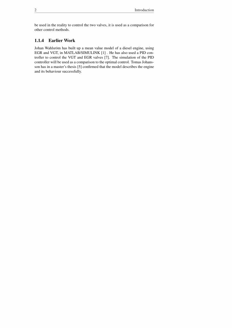
1.1.4 Earlier WorkJohan Wahlsrom has built up a mean value model of a diesel engine, usingEGR and VGT, in MATLAB/SIMULINK [1] . He has also used a PID con-troller to control the VGT and EGR valves [7]. The simulation of the PIDcontroller will be used as a comparison to the optimal control. Tomas Johans-son has in a master’s thesis [5] confirmed that the model describes the engineand its behaviour successfully.

Chapter 2

Engine Model

In this chapter the dynamic of the engine and it’s functions will be explained.The equations of the states, control signals and some of the most importantcontrol parameters will be described.

2.1 The model

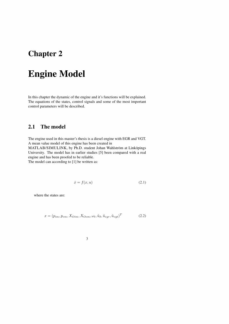
The engine used in this master’s thesis is a diesel engine with EGR and VGT.A mean value model of this engine has been created inMATLAB/SIMULINK, by Ph.D. student Johan Wahlstrom at LinkopingsUniversity. The model has in earlier studies [5] been compared with a realengine and has been proofed to be reliable.The model can according to [1] be written as:

x = f(x, u) (2.1)

where the states are:

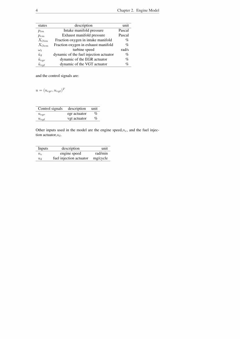
x = (pim, pem, XOim, XOem, ωt, uδ, uegr, uvgt)T (2.2)

3

4 Chapter 2. Engine Model

states description unitpim Intake manifold pressure Pascalpem Exhaust manifold pressure PascalXOim Fraction oxygen in intake manifold %XOem Fraction oxygen in exhaust manifold %ωt turbine speed rad/suδ dynamic of the fuel injection actuator %uegr dynamic of the EGR actuator %uvgt dynamic of the VGT actuator %

and the control signals are:

u = (uegr, uvgt)T

Control signals description unituegr egr actuator %uvgt vgt actuator %

Other inputs used in the model are the engine speed,ne, and the fuel injec-tion actuator,uδ .

Inputs description unitne engine speed rad/minuδ fuel injection actuator mg/cycle

2.2. Engine dynamics 5

EGR cooler

Exhaustmanifold

CompressorIntercooler

Cylinders

Turbine

EGR valve

Intakemanifold

Wegr

Wei Weo pem

XOemXOim

pim

nt

uδ

Wt

Wc

uvgt

uegr

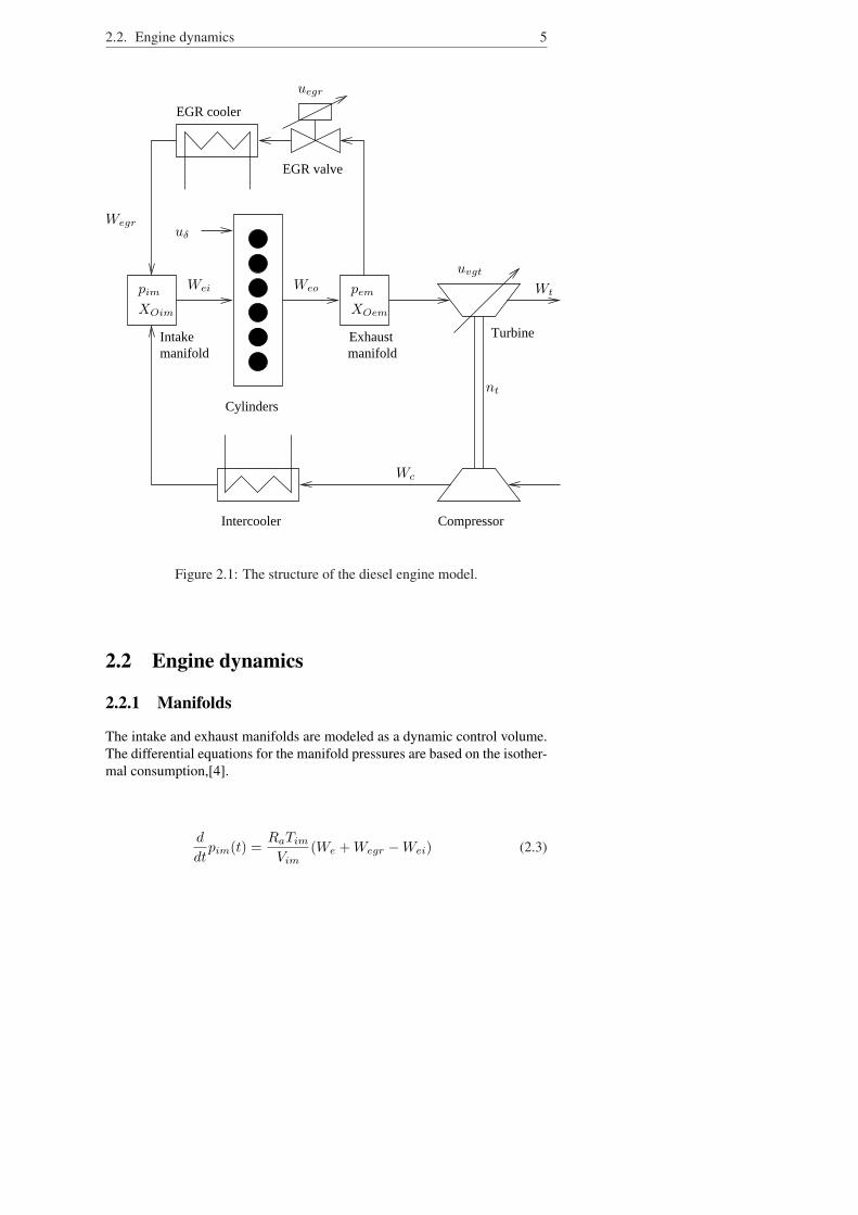
Figure 2.1: The structure of the diesel engine model.

2.2 Engine dynamics

2.2.1 Manifolds

The intake and exhaust manifolds are modeled as a dynamic control volume.The differential equations for the manifold pressures are based on the isother-mal consumption,[4].

d

dtpim(t) =

RaTim

Vim(We + Wegr −Wei) (2.3)


d

dtpem(t) =

ReTem

Vem(Weo + Wt −Wegr) (2.4)

The EGR fraction in the intake manifold is based on the inflow.

xegr =Wegr

Wc + Wegr(2.5)

The dynamic of XOim(oxygen concentration in intake manifold) and XOem

(Oxygen fraction in exhaust manifold) can be derived as [6]:

d

dtXOim(t) =

RaTim

pimVim(Wegr(XOem −XOim) + Wc(XOc −XOim)) (2.6)

d

dtXOem(t) =

ReTem

pemVem(Weo(XOe −XOem)) (2.7)

where XOc is the oxygen concentration of the gas flow past the compres-sor i.e. the same as in air, and XOe the oxygen concentration in the exhaustgases out from the engine cylinders.

Symbol Description unitW Flow g/sT Temperature KRa Gas constant for air J/(kg ·K)Re Gas constant for exhaust gas J/(kg ·K)V Volume m3

2.2. Engine dynamics 7

2.2.2 TurboThe turbo speed is modeled using a dynamic system with an inertia Jt

d

dtωt(t) =

Mt −Mc

Jt(2.8)

Mt is the driving torque from the turbine and Mc is the braking torque fromthe compressor.

2.2.3 Stoichiometry combustionIn a diesel engine it is very important to keep control on the air/fuel ratio(A/F ) = ma

mfin order to decrease the smoke emission. A stoichiometric

combustion reaction between a general hydrocarbon fuel and air, where therest product only consists of water and carbon monoxide looks like

CaHb + (a + b4 )(O2 + 3.773N2) → aCO2 + b

2H2O + 3.773(a + b4 )N2

(2.9)

Where a and b represent the number of carbon and hydrogen atoms in onemolecule in the fuel that are used in the engine. What is interesting in thisequation is the relation between a and b, y = a

b which shows the relativeamount carbon in the fuel. It is now possible, using the molecular weights forcarbon, hydrogen, oxygen and nitrogen, to write an expression for the stoi-chiometric mixture.

(A/F )s = ma

mf s= (1+y/4)(32+3.773·28.16)

12.011+1.1008y = 34.56(4+y)12.011+1.008y

(2.10)

(A/F )s has usually a value around 14.3.

We can now define λ , the air/fuel equivalence ratio, as:


λ =(A/F )(A/F )s

(2.11)

If λ > 1 it is indicate a surplus of air and if λ < 1 it’s indicate a surplus offuel. In a diesel engine λ must be larger than a minimum limit, e.g to avoidto much smoke emission.

Since it’s the oxygen fraction and not the air fraction that is used in the model,λ is modeled as:

λ =WeiXOim

WfOc(A/F )s(2.12)

Symbol Description unitWei Air flow in intake manifold g/sWf Fuel flow g/sOc Fraction oxygen in air %

2.2.4 Mass fraction in EGR, xegr

Introducing exhaust gases in the air-fuel mixture will reduce the combustiontemperature and thereby reduce NOx gases. Both emissions and fuel con-sumption will decrease with raised EGR ratio. xegr is the mass fraction ofexhaust gases in the air-fuel mixture. If xegr is to low there will be to muchNOx emissions and if it is to high there will be to much smoke. The EGRfraction also displaces fresh oxygen, making it less available for combustionand thus reducing the probability of interaction between nitrogen and oxygenatoms even under lean conditions.

Emission limits are formulated as set-points in EGR fraction. It is thereforedesirable to minimize the error between the xegr mass fraction and it is setpoint, in a optimization point of view.

Opening the EGR valve will reduce the exhaust manifold pressure and therebyreduce the turbine speed. Opening the VGT valve will reduce exhaust mani-fold pressure and also decrease EGR fraction.

2.3. Actuator dynamics 9

2.3 Actuator dynamics

2.3.1 The EGR valve stateuegr describes the EGR actuator dynamic and can be derived as:

d

dtuegr =

1τegr

(uegr − uegr) (2.13)

The EGR throttle is open when uegr=100% and closed when uegr=0%

2.3.2 The VGT position stateuvgt describes the VGT actuator dynamic and can be derived as:

d

dtuvgt =

1τvgt

(uvgt − uvgt) (2.14)

The VGT position is open when uvgt=100% and closed when uvgt=0%

2.3.3 Fuel injectionThe amount of fuel injected udelta can be derived as

d

dtudelta =

1τdelta

(udelta − udelta) (2.15)

which describes the actuator dynamic.

2.4 SummaryAll the necessary equations and constants that are needed to describe the dy-namic of the engine are available. The states and control signals are alsosuccessfully described.

Chapter 3

Optimization andPID-regulation

This chapter describes the optimization parameters, the control objectives andthe cost function. The ETC cycle and the PID structure will also be described.

3.1 Control objectivesTo fulfill all necessary requirements, the engine has to have a number of con-trol goals. When values are received from the ETC-cycle it is important toknow which parameters to control. In this case the control goals are:

1. Follow the set-point engine torque from the ETC-cycle.

2. Minimize the error between the xegr fraction and its set point. If xegr

is to low there will be to much NOx emissions and if it is to high therewill be to much smoke.

3. In order to decrease the smoke, λ is not allowed to go below a certainlimit.

4. The turbine speed, ωt, can not be allowed to exceed a maximum limit,otherwise the turbo charger can be damaged.

5. Minimize pump losses in order to decrease the fuel consumption.

3.1.1 Cost functionThe cost function is designed to take into consideration a number of differentphysical functions in the engine. It is also gives the possibility to weight dif-

10

3.1. Control objectives 11

ferent functions more than others.

The cost function used in this master’s thesis is

min

n∑

j=1

C1(uδsetp(j)− uδ(j))2 + C2(xegr(j)− xegrSetp(j))2+ (3.1)

C3(pem(j)− pim(j)) + C4(max(λSetp(j)− λ(j), 0))2+

C5(uegr(j)− uegr(j − 1))2 + C6(uvgt(j)− uvgt(j − 1))2

The first term minimizes the quadratic error between the real fuel injection(uδ) and the desired fuel injection (uδsetp), which is calculated from the ETCcycle by the following equation.

uδsetp = k1ne(t)2 + k2ne(t) + k3MeSetp(t) + k4(Pem − Pim) + k5 (3.2)

where MeSetp(t) is the torque, ne is the engine speed and k1, k2, k3, k4, k5

are constants.

The second term is the quadratic error between EGR fraction (xegr) and thereference value xegrSetp. In this case xegrSetp has been set to 0.15, that is avalue which was obtained from stationary measurements with emissions justbelow the legislated requirements(see [7]). This term helps control objective2 in section 3.1 to be fulfilled.

The third term is the pump loses, which is the difference between the intakeand exhaust manifold pressures. The reason to not minimize the quadraticerror in the pumping loses is that a negative value is possible to attain, whichis an advantage when minimizing the fuel consumption but a disadvantagewhen minimizing the xegr. This term helps to fulfill control objective 5 insection 3.1.

The fourth term minimizes the difference between λ and λSetp. λSetp hasbeen obtained in the same way as xegrSetp. In this case xegrSetp is 1.8. Sincethere is no negative with a high λ, the whole term is set to zero if λ is higherthan 1.8. This helps control objective 3 in section 3.1 to be fulfilled.The fifth and sixth term is a way to avoid to much ripple in the control sig-nals. The control signal is compared with an earlier signal and the differencebetween them is minimized.C1, C2, C3,C4,C5 and C6 are parameters chosen depending on how much the

12 Chapter 3. Optimization and PID-regulation

different terms are weight to each other. These are set depending on whichterm in the cost function that is desired to have the most influence. How thedifferent terms effects the result will be described in section 5.

3.1.2 ConstraintsIn order to reach todays requirement on emissions, some limitations have tobe set. It is also necessary to limit some physical values. The constraints inthe optimization are

• λ ≥ 1.3 to prevent to much smoke emissions.

• nt ≤ 1.1 ∗ 105 rpm to make sure that the engine do not get damaged.nt is the turbine speed

• uδ ≥ 0 ,the fuel injection can not be negative.

• 0% ≤ uegr ≤ 100%

• 10% ≤ uvgt ≤ 100%

The states and control signals are also constrained in order to make the simu-lation time as short as possible. A higher number of constraints means fewernumber of possible solutions which means a shorter simulation time. Theconstraints have been chosen after what is realistic for an diesel engine of thiskind. There are also a number of constraints that have been set on physicalparameters to make sure that the model will work in a realistic way (for ex-ample temperature T can not be below 0 K), those constraints are the same asin the original simulink model.

3.2 ETC-CycleAs a reference for the following optimization the ETC-cycle (European Tran-sient Cycle) has been used. This cycle is used for emission certification ofheavy-duty diesel engines in Europe, starting in the year 2000. Differentdriving conditions are represented by three parts of the ETC cycle.

• Part 1 (0-600 s) represents city driving with a maximum speed of 50km/h, frequent starts, stops and idling.

3.3. PID-regulation 13

• Part 2 (600-1200 s) represents rural driving, starting with a steep accel-eration segment. The average speed is about 72 km/h.

• Part 3 (1200-1800 s) is motorway driving with average speed of about88 km/h.

Values from the ETC cycle comes in three parts. Vehicle Speed, Engine speedand Engine Torque as function of time. Where the sample time is one sec-ond. In this case the engine speed and torque has been used. In this case theengine speed from the ETC-cycle is the control signal ne. The signal is takendirectly from the cycle and is implemented in TOMOC as a simple bound.By setting the upper bound (UB) equal to the lower bound (LB) ne will betreated as a fixed value in the optimization. But since the sample time fromthe ETC-cycle is 1 sec this signal have to be interpolated to get a higher reso-lution. This is solved by using the interpolation command in MATLAB. Theresult is a vector from t1 to t2 with the desired sample time as length. Thedesired fuel injection is calculated with values from torque and engine speedfrom the ETC-cycle.

u = C1n2e + C2ne + C3Me + C4(Pem − Pim) + C5 (3.3)

This value is then a part of the cost function where the goal is to get the realfuel injection to follow the calculated one.

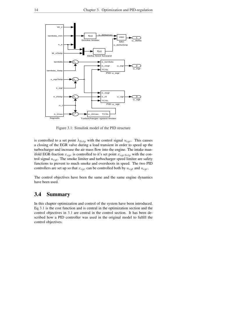
3.3 PID-regulationIn the original simulink model of the engine, a PID controller is used to reg-ulate the control signals. The design objective for the PID controller is tocoordinate uδ , uegr and uvgt in order to achieve the control objectives. Infigure 3.1 a simulink schematic of the control structure is shown. The signalsneeded for the controller are shown as signals in figure 3.1. The set pointsand limits for the controllers are obtained from stationary measurements withemissions just below the legislated requirements and represented as look uptables as a function of operation condition. In tuning these set points are heldconstant. The engine torque is controlled to it’s set point MeSetp with thecontrol signal udelta using feed forward. The block Delta feed forward infigure 3.1 calculates the set point value for udelta.

uδsetp = c1ne(t)2 + c2ne(t) + c3MeSetp(t) + c4(Pem − Pim) + c5

The parameters C1 to C4 are estimated from stationary measurements. λ

14 Chapter 3. Optimization and PID-regulation

3

u_vgt

2

u_egr

1

u_delta

e_ntmax TCSL

Turbocharger speed limiter

f(u)

Smoke limiter

W_c

lambda_min

n_e

M_eSetp

lambda

lambda_Setp

x_egrSetp

x_egr

n_tSetp

n_t

n_tmax

Signals

e_xegr

e_nt

TCSL

u_vgt

PID u_vgt

e_lambda

e_xegr

TCSL

u_egr

PID u_egr

min

Min

f(u)

Delta feed forward

u_deltamax

u_deltaSetp

Figure 3.1: Simulink model of the PID structure

is controlled to a set point λSetp with the control signal uegr. This causesa closing of the EGR valve during a load transient in order to speed up theturbocharger and increase the air mass flow into the engine. The intake man-ifold EGR-fraction xegr is controlled to it’s set point xegrSetp with the con-trol signal uvgt. The smoke limiter and turbocharger speed limiter are safetyfunctions to prevent to much smoke and overshoots in speed. The two PIDcontrollers are set up so that xegr can be controlled both by uvgt and uegr.

The control objectives have been the same and the same engine dynamicshave been used.

3.4 SummaryIn this chapter optimization and control of the system have been introduced.Eq 3.1 is the cost function and is central in the optimization section and thecontrol objectives in 3.1 are central in the control section. It has been de-scribed how a PID controller was used in the original model to fulfill thecontrol objectives.

Chapter 4

TOMOC

In this chapter the engine model and the optimization is put together and aoptimal control problem is formulated. The optimization algorithm TOMOCis described and explained.

4.1 Introduction

4.1.1 Background

TOMOC is an optimization algorithm developed by Adam Lagerberg at theSchool of Engineering Jonkopings University, in his PhD thesis. TOMOC isdescribed in [2]. TOMOC is used for solving optimal control problems. Thereexists many different methods to solve optimization problems and there aremany different software tools to use. But the usual optimization problem donot consider the dynamics, that are used in optimal control problems. TO-MOC reforms the optimal control problem into a numerical minimizationproblem which can be solved in MATLAB. TOMOC was originally designedto use the general NLP-solvers implemented in TOMLAB, but since TOM-LAB is not available in this thesis, a special version of TOMOC which usesthe MATLAB function fmincon which follows with the optimization tool-box has been used.

4.1.2 Function

A general optimal control problem can be formulated as followes [3].

Find the control function u(t), t ∈ [tI , tF ] that minimize the cost function.

15

16 Chapter 4. TOMOC

J = Φ(x(tI), x(tF ), tI , tF ) +∫ tF

tI

L(x(t), u(t), t)dt (4.1)

The first part of the function defines cost related to the final and initialstates. x(t) is a vector containing all the states and u(t) is a vector containingthe control signals.The state equations that defines the dynamic are:

x = f(x(t), u(t), t) (4.2)

u(t) ∈ U, 0 ≤ t ≤ tF (4.3)

x(0) = x0, Φ(x(tF )) = 0 (4.4)

Simple boundary conditions are:

x(tI) = xI (4.5)

x(tF ) = xF (4.6)

Complex boundary conditions are:

gI(x(tI), u(tI)) = 0 (4.7)

gF (x(tF ), uF ) = 0 (4.8)

Simple constraints on state and control variables are:

xmin ≤ x(t) ≤ xmax, t ∈ [tI , tF ] (4.9)

umin ≤ u(t) ≤ umax, t ∈ [tI , tF ] (4.10)

Complex path constraints are:

gL ≤ g(x(t), u(t), t) ≤ gU , t ∈ [tI , tF ] (4.11)

The final time, tF can be fixed or allowed to vary and be a part of the opti-mization problem.

The central idea in TOMOC is to implement a transcription formulation of the

4.2. Implementation 17

dynamics equation.The transcription is based on a direct collocation formulawhich discretizise the differential equations tons to solve the optimal controlproblem. The basis of this approach is a finite dimensional approximationof control and state variables i.e. a discretization. From this discretization, aconstrained optimal control problem is transformed into a finite dimensionalnonlinear program which can be solved by a standard NPL solvers. TOMOCtransforms the differential equation to a non linear problem, with methodssuch as Euler or Runge-kutta. The non linear problem can be written as:

J = Φ(x(tI), x(tF ), tI , tF ) +N∑

j=0

L(xj , uj) (4.12)

The non linear problem can be solved in MATLAB by fmincon.

4.1.3 fminconfmincon is a MATLAB function which solves non linear optimization prob-lems. fmincon uses a method called SQP (Sequential Quadratic Program-ming) to find a constrained minimum of a scalar function of several variablesstarting at an initial estimate. fmincon starts at X0 and attempts to find aminimum X to the function described in cost function subject to the linear in-equalities. In this case X0 is a vector. The function to be minimized, the costfunction, is a function that accepts a vector x and returns a scalar f. There isno way to know if the found minimum is local or global, because fminconalways searches locally for decreasing solutions.

4.2 ImplementationTo make fmincon work we need the following in data.

[X] =fmincon(FUN,X0,Aieq,Bieq,Aeq,Beq,LB,UB,NONLCON,OPTIONS,P)

(4.13)

where

• FUN is the cost function.

• X0 are the initial values.

18 Chapter 4. TOMOC

• Aeq and Beq are inequality constraints.

• Aeq and Beq are equality constraints.

• LB and UB are lower and upper bounds for the states and control sig-nals.

• NONLCON are the linear and nonlinear constraints.

• OPTIONS are parameters for the simulation.

P is a struct in MATLAB that contains user defined options.

With these values fmincon gives a vector X that contains values of thestates and control signals that minimize the cost function for a specific timeinterval.

In the original TOMOC, A and B are matrices that describes the dynamicon the form x = Ax + Bu. However, it is only possible to have the dynamicon this form if it is linear. In the diesel engine dynamic, that is not the case.Therefore it is necessary to get the dynamic from a separate file. The fileStatesmaker uses the engine dynamic and creates the wanted states, andreturn them on correct form to the start file and fmincon.

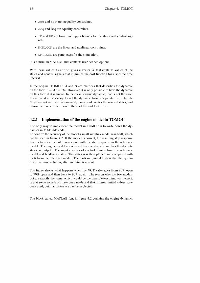
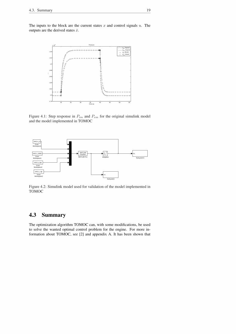
4.2.1 Implementation of the engine model in TOMOCThe only way to implement the model in TOMOC is to write down the dy-namics in MATLAB code.To confirm the accuracy of the model a small simulink model was built, whichcan be seen in figure 4.2. If the model is correct, the resulting step responsefrom a transient, should correspond with the step response in the referencemodel. The engine model is collected from workspace and has the derivatestates as output. The input consists of control signals from the referencemodel and feedback states. The states was then plotted and compared withplots from the reference model. The plots in figure 4.1 show that the systemgives the same solution, after an initial transient.

The figure shows what happens when the VGT valve goes from 90% opento 70% open and then back to 90% again. The reason why the two modelsnot are exactly the same, which would be the case if everything was correct,is that some rounds off have been made and that different initial values havebeen used, but that difference can be neglected.

The block called MATLAB fcn, in figure 4.2 contains the engine dynamic.

4.3. Summary 19

The inputs to the block are the current states x and control signals u. Theoutputs are the derived states x.

20 25 30 35 40 45 50 551.78

1.8

1.82

1.84

1.86

1.88

1.9

1.92

1.94

x 105

Pa

Time (s)

Pressure

p

im Orginal

pem

Orginal

pim

Model

pem

Model

Figure 4.1: Step response in Pim and Pem for the original simulink modeland the model implemented in TOMOC

In1

Subsystem1

In1

Subsystem

MATLABFunction

MATLAB Fcn

1s

Integrator

sim1.n_e

From Workspace4

sim1.u_egr

FromWorkspace3

sim1.u_vgt

FromWorkspace2

sim1.u_delta

FromWorkspace1

Figure 4.2: Simulink model used for validation of the model implemented inTOMOC

4.3 SummaryThe optimization algorithm TOMOC can, with some modifications, be usedto solve the wanted optimal control problem for the engine. For more in-formation about TOMOC, see [2] and appendix A. It has been shown that

20 Chapter 4. TOMOC

the model implemented in TOMOC is correct since it gives the same stepresponse as the original simulink model.

Chapter 5

Results

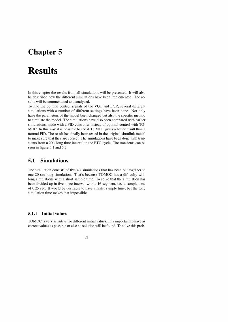
In this chapter the results from all simulations will be presented. It will alsobe described how the different simulations have been implemented. The re-sults will be commentated and analyzed.To find the optimal control signals of the VGT and EGR, several differentsimulations with a number of different settings have been done. Not onlyhave the parameters of the model been changed but also the specific methodto simulate the model. The simulations have also been compared with earliersimulations, made with a PID controller instead of optimal control with TO-MOC. In this way it is possible to see if TOMOC gives a better result than anormal PID. The result has finally been tested in the original simulink modelto make sure that they are correct. The simulations have been done with tran-sients from a 20 s long time interval in the ETC-cycle. The transients can beseen in figure 5.1 and 5.2

5.1 SimulationsThe simulation consists of five 4 s simulations that has been put together toone 20 sec long simulation. That’s because TOMOC has a difficulty withlong simulations with a short sample time. To solve that the simulation hasbeen divided up in five 4 sec interval with a 16 segment, i.e. a sample timeof 0.25 sec. It would be desirable to have a faster sample time, but the longsimulation time makes that impossible.

5.1.1 Initial values

TOMOC is very sensitive for different initial values. It is important to have ascorrect values as possible or else no solution will be found. To solve this prob-

21

22 Chapter 5. Results

390 392 394 396 398 400 402 404 406 408 4101200

1250

1300

1350

1400

1450

1500

1550

1600

ne ETC−cycle

Time (s)

rpm

Figure 5.1: The engine speed from the ETC cycle.

lem values from earlier simulations, with a PID regulator, have been used.This can only be done with the assumption that the PID regulator gives a re-sult that is rather close to the optimal result. This means that the result willhave the same principal appearance as the PID simulation, but since the reg-ulation objectives are the same, it is quite natural.

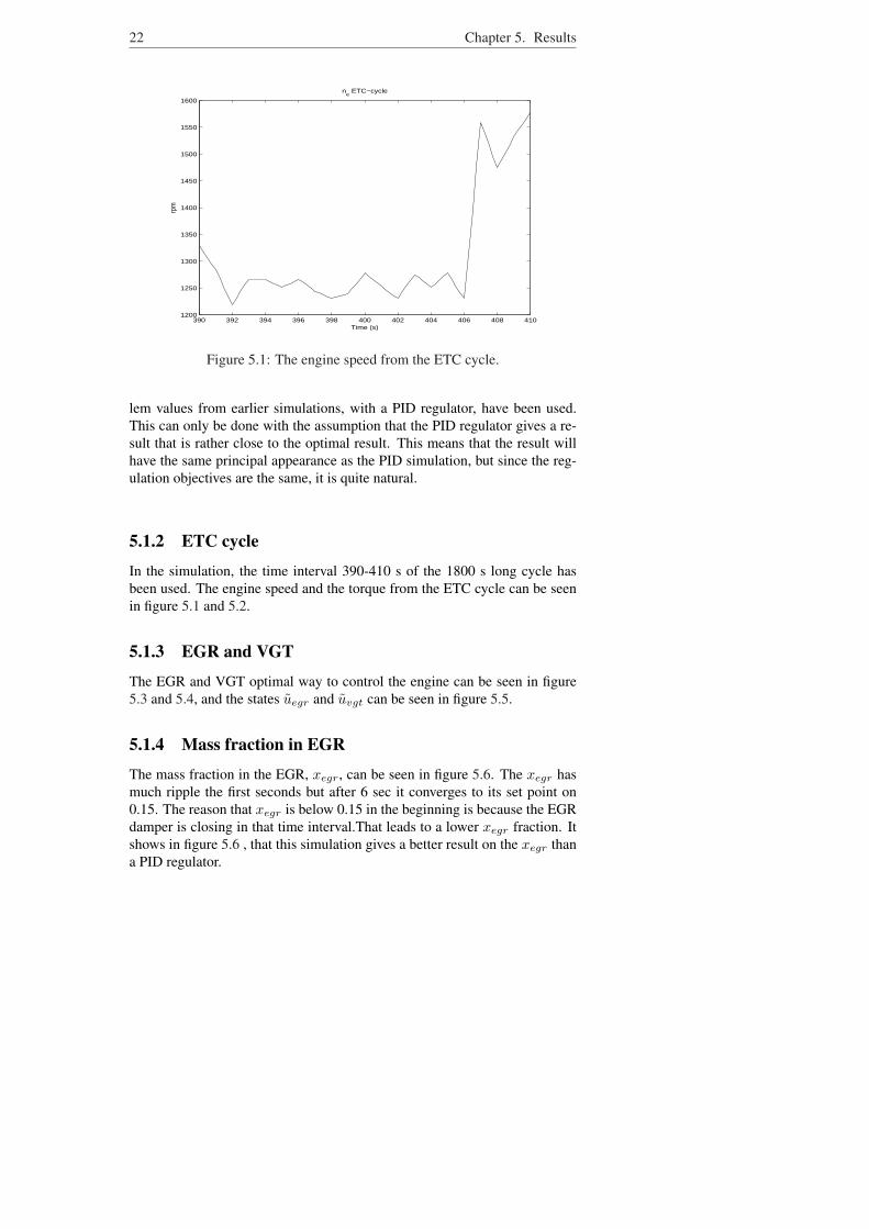
5.1.2 ETC cycle

In the simulation, the time interval 390-410 s of the 1800 s long cycle hasbeen used. The engine speed and the torque from the ETC cycle can be seenin figure 5.1 and 5.2.

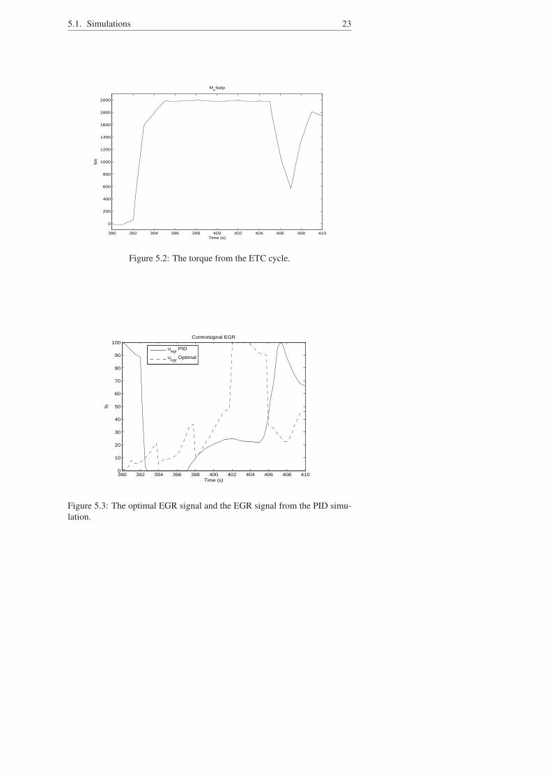
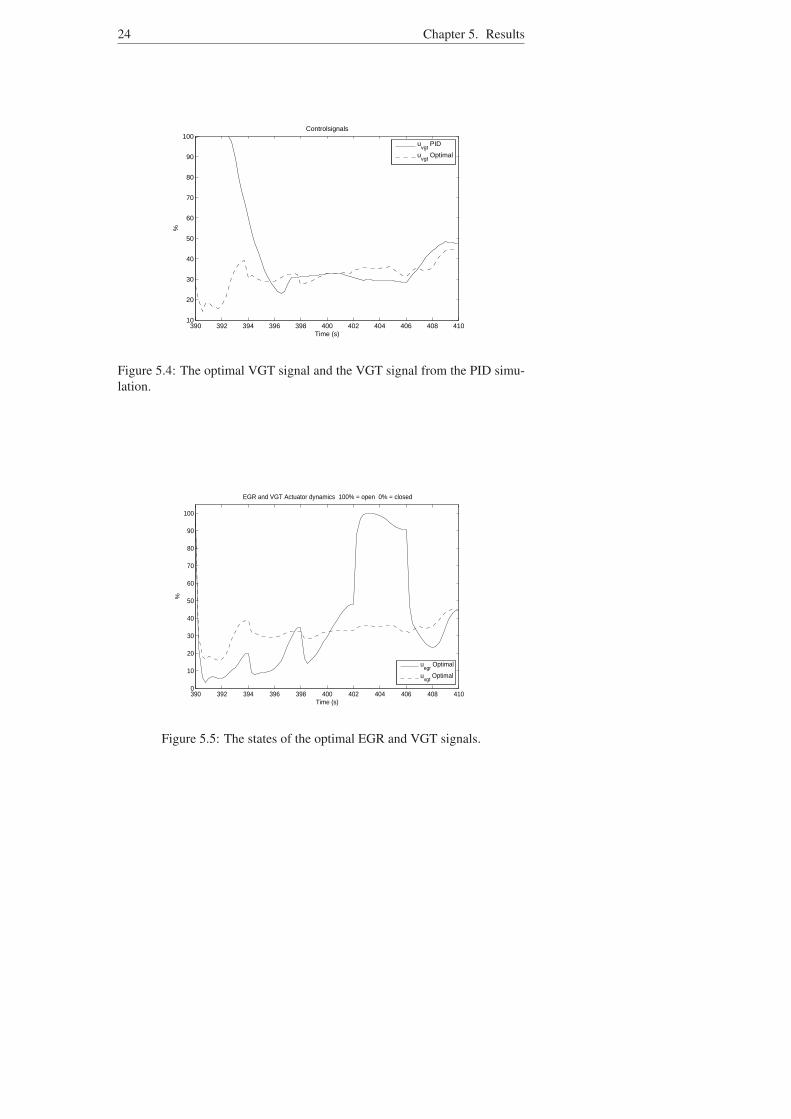
5.1.3 EGR and VGT

The EGR and VGT optimal way to control the engine can be seen in figure5.3 and 5.4, and the states uegr and uvgt can be seen in figure 5.5.

5.1.4 Mass fraction in EGR

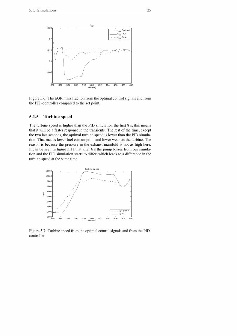
The mass fraction in the EGR, xegr, can be seen in figure 5.6. The xegr hasmuch ripple the first seconds but after 6 sec it converges to its set point on0.15. The reason that xegr is below 0.15 in the beginning is because the EGRdamper is closing in that time interval.That leads to a lower xegr fraction. Itshows in figure 5.6 , that this simulation gives a better result on the xegr thana PID regulator.

5.1. Simulations 23

390 392 394 396 398 400 402 404 406 408 410

0

200

400

600

800

1000

1200

1400

1600

1800

2000

Time (s)

Nm

MeSetp

Figure 5.2: The torque from the ETC cycle.

390 392 394 396 398 400 402 404 406 408 4100

10

20

30

40

50

60

70

80

90

100Controlsignal EGR

Time (s)

%

u

egr PID

uegr

Optimal

Figure 5.3: The optimal EGR signal and the EGR signal from the PID simu-lation.


390 392 394 396 398 400 402 404 406 408 41010

20

30

40

50

60

70

80

90

100Controlsignals

Time (s)

%

u

vgt PID

uvgt

Optimal

Figure 5.4: The optimal VGT signal and the VGT signal from the PID simu-lation.

390 392 394 396 398 400 402 404 406 408 4100

10

20

30

40

50

60

70

80

90

100

EGR and VGT Actuator dynamics 100% = open 0% = closed

Time (s)

%

uegr

Optimal

uvgt

Optimal

Figure 5.5: The states of the optimal EGR and VGT signals.

5.1. Simulations 25

390 392 394 396 398 400 402 404 406 408 4100

0.05

0.1

0.15

0.2

0.25

xegr

Time (s)

x

egr Optimal

xegr

PID

xegr

Setp

Figure 5.6: The EGR mass fraction from the optimal control signals and fromthe PID-controller compared to the set point.

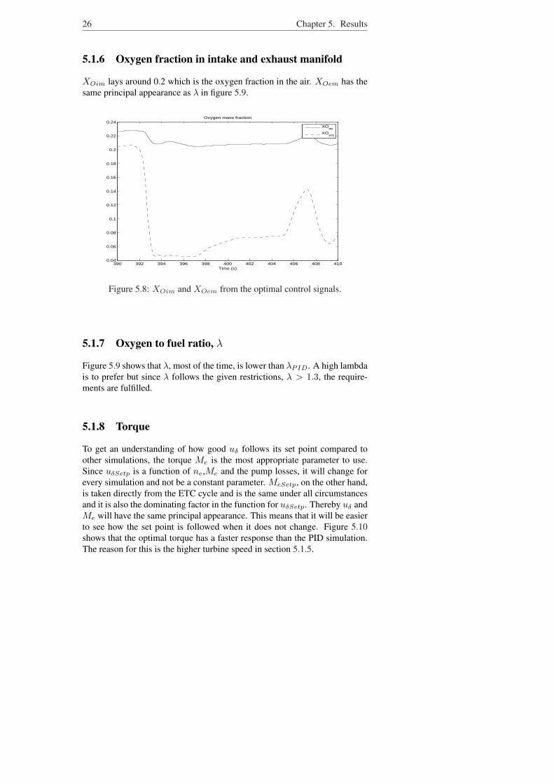
5.1.5 Turbine speed

The turbine speed is higher than the PID simulation the first 8 s, this meansthat it will be a faster response in the transients. The rest of the time, exceptthe two last seconds, the optimal turbine speed is lower than the PID simula-tion. That means lower fuel consumption and lower wear on the turbine. Thereason is because the pressure in the exhaust manifold is not as high here.It can be seen in figure 5.11 that after 6 s the pump losses from our simula-tion and the PID simulation starts to differ, which leads to a difference in theturbine speed at the same time.

390 392 394 396 398 400 402 404 406 408 4102000

3000

4000

5000

6000

7000

8000

9000

10000

11000Turbine speed

Time (s)

rad/

s

ωt Optimal

ωt PID

Figure 5.7: Turbine speed from the optimal control signals and from the PID-controller.


5.1.6 Oxygen fraction in intake and exhaust manifold

XOim lays around 0.2 which is the oxygen fraction in the air. XOem has thesame principal appearance as λ in figure 5.9.

390 392 394 396 398 400 402 404 406 408 4100.04

0.06

0.08

0.1

0.12

0.14

0.16

0.18

0.2

0.22

0.24Oxygen mass fraction

Time (s)

XO

im

XOem

Figure 5.8: XOim and XOem from the optimal control signals.

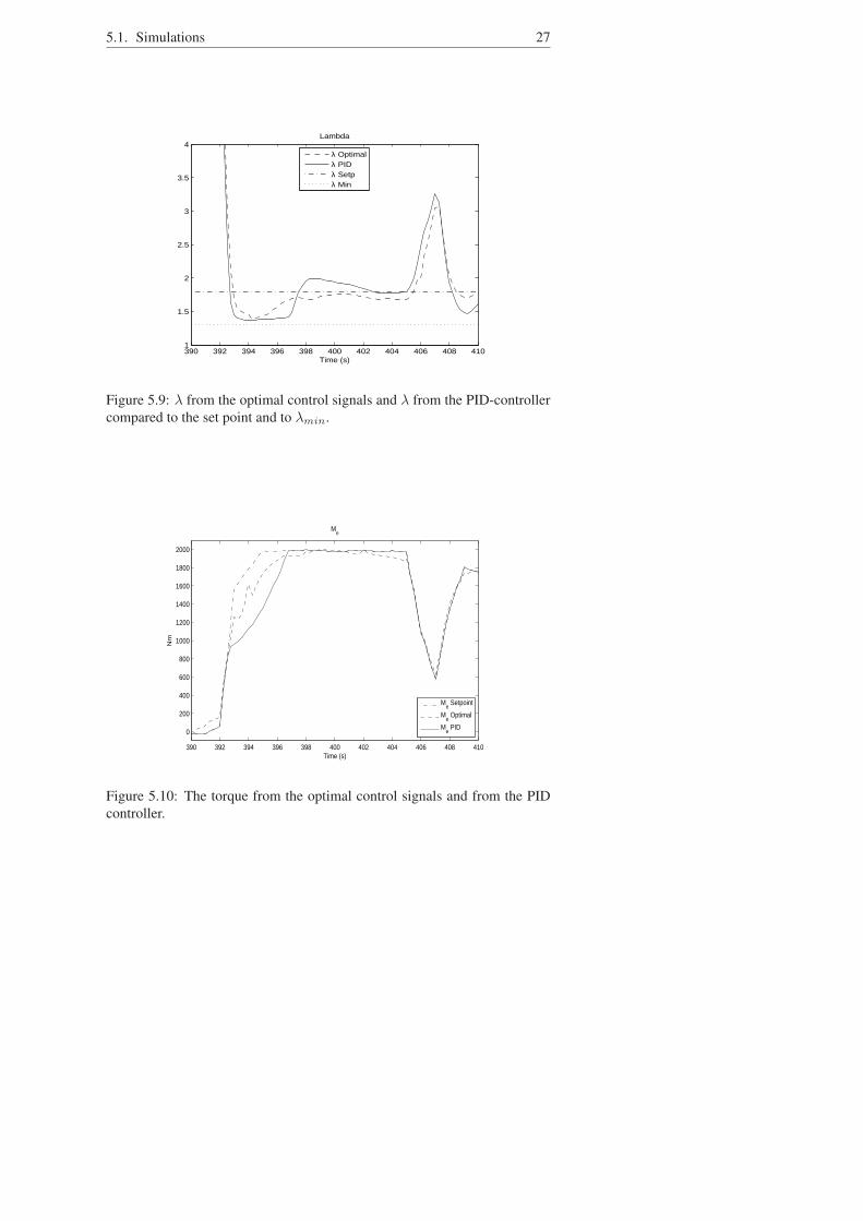
5.1.7 Oxygen to fuel ratio, λ

Figure 5.9 shows that λ, most of the time, is lower than λPID. A high lambdais to prefer but since λ follows the given restrictions, λ > 1.3, the require-ments are fulfilled.

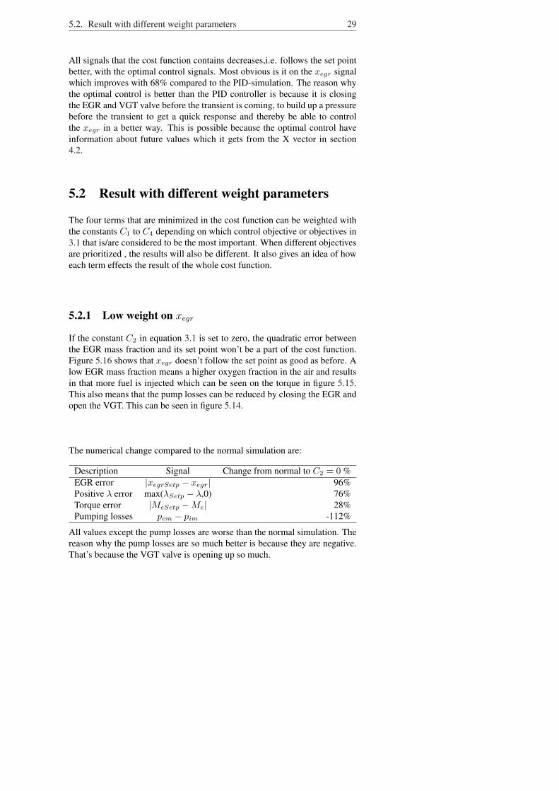
5.1.8 Torque

To get an understanding of how good uδ follows its set point compared toother simulations, the torque Me is the most appropriate parameter to use.Since uδSetp is a function of ne,Me and the pump losses, it will change forevery simulation and not be a constant parameter. MeSetp, on the other hand,is taken directly from the ETC cycle and is the same under all circumstancesand it is also the dominating factor in the function for uδSetp. Thereby uδ andMe will have the same principal appearance. This means that it will be easierto see how the set point is followed when it does not change. Figure 5.10shows that the optimal torque has a faster response than the PID simulation.The reason for this is the higher turbine speed in section 5.1.5.

5.1. Simulations 27

390 392 394 396 398 400 402 404 406 408 4101

1.5

2

2.5

3

3.5

4Lambda

Time (s)

λ Optimalλ PIDλ Setpλ Min

Figure 5.9: λ from the optimal control signals and λ from the PID-controllercompared to the set point and to λmin.

390 392 394 396 398 400 402 404 406 408 410

0

200

400

600

800

1000

1200

1400

1600

1800

2000

Time (s)

Nm

Me

Me Setpoint

Me Optimal

Me PID

Figure 5.10: The torque from the optimal control signals and from the PIDcontroller.


5.1.9 Intake- and exhaust manifold pressureFigure 5.11 shows that the difference between pim and pem, the pump loses,are smaller than it is with the PID regulator. The reason why the pumpinglosses is lower than in the PID simulation can be seen in figure 5.3. We cansee that the EGR valve is more open in our simulation compared to the PIDsimulation. The EGR valve also has a faster opening than the PID simulation.If the EGR valve is open, the pressure can not be built up which leads to lowerpumping losses.

390 392 394 396 398 400 402 404 406 408 4100

2

4

6

8

10

12

14

16

18x 10

4 Pumping Losses

Time (s)

Pa

p

em−p

im Optimal

pem

−pim

PID

Figure 5.11: Pump losses from the optimal control signals and from the PIDcontroller.

5.1.10 Time mean valueIt is interesting to see how much better optimal control is than a PID-controller.The time mean value of the different signals can be calculated by solving theintegral in equation(5.1), where y is the value of the signals for each timepoint. This gives the results that are presented in the following tabular.

y =1T

∫ t0+T

t0

ydt (5.1)

Description Signal Change from PID to optimal %EGR error |xegrSetp − xegr| -68%Positive λ error max(λSetp − λ,0) -14%Torque error |MeSetp −Me| -9%Pumping losses pem − pim -14%

5.2. Result with different weight parameters 29

All signals that the cost function contains decreases,i.e. follows the set pointbetter, with the optimal control signals. Most obvious is it on the xegr signalwhich improves with 68% compared to the PID-simulation. The reason whythe optimal control is better than the PID controller is because it is closingthe EGR and VGT valve before the transient is coming, to build up a pressurebefore the transient to get a quick response and thereby be able to controlthe xegr in a better way. This is possible because the optimal control haveinformation about future values which it gets from the X vector in section4.2.

5.2 Result with different weight parameters

The four terms that are minimized in the cost function can be weighted withthe constants C1 to C4 depending on which control objective or objectives in3.1 that is/are considered to be the most important. When different objectivesare prioritized , the results will also be different. It also gives an idea of howeach term effects the result of the whole cost function.

5.2.1 Low weight on xegr

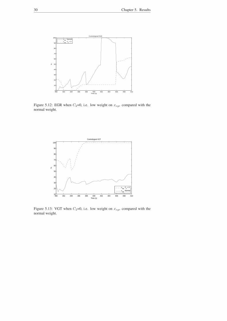
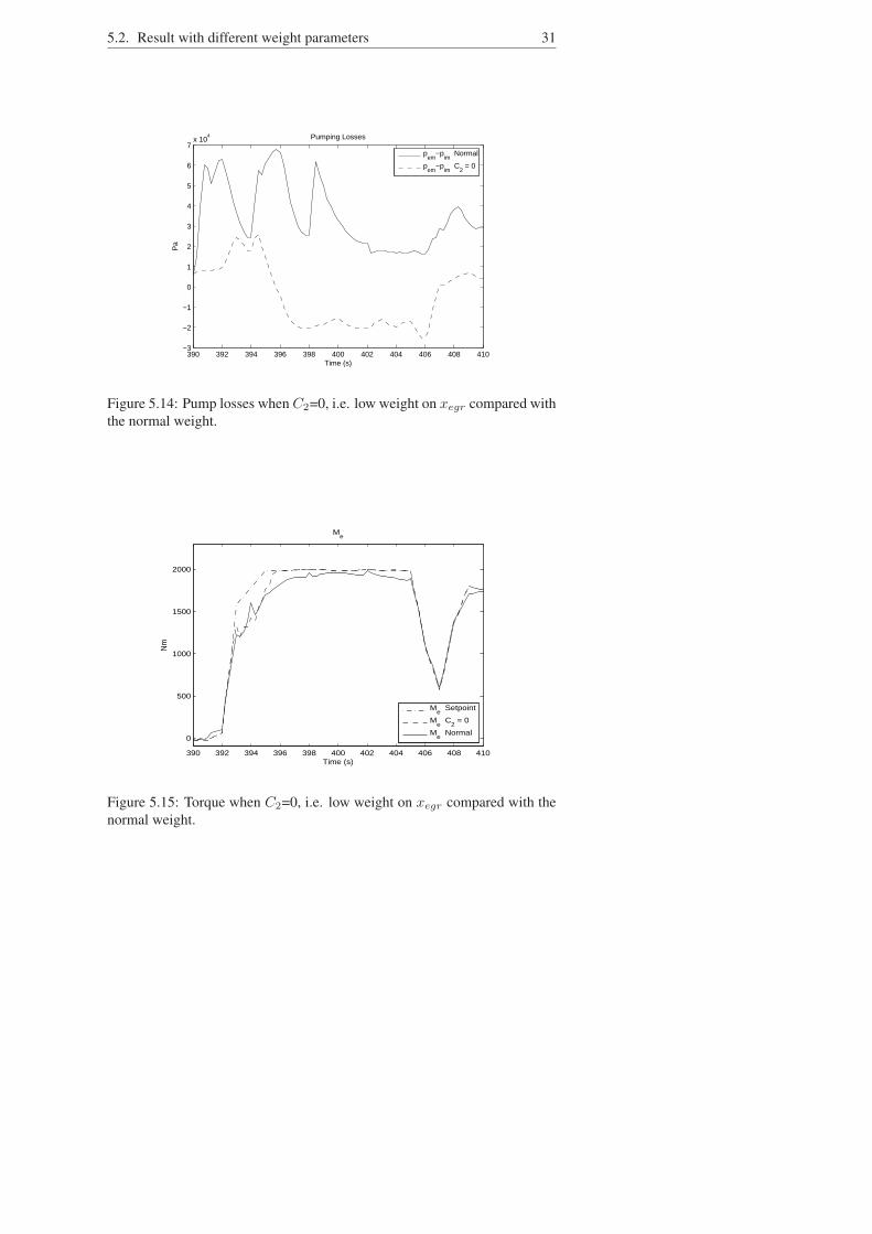
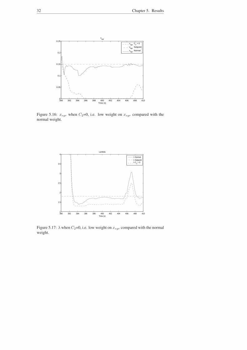
If the constant C2 in equation 3.1 is set to zero, the quadratic error betweenthe EGR mass fraction and its set point won’t be a part of the cost function.Figure 5.16 shows that xegr doesn’t follow the set point as good as before. Alow EGR mass fraction means a higher oxygen fraction in the air and resultsin that more fuel is injected which can be seen on the torque in figure 5.15.This also means that the pump losses can be reduced by closing the EGR andopen the VGT. This can be seen in figure 5.14.

The numerical change compared to the normal simulation are:

Description Signal Change from normal to C2 = 0 %EGR error |xegrSetp − xegr| 96%Positive λ error max(λSetp − λ,0) 76%Torque error |MeSetp −Me| 28%Pumping losses pem − pim -112%

All values except the pump losses are worse than the normal simulation. Thereason why the pump losses are so much better is because they are negative.That’s because the VGT valve is opening up so much.


390 392 394 396 398 400 402 404 406 408 4100

10

20

30

40

50

60

70

80

90


Time (s)

%

u

egr Normal

uegr

C2 = 0

Figure 5.12: EGR when C2=0, i.e. low weight on xegr compared with thenormal weight.

390 392 394 396 398 400 402 404 406 408 41010

20

30

40

50

60

70

80

90

100

Controlsignal VGT

Time (s)

%

uvgt

C2 = 0

uvgt

Normal

Figure 5.13: VGT when C2=0, i.e. low weight on xegr compared with thenormal weight.


390 392 394 396 398 400 402 404 406 408 410−3

−2

−1

0

1

2

3

4

5

6

7x 10

4 Pumping Losses

Time (s)

Pa

p

em−p

im Normal

pem

−pim

C2 = 0

Figure 5.14: Pump losses when C2=0, i.e. low weight on xegr compared withthe normal weight.

390 392 394 396 398 400 402 404 406 408 410

0

500

1000

1500

2000

Time (s)

Nm

Me

Me Setpoint

Me C

2 = 0

Me Normal

Figure 5.15: Torque when C2=0, i.e. low weight on xegr compared with thenormal weight.


390 392 394 396 398 400 402 404 406 408 4100

0.05

0.1

0.15

0.2

0.25

xegr

Time (s)

x

egr C

2 = 0

xegr

Setpoint

xegr

Normal

Figure 5.16: xegr when C2=0, i.e. low weight on xegr compared with thenormal weight.

390 392 394 396 398 400 402 404 406 408 4101

1.5

2

2.5

3

3.5

4Lambda

Time (s)

λ Normalλ Setpointλ C

2 = 0

Figure 5.17: λ when C2=0, i.e. low weight on xegr compared with the normalweight.


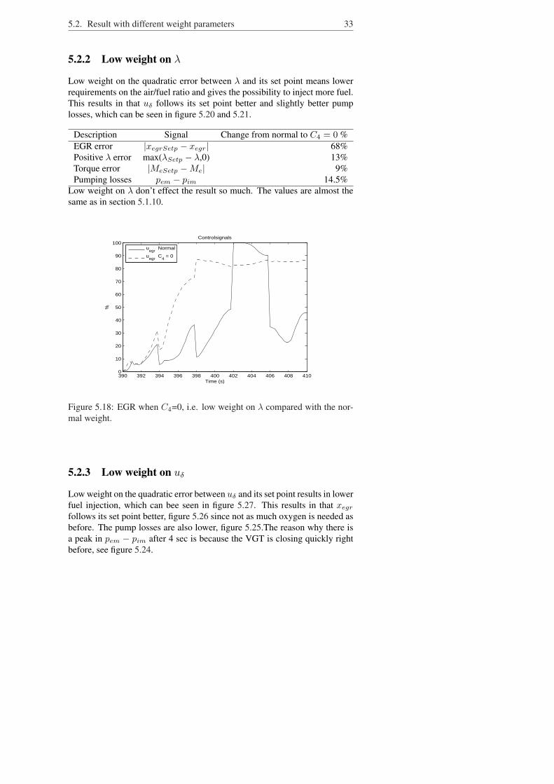
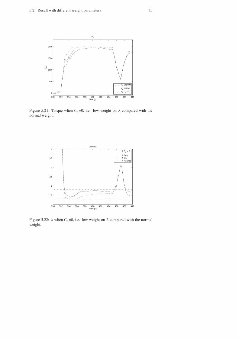
5.2.2 Low weight on λ

Low weight on the quadratic error between λ and its set point means lowerrequirements on the air/fuel ratio and gives the possibility to inject more fuel.This results in that uδ follows its set point better and slightly better pumplosses, which can be seen in figure 5.20 and 5.21.

Description Signal Change from normal to C4 = 0 %EGR error |xegrSetp − xegr| 68%Positive λ error max(λSetp − λ,0) 13%Torque error |MeSetp −Me| 9%Pumping losses pem − pim 14.5%

Low weight on λ don’t effect the result so much. The values are almost thesame as in section 5.1.10.

390 392 394 396 398 400 402 404 406 408 4100

10

20

30

40

50

60

70

80

90

100Controlsignals

Time (s)

%

u

egr Normal

uegr

C4 = 0

Figure 5.18: EGR when C4=0, i.e. low weight on λ compared with the nor-mal weight.

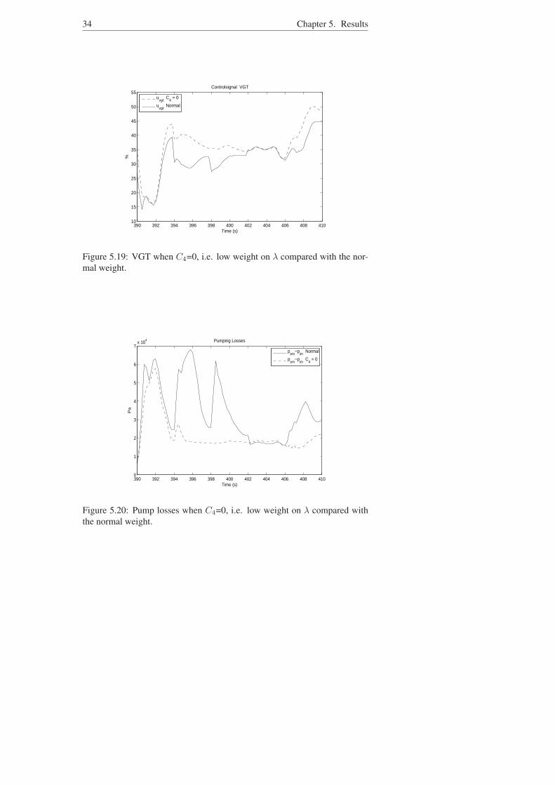
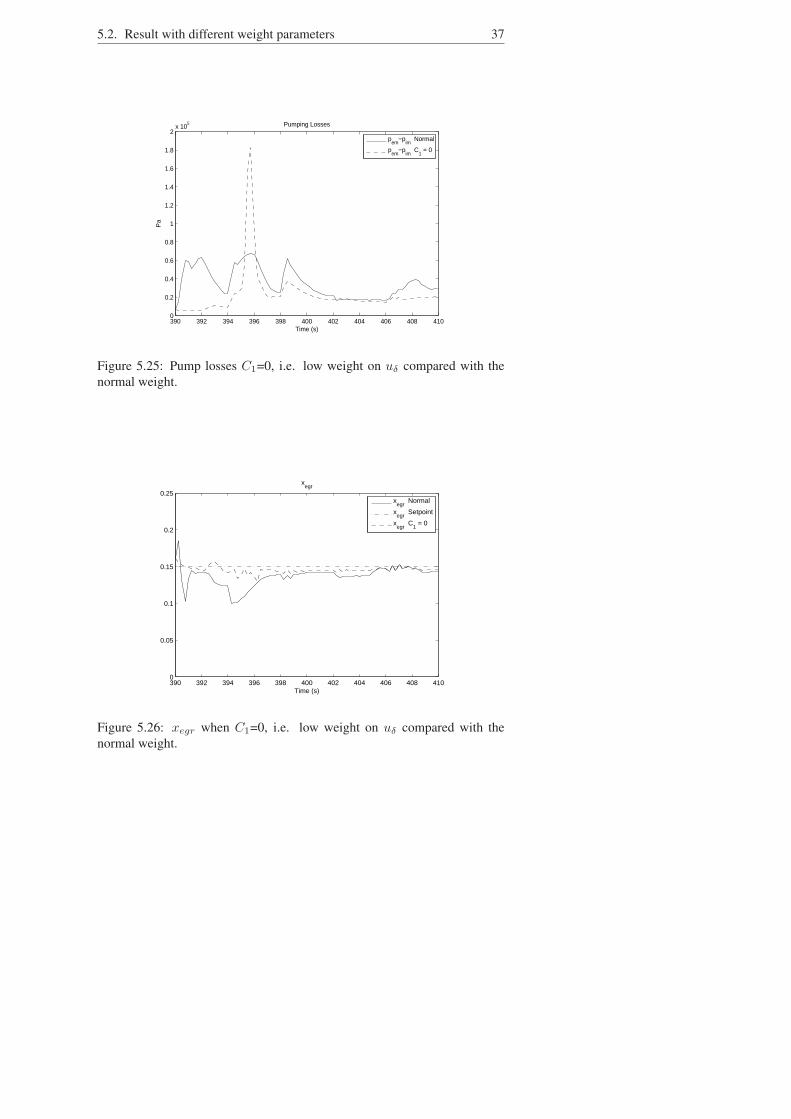
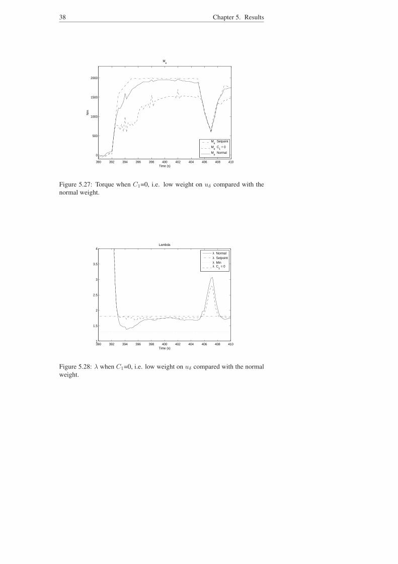
5.2.3 Low weight on uδ

Low weight on the quadratic error between uδ and its set point results in lowerfuel injection, which can bee seen in figure 5.27. This results in that xegr

follows its set point better, figure 5.26 since not as much oxygen is needed asbefore. The pump losses are also lower, figure 5.25.The reason why there isa peak in pem − pim after 4 sec is because the VGT is closing quickly rightbefore, see figure 5.24.


390 392 394 396 398 400 402 404 406 408 41010

15

20

25

30

35

40

45

50

55Controlsignal VGT

Time (s)

%

u

vgt C

4 = 0

uvgt

Normal

Figure 5.19: VGT when C4=0, i.e. low weight on λ compared with the nor-mal weight.

390 392 394 396 398 400 402 404 406 408 4100

1

2

3

4

5

6

7x 10

4 Pumping Losses

Time (s)

Pa

p

em−p

im Normal

pem

−pim

C4 = 0

Figure 5.20: Pump losses when C4=0, i.e. low weight on λ compared withthe normal weight.


390 392 394 396 398 400 402 404 406 408 410

0

500

1000

1500

2000

Time (s)

Nm

Me

Me Setpoint

Me Normal

Me C

4 = 0

Figure 5.21: Torque when C4=0, i.e. low weight on λ compared with thenormal weight.

390 392 394 396 398 400 402 404 406 408 4101

1.5

2

2.5

3

3.5

4Lambda

Time (s)

λ C

4 = 0

λ Setpλ Minλ Normal

Figure 5.22: λ when C4=0, i.e. low weight on λ compared with the normalweight.


390 392 394 396 398 400 402 404 406 408 4100

10

20

30

40

50

60

70

80

90


Time (s)

%

u

egr Normal

uegr

C1 = 0

Figure 5.23: EGR when C1=0, i.e. low weight on uδ compared with thenormal weight.

390 392 394 396 398 400 402 404 406 408 41010

20

30

40

50

60

70

80

90Controlsignal VGT

Time (s)

%

u

vgt Normal

uvgt

C1 = 0

Figure 5.24: VGT when C1=0, i.e. low weight on uδ compared with thenormal weight.


390 392 394 396 398 400 402 404 406 408 4100

0.2

0.4

0.6

0.8

1

1.2

1.4

1.6

1.8

2x 10

5 Pumping Losses

Time (s)

Pa

p

em−p

im Normal

pem

−pim

C1 = 0

Figure 5.25: Pump losses C1=0, i.e. low weight on uδ compared with thenormal weight.

390 392 394 396 398 400 402 404 406 408 4100

0.05

0.1

0.15

0.2

0.25

xegr

Time (s)

x

egr Normal

xegr

Setpoint

xegr

C1 = 0

Figure 5.26: xegr when C1=0, i.e. low weight on uδ compared with thenormal weight.


390 392 394 396 398 400 402 404 406 408 410

0

500

1000

1500

2000

Time (s)

Nm

Me

Me Setpoint

Me C

1 = 0

Me Normal

Figure 5.27: Torque when C1=0, i.e. low weight on uδ compared with thenormal weight.

390 392 394 396 398 400 402 404 406 408 4101

1.5

2

2.5

3

3.5

4Lambda

Time (s)

λ Normalλ Setpointλ Minλ C

1 = 0

Figure 5.28: λ when C1=0, i.e. low weight on uδ compared with the normalweight.


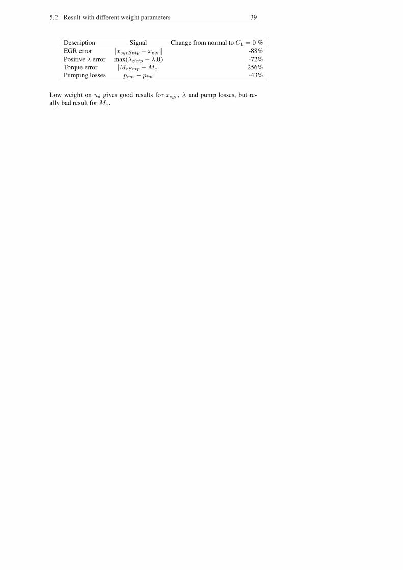
Description Signal Change from normal to C1 = 0 %EGR error |xegrSetp − xegr| -88%Positive λ error max(λSetp − λ,0) -72%Torque error |MeSetp −Me| 256%Pumping losses pem − pim -43%

Low weight on uδ gives good results for xegr, λ and pump losses, but re-ally bad result for Me.


5.3 Turbine efficiencyThe total turbine efficiency, ηtm consists of the turbine efficiency and me-chanical efficiency. Measurements show that ηtm is dependent of BSR (BladeSpeed Ratio) and the turbine speed ωt according to [1].

ηtm = ηtmmax − cm(BSR−BSRopt)2 (5.2)

BSR =Rtωt√

2cpeTem(1−Π1/γe

t )(5.3)

cm = cm1(ωt − cm2)cm3 (5.4)

Where ηtmmax is the maximal turbine efficiency, BSRopt is the optimal BSRvalue for maximal turbine efficiency and cm1,cm2,cm3 are parameters for themodel for cm.To get a view of how important the turbine efficiency is for the optimization,the parameter cm1, which variates the mechanical losses in equation 5.4 canbe changed. A high cm1 gives a deterioration of the conditions because thelosses is assumed to be higher. It is now possible to get an opinion of howimportant this parameter is for the system. If the efficiency is important forthe optimization , the difference between a large and small cm1 should belarge, i.e. the sensitivity of this parameter is significant.

5.3. Turbine efficiency 41

390 392 394 396 398 400 402 404 406 408 4100.2

0.3

0.4

0.5

0.6

0.7

0.8

0.9

1

BSR NormalBSR

OptBSR Optimal c

m1 * 1.2

BSR PID

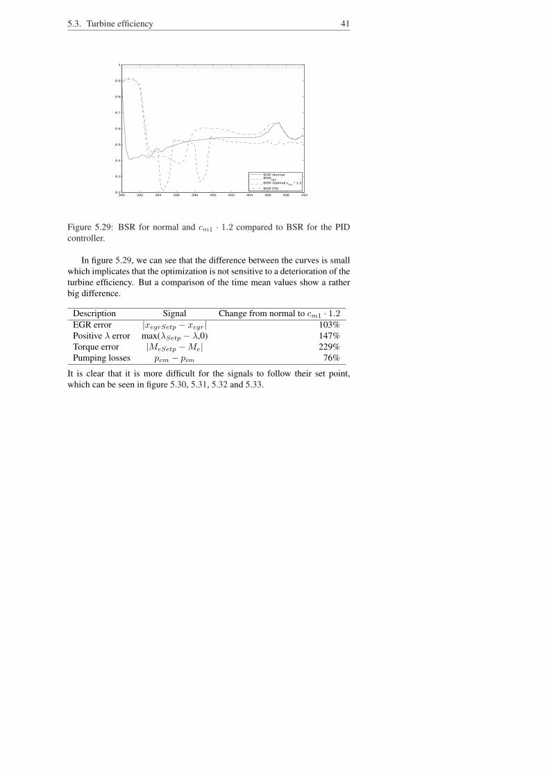
Figure 5.29: BSR for normal and cm1 · 1.2 compared to BSR for the PIDcontroller.

In figure 5.29, we can see that the difference between the curves is smallwhich implicates that the optimization is not sensitive to a deterioration of theturbine efficiency. But a comparison of the time mean values show a ratherbig difference.

Description Signal Change from normal to cm1 · 1.2EGR error |xegrSetp − xegr| 103%Positive λ error max(λSetp − λ,0) 147%Torque error |MeSetp −Me| 229%Pumping losses pem − pim 76%

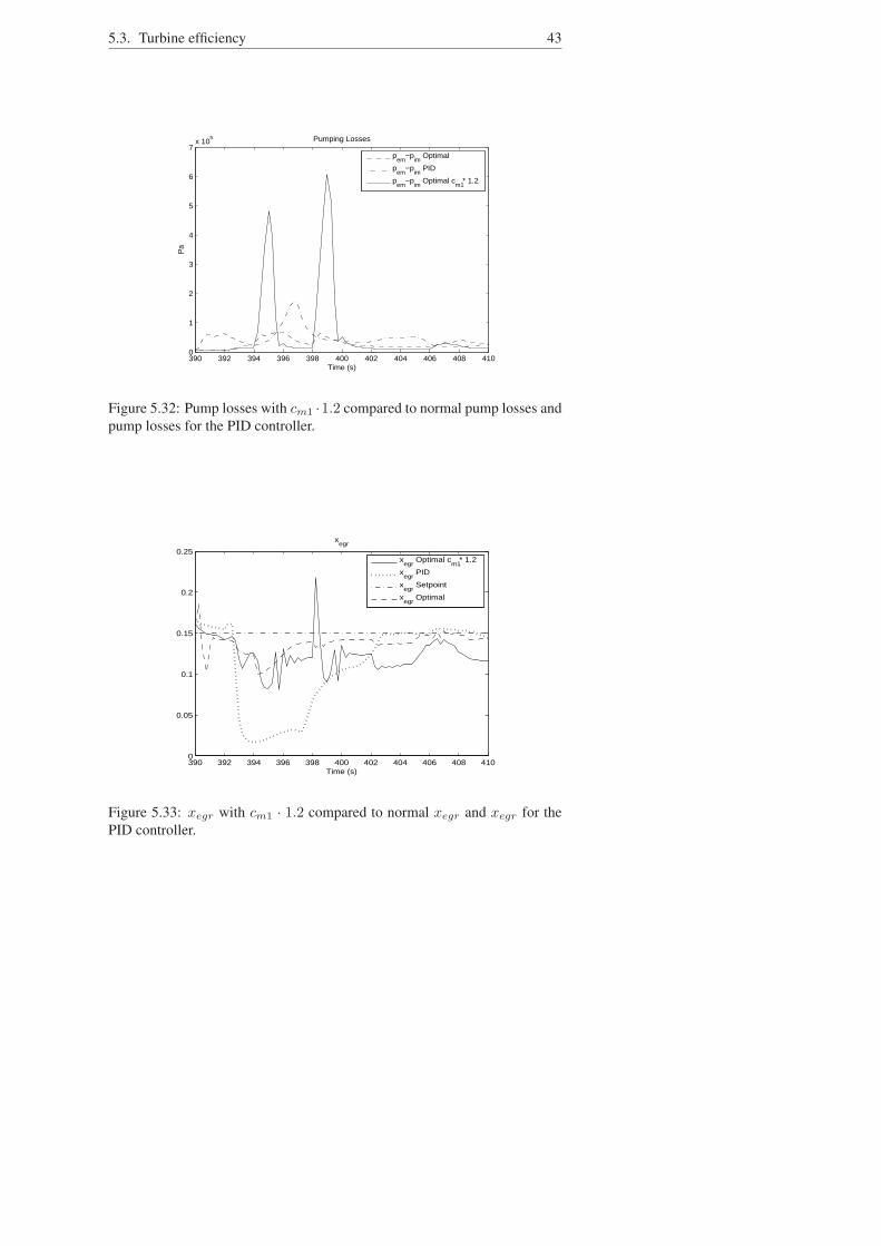
It is clear that it is more difficult for the signals to follow their set point,which can be seen in figure 5.30, 5.31, 5.32 and 5.33.


390 392 394 396 398 400 402 404 406 408 4101

1.5

2

2.5

3

3.5

4λ

Time (s)

λ Optimal c

m1 * 1.2

λ PIDλ Setpointλ Minλ Optimal

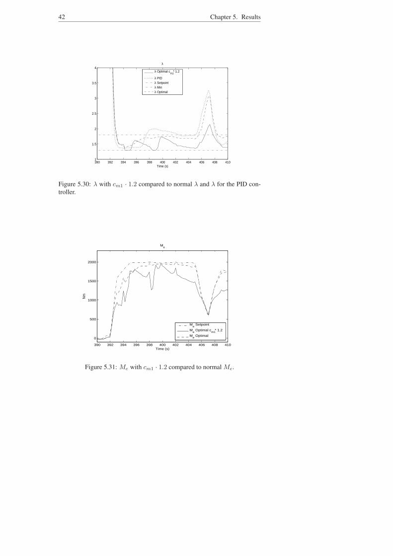
Figure 5.30: λ with cm1 · 1.2 compared to normal λ and λ for the PID con-troller.

390 392 394 396 398 400 402 404 406 408 410

0

500

1000

1500

2000

Time (s)

Nm

Me

Me Setpoint

Me Optimal c

m1 * 1.2

Me Optimal

Figure 5.31: Me with cm1 · 1.2 compared to normal Me.

5.3. Turbine efficiency 43

390 392 394 396 398 400 402 404 406 408 4100

1

2

3

4

5

6

7x 10

5 Pumping Losses

Time (s)

Pa

p

em−p

im Optimal

pem

−pim

PID

pem

−pim

Optimal cm1

* 1.2

Figure 5.32: Pump losses with cm1 ·1.2 compared to normal pump losses andpump losses for the PID controller.

390 392 394 396 398 400 402 404 406 408 4100

0.05

0.1

0.15

0.2

0.25

xegr

Time (s)

x

egr Optimal c

m1 * 1.2

xegr

PID

xegr

Setpoint

xegr

Optimal

Figure 5.33: xegr with cm1 · 1.2 compared to normal xegr and xegr for thePID controller.


5.4 Compressor efficiencyIn the same way that it is possible to make worse conditions by changingthe parameter cm1 in the turbine, it is possible to make better conditions bychanging the maximal efficiency in the compressor and see if the transientimproves. The compressor efficiency,ηc can, according to [1], be describedas:

ηc = ηcmax − χT Qcχ (5.5)

χ is a vector that contains the inputs

χ = [Wc −Wopt, πc − πcopt]T (5.6)

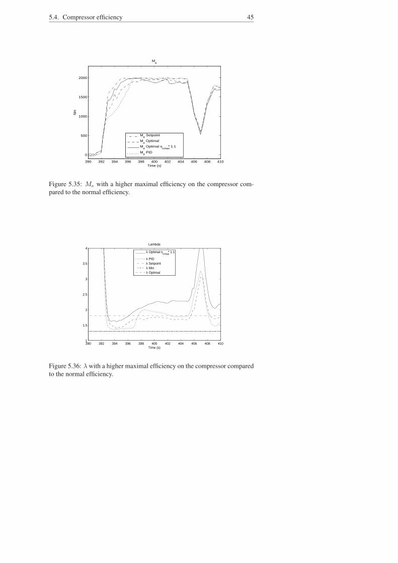
and Qc is a matrix which consists of three parameters.The transients with a higher maximal efficiency can be seen in figure 5.34,5.35, 5.36 and 5.37

390 392 394 396 398 400 402 404 406 408 4100

2

4

6

8

10

12

14

16

18x 10

4 Pumping Losses

Time (s)

Pa

p

em−p

im Optimal

pem

−pim

PID

pem

−pim

Optimal ηcmax * 1.1

Figure 5.34: Pump losses with a higher maximal efficiency on the compressorcompared to the normal efficiency.

And the change in % is

Description Signal Change from normal to ηcmax · 1.1EGR error |xegrSetp − xegr| -60%Positive λ error max(λSetp − λ,0) -80%Torque error |MeSetp −Me| -26%Pumping losses pem − pim -24%

5.4. Compressor efficiency 45

390 392 394 396 398 400 402 404 406 408 410

0

500

1000

1500

2000

Time (s)

Nm

Me

Me Setpoint

Me Optimal

Me Optimal η

cmax * 1.1

Me PID

Figure 5.35: Me with a higher maximal efficiency on the compressor com-pared to the normal efficiency.

390 392 394 396 398 400 402 404 406 408 4101

1.5

2

2.5

3

3.5

4Lambda

Time (s)

λ Optimal η

cmax * 1.1

λ PIDλ Setpointλ Minλ Optimal

Figure 5.36: λ with a higher maximal efficiency on the compressor comparedto the normal efficiency.


390 392 394 396 398 400 402 404 406 408 4100

0.05

0.1

0.15

0.2

0.25

xegr

Time (s)

x

egr Optimal η

cmax * 1.1

xegr

PID

xegr

Setpoint

xegr

Optimal

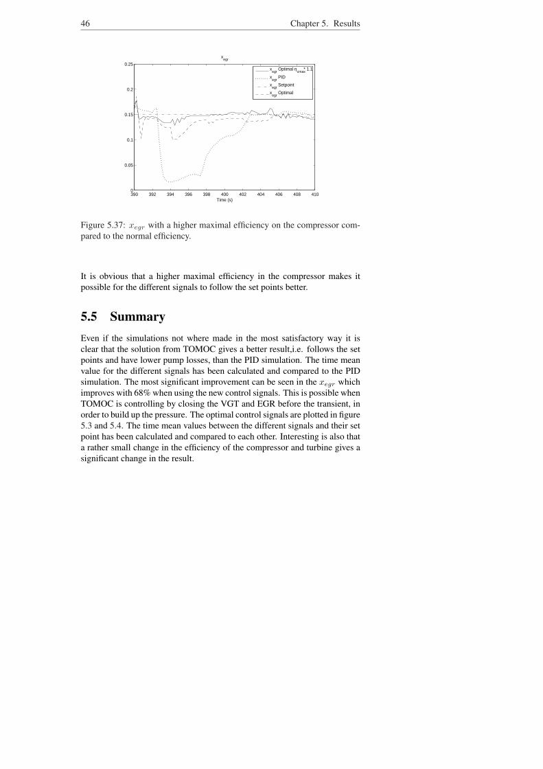
Figure 5.37: xegr with a higher maximal efficiency on the compressor com-pared to the normal efficiency.

It is obvious that a higher maximal efficiency in the compressor makes itpossible for the different signals to follow the set points better.

5.5 SummaryEven if the simulations not where made in the most satisfactory way it isclear that the solution from TOMOC gives a better result,i.e. follows the setpoints and have lower pump losses, than the PID simulation. The time meanvalue for the different signals has been calculated and compared to the PIDsimulation. The most significant improvement can be seen in the xegr whichimproves with 68% when using the new control signals. This is possible whenTOMOC is controlling by closing the VGT and EGR before the transient, inorder to build up the pressure. The optimal control signals are plotted in figure5.3 and 5.4. The time mean values between the different signals and their setpoint has been calculated and compared to each other. Interesting is also thata rather small change in the efficiency of the compressor and turbine gives asignificant change in the result.

Chapter 6

Conclusions

In this chapter an analysis of the results of the different signals and simula-tions is made.

6.1 Cost functionThe assignment has been to find the optimal control signals by minimizing thecost function 3.1. The different parameters have been weighted in differentways and several simulations has been made. The most important parametersin the cost function that have been weighted are:

• The quadratic error between the fuel injection and its set point. Whenanalyzing the results it is better to analyze the error between the torqueand its set point instead, see section 5.1.8.

• The quadratic error between the mass fraction in the EGR valve, xegr,and its set point.

• The quadratic error between λ and its set point. Consideration to that itis nothing negative with a large λ has been taken.

6.2 ResultsIf we study the results in chapter 5, we can come to the conclusion that op-timal control with TOMOC gives a better results from than a PID regulator,even though the results are quite similar. The improvement for the time meanvalues of the different signals can be seen in the tabulars in chapter 5. It isalso interesting to see that a rather small change of the parameters cm1 andηcmax in section 5.3 and 5.4 gives a significant change in the result. The mostsignificant improvement is that the xegr follows its set point 68% better than

47

48 Chapter 6. Conclusions

the PID simulation, this is because TOMOC can prepare the system for thedifferent transients.

6.3 Control signals

6.3.1 Is this the optimal control?The optimal control signals that have been calculated in TOMOC can be seenin figure 5.3 and 5.4. But can we be sure that this really are the optimal con-trol way to control the two signals? The answer to that question is no. Sincewe do not have any possibility to control if the solution is a global or localoptimum, we can not exclude that there could be a better way to control thesignals. It is also unclear how the use of the initial values have effected theresults. We can also see that the big difference between our simulation andthe PID simulation is the control of the EGR valve. The VGT signal is almostthe same in the two simulations but the EGR shows some interesting differ-ences. It seems to be desirable to open up the EGR valve more and faster inorder to lower the exhaust manifold pressure. That leads to a lower turbinespeed and a smaller amount of air can be pressed into the engine by the turbo,which leads to a lower pressure in the intake manifold. In that way the pumplosses are reduced.

6.4 SimulationsSince there have been problems with long simulation times, and that the sim-ulations crashes if the sample time is to high, the 20 sec long simulations havebeen divided into five 4 sec long simulations. This should not give so muchdifferent result than one 20 sec long simulation. However, in some intervalsthe control signals have some tops and dips that is a direct result of this.Why the simulations crash when the sample time is to high, we don’t know.Normally a simulation with high sample time would be more accurate than asimulation with low sample time. Probably the simulations do not convergebecause of some kind of numerical difficulties.

Chapter 7

Future Work

In this chapter further work to this master’s thesis is discussed.

7.1 OptimizationThe mayor problem in this work has been the long simulation time and it isdesirable to short down this time. It would also be desirable to simulate witha better sample time, i.e. simulate with more segments. The accuracy wouldthen be better and the result more precise.Something that would be interesting is to compare fmincon with an otherkind of solver. That it is a very important part of the optimization but stilldifficult to say if fmincon is a good choice or not. An other solver may givea different result.Try to use other methods instead of trapeze method, like Euler which alreadyis implemented in TOMOC, to make the optimization problem discrete.TOMOC is very sensitive for different initial values. If an observer whichcould calculate future values was made, these values could then be used asinitial values. This would mean that the simulation didn’t have to follow thePID simulation at all. There would be a better chance that a global optimumwas found.If TOMLAB is available, it would of course be interesting to see the resultwhen using that.

49

References

[1] J.Wahlsrom. Modeling of a diesel engine with VGT and EGR. Tech-nical report, Division of Vehicular Systems, Linkopings University,Linkopings Universitet, Linkoping, Sweden, 2005.

[2] A. Lagerberg. Open-loop optimal control of a backlash traverse. Tech-nical report, Department of Signals and Systems,Chalmers University ofTechnologi, School of engineering Jonkoping University, 2004.

[3] Lennart Ljung and Torkel Glad. Reglerteori. 3 edition, 1997.

[4] Lars Nielsen and Lars Eriksson. Course material Vehicular System. 2004.

[5] T.Johansson. System analysis of a diesel engine with VGT andEGR. Master’s thesis LiTH-ISY-EX-3714, , Linkopings Universitet,Linkoping, Sweden, January 2005.

[6] C. Vigild. The Internal Combustion Engine Modelling, Estimation andControl Issues. PhD thesis, Technical University of Denmark, Lyngby,2001.

[7] Johan Wahlstrom, Lars Eriksson, Lars Nielsen, and Magnus Pettersson.PID controllers and their tuning for EGR and VGT control in diesel en-gines. IFAC World Congress, Prague, Czech Republic, 2005.

50

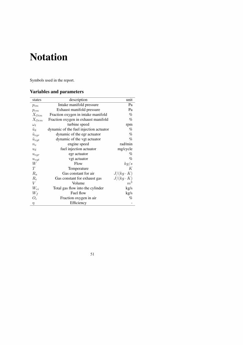
Notation

Symbols used in the report.

Variables and parametersstates description unitpim Intake manifold pressure Papem Exhaust manifold pressure PaXOim Fraction oxygen in intake manifold %XOem Fraction oxygen in exhaust manifold %ωt turbine speed rpmuδ dynamic of the fuel injection actuator %uegr dynamic of the egr actuator %uvgt dynamic of the vgt actuator %ne engine speed rad/minuδ fuel injection actuator mg/cycleuegr egr actuator %uvgt vgt actuator %W Flow kg/sT Temperature KRa Gas constant for air J/(kg ·K)Re Gas constant for exhaust gas J/(kg ·K)V Volume m3

Wei Total gas flow into the cylinder kg/sWf Fuel flow kg/sOc Fraction oxygen in air %η Efficiency -

51

Appendix A

TOMOC Manual

A.1 Introduction

This is a introduction to the TOMOC version that was made, by Adam Lager-berg, special for Linkopings university. It is written mainly to give futureusers a help to get started with the program. We have described how wesolved different problems without saying that our method is the only way orthe best way to solve the problem.

TOMOC consists of several different m-files which are used together withfmincon to solve the optimal control problem.There are both problem specific and not problem specific files. The problemspecific functions,i.e. the functions that must be changed to match the spe-cific problem, are describes in the following sections.

A.2 Tomlkpg1start

The TOMOC template used here is originally made to solve a specific prob-lem so many things have to be changed to make it work for other problems.For the problem in this thesis is not possible to make a setup on matrix formso it has a different setup than the original. This introduction is an effort toexplain the changes necessary to get a more complex model to work withinthe template. Tomlkpg1start which is the main script in TOMOC is builtaround fmincon and calls on the other functions. It defines time interval,sample time, simple bounds etc..

52

A.2. Tomlkpg1start 53

A.2.1 PhasesThe number of phases is described by (P.user.nph) in TOMOC. If thedynamic trajectory of the system differs over time it is possible to divide itinto different parts. Each phase will correspond with the specific dynamicsand will be treated as a separate systems which are linked together. Also dif-ferent boundary conditions and constraints can be given for each phase. Theadvantage with this setup is that it makes it easy to handle different dynamicswithin the same area problem.

A.2.2 StatesThe number of states is in TOMOC defined by (P.user.phph.ny). Thisvalue is used to decide the size of the vector X and X0.

A.2.3 Control signalsThe number of control signals is defined by (P.user.phph.nu).Thisvalue is used to decide the size of the vector X and X0. Segments on phase(P.user.phph.ns). This parameter decides how many segments to becalculated with on each phase. Indirectly this will also decide the sample timefor the run if the goal is to minimize over a timespan. If the goal is to mini-mize time this will indicate the accuracy. It is convenient to start with a smallvalue and then iteratively increase it to improve the accuracy of the solution.

A.2.4 Initial valuesThe initial values are in TOMOC defined by(P.user.phph.(xi , ui))and (P.user.phph.(xf , uf)). It is important that this value is agood guess if a correct solution will be achieved since the program searchesfor a minimum around this point. It is not possible to know if this is a globalor local minimum. This value is a constraint and will be the fixed value forstates and control signal in the first and/or last point of the calculation. It ispossible to set (xi , ui) for one or more whole segments in the X vector or pickout specific values in one or more segments. If no points are going to be usedset to infinity. This value is used to calculate the X0 vector how are inter-polate from start to final, if no final exists the X0 vector will be interpolatedfrom final to final. If nothing is provided zeros are assumed. Initial values areto be set as a transposed vector or matrix.

A.2.5 Time constraintsThe time interval for the calculation is set in P.user.phph.Dtconstr.The time is a part of the X vector and is a constraint value. Set to infinity ifa minimal time calculation is wanted, in this case time will not be used as a

54 Appendix A. TOMOC Manual

constraint. The sample time will be time divided with number of segments.P.user.Dttotconstr is total time for all phases.

A.2.6 Initial guessesA guess of the initial and final values can be set in P.user.phph.(xig, uig) and P.user.phph.(xfg , ufg). It is favorable to use thisfunction if a good guess exists for the whole vector or a part of it. If thesevalues are set they will act as start points for the X vector and they will notbe set as constraints. This will reduce the convergence speed since the NPLsolution is dependent on a good initial value. If a good guess exists for thewhole vector it would be possible to directly replace it with X0 without us-ing TomocInitguess, a constraint initial guess for the first point in the vectorwould still be necessary since it is used on other places than TomocInitguess.Simple bounds LB and UB restrains the values between two points for eachstate and control signal. If LB = UB a fixed value is obtained. Bounds can bevectors or scalers, and can be set for every segment. It is e g possible to getthe bounds to follow a trajectory by defining a vector and letting LB = UB

X vector

The vector used by the solver is called X and contains time, dynamic statesand control signals. The initial X vector is created in Tomocinitguessfrom the initial values defined in tomlkpgstart. The values are interpo-lated from initial to final to fit the number of segments on the phase. The Xvector is structured in the following way

X = [X(1), X(2), ..., X(nph)]

where X(p) is the vector for phase p, p = 1, 2..., nph

X(p) = [∆t, x1, u1, x2,u2, ..., xns+1, uns+1]

where

∆t is the time on phase p, xkis the state variable and uk is the control signalvector in each segment node k,k = 1, 2, .., ns + 1

xk = [xk1 , xk

2 , ..., xkny

]uk = [uk

1 , uk2 , ..., uk

nu]

For example assume:number of segments = 3number of phases = 1

A.3. tomlkpg1fun 55

number of states = 2number of control signals = 2

the created vector is linearly interpolated from (xi, ui) to (xf , uf ) so that

X0 = [∆t, x11, x

12, u

11, u

12, x

21, x

22, u

21, x

31, x

32, u

31, u

32, x

41, x

42, u

41, u

42]

And if a prior X exists in workspace Tomocinitguess will use this asa new starting guess. If the number of segments have been changed since lastrun a new X0 whit the right length will be interpolated from the prior gridpoints. This is of importance since the convergence speed of the solution isdependent of a good initial value. It is even possible that no solution at all isfound if the initial values are to bad. It also possible to set only a few individ-ual initial values and let the rest be zeros. This is possible by using guessedvalues. If the (xi, xf) vector is set to infinite, and guessed values provided in(xig, xfg) are used, all values not used in (xig, xfg) will be set to zeros andonly the guessed values are used.

Upper-and lower bounds

The states and control signals can be restricted to not exceed or be belowa certain value. This will be done for every state and control signal for allsegments by controlling the correct element in the X vector.With these boundsit is possible to give a state a specific value during the whole simulation bysetting UB=LB.

Structs

The struct P contains data from user defined functions and statemaker.

Optimset

The function optimset creates a structure that pass on a input argument to thefmincon function. This gives the user a possibility to change the conditionsfor the simulation. For example number of iterations, termination conditions,display options can be set. Also gives the opportunity to choose which nu-merical method the solver should use.

A.3 tomlkpg1funContains the cost function and all the dynamics that is required to calculatethe cost function. The function picks out indexes of control signals and statesat each time point. The index correspond to the place in the vector X wherethe signal is located. This makes it possible to sort out the right signal from


vector X needed to calculate the cost function. The result is a vector corre-sponding to chosen signal whit length equal to number of segments. If othervariables is needed to calculate the cost function it is necessary to estimatethem here by using the generated vectors.Example:The needed signal is control signal 1 (u1) then index u1 isiu1=iDt+P.user.ph(ph).ny+1+P.user.ph(ph).nyu

*(0:P.user.ph(ph).ns)where iDt is time which is placed first in the vector for each phase.

P.user.ph(ph).ny is number of states on each phase. (1)P.user.ph(ph).nyu is total number of signals on each phase. (2)P.user.ph(ph).ns is number of segments on each phase. (3)if (1) = 4 , (2) = 2 , (3) = 2 then the result is a vector which contains index foru1 iu1 = [6 12 18] then it is straight forward to pick out the signal from the Xvector.

A.4 tomlkpg1dynfuntomlkpg1dynfun contains the dynamics to be used in optimization. If thesystem is linear and written on the form x = Ax + Bu it is possible to imple-ment it on matrix form (see [2]). If it is a non linear problem , which can’tbe written on matrix form, a separate function which contains the dynamicscan be written to solve the problem. In this case dynfun should work as a linkbetween Tomoc and the dynamics. Every time Tomoc calls upon dynfun theinformation should be passed on to the dynamics function and the answer re-turn the same way. This is very straightforward to implement, just exchangethe existing dynamics in template with the new dynamics function so that in-stead of f = Ax+Bu you get f = dynamicsfunction(x,u).

It can be a good idea to weight the dynamics so that the values outside the dy-namics function are approximately the same size. This is done to prevent thatbig units has more influence than small units in the handling of constraints.The benefits is a greater convergence speed. The easiest way to do this is tomultiply the ingoing values to the dynamics function whit a diagonal matrixcontaining numbers in the same range as states and control signals. Thenmultiply outgoing values with the inverse of the same matrix.

ExampleThe values that are going in and coming out from the function should be ap-proximately the same size, but the values used by the dynamics should havethe proper value. Hence the values of inputs to the dynamics should be multi-

A.5. tomlkpg1initpar 57

plied with a vector (x0, u0) and values of the outputs from the dynamics mustbe divided with x0. An easy way to do this is as following

s = diag(x0)s−1 = s-1v = u0 · ux = s−1· dynamics(s · x, v)

Since the dynamics function are called upon many times during a simula-tion it is computably necessary to set the used constants as global, so thatthey are available for calculations at all times without the need to load themat each call to the function. One way to do this is to run a initialization filewere the needed constants are assigned a global value. Any assignment to thatvariable, in any function, then is available to all the other functions declaringit as global.

A.5 tomlkpg1initpar

Initialization of problem specific parameter values. Since this file uses thestates on matrix form, it should be replaced/changed if the problem is nonlinear.

A.6 tomlkpg1constraints

The file Tomlkpg1constraintsmakes it possible to set problem specific(non)linear constraints.

The problem independent functions are described in the following sections.

A.7 tomocinitguess

The file Tomocinitguess constructs an initial guess by linear interpola-tion between parameters set in start (see X). Even thou the file is said to beproblem independent it has to be changed to fit the problem specifics. Thetemplate is made to work with two states and one control signal, if this differsit has to be changed. Guesses for u should be rewritten in the same form asfor states and the linear interpolation part has to be expanded to fit the newproblem.


A.8 tomocconphMulti-phase constraint definition. This function calls tomoccon (see A.9)once for each phase, and then assembles all constraints into one vector. Thestate and control variables on each phase are assumed to be the same, and tobe continuous over the phase boundaries. TOMLAB uses one vector both forequality and inequality constraints. Special constrains equations are used forthis.

A.9 tomocconThis function is called by tomocconph once for each phase and calculatesconstraints for the boundary values, initial and final time. The function cal-culate the constraints vector ceq. It is calculated in different parts, some inloops and some in sequence after each other. Every calculation part uses thetemporary variable ceqk. After that the vector is put together gradually withtomocconph.

A.10 tomocpostprocThis function handles the result vector X and reshapes it to a matrix , xr, con-taining states, control signals and time. This makes it easy to pick out thewanted variables for use in plot functions. The result is also used as initialguess if the workspace is not cleared for a second run.

Copyright

Svenska

Detta dokument halls tillgangligt pa Internet - eller dess framtida ersattare -under en langre tid fran publiceringsdatum under forutsattning att inga extra-ordinara omstandigheter uppstar.

Tillgang till dokumentet innebar tillstand for var och en att lasa, ladda ner,skriva ut enstaka kopior for enskilt bruk och att anvanda det oforandrat forickekommersiell forskning och for undervisning. Overforing av upphovsrattenvid en senare tidpunkt kan inte upphava detta tillstand. All annan anvandningav dokumentet kraver upphovsmannens medgivande. For att garantera aktheten,sakerheten och tillgangligheten finns det losningar av teknisk och administra-tiv art.

Upphovsmannens ideella ratt innefattar ratt att bli namnd som upphovs-man i den omfattning som god sed kraver vid anvandning av dokumentet paovan beskrivna satt samt skydd mot att dokumentet andras eller presenterasi sadan form eller i sadant sammanhang som ar krankande for upphovsman-nens litterara eller konstnarliga anseende eller egenart.

For ytterligare information om Linkoping University Electronic Press seforlagets hemsida: http://www.ep.liu.se/

English

The publishers will keep this document online on the Internet - or its possiblereplacement - for a considerable time from the date of publication barringexceptional circumstances.

The online availability of the document implies a permanent permissionfor anyone to read, to download, to print out single copies for your own useand to use it unchanged for any non-commercial research and educationalpurpose. Subsequent transfers of copyright cannot revoke this permission.All other uses of the document are conditional on the consent of the copy-right owner. The publisher has taken technical and administrative measuresto assure authenticity, security and accessibility.

According to intellectual property law the author has the right to be men-tioned when his/her work is accessed as described above and to be protectedagainst infringement.

For additional information about the Linkoping University Electronic Pressand its procedures for publication and for assurance of document integrity,please refer to its WWW home page: http://www.ep.liu.se/

optimal control of a diesel engine with vgt and egr · optimal control of a diesel engine with vgt...

Documents