optimal control for jump processes, hjb...
TRANSCRIPT

Optimal controlfor jump
processes,HJB equations
Jakub Petrasek
Introduction
Motivation
Levy processes
Optimal Control
Model set-up
Dynamicprogrammingprinciple
Application
Formulation ofproblem
Application ofdynamicprogrammingprinciple
Comparison withno-jump case
Maximmumprinciple
Model set-up
Optimalitycondition
Relation todynamicprogramming
Bibliography
Optimal control for jump processes,HJB equations
Jakub Petrasek
Department of Probability and Mathematical StatisticsFaculty of Mathematics and Physics, Charles University in Prague
Seminar in Stochastic Modelling in Economics and Finance
January 10, 2011

Optimal controlfor jump
processes,HJB equations
Jakub Petrasek
Introduction
Motivation
Levy processes
Optimal Control
Model set-up
Dynamicprogrammingprinciple
Application
Formulation ofproblem
Application ofdynamicprogrammingprinciple
Comparison withno-jump case
Maximmumprinciple
Model set-up
Optimalitycondition
Relation todynamicprogramming
Bibliography
Outline
1 IntroductionMotivationLevy processes
2 Optimal ControlModel set-upDynamic programming principle
3 ApplicationFormulation of problemApplication of dynamic programming principleComparison with no-jump case
4 Maximmum principleModel set-upOptimality conditionRelation to dynamic programming
1

Optimal controlfor jump
processes,HJB equations
Jakub Petrasek
Introduction
Motivation
Levy processes
Optimal Control
Model set-up
Dynamicprogrammingprinciple
Application
Formulation ofproblem
Application ofdynamicprogrammingprinciple
Comparison withno-jump case
Maximmumprinciple
Model set-up
Optimalitycondition
Relation todynamicprogramming
Bibliography
Economic model
At each t ≥ 0 an agent owns a capital Xt by investing in two assets
a riskfree bond that pays interest rate r ,
dBt = rBtdt.
a risky asset with dynamics (geometric Brownian motion +jumps)
dSt = S(t−)
(αdt + σdWt +
∫ ∞−1
zN(dt,dz)
).
At each t ≥ 0 an agent controls
the number of stocks ∆t in his portfolio,
and possibly consumption Ct .
2

Optimal controlfor jump
processes,HJB equations
Jakub Petrasek
Introduction
Motivation
Levy processes
Optimal Control
Model set-up
Dynamicprogrammingprinciple
Application
Formulation ofproblem
Application ofdynamicprogrammingprinciple
Comparison withno-jump case
Maximmumprinciple
Model set-up
Optimalitycondition
Relation todynamicprogramming
Bibliography
Admissible strategies
Definition
A strategy (∆t , t ≥ 0) is admissible if
1 it is predictable,
2 the portfolio (Xt , t ≥ 0) is self-financing, i.e.
dXt = ∆tdSt + (Xt −∆tSt)dBt .
We denote the set of admissible strategies by A(x) for a given capitalX0 = x .
We can substitute for dSt and dBt and obtain
dXt = ∆tSt−
((α− r)dt + σdWt +
∫ ∞−1
zN(dt,dz)
)+ rXtdt.
3

Optimal controlfor jump
processes,HJB equations
Jakub Petrasek
Introduction
Motivation
Levy processes
Optimal Control
Model set-up
Dynamicprogrammingprinciple
Application
Formulation ofproblem
Application ofdynamicprogrammingprinciple
Comparison withno-jump case
Maximmumprinciple
Model set-up
Optimalitycondition
Relation todynamicprogramming
Bibliography
Objective of investment
The objective of an agent is to maximize his utility from investmentsby using admissible strategies ∆t(∆t ,Ct). His aim is
1 to maximize his consumption over infinite horizon
sup(∆t ,Ct)∈A(x)
∫ ∞0
e−βtE U(Ct)dt, (1.1)
where β is a discount factor
2 to maximize his terminal utility of terminal wealth in a givenhorizon T
sup∆t∈A(x)
E U(XT ), (1.2)
3 combination of the first two
sup(∆t ,Ct)∈A(x)
E U(XT ) +
∫ T
0
e−βtE U(Ct)dt
. (1.3)
4

Optimal controlfor jump
processes,HJB equations
Jakub Petrasek
Introduction
Motivation
Levy processes
Optimal Control
Model set-up
Dynamicprogrammingprinciple
Application
Formulation ofproblem
Application ofdynamicprogrammingprinciple
Comparison withno-jump case
Maximmumprinciple
Model set-up
Optimalitycondition
Relation todynamicprogramming
Bibliography
Levy process - definition
Definition
Let(
Ω,F , Ftt≥0 ,P)
be a filtered probability space. An adapted
process Lt is called a Levy process if it is continuous in probabilityand has stationary, independent increments.
TheoremLet Lt be a Levy process. Then Lt has the decomposition
Lt = b + σWt +
∫|z|≤1
zN(t, dz) +
∫|z|>1
zN(t, dz), 0 ≤ t <∞.(1.4)
where b ∈ R, σ ≥ 0, (N) N is a (compensated) Poisson randommeasure with a Levy measure ν, all adapted to filtration Ftt≥0.
5

Optimal controlfor jump
processes,HJB equations
Jakub Petrasek
Introduction
Motivation
Levy processes
Optimal Control
Model set-up
Dynamicprogrammingprinciple
Application
Formulation ofproblem
Application ofdynamicprogrammingprinciple
Comparison withno-jump case
Maximmumprinciple
Model set-up
Optimalitycondition
Relation todynamicprogramming
Bibliography
Levy process - Ito formula
Theorem (Ito formula)
Suppose Lt ∈ R is an Levy process of the form
dLt = bdt + σdWt +
∫ ∞−1
zN(t, dz).
Let f ∈ C1,2(R+ × R) and define Yt = f (t, Lt). Then Yt is again anLevy process and
dYt = ft(t, Lt)dt + fx(t, Lt) (bdt + σdWt) +1
2fxx(t, Lt)σ2dt
+
∫ ∞−1
(f (t, Lt− + z)− f (t, Lt−)) N(dt, dz)
+
∫ ∞−1
(f (t, Lt− + z)− f (t, Lt−)− fx(t, Lt−)z) ν(dz)dt.
6

Optimal controlfor jump
processes,HJB equations
Jakub Petrasek
Introduction
Motivation
Levy processes
Optimal Control
Model set-up
Dynamicprogrammingprinciple
Application
Formulation ofproblem
Application ofdynamicprogrammingprinciple
Comparison withno-jump case
Maximmumprinciple
Model set-up
Optimalitycondition
Relation todynamicprogramming
Bibliography
Levy process - Generator
Definition
Suppose f : R2 → R. Then the generator A of process Lt (from theprevious theorem) is defined as
Af (s, x) = limt→0+
1
tE [f (s + t, Ls+t)− f (s, x)] ,
where Ls = x .
Theorem
Suppose f ∈ C1,2(R+ × R). Then Af (s, x) exists and
Af (s, x) = ft(s, x) + fx(s, x)b +1
2fxx(s, x)σ2
+
∫ ∞−1
(f (s, x + z)− f (s, x)− fx(s, x)z) ν(dz).
7

Optimal controlfor jump
processes,HJB equations
Jakub Petrasek
Introduction
Motivation
Levy processes
Optimal Control
Model set-up
Dynamicprogrammingprinciple
Application
Formulation ofproblem
Application ofdynamicprogrammingprinciple
Comparison withno-jump case
Maximmumprinciple
Model set-up
Optimalitycondition
Relation todynamicprogramming
Bibliography
Outline
1 IntroductionMotivationLevy processes
2 Optimal ControlModel set-upDynamic programming principle
3 ApplicationFormulation of problemApplication of dynamic programming principleComparison with no-jump case
4 Maximmum principleModel set-upOptimality conditionRelation to dynamic programming
8

Optimal controlfor jump
processes,HJB equations
Jakub Petrasek
Introduction
Motivation
Levy processes
Optimal Control
Model set-up
Dynamicprogrammingprinciple
Application
Formulation ofproblem
Application ofdynamicprogrammingprinciple
Comparison withno-jump case
Maximmumprinciple
Model set-up
Optimalitycondition
Relation todynamicprogramming
Bibliography
State process
Yt = Y(u)t is a stochastic process (on filtered probability space) with
dynamics
dYt = b(Yt , ut)dt + σt(Yt , ut)dWt +
∫Rγ(Yt− , ut− , z)N(dt,dz),
Y0 = y ∈ Rk
where
b : Rk ×U → Rk , σ : Rk ×U → Rk×m, γ : Rk ×U ×Rk → Rk×l
are given functions (time homogenous), W is Wiener process (on the
given probability space), N compensated Poisson random measureand U ⊂ Rp given set.
u(t) = u(t, ω) : R+ × Ω→ U
is predictable control process and Yt = Y(u)t is a controlled
jump-diffusion.9

Optimal controlfor jump
processes,HJB equations
Jakub Petrasek
Introduction
Motivation
Levy processes
Optimal Control
Model set-up
Dynamicprogrammingprinciple
Application
Formulation ofproblem
Application ofdynamicprogrammingprinciple
Comparison withno-jump case
Maximmumprinciple
Model set-up
Optimalitycondition
Relation todynamicprogramming
Bibliography
Performance criterion
For a fixed T (possibly T =∞) we define
J(u)(y) = E
[∫ T
0
f (Yt , ut)dt + g(YT )
],
wheref : S × U → R, g : Rk → R
are given continuous functions, S is called solvency region.
DefinitionControl u is admissible, denote u ∈ A if the state process has aunique, strong solution for all x ∈ S and
E
[∫ T
0
f (Yt , ut)dt + g(YT )
]<∞.
10
Optimal controlfor jump
processes,HJB equations
Jakub Petrasek
Introduction
Motivation
Levy processes
Optimal Control
Model set-up
Dynamicprogrammingprinciple
Application
Formulation ofproblem
Application ofdynamicprogrammingprinciple
Comparison withno-jump case
Maximmumprinciple
Model set-up
Optimalitycondition
Relation todynamicprogramming
Bibliography
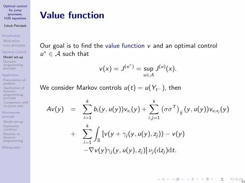
Value function
Our goal is to find the value function v and an optimal controlu∗ ∈ A such that
v(x) = J(u∗) = supu∈A
J(u)(x).
We consider Markov controls u(t) = u(Yt−), then
Av(y) =k∑
i=1
bi (y , u(y))vxi (y) +k∑
i,j=1
(σσT
)ij
(y , u(y))vxixj (y)
+k∑
i=1
∫R
[v(y + γj(y , u(y), zj))− v(y)
−∇v(y)γj(y , u(y), zj)] νj(dzj)dt.
11

Optimal controlfor jump
processes,HJB equations
Jakub Petrasek
Introduction
Motivation
Levy processes
Optimal Control
Model set-up
Dynamicprogrammingprinciple
Application
Formulation ofproblem
Application ofdynamicprogrammingprinciple
Comparison withno-jump case
Maximmumprinciple
Model set-up
Optimalitycondition
Relation todynamicprogramming
Bibliography
Revision
If we start the state process from any t ∈ [0,T − h] it holds
v(Yt) ≥ E
[∫ t+h
t
f (Ys , u(Ys))ds + v(Y(u)t+h)
](2.1)
with equality for u∗ = u. We know that
E tv(Y(u)t+h) = v(Yt) +
∫ t+h
t
A(u)v(Ys)ds
and by substitution into (2.1) we obtain
0 ≥ E
[∫ t+h
t
(f (Ys , u(Ys)) + A(u)v(Ys)
)ds
]
or in differential0 ≥ f (y , u(y)) + A(u)v(y),
for any u and equality holds for u = u∗.12
Optimal controlfor jump
processes,HJB equations
Jakub Petrasek
Introduction
Motivation
Levy processes
Optimal Control
Model set-up
Dynamicprogrammingprinciple
Application
Formulation ofproblem
Application ofdynamicprogrammingprinciple
Comparison withno-jump case
Maximmumprinciple
Model set-up
Optimalitycondition
Relation todynamicprogramming
Bibliography
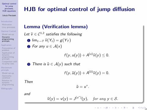
HJB for optimal control of jump diffusion
Lemma (Verification lemma)
Let v ∈ C1,2 satisfies the following
1 limt→T v(Yt) = g(YT )
2 For any u ∈ A(x)
f (y , u(y)) + A(u)v(y) ≤ 0.
3 There is u ∈ A(y) such that
f (y , u(y)) + A(u)v(y) = 0.
Thenu = u∗.
andv(y) = v(y) = J(u∗)(y), for any y ∈ S.
13

Optimal controlfor jump
processes,HJB equations
Jakub Petrasek
Introduction
Motivation
Levy processes
Optimal Control
Model set-up
Dynamicprogrammingprinciple
Application
Formulation ofproblem
Application ofdynamicprogrammingprinciple
Comparison withno-jump case
Maximmumprinciple
Model set-up
Optimalitycondition
Relation todynamicprogramming
Bibliography
Remarks
Verification theorem holds also for random time T however withadditional requirements.
Example
T = inf t > 0,Yt /∈ S
The Hamilton-Jacobi-Bellman equation provides ”only”sufficient condition for an optimum, but not necessary, which isprovided by Pontryagin Maximum principle.
14

Optimal controlfor jump
processes,HJB equations
Jakub Petrasek
Introduction
Motivation
Levy processes
Optimal Control
Model set-up
Dynamicprogrammingprinciple
Application
Formulation ofproblem
Application ofdynamicprogrammingprinciple
Comparison withno-jump case
Maximmumprinciple
Model set-up
Optimalitycondition
Relation todynamicprogramming
Bibliography
Outline
1 IntroductionMotivationLevy processes
2 Optimal ControlModel set-upDynamic programming principle
3 ApplicationFormulation of problemApplication of dynamic programming principleComparison with no-jump case
4 Maximmum principleModel set-upOptimality conditionRelation to dynamic programming
15

Optimal controlfor jump
processes,HJB equations
Jakub Petrasek
Introduction
Motivation
Levy processes
Optimal Control
Model set-up
Dynamicprogrammingprinciple
Application
Formulation ofproblem
Application ofdynamicprogrammingprinciple
Comparison withno-jump case
Maximmumprinciple
Model set-up
Optimalitycondition
Relation todynamicprogramming
Bibliography
Investor’s question
We refer back to the motivation example. An investor puts hismoney into risky St and riskless Bt asset. His portfolio Xt evolves
dXt = ∆tSt−
((α− r)dt + σdWt +
∫ ∞−1
zN(dt,dz)
)+rXtdt−ctXtdt.
and he wants to maximize utility from his consumption
sup(∆t ,Ct)∈A(x)
∫ ∞0
e−βtE U(Ct)dt, (3.1)
Investor knows that his utility is given by the power utility function,i.e.
U(x) =x1−p
1− p, p > 0, p 6= 1,
= log(x), p = 1.
16
Optimal controlfor jump
processes,HJB equations
Jakub Petrasek
Introduction
Motivation
Levy processes
Optimal Control
Model set-up
Dynamicprogrammingprinciple
Application
Formulation ofproblem
Application ofdynamicprogrammingprinciple
Comparison withno-jump case
Maximmumprinciple
Model set-up
Optimalitycondition
Relation todynamicprogramming
Bibliography
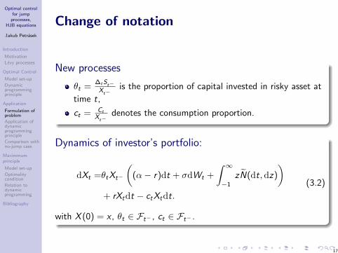
Change of notation
New processes
θt =∆tSt−Xt−
is the proportion of capital invested in risky asset at
time t,
ct = Ct
Xt−denotes the consumption proportion.
Dynamics of investor’s portfolio:
dXt =θtXt−
((α− r)dt + σdWt +
∫ ∞−1
zN(dt,dz)
)+ rXtdt − ctXtdt.
(3.2)
with X (0) = x , θt ∈ Ft− , ct ∈ Ft− .
17

Optimal controlfor jump
processes,HJB equations
Jakub Petrasek
Introduction
Motivation
Levy processes
Optimal Control
Model set-up
Dynamicprogrammingprinciple
Application
Formulation ofproblem
Application ofdynamicprogrammingprinciple
Comparison withno-jump case
Maximmumprinciple
Model set-up
Optimalitycondition
Relation todynamicprogramming
Bibliography
Computation of generator
We would like to apply the verificatin lemma on the controlledprocess Yt = (t,Xt)T , with Y0 = (0, x)T .
Generator of v(Yt)
A(u)v(y) = vt + ((α− r)θ + r − c) xvx +1
2σ2θ2x2vxx
+
∫ ∞−1
(v(t, x + xθz)1−p − v(t, x)− θzvx
)ν(dz).
’Consumption’
f (y , u(y)) = e−βtU(cx).
18

Optimal controlfor jump
processes,HJB equations
Jakub Petrasek
Introduction
Motivation
Levy processes
Optimal Control
Model set-up
Dynamicprogrammingprinciple
Application
Formulation ofproblem
Application ofdynamicprogrammingprinciple
Comparison withno-jump case
Maximmumprinciple
Model set-up
Optimalitycondition
Relation todynamicprogramming
Bibliography
PDE
We guess the form of the value function, v(t, x) = Ke−βtx1−p
A(u)v(y) = Ke−βtx1−p [−β + ((α− r)θ + r − c) (1− p)
− 1
2σ2θ2p(1− p)
+
∫ ∞−1
((1 + θz)1−p − 1− θz(1− p)
)ν(dz)
]= Ke−βtx1−p [−β + (r − c) (1− p) + h(θ)] .
A(u)v(y) + f (y , u(y))
= Ke−βtx1−p
[−β + (r − c)(1− p) + h(θ) +
c1−p
K (1− p)
].(3.3)
19

Optimal controlfor jump
processes,HJB equations
Jakub Petrasek
Introduction
Motivation
Levy processes
Optimal Control
Model set-up
Dynamicprogrammingprinciple
Application
Formulation ofproblem
Application ofdynamicprogrammingprinciple
Comparison withno-jump case
Maximmumprinciple
Model set-up
Optimalitycondition
Relation todynamicprogramming
Bibliography
HJB equations
We apply the verification theorem. We demand
supu∈A
A(u)v(y) + f (y , u(y))
= 0.
We differentiate formula (3.3) with respect to c and θ.
Optimal proportion
0 = Λ(θ) = (α− r)− σ2θp +
∫ ∞−1
(1− (1 + θz)−p
)zν(dz).
Optimal consumption
0 = −(1− p) +c−p
K⇒ c∗ = (K (1− p))−1/p
20

Optimal controlfor jump
processes,HJB equations
Jakub Petrasek
Introduction
Motivation
Levy processes
Optimal Control
Model set-up
Dynamicprogrammingprinciple
Application
Formulation ofproblem
Application ofdynamicprogrammingprinciple
Comparison withno-jump case
Maximmumprinciple
Model set-up
Optimalitycondition
Relation todynamicprogramming
Bibliography
HJB equations
Constant K
Finally we substitute θ∗ and c∗ into equation (3.3) and demandequality to zero
0 = A(u∗)v(y) + f (y , u∗(y))
0 = Ke−βtx1−p [−β + r(1− p) + h(θ∗)
− K−1/p(1− p)−1/p+1 + (K (1− p))−1/p]
= Ke−βtx1−p[−β + r(1− p) + h(θ∗)− p (K (1− p))−1/p
]
⇒ nontrivial solution is
K =1
1− p[β − r(1− p)− h(θ∗)p]−p
.
21

Optimal controlfor jump
processes,HJB equations
Jakub Petrasek
Introduction
Motivation
Levy processes
Optimal Control
Model set-up
Dynamicprogrammingprinciple
Application
Formulation ofproblem
Application ofdynamicprogrammingprinciple
Comparison withno-jump case
Maximmumprinciple
Model set-up
Optimalitycondition
Relation todynamicprogramming
Bibliography
HJB equations
Theorem (Optimal Proportion and Consumption)
Assume the portfolio (3.2) and the objective. Let
Λ(θ∗) = 0
andβ − r(1− p)− h(θ∗) > 0.
Then
θ∗ is the optimal proportion,
c∗ = (K (1− p))−1/p
v(0, x) = Kx1−p is the value function,
where
K =1
1− p[β − r(1− p)− h(θ∗)p]−p
. (3.4)
22
Optimal controlfor jump
processes,HJB equations
Jakub Petrasek
Introduction
Motivation
Levy processes
Optimal Control
Model set-up
Dynamicprogrammingprinciple
Application
Formulation ofproblem
Application ofdynamicprogrammingprinciple
Comparison withno-jump case
Maximmumprinciple
Model set-up
Optimalitycondition
Relation todynamicprogramming
Bibliography
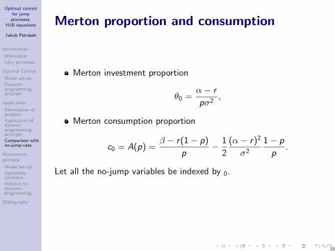
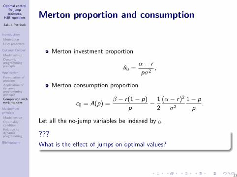
Merton proportion and consumption
Merton investment proportion
θ0 =α− r
pσ2,
Merton consumption proportion
c0 = A(p) =β − r(1− p)
p− 1
2
(α− r)2
σ2
1− p
p.
Let all the no-jump variables be indexed by 0.
???What is the effect of jumps on optimal values?
23
Optimal controlfor jump
processes,HJB equations
Jakub Petrasek
Introduction
Motivation
Levy processes
Optimal Control
Model set-up
Dynamicprogrammingprinciple
Application
Formulation ofproblem
Application ofdynamicprogrammingprinciple
Comparison withno-jump case
Maximmumprinciple
Model set-up
Optimalitycondition
Relation todynamicprogramming
Bibliography
Merton proportion and consumption
Merton investment proportion
θ0 =α− r
pσ2,
Merton consumption proportion
c0 = A(p) =β − r(1− p)
p− 1
2
(α− r)2
σ2
1− p
p.
Let all the no-jump variables be indexed by 0.
???What is the effect of jumps on optimal values?
23

Optimal controlfor jump
processes,HJB equations
Jakub Petrasek
Introduction
Motivation
Levy processes
Optimal Control
Model set-up
Dynamicprogrammingprinciple
Application
Formulation ofproblem
Application ofdynamicprogrammingprinciple
Comparison withno-jump case
Maximmumprinciple
Model set-up
Optimalitycondition
Relation todynamicprogramming
Bibliography
Optimal (jumps included) proportion andconsumption
Optimal proportion θ∗ solves the equation
Λ(θ∗) = (α− r)− σ2θp +
∫ ∞−1
(1− (1 + θz)−p
)zν(dz) = 0.
Optimal consumption
c∗ = (K (1− p))−1/p
for a constant K given by equation (3.4).
24

Optimal controlfor jump
processes,HJB equations
Jakub Petrasek
Introduction
Motivation
Levy processes
Optimal Control
Model set-up
Dynamicprogrammingprinciple
Application
Formulation ofproblem
Application ofdynamicprogrammingprinciple
Comparison withno-jump case
Maximmumprinciple
Model set-up
Optimalitycondition
Relation todynamicprogramming
Bibliography
Function Λ
We know that for Λ0(θ) solves the Merton problem and can see that
1
Λ(0) = α− r ,
Λ(θ) is a decreasing function of θ.
2 Function (1− (1 + θz)−p) z is positive for z ∈ (−1/θ,∞).
We conclude thatΛ(θ) < Λ0(θ).
Corollary
θ∗ ≤ θ0,
v ≤ v0,
c∗ ≤ c0, p > 1,
c∗ ≥ c0, 0 < p < 1.
25

Optimal controlfor jump
processes,HJB equations
Jakub Petrasek
Introduction
Motivation
Levy processes
Optimal Control
Model set-up
Dynamicprogrammingprinciple
Application
Formulation ofproblem
Application ofdynamicprogrammingprinciple
Comparison withno-jump case
Maximmumprinciple
Model set-up
Optimalitycondition
Relation todynamicprogramming
Bibliography
Comparison with Merton cont.
x1 (money units in St)
x2 (money units in Bt)
the Merton line (ν = 0)
risk increasing jumps
(x1 = θ01−θ0x2)
S
S
risk decreasing jumps
26

Optimal controlfor jump
processes,HJB equations
Jakub Petrasek
Introduction
Motivation
Levy processes
Optimal Control
Model set-up
Dynamicprogrammingprinciple
Application
Formulation ofproblem
Application ofdynamicprogrammingprinciple
Comparison withno-jump case
Maximmumprinciple
Model set-up
Optimalitycondition
Relation todynamicprogramming
Bibliography
Approximation of small jumps
Let us suppose that the measure ν has light tails (jumps are small inabsolute value). We can use the taylor expansion
1− (1 + θz)−p = pzθ + o(z2)
and after the substitution into Λ
θ∗ ≈ 1
p
α− r
σ2 +∫∞−1
z2ν(dz),
i.e. for smaller jumps we can approximate Levy process by a
Brownian motion with volatility√σ2 +
∫∞−1
z2ν(dz).
27

Optimal controlfor jump
processes,HJB equations
Jakub Petrasek
Introduction
Motivation
Levy processes
Optimal Control
Model set-up
Dynamicprogrammingprinciple
Application
Formulation ofproblem
Application ofdynamicprogrammingprinciple
Comparison withno-jump case
Maximmumprinciple
Model set-up
Optimalitycondition
Relation todynamicprogramming
Bibliography
Investor’s question II
An investor wants to maximize his utility from the terminal wealth
sup∆t∈A(x)
E U(XT ) (3.5)
Optimal strategy
It is optimal to put constant proportion θ∗ of his money into the riskyasset, same as in the previous.
28

Optimal controlfor jump
processes,HJB equations
Jakub Petrasek
Introduction
Motivation
Levy processes
Optimal Control
Model set-up
Dynamicprogrammingprinciple
Application
Formulation ofproblem
Application ofdynamicprogrammingprinciple
Comparison withno-jump case
Maximmumprinciple
Model set-up
Optimalitycondition
Relation todynamicprogramming
Bibliography
Outline
1 IntroductionMotivationLevy processes
2 Optimal ControlModel set-upDynamic programming principle
3 ApplicationFormulation of problemApplication of dynamic programming principleComparison with no-jump case
4 Maximmum principleModel set-upOptimality conditionRelation to dynamic programming
29

Optimal controlfor jump
processes,HJB equations
Jakub Petrasek
Introduction
Motivation
Levy processes
Optimal Control
Model set-up
Dynamicprogrammingprinciple
Application
Formulation ofproblem
Application ofdynamicprogrammingprinciple
Comparison withno-jump case
Maximmumprinciple
Model set-up
Optimalitycondition
Relation todynamicprogramming
Bibliography
Maximum principle - intro
Alternative approach for solving optimal control.In the deterministic case introduced by Russian mathematicianLev Pontryagin.
State process
Xt = X(u)t with dynamics
dXt = b(t,Xt , ut)dt+σt(t,Xt , ut)dWt+
∫Rγ(t,Xt− , ut− , z)N(dt,dz).
Objective
J(u) = E
[∫ T
0
f (t,Xt , ut)dt + g(XT )
],
for T <∞ deterministic, f continuous, g concave. We want to findan admissible policy u∗ ∈ A such that
J(u∗) = supu∈A
J(u).
30
Optimal controlfor jump
processes,HJB equations
Jakub Petrasek
Introduction
Motivation
Levy processes
Optimal Control
Model set-up
Dynamicprogrammingprinciple
Application
Formulation ofproblem
Application ofdynamicprogrammingprinciple
Comparison withno-jump case
Maximmumprinciple
Model set-up
Optimalitycondition
Relation todynamicprogramming
Bibliography
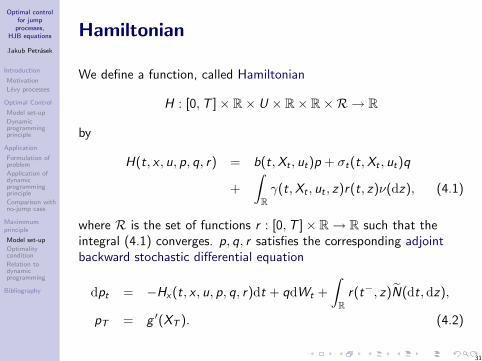
Hamiltonian
We define a function, called Hamiltonian
H : [0,T ]× R× U × R× R×R → R
by
H(t, x , u, p, q, r) = b(t,Xt , ut)p + σt(t,Xt , ut)q
+
∫Rγ(t,Xt , ut , z)r(t, z)ν(dz), (4.1)
where R is the set of functions r : [0,T ]× R→ R such that theintegral (4.1) converges. p, q, r satisfies the corresponding adjointbackward stochastic differential equation
dpt = −Hx(t, x , u, p, q, r)dt + qdWt +
∫R
r(t−, z)N(dt,dz),
pT = g ′(XT ). (4.2)
31

Optimal controlfor jump
processes,HJB equations
Jakub Petrasek
Introduction
Motivation
Levy processes
Optimal Control
Model set-up
Dynamicprogrammingprinciple
Application
Formulation ofproblem
Application ofdynamicprogrammingprinciple
Comparison withno-jump case
Maximmumprinciple
Model set-up
Optimalitycondition
Relation todynamicprogramming
Bibliography
Optimality condition
Let u, u∗ ∈ A and let X ∗t = X(u∗)t , Xt = X
(u)t be the corresponding
state processes. We know that u∗ is optimal if
J(u∗) ≥ J(u), ∀u ∈ A,
and after substitution
J(u∗)−J(u) = E
[∫ T
0
(f (t,X ∗t , u∗t )− f (t,Xt , ut)) dt + g(X ∗T )− g(XT )
]
Assumption
We assume that the integrals in the following derivation are finite.
32
Optimal controlfor jump
processes,HJB equations
Jakub Petrasek
Introduction
Motivation
Levy processes
Optimal Control
Model set-up
Dynamicprogrammingprinciple
Application
Formulation ofproblem
Application ofdynamicprogrammingprinciple
Comparison withno-jump case
Maximmumprinciple
Model set-up
Optimalitycondition
Relation todynamicprogramming
Bibliography
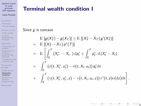
Terminal wealth condition I
Since g is concave
E [g(X ∗T )− g(XT )] ≥ E [(X ∗T − XT ) g ′(X ∗T )]
= E [(X ∗T − XT ) p∗(T )]
= E
[∫ T
0
(X ∗t− − Xt−) dp∗t +
∫ T
0
p∗t−d (X ∗t − Xt)
+
∫ T
0
(σ(t,X ∗t , u∗t )− σ(t,Xt , ut)) q∗t dt
+
∫ T
0
(γ(t,X ∗t , u∗t , z)− γ(t,Xt , ut , z)) r∗(t, z)ν(dz)dt
].
33

Optimal controlfor jump
processes,HJB equations
Jakub Petrasek
Introduction
Motivation
Levy processes
Optimal Control
Model set-up
Dynamicprogrammingprinciple
Application
Formulation ofproblem
Application ofdynamicprogrammingprinciple
Comparison withno-jump case
Maximmumprinciple
Model set-up
Optimalitycondition
Relation todynamicprogramming
Bibliography
Terminal wealth condition II
We substitute into pt and Xt and not rewrite m’gales with zeroexpected value
= E
[∫ T
0
− (X ∗t − Xt) Hx(t,X ∗t , u∗t , p∗t , q∗t , r∗(t, .))dt
+
∫ T
0
p∗t (b(t,X ∗t , u∗t )− b(t,Xt , ut)) dt
+
∫ T
0
(σ(t,X ∗t , u∗t )− σ(t,Xt , ut)) q∗t dt
+
∫ T
0
(γ(t,X ∗t , u∗t , z)− γ(t,Xt , ut , z)) r∗(t, z)ν(dz)dt
].
34

Optimal controlfor jump
processes,HJB equations
Jakub Petrasek
Introduction
Motivation
Levy processes
Optimal Control
Model set-up
Dynamicprogrammingprinciple
Application
Formulation ofproblem
Application ofdynamicprogrammingprinciple
Comparison withno-jump case
Maximmumprinciple
Model set-up
Optimalitycondition
Relation todynamicprogramming
Bibliography
’Consumption’ condition
By the definition of H
E
[∫ T
0
(f (t,X ∗t , u∗t )− f (t,Xt , ut)) dt
]
= E
[∫ T
0
(H(t,X ∗t , u∗t , p∗t , q∗t , r∗(t, .))
−H(t,Xt , ut , p∗t , q∗t , r∗(t, .))) dt
−∫ T
0
p∗t (b(t,X ∗t , u∗t )− b(t,Xt , ut)) dt
−∫ T
0
(σ(t,X ∗t , u∗t )− σ(t,Xt , ut)) q∗t dt
−∫ T
0
(γ(t,X ∗t , u∗t , z)− γ(t,Xt , ut , z)) r∗(t, z)ν(dz)dt
].
35

Optimal controlfor jump
processes,HJB equations
Jakub Petrasek
Introduction
Motivation
Levy processes
Optimal Control
Model set-up
Dynamicprogrammingprinciple
Application
Formulation ofproblem
Application ofdynamicprogrammingprinciple
Comparison withno-jump case
Maximmumprinciple
Model set-up
Optimalitycondition
Relation todynamicprogramming
Bibliography
Terminal wealth + ’Consumption’ condition
J(u∗) − J(u) ≥ E
[∫ T
0
(H(t,X ∗t , u∗t , p∗t , q∗t , r∗(t, .))
−H(t,Xt , ut , p∗t , q∗t , r∗(t, .))) dt
−∫ T
0
(X ∗t − Xt) Hx(t,X ∗t , u∗t , p∗t , q∗t , r∗(t, .))dt
]
and if we find condition such that
J(u∗) − J(u) ≥ 0 (4.3)
we know that u∗ is the optimal control.
36

Optimal controlfor jump
processes,HJB equations
Jakub Petrasek
Introduction
Motivation
Levy processes
Optimal Control
Model set-up
Dynamicprogrammingprinciple
Application
Formulation ofproblem
Application ofdynamicprogrammingprinciple
Comparison withno-jump case
Maximmumprinciple
Model set-up
Optimalitycondition
Relation todynamicprogramming
Bibliography
Theorem
Theorem (Sufficient maximum principle)
Let u∗ ∈ A with corresponding solution X ∗ = X (u∗) and supposethere exists a solution (p∗t , q
∗t , r∗(t, z)) of the corresponding adjoint
equation. Moreover, suppose that
H(t,X ∗t , u∗t , p∗t , q∗t , r∗(t, .)) = sup
u∈UH(t,X ∗t , u, p
∗t , q∗t , r∗(t, .)), t ∈ [0,T ],
andH∗(x) = max
u∈UH(t, x , u, p∗t , q
∗t , r∗(t, .)) (4.4)
exists and is a concave function of x, t ∈ [0,T ] (Arrow condition).Then u∗ is optimal control.
37

Optimal controlfor jump
processes,HJB equations
Jakub Petrasek
Introduction
Motivation
Levy processes
Optimal Control
Model set-up
Dynamicprogrammingprinciple
Application
Formulation ofproblem
Application ofdynamicprogrammingprinciple
Comparison withno-jump case
Maximmumprinciple
Model set-up
Optimalitycondition
Relation todynamicprogramming
Bibliography
Remarks to theorem
Condition (4.4) is guaranteed by concavity of the functionH(t, x , u, p∗t , q
∗t , r∗(t, .)) in (x , u), t ∈ [0,T ].
To finish the proof, denote
h(t, x , u) = H(t, x , u, p∗t , q∗t , r∗(t, .))
andh∗(t, x) = max
u∈Ah(t, x , u)
Optimality condition (4.3) holds if
0 ≤ h∗(t, x∗)− h(t, x , u)− (x∗ − x)h∗′(t, x∗)
≥ h∗(t, x∗)− h∗(t, x)− (x∗ − x)h∗′(t, x∗) ≥ 0.
because h∗ is concave in x for t ∈ [0,T ].
38

Optimal controlfor jump
processes,HJB equations
Jakub Petrasek
Introduction
Motivation
Levy processes
Optimal Control
Model set-up
Dynamicprogrammingprinciple
Application
Formulation ofproblem
Application ofdynamicprogrammingprinciple
Comparison withno-jump case
Maximmumprinciple
Model set-up
Optimalitycondition
Relation todynamicprogramming
Bibliography
Relation to dynamic programming
For the dynamic programming we define criterion
J(u)(s, x) = E
[∫ T−s
0
f (t + s,Xt , ut)dt + g(XT−s)
],
v(s, x) = supu∈A
J(u)(s, x).
Theorem
Assume v ∈ C1,3 and that there exists an optimal control u∗t andcorresponding state process X ∗t for the maximum principle problem.Define
pt = vx(t,X ∗t ),
qt = σ(t,X ∗t , u∗t )vxx(t,X ∗t ),
r(t, z) = vx(t,X ∗t + γ(t,X ∗t , u∗t , z))− vx(t,X ∗t ).
Then pt , qt , r(t, .) solve the adjoint equation (4.2).39

Optimal controlfor jump
processes,HJB equations
Jakub Petrasek
Introduction
Motivation
Levy processes
Optimal Control
Model set-up
Dynamicprogrammingprinciple
Application
Formulation ofproblem
Application ofdynamicprogrammingprinciple
Comparison withno-jump case
Maximmumprinciple
Model set-up
Optimalitycondition
Relation todynamicprogramming
Bibliography
Bibliography
R. Cont and P. Tankov.Financial modelling with jump processes.Chapman & Hall/CRC Financial Mathematics Series., 2004.
K. Janecek.Advanced topics in financial mathematics.Study material, MFF UK, 2008.
B. Øksendal and A. Sulem.Applied stochastic control of jump diffusions. 2nd ed.Universitext. Berlin: Springer., 2007.
40

Optimal controlfor jump
processes,HJB equations
Jakub Petrasek
Introduction
Motivation
Levy processes
Optimal Control
Model set-up
Dynamicprogrammingprinciple
Application
Formulation ofproblem
Application ofdynamicprogrammingprinciple
Comparison withno-jump case
Maximmumprinciple
Model set-up
Optimalitycondition
Relation todynamicprogramming
Bibliography
...
Thank you for attention
41