Dynamic Contracts with Random Monitoring

Andrei Barbos�

Department of Economics, University of South Florida, Tampa, FL.

June 10, 2016

Abstract

In environments where a principal contracts with many agents who each execute numerous

independent tasks, it is often infeasible to evaluate an agent�s performance on all tasks. Incen-

tives under moral hazard are instead provided by monitoring only a subset of randomly selected

tasks. We characterize optimal dynamic contracts implemented with this type of random mon-

itoring technology. We consider a stochastic environment where the agent�s cost of e¤ort varies

over time, and analyze situations where this cost is public or private information. In an optimal

contract, the terms the agent is promised when monitoring reveals compliance are as good as

when no monitoring is performed, and for some cost types are better. These latter types receive

a monitoring reward. We also elicit the dynamics of contract parameters over time. As time

passes and the agent becomes richer, the monitoring reward decreases as the threat of forgoing

the promised stream of future compensation provides su¢ cient incentives for compliance.

JEL Classi�cation: D82, D86

Keywords: Dynamic Contracts; Random Monitoring; Optimal Contracts; Moral Hazard.

�E-mail : andreibarbos@gmail.com; Address : 4202 East Fowler Ave, CMC 206, Tampa, FL 33620-5500; Phone :813-974-6514; Fax : 813-974-6510; Website : https://sites.google.com/site/andreibarbos/

1 Introduction

Existing literature on dynamic contracting under moral hazard examines situations where in every

period of the game, the principal observes a signal correlated with the action chosen by the agent in

that period.1 In certain contractual environments, particularly those where the principal interacts

with a large number of agents who each performs numerous independent tasks over the lifetime of

the contract, it is infeasible or too costly to make observations about an agent�s performance on all

tasks that he is assigned. Instead, in many such situations, the agent is provided with incentives

by evaluating his performance only on a randomly generated subset of these tasks. In this paper

we study optimal dynamic contracting under moral hazard when contracts are implemented with

this type of random monitoring technology. Speci�cally, we consider an in�nitely repeated game in

which in every period the agent chooses a payo¤ relevant action (an e¤ort level) and the principal

employs a monitoring instrument which, with some non-degenerate probability, reveals the precise

action chosen by the agent, but otherwise reveals no informative signal of it.

Optimal contracts with random monitoring are investigated in a static framework in Barbos

(2016). An implicit assumption underlying static modeling of contractual environments is that

a contract is signed and executed for every action that the agent performs. However, in many

real-world situations where random monitoring is employed, the sort of physical constraints or cost

structures that preclude monitoring the performance of an agent on all tasks are also likely to

preclude contracting of each task. Instead, contracts are usually signed at the outset of a long-term

relationship (for instance, at the time when a worker is hired) and then the agent is assigned a

series of tasks over the period of the contract. In these situations, the principal can design contracts

that incentivize the agent to expend resources on a task by means of both current period transfers

and promises about future compensation. The goal of this paper is to derive properties of optimal

contracts implemented with random monitoring in such dynamic environments.

1This signal may take the form of a noisy observation of the agent�s action, but may also consist of an aggregateor average level of the agent�s actions.

2

The sequential nature of interaction speci�c to typical real-world dynamic contractual relation-

ships makes the assignment of tasks be done with a delay after the contract is signed. Therefore,

the agent often learns the precise cost of executing a task only at the time when the task is assigned.

We capture this feature in our model by assuming that the marginal cost of the resources (e¤ort,

time, etc.) spent by the agent in executing the current period action depends on a state of nature,

referred to as his cost type, which evolves stochastically over time. The realizations of the cost

type in di¤erent periods are independent and identically distributed. In the main speci�cation of

the model we consider the case where the type is publicly observed in every period.

An example of a situation captured by our model is that of a service provider whose workers

execute a large number of tasks.2 Such a worker, when dealing with a customer, chooses the level

of customer satisfaction to deliver, interpreted as his action, while the variable complexity of the

issue being addressed determines the cost of delivering that level. Monitoring is performed by the

employer through feedback obtained from a random subset of customers served by the worker.3

In the recursive formulation of contracts that we employ in our analysis, the agent starts every

period with a continuation value that captures the present value of the stream of future expected

utilities promised to him. Accounting for this value, the contract speci�es a recommended action

for each possible realization of the agent�s cost type, and a current period transfer and next period

continuation value for each contingency that may emerge during the period of play.

A salient feature of contract design under random monitoring is that incentives to exert e¤ort

can only be provided with the contract variables speci�ed for contingencies where monitoring is

executed. These variables must thus be set su¢ ciently high. On the other hand, when the agent is

risk averse, e¢ ciency requires minimizing the variance in the sets of current period transfers and

next period continuation values. These two goals are misalligned and therefore a key aspect of the

analysis of contracts with random monitoring consists in eliciting the solution to this trade-o¤. A

2This example is borrowed from Barbos (2016).3For instance, most car dealerships request feedback from the customers of their service center by asking them to

complete a survey about general satisfaction and about more speci�c aspects, such as the quality of service performedby the manager, technician, billing department, etc. The imperfect response rate makes such monitoring random.

3

second trade-o¤, speci�c to problems of dynamic contracting, emerges from the option to deliver

utility to the agent through both current and future transfers. The shape of the optimal contracts

in this environment is determined by the solution to these two trade-o¤s and their interplay. Specif-

ically, the �rst trade-o¤ is solved by promising the agent a monitoring reward that comes in the

form of a better contractual terms to a complying agent when monitoring is performed than when

it is not. The second trade-o¤ implies that this reward is decreasing in time as the agent gets richer.

E¢ ciency dictates that the current period transfers and the next period continuation values be

constant across contingencies where they do not play a role in implementing the current period

action. These contingencies are those where the recommended e¤ort level is zero or where monitor-

ing is not performed. Additionally, to minimize the intertemporal variance in the agent�s income,

the corresponding next period continuation values are set equal to the current period continuation

value. The contract parameters speci�ed for contingencies where a positive e¤ort level is recom-

mended and monitoring reveals compliance are set at the same common levels whenever these levels

are su¢ cient to provide the agent with incentives to exert e¤ort. For the remaining contingencies,

incentive provision requires that these contract parameters be set at higher levels, while e¢ ciency

that the corresponding incentive constraints bind. Complying agents of certain cost types are thus

promised a monitoring reward that comes in the form of a higher next period continuation value

and current period transfer than the corresponding contract parameters with no monitoring.

A consequence of the optimal choice of next period continuation value is that as the agent�s

type �uctuates over time, this value stays constant at the end of periods with no monitoring and of

periods where the incentive constraint for exerting e¤ort does not bind, and increases at the end of

the remaining periods.4 The current period transfers are set equal to zero when the continuation

value is small since the marginal cost of delivering utility to the agent through promises of future

transfers is lower. When positive, the current period transfers increase as the continuation value

increases over time. The monitoring reward is thus o¤ered to complying agents at the beginning

4Unlike dynamic contracting models that assume standard noisy monitoring, where low realizations of the infor-mative signal may decrease the continuation value in the next period, in our model, this value is non-decreasing.

4

of the contractual relationship when the low levels of the continuation value and current period

transfer imply that the incentive constraint for e¤ort provision binds. As the continuation value

increases over time and the contract terms for contingencies where incentive provision is unnecessary

improve, the size of this reward decreases and at some point is eliminated.

We also examine the dynamics of the e¤ort level implemented in an optimal contract. At the

beginning of the contractual relationship, when the incentive constraint for e¤ort binds, this e¤ort

level is independent of the continuation value and is a function solely on the agent�s e¢ ciency. As

the continuation value increases over time, the marginal cost of compensating the agent for e¤ort

increases. At some point, the e¤ort level required from each type starts decreasing between periods

in which the continuation value increases and fewer types are required to exert e¤ort. When this

value is su¢ ciently high, compensating the agent for e¤ort under any state of the world becomes

too costly. At that time, the agent is retired and thereafter made a constant transfer each period

which maintains the continuation value at the same level for perpetuity.5

As an extension, we also study a model where the state of the world that determines the agent�s

random cost type is private information to the agent. As in the static model from Barbos (2016),

we consider the case where the agent can communicate this state through a non-veri�able message

and thus the principal can adjust current period transfers and next period continuation values as a

function of this message. Our analysis elicits several qualitatitive features of the optimal contracts

in this framework which are distinct from those under pure moral hazard.

First, under adverse selection the monitoring reward decreases in the cost e¢ ciency of the

agent, with the less e¢ cient types being promised the same terms with monitoring as without when

complying. Second, adverse selection induces ine¢ ciency in the choice of implemented e¤ort level.

This level maximizes each type�s virtual surplus that accounts for the information rents the agent

has to be paid for his private type information, and is lower than the e¤ort level from a situation

with pure moral hazard that instead maximizes an intuitive notion of social surplus. Finally, when

5 In models with noisy monitoring where the continuation value may decrease, retirement also occurs when thisvalue reaches a lower bound (for instance, Spear and Wang (2005), Sannikov (2008)).

5

the agent is risk-neutral, unlike a situation with pure moral hazard where the �rst-best outcome can

always be implemented, under adverse selection, this is possible only under an additional condition

which ensures that the limited liability constraint of the agent is not violated. These �ndings show

that some key qualitative features of the optimal contracts uncovered in the static version of the

model with moral hazard and adverse selection extend to a dynamic environment.

This paper belongs to the vast literature of dynamic contracting under moral hazard. Some of

the early seminal papers from this literature are Radner (1981), who examined a situation where

the publicly observed period outcome depends on the agent�s action and some state of the world

which are both privately observed by the agent, Townsend (1982), which studied dynamic contracts

under adverse selection, Rubinstein and Yaari (1983), which elicited the role of temporal incentives

in mitigating the ine¢ ciencies induced by moral hazard in repeated relationships, and Rogerson

(1985), which showed that in a repeated moral hazard model where the agent can neither borrow

nor save, the inverse marginal utility of consumption evolves as a martingale. Spear and Srivastava

(1987) were the �rst to employ recursive methods for solving dynamic contracts. Some of the more

recent contributions to this literature are Sannikov (2008), which studies contracting under moral

hazard in a continuous time model, Biais, Mariotti, Rochet and Villeneuve (2010), which considers

a model where the agent exerts e¤ort to preempt large losses and his limited liability hinders risk

sharing, and Kovrijnykh (2013) which studies the case where the principal has a limited ability to

commit to enforce a contract. Our paper makes a contribution to this literature by considering

situations where contracts are implemented with a random monitoring technology.6 While some of

the insights that it uncovers are familiar from earlier papers, other �ndings are speci�c due to the

distinct set of contingencies on which contracts with random monitoring can be designed.

Section 2 introduces the model and some preliminaries, including the analysis of the full-

information benchmark. Section 3 presents the analysis of the pure moral hazard model, while

section 4 presents the analysis of the model with moral hazard and adverse selection. Section 5

6Fraser (2012) considers a two-period contracting problem under random monitoring in the context of agri-environmental policy. He analyzes numerically the e¤ect of various model parameters on the incentives of the agentto deviate from the prescribed policy and illustrates the potential use by the principal of inter-temporal incentives.

6

concludes. Most proofs are relegated to the appendix.

2 Framework and Preliminaries

The Model There are two risk-neutral players, a principal (P) and an agent (A), who interact

repeatedly over an in�nite number of time periods and evaluate future streams of utility with a

common discount factor � 2 (0; 1). P owns a �rm and can o¤er an employment contract to A,

which A may accept or reject. When A exerts e¤ort e in a given period, he produces output with

value y(e), which is entirely appropriated by P through his �rm. We assume y(0) = 0, y0 (�) > 0,

y00 (�) � 0, and that and y is bounded on R+. If A receives a wage � and exerts e¤ort e in a

given period, his current period utility is u(�) � c(s; e). The function u : R ! R captures A�s

preferences over monetary transfers. We denote the corresponding inverse utility function by h(u)

and throughout the analysis substitute the current period induced utilities u � u(�) as choice

variables in the optimal contract problem in place of wages. To distinguish u from the total utility

experienced by A in a period, which also accounts for the cost of e¤ort, we will refer in the following

to u as the wage-utility. We assume h0 (�) > 0 and h00 (�) � 0, and normalize h(0) = 0. c(s; e) is

the cost for A of exerting e¤ort e, where (i) s is a random variable, (ii) c (�; �) is a function with

c (s; 0) = 0, ce > 0, cee > 0, cs > 0 and ces > 0, for all s 2 [s; s] and e � 0. The realizations of

the random variable s are independent over time and distributed with density function f(�) on an

interval [s; s] � R. The functions y, h and c are twice continuously di¤erentiable.

We examine models with two speci�cations of the information structure. In a pure moral hazard

model, the realization of the state s is public information in every period. As an extension, we also

analyze a model with moral hazard and adverse selection in which the state s is observed only by

A; A can non-veri�ably communicate the state and the corresponding message is contractible.

P has at his disposal an imprecise monitoring technology which allows publicly observing the

e¤ort exerted by A in a given period with some probability r 2 (0; 1). With probability 1 � r, P

does not observe either e or any informative signal about it. P incurs no additional cost when he

7

observes the e¤ort exerted by A. A does not know at the time when he chooses the level of e¤ort

to exert in a given period whether or not P will observe this level.

Once A accepts a contract o¤ered by P, this contract is binding for the two players. A�s outside

option at the beginning of the employment relationship is normalized to have an expected present

value equal to zero. We assume limited liability for the agent meaning that the wage that he

receives in any period and under any contingency must be non-negative.

Recursive Approach As in other papers, we analyze this game by looking for the set of Pareto

optimal subgame perfect equilibria.7 Finding the Pareto equilibria requires solving an optimization

problem where the expected equilibrium payo¤ of one player is maximized subject to delivering at

least a certain expected equilibrium payo¤ to the other player. The standard approach to solving

this problem in the context of dynamic games, introduced by Spear and Srivastava (1987), is to

rewrite it in a recursive form with the current promised expected discounted value of future payo¤s

to one player as the state variable, and the contingent continuation values to that player, as well

as the period actions by both players, as the control variables.

Contracts and Timing Since the discussion of how to transform a sequential optimization

problem into its recursive representation is standard in the literature, we forgo including it here

and instead assume directly that P o¤ers recursive contracts. These contracts specify for any

continuation value w at the beginning of a period and for each state s 2 [s; s], publicly observed or

communicated by A, a set fes; us(e); uns ; ws(e); wns g, where (i) es is the level of e¤ort recommended

to be exerted in the current period; (ii) us(e) is the wage-utility delivered to A by the current

period transfer promised for the case when monitoring is performed and the observed e¤ort level is

e; (iii) uns is the wage-utility delivered to A by the current period transfer when monitoring is not

performed; (iv) ws(e) is A�s continuation value at the beginning of the next period if monitoring

7As a reminder, this is the set of subgame perfect equilibria with expected discounted payo¤s for the two playerssuch that there exist no other subgame perfect equilibrium in which both players enjoy weakly higher payo¤s and atleast one player a strictly higher payo¤.

8

is performed and the observed e¤ort is e; (v) wns is A�s continuation value at the beginning of the

next period when monitoring is not performed. As standard in the literature, we allow P to o¤er

probability mixtures over continuation values in any given contingency.8

We make now two straightforward observations that allow us to reduce the set of contracts that

we consider; the formal arguments supporting these observations in a static framework from Barbos

(2016) extend immediately to this dynamic setting. Thus, note �rst that in any optimal contract,

it must be that us(e) = 0 and ws(e) = 0 for all e 6= es, as this o¤ers A the strongest incentives to

choose e¤ort level es. Since e¤ort is costly, A will then either exert e¤ort es or 0. Employing these

remarks, in the following, we denote by us and ws the current period wage-utility and continuation

value, respectively, when monitoring reveals that A exerted the recommended e¤ort level es.

With these observations, the timing of the contract in any period can be summarized as follows.

(i) At the beginning of the period, A is endowed with a continuation value w that may be the

outcome of a lottery; in the �rst period, w equals 0. P presents a set of contract variables

fes; us; uns ; ws; wns gs2[s;s], with an expected value to A of at least w when A complies with the

e¤ort recommendation for the state of nature to be realized in that period.

(ii) The random state s is realized. In the pure moral hazard model, s is publicly observed. In

the model with moral hazard and adverse selection, s is observed only by A. In the latter

case, A non-veri�ably communicates it to P.

(iii) A exerts e¤ort. Simultaneously, nature determines if monitoring is performed or not.

(iv) If monitoring is performed and the e¤ort observed equals es, A is delivered a wage-utility us

in the current period and is promised a continuation value for the next period ws; if the e¤ort

is di¤erent than es the wage-utility and continuation value are set at 0. If monitoring is not

performed, the wage-utility is uns and the continuation value is wns .

8This will imply that the value function in the recursive optimization problem is concave. Note that it is assumedthat P can o¤er lotteries over continuation values in the next period (i.e., over future streams of utility) and not overcurrent period wage-utilities. In fact, P has no reason to o¤er the latter, as it would require paying a risk premium.

9

The Full-Information Benchmark The �rst-best outcome in this framework corresponds to

a situation with full information. If P observes both A�s type and the e¤ort exerted, monitoring

plays no role. P thus o¤ers a contract�e0s(t); u

0s(t)

s2[s;s], where e

0s(t) is the e¤ort required from

type s in period t, and u0s(t) is the wage-utility delivered to type s at the end of period t.

The next proposition presents the intuitive conditions de�ning the corresponding optimal con-

tract when A is strictly risk averse, i.e., when h00 > 0. Since its proof employs concepts and results

that are introduced in more generality in the proofs of the results from the model with unobserved

e¤ort, the proof is included in appendix A1 after the proofs of the results from section 3.

Proposition 1 Assume A is strictly risk averse over monetary transfers. The full information

optimal contract is stationary over time with u0s(t) = u0 > 0 and e0s(t) = e

0s for all s 2 [s; s], where

y0�e0s�� h0(u0)ce(s; e0s) � 0, and = 0 if e0s > 0 (1)

It is straightforward to show that if the agent is risk neutral, then in the optimal contract,

the e¤ort pro�le satis�es ce(s; e0s) = y0�e0s�for all s 2 [s; s] with e0s > 0, while any nonnegative

wage-utility pro�le�u0ss2[s;s] satisfying

R ss u

0sf(s)ds =

R ss ce(s; e

0s)f(s)ds is optimal.

3 The Pure Moral Hazard Model

Clearly, an optimal contract which induces strictly positive e¤ort for some type s in a given period,

must also induce strictly positive e¤ort for all types that are more e¢ cient than s.9 Thus, for any

continuation value w, there exists some value bs 2 [s; s], such that, optimally, es > 0 a.e. s 2 [s; bs),9 If types are distributed uniformly on [s; s], a contract that does not satisfy this property can be improved by

shifting required e¤ort from a less e¢ cient type to the more e¢ cient one with zero e¤ort while also swapping theremaining contract variables between the two types. All incentive constraints will be satis�ed by the new contract,but A will experience a higher ex-ante utility since the cost of exerting the e¤ort is lower. P can then appropriateat least partially this surplus by reducing the wages of the e¢ cient types who are now working and whose incentiveconstraints are loose. The same type of adjustment can be performed when types are not uniformly distributed, butin that case, one needs to shift e¤ort between two sets of types of equal measure.

10

and es = 0 a.e. s 2 [bs; s]. Employing this observation, it follows that the recursive form of the

optimal contract problem is

V (w) = maxbs;fes;ws;wns ;us;uns gs2[s;s]Z s

sfy (es) + r [�V (ws)� h (us)] + (1� r) [�V (wns )� h (uns )]g f(s)ds

(2)

subject to: r (�ws + us)� c (s; es) � 0, for all s 2 [s; bs) (ICE)Z s

s[r (�ws + us) + (1� r) (�wns + uns )� c (s; es)] f(s)ds � w (PKC)

es � 0, ws � 0, wns � 0, us � 0, uns � 0, for all s 2 [s; s]; es = 0, for all s 2 [bs; s] (3)

Condition (ICE) (Incentive Compatibility for E¤ort) ensures that A exerts the recommended e¤ort

level in states s 2 [s; bs). Condition (PKC) (Promise-Keeping Constraint) requires that the expectedvalue of A�s future stream of utilities, evaluated at the beginning of the current period, is at least

w when accounting for the probability distribution of the current period wage-utility, e¤ort, and

next period continuation value. The constraints in (3) are consequences of A�s limited liability and

of the de�nition of bs. The existence of a solution to problem (2)-(3) is studied in appendix A2.

To reduce the complexity of the notation in the text of the above problem and in the ensuing

analysis, we forgo specifying explicitly throughout that the various payo¤s may be random because

P may o¤er lotteries over continuation values. Instead, with a slight abuse of notation, we write

the expected value of a lottery over continuation values in place of the corresponding lottery.10

We examine �rst the case where A is strictly risk averse over monetary transfers, implying that

h is strictly convex. The next lemma elicits some key properties of the value function V in any

solution to (2)-(3). The proofs of all results from this section are presented in appendix A1.

Lemma 2 (Value Function) The value function V is strictly decreasing and concave in w.

10More precisely, this is the case when writing A�s payo¤s. For P�s payo¤s, when P o¤ers a lottery (w0; p;w00; 1�p),with expected value w, we can write V (w) instead of pV (w0) + (1� p)V (w00) because the two values are equal as Vis linear on (w0; w00). This is because P o¤ers lotteries precisely when otherwise V would be convex on (w0; w00) andthus P increases his expected payo¤ with a lottery over (w0; w00) that linearizes the value function on that interval.

11

The fact that V is strictly decreasing in w is essentially equivalent to (PKC) always binding

at the optimal solution. To understand the intuition for this fact, note that if (PKC) does not

bind then (ICE) must bind for all types s 2 [s; bs) since otherwise es could be increased so as tostrictly increase the value of the objective function. Employing this insight, (PKC) can be rewritten

as (1� r)R ss (�w

ns + u

ns ) f(s)ds > w. It follows then that the contract delivers A more than the

promised utility w even though all surplus is delivered through the contract variables wns and uns ,

which do not play a role in implementing e¤ort but only in minimizing the risk premium that P

needs to pay. This cannot be optimal because slightly reducing these variables would increase the

value of the contract. (PKC) must thus bind and therefore V is strictly decreasing in w. The proof

of the lemma accounts for the fact that we do not know apriori that V is strictly decreasing, so

the above argument may not necessarily lead to a contradiction if uns = 0, but wns > 0. Therefore,

the argument in the appendix proceeds by showing �rst that V is strictly decreasing in w, from

which it follows that (PKC) must bind. On the other hand, the concavity of the value function is

a consequence of the fact that P can o¤er lotteries over the continuation values.

The properties of the optimal solution that are identi�ed below hold on all [s; s], but a set

of measure zero. To avoid specifying this each time, in the following we restrict attention to the

solution�bs; fes; ws; wns ; us; uns gs2[s;s]� to (2)-(3) in which the properties we identify hold everywhere.

We will characterize the optimal contract in a series of propositions. To this goal, denote �rst

by V 0�(w), V0+(w) and @V (w) the left derivative, the right derivative, and the superdi¤erential of

the function V at w. Let also w � inf�w��V 0+(w) = �h0(0).

Proposition 3 (Optimal Continuation Values) The optimal choice of continuation values sat-

is�es: (i) wns = w for all s 2 [s; s]; (ii) ws � w for all s 2 [s; s]; (iii) ws = w for all s 2 [s; bs) forwhich (ICE) does not bind, and for all s 2 [bs; s].

Since V is concave, it is optimal to set the continuation value in the next period as close to w as

possible. In particular, this continuation value is set at w for all contingencies where it plays no role

12

in the incentive scheme that implements the current period e¤ort, i.e., for contingencies where no

monitoring is performed (thus, wns = w for all s) or where the recommended e¤ort is 0 (thus, ws = w

for s 2 [bs; s]). On the other hand, the choice of next period continuation values for contingencieswhere positive e¤ort is implemented and monitoring is performed is the solution to the trade-o¤

between e¢ ciency and incentive provision. When the incentive constraint (ICE) does not bind if

ws were set at w, this trade-o¤ can be solved with no loss of e¢ ciency. Otherwise, ws must be

set above w to provide su¢ cient incentives for the agent to follow the e¤ort recommendation (as

lemma 6 below elicits, for any s, this occurs for the lower values of w). To minimize the variance

in the set of continuation values in such situations, ws is set at the lowest level which satis�es the

incentive constraint, and thus (ICE) binds. It is never optimal to set ws below w as this induces

an e¢ ciency loss with no gain in the incentive scheme.

Proposition 4 (Optimal Wage-Utilities) There exists uz � 0 such that the optimal choice of

current period wage-utilities satis�es: (i) uns = uz for all s 2 [s; s]; (ii) us � uz for all s 2 [s; s];

(iii) us = uz for all s 2 [s; bs) for which (ICE) does not bind, and for all s 2 [bs; s]; (iv) uz = 0

whenever w � w; (v) for any s 2 [s; bs), us = 0 whenever ws � w.By the same logic as that underlying proposition 3, since A is risk averse, the contract minimizes

A�s wage risk, and thus the current period wage-utilities are equal to some value uz across all

contingencies where they are not employed in incentive provision. In the remaining contingencies,

the wage-utility is at least as high as uz; otherwise, it could be increased while at the same time

decreasing uz to reduce the wage risk on A while still satisfying the two constraints. In a dynamic

environment, at the beginning of every period, P can exploit the richness of the contract to provide

incentives to A through both current period transfers and promises about future transfers. Parts

(iv) and (v) of the proposition elicit a qualitative property of the optimal contract which is familiar

from other dynamic principal-agent models.11 Speci�cally, the current period wage-utilities are

optimally set at 0 when the continuation value in the next period is low enough, i.e., given the

11See, for instance, Sannikov (2008) or Kovrijnykh (2013).

13

concavity of the value function V , when the marginal cost of providing incentives through promises

of future transfers is low. The continuation value must reach w with probability one after any

history of play since otherwise A never would consumes in that subgame; thus, w is �nite.

Propositions 3 and 4 imply that if (ICE) binds for type s when the current continuation value is

w, the expected lifetime utility delivered to a complying agent of type s when monitored is higher

by an amount (�ws + us)� (�w + uz) > 0 than when not monitored. This di¤erence constitutes a

monitoring reward that the complying agent receives. As also elicited by Barbos (2016), this implies

that when random monitoring is employed for incentive provision in a contractual relationship, it

is optimal to not only to punish the agent for deviations from the prescribed e¤ort level, but also

to reward him when monitoring is executed and compliance is observed. This reward may come in

the form of higher current period transfers and/or of promises about higher future compensation.

Contracts that only punish observed deviations, but otherwise o¤er the same terms whether or not

monitoring is executed, may not implement the desired level of e¤ort in an optimal way.

Proposition 5 (Optimal E¤ort) (i) The optimal choice of e¤ort satis�es

0 2 y0(es) + ce (s; es) @V (ws) , for s 2 [s; bs) (4)

(ii) For any w, es is strictly decreasing in s for all s 2 [s; bs).Proposition 5 elicits properties of the optimal e¤ort schedule. Condition (4) states the stan-

dard equality between the marginal bene�t of implementing additional e¤ort in some state s,

y0(es), and the marginal cost of compensating A for that e¤ort, which is an element in the set

ce (s; es) [�@V (ws)], and when V is di¤erentiable at ws equals �ce (s; es)V 0 (ws). As expected, P

implements lower e¤ort levels for less e¢ cient types. As we argue in the appendix, the monotonic-

ities of ws and us with respect to s are generically ambiguous because, as s increases, the higher

marginal cost of e¤ort may be o¤set by the lower e¤ort level that is recommended. The size of the

monitoring reward is thus generically non-monotonic with respect to the e¢ ciency of the agent.

14

Lemma 6 For any s, there exists a value ews, such that (ICE) binds if and only if w � ews.Moreover, whenever w � ews, it is optimal to set ws = ews.

The threshold ews is the minimum level at which the current period continuation value w providessu¢ cient incentives for e¤ort to type s when setting the contract parameter ws equal to w. Since

the concavity of V requires the next period continuation value be as close to the current value as

possible, ews is precisely the level at which ws is set whenever w is not su¢ ciently high and (ICE)binds.12 An implication of lemma 6 is that A receives the monitoring reward for low values of

w. When the agent is rich enough, the threat of possibly losing the value of the promised future

compensation is su¢ ciently strong to induce compliance with the e¤ort recommendation.

Proposition 7 describes the dynamics of the contract parameters over time.

Proposition 7 (Dynamics of the Contract Parameters) The continuation value weakly in-

creases over time. Whenever it increases between two periods to a new level w, the contract para-

meters have the following dynamics: (i) ws stays constant at ews if w � ews, and strictly increasesif w > ews; (ii) wns strictly increases; (iii) us stays constant if w � ews, and increases if w > ews;(iv) uns increases; (v) es stays constant if w � ews, and decreases if w > ews; (vi) bs decreases.

The dynamics of the current period continuation value are an immediate consequence of proposi-

tion 3 and lemma 6. By proposition 3, as the state �uctuates from period to period, the continuation

value increases at the end of periods with monitoring and realizations of s such that ews > w, andstays constant at the end of all other periods. This value never decreases from period to period.

To understand parts (i)-(iv), consider any pair of consecutive periods such that the continuation

value at the beginning of the second period equals w with w strictly higher than the level of the

continuation value at the beginning of the earlier of the two periods. By lemma 6, when w satis�es

w � ews, it is optimal to set ws = ews, implying that ws stays constant between the two periods.12Generically, ews is non-monotonic in s and may take values below or above w.

15

When w > ews, then ws = w and therefore ws increases to w either from ews or from the level of the

continuation value in the �rst period. The fact that wns increases between the two periods follows

from the fact that wns is always set equal to the current level of the continuation value. Since

the marginal cost of implementing e¤ort through promises about current and future transfers, i.e.,

though us and ws, respectively, should optimally be equal whenever us > 0, the dynamics of us are

identical to those of ws. Similarly, the dynamics of uns are identical to those of wns when u

ns > 0.

As part (v) states, for low values of w where constraint (ICE) binds, es is independent of w. To

understand this, recall that the recommended e¤ort level is determined by the trade-o¤ between

the marginal product and the marginal cost for P of implementing e¤ort. By proposition 5(i), the

marginal cost is a function of the contract parameter ws. Therefore, since whenever w � ews, wsis set equal to ews, implying that ws is independent of the current continuation value w, the e¤ortlevel es is also independent of w. At the beginning of a contractual relationship, when the promised

continuation value is low, P implements thus an e¤ort level that is solely a function of the state

s. As time passes and the continuation value satis�es w > ews for some state s, the e¤ort requiredfrom the agent of type s 2 [s; bs) starts decreasing since the higher value of w increases the cost ofcompensating marginal e¤ort. Moreover, by the same intuition, as w increases, A is required to

exert e¤ort under fewer realizations of the state variable s and thus bs decreases, as stated by (vi).An implication of the dynamics of these contract parameters is that the size of the monitor-

ing reward promised to an agent of type s, (�ws + us) � (�w + uz), decreases over time as the

continuation value increases, and disappears when the continuation value reaches a level above ews.The following proposition identi�es the condition that de�nes the continuation value at which

the agent is retired, meaning that he is no longer required to exert e¤ort under any realization of

the state. To this aim, denote by w � infnw���V (w) = � 1

1��h((1� �)w)o.

Proposition 8 (Retirement Condition) (i) For any w, V (w) � � 11��h((1� �)w), with equal-

ity if es = 0 for all s 2 [s; s]; (ii) For any w � w, es = 0 for all s 2 [s; s].

16

When the continuation value reaches a value w � w, the agent is already rich enough that

compensating him for e¤ort becomes too costly. The agent is then retired and delivered utility

equal to (1� �)w every period, maintaining the continuation value at the beginning of every period

constant at w. The resulting value of the contract to the principal is � 11��h((1� �)w).

13 Spear

and Wang (2005) and Sannikov (2008) identify a similar result in discrete-time and continuous-

time, respectively, contracting problems under moral hazard. Since these papers assume a standard

noisy monitoring technology, a sequence of low realizations of the output, as informative signals

of the agent�s e¤ort, may lead the continuation value to reach a lower bound at which retirement

is necessary since the incentivizing is not longer possible as the agent is too poor to be able to be

punished if further low realizations of the output were to occur. Since in our model the continuation

value is optimally non-decreasing, this second type of retirement condition does not emerge.

Proposition 9 (Monitoring Intensity) V (w) is increasing in r for all w and all r.

The value of the contract is increasing in the intensity of monitoring. When r increases, P can

rely less on the power of incentives and o¤er a smoother set of contract parameters. This reduces

the dispersion in the set of possible continuation values and in the set of current period transfers,

increasing the value of the contract since V is concave and A is risk averse. On the other hand, a

higher value of r also increases the probability that A is paid the monitoring reward; this has an

e¤ect of reducing the value of the contract. Proposition 9 shows that the �rst e¤ect dominates.

The closing result of the section states that the �rst-best value of a contract can be attained un-

der moral hazard if A is risk neutral. The corresponding contract satis�es the incentive constraints

solely through promises about the current period transfers for contingencies where monitoring is

performed and A is required to exert positive e¤ort. The remaining transfers as well as the contin-

uation values are always set to 0.

13As shown in the appendix, the functions V (w) and � 11��h((1� �)w) also exhibit the so-called smooth pasting

property, meaning that their �rst-order derivatives are equal at w (V is shown to be di¤erentiable at w).

17

Proposition 10 (Risk Neutral Agent) If A is risk neutral, the value of the optimal contract

under moral hazard equals the value of the optimal contract under full information.

Proof. Let ws = 0, wns = 0 and uns = 0 for all s 2 [s; s]. Also, let es = e0s and us =1r c(s; e

0s) for

all s 2 [s; s]. If A is risk neutral, these contract parameters satisfy all the constraints in problem

(2)-(3) for w = 0, therefore implementing the �rst-best outcome. Since A�s outside option has value

0, A starts the �rst period of the game with w = 0, and therefore the �rst-best outcome can be

implemented in that period. Moreover, by the speci�cation of the continuation values, A will start

the next period with w = 0. By induction, this contract implements the �rst-best outcome in all

periods. Since the cost to P is equal to that under full information, this contract is optimal as its

value attains the upper bound, i.e., the value of the optimal contract under full information. �

4 Extension: Model with Moral Hazard and Adverse Selection

As an extension of the pure moral hazard model analyzed in the previous section, we also examine

a situation where the state of the world in any period of the game is observed privately by the

agent and can be communicated to the principal through a non-verifyable message. The principal

can o¤er contracts with parameters that are functions of this message. For simplicity, we assume

in this section that it is optimal to implement strictly positive e¤ort for all types. The additional

insights uncovered by the analysis of a more general model that does not employ this assumption

are similar to those derived in the static case examined in Barbos (2016).

In designing the optimal contract under moral hazard and adverse selection, P has to preempt

two possible types of deviations by A. First, P needs to ensure that an agent of type s does not

communicate a message es 6= s and then exerts the e¤ort recommended for es. Second, P needs toensure that A does not communicate some message es and then exerts no e¤ort.14 The recursive14We employed again here our observation that P promises a wage equal to 0 for situations where monitoring

reveals an e¤ort level di¤erent than the one speci�ed for the state of the world that A previously communicated.

18

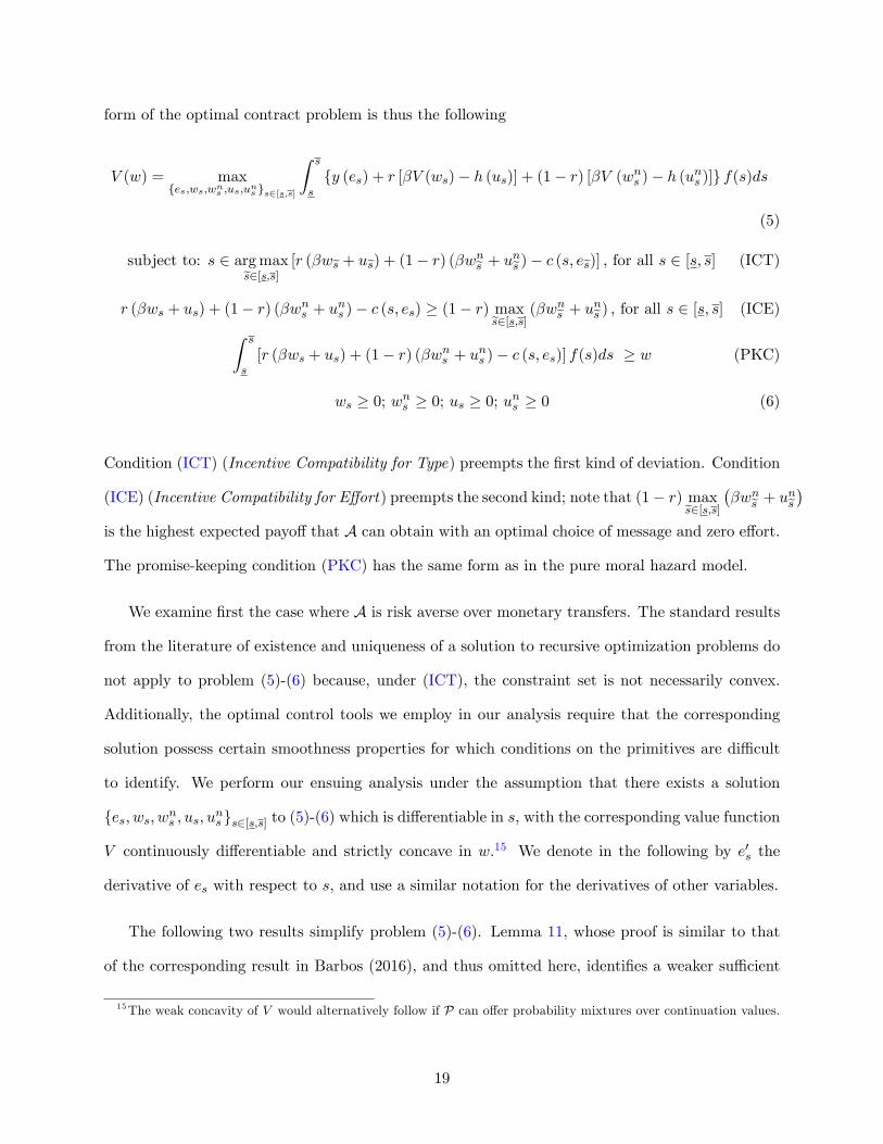
form of the optimal contract problem is thus the following

V (w) = maxfes;ws;wns ;us;uns gs2[s;s]

Z s

sfy (es) + r [�V (ws)� h (us)] + (1� r) [�V (wns )� h (uns )]g f(s)ds

(5)

subject to: s 2 argmaxes2[s;s] [r (�wes + ues) + (1� r) (�wnes + unes )� c (s; ees)] , for all s 2 [s; s] (ICT)

r (�ws + us) + (1� r) (�wns + uns )� c (s; es) � (1� r) maxes2[s;s] (�wnes + unes ) , for all s 2 [s; s] (ICE)Z s

s[r (�ws + us) + (1� r) (�wns + uns )� c (s; es)] f(s)ds � w (PKC)

ws � 0; wns � 0; us � 0; uns � 0 (6)

Condition (ICT) (Incentive Compatibility for Type) preempts the �rst kind of deviation. Condition

(ICE) (Incentive Compatibility for E¤ort) preempts the second kind; note that (1� r) maxes2[s;s]��wnes + unes �

is the highest expected payo¤ that A can obtain with an optimal choice of message and zero e¤ort.

The promise-keeping condition (PKC) has the same form as in the pure moral hazard model.

We examine �rst the case where A is risk averse over monetary transfers. The standard results

from the literature of existence and uniqueness of a solution to recursive optimization problems do

not apply to problem (5)-(6) because, under (ICT), the constraint set is not necessarily convex.

Additionally, the optimal control tools we employ in our analysis require that the corresponding

solution possess certain smoothness properties for which conditions on the primitives are di¢ cult

to identify. We perform our ensuing analysis under the assumption that there exists a solution

fes; ws; wns ; us; uns gs2[s;s] to (5)-(6) which is di¤erentiable in s, with the corresponding value function

V continuously di¤erentiable and strictly concave in w.15 We denote in the following by e0s the

derivative of es with respect to s, and use a similar notation for the derivatives of other variables.

The following two results simplify problem (5)-(6). Lemma 11, whose proof is similar to that

of the corresponding result in Barbos (2016), and thus omitted here, identi�es a weaker su¢ cient

15The weak concavity of V would alternatively follow if P can o¤er probability mixtures over continuation values.

19

condition (ICEW) (Weak Incentive Compatibility For E¤ort) for a contract to preempt shirking.

Speci�cally, it states that a contract which induces truthful type revelation, i.e., which satis�es

(ICT), will induce all agent types to exert e¤ort as long as it induces the least e¢ cient type s to

exert e¤ort. Lemma 12 validates in this setting the standard First Order Approach to contracting

problems with asymmetric information. Its proof is also similar to the proof of the result from

Barbos (2016), and therefore omitted. Accounting for the result of lemma 12, as in the standard

approach from the literature to such situations, in the following, we replace (ICT) with (ICTW)

(Weak Incentive Compatibility For Type) and assume that the constraint in (7) is satis�ed with

strict inequality. Barbos (2016) presents the analysis of the case where the constraint may bind.

Lemma 11 Any contract that satis�es (ICT) will satisfy (ICE) if and only if

r (�ws + us) + (1� r) (�wns + uns )� c (s; es) � (1� r) (�wns + uns ) , for all s 2 [s; s] (ICEW)

Lemma 12 A contract induces truthful type revelation for all s 2 [s; s] if and only if

e0s � 0 a.e. s 2 [s; s] (7)

r��w0s + u

0s

�+ (1� r)

��wn0s + u

n0s

�= ce(s; es)e

0s a.e. s 2 [s; s] (ICTW)

As in section 3, denote by w � inf fwjV 0(w) = �h0(0)g. Proposition 13 derives features of the

optimal contract which mirror properties of the contract under pure moral hazard, and have a

similar intuition. The proofs of all results from this section are presented in appendix A3.

Proposition 13 (i) For all s 2 [s; s], it is optimal to set ws � wns and us � uns ; (ii) For any

s 2 [s; s] for which (ICEW) does not bind, it is optimal to set ws = wns and us = uns ; (iii) us = 0

if and only if ws < w; (iv) uns = 0 if and only if wns < w; (v) ws > 0 for all s;

By parts (i) and (ii) of the proposition, a complying agent is always o¤ered at least as high

continuation values and wage-utilities when monitored as when not monitored; these variables are

20

equal for the types for which the incentive constraint that induces e¤ort does not bind. Parts (iii)

and (iv) show that the trade-o¤ between current and future payments is solved in the same manner

as in a situation without adverse selection: the current period transfers are zero when the cost of

delivering them through promises about future transfers is low. Part (v) is a consequence of the

fact that ws is the primary tool for incentivizing e¤ort and therefore must be strictly positive since

the contract implements strictly positive e¤ort for all types.

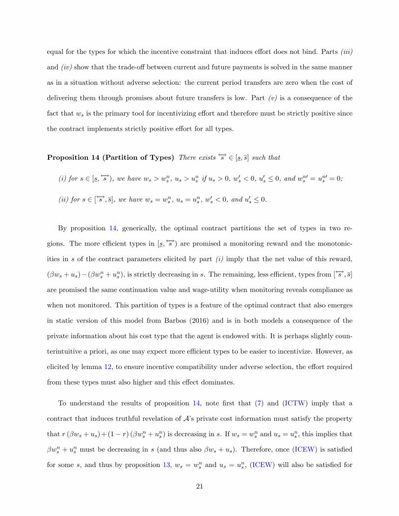
Proposition 14 (Partition of Types) There exists !s 2 [s; s] such that

(i) for s 2 [s; !s ), we have ws > wns , us > uns if us > 0, w0s < 0, u0s � 0, and wn0s = un0s = 0;

(ii) for s 2 [ !s ; s], we have ws = wns , us = uns , w0s < 0, and u0s � 0.

By proposition 14, generically, the optimal contract partitions the set of types in two re-

gions. The more e¢ cient types in [s; !s ) are promised a monitoring reward and the monotonic-

ities in s of the contract parameters elicited by part (i) imply that the net value of this reward,

(�ws + us)� (�wns + uns ), is strictly decreasing in s. The remaining, less e¢ cient, types from [ !s ; s]

are promised the same continuation value and wage-utility when monitoring reveals compliance as

when not monitored. This partition of types is a feature of the optimal contract that also emerges

in static version of this model from Barbos (2016) and is in both models a consequence of the

private information about his cost type that the agent is endowed with. It is perhaps slightly coun-

terintuitive a priori, as one may expect more e¢ cient types to be easier to incentivize. However, as

elicited by lemma 12, to ensure incentive compatibility under adverse selection, the e¤ort required

from these types must also higher and this e¤ect dominates.

To understand the results of proposition 14, note �rst that (7) and (ICTW) imply that a

contract that induces truthful revelation of A�s private cost information must satisfy the property

that r (�ws + us)+(1� r) (�wns + uns ) is decreasing in s. If ws = wns and us = uns , this implies that

�wns + uns must be decreasing in s (and thus also �ws + us). Therefore, once (ICEW) is satis�ed

for some s, and thus by proposition 13, ws = wns and us = uns , (ICEW) will also be satis�ed for

21

all higher values of s. The monotonicities of wns and uns on [s;

!s ) follow from the fact that it is

feasible to provide incentives for truthful type revelation by employing only ws and us, and thus to

minimize the variance in the set of future continuation values and A�s risk exposure, respectively,

wns and uns are optimally constant on [s;

!s ). From these, it follows that �ws + us is decreasing in

s on the whole interval [s; s]. The fact that both ws and us are in fact decreasing in s is then a

consequence of the fact that, optimally, the marginal costs of delivering utility to A through current

and future transfers, respectively, must be equal whenever us > 0.

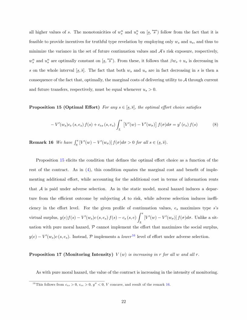
Proposition 15 (Optimal E¤ort) For any s 2 [s; s], the optimal e¤ort choice satis�es

� V 0(ws)ce (s; es) f(s) + ces (s; es)Z s

s

�V 0(w)� V 0(w�)

�f(�)d� = y0 (es) f(s) (8)

Remark 16 We haveR ss [V

0(w)� V 0(w�)] f(�)d� > 0 for all s 2 (s; s).

Proposition 15 elicits the condition that de�nes the optimal e¤ort choice as a function of the

rest of the contract. As in (4), this condition equates the marginal cost and bene�t of imple-

menting additional e¤ort, while accounting for the additional cost in terms of information rents

that A is paid under adverse selection. As in the static model, moral hazard induces a depar-

ture from the e¢ cient outcome by subjecting A to risk, while adverse selection induces ine¢ -

ciency in the e¤ort level. For the given pro�le of continuation values, es maximizes type s�s

virtual surplus, y(e)f(s)� V 0(ws)c (s; es) f(s)� cs (s; e)Z s

s[V 0(w)� V 0(w�)] f(�)d�. Unlike a sit-

uation with pure moral hazard, P cannot implement the e¤ort that maximizes the social surplus,

y(e)� V 0(ws)c (s; es). Instead, P implements a lower16 level of e¤ort under adverse selection.

Proposition 17 (Monitoring Intensity) V (w) is increasing in r for all w and all r.

As with pure moral hazard, the value of the contract is increasing in the intensity of monitoring.

16This follows from ces > 0, cee > 0, y00 < 0, V concave, and result of the remark 16.

22

The last result of the section identi�es a condition under which the �rst best outcome can

be implemented under moral hazard and adverse selection when the agent is risk neutral. This

condition ensures that the limited liability constraint of the agent is not violated by a contract that

induces truthful type revelation and implements the �rst best e¤ort level. As in the rest of the

analysis in this section, we assume that e0s > 0 for all s 2 [s; s], i.e., that it is optimal to implement

strictly positive e¤ort in all states under full information.

Proposition 18 (Risk Neutral Agent) If A is risk neutral and c�s; e0s

��R ss cs

�s; e0s

�F (s)ds �

0, the value of the optimal contract under moral hazard and adverse selection equals the value of

the optimal contract under full information.

5 Conclusion

In this paper we characterize optimal contracts with random monitoring in a repeated contractual

relationship where incentives can be provided both with current transfers and promises about future

transfers. The shape of the optimal contract is determined by the solution to two trade-o¤s that

emerge in this context and their interplay. The �rst trade-o¤ is between incentive provision and

e¢ ciency. Speci�cally, since incentives to exert e¤ort under randommonitoring can only be provided

with the contract variables speci�ed for contingencies where monitoring is executed, these variables

must be su¢ ciently high, whereas e¢ ciency requires minimizing the variance in the agent�s current

and future income. The second trade-o¤ is that between delivering utility to the agent through

current and future transfers. The solution to the �rst trade-o¤ involves promising the agent a

reward when monitoring reveals compliance relative to the terms of the contract promised when

no monitoring is performed. This reward comes in the form of higher current period transfers of

promises about future compensation. As time passes, the size of the reward decreases as the agent

becomes rich enough that the threat of a loss of the promised stream of future income provides the

agent with su¢ cient incentives for complying with the e¤ort recommendation.

23

Appendix

Appendix A1. Proofs for Section 3.

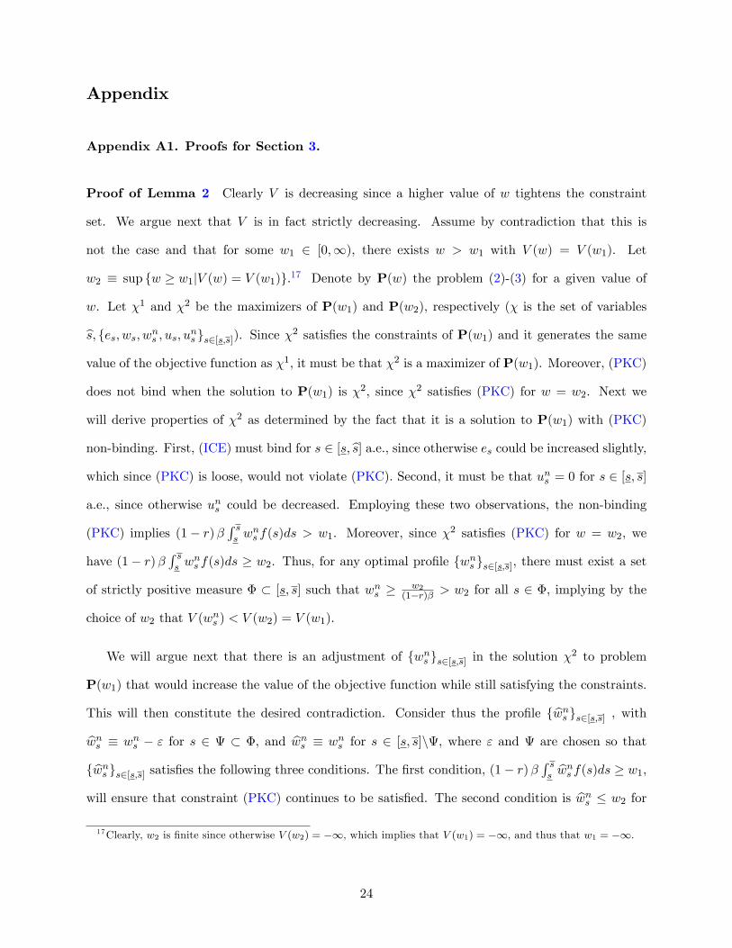
Proof of Lemma 2 Clearly V is decreasing since a higher value of w tightens the constraint

set. We argue next that V is in fact strictly decreasing. Assume by contradiction that this is

not the case and that for some w1 2 [0;1), there exists w > w1 with V (w) = V (w1). Let

w2 � sup fw � w1jV (w) = V (w1)g.17 Denote by P(w) the problem (2)-(3) for a given value of

w. Let �1 and �2 be the maximizers of P(w1) and P(w2), respectively (� is the set of variables

bs; fes; ws; wns ; us; uns gs2[s;s]). Since �2 satis�es the constraints of P(w1) and it generates the samevalue of the objective function as �1, it must be that �2 is a maximizer of P(w1). Moreover, (PKC)

does not bind when the solution to P(w1) is �2, since �2 satis�es (PKC) for w = w2. Next we

will derive properties of �2 as determined by the fact that it is a solution to P(w1) with (PKC)

non-binding. First, (ICE) must bind for s 2 [s; bs] a.e., since otherwise es could be increased slightly,which since (PKC) is loose, would not violate (PKC). Second, it must be that uns = 0 for s 2 [s; s]

a.e., since otherwise uns could be decreased. Employing these two observations, the non-binding

(PKC) implies (1� r)�R ss w

ns f(s)ds > w1. Moreover, since �2 satis�es (PKC) for w = w2, we

have (1� r)�R ss w

ns f(s)ds � w2. Thus, for any optimal pro�le fwns gs2[s;s], there must exist a set

of strictly positive measure � � [s; s] such that wns � w2(1�r)� > w2 for all s 2 �, implying by the

choice of w2 that V (wns ) < V (w2) = V (w1).

We will argue next that there is an adjustment of fwns gs2[s;s] in the solution �2 to problem

P(w1) that would increase the value of the objective function while still satisfying the constraints.

This will then constitute the desired contradiction. Consider thus the pro�le f bwns gs2[s;s] , withbwns � wns � " for s 2 � �, and bwns � wns for s 2 [s; s]n, where " and are chosen so that

f bwns gs2[s;s] satis�es the following three conditions. The �rst condition, (1� r)� R ss bwns f(s)ds � w1,will ensure that constraint (PKC) continues to be satis�ed. The second condition is bwns � w2 for17Clearly, w2 is �nite since otherwise V (w2) = �1, which implies that V (w1) = �1, and thus that w1 = �1.

24

all s 2 ; since this implies that V ( bwns ) � V (w2) > V (wns ), it will follow that this adjustment

strictly increases the value of the objective function in problem P(w1). The third condition is that

bwns � 0, i.e., that " � wns . Now, since (1� r)� R ss wns f(s)ds � w2, we have (1� r)� R ss bwns f(s)ds �w2� (1� r)�"

R f(s)ds, and thus for the �rst condition to be satis�ed, we need " �

w2�w1(1�r)�

R f(s)ds

(*). The second condition can be rewritten as wns � w2 � ". Since wns � w2(1�r)� > w2 for all s 2 �

implies wns �w2 � w2(1�r)� �w2, for the second condition to be satis�ed is would be enough to ensure

that " � w2(1�r)� �w2 (**). Finally, to satisfy the third condition, since w

ns � w2

(1�r)� for all s 2 �, it

is enough that " � w2(1�r)� (***). Thus, a value " exists satisfying conditions (*), (**), and (***) if

minn

w2�w1(1�r)�

R f(s)ds

; w2(1�r)�

o> w2

(1�r)� �w2, i.e., w2�w1 > w2 [1� (1� r)�]R f(s)ds. This can be

ensured by choosing the set of su¢ ciently small, but strictly positive measure. This completes

the proof of the fact that V is strictly decreasing.

Note that this immediately implies that (PKC) must bind for all w in a solution to problem

(2)-(3) since otherwise V would be constant on intervals where (PKC) does not bind. �

We continue by introducing several preliminary concepts and results that will be employed in

the ensuing analysis for comparative statics of the contract variables.

De�nition 19 A correspondence H : R ! 2R is increasing (strictly increasing) if for any x > y,

and x0 2 H(x), y0 2 H(y), we have x0 � y0 (x0 > y0).

Lemma 20 Let V be a convex function with subdi¤erential @V and g (x) be a increasing function.

Then the correspondence @V (g (x)) is increasing in x.

Proof. This follows from the fact that @V (g (x)) =n� 2 R

���V 0�(g (x)) � � � V 0+(g (x))o and

Theorem 24.1 in Rockafellar (1970) which states that if z1 < � < z2 and V is convex then V0+(z1) �

V0�(�) � V

0+(�) � V

0+(z2). In particular, note that if x2 > x1, and thus g (x2) > g (x1), then the

theorem implies V0+(g (x1)) < V

0�(g (x2)), which given the de�nition of the subdi¤erential implies

that for any �1 2 @V (g (x1))and �2 2 @V (g (x2)), it must be that �1 � �2. �

25

Lemma 21 Let H(s; e) be a correspondence which is increasing in s and strictly increasing in e.

For any s, de�ne the correspondence es � fe j0 2 H(s; e)g. Then es is a decreasing function of s.

If in addition, H(s; e) is strictly increasing in s, then es is a strictly decreasing function.

Proof. Consider two values s2 > s1 and let �1 2 es1 and �2 2 es2 . If �2 > �1, then for any

x2 2 H(s2; �2) and x1 2 H(s1; �1), we would have x2 > x1 given the monotonicity of H in the

two variables. But then 0 2 H(s2; �2) \H(s1; �1), as required by the de�nition of es, could not be

satis�ed. We conclude then that it must be that �2 � �1. Moreover, if H(s; e) is strictly increasing

in s then �2 < �1. These imply that es is a decreasing correspondence in s, and strictly decreasing

if H(s; e) is strictly increasing in s. By a similar argument, since H is strictly increasing in e, it

follows that for any s, the set fe j0 2 H(s; e)g must be a singleton, and thus es is a function. �

To solve problem (2)-(3), we �rst rewrite (ICE) as 1s<bs [r (�ws + us)� c (s; es)] � 0, for all

s 2 [s; s], and let �sf(s) be the nonnegative Lagrange multipliers associated with it. Also, we let

� 0 be the multiplier on (PKC). The Lagrangian associated with problem (2)-(3) is then

L �Z s

sfy (es) + r [�V (ws)� h (us)] + (1� r) [�V (wns )� h (uns )]g f(s)ds

+

Z s

s1s<bs�s [r (�ws + us)� c (s; es)] f(s)ds+

+

�Z s

s[r (�ws + us) + (1� r) (�wns + uns )� c (s; es)] f(s)ds � w

�

The corresponding necessary �rst-order conditions (cancelling out f(s), r, 1� r, or �) are

@L@us

= �h0(us) + 1s<bs�s + � 0, and = 0 if us > 0 (9)

@L@uns

= �h0(uns ) + � 0, and = 0 if uns > 0 (10)

@L@ws

= 0) 1s<bs�s + 2 �@V (ws), if ws > 0 (11)

@L@wns

= 0) 2 �@V (wns ), if wns > 0 (12)

@L@es

= y0(es)� 1s<bs�sce (s; es)� ce (s; es) � 0, and = 0 if s 2 [s; bs) (13)

26

where for (13) we used the fact that es > 0 if and only if s 2 [s; bs). As one cannot genericallyguarantee the di¤erentiability of V ,18 the conditions (11) and (12) are written in terms of its

superdi¤erential. In addition, the necessary �rst order conditions with respect to ws and wns , for

the cases where ws = 0 and wns = 0, respectively, are@L@ws� 0) 1s<bs�s+ +V 0(ws) � 0, if ws = 0,

and @L@wns� 0 ) + V 0(wns ) � 0, if wns = 0. Finally, by the Envelope Theorem with respect to w,

we have that @L@w = � 2 @V (w).

Proof of Proposition 3 Since from the Envelope Theorem we have 2 �@V (w), (12) implies

that, for all s 2 [s; s], if wns > 0, then it must be that @V (w) \ @V (wns ) 6= ?. Since V is concave,

it is therefore optimal to set wns = w (if V is strictly concave in a neighbourhood around w, then

setting wns = w is the unique optimal choice; if V is linear around w, then this is one of the optimal

choices for wns ). On the other hand, if wns = 0 then the necessary �rst order condition with respect

to ws is +V 0(wns ) � 0, which since wns = 0 implies that V 0(0) � � 2 @V (w). Since V is concave

and the superdi¤erential of a concave function is a decreasing correspondence (this is an immediate

implication of Theorem 24.1 in Rockafellar (1970), stated in the proof of lemma 20 above), it follows

that w � 0, i.e., that w = 0. We conclude that in both situations, it must be that wns = w , for

all s 2 [s; s]. This demonstrates part (i) of the proposition. Similarly, for all s 2 [bs; s], from (11)

and the corresponding �rst order condition for the case where ws = 0, imply that ws = w for all

s 2 [bs; s], demonstrating the statements from part (ii) of the proposition for these types. Now, for

the remaining statements from parts (ii) and (iii) that pertain to s 2 [s; bs), note that 2 �@V (w)and (11) imply for all s 2 [s; bs) with ws > 0 that

�s 2 �@V (ws) + @V (w) (14)

which since �s � 0 and V is concave implies ws � w. In addition, when (ICE) does not bind and

thus �s = 0, it is optimal to set ws = w. Finally, note that if ws = 0 for some s 2 [s; bs), then the18The standard results that deliver di¤erentiability require that the solution be interior to the constrained set.

Since this is not necessarily the case here, we cannot apply results such as Theorem 4.11 in Stokey and Lucas (1989)to conclude that V is di¤erentiable.

27

necessary �rst order condition is �s+ +V0(ws) � 0. This implies that �s+V 0(0) � � 2 @V (w),

and thus since �s � 0 and � 0 that w = 0 (since V 0(0) � � 2 @V (w) and V concave) and then

that = �s = 0. This completes the proof of the proposition 3. �

Proof of Proposition 4 First, from (10) it follows that uns is constant in s and thus part (i) of

the proposition. To see this, note that the only case where this is not immediate is if uns > 0 for

s 2 S, and uns = 0 for the remaining s 2 [s; s]nS, where S is a proper subset of [s; s]. Now, if this

was the case, then (10) would imply that uns = uz > 0 for s 2 S, = h0(uz) and � h0(0). From

the latter two implications, we would have h0(uz) � h0(0), and thus uz = 0 since h is convex; this

delivers the contradiction. Parts (ii) and (iii) follow from (9) and (10), the fact that h is convex,

and that �s � 0 with �s = 0 when (ICE) does not bind.

Now, for part (iv), note that when w < w, for any � 2 @V (w) ��� 2 R

��V 0+(w) � � � V 0�(w)and any u � 0, we have that � �V 0+(w) � �V 0+(w) = h0(0), where the second inequality follows

from the fact that �V is convex and from Theorem 24.1 in Rockafellar (1970), while the equality

from the de�nition of w. Therefore, �h0(u)+ � �h0(u)+h0(0), which since h is strictly increasing,

implies �h0(u)+ < 0 for any u > 0. It follows then from (9) and (10) that it must be that us = 0

for any s 2 [bs; s], and that uns = 0 for any s 2 [s; s], respectively.Finally, for part (v) of the proposition, if ws < w for some s 2 [s; bs), we have for any u > 0 that

�h0(u)+�s+ < 0 since by (11) �s+ 2 �@V (ws), and thus �s+ < �V 0+(w) = h0(0). Therefore,

if ws < w, then us = 0 as stated by part (v). Note also here that if w � w and �s = 0, then us = 0,

whereas if �s > 0, then it is possible that us > 0 since the condition �h0(0)+�s+ = 0 is attained

at smaller values of w than w. We cannot, thus, substitute w for ws in the text of part (v). �

Proof of Proposition 5 Part (i) of the proposition follows immediately from (11) and (13).

We will prove next part (ii). Consider �rst any value w 2 [0; w) and any s 2 [s; bs) with us = 0.When (ICE) does not bind for some type s, then as shown in proposition 3(iii), we have ws = w.

28

Substituting this into (4), it follows that es must satisfy

0 2 �y0(es) + ce (s; es) [�@V (w)] (15)

Since @V (w) is independent of s and e, it follows that the correspondence H(s; e) � �y0(e) +

ce (s; e) [�@V (w)] is strictly increasing in e and s (for the latter, we use the fact that @V (w) �

(�1; 0)). Therefore, by lemma 21 es is strictly decreasing in s. When (ICE) binds, by our assump-

tion that us = 0, we have ws = 1r� c (s; es), and thus from (11) it follows �s+ 2 �@V

�1r� c (s; es)

�.

Substituting �s + from (13) (which is satis�ed with equality since es > 0 when s 2 [s; bs)) intothis, we obtain that es satis�es

y0(es)ce(s;es)

2 �@V�1r� c (s; es)

�which can be rewritten as

0 2 �y0(es) + ce (s; es)��@V

�1

r�c (s; es)

��(16)

Now, ce > 0 and the fact that V � �V is strictly increasing and convex imply that the cor-

respondence @V�1r� c (s; e)

�is increasing in e and s by lemma 20. Let H(s; e) � �y0(e) +

ce (s; e)h�@V

�1r� c (s; e)

�i=n�y0(e) + ce (s; e)x

���x 2 �@V � 1r� c (s; e)

�o, and note that y00 < 0,

cee > 0, cs > 0, ces > 0 and @V�1r� c (s; e)

�� (�1; 0) imply that H(s; e) is strictly increasing in e

and s. Therefore, again by lemma 21, es is strictly decreasing in s.

Consider now any value w � w or any value w 2 [0; w) and s 2 [s; bs) such that us > 0, i.e.,

values of w for which transfers towards the agent under various contingencies are not all zero. If

(ICE) does not bind for some type s, then the analysis of the comparative statics of es with respect

to s is identical to that of the corresponding case for situations where us = 0 since these induced

utilities do not enter the equation (15) that de�nes the optimal value of es. If (ICE) binds, then

ws =1�r c (s; es)�

us� . From (9), since us > 0 we have �s + = h

0(us), which substituted into (13)

implies y0(es) � h0(us)ce (s; es) = 0, and therefore that us = (h0)�1�y0(es)ce(s;es)

�. On the other hand,

since (9) and (11) imply that h0(us) 2 �@V (ws), it follows by substituting terms derived above

into y0(es)�h0(us)ce (s; es) = 0 that y0(es)ce(s;es)

2 �@V�1�r c (s; es)�

1� (h

0)�1�y0(es)ce(s;es)

��, which can be

29

rewritten as

0 2 �y0(es) + ce (s; es)��@V

�1

�rc (s; es)�

1

�

�h0��1� y0(es)

ce (s; es)

���(17)

Note now that

@

@e

�1

�rc (s; e)� 1

�

�h0��1� y0(e)

ce (s; e)

��=

=1

�rce (s; e)�

1

�

�h00��h0��1� y0(e)

ce (s; e)

����1 y00(e)ce (s; e)� y0(e)cee (s; e)[ce (s; e)]

2

Since h is strictly convex, the properties of the functions y (�) and c (�; �) imply that this partial

derivative is strictly positive. Similarly, the partial derivative of the same expression with re-

spect to s is strictly positive. Therefore, applying lemma 20, it follows that the subdi¤erential

@V�1�r c (s; e)�

1� (h

0)�1�y0(e)ce(s;e)

��is increasing in e and s, and thus that the correspondence in

(17) is strictly increasing in e and s (the latter because the subdi¤erential is strictly positive). It

follows then by lemma 21 that es is strictly decreasing in s.

We mention here that if (ICE) binds, even under an additional assumption of di¤erentiability

of V , the signs of dwsds and dusds are generically undetermined. One can use the Implicit Function

Theorem to derive the expression for dwsds from the system in (es; ws) made of equations y0(es) �

V 0(ws)ce (s; es) = 0 and h0�1r c(s; es)� �ws

�+ V 0(ws) = 0, which can be obtained from the set of

necessary �rst order conditions, but the sign of dwsds is undetermined. Similarly, one can derive a

system of equations in (es; us) and conclude that the sign of dusds is undetermined. �

Proof of Lemma 6 Note that for any w and any s 2 [s; bs), (ICE) binds if and only if �w+us <c (s; es), where es is the solution to (16) or (17) for that particular value of s. Since (16) and (17)

are independent of w, it follows that when (ICE) binds, es is constant in w. Moreover, as argued

in the proof of proposition 5, us equals either 0 or (h0)�1�y0(es)ce(s;es)

�, which since es is independent

of w, implies that us is also independent of w. We conclude that the condition �w + us < c (s; es)

30

holds for all small enough w. Therefore, there exists ews � inf fw j�w + us � c (s; es)g, such that(ICE) binds for all w � ews.

On the other hand, as w increases immediately above ews, and thus (ICE) does not bind, es isdetermined by (15). Since the correspondence H(w; e) � �y0(e) + ce (s; e) [�@V (w)] is increasing

in w (because of the concavity of V ), and strictly increasing in e (as we showed in the proof of

proposition 5), we conclude that es is decreasing in w. As for us, if us > 0 and (ICE) does not

bind (and thus �s = 0), then from (9) and 2 �@V (w), it follows that 0 2 �h0(us) � @V (w).

Since H(u;w) � �h0(u) � @V (w) is strictly decreasing in u and increasing w, it follows that us is

increasing in w. Finally, when (ICE) does not bind, ws = w is strictly increasing in w. We conclude

that once (ICE) does not bind for some value w, it will continue to be nonbinding for all higher

values of w since, as w increases, �w+us strictly increases, while c (s; es) decreases because es does

so. This completes the proof of the lemma 6. �

Proof of Proposition 7 We already argued in the proof of lemma 6 that whenever (ICE) binds,

es and us are constant in w. Since (ICE) binding implies ws = 1�r c (s; es)�

us� , ws must be constant

as well. Therefore, ws is constant in w for w 2 [0; ews]. When (ICE) does not bind, as also shownin the proof of claim 6, es is decreasing in w, and us is increasing in w, whereas, optimally, we

have ws = w, and thus ws is strictly increasing in w. Moreover, since ws is continuous in w, the

fact that ws = w when w = ews implies that on [0; ews], it must be that ws = ews. We examine nowhow wns and u

ns depend on w. First, w

ns is strictly increasing since, optimally, w

ns = w. Second,

when uns > 0, we have from (10), (12), and the fact that wns = w, that 0 2 �h0(uns )�@V (w), which

implies then that uns is increasing in w.

Next, we investigate how the threshold bs varies with w. Note that in the above we only showedthat es is decreasing in w for s 2 [s; bs), but in principle bs could still increase when w increases; wewill argue now that this is not the case. We consider the case where the density f(s) is continuous

so that the Lagrangian L is continuously di¤erentiable and the �rst order necessary condition has

the standard form. The analysis of the general case is more tedious, but follows the same approach.

31

Employing thus the �ndings of propositions 3 and 4, L can be rewritten as

L =

Z bssfy (es) + r [�V (ws)� h (us)] + (1� r) [�V (w)� h (uz)]g f(s)ds

+

Z s

bs [�V (w)� h (uz)] f(s)ds+Z bss�s [r (�ws + us)� c (s; es)] f(s)ds+

+

(Z bss[r (�ws + us) + (1� r) (�w + uz)� c (s; es)] f(s)ds +

Z s

bs (�w + uz) f(s)ds� w)

Since L is continuously di¤erentiable as the integral of a continuous function, the necessary condition

for the optimality of bs, when bs 2 (s; s) is @L@bs = 0. Employing the complementary slackness conditionon constraint (ICE), @L@bs = 0 becomes

y (ebs) + r [�V (wbs)� h (ubs)]� r [�V (w)� h (uz)] + f[r (�wbs + ubs)� r (�w + uz)� c (bs; ebs)]g = 0(18)

Consider now for any w, any s 2 [s; bs) with us = 0. By proposition 5, uz = 0 as well. (18)

becomes then

y (ebs) + r� [V (wbs)� V (w)] + [r� (wbs � w)� c (bs; ebs)] = 0 (19)

If (ICE) does not bind, then wbs = w and thus (19) becomes y (ebs) � c (bs; ebs) = 0. Since 2

�@V (w), this can be rewritten as 0 2 H(w; bs) � �y (ebs) + c (bs; ebs) [�@V (w)]. Since ebs andwbs are chosen optimally, by the Envelope Theorem, we have @

@bs f�y (ebs) + c (bs; ebs) [�@V (w)]g =�cs (bs; ebs) @V (wbs) � (0;1). On the other hand, since V is concave, the correspondence �@V (w)

is increasing in w, and therefore so is �y (ebs)+ c (bs; ebs) [�@V (w)]. We conclude the correspondenceH(w; bs) is strictly increasing in bs and increasing in w. This implies by lemma 21 that bs is decreasingin w as claimed by the proposition. If (ICE) binds, then wbs = c(bs;ebs)

�r and (19) becomes y (ebs) +r�hV�c(bs;ebs)�r

�� V (w)

i+

nhr��c(bs;ebs)�r � w

�� c (bs; ebs)io = 0, which since 2 �@V (w) can be

rewritten as 0 2 H(w; bs) � �y (ebs) + r� h�V � c(bs;ebs)�r

�+ V (w)� w@V (w)

i. Then cs > 0 and

the fact that V strictly decreasing on (0;1), where c(bs;ebs)�r lies, imply that �V

�c(bs;ebs)�r

�is strictly

increasing in bs and thus immediately that H(w; bs) is strictly increasing as well. On the other hand,32

let x 2 @V (w) and x0 2 @V (w0), for some w0 > w; since V is concave it must be that x0 � x.

Note then that we have V (w) � V (w0) � x0 (w � w0) � xw � x0w0 , where the �rst inequality

follows from the de�nition of the superdi¤erential at w0 of the concave function V and x0 2 @V (w0)

(see, for instance, Rockafellar (1970), pp. 214-215), while the second from x0 � x. Therefore,

V (w0)�w0x0 � V (w)�wx, which implies that the correspondence V (w)�w@V (w) is increasing

in w. It follows that H(w; bs) is increasing in w, and thus by lemma 21 that bs is decreasing in w.Finally, consider any value w for which ubs > 0. If (ICE) does not bind, by proposition 3, we

have us = uz, and therefore (18) becomes y (ebs) � c (bs; ebs) = 0, where we also used the fact thatwbs = w. As argued above, this implies that bs is decreasing in w. If (ICE) binds, then wbs = c(bs;ebs)

�r ,

and therefore employing also the facts that 2 �@V (w) and that h0(uz) = whenever uz > 0,

(18) becomes

0 2 H(w; bs) � �y (ebs) + r� ��V �c (bs; ebs)�r

�+ V (w)� w@V (w)

�+ rh (ubs) + rA(w; bs),

where A(w; bs) � ft : t = �h (uz) + uzx, with h0 (uz) = x 2 �@V (w)g (20)

Since we have already showed above that �y (ebs)+r� h�V � c(bs;ebs)�r

�+ V (w)� w@V (w)

iis strictly

increasing in bs and increasing w, we aim to show that the correspondence h0(ubs) +A(w; bs) has thesame properties. Note that from (9) and (11) we have h0(ubs) 2 �@V � c(bs;ebs)�r

�, while from (10) and

(12), we have h0(uz) 2 �@V (w) for any bs. Therefore, h (ubs) is independent of w, while A(w; bs)is independent of bs. Since V is concave and cs > 0, h0(ubs) 2 �@V � c(bs;ebs)�r

�implies immediately

that ubs, and therefore h (ubs), are increasing in bs. To complete the argument it is then enoughto show that A(w; bs) is increasing in w. Consider some arbitrary values w0 > w, then arbitrary

values x0 2 �@V (w0) and x 2 �@V (w), and let z0 � (h0)�1(x0) and z � (h0)�1(x). We will

show that �h (z0) + z0x0 � �h (z) + zx which will imply that A(w; bs) is indeed increasing inw. Since h is strictly convex, h (z0) � h(z) < h0(z0)(z0 � z), and so it is enough to show that

z0x0 � zx � h0(z0)(z0 � z), i.e., that z0 [x0 � h0(z0)] � z[x � h0(z0)]. Since V is concave, x0 � x,

and thus h0 (z0) � h0(z), which immediately imply that x � h0(z0). Together with x0 = h0(z0), this

33

implies that z0 [x0 � h0(z0)] = 0 � z[x � h0(z0)]. We conclude that H(w; bs), as de�ned in (20), isstrictly increasing in bs and increasing in w, and thus that bs is again decreasing in w. It is immediatethen to argue that the same property holds for the treshold bs that maximizes L instead of bL . �Proof of Proposition 8 For the �rst part of the proposition note that for any continuation

value w at the beginning of a given period, P can satisfy A�s incentive constraints in all future

periods with the following set of choice variables: es = 0, ws = w, and us = (1� �)w for all

s 2 [s; s]. These correspond to A being retired and delivered utility (1� �)w in every period

for perpetuity. The discounted present value of the contract to P corresponding to this set of

choice variables is � 11��h((1� �)w). Therefore, if V solves problem (2)-(3), then it must be that

V (w) � � 11��h((1� �)w) for all w.

For the second part of the statement in (i), note that if, optimally, es = 0 for all s 2 [s; s],

then P�s problem is that of maximizing the objective function in (2) subject to the participation

constraint in (PKC) and the non-negativity of the choice variables. By propositions 3 and 4, in

the corresponding solution, we have ws = w for all s and us = uz for all s and some uz � 0.

Therefore, the binding (PKC) becomes �w + uz = w, i.e., uz = (1� �)w. Therefore, V (w) =

�h((1� �)w) + �V (w), implying indeed that V (w) = � 11��h((1� �)w).

For part (ii), we only need to examine the case where w is �nite. First, since V (w) �

� 11��h((1� �)w), V (w) = �

11��h((1� �)w), and �

11��h((1� �)w) is concave and di¤eren-

tiable in w, employing Theorem 4.10 from Stokey and Lucas (1989), it follows that V is dif-

ferentiable at w and that V 0(w) = �h0((1� �)w). Next, we will show that es = 0 for all

s 2 [s; s] at w. To this aim, assume by contradiction that at w, it is optimal instead to have

es > 0 for all s 2 [s; bs), for some bs 2 [s; s] with F (bs) > 0. Let then (S1; S2) be the parti-

tion of [s; bs] such that (ICE) binds for all s 2 S1 and does not bind for all s 2 S2, and de-

note m(Si) �Rs2Si f(s)ds. By propositions 3 and 4, we have then ws = w and us = uz for

all s 2 [bs; s] [ S2, and wns = w and uns = uz for all s 2 [s; s]. In addition, r (�ws + us) �

c (s; es) = 0 for all s 2 S1. Employing these, it follows that the binding condition in (PKC) be-

34

comes��w + uz

�[(1� r)m(S1) +m(S2) + 1� F (bs)] � Rs2S2 c(s; es)f(s)ds = w. Therefore, uz =

1(1�r)m(S1)+m(S2)+1�F (bs)

hf1� � [(1� r)m(S1) +m(S2) + 1� F (bs)]gw + Rs2S2 c(s; es)f(s)dsi > 0.

Since F (bs) > 0, we have then that uz > (1� �)w, which since h is strictly convex implies

h0(uz) > h0((1� �)w). However, conditions (10) and (12) imply that at optimum, we must have

h0(uz) 2 �@V (w). As argued above, @V (w) = f�h0((1� �)w)g, and thus h0(uz) = h0((1� �)w).

This provides the desired contradiction. Finally, since by proposition 7, es is decreasing in w, it

must be that es = 0 for all s 2 [s; s] and w � w. �

Proof of Proposition 9 Using the multipliers from the de�nition of L, the per-period change in

P�s payo¤ from a small increase in r is �V =R bss f[�V (ws)� h (us)]� [�V (w

ns )� h (uns )]g f(s)ds+R bs

s �s (�ws + us) f(s)ds + R bss [(�ws + us)� (�w

ns + u

ns )] f(s)ds, which can be written as �V =R bs

s �Vsf(s)ds, where

�Vs � � [V (ws) + ( + �s)ws � V (wns )� wns ] + [h (uns )� uns � h (us) + ( + �s)us] (21)

We will argue that both terms from (21) are nonnegative. First, note that since +�s 2 �@V (ws)

and 2 �V (wns ), while by proposition 3 we have ws � wns , to show that the �rst term is non-

negative, it would be enough for the correspondence V (w) � w@V (w) to be increasing, which has

already been shown in the proof of proposition 7. As for the second term in (21), note �rst that

if us = 0, then by proposition 3, uns = 0 as well and thus the term is 0. If us > 0, then from (9)

it follows that + �s = h0 (us), while from (10), we have � h0(uns ). It is enough then to show

that [h (uns )� h0 (uns )uns ] � [h (us)� h0 (us)us] � 0. Since by proposition 3, we have us � uns , it is

enough to show that the function h (u)�h0 (u)u is decreasing, which follows immediately by taking

its derivative and accounting for the fact that h is convex. We conclude that, indeed, �Vs � 0, and

thus �V � 0. Since the per-period change to P�s payo¤ from a small increase in r is positive, it

follows that V (w), which is the discounted sum of future period payo¤s, is increasing in r.19 �

19This argument is similar to the one employed in the proof of lemma 1 in Kovrijnykh (2013).

35

Proof of Proposition 1 The recursive representation of the optimal contract problem is

V (w) = maxfes;ws;usgs2[s;s]

Z s

sfy (es) + r [�V (ws)� h (us)]g f(s)ds (22)

s.t.Z s

s[r (�ws + us)� c (s; es)] f(s)ds � w (23)

The Lagrangian is L �fy (es) + r [�V (ws)� h (us)]g f(s) + f[r (�ws + us)� c (s; es)] f(s)� wg,

with 2 R+, and so the necessary �rst order conditions, after cancelling out terms, are

@L@us

= �h0(us) + � 0, and = 0 if us > 0 (24)

@L@es

= 0) y0(es)� ce (s; es) � 0, and = 0 if es > 0 (25)

@L@ws

= 0) 0 2 @V (ws) + if ws > 0;@L@ws

� 0) V 0(ws) + � 0 if ws = 0 (26)

From (24), it follows that there exists u0 2 R+ such that for all s 2 [s; s], with us > 0, we have

us = u0. Assume now by contradiction that u0 > 0 and that us = 0 for some s 2 [s; s]. From

(24) it follows then that �h0(0) + � 0, which since also from (24), we have = h0(u0), implies

that �h0(0) + h0(u0) � 0. This contradicts the fact that h is strictly convex. Therefore, it must be

that us = u0 for all s 2 [s; s], with u0 potentially being equal to 0. Similarly, from (26), using the

fact that V is concave (because P can o¤er lotteries over continuation values), it follows that there

exists w0 � 0 such that it is optimal that for all s 2 [s; s] to set ws = w0.20 Using the Envelope

Theorem on problem (22)-(23), we have 2 @L@w = �@V (w), which combined with (26), implies

that it is optimal to set w0 = w. Therefore, in the �rst period of the contract, when the value

promised to the agent is 0, it is optimal to set w0 = 0, implying that at the beginning of the second

stage, the agent is again promised a value equal to 0. By induction, he is promised a value 0 at the

beginning of every period. Since he must consume, it follows that u0 > 0. Finally, condition (1)

from the text of the proposition follows immediately from (24) and (25). �

20However, if V is constant on some interval [0; w], then it is only su¢ cient, but not necessary for optimality tohave ws constant for all s. The necessary condition is that either ws = w0 > w for all s, or ws 2 [0; w] for all s.

36

Appendix A2. Existence of an Optimal Contract.

A solution to problem (2)-(3) can be guaranteed to exist only when the set of "candidate" incentive

compatible contracts is compact. By the Arzela-Ascoli Theorem, a set of functions is compact if

and only if it is pointwise bounded, closed and equicontinuous. We will argue below that one can

restrict attention to contracts which are pointwise bounded in the process of identifying the optimal

contract, while the closedness of the set will follow from the continuity of the functions involved.

When X and Y are two metric spaces, a family of functions F is said to be equicontinuous at a

point x0 2 X if for every " > 0, there exists a � > 0 such that d(f(x0); f(x)) < " for all f 2 F

and all x such that d(x0; x) < �. The family is equicontinuous if it is equicontinuous at each point

of X. We will argue below that one can guarantee the existence of a solution to problem (2)-(3)

in situations where the set of admissible incentive compatible contracts fes; ws; wns ; us; uns gs2[s;s]

is known to be a family which is equicontinuous. One situation when this condition is satis�ed

immediately is when the support of s is �nite. Another situation is when the contracts from this

set are Lipschitz continuous with a common Lipschitz constant.

De�ne the function G as

G�w; fws; wns gs2[s;s]

�� maxfes;us;uns gs2[s;s]

Z s

s[y (es)� rh (us)� (1� r)h (uns )] f(s)ds (27)

subject to: r (�ws + us)� c (s; es) � 0, for all s 2 [s; s] (28)Z s

s[r (�ws + us) + (1� r) (�wns + uns )� c (s; es)] f(s)ds � w (29)

es � 0, ws � 0, wns � 0, us � 0, uns � 0, for all s 2 [s; s] (30)

Also, de�ne the correspondence ��w; fws; wns gs2[s;s]

�to be the set of all functions fes; us; uns gs2[s;s]

that satisfy constraints (28)-(30). Note the constraints from the de�nition of G are slightly di¤erent

than those from problem (2)-(3).

Lemma 22 The function G is well de�ned, continuous in all arguments, bounded and concave.

37

The correspondence � is convex-valued.

Proof. Proof. Note �rst that in problem (27)-(30) we can restrict attention to es 2 [0; e], where

e satisi�es y (e) = h (c (s; e)) since in order to satisfy (30) when es increases above e, rh (us) +

(1� r)h (uns ) must increase by more than the corresponding increase in y (es), on net lowering

the value of the objective function. Second, we can also restrict attention in the same problem

to pro�les of induced utilities satisfying us; uns 2h0; 1minfr;1�rg [w + c (s; es)]

ia.e. since setting

some of these utilities higher has no e¤ect on (28), as this constraint is already satis�ed, but

because of the convexity of h, lowers the value of the objective function.21 Under the assumption

of an equicontinuous set of admissible contracts, by the continuity of the functions involved and

the boundedness of fes; us; uns gs2[s;s], it follows that G is well de�ned, i.e., that the maximum is

attained. Moreover, employing the Theorem of the Maximum (see, for instance, Theorem 3.6 in

Stokey and Lucas (1989), or page 306 in Ok (2007) for a statement that allows for the maximizers

and parameters to take values in any metric spaces22), it follows that G is continuous in all variables.

Finally, G is bounded from above since y (es) is bounded, and is bounded from below by 0.

Next, we will show that ��w; fws; wns gs2[s;s]

�is convex-valued. Thus, assume that �1 ��

e1s; u1s; u

n1s

s2[s;s] and �

2 ��e2s; u

2s; u

n2s

s2[s;s] are in �

�w; fws; wns gs2[s;s]

�. Clearly (30) is sat-

is�ed for any ��1 + (1� �)�2 with � 2 [0; 1]. We will show next that (28) is also satis�ed. Thus,

note that r��ws + �u

1s + (1� �)u2s

�� �c

�s; e1s

�+ (1� �) c

�s; e2s

�> c

�s; �e1s + (1� �) e2s

�with

the �rst inequality following from the fact that �1 and �2 satisfy (28), while the second inequality

21To see this, consider the simple case where s is uniformly distributed on [s; s] and assume, for instance, thatus >

1minfr;1�rg [w + c (s; es)] for all s in a set of strictly positive measure. In order for (29) to be satis�ed, there must

also exist some set of strictly positive measure such that for all s0 in this set, we have us0 < 1minfr;1�rg [w + c (s

0; es0)].One can then decrease us by some small amount, while increasing us0 by the same amount so as to keep (29)satis�ed. Since (28) is also satis�ed, because of the convexity of h, this adjustment leads to a strictly higher value ofthe objective function. A similar type of adjustment can also be made in the case of an arbitrary distribution of s.22Here, these metric spaces are those of bounded functions on [s; s] with the metric d1(f; g) � sup

s2[s;s]jf(s)� g(s)j.

Provided that the existence of a maximum would be guaranteed in a case with a generic distribution f , the rest ofthe argument would go through.

38

is given by cee > 0. To show that (29) is satis�ed, note that we have

Z s

s

�r��ws + �u

1s + (1� �)u2s

�+ (1� r)

��wns + �u

n1s + (1� �)un2s

�� c

�s; �e1s + (1� �) e2s

��f(s)ds �

� �Z s

s

�r��ws + �u

1s

�+ (1� r)

��wns + �u

n1s

�� c

�s; �e1s

��f(s)ds+

+(1� �)Z s

s

�r��ws + �u

2s

�+ (1� r)

��wns + �u

n2s

�� c

�s; �e2s

��f(s)ds � w

with the �rst inequality following from �c�s; e1s

�+ (1� �) c

�s; e2s

�> c

�s; �e1s + (1� �) e2s

�, and

the second from the fact that �1 and �2 satisfy (29).

The concavity of G follows by the standard argument in the proof of the Theorem of the

Maximum under Convexity (see Theorem 9.17 in Sundaram (1996)). �

As shown in the proof of proposition 8, we have V (w) � � 11��h((1� �)w) for all w. Let

S(w) � V (w) + 11��h((1� �)w) and note that 0 � S(w) � S

0 � 11��

R ss

�y�e0s�� c

�s; e0s

��f(s)ds,

where S0 is the present value of the sum of �rst-best total payo¤s from all future periods.

Let M � fSg : R+ ! R+: Sg is continuous, concave, and satis�es Sg(w) � 0 for all w 2 R+g

and de�ne onM the operator

Tg(Sg) (w) �1

1� �h((1� �)w)+

+ maxfws;wns gs2[s;s]

�G�w; fws; wns gs2[s;s]

�+ �

Z s

s[rVg(ws) + (1� r)Vg (wns )] f(s)ds

�(31)

where Vg (w) � Sg(w)� 11��h((1� �)w). Since G is bounded and continuous in all arguments, while

Vg is continuous, bounded from above and satis�es limw!1

Vg (w) = limw!1

hSg(w)� 1

1��h((1� �)w)i=

�1 (because Sg is bounded), it follows that the maximizer from (31) is attained (we are employing

here again the additional assumption that the set of admissible contracts is equicontinuous). To

see this, note that since the objective function is continuous, if the maximizer was not attained,

the objective function would be unbounded. Because of the continuity of the function, this can

happen only as one of the arguments goes approaches 1; however, in that case the value of the

39

objective function actually approaches �1. We conclude that Tg(Sg) (w) is well de�ned. De�ne

now the following operator onM

T (Sg) (w) � min�cav (Tg(Sg) (w)) ; S

0

(32)

where by cav (Tg(Sg) (w)) we mean the concave envelope of the function Tg(Sg) (w).

Lemma 23 The operator T has a �xed point S which is continuous in w.

Proof. By the Theorem of the Maximum under Convexity, Tg(Sg) (w) is continuous and therefore T

has this property as well. The concavity and boundedness of T (Sg) (w) are immediate. Therefore,

T maps M into M. The operator Tg clearly satis�es the Blackwell Su¢ cient Conditions (see

Theorem 3.3 in Stokey and Lucas (1989)). Moreover, T satis�es these conditions as well. To see

this, note �rst that the monotonicity property is immediate. For the discounting property, note that

Tg(Sg + a) (w) � Tg(Sg) (w) � min�Tg(Sg + a) (w) ; S

0� min

�Tg(Sg) (w) ; S

0whenever a � 0.

Therefore, since the fact that Tg satsi�es discounting implies that �a � Tg(Sg+a) (w)�Tg(Sg) (w),

we also have �a � T (Sg+a) (w)�T (Sg) (w), implying that T satis�es discounting as well. Applying

the Contraction Mapping Theorem to T (see Theorem 3.2 in Stokey and Lucas (1989)), it follows

that T has a unique �xed point S, which is continuous and concave in w. �

This �xed point of T will then deliver the solution to problem (2)-(3). To see this, note that

problem (2)-(3) can be written as S (w) = T (S) (w) with several di¤erences determined by the

speci�c constraints from the de�nition of the function G in (27)-(30) which aided above in proving

that ��w; fws; wns gs2[s;s]

�is a convex-valued correspondence and that G is concave. Thus, �rst, we

did not incorporate the insight that optimally it must be that es = 0 for all s 2 [bs; s] for some value bs.Second, we imposed that r (�ws + us)�c (s; es) � 0 must hold for all s 2 [s; s], including the values

of s with es = 0; these additional constraints are implied by (30), since c (s; 0) = 0, and therefore

they do not change the constraint set. Third, we restricted attention to functions fws; wns gs2[s;s]

which are bounded because G is bounded, while limw!1

V (w) � limw!1

hS0 � 1

1��h((1� �)w)i= �1.

40

Problems S (w) = T (S) (w) and (2)-(3) are thus equivalent.

Letting V (w) � S(w) � 11��h((1� �)w), by the standard argument from Theorem 9.2 in

Stokey and Lucas (1989), it follows that V is a solution to problem (2)-(3). Moreover, V (w) is also

continuous and concave in w, the latter because S is concave and h is convex. �

Appendix A3. Proofs for Section 4.

To solve P�s problem, we employ methods from optimal control theory. To this aim, we write the

principal�s problem as an optimal control problem with control variables xs � e0s, ts � wn0s , qs � u0s,

ks � un0s , and state variables ws, wns , us, uns , and es. To account for the promise keeping constraint

(PKC), we introduce a new state variable

vs �Z s

sfr (�w� + u�) + (1� r) (�wn� + un�)� c (�; e�)g f(�)d� (33)

and rewrite (PKC) as the transversality condition vs � w. The other transversality condition on v

is vs = 0. There are no transversality conditions on the remaining state variables.

The optimal control problem is then

maxfxs;ts;qs;ksgs2[s;s]

Z s

sfy (es) + r [�V (ws)� h (us)] + (1� r) [�V (wns )� h (uns )]g f(s)ds (34)

s.t. e0s = xs; wn0s = ts; u

0s = qs; u

n0s = ks (35)

w0s = �1

�qs �

1� rr

�ts +

1

�ks

�+1

�rce(s; es)xs (36)

v0s = [r (�ws + us) + (1� r) (�wns + uns )� c (s; es)] f(s) (37)

r (�ws + us) + (1� r) (�wns + uns )� c (s; es)� (1� r) (�wns + uns ) � 0, for all s 2 [s; s] (38)

vs = 0; vs � w (39)

ws � 0; wns � 0; us � 0; uns � 0, for all s 2 [s; s] (40)

where (36) follows from (ICTW), and (38) from (ICEW). Conditions (38) and (40) are so-called pure

41

state constraints in optimal control problems, while conditions in (39) are boundary constraints.

The Hamiltonian associated with problem (34)-(40) is

H (�; s) � fy (es) + r [�V (ws)� h (us)] + (1� r) [�V (wns )� h (uns )]g f(s)+

+ �1sxs + �2s

�� 1�qs �

1� rr

�ts +

1

�ks

�+1

�rce(s; es)xs

�+

+ �3s [r (�ws + us) + (1� r) (�wns + uns )� c (s; es)] f(s) + �4sts + �5sqs + �6sks

while the Lagrangian that accounts for the state constraints is

L (�; s) � H (�; s) + 1s [r (�ws + us) + (1� r) (�wns + uns )� c (s; es)� (1� r) (�wns + uns )] f(s)+

+� 2sws +

3sw

ns +

4sus +

5suns

�f(s)

where��isi21;6 and

� isi21;5 are functions de�ned on [s; s]. Since the Lagrangian is linear in all

control variables, while the domain of these variables is unbounded, a solution to this problem nec-

essarily involves a so-called singular control, i.e., it must satisfy @H@j = 0 for all j 2 fxs; ts; qs; ksg and

all s 2 [s; s]. By Pontryagin�s Maximum Principle, which provides the necessary �rst order condi-

tions in optimal control problems, there exist almost everywhere di¤erentiable functions��isi21;6

and almost everywhere continuous functions� isi21;5 such that conditions (41)-(50) below are

satis�ed almost everywhere.

@H

@xs= �1s + �

2s

1

r�ce (s; es) = 0;

@H

@ts= �1� r

r�2s + �

4s = 0 (41)

@H

@qs= � 1

��2s + �

5s = 0;

@H

@ks= � 1

�

1� rr�2s + �

6s = 0 (42)

42

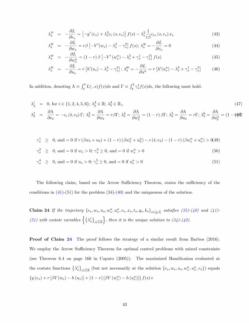
�10s = � @L@es

=��y0 (es) + �3sce (s; es)

�f(s)� �2s

1

r�cee (s; es)xs (43)

�20s = � @L@ws

= r���V 0(ws)� �3s � 2s

�f(s); �30s = �

@L

@vs= 0 (44)

�40s = � @L@wns

= (1� r)���V 0 (wns )� �3s + 1s � 3s

�f(s) (45)

�50s = � @L@us

= r�h0(us)� �3s � 4s

�; �60s = �

@L

@un= r

�h0(uns )� �3s + 1s � 5s

�(46)

In addition, denoting � �R ss L(�; s)f(s)ds and � �

R ss

1sf(s)ds, the following must hold.

�is = 0, for i 2 f1; 2; 4; 5; 6g; �3s 2 R; �3s 2 R+ (47)

�1s =@�

@es= �ce (s; es) �; �2s =

@�

@ws= r��; �4s =

@�

@wns= (1� r)��; �5s =

@�

@us= r�; �6s =

@�

@uns= (1� r) �(48)

1s � 0, and = 0 if r (�ws + us) + (1� r) (�wns + uns )� c (s; es)� (1� r) (�wns + uns ) > 0(49)

2s � 0, and = 0 if ws > 0; 3s � 0, and = 0 if wns > 0 (50)

4s � 0, and = 0 if us > 0; 5s � 0, and = 0 if uns > 0 (51)

The following claim, based on the Arrow Su¢ ciency Theorem, states the su¢ ciency of the

conditions in (41)-(51) for the problem (34)-(40) and the uniqueness of the solution.

Claim 24 If the trajectory fes; ws; us; wns ; uns ; vs; xs; ts; qs; ksgs2[s;s] satis�es (35)-(40) and (41)-

(51) with costate variablesn��isi21;6

o, then it is the unique solution to (34)-(40).

Proof of Claim 24 The proof follows the strategy of a similar result from Barbos (2016).

We employ the Arrow Su¢ ciency Theorem for optimal control problems with mixed constraints

(see Theorem 6.4 on page 166 in Caputo (2005)). The maximized Hamiltonian evaluated at

the costate functions��isi21;6 (but not necessarily at the solution fes; ws; us; w

ns ; u

ns ; vsg) equals

fy (es) + r [�V (ws)� h (us)] + (1� r) [�V (wns )� h (uns )]g f(s)+

43

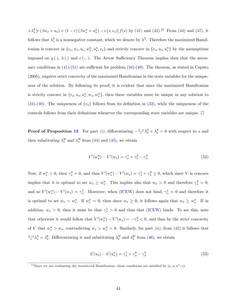
+�3s [r (�ws + us) + (1� r) (�wns + uns )� c (s; es)] f(s) by (41) and (42).23 From (44) and (47), it

follows that �3s is a nonnegative constant, which we denote by �3. Therefore the maximized Hamil-

tonian is concave in fes; ws; us; wns ; uns ; vsg and strictly concave in fes; us; uns g by the assumptions

imposed on y (�), h (�) and c (�; �). The Arrow Su¢ ciency Theorem implies then that the neces-

sary conditions in (41)-(51) are su¢ cient for problem (34)-(40). The theorem, as stated in Caputo

(2005), requires strict concavity of the maximized Hamiltonian in the state variables for the unique-

ness of the solution. By following its proof, it is evident that since the maximized Hamiltonian

is strictly concave in fes; us; uns ; ws; wns g, then these variables must be unique in any solution to

(34)-(40). The uniqueness of fvsg follows from its de�nition in (33), while the uniqueness of the

controls follows from their de�nitions whenever the corresponding state variables are unique. �

Proof of Proposition 13 For part (i), di¤erentiating �1�rr �2s + �

4s = 0 with respect to s and

then substituting �20s and �40s from (44) and (45), we obtain

V 0(wns )� V 0(ws) = 1s + 2s � 3s (52)

Now, if wns > 0, then 3s = 0, and thus V

0(wns ) � V 0(ws) = 1s + 2s � 0, which since V is concave

implies that it is optimal to set ws � wns . This implies also that ws > 0 and therefore 2s = 0,

and so V 0(wns ) � V 0(ws) = 1s. Moreover, when (ICEW) does not bind, 1s = 0 and therefore it

is optimal to set ws = wns . If wns = 0, then since ws � 0, it follows again that ws � wns . If in

addition, ws > 0, then it must be that 1s > 0 and thus that (ICEW) binds. To see this, note

that otherwise it would follow that V 0(wns ) � V 0(ws) = � 3s < 0, and thus by the strict concavity

of V that wns > ws, contradicting ws > wns = 0. Similarly, for part (ii), from (42) it follows that

1�rr �

5s = �

6s. Di¤erentiating it and substituting �

50s and �

60s from (46), we obtain

h0(us)� h0(uns ) = 1s + 4s � 5s (53)

23Since we are evaluating the maximized Hamiltonian, these conditions are satis�ed by (e; u; un; v).

44

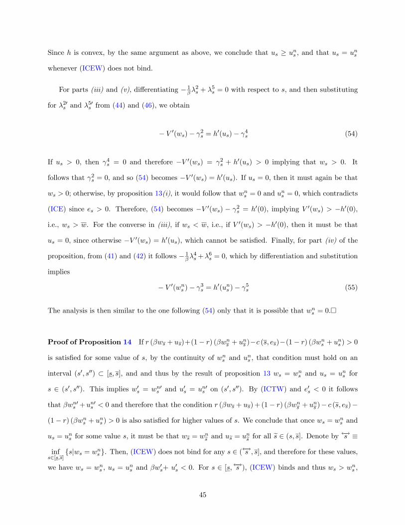
Since h is convex, by the same argument as above, we conclude that us � uns , and that us = uns

whenever (ICEW) does not bind.

For parts (iii) and (v), di¤erentiating � 1��2s + �

5s = 0 with respect to s, and then substituting

for �20s and �50s from (44) and (46), we obtain

� V 0(ws)� 2s = h0(us)� 4s (54)

If us > 0, then 4s = 0 and therefore �V 0(ws) = 2s + h0(us) > 0 implying that ws > 0. It

follows that 2s = 0, and so (54) becomes �V 0(ws) = h0(us). If us = 0, then it must again be that

ws > 0; otherwise, by proposition 13(i), it would follow that wns = 0 and uns = 0, which contradicts

(ICE) since es > 0. Therefore, (54) becomes �V 0(ws) � 2s = h0(0), implying V 0(ws) > �h0(0),

i.e., ws > w. For the converse in (iii), if ws < w, i.e., if V 0(ws) > �h0(0), then it must be that

us = 0, since otherwise �V 0(ws) = h0(us), which cannot be satis�ed. Finally, for part (iv) of the

proposition, from (41) and (42) it follows � 1��4s +�

6s = 0, which by di¤erentiation and substitution

implies

� V 0(wns )� 3s = h0(uns )� 5s (55)

The analysis is then similar to the one following (54) only that it is possible that wns = 0.�

Proof of Proposition 14 If r (�ws + us)+(1� r) (�wns + uns )�c (s; es)�(1� r) (�wns + uns ) > 0

is satis�ed for some value of s, by the continuity of wns and uns , that condition must hold on an

interval (s0; s00) � [s; s], and and thus by the result of proposition 13 ws = wns and us = uns for

s 2 (s0; s00). This implies w0s = wn0s and u0s = un0s on (s0; s00). By (ICTW) and e0s < 0 it follows

that �wn0s +un0s < 0 and therefore that the condition r (�ws + us)+ (1� r) (�wns + uns )� c (s; es)�

(1� r) (�wns + uns ) > 0 is also satis�ed for higher values of s. We conclude that once ws = wns and

us = uns for some value s, it must be that wes = wnes and ues = unes for all es 2 (s; s]. Denote by !s �

infs2[s;s]

fsjws = wns g. Then, (ICEW) does not bind for any s 2 ( !s ; s], and therefore for these values,

we have ws = wns , us = uns and �w

0s+ u0s < 0. For s 2 [s; !s ), (ICEW) binds and thus ws > wns ,

45

us � uns (with us > uns if us > 0) and �wns +uns = 11�r [r (�ws + us) + (1� r) (�w

ns + u

ns )� c (s; es)],

the latter implying �wn0s + un0s = 0. (ICTW) implies then that �w

0s+ u

0s < 0.

We will argue next that it must be that w0s < 0 and u0s � 0. As shown above, for all s, we have

�w0s+ u0s < 0. When ws � w, and thus us = 0, this immediately implies that w0s < 0 and u0s = 0.

When ws > w, since us > 0, we have from the proof of proposition 13 that V 0(ws) + h0(us) = 0.

This implies that w0s and u0s have the same sign. To see this, note that if, for instance, w

0s > 0

and u0s < 0, then as es increases in a neighbourhood of s, both V 0(wes) and h0(ues) strictly decrease,implying that V 0(wes)+h0(ues) = 0 cannot hold. �w0s+ u0s < 0 implies then that w0s < 0 and u0s < 0.Similarly, since as argued above, for all s 2 [s; !s ), we have �wn0s +un0s = 0, whereas from the same

proof of proposition 13 we have that V 0(wns ) + h0(uns ) = 0 when wns > w, it follows by a similar

argument that wn0s = 0 and un0s = 0. �

Proof of Proposition 15 Di¤erentiating �1s + �2s1r� ce (s; es) = 0 with respect to s, and then

substituting for �10s and �20s from (43) and (44), we obtain

� y0 (es) f(s)� V 0(ws)ce (s; es) f(s) + �2s1

r�ces (s; es) = 0 (56)

Integrating �20s from (44) between s and s while accounting for �2s = 0 and for the fact that

2s = 0 for all s since ws > 0, we obtain �2s = �r�

R ss

�V 0(w�) + �

3�f(�)d�. Applying the Dynamic

Envelope Theorem to problem (34)-(40), we have that V 0(w) = ��3. Substituting �3 into the

expression obtained for �2s we obtain

�2s = r�

Z s

s

�V 0(w)� V 0(w�)

�f(�)d� (57)

Substituting �2s into (56), we conclude that (8) from the text of the proposition must hold. �

Proof of Remark 16 From (57), we have �20s = r� [V0(w)� V 0(ws)] f(s). Note that d

ds [V0(ws)] =

V 00(ws)w0s > 0 since V is strictly concave and w0s < 0 by proposition 14. Therefore V

0(ws) is strictly

46

increasing in s and thus there exists some s0 2 [s; s] such that �V 0(w) + V 0(ws) < 0 if and only if

s > s0. Since f(s) > 0, this implies �20s < 0 if and only if s > s0. Therefore, �2s is increasing for small

values of s and then decreasing. Since from (47)-(48), we have �2s = 0 and �2s = r�

R ss

1sf(s)ds � 0,

these imply that indeed �2s > 0 for all s 2 (s; s), and therefore the remark follows from (57). �

Proof of Proposition 18 The argument relies on the proof of the corresponding result for the

static model in Barbos (2016). Thus, let es = e0s and ws = wns = u

ns = 0 for all s 2 [s; s], and let

us � us � 1r

R ss ce(�; e

0�)e

00� d�. By the same steps as in Barbos (2016), it follows that if w = 0, then

rus = c�s; e0s

��Z s

scs�s; e0s

�F (s)ds (58)

us needs to be non-negative because of the limited liability of the agent, which is precisely the

assumption from the text of the proposition 18. As argued in Barbos (2016), us � 0 is su¢ cient for

all incentive constraints to be satis�ed.24 By the same argument as in the proof of proposition 10,

since A�s initial continuation value is 0, one can implement the �rst best e¤ort in every period with

the above contract by maintaining a continuation value equal to 0 at the beginning of every period.

Since A�s expected wage equals that under full information, it folllows then that the contract de�ned

above is optimal since its value attains the theoretical upper bound. �

Proof of Proposition 17 Using the multipliers from the de�nition of L, the per-period change

in P�s payo¤ from a small increase in r is

�V =

Z s

s

@

@rL (�; s) f(s)ds

=

Z s

sf[�V (ws)� h (us)]� [�V (wns )� h (uns )]g f(s)ds+

Z s

s�2s

�1

r2

�ts +

1

�ks

�� 1

�r2ce(s; es)xs

�ds

+

Z s

s

��3s [(�ws + us)� (�wns + uns )] + 1s [(�ws + us)� (�wns + uns ) + (�wns + uns )]

f(s)ds

24We employ here the underlying assumption that e0s > 0 for all s 2 [s; s].

47

Using (36) and then (35), we have

1

r

�ts +

1

�ks

�� 1

r�ce(s; es)xsds = �w0s �

1

�u0s + w

n0s +

1

�un0s

Using this and (44), integrating by parts, we have then

Z s

s�2s

��ts +

1

�ks

�� 1�ce(s; es)xs

�ds =

=

��2s

��ws �

1

�us + w

ns +

1

�uns

������ss

�Z s

s�2s

��ws �

1

�us + w

ns +

1

�uns

�f(s)ds

= r�

��ws �

1

�us + w

ns +

1

�uns

�Z s

s 1sf(s)ds+r�

Z s

s

�V 0(ws) + �

3s

���ws �

1

�us + w

ns +

1

�uns

�f(s)ds

Substituting these results into the expression for �V derived above, and cancelling out terms, we

have that

�V =

Z s

sf[�V (ws)� h (us)]� [�V (wns )� h (uns )]g f(s)ds+

+

Z s

sV 0(ws) (��ws � us + �wns + uns ) f(s)ds+

Z s

s 1s (�w

ns + u

ns ) f(s)ds

=

Z s

s

��V (ws)� h (us)� �V (wns )� h (uns )� �V 0(ws)ws

�f(s)ds+

�Z s

sV 0(ws)usf(s)ds+ �

Z s

s

�V 0(ws) +

1s

�wns f(s)ds+

Z s

s

�V 0(ws) +

1s

�uns f(s)ds

Now, note �rst that from (54) and 2s = 0, we have �V 0(ws) = h0(us)� 4s, so �V 0(ws)us = h0(us)us

since 4sus = 0 by the complementary slack condition. Second, from (52) we have V 0(ws) + 1s =

V 0(wns ) + 3s, so

�V 0(ws) + 1s

��wns = �V 0(wns )w

ns since

3sw

ns = 0. Finally, from (54) and then

(53) we have V 0(ws) = 4s � h0(us) = 4s �� 1s +

4s � 5s + h0(uns )

�) V 0(ws) + 1s =

5s � h0(uns ).

Therefore,�V 0(ws) + 1s

�uns = �h0(uns )uns since 5suns = 0. Collecting all these results, it follows

48

that

�V = �

Z s

s

��V (ws)� V 0(ws)ws

���V (wns )� V 0 (wns )wns

�f(s)ds+

+

Z s

s

��h0(us)us � h(us)

���h0 (uns )u

ns � h (uns )

�f(s)ds (59)

Note now that the function V (w) � V 0(w)w is increasing in w since V is concave. Since from

proposition 13, we have ws � wns , the �rst integral in (59) is thus positive. Similarly, the function

h0(u)u� h(u) is increasing in u since h is convex. Since us � uns , the second integral in (59) is also

positive. By the same argument as in the proof of proposition 9, since the per-period change to

P�s payo¤ from a small increase in r is positive, it follows that V (w), which is the discounted sum

of future period payo¤s, is increasing in r. This completes the proof of proposition 17. �

References

[1] Barbos, A. (2016): "Optimal Contracts with Random Monitoring".

[2] Biasi, B., T. Mariotti, J-C. Rochet and S. Villeneuve (2013): "Large Risks, Limited Liability,

and Dynamic Moral Hazard," Econometrica, 78, 73-118.

[3] Caputo, M. R., (2005): Foundations of Dynamic Economic Analysis, Cambridge University

Press, Cambridge, UK.

[4] Fraser, R. (2012): "Moral Hazard, Targeting and Contract Duration in Agri-Environmental

Policy," Journal of Agricultural Economics, 63, 56-64.

[5] Kovrijnykh, N. (2013): "Debt Contracts with Partial Commitment," American Economic

Review, 103, 2848-2874.

[6] Ok, E.A. (2007): Real Analysis with Economic Applications, Princeton University Press,

Princeton, NJ.

49

[7] Radner, R. (1981): "Monitoring Cooperative Agreements in a Repeated Principal-Agent Re-

lationship," Econometrica, 49, 1127-1148.

[8] Rockafellar, R.T. (1970): Convex Analysis, Princeton University Press, Princeton, New Jersey.

[9] Rogerson, W. (1985): "Repeated Moral Hazard," Econometrica, 53, 69-76.

[10] Sannikov, Y. (2008): �A Continuous-Time Version of the Principal-Agent Problem,�Review

of Economic Studies, 75, 957-984.

[11] Spear, S.E. and S. Srivastava (1987): "On Repeated Moral Hazard with Discounting," Review

of Economic Studies, 54, 599-617.

[12] Spear, S. and C. Wang (2005): "When to Fire a CEO: Optimal Termination in Dynamic

Contracts," Journal of Economic Theory, 120, 239-256.

[13] Stokey, N.L. and R.E. Lucas (1989): Recursive Methods in Economic Dynamics, Harvard

University Press, Cambridge, MA.

[14] Sundaram, R.K. (1996): A First Course in Optimization Theory, Cambridge University Press,

Cambridge, UK.

[15] Townsend, R. (1982): "Optimal multiperiod contracts, and the gain from enduring relation-

ships under private information," Journal of Political Economy, 90, 1166-1186.

50